Factors Affecting Commercial BankLending to Agriculture

Eustacius N. Betubiza and David J. Leatham*

Abstract

A tobit econometric procedure was used to examine the effect of selected demand andsupply factors on nonreal estate agricultural lending by commercial banks in Texas. Results showthat banks have reduced their agricultural loan portfolios in response to increased use of interestsensitive deposits after deregulation, Moreover, almost half of this decrease came from banks thatstopped making agricultural loans. Also, results show that banks affiliated with multi-bank holding

companies lend less money to agriculture relative to their assets than do independent banks.

Key Words: agricultural lending, commercial banks, deregulation, tobit

Commercial banks have traditionally playedan important role in financing agriculture. Their

commitment to agriculture, however, fluctuates. Forexample, between 1968 and 1987 their market sharein nonreal estate farm lending in the U.S. rangedfrom a high of 66.8 percent (9.7 billion dollars) in1968, to a low of47.3 percent (32.8 billion dollars)in 1981, closing at 53, I percent in 1987 (Walraven

and Rosine). The fluctuation in the market share is

a combination of the adjustment in the volume offunds lent by banks to the agriculture sector and the

adjustment in the number of banks lending to theagriculture sector. In Texas, the proportion ofbanks with zero agricultural loans outstandingincreased from 16,6 percent in 1968 to 35.5 percentin 1987. Between 1980 and 1987, 9 I commercial

banks, which had been active agricultural lenders inthis period, had zero nonreal estate agriculturalloans outstanding in 1987. Many factors have led

to these fluctuations in agricultural lending.

It is expected that recent deregulation ofcommercial banks has affected agricultural lending.Since the passage of the Depository Institutions

Deregulation and Monetary Control Act of 1980

(particularly with the elimination of interest rateceilings -- commonly known as regulation Q) bankshave increased their competitiveness in acquiringloanable funds, mainly in form of time deposits(Bundt and Schweitzer; Waldrop; Keely andZimmerman). However, these time deposits areassociated with higher and more variable costs that

increase the overall risk of the bank operation.Moreover, changes in the type and characteristics ofa bank’s loanable finds can elicit a realignment ofthe bank’s asset portfolio to reflect the newcomposition of its liabilities.

The competition for Ioanable funds has aneffect on the cost and availability of loan finds toagricultural borrowers. Borrowing costs go up aslenders attempt to transfer some of these higher

costs incurred in acquiring funds to borrowers.Loan funds to agricultural borrowers may be

curtailed, for example, as banks seek to match theirinterest rate sensitive liabilities with interest rate

sensitive, nonloan assets. Banks might increasesecurity requirements, or decrease the term of theloan. Banks might also opt to increase the

supervision of the loans to increase performance.

*Eustacius N. Betubiza is an economist at the World Bank, Washington, D.C., and David J. Leatham is an associate

professor of Agricultural Economics at Texas A&M University, College Station, Texas. Technical Article No. 30813of the Texas Agricultural Experiment Station.

J Agr, and Apphed Econ. 27 (l), July, 1995: 112-126Copyright 1993 Southern Agricultural Economics Association

J Agr. and Apphed Econ,, July, 1995 113

However, because increased supervision is costly to

the bank, loans may only be extended to those

borrowers with a more than “usual” likelihood ofrepayment, thus excluding many potential farmborrowers.

A tobit econometric procedure was used inthis study to examine the effects of selected demandand supply factors on agricultural lending. Inparticular, the impact that increased commercialbank reliance on the interest sensitive deposits after

deregulation has on funds that banks allocate toagriculture relative to other investment opportunities

was examined. Also, independent banks werecompared to multi-bank holding company (MBHC)affiliates to determine the impact of bankorganization on the share of agricultural loans intheir asset portfolios.

There were 1053 Texas banks included inthis study. Each of these banks was in businessbefore deregulation ( 1978) and after deregulation(1987). In 1978, 7.3 percent and 25.8 percent ofthe rural and urban banks were MBHC affiliates,respectively. By 1987, 24.3 percent and 56.9percent of the rural and urban banks were MBHCaffiliates, respectively, Thus, it is important tostudy the impact this move toward MBHCorganization has on agricultural lending. Althoughthe data used in this study are unique to Texas,inferences drawn can be extended to commercial

banks in the U.S,

Model Development

Tobil Procedure

As noted above, several banks haveeliminated agricultural loans from their portfolios,Therefore, an econometric analysis of an uncensuredsample of banks with agricultural loans as thedependent variable would have several zero values.In other words, the dependent variable is part

qualitative (to lend or not to lend) and partquantitative (the amount lent). The analysis of such

a limited dependent variable is called tobit analysis.This technique is designed to study models with a

dependent variable having the property that manyobservations take on a single value (as in zerodollars lent for agriculture), with the remainingobservations following the usual characteristic of acontinuous variable (dollars lent to agriculture), It

has received wide application to such problems as

the study of automobile purchases, models of labor

supply, and household purchase of fresh vegetables. 1

In his pioneering work, Tobin analyzedhousehold expenditure on durable goods as a

fimction of income and other variables. He notedthe distortion in the data resulting from the fact thatmany households did not purchase a durable goodduring the year of survey, with the possible

explanation that because expenditures on durable

goods are not continuous, purchases are not madeuntil the “desire” to buy the good exceeds a certain

level. However, desires cannot be observed, onlyexpenditures, and those will be nonzero only if the

good is purchased. “Negative” expenditures,

corresponding to various levels of desire below thethreshold level, cannot be observed, and allhouseholds with no purchases are recorded asshowing zero expenditure, with no distinction madebetween households who were close to buying thegood and those who had very little desire to do so.=

The same is true with commercial banks.There is a certain threshold beIow which a bankwould not effect an agricultural loan transaction (or

any loan transaction for that matter), although therewould be variations between different borrowers andlenders reflecting transaction costs, risks, etc.Lending is not done until the “desire” to lendexceeds a certain level. Desires, however, cannotbe observed. “Negative loans,” corresponding tovarious levels of desire below this threshold level

are recorded as zero agricultural loans, with nodistinction made between commercial banks that areclose to lending to agriculture and those that havevery little desire to do so. Previous research has

circumvented the problem of limited dependentvariables by excluding banks with zero agriculturalloans when investigating factors affecting

agricultural lending. Data samples have beenlimited to agricultural banks with existingagricultural loan portfolios (e.g., Barry and Pepper).This omission, however, creates sample selectionbias (Heckman, 1979). Rather than delete bankswith zero agricultural loans outstanding from the

sampie, tobit analysis is used to account for thisinformation and to adequately portray the full range

of commercial bank behavior (Tobin).

To understand this behavior, it is important

to note that the changes in commercial bank lending

114 BetubIzu and Lea(ham Factotx Af/ec(tng Cotnmerc/al Bank Lending to Agriculture

to the agricultural sector involve two types ofadjustments: a) changes in the number of bankslending to the agricultural sector, and b) changes in

the number and size of agricultural loans made bycommercial banks already lending to agriculture.The time-series observations on the changes in totalagricultural lending reflect both types of adjustment.However, it is impossible to estimate the separatetypes of adjustment from aggregate time-series data

based on average bank lending to the agriculturalsector (Thraen, et al.). Cross-sectional data, on theother hand, include observations on individual banks-. some of which are agricultural Iendcrs, and others

are not. One could estimate the quantity adjustmentcoefficients by exclusion of those banks that werenot lenders to agriculture at the time of the survey.However, it is also possible to estimate both the

lending volume adjustments of commercial banksalready lending to agriculture, and the lendingvolume adjustments due to the entry or exit ofbanks by using the tobit estimation procedure.

The Theoretical Model

Let

Y’xp+E (1)

be a regression equation for which all basic

assumptions are satisfied. For commercial banksthat made agricultural loans, Y is equal to the actual

agricultural loans made. For those banks that did

not, Y represents an index of the “desire” to makeagricultural loans. The X matrix is a set of factorsthought to affect Y. The ~ is a conformablydefined parameter vector, and E represents the

stochastic disturbance term of the regression.

The value of Y cannot be observed when

loans are not made. Thus, instead of using Y, ~ is

used and is defined as

Y(’=Yif Y>O

Y“=OifY30(2)

The new equation is

y<i = ‘yp + ~a (3)

where ~ is truncated at zero and & is truncated at- X ~, This further implies that the lower tail of the

distribution of Y’ (and thus of E“) is cut off and theprobabilities are piled up at the cut-off point.

Consequently, the mean of Y“is different from that

of Y, and the mean of EC’is different from that ofewhich is zero. This is true whether the points for

which Y’ equal zero arc included or not included inthe sample. Therefore, limiting the range of thevalues of the dependent variable leads to a nonzeromean of the disturbance and the biasness andinconsistency of the least squares estimators.

Equation (3) will be estimated using the

tobit procedure. The (3 parameters will be estimatedusing the maximum likelihood method (assuming

normality of the disturbance term). This procedureassures the large-sample properties of consistency

and asymptotic normality of the estimatedcoefficients so that conventional tests of significanceare applicable.

Following McDonald and Moffit, different

elasticities, evaluated at the means, can be computedas follows:

x-q.E[Y”] = - —, (4)

E[Y”]

x-rlEIY*] = _ —, and (5)

E[Y*]

13F(z) 7q F(z) = _ —.

ax F(Z)(6)

where q E[ Y“] is the elasticity of the unconditional

expected value of agricultural lending,,

qE[Y*] IS the elasticity of the conditional

expected value of agricultural lending,

q F(z) is the elasticity of the probability of

making agricultural loans,

F(z) denotes the cumulative standard normal

distribution function, and

E[Y”] is the conditional expected value of Y.

J Agr and Applied Econ, July, 1995 115

It can be shown that the sum of equations(5) and (6) is equal to equation (4) (McDonald andMoffit). In other words, the unconditional elasticityof making agricultural loans can be broken downinto its component parts: a) the elasticity of makingagricultural loans, for current lenders to agriculture,

and b) the elasticity of the probability of makingagricultural loans. By looking at the twocomponents, one can find out which componentreacts most to changes in the explanatory variables.Thus, besides the usual parameter estimates, thetobit procedure provides these elasticities that serveas a measure of the impact of changes in anindependent variable on agricultural lending, not justfor current agricultural lenders, but for those that

would quit or enter agricultural lending as well.

Variable Description

The Regressand

The model regressand, Y’, was defined asthe ratio of outstanding nonreal estate agriculturalloans to total bank assets for each commercial bank.Banks have different investment options, includingagricultural lending. Using total assets as thedenominator shows the relative importance ofagricultural loans in the bank’s investment program

by recognizing the nonloan investment optionsavailable to a bank (e.g., government securities) that

compete with agricultural loans for investable funds.This ratio increases/decreases ‘as more funds aremoved in/out of agriculture relative to otherinvestment opportunities. Farm real estate loanswere excluded from the study because commercialbanks, historically, have not offered significantamounts of this category of loans.

The Regressors

Thirteen model regressors (table 1) were

chosen to reflect the supply and demand factors

affecting Y’, These regressors included five bankvariables, six agricultural variables and two generalvariables. The five bank variables included in themodel, designed to capture factors affecting abank’s allocation of investable funds among

competing investment opportunities, are: the bank’sdeposit composition, the level of competition facedby the bank, its organizational structure (specifically

its association with a multi-bank holding company),

location, and equity base. The six agriculturalvariables included in the model are: farm

profitability, farm risk, value of farmland andbuildings, size of farming community, ownership offarmland, and the level of farm mechanization.These variables affect the degree to which

agriculture attracts investable funds from

commercial banks. The variables population and oilproduction were also included in the study becausethey are expected to affect the demand andavailability of commercial banks’ investable finds.Each variable is discussed below.

Deposit M-ucture

A ratio of a bank’s time and savings

deposits to total deposits (DEPOSIT) was used torepresent the proportion of total deposits that aresensitive to interest rate changes. It can be arguedthat there is a positive relationship betweenDEPOSIT and loans in general because time andsavings deposits enhance the stability of Ioanablefunds. Therefore, banks need less liquidity andcan invest more money in loans. h can also beargued that there is a negative relationship.Deposits are more interest rate sensitive and banksmay choose to increase investments in interest ratesensitive assets and to decrease investments in

loans, Banks may choose to invest in moreinvestment securities like U.S. treasury securities

because their interest rate movement more closelymatches the interest rate movements on deposits,thus, reducing interest rate risk. This may

especially be true in the post-deregulation era that ischaracterized by volatile interest rates. Banks coulduse adjustable interest rates on loans to make themmore sensitive to interest rate movements.

However, repricing a loan can result in additionaltransaction costs to the bank and transferring risk to

a borrower may increase the likelihood of a loan

default. It is not clear which effect overshadows the

other. Thus, the sign on the estimated coefficient is

indeterminate a priori.

Competition

The competition faced by an individual

bank in a certain community or sector (e.g.,agriculture) should affect its investment decisions.This is particularly true if there are specialized

lenders. The major competitor of commercial banks

116 Be!ubiza and Leatham: Factors Affecting Commercial Bank Lending to Agriculture

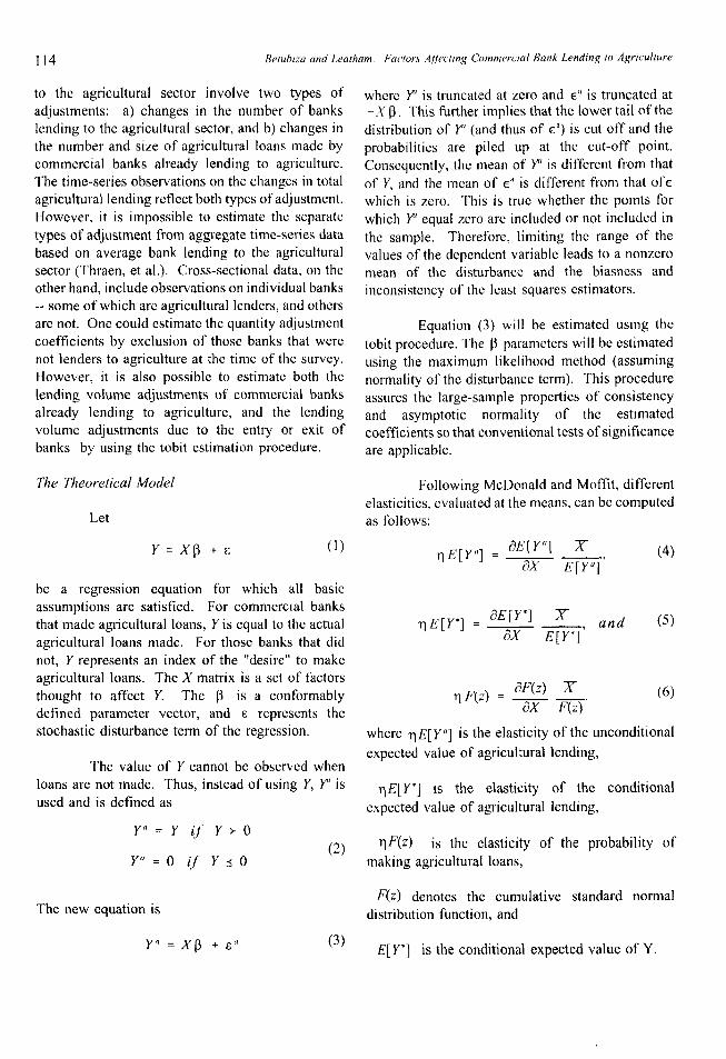
Table 1. Explanatory Variables m the Toblt Model

COMPETITION

MBHC

URBAN

EQUITY

PROFIT

RISK

LAND

INCOME

OWNER

MACHINE

POPULATION

OIL

.

—

.

.

ratio of a bank’s time and savings deposits to total deposits.

an index that measures the amount of competition a bank faces inits market area for agricultural loans.

binary variable: 1 If a bank belongs to a multl-bank holdingcompany.

binary variable: 1 If a bank is located in a metropohtan stahsticalarea

ratio of a bank’s total equity to M total assets.

ratio of net cash income from farm sales to total farm assets ineach county.

ratio of the coefficient of variation of farm income to the

coefficient of vanatlon of total income m each county.

value of land and bulldmgs ($1,000/acre, average) m each county.

ratio of farm Income to total income In each county

ratio of the number of farmers operating their own land to the totalnumber of farmers In each county.

eshmated market value of all machmery and equipment m thecounty ($ mlUmr).

Population m each county (1,000’s)

amount of 011produced m each county m 1987 (barrels).

in the nonreal estate farm loan market is ProductionCredit Associations (PCAS). A commercial bank islikely to allocate less money to agriculture relativeto its total assets in areas where PCAS and othercompeting commercial banks are very active. Thenumber of alternative credit sources in thecommunity has previously been used as a proxy forcompetition (Barkley et al,), However, this does not

consider the size of the competitors. In this study,

the proxy for bank competition was based on thevolume of assets of its competitors in its market. Abank’s market area was delineated by county

boundaries, Although this might not be true in allcases, it has been found a reasonable assumptionunder conditions where the study does not focus onlocal market characteristics and the flow of funds(Barry and Pepper; Gilbert). A competition indexwas computed that consisted of PCA assets andtotal assets of the commercial banks operating in the

same county, The proxy for competition faced by

a bank was computed as

compe~ition indexi = 1 - bank assets , (7)total assets

where the competition index (COMPETITION) is ameasure of the amount of competition faced by thejth bank in its market area, with O denoting laok ofcompetition and I denoting maximum competition;bank assets refer to the total assets of the jth bank;

and total assets refer to all the combined assets ofPCAS and commercial banks operating in the

county.

Multi-Bank Holding Company (MBHC) Affiliation

Barry and Pepper contend that bankholding company affiliation in general providesbanks with greater lending capacity, morecompetitive behavior, stronger risk bearing, moreflexible funds acquisition, and deeper service

capacity. Thus, MBHC affiliation should contributepositively to the availability of credit servicesoffered by smaller banks to agriculture. Following

this reasoning, a positive relationship would be

expected between MBHC affiliation and the

agricultural loan to asset ratio, reflecting the

affiliate’s greater capacity to generate loanable

J. Agr, and Applied Econ., July, 1995 117

finds, to meet large loan requests, to have more

specialized personnel, and to provide credit-relatedservices. However, MBHC affiliates might also

have more diverse clients and investmentopportunities that might compete for their Ioanablefunds resulting in reduced agricultural lendingrelative to total assets. A dummy variable was

defined, with a 1 for multi-bank holding companyaffiliation and O otherwise. It is not possible, a

priori, to determine the sign of the estimatedcoefficient.

Urban

Urban banks (URBAN), defined as thosebanks located in a standard metropolitan statisticalarea, have more diverse clients and thus have moreflexibility in moving in and out of agriculture.Moreover, rural banks are more likely to lend moremoney to agriculture relative to their assets thanurban banks because rural banks are moredependent on the agricultural economy. Thus, anegative estimated coefficient would be expected forurban banks.

Farm Profitability

A firm that is achieving a high rate of

return on its assets can increase the return to equityby increasing its leverage, as long as the rate ofreturn on assets exceeds the rate of interest paid onfarm debt (Collins). Thus, farmers in a county withprofitable farming operations would demand moreagricultural loans. Similarly, banks in such a

county would be willing to commit a higherproportion of their asset portfolio to agriculturalloans because of the reduced likelihood of loan

defaults by the farm borrowers. This variable,which was defined as the ratio of net cash incomefrom farm sales to total farm assets in each county(PROFIT), is expected to have a positivecoefficient.

Farm Risk

The ratio of the coefficient of variation offarm income to the coefficient of variation of totalincome in each county (RISK) was used as a

measure of farm risk. It is expected that countieswith higher farm risk would attract less agriculturallending from commercial banks. Thus, the

estimated coefficient should be negative.Equity

Value of Farmland and BuildingsAn important function of bank capital is to

reduce risk, Koch discusses three ways in whichthis is achieved. First, it provides a cushion forfirms to absorb losses and remain solvent. Second,it provides ready access to financial markets andthus guards against liquidity problems caused bydeposit outflows. Third, it constrains growth andlimits risk taking. A well-capitalized institution isin a better position to take on risk by investing

more in loans and less in safe assets likegovernment securities. Its large equity base would

cushion the institution against large loan losses.However, the decision makers of less capitalizedinstitutions may choose a similar investmentstrategy to increase expected profits, although at agreater risk. It is consistent with this risk/returnpreference for them to invest in more risky assetssuch as loans because of their higher expectedreturns. Thus, the estimated coefficient of the equity

variable, which was defined as the ratio of the

bank’s total equity to its total assets (EQUITY), isindeterminate.

A lender can reduce the likelihood of loanlosses by requiring that land be used as collateral onnonreal estate loans. A farm located in an area withhigh farmland and property values will likely havea higher collateral value. Higher collateral valuessupport higher levels of debt. The property valuewas standardized across communities by dividing

the total value of farmland and farm buildings in a

county by the total acres of farmland (LAND).

An area with high farm property values,

however, may also be in an area that offers greaternonagricultural business opportunities. In fact,

such areas will likely be located near commercialand industrial centers. These commercial andindustrial businesses (and consumers in the

communities) will compete for bank loans. Thus,

agricultural loan portfolios of commercial banks inthese areas may be smaller. Therefore, the sign ofthe estimated coefficient is indeterminate, a priori.

118 Be/ul)/za and Lea[ham Factors A//iec//ng Commercial B&k Lending 10 Agrudture

Size qf Farming Community

Banks located in predominantly agriculturalcommunities will likely obtain a large percentage of

their deposits from farm firms. To cultivate astrong bank-borrower relationship, these banks arelikely to lend a greater proportion of their investable

funds to the local farming community. Moreover,

there is a feedback effect, by which a thriving localcommunity will increase the deposits, providingmore Ioanable funds for the bank. However,specializing in agriculture can lead to financialdifficulties for the bank in case of an economicdownturn in the local economy. The ratio of farmincome to total income in each county (INCOME),which was used as a proxy for the size of thefarming community, is expected to have a positiveestimated coefficient.

Ownership of Farmland

It is likely that owner-operators would beinterested in developing and maintaining a more

long term relationship with their Icndcrs than tenantfarmers. Thus, in general, lending to an owner-operator would be less risky than lending to a tenantfarmer because owner-operators would likely havea longer farming history and loan collateral on land.In fact, several credit scoring studies have foundland ownership to be an important factor indiscriminating between potentially good agriculturalloans and bad loans (Dunn and Frey; Luiburrow,

Barry and Dixon; Reinsel). However, there are

other important credit factors such as managementability, repayment ability, and borrower integrity,factors that are not unique to owner operators.Moreover, tenant farmers may not have as muchequity capital as owner-operators and may requiremore nonreal estate financing. The ownership offarmland variable, defined as the ratio of thenumber of farmers operating their own land to thetotal number of farmers in each county (OWNER),is expected to have a positive estimated coefficient.

Level of Farm Mechanization

Counties with more mechanized operationsare assumed to require more debt capital to financeequipment and operating expenses. Thus, thisvariable, defined as the estimated market valueof all machinery and equipment in the county

(MACHINE), is expected to have a positiveestimated coefficient.

Population

Population was used as a proxy forconsumer loan demand in each county. Nonfarmpopulation is expected to provide deposits to

commercial banks, thus, providing banks withadditional loanable funds. However, the nonfarm

population will also compete with farmers for theseloanable funds. Thus, the expected sign of theestimated coefficient is indeterminate a priori.

Oil Production

An economy strengthened by increased oilrevenue benefits agriculture as a whole, much as aneconomy weakened by a loss of oil revenue hurts

agriculture. Besides providing loanable fi.rnds, oilrevenues also affect the purchasing power of those

who depend on agriculture for food and fiber.However, this model was not designed to capturethese interrelationships. It is easy to predict theeffect of an oil boom or burst on the generaleconomy of a given state, but it is more difficult toassess its impact on a local farming community.Oil production will stimulate the local economy

directly from employment and oil producingbusiness activities, and indirectly from oil profitsretained in the community. The increase in

economic activity may lead to an increase in local

deposits, thus increasing banks’ loanable funds.However, the increase in economic activity willIikcly increase loan demand for working capital,expansion of nonagricultural businesses, andconsumer loans that compete with agricultural loans.The estimated coefficient is, therefore, indeterminate

a priori.

Data Sources

Data on bank variables were obtained from

the FDIC call reports on condition and income, and

agriculture data came from the Census of

Agriculture (USDA, 1978 and 1987). Population

and per capita income figures came from the Local

Area Personal Income’ publications of the U.S.Department of Commerce, and oil production

figures came from the Railroad Commission of

Texas. Loan information for each PCA was

J, Agr. and Applied Econ,, July, 1995 119

obtained directly from personnel at the Farm Credit

Bank of Texas. It was estimated that loans were 80percent of total PCA assets. Total PCA assetswere apportioned among counties by assigningweights to assets based on the value of farm outputper county relative to the total value of farm outputin the PCA area.

Results

Summary Statistics

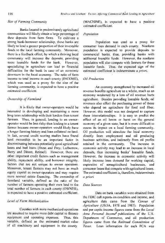
Rural banks invested an average of I Ipercent of their assets in nonreal estate agriculturalloans (agricultural loan portfolio) in 1978 (table 2).However, this percentage dropped to 7.6 percent forrural independent banks and 6.6 percent for MBHCaffiliates in 1987. Urban banks have experiencedsimilar, but less dramatic, decreases as well. Part ofthis drop may be traced to deregulation, particularly

to the high levels of interest rate sensitive deposits

that have characterized the post deregulation era,However, there have also been some importantchanges in the agricultural and banking sector overthis period.

Rural independent banks held fewer timeand savings deposits to total deposits (55 percent )in 1978, than rural MBHC affiliates (58 percent)(table 2). These ratios rose to 83 percent and 84

percent respectively, in 1987. Urban banks held 57percent of their deposits in time and savings

deposits in 1978, and 82 percent in 1987. Thisimportant increase in interest sensitive depositslikely increased the banks’ cost of funds and itsvolatility, which in turn influenced the asset

allocation decisions made by each bank.

Average bank equity ratios in 1978 ranged

from a low of 7.3 percent (Urban MBHC affiliates)to a high of 8.9 percent (Rural Independent) (table

2). After deregulation, equity ratios decreased by1.9, 1.2, and 0.4 percentage points for urban and

rural MBHC affiliates, and urban independents,respectively. Capital increased by 0.4 percentagepoints for rural independent banks.

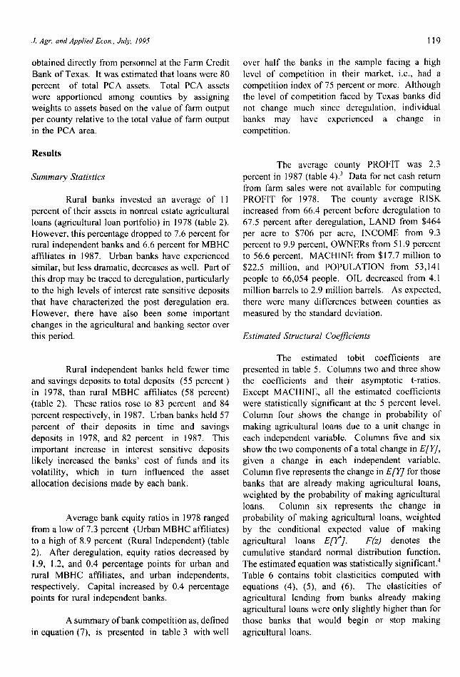
A summary of bank competition as, defined

in equation (7), is presented in table 3 with well

over half the banks in the sample facing a highlevel of competition in their market, i.e., had a

competition index of 75 percent or more. Althoughthe level of competition faced by Texas banks didnot change much since deregulation, individualbanks may have experienced a change incompetition.

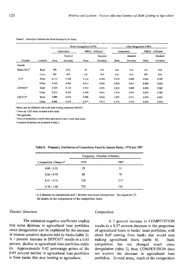
The average county PROFIT was 2.3

percent in 1987 (table 4).3 Data for net cash returnfrom farm sales were not available for computingPROFIT for 1978. The county average RISK

increased from 66.4 percent before deregulation to67.5 percent after deregulation, LAND from $464

per acre to $706 per acre, INCOME from 9.3percent to 9.9 percent, OWNERS from 51.9 percentto 56.6 percent, MACHINE from $17.7 million to

$22.5 million, and POPULATION from 53,141people to 66,054 people. OIL decreased from 4.1

million barrels to 2.9 million barrels. As expected,there were many differences between counties asmeasured by the standard deviation.

Estimated Structural Coefficients

The estimated tobit coefficients arepresented in table 5. Columns two and three showthe coefficients and their asymptotic t-ratios.Except MACHINE, all the estimated coefficientswere statistically significant at the 5 percent level.

Column four shows the change in probability ofmaking agricultural loans due to a unit change in

each independent variable. Columns five and sixshow the two components of a total change in E/_Y],

given a change in each independent variable.Column five represents the change in E[Y] for thosebanks that are already making agricultural loans,weighted by the probability of making agricultural

loans. Column six represents the change inprobability of making agricultural loans, weighted

by the conditional expected value of makingagricultural loans E@]. F(z) denotes the

cumulative standard normal distribution function.The estimated equation was statistically significant.4Table 6 contains tobit elasticities computed withequations (4), (5), and (6). The elasticities ofagricultural Iending from banks already makingagricultural loans were only slightly higher than forthose banks that would begin or stop making

agricultural loans.

120 Muhizo and Lea[ham: Factors Affecting Commercial Bank Lending 10 Agrmd(ure

Table 2 Descriptive Stausticsfor Banks hIcludcd in tlw Study

Before Dcmgulatioo ( 1978) Aflcr Oercgulalion ( 1987)

[dependent MBIIC. Aftillates’ Independent MBNC - A~llates’

Standard Standard Standard Stmdard

Var!able Location Mean Devmtton Mean Deviation Mean Deviation Mean Deviation

Sample

Banks (No )’ Rund 496 N/AC 39 N/A 414 NIA 133 NIA

~Jtb,III 384 NIA I 34 NIA 218 NIA 288 NIA

[Y’]’ Rural 0,112 0 I(J8 0112 0.102 0076 0,089 0,066 0.089

Urban 0036 0,060 0.01I 0,030 0,020 0031 0.009 0,022

DEPOSIT Rural 0549 0132 0.582 0091 0832 0,099 0,84tl 0083

Urbau 0573 0101 0,569 0,065 0816 0,06 I 0,820 0.062

EQUI 1Y“ Rural 0.089 0.024 0088 0,022 0.093 0041 0,076 0025Urban 0,080 0019 0073 0015 0,076 0030 0,054 0,030

‘ Banks O1atarc aftllirhl with multi-bank holding companIes (MBIIC)

b I here arc 1,053 bnoks iricludcd in this study,

‘ No! applicable.

‘ Ratio of outstanding nonreal estateagricultural loans to total bank assets

‘ Complete definitions are presented in table 1,

Table 3. Frequency Distribution of Competition Faced by Sample Banks, 1978 and 1987

Frequency (Number of Banks)

Competition Category’ 1978 1987

0.00-0.25 29 31

0.26-0.50 68 70

0.51-0.75 226 217

0.76-1.00 730 735

`A Odenotes nocompet]tion andldenotes maximum competition, See equation(7)

for details on the computation of the competition index,

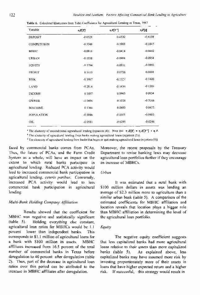
Deposit Structure

The estimated negative coefficient impliesthat some decrease in agricultural loan portfolios

since deregulation can be explained by the increasein interest sensitive deposits held by banks (table 2).A I percent increase in DEPOSIT results in a 0.85

percent decline in agricultural loan portfolios (table6). Approximately 0,42 percentage points of the0.85 percent decline in agricultural loan portfoliosis from banks that stop lending to agriculture.

Competition

A 1 percent increase in COMPETITIONresults in a 0.37 percent decrease in the proportion

of agricultural loans in banks’ asset portfolios, withabout half coming from banks that would stopmaking agricultural loans (table 6). Bankcompetition has not changed much since

deregulation (table 3), thus, COMPETITION doesnot explain the decrease in agricultural loan

portfolios. In rural areas, much of the competition

J, Agr. and Applied Econ , July, /995

Table 4. County Summary Statistics for the Non Bank Variables Used m the Toblt Model, 1978 and 1987,(Number of Counties= 254~

1978 1987

Standard Standard

Variable Mean Deviation Mean Deviation

PROFIT b b. . . . . . 0.023 0.030

RfSK 0,664 0.284 0675 0194

LAND 0.464 0262 0706 0.478

INCOME 0093 0.105 0.099 0133

OWNER 0519 0.137 0.566 0.126

MACHINE 17.678 15.237 22.452 15.665

POPULATION 53.141 191.280 66.054 239.050

OIL 4.099 10.513 2.854 6.641

‘ Varrable name detlnitions arepresented in table 1. Dollar values arem nominal terms.h Nol Available

Table5. Summ~Sbtistics for Tobit Analysis oftie Mmmdmd Supply of A~culmmlh ndingtiTexm,1987

AsympoticVariable P I-ratio

[%1 I-94 [%~’”rDEPOSIT o.0648~ -2.61 -0.3646 -0,0229 -0,0222

COMPETITION -0,0286d -243 -0.1641 -0.0103 -0,0)00

MBHC -0.0112” -2.64 -0.0401 -0.0025 -00024

URBAN -o.oz!9d -4.26 -0.1426 -0.009 -0.0087

EQUITY -0. 1496d -2.56 -0.8261 -0.05 I9 -0,0503

PROFIT 0.S163~ 4.81 2,9687 0.1865 0.1808

Rf.w -0.0287’ -2.21 -0,1670 -0.0105 -0.0102

LAND -0.0198’ -2.85 -0.0898 -0,0056 -0.0055

INCOME 0.2391’ 7.77 1.3974 0.0878 0.0851

OWNER -0.1038d -4.14 -0.6138 -0.0386 -00374

MACHINE o,~765 I .74 1.6536 0.1039 01007

POPULATION -0.0146d -3,67 -0.0850 -00053 -0.0052

OIL -o.oo13d -3.86 -0.0076 -0.0005 -0.0005

CONSTANT o.~ 163d 7.08 ] ,2577 0.0790 0.0766

‘ Chmgektie probabillV ofmaking agriculwral loans duetoachange inthecowesponding independent

variable.

b Change LnEfY'forthose bamksalready making agricultural loans, weighted bytheprobability of making

agricultural loans.

C Change intheprobabili~ ofmaking agricultural ioans, weighted bytheconditional expected value of

making agricultural loans E[Y ].

d Significant atthe5 percent level.

Note: The standard error around the Tobit index is 0.0580. The predicted probability that Y> O,at the measr

of X, is 0.7191, and Theil’s goodness-of-fit stmstic is 0.3762.

122 Be!uhiza and Leatham: Fac[or.s Affecting Commercial Bank Lending [o Agriculture

Table 6. Calculated 131astlcttlesfrom Tobit Cue fticients for Agnadtund Lending m Texas, 1987

DEPOSIT

COMPETITION

M13HC

URBAN

EQUITY

PROFIT

RISK

LAND

INCOME

OWNER

MACHINE

POPULATION

OIL

-0,8528

-03748

-0.0816

-01938

-01794

01410

-03007

-02816

01897

-10494

01364

-00986

-00581

-0.4330

-0.1903

-0.0414

-00984

-0.0911

00716

-0.1527

-01430

0.0963

-0,5328

0,0693

-0,0501

-00295

-0.4198

-0.1845

-0.0402

-0.0954

-00883

0.0694

-01480

-01386

00934

-05166

0.0672

-0,0485

-00286

aTheelmtlclty ofuncondlllonal agricultural lendlng (cquatlon (4)). Note that ~E[~ - qE[l’”] + qfi.

b The clastlclty of agricultural lendlng from banks malang agricultural loans (equation (5)).

‘ The clastlclty of agncukural lemhng from banks that begin or qwt maktng agricultural loans (equation (6)).

faced by commercial banks comes from PCAS.Thus, the future of PCAS, and the Farm CreditSystem as a whole, will have an impact on theextent to which rural banks participate inagricultural lending. Reduced PCA activity wouldlead to increased commercial bank participation in

agricultural lending, ceteris paribus. Conversely,increased PCA activity would lead to less

commercial bank participation in agriculturallending.

Multi-Bank Holding Company Afjlia~ion

Results showed that the coefficient forMBHC was negative and statistically significant

(table 5). Holding everything else constant,agricultural loan ratios for MBHCS would be 1. Ipercent lower than independent banks. Thiscorresponds to $1.1 million of agricultural loans for

a bank with $100 million in assets. MBHCaffiliates increased from 16.5 percent of the totalnumber of commercial banks in Texas before

deregulation to 40 percent afler deregulation (table2). Thus, part of the decrease in agricultural loanratios over this period can be attributed to theincrease in MBHC affiliates afier deregulation.

Moreover, the recent proposals by the TreasuryDepartment to revise banking laws may decreaseagricultural loan portfolios further if they encouragean increase of MBHCS.

Urban

Itwas estimated that a rural bank with

$100 million dollars in assets was lending anaverage of $2.3 million more to agriculture than asimilar urban bank (table 5). A comparison of theestimated coefficients for MBHC affiliation andlocation reveals that location plays a bigger rolethan MBHC affiliation in determining the level ofthe agricultural loan portfolio.

Equity

The negative equity coefficient suggeststhat less capitalized banks had more agriculturalloans relative to their assets than more capitalized

banks (table 5). As explained above, lesscapitalized banks may have assumed more risk byinvesting proportionately more of their assets inloans that have higher expected return and a higherrisk, If successful, this strategy would result in

J. Agr. and Applied Econ., July, 199S

greater profits relative to the capital committed.

However, the negative relationship could be a

reflection of the poor performance of the

agricultural sector in the early 1980’s. Banksmaking agricultural loans could have incurred heavyloan losses eroding the loan loss reserves of theseinstitutions.

Farm Profitability

As expected, results show that

communities with more profitable farmingoperations attract more agricultural loans than

communities with less profitable farming operations(table 5). Thus, part of the observed decline inagricultural loan portfolios at Texas commercialbanks since deregulation was a reflection of thedeclining performance of the agricultural sector inTexas in the 1980’s relative to the 1970s. A I

percent decrease in PROFIT results in a 0.14

percent decrease m agricultural loan portfolios

(table 6).

Farm Rikk

In counties where farm income is relativelymore volatile than nonfarm income, less money islent to agriculture compared to other investment

opportunities (table 5). A 1 percent increase inRISK results in a 0.30 percent decrease in

agricultural loan portfolios (table 6), Thus, part of

the observed decline in the agricultural loanportfolios at commercial banks since deregulationwas a result of the increased risk in production

agriculture (table 4).

Value of Farm Land and Buildings

Results show that a 1 percent increase in

LAND decreases agricultural loan portfolios by 0,28

percent (table 6). A possible explanation for thisunexpected result is the high valued property’sproximity to urban centers, where nonagricultural

activities are likely to compete more favorably forbank investments.

Size of Farming Community

The positive estimated coefficient of theproxy for the importance of agriculture in a countyis expected because a bank located in apredominantly farming community depends on

123

agriculture for borrowers and on farm related

income for its deposits (table 5). However,INCOME did not increase much atler deregulation,offering little explanation for the decline in bank

agricultural loan portfolios (table 4).

Ownership of Farm Land

The negative estimated coefficient suggests

that owner-operators borrow less nonreal estate debtfrom banks than tenant farmers (table 5), contrary tothe previously stated hypothesis that land ownership

corresponds to high agricultural loan ratios. A

possible explanation is that tenant farmers on theaverage have less equity capital, thus requiringgreater financing of operating expenses and

machinery. It is also possible that the owner-

operators that obtain their land loans from theFederal Land Bank may also obtain nonreal estateloans from PCAS. This result may also be dataspecific. Nonreal estate debt is reported as a real

estate debt in the FDIC call reports when land isused as collateral. Thus, nonreal estate debt may beunder-reported for owner-operators.

Level of Farm Mechanization

The estimated coefficient of farm

machinery was not statistically significant, although

it had the expected positive sign (table 5),suggesting little correlation between the level of

agricultural loan portfolios at commercial banks, andthe value of farm machinery in the respectivecommunities.

Population

The more populated counties attracted

money away from agriculture, with a 1 percentincrease in POPULATION resulting in a 0.10

percent decrease in agricultural loan portfolios (table6).

Oil Production

The results suggest that agriculture was nota major beneficiary from “petro-dollars” in oilproducing counties. A 1 percent decrease in OIL

results in a 0.06 percent decrease in agriculturalloan portfolios (table 6).

124 Be(uhiza and Leatham: Factor.r Affecting Commercial Bank Lending (o Agriculture

Summary and Conclusions

A tobit econometric procedure was used toexamine the effect of selected demand and supplyfactors on the proportion of agricultural loans incommercial bank asset portfolios. In particular, theimpact of increased commercial bank reliance oninterest sensitive deposits after deregulation on

funds that banks allocate to agriculture relative toother investment opportunities was examined. Also,independent banks were compared to multi-bankholding company affiliates to determine the impact

of bank organization on the share of agriculturalloans in bank asset portfolios.

Results show that as commercial bankdeposits become more sensitive to market rates,

the proportion of agricultural loans relative to

commercial bank assets decline. A 1 percent

increase in the ratio of time and savings deposits tototal deposits was associated with 0.85 percentdecline in the ratio of agricultural loans to total

assets, with almost half of this decline coming frombanks that would stop making agricultural loans.Also, banks affiliated with multi-bank holdingcompanies lend less money to agriculture relative to

their assets than do nonmulti-bank holding companyaffiliates. Thus, as multi-bank holding companyaffiliates continue to increase (e.g., throughacquisitions of failed institutions by existing bankingorganizations or through voluntary mergers), therewill be a reduction in agricultural loans providedrelative to the volume of assets held by commercialbanks, which could mean an absolute reduction in

the total amount of loans available to the

agricultural sector.

References

Amemiya, T. “Regression Analysis When the Dependent Variable is Truncated Normal,” Econometrics4I(1973):997-1016.

Barkley, David L., Cindy Mellon, and Glenn T. Potts. “Effects of Banking Structure on the Allocation ofCredit to Nonmetropolitan Communities.” W. J, ,4gr. Econ. 9( 1984):283-92.

Barry, Peter J., and W.H. Pepper. “Effects of Holding Company Afllliation on Loan-Deposit Relationships

in Agricultural Banking.” NC J, Agr. Econ, 7( I985):65-73.

Bundt, Thomas P., and Robert Scheitzer. “Deregulation, Deposit Markets, and Banks’ Costs of Funds.”The Fin. Rev. 24(1 989):41 7-30.

Capps, Oral Jr., and John M. Love, “Determinants of Household Expenditure on Fresh Vegetables.” S. J.Agr. Econ, 15(December, 1983): 127-32,

Gilbert, R. Alton. “Requiem for Regulation Q: What It Did and Why It Passed Away.” Federal Reserve

of St. Louis. Review 68( February 1986):22-37.

Gragg, J. G. “Some Statistical Models for Limited Dependent Variables with Application to the Demand

for Durable Goods.” Econometrics 39( 197 I):829-44.

Hagemann, Robert P. “The Determinants of Household Vacation Travel: Some Empirical Evidence.”

Applied Econ. 13(1981): 225-34

Heckman, J. J. “Shadow Price, Market Wages and Labor Supply.” Econometrics 42( 1974):679-94.

Heckman, J. J. “The Common Structure of Statistical Models of Truncation, Sample Selection and Limited

Dependent Variables and a Simple Estimator for Such Models,” Annals of Econ. and Sot.

Measure. 5(1976):475-92.

J. Agr and Applied Econ , July, 1995 125

Heckman, J. J. “Sample Selection Bias as a Specification Error,” Econometrics 47( 1979): 153-61.

Keeley, Michael C., and Gary C. Zimmerman. “Competition of Money Market Deposit Accounts.”Proceedings: A Conference on Bank Structure and Competition, pp. 612-35, Federal Reserve Bank

of Chicago (May, 1985)

Kmenta, Jan. Elem. of Econometrics, New York: MacMillan Publishing Company, Inc., 1986.

Koch, Timothy W. Bank Management, Orlando, Florida: The Dryden Press, 1988,

McDonald, J. F., and R.A. Moffitt. “The Uses of Tobit Analysis. ” Rev. of Econ. and Statist.62(1980):318-21.

Railroad Commission of Texas. Oil and Gas Annual Report. Oil and Gas Division, Austin, Texas, severalissues.

Thraen, C. S., I.W. Hammond, and B,M. Buxton. “Estimating Components of Demand Elasticities from

Cross-Sectional Data.” Am. J Agr. Econ. 60(1978):674-77.

Tobin, James. “Estimation of Relationships for Limited Dependent Variables.” Econometrics26(1958):24-36,

U.S. Department of Agriculture. Census qfAgr. Government Printing Office, Washington D.C., severalissues.

U.S. Department of Commerce. Local Area Personal Income 1983-88. Volume 5: Southwest, Rocky

Mountain, and Far West Regions and Alaska and Hawaii. Bureau of Economic Analysis.Government Printing Office,Washington D,C. July, 1990.

Waldrop, R. “Interest Rate Deregulation and Its Impact on the Cost of Funds at Commercial Banks.”Banking and Econ. Rev. 4( March 1986): 19-22.

Walraven, N. A., and John Rosine. Agr. Fin. Data. Board of Governors of the Federal Reserve System.Washington D.C. April, 1989.

Endnotes

1, For some theoretical discussion see J. Tobin, T, Amemiya, and J. Heckman. For some applications,see J. Heckman, and J.G. Gragg. For a more recent application in the agricultural economics literature,see O. Capps Jr. and John M. Love.

2. Another common example of a limited dependent variable relates to the wages of married women sincewages are recorded only for women who are in the labor force. Wages of women whose “reservation wage”exceeds their market wage and who, therefore, stay at home are recorded as zero. No distinction is made

between women whose reservation wage barely exceeds their market wage and those whose reservationwage is much higher than their market wage. (J. Kmenta, p. 561).

126 Betubiza and Leatham: Facvors Affecting Commercial Bank Lending to Agriculture

3. The Agricultural Census Bureau derives the cash return from agricultural sales for the farm unit bysubtracting operating expenditures from the gross market value of agricultural products sold. Depreciationand the change in inventory values are excluded from expenditures. Gross sales include sales by theoperator andtheshare ofsales received bypafiners, landlords, and contractors, This ratio does not includecapital gains. Farm assets were defined as the sum of the market value of land and buildings, and themarket value of machinery and equipment.

4. A test using the chi-square distribution replaces the usual F test to test the significance of all the

coefficients in the tobit model when maximum likelihood is used. First, the likelihood function is evaluatedwhen all parameters other than the constant are set to zero (LO). Next, the likelihood function at itsmaximum (L~,X) is evaluated. The likelihood ratio test is constructed as -2(1 og LO- log L~,X) -Xz,p wherep is the number of regressors in the statistical model,