Embed Size (px)
Citation preview

The Practicalities of Libor Market Models
Peter Jäckel
There are many publications on the theory of the Libor market model andits extensions. There are very few sources on the issues a pracitionerfaces during implementation and opertion of the model. This presentationis on the subject of how to make a Libor Market Model work in practice.
The Practicalities of Libor Market Models 1
Contents
I. Standard and skewed Libor market model dynamics 3
II. Derivation of the indirectly stochastic drift 16
III. Leaving the canon 22
IV. Futures convexity corrections in the Libor market model 27
V. Speed is everything — the predictor-corrector scheme 39
VI. Parametrisation of correlation and volatility backbone 44
VII. Factor reduction — pros and cons 49
Contents Peter Jäckel
The Practicalities of Libor Market Models 2
VIII. Speed is everything — the drift term 53
IX. Analytical calibration to coterminal swaptions 58
X. Non-parametric volatility specification 75
XI. Global calibration to the full swaption matrix 80
XII. Bermudan Monte Carlo 97
XIII. Cross-currency Libor market modelling 144
XIV. Calibration of FX volatilities in a cross-currency Libor market model 151
Contents Peter Jäckel
The Practicalities of Libor Market Models 3
I. Standard and skewed Libor market model dynamics
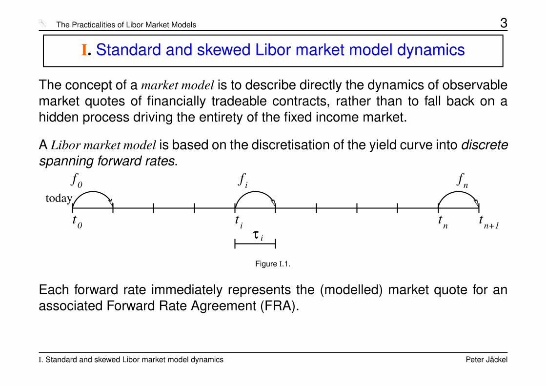
The concept of a market model is to describe directly the dynamics of observablemarket quotes of financially tradeable contracts, rather than to fall back on ahidden process driving the entirety of the fixed income market.
A Libor market model is based on the discretisation of the yield curve into discretespanning forward rates.
tnt0
f0
t i
f i
iτtn+1
fn
today
Figure I.1.
Each forward rate immediately represents the (modelled) market quote for anassociated Forward Rate Agreement (FRA).
I. Standard and skewed Libor market model dynamics Peter Jäckel
The Practicalities of Libor Market Models 4
A forward rate agreement quote fi for period ti → ti+1 with accrual factor τi 'ti − ti+1 means:
• Upon deposit of a notional at time ti, at the later time ti+1 the notional plusinterest amounting to fi · τi times the notional is returned to the depositor.
• For a borrower of money, the effetive funding discount factor over the (for-ward) interval ti → ti+1 is given by 1/ (1 + fiτi).
The fair value of a Forward Rate Agreement on rate fi struck at K is
P (t, ti+1) · (fi −K) τi
where P (t, ti+1) is the value at time t of a zero coupon bond paying one domesticcurrency unit at time ti+1.
At time ti, the value becomes (fi −K) τi/ (1 + fiτi).
I. Standard and skewed Libor market model dynamics Peter Jäckel

The Practicalities of Libor Market Models 5
In the standard Libor market model for discretely compounded interest rates,we assume that each of n spanning forward rates fi evolves according to thestochastic differential equation
dfifi
= µLNi (f , t)dt+ σi(t)dWi . (1)
This ensures that all interest rates remain positive at all times.
Note:the drift terms are yet to be determined by the aid of no-arbitrage arguments!
Correlation is incorporated by the fact that the n standard Wiener processes inequation (1) satisfy
E[dWi dWj
]= ρijdt . (2)
The elements of the instantaneous covariance matrix C(t) of the n forward ratesare thus
cij(t) = σi(t)σj(t)ρij . (3)
I. Standard and skewed Libor market model dynamics Peter Jäckel

The Practicalities of Libor Market Models 6
Using a decomposition of C(t) into a pseudo-square root A such that
C = AA> , (4)
we can transform equation (1) to
dfifi
= µLNi dt+
∑j
aij dWj (5)
with dWj being n independent standard Wiener processes where dependenceon time has been omitted for clarity.
The matrix A is sometimes also referred to as the driver, or as the dispersion1
matrix, or even as the factor loading matrix.
Note : it is not advisable to assume that ti+1 − ti ≡ τ for some constant τfor all i since the error incurred by this approximation is too large.
1Karatzas and Shreve [KS91], page 284.
I. Standard and skewed Libor market model dynamics Peter Jäckel
The Practicalities of Libor Market Models 7
A commonly used extension is to introduce an implied volatility skew by permit-ting the Libor rates to experience a displaced diffusion [Rub83]:
d(fi + si)fi + si
= µDDi (f , s, t) dt+ σDD
i dWi . (6)
This model can be calibrated comparatively easily to at-the-forward impliedvolatility σ := σ(f) quotes and the skew at the forward,
σ = ζ + 1−β2
24 ζ3T + 7−10β2+3β4
1920 ζ5T 2 +O(ζ7)
(7)
ζ = σ + β2−124 σ3 T + 3−10β2+7β4
1920 σ5 T 2 +O(σ7)
(8)
dσ(K)dK
∣∣∣K=f
= −(1−β)2
σf ·[1 + 1
12σ2T + 1
240σ4T 2 + 1
6720σ6T 3 +O
(σ8)], (9)
where we have used the parametrisation
σDDi = βiζi and si = (1− βi)
fi(0)βi
. (10)
I. Standard and skewed Libor market model dynamics Peter Jäckel
The Practicalities of Libor Market Models 8
Another common extension is to introduce Constant Elasticity of Vari-ance [Bec80, CR76, Sch89, AA00]:
dfi = µCEVi (f ,β, t) dt+ σCEV
i fβCEVi
i dWi . (11)
For moderate maturities, the following expansions can be used for calibration:
σ = σCEV · f(βCEV−1)(0) +O(σCEV3
)(12)
σCEV = σ · f(1−βCEV)(0) +O(σ3)
(13)
dσ(K)dK
∣∣∣K=f
= −(1−β)2
σf +O
(σ3), (14)
I. Standard and skewed Libor market model dynamics Peter Jäckel

The Practicalities of Libor Market Models 9
For longer maturities, one ought to use the general CEV option pricing formula
E[(f −K)+] ={
f ·Q(a, 2 + b, c)−K · [1−Q(c, b, a)] for β < 1f ·Q(c,−b, a)−K · [1−Q(a, 2− b, c)] for β > 1 (15)
with
a =K2(1−β)
(1− β)2 σCEV2 T(16)
b =1
1− β(17)
c =f(0)2(1−β)
(1− β)2 σCEV2 T(18)
and Q(a, b, c) being the complementary non-central χ2 distribution function for bdegrees of freedom and non-centrality parameter c.
I. Standard and skewed Libor market model dynamics Peter Jäckel
The Practicalities of Libor Market Models 10
Note: the Constant Elasticity of Variance distribution has a continuous and adiscrete part due to the fact that for β < 1 and t > 0 there is a positive probabilitythat f = 0. To avoid confusion with your implementation, we have defined allterms by the complementary distribution function.
The implied volatility surfaces of the displaced diffusion model and the constantelasticity of variance model are very similar for a wide range of strikes and skewcoefficients β. However, the constant elasticity of variance model does not per-mit long time step Monte Carlo integration methods as efficiently as the dis-placed diffusion model.
This is why the displaced diffusion model is very frequently used to match amarket observable implied volatility skew.
I. Standard and skewed Libor market model dynamics Peter Jäckel

The Practicalities of Libor Market Models 11
��������
��������
�������
������
��������
��������
���
���
����
���
���
��
����
����
���
���
���
���
��
��
���
Figure I.2. Implied volatilities for CEV model withf = 5%, β = 1/4, ζ = 30%.
��������
��������
�������
������
��������
��������
���
���
����
���
���
��
����
����
���
���
���
���
��
��
���
Figure I.3. Implied volatilities for displaced diffusion model withf = 5%, β = 1/4, ζ = 30%.
I. Standard and skewed Libor market model dynamics Peter Jäckel

The Practicalities of Libor Market Models 12
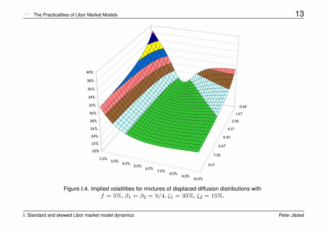
Neither the displaced diffusion nor the constant elasticity of variance model givescontrol over the smile, i.e. the curvature of the implied volatility profile.
An old option market maker trick to account for uncertainty in the implied volatilityaway from the money was to take the average of two Black prices for slightlydifferent implied volatilities.
Mathematically, this is consistent with the decomposition of the risk neutral den-sity into the weighted sum of two individually given lognormal probability densityfunctions.
Implying the single associated Black volatility that reproduces those optionprices results in an implied volatility smile. It can be shown, however, that thisapproach cannot reproduce a pronounced skew.
Applying the price mixing trick to the displaced diffusion model gives control overboth smile and skew.
I. Standard and skewed Libor market model dynamics Peter Jäckel
The Practicalities of Libor Market Models 13
2.0%3.0%
4.0%5.0%
6.0%7.0%
8.0%9.0%
10.0%
0.42
1.67
2.92
4.17
5.42
6.67
7.92
9.17
20%
22%
24%
26%
28%
30%
32%
34%
36%
38%
40%
Figure I.4. Implied volatilities for mixtures of displaced diffusion distributions withf = 5%, β1 = β2 = 3/4, ζ1 = 35%, ζ2 = 15%.
I. Standard and skewed Libor market model dynamics Peter Jäckel
The Practicalities of Libor Market Models 14
CAVEAT: Not all authors and practitioners agree on the meaningfulness of thisapproach when used literally by mixing the prices from calculations with differentmodel parameters [Pit03c].
However, since the distribution mixing is independent from the underlying spotprocess, it is possible to reproduce the precise smile from the mixture of twodisplaced diffusion distributions, both with the same displacement but differentdiffusion parameters, in the framework of a local volatility model.
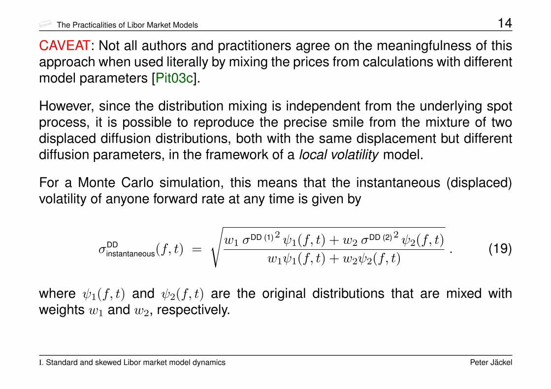
For a Monte Carlo simulation, this means that the instantaneous (displaced)volatility of anyone forward rate at any time is given by
σDDinstantaneous(f, t) =
√w1 σDD (1)2ψ1(f, t) + w2 σDD (2)2ψ2(f, t)
w1ψ1(f, t) + w2ψ2(f, t). (19)
where ψ1(f, t) and ψ2(f, t) are the original distributions that are mixed withweights w1 and w2, respectively.
I. Standard and skewed Libor market model dynamics Peter Jäckel
The Practicalities of Libor Market Models 15
Alas, this approach, like the genuine CEV model, makes it impossible to acco-modate long time steps efficiently.
Another way to model forward Libor rates in order to capture the skew and smileis to make the instantaneous volatility of a displaced diffusion model indepen-dently stochastic [Pit03a].
In this presentation, we restrict ourselves to the modelling of the level and theskew of implied volatilities by virtue of the displaced diffusion model.
We will, though, take into account a
term structure
of both
volatility and correlation.
I. Standard and skewed Libor market model dynamics Peter Jäckel
The Practicalities of Libor Market Models 16
II. Derivation of the indirectly stochastic drift
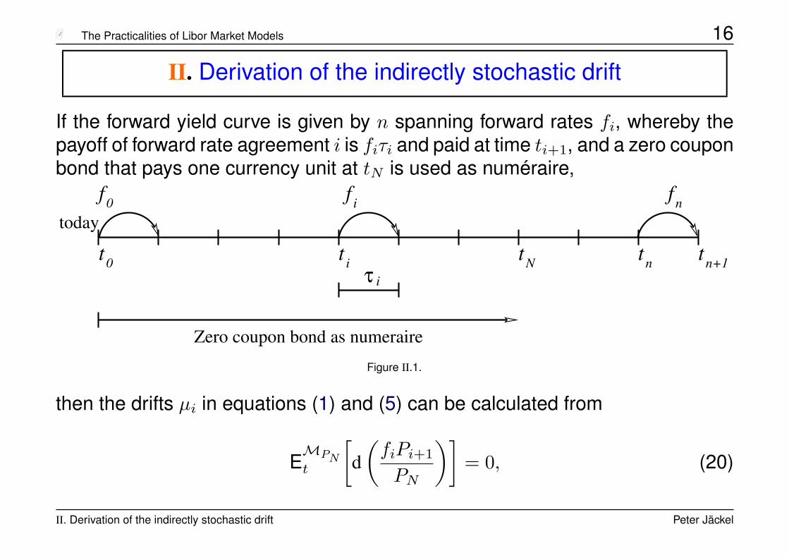
If the forward yield curve is given by n spanning forward rates fi, whereby thepayoff of forward rate agreement i is fiτi and paid at time ti+1, and a zero couponbond that pays one currency unit at tN is used as numéraire,
tN tnt0
f0
t i
f i
iτtn+1
f
Zero coupon bond as numeraire
n
today
Figure II.1.
then the drifts µi in equations (1) and (5) can be calculated from
EMPNt
[d(fiPi+1
PN
)]= 0, (20)
II. Derivation of the indirectly stochastic drift Peter Jäckel
The Practicalities of Libor Market Models 17
where Pi, ∀ i = 0, . . . , n are the ti discount bonds and
EMPNt [·]
the expectation operator under the equivalent martingale measure induced bythe choice of the discount bond PN as numéraire.
By the fundamental theorem of asset pricing, for the market to be free of arbi-trage, all ratios of tradeable assets divided by the numéraire value have to formmartingales [HP81], i.e. we also require
EMPNt
[d(PiPN
)]= 0, ∀ i = 0, . . . , n, (21)
since the discount bonds are assumed to be traded assets. Now, introducingthe bond ratio
Xi := Pi+1/PN (22)
and invoking Itô’s formula on equation (20) yields
EMPNt [Xidfi + fidXi + dfidXi] = 0 . (23)
II. Derivation of the indirectly stochastic drift Peter Jäckel
The Practicalities of Libor Market Models 18
Since dX is drift-free (it is an asset divided by the numéraire), this reduces to
EMPNt [Xi dfi + dXi dfi] = E
MPNt [Xiµifidt] + E
MPNt [dXi dfi] = 0 . (24)
In the following, we use the instantaneous relative covariance brackets [a, b]defined by the instantaneous drift of the product of the infinitesimal relative in-crements of any two stochastic processes a and b, i.e.
[a, b] := E[
daa
dbb
]/dt . (25)
The definition (25) immediately gives us
[a, bc] = [a, b] + [a, c] (26)
and[a, b/c] = [a, b]− [a, c] . (27)
II. Derivation of the indirectly stochastic drift Peter Jäckel
The Practicalities of Libor Market Models 19
Using this notation, we return to the derivation of the drift of the discrete forwardrates. From equation (24), we obtain
µi = −[fi,Pi+1
PN
](28)
which can be evaluated to:[fi,Pi+1
PN
]= [fi, Pi+1]− [fi, PN ]
=[fi,Πi
k=0(1 + fkτk)−1]−[fi,ΠN−1
k=0 (1 + fkτk)−1]
= −i∑
k=0
[fi, 1 + fkτk] +N−1∑k=0
[fi, 1 + fkτk] . (29)
II. Derivation of the indirectly stochastic drift Peter Jäckel
The Practicalities of Libor Market Models 20
By the definition of the bracket (25) and the dynamics of the individual forwardrates (1), each of the terms in the sums on the right hand side of equation (29)can be computed:
[fi, 1 + fkτk] =fkτk
1 + fkτkσiσkρik (30)
Finally, cancellation of summation terms leads to the drift formulæ
µ(tN)i (f(t), t) =
−σi
N−1∑k=i+1
fk(t)τk1+fk(t)τk
σkρik for i < N − 1
0 for i = N − 1
σii∑
k=N
fk(t)τk1+fk(t)τk
σkρik for i ≥ N
(31)
Note that this means that the drift of all of the forward rates but one are indirectlystochastic, i.e. it is stochastic due to its explicit dependence on the stochasticforward rates themselves. When i = N −1, i.e. for a drift-free forward rate fi, wecall the numéraire associated with the pricing measure the natural numéraire ofthe forward rate fi.
II. Derivation of the indirectly stochastic drift Peter Jäckel
The Practicalities of Libor Market Models 21
Computing the drift terms in different measures is readily accomplished by eval-uation of the effect of the change from
measureMA induced by numéraire NA
to
measureMB induced by numéraire NB
on the driving Wiener processes:
dWMB = E[
d ln(
dMB
dMA
)· dWMA
]+ dWMA (32)
with the Radon-Nikodym derivative
dMB
dMA=
NBNA· NA(0)NB(0)
. (33)
II. Derivation of the indirectly stochastic drift Peter Jäckel
The Practicalities of Libor Market Models 22
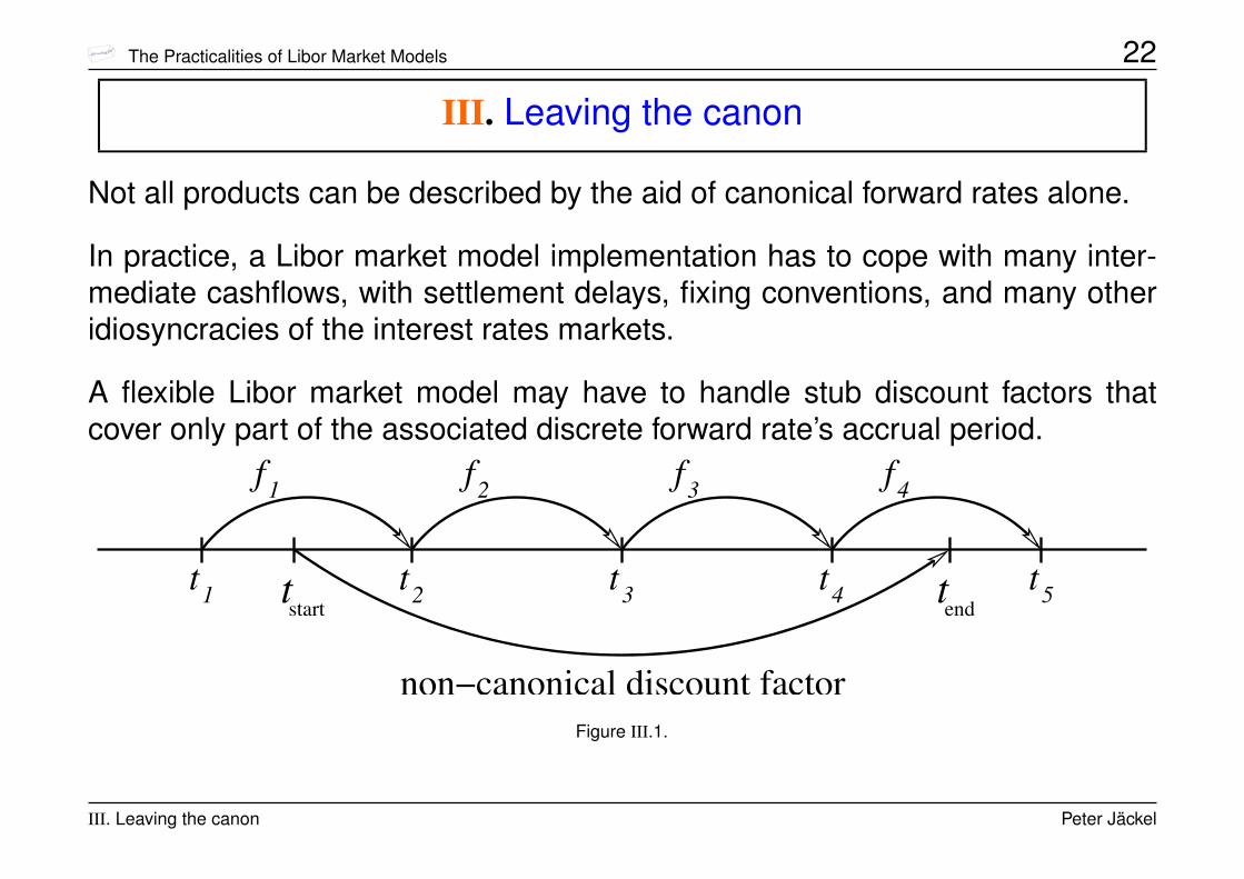
III. Leaving the canon
Not all products can be described by the aid of canonical forward rates alone.
In practice, a Libor market model implementation has to cope with many inter-mediate cashflows, with settlement delays, fixing conventions, and many otheridiosyncracies of the interest rates markets.
A flexible Libor market model may have to handle stub discount factors thatcover only part of the associated discrete forward rate’s accrual period.
f f 3f f
t1 t2 t3 t4 t5
1 2 4
t tstart end
non−canonical discount factorFigure III.1.
III. Leaving the canon Peter Jäckel

The Practicalities of Libor Market Models 23
It is difficult to construct non-canonical discount factors from a given set of dis-crete forward rates in a completely arbitrage-free manner.
However, in practice, it is usually sufficient to choose an approximate interpo-lation rule such that the residual error is well below the levels where arbitragecould be enforced.
It is also important to remember that the numerical evaluation of any complexdeal with a Libor market model is ultimately still subject to inevitable errors re-sulting from the calculation scheme: Monte Carlo simulations, non-recombiningtrees, or recombining trees with their own drift approximation problems.
In this context it may not be surprising that the following discount factor interpo-lation approach is highly accurate for practical purposes.
III. Leaving the canon Peter Jäckel
The Practicalities of Libor Market Models 24
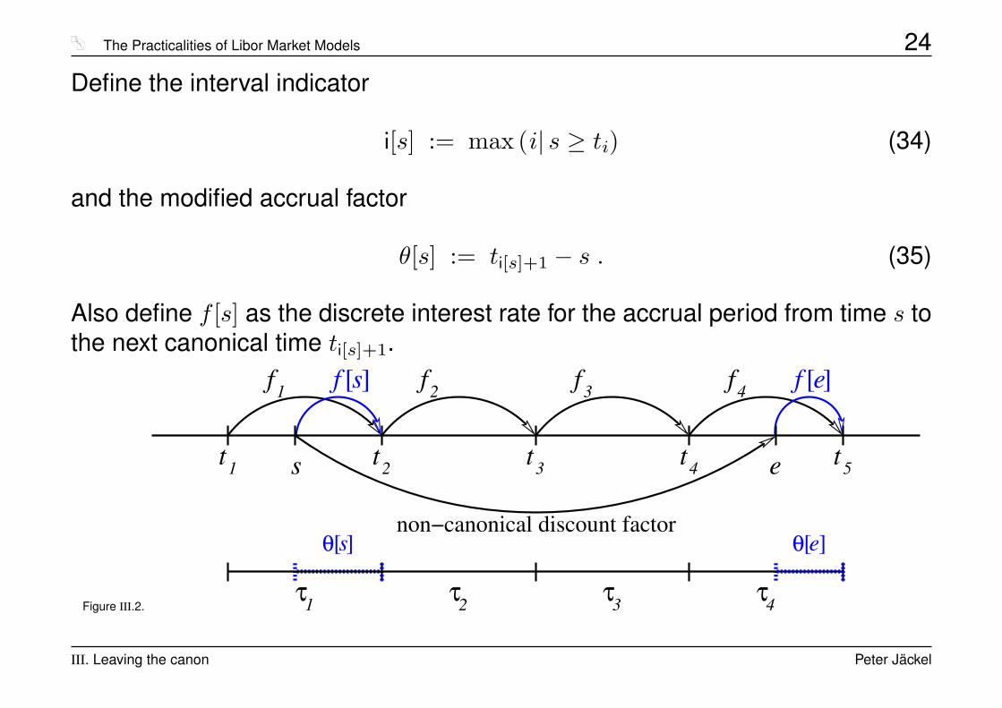
Define the interval indicator
i[s] := max (i| s ≥ ti) (34)
and the modified accrual factor
θ[s] := ti[s]+1 − s . (35)
Also define f [s] as the discrete interest rate for the accrual period from time s tothe next canonical time ti[s]+1.
Figure III.2. 2τ1τ τ4
f [ ]s f [ ]ef f 3f f
t1 t2 t3 t4 t5
1 2 4
τ3
s e
θ s][non−canonical discount factor
θ e][
III. Leaving the canon Peter Jäckel

The Practicalities of Libor Market Models 25
A forward discount factor thus decomposes into
P [s, e](t) =P (t, e)P (t, s)
=1 + f [e](t) · θ[e]1 + f [s](t) · θ[s]
i[e]+1∏j=i[s]+1
11 + fj(t)τj
. (36)
An approximation that for practical purposes suffices is to set
f [s](t) = γ[s] · fi[s](t) (37)
wherein the constant γ[s] takes care of the fine structure of the yield curve inbetween canonical dates as seen at inception:
γ[s] =f [s](0)fi[s](0)
=
(P (0,s)
P (0,ti[s]+1) − 1)/
θ[s]
fi[s](0). (38)
This approach essentially approximates the yield curve dynamics in betweencanonical times by a one factor model.
III. Leaving the canon Peter Jäckel

The Practicalities of Libor Market Models 26
Note: Since we decompose all stub rates into pieces depend-ing directly only on a canonical rate of the same natural mea-sure, it is straightforward to extend this model to allow for
stochastic stub rates
in between ti[s] and s by simply continuing the nominal statevariable fi[s] as a stochastic process all the way until ti[s]+1
instead of freezing it at ti[s] .
The generic interpolation rule (37) then takes care of the eval-uation of f [s] both for
t < ti[s]
and forti[s] ≤ t ≤ ti[s]+1 .
III. Leaving the canon Peter Jäckel

The Practicalities of Libor Market Models 27
IV. Futures convexity corrections in the Libor market model
The value of a future contract on a forward rate fixing at time ti is given by the ex-pectation of fi in the spot measure (also known as the measure associated withthe chosen numéraire being the continuously rolled up money market account)2:
fj = E∗[fj(tj)] (39)
In the discretely rolled up spot measure, we have
d(fj + sj)fj + sj
= µ∗jDD (f , s, t) dt+ σDD
j dW ∗j (40)
with
µ∗jDD (f , s, t) = σDD
j (t) ·j∑
k=i[t]+1
(fk(t) + sk)τk1 + fk(t)τk
σDDk (t)ρjk(t) . (41)
2For a proof of this result, which was first published in [CIR81], see, for instance, theorem 3.7 in [KS98].
IV. Futures convexity corrections in the Libor market model Peter Jäckel
The Practicalities of Libor Market Models 28
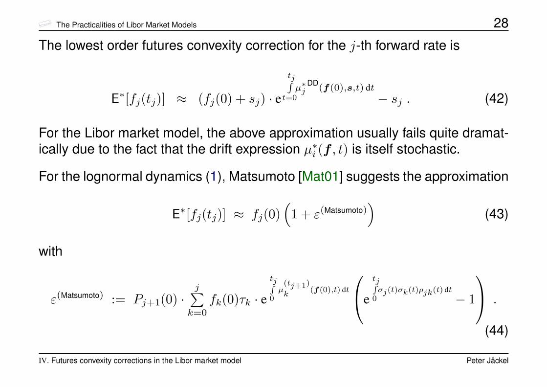
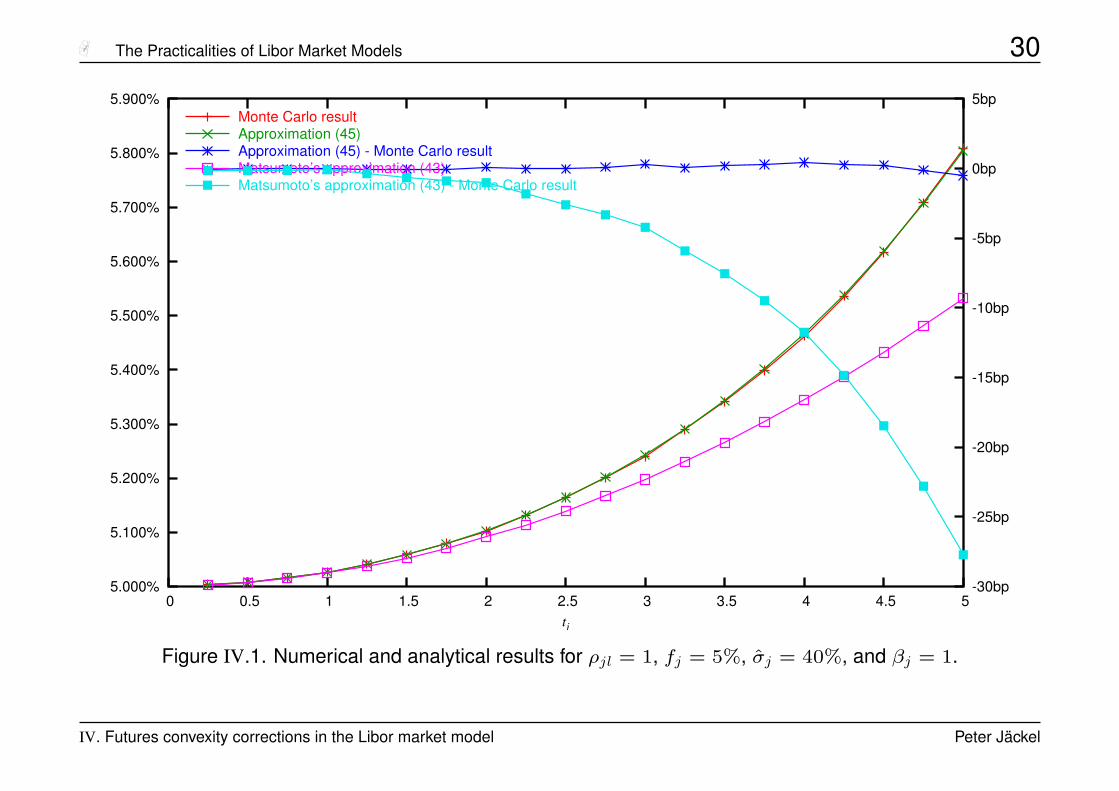
The lowest order futures convexity correction for the j-th forward rate is
E∗[fj(tj)] ≈ (fj(0) + sj) · e
tjRt=0µ∗j
DD(f(0),s,t) dt
− sj . (42)
For the Libor market model, the above approximation usually fails quite dramat-ically due to the fact that the drift expression µ∗i (f , t) is itself stochastic.
For the lognormal dynamics (1), Matsumoto [Mat01] suggests the approximation
E∗[fj(tj)] ≈ fj(0)(
1 + ε(Matsumoto))
(43)
with
ε(Matsumoto) := Pj+1(0) ·j∑
k=0
fk(0)τk · etjR0µ
(tj+1)
k(f(0),t) dt
e
tjR0σj(t)σk(t)ρjk(t) dt
− 1
.
(44)
IV. Futures convexity corrections in the Libor market model Peter Jäckel
The Practicalities of Libor Market Models 29
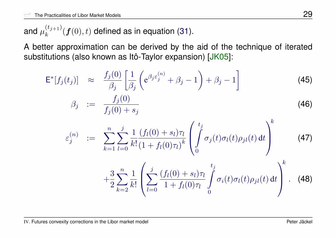
and µ(tj+1)
k (f(0), t) defined as in equation (31).
A better approximation can be derived by the aid of the technique of iteratedsubstitutions (also known as Itô-Taylor expansion) [JK05]:
E∗[fj(tj)] ≈ fj(0)βj
[1βj
(eβjε
(n)j + βj − 1
)+ βj − 1
](45)
βj :=fj(0)
fj(0) + sj(46)
ε(n)j :=
n∑k=1
j∑l=0
1k!
(fl(0) + sl)τl(1 + fl(0)τl)
k
tj∫0
σj(t)σl(t)ρjl(t) dt
k
(47)
+32
n∑k=2
1k!
j∑l=0
(fl(0) + sl)τl1 + fl(0)τl
tj∫0
σi(t)σl(t)ρjl(t) dt
k
. (48)
IV. Futures convexity corrections in the Libor market model Peter Jäckel
The Practicalities of Libor Market Models 30
5.000%
5.100%
5.200%
5.300%
5.400%
5.500%
5.600%
5.700%
5.800%
5.900%
0 0.5 1 1.5 2 2.5 3 3.5 4 4.5 5-30bp
-25bp
-20bp
-15bp
-10bp
-5bp
0bp
5bp
tj
Monte Carlo resultApproximation (45)Approximation (45) - Monte Carlo resultMatsumoto’s approximation (43)Matsumoto’s approximation (43) - Monte Carlo result
Figure IV.1. Numerical and analytical results for ρjl = 1, fj = 5%, σj = 40%, and βj = 1.
IV. Futures convexity corrections in the Libor market model Peter Jäckel

The Practicalities of Libor Market Models 31
5.000%
5.100%
5.200%
5.300%
5.400%
5.500%
5.600%
0 0.5 1 1.5 2 2.5 3 3.5 4 4.5 5-0.1bp
-0.05bp
0bp
0.05bp
0.1bp
0.15bp
0.2bp
0.25bp
0.3bp
tj
Monte Carlo resultApproximation (45)Approximation (45) - Monte Carlo result
Figure IV.2. Numerical and analytical results for ρjl = 1, fj = 5%, σj = 40%, and βj = 1/2.
IV. Futures convexity corrections in the Libor market model Peter Jäckel
The Practicalities of Libor Market Models 32
5.000%
5.100%
5.200%
5.300%
5.400%
5.500%
5.600%
0 0.5 1 1.5 2 2.5 3 3.5 4 4.5 5-0.2bp
-0.1bp
0bp
0.1bp
0.2bp
0.3bp
0.4bp
0.5bp
tj
Monte Carlo resultApproximation (45)Approximation (45) - Monte Carlo resultKirikos Novak formula (Hull-White model, fit at the money)Kirikos Novak formula (Hull-White model, fit at the money) - Monte Carlo result
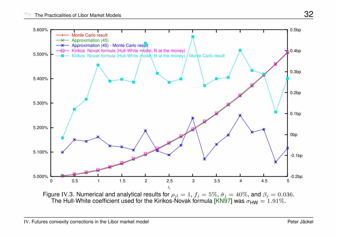
Figure IV.3. Numerical and analytical results for ρjl = 1, fj = 5%, σj = 40%, and βj = 0.036.The Hull-White coefficient used for the Kirikos-Novak formula [KN97] was σHW = 1.91%.
IV. Futures convexity corrections in the Libor market model Peter Jäckel

The Practicalities of Libor Market Models 33
1.000%
1.020%
1.040%
1.060%
1.080%
1.100%
1.120%
0 0.5 1 1.5 2 2.5 3 3.5 4 4.5 5-1.4bp
-1.2bp
-1bp
-0.8bp
-0.6bp
-0.4bp
-0.2bp
0bp
0.2bp
tj
Monte Carlo resultApproximation (45)Approximation (45) - Monte Carlo resultMatsumoto’s approximation (43)Matsumoto’s approximation (43) - Monte Carlo result
Figure IV.4. Numerical and analytical results for ρjl = 1, fj = 1%, σj = 60%, and βj = 1.
IV. Futures convexity corrections in the Libor market model Peter Jäckel
The Practicalities of Libor Market Models 34
1.000%
1.010%
1.020%
1.030%
1.040%
1.050%
1.060%
0 0.5 1 1.5 2 2.5 3 3.5 4 4.5 5-0.015bp
-0.01bp
-0.005bp
0bp
0.005bp
0.01bp
0.015bp
0.02bp
0.025bp
0.03bp
0.035bp
tj
Monte Carlo resultApproximation (45)Approximation (45) - Monte Carlo result
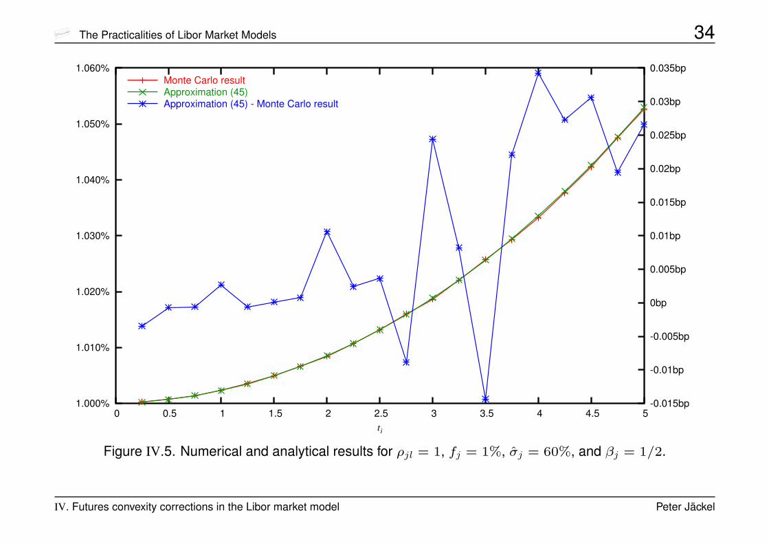
Figure IV.5. Numerical and analytical results for ρjl = 1, fj = 1%, σj = 60%, and βj = 1/2.
IV. Futures convexity corrections in the Libor market model Peter Jäckel
The Practicalities of Libor Market Models 35
1.000%
1.005%
1.010%
1.015%
1.020%
1.025%
1.030%
1.035%
1.040%
1.045%
0 0.5 1 1.5 2 2.5 3 3.5 4 4.5 5-0.18bp
-0.16bp
-0.14bp
-0.12bp
-0.1bp
-0.08bp
-0.06bp
-0.04bp
-0.02bp
0bp
0.02bp
tj
Monte Carlo resultApproximation (45)Approximation (45) - Monte Carlo resultKirikos Novak formula (Hull-White model, fit at the money)Kirikos Novak formula (Hull-White model, fit at the money) - Monte Carlo result
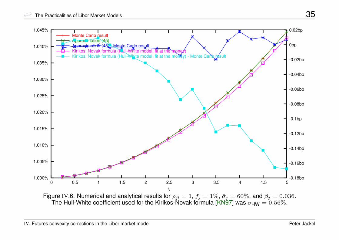
Figure IV.6. Numerical and analytical results for ρjl = 1, fj = 1%, σj = 60%, and βj = 0.036.The Hull-White coefficient used for the Kirikos-Novak formula [KN97] was σHW = 0.56%.
IV. Futures convexity corrections in the Libor market model Peter Jäckel
The Practicalities of Libor Market Models 36
5.000%
5.100%
5.200%
5.300%
5.400%
5.500%
5.600%
0 0.5 1 1.5 2 2.5 3 3.5 4 4.5 5-18bp
-16bp
-14bp
-12bp
-10bp
-8bp
-6bp
-4bp
-2bp
0bp
2bp
tj
Monte Carlo resultApproximation (45)Approximation (45) - Monte Carlo resultMatsumoto’s approximation (43)Matsumoto’s approximation (43) - Monte Carlo result
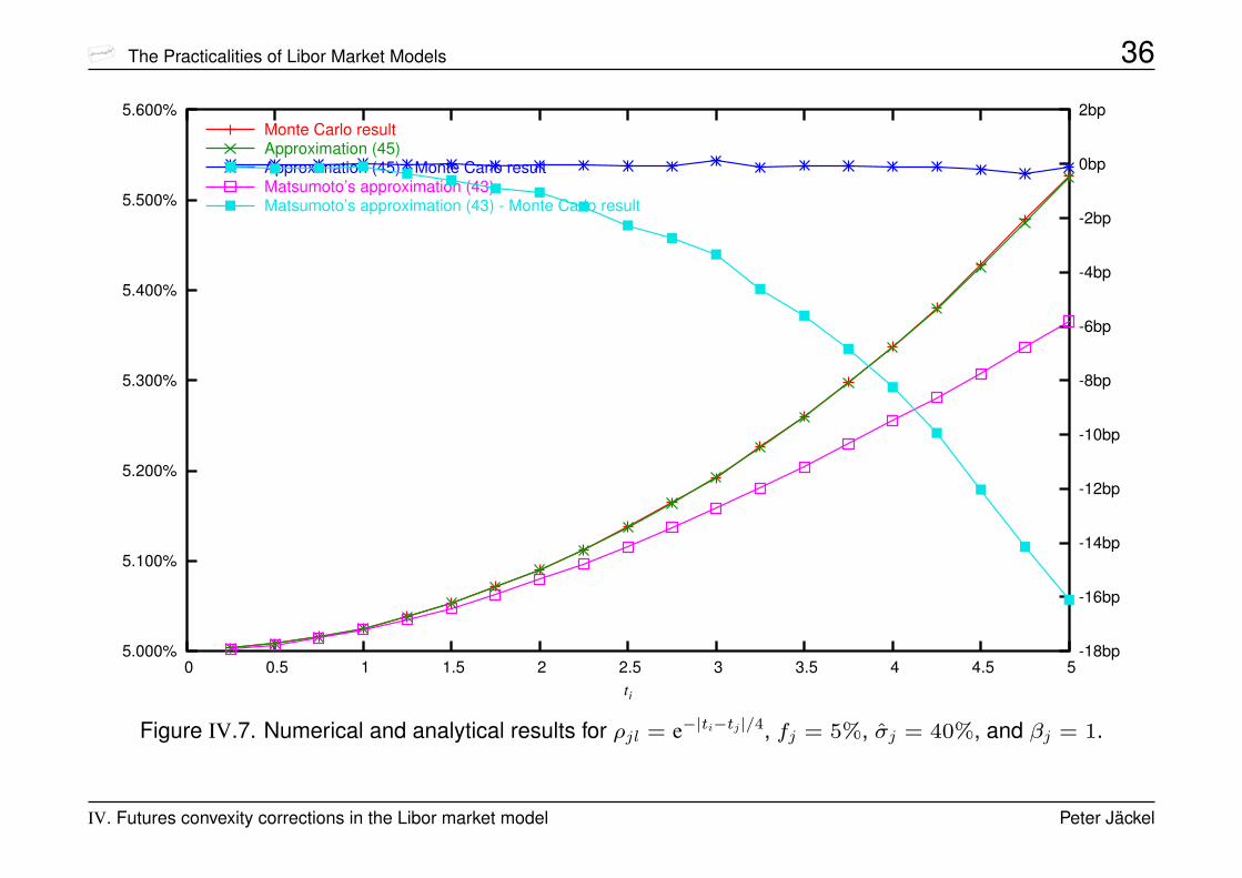
Figure IV.7. Numerical and analytical results for ρjl = e−|ti−tj|/4, fj = 5%, σj = 40%, and βj = 1.
IV. Futures convexity corrections in the Libor market model Peter Jäckel
The Practicalities of Libor Market Models 37
5.000%
5.050%
5.100%
5.150%
5.200%
5.250%
5.300%
5.350%
5.400%
0 0.5 1 1.5 2 2.5 3 3.5 4 4.5 5-0.1bp
-0.05bp
0bp
0.05bp
0.1bp
0.15bp
0.2bp
tj
Monte Carlo resultApproximation (45)Approximation (45) - Monte Carlo result
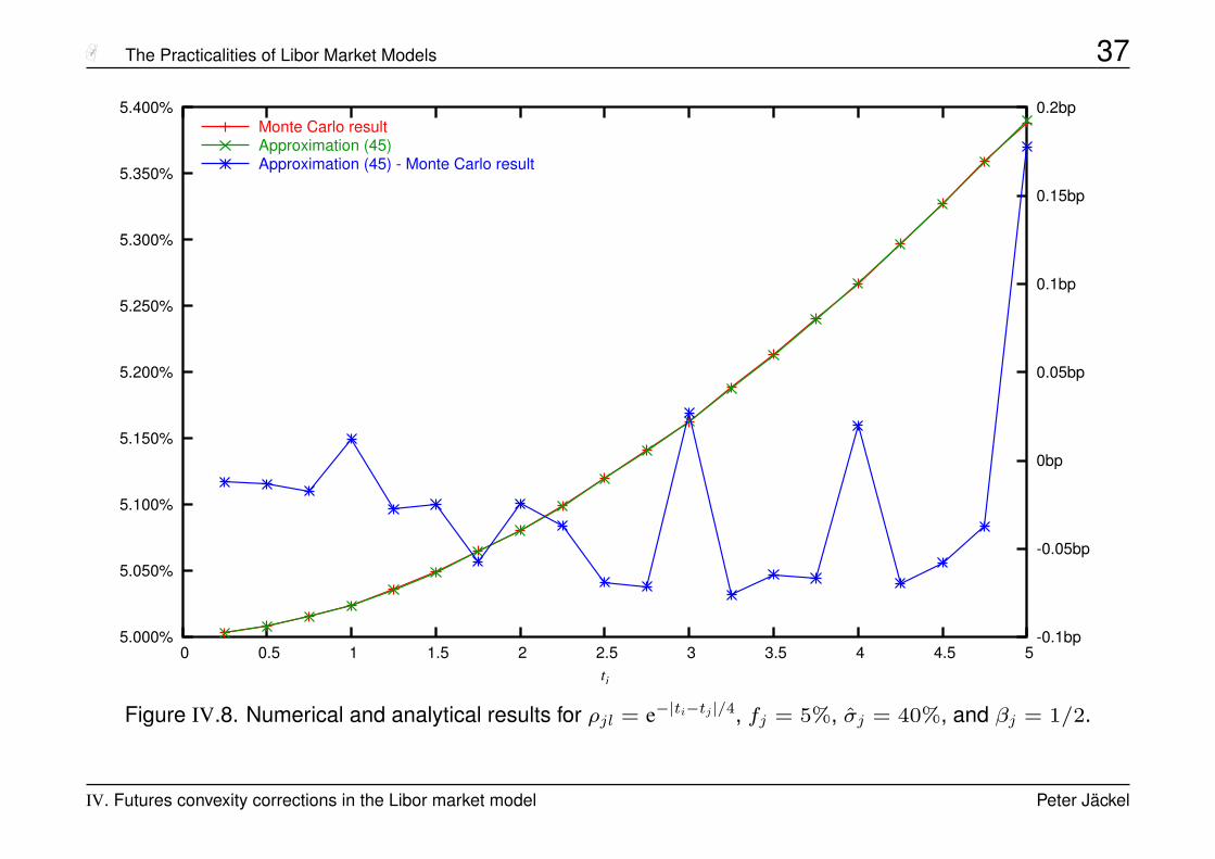
Figure IV.8. Numerical and analytical results for ρjl = e−|ti−tj|/4, fj = 5%, σj = 40%, and βj = 1/2.
IV. Futures convexity corrections in the Libor market model Peter Jäckel
The Practicalities of Libor Market Models 38
5.000%
5.050%
5.100%
5.150%
5.200%
5.250%
5.300%
5.350%
5.400%
0 0.5 1 1.5 2 2.5 3 3.5 4 4.5 5-0.15bp
-0.1bp
-0.05bp
0bp
0.05bp
0.1bp
tj
Monte Carlo resultApproximation (45)Approximation (45) - Monte Carlo result
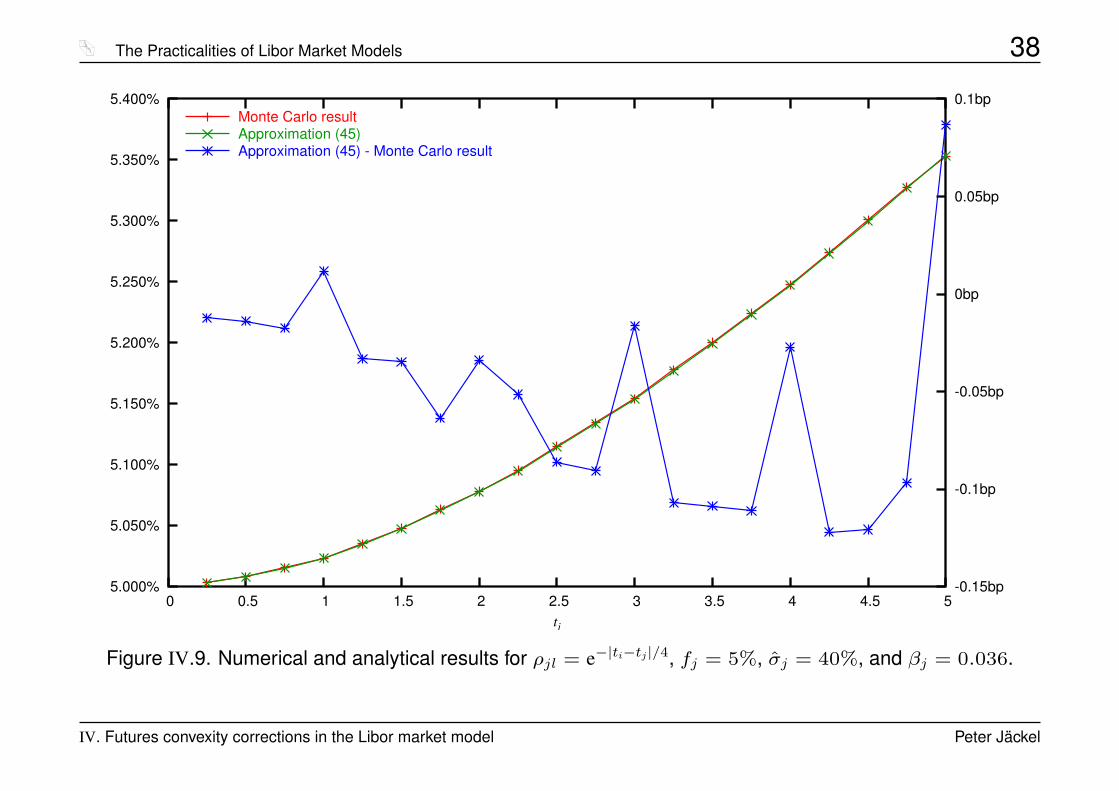
Figure IV.9. Numerical and analytical results for ρjl = e−|ti−tj|/4, fj = 5%, σj = 40%, and βj = 0.036.
IV. Futures convexity corrections in the Libor market model Peter Jäckel

The Practicalities of Libor Market Models 39
V. Speed is everything — the predictor-corrector scheme
In order to price an exotic interest rate derivative, we need to evolve the set offorward rates f from its present values into the future.
The drift terms given by equation (41) are clearly state-dependent and thus in-directly stochastic which forces us to use a numerical scheme to solve equation(40) along any one path.
A simple explicit Euler scheme for the state variables xi := fi + si is
xEuleri (t+ ∆t) = xi(t) + xi(t) · µi(t)∆t + xi(t) ·
m∑j=1
aij(t)zj√
∆t (49)
with zj being m independent normal variates.
This would imply that we approximate the drift and volatilities as constant overthe time step t → t + ∆t, not even taking into account any term structure ofvolatility.
V. Speed is everything — the predictor-corrector scheme Peter Jäckel

The Practicalities of Libor Market Models 40
Moreover, this scheme effectively means that we are using a normal distributionfor the evolution of the forward rates over this time step.
Whilst we may agree to the approximation of a piecewise constant (in time)drift coefficient µi, the normal distribution may be undesirable, especially if weenvisage to use large time steps ∆t for reasons of computational efficiency.
However, when we assume piecewise constant drift, we might as well carry outthe integration over the time step ∆t analytically and use the scheme
xConstant drifti (f(t), t+ ∆t) = xi(t) · e
µi(f(t),t)∆t−12 cii+
mPj=1
aijzj(50)
with
cij =
t+∆t∫t
σi(u)σj(u)ρij(u) du (51)
V. Speed is everything — the predictor-corrector scheme Peter Jäckel

The Practicalities of Libor Market Models 41
and A being the spectral square root3 of C:
C = A · A> . (52)
This is essentially an Euler scheme in logarithmic coordinates.
The above procedure works very well as long as the time steps ∆t are not toolong and is widely used and also referred to in publications [And00, GZ99].
Since the drift term appearing in the exponential function in equation (50) isin some sense a stochastic quantity itself, we will begin to notice that we areignoring Jensen’s inequality when the term µi∆t becomes large enough.
This happens when we choose a big step ∆t, or the forward rates themselvesor their volatility are large. Therefore, we should use a hybrid predictor-correctormethod which models only the drift as indirectly stochastic.
A method that works very well in practice is as follows.3also known as Schur decomposition
V. Speed is everything — the predictor-corrector scheme Peter Jäckel

The Practicalities of Libor Market Models 42
1. Given a current evolution of the yield curve denoted by x(t), we calculate thepredicted solution xConstant drift(x(t), t + ∆t) using one m-dimensional normalvariate draw z following equation (50).
2. We recalculate the drift using this evolved yield curve. The predictor-correctorapproximation µi for the drift is then given by the average of these two calcu-lated drifts, i.e.
µi(x(t), t → t+ ∆t) = 1/2{µi(x(t), t) (53)
+ µi(xConstant drift(x(t), t+ ∆t), t)}.
3. The predictor-corrector evolution is given by
xPredictor-correctori (x(t), t+ ∆t) = xi(t) · e
µi(x(t),t→ t+∆t)∆t−12 cii+
mPj=1
aijzj(54)
wherein we re-use the same normal variate draw z, i.e. we only correct thedrift of the predicted solution.
V. Speed is everything — the predictor-corrector scheme Peter Jäckel

The Practicalities of Libor Market Models 43����������� ������������������������������
������� ��������"!$#%�'&()! ττττ �*���,+"-��
.�/10324/15
/$0 /"/$5
/$0326/$5
/$0376/$5
/$0386/$5
/$0 9"/$5
/$03:6/$5
;�< =?>�< =?;�< @�>�< @�;�< A�>B< A�;B< CB>�<
DBEGF$H�I J�K�LBM�H N�O?I3H�I OQP
RS TUV WX YYZZUZ[ \]^ _` \UXa[ TbUW\X Yac
dfe?gihkj�l%gij�m?npo qrjs n�tum?o vQj�eunpwpv6eunpnpt%v6j3e?nxfy{z v6l%|?} t%j�~�t%�il
������������� ������� �������������� �����σσσσ����� �"!$#%� &�"! ττττ �(' ��)+*��
,.-�/102-%3
-�/ -4-43
-�/502-43
-�/ 64-43
-�/ 74-43
-�/ 84-43
-�/ 94-43
- 9 02- 029 64- 649 74- 7%9 84- 849 94-
:%;�<�=1>@?BA.?DC�E�>GF%H
IJ KLM NO PPQQLQR STU VW SLOXR KYLNSO PXZ
[$\�]�^`_bac]d_e�f`g h _i f`jke�g lm_b\�fmn`ld\�f`fmjklo_b\cfp$q�r ldaks�t j�_vu�jcw�a
Figure V.1. The stability of the predictor-corrector drift method as a function of volatility level(left) and time to expiry (right) for the Libor-in-arrears convexity.
Ü The predictor-corrector drift approximation is highly accurate!
V. Speed is everything — the predictor-corrector scheme Peter Jäckel

The Practicalities of Libor Market Models 44
VI. Parametrisation of correlation and volatility backbone
Stable calibration of any market model relies on the specification of a robust yetflexible reference volatility structure. We call a specification of instantaneousvolatility time-homogeneous or stationary if the volatility of any forward rate fTthat will fix at time T depends on calendar time t only in terms of T − t, i.e.
σT (t) = σ(T − t) . (55)
One cannot fit many market prices with this strict assumption.
In fact, there are frequently good economic reasons why time-homogeneity maynot be given for the term structure of instantaneous volatility of forward rates.
In practice, we may want to use an initial parametrised fit in order to find thevalues a, b, c, and d, such that (only) the caplet implied volatilities resulting fromthe instantaneous FRA volatility
σi(t) = ki
[(a+ b · (ti − t)) · e−c·(ti−t) + d
]· 1{t<ti} (56)
VI. Parametrisation of correlation and volatility backbone Peter Jäckel
The Practicalities of Libor Market Models 45
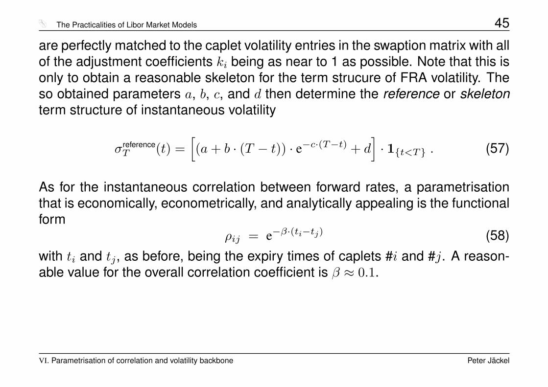
are perfectly matched to the caplet volatility entries in the swaption matrix with allof the adjustment coefficients ki being as near to 1 as possible. Note that this isonly to obtain a reasonable skeleton for the term strucure of FRA volatility. Theso obtained parameters a, b, c, and d then determine the reference or skeletonterm structure of instantaneous volatility
σreferenceT (t) =
[(a+ b · (T − t)) · e−c·(T−t) + d
]· 1{t<T} . (57)
As for the instantaneous correlation between forward rates, a parametrisationthat is economically, econometrically, and analytically appealing is the functionalform
ρij = e−β·(ti−tj) (58)with ti and tj, as before, being the expiry times of caplets #i and #j. A reason-able value for the overall correlation coefficient is β ≈ 0.1.
VI. Parametrisation of correlation and volatility backbone Peter Jäckel
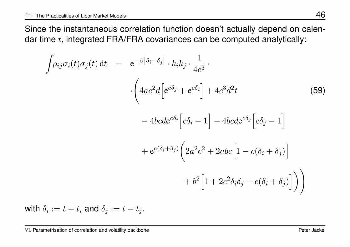
The Practicalities of Libor Market Models 46
Since the instantaneous correlation function doesn’t actually depend on calen-dar time t, integrated FRA/FRA covariances can be computed analytically:∫
ρijσi(t)σj(t) dt = e−β|δi−δj| · kikj ·1
4c3·
·
(4ac2d
[ecδj + ecδi
]+ 4c3d2t (59)
− 4bcdecδi[cδi − 1
]− 4bcdecδj
[cδj − 1
]+ ec(δi+δj)
(2a2c2 + 2abc
[1− c(δi + δj)
]+ b2
[1 + 2c2δiδj − c(δi + δj)
]))
with δi := t− ti and δj := t− tj.
VI. Parametrisation of correlation and volatility backbone Peter Jäckel

The Practicalities of Libor Market Models 47
The quality of a reference fit of the implied volatilities consistent with equation(56) for a typical yield curve and caplet market both in EUR and USD is usuallyquite good:
Figure VI.1.
�����������
���
���
���
���
���
���
���
��
��
� � � � � � � � ��
���� �������
� ������������������������
� ����������� �!��"�������#����������$�%��
&'�����������������������
&'���������� �!��"�������#����������$�%��
VI. Parametrisation of correlation and volatility backbone Peter Jäckel
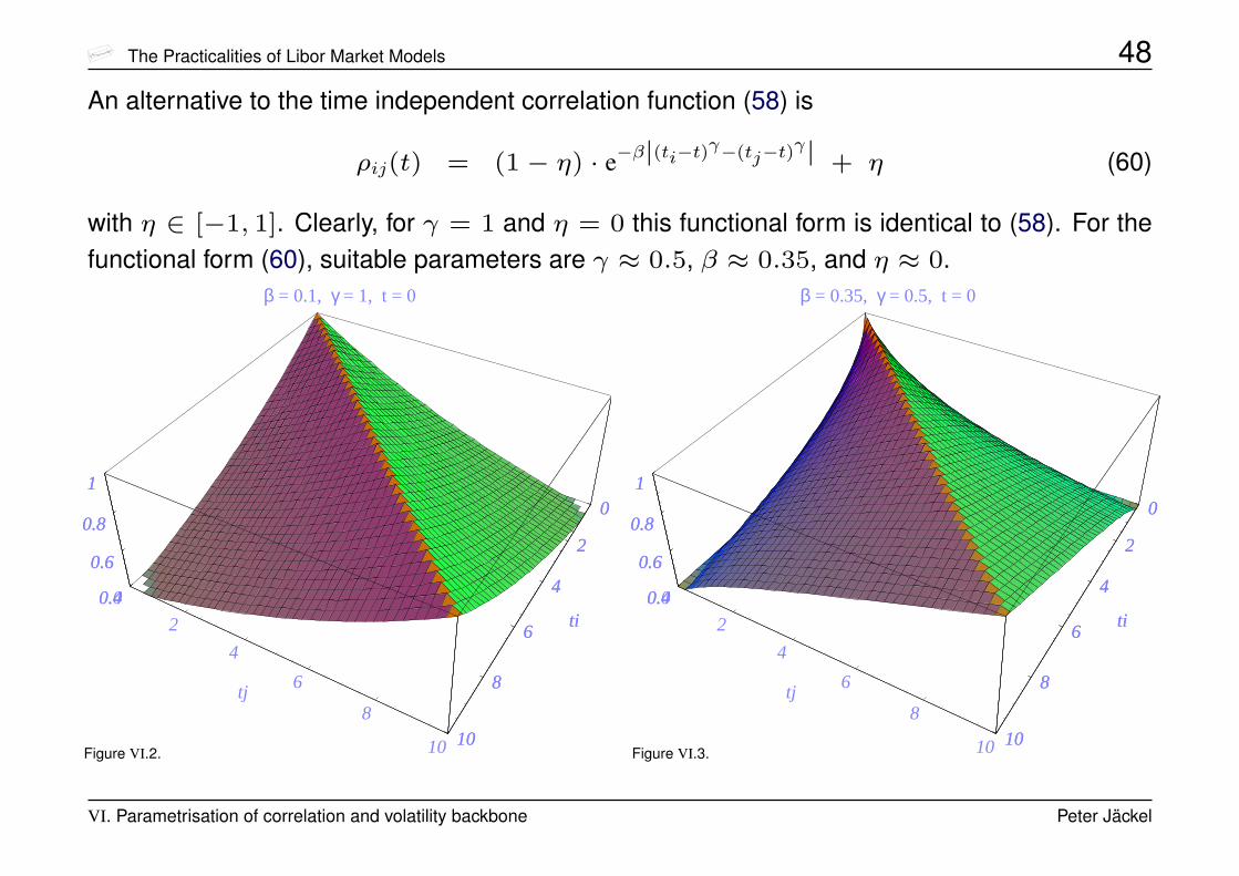
The Practicalities of Libor Market Models 48An alternative to the time independent correlation function (58) is
ρij(t) = (1− η) · e−β|(ti−t)γ−(tj−t)
γ| + η (60)
with η ∈ [−1, 1]. Clearly, for γ = 1 and η = 0 this functional form is identical to (58). For thefunctional form (60), suitable parameters are γ ≈ 0.5, β ≈ 0.35, and η ≈ 0.
Figure VI.2.
β = 0.1, γ = 1, t = 0
0
2
4
6
8
10
ti0
2
4
6
8
10
tj
0.4
0.6
0.8
10
2
4
6
8
10
ti0.4
0.6
0.8
1
Figure VI.3.
β = 0.35, γ = 0.5, t = 0
0
2
4
6
8
10
ti0
2
4
6
8
10
tj
0.4
0.6
0.8
10
2
4
6
8
10
ti0.4
0.6
0.8
1
VI. Parametrisation of correlation and volatility backbone Peter Jäckel
The Practicalities of Libor Market Models 49
VII. Factor reduction — pros and cons
It is possible to drive the evolution of the n forward rates with fewer underlyingindependent standard Wiener processes than there are forward rates, say onlym of them.
In this case, the coefficient matrix A ∈ Rn×n is to be replaced by A ∈ Rn×m
which must satisfym∑k=1
a2jk = cjj (61)
in order to retain the calibration of the options on the FRAs, i.e. the caplets.
In practice, this can be done very easily by calculating the decomposition as inequation (4) as before and rescaling according to
ajk → ajk
√cjjm∑l=1
a2jl
. (62)
VII. Factor reduction — pros and cons Peter Jäckel

The Practicalities of Libor Market Models 50
The effect of this procedure is that the individual variances of each of the ratesare still correct, even if we have reduced the number of driving factors to one,but the effective covariances will differ.
However, if we allow for a term structure of volatility, or loading coefficients ajk,factor reduction disables us from taking time steps longer than our time discreti-sation.
For example, assuming piecewise constant instantaneous loading coefficientsfor two factors of four forward rates over a first semi-annual time step
A1 =( 0.259 0.104
0.245 0.0170.214 −0.0660.177 −0.096
)→ C1 = A1 ·A>1 =
(0.078 0.065 0.049 0.0360.065 0.060 0.051 0.0420.049 0.051 0.050 0.0440.036 0.042 0.044 0.040
)(63)
and over a second semi-annual time step
A2 =( 0.280 0.122
0.282 0.0370.264 −0.0660.232 −0.118
)→ C2 = A2 ·A>2 =
(0.094 0.084 0.066 0.0510.084 0.081 0.072 0.0610.066 0.072 0.074 0.0690.051 0.061 0.069 0.067
)(64)
VII. Factor reduction — pros and cons Peter Jäckel
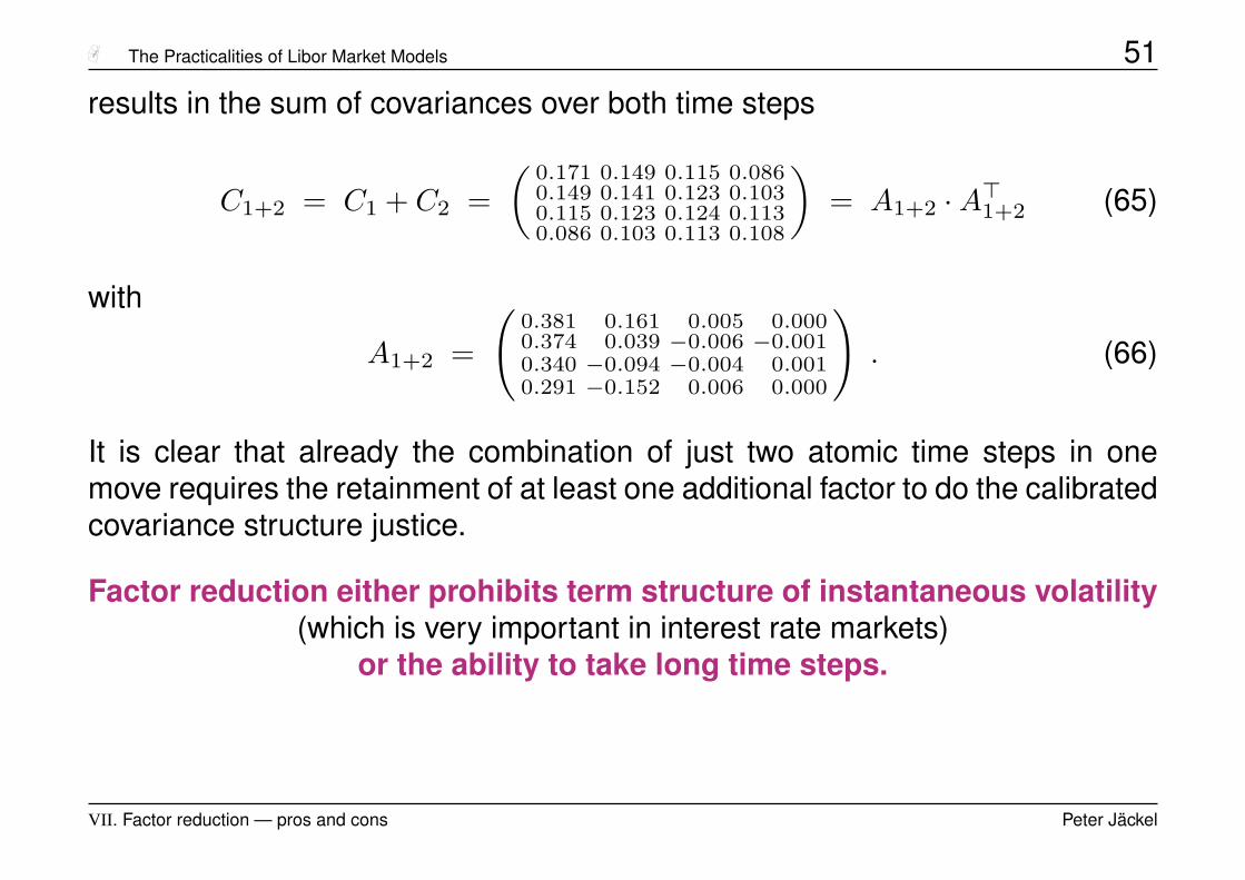
The Practicalities of Libor Market Models 51
results in the sum of covariances over both time steps
C1+2 = C1 + C2 =(
0.171 0.149 0.115 0.0860.149 0.141 0.123 0.1030.115 0.123 0.124 0.1130.086 0.103 0.113 0.108
)= A1+2 ·A>1+2 (65)
with
A1+2 =
(0.381 0.161 0.005 0.0000.374 0.039 −0.006 −0.0010.340 −0.094 −0.004 0.0010.291 −0.152 0.006 0.000
). (66)
It is clear that already the combination of just two atomic time steps in onemove requires the retainment of at least one additional factor to do the calibratedcovariance structure justice.
Factor reduction either prohibits term structure of instantaneous volatility(which is very important in interest rate markets)
or the ability to take long time steps.
VII. Factor reduction — pros and cons Peter Jäckel
The Practicalities of Libor Market Models 52
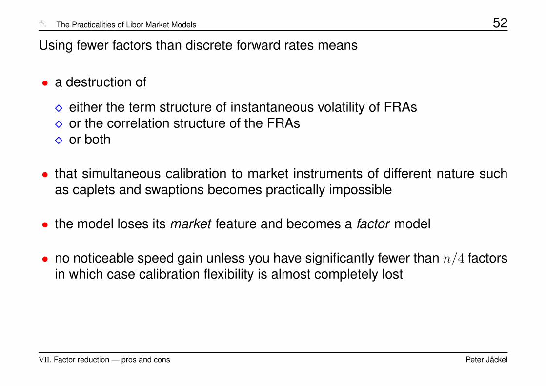
Using fewer factors than discrete forward rates means
• a destruction of
� either the term structure of instantaneous volatility of FRAs� or the correlation structure of the FRAs� or both
• that simultaneous calibration to market instruments of different nature suchas caplets and swaptions becomes practically impossible
• the model loses its market feature and becomes a factor model
• no noticeable speed gain unless you have significantly fewer than n/4 factorsin which case calibration flexibility is almost completely lost
VII. Factor reduction — pros and cons Peter Jäckel

The Practicalities of Libor Market Models 53
VIII. Speed is everything — the drift term
If we wish to run a Libor market model with deterministic volatilities in the spotLibor measure with m factors, expediency commands that we precompute all ofthe terms
cijk :=∫ ti+1
ti
σDDj (t)ρjk(t)σDD
k (t) dt (67)
and the spectral split matrices Ai such that
cijk =m∑l=1
aijkaijl (68)
i.e.Ci = Ai · A>i . (69)
VIII. Speed is everything — the drift term Peter Jäckel
The Practicalities of Libor Market Models 54
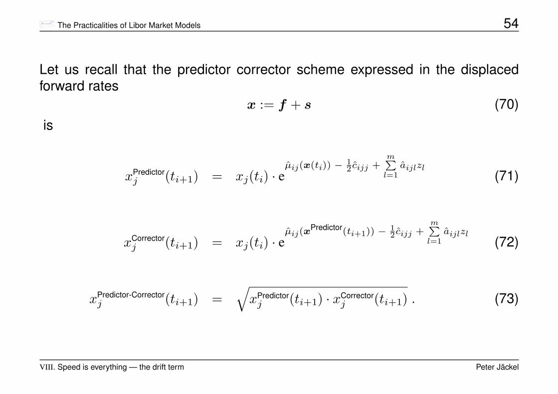
Let us recall that the predictor corrector scheme expressed in the displacedforward rates
x := f + s (70)is
xPredictorj (ti+1) = xj(ti) · e
µij(x(ti)) − 12 cijj +
mPl=1
aijlzl(71)
xCorrectorj (ti+1) = xj(ti) · e
µij(xPredictor(ti+1)) − 1
2 cijj +mPl=1
aijlzl(72)
xPredictor-Correctorj (ti+1) =
√xPredictorj (ti+1) · xCorrector
j (ti+1) . (73)
VIII. Speed is everything — the drift term Peter Jäckel
The Practicalities of Libor Market Models 55
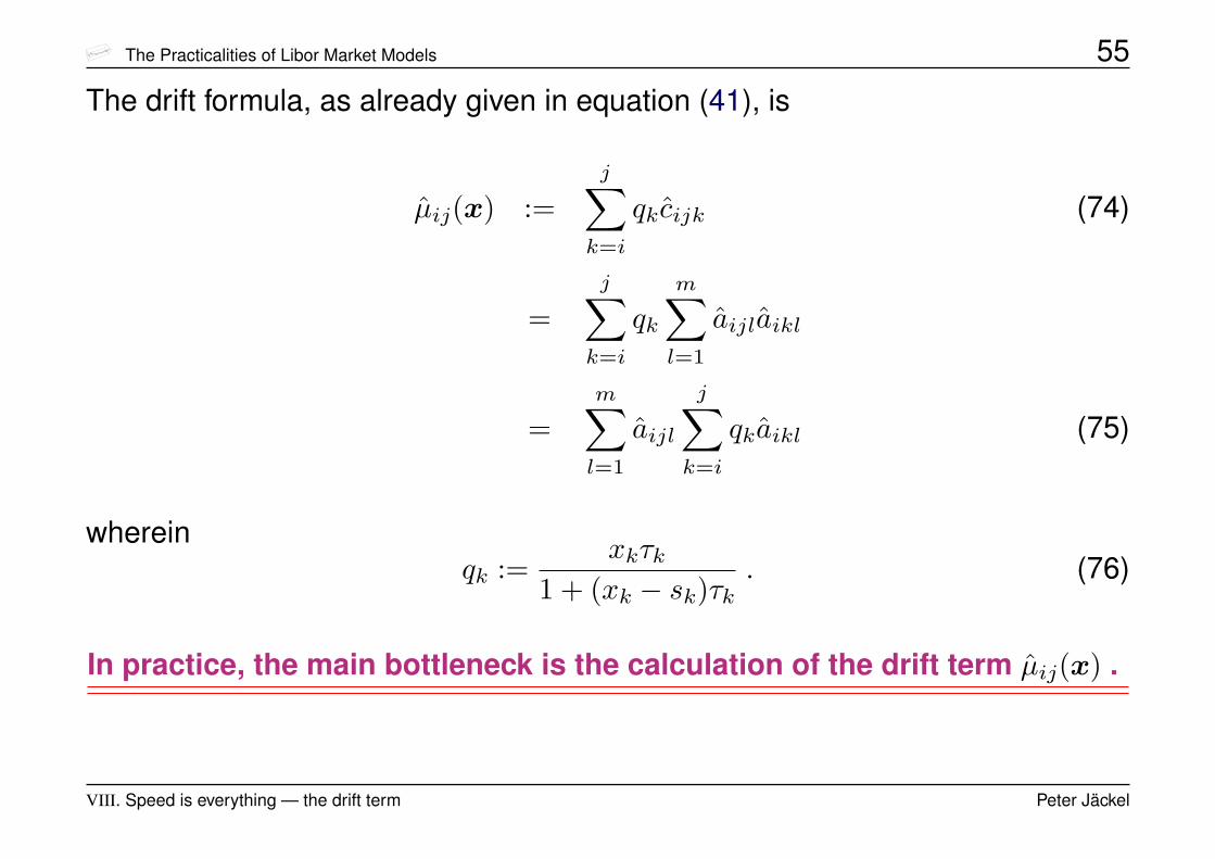
The drift formula, as already given in equation (41), is
µij(x) :=j∑k=i
qkcijk (74)
=j∑k=i
qk
m∑l=1
aijlaikl
=m∑l=1
aijl
j∑k=i
qkaikl (75)
whereinqk :=
xkτk1 + (xk − sk)τk
. (76)
In practice, the main bottleneck is the calculation of the drift term µij(x) .
VIII. Speed is everything — the drift term Peter Jäckel

The Practicalities of Libor Market Models 56
At time ti, only n = N − i forward rates are alive.
Thus, for ti → ti+1, to compute all of the drift terms µij(x) for j = i . . . N , usingthe formula (74)
µij(x) =j∑k=i
qkcijk
involves
n(n+ 1)
2(77)
multiplications and additions4.
4assuming we have precomputed the coefficients qk from this vector x which we definitely must do (factor2 speedup!)
VIII. Speed is everything — the drift term Peter Jäckel

The Practicalities of Libor Market Models 57
For small m, the calculation of µij(x) for j = i . . . N , using the formula (75) as in
µij(x) =m∑l=1
aijlrijl (78)
with the update rulerijl = ri(j−1)l + qjaijl , (79)
which involves2nm (80)
multiplications and additions, can be advantageous5 if 2nm < n(n+1)2 , i.e. if
m ≤ n/4 . (81)
In practice, the alternative algorithm (78)-(79) is only helpfulin conjunction with extreme factor reduction.
5This recursive decomposition can be generalised for swap market models and other yield curve representa-tions [PvR05]
VIII. Speed is everything — the drift term Peter Jäckel
The Practicalities of Libor Market Models 58
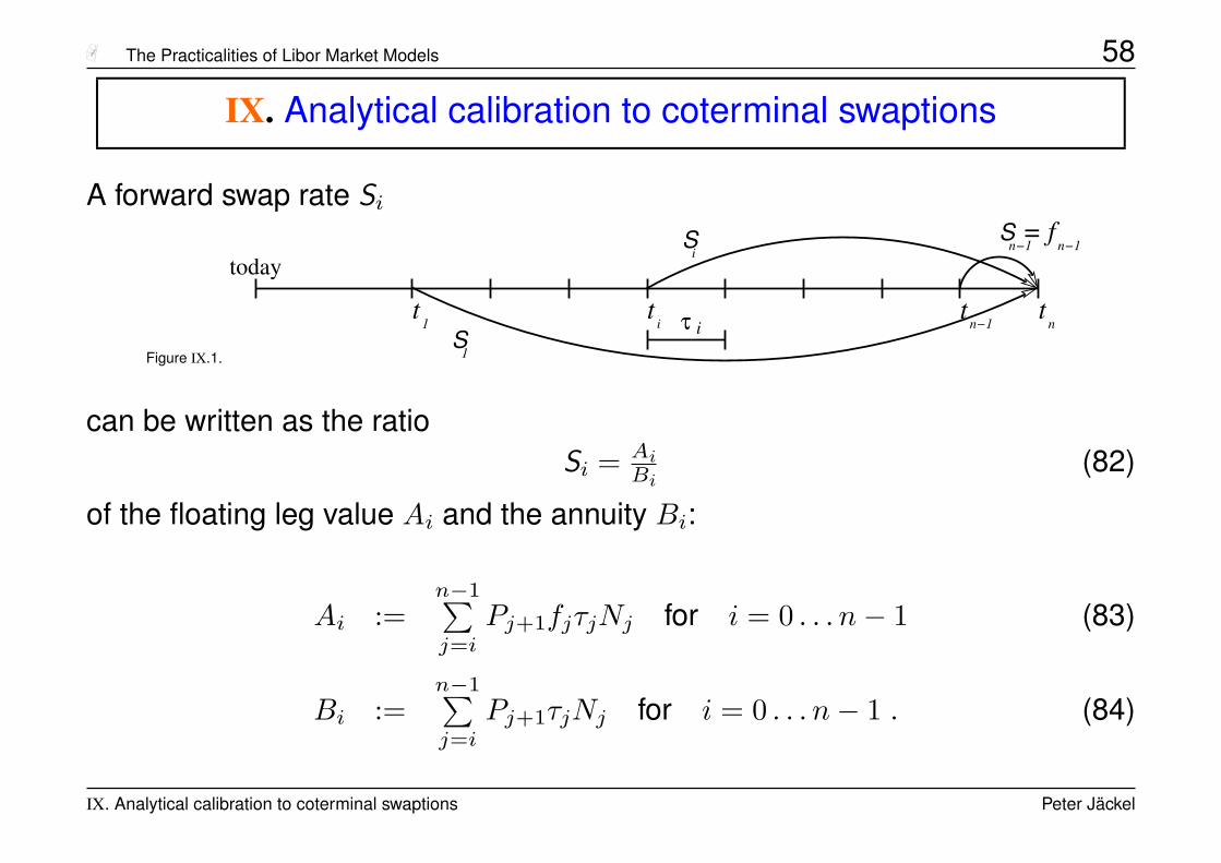
IX. Analytical calibration to coterminal swaptions
A forward swap rate Si
Figure IX.1.
iS
today
t1
t
fn−1
Sn−1
=
n−1S
1
tn
ti iτ
can be written as the ratioSi = Ai
Bi(82)
of the floating leg value Ai and the annuity Bi:
Ai :=n−1∑j=i
Pj+1fjτjNj for i = 0 . . . n− 1 (83)
Bi :=n−1∑j=i
Pj+1τjNj for i = 0 . . . n− 1 . (84)
IX. Analytical calibration to coterminal swaptions Peter Jäckel

The Practicalities of Libor Market Models 59Nj is the notional associated with accrual period τj.
IX. Analytical calibration to coterminal swaptions Peter Jäckel
The Practicalities of Libor Market Models 60
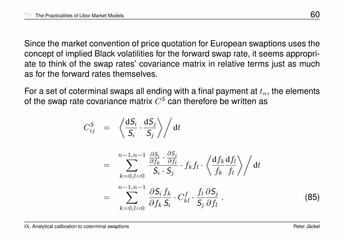
Since the market convention of price quotation for European swaptions uses theconcept of implied Black volatilities for the forward swap rate, it seems appropri-ate to think of the swap rates’ covariance matrix in relative terms just as muchas for the forward rates themselves.
For a set of coterminal swaps all ending with a final payment at tn, the elementsof the swap rate covariance matrix CS can therefore be written as
CSij =
⟨dSiSi· dSj
Sj
⟩/dt
=n−1,n−1∑k=0,l=0
∂Si∂fk· ∂Sj∂fl
Si · Sj· fkfl ·
⟨dfkfk
dflfl
⟩/dt
=n−1,n−1∑k=0,l=0
∂Si∂fk
fkSi· Cfkl ·
flSj
∂Sj∂fl
. (85)
IX. Analytical calibration to coterminal swaptions Peter Jäckel
The Practicalities of Libor Market Models 61
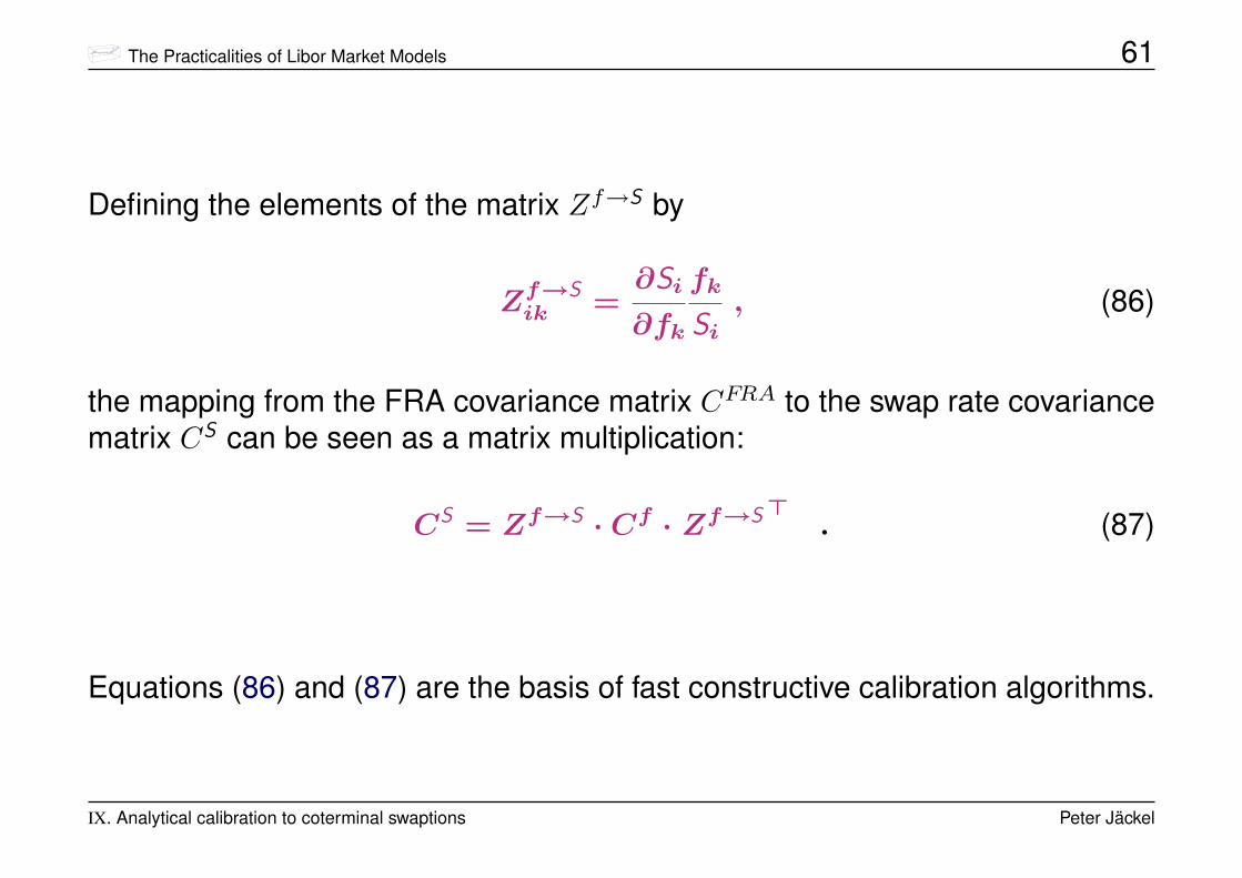
Defining the elements of the matrix Zf→S by
Zf→Sik =
∂Si
∂fk
fk
Si, (86)
the mapping from the FRA covariance matrix CFRA to the swap rate covariancematrix CS can be seen as a matrix multiplication:
CS = Zf→S · Cf · Zf→S >. (87)
Equations (86) and (87) are the basis of fast constructive calibration algorithms.
IX. Analytical calibration to coterminal swaptions Peter Jäckel
The Practicalities of Libor Market Models 62
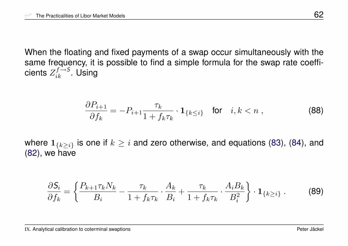
When the floating and fixed payments of a swap occur simultaneously with thesame frequency, it is possible to find a simple formula for the swap rate coeffi-cients Zf→S
ik . Using
∂Pi+1
∂fk= −Pi+1
τk1 + fkτk
· 1{k≤i} for i, k < n , (88)
where 1{k≥i} is one if k ≥ i and zero otherwise, and equations (83), (84), and(82), we have
∂Si∂fk
={Pk+1τkNk
Bi− τk
1 + fkτk· AkBi
+τk
1 + fkτk· AiBkB2i
}· 1{k≥i} . (89)
IX. Analytical calibration to coterminal swaptions Peter Jäckel
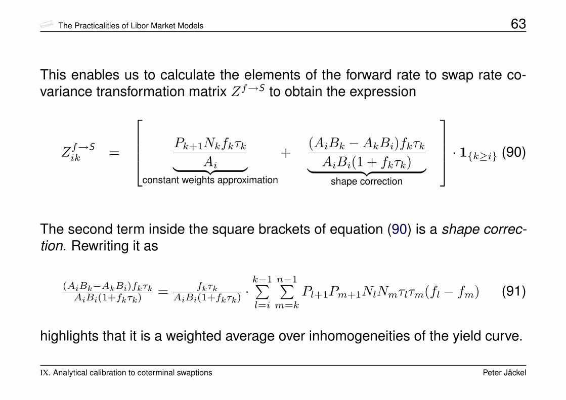
The Practicalities of Libor Market Models 63
This enables us to calculate the elements of the forward rate to swap rate co-variance transformation matrix Zf→S to obtain the expression
Zf→Sik =
Pk+1NkfkτkAi︸ ︷︷ ︸
constant weights approximation
+(AiBk −AkBi)fkτkAiBi(1 + fkτk)︸ ︷︷ ︸
shape correction
· 1{k≥i} .(90)
The second term inside the square brackets of equation (90) is a shape correc-tion. Rewriting it as
(AiBk−AkBi)fkτkAiBi(1+fkτk)
= fkτkAiBi(1+fkτk)
·k−1∑l=i
n−1∑m=k
Pl+1Pm+1NlNmτlτm(fl − fm) (91)
highlights that it is a weighted average over inhomogeneities of the yield curve.
IX. Analytical calibration to coterminal swaptions Peter Jäckel
The Practicalities of Libor Market Models 64
In fact, for a flat yield curve, all of the terms (fl−fm) are identically zero and themapping matrix Zf→s is equivalent to the so-called constant-weights approxi-mation.
In practice the yield curve is never entirely flat which makes it necessary tocompute the swap rate coefficients via the full derivative calculation (86).
When floating and fixed schedules differ, we have to compute the partial depen-dencies of the swap rates’ floating payments, floating payment discount factors,and fixed payment discount factors individually, but we still obtain a transforma-tion of the form (87), i.e
Cf → CS = Zf→S · Cf · Zf→S> .
IX. Analytical calibration to coterminal swaptions Peter Jäckel

The Practicalities of Libor Market Models 65
We now have a map between the instantaneous FRA/FRA covariance matrixand the instantaneous swap/swap covariance matrix.
Unfortunately, though, the map involves the state of the yield curve at any onegiven point in time via the matrix Z.
The price of a European swaption does not just depend on one single realisedstate or even path of instantaneous volatility. It is much more appropriate to thinkabout some kind of path integral average volatility.
Using arguments of factor decomposition and equal probability of up and downmoves (in logarithmic coordinates), it can be shown [JR00, Kaw02, Kaw03] thatthe specific structure of the map allows us to approximate the effective impliedswaption volatilities by simply using today’s state of the yield curve for the calcu-lation of the mapping matrix Z:
σSi(t, T ) =
√√√√ n−1∑k=i,l=i
Zf→sik (0) ·∫ Ttσk(t′)σl(t′)ρkl(t′)dt′
T − t· Zf→sil (0) (92)
IX. Analytical calibration to coterminal swaptions Peter Jäckel
The Practicalities of Libor Market Models 66
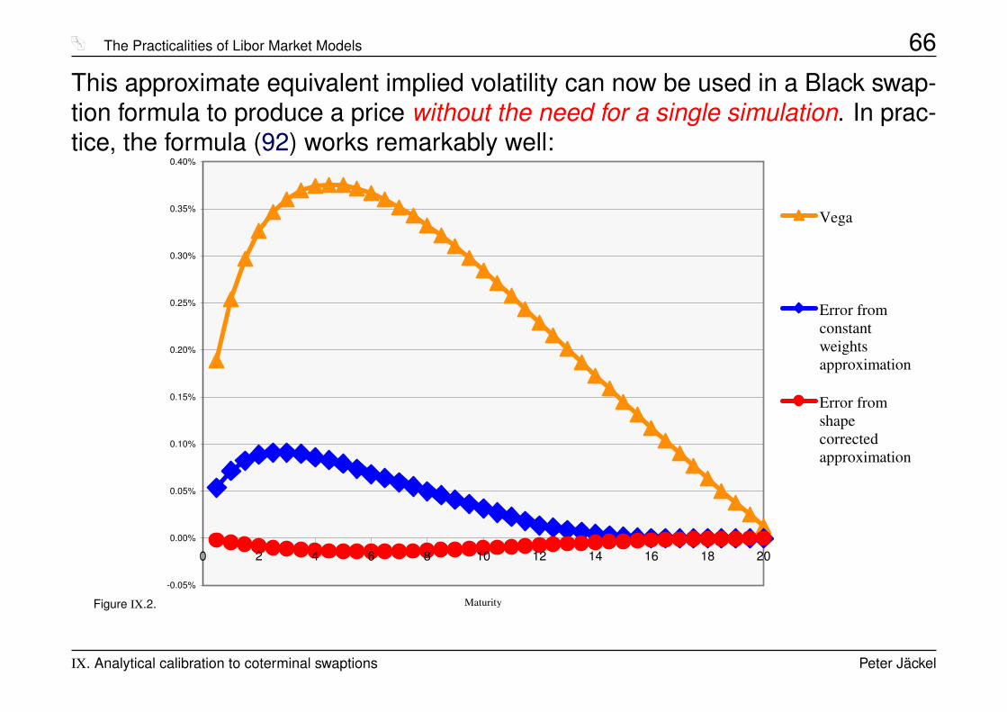
This approximate equivalent implied volatility can now be used in a Black swap-tion formula to produce a price without the need for a single simulation. In prac-tice, the formula (92) works remarkably well:
Figure IX.2.
-0.05%
0.00%
0.05%
0.10%
0.15%
0.20%
0.25%
0.30%
0.35%
0.40%
0 2 4 6 8 10 12 14 16 18 20
Maturity
Vega
Error fromconstantweightsapproximation
Error fromshapecorrectedapproximation
IX. Analytical calibration to coterminal swaptions Peter Jäckel
The Practicalities of Libor Market Models 67
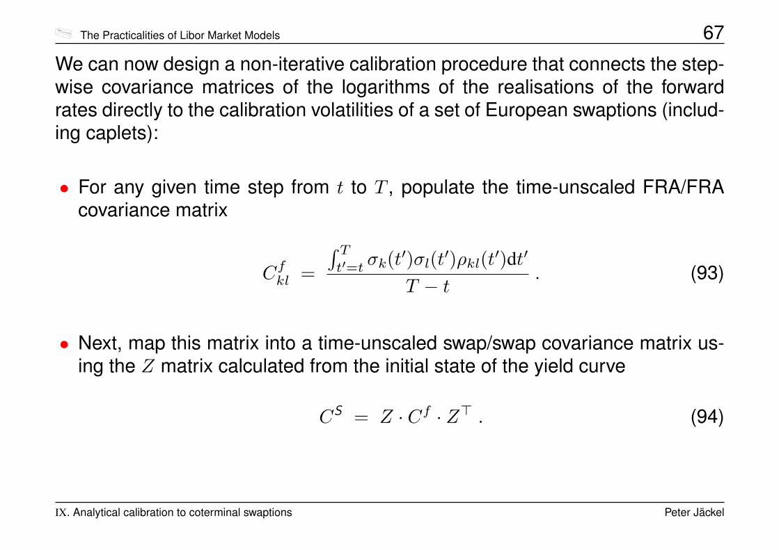
We can now design a non-iterative calibration procedure that connects the step-wise covariance matrices of the logarithms of the realisations of the forwardrates directly to the calibration volatilities of a set of European swaptions (includ-ing caplets):
• For any given time step from t to T , populate the time-unscaled FRA/FRAcovariance matrix
Cfkl =
∫ Tt′=t σk(t
′)σl(t′)ρkl(t′)dt′
T − t. (93)
• Next, map this matrix into a time-unscaled swap/swap covariance matrix us-ing the Z matrix calculated from the initial state of the yield curve
CS = Z · Cf · Z> . (94)
IX. Analytical calibration to coterminal swaptions Peter Jäckel

The Practicalities of Libor Market Models 68
Note:
� This swap rate/swap rate covariance matrix is associated with forward swaprates that expire at times equal to or later than T .� Its diagonal elements are the mean square volatilities of the n swap rates
over the time step t→ T .� For t = 0 and T = t1, the diagonal element Cs11 represents the square
of the FRA-covariance-matrix-implied Black volatility of the first swaption,which, if the model was already calibrated, should be equal to the marketimplied volatility of the swaption expiring at time t1 denoted by σmarket
S1.
• Since variances are additive, we have
CSij(0, tk) · tk = CS
ij(0, tk−1) · tk−1 + CSij(tk−1, tk) · (tk − tk−1) (95)
for k ≥ max(i, j).
IX. Analytical calibration to coterminal swaptions Peter Jäckel
The Practicalities of Libor Market Models 69
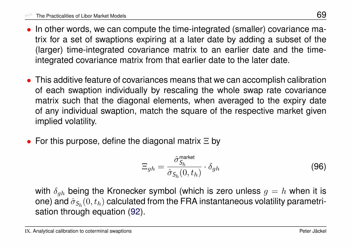
• In other words, we can compute the time-integrated (smaller) covariance ma-trix for a set of swaptions expiring at a later date by adding a subset of the(larger) time-integrated covariance matrix to an earlier date and the time-integrated covariance matrix from that earlier date to the later date.
• This additive feature of covariances means that we can accomplish calibrationof each swaption individually by rescaling the whole swap rate covariancematrix such that the diagonal elements, when averaged to the expiry dateof any individual swaption, match the square of the respective market givenimplied volatility.
• For this purpose, define the diagonal matrix Ξ by
Ξgh =σmarket
Sh
σSh(0, th)· δgh (96)
with δgh being the Kronecker symbol (which is zero unless g = h when it isone) and σSh(0, th) calculated from the FRA instantaneous volatility parametri-sation through equation (92).
IX. Analytical calibration to coterminal swaptions Peter Jäckel
The Practicalities of Libor Market Models 70
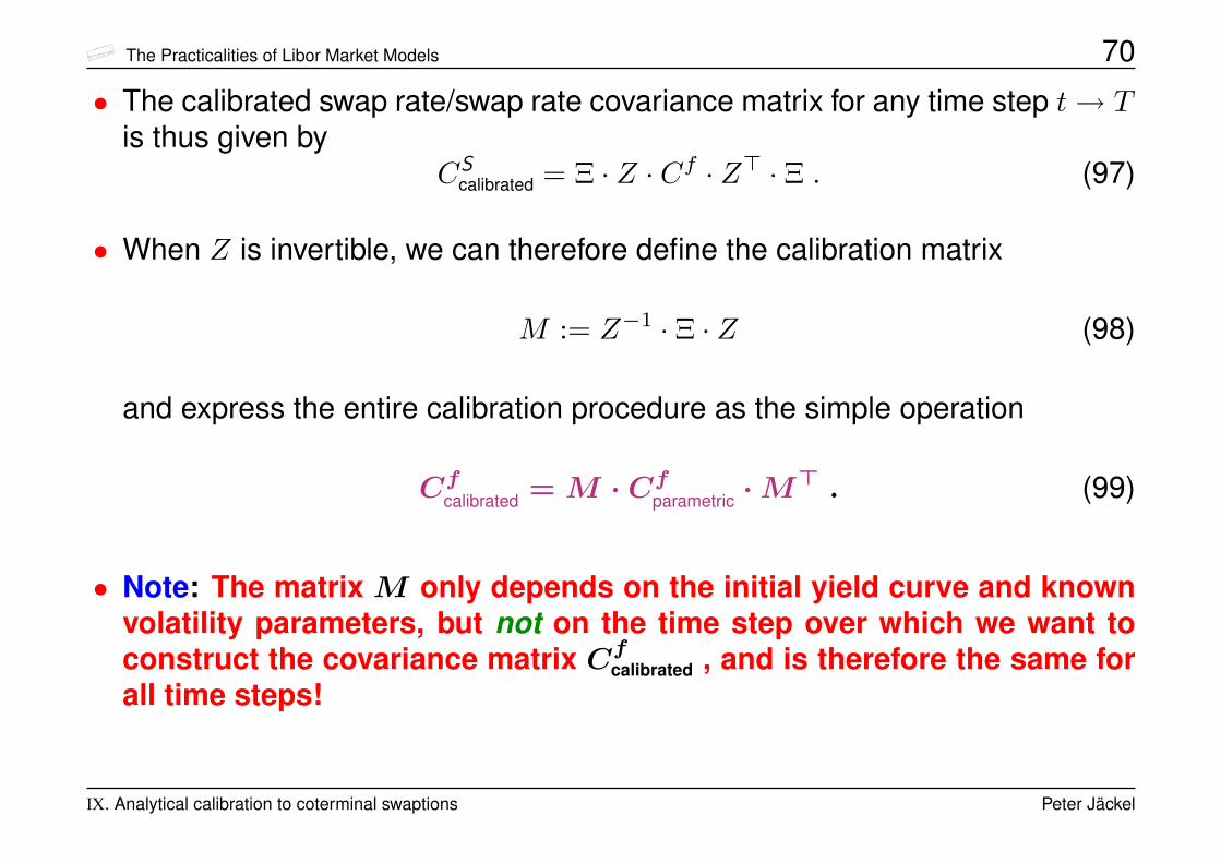
• The calibrated swap rate/swap rate covariance matrix for any time step t→ Tis thus given by
CScalibrated = Ξ · Z · Cf · Z> · Ξ . (97)
• When Z is invertible, we can therefore define the calibration matrix
M := Z−1 · Ξ · Z (98)
and express the entire calibration procedure as the simple operation
Cfcalibrated = M · Cfparametric ·M> . (99)
• Note: The matrix M only depends on the initial yield curve and knownvolatility parameters, but not on the time step over which we want toconstruct the covariance matrix Cfcalibrated , and is therefore the same forall time steps!
IX. Analytical calibration to coterminal swaptions Peter Jäckel
The Practicalities of Libor Market Models 71
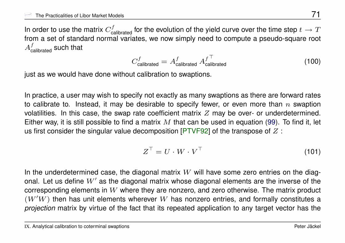
In order to use the matrix Cfcalibrated for the evolution of the yield curve over the time step t→ T
from a set of standard normal variates, we now simply need to compute a pseudo-square rootAf
calibrated such that
Cfcalibrated = A
fcalibrated A
fcalibrated>
(100)
just as we would have done without calibration to swaptions.
In practice, a user may wish to specify not exactly as many swaptions as there are forward ratesto calibrate to. Instead, it may be desirable to specify fewer, or even more than n swaptionvolatilities. In this case, the swap rate coefficient matrix Z may be over- or underdetermined.Either way, it is still possible to find a matrix M that can be used in equation (99). To find it, letus first consider the singular value decomposition [PTVF92] of the transpose of Z :
Z>
= U ·W · V > (101)
In the underdetermined case, the diagonal matrix W will have some zero entries on the diag-onal. Let us define W ′ as the diagonal matrix whose diagonal elements are the inverse of thecorresponding elements in W where they are nonzero, and zero otherwise. The matrix product(W ′W ) then has unit elements wherever W has nonzero entries, and formally constitutes aprojection matrix by virtue of the fact that its repeated application to any target vector has the
IX. Analytical calibration to coterminal swaptions Peter Jäckel

The Practicalities of Libor Market Models 72same result as a single multiplication, i.e.
(W′W )
k ·X = (W′W ) ·X ∀ k ≥ 1 and ∀X . (102)
The calibration procedure in the present framework amounts to the identification ofAfcalibrated that
satisfiesZ · Af
calibrated = Ξ · Z · Afparametric (103)
but remains as close to the original Afparametric as possible, i.e. to find the matrix Af
calibrated thatmeets equation (103) and simultaneously minimises˛˛
Afcalibrated − A
fparametric
˛˛(104)
for some suitable matrix norm. Denote the Moore-Penrose inverse [Alb72] of Z as Zf−1, andwrite the product of Zf−1 times Z itself as Q :
Q := U>−1
W′V> · VWU
> (105)
IX. Analytical calibration to coterminal swaptions Peter Jäckel

The Practicalities of Libor Market Models 73By the aid of the orthogonality conditions satisfied by the constituents U and V of the singularvalue decomposition of Z, and by the fact that (W ′W ) is a projection6, both Q and the matrix
P := 1−Q (106)
are also projection operators. In fact, P is the projection onto the kernel of Z. The desiredmatrix Af
calibrated can thus be found by adding the projection of Afparametric onto the kernel of Z
and the Moore-Penrose solution to equation (103), i.e.
Afcalibrated = P · Af
parametric + Zf−1 · Ξ · Z · Af
parametric . (107)
Since Afparametric appears as the last multiplicand in both of the summands on right hand side,
we can rewrite this as
Af
calibrated = (1− UW ′WU
>+ UW
′V>
ΞZ) · Afparametric
=“1− UW ′
“WU
> − V>ΞZ””· Afparametric
=“1− UW ′
“1− V >ΞV
”WU
>”· Afparametric . (108)
6 A projection operator is any operator T for which Tn = T for all n ≥ 1.
IX. Analytical calibration to coterminal swaptions Peter Jäckel
The Practicalities of Libor Market Models 74This means, the sought calibration matrix M is given by
M = 1− U ·W ′ ·“
1− V > · Ξ · V”·W · U> . (109)
The key to this calibration procedure in the underdetermined case is that a minimal solution tothe raw calibration problem (103) is combined with as much of the original covariance informationas possible that has no effect on the calibration problem. In more formal terms, we combine theminimal solution to the calibration problem with the projection of the desired covariance structureonto the calibration kernel.
When Z is overdetermined, the correction matrixM cannot achieve calibration to all the desiredmarket prices. Instead, the calibration procedure based on the linear algebraic operations abovewill result in a least squares fit in some suitable norm by virtue of the use of the singular valuedecomposition of Z.
Within the limits of the approximation (92), the operation given in equation (99) will providecalibration to European swaption prices whilst retaining as much calibration to the caplets as ispossible without violating the overall FRA/FRA correlation structure too much.
IX. Analytical calibration to coterminal swaptions Peter Jäckel

The Practicalities of Libor Market Models 75
X. Non-parametric volatility specification
Assume that we have a set of n forward rate fixing times (starting at the endof the accrual period of the spot Libor rate), and that the n associated forwardrates span the forward yield curve unambiguously.
Also, assume that we are satisfied with a discretisation of the term structure ofinstantaneous covariance at the same level of temporal resolution as the forwardrates themselves.
This means we can choose all correlation coefficients between all forward ratesover all time steps as well as all volatility coefficients for all forward rates over alltime steps at liberty to match any given set of calibration instruments.
X. Non-parametric volatility specification Peter Jäckel

The Practicalities of Libor Market Models 76
Note:
• The interest rates markets provide sufficient liquidity for the hedging of thelevel of volatility
Ü Hedging volatility is possible, and thus a market model should becalibrated to implied volatilities of relevant available contracts in themarket.
• The interest rates markets provide practically no direct hedge against thelevel of forward rate correlations.
Ü Efficiently hedging correlation is practically impossible, and thus amarket model should not try to calibrate correlation figures in a closedcalibration routine that disconnects the trader from any control overwhether the resulting correlation levels are realistic.
Numerical calibration of correlation coefficients is dangerous.
X. Non-parametric volatility specification Peter Jäckel

The Practicalities of Libor Market Models 77
Instead of a numerical calibration of a constant correlation structure, a reason-able parametrisation of the term structure of instantaneous correlation may bepreferred. This way, we can allow for the correlation of two adjacent forwardrates to gradually decrease as calendar time moves into the future.
In the following, we allow for stochastic stub evolution. However, since cali-bration instruments are not affected by this extension, it is not reasonable tocalibrate the stochastic stub volatility. In practice, it suffices to set it to the lastvolatility the corresponding just-fixed canonical rate experienced immediatelyprior to its fixing time.
This means, the number of free volatility coefficients σij we are at liberty tochoose for the discrete evolution set
ti → ti+1 for i = 1..n
is given byn∑i=1
n∑j=i
1 =12n(n+ 1) . (110)
X. Non-parametric volatility specification Peter Jäckel
The Practicalities of Libor Market Models 78
However, the number of correlation coefficients ρijk, which we choose in a rea-sonable fashion and not make the subject of any calibration procedure is
n∑i=1
n∑j=i
n∑k=j
1 =16n(n+ 1)(n+ 2) . (111)
In practice, we will never have 12n(n+1) calibration instruments of different expiry
and/or tenor.
It is thus prudent to choose a skeleton or reference volatility structureσreference(t, T ) = σreference(T − t) that is time-homogeneous and aim for calibrationthat is close to the reference structure.
X. Non-parametric volatility specification Peter Jäckel
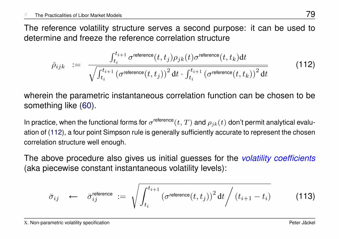
The Practicalities of Libor Market Models 79
The reference volatility structure serves a second purpose: it can be used todetermine and freeze the reference correlation structure
ρijk :=
∫ ti+1
tiσreference(t, tj)ρjk(t)σreference(t, tk)dt√∫ ti+1
ti(σreference(t, tj))
2 dt ·∫ ti+1
ti(σreference(t, tk))
2 dt(112)
wherein the parametric instantaneous correlation function can be chosen to besomething like (60).
In practice, when the functional forms for σreference(t, T ) and ρjk(t) don’t permit analytical evalu-ation of (112), a four point Simpson rule is generally sufficiently accurate to represent the chosencorrelation structure well enough.
The above procedure also gives us initial guesses for the volatility coefficients(aka piecewise constant instantaneous volatility levels):
σij ← σreferenceij :=
√∫ ti+1
ti
(σreference(t, tj))2 dt/
(ti+1 − ti) (113)
X. Non-parametric volatility specification Peter Jäckel

The Practicalities of Libor Market Models 80
XI. Global calibration to the full swaption matrix
For all caplets and swaptions7, an efficient and accurate approximate pricingformula of the form (92) can be found that links the Libor market model’s covari-ance structure directly to the corresponding implied volatility of the respectivecalibration instrument.
Thus, calibration to a specific swaption #l expiring at time tSl is given if theprimary calibration objective to reprice the market
(σatm
Sl
)2 =
i[tSl]∑
i=1
∑j,k
Zlj · σij · ρijk · σik · Zlk · (ti+1 − ti)
/tSl (114)
is satisfied withZlj =
∂Sl∂fj
fjSl
∣∣∣∣t=0
. (115)
7We shall treat caplets as a special case of swaptions from here on.
XI. Global calibration to the full swaption matrix Peter Jäckel
The Practicalities of Libor Market Models 81
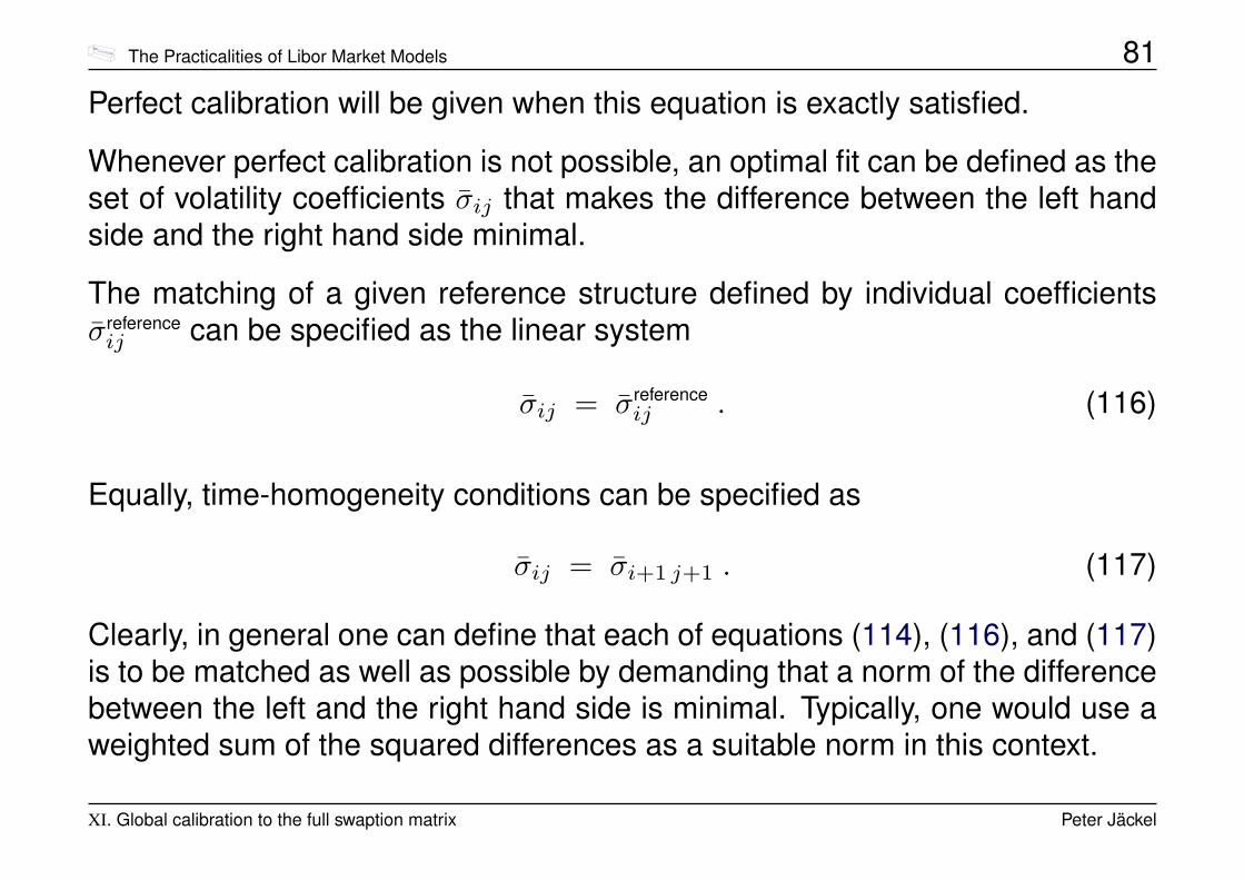
Perfect calibration will be given when this equation is exactly satisfied.
Whenever perfect calibration is not possible, an optimal fit can be defined as theset of volatility coefficients σij that makes the difference between the left handside and the right hand side minimal.
The matching of a given reference structure defined by individual coefficientsσreferenceij can be specified as the linear system
σij = σreferenceij . (116)
Equally, time-homogeneity conditions can be specified as
σij = σi+1 j+1 . (117)
Clearly, in general one can define that each of equations (114), (116), and (117)is to be matched as well as possible by demanding that a norm of the differencebetween the left and the right hand side is minimal. Typically, one would use aweighted sum of the squared differences as a suitable norm in this context.
XI. Global calibration to the full swaption matrix Peter Jäckel
The Practicalities of Libor Market Models 82
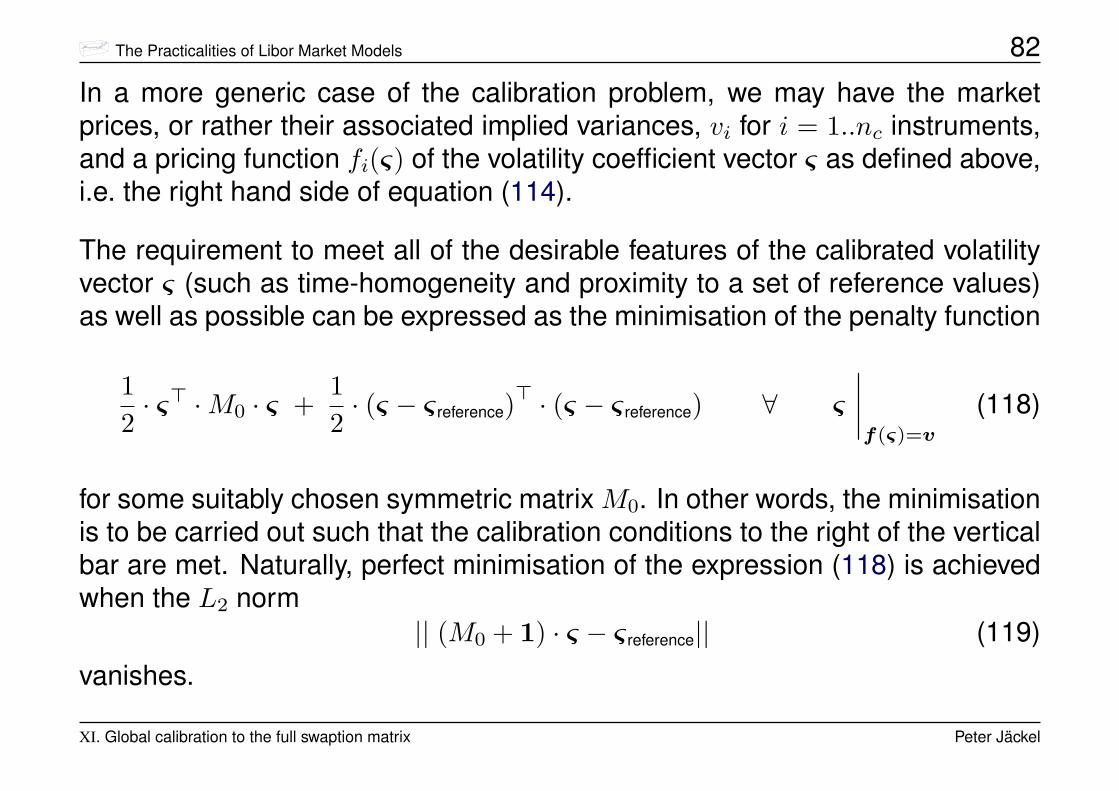
In a more generic case of the calibration problem, we may have the marketprices, or rather their associated implied variances, vi for i = 1..nc instruments,and a pricing function fi(ς) of the volatility coefficient vector ς as defined above,i.e. the right hand side of equation (114).
The requirement to meet all of the desirable features of the calibrated volatilityvector ς (such as time-homogeneity and proximity to a set of reference values)as well as possible can be expressed as the minimisation of the penalty function
12· ς> ·M0 · ς +
12· (ς − ς reference)
> · (ς − ς reference) ∀ ς
∣∣∣∣f(ς)=v
(118)
for some suitably chosen symmetric matrix M0. In other words, the minimisationis to be carried out such that the calibration conditions to the right of the verticalbar are met. Naturally, perfect minimisation of the expression (118) is achievedwhen the L2 norm
|| (M0 + 1) · ς − ς reference|| (119)
vanishes.
XI. Global calibration to the full swaption matrix Peter Jäckel
The Practicalities of Libor Market Models 83
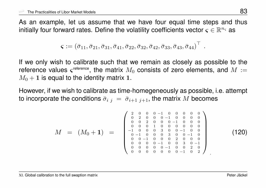
As an example, let us assume that we have four equal time steps and thusinitially four forward rates. Define the volatility coefficients vector ς ∈ Rnς as
ς := (σ11, σ21, σ31, σ41, σ22, σ32, σ42, σ33, σ43, σ44)> .
If we only wish to calibrate such that we remain as closely as possible to thereference values ς reference, the matrix M0 consists of zero elements, and M :=M0 + 1 is equal to the identity matrix 1.
However, if we wish to calibrate as time-homegeneously as possible, i.e. attemptto incorporate the conditions σi j = σi+1 j+1, the matrix M becomes
M = (M0 + 1) =
2 0 0 0 −1 0 0 0 0 00 2 0 0 0 −1 0 0 0 00 0 2 0 0 0 −1 0 0 00 0 0 1 0 0 0 0 0 0−1 0 0 0 3 0 0 −1 0 0
0 −1 0 0 0 3 0 0 −1 00 0 −1 0 0 0 2 0 0 00 0 0 0 −1 0 0 3 0 −10 0 0 0 0 −1 0 0 2 00 0 0 0 0 0 0 −1 0 2
.
(120)
XI. Global calibration to the full swaption matrix Peter Jäckel
The Practicalities of Libor Market Models 84
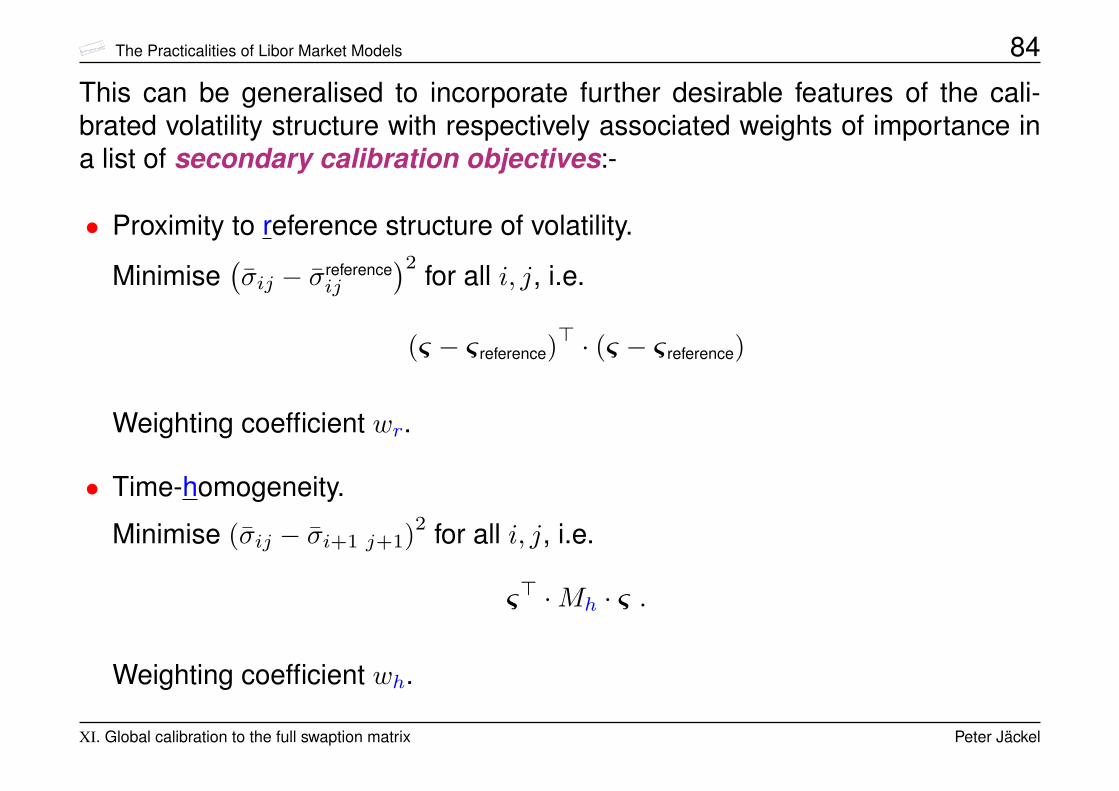
This can be generalised to incorporate further desirable features of the cali-brated volatility structure with respectively associated weights of importance ina list of secondary calibration objectives:-
• Proximity to reference structure of volatility.
Minimise(σij − σreference
ij
)2 for all i, j, i.e.
(ς − ς reference)> · (ς − ς reference)
Weighting coefficient wr.
• Time-homogeneity.
Minimise (σij − σi+1 j+1)2 for all i, j, i.e.
ς> ·Mh · ς .
Weighting coefficient wh.
XI. Global calibration to the full swaption matrix Peter Jäckel
The Practicalities of Libor Market Models 85
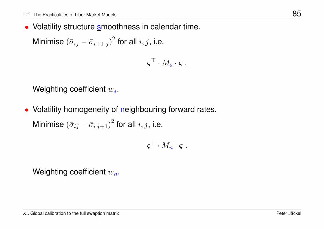
• Volatility structure smoothness in calendar time.
Minimise (σij − σi+1 j)2 for all i, j, i.e.
ς> ·Ms · ς .
Weighting coefficient ws.
• Volatility homogeneity of neighbouring forward rates.
Minimise (σij − σi j+1)2 for all i, j, i.e.
ς> ·Mn · ς .
Weighting coefficient wn.
XI. Global calibration to the full swaption matrix Peter Jäckel

The Practicalities of Libor Market Models 86
The calibration condition f(ς) = v is nonlinear and thus difficult to preserve inany minimisation of (118).
However, since our primary calibration criterion is the matching of the marketgiven variances, we ought to design a procedure whose main focus is on conver-gence to those, and only if there are any residual degrees of freedom in that pro-cedure should we exploit them for the sake of the given reference, homogeneity,and smoothness preferences such as the minimisation of expression (118).
We therefore start the development of our global calibration algorithm from thelocal linearisation of the calibration conditions as the governing equation ofan iterative procedure that leads from the current estimate ςk to the next es-timate ςk+1:
f(ςk) + J(ςk) · (ςk+1 − ςk)− v = 0 . (121)
Hereby, J(ς) ∈ Rnc×nς is the Jacobi matrix of the primary calibration criterion
J(ς) =∂ (f(ς))∂ (ς)
. (122)
XI. Global calibration to the full swaption matrix Peter Jäckel

The Practicalities of Libor Market Models 87
Due to the specific nature of our calibration problem, the function f(ς) happensto be symmetrically bilinear in the elements of ς. As a consequence, we have
f(ς) =12J(ς) · ς , (123)
and we can make use of this fact for optimisation.
From a geometric point of view, equation (121) means that the projection of theupdate vector
∆ςk := ςk+1 − ςk (124)onto each of the row vectors of J(ςk) must match the associated entry in thedifference vector
εk := v − f(ςk) , (125)i.e. the product of the increment vector ∆ςk with the Jacobi matrix Jk must equalthe difference vector εk:
Jk ·∆ςk − εk = 0 (126)
XI. Global calibration to the full swaption matrix Peter Jäckel
The Practicalities of Libor Market Models 88
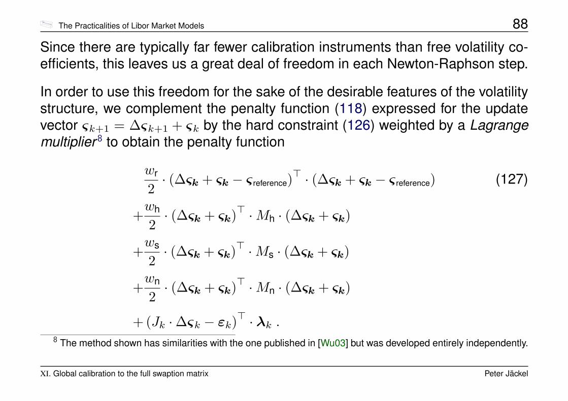
Since there are typically far fewer calibration instruments than free volatility co-efficients, this leaves us a great deal of freedom in each Newton-Raphson step.
In order to use this freedom for the sake of the desirable features of the volatilitystructure, we complement the penalty function (118) expressed for the updatevector ςk+1 = ∆ςk+1 + ςk by the hard constraint (126) weighted by a Lagrangemultiplier 8 to obtain the penalty function
wr
2· (∆ςk + ςk − ς reference)
> · (∆ςk + ςk − ς reference) (127)
+wh
2· (∆ςk + ςk)> ·Mh · (∆ςk + ςk)
+ws
2· (∆ςk + ςk)> ·Ms · (∆ςk + ςk)
+wn
2· (∆ςk + ςk)> ·Mn · (∆ςk + ςk)
+ (Jk ·∆ςk − εk)> · λk .8 The method shown has similarities with the one published in [Wu03] but was developed entirely independently.
XI. Global calibration to the full swaption matrix Peter Jäckel

The Practicalities of Libor Market Models 89
Note: the above penalty function is specific to the k-th step of the iterativeNewton-Raphson algorithm that we use to satisfy the primary calibration cri-terion.
Expression (127) is minimal with respect to all possible values of the vector ∆ςkwhen
M ·∆ςk + M · ςk − wr · ς reference − J>k · λk = 0 , (128)where we have used
M := wr1 + whMh + wsMs + wnMn . (129)
For wr 6= 0, the symmetic matrix M is positive definite and thus equation (128)can formally be solved for ∆ςk:
∆ςk = M−1 · J>k · λk − ςk + wr ·M−1 · ς reference (130)
XI. Global calibration to the full swaption matrix Peter Jäckel

The Practicalities of Libor Market Models 90
Since the last term on the right hand side remains constant throught the wholeNewton-Raphson process, we define
r := wrM−1ς reference (131)
and precompute it. Also, let us define the matrix H>k wit Hk ∈ Rnc×nς as thesolution of the linear system
M ·H>k = J>k . (132)
In this notation, we now have
∆ςk = H>k · λk − ςk + r (133)
Substituting this into the constraint that the increment ∆ςk must satisfy theNewton-Raphson condition (126), we obtain
Jk ·H>k · λk − Jk · ςk + Jk · r − εk = 0 . (134)
XI. Global calibration to the full swaption matrix Peter Jäckel

The Practicalities of Libor Market Models 91
Using the definitions
Gk = Jk ·H>k (135)
yk = εk + Jk · (ςk − r) (136)
we therefore obtain the vector of Lagrange multipliers λk as the solution of thelinear system from the symmetric matrix Gk ∈ Rnc×nc
Gk · λk = yk . (137)
Once we have computed λk ∈ Rnc, the updated vector ςk+1 is given by
ςk+1 = ςk + ∆ςk = H>k · λk + r . (138)
The key for fast calibration is the efficient solution of the involved large linear sys-tems. A very useful tool for this purpose is the Iterative Template Library [LLS].
XI. Global calibration to the full swaption matrix Peter Jäckel
The Practicalities of Libor Market Models 92
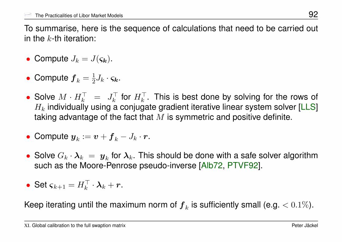
To summarise, here is the sequence of calculations that need to be carried outin the k-th iteration:
• Compute Jk = J(ςk).
• Compute fk = 12Jk · ςk.
• Solve M · H>k = J>k for H>k . This is best done by solving for the rows ofHk individually using a conjugate gradient iterative linear system solver [LLS]taking advantage of the fact that M is symmetric and positive definite.
• Compute yk := v + fk − Jk · r.
• Solve Gk · λk = yk for λk. This should be done with a safe solver algorithmsuch as the Moore-Penrose pseudo-inverse [Alb72, PTVF92].
• Set ςk+1 = H>k · λk + r.
Keep iterating until the maximum norm of fk is sufficiently small (e.g. < 0.1%).
XI. Global calibration to the full swaption matrix Peter Jäckel
The Practicalities of Libor Market Models 93
Mar-05
Mar-07
Mar-09
Mar-11
Mar-13
Mar-15
Mar-17
Mar-19
Mar-21
Mar-23
Mar-25
15-Mar-05
16-Mar-06
16-Sep-07
16-Mar-09
16-Sep-10
16-Mar-12
16-Sep-13
16-Mar-15
16-Sep-16
16-Mar-18
16-Sep-19
16-Mar-21
16-Sep-22
16-Mar-24
0%
10%
20%
30%
40%
50%
60%
70%
80%
Calendar time
Expiry
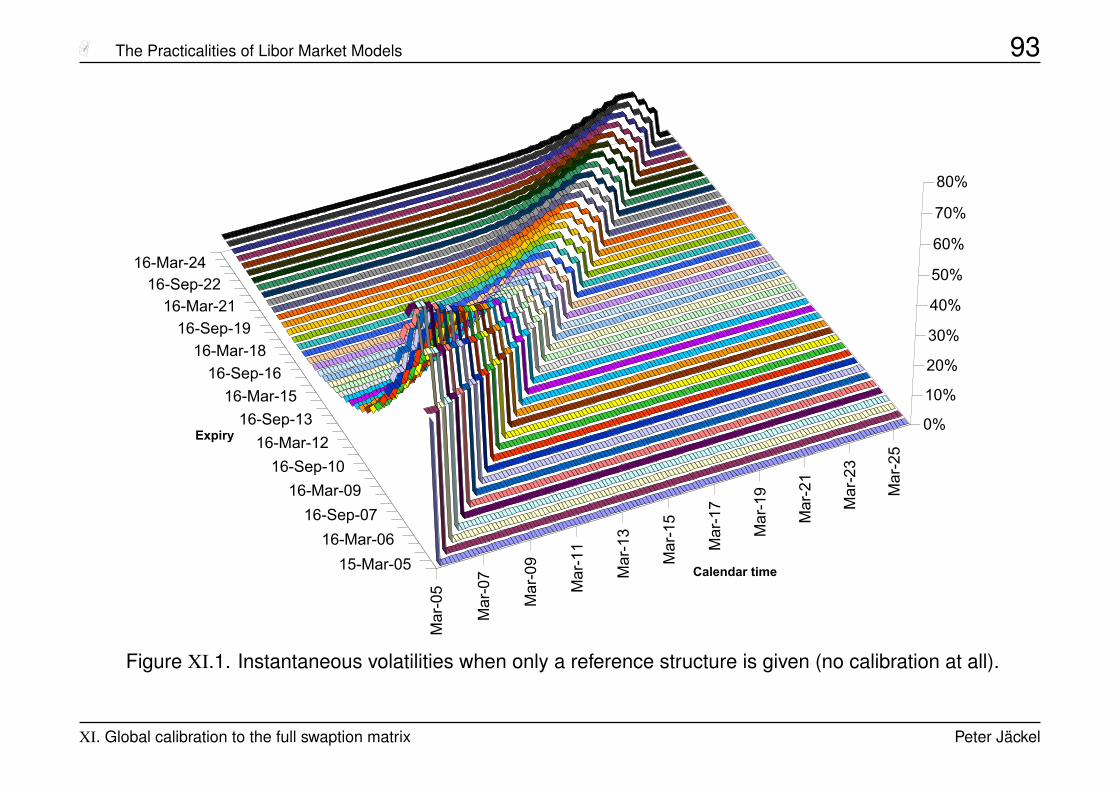
Figure XI.1. Instantaneous volatilities when only a reference structure is given (no calibration at all).
XI. Global calibration to the full swaption matrix Peter Jäckel
The Practicalities of Libor Market Models 94
Mar-05
Mar-07
Mar-09
Mar-11
Mar-13
Mar-15
Mar-17
Mar-19
Mar-21
Mar-23
Mar-25
15-Mar-05
16-Mar-06
16-Sep-07
16-Mar-09
16-Sep-10
16-Mar-12
16-Sep-13
16-Mar-15
16-Sep-16
16-Mar-18
16-Sep-19
16-Mar-21
16-Sep-22
16-Mar-24
0%
10%
20%
30%
40%
50%
60%
70%
80%
Calendar time
Expiry
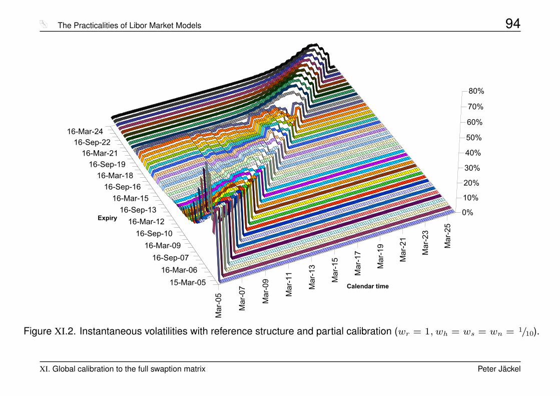
Figure XI.2. Instantaneous volatilities with reference structure and partial calibration (wr = 1, wh = ws = wn = 1/10).
XI. Global calibration to the full swaption matrix Peter Jäckel
The Practicalities of Libor Market Models 95
Mar-05
Mar-07
Mar-09
Mar-11
Mar-13
Mar-15
Mar-17
Mar-19
Mar-21
Mar-23
Mar-25
15-Mar-05
16-Mar-06
16-Sep-07
16-Mar-09
16-Sep-10
16-Mar-12
16-Sep-13
16-Mar-15
16-Sep-16
16-Mar-18
16-Sep-19
16-Mar-21
16-Sep-22
16-Mar-24
0%
10%
20%
30%
40%
50%
60%
70%
80%
Calendar time
Expiry
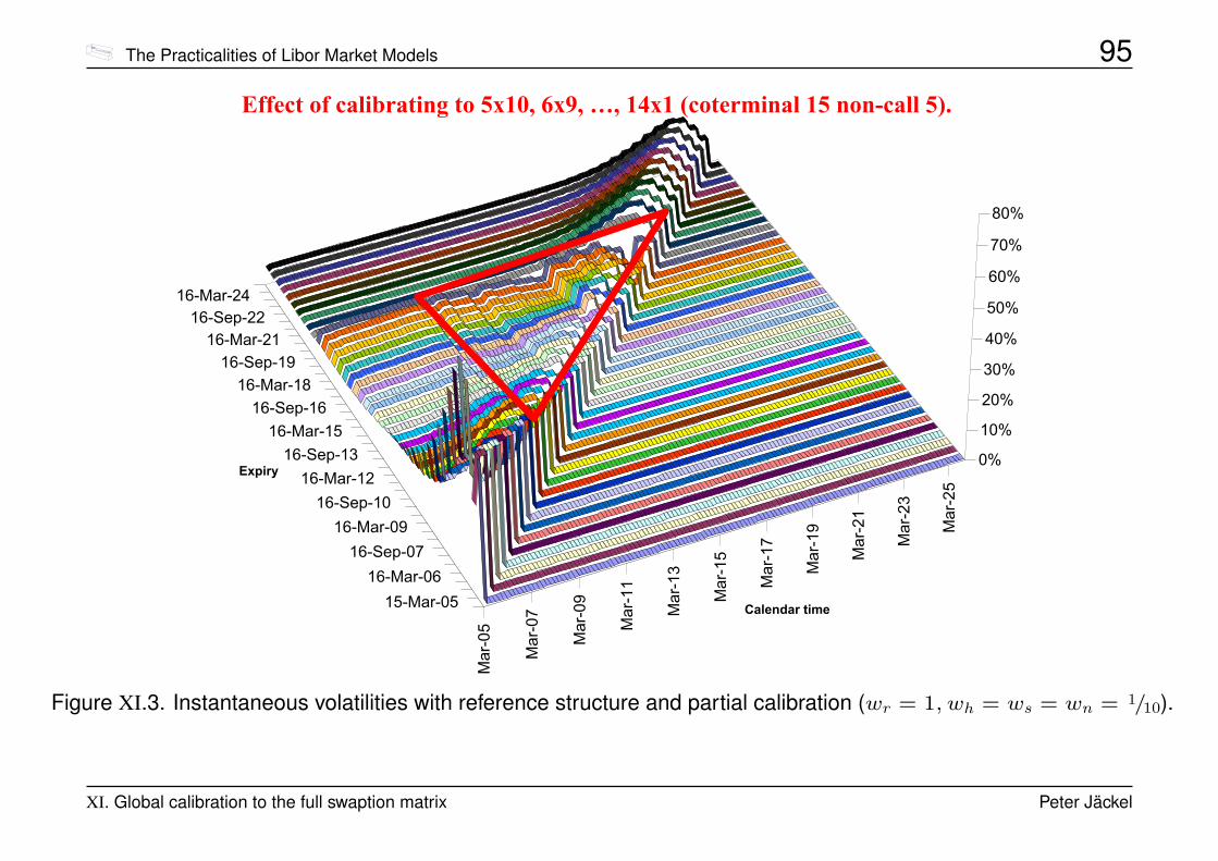
Effect of calibrating to 5x10, 6x9, …, 14x1 (coterminal 15 non-call 5).
Figure XI.3. Instantaneous volatilities with reference structure and partial calibration (wr = 1, wh = ws = wn = 1/10).
XI. Global calibration to the full swaption matrix Peter Jäckel

The Practicalities of Libor Market Models 96
Mar-05
Mar-07
Mar-09
Mar-11
Mar-13
Mar-15
Mar-17
Mar-19
Mar-21
Mar-23
Mar-25
15-Mar-05
16-Mar-06
16-Sep-07
16-Mar-09
16-Sep-10
16-Mar-12
16-Sep-13
16-Mar-15
16-Sep-16
16-Mar-18
16-Sep-19
16-Mar-21
16-Sep-22
16-Mar-24
0%
5%
10%
15%
20%
25%
30%
35%
40%
Calendar time
Expiry
Effect of global calibration
Figure XI.4. Instantaneous volatilities with reference structure and global calibration (wr = 1, wh = ws = wn = 10).
XI. Global calibration to the full swaption matrix Peter Jäckel
The Practicalities of Libor Market Models 97
XII. Bermudan Monte Carlo
For interest rate derivatives, the most common types of early exercise dealsnominally contain the prerogative of early termination.
When the concept of a prerogative of early termination is combined with an associated penaltypayment that may be contingent on market observables and be payable in either direction of thecontract, any early exercise specification can be accomodated.
Examples:
• Cancellable swap: swap + Bermudan swaption
• Option on option on option: three period cancellable irregular swap with be-spoke cashflow schedule
• Bermudan best-of call (max(S1, S2)−K)+: cancellable European option pay-ing (max(S1, S2)−K)+ at maturity with contingent penalty payment equal to(max(S1, S2)−K)+ payable to the prerogative holder.
XII. Bermudan Monte Carlo Peter Jäckel

The Practicalities of Libor Market Models 98
Contingent claims that allow exercise at a given set of discrete points in timeduring the life of the contract are frequently referred to as Bermudan9
For a specific Bermudan contract, the expected profit or loss to the option holderdepends on the strategy chosen by the holder of the prerogative.
A risk-neutral and perfectly rational investor will aim to find the strategy thatmaximises his profit.
For a set of discrete exercise opportunities tj for j = 1..m, a rational investor canconsider his exercise strategy as a set of m exercise decision indicator functionsthat all depend on the set of the prevailing financial state variables x(t) in therespective associated filtration.
Define the exercise decision function Ej(x(tj)) such that the right to terminate acontract at time tj is exercised if
Ej(x(tj)) > 0 .9 There are various different approaches for the valuation of such derivatives [And00, LS98, BG97a, BD96,
BG97b]. I present here my own tried-and-tested pet method.
XII. Bermudan Monte Carlo Peter Jäckel

The Practicalities of Libor Market Models 99
This means that today’s value of the contract for the given exercise strategyfunction vector E is given by
V0(x(0)) = E[1{E1(x(t1))>0} ·H1(x(t1)) + 1{E1(x(t1))≤0} · V1(x(t1))
]. (139)
H1: numéraire-denominated net present value of all the cashflows occurring ifthe given right is exercised at the first exercise opportunity t1.
V1: the value of the derivative contract if the prerogative is not exercised at t1.
The execise strategy dependent value of the contract is given by the recursivedefinition
Vj−1(x(tj−1)) = E[1{Ej(x(tj))>0} ·Hj(x(tj)) + 1{Ej(x(tj))≤0} · Vj(x(tj))
](140)
by setting t0 = 0.
In order to find the fair value of the given contingent claim in a risk-neutral mea-sure, let us view Vj as the objective function of an optimisation problem that isto find the exercise decision functions Ej+1, Ej+2, .., Em that maximise Vj.
XII. Bermudan Monte Carlo Peter Jäckel

The Practicalities of Libor Market Models 100
Fortunately, by virtue of the structure of equation (140) and by the aid of thetower law10, the recursive nature of the optimisation of the objective functiondecomposes into a sequence of non-recursive optimisations.
This can be seen by the fact that the optimisation of Ej does not depend at all on knowledge as to whether one
should ever exercise prior to tj at all: the optimisation of Ej only depends on the imminent and later exercise deci-
sion functions, not on earlier ones. This means that the last exercise decision function Em can be optimised entirely
without the influence of any other strategic considerations other than the one at tm. Once we have knowledge of the
optimal function Em, however, the optimisation of Em−1, in turn, becomes a well defined optimisation problem in
which only Em−1 needs to be varied (since the truly optimal Em is already known) until Vm−1 is maximised. Thus,
the fair value of the derivative contract can be computed in a procedure in which a sequence of exercise strategy
functions are optimised in their reverse order in time. The reverse order highlights the connection to conventional
tree or finite differencing schemes: the fair value can only be computed with a method of backwards induction type.
It is, in general, not possible on a finite computer to implement an algorithm thatcan find the very optimal out of all possible exercise decision functions.
One can, however, devise methods that are able to come very close.10also known as the law of iterated conditional expectations
XII. Bermudan Monte Carlo Peter Jäckel

The Practicalities of Libor Market Models 101A very simple, yet equally very robust, approach to achieve this is to rely on a suitable parametri-sation of the sought exercise decision function and thus to change the nature of the optimisationproblem from the search for the optimal function (which is really a problem of functional analysisand thus much harder to implement numerically) to the search for the optimal parameters. Theimplementation of the prerogative-of-early-termination algorithm can thus make use of the greatnumerical simplification that is given by the provision of a suitable parametrisation of the exer-cise decision function. Also, it is in general the case that not all state variables are needed fora good approximation to the optimal exercise decision function. Indeed, in most applications (infact all I have seen so far), a projection of the state space variables onto a small set of financiallyrelevant coordinates, say the vector f j associated with time tj, suffices for a highly accurateoptimisation.
In the following, the exercise decision function associated with exercise at timetj is from here on denoted as
Ej(f j;λj)with λj being a vector of parameters solely responsible for exercise at time tj.Note that we make no assumption that the parametric form of the exercise decision function, the number of parameters, the choice offinancial coordinates, or the number of financial coordinates is the same for different exercise times. In practice though, due to mostcallable derivative structures having a large degree of time homogeneity in their contract definition, the functional and parametric form maybe the same for all exercise dates.
XII. Bermudan Monte Carlo Peter Jäckel

The Practicalities of Libor Market Models 102
The prerogative-of-early-termination algorithm leaves two very important tasksup to the designer of the functional and parametric form of the exercise decisionfunction: a good approximation to the fair value can only be achieved
1. with a suitable choice of financial coordinates and
2. a reasonably flexible parametric form that allows for a good fit to the trulyoptimal exercise frontier.
Both ot these choices depend typically very heavily on the contract structure,but, luckily, rarely on the actual model employed for the valuation. This meansone can use the same parametrisation with a Hull-White model, or a Libor mar-ket model, or indeed any other reasonably well calibrated model!
Also, in all cases (the author has) seen so far it is possible to find a suitableexercise decision functional form that is robust with respect to the magnitudeof the market parameters which is a crucial feature for the prerogative-of-early-termination algorithm to be a viable method in an integrated pricing system.
XII. Bermudan Monte Carlo Peter Jäckel
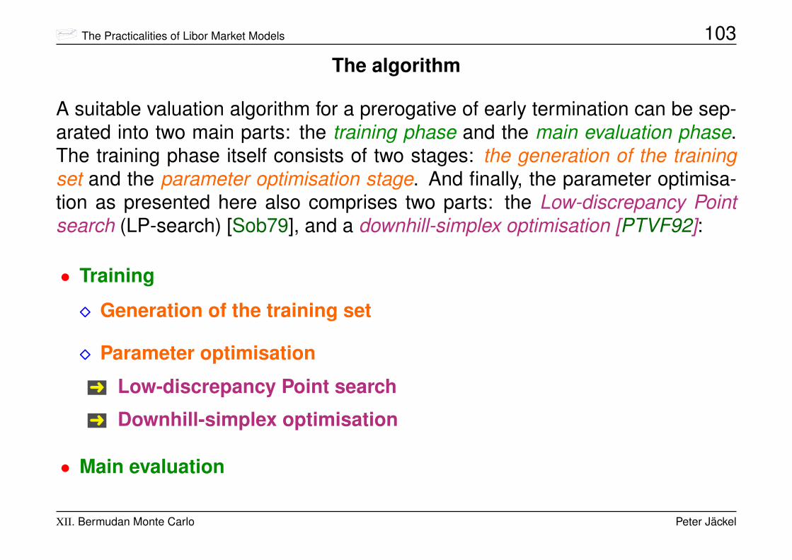
The Practicalities of Libor Market Models 103
The algorithm
A suitable valuation algorithm for a prerogative of early termination can be sep-arated into two main parts: the training phase and the main evaluation phase.The training phase itself consists of two stages: the generation of the trainingset and the parameter optimisation stage. And finally, the parameter optimisa-tion as presented here also comprises two parts: the Low-discrepancy Pointsearch (LP-search) [Sob79], and a downhill-simplex optimisation [PTVF92]:
• Training
� Generation of the training set
� Parameter optimisation
Ü Low-discrepancy Point search
Ü Downhill-simplex optimisation
• Main evaluation
XII. Bermudan Monte Carlo Peter Jäckel

The Practicalities of Libor Market Models 104
The training phase
The starting point of the prerogative-of-early-termination methodology is thegeneration of a training set.
In a simplified way, one can think of the training set as a presimulated set ofMonte Carlo evolution paths.
In practice, however, only the information relevant for the subsequent parameteroptimisation is generated along any one path.
Generation of the training set
Let the
• number of paths in the training set be denoted as n,
and the
• number of exercise time horizons as m.
XII. Bermudan Monte Carlo Peter Jäckel

The Practicalities of Libor Market Models 105
Then, for each path indexed by the integer i, start the evaluation of the sequenceof cashflow events (indexed by the integer j) at the beginning of the productdescription timeline, and aggregate the sum of cashflows divided by the valueof the numéraire asset out to each exercise time horizon:
aij :=j∑l=1
cilNil
. (141)
Hereby, cil stands for the value of the cashflow occuring in path #i at event #l,and Nil stands for the value of the numéraire asset in the same path at the samepoint in time.
When an exercise of the prerogative occurs on path #i at a given time hori-zon #j, the value of the path is the aggregated path value aij, amended by thepenalty payment pij that is to be made there and then in case of early termina-tion.
XII. Bermudan Monte Carlo Peter Jäckel

The Practicalities of Libor Market Models 106
We denote the value of the path #i conditional on cancellation occurring at timehorizon #j by
πij := aij +pijNij
. (142)
Naturally, it is possible for no termination to occur at all for any one given path#i.
Let the aggregate of all the cashflow payments divided by their associatednuméraire asset values be denoted as the complete path continuation valueqi.
In addition to the cancellation path values πij and the continuation path valuesqi, we also need to compute the financial coordinate values associated with eachpath at each exercise time horizon.
In the following, we denote the financial coordinate value in path #i at event #jfor the coordinate #s as fijs.
XII. Bermudan Monte Carlo Peter Jäckel
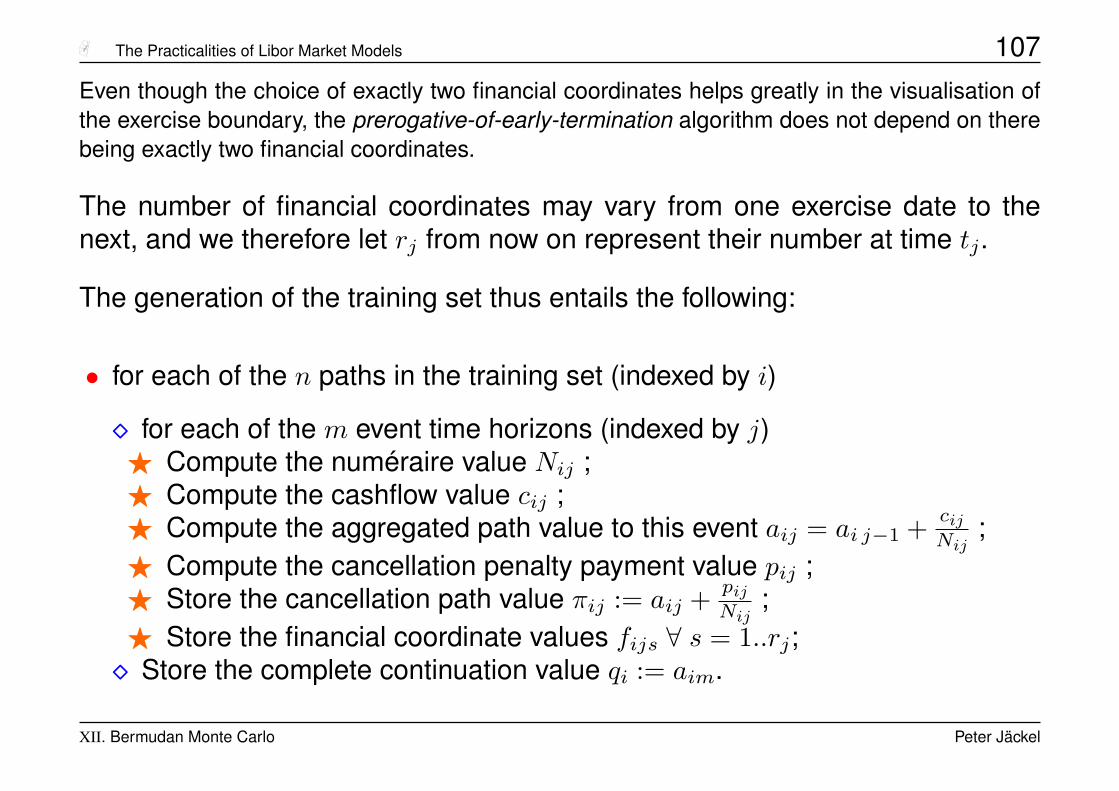
The Practicalities of Libor Market Models 107Even though the choice of exactly two financial coordinates helps greatly in the visualisation ofthe exercise boundary, the prerogative-of-early-termination algorithm does not depend on therebeing exactly two financial coordinates.
The number of financial coordinates may vary from one exercise date to thenext, and we therefore let rj from now on represent their number at time tj.
The generation of the training set thus entails the following:
• for each of the n paths in the training set (indexed by i)
� for each of the m event time horizons (indexed by j)F Compute the numéraire value Nij ;F Compute the cashflow value cij ;F Compute the aggregated path value to this event aij = ai j−1 + cij
Nij;
F Compute the cancellation penalty payment value pij ;F Store the cancellation path value πij := aij + pij
Nij;
F Store the financial coordinate values fijs ∀ s = 1..rj;� Store the complete continuation value qi := aim.
XII. Bermudan Monte Carlo Peter Jäckel

The Practicalities of Libor Market Models 108
The training set is therefore concisely described by a set of
n · (m · (r + 1) + 1)
numbers.
Since, for some models, the number of state space variables is much greaterthan the number of important financial coordinates for any one given producet,storing all of the underlying financial variables for each path and each eventhorizon can easily pose a prohibitively large memory requirement.
By only storing the preprocessed relevant information associated with each pathand each event horizon, the storage needs can be greatly reduced and thus isno issue for the implementation of the algorithm.
XII. Bermudan Monte Carlo Peter Jäckel

The Practicalities of Libor Market Models 109
The objective function
Given a specified exercise decision function Ej(f j;λj) associated with the pre-rogative at time tj, the aim of the training phase is thus to find the parametervalues λj = λ∗j such that the objective function
Vj :=1n
n∑i=1
[1{Ej(f ij;λj)>0} · πij + 1{Ej(f ij;λj)≤0} · qi
](143)
takes on its maximal value over all possible choices for λj.
This optimisation has to be carried out individually for each exercise time, andthe optimisations over all j have to be done in reverse order, i.e.
j = m, (m− 1), (m− 2), ..., 2, 1.
XII. Bermudan Monte Carlo Peter Jäckel

The Practicalities of Libor Market Models 110
The key to the efficiency of the algorithm is that, following each optimisation ofa specific parameter vector λj to find the optimal values λ∗j , the continuationvariable values qi for i = 1, .., n are updated given the then known values λ∗j .
In other words, after the optimisation procedure has converged to the values λ∗j ,we override the continuation variable values
qi := 1{Ej(f ij;λ∗j)>0} · πij + 1{Ej(f ij;λ∗j)≤0} · qi . (144)
In practice, this of course means that we update each continuation variable valueonly if the just optimised exercise decision function Ej indicates that for path #iexercise should occur at time tj.
The benefit of this scheme is that the optimisation of m exercise decision func-tions’ parameters is a task whose computation time grows only linearly in msince none of the later exercise decision functions are ever evaluated againonce they have been optimised.
XII. Bermudan Monte Carlo Peter Jäckel
The Practicalities of Libor Market Models 111
Strictly speaking, this procedure results in a value for V0 that is upwards biased due to the factthat the same set of paths is used for the optimisation of all exercise decision functions, thoughthe bias diminishes quickly with increasing number of paths in the training set.
Fortunately, this poses no major problem since we can obtain an unbiased estimate for thefair value of the derivative contract by invoking a second Monte Carlo simulation that uses theoptimised exercise decision functions but is based on a completely new set of simulated paths.
To avoid any upwards bias altogether, the prerogative-of-early-terminationmethod consists of two parts, and it is the second part, the main valuationphase, that comprises the required simulation using a new set of paths gen-erated to avoid an upwards bias in the final estimate for the derivative’s value.
Parameter optimisation on the training set
As an example, let us assume that the financial variables of relevance of thecancellable derivative contract at hand span a two-dimensional coordinate sys-tem. Let us also assume that the training set consists of 2047 paths resulting inthe same number of event coordinate pairs at each event date.
XII. Bermudan Monte Carlo Peter Jäckel
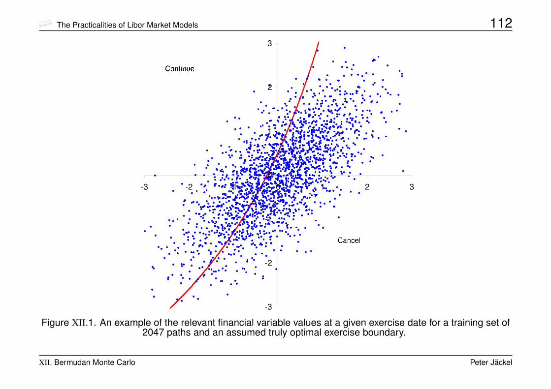
The Practicalities of Libor Market Models 112
Figure XII.1. An example of the relevant financial variable values at a given exercise date for a training set of2047 paths and an assumed truly optimal exercise boundary.
XII. Bermudan Monte Carlo Peter Jäckel
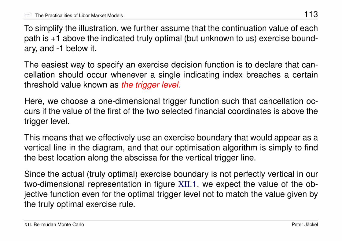
The Practicalities of Libor Market Models 113
To simplify the illustration, we further assume that the continuation value of eachpath is +1 above the indicated truly optimal (but unknown to us) exercise bound-ary, and -1 below it.
The easiest way to specify an exercise decision function is to declare that can-cellation should occur whenever a single indicating index breaches a certainthreshold value known as the trigger level.
Here, we choose a one-dimensional trigger function such that cancellation oc-curs if the value of the first of the two selected financial coordinates is above thetrigger level.
This means that we effectively use an exercise boundary that would appear as avertical line in the diagram, and that our optimisation algorithm is simply to findthe best location along the abscissa for the vertical trigger line.
Since the actual (truly optimal) exercise boundary is not perfectly vertical in ourtwo-dimensional representation in figure XII.1, we expect the value of the ob-jective function even for the optimal trigger level not to match the value given bythe truly optimal exercise rule.
XII. Bermudan Monte Carlo Peter Jäckel
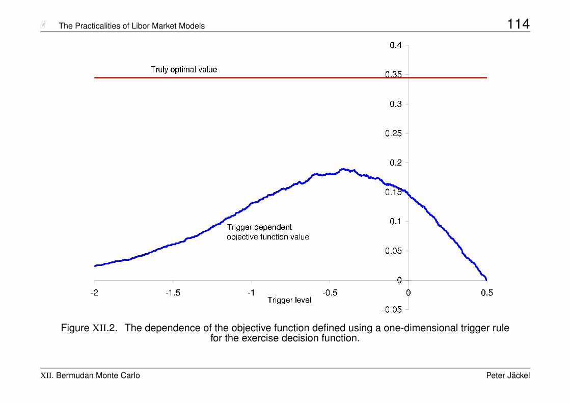
The Practicalities of Libor Market Models 114
Figure XII.2. The dependence of the objective function defined using a one-dimensional trigger rulefor the exercise decision function.
XII. Bermudan Monte Carlo Peter Jäckel
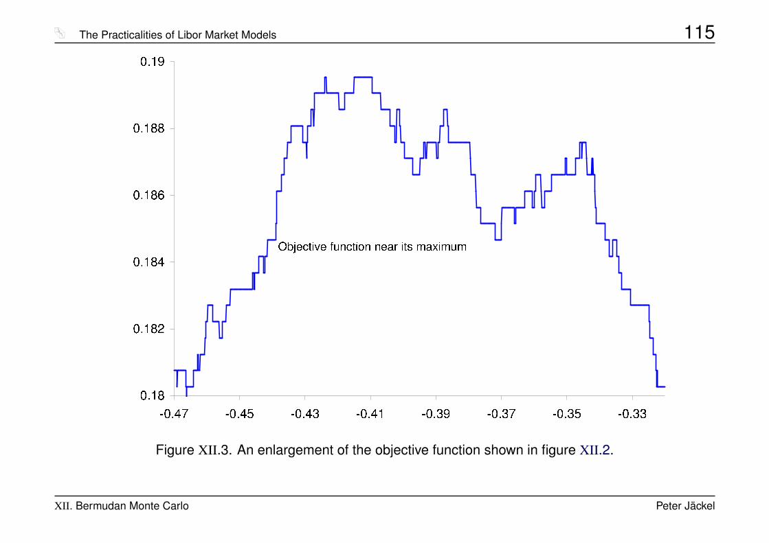
The Practicalities of Libor Market Models 115
Figure XII.3. An enlargement of the objective function shown in figure XII.2.
XII. Bermudan Monte Carlo Peter Jäckel

The Practicalities of Libor Market Models 116
There are two interesting features to note here:
1. The objective function appears to be piecewise constant.
2. The maximum of the function is not well defined.
Both observations can be readily explained:
Recall that the objective function is defined using a small set of discretelysampled training paths, and thus the distribution of the financial coordinatevalue pairs and the associated continuation values are subject to the usualerror we incur in any Monte Carlo simulation.
This explains why there is more than one local maximum near what wewould expect to be the location of the overall global maximum. In the limitof infinitely many paths in the training set, the function would converge tohaving a single local maximum. In other words, the fact that the maximumis not clearly defined is simply due to the inevitable presence of noise.
XII. Bermudan Monte Carlo Peter Jäckel

The Practicalities of Libor Market Models 117
The piecewise constant nature of the objective function is also not difficult tounderstand:
It is caused by the fact that the objective function can only ever changevalue as and when the trigger level slides over the coordinate value of oneof the event points in the training set.
Note: the locally noisy nature of the global maximum and the piecewise con-stant nature of the objective function are both genuinely intrinsic features of theprerogative-of-early-termination valuation methodology and not just artefacts ofour choice of a one-dimensional exercise decision function.
The above mentioned features of the objective function have an important con-sequence with respect to the choice of the optimisation algorithm: since theobjective function is piecewise constant, its local gradient is always zero andthus methods based on an analytically computed gradient are not applicable!
XII. Bermudan Monte Carlo Peter Jäckel
The Practicalities of Libor Market Models 118Of course, one can, instead of computing the gradient analytically, use a finite differencing algorithm for theapproximation of the slope.
However, the use of a finite differencing algorithm requires knowledge of a suitable length scale to be used forthe numerical differentiation.
Unfortunately, since the prerogative-of-early-termination method has to be robust with respect to changesof the product under consideration, market parameters, and other details, it would be very difficult indeed todesign a finite differencing algorithm for the numerical approximation of the local gradient of sufficient reliablility.
In addition to that, the fact that the global maximum is always subject to some local noise makes it practicallyimpossible to use one of the many optimisation methods based on the local gradient that can be found in theliterature.
To summarise:
• We cannot use a local gradient method easily.
• There may appear to be more than one local maximum.
• We cannot use a numerical approximation for the gradient based on any sin-gle estimate of the appropriate length scale.
XII. Bermudan Monte Carlo Peter Jäckel

The Practicalities of Libor Market Models 119
All is not lost, though!
We can use a method that changes its numerical length scale of spatialexploration in each and every iteration, first roaming the parameter spacerather coarsely and then refining its search in the most promising area forthe global maximum!
A very simple algorithm with this feature is known as the downhill-simplex algo-rithm [PTVF92].
A simplex in d dimensions is essentially the volume spanned by (d + 1) linearlyindependent corner points.
In two dimensions, a simplex is simply a triangle. In three dimensions, a simplexis a terahedron, and so forth.
To start the downhill-simplex algorithm, we need (d + 1) initial guesses for theparameter vector λ.
XII. Bermudan Monte Carlo Peter Jäckel

The Practicalities of Libor Market Models 120
Since it is in practice hard enough to demand the provision of one initial guess,we need a systematic method to generate those required (d+1) simplex startingpoints.
One way to overcome this problem is to use a so-called LP-search [Sob79].
In this context, an LP-search is nothing other than, given an initial guess, theattempt to find other suitable points by sampling in the vicinity of the initial guessusing a Sobol’ vector sequence and some suitably selected joint distribution ofall the parameter vector entries.
The implementation therefore requires the user to specify
• an initial guess for the exercise decision function parameter vector,
• a vector of standard deviations for each parameter,
• and the number of LP-search points that are to be used.
XII. Bermudan Monte Carlo Peter Jäckel

The Practicalities of Libor Market Models 121
In practice, 63 LP-search points are usually enough when the exercise decisionfunction has up to five parameters and a reasonable initial guess is provided.
The (d + 1) simplex corner points can simply be chosen to be the (d + 1) bestguesses resulting from the initial LP-search.
The subsequent downhill-simplex algorithm is then invoked and continued untileither the objective function converges on a relative scale (no further signifi-cant improvement of the function value possible) or until the simplex has beencontracted by the algorithm to a comparatively small size (no further significantprogress in parameter space).
The valuation phase
After the completion of the training phase, the prerogative-of-early-terminationmethod continues with the main valuation.
This consists of an essentially independent Monte Carlo simulation using newlygenerated paths for the financial state variables. All exercise decisions are nowtaken on the basis of the fixed (optimised) parameter values.
XII. Bermudan Monte Carlo Peter Jäckel
The Practicalities of Libor Market Models 122
Information loss due to inappropriate projection
The prerogative-of-early-termination method is very flexible to adapt to manydifferent possible products and thus exercise domain types.
For instance, it is possible to design a function that is positive in several dis-joint regions that are each individually well behaved singly connected exercisedomains.
An application for such an exercise decision function parametrisation would bea Bermudan style option on the maximum of two assets against a fixed strike,i.e. an option with intrinsic value (max(S1, S2)−K)+.
However, since the flexibility is to some extent achieved by leaving the designof the exercise decision function parametrisation up to the financial engineertayloring the product description, it is also possible to end up with noticeableundervaluation of the optionality in a given product due to an unfortunate mis-specification of the exercise decision function.
XII. Bermudan Monte Carlo Peter Jäckel
The Practicalities of Libor Market Models 123
This is in itself not surprising.
A particularly dramatic example of this is that it is possible for an unfortu-nate mis-specification of an exercise decision function parametrisation with theprerogative-of-early-termination optimisation method to result in an option valuethat is lower than the value that can be obtained from a heuristically guessedset of parameters used with the same exercise decision function.
This may look at first as if the optimisation algorithm failed in its task and can bevery confusing.
In order to explain how this phenomenon can arise, and to show that, when ithappens, it really is simply due to the fact that a very important financial dimen-sion has been ignored, we revisit the example in figure XII.1.
Recall that the maximum of the unconditional objective function as a function ofthe trigger level parameter in figure XII.3 was near the abscissa value -0.42.
XII. Bermudan Monte Carlo Peter Jäckel
The Practicalities of Libor Market Models 124
This would mean that the approximate exercise boundary given the simple one-dimensional trigger function approach would result in the effective exercise strat-egy boundary given by a vertical line at abscissa value -0.42 in figure XII.1.
Now, let us assume that instead of only one single exercise event, as we had sofar in the example in figure XII.1, there is now one further exercise event at aslightly earlier date.
We arbitrarily choose the earlier exercise event to cause early cancellation of allpaths whose second coordinate is above -0.5 at that earlier date.
Since we assume some kind of two-dimensional diffusion process behind thepath evolution, this means that out of all of our initially given 2047 sample paths,only a fraction ever arrives at the later event date we are interested in.
XII. Bermudan Monte Carlo Peter Jäckel

The Practicalities of Libor Market Models 125
Figure XII.4. The value of the conditional objective function can be significantly lower when the parameter optimisation is carried out onan unconditional training set (backwards induction) when important financial variables were ignored (here: the second coordinate axis).
Only paths that prevail to the later (this) event date are marked as scattered dots.
XII. Bermudan Monte Carlo Peter Jäckel
The Practicalities of Libor Market Models 126
Note that figure XII.4 is not exactly on the same scale as figure XII.1 which iswhy the scattered data set may appear somewhat distorted.
If you carefully compare the shape and location of several clusters you willrecognise that it is indeed part of the same data set.
You may also note that some paths arrive at this event above the ordinate value-0.5, which is naturally caused by the diffusion process between the first and thesecond date.
The abscissa value of the right hand side vertical line is at -0.42 and correspondsto the one-dimensional trigger level that was obtained from the optimisation overthe original, unconditional, training set.
The objective value associated with that trigger level for the unconditional train-ing set, i.e. averaging over all paths in the training set without any filtering at anearlier event date, was approximately 19%.
XII. Bermudan Monte Carlo Peter Jäckel
The Practicalities of Libor Market Models 127
However, if we restrict the averaging to those paths that actually arrive at thelater event date due to the fact that many are already cancelled at an earlierdate, we obtain a conditional objective function value of only around 6% whenthe one-dimensional trigger level is set at -0.42.
If, on the other hand, we now optimise the trigger level over the conditionaltraining set, i.e. only over those paths that actually make it to the second eventdate, we find that a conditional trigger level of around -0.9 gives us a conditionalobjective function value of 9%.
In comparison, the true conditional objective function value, i.e. the value weobtain when using the actually optimal exercise boundary given by the solid lineis 13%.
XII. Bermudan Monte Carlo Peter Jäckel
The Practicalities of Libor Market Models 128
Whilst this example is somewhat contrived, it highlights the following problem:since the parameter optimisation of the prerogative-of-early-termination functionis for efficiency reasons done in a backward induction fashion at each eventdate on the event set that takes no notice of earlier exercise opportunities, it ispossible for the optimisation procedure to produce suboptimal parameter valueswhen the exercise decision function disregards important financial coordinates.
It is important to emphasise, though, that this kind of problem is extremely rareand only occurs when either a single, comparatively simple, exercise decisionfunction is used for a set of exercise events with strongly varying exercise bound-ary features due to the nature of the contract changing its characteristics in amajor way throughout the life of the deal, or, when an extremely important finan-cial coordinate has been disregarded completely in the design of the exercisedecision function.
XII. Bermudan Monte Carlo Peter Jäckel
The Practicalities of Libor Market Models 129
An example where the above described phenomenon has been observed in practice wasa callable swap whose structured coupons are determined by an accreting ratchet formula,whereby the exercise decision function was indeed initially set to be a one-dimensional triggerrule.
Since the accreting factor is a strongly path-dependent variable for this kind of product, it provedto be essential that the exercise decision function took it into account.
Changing the exercise decision function to a two-dimensional rule with one of the financial co-ordinates being the accreting factor immediately remedied the issue.
An alternative solution to the phenomenon described in this section would be todesign a variation of the prerogative-of-early-termination optimisation procedurethat always optimises on the conditional training set.
Since this approach would result in a growth of the calculation time quite easilyfrom being linear in the number of event dates, to being quadratic in the numberof event dates, it is at present not envisaged to implement this alternative.
XII. Bermudan Monte Carlo Peter Jäckel

The Practicalities of Libor Market Models 130
Applied example: Bermudan swaption.
0%
5%
10%
15%
20%
25%
30%
0% 5% 10% 15% 20% 25% 30%
f� 1�
f0
intrinsic < discounted expectation
intrinsic > discounted expectation
Figure XII.5. Bermudan swaption exercise domain computed with a non-recombining tree in Libor/Libor projection.
XII. Bermudan Monte Carlo Peter Jäckel
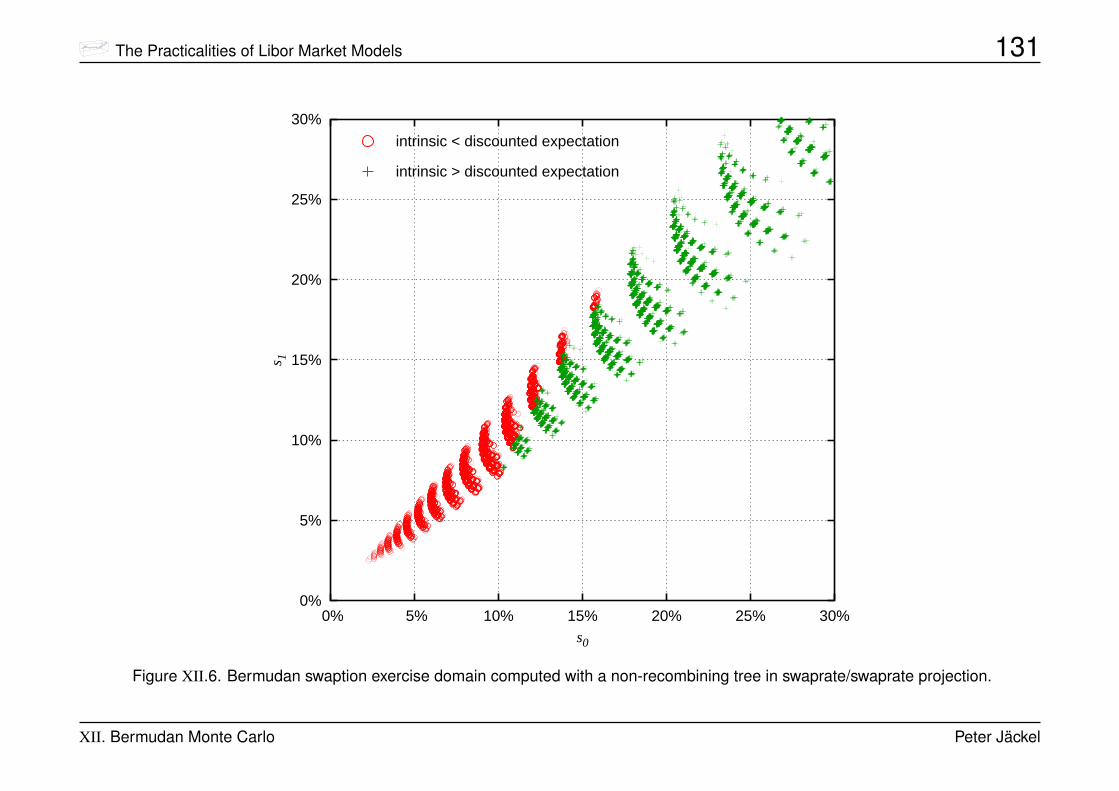
The Practicalities of Libor Market Models 131
0%
5%
10%
15%
20%
25%
30%
0% 5% 10% 15% 20% 25% 30%
s 1
s0
intrinsic < discounted expectation
intrinsic > discounted expectation
Figure XII.6. Bermudan swaption exercise domain computed with a non-recombining tree in swaprate/swaprate projection.
XII. Bermudan Monte Carlo Peter Jäckel

The Practicalities of Libor Market Models 132
0
0.2
0.4
0.6
0.8
1
1.2
1.4
0 0.5 1 1.5 2
s 1*B
1
s0*B0
intrinsic < discounted expectation
intrinsic > discounted expectation
Figure XII.7. Bermudan swaption exercise domain computed with a non-recombining tree in floating-leg/floating-leg projection.
XII. Bermudan Monte Carlo Peter Jäckel

The Practicalities of Libor Market Models 133
0%
5%
10%
15%
20%
25%
30%
0% 5% 10% 15% 20% 25% 30%
s 1
f0
intrinsic < discounted expectation
intrinsic > discounted expectation
Figure XII.8. Bermudan swaption exercise domain computed with a non-recombining tree in floating-leg/swaprate projection.
XII. Bermudan Monte Carlo Peter Jäckel
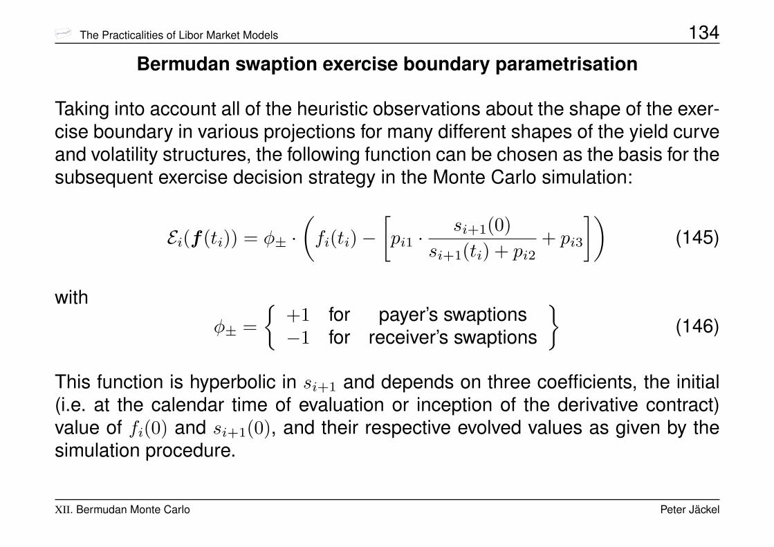
The Practicalities of Libor Market Models 134
Bermudan swaption exercise boundary parametrisation
Taking into account all of the heuristic observations about the shape of the exer-cise boundary in various projections for many different shapes of the yield curveand volatility structures, the following function can be chosen as the basis for thesubsequent exercise decision strategy in the Monte Carlo simulation:
Ei(f(ti)) = φ± ·(fi(ti)−
[pi1 ·
si+1(0)si+1(ti) + pi2
+ pi3
])(145)
withφ± =
{+1 for payer’s swaptions−1 for receiver’s swaptions
}(146)
This function is hyperbolic in si+1 and depends on three coefficients, the initial(i.e. at the calendar time of evaluation or inception of the derivative contract)value of fi(0) and si+1(0), and their respective evolved values as given by thesimulation procedure.
XII. Bermudan Monte Carlo Peter Jäckel
The Practicalities of Libor Market Models 135
For non-standard Bermudan swaptions that have payments in between exercisedates, we use the shortest swap rate from ti to the next exercise time instead offi. The parametric exercise decision given an evolved yield curve is then simplyto exercise if Ei > 0.
At the very last exercise opportunity at time tn−1 we have exact knowledge ifexercise is optimal, namely when the residual swap is in the money. This eas-ily integrates into the parametric description given by equation (145) by settingp(n−1) 1 and p(n−1) 2 to zero and p(n−1) 3 to the strike:
p(n−1) 1 = 0 p(n−1) 2 = 0 p(n−1) 3 = K (147)
Note: For Bermudan swaptions the above shown method has been testedby upper-bound methods [JT02, Mey03a] and was found to be highly ac-curate. It has also been compared with other approaches ([Mey03b], page202), and been found to be very competitive overall, both with respect toexecution time and with respect to accuracy.
XII. Bermudan Monte Carlo Peter Jäckel
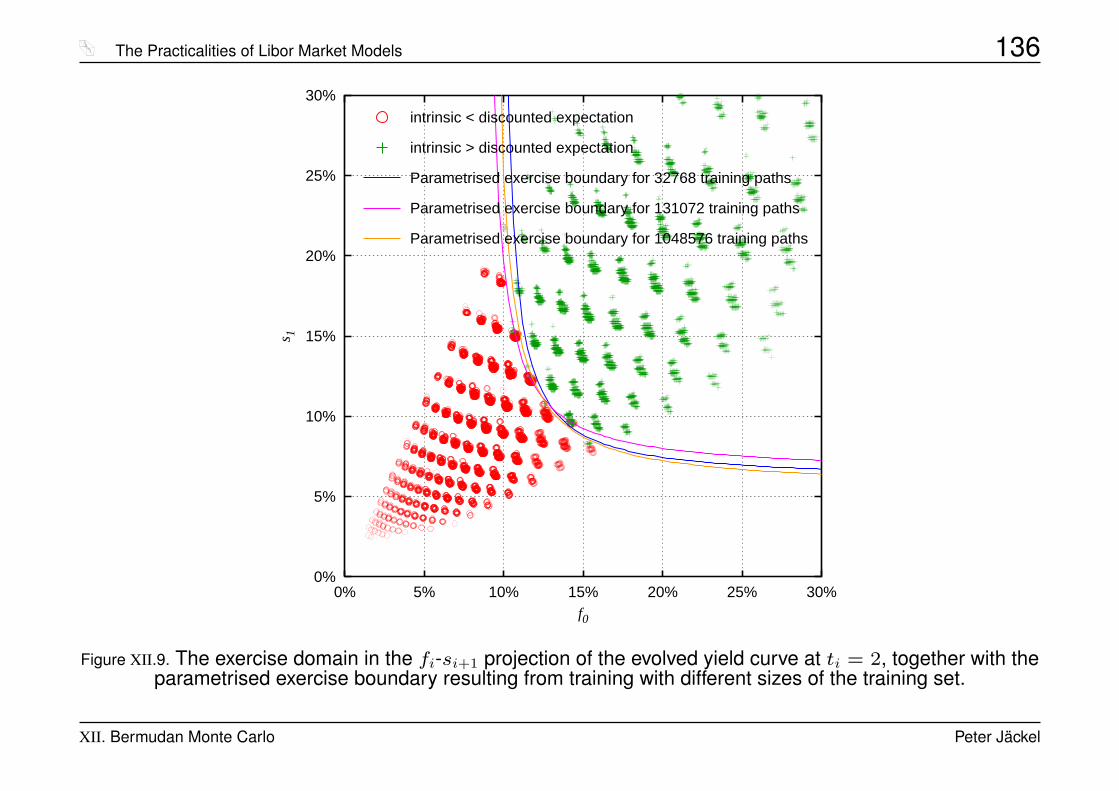
The Practicalities of Libor Market Models 136
0%
5%
10%
15%
20%
25%
30%
0% 5% 10% 15% 20% 25% 30%
s 1
f0
intrinsic < discounted expectation
intrinsic > discounted expectation
Parametrised exercise boundary for 32768 training paths
Parametrised exercise boundary for 131072 training paths
Parametrised exercise boundary for 1048576 training paths
Figure XII.9. The exercise domain in the fi-si+1 projection of the evolved yield curve at ti = 2, together with theparametrised exercise boundary resulting from training with different sizes of the training set.
XII. Bermudan Monte Carlo Peter Jäckel

The Practicalities of Libor Market Models 137
������������������ ��������� ��������� ��������� �������� ������� �������
������������������ ����� ��� ��������� ��������� ��������� �������� ��������
��������� ��������� ��������� ��������� ��������� ��������� �������� ��������
����� ��� ����� ��� ����� ��� ����� ��� ����� ��� ����� ��� ��������� ���������
��������
��������
��������
�������
��������
��������
��������
� � � � ���������� �"!$#%#'&)(+*,!-�/.
0 12435
6"798;:=<)>�?9@�ABDCE@)F8G7"HICJ:LK MN@�M�@)OP 8�7"7
6"798;:=<)>�?9@�AQRCJ@ P 7LSD?98UT C
V-<�8�CJW�7X?9@�ABDCE@)F8G7"HICJ:LK MN@�M�@)OP 8�7"7
V-<�8�CJW�7X?9@�AQRCJ@ P 7LSD?98UT C
Figure XII.10. Bermudan swaption prices from the Monte Carlo model in comparison to those obtained from anon-recombining tree model for a 6-non-call-2 semi-annual payer’s swaption.
XII. Bermudan Monte Carlo Peter Jäckel
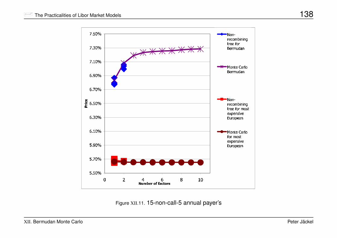
The Practicalities of Libor Market Models 138
���������
��� �����
��� ����
�������
� �����
�������
� �����
� ����
� �������
� � �����
� �������
� � � � � �������������� �"!#!%$�&(')�"�+*
, -. /0
1 2�3"457698 2�:<;�= 3"= 3�>? 5%696A@ 2 5B 6C5 :AD�E�F93
GH2�3 ? 6<I F 5%J 2B 6C5 :AD�E�F93
1 2�3"457698 2�:<;�= 3"= 3�>? 5%696A@ 2 5 :<2�K ?6ML�N�6 3"KM= O 6P"D 5 2 N�6 FC3
GH2�3 ? 6<I F 5%J 2@ 2 5 :A2�K ?6ML�N�6 3"KM= O 6P"D 5 2 N�6 FC3
Figure XII.11. 15-non-call-5 annual payer’s
XII. Bermudan Monte Carlo Peter Jäckel
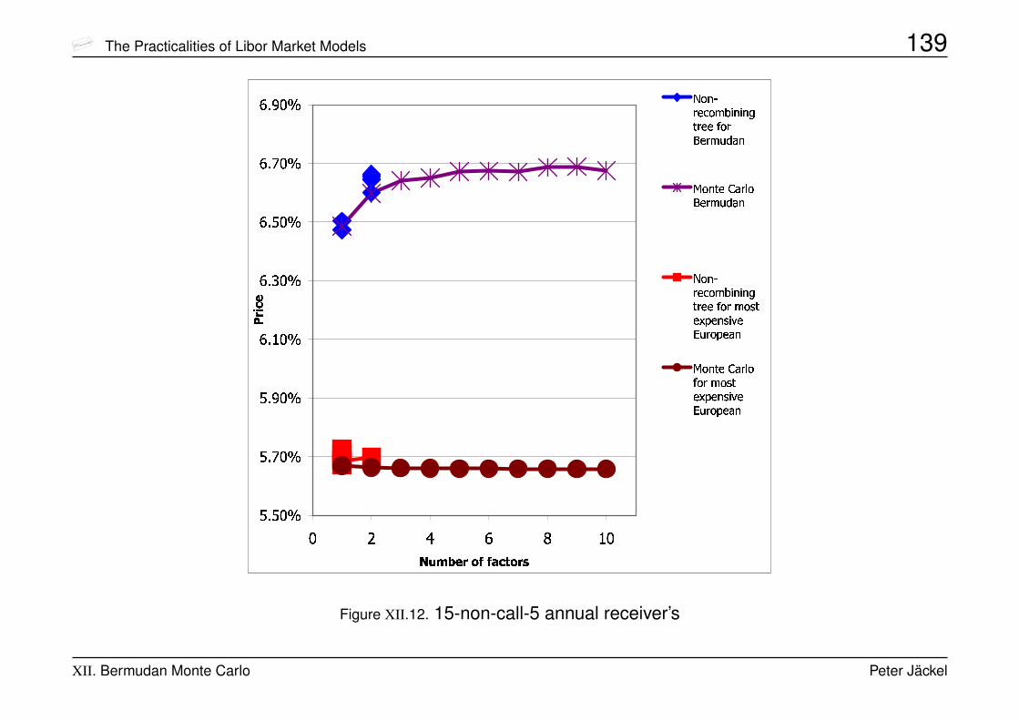
The Practicalities of Libor Market Models 139
���������
���������
���������
������
�� ����
�������
�������
�������
� � � � � �������������� �"!#!%$�&(')�"�+*
, -.0/1
2�354768:9<; 35=?>(@ 47@ 4(AB 8C9<9ED 3 8F 9G8 =EH(I(J<4
KL354 B 9?M J 8CN 3F 9G8 =EH(I(J<4
2�354768:9<; 35=?>(@ 47@ 4(AB 8C9<9ED 3 8 =?35O B9)PRQ(9 47O)@ S 9T7H 8 3 Q(9 JG4KL354 B 9?M J 8CN 3D 3 8 =E35O B9)PRQ(9 47O)@ S 9T7H 8 3 Q(9 JG4
Figure XII.12. 15-non-call-5 annual receiver’s
XII. Bermudan Monte Carlo Peter Jäckel
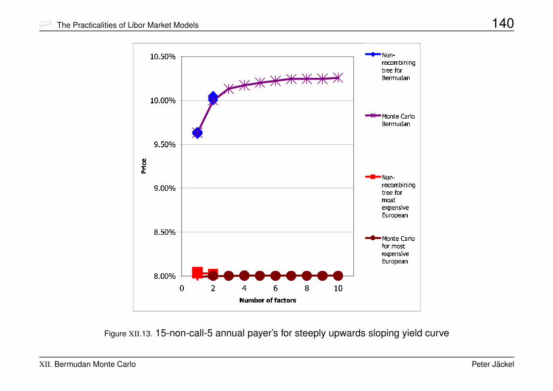
The Practicalities of Libor Market Models 140
���������
��������
��������
�������
� ���������
� ��� ����
� � � � � ��������������! �"�"$#&%(') *�,+
- ./ 01
243�5768 9(: 3�;=<7> 57> 57?@ 8�9A9CB 3 8D 9A8 ;CEF�G(5
HI3�5 @ 9=J G 8�K 3D 9A8 ;CEF�G(5
243�5768 9(: 3�;=<7> 57> 57?@ 8�9A9CB 3 8;=3(L @9NM&O79 57LP> Q 9R7E 8 3 O79 GA5
HI3�5 @ 9=J G 8�K 3B 3 8 ;=3�L @9NM&O79 57LP> Q 9R7E 8 3 O79 GA5
Figure XII.13. 15-non-call-5 annual payer’s for steeply upwards sloping yield curve
XII. Bermudan Monte Carlo Peter Jäckel
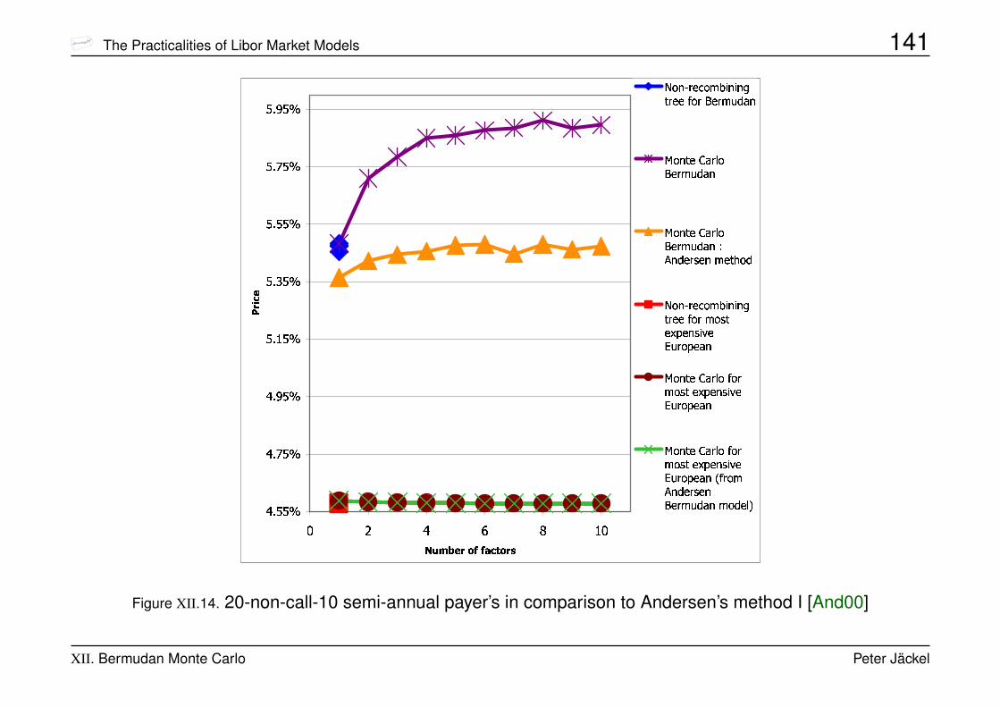
The Practicalities of Libor Market Models 141
��� �����
��� �����
��� �����
�������
��� �����
��� �����
��� �����
��� �����
� � � � ���������������� �!�#"�$&% �'�)(
* +, -.
/10'2�35476�8 0�9;:=< 2�< 2=>? 456�6;@A0'4CBD6�479FE=G=H�2
IJ0'2 ? 6FK!H�45L 0BD6�459;E=G=H�2
IJ0'2 ? 6FK!H�45L 0BD6�459;E=G=H�2NMO�2�G'6�45PQ6�2R9;6 ?TS 0'G
/10'2�35476�8 0�9;:=< 2�< 2=>? 456�6;@A0'4C9F0'P ?6QU�V=6�2�PQ< WD6X�E=470�V=6�H�2
IJ0'2 ? 6FK!H�45L 0�@A0'49;0'P ? 6QU�V=6�2=PY< WD6X�E=470�V=6�H�2
IJ0'2 ? 6FK!H�45L 0�@A0'49;0'P ? 6QU�V=6�2=PY< WD6X�E=470�V=6�H�2RZ&@470�9O�2�G'6�45PQ6�2BD6�459;E=G=H�2R9;0'G=6�L [
Figure XII.14. 20-non-call-10 semi-annual payer’s in comparison to Andersen’s method I [And00]
XII. Bermudan Monte Carlo Peter Jäckel
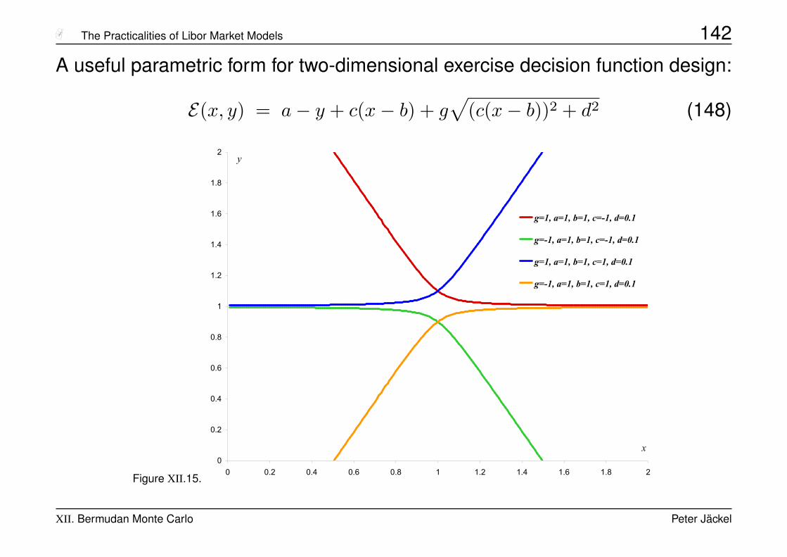
The Practicalities of Libor Market Models 142
A useful parametric form for two-dimensional exercise decision function design:
E(x, y) = a− y + c(x− b) + g√
(c(x− b))2 + d2 (148)
Figure XII.15.
�
���
���
���
���
�
���
���
���
���
�
� ��� ��� ��� ��� � ��� ��� ��� ��� �
�
�
������������������������
������������������������
������������������������
������������������������
XII. Bermudan Monte Carlo Peter Jäckel

The Practicalities of Libor Market Models 143
Hints when computing delta or vega with Bermudan Monte Carlo methods:
• When using an exercise boundary, do not re-optimise the boundary. This isasymptotically correct and reduces the Monte Carlo noise both on delta andvega.
• Better even, if your implementation allows for it, enforce exercise on the same(modified for delta or vega purposes) path at the same point in time [Pit03b]
XII. Bermudan Monte Carlo Peter Jäckel

The Practicalities of Libor Market Models 144
XIII. Cross-currency Libor market modelling
( The formulæ shown in this section are the result of joint work with Atsushi Kawai. )
Define Q(t) as the domestic spot value of one foreign currency unit.
it=t
fiDomestic
today
fi
f
f
t t
t t
n
n
n n+1
n n+1
Domestic
Foreign Foreign
Q
Foreign
Domestic
Figure XIII.1.
In the discretely rolled up money market account measure, the drifts of all do-mestic rates are for a cross-currency Libor market model the same as for asingle currency model, i.e. they are given by equation (41).
XIII. Cross-currency Libor market modelling Peter Jäckel
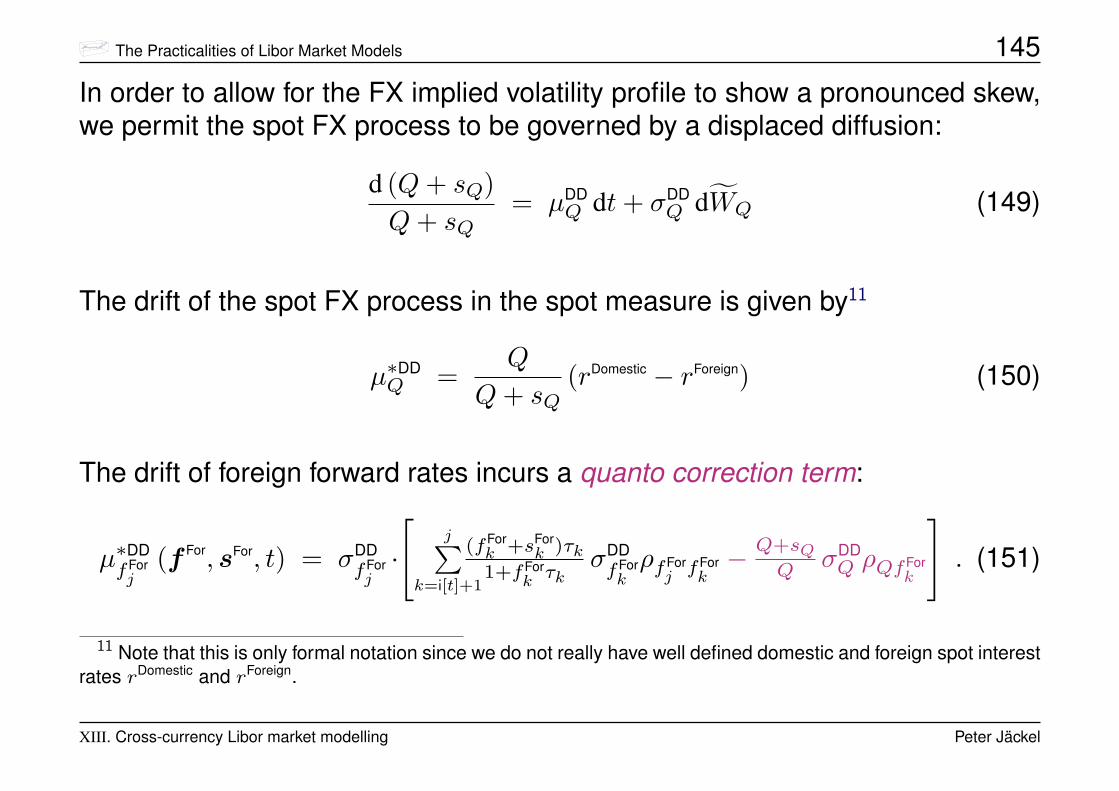
The Practicalities of Libor Market Models 145
In order to allow for the FX implied volatility profile to show a pronounced skew,we permit the spot FX process to be governed by a displaced diffusion:
d (Q+ sQ)Q+ sQ
= µDDQ dt+ σDD
Q dWQ (149)
The drift of the spot FX process in the spot measure is given by11
µ∗DDQ =
Q
Q+ sQ(rDomestic − rForeign) (150)
The drift of foreign forward rates incurs a quanto correction term:
µ∗DDfForj
(f For, sFor, t) = σDDfForj·
[j∑
k=i[t]+1
(fFork +sFor
k )τk1+fFor
kτk
σDDfForkρfFor
j fFork− Q+sQ
Q σDDQ ρQfFor
k
]. (151)
11 Note that this is only formal notation since we do not really have well defined domestic and foreign spot interestrates rDomestic and rForeign.
XIII. Cross-currency Libor market modelling Peter Jäckel
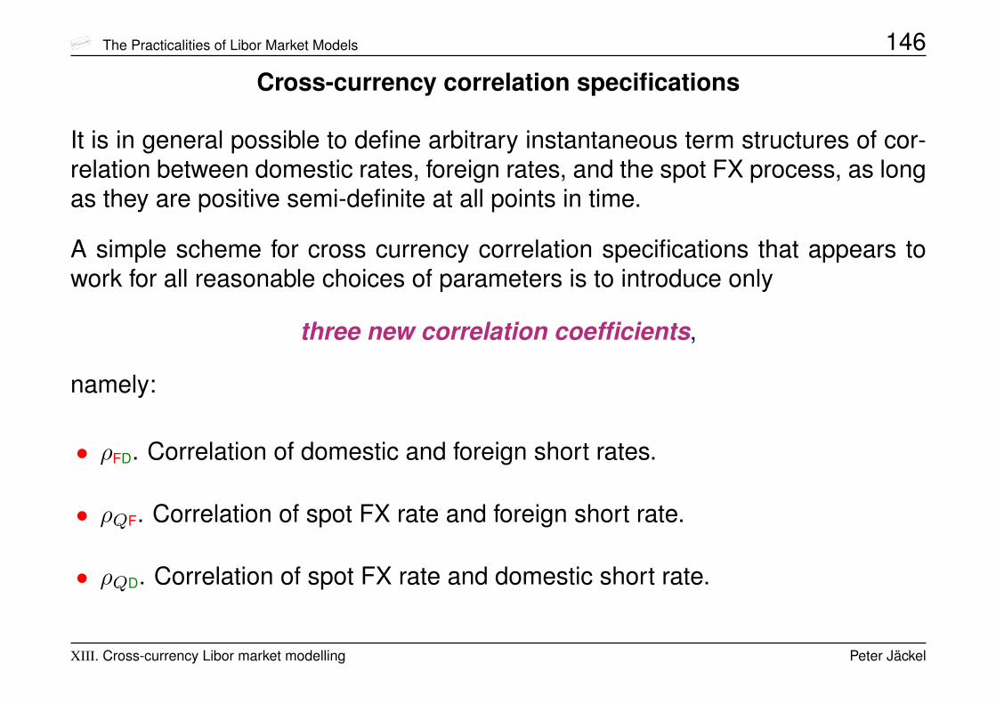
The Practicalities of Libor Market Models 146
Cross-currency correlation specifications
It is in general possible to define arbitrary instantaneous term structures of cor-relation between domestic rates, foreign rates, and the spot FX process, as longas they are positive semi-definite at all points in time.
A simple scheme for cross currency correlation specifications that appears towork for all reasonable choices of parameters is to introduce only
three new correlation coefficients,
namely:
• ρFD. Correlation of domestic and foreign short rates.
• ρQF. Correlation of spot FX rate and foreign short rate.
• ρQD. Correlation of spot FX rate and domestic short rate.
XIII. Cross-currency Libor market modelling Peter Jäckel

The Practicalities of Libor Market Models 147
Then, setρfF
j ,fDk(t) := ρfF
i[t],fFj(t) · ρFD · ρfD
i[t],fDk(t) . (152)
it=t
[t]ifD
[t]if F
today
f
t t
k
k k+1
D
f
t t
j
j j+1
F
fkDf
i[t]D
fi[t]F f
jF
ρ
Foreign
F ρDomestic
D
ρ
Figure XIII.2.
Equally, setρQ,fD
j(t) := ρQD · ρfD
i[t],fDj(t) (153)
andρQ,fF
j(t) := ρQF · ρfF
i[t],fFj(t) . (154)
XIII. Cross-currency Libor market modelling Peter Jäckel
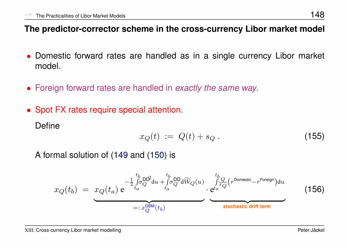
The Practicalities of Libor Market Models 148
The predictor-corrector scheme in the cross-currency Libor market model
• Domestic forward rates are handled as in a single currency Libor marketmodel.
• Foreign forward rates are handled in exactly the same way.
• Spot FX rates require special attention.
DefinexQ(t) := Q(t) + sQ . (155)
A formal solution of (149 and (150) is
xQ(tb) = xQ(ta) e−1
2
tbRta
σDDQ
2du+
tbRta
σDDQ dfWQ(u)
︸ ︷︷ ︸=: xGBM
Q(tb)
· e
tbRta
QxQ
(rDomestic−rForeign)du
︸ ︷︷ ︸stochastic drift term
(156)
XIII. Cross-currency Libor market modelling Peter Jäckel

The Practicalities of Libor Market Models 149
Recall that, in a simplified way, we can view the predictor-corrector scheme asthe approximation of stochastic drift terms by a given frozen state of the yieldcurve, executed twice with different yield curves, and averaged.
For a frozen state of the yield curves and the FX rate,
x> := (xQ, f Domestic> + sDomestic>, f Foreign> + sForeign>) , (157)
the drift term can be re-expressed:
e
tbRta
QxQ
(rDomestic−rForeign)du= e
QxQ
tbRta
(rDomestic−rForeign)du
=
(e
tbRta
(rDomestic−rForeign)du) QxQ
=(P Foreign(x)[ta, tb]P Domestic(x)[ta, tb]
) QxQ
. (158)
XIII. Cross-currency Libor market modelling Peter Jäckel

The Practicalities of Libor Market Models 150
In general, the state-dependent discount factors in equation (158) may have tobe evaluated with the stub formula (36).
The predictor-corrector scheme for the spot FX rate in the cross-currencyLibor market model:
xPredictorQ (tb) = xGBM
Q (tb) ·(P Foreign(x(tb))[ta, tb]P Domestic(x(tb))[ta, tb]
)xQ(ta)−sQxQ(ta)
(159)
xCorrectorQ (tb) = xGBM
Q (tb) ·(P Foreign(x(tb))[ta, tb]P Domestic(x(tb))[ta, tb]
)xQ(tb)−sQxQ(tb)
(160)
xPredictor-CorrectorQ (tb) =
√xPredictorQ (tb) · xCorrector
Q (tb) . (161)
XIII. Cross-currency Libor market modelling Peter Jäckel
The Practicalities of Libor Market Models 151
XIV. Calibration of FX volatilities in a cross-currency Libormarket model
( The formulæ shown in this section have been derived by Atsushi Kawai [KJ07]. )
To fully calibrate a cross-currency Libor market model, both the domestic andthe foreign yield curve must be calibrated first to their respective interest ratemarket information.
The final stage is then the calibration of instantaneous FX factor volatilities suchthat FX plain vanilla option prices meet their respective market values.
XIV. Calibration of FX volatilities in a cross-currency Libor market model Peter Jäckel
The Practicalities of Libor Market Models 152
This last stage is the most difficult one since FX implied volatilities as predictedby the model depend on all of:-
• Levels of both yield curves.
• Volatilities in both currencies’ interest rate markets.
• Correlations within both currencies’ interest rate markets.
• Correlations between the FX factor and both currencies’ interest rate markets.
• FX factor volatilities
Atsushi Kawai [KJ07] derived analytical formulæ for plain vanilla options usingasymptotic aproximations based on Itô-Taylor expansions.
These can be used in a fast root finding procedure to find the term structure ofinstantaneous FX factor volatility that calibrates the model to the market.
XIV. Calibration of FX volatilities in a cross-currency Libor market model Peter Jäckel
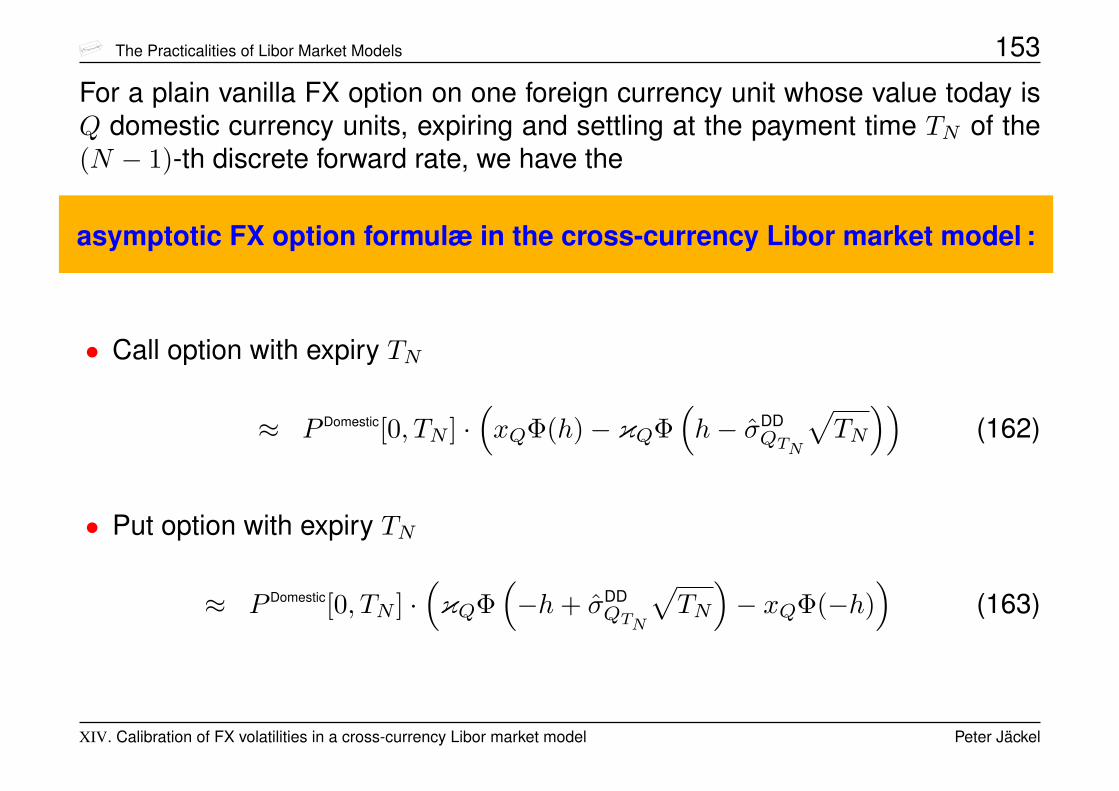
The Practicalities of Libor Market Models 153
For a plain vanilla FX option on one foreign currency unit whose value today isQ domestic currency units, expiring and settling at the payment time TN of the(N − 1)-th discrete forward rate, we have the
asymptotic FX option formulæ in the cross-currency Libor market model :
• Call option with expiry TN
≈ P Domestic[0, TN ] ·(xQΦ(h)− κQΦ
(h− σDD
QTN
√TN
))(162)
• Put option with expiry TN
≈ P Domestic[0, TN ] ·(κQΦ
(−h+ σDD
QTN
√TN
)− xQΦ(−h)
)(163)
XIV. Calibration of FX volatilities in a cross-currency Libor market model Peter Jäckel
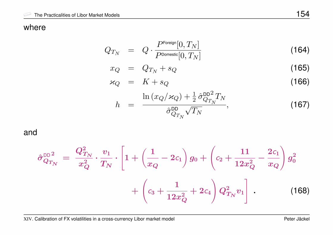
The Practicalities of Libor Market Models 154
where
QTN = Q · PForeign[0, TN ]
P Domestic[0, TN ](164)
xQ = QTN + sQ (165)
κQ = K + sQ (166)
h =ln (xQ/κQ) + 1
2 σDDQTN
2TN
σDDQTN
√TN
, (167)
and
σDDQTN
2 =Q2TN
x2Q
·v1
TN·[1 +
(1
xQ− 2c1
)g0 +
(c2 +
11
12x2Q
−2c1
xQ
)g2
0
+
(c3 +
1
12x2Q
+ 2c4
)Q2TNv1
]. (168)
XIV. Calibration of FX volatilities in a cross-currency Libor market model Peter Jäckel

The Practicalities of Libor Market Models 155
The involved coefficients are defined below. All quantities are defined as seenwith today’s yield curve.
Superscripts (·)D and (·)F stand for domestic and foreign values, respectively.
g0 := QTN −K (169)
γ := 1 +12sQ
(1
QTN+
1Q
)(170)
wDk :=
(f Dk + sD
k) τk1 + f D
kτkyDk := wD · 1− s
Dkτk
1 + f Dkτk
(171)
wFk :=
(f Fk + sF
k) τk1 + f F
kτkyFk := wF · 1− s
Fkτk
1 + f Fkτk
(172)
XIV. Calibration of FX volatilities in a cross-currency Libor market model Peter Jäckel
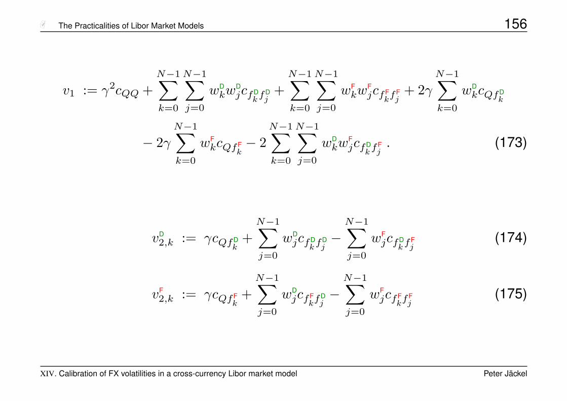
The Practicalities of Libor Market Models 156
v1 := γ2cQQ +N−1∑k=0
N−1∑j=0
wDkw
DjcfD
kfDj
+N−1∑k=0
N−1∑j=0
wFkw
FjcfF
kfFj
+ 2γN−1∑k=0
wDkcQfD
k
− 2γN−1∑k=0
wFkcQfF
k− 2
N−1∑k=0
N−1∑j=0
wDkw
FjcfD
kfFj. (173)
vD2,k := γcQfD
k+N−1∑j=0
wDjcfD
kfDj−N−1∑j=0
wFjcfD
kfFj
(174)
vF2,k := γcQfF
k+N−1∑j=0
wDjcfF
kfDj−N−1∑j=0
wFjcfF
kfFj
(175)
XIV. Calibration of FX volatilities in a cross-currency Libor market model Peter Jäckel

The Practicalities of Libor Market Models 157
vD3,k := −
N−1∑j=k+1
wDjcfD
kfDj
(176)
vF3,k := −γcQfF
k+
k∑j=0
wFjcfF
kfFj−N−1∑j=0
wDjcfF
kfDj
(177)
v4 := γcQQ +N−1∑j=0
wDjcQfD
j−N−1∑j=0
wFjcQfF
j(178)
v5 := −N−1∑j=0
wDjcQfD
j(179)
cQQ :=∫ TN
0
σDDQ
2 (u) du (180)
XIV. Calibration of FX volatilities in a cross-currency Libor market model Peter Jäckel

The Practicalities of Libor Market Models 158
cQfℵk
:=∫ TN
0
σDDQ (u) · ρQfℵ
k(u) · σDD
fℵk(u) du with ℵ ∈ {F,D} (181)
cfℵkfij
:=∫ TN
0
σDDfℵk(u) · ρfℵ
kfij(u) · σDD
fij(u) du with ℵ,i ∈ {F,D} (182)
c1 :=1
2QTNv21
[v2
1 − γ (γ − 1) v24 +
N−1∑k=0
yDk v
D2,k
2 −N−1∑k=0
yFk v
F2,k
2
](183)
c2 := −5c21 + 2g1 + 2g3 + d1 (184)
c3 := 3c21 − 2g1 + 2g2 − 2g3 − d1 + d2 (185)
c4 :=1
2Q2TNv2
1
[γ (γ − 1) v4v5 +
N−1∑k=0
yDkv
D2,kv
D3,k −
N−1∑k=0
yFkv
F2,kv
F3,k
](186)
XIV. Calibration of FX volatilities in a cross-currency Libor market model Peter Jäckel
The Practicalities of Libor Market Models 159
g1 :=1
6Q2TN
(187)
g2 :=1
2Q2TNv2
1
[+ γ (γ − 1) v4 (γcQQ − v4) +
N−1∑k=0
yDk v
D2,k
2 −N−1∑k=0
yFk v
F2,k
2
](188)
g3 :=1
6Q2TNv3
1
[γ (γ − 1) v2
4 ((2γ − 1)v4 − 3v1)
+N−1∑k=0
yDk v
D2,k
2 (3v1 + vD2,k
)−N−1∑k=0
yFk v
F2,k
2 (3v1 + vF2,k
) ](189)
XIV. Calibration of FX volatilities in a cross-currency Libor market model Peter Jäckel
The Practicalities of Libor Market Models 160
d1 :=1
Q2TNv3
1
[v3
1 + γ2 (γ − 1)2v2
4cQQ − 2γ (γ − 1) v1v24
+ 2v1
N−1∑k=0
(yDk v
D2,k
2 − yFk v
F2,k
2)
(190)
− 2γ (γ − 1) v4
N−1∑k=0
(yDkv
D2,kcQfD
k− yF
kvF2,kcQfF
k
)
+N−1∑j=0
N−1∑k=0
(ωDDjk − 2ωD F
jk + ωF Fjk
) ]
ωℵijk := yℵj · vℵ2,j · cfℵj fi
k· vi
2,k · yik with ℵ,i ∈ {F,D} (191)
XIV. Calibration of FX volatilities in a cross-currency Libor market model Peter Jäckel
The Practicalities of Libor Market Models 161
d2 :=1
2Q2TNv2
1
[v2
1 + γ2 (γ − 1)2c2QQ − 2γ (γ − 1) v2
4
+N−1∑k=0
(yDk v
D2,k
2 − yFk v
F2,k
2)− γ (γ − 1)
N−1∑k=0
(yDkc
2QfD
k− yF
kc2QfF
k
)
+N−1∑k=0
N−1∑j=0
(yDjc
2fDj f
DkyDk − 2yD
jc2fDj f
FkyFk + yF
jc2fFj f
FkyFk
)](192)
Finally: some numerical results showing the accuracy of the analytical formulæby comparison with Monte Carlo valuations.
XIV. Calibration of FX volatilities in a cross-currency Libor market model Peter Jäckel
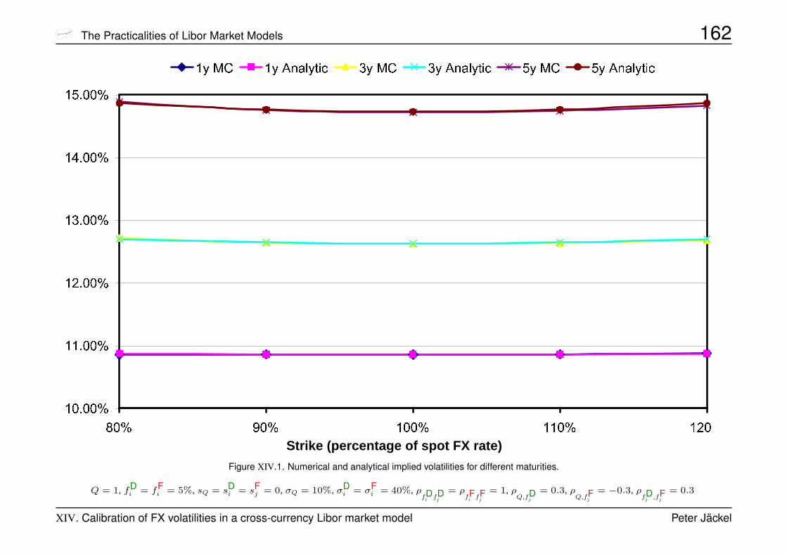
The Practicalities of Libor Market Models 162
Strike (percentage of spot FX rate)
Figure XIV.1. Numerical and analytical implied volatilities for different maturities.
Q = 1, fDi = fF
i = 5%, sQ = sDi = sF
j = 0, σQ = 10%, σDi = σF
i = 40%, ρfDi fDj
= ρfFi fFj
= 1, ρQ,fDj
= 0.3, ρQ,fFj
= −0.3, ρfDj ,fFj
= 0.3
XIV. Calibration of FX volatilities in a cross-currency Libor market model Peter Jäckel
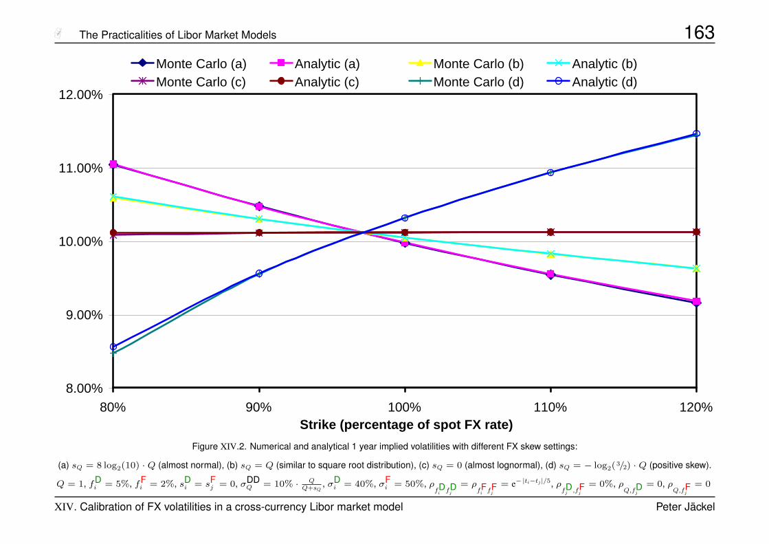
The Practicalities of Libor Market Models 163
8.00%
9.00%
10.00%
11.00%
12.00%
80% 90% 100% 110% 120%Strike (percentage of spot FX rate)
Monte Carlo (a) Analytic (a) Monte Carlo (b) Analytic (b)Monte Carlo (c) Analytic (c) Monte Carlo (d) Analytic (d)
Figure XIV.2. Numerical and analytical 1 year implied volatilities with different FX skew settings:
(a) sQ = 8 log2(10) ·Q (almost normal), (b) sQ = Q (similar to square root distribution), (c) sQ = 0 (almost lognormal), (d) sQ = − log2(3/2) ·Q (positive skew).
Q = 1, fDi = 5%, fF
i = 2%, sDi = sF
j = 0, σDDQ = 10% · Q
Q+sQ, σD
i = 40%, σFi = 50%, ρ
fDi fDj= ρ
fFi fFj= e−|ti−tj |/5, ρ
fDj ,fFj= 0%, ρ
Q,fDj= 0, ρ
Q,fFj= 0
XIV. Calibration of FX volatilities in a cross-currency Libor market model Peter Jäckel
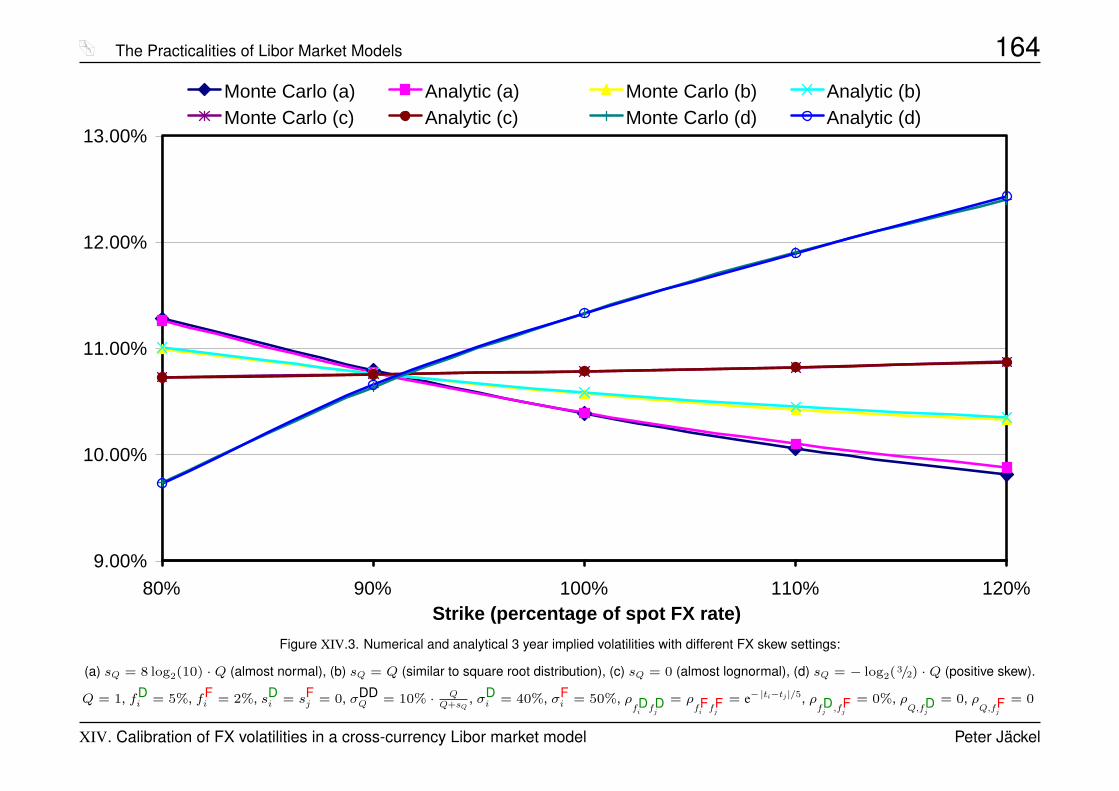
The Practicalities of Libor Market Models 164
9.00%
10.00%
11.00%
12.00%
13.00%
80% 90% 100% 110% 120%Strike (percentage of spot FX rate)
Monte Carlo (a) Analytic (a) Monte Carlo (b) Analytic (b)Monte Carlo (c) Analytic (c) Monte Carlo (d) Analytic (d)
Figure XIV.3. Numerical and analytical 3 year implied volatilities with different FX skew settings:
(a) sQ = 8 log2(10) ·Q (almost normal), (b) sQ = Q (similar to square root distribution), (c) sQ = 0 (almost lognormal), (d) sQ = − log2(3/2) ·Q (positive skew).
Q = 1, fDi = 5%, fF
i = 2%, sDi = sF
j = 0, σDDQ = 10% · Q
Q+sQ, σD
i = 40%, σFi = 50%, ρ
fDi fDj= ρ
fFi fFj= e−|ti−tj |/5, ρ
fDj ,fFj= 0%, ρ
Q,fDj= 0, ρ
Q,fFj= 0
XIV. Calibration of FX volatilities in a cross-currency Libor market model Peter Jäckel

The Practicalities of Libor Market Models 165
10.00%
11.00%
12.00%
13.00%
14.00%
80% 90% 100% 110% 120%Strike (percentage of spot FX rate)
Monte Carlo (a) Analytic (a) Monte Carlo (b) Analytic (b)Monte Carlo (c) Analytic (c) Monte Carlo (d) Analytic (d)
Figure XIV.4. Numerical and analytical 5 year implied volatilities with different FX skew settings:
(a) sQ = 8 log2(10) ·Q (almost normal), (b) sQ = Q (similar to square root distribution), (c) sQ = 0 (almost lognormal), (d) sQ = − log2(3/2) ·Q (positive skew).
Q = 1, fDi = 5%, fF
i = 2%, sDi = sF
j = 0, σDDQ = 10% · Q
Q+sQ, σD
i = 40%, σFi = 50%, ρ
fDi fDj= ρ
fFi fFj= e−|ti−tj |/5, ρ
fDj ,fFj= 0%, ρ
Q,fDj= 0, ρ
Q,fFj= 0
XIV. Calibration of FX volatilities in a cross-currency Libor market model Peter Jäckel
The Practicalities of Libor Market Models 166
References[AA00] L. Andersen and J. Andreasen. Volatility Skews and Extensions of the Libor Market Model. Applied Mathematical Finance,
7(1):1–32, March 2000.[Alb72] A. Albert. Regression and the Moore-Penrose Pseudo-Inverse. Academic Press, 1972.[And00] L. Andersen. A simple approach to the pricing of Bermudan swaptions in the multifactor LIBOR market model. Journal of
Computational Finance, 3(2):5–32, Winter 1999/2000.[BD96] M. Broadie and J. Detemple. American Option Valuation: New Bounds, Approximations, and a Comparison of Existing Meth-
ods. Review of Financial Studies, 9(4):1211–1250, 1996.[Bec80] S. Beckers. The constant elasticity of variance model and its implications for option pricing. Journal of Finance, XXXV(3):661–
673, June 1980.[BG97a] M. Broadie and P. Glasserman. Monte Carlo methods for pricing high-dimensional American options: An overview. Net
Exposure: The Electronic Journal of Financial Risk, 1(3):15–37, December 1997.[BG97b] M. Broadie and P. Glasserman. Pricing American-Style Securities Using Simulation. Journal of Economic Dynamics and
Control, 21(8–9):1323–1352, 1997.[CIR81] J. C. Cox, J. E. Ingersoll, and S. A. Ross. The relation between forward prices and futures prices. Journal of Financial
Economics, 9(4):321–346, December 1981.[CR76] J. C. Cox and S. A. Ross. The valuation of options for alternative stochastic processes. Journal of Financial Economics,
3:145–166, March 1976.[GZ99] P. Glasserman and X. Zhao. Fast greeks by simulation in forward Libor models. Journal of Computational Finance, 3(1):5–39,
Fall 1999.[HP81] J. M. Harrison and S. Pliska. Martingales and stochastic integrals in the theory of continuous trading. Stochastic processes
and their applications, 11:215–260, 1981.[Jäc02] P. Jäckel. Monte Carlo methods in finance. John Wiley and Sons, February 2002.[Jäc03] P. Jäckel. Mind the Cap. Wilmott, pages 54–68, September 2003. www.jaeckel.org/MindTheCap.pdf.[JK05] P. Jäckel and A. Kawai. The Future is Convex. Wilmott, pages 2–13, February 2005. www.jaeckel.org/
TheFutureIsConvex.pdf.
References Peter Jäckel

The Practicalities of Libor Market Models 167[JL03] S. Johnson and H. Lee. Capturing the Smile. Risk, 16(3), March 2003. www.numerix.com/news/announcements/0303_
smile.pdf.[JR00] P. Jäckel and R. Rebonato. The link between caplet and swaption volatilities in a Brace-Gatarek-Musiela/Jamshidian frame-
work: approximate solutions and empirical evidence. Journal of Computational Finance, 6(4):41–59, 2003 (submitted in 2000).www.jaeckel.org/LinkingCapletAndSwaptionVolatilities.pdf.
[JT02] M. Joshi and J. Theis. Bounding Bermudan swaptions in a swap-rate market model. Quantitative Finance, 2(5):370–377,October 2002. www.quarchome.org/BermBounds.pdf.
[Kaw02] A. Kawai. Analytical and Monte Carlo swaption pricing under the forward swap measure. Journal of Computational Finance,6(1):101–111, 2002. www.maths.unsw.edu.au/statistics/files/preprint-2002-12.pdf.
[Kaw03] A. Kawai. A new approximate swaption formula in the LIBOR market model: an asymptotic expansion approach. Applied Math-ematical Finance, 10(1):49–74, March 2003. www.maths.unsw.edu.au/statistics/files/preprint-2002-13.pdf.
[KJ07] A. Kawai and P. Jäckel. An asymptotic FX option formula in the cross currency Libor marketmodel. Wilmott, pages 74–84, March 2007. First published in October 2006 at www.jaeckel.org/AnAsymptoticFXOptionFormulaInTheCrossCurrencyLiborMarketModel.pdf.
[KN97] G. Kirikos and D. Novak. Convexity Conundrums. Risk, pages 60–61, March 1997. www.powerfinance.com/convexity.[KS91] I. Karatzas and S. E. Shreve. Brownian motion and Stochastic Calculus. Springer, 1991.[KS98] I. Karatzas and S. E. Shreve. Methods of Mathematical Finance. Springer, 1998.[LLS] A. Lumsdaine, L. Lee, and J. Siek. The iterative template library. www.osl.iu.edu/research/itl.[LS98] F. A. Longstaff and E. S. Schwartz. Valuing American options by simulation: A simple least squares approach. Working paper,
The Anderson school, UCLA, 1998.[Mat01] K. Matsumoto. Lognormal swap approximation in the Libor marekt model and its application. Journal of Computational
Finance, 5(1):107–131, 2001.[Mey03a] M. Meyer. Monte Carlo Pricing of Bermudan Options. martingale.berlios.de/topics/Bermudan/Index.html, 2003.[Mey03b] M. Meyer. Monte Carlo simulation with Java and C++. download.berlios.de/martingale/MCBook-1.2.pdf.gz,
2003. download.berlios.de/martingale/MCBook-1.2.pdf.gz.[Pit03a] V. Piterbarg. A Stochastic Volatility Forward Libor Model with a Term Structure of Volatility Smiles. Technical report, Bank of
America, 2003. ssrn.com/abstract=472061.
References Peter Jäckel
The Practicalities of Libor Market Models 168[Pit03b] V. Piterbarg. Computing deltas of callable Libor exotics in forward Libor models. Journal of Computational Finance, 7(3), 2003.
ssrn.com/abstract=396180.
[Pit03c] V. Piterbarg. Mixture of Models: A Simple Recipe for a ... Hangover ? Technical report, Bank of America, 2003. ssrn.com/abstract=393060.
[PTVF92] W. H. Press, S. A. Teukolsky, W. T. Vetterling, and B. P. Flannery. Numerical Recipes in C. Cambridge University Press, 1992.www.library.cornell.edu/nr/cbookcpdf.html.
[PvR05] R. Pietersz and M. van Regenmortel. Generic Market Models. Technical report, ABN AMRO, January 2005. ssrn.com/abstract=605301.
[Rub83] M. Rubinstein. Displaced diffusion option pricing. Journal of Finance, 38:213–217, March 1983.
[Sch89] M. Schroder. Computing the Constant Elasticity of Variance Option Pricing Formula. Journal of Finance, 44(1):211–219,March 1989. home.ust.hk/jinzhang/ust/Schroder_JF.pdf.
[Sch02] E. Schlögl. A multicurrency extension of the lognormal interest rate market models. Finance and Stochastics, 6:173–196,2002.
[Sob79] I. M. Sobol’. On the Systematic Search in a Hypercube. Siam J. Numer. Anal., 16(5), October 1979.
[Wu03] L. Wu. Fast at-the-money calibration of the Libor market model using Lagrange multipliers. Journal of Computational Finance,6(2):39–72, Winter 2002/2003.
References Peter Jäckel