Embed Size (px)
Citation preview
Volume 7/Number 1, Fall 2003 URL: www.thejournalofcomputationalfinance.com
This paper develops formulas for pricing caps and swaptions in Libor market models with jumps. The arbitrage-free dynamics of this class of models were characterized in Glasserman and Kou (2003) in a framework allowing for very general jump processes. For computational purposes, it is convenient to model jump times as Poisson processes; however, the Poisson property is not preserved under the changes of measure commonly used to derive prices in the Libor market model framework. In particular, jumps cannot be Poisson under both a forward measure and the spot measure, and this complicates pricing. To develop pricing formulas, we approximate the dynamics of a forward rate or swap rate using a scalar jump-diffusion process with time-varying parameters. We develop an exact formula for the price of an option on this jump-diffusion through explicit inversion of a Fourier transform. We then use this formula to price caps and swaptions by choosing the parameters of the scalar diffusion to approximate the arbitrage-free dynamics of the underlying forward or swap rate. We apply this method to two classes of models: one in which the jumps in all forward rates are Poisson under the spot measure, and one in which the jumps in each forward rate are Poisson under its associated forward measure. Numerical examples demonstrate the accuracy of the approximations.
1 Introduction
This paper develops formulas for pricing caps and swaptions in jump-diffusion Libor market models. The success of the original Libor market models and their extensions (including Brace, Gatarek, and Musiela, 1997; Miltersen, Sandmann, and Sondermann, 1997; Jamshidian, 1997; Andersen and Andreasen, 2000; Joshi and Rebonato, 2001; and Zühlsdorff, 2000) is due in part to the availability of formulas and fast numerical methods for pricing caps and swaptions within this framework. These are necessary for model calibration. The Libor market model framework was extended to include jumps in Glasserman and Kou (2003) and, using a different approach, in Jamshidian (1999). Glasserman and Kou (2003) focus on characterizing the arbitrage-free dynamics of forward rates in the
Cap and swaption approximations in Libor market models with jumps
Paul Glasserman403 Uris Hall, Graduate School of Business, Columbia University, New York, NY 10027
Nicolas MerenerDepartment of Applied Physics and Applied Mathematics, Columbia University, New York, NY
10027
The authors thank Professor Steve Kou for helpful discussions in developing the approxima-tions in this paper. This work is supported by NSF grant DMS0074637.
URL: thejournalofcomputationalfinance.com Journal of Computational Finance
Paul Glasserman and Nicolas Merener2
presence jumps. They identify a tractable subclass of models in which caplet prices are given through a blending of the formulas of Black (1976) and Merton (1976), but they leave open the question of simultaneous pricing of swaptions and also the question of cap and swaption pricing for other specifications of the jump process. We take up these questions here.
Including jumps in a model of the Libor term structure introduces an issue not present in purely diffusive models: the most convenient model of jumps is a Poisson process, but the Poisson property is not preserved by the changes of measure (eg, between the spot measure, the forward measure, and the swap measure) that lie at the heart of the market model framework. In formulating a model, one must choose the measure under which jumps will be Poisson. Glasserman and Kou (2003) obtain a caplet formula by requiring that each Libor rate have Poisson jumps under its associated forward measure; we refer to this choice here as a forward Poisson (FP) specification. For other purposes, it may be desirable to have jumps in all forward Libor rates follow Poisson processes simultaneously under a single measure, so here we also consider cap and swap-tion prices in a spot Poisson (SP) specification that accomplishes this under the spot measure. The arbitrage-free dynamics of forward Libor under both specifi-cations follow immediately from more general results in Glasserman and Kou (2003).
Because we consider cap and swaption prices in both the SP and FP specifica-tions, we deal with four basic pricing problems. Our strategy for all four cases may be summarized as follows:
❑ Express the option (caplet or swaption) as an expectation involving only a single underlying rate (forward rate or swap rate) through appropriate choice of measure (forward measure or swap measure).
❑ Approximate the dynamics of the underlying rate under the chosen measure using a scalar jump-diffusion with time-varying parameters, Poisson jump times, and lognormal jump-size factors.
❑ Apply an extension of Merton’s (1976) formula to value an option on the approximating jump-diffusion process.
We comment briefly on each of these steps. The first uses ideas now standard in the market model literature; we review these in Section 2. In the last step, the extension is needed to handle time-varying parameters. The approximating jump-diffusion process has the property that its logarithm has independent incre-ments, and this lends itself to option pricing through Fourier transform inversion. We obtain an option pricing result by inverting the transform explicitly. This for-mula is the key to our cap and swaption approximations. The formula could also be used to incorporate jumps in the pricing of equity or currency options.
In the three-step strategy outlined above, only the second step involves approximations – the first and third are exact. To approximate a more general process (forward rate or swap rate) using a simpler jump-diffusion, we need,
Volume 7/Number 1, Fall 2003 URL: www.thejournalofcomputationalfinance.com
Cap and swaption approximations in Libor market models with jumps 3
in each case, to choose the approximating drift, diffusion coefficient, Poisson arrival rate, and jump-size parameters. We do this by analyzing the dynamics of forward rates and swap rates under the appropriate measures.
The presence of jumps suggests that we are working in an incomplete market and thus raises the question of the sense in which a formula can legitimately be interpreted as a price. We are, in effect, assuming that the market is made “nearly” complete by derivative prices. Because caps and swaptions are actively traded, the purpose of pricing formulas lies in calibrating model parameters (such as jump rates) to market prices – the formulas are most useful in reverse. In a complete market, the prices of derivatives would completely determine the parameters; in practice, we expect that market prices would substantially constrain though not completely determine parameter values. The remaining indeterminacy would be removed by imposing additional restrictions on the parameterization. This is standard practice in, for example, calibrating a diffu-sion model to a volatility surface.
The rest of the paper is organized as follows. Section 2 reviews Libor market models and discusses derivatives pricing and changes of numeraire. Section 3 introduces an exact formula for the price of a European option on a particu-lar type of jump-diffusion with time-varying coefficients. Section 4 discusses general arbitrage restrictions on market models with jumps, and the dynamics under relevant pricing measures. In Section 5, we develop caplet and swaption formulas in the SP specification and support the method through numerical experiments. We treat the FP specification in Section 6. By construction, caplets are priced exactly in this setting, but we go beyond Glasserman and Kou (2003) in allowing for time-varying parameters. We derive a swaption approximation and support it through numerical results. Section 7 summarizes the models and formulas presented. All proofs are collected in the Appendix.
2 Libor market models and derivatives
We consider Libor market models of the term structure, of the type developed by Brace, Gatarek, and Musiela (1997); Miltersen, Sandmann, and Sondermann (1997); and Jamshidian (1997). We take a discrete tenor structure – a finite set of dates 0 = T0 < T1 < … < TM + 1, with Ti + 1 – Ti ≡ δ. The fixed accrual period δ is expressed as a fraction of a year; for instance, δ = 1 ⁄ 2 represents six months. Each tenor date Tk is the maturity of a zero-coupon bond; Bk (t ) denotes the price of that bond at time t ∈[0, Tk] and Bk (Tk) ≡ 1. Forward Libor rates L1,…, LM may be defined from the bond prices by setting
(1)L tB t
B tt T k Mk
k
kk( )
( )
( ), [ , ] , , ,= −
⎛
⎝⎜
⎞
⎠⎟ ∈ = …
+
11 0 1
1δ
Similarly, L0(0) is the rate for [0, T1]. Let η(t ) = inf{ j ≥ 0: Tj ≥ t} so that η(t ) is the index of the next maturity as of time t. Bond prices can then be written in terms of Libor rates and the next bond to mature Bη (t ) as
URL: thejournalofcomputationalfinance.com Journal of Computational Finance
Paul Glasserman and Nicolas Merener4
(2)B t B tL tk t
jj t
k
( ) ( )( )( )
( )
=+=
−
∏ηη δ
1
1
1
Absence of arbitrage by trading in bonds is essentially equivalent to the existence of a numeraire M(t ) and an associated measure under which dis-counted asset prices Bj (t ) ⁄M(t ) are martingales. For a general class of payoffs, determined by the state of the set of forward rates at time T, the price C(0) of a contingent claim with payoff C(T ) becomes
C MC T
M T( ) ( )
( )
( )0 0= ⎡
⎣⎢⎤⎦⎥
E
the expectation taken with respect to the measure associated with numeraire M(t ). There are several numeraires that have been shown to be convenient in the pricing of derivatives. The spot martingale measure P, introduced by Jamshidian (1997), uses a discretely compounded money market account as numeraire,
(3)B t B t L tt jj
t
( ) ( ) ( )( )
( )
= +( )=
−
∏η
η
δ10
1
Under this measure, the price of a caplet with strike K, for the period [Tn, Tn + 1], which pays δ (Ln(Tn) – K) + at time Tn + 1 is
CL T
L T KnP
j jj
n
n n( )( )
( )01
10
=+
−( )⎡
⎣⎢⎢
⎤
⎦⎥⎥=
+∏δδ
E
For pricing derivatives tied to just one forward rate (such as a caplet), it is often convenient to choose as numeraire a zero-coupon bond maturing at the end of the accrual period associated with the forward rate. Thus, to price a claim con-tingent on Ln, we take as numeraire the bond Bn + 1. Observe from (1) that
δL tB t B t
B tnn n
n( )
( ) ( )
( )=
− +
+
1
1
is the ratio of a portfolio of assets to Bn + 1(t), so that under the measure asso-ciated with Bn + 1 as numeraire, Ln(t ) is a martingale. This in fact is why this particular choice of numeraire is convenient. The measure associated with this numeraire is usually called the forward measure or terminal measure for matu-rity Tn + 1; see Musiela and Rutkowski (1997) for background. Writing EPn + 1 for expectation under this measure, we have
(4)C B L T Kn nP
n nn
( ) ( ) ( )0 011
= −( )[ ]+++
δ E
The nth caplet price is thus determined by the dynamics of Ln under its associ-ated forward measure.
Volume 7/Number 1, Fall 2003 URL: www.thejournalofcomputationalfinance.com
Cap and swaption approximations in Libor market models with jumps 5
Swaptions are also widely traded derivatives. A payer’s swaption maturing at Tn is an option to enter a fixed-for-floating swap between dates Tn and TM + 1. If the option is exercised, the holder makes fixed payments δK and receives float-ing payments δLi (Ti ) at Ti + 1, i = n,…, M. The swaption value at expiration is
C T B T S T Kn M n jj n
M
n n M n, ,( ) ( ) ( )= −( )+=
+∑δ 1
where the swap rate Sn, M is
(5)S t b t L t b tB t
B tn M j j
j n
M
jj
ji n
M, ( ) ( ) ( ) ( )( )
( )≡ ≡
=
+
+=
∑ ∑with
1
1
The time-0 swaption price under the spot martingale measure is
(6)C B T S T Kn MP
jj n
M
n n M n, ,( ) ( ) ( )0 1= −( )⎡
⎣⎢
⎤
⎦⎥+
=
+∑δE
but it is often convenient to change the pricing measure and take, as Jamshidian (1997) did,
(7)M t B tj
j n
M
( ) ( )= +=∑δ 1
as numeraire, associated to the measure Pn, M. This leads to an alternative rep-resentation for the swaption price, as the deterministically discounted expected value of a European payoff,
(8)C B S T Kn M jj n
MP
n M nn M
, ,( ) ( ) ( ),
0 01= −( )[ ]+=
+∑δ E
Furthermore, from the representation,
S tB t B t
B tn M
n M
jj n
M, ( )( ) ( )
( )=
− +
+=∑1
1δ
and the form of the numeraire in (7), it is evident that Sn, M is a martingale under Pn, M.
We have seen that, under the appropriate changes of measure, both caplets and swaptions become European options with trivial discounting, on forward and swap rates respectively. This naturally suggests a strategy to develop pricing formulas. The idea is to approximate the dynamics of each of the relevant rates, under the corresponding pricing measure, by dynamics simple enough to lead to formulas for option prices. To carry this out, in the section we develop an option
URL: thejournalofcomputationalfinance.com Journal of Computational Finance
Paul Glasserman and Nicolas Merener6
pricing formula for relatively simple scalar jump-diffusion. This formula will then be the tool we use to develop cap and swaption pricing formulas.
3 A jump-diffusion option formula
In this section, we digress from our discussion of term structure models to develop our key pricing tool. We consider the pricing of a European option on a scalar jump-diffusion with Poisson jump times and lognormal jump-size factors. This is a process used by Merton (1976) to model a stock price, except that we allow the parameters of the model to vary with time. This extension is essential for our intended application. We restrict the time dependence of the coefficients by allowing them to change only at tenor dates while remaining constant dur-ing each accrual period. This restriction is computationally convenient and consistent with the way interest rate volatilities are calibrated in practice. One could presumably extend the pricing formula below to continuously varying para-meters by appropriately replacing the sums with integrals.
Consider, then, the process
(9)d
(d d d
G t
G ta t t t W t Y t Tj
j
N t
M( )
)( ) ( ) ( ) ( ) ,
( )
−= + + −
⎛
⎝⎜⎜
⎞
⎠⎟⎟ ≤ ≤
=∑γ 1 0
1
with W(t ) a standard Brownian motion, γ (t ) deterministic and bounded, N a Poisson process with rate λ(t ), and Yj ∈(0, ∞) independent with lognormal density f ( · , t) having mean 1 + m (t ), and with W, N, and {Y1, Y2,…,} mutually independent. We take the G to be right-continuous and denote by G(t–) the left limit at t. As the marks Yj are positive, the form of the jump term ensures that G(t ) also remains positive, given positive G(0) . We parameterize each lognor-mal density f ( · , t ) through the mean µ (t ) and standard deviation σ (t ) of the associated normal density. In particular, m = eµ + σ2⁄ 2 – 1. By piecewise constant coefficients we mean that a(t ) = ak, γ (t ) = γk, λ (t ) = λ k and f (y, t ) = fk(y) for Tk–1 < t ≤ Tk, k = 1,…, M. At this point, G has no specific financial meaning; later, we use it to model or approximate a forward rate or a swap rate.
Imposing a piecewise constant parameterization on dynamics (9) leads to closed form European option prices through the Fourier transform approach, successfully used to price contingent claims by Heston (1993); Duffie, Pan, and Singleton (2000); Carr and Madan (1999); and Scott (1997) among others. The Fourier inversion approach is based on the transform of the logarithm of the asset (G in our case) defined as
ψ( ) , log( ( ))z zz G t≡ [ ] ∈E e �
In particular, we need the existence, in analytic form, of ψ (z) at z = 1 + iu and z = iu, with u ∈� and i = ��–1. The choice of a lognormal jump density f is standard in financial modeling and is also computationally convenient. The same method could be used with other choices of f; Kou (1999) uses a double- exponential distribution for log jump sizes. The key point is that the logarithm
Volume 7/Number 1, Fall 2003 URL: www.thejournalofcomputationalfinance.com
Cap and swaption approximations in Libor market models with jumps 7
of G has independent increments and piecewise constant coefficients, so its dis-tribution is given by a convolution and is thus convenient for transform analysis. The pricing formula for a European option maturing at Tn, n ≤ M, is as follows:
PROPOSITION 3.1 With G defined as in (9), the expected value of a European payoff is
(10)E ( ( )) ) ( )G T K G Kn −[ ] = −+ 0 1 2Π Π
with
(11)
(12)
Π
Π
1
2 0
0
2
4 0
0
1
2
1
1
2
1
1
3
= +− ( )( )
= +− ( )( )
∞
∞
∫
∫
π
π
ed
ed
B u KG
B u KG
B u u
uu
B u u
uu
( )( )
( )( )
sin ( ) log
sin ( ) log
where wi = µi + σi2, αi = ai – γi
2 ⁄ 2 and
B u w u m u
B u w u u u
B u u
iu
i i i ii
n
iu
i i ii
n
iu
i
i i
i i
i
11 2 2 2
1
21 2 2
1
32
2 2
2 2
2 2
1 2( ) cos( )
( ) sin( )
( ) cos( )
( )
( )
= −[ ] − −
= + +
= −
+ −
=
+ −
=
−
∑
∑
δ λ λ γ
δ λ α γ
δ λ µ
µ σ
µ σ
σ
e
e
e 11 22 2
1
42
1
2 2
[ ] −
= +
=
−
=
∑
∑
γ
δ λ µ ασ
ii
n
iu
i ii
n
u
B u u ui( ) sin( )e
This result is proved in the Appendix. The integrals in (11) and (12) can be computed to very high accuracy in very short time, so the result is essentially a closed-form expression.
In allowing time-varying coefficients, the formula above extends the Merton formula (1976) for the price of a European option on a lognormal jump- diffusion. The Merton formula was used by Glasserman and Kou (2003) (in a manner analogous to the use of the Black, 1976, formula in Brace, Gatarek and Musiela, 1997) to build a jump-diffusion model that prices caplets (or swap-tions) exactly by forcing the forward (or swap) rate to be, under its own forward (or swap) measure, a scalar lognormal jump-diffusion with Poisson distributed jump times and constant coefficients over the life of the rate. In the spirit of Glasserman and Kou we obtain Proposition 3.1 as an exact caplet pricing for-mula for those model specifications in which the dynamics of a forward rate under its forward measure are exactly of the form (9). Proposition 3.1 is also
URL: thejournalofcomputationalfinance.com Journal of Computational Finance
Paul Glasserman and Nicolas Merener8
potentially useful for equity and currency options, where jumps can be used to reproduce a skew in implied volatilities.
Although we do not pursue this line in this paper, we could also build models, with piecewise constant coefficients, that price swaptions exactly through Proposition 3.1. However, as noted by Glasserman and Kou (2003), and as will become clear later from the dynamics of the rates under different measures, exact prices cannot be achieved for caplets and swaptions within the same model specification, because the law of the jumps cannot be Poisson under both for-ward and swap measures. A similar problem arises in the pure diffusion case, where it is well-known that there is no model in which the forward and swap rates are simultaneously lognormal.
As explained in the Introduction, we develop caplet formulas through the dynamics of each forward rate under its associated forward measure. Depending on the particular model specification the dynamics are, either exactly or approxi-mately, of the form (9). Caplets are then priced using the formula in Proposition 3.1. For swaption formulas, we work along a line well developed in the pure diffusion setting by Andersen and Andreasen (2000); Brace, Dun, and Barton (2001); Hull and White (2000); Jäckel and Rebonato (2000); and Kawai (2000) among others, who characterized the volatility of the swap rate in terms of the volatilities of the forward rates. We use the fact that a swap rate is approximately a linear combination of simple forward rates and develop approximations for the dynamics of the swap rate under the swap measure, with the form (9) and its coefficients written in terms of those in the dynamics of the forward rates. We then approximate swaption prices through Proposition 3.1.
To approximate a forward rate or swap rate by a process of the form (9), we need to choose the parameters of the approximating process. A substantial part of the paper consists in choosing these parameters. In particular, we will take the density of the jump sizes f in (9) to approximately match the first two moments of the conditional expected jump size of the rate of interest. For later use, we record here that the expected jump size in (9), conditional on being at a jump time τ, is
(13)E G G G G y f y y G m( ) ( ) , ( ) ( ) ( ) ( ) ( )τ τ τ τ τ τ− − −[ ] = − − = −∞
∫ 10
d
and the conditional second moment is
(14)
E ( ( ) ( )) , ( ) ( ) ( ) ( )
( ) ( ( )) ( )( )
G G G G y f y y
G m m
τ τ τ τ τ
τ τ τσ τ
− − −[ ] = − −
= − + − − − −[ ]
∞
−
∫2 2 2
0
2 2
1
1 2 12
d
e
Later, we match these expressions to corresponding moments for jumps in for-ward rates or swap rates in order to select parameters.
Volume 7/Number 1, Fall 2003 URL: www.thejournalofcomputationalfinance.com
Cap and swaption approximations in Libor market models with jumps 9
4 Jump-diffusion Libor models
4.1 Modeling jumps
Glasserman and Kou (2003) characterized the arbitrage-free dynamics of Libor market models with jumps. Before entering into the details of their formulation and possible model specifications, we briefly review some tools used to model jumps, most importantly the notions of marked point process (MPP) and associ-ated intensity. For general mathematical background on MPPs see, eg, Brémaud (1981), and for their use in term structure modeling see Björk, Kabanov, and Runggaldier (1997).
We describe an MPP through a sequence of pairs of times and marks{(τj , Xj) , j = 1, 2,…}, with the interpretation that the mark Xj arrives at τj. The τj take values in (0, ∞) and are strictly increasing in j. The marks Xj take values in a subset of �D. Let N(t ) be the number of points in (0, t]: N(t ) = sup{j ≥ 0: τj ≤ t}. From an MPP we construct jump processes by choosing a function H: �D ×(0, ∞) → � and defining
J t H Xj jj
N t
( ) ,( )
= ( )=
∑ τ1
The function H transforms the mark Xj into a jump magnitude, and so different jump processes can be generated from one MPP by different choices of H. The MPP {(τj, Xj)} is assumed to admit an intensity process ν(dx, t ) interpreted as the arrival rate of marks in dx, conditional on the history of the MPPs and the Brownian motion W(t ) up to t –. More precisely, the intensities have the property that, for all bounded H,
H X H x s x s sj jj
N t t
D
, ( , ) ( , )( )
τ ν( ) −=
∑ ∫∫1 0
d d�
is a martingale in t.Marked point processes are the source of the jumps in the forward rate models
we will consider. The evolution of the rate maturing at Tk takes the general form
dd d d
L t
L tt L t t t L t W t J t
k
kk k k
( )
( )( , ( )) ( , ( )) ( ) ( )
−= − + − +α γ
for W a d-dimensional Brownian motion, and deterministic functions αk : [0, ∞) ×�M → � and γ k : [0, ∞) × �M → �d. The processes Lk are right-continuous and L denotes the vector (L1, …, LM). The jump term is driven by r MPPs, with
J t H Xk ki ji
ji
j
N t
i
r i
( ) ,( ) ( )( )( )
= ( )==
∑∑ τ11
and deterministic functions Hki : �D × (0, TM ) → �, k = 1,…, M, i = 1,…, r.
URL: thejournalofcomputationalfinance.com Journal of Computational Finance
Paul Glasserman and Nicolas Merener10
Most relevant for practical applications is the case of models driven by MPPs with a “Markovian” property – namely, that ν(dx, t) = λ (dx, L (t–), t) for some deterministic λ. In other words, the intensity depends on the history of the process only through the current state L. Models considered in this work will be Markovian, and we will further assume the existence of a mark density conditional on the current state. In this case, the intensity can be written as λ (dx, L (t–), t) = λ (x, L (t–), t)dx.
Observe that integrating over all possible marks we get the total jump arrival rate at t conditional on L (t–), ∫�D λ (x, L (t–), t)dx. Also, the conditional prob-ability density of the mark, given a jump time τ and L (τ–) is
λ τ τ
λ τ τ
( , ( ), )
( , ( ), )
x L
x L xD
−
−∫ d�
A subclass within the class of Markovian MPPs with mark density are pro-cesses for which the intensity is independent of L (t–). The intensity can then be written as ν(dx, t ) = λ0(t ), f (x, t ) dx with f ( · , t) a probability density on �D. Thus, the arrival times follow a Poisson process with deterministic intensity λ0(t ), and the marks are independent and distributed with density f ( · , t) at time t. Process (9) belongs to this subclass.
4.2 Dynamics
With the tools of the previous section, we present now a simplified version of Theorem 3.1 in Glasserman and Kou (2003). This is a characterization of the arbitrage-free dynamics of simple forward rates under the spot martingale mea-sure P. (This is a minor modification of the usual risk-neutral measure, but based on a discretely compounded rather than continuously compounded numeraire.)
The building blocks are a d-dimensional Brownian motion WP (t ) and r marked point processes {(τj
(i ), Xj(i )), j = 1, 2,…}, Xj
(i ) ∈�D, i = 1,…, r with intensities νP
(i ). For each n = 1,…, M let γn( · ) be a bounded, adapted, �d-valued process and let Hni, i = 1,…, r, be functions from �D × [0, TM] to [–1, ∞). The model
(15)d
d d dL t
L tt t t W t J t t T n Mn
nn n P n n
( )
( )( ) ( ) ( ) ( ), , , ,
−= + + ≤ ≤ = …α γ 0 1
with
(16)J t H Xn ni ji
ji
j
N t
i
r i
( ) ,( ) ( )( )( )
= ( )==
∑∑ τ11
is arbitrage-free if αn(t ) is given by
γδγ
δη
nt L t
L tk t
n
t k k
k( )
( ) ( )
( )( )
=−
+ −=∑
T
1
Volume 7/Number 1, Fall 2003 URL: www.thejournalofcomputationalfinance.com
Cap and swaption approximations in Libor market models with jumps 11
(17)−= =∑∫ ∏ + −
+ − +H x t x tni
i
r
Pi
k t
n
D
L t
L t H x tk
k ki( , ) ( , )
( )
( )( ( , ))( )
( )1
1
1 1�
δ
δν
ηd
We have implicitly taken WP(t ) to be a column vector, γ k(t ) a row vector and γ k(t )T its transpose. Observe that the first term in (17) is the familiar drift restric-tion for purely diffusive Libor market models; the second term is the additional restriction imposed by jumps.
As mentioned in Section 2, the pricing of the nth caplet is simplified if we take Bn + 1 as numeraire. We will use this fact to develop caplet approximations, so we discuss now the dynamics of Ln under Pn + 1. Under this measure, Ln becomes a martingale and therefore the drift is determined by the characteris-tics of the jump process. A consequence of the Girsanov theorem generalized to processes with jumps (as in Björk, Kabanov, and Runggaldier, 1997) changing from the spot measure P to the forward measure Pn + 1 transforms the intensity of an MPP. For the class of models in Glasserman and Kou (2003), the intensities ν (i)
Pn + 1 and νP(i) for the i th MPP under the forward and spot measures are related
as in the following result (proved in the Appendix):
LEMMA 4.1 Under Pn + 1, the intensity of the i th marked point process is given by
ν νδ
δη
Pi
Pi
j t
n
n x t x tL t
L t H x t
j
j j i+ =
+ −
+ − + −=∏1
1
1 1( ) ( )
( )
( , ) ( , )( )
( )( ( , ))d d
As with caplets, there is also a privileged measure for the pricing of swap-tions, which we will use to develop swaption approximations. Under the swap measure Pn, M the swap rate becomes a martingale, so identification of the jump part of the dynamics determines the drift. The change of intensity associated to the change from the spot measure P to the swap measure Pn, M is given by
LEMMA 4.2 Under Pn, M, the intensity of the ith marked point process is given by
ν νδ
δη
Pi
jj n
M
Pi
k t
j
n M x t b t x tL t
L t H x tk
k ki,
( ) ( )
( )
( , ) ( ) ( , )( )
( )( ( , ))d d= −
= =∑ ∏ + −
+ − + −
1
1 1
with bj(t ) as in (5).From these two lemmas we see that the changes of measure considered do not
preserve the Poisson property because the new intensity is derived from the orig-inal intensity through multiplication by a stochastic factor. We noted at the end of Section 4.1 that the Poisson case is characterized by a deterministic intensity. The changes of measure do, however, preserve the Markovian feature because the stochastic factor by which the intensity is multiplied is a function only of the current levels of the Lks. If, for example, jumps were Poisson under the spot measure P, then Lemma 4.1 tells us that under the forward measure Pn + 1 both
URL: thejournalofcomputationalfinance.com Journal of Computational Finance
Paul Glasserman and Nicolas Merener12
the arrival rate of jumps and the sizes of jumps would depend on the evolution of the forward rates.
4.3 Two model specifications
The class of models defined by (15)–(17) is very wide. Practical implementa-tion of a pricing model requires the specification of the diffusion volatility and characteristics of the jump process. In particular, we have seen that while it is desirable for pricing purposes to have Poisson jumps, this feature is restricted by the state dependent intensities introduced when changing measures. Therefore, a key point in the specification of a model is determining what rate will have Poisson jumps under which measure. We focus our investigation on two different specifications of the model (15)–(17), each motivated by its own computational and modeling advantages. The first specification we consider postulates a Poisson process for the jump times of the rates under the spot martingale mea-sure and independent marks to generate the actual jump magnitudes. We refer to this as the spot Poisson (SP) specification. In this case, Monte Carlo methods are straightforward to implement because Poisson jumps are easy to simulate, and this is useful for the pricing of exotic options. However, as pointed out in Glasserman and Kou (2003), and as is apparent in Lemma 4.1, the jumps in each rate under its own forward measure cease to be Poisson, as the distribution of the jump times and marks becomes state dependent; this complicates caplet pricing. A similar complication arises under the swap measure, and the jumps in the swap rate cease to be Poisson. We develop caplet and swaption formulas for this model specification approximating the forward and swap rate, under the forward and swap measures respectively, with processes of the form (9). Proposition 3.1 then gives the prices.
Our second specification was developed in Glasserman and Kou (2003) and further investigated in Glasserman and Merener (2003). The idea is to choose the diffusion volatilities and jump law in (15)–(17) in a way that leads to exact closed formulas for caplet prices. This is achieved by forcing each rate to evolve exactly as in (9) under its own forward measure. We refer to this as the it for-ward Poisson (FP) specification. In this case, there is no common measure under which all rates follow a Poisson process because the changes of measure intro-duce state dependent jump arrival rates. For instance, it is clear from Lemma 4.1 that the jumps of the rates under the spot martingale measure are not Poisson as both the arrival rate of the jumps, and the density from which the jump magni-tudes are sampled, are state dependent. This is consequential because pricing of exotic deals must be done in general by simulation methods, typically involving the evolution of the whole term structure under a common measure. This task is complicated by the non-Poisson nature of the jumps. The issue is discussed in detail in Glasserman and Merener (2003), where thinning algorithms for path discretization methods are proposed and tested in realistic settings and efficient simulation of the model is explored.
By construction, the FP specification prices caplets exactly. We address the
Volume 7/Number 1, Fall 2003 URL: www.thejournalofcomputationalfinance.com
Cap and swaption approximations in Libor market models with jumps 13
pricing of swaptions, for which we derive a formula through the introduction of an approximate swap rate process of the form (9) and subsequent application of Proposition 3.1.
5 Spot Poisson (SP) specification
5.1 Dynamics
We formulate in this section a lognormal jump-diffusion Libor model in which the law of the jump times, under the spot martingale measure, is Poisson. At a jump time, a vector mark X ∈� +
D is sampled. This mark has independent compo-nents, each generated from a standard lognormal distribution (meaning that the logarithm of each component of X has a standard normal distribution). The map that translates x ∈� +
D into the actual jump magnitude is
(18)H x t t xk jk jt
j
Djk( , ) ( ) ( )= −
=∏ β σ 1
1
with β and σ deterministic and nonnegative, a choice that we will discuss after introducing the dynamics of the rates. This specification is a special case of (15)–(17) with just one marked point process so r = 1 in (15). Furthermore, this point process is Poisson. To summarize, the dynamics of the rates under the spot measure are
(19)d
d d dL t
L tt t t W t J t t T n Mn
nn n P n n
( )
( )( ) ( ) ( ) ( ), , , ,
−= + + ≤ ≤ = …α γ 0 1
with
(20)J t H Xn n j jj
N t
( ) ( , )( )
==
∑ τ1
and αn(t ) equal to
(21)
γ
ν
δγ
δ
δ
δ
η
η
nk t
n
n Pk t
n
t
H x t x t
k k
k
k
k k
t L t
L t
L t
L t H x tD
( )
( , ) ( , )
( ) ( )
( )
( )
( )( ( , ))
( )
( )
=
−
−
+ −
+ −
+ − +
=
=
∑
∫ ∏+
T
1
1
1 1�d
where γn is deterministic, Hn is as in (18) and
ν λP x t t f x t x( , ) ( ) ( , )d d=
with λ (t ) a bounded deterministic arrival rate and f ( · , t) multivariate lognormal on �D. The marks Xj , j = 1, 2… are independent and WP, N, Xj are mutually independent.
URL: thejournalofcomputationalfinance.com Journal of Computational Finance
Paul Glasserman and Nicolas Merener14
For the purposes of later applying Proposition 3.1, we will take γ, λ, β and σ to be constant between tenor dates, though writing in what follows a general dependance on t to avoid additional indices. From a practical point of view and calibration considerations, a piecewise constant specification is sufficiently general.
The form of Hk in (18) is motivated by noticing that the jump in the logarithm of the nth rate at a jump time τ is
log( )
( )log( ( , ))
log( ( )) ( ) log ( )( )
L
LH X
X
n
nn
jn jnj
j
D
ττ
τ
β τ σ τ
−⎛⎝⎜
⎞⎠⎟
= +
= +{ }=
∑
1
1
and therefore, conditional on τ, distributed as a multivariate normal because log (X (1)),…, log (X (D)) are independent, normally distributed (X ( j ) is the j th component of the vector X). Different choices of β and σ generate different cor-relations between the jump magnitudes of the rates. This is analogous to the role of γ in determining the correlations introduced through the diffusion term in a multifactor model.
5.2 Simulation
Contingent claim pricing by Monte Carlo simulation entails the generation of sample paths of the model presented above. As discussed in Glasserman and Merener (2003), in order to minimize biases, it is often convenient to take the logarithm of the rates as the variables to solve numerically. We have imple-mented a first order scheme for the logarithm of the rates on a discretization grid that includes all jump times of the Poisson process, which may be computed in advance (independently for each path) as their law is independent of the state of the system. Glasserman and Merener (2003) and Mikulevicius and Platen (1988) discuss path discretization methods for stochastic differential equations with jumps, and Kloeden and Platen (1992) give an extensive treatment of discreti-zation methods for pure diffusions. Notice that the drift term in (19) includes an integral in the mark space. This integral is recomputed at every time step of the time discretization grid, based on the state of the discretized solution at the time. We have implemented Monte Carlo simulation for a model specifica-tion in which the mark is sampled from � + , that is, taking D = 1. We computed numerically the integral in the mark space with a grid uniformly spaced up to a sufficiently large cutoff. Recomputing this integral at every point of the time grid, which includes all jump times, is probably unnecessary when jumps hap-pen often. Some of the methods in Kloeden and Platen (1992) may be useful in reducing this computational overhead.
Volume 7/Number 1, Fall 2003 URL: www.thejournalofcomputationalfinance.com
Cap and swaption approximations in Libor market models with jumps 15
5.3 A caplet formula
In this section we derive a simple approximation for the price of a caplet associ-ated with the rate Ln. It is clear from (4) that it is convenient to start from the dynamics of Ln under the forward measure Pn + 1. Changing numeraire leaves the diffusion volatility unchanged. Furthermore, the martingale feature of Ln under Pn + 1 dictates the drift term once the intensity of the jump process under the for-ward measure is identified. The dynamics of Ln under Pn + 1 are
(22)d
d d d dL t
L tt W t H x t x t t J tn
nn P n P nn nD
( )
( )( ) ( ) ( , ) ( , ) ( )
−= − ++ +
+∫γ ν1 1
�
with
J t H Xn n j jj
N t
( ) ( , )( )
==
∑ τ1
with γn ∈�d deterministic, Hn as in (18) and where the arrival rates of the jumps under Pn + 1 is given by Lemma 4.1,
(23)ν λδ
δ β ση
Pk t
n
n
jD
x t t f x t xL t
L t t x
k
k jk jjk t+
=
=+ −
+ − ∏=∏1
1
1
1( , ) ( ) ( , )
( )
( ) ( )( )
( )
d d
The dynamics (22) and (23) do not lead to exact closed caplet prices because the law of the jumps νP n + 1(dx , t) depends on the path of L. We derive a pricing for-mula by introducing a martingale process L of the form (9) that approximates Ln under Pn + 1 in a distribution sense. We consider
(24)d
d d d dˆ( )
ˆ( )ˆ ( ) ( ) ( ) ˆ ( ) ˆ( , ) ( ) ,
ˆ ( )L t
L tt W t y t f y t y t Y t Tj
j
N t
n−= − − + −
⎛
⎝⎜⎜
⎞
⎠⎟⎟
≤ ≤=
∞
∑∫γ λ1 1 010
where γ is deterministic, W is a standard (scalar) Brownian motion, N is a Poisson process with arrival rate λ(t ) and marks sampled from the lognormal density f ( · , t) with parameters σ(t ), µ(t ). W, N, and Yj , j = 1, 2,… are indepen-dent, with γ, λ, σ, and µ to be determined. The initial condition is L(0) = Ln(0).
We specify the coefficients of the approximate process in terms of those in the dynamics of L as follows. First, we take
(25)ˆ ( ) ( ) ( )γ γ γt n t n t= [ ]T 1 2
a natural choice, leading to exact prices in the absence of jumps.Next, we look at the jump term. We will determine the jump law of L in
two steps. First, we will define λ, the total jump arrival rate of L, as an approx-imation of the total arrival rate of Ln under Pn + 1. Second, we will identify f , the conditional jump probability density of L, by approximately matching it with the conditional jump probability density of Ln.
For the total arrival rate, one would like to define λ as the total jump arrival
URL: thejournalofcomputationalfinance.com Journal of Computational Finance
Paul Glasserman and Nicolas Merener16
rate of Ln under Pn + 1, which at each time t is given by the integral over dx of (23). Unfortunately, this is not a deterministic process because it depends on L. We introduce then an approximation that will become standard throughout the rest of the paper, by fixing the rates at time zero. Under this approximation, and writing νPn + 1 explicitly as in (23) we define
(26)ˆ ( ) ( ) ( , )( )
( ) ( ) ( )( )
λ λδ
δ β ση
t t f x t xL
L t x
k
k jk jjk t
jD
k t
n
D
≡+
+ =+∏=
∏∫1 0
1 01
d�
Notice that the explicit time dependence of the coefficients β, σ, λ is preserved.Last, we identify the parameters of the jump size probability density f by
approximately matching its first two moments with those of the conditional probability density of the jumps of Ln. From our discussion about intensities in Section 4, and dynamics (22), we know that the conditional distribution of marks of Ln, at a jump time τ, is
ν τ
ν τP
P
n
n
x
xD
+
++
−
−∫1
1
( , )
( , )
d
d�
which can be approximated as νP n + 1(dx, τ–) ⁄ λ (τ –). Therefore, the conditional expectation of the jump size is
EPn n n n
P
P
n nP
n n
n
n
L L L L H xx
x
L H xx
DD
D
+
+
+
++
+
+
− − −[ ] = − −−
−
≈ − −−
−
∫ ∫
∫
1 1
1
1
( ) ( ) , ( ) ( ) ( , )( , )
( , )
( ) ( , )( , )
ˆ ( )
τ τ τ τ τ τν τ
ν τ
τ τν τ
λ τ
� �
�
d
d
d
This motivates fixing the rates at time zero in the last integral above and, writing Hn and νPn + 1 explicitly, defining
(27)
I t t x
t
tf x t x
jn jt
j
D
k t
n
j n
jD
D
L
L t x
k
k jk jjk t
11
1
1 0
1 01
( ) ( )
( )ˆ ( )
( , )
( )
( )
( )
( ) ( ) ( )
≡ −⎛
⎝⎜⎜
⎞
⎠⎟⎟
×
=
=
∏∫
∏+
=
+
+ ∏
β
λ
λ
σ
η
δ
δ β σ
�
d
The conditional expectation of the jump size of L at jump time s (under the mea-sure associated to L) follows from (13) because L is of the form (9),
E ˆ( ) ˆ( ) , ˆ( ) ˆ( ) ( ) ˆ( , ) ˆ( ) ˆ ( )L s L s s L s L s y f y s y L s m s− − −[ ] = − − − = − −∞
∫ 10
d

Volume 7/Number 1, Fall 2003 URL: www.thejournalofcomputationalfinance.com
Cap and swaption approximations in Libor market models with jumps 17
This suggests matching (27) and m, to define the latter in terms of the parameters of the original model
(28)ˆ ( ) ( )m t I t≡ 1
We proceed in identical way for the second moment of the conditional jump probability. We have
EPn n n n
Pn n
L L L L H xx
D
+
+
+− −( ) −[ ] ≈ − −
−
−∫1 1
2 2 2( ) ( ) , ( ) ( ) ( , )( , )
ˆ ( )τ τ τ τ τ τ
ν τ
λ τ�
d
which motivates defining I2 as
I t t x
t
tf x t x
jn jt
j
D
k t
n
j n
j
D
D
L
L t x
k
k jk jjk t
21
2
1
1 0
1 01
( ) ( )
( )ˆ ( )
( , )
( )
( )
( )
( ) ( )( )
≡ −⎛
⎝⎜
⎞
⎠⎟
×
=
=
∏∫
∏+
=
+
+ ∏
β
λ
λ
σ
η
δ
δ β σ
�
d
and matching it to the integral in the right side of
E ˆ( ) ˆ( ) , ( ) ˆ( ) ( ) ˆ( , )L s L s s L s L s y f y s y− −( ) −[ ] = − − −∞
∫2 2 2
0
1 d
Using (14) we get
e ˆ ( ) ( ˆ ( )) ˆ ( ) ( )σ21 2 12
2t m t m t I t+ − − =
Further algebra involving (28) gives
(29)ˆ log( )
ˆ log( )ˆ
σ µσ
=+ +
+⎛⎝⎜
⎞⎠⎟
⎡
⎣⎢
⎤
⎦⎥ = + −
I I
II
2 1
12 1
21 2
11
2
12
To summarize, the dynamics of L are given by (24), (25), (26), and (29), and the caplet is priced using Proposition 3.1 applied to L. The integrals in (26) and (29) are computed numerically.
5.4 A swaption formula
The derivation of a swaption formula for model (18)–(21) follows along the lines of last section. We recall that, by using ∑M
j = nδBj (t ) as numeraire, the complex swaption payoff is transformed into a simple European payoff on the swap rate with a deterministic discount factor. Furthermore, the swap rate is a martingale under this measure. As in the caplet case, we will obtain a swaption formula through Proposition 3.1, by approximating the swap rate Sn, M dynamics under the associated swap measure Pn, M with a process S defined as
URL: thejournalofcomputationalfinance.com Journal of Computational Finance
Paul Glasserman and Nicolas Merener18
(30)d
d d d dˆ( )ˆ( )
ˆ ( ) ( ) ˆ ˆ( , ) ( )
ˆ ( )S t
S tt W y f y t y t Yj
j
N t
= − − + −⎡
⎣⎢⎢
⎤
⎦⎥⎥=
∞
∑∫γ λ1 110
with W a (scalar) standard Brownian motion, γ (t ) deterministic, N(t ) a Poisson process with intensity λ(t ) and Yj distributed as f ( · , t ), lognormal with para-meters σ(t ), µ(t ), and W, N, and Yj , j = 1, 2,… independent. The initial condition is S (0) = Sn, M (0).
As the dynamics of the swap rate are determined by the forward rates (5), we begin by considering the dynamics of the forward rates under the swap measure Pn, M,
(31)d
d d dL t
L tt W t t J tk
kk P kn M
( )
( )( ) ( ) ( ),−
= +… +γ
with
J t H Xk k i ii
N t
( ) ( , )( )
==∑ τ
1
and where the arrival rates of the jumps under Pn, M is given by Lemma 4.2
(32)ν λδ
δη
P jj n
M
i t
j
n M x t b t t f x t xL t
L t H x ti
i i
, ( , ) ( ) ( ) ( , )( )
( )( ( , ))( )
d d= − − −= =∑ ∏ + −
+ − + −1
1 1
We have omitted the drift term in (31) because we will force S to be a martingale by construction so the drift of the forward rates is irrelevant for our purposes. Notice, however, that the forward rates are not martingales under the swap measure. We will approximate the swap rate as a linear combination of simple forward rates by fixing at time zero the weights bj (t) in (5). We write bj for bj (0) and we have
S t b L tn M j jj n
M
, ( ) ( )≈=∑
and apply Itô’s formula on the right side of the last equation to investigate how to approximate the dynamics of the swap rate. The diffusion term is
b L t t Wj j j Pj n
M
n M( ) ( ) ,γ d=∑
with γj ∈�d, which has quadratic variation
b b L t L t t t tj k j k j kk n
M
j n
M
( ) ( ) ( ) ( )γ γ Td==∑∑
Volume 7/Number 1, Fall 2003 URL: www.thejournalofcomputationalfinance.com
Cap and swaption approximations in Libor market models with jumps 19
This diffusion term is to be approximated by the diffusion term in (30), S (t ) γ (t ) dW, with γ ∈� and quadratic variation γ 2S (t )2d t. Fixing the rates at time zero and matching quadratic variations as in Jäckel and Rebonato (2000), we define
(33)ˆ ( )( )
( ) ( ) ( ) ( ),
γ γ γtS
b b L L t tn M
j k j k j kk n
M
j n
M
≡⎡
⎣⎢⎢
⎤
⎦⎥⎥==
∑∑1
00 0
12
T
where we have used that S(0) = Sn, M (0). This would hold exactly (under the assumption of constant weights) if all forward rates had the same volatility.
Next we focus on the jump contribution. As we did in the caplet formula of Section 5.3, we will (approximately) match the total jump arrival rates and the conditional jump probability densities of S and the process ∑M
j = nbj Lj (t ). Notice that while the forward rates that contribute to a swap rate can potentially jump with different magnitudes, they all jump at the same times as they are driven by the same marked point process. Therefore, the total arrival rate of the jumps of ∑M
j = nbj Lj (t ) is the integral of νP n, M (dx, t) over �+D. As in the caplet case, this
is dependent on the path of L so we fix the rates L and weights b at time zero to define
(34)ˆ ( ) ( ) ( , )( )
( )( ( , ))( )
λ λδ
δη
t b t f x t xj n
M
jk t
jL
L H x tk
k kD
≡= =∑ ∏∫
+
+ ++
1 0
1 0 1d
�
with Hk(x, t ) as in (18).Last, we identify f in (31) by approximately matching its first two moments
with those of the jump size of the swap rate, conditional on being at a jump time. As in Section 5.3, the conditional jump probability density is
ν
ν
ν
λP
P
Pn M
n M
n Mx t
x t
x t
tD
,
,
,( , )
( , )
( , )
ˆ ( )
d
d
d
�+∫
≈
Therefore, at a jump time τ of Sn, M we have
EPn M n M
j j jj n
MP
n M
n M
S S L
b L H xx
D
,
,
, ,( ) ( ) , ( )
( ) ( ) ( , )( , )
ˆ ( )
τ τ τ τ
τ τ τν τ
λ τ
− − −[ ]
≈ − − −−
−=∑∫
+�
d
which motivates fixing the rates and weights at time zero on the right side above, writing νP n, M explicitly and defining
(35)I t b L H x t f x t xj n
M
j j jk t
n L
L H x tt
t
k
k kD
1 01 0
1 0 1( ) ( ) ( , ) ( , )
( )
( )( ( , ))( )
ˆ ( )( )
≡= =∑ ∏∫
++ +
+
δδ
λλη
d�

URL: thejournalofcomputationalfinance.com Journal of Computational Finance
Paul Glasserman and Nicolas Merener20
For S, which is of the form (9), we use (13) and write
(36)E ˆ( ) ˆ( ) , ˆ( ) ˆ( ) ( ) ˆ( , ) ˆ( ) ˆ ( )S s S s s S s S s y f y s y S s m s− − −[ ] = − − − = − −∞
∫ 10
d
which suggests matching (35) and the rightmost expression in (36) with S fixed at time 0 to define m as
(37)ˆ ( )( )
( ),m t
I t
Sn M≡ 1
0
We proceed in the same way for the second moment. Define
I t b L H x t f x t xj n
M
j j jk t
n L
L H x ttk
k kD
2
2
01 0
1 0 1( ) ( ) ( , ) ( , )
( )
( )( ( , ))( )ˆ
( )
=⎛
⎝⎜⎜
⎞
⎠⎟⎟
= =∑ ∏∫
+
+ ++
δ
δλ
ληd
�
and match it to the right side of
E ˆ( ) ˆ( ) , ( ) ˆ( ) ( ) ˆ( , )S s S s s L s S s y f y s y− −( ) −[ ] = − − −∞
∫2 2 2
0
1 d
with S(s–) replaced by S(0). Using (14) again we get
e ˆ ( )
,
( ˆ ( )) ˆ ( )( )
( )σ2
1 2 10
2 2
2t
n M
m t m tI t
S+ − − =
Further algebra gives,
(38)ˆ log( ) ˆ
( ˆ ) ˆ log( ˆ )
ˆ,σ µ σ=+ +
+
⎛
⎝⎜⎞
⎠⎟⎡
⎣⎢⎢
⎤
⎦⎥⎥
= + −I S m
mm
n M22
2
20 1 2
11
2
12
with m as in (37).To summarize, the dynamics of S are given by (30), (33), (34), and (38) and
the swaption is priced by applying Proposition 3.1 to S.
5.5 Numerical results
We are now ready to test the caplet and swaption formulas developed in the previous section and compare the prices they give to prices obtained by Monte Carlo simulation. For simplicity, we take a one factor diffusion, and jump marks sampled from a standard lognormal so D = 1 in (18).
Recall that the parameters of the model are piecewise constant, ie, remain constant between tenor dates. We denote this explicitly, with γk (Tj) being the dif-fusion volatility of the k th rate across the accrual period ending at Tj , and same
Volume 7/Number 1, Fall 2003 URL: www.thejournalofcomputationalfinance.com
Cap and swaption approximations in Libor market models with jumps 21
convention for the rest of the parameters. Using expressions for the moments of a lognormal density and the fact that the jumps are Poisson, we compute the total instantaneous volatility of rate k in the j th accrual period under the spot martingale measure,
γ λ σk j j
Tk j k jT T m T m Tk j( ) ( ) ( ( )) ( ( ))
( )2 22
12
1 2 1 1+ + − + +( )[ ]e
with 1 + mk (Tj ) = βk (Tj)e (σk (Tj)) 2 ⁄ 2. The instantaneous volatility is approxi-mately [γk (Tj)
2 + λk (Tj)σk (Tj)2]½ for βk (Tj) = 1 and σk (Tj) << 1. The first
parameter set we consider is this:
Parameter set A: The initial term structure is flat, Lk(0) = 0.06, ∀k, δ = 0.5 and the parameters are, for all j and k,
γ
λ σ β
k j
k jj
k jj
k j
T
T T T
( ) . ,
( ) . , ( ) . . , ( ) .
=
= × = × =− −
0 1
5 0 99 0 1 1 01 1 01 1
As times evolves (j increases), jumps happen less often but are larger in size. For some sense on the size of the typical forward rate jump we compute the standard deviation of Xσk (Tj) (as we are taking β = 1) for X sampled from a lognormal density associated to a standard normal. This is approximately 0.1, so a typical forward rate jump size is 10% of the value of the rate. The total instantaneous volatility, for all rates during the first accrual period, is approximately 0.245. The squared diffusion volatility is 0.01, the jump squared volatility is 0.06 so that most of the rate volatility is due to jumps. Also, as the parameters of the jump magnitudes do not depend on the rate index k, all rates jump with the same percentage magnitude.
Parameter set B: The initial term structure is increasing, Lk(0) = log(1.051271+ 0.0011178 × k), δ = 0.5. This gives L(0) = 0.05 and L(20) = 0.07. The parameters are, for all j and k,
γ
λ σ β
k j
k jj
k jk j
k j
T
T T T
( ) . ,
( ) . , ( ) . . , ( ) .
=
= × = × =− −
0 1
5 1 01 0 2 0 95 1 01
In this specification, rates jump more often as time evolves (j increasing). Also, we have taken a stationary specification for the conditional distribution of marks at jump times, by making σ (and β, trivially) dependent on time to maturity k – j. Rates closer to maturity jump with wider amplitude than rates far from maturity. The total volatility of the rate that matures next, as seen from time zero, is 0.45. This would correspond in practice to a very high volatility period.
We compare our option price formulas against simulation results. The simu-lation uses a grid with time step 0.5, which coincides with the tenor dates; but since the grid also includes all jump times, the effective time step is actually much smaller. Monte Carlo simulation is subject to some error due to model
URL: thejournalofcomputationalfinance.com Journal of Computational Finance
Paul Glasserman and Nicolas Merener22
discretization. As a simple check, we have compared bond prices estimated from simulation with bonds calculated from the initial forward rates. The error in the simulated bond prices is sufficiently small to be ignored, which suggests that we may safely compare our approximations against option prices computed through simulation.
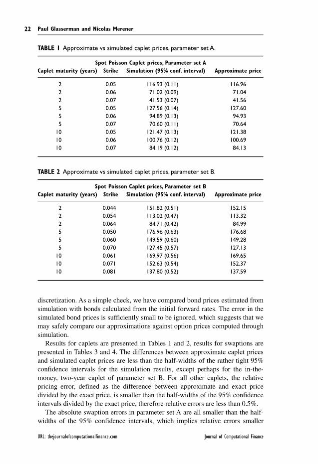
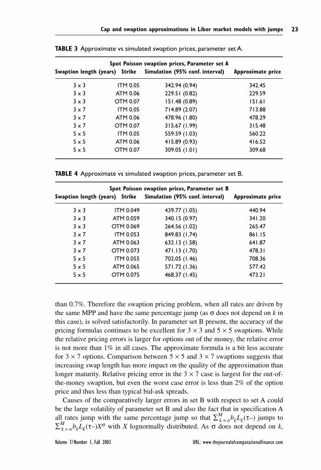
Results for caplets are presented in Tables 1 and 2, results for swaptions are presented in Tables 3 and 4. The differences between approximate caplet prices and simulated caplet prices are less than the half-widths of the rather tight 95% confidence intervals for the simulation results, except perhaps for the in-the-money, two-year caplet of parameter set B. For all other caplets, the relative pricing error, defined as the difference between approximate and exact price divided by the exact price, is smaller than the half-widths of the 95% confidence intervals divided by the exact price, therefore relative errors are less than 0.5%.
The absolute swaption errors in parameter set A are all smaller than the half-widths of the 95% confidence intervals, which implies relative errors smaller
TABLE 1 Approximate vs simulated caplet prices, parameter set A.
Spot Poisson Caplet prices, Parameter set ACaplet maturity (years) Strike Simulation (95% conf. interval) Approximate price
2 0.05 116.93 (0.11) 116.96 2 0.06 71.02 (0.09) 71.04 2 0.07 41.53 (0.07) 41.56 5 0.05 127.56 (0.14) 127.60 5 0.06 94.89 (0.13) 94.93 5 0.07 70.60 (0.11) 70.64 10 0.05 121.47 (0.13) 121.38 10 0.06 100.76 (0.12) 100.69 10 0.07 84.19 (0.12) 84.13
TABLE 2 Approximate vs simulated caplet prices, parameter set B.
Spot Poisson Caplet prices, Parameter set BCaplet maturity (years) Strike Simulation (95% conf. interval) Approximate price
2 0.044 151.82 (0.51) 152.15 2 0.054 113.02 (0.47) 113.32 2 0.064 84.71 (0.42) 84.99 5 0.050 176.96 (0.63) 176.68 5 0.060 149.59 (0.60) 149.28 5 0.070 127.45 (0.57) 127.13 10 0.061 169.97 (0.56) 169.65 10 0.071 152.63 (0.54) 152.37 10 0.081 137.80 (0.52) 137.59
Volume 7/Number 1, Fall 2003 URL: www.thejournalofcomputationalfinance.com
Cap and swaption approximations in Libor market models with jumps 23
than 0.7%. Therefore the swaption pricing problem, when all rates are driven by the same MPP and have the same percentage jump (as σ does not depend on k in this case), is solved satisfactorily. In parameter set B present, the accuracy of the pricing formulas continues to be excellent for 3 × 3 and 5 × 5 swaptions. While the relative pricing errors is larger for options out of the money, the relative error is not more than 1% in all cases. The approximate formula is a bit less accurate for 3 × 7 options. Comparison between 5 × 5 and 3 × 7 swaptions suggests that increasing swap length has more impact on the quality of the approximation than longer maturity. Relative pricing error in the 3 × 7 case is largest for the out-of-the-money swaption, but even the worst case error is less than 2% of the option price and thus less than typical bid-ask spreads.
Causes of the comparatively larger errors in set B with respect to set A could be the large volatility of parameter set B and also the fact that in specification A all rates jump with the same percentage jump so that ∑M
k = nbkLk(τ–) jumps to ∑M
k = nbkLk(τ–)Xσ with X lognormally distributed. As σ does not depend on k,
TABLE 3 Approximate vs simulated swaption prices, parameter set A.
Spot Poisson swaption prices, Parameter set ASwaption length (years) Strike Simulation (95% conf. interval) Approximate price
3 x 3 ITM 0.05 342.94 (0.94) 342.45 3 x 3 ATM 0.06 229.51 (0.82) 229.59 3 x 3 OTM 0.07 151.48 (0.89) 151.61 3 x 7 ITM 0.05 714.89 (2.07) 713.88 3 x 7 ATM 0.06 478.96 (1.80) 478.29 3 x 7 OTM 0.07 315.67 (1.99) 315.48 5 x 5 ITM 0.05 559.59 (1.03) 560.22 5 x 5 ATM 0.06 415.89 (0.93) 416.52 5 x 5 OTM 0.07 309.05 (1.01) 309.68
TABLE 4 Approximate vs simulated swaption prices, parameter set B.
Spot Poisson swaption prices, Parameter set BSwaption length (years) Strike Simulation (95% conf. interval) Approximate price
3 x 3 ITM 0.049 439.77 (1.05) 440.94 3 x 3 ATM 0.059 340.15 (0.97) 341.20 3 x 3 OTM 0.069 264.56 (1.02) 265.47 3 x 7 ITM 0.053 849.83 (1.74) 861.15 3 x 7 ATM 0.063 632.13 (1.58) 641.87 3 x 7 OTM 0.073 471.13 (1.70) 478.31 5 x 5 ITM 0.055 702.05 (1.46) 708.36 5 x 5 ATM 0.065 571.72 (1.36) 577.42 5 x 5 OTM 0.075 468.37 (1.45) 473.21
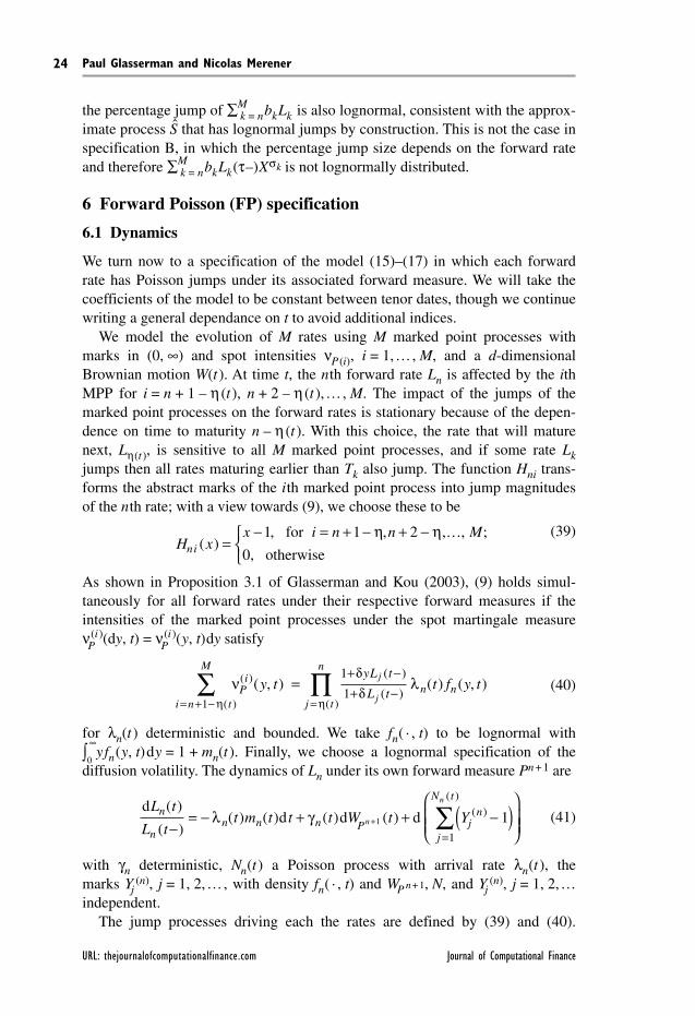
URL: thejournalofcomputationalfinance.com Journal of Computational Finance
Paul Glasserman and Nicolas Merener24
the percentage jump of ∑Mk = nbkLk is also lognormal, consistent with the approx-
imate process S that has lognormal jumps by construction. This is not the case in specification B, in which the percentage jump size depends on the forward rate and therefore ∑M
k = nbkLk(τ–)Xσk is not lognormally distributed.
6 Forward Poisson (FP) specification
6.1 Dynamics
We turn now to a specification of the model (15)–(17) in which each forward rate has Poisson jumps under its associated forward measure. We will take the coefficients of the model to be constant between tenor dates, though we continue writing a general dependance on t to avoid additional indices.
We model the evolution of M rates using M marked point processes with marks in (0, ∞) and spot intensities νP (i), i = 1,…, M, and a d-dimensional Brownian motion W(t ). At time t, the nth forward rate Ln is affected by the ith MPP for i = n + 1 – η (t ), n + 2 – η (t ),…, M. The impact of the jumps of the marked point processes on the forward rates is stationary because of the depen-dence on time to maturity n – η (t ). With this choice, the rate that will mature next, Lη(t ), is sensitive to all M marked point processes, and if some rate Lk jumps then all rates maturing earlier than Tk also jump. The function Hni trans-forms the abstract marks of the ith marked point process into jump magnitudes of the nth rate; with a view towards (9), we choose these to be
(39)H x
x i n n Mni ( )
, , , , ;
, =
− = + − + − …⎧⎨⎩
1 1 2
0
for
otherwise
η η
As shown in Proposition 3.1 of Glasserman and Kou (2003), (9) holds simul-taneously for all forward rates under their respective forward measures if the intensities of the marked point processes under the spot martingale measure νP
(i )(dy, t) = νP(i)(y, t)dy satisfy
(40)i n t
M
Pi
n nj t
n
y t t f y tyL t
L t
j
j= + − =∑ ∏=
+ −+ −
1
1
1η η
ν λδδ
( )
( )
( )
( , ) ( ) ( , )( )
( )
for λn(t ) deterministic and bounded. We take fn( · , t) to be lognormal with
∫0
∞yfn(y, t)dy = 1 + mn(t ). Finally, we choose a lognormal specification of the
diffusion volatility. The dynamics of Ln under its own forward measure Pn + 1 are
(41)d
d d dL t
L tt m t t t W t Yn
nn n n P j
n
j
N t
n
n( )
( )( ) ( ) ( ) ( ) ( )
( )
−= − + + −( )
⎛
⎝⎜⎜
⎞
⎠⎟⎟+
=∑λ γ 1 1
1
with γn deterministic, Nn(t ) a Poisson process with arrival rate λn(t ), the marks Yj
(n), j = 1, 2,…, with density fn( · , t) and WP n + 1, N, and Yj(n), j = 1, 2,…
independent.The jump processes driving each the rates are defined by (39) and (40).
Volume 7/Number 1, Fall 2003 URL: www.thejournalofcomputationalfinance.com
Cap and swaption approximations in Libor market models with jumps 25
Imposing these on the general model (15)–(17) leads to the dynamics of this specification under the spot martingale measure, given explicitly in Glasserman and Merener (2003). As discussed in Glasserman and Merener (2003), it is con-venient to visualize the process in the following way: under the spot martingale measure the rate closest to maturity Lη(t ) is driven by a jump process with total intensity
νδ
δλ
η
ηη ηP
i
i
Mt
tt ty t
y L t
L tt f y t( ) ( )
( )( ) ( )( , )
( )
( )( ) ( , )
=∑ =
++
1
1
1
and if Lη(t) + j jumps then Lη(t) + j + 1 jumps with probability
(42)ν
ν
δ
δ
λ
λη
η
η η
η η
Pi
i j
M
Pi
i j
M
t j
t j
t j t j
t j t j
y t
y t
y L t
L t
t f y t
t f y t
( )
( )
( )
( )
( ) ( )
( ) ( )
( , )
( , )
( )
( )
( ) ( , )
( ) ( , )
= +
= +
+ +
+ +
+ + + +
+ +
∑∑
=+
+2
1
1
1
1 11
1
Notice that, although different forward rates accept a given mark y with different state-dependent probabilities, all rates that jump, at a jump time, do it with the same mark y.
For the probabilities defined in (42) to be less than or equal than one, ie, for the intensities νP
(i) to be nonnegative, some restrictions apply on the parameters of the lognormal densities f and the functions λ(t). In particular,
(43)λ λj j k kt f y t t f y t j k( ) ( , ) ( ) ( , ) < >for
These restrictions are discussed in detail in Glasserman and Kou (2003) and Glasserman and Merener (2003). It suffices to state here that the numerical experiments in this paper are performed on parameter specifications that satisfy these restrictions.
6.2 Caplet pricing
The dynamics of each forward rate under its own forward measure is, by con-struction, of the form (9) with piecewise constant coefficients, as shown in Proposition 3.1 of Glasserman and Kou (2003). Therefore, in this specification, caplet prices are computed exactly through Proposition 3.1.
6.3 A swaption formula
In this section we develop a formula for the price of a swaption in the FP speci-fication. We will take advantage again of the powerful algorithm introduced in Proposition 3.1. To apply this, we need to identify a martingale process S of the form (9) that approximates, in a distribution sense, the dynamics of Sn, M under Pn, M. We will achieve this in two steps. First, we will introduce a process L that approximates the dynamics of the forward rates under Pn, M, as the exact dyna-mics of L under Pn, M are very complicated. Second, we will derive the dynamics
URL: thejournalofcomputationalfinance.com Journal of Computational Finance
Paul Glasserman and Nicolas Merener26
of S, based on the dynamics of L.For L we will a postulate a process in which each Lk (only k = n,…, M are
relevant to the swap) evolves exactly as Lk does under Pk + 1. In other words, we will approximate the dynamics of each forward rate under Pn, M with the dyna-mics under its own forward measure. This is clearly a crude approximation. A way to motivate this choice is as follows. We look at the change of intensity aris-ing when changing from the forward measure Pk + 1 (the one under which Lk has Poisson jumps) to the swap measure Pn, M. The Radon–Nikodym derivative that relates the measures is proportional to the ratio
M t
B t
B t
B tk n M
k
jj n
M
k
( )
( )
( )
( ), , ,
+
+=
+= = …
∑1
1
1
δ
If this ratio remains constant in time, then the intensities are unaffected by the change of measure because of Girsanov’s theorem (Theorem 3.12 in Björk, Kabanov, and Runggaldier, 1997). This is trivially true for n = M. But we also expect this ratio to remain approximately constant for n >> M – n + 1, because bonds in the numerator and denominator mature close to each other, and there-fore tend to fluctuate together. Intuitively, the dynamics of L should be a good approximation to the dynamics of L under Pn, M when M – n + 1, the swap length, is much smaller than the maturity date n.
In addition to specifying the marginal law of each Lk, we need to specify the dependence among their jumps. For this we devise a mechanism that approxi-mates the FP construction in (42). We specify a Poisson process Nn of jumps in Ln (the first rate relevant to the swap); each Lj, j = n + 1,…, M, then accepts or rejects a jump conditional on a jump in Lj – 1. More explicitly, we define
(44)d
d d dˆ ( )
ˆ ( )( ) ( ) ( ) ( ) ( )
( )L t
L tt m t t t W t Y
j
jj j j i
j
i
N tn
−= − + + −( )
⎛
⎝⎜⎜
⎞
⎠⎟⎟
=∑λ γ 1
1
with W a d-dimensional Brownian motion, Nn a Poisson process with rate λn(t ) , and Lj (0) = Lj (0). The mark Yi
(n) is lognormally distributed as fn( · , t) and, for j = n + 1,…, M,
(45)
if thenwith probability
otherwise
if then
, ,
,
,
( ) ( )( ) ( , )
( ) ( , )
( ) ( )
Y y Yy
Y Y
ij
ij
t f y t
t f y t
ij
ij
j j
j j−
−
= =⎧⎨⎪
⎩⎪
= =
− −1
1
1 1
1
1 1
λλ
This jump distribution is an approximation to the exact specification in (42). All rates evolve simultaneously under Pn, M with joint Poisson dynamics. Notice from (45) that the probability that Lj jumps with mark y given that Ln jumps with mark y is
Volume 7/Number 1, Fall 2003 URL: www.thejournalofcomputationalfinance.com
Cap and swaption approximations in Libor market models with jumps 27
(46)λ
λj j
n n
t f y t
t f y t
( ) ( , )
( ) ( , )
which is well-defined because of the restrictions on f and λ discussed at the beginning of this section. Since the jumps of Ln arrive with intensity λn(t ) fn(y, t) it follows that the effective jump process driving Lj has intensity λj(t ) fj (y, t). Therefore in this approximate process each rate evolves exactly as it would under its own forward measure. The dependence in the jumps of the Lj s approxi-mates the dependence in the jumps of the Lj s.
Our next goal is to approximate the dynamics of the swap rate under the Pn, M measure by a process S following
(47)d
d d dˆ( )
ˆ( )ˆ ( ) ˆ ( ) ˆ ( ) ( )
ˆ ( )S t
S tt m t t t W Yj
j
N t
= − + + −⎡
⎣
⎢⎢
⎤
⎦
⎥⎥=
∑λ γ 11
with γ (t ) deterministic, N(t ) a Poisson process with intensity λ(t ), Yj distributed as f ( · , t), lognormal with parameters µ(t ), σ(t ) and W, N, and Yj , j = 1, 2,… independent and S(0) = Sn, M(0). Fixing the weights bi (t ) in (5) at their time zero values bi we have
(48)S t b L tn M jj n
M
, ( ) ( )≈=∑
We apply Itô’s rule on the right side of (48) to motivate the choice of parameters in the dynamics of S. First, we look at the diffusion term
b L t t Wj j j Pj n
M
n M( ) ( ) ,γ d=∑
Matching this with the diffusion term in (47) we fix the forward rates at their ini-tial values Lj (0) and using the initial condition of S define
(49)ˆ ( )( )
( ) ( ),
γ γ γtS
b b L Ln M
j k j k j kk n
M
j n
M
≡⎡
⎣⎢⎢
⎤
⎦⎥⎥==
∑∑1
00 0
12
T
where the deterministic time dependence of the parameters γi (t) (through η(t)) is preserved.
Next, we focus on the jump term. The goal is to have a jump law in (47) that reproduces the total jump arrival rate and the conditional jump size probability of ∑M
j = nbj Lj (t ), which is our proxy for the swap rate.First, the total arrival rate. It follows from (45) that every jump time of Ln
is also a jump time of ∑Mj = nbj Lj (t ), and that there are no other jump times.
Therefore, the arrival rate of jump events is
URL: thejournalofcomputationalfinance.com Journal of Computational Finance
Paul Glasserman and Nicolas Merener28
(50)ˆ ( ) ( )λ λt tn≡
We continue with the jump magnitudes of S. We identify f lognormal that generates jump sizes approximately distributed as those of ∑M
j = nbj Lj (t ), by approximately matching moments of the jump magnitudes of S and ∑M
j = nbj Lj (t ). For the latter, conditional on the state of the system at a jump time τ we have
(51)
E
E
b L b L L
b L Y L
b L m
j j j jj n
M
j n
M
j jj
j n
M
j jj
nj
j n
M
ˆ ( ) ˆ ( ) , ˆ( )
ˆ ( ) , ˆ( )
ˆ ( )( )
( )( )
( )
τ τ τ τ
τ τ τ
τλ τλ τ
τ
− −⎡
⎣⎢⎢
⎤
⎦⎥⎥
= − − −[ ]
= −−−
−
==
=
=
∑∑
∑
∑
1
where we have used the conditional jump probability of Lj (46) and the fact that
∫0
∞(y – 1) fj (y, t)dy = mj (t). The expected jump size in (47), conditional on S at
the jump time s is
E Eˆ( ) ˆ( ) , ( ) ˆ( ) , ˆ( )
ˆ( ) ˆ
S s S s s S s S s Y s S s
S s m
j− − −[ ] = − − −[ ]= −
1
which suggests, by comparison with (51), fixing the rates at time zero an defin-ing m as
(52)ˆ ( )
ˆ ( ) ( )
ˆ ( )
( )
( )m t
b L m t
b L
j jt
t jj n
M
j jj n
M
j
n≡
=
=
∑∑
0
0
λλ
Next, we focus on matching the second moment of the jump magnitude con-ditional on being at a jump time. For ∑M
j = nbj Lj (t ) we have
(53)
E
E
b L b L L
b L Y L
b b L L
j j j jj n
M
j n
M
j jj
j n
M
i j i jj n
M
i
ˆ ( ) ˆ ( ) , ˆ( )
ˆ ( )( ) , ˆ( )
ˆ ( ) ˆ ( )
( )
τ τ τ τ
τ τ τ
τ τ
− −⎛⎝
⎞⎠ −⎡
⎣⎢⎤⎦⎥
= − −( )⎛⎝
⎞⎠ −⎡
⎣⎢⎤⎦⎥
= − −
==
=
=
∑∑
∑
∑
2
21
==∑ − − −[ ]
n
Mi jY Y LE ( )( ) , ˆ( )( ) ( )1 1 τ τ
Notice that (45) implies that if i < j then Y ( j ) ≠ 1 implies Y (i) = Y( j); in words, at a jump time, all rates maturing earlier than a jumping rate are also jumping rates, with the same mark. Therefore, denoting ξ ≡ max{i, j}
Volume 7/Number 1, Fall 2003 URL: www.thejournalofcomputationalfinance.com
Cap and swaption approximations in Libor market models with jumps 29
(54)
E E( )( ) , ˆ( ) ( ) , ˆ( )
( )
( )( ) ( , )
( )
( )( ) (
( ) ( ) ( )
( )
Y Y L Y L
t
ty f y y
t
tm m
i j
n
n
− − −[ ] = − −[ ]= − −
= + −( ) −
∞
−( )
∫
1 1 1
1
1 2
2
2
0
22
τ τ τ τ
λ
λτ
λ
λτ τ
ξ
ξξ
ξ σ τξ ξ
ξ
d
e −− −⎛⎝⎜
⎞⎠⎟
) 1
Using (54), we write (53) as
(55)b b L Lt
tm mi j i j
nj n
M
i n
Mˆ ( ) ˆ ( )
( )
( )( ) ( )
( )τ τ
λ
λτ τ
ξ σ τξ ξ
ξ− − + −( ) − − −⎛⎝⎜
⎞⎠⎟
==
−( )∑∑ e2
1 2 12
We match this with the expected squared jump size of S, at jump time s
ˆ( ) ( ) , ˆ( )
ˆ( ) ˆ ( ) ˆ ( )ˆ ( )
S s Y s S s
S s m s m s
j
s
− − −[ ]= − + −( ) − − −⎛
⎝⎞⎠
−( )
2 2
2 2
1
1 2 12
E
e σ
fix the rates at time zero, and use that S(0) = ∑Mj = nbj Lj (0) to enforce
e
e
ˆ ( ) ˆ ( ) ˆ ( )
ˆ ( ) ˆ ( )( )
( ) ( ) ( )
ˆ ( ) ˆ (
( )
σ
λλ
ξ σξξ ξ
2
1 2 12
0 0 1 2 1
0
2 2
t m t m t
b b L Lt
t m t m t
b b L L
i j i j n
t
i j i j
j n
M
i n
M
( )
⎛⎝
⎞⎠
⎛
⎝⎜
⎞
⎠⎟
+( ) − −
=
⎛⎝
⎞⎠
== + − −∑∑00)
j n
M
i n
M
== ∑∑
Finally, using that m(t ) = e(µ (t ) + (σ (t ))2) ⁄ 2) – 1 we get
(56)
ˆ ( ) logˆ ( ) ˆ ( ) ( ) ( )
ˆ ( ) ˆ ( ) ˆ ( )
( )
( )( )
σ
λ
λξ σξ
ξ ξt
b b L L m t m t
m t b b L L
i j i j
i j i j
t
tn
t
j n
M
i n
M
j n
M
i n
M
20 0 1 2 1
1 0 0
2 2
2=⎛ ( )
==
==
+ − −
+
⎛⎝
⎞⎠
⎛⎝⎜
⎞⎠⎟
( )∑∑
∑∑
e
⎝⎝⎜⎜
+⎞
⎠⎟⎟
++( )1 2
1 2
ˆ
ˆ ( )
m
m t
and
(57)ˆ ( ) log ˆ ( )ˆ ( )µ σ
t m tt= +( ) −12
2
where m is given by (52). The evolution of S is given then by (47) with (49), (50), (56) and (57). The swaption price is then computed using Proposition 3.1 on the rate S.
URL: thejournalofcomputationalfinance.com Journal of Computational Finance
Paul Glasserman and Nicolas Merener30
6.4 Numerical results
We investigate now the accuracy of the swaption formula introduced in the previous section. Results are then compared to swaption prices obtained using (6), where the expected discounted payoff is computed via Monte Carlo simula-tion of the term structure under the spot martingale measure. We generate the sample paths of the term structure using a first order discretization scheme on the logarithm of the forward rates as implemented and discussed in Glasserman and Merener (2003). With the accrual period fixed at δ = 0.5, taking the time step to be less than 0.1 ensures (empirically) that the bias in the simulated price is less that 0.1% of the exact price. Simulated swaption prices are then very good approximation to the exact price and provide a benchmark for testing the approximate method of Section 6.3.
For simplicity, we perform numerical tests driven by a one factor diffusion and M marked point processes, although the method can handle multidimensional diffusions. The parameters are held constant between tenor dates. Moreover, we make the model stationary in the sense that the parameters of the k th rate depend on the number of accrual periods to maturity, k – η(t). As before, γk (Tj) denotes the diffusive volatility of Lk during the accrual period ending at Tj. A consequence of this stationary specification is that all rates follow, under their respective forward measures and for a fixed distance to their own maturities, the same stochastic differential equation. The initial term structure is increasing, Lk(0) = log(1.051271 + 0.0011178 × k) and the accrual period is δ = 0.5. The choice of parameters we present next are close to those of model specification SP but not identical as we need to satisfy restriction (43). The parameters are as follows.
Parameter Set A: For all j, k,
γ
λ σ µ
k j
k jk j
k jk j
k j
T
T T T
( ) . ,
( ) . , ( ) . . , ( ) .
=
= × = × =− −
0 1
5 0 9 0 1 0 95 0 0
The total instantaneous volatility of the rate next to mature (k = j) is approxi-mately 0.245, the diffusion square volatility is 0.01 and the jump squared volatility is 0.06 so most of the volatility of the maturing rate is due to jumps. The jump volatility decreases as rates are more distant from maturity.
Parameter Set B: For all j, k,
γ
λ σ µ
k j
k jk j
k jk j
k j
T
T T T
( ) . ,
( ) . , ( ) . . , ( ) .
=
= × = × = −− −
0 1
5 0 9 0 2 0 9 0 1
The total instantaneous volatility of the rate next to mature is approximately 0.46, the diffusion square volatility is 0.01 and the jump square volatility is 0.2, therefore almost all the volatility of the rate next to mature is due to jumps. As in parameter set A, jump volatility decreases as rates are more distant from maturity.
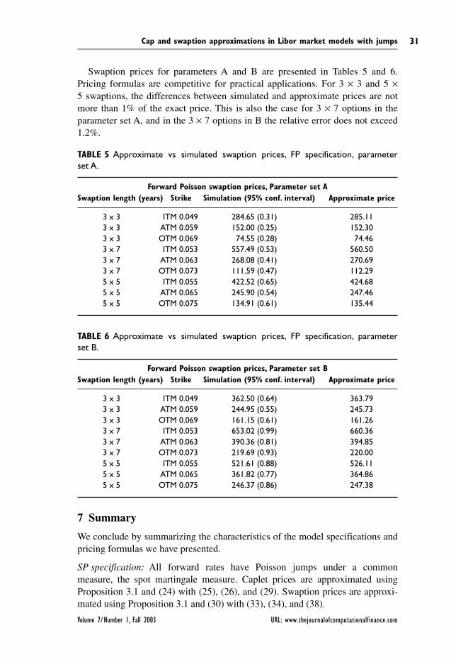
Volume 7/Number 1, Fall 2003 URL: www.thejournalofcomputationalfinance.com
Cap and swaption approximations in Libor market models with jumps 31
Swaption prices for parameters A and B are presented in Tables 5 and 6. Pricing formulas are competitive for practical applications. For 3 × 3 and 5 × 5 swaptions, the differences between simulated and approximate prices are not more than 1% of the exact price. This is also the case for 3 × 7 options in the parameter set A, and in the 3 × 7 options in B the relative error does not exceed 1.2%.
TABLE 6 Approximate vs simulated swaption prices, FP specification, parameter set B.
Forward Poisson swaption prices, Parameter set BSwaption length (years) Strike Simulation (95% conf. interval) Approximate price
3 x 3 ITM 0.049 362.50 (0.64) 363.79 3 x 3 ATM 0.059 244.95 (0.55) 245.73 3 x 3 OTM 0.069 161.15 (0.61) 161.26 3 x 7 ITM 0.053 653.02 (0.99) 660.36 3 x 7 ATM 0.063 390.36 (0.81) 394.85 3 x 7 OTM 0.073 219.69 (0.93) 220.00 5 x 5 ITM 0.055 521.61 (0.88) 526.11 5 x 5 ATM 0.065 361.82 (0.77) 364.86 5 x 5 OTM 0.075 246.37 (0.86) 247.38
TABLE 5 Approximate vs simulated swaption prices, FP specification, parameter set A.
Forward Poisson swaption prices, Parameter set ASwaption length (years) Strike Simulation (95% conf. interval) Approximate price
3 x 3 ITM 0.049 284.65 (0.31) 285.11 3 x 3 ATM 0.059 152.00 (0.25) 152.30 3 x 3 OTM 0.069 74.55 (0.28) 74.46 3 x 7 ITM 0.053 557.49 (0.53) 560.50 3 x 7 ATM 0.063 268.08 (0.41) 270.69 3 x 7 OTM 0.073 111.59 (0.47) 112.29 5 x 5 ITM 0.055 422.52 (0.65) 424.68 5 x 5 ATM 0.065 245.90 (0.54) 247.46 5 x 5 OTM 0.075 134.91 (0.61) 135.44
7 Summary
We conclude by summarizing the characteristics of the model specifications and pricing formulas we have presented.
SP specification: All forward rates have Poisson jumps under a common mea sure, the spot martingale measure. Caplet prices are approximated using Proposition 3.1 and (24) with (25), (26), and (29). Swaption prices are approxi-mated using Proposition 3.1 and (30) with (33), (34), and (38).
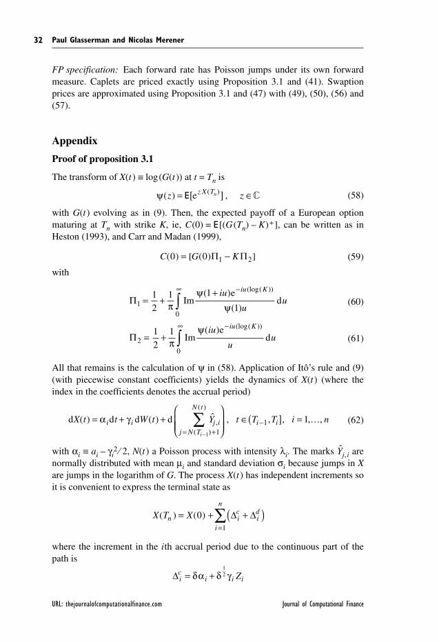
URL: thejournalofcomputationalfinance.com Journal of Computational Finance
Paul Glasserman and Nicolas Merener32
FP specification: Each forward rate has Poisson jumps under its own forward measure. Caplets are priced exactly using Proposition 3.1 and (41). Swaption prices are approximated using Proposition 3.1 and (47) with (49), (50), (56) and (57).
Appendix
Proof of proposition 3.1
The transform of X(t ) ≡ log(G(t )) at t = Tn is
(58)ψ( ) , ( )z zz X Tn= [ ] ∈E e �
with G(t ) evolving as in (9). Then, the expected payoff of a European option maturing at Tn with strike K, ie, C(0) = E [(G (Tn) – K) + ], can be written as in Heston (1993), and Carr and Madan (1999),
(59)C G K( ) ( )0 0 1 2= −[ ]Π Π
with
(60)
(61)
Π
Π
1
0
2
0
1
2
1 1
1
1
2
1
= ++
= +
−∞
−∞
∫
∫
πψ
ψ
πψ
Im( )
( )
Im( )
(log( ))
(log( ))
iu
uu
iu
uu
iu K
iu K
ed
ed
All that remains is the calculation of ψ in (58). Application of Itô’s rule and (9) (with piecewise constant coefficients) yields the dynamics of X(t ) (where the index in the coefficients denotes the accrual period)
(62)d d d dX t t W t Y t T T i ni i j ij N T
N t
i i
i
( ) ( ) ˆ , , , , ,,( )
( )
= + +⎛
⎝⎜⎜
⎞
⎠⎟⎟
∈( ] = …= +
−−
∑α γ1 1
1 1
with αi ≡ ai – γi2 ⁄ 2, N(t ) a Poisson process with intensity λi. The marks Yj, i are
normally distributed with mean µi and standard deviation σi because jumps in X are jumps in the logarithm of G. The process X(t ) has independent increments so it is convenient to express the terminal state as
X T Xn ic
id
i
n
( ) ( )= + +( )=∑0
1
∆ ∆
where the increment in the ith accrual period due to the continuous part of the path is
∆ ic
i i iZ= +δα δ γ12
Volume 7/Number 1, Fall 2003 URL: www.thejournalofcomputationalfinance.com
Cap and swaption approximations in Libor market models with jumps 33
with {Z1, Z2,…, Zn} independent and standard normally distributed. The incre-ment in the ith accrual period due to the jumps is the sum of the magnitudes of the jumps occurring in (Ti – 1, Ti]
∆ id
j iYj N T
N T
i
i
= ˆ,
( )
( )
= +−
∑1 1
and the total number of jumps in (Ti – 1, Ti], denoted by Ni, is a Poisson random variable with parameter δ λi. Since the {∆i
d, ∆id} are mutually independent we
have from (58)
ψ( ) ( )z z X z z
i
nic
id
= [ ] [ ]=
∏e e e0
1
E E∆ ∆
The transform of a Poisson number of normally distributed jumps is easily cal-culated and is given explicitly in Scott (1997):
E e ezi
z zid
i i∆[ ] = −( )[ ]+( )exp δλ µ σ2 2 2 1
Because ∆ci is normally distributed we write
E e ez z zic
i i∆[ ] = +( )[ ]δ α γ2 2 2
Therefore,
(63)ψ δλ δα δγµ σ( ) exp ( )z zX z ziz z
i ii
ni i= + −⎛
⎝⎞⎠ + +
⎡
⎣⎢⎢
⎤
⎦⎥⎥
+( )
=∑0 1 2
2 2 2 2 2
1
e
Next, we insert (63) with z = 1 + iu, and (63) with z = 1, in (60), and insert (63) with z = iu in (61), and work tedious but straightforward algebra to obtain (11)–(12). The time-zero European option price is given by [G(0)Π1 – KΠ2].
Proof of Lemma 4.1
Proof of Lemma 4.1 is a special case of the proof of Lemma 4.2 as the numeraire associated with Pn + 1 is proportional to the numeraire associated with Pn, n
Proof of Lemma 4.2
First, some notation. An MPP can be described through a random measure µ(dx, dt) on the product of the mark space and the time axis assigning unit mass to each point (τj, Xj). This representation makes it possible to write ∑j
N=(t )1H (Xj , τj) = ∫0
t∫�DH(x, s)µ(dx, ds).
Now the proof. We want to identify the change in intensity associated with changing from the spot measure P to the swap measure Pn, M. Define

URL: thejournalofcomputationalfinance.com Journal of Computational Finance
Paul Glasserman and Nicolas Merener34
Z tM t
B t( )
( )
( )=
with M(t ) as in (7). Because M is a linear combination of asset prices, Z is a martingale under the spot measure. From (1) and (7) it follows that
Z tL T L tj j k n
M
jj t
k
j
t
( )( ) ( )
( )
( )
=+ += ==
−
∑ ∏∏ 1
1
1
10
1
δδ
δη
η
Itô’s formula and the dynamics of L (15)–(17) give the dynamics of Z. At τ, a jump time of the ith MPP, with mark X, the percentage jump in Z is
Z Z
Z
L H X
L
k n
M
j jij t
k
k n
M
jj t
k
( ) ( )
( )
( )( ( , ))
( )
( )
( )
τ ττ
δδ τ τ
δδ τ
η
η
− −−
=+ − +
+ −
−= =
= =
∑ ∏∑ ∏
11 1
11
1
which can be written as
δδ τ
δ τδ τ τ
δδ τ
η η
η
k n
M
jj t
k j
j j ij t
k
k n
M
jj t
k
L
L
L H X
L
= = =
= =
∑ ∏ ∏∑ ∏+ −
+ −+ − +
+ −
−
11
1
1 11
1
1( )
( )
( )( ( , ))
( )
( ) ( )
( )
Multiplying numerator and denominator by Bη(t ) and recalling the definition of the weight bk in (5) this expression simplifies to
bL
L H Xkk n
Mj
j j ij t
k
= =∑ ∏ + −
+ − +−
1
1 11
δ τδ τ τη
( )
( )( ( , ))( )
Now we aggregate the (non-simultaneous) jumps from the r MPPs driving L, and write the dynamics of Z in the random measure notation, where the drift follows from the martingale condition
(64)
dd
d d d d
Z t
Z tW b
L t
L t H x t
x t x t t
P kk n
Mj
j j ij t
k
i
r
Pi
Pi
D
( )
( )
( )
( )( ( , ))
( , ) ( , )
( )
( ) ( )
−= … +
+ −+ − +
−⎛
⎝⎜⎜
⎞
⎠⎟⎟
× −( )= ==∑ ∏∫∑ 1
1 11
1
δδ
µ ν
η�
Next we define the swap measure Pn, M through the Radon–Nikodym derivative
d
d
P
PZ t
B
M
n M
t
,
( )( )
( )
⎛
⎝⎜⎞
⎠⎟= 0
0
Volume 7/Number 1, Fall 2003 URL: www.thejournalofcomputationalfinance.com
Cap and swaption approximations in Libor market models with jumps 35
and invoke Girsanov’s theorem (in the form in Theorem 3.12 in Björk, Kabanov, and Runggaldier, 1997) to identify the change in intensity associated to the change of measure. Girsanov’s theorem states that given a P-martingale process A(t ), (P not necessarily being the spot measure) with
d ( )
( )d d d d d
A t
A tW x t x t x tP
P PD
−= + − −[ ]∫Γ Φ( ( , ) ) ( , ) ( , )1 µ ν
�
and under technical conditions, there is an equivalent measure Q with Radon–Nikodym derivative
d
d
Q
PA t
t
⎛⎝⎜
⎞⎠⎟
= ( )
such that dWP = Γdt + dWQ with WQ a Brownian motion under Q, and the intensity of the driving jump process under Q is νQ(dx, t) = Φ(x, t)νP(dx, t). As we have r MPPs, we invoke Lemma A.1 in Appendix A of Glasserman and Kou (2003) which uses Girsanov’s theorem to get the intensity of each MPP,
νδ
δν
ηP
ik
k n
Mj
j j ij t
k
Pi
n M x t b tL t
L t H x tx t,
( )
( )
( )( , ) ( )( )
( )( ( , ) )( , )d d=
++ +
⎛
⎝⎜⎜
⎞
⎠⎟⎟
= =∑ ∏ 1
1 1
with bk(t ) = Bk + 1(t ) ⁄M(t ).
REFERENCES
Andersen, L., and Andreasen, J. (2000). Volatility skews and extensions of the Libor market model. Applied Mathematical Finance 7, 1–32.
Björk, T., Kabanov, Y., and Runggaldier, W. (1997). Bond market structure in the presence of marked point processes. Mathematical Finance 7, 211–39.
Black, F. (1976). The pricing of commodity contracts. Journal of Financial Economics 3, 167–79.
Brace, A., Dun, T., and Barton, G. (2001). Towards a central interest rate model. In Handbooks in Mathematical Finance. Topics in Option Pricing, Interest Rates and Risk Management. Cambridge University Press.
Brace, A., Gatarek, D., and Musiela, M. (1997). The market model of interest rate dynamics. Mathematical Finance 7, 127–55.
Brémaud, P. (1981). Point Processes and Queues: Martingale Dynamics. Springer, New York.
Carr, P., and Madan, D. (1999). Option valuation using the fast Fourier transform. Journal of Computational Finance 2 (Summer), 61–74.
Duffie, D., Pan, J., Singleton, K. (2000). Transform analysis and asset pricing for affine jump-diffusions. Econometrica 68, 1343–76.
Glasserman, P., and Kou, S. G. (2003). The term structure of simple forward rates with jump risk. Mathematical Finance, July, 383–410.
URL: thejournalofcomputationalfinance.com Journal of Computational Finance
Paul Glasserman and Nicolas Merener36
Glasserman, P., and Merener, N. (2003). Numerical solution of jump-diffusion LIBOR market models. Forthcoming in Finance and Stochastics 7, 1–27.
Heston, S. L. (1993). A closed-form solution for options with stochastic volatility with appli-cations to bond and currency options. The Review of Financial Studies 6, 327–43.
Hull, J., and White, A. (2000). Forward rate volatilities, swap rate volatilities and the imple-mentation of the LIBOR market model. Journal of Fixed Income 10 (September), 46–62.
Jäckel, P., and Rebonato, R. (2000). Linking caplet and swaption volatilities in a BGM/J framework: Approximate solutions. Working paper, QUARC, Royal Bank of Scotland, London. Available at www.rebonato.com.
Jamshidian, F. (1997). LIBOR and swap market models and measures. Finance and Stochastics 1, 293–330.
Jamshidian, F. (1999). LIBOR Market model with semimartingales. Working paper, NetAnalytic Ltd., London.
Joshi, M., and Rebonato, R. (2001). A stochastic-volatility, displaced-diffusion extension of the LIBOR market model. Working paper, QUARC, Royal Bank of Scotland, London. Available at www.rebonato.com.
Kawai, A. (2000). Swaption pricing in the LIBOR market model. Working paper, School of Mathematics, University of New South Wales.
Kloeden, P. E., and Platen, E. (1992). Numerical Solution of Stochastic Differential Equations. Springer-Verlag, Berlin.
Kou, S. G. (1999). A jump diffusion model for option pricing with three properties: leptokur-tic feature, volatility smile, and analytical tractability. Working paper, Columbia University, Available at www.ieor.columbia.edu/~kou.
Merton, R. (1976). Option pricing when underlying stock returns are discontinuous. Journal of Financial Economics 3, 125–44.
Mikulevicius, R., and Platen, E. (1988). Time discrete Taylor approximations for Ito processes with jump component. Mathematische Nachrichten 138, 93–104.
Miltersen, K. R., Sandmann, K, and Sondermann, D. (1997). Closed-form solutions for term structure derivatives with lognormal interest rates. Journal of Finance 52, 409–30.
Musiela, M., and Rutkowski, M., Martingale (1997). Methods in Financial Modeling. Springer, New York.
Scott, L. O. (1997). Pricing stock options in a jump-diffusion model with stochastic volatil-ity and interest rates: application of Fourier inversion methods. Mathematical Finance 7, 413–26.
Zühlsdorff, C. (2000). Extended Libor market models with affine and quadratic volatility. Discussion paper, Department of Statistics, University of Bonn Available at www.finasto. unibonn.de.