J. Appl. Environ. Biol. Sci., 6(9)123-138, 2016

© 2016, TextRoad Publication

ISSN: 2090-4274

Journal of Applied Environmental

and Biological Sciences www.textroad.com

*Corresponding Author: Hussein Abdullatif Dghayes, College of Engineering Technology, Janzour, Tripoli, Libya

Dgheyes@yahoo.com

The Power System Stability Boundary for Two-Finite

Machine System

Hussein Abdullatif Dghayes

College of Engineering Technology, Janzour Tripoli, Libya

Received: July 22, 2016

Accepted: October 6, 2016

ABSTRACT

Analysis of the stability boundary of power system following a transient disturbance, which distinguish reliably

between stable and unstable system that involves the study of large set of non-linear differential equations solved

using some computer techniques are based on a two-finite machine, interconnected by passive loads, power system

model in which the classical representation is used for each machine and resistance is neglected. There are two

different method used in to determine the stability boundary of power system. The first method is the equal-area

criterion and second is the phase plane technique, both are compared and the final approaches giving identical results

for the simplified model.

1.1 INTRODNCTION

A typical modern power system consists of a large number of generating plants and loads, interconncted

through a complex network of transmission and distribution lines.To maintain synchronism between the vaious parts

of a power system becomes increasingly diffecult on inteconnection between system continue to grow. The

dependence of the modern society on electrical energy requires that major power failure be avoided . The loss of

synchronism between generators and concentrated loads, caused by power failures or system faults, presents a

potential cause of power failures. In order to evaluate the hazards and to take steps to prevent loss of synchronism,

accurate methods of analysis of on-line system stability must be developed and put into use. Current practice usually

involves analytical studies which result in system design or operating procedure modifications. Even with the use of

modern digital computer modeling, this approach does not fully protect the modern large scale system during

emergency fault conditions.

This paper considers the simulation of a proven system, which is modeled by a two-machine equivalent system,

during possible fault and erratic operating conditions. A goal is to seek, by analytical investigation, the range of

operating limitations for continual safe and reliable operation of such a power system. The basic approach used

involves a computer stability simulation of the composite generator and equivalent loads.

The first approach to the problem which gives conservative results is used. This is an extension of the standard

procedure used in transient stability studies known as the step-by-step method. The problem may be formulated as

follows: given a system initially in a steady operation and assume a disturbance at time t� . Then the question: is

there a stable equilibrium position for the system after the disturbance is cleared , and if so, what the critical clearing

time, that is, the maximum time that the per- disturbances may remain, before the system loses its capability to return

to steady-state .

1.2 POWER SYSTEMSTABILITY

Stability studies will be divided into three different categories depending on the extent of the disturbance on

the system. Steady-state- stability, infinitely small disturbances, small angle changes, time invariant (��� =0),

manual control of voltage no automatic voltage regulator. Dynamic stability, smaller or normal random impacts ,

system equations are linear (or have been linearized) about an operating point , X� =AX+Bu, eigenvalues of A matrix

may be time-varying and that u may be used to present several inputs including system load responses, automatic

control devices and voltage regulator action (Δ��� ≠0), multiple swing (Decay of Oscillations). Transient stability,

nonlinear, first Swing cycle is most important, caused by large disturbances, X� =f(x, u ,t ), time solutions, use digital

computer .

123

Dghayes, 2016

1.3 METHODS OF SIMULATION

The first step in a stability study is to make a mathematical model of the system during the fault. The

elements included in the model are those affecting the dynamics of the machines (acceleration or deceleration of the

machine rotors). Generally, the elements of the power system that influence the electrical and mechanical torques of

the machines should be included in the model. These elements are: The network before, during, and after disturbance

. The parameters of the synchronous machines .The loads and their characteristics. The excitation systems .The

mechanical turbines and speed governors. System components such as transformers and capacitors.

The complexity of the model depends upon the type of transient and system being investigated in the study. Using the

techniques of modern control theory, the system stability of a large nonlinear system can be determined without

obtaining the solution of the differential equations. That is, the stability limit can be calculated directly from the

system equations and used during system operation.

In this papersthe close relationship of two different methods of analyzing stability boundary will be discussed. These

are the classical equal-area criterion, the phase plane trajectories technique. These will be demonstrated for the case

of two connected finite machines.

1.4CLASSICAL MODEL

Transient stability studies are performed to determine if system will remain in synchronism subsequent to the

occurrences a major disturbance. That is, will the machine rotors remain in synchronism and will they return to a

constant speed of operation following the disturbance. Classical stability study assumption are : (1) mechanical power

input held constant,(2)damping is neglected, (3)loads are represented by passive impedance,(4)each machine has a

constant-voltage behind transient reactance, (5)the mechanical rotor angle of each machine coincides with the angle

of the voltage behind transient reactance,(6)machine saturation is neglected.

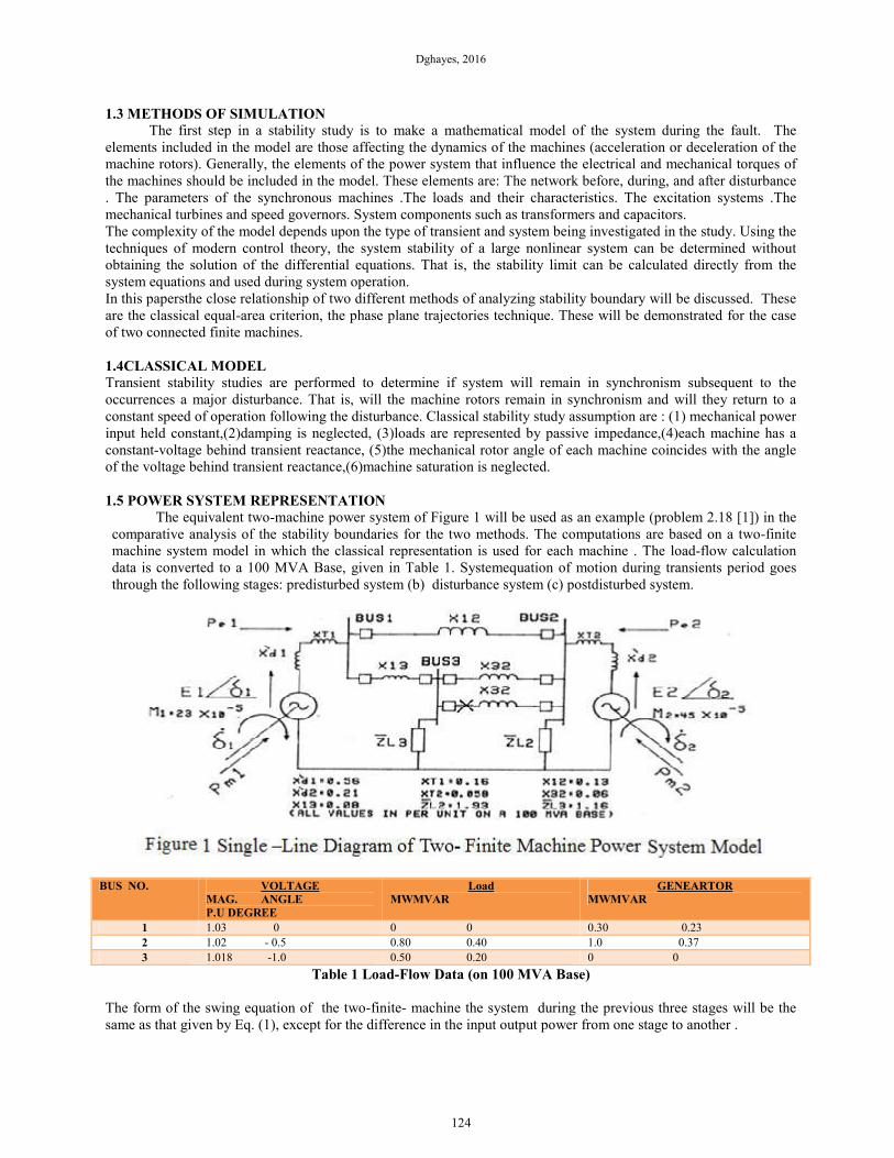
1.5 POWER SYSTEM REPRESENTATION

The equivalent two-machine power system of Figure 1 will be used as an example (problem 2.18 [1]) in the

comparative analysis of the stability boundaries for the two methods. The computations are based on a two-finite

machine system model in which the classical representation is used for each machine . The load-flow calculation

data is converted to a 100 MVA Base, given in Table 1. Systemequation of motion during transients period goes

through the following stages: predisturbed system (b) disturbance system (c) postdisturbed system.

BUS NO. VOLTAGE

MAG. ANGLE

P.U DEGREE

Load

MWMVAR

GENEARTOR

MWMVAR

1 1.03 0 0 0 0.30 0.23

2 1.02 - 0.5 0.80 0.40 1.0 0.37

3 1.018 -1.0 0.50 0.20 0 0

Table 1 Load-Flow Data (on 100 MVA Base)

The form of the swing equation of the two-finite- machine the system during the previous three stages will be the

same as that given by Eq. (1), except for the difference in the input output power from one stage to another .

124

J. Appl. Environ. Biol. Sci., 6(9)123-138, 2016

( )12 12 12(1)a m eP P P M

..δ = = −

The equation of electrical power output from a machine is given by

2n

ei i ii i j ij ij i ji=1

e1 1 2

e2 2 1

2 e1 1 e2e12

1 2

j i

P 0.094 1.16 (77.4 )

P 0.698 1.16 (77.4 )

M P M PSince P

M M

P E G E E Y cos (2)

cos (3)

cos (4)

(5)

( )θ δ δ

δ δ

δ δ

≠= + °

= + °

−=

+

= + −

−

−

+∑

++

2 21 2

5 5M M

e12 12

23Where 10 sec ./ele deg. 45 10 sec ./ele deg.

Then P 0.177 1.135 ( 4.1 )

,

sin (6)δ

− −= × = ×

= − + + °

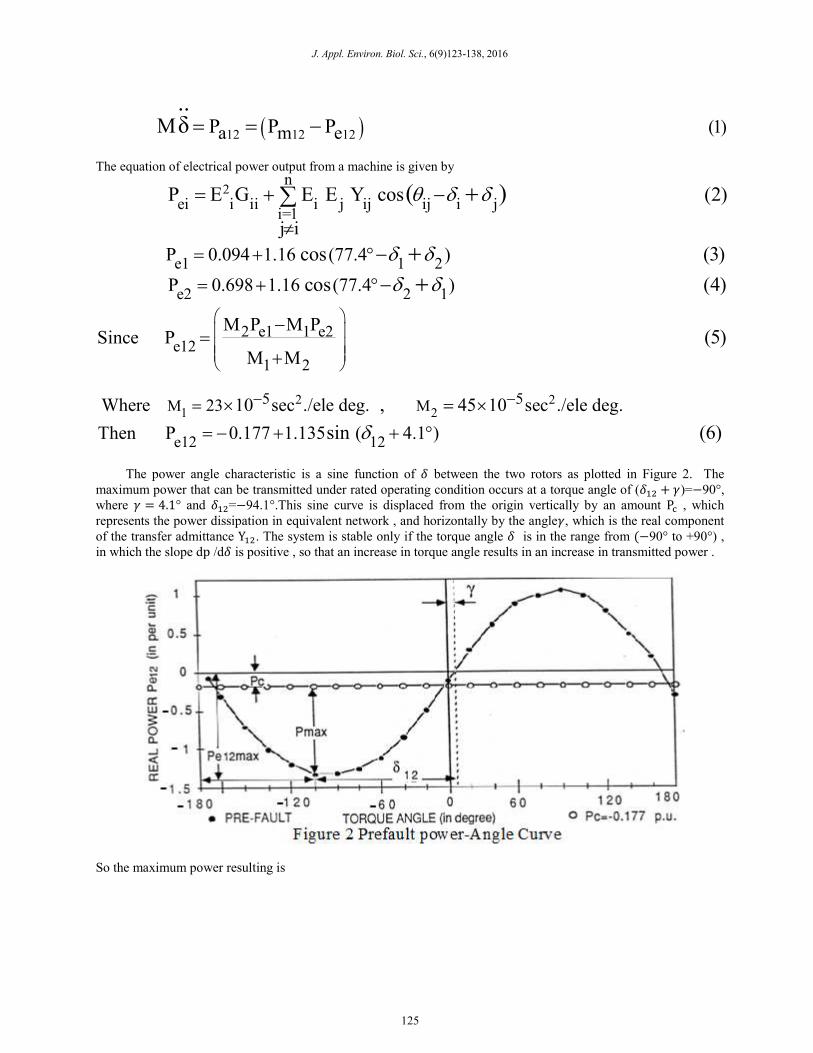
The power angle characteristic is a sine function of between the two rotors as plotted in Figure 2. The

maximum power that can be transmitted under rated operating condition occurs at a torque angle of (�� + �)=−90°,

where � = 4.1° and ��=−94.1°.This sine curve is displaced from the origin vertically by an amount P� , which

represents the power dissipation in equivalent network , and horizontally by the angle�, which is the real component

of the transfer admittance Y��. The system is stable only if the torque angle is in the range from (−90° to +90°) ,

in which the slope dp /d is positive , so that an increase in torque angle results in an increase in transmitted power .

So the maximum power resulting is

125

Dghayes, 2016

12 12

e12max

e12max 12

m e

2 m1 1 m2m12

1 2

P 0.177 1.135 ( 94.1 )

P 1.31 P.u occurs at ( 94.1 ) or ( 1.642 rad.)

And the steady state synchronous speed , P =P , is

M P M PP 0.1452 P.u

M M

0.1452 0.17

sin (7)

(8)

δ

= − + − °

= − = − ° −

−= = −

+

− = −

0 0

07 1.135 ( 4.1 )

arcsin( 4.1 ) 0.0318 2.5 (0.0436 rad.)

sin δδ δ

+ + °

+ ° = = − °⇒

The disturbance to be considered is permanent three-phase fault which occurs near bus number 3 at the end of line 5.

The power angle characteristic for disturbed and postdisturbed system are sin wave having smaller amplitudes than that for the predisturbed system.

12

12

12

e12

e12

e12

Predisturbed system P 0.177 1.135 ( 4.1 )

Disturbed system P 0.0026 0.061 ( 1.0 )

Postdisturbed system P 0.1670 1.120 ( 4.3 )

sin

sin

sin

δ

δ

δ

= − + + °

= − + + °

= − + + °

The steady-state values of Pe��, and (d�δ/d�t) for the stable post disturbance system are:

m12 e12P P 0.1452 P.u

0.1452 0.167 1.12 ( 4.3 )ss

(seady state)

sin δ

= = −

− = − + + °

( )

2

2

d ssarcsin ( 4.3 ) 0.0218 3.2 ( 0.0558 rad.) and 0ss ssdt

From the power -angle digram shown in Figure 5 . max. ss

176.8 ( 3.0857 rad. )max.

δδ δ

δ π δδ

+ ° = = − ° − =

= − ° −

⇒ ⇒

= − −

The analysis of first-swing classical transient stability constitute the important tools for judging system performance. The reason for its relative importance is that if the system is stable on first swing, it will for most cases be stable on

the subsequent swings. The torque angle is calculated as a function of time over a period long enough determine

whether will to increase without limit or reach a maximum and start to decrease.

Numerical methods for solution of differential equations, the methods most commonly used for the solution of the differential equations are: Euler method, the modified-Euler method, Runge-Kutta and the trapezoidal method. Each

of these has advantages and disadvantages which are associated with numerical stability, time-step size,

computational effort per integration step and accuracy of the obtained solutions.

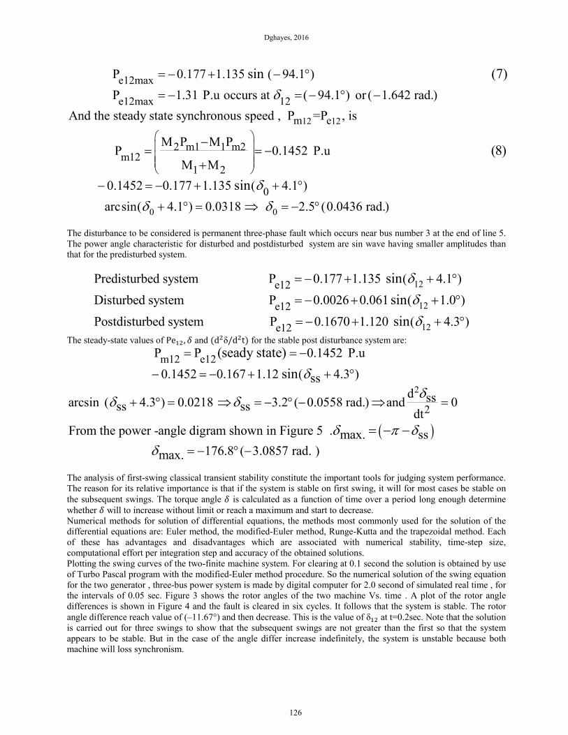
Plotting the swing curves of the two-finite machine system. For clearing at 0.1 second the solution is obtained by use

of Turbo Pascal program with the modified-Euler method procedure. So the numerical solution of the swing equation

for the two generator , three-bus power system is made by digital computer for 2.0 second of simulated real time , for the intervals of 0.05 sec. Figure 3 shows the rotor angles of the two machine Vs. time . A plot of the rotor angle

differences is shown in Figure 4 and the fault is cleared in six cycles. It follows that the system is stable. The rotor

angle difference reach value of (–11.67°) and then decrease. This is the value of δ�� at t=0.2sec. Note that the solution

is carried out for three swings to show that the subsequent swings are not greater than the first so that the system

appears to be stable. But in the case of the angle differ increase indefinitely, the system is unstable because both machine will loss synchronism.

126

J. Appl. Environ. Biol. Sci., 6(9)123-138, 2016

1.6STABILITY DOMAIN

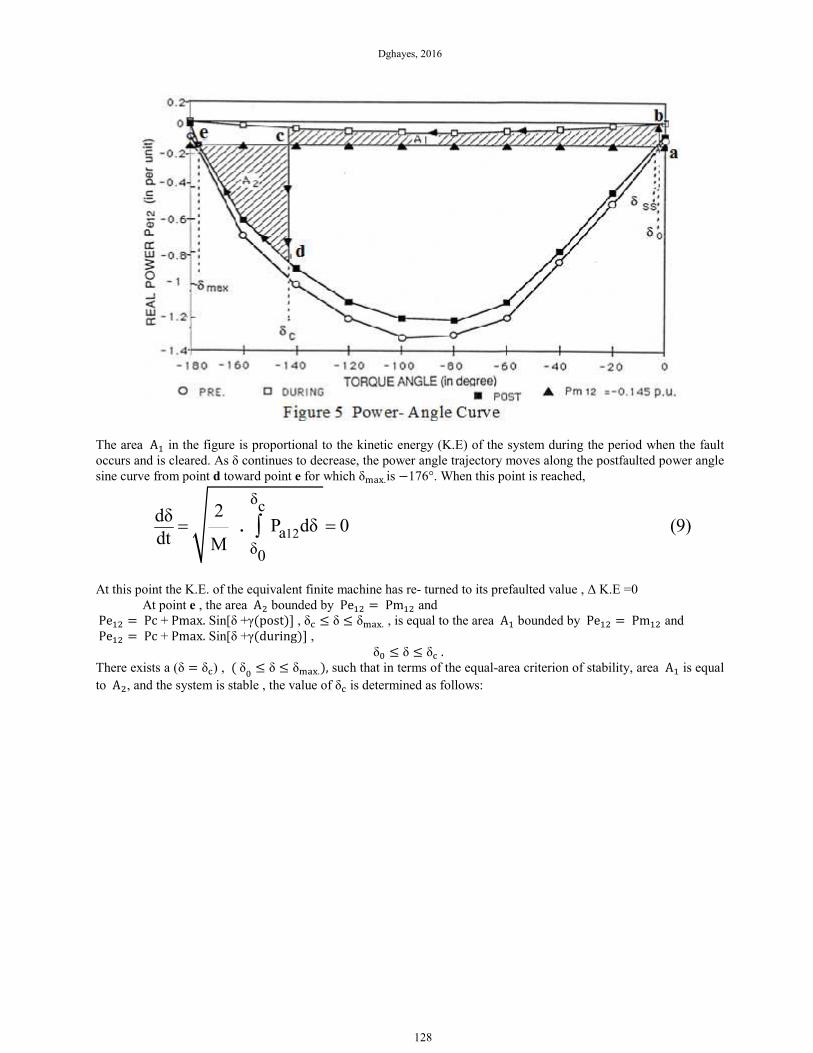
To study the stability domain of a power system during a fault, the first method is power-angle characteristics

and the equal-area criterion are shown in Figure 5 , for condition before, during, and after a three phase fault . The

horizontal line denoted by P= Pm�� represents the equivalent mechanical power input to machine. Before occurrence

of the fault , the two the machine were operating at synchronous speed with a rotor angle at t=0 is δ� = −2.5 degree

as indicated by the intersection of Pm�� with the prefault curve, this operating point (�, Pe�) is designated by the

letter a . Once the 3phase fault has occurred , the electrical power Pe�� of the system increases to a value

corresponding to point b, at which Pe�� = ( Pe��(!) − Pm��) , this results in a decrease in both d/d" and δ . As δ

continues to decreases the system remains disturbed , the power angle trajectory moves along the faulted power angle

curve form point b toward point c the fault is cleared , at which time for this case, Pe�� decreases to 0.85 p.u (δ� =

143° as indicated by point d in the figure) .

127

Dghayes, 2016

The area A� in the figure is proportional to the kinetic energy (K.E) of the system during the period when the fault

occurs and is cleared. As δ continues to decrease, the power angle trajectory moves along the postfaulted power angle

sine curve from point d toward point e for which δ%&'.is −176°. When this point is reached,

12

δc

aδ0

2dδP dδ 0 (9)

dt M.= =∫

At this point the K.E. of the equivalent finite machine has re- turned to its prefaulted value , Δ K.E =0

At point e , the area A� bounded by Pe�� = Pm�� and

Pe�� = Pc + Pmax. Sin[δ +γ(post)] , δ� ≤ δ ≤ δ%&'. , is equal to the area A� bounded by Pe�� = Pm�� and

Pe�� = Pc + Pmax. Sin[δ +γ(during)] ,

δ� ≤ δ ≤ δ� .

There exists a (δ = δ�) , ( δ�

≤ δ ≤ δ%&'.), such that in terms of the equal-area criterion of stability, area A� is equal

to A�, and the system is stable , the value of δ� is determined as follows:

128

J. Appl. Environ. Biol. Sci., 6(9)123-138, 2016

( )

( )

( )

12 (during)

12(Post)

c

S1

0

1

0

1

max.

S2

c

P P +P dδ (10)c max.m

Let dx = dδ

0.1452 0.0026 0.061Sin dx (11)

0.1452 0.0547 Cos( 0.33 ) (12)c

P +P ( ) P dδ (13)c max. m

in

A

A

A in

A

δ

A

δ

( )

( )

. ( )

.

c

x

x

δ

δ γ

δ γδ γ

δ γδ

δδ γ

δ

−

=

= − + −

=− − + + °

=

+

+

+

=

⇒

+∫

∫

+ −∫

[ ]max.

2

c

2 c c

1 2

c c c

0.167 0.1452 1.12Sin dx (14)

0.0218 1.177 1.12Cos( 4.3 ) (15)

0.1452 1.056Cos 0.084Sin 1.232 0 (16)

A δ

A A

δ δ δ

(δ )

(δ )

δ

x

γ

γ= − + +

= + + + °

=

− − + − =

+

+

⇒

∫

From the power-angle diagram shown in Figure 5 the critical clearing angle is located between δ and δ%&'.. Since Eq.

(16) is nonlinear, δ�=−143° degrees (−2.495 radius) was found by using trial and error . If the fault clearing is delayed long enough so that the quality of the two area cannot be satisfied , the two-

finite machine speed will not decrease to a synchronous value as long as the machines remain electrically tied to each

other . The torque angle δ will decrease monotonically without bound beyond the maximum value possible for a

marginally stable swing , δ%&'. . By the time δ reaches a value of −180° degree, synchronism is lost and the machines must be disconnected [5] .

2.1 PHASE PLANE TRAJECTORIES AND THE STABILITY BOUNDARY

This technique provides a useful tool for studying the stability of a system which is described by a second-

order differential equation or a group of such systems. The swing equation of the power system prefault, during fault,

and post fault is given by Eq. (1). To form the phase plane, a equation(1) is converted into two first-order differential equations with the time t suppressed .

( )

( )

1 2

12 122

1 2

Let X X (17)

P Pm eX (18)M

Where X , Xss

and δ

.

.

.( )δ φ φ δ γ

=

=

= − = =

−

+

From the steady-state values of Pe��, δ and (d�δ/d�t),the stable post disturbance system is

129

Dghayes, 2016

( )12 12

12 12

12

2

2

S

ss

P Pm e

P P P +P (19)c max. ssm e

P Pcm (20)Pmax.

3.2 ( 0.0558rad.), and 0 (as found previously for the post-faultss

power system model).

steady-state

in

d δ

dt

δ arcsin

. ( )δ γ

δ

γ

=

= =

= − ° − =

−

+−=

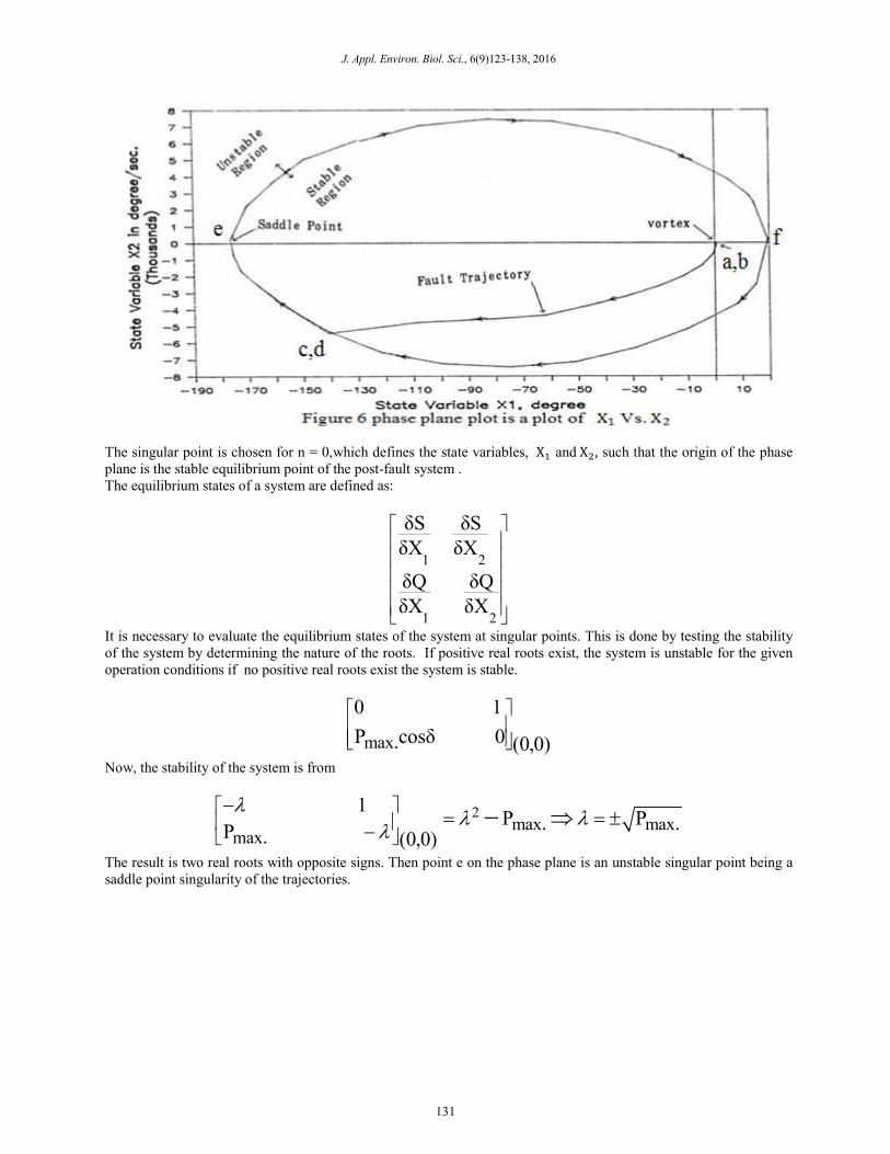
A phase plane plot is a plot of X� Vs. X� , as shown in Figure 6 . As the time t increases the two- tuple [ X�(t), X�(t)] describes the trajectory in the phase plane . Since stability of the postfault system is the basic issue of concern,

finding the stable equilibrium point (the origin of the phase plane) is important, since this point is the steady state

value for postdisturbed system.

1

1

1 2

2 12 1

1 2 2 2

2 12 1

2 12 1

S

X

S

X S

The state equation for the post-fault system is :

X X (21)

X P P P (X ) M (22)c max.m

Since X X X X (23)

X P P P (X ) Mc max.m

X P P P (X ) M c max.m

in

S ,

in

Q , in

( )

( )

.

. .

.

. .

.

φ

φ

φ

=

= +

= =

= +

= +

− −

⇒

− − ⇒

− −

( )( )

1

1

2 2

2 12 1

121

X

X S

(24)

Then the state equilibrium singular point is :

X 0 X 0 (25)

X P P P (X ) M 0 (26)c max.m

P Pcm(X ) arcsin (27)Pmax.

Where 0, 1, 2,.............

S ,

Q , in

( )

( ) .

n

n

φ

φ π

= =

= + =

+ =

=

=

⇒

− −

−

130

J. Appl. Environ. Biol. Sci., 6(9)123-138, 2016

The singular point is chosen for n = 0,which defines the state variables, X� and X�, such that the origin of the phase

plane is the stable equilibrium point of the post-fault system .

The equilibrium states of a system are defined as:

1 2

1 2

δS δS

δX δX

δQ δQ

δX δX

It is necessary to evaluate the equilibrium states of the system at singular points. This is done by testing the stability

of the system by determining the nature of the roots. If positive real roots exist, the system is unstable for the given

operation conditions if no positive real roots exist the system is stable.

max

0 1

P cosδ 0. (0,0)

Now, the stability of the system is from

2max max

max

1P P. .P . (0,0)

λλ λ

λ

−= = ±

−⇒−

The result is two real roots with opposite signs. Then point e on the phase plane is an unstable singular point being a

saddle point singularity of the trajectories.

131

Dghayes, 2016

( )

( )

1 2

2 12

1 2

2 12

S ss (Pre)

S ss (during)

The state equations for each system are :

Pre-fault system

X X (28)

X P P P ( ) M (29)c max.m

During fault system

X X (30)

X P P P ( ) M (31)c max.m

in

in

.

. .

.

. .

δ δ γ

δ δ γ

+

+

=

=

=

=

− +

− +

+

+

( )1 2

2 12S ss (Post)

Post-fault system

X X (32)

X P P P ( ) M (33)c max.m

in

.

. . δ δ γ +

=

= − + +

δ will decrease monotonically without bound beyond the maximum value possible for a marginally stable swing ,

δ%&'.

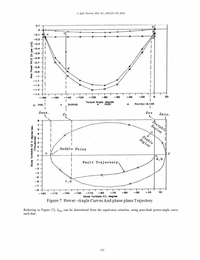
These equations are plotted in the phase plane with torque angle δ at its minimum value (δ%56. = 19° as indicated by

point f in Figure 7). Figure (7) illustrates the relationship between power-angle and the phase plane trajectories for a

marginally stable case . The prefault operating point (δ�, Pe�) is designated by the letter a in the figure, the power

system is in a state of equilibrium with ( and d/d"= 0), this point in the phase plane is a stable singular point called

a stable node or a vortex. When the 3-phase fault occurs at t ="�7 , the electrical output power of the system Pe��

increases to a value corresponding to point b , this results in a decrease in speed deviation d/d" the and the torque

angle . This decrease is depicted in the phase plane fault trajectory between δ�, and δ� . In the marginally stable

case , fault clearing is delayed long enough to permit the system torque angle to decrease to the critical value δ� at

which time the faulted line is isolated from the system. For fault clearing torque angles greater than δ� , the post-fault

system will be unstable . At the time the fault is cleared (at t =0.1 sec. corresponding to = δ� ) the output pover

Pe�� decreases from the value of −0.5 to −0.85 p.u , continues to decrease along the phase plane post-fault

trajectories from point c and d (at which = δ� ) toward point e . Point e ( = δ%&'. ) is an unstable singular point

which is saddle point of the trajectories. For a the conservative system under study, as increases a path is then

formed along the phase plane maximum trajectory in clockwise direction from point e to point f as show in the Figure

7 .

132

J. Appl. Environ. Biol. Sci., 6(9)123-138, 2016

Referring to Figure (7), δmin. can be determined from the equal-area criterion, using post-fault power-angle curve such that:

133

Dghayes, 2016

( )

( )( )

( )( )

( )

12

12

min.

ss

S(Post)

min.

max.

S(Post)

ss

max.

ss

P P P ( ) dδ (34)c max.m

P P ( ) P dδ (35)c max. m

Let X dx = dδ

0.167 1.12SinX+0.1452 dx = 02.16 p.u (36)

19 (0.332rad.) (37)

in

in

δ

δ

δ

δ

δ

δ

.

.

δ γ

δ

δ γ

δ γ

γ

γ

+

+ −

= ⇒

− + −

= °

+

− +

= +

∫

∫

+∫+

The critical clearing timetcr can be determined from (9), using numerical integration techniques:

( )( )( )

12

12 12

12

12 12

12 C

δc

crδ

δ0

aδ0

δc

crδ

δ0

m eδ0

S(dur.)

Se

0 0

δ

crδ

δ0

m 0 max. 0δ0

dδt (38)

2P dδ

M

dδt (39)

2P P dδ

M

Where

(40)c max.e

dδ= P P P ( ) dδ (41)c max.m

dδ t

2P P +P

M

P P P in

in

δ cos δ

δ δP

δ δ

.

. ( )

. ( )

.

. ( )( ) (cos )δ δ

δ γ

δ γ

+

+

=

=

=

− −

+

− +

∫∫

∫−∫

=

∫ ∫

−∫

c

cr

(42)

t 0.1 second=

∫

134

J. Appl. Environ. Biol. Sci., 6(9)123-138, 2016

2.8 STABILITY BOUNDARY

The system is considered stable as long as the trajectories follow the separatrix determined by the phase plane

(as shown in Figure 6). The equation for the separatrix can be determined from the post-fault system differential

equation of motion:

2

12 12 122

2 2 2

2

2 2

2

2

2

M P P P (43)a m e

Since 2 2 (44)

1Then (45)

2

Substituting Eq. (45) for in Eq. (43), the differential one

d

dt

d dδ dδ d dδ dδ d. . d. dδ

dt dt dt dt dt dt dt

d dδ d. .dδ dt dt

d

dt

δ

δ

δ

δ

.

= =

= =

=

⇒

−

( )( )

( )( )

2

12

2

12

S

S

-form is obtained.

MP P P (46)c max.m

2

2P P P (47)c max.mM

d dδ. . in dδ dt

dδd. in dδ

dt

.

.

δ

δ

=

=

− +

− +

( )( )1 2

22 12 1 1

S +

In term of the state variable , X and X

2P P P X dX (48)c max.mM

d(X in(

,

) ) . φ= − +Integration is performed to obtain the general solution for a post-fault system phase plane trajectory:

( )( )22 12 1

S +2

X P P P X + C = 0c max.mMin( ) . φ− − +

The constant of integration c is evaluated at the saddle point of the separatrix , which is (δmax. – ϕ ,0) .

12

2C = (P P P Cos (49)c max. max. max.mM

)() .δ φ δ − +−

The stability boundary of the post-fault system , is

( )22 12 1 1 1

12

S +2

P X P X P Xc max.mM2

(P P P Cos (50)c max. max. max.mM

in(

)

X ( ) ( ) )

(

.

) .δ φ δ

φ

+

− − +

− +−

( )

22 12 1

1

1

+

2(P P Xc max.mM

P Cos Cos X (51)max. max.

(52)max.min.

and )

(

) X )

X (

)

(

)

.

[

]

δ φ

δ

δ φ δ φ

φ

+ −−

+

−

−− ≤ ≤ −

The results obtained by this method agrees with that determined by the equal-area method.

135

Dghayes, 2016

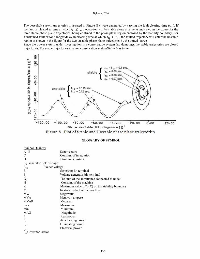
The post-fault system trajectories illustrated in Figure (8), were generated by varying the fault clearing time (tfc ). If

the fault is cleared in time at which tfc ≤ tcr , operation will be stable along a curve as indicated in the figure for the

three stable phase plane trajectories, being confined to the phase plane region enclosed by the stability boundary. For

a sustained fault or for a longer delay in clearing time at which tfc > tcr , the faulted trajectory will enter the unstable

region as shown in the figure for the two unstable phase plane trajectories by the dotted curve.

Since the power system under investigation is a conservative system (no damping), the stable trajectories are closed

trajectories. For stable trajectories in a non conservation systemX(t)→ 0 as t→ ∞

GLOSSARY OF SYMBOL

Symbol Quantity

A , B State vectors

C Constant of integration

D Damping constant

EfdGenerator field voltage

Eex Exciter voltage

Ei Generator ith terminal

Ej Voltage generator jth, terminal

Gii The sum of the admittance connected to node i

H Constant of the machine

K Maximum value of V(X) on the stability boundary

M Inertia constant of the machine

MW Megawatts

MVA Megavolt ampere

MVAR Megaras

max. Maximum

min. Minimum

MAG Magnitude

P Real power

Pa Accelerating power

Pc Dissipating power

Pe Electrical power

P�mGovernor action

136

J. Appl. Environ. Biol. Sci., 6(9)123-138, 2016

PmMechanical power

Pmax.Maximum power transfer

p.u Per unit

rad. Radian

r State vector

Q, S Liner operator

Sec. Second

t Time

tcr Critical clearing time

tfcFaultCritical clearing time

ω Machine speed in rad. /sec.

X State vector

X1 State variable in deg.

X2 State variable in deg. /sec.

X;q Direct-axis transient reactance

XT Transformer reactance

XL Transmission line reactance

Yij Admittance between node i and node j

ZL Load impedance

α ,β Completing the square constant

ϕ The sum of the steady-state torque angle and the real

component of transfer admittance

γ The real component of the transfer admittance Y12

$ System torque angle

δ� Angular speed deviation

$< Acceleration

$0 Predisturbed system $

$$$$. Minimum value of $ for a marginally stable condition

$$$$.Maximum value of $for a marginally stable swing

$$$Steady-state torque angle

π Pi=3.141592654 rad.

θijAngle between node i and node j

λ Engenvalue

Subscripts

1 Denotes to generator one

2 Denotes to generator two

12 Denotes the system equivalent power value

0 Denotes pre-fault system value (degree or initial)

SS Denotes the steady-state post-fault system value

2.8 CONCLUSIONS

The power system stability boundary for the two-finite machine system scheme, resulting knowledge gained from

system which has been studied in this paper, allows a number of general conclusions to be drawn concerning the

effect on stability of certain concepts used in power system design, apparatus design, and power system operation .

The effect of system modifications must be analytically observed before a fault, during a fault, and after fault

clearance. Experience has shown that some design changes improve stability during all three conditions, while other

modifications are helpful during one condition and detrimental during other changes.

Both methods studied in this paper, are compared and the final approaches giving identical results for the simplified

model. These two methods equal- area criteria and phase-plane trajectory, however, are suitable for a two-machine

system. There is still much further research can be done using stability analytical tool known as the second or the

direct method of Liapunov for getting a larger, more accurate, region of stability boundary of power system.

137

Dghayes, 2016

REFERENCES

1. Anderson, P.M., and A. A. Fouad, Power system control and stability, vol.1. The Iowa State University

Press, Ames. Iowa, 1977

2. Stevenson, D., Elements of Power System Analysis 4th Edition Mc Graw-Hill, New York, 1982.

3. Gless, G.E. The Direct Method of Liapunov Applied to Transient Power system IEEE Transactions. PAS-

85, 1966.

4. Wall, E.T. "A Topological Approach To The Generation of Liapunov Functions." Acta Technica Csav,

Prague, Czachos lovakia, No.2, 1968.

5. Roemish, W.R. A New Synchronous Generator Out-of-Ste Relay scheme Ph.D. Dissertation, University of

Colorado At Boulder, 1981.

6. Meyer, J.c. Control Principles And Application Modern

McGraw-Hi11 New York, 1968.

7. Jordan, D w., and P.Smith, Non Linear ordinary Differential Equations

2nd edition. Oxford University Press, New York, 1987 of control systems,

8. Ogata, K., State-Space Analysis of Control System, Prentice-Hall. Englewood cliffs, N.J. 1967.

138