The boundary layer on a finite flat plate - Massey Universityrmclachl/PFA91.pdf · The boundary layer on a finite flat plate Robert I. McLachlan*) Appiied Mathematics, ... boundary-layer

The boundary layer on a finite flat plate Robert I. McLachlan*) Appiied Mathematics, California Institute of Technology, Pasadena, California 91125

(Received 19 June 1990; accepted 22 October 1990)

The problem of finding the flow over a finite flat plate aligned with a uniform free stream is revisited. Multigrid is used to obtain accurate numerical solutions up to a Reynolds number of 4000. Fourier boundary conditions keep the computational domain small, with no loss of accuracy. Near the trailing edge, excellent agreement with first-order triple-deck theory is found. However, previous comparisons between computations, experiments, and triple-deck theory are shown to be misleading: In fact, triple-deck theory only accounts for half the drag excess (that part not due to the first-order Blasius boundary layer) even at R = 4000. The remainder is shown to be due to, among other things, a large displacementlike effect in the boundary layer, i.e., an O(R - ’ ) increase in skin friction extending over the whole plate.

I. INTRODUCTION

The problem of determining the flow of an incompress- ible, slightly viscous fluid over a finite flat plate aligned with a uniform free stream is literally a textbook example in boundary-layer theory. Unlike the flow past a semi-infinite plate, which is now understood and is discussed in Van Dyke,’ the finite plate is considerably more complicated because of the multistructured wake and its upstream influence. Van Dyke also reviews this problem, but our study suggests that previous workers were too hasty to declare the problem closed. As an example of high-Reynolds-number flow, the flat plate at first appears to be about the simplest problem one could think of. Both the zeroth-order solution (no disturbance to the free stream) and the first-order solution (the Blasius boundary layer followed by a Goldstein wake) are known. Thus, problems such as selecting one of a multiplicity of Euler solutions as the inviscid limit, which must normally be considered in dealing with high-Reynolds- number flows, are not present here. Difficulties arise at the next order, where a multitude of competing effects appear, and when we try to explain results from finite-Reynolds- number calculations.

In the course of an investigation of triple-deck phenom- ena (see McLachlan2*3 ), we turned to the finite flat plate as a case in which it was known to apply. Great success for triple- deck theory is often claimed here-for example, Jobe and Burggraf s4 Fig. 4 comparing drag coefficients is frequently reproduced (for example, in the review by F. T. Smith’). The theory at first appears to be easy to test in this case because it has no undetermined constants. Here, the triple deck is established around the trailing edge and gives the upstream effect on the boundary layer of the singular near wake, with a contribution to the drag of 2.66R - “‘, where R is the Reynolds number based on the free-stream speed and the length of the plate. This correction to the Blasius drag agrees with Navier-Stokes calculations (Jobe and Burg- gra?). However, prior to the discovery of the triple deck, the second-order theory of Kuo,~ which gives the correction to the first-order drag as 4.12R - ‘, also seemed to be in agree-

“‘Present address: Program in Applied Mathematics, Campus Box 526, University of Colorado at Boulder, Boulder, Colorado 80302.

ment. Furthermore, a glance at the results of Dennis and Dunwoody’s 1966 finite-Reynolds-number calculations’ shows that neither theory accounts for the calculated values of the skin friction on the plate. We decided to do some Navier-Stokes calculations ourselves to see what was really going on.

It turns out that finite-Reynolds-number results are greatly influenced by the small viscous regions at the leading and trailing edges in which the full Navier-Stokes equations hold. At moderate Reynolds numbers ( < - lOOO), these make it impossible to see any triple-deck trailing-edge region directly. However, by obtaining accurate solutions to the full Navier-Stokes equations up to a Reynolds number of 4000, and by constructing a least-squares fit between the numerical data and a model theory, we can show that triple-deck theory is consistent with the data. One reason that the triple deck’s trailing-edge effect [of streamwise extent 0( R - 3’8) ] is not obvious is that there is a large displacementlike effect in the boundary layer, i.e., an 0( R - ’ ) increase in skin friction extending over the whole plate. For example, at R = 600, this is comparable in magnitude to the triple-deck effect. An O(R - ‘) increase would correspond to the influence of changes in the external flow caused by the Blasius ’ boundary layer.

Finally, we construct a model of the flow that includes all these effects, and show that the apparent agreement in drag found by previous workers is, in fact, a coincidence that is due to near cancellation of the next smallest terms of the drag expansion.

II. HISTORY AND OVERVIEW

We consider the two-dimensional motion of an incom- pressible, Newtonian fluid. Let the free stream be given by I( = 1, u = 0 at infinity, and let the flat plate lie on the x axis between x = 0 and x = 1; then the Reynolds number R is given by l/v, where Y is the kinematic viscosity of the fluid. The flow is sketched in Fig. 1. The leading-order behavior of the boundary layer (valid in region IV of Fig. 1) was given by Blasius:’ The local skin friction is c B, = R - ‘uy (x,0) = A(x/R) - I”, where ;1 = 0.332 06, and the normalized drag coefficient is Da, = 4ilR - 1’2.

341 Phys. Fluids A 3 (2), February 1991 0899-8213/91/020341-08$02.00 @ 1991 American Institute of Physics 341

IX

0 X - Ef -

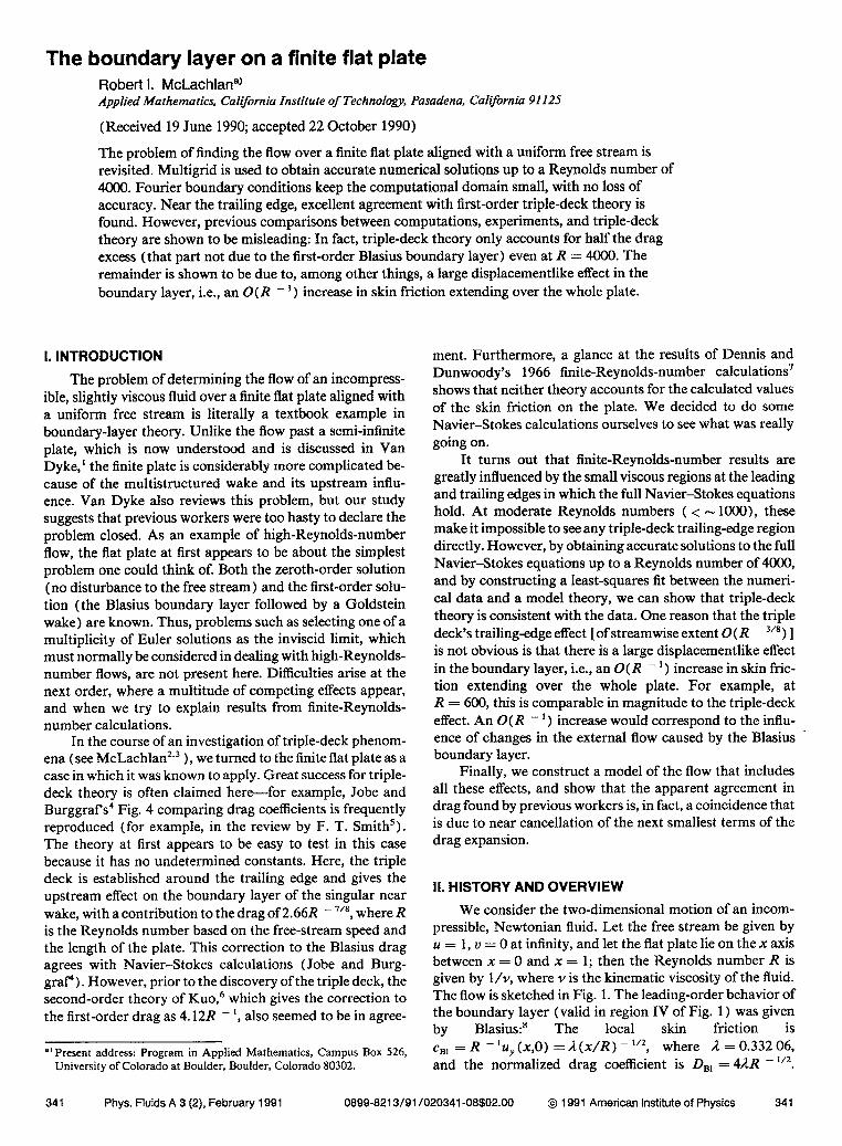
FIG. 1. Schematic flow structure. Here, e = R -I’s is the small parameter. In each indicated region, distinct approximations to the Navier-Stokes equations are valid. I. Viscous sublayer; boundary layer equations hold. Ii. Continuing Blasius boundary layer; inviscid with vorticity. III. Potential flow, O( 8) perturbation to free-stream velocities; linearized Euler equations hold. IV. Blasius boundary layer. V. Potentiai flow, O(8) perturbation to free-stream velocities; tends to uniform flow at infinity. VI. and VII. Fully viscous, Navier-Stokes equations hold. VIII. Goldstein sublayer,vertical extend 8(x - 1 )I”, similarity solution valid for x - 1 Q 1, IX. Far wake, vertical extent 8(x - 1 )‘I’, similarity solution for x - 1% 1.

These formulas are valid when x$R - I”, close to the leading edge, when x = 0( R - ’ ) (region VI), the boundary- layer approximation is not valid, and a full Navier-Stokes solution is required. This was calculated numerically by Veldman and van de Vooren,’ who found that the skin friction near the leading edge is about 13% larger than the Bla- sius value. Note that these two regions unfortunately do not formally overlap, so that analytic matching is not possible.

We express the skin friction and drag relative to their Blasius values as follows:

r=&~,(x,O) and D=- - l 2 ludx s D,, R o JJ ’

(1)

Goldstein” analyzed the wake just behind the plate, and found a two-tiered structure, consisting of the continuing, initially unchanged Blasius layer, and an inner layer (region VIII), required because of the change in boundary conditions at x = 1, in which u(x,O) grows like (x - 1) “3. For downstream, these two layers merge (again not formally overlapping) in region IX, where the flow has a similarity form.

Kuo” attempted to find the next term in the boundary layer on the plate by assuming that the vertical velocity at the outer edge of the boundary layer is zero in x > 1. The displacement effect of the first-order boundary-layer on the external flow can then be calculated, and finally the boundary- layer equations reintegrated with this new external flow, This procedure gives the second-order skin friction and drag as

upstream influence of Goldstein’s sublayer is of streamwise extent O(R - ‘/*), and is described by a triple deck established around the trailing edge, Most of the Blasius layer continues largely unchanged except for a small vertical displacement (region II). Pressure perturbations in the external flow (region III) of order R - *” are coupled to a thin, viscous sublayer next to the plate (region I). There is an additional buffer region (not shown) established around the trailing edge, in which the pressure varies withy; details are in Messiter.” Full details of the matched asymptotic expansion that leads to the triple-deck structure are available else- where, for example in Stewartson’s review. I3

The lower deck has vertical extent 0( R - 5’8) and velocities 0( R - I’*); hence the skin friction is 0( R “‘*) there, just as in the Blasius boundary layer, The equations that hold in the lower deck are the same as those found in laminar separation, but the boundary conditions at y = 0 and as Ix 1 ,y + 03 are different, Also, because the limiting solution is known, there are no free parameters left in the equations or the scalings. This simplifies matters considerably, and the lower-deck equations were solved by Jobe and Burggraf,4 and later by Veldman and van de Vooren’and by Melnik and Chow,14 who found

7- = 1 =+ &T(X), D = 1 f 2.OOR - 3’8, (3)

where X = /z 5/4R 3/8(x - 1) is the inner length. (The fi term arises from our definition of 7. ) Jobe and Burggraf, like Kuo, reported excellent agreement with the drag, down to a Reynolds number of one (!). They reported that Dennis and Dunwoody’ bad found evidence in their Navier-Stokes solutions that supported the existence of an R - 3’8 region, and had even confirmed the value of T(O). This is difficult in view of the singularity in skin friction present at the trailing edge on the smallest 0( R - 3’4) scale analyzed by Stewart- son.” Since (2) and (3) are in conflict, they suggested that the O( II - ’ ) term in (2) was canceled by further terms in the triple-deck expansion.

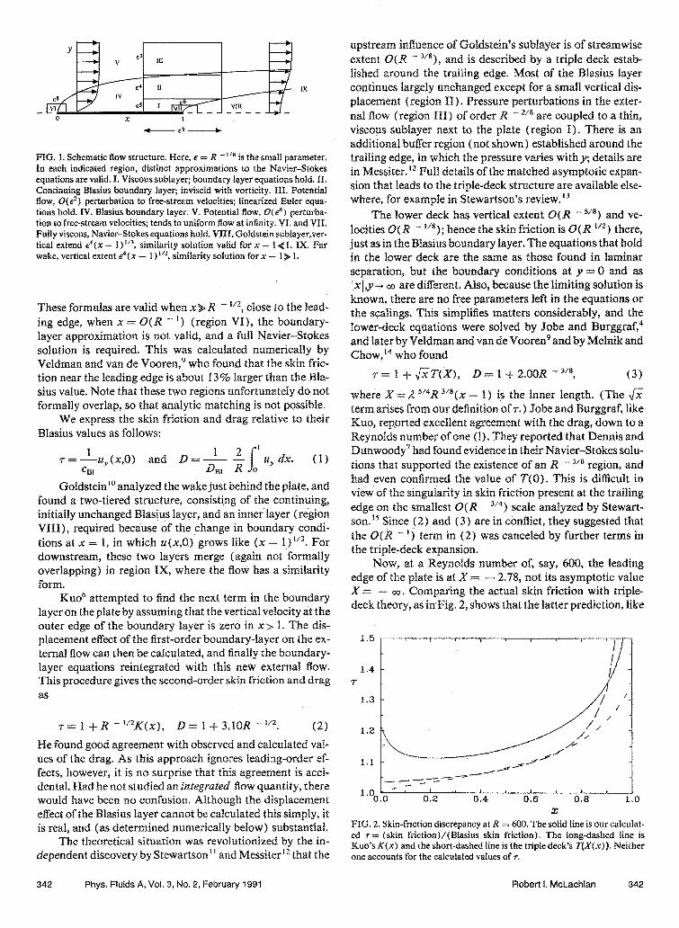
Now, at a Reynolds number of, say, 600, the leading edge of the plate is at X = - 2.78, not its asymptotic value X = - CO, Comparing the actual skin friction with triple- deck theory, as in Fig. 2, shows that the latter prediction, like

T= 1 +R -“2K(~), D= 1 +3,10R -“2. (2) : He found good agreement with observed and calculated values of the drag. As this approach ignores leading-order effects, however, it is no surprise that this agreement is a&i- dental. Had he not studied an iategruted flow quantity, there would have been no confusion. Although the displacement effect of the Blasius layer cannot be calculated this simply, it X

is real, and (as determined numerically below) substantial. FIG. 2. Skin-friction discrepancy at R = 600. The solid line is our calculat-

The theoretical situation was revolutionized by the in- ed r= (skin friction)/(Blasius skin friction). The long-dashed line is

dependent discovery by Stewartson” and Messiter” that the Kuo’s iu(x) and the short-dashed line is the triple deck’s &Y(x)). Neither one accounts for the calculated values of 7:

342 Phys. Fluids A, Vol. 3, No. 2, February 1991 Robert 1. McLachlan 342

Kuo’s is also too small by a factor of about 2. The accidental agreement in drag must come from the inclusion in the inte- grated skin friction of the range from - 00 to the leading edge.

III. COMPUTATIONS The skin friction results of Dennis and Dunwoody are

sufficient to show that all is not well, but it is hard to extract detailed information from their graphs. We decided to solve the Navier-Stokes equations for a range of Reynolds numbers using an existing multigrid program. The great ad- vantage of multigrid is that both memory and computation time are linear in the number of unknowns, so that very fine grids can be used. However, at high Reynolds numbers, spe- cial techniques must be used to ensure rapid convergence and to prevent unwanted numerical diffusion from creeping in. Our experiences with various upwinding and defectsor- rection schemes are reported in McLachlan.2p’6 Rapid, grid- independent convergence can be obtained (with error reduc- tions, in this case, ofabout 0.2 per iteration) to solutions that are O( h ‘) accurate in the mesh spacing h. Errors are reduced below truncation errors in 3 or 4 iterations, with a total work requirement equivalent to about 30 Gauss-Seidel relaxations.

We use the stream function-vorticity representation of the flow, in which the velocities are related to the stream function 11, by u = *;,v = - $X and the vorticity w is de- fined by o = v, - u,,. Nondimensionalizing lengths by the length of the plate L and velocities by the undisturbed free- stream speed U, the Navier-Stokes equations for incom- pressible, steady flow are

v**= -w, (4) . . V20 = Rt$p, - $.p,,,

where the Reynolds number R = U& /Y, and v is the kinematic viscosity.

The desired high-order correction to the skin friction is caused by the upstream influence of the wake. We must therefore have an accurate solution for the flow not only on the plate, but in a large part of the wake, and also in the far field, through which upstream influences are transmitted. Parabolic coordinates are almost always used in flat-plate studies because, then, the wake remains of constant thick- ness as l-+03. There is also a moderate (quadratic) grid expansion in the far field and a contraction near the singular leading edge. Unfortunately, the grid is regular at the trailing edge, where the flow is singular. We return to this point below.

Let x=6*-7*, y=2&7 (5)

so that Eqs. (4) become

v’+ = - J(&#‘h

V2w = R($,p5 - $.p, 1, (6)

where J(E,v) = 4(c2 + v2) is the Jacobian of the transfor- mation and now V2 = a,, + d,,. The half-plane y>O maps to the quarter plane g,~>0, with the plate at O<x< 1, y = 0

mapping to 0~6~ 1, 7 = 0. The boundary conditions are

*=o, on {=O and on v=O, (7a) w=O, on g=O and on ~=0, g>l, G’b) qv =0, on ~=0, OCcCl, (7c) ++y,w-+O, as &,rl+ 00. Ud)

In practice, we use the perturbation stream function $ - y as the unknown, which results in trivial modifications to the equations and boundary conditions.

Conditions (7a) and (7b) can be imposed directly. The no-slip condition (7~) is transformed using the Woods” expansion, replacing it with a boundary condition for the vorticity:

(Jm) (&O) = (3/k2)?Mk) - $(Jo) Gk). (8)

Here, k is the mesh spacing in the 77 direction. The far-field condition (7d) is the most problematical. The domain is truncated at finite values g, and 77,) and we want to ensure that the values used have an effect on the solution that is less than the truncation error. Simply imposing the free- stream flow (7d) violates conservation of momentum and leads to large errors at the plate. Using the OseCn wake, given by Imat, ’ l8 which models the downstream wake and the sink inflow required to balance it, is not much better. Fornberg” has pointed this out in his study of the flow past a cylinder. In that case, there is a large irrotational effect in the far field caused by the trailing eddies. Here, even though there are no eddies, we have the same problem: The perturbation to the free stream decays to the Osekn source term very slowly. For example, in our case, the ratio of the second- to the first- order correction to the free stream at a distance r from the plate can be up to 0.26r- I”. Higher-order terms include powers of log r and r - I”; moreover, the radius of convergence of the OseCn expansion has not been established. With an OseCn boundary condition, although we found it possible to increase the domain to the point where the effect of domain truncation appeared to be less than the discretization error at the plate, the solution was of course not uniformly valid throughout the domain-an unsatisfactory state of af- fairs.

Fornberg19p20 has proposed and successfully used an accurate and economical alternative. Because the vorticity decays exponentially away from the plate (unlike the perturbation to the free stream), the stream function satisfies Laplace’s equation to a high degree of accuracy in the far field-in ~7 > r], , say. Laplace’s equation can be solved by Fourier decomposition in the domain 6 > 0, ~7 > V, - k, and the solution written down at 37 = 7, . This gives a boundary condition for the stream function at the outer boundary in terms of its values at the adjacent interior points. In this way, the computational domain need only cover that portion of the flow that contains vorticity-in our case, an O( R - “2) layer next to r] = 0. On an infinite 5 domain with mesh spacings h, k in the 6, v directions, A = k/h, and k&f = 7, , the result (from Fornberg*‘) is

$i,M = 9 cli-jl $j,M- 1) j= --m

343 Phys. Fluids A, Vol. 3, No. 2, February 1991 Robert I. McLachlan 343

where

I

2a ck= e- 2rl Sin(d*)COS kz &we (10)

0

Fornberg gives an asymptotic expansion of ( 10) valid for large k.

In parabolic coordinates, there is also a downstream cutoff at g = 6, . Fornberg** neglected the streamwise de- rivatives and used the equation $9v = - Jw there. Kow- ever, in our iterative solver, treating this as a two-point boundary-value problem with $(l, ,O) and $(t, ,YJ- ) as boundary conditions was not successful. Large components linear in 7 would enter tl, and feed back (through the top Fourier boundary condition) into the solution, destroying convergence.

The first-order OseCn expansion has @< = 0 in the wake. Comparison with numerical solutions (see Fig. 4) shows that this is in fact highly accurate throughout the wake, even quite close to the plate. It is not formally valid outside the wake, but as the domain does not extend far in this direction, we use it for all r and check later that the g cutoff does not affect the solution. With qf: = 0 we obtained rapid convergence.

Far-field boundary conditions for the votticity are not crucial. The largely parabolic nature of the vorticity trans- port equation means that errors are not transmitted far upstream. (For example, even setting WC{, ,T) = 0 only af- fects the solution a few grid points upstream. ) We set w = 0 on the top boundary, and impose the asymptotic decay of vorticity downstream: w a 6 - 2.

The boundary condition $( 0,~~ ) = 0 can be incorpo- rated in (9 ) by an odd extension of $ into 6 < 0. At the right- hand boundary, we assume that $p = 0 in {, <g< ~4 and evaluate the infinite sum in (9) using d, = 2,~~ k~j; we found dk from the asymptotic expansion of the cj’s. On an N XM grid, Eq. (7d) is therefore implemented as

$t,M = (dN-j -dN+j)ZltN,M- t N-l

+ 2 Cc[i-jl -Ci*j)+j,M- It 'GiGN? j= I

(lla)

3Nj = *N- ,j, lGi<M (Ilb) @i,M = 0, l<i<N, (llc)

@NJ = [tj- l>/jl*W,- ,j, lG<M. (lid)

Although imposing ( 1 la) takes time O(NM), this is still negligible compared to the time spent on the interior equations.

All of our final computations used 4, = 4, or x m = 16. Clearly it is inefficient to cover the whole domain with a uniformly fine grid, because most of the activity in the flow field occurs near the plate. In multigrid, this problem can conveniently be avoided by only relining the grid in a subdomain, or in a set of subdomains. Ideally, one would like to minimize the discretization error for a given amount of computational work; however, the multitude of possibilities (nested subdomains, etc.) preclude this. We first ascer- tained that two refinements in [0, I.41 X [0, v, ] gave almost the same accuracy as two refinements covering the

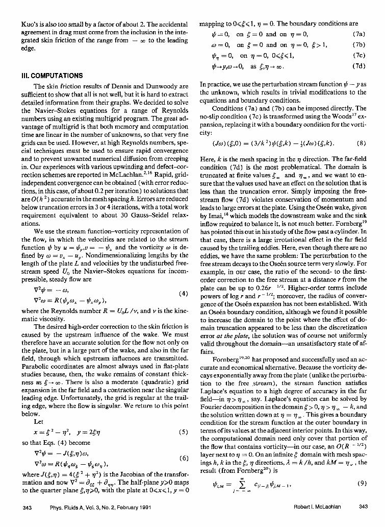
whole domain, but that, with further refinement, accuracy was limited by the unrefined part of the domain. Then we kept the two-refinement strategy fixed and tested the overall accuracy by halving the mesh spacing over the entire domain (subdomains included). A sample domain is shown in Fig. 3.

The finest grids used had N = 256 grid points in 0+$<4 and M= 64 points in O<q<v,. The finest subdomain had 360 points in OC&-< 1.406 (or 256 points on the plate) and 120 points vertically. (The subdomain stopped a few grid points short of 7;1, for ease of implementing the Fourier boundary condition.) We generally took 17, - 5R - lit, which assured that 101 < 10e4 at 7 = 71, - k [where the boundary condition ( 1 la) is evaluated] for all ,$. (If the domain was any smaller, the vorticity did not decay exponentially for large 7.) At R = 600, increasing (4, ,q, ) from (4,0.2) to (4,0,3), (4,0.4), and (5,0.2) (keeping the mesh spacings constant in each case) altered the drag by less than 0.005%. In fact, 6, could be reduced to 2 before the domain truncation error became comparable with the discretization error on the finest grid. The Fourier boundary condition ( 1 la) is thus extremely successful at allowing reduction of the computational domain, while the outflow condition ( 1 lb) does not significantly affect the solution. In addition, the decrease in vertical mesh size k as the Reynolds number increases stops the errors growing rapidly. Here, we found that the relative discretization error in the drag grows roughly like R o.5, in contrast to the R ‘,5 growth seen with constant mesh sizes. As the grid aspect ratio ;E decreases (to 0.08 at R = 4000), the anisotropy of the grid slows the asymptotic convergence rate of our multigrid algorithm. This could be avoided by using line instead of point relaxations on v*qfl = - fw. However, as the initial rapid convergence was not affected, it was easiest to just run a few more iterations. Twelve iterations always gave convergence to within a few percent of the discretization error.

Far downstream, the wake rapidly assumes the Gold- stein form. The near wake is more problematical, and, in fact, at the Reynolds numbers considered, there is no clear region in which the u (x,0) -xt, I” Goldstein similarity solution dominates. For moderate xt, = x - 1, higher-order terms (x::” etc. ) are significant and there is a smooth recov- ery of the flow to tt = 1 downstream; but for x,, -0, the full Navier-Stokes equations apply and u(x,O) -xl,‘” instead. The expected scaling (see Sec. IV) was verified and we fmd

I-

1 Y 1

FIG. 3. Computational grid. Shown here for Re = 1000, N = 32,6, = 4, ,and 7t, = 0.142. The actual finest grid used has 1 the mesh spacing everywhere.


u&,0) = R "4X;c/2[O.46 - 0.027X,, + 0 (XQ)], (12)

whereX,, = R 3'4 (x - 1). We therefore studied the flow on the plate in detail rather than the wake.

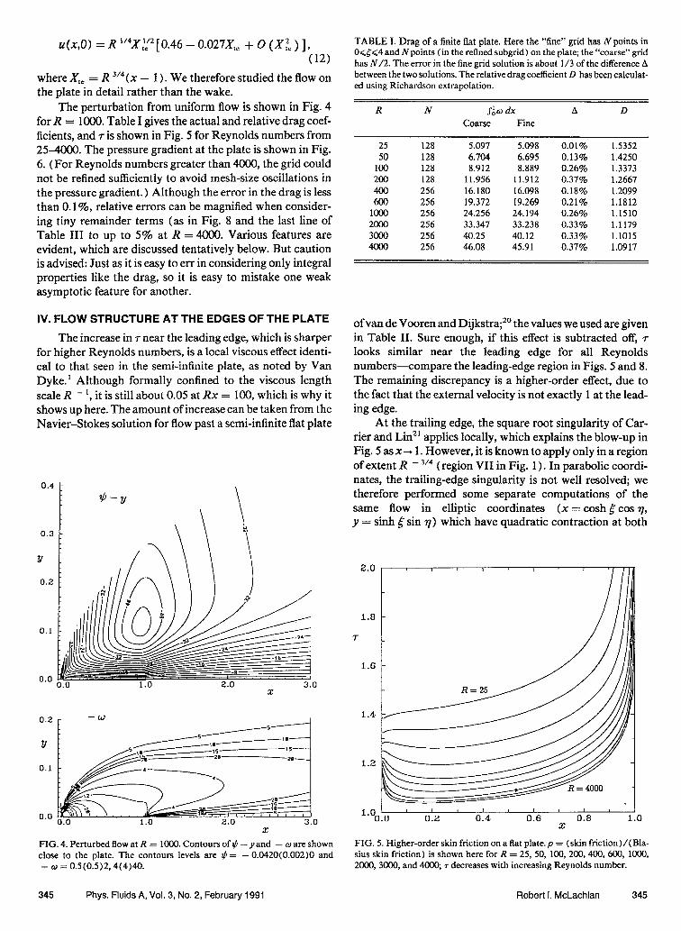
The perturbation from uniform flow is shown in Fig. 4 for R = 1000. Table I gives the actual and relative drag coefficients, and r is shown in Fig. 5 for Reynolds numbers from 25-4000. The pressure gradient at the plate is shown in Fig. 6. (For Reynolds numbers greater than 4000, the grid could not be refined sufficiently to avoid mesh-size oscillations in the pressure gradient.) Although the error in the drag is less than 0. l%, relative errors can be magnified when considering tiny remainder terms (as in Fig. 8 and the last line of Table III to up to 5% at R = 4000. Various features are evident, which are discussed tentatively below. But caution is advised: Just as it is easy to err in considering only integral properties like the drag, so it is easy to mistake one weak asymptotic feature for another.

IV. FLOW STRUCTURE AT THE EDGES OF THE PLATE

The increase in r near the leading edge, which is sharper for higher Reynolds numbers, is a local viscous effect identi- cal to that seen in the semi-infinite plate, as noted by Van Dyke.’ Although formally confined to the viscous length scale R - ‘, it is still about 0.05 at Rx = 100, which is why it shows up here. The amount of increase can be taken from the Navier-Stokes solution for flow past a semi-infinite flat plate

Y

0.2

0.1

0.0 0.0 1.0 2.0 3.0

0.2

Y

0.1

0.0

xi

-W

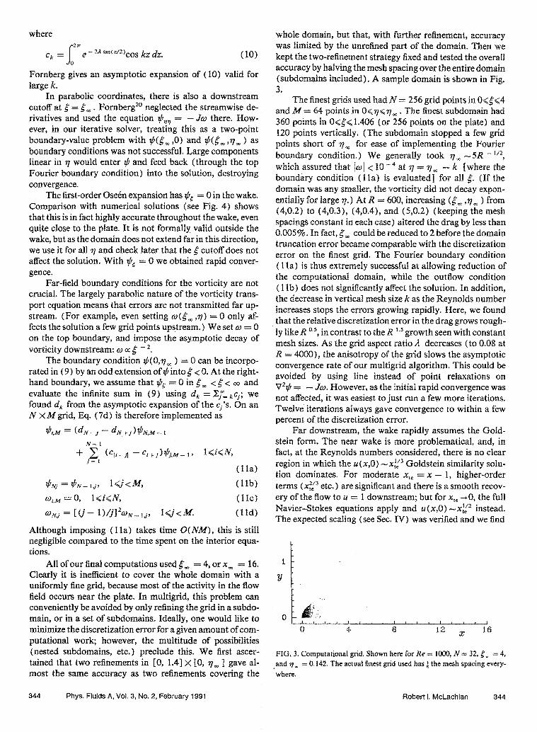
FIG. 4. Perturbed tlow at R = 1000. Contours of $ - y and - o are shown FIG. 5. Higher-order skin friction on a flat plate. p = (skin friction)/(Bla- close to the plate. The contours levels are $ = - 0.0420(0.002)0 and sius skin friction) is shown here for R = 25, 50, 100, 200,400, 600, 1000, - o = 0.5(0.5)2,4(4)40. 2000, 3000, and 4oo0, r decreases with increasing Reynolds number.

TABLE I. Drag of a finite flat plate. Here the “fine” grid has N points in 0<<<4 and Npoints (in the refined subgrid) on the plate; the “coarse” grid has N/2. The error in the fine grid solution is about l/3 of the difference A between the two solutions. The relative drag coefficient D has been calculated using Richardson extrapolation.

R N $;o dx A D Coarse Fine

25 128 5.097 5.098 0.01% 1.5352 50 128 6.704 6.695 0.13% 1.4250

100 128 8.912 8.889 0.26% 1.3373 200 128 11.956 11.912 0.37% 1.2667 400 256 16.180 16.098 0.18% 1.2099 600 256 19.372 19.269 0.21% 1.1812

loo0 256 24.256 24.194 0.26% 1.1510 2000 256 33.347 33.238 0.33% 1.1179 3ooo 256 40.25 40.12 0.33% 1.1015 40@3 256 46.08 45.91 0.37% 1.0917

of van de Vooren and Dijkstra;” the values we used are given in Table II. Sure enough, if this effect is subtracted off, r looks similar near the leading edge for all Reynolds numbers-compare the leading-edge region in Figs. 5 and 8. The remaining discrepancy is a higher-order effect, due to the fact that the external velocity is not exactly 1 at the leading edge.

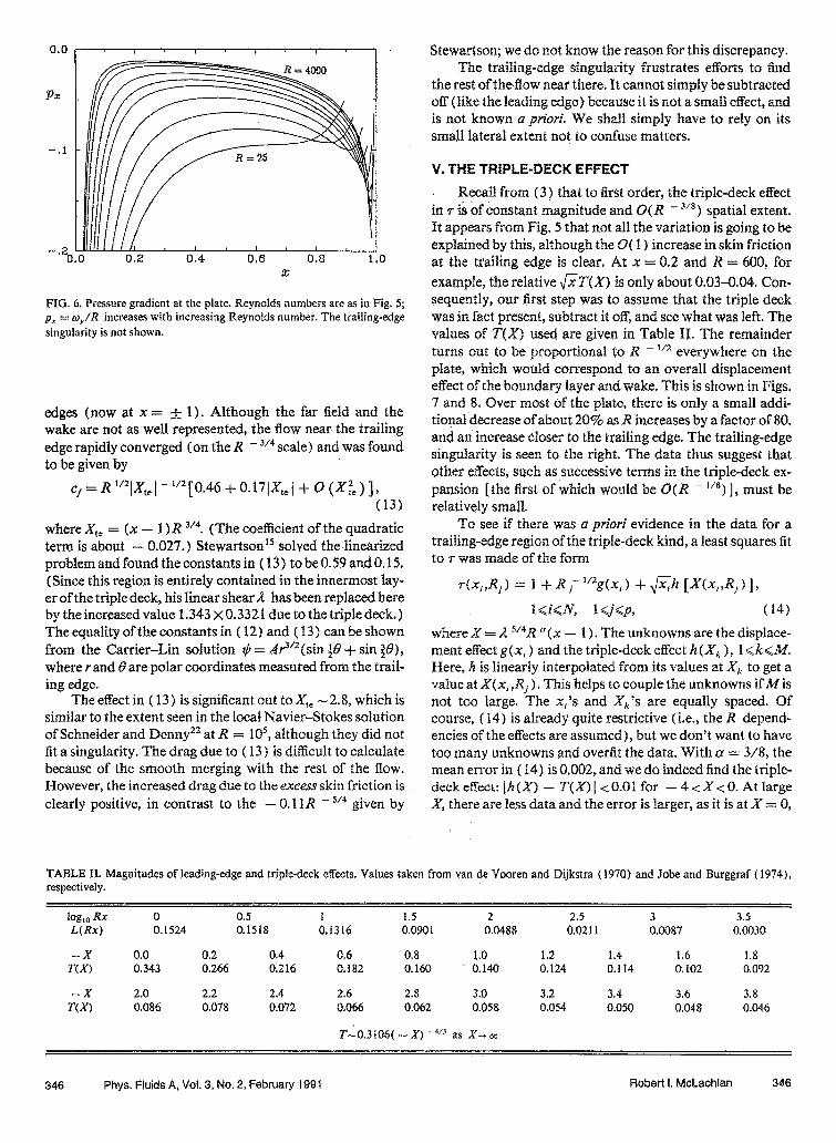
At the trailing edge, the square root singularity of Car- rier and Lin2’ applies locally, which explains the blow-up in Fig. 5 as x-r 1. However, it is known to apply only in a region of extent R - 3’4 (region VII in Fig. 1). In parabolic coordinates, the trailing-edge singularity is not well resolved; we therefore performed some separate computations of the same flow in elliptic coordinates (x = cash 5 cos 7, y = sinh g sin 7) which have quadratic contraction at both

2.0

1.8

7-

1.6

1.4


0.0

PX

-.l

-.2 C

I 1 1 b Stewartson; we do not know the reason for this discrepancy. The trailing-edge singularity frustrates efforts to find

the rest ofthetlow near there. It cannot simply be subtracted off (like the leading edge) because it is not a small effect, and is not known a priori, We shall simply have to rely on its small lateral extent not to confuse matters.

V. THE TRIPLE-DECK EFFECT

Recall from (3) that to first order, the triple-deck effect in r is of constant magnitude and O(R - “‘) spatial extent. It appears from Fig, 5 that not all the variation is going to be explained by this, altbough the 0( 1) increase in skin friction at the trailing edge is clear, At x = 0.2 and I? = 600, for example, the relative fir(X) is only about 0.03-0.04. Con- sequently, our first step was to assume that the triple deck was in fact present, subtract it off, and see what was left. The values of T(X) used are given in Table II. The remainder turns out to be proportional to R -1’2 everywhere on the plate, which would correspond to an overall displacement effect of the boundary layer and wake. This is shown in Figs. 7 and 8, Over most of the plate, there is only a small additional decrease of about 20% as R increases by a factor of 80, and an increase closer to the trailing edge. The trailing-edge singularity is seen to the right, The data thus suggest that other effects, such as successive terms in the triple-deck expansion [the first of which would be O( R - ‘I’) 1, must be relatively small.

FIG. 6. Pressure gradient at the plate. Reynolds numbers are as in Fig. $; px = w,,/R increases with increasing Reynolds number, The trailing-edge singularity is not shown.

edges (now at x = f 1). Although the far field and the wake are not as well represented, the flow near the trailing edge rapidly converged (on the R - 3’4 scale) and was found to be given by

where X,, = (x - 1) R 3’4. (The coefficient of the quadratic term is about - 0.027.) Stewartson” solved the linearized problem and found the constants in ( 13 ) to be 0.59 and 0.15, (Since this region is entirely contained in the innermost layer of the triple deck, his Iinear shear il has been replaced here by theincreasedvame 1.343 X0.3321 due to the triple deck,) The equality of the constants in ( 12 ) and ( 13 ) can be shown from the Carrier-Lin solution $ = &“(sin $0 + sin $9)) where r and 6 are poIar coordinates measured from the trailing edge.

The effect in ( 13) is significant out to X,, - 2.8, which is similar to the extent seen in the local Navier-Stokes solution of Schneider and Denny22 at R = lo*, although they did not tit a singularity. The drag due to ( 13) is difficult to calculate because of the smooth merging with the rest of the flow. However, the increased drag due to the excess skin friction is clearly positive, in contrast to the - 0.11 R - 5'4 given by

To see if there was a priori evidence in the data for a trailing-edge region of the triple-deck kind, a least squares fit to r was made of the form

r(xipRi 1 = 1 + R j- “‘g(X, 1 + J;;;h [X(X, ,Rj 11,

l<iSN, 1 gxp, (14)

whereX = /z 5’4t9 “(x - 1) . The unknowns are the displacement effect g(Jc;) and the triple-deck effect h(X, ), 1 <k<M. Here, fi is linearly interpolated from its values at X, to get a value at X(xi ,R, > t This helps to couple the unknowns if M is not too large. The x,‘s and Xkfs are equally spaced. Of course, ( 14) is already quite restrictive (i.e., the R depend- encies of the effects are assumed), but we don’t want to have too many unknowns and over& the data. With a = 3/8, the mean error in ( 14) is 0,002, and we do indeed tind the triple- deck effect: \h (X) - T(X) ] < 0.01 for - 4 < X < 0. At large X, there are less data and the error is larger, as it is at X = 0,

TABLE II. Magnitudes of leading-edge and triple-deck effects. Values taken from van de Yooren and Dijkstra ( i970) and Jobe and Burggraf ( 19741, respectively.

log,, Rx URx)

-x T(X)

-x T(X)

0 0.5 l i1316 1.5 2 3 3.5 0.1524 0.1518 0.0901 0,0488 0.0087 0.0030

0.0 0.2 0.4 0.6 0.8 1.0 1.2 1.4 1.6 1.8 0.343 0.266 0.216 0.182 0,160 0.140 0.124 0.114 0.102 0.092

2.0 2.2 2.4 2.6 2.8 3.0 3.2 3.4 3.6 3.8 0.086 0.078 0.072 0.066 0.062 0.058 0.054 0.050 0.048 0.046

T-0,3106( -X) -W as X-t CO

346 Phys. Fluids A, Vol. 3, No. 2, February 1991 Robert 1. McLachlan 346

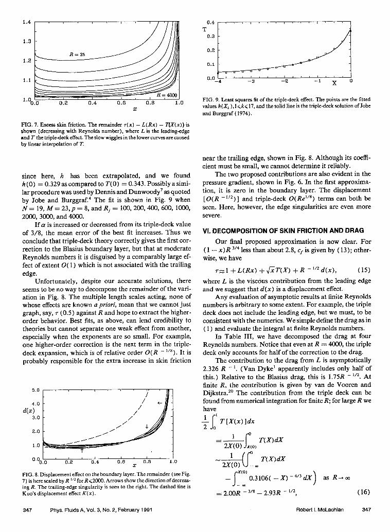
FIG. 7. Excess skin friction. The remainder T(X) - L(Rx) - Tcy(x)) is shown (decreasing with Reynolds number), where L is the leading-edge and T the triple-deck effect. The slow wiggles in the lower curves are caused by linear interpolation of T.

since here, h has been extrapolated, and we found fi (0) = 0.329 as compared to T( 0) = 0.343. Possibly a similar procedure was used by Dennis and Dunwoody’ as quoted by Jobe and Burggraf.4 The fit is shown in Fig. 9 when

If cz is increased or decreased from its triple-deck value of 3/8, the mean error of the best fit increases. Thus we

N= 19, M= 23,~ = 8, and Rj = 100,200,400,600, 1000,

conclude that triple-deck theory correctly gives the first correction to the Blasius boundary layer, but that at moderate

2000,3000, and 4000.

Reynolds numbers it is disguised by a comparably large effect of extent O( 1) which is not associated with the trailing edge.

Unfortunately, despite our accurate solutions, there seems to be no way to decompose the remainder of the variation in Fig. 8. The multiple length scales acting, none of whose effects are known a priori, mean that we cannot just graph, say, r (0.5) against R and hope to extract the higher- order behavior. Best fits, as above, can lend credibility to theories but cannot separate one weak effect from another, especially when the exponents are so small. For example, one higher-order correction is the next term in the triple- deck expansion, which is of relative order 0( R - “8). It is probably responsible for the extra increase in skin friction

5.0

,I II

4x1 3.0

2.0

1.0

I . I O.Oo.0

I I I I 0.2 0.4 0.6 0.8 1.0

X

FIG. 8. Displacement effect on the boundary layer. The remainder (see Fig. 7) is here scaled by R “’ for R (2000. Arrows show the direction ofdecreas- ing R. The trailing-edge singularity is seen to the right. The dashed line is Kuo’s displacement effect K(x).

T - 0.3 -

0.2 -

0.1 -

0.0-q I I, s I I I, I I I I

-3 -2 -1 x 0

FIG. 9. Least squares fit of the triple-deck effect. The points are the fitted values h(X, ),l <kc 17, and the solid line is the triple-deck solution of Jobe and Burggraf ( 1974).

near the trailing edge, shown in Fig. 8. Although its coefficient must be small, we cannot determine it reliably.

The two proposed contributions are also evident in the pressure gradient, shown in Fig. 6. In the first approximation, it is zero in the boundary layer. The displacement [O(R -“2)] and triple-deck 0( Re”‘) terms can both be seen. Here, however, the edge singularities are even more severe.

VI. DECOMPOSITION OF SKIN FRICTION AND DRAG

Our final proposed approximation is now clear. For ( 1 - x)R 3’4 less than about 2.8, cf is given by ( 13); other- wise, we have

r=: 1 + L(Rx) + &T(X) + R - 1’2 d(x), (15) where L is the visccjus contribution from the leading edge and we suggest that d(x) is a displacement effect.

Any evaluation of asymptotic results at finite Reynolds numbers is arbitrary to some extent. For example, the triple deck does not include the leading edge, but we must, to be consistent with the numerics. We simple define the drag as in ( 1) and evaluate the integral at finite Reynolds numbers.

In Table III, we have decomposed the drag at four Reynolds numbers. Notice that even at R = 4000, the triple deck only accounts for half of the correction to the drag.

The contribution to the drag from L is asymptotically 2.326 R - I. (Van Dyke’ apparently includes only half of this.) Relative to the Blasius drag, this is 1.75R -I”. At finite R, the contribution is given by van de Vooren and Dijkstra. 2o The contribution from the triple deck can be found from numerical integration for finite R; for large R we have 1 ’

TO s T I.-w) ldx

1 =- P 2x(O) X(O)

T(X)dX

N- T(X)dX

s X(O) - 0.3106( - X) - 4’3 dX as R+CQ

= 2.m; “_ 3/8

> - 2.93R - “2, (16)


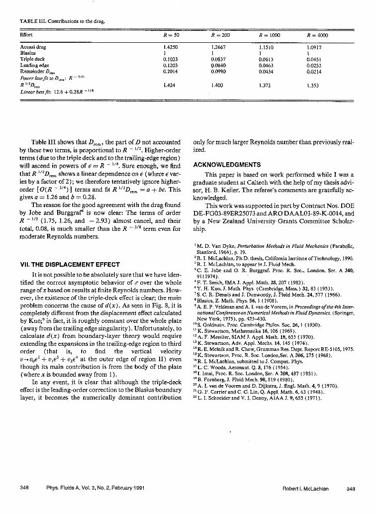
TABLE III. Contributions to the drag,

Effect

Actual drag Blasius Triple deck Leading edge Remainder D,, Power IawJit to D,, : R - ‘.” R ““D rem Linear bestfit: 12.6 4 0.28R -‘I’

R=50' R =200 R=1000 R=4OOO

1.4250 1.2667 1.1510 1.0917 1 1 1 1 0.1033 0.0837 0.0613 0.0451 0.1203 0.0840 0.0463 0.0252 0.2014 0.0990 0.0434 0.0214

1.424 l+%O 1.372 1.353

Table III shows that D,, , the part of D not accounted by these two terms, is proportional to R - 1’2. Higher-order terms (due to the triple deck and to the trailing-edge region ) will ascend in powers of E = R - 1’8. Sure enough, we find that R “‘D rem shows a linear dependence on E (where E varies by a factor of 2) ; we therefore tentatively ignore higher- order [O(R - 3’4) ] terms and fit R “2Drem = a + be. This gives a = 1.26 and b = 0.28.

The reason for the good agreement with the drag found by Jobe and Burggraf’ is now clear: The terms of order R -“* (1.75, 1.26, and - 2.93) almost cancel, and their total, 0.08, is much smaller than the R - 3/8 term even for moderate Reynolds numbers.

VII. THE DISPLACEMENT EFFECT

It is not possible to be absolutely sure that we have iden- tified the correct asymptotic behavior of r over the whole range ofx based on results at finite Reynolds numbers. How- ever, the existence of the triple-deck effect is clear; the main problem concerns the cause of d(x). As seen in Fig. 8, it is completely different from the displacement effect calculated by KLIO;~ in fact, it is roughly constant over the whole plate (away from the trailing edge singularity). Unfortunately, to calculate d(x) from boundary-layer theory would require extending the expansions in the trailing-edge region to third order (that is, to find the vertical velocity u+v,E2 + u,E3 + u2e4 at the outer edge of region II) even though its main contribution is from the body of the plate (where x is bounded away from 1) .

In any event, it is clear that although the triple-deck effect is the leading-order correction to the Blasius boundary layer, it becomes the numerically dominant contribution

only for much larger Reynolds number than previously real- ized.

ACKNOWLEDGMENTS

This paper is based on work performed while I was a graduate student at Caltech with the help of my thesis advi- sor, I-I. B. Keller, The referee’s comments are gratefully ac- knowledged.

This work was supported in part by Contract Nos. DOE DE-FG03-89ER25073 and AR0 DAAL03-89-K-0014, and by a New Zealand University Grants Committee Scholar- ship.

’ M. D. Van Dyke, Perturbation Methods in Fluid Mechanics (Parabolic, Stanford, 1964), p. 39,

‘R, I. McLachlan, Ph.D. thesis, California Institute ofTechnology, 1990. 3R. I. McLachlan, to appear in J. Fluid Mech. 4C!. E. Jobe and 0. R. Burggraf. Proc. R. Sot., London, Ser. A 340,

91( 1974). 5 F. T. Smith, IMA 3. Appl. Math. 28,209 ( 1982). &Y. Ii. Kuo, J. Math. Phys. (Cambridge, Mass.) 32,83 (1953). ‘S. C. R, Dennis and J, Dunwoody, J. Fluid Mech. 24,599 ( 1966). a Blasius, Z. Math. Phys. 56,l ( 1908). 9A. E. P. Veldman and A. I. van de Vooren, in Proceedings of the 4th Inter-

lrational Conferenceon Numericatkfethodsin FluidDynamics, (Springer, New York, 1995). pp. 423-430.

‘OS. Goldstein, Proc. Cambridge Philos. Sot. 26, 1 (1930). ” K. Stewartson, Mathematika 16, 106 (1969). "A, F. Messiter, SIAM 3. Appl. Math. 18,655 (1970). “K. Stewartson, Adv. Appl. Mechs. 14, 145 (1994). I4 R. E, Melnik and R. Chow, Grumman Res. Dept. Report RE-5 105,1975. “K. Stewartson, Proc. R. Sot. London,Ser, A 306,275 ( 1968). “R. I. McLachlan, submitted to J. Comput. Phys. “L. C. Woods, Aeronaut. Q. 5, 176 ( 1954). ‘*I. Imai, Proc. R. Sot. London, Ser. A 208,487 ( 1951). 19B. Fomberg, J, Fluid Mech. 98,819 (1980). *‘A. 1. van de Yooren and D. Dijkstra, J. Engl. Math. 4, 9 ( 1990). *’ G. F. Carrier and C. C. tin, Q. Appl. Math. 6.63 ( 1948). “L. I. Schneider and V. I, Denny, AIAA J. 9,655 (1991).

348 Phys. FluidsA,Vol.3,No.2,February199i Robertl.McLachlan 348

Physics of Fluids is copyrighted by the American Institute of Physics (AIP). Redistribution of journal material

is subject to the AIP online journal license and/or AIP copyright. For more information, see

http://ojps.aip.org/phf/phfcr.jsp

Documents

The boundary layer on a finite flat plate - Massey Universityrmclachl/PFA91.pdf · The boundary layer on a finite flat plate Robert I. McLachlan*) Appiied Mathematics, ... boundary-layer