Embed Size (px)
Citation preview

Gila Bronshtein Cornerstone Research
Jason Scott
John B. Shoven Stanford University and NBER
Sita N. Slavov George Mason University and NBER
January, 2018
Working Paper No. 17-047
The Power of Working Longer

1
The Power of Working Longer1
Gila Bronshtein
Cornerstone Research
Jason Scott
John B. Shoven
Stanford University and NBER
Sita N. Slavov
George Mason University and NBER
January 2018
Abstract
This paper compares the relative strengths of working longer vs. saving more in terms of
increasing a household’s affordable, sustainable standard of living in retirement. Both stylized
households and actual households from the Health and Retirement Study are examined. We
assume that workers commence Social Security benefits when they retire. The basic result is
that delaying retirement by 3-6 months has the same impact on the retirement standard of
living as saving an additional one-percentage point of labor earnings for 30 years. The relative
power of saving more is even lower if the decision to increase saving is made later in the work
life. For instance, increasing retirement saving by one percentage point ten years before
retirement has the same impact on the sustainable retirement standard of living as working a
single month longer. The calculations of the relative power of working longer and saving more
are done for a wide range of realized rates of returns on saving, for households with different
income levels, and for singles as well as married couples. The results are quite invariant to these
circumstances.
JEL codes: H55, D14, J26
1 This research was supported by the Alfred P. Sloan Foundation through grant #G-2017-9695. The views and
approaches in this paper are solely those of the authors and do not represent the views of Cornerstone Research,
Stanford University, George Mason University or the NBER. The authors are grateful to Ben Kaufman for
outstanding research assistance.

2
1. Introduction
One of the biggest financial challenges people face is allocating lifetime resources in such
a way as to support a satisfactory and sustainable standard of living in retirement. Households can
explicitly or implicitly establish a plan at a relatively early age, but there is a great deal of
uncertainty about important factors such as future wage growth, asset returns, life expectancies,
annuity prices and Social Security benefit formulas at the time of retirement. The key decisions to
make include when to start saving for retirement, what percentage of earnings to contribute to
employer-based tax deferred saving accounts, what asset returns and expenses to assume, and at
what age to retire. As time passes and some of this uncertainty is resolved, households should
reassess their strategy for providing resources for retirement. For example, households today may
wish to re-optimize retirement strategy in light of persistently low real interest rates and wage
growth. In a standard life cycle model with uncertainty, households continually reassess and
reoptimize as new information is revealed. In reality, households facing constraints on their time
and attention could reexamine their plan at periodic intervals, such as every ten years.
In this paper, we examine how households that are close to retirement could reassess
retirement plans. Rather than specifying a full-blown life cycle model, we examine the marginal
impact of saving and retirement choices on sustainable retirement consumption. This framework
allows us to see how each of these margins influences retirement consumption, thereby defining
the tradeoffs that households face. The optimal choice with respect to these tradeoffs will of course
depend on household preferences. But spelling out the tradeoffs can provide practical guidance for
individuals and financial planners. We calculate the impact of working longer on retirement
consumption and compare it to the impact of saving more or switching to assets with lower expense
ratios. We examine this issue for both stylized households and actual households from the Health

3
and Retirement Study (HRS), a nationally representative panel of older adults. Our key insight is
that some decisions, such as how much to save in retirement accounts going forward, become less
powerful at older ages in changing the affordable retirement standard of living. Saving an
additional one percent of earnings, for instance, would affect the retirement standard of living
much more at age 36 than at age 56. Similarly, the impact of choosing cost-efficient assets –
something financial planners frequently emphasize to increase retirement resources – diminishes
with age since there are fewer years to enjoy the benefit of a lower cost portfolio. In contrast,
changes to planned retirement and Social Security claiming dates continue to have the same impact
on retirement living standards as a person ages.
We define the maximum sustainable standard of living in retirement as the maximum
annuity that can be obtained from both private retirement savings and Social Security. We assume
that retirement accumulations are used to purchase an inflation-indexed joint survivor life annuity
with 100% of the monthly benefit continuing for the survivor. Annuitizing wealth guarantees that
the benefits are indeed sustainable and protected from both inflation and the risk of outliving
retirement resources, and is generally optimal in the life cycle framework (see Yaari 1965; Mitchell
et al. 1999). It also facilitates our analysis by ensuring that the annuity benefits from 401(k) and
similar plans are comparable to Social Security benefits for primary earners, where the benefits
are paid out as a second-to-die inflation-indexed annuity. We assume that workers claim Social
Security upon retirement, and therefore workers who extend their careers postpone the
commencement of Social Security to their new retirement age. Claiming Social Security upon
retirement is not necessarily optimal. In fact, most primary earners benefit from delaying Social
Security to age 70 regardless of retirement age2, and using private retirement assets to finance a
2 See, e.g., Meyer and Reichenstein (2010); Munnell and Soto (2005); Sass, Sun, and Webb (2007, 2013); Coile et
al. (2002); Mahaney and Carlson (2007); Shoven and Slavov (2014a, b).

4
delay of Social Security is superior to annuitizing them (Bronshtein et al. 2017). However,
claiming Social Security upon retirement matches actual behavior of most Americans and appears
to be a social norm (Shoven, Slavov, and Wise 2017). We further assume that individuals who
continue to work continue to contribute to their employer’s defined contribution plan. We show
that postponing retirement impacts the sustainable standard of living in retirement for several
reasons: (1) commencing Social Security at a later age results in higher monthly benefits, (2)
working longer involves additional contributions to retirement accounts, (3) delayed withdrawals
from retirement accounts results in additional compounding of previous account balances, and (4)
delayed annuity purchase results in lower annuity prices (that is, a given amount of wealth will
convert to a larger monthly annuity payment).
The stylized analysis and the empirical results from the HRS lead to the same conclusion.
Working longer is a powerful method to increase retirement standard of living and has a
substantially larger impact on retirement consumption than other alternatives, particularly in mid-
and late-career circumstances. For individuals who are 30 years away from retirement, extending
work for six months or less has the same impact as increasing annual retirement contributions by
one percentage point. For near retirees, increasing retirement contributions has even less relative
strength. In those cases, a one-percentage point increase in the contribution rate may be equivalent
to postponing retirement by a single month. While the optimal choice depends on household
preferences, including the disutility of work, these are the tradeoffs. Our analysis provides valuable
information to households as they consider the levers that they have at their disposal to increase
their retirement standard of living.

5
2. Analysis of Stylized Households
The traditional economic approach to modeling saving and retirement decisions is based
on the life cycle model. In a standard life cycle model, households aim to smooth consumption
over the lifetime by saving during working years and drawing down on savings during retirement
years (Friedman 1957; Modigliani 1966). Life cycle models can incorporate uncertainty in a range
of outcomes, such as wages, asset returns, and health. Some studies have introduced endogenous
retirement into the life cycle model by having the marginal cost of effort increase or the marginal
value of leisure decrease with age (e.g., Gustman and Steinmeier 1986; Blau 2008). Some studies
have explored the implications of various policy changes, such as an increase in the pension
eligibility age on retirement (Haan and Prowse 2014). A few papers have used the life cycle
framework to examine the impact of the actuarial adjustment for delaying Social Security on
consumption and retirement behavior (e.g., Gustman and Steinmeier 2008; 2015). For example,
Gustman and Steinmeier (2008) predict that changes to Social Security rules between 1992 and
2004, including the increase in the delayed retirement credit, increased the male labor force
participation rate.
While the standard life cycle model provides the theoretical framework for our approach,
we focus directly on the marginal impact that adjusting saving and retirement decisions has on the
maximum sustainable consumption in retirement. This allows us to examine the tradeoffs that
households approaching retirement face. Like Gustman and Steinmeier (2008; 2015), we show
that the recent, more generous rules for delaying Social Security play a large role in the returns to
working longer relative to saving more, although other factors matter too.
We begin by analyzing stylized workers who have smoothly growing wages and constant
asset returns, and who participate in the labor force without interruption. The advantage of

6
examining stylized workers is that the underlying arithmetic relationships between saving, wealth
accumulation, and annuitization are readily transparent. Analyzing such individuals will give us
guidance on what to expect from real households with more complicated financial lives. We start
with an equation for the evolution of wealth in a defined contribution retirement plan as a function
of previous contributions and returns:
𝑊𝑇 = ∑ {𝐶𝑡 ∏ (1 + 𝑟𝑖)
𝑇
𝑖=𝑡+1
} + 𝐶𝑇
𝑇−1
𝑡=1
In this equation, 𝑊𝑇 is wealth at time 𝑇, 𝐶𝑡 is annual contribution made at time 𝑡, and 𝑟𝑡 is the
return over the period (𝑡 − 1, 𝑡). The above equation has the household starting retirement saving
at time 0 and shows wealth accumulation as a function of time 𝑇. The equation assumes that
contributions take place at the end of each year of work, so that the final contribution does not earn
any asset returns. This annual version of the accumulation equation is sufficiently accurate for our
stylized examples, but it should be clear that a monthly version with monthly asset returns would
be simple to implement.
In our stylized examples, we assume that workers earn the same real wage, 𝜔, in each
period of life. We further assume that there is no economy-wide wage growth. Social Security
benefits are based on Average Indexed Monthly Earnings (AIME), calculated as the average of the
highest 35 years of earnings, indexed for economy-wide wage growth and divided by 12 to convert
to a monthly amount. Workers who claim at full retirement age (FRA) receive a monthly benefit
(called the primary insurance amount, or PIA) equal to 90 percent of the first $885 of AIME, 32
percent of any AIME between $885 and $5,336, and 15 percent of any remaining AIME.3 Our
3 These PIA “bend points” are in effect for 2017. In general, bend points are indexed to average age growth. To
calculate AIME, wages are indexed to the year in which the worker turns 62 (with any additional years of earnings
counting at their nominal value), and PIA is based on the bend points in effect during the year in which the worker

7
assumption of zero real wage growth, both for the individual worker and economy-wide, implies
that AIME is equal to the monthly equivalent of 𝜔. For our stylized worker, we assume that the
ratio of PIA to AIME is equal to 0.42. That value is roughly in line with the ratio for a worker who
earns the economy-wide average wage in each year of his or her career.4 Due to the progressivity
of the PIA formula, the ratio of PIA to AIME declines with AIME. This fact will become relevant
later when we consider workers with different levels of earnings.
At the time of retirement, the household annuitizes the accumulated wealth and commences
Social Security benefits. We define the retirement replacement ratio as the sum of the annuity
payments and Social Security benefits divided by pre-retirement income. Specifically, the
retirement replacement ratio, if retirement occurs at time 𝑇, is:
𝜌𝑇 = 𝐴𝑇 ∙ 𝑊𝑇 + 𝑆𝑇
𝜔
where 𝐴𝑇 is the annual annuity conversion factor relevant at time 𝑇, 𝑆𝑇 is the annual Social
Security benefit at time 𝑇, and 𝜔 is the annual wage. The annuity conversion factor, 𝐴𝑇, converts
retirement wealth into the annualized inflation-indexed life annuity benefit. Recent quotes for
annuity factors for same-age married couples and single men and women are shown in Figure 1.
turns 62. PIA is indexed for price inflation after age 62. For our stylized example, since we have assumed zero wage
growth, we are simply using the bend points for 2017. 4 See Table V.C7 of the Social Security Trustees Report for 2013, at
https://www.ssa.gov/oact/tr/2013/V_C_prog.html#997444. This table reports the ratio of PIA to career-average
indexed earnings (similar to AIME) for individuals whose career-average earnings are equal to the economy-wide
wage index. The average of these ratios for workers reaching full retirement age in 2013, 2015, and 2020 is roughly
42 percent. The Trustees Reports stopped reporting these ratios in 2014.

8
Source: Conversion factors are based on CPI-adjusted single life and 100% Joint and Survivor
annuity quotes for from Immediate Annuities retrieved on August 9th, 2017, and authors’
calculations.
The lowest curve shows the annuity conversion factors for same-age married couples and the
highest curve shows the factors for single men. These quotes reflect several important realities.
First, increasing sustainable lifetime standard of living is very expensive. At age 62, the conversion
factor for couples is .033267, which means that an additional $100,000 of retirement wealth would
raise the annual inflation-adjusted standard of living by just $3,327 per year. These quotes
implicitly take into account the current low real interest rates and the anticipated mortality of
today’s retirement age individuals.
0
0.01
0.02
0.03
0.04
0.05
0.06
62 63 64 65 66 67 68 69 70
Figure 1: Annuity Conversion Factors for Same-Age Couples, Single Women and Single Men
Couple Male Female

9
Financial planners often use replacement ratios like the one above to summarize a
household’s goal for a sustainable retirement living standard. These ratios are a rule of thumb
deriving from the life cycle framework. Scholz and Seshadri (2009) show that optimal replacement
rates derived from a life cycle model vary greatly by household; for example, a couple with
children should target a lower replacement rate than a couple without children as the former can
reduce child care expenses during retirement. In addition, there has been some debate regarding
the appropriate denominator.5 Numerous alternatives are possible, such as final salary, real average
salary over the lifetime, AIME, or real average salary over the 5 years prior to retirement. The
optimal replacement ratio can vary greatly depending on the choice of denominator. In our stylized
examples, since we assume zero wage growth both economy wide and for the individual, all these
denominator choices are equivalent. Moreover, we do not take a stand on the optimal replacement
ratio. Instead, we examine how changes in saving and retirement decisions affect retirement living
standards at the margin. Using replacement ratios to summarize retirement living standards
simplifies the presentation of our stylized examples. However, even with wage growth, our results
would be insensitive to the choice of denominator or to other factors that influence the optimal
replacement rate. As long as the replacement ratio denominator is held constant, the growth rate
in the replacement ratio will be equal to the growth rate in retirement income.
Next, we list our base case assumptions, summarized in Table 1. We start by looking at the
primary earner in a same-age couple, who chooses to start saving at age 36. This is 𝑡 = 0 in the
wealth accumulation equation. Their employer offers to match 50% of employee contributions to
a 401(k) plan, up to 6 percent of salary. The worker assumes that he or she will have this plan or
an identical plan available to them for their entire career. The worker’s initial plan is to work until
5 See Biggs (2008, 2016) for further discussion.

10
age 66, then retire, annuitize any 401(k) account balances, and commence Social Security benefits.
The worker intends to take advantage of the employer’s match offer and contribute 6 percent to
the retirement plan, with the employer matching with an additional 3 percent. In addition to zero
wage growth, we assume a constant return on assets (zero percent in the base case, though we
consider alternatives). Our assumptions about wage growth and asset returns are not far out of line
with recent experience. Real median wages have been quite stagnant for several decades and safe,
real asset returns such as interest rates on Treasury Inflation Protected Securities (TIPS) have been
roughly zero for the past nine years.
Table 1: Baseline Assumptions
Assumption Value
Constant real wage 𝜔
Contributions are 9% of salary (e.g. 6% employee / 3%
employer) 𝐶𝑡 = 0.9 ⋅ 𝜔
Constant real returns, 𝑟, assumed to be zero 𝑟1 = 𝑟2 =. . = 𝑟𝑇 = 𝑟 = 0
30 year saving horizon, starting at age 36 and retirement age 66 𝑇 = 30
PIA is 42% of AIME (equal to constant wage) 𝑆𝑇/𝜔 = 0.42
Annuity conversion factor at age 66 𝐴𝑇 = .03748125
Annuity conversion factor at age 67 𝐴𝑇 = .03871467
With these assumptions, we have the following base case replacement ratio:
𝜌𝑇 = 𝐴𝑇∙𝑊𝑇
𝜔+
𝑆𝑇
𝜔=
𝐴𝑇∙30∙.09𝜔
𝜔+
𝑆𝑇
𝜔= .1011994 + .42 = .5211994
Despite 30 years of saving 9 percent of earnings, the annuitized 401(k) balance accounts for only
19.4 percent of retirement income with Social Security accounting for the remainder. This fact
alone highlights the incredible value of Social Security benefits for primary earners.

11
2.1 Working an Additional Year at Age 66.
If our stylized primary earner delays retirement by one year to age 67, there are four main
impacts on retirement income:
1. The annuity is cheaper (i.e., each dollar of savings will convert to a larger annuity
payment) - the new conversion factor would increase to 𝐴𝑇+1 = .03871467.
2. Wealth increases by the return on assets (initially ignored since asset returns are
assumed to be zero).
3. Wealth increases by the additional retirement contribution, 𝑊𝑇+1 = 𝑊𝑇 + 𝐶𝑇.
4. The Social Security monthly benefit increases by 8% over and above inflation.
The replacement ratio at age 67 is then:
𝜌𝑇+1 = 𝐴𝑇+1 ∙ 𝑊𝑇+1
𝜔+
𝑆𝑇+1
𝜔=
𝐴𝑇+1 ∙ 31 ∙ .09𝜔
𝜔+
1.08 ⋅ 𝑆𝑇
𝜔= .1080139 + .4536 = .561614
By working one year longer, the replacement rate has increased from around 52.1 percent to 56.2
percent. Recall that as long as the denominator used in the replacement rate is held constant, the
growth in the replacement rate is mathematically equal to the growth in retirement income, so we
can conclude that by working one year longer retirement income has increased by 7.75 percent.
This increase is a weighted average of the 8 percent increase in real Social Security benefits and
the 6.73 percent increase in the real value of the annuity payment obtained from the 401(k) balance
at retirement. The weights are based on the share of each of the elements in the replacement ratio
at the initial planned retirement age (about 81% and 19%, respectively). Even with zero percent
returns, the annuity payment still increases due to the additional contributions for one year and due
to the fact that annuities are cheaper at 67 than at 66. This example emphasizes that the returns to
working longer can be quite high even when asset returns are low.
12
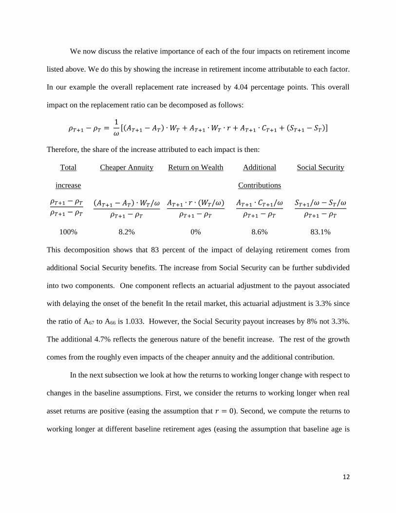
We now discuss the relative importance of each of the four impacts on retirement income
listed above. We do this by showing the increase in retirement income attributable to each factor.
In our example the overall replacement rate increased by 4.04 percentage points. This overall
impact on the replacement ratio can be decomposed as follows:
𝜌𝑇+1 − 𝜌𝑇 = 1
𝜔[(𝐴𝑇+1 − 𝐴𝑇) ∙ 𝑊𝑇 + 𝐴𝑇+1 ∙ 𝑊𝑇 ∙ 𝑟 + 𝐴𝑇+1 ∙ 𝐶𝑇+1 + (𝑆𝑇+1 − 𝑆𝑇)]
Therefore, the share of the increase attributed to each impact is then:
Total
increase
Cheaper Annuity Return on Wealth Additional
Contributions
Social Security
𝜌𝑇+1 − 𝜌𝑇
𝜌𝑇+1 − 𝜌𝑇
(𝐴𝑇+1 − 𝐴𝑇) ∙ 𝑊𝑇/𝜔
𝜌𝑇+1 − 𝜌𝑇
𝐴𝑇+1 ∙ 𝑟 ∙ (𝑊𝑇/𝜔)
𝜌𝑇+1 − 𝜌𝑇
𝐴𝑇+1 ∙ 𝐶𝑇+1/𝜔
𝜌𝑇+1 − 𝜌𝑇
𝑆𝑇+1/𝜔 − 𝑆𝑇/𝜔
𝜌𝑇+1 − 𝜌𝑇
100% 8.2% 0% 8.6% 83.1%
This decomposition shows that 83 percent of the impact of delaying retirement comes from
additional Social Security benefits. The increase from Social Security can be further subdivided
into two components. One component reflects an actuarial adjustment to the payout associated
with delaying the onset of the benefit In the retail market, this actuarial adjustment is 3.3% since
the ratio of A67 to A66 is 1.033. However, the Social Security payout increases by 8% not 3.3%.
The additional 4.7% reflects the generous nature of the benefit increase. The rest of the growth
comes from the roughly even impacts of the cheaper annuity and the additional contribution.
In the next subsection we look at how the returns to working longer change with respect to
changes in the baseline assumptions. First, we consider the returns to working longer when real
asset returns are positive (easing the assumption that 𝑟 = 0). Second, we compute the returns to
working longer at different baseline retirement ages (easing the assumption that baseline age is

13
66). Third, we calculate the returns to working more than one year longer. Fourth, we consider the
impact of working longer for different wage levels. Last, we estimate the returns for singles.
2.2 Role of Real Investment Returns
We consider real investment returns ranging from 0% to 8%. The second column of Table
2 reports the growth in retirement income relative to the baseline as a result of one additional year
of work. The results suggest that the relative impact of working longer is fairly insensitive to asset
returns; one additional year of work raises retirement income by roughly 8 percent for real returns
of 0-3% and then the income increase gradually rises to about 10 percent in the case of 8%
compounded real returns.
Table 2 - Returns to Working Longer by Real Investment Returns
Shares in the Retirement Income Growth
Investmen
t Returns
Retirement
Income Growth
(%)
Cheape
r
Annuit
y
Return
on
Wealth
Additional
Contributio
n
Social
Securit
y
0% 7.75% 8.2% 0.0% 8.6% 83.1%
1% 7.85% 9.2% 2.9% 8.3% 79.7%
2% 7.98% 10.1% 6.4% 7.8% 75.7%
3% 8.15% 11.2% 10.5% 7.4% 71.0%
4% 8.39% 12.2% 15.3% 6.8% 65.7%
5% 8.70% 13.2% 20.7% 6.2% 60.0%
6% 9.09% 14.1% 26.5% 5.6% 53.9%
7% 9.56% 14.9% 32.6% 4.9% 47.6%
8% 10.13% 15.5% 38.9% 4.3% 41.4%
In the last four columns of Table 2 we present the share of the increased retirement income
attributable to each of the four impacts described above. The growth rate of the Social Security
benefit is constant across the investment returns but its share in total retirement income growth
decreases from 83% as asset returns increase. Similarly, the effect of the additional contribution is
14
constant across the investment returns, so that its share in the total increase diminishes as returns
increase. However, the impact of the additional return on existing wealth and the cheaper annuity
are larger at higher investment return rates. Therefore, their share in the total retirement income
increases. However, even when asset returns are very high (7-8%), the impact of Social Security
still dominates the increase in retirement income.
Throughout, we assume that annuity prices are invariant to asset returns. That is, we use
the same annuity factors, based on current conditions, in all calculations regardless of asset returns.
It is possible that higher investment returns may be associated with higher discount rates and
therefore lower annuity prices. However, high investment returns do not necessarily imply low
annuity prices. Annuity prices are mainly based on risk-free interest rates. Over the last several
years, investment returns have been high while safe interest rates (such as those on inflation-
indexed government bonds) have remained low, a discrepancy that may be attributable to a higher
risk premium. Alternatively, the higher investment returns we have considered in this section can
be thought of as ex-post returns on potentially risky investments.
2.3 Varying Age and Length of Extension
So far, we have been looking at the power of working to 67 vs. a base case of retiring at
66. But many people retire well before age 66. So, how powerful is working an extra year at age
62 or 63? And what is the impact of delaying retirement by longer than one year? To estimate the
returns to working longer at different ages and for different work extension lengths, we return to
our baseline case: a primary earner in a same-age married couple who started at age 36 to
contribute 9 percent of salary to a defined contribution retirement plan. Asset returns and wage
growth are equal to zero. There are two key differences in this exercise compared to our base case.

15
First, the number of years of saving changes. Clearly, retiring before age 66 means fewer years of
accumulated saving (relative to our base case) and retiring after age 66 means greater years of
accumulated savings (relative to our base case). Second, the Social Security benefit changes since
Social Security pays 100% of PIA for those claiming benefits at the full retirement age (which is
66 for those born between 1943 and 1954) but substantially lower benefits for those claiming
earlier and substantially higher for those claiming after their full retirement age.6
The first column of Table 3 presents the percent increase in retirement income resulting
from working one year longer and delaying the claiming of Social Security by one year for primary
earners of age 62 through 69. By age 70 Social Security benefits no longer grow through delay,
and the returns to working longer are much lower. There are a few notable results. First, as a result
of the peculiar structure of the Social Security benefits, returns to working longer are non-linear.
Delaying from age 62 to 63 increases retirement income by 6.7%. Returns are the highest for those
aged 63 (about 8%), lower for those aged 64 and 65, and increase again to 7.75% for those aged
66. The rest of Table 3 displays the percentage increase in retirement income for those choosing
to delay by two through eight years, up to age 70. The returns are relative to the age displayed in
the first column of Table 3. For example, delaying by 4 years at age 64 (i.e., through age 68)
increases retirement income by 33.04 percent.
6 For those born between 1943 and 1954, the Social Security monthly benefit is reduced by 5/9ths of one percent of
PIA for each month between 1 and 36 months prior to full retirement age that the benefit is claimed, and 5/12ths of
one percent of PIA for each additional month prior to full retirement age that the benefit is claimed. For example,
claiming at age 62 will reduce the Social Security benefit to be 75% of PIA, claiming at age 63 will reduce the
benefit to 80% of PIA, and so on. For claims after full retirement age, the monthly benefit increases by 2/3rds of one
percent of PIA per month of delay up to 48 months. For example, delaying to age 70 increases the benefit to 132
percent of PIA.

16
Table 3: Returns to Working Longer by Age and Length of Extension
Base Number of Working Years Extensions
Age 1 year 2 years 3 years 4 years 5 years 6 years 7 years 8 years
62 6.70% 15.27% 23.92% 32.67% 42.96% 53.36% 63.89% 74.57%
63 8.03% 16.13% 24.34% 33.98% 43.73% 53.60% 63.60% 64 7.50% 15.10% 24.02% 33.04% 42.18% 51.44% 65 7.07% 15.36% 23.76% 32.26% 40.88% 66 7.75% 15.59% 23.53% 31.58% 67 7.28% 14.64% 22.11% 68 6.87% 13.83% 69 6.51%
The results are unequivocal. Primary earners of ages 62 to 69 can substantially increase their
retirement standard of living by working longer. The longer work can be sustained, the higher the
retirement standard of living. For example, retiring at 66 instead of 62 increases retirement living
standard by about one-third. As we will show in the Section 3, no reasonable amount of additional
saving could impact the retirement standard of living so significantly.
2.4 Returns to Working Longer by Different Earnings Levels
The previous analysis assumed a stylized worker with roughly average earnings (which
translated into a PIA to AIME ratio of 42 percent). However, as we noted earlier, the PIA formula
is progressive, so the ratio of PIA to AIME falls as AIME rises. For the following exercise, we
consider five different levels of the PIA to AIME ratio, as shown in the first column of Table 4.
These PIA to AIME ratios translate into the annualized AIME levels shown in the second column
of Table 4. If we continue to assume zero wage growth, both economy-wide and for individual
workers, then this annualized AIME is equal to the wage earned in each year of work.7 We then
7 In reality, AIME may not translate one-for-one into annual earnings, as AIME is based on the top 35 years of
indexed earnings. For example, a person with a short career and high annual earnings may have the same AIME as a

17
calculate the returns to working one year longer for the five earning levels. We continue to assume
a primary earner in a couple aged 66, saving 9% of salary for 30 years with zero percent real asset
returns.
In the third column of Table 4 we present the returns to working longer in terms of
percentage increase in retirement income. These results indicate that the returns to working longer
– expressed as the percentage increase in retirement income – are about the same across the income
levels (about 7.75%, as our baseline results). However, the impact of working longer on the
replacement rate varies significantly across the different wage levels. A growth rate of 8% has
roughly three times the impact on the replacement rate assuming a base replacement rate of 75%
compared to a base replacement rate of 25%.
The second result observed in the table is that the returns to working longer decrease as
earnings increase. A decomposition of the four impacts (not presented) reveals that the first three
impacts – cheaper annuity, returns to wealth and additional contribution – are constant across wage
levels. However, the Social Security impact changes. As the Social Security share of final
retirement income increases, the weight on the Social Security impact increases. Thus, an 8%
growth in the Social Security benefit has a higher weight for workers at the lower wage levels,
translating into higher returns to working an additional year.
Table 4 - Returns to Working Longer by Income Level
PIA/AIME AIME (annual
wage) Income Retirement
Growth (%)
70% 16,212 7.84%
60% 21,996 7.82%
50% 34,224 7.79%
40% 68,184 7.74%
30% 113,628 7.68%
person with a long career and low annual earnings. In our stylized examples, individuals are assumed to work full
careers.

18
2.5 Single Individuals
All of the above analysis was for the primary earner of a couple. In that case, Social
Security benefits are paid in the form of a second-to-die annuity, and we assume private retirement
wealth is converted into the same form. We now address how working longer impacts retirement
living standard for single individuals. While the increase in Social Security is the same as our base
case, the annuity factors are different. For singles, the analysis is identical for men and women
except that retail annuities are cheaper for men due to their shorter life expectancy. (For married
primary earners, the gender of the primary earner did not matter. A 100 percent joint and survivor
annuity is priced based on one male and one female lifetime.) Of course, annuities are cheaper for
both single men and women compared to primary earners, since primary earners buy a second-to-
die annuity and singles buy single life annuities.
The returns to working one additional year at age 66 for single males, single females, and
married primary earners are shown in Figure 2. We illustrate in this graph how the returns increase
as we ease the assumption of zero rate of returns on assets. Returns are slightly higher for single
males, and to a lesser degree for single females, compared to married primary earners. These small
differences are driven by the impact of working longer on annuity prices (resulting from delaying
the annuity purchase by one year). It is important to note, however, that these figures represent the
increase in annual retirement income rather than lifetime retirement income. The increase in
lifetime retirement income is always greater for married couples compared to singles, as the higher
income is paid out as a second-to-die annuity rather than a single life annuity (see e.g., Shoven and
Slavov 2014a,b).

19
3 Working Longer vs. Alternative Strategies
3.1 Alternative Strategy: Save One Percent More of Earnings
An alternative way to boost retirement living standards is to save more. Suppose that our
stylized primary earner saves 1 percent more of wages starting at age 36. That is, they move from
a 6 percent to a 7 percent personal contribution rate, with a 3 percent employer contribution, for a
total retirement saving rate of 10 percent. If the higher contribution rate were applied for the entire
30 years (maintaining the assumption of zero real asset returns and wage growth during those 30
0
2
4
6
8
10
12
0 1 2 3 4 5 6 7 8
Real Assets Rate of Return
Figure 2: Percentage Increase in Retirement Income from One Additional Year of Work at age 66
by Marital Status and Real Asset Rate of Return
Couples Men Women

20
years), then the replacement rate would rise to .53244 from the base case of .521194, translating
into a 2.16% percent increase in retirement income.8
Recall from Section 2.1 that working one year longer increased retirement income by
7.75%. Delaying retirement by one year is roughly 3.5 times as impactful as saving an additional
1 percent of wages for 30 years. To put it another way, working just over 3 months longer would
have the same impact as a 1 percentage point increase in the contribution rate for 30 years. In what
follows we compare various alternatives that would increase retirement income to the working
longer alternative. For all these cases, we state the number of additional working months required
to have an equal impact on retirement income. The message resulting from this comparison is
clear. Working longer is very powerful compared to the other alternatives. This result holds for all
reasonable investment returns and ages considered.
3.2 Role of Real Investment Returns
In Section 2.2 we considered the effect of various asset returns on returns to working one
year longer. In Table 5 below we demonstrate how the returns to saving 1% more of wages for 30
years change with respect to the real asset returns.9 As expected, saving has a larger impact on
retirement income when real asset returns are higher. However, the returns to saving more are
much smaller than the returns to working one year longer shown in Table 2. For low asset returns,
working 3-4 months longer increases retirement income about the same as increasing the
contribution rate by 1 percentage point more for 30 years. At high asset return levels, working
8 Recall that since we are keeping the denominator in the replacement rate calculation constant, the growth in the
replacement rate is equal to the growth in retirement income. 9 As in section 2.2, we assume annuity prices do not change as investment returns increase.

21
around half a year longer has the same impact as increasing the contribution rate by 1 percentage
point.
Table 5 - Returns to Saving 1% More of Earnings by Real Investment Returns
Investment
Returns
Retirement
Income Growth
(%)
Number of additional months of work
equal to 1% additional saving for 30
years
0% 2.16% 3.3
1% 2.43% 3.7
2% 2.73% 4.1
3% 3.07% 4.5
4% 3.45% 4.9
5% 3.87% 5.3
6% 4.32% 5.7
7% 4.79% 6.0
8% 5.29% 6.3
3.3 Role of Start Age
Now, let us look at different start ages for saving 1% more of wages. The base case is still
a contribution rate of 9 percent starting at age 36. We examine three alternatives (increasing the
contribution rate by 1 percentage point at ages 36, 46 and 56) and compare the impact of these
three scenarios with never increasing the contribution rate but working one year longer. Table 6
contains the results for two investment returns, zero and five percent.
Table 6 - Returns to Saving 1% More of Earnings, by Age Initiated
Age Investment
Returns
Retirement
Income Growth
(%)
Number of additional months of work
equal to 1% additional saving for 30
years
36 0% 2.16% 3.3
36 5% 3.87% 5.3
46 0% 1.54% 2.4
46 5% 2.33% 3.2
56 0% 0.83% 1.3
56 5% 1.02% 1.4

22
The table shows that as the number of additional saving years decreases, the impact of the
asset return assumption diminishes. That is, the impact of a 5% real asset return has a much smaller
effect relative to a zero percent return when the contribution rate is increased for only 10 years.
Second, as reflected in the last column, at age 56, the power of saving one percent more of income
is equivalent to working just one additional month (regardless of the return environment
considered). That is, the older the individual, the greater the relative impact of working longer
compared to increasing the saving rate.
3.4 Role of Earnings Levels
As we have shown in Section 2.4, the impact of working longer on the growth rate in
retirement income is insensitive to income levels. In this section, we examine the impact of saving
an additional 1% on different income groups’ retirement living standards. In Table 7 we present
the returns to saving more for different income levels (as indicated by PIA/AIME ratios, which
correspond to annual earnings under the zero-wage growth assumption).
Table 7 - Saving More or Working Longer by Income Level
Annualized AIME
(Wage)
PIA/AIME
(Replacement Rate)
Months of work to equal 1% additional
saving for: 30 Years 20 Years 10 Years
$16,212 70% 2.1 1.4 0.7
$21,996 60% 2.5 1.6 0.8
$34,224 50% 2.9 1.9 1.0
$68,184 40% 3.5 2.3 1.2
$113,628 30% 4.4 2.9 1.5
In terms of replacement rate, we see that Social Security is highly progressive. At a wage
rate of $16,000, Social Security replaces 70% of income, whereas the replacement rate at $113,000

23
is only 30%. When Social Security replaces a larger fraction of income, working longer is
relatively more impactful than saving more. For example, compare a high wage worker to a low
wage worker each considering whether to save for 30 years or work longer. The lower wage
worker need only work 2.1 months to equal the benefit of 30 years of saving, whereas the higher
wage worker has to work more than twice as long, 4.4 months, to receive a comparable benefit.
The impact of saving more falls precipitously if saving occurs for fewer years. In this case, a low
wage worker saving more for 10 years need only work about 3 weeks to garner a comparable
benefit.
Consider this information in a more realistic setting. Suppose a high wage worker is 46
years old and is deciding between saving an additional 10% of salary for the next 20 years or
working longer. The alternative to saving an extra 10% for 20 years is to plan on working an extra
29 months.10 For the low wage worker, the decision would be between saving an additional 10%
for 20 years, or working an extra 14 months. If the low wage worker were 56, then the decision
would be between saving an additional 10% for 10 years or working a mere 7 months longer. The
disutility of work would have to be very high for low wage workers to consider saving more rather
than working longer.
3.5 Understanding the Results: Saving More vs. Working Longer
Clearly working one year longer is much more powerful than saving one percentage point
more for 30 years. But, why is working longer so much more powerful? The income and saving
that results from one more year of work is only a small part of the story. Our calculations show
that working longer is only powerful if accompanied by deferring the commencement of Social
10 Since the Social Security benefit growth varies over different ages, the calculation is not exact for horizons that extend beyond 12 months.

24
Security and the annuitization of the accumulated 401(k) balance. Recall that in our base case,
working one additional year to 67 – and simultaneously and deferring Social Security and the
annuitization of defined contribution balances – increased the sustainable real standard of living
for the couple’s retirement by 7.75 percent. That is a very big impact.
Now, consider another scenario, where the primary earner commences Social Security at
66, annuitizes his or her retirement assets at the same time, and then decides to work for another
year while making a 9 percent contribution to the company’s 401(k) plan. This is a case of working
longer with no deferrals at all, and the the sustainable standard of living would increase by only
0.67%.
This calculation illustrates that working longer only has a powerful impact on retirement
income if it facilitates delay of Social Security claiming and annuitization. Of course, Social
Security and annuitization can both be delayed without working longer. Alternatively, Social
Security can be delayed and 401(k) assets used to finance living expenses during the delay period.
But given the presence of liquidity constraints and the strong social norm of claiming Social
Security upon retirement, it is plausible that delaying retirement can facilitate delays in both
claiming Social Security and tapping into 401(k) wealth.
3.6 Alternative Strategy: Use More Cost-Efficient Portfolios
One of the key services provided by financial planners is helping clients reduce portfolio
costs. Lower portfolio costs translate into higher net asset returns and higher retirement income.
In our last exercise, we compare the impact of reducing portfolio management costs to the impact
of working longer. Overall, our results in this section suggest that the gains from choosing more
cost-efficient portfolios are relatively small compared to the gains from working longer. Thus,

25
financial planners may have more of an impact on clients’ retirement living standards by helping
them time their retirement (and Social Security claiming) optimally than by helping them choose
cost-efficient portfolios.
We return to the case of the primary earner in a couple who started contributing 9% of
earnings to a 401(k) at age 36, and planned to retire and collect Social Security at 66. The rates of
returns that have been used in the analysis up to now should be interpreted as net returns to
investors. We now look at the impact of increasing those returns by 60 basis points (0.6%), which
may be achieved by investing in lower cost mutual funds. Specifically, 60 basis points is roughly
the average difference between the expense charges of active and passive mutual funds, but it is
also possible to find active funds that are 60 basis points cheaper than some of the alternatives.
(There is little to no evidence that the more expensive funds have greater gross returns.)
Table 8 shows the impact of reducing portfolio costs at different levels of net investment
returns. Comparing these results to those in Tables 2 and 5, we can see that improving returns by
60 basis points for 30 years has about the same impact as saving one percentage point more for the
same duration. Both of these strategies have a much smaller impact than working an additional
year. The last column in Table 8 shows that to replicate the impact of cost efficient investments on
retirement income, a primary earner would need to work just under 3 months more in the low real
asset return environment and around 6 months more in a high return environment. Finally, if one
could use a two-pronged approach of reducing portfolio management costs by 60 basis points and
saving an additional 1% of earnings (both maintained for 30 years), the impact on retirement
income would be equivalent to that of working one year longer if asset returns are high. If this
combined strategy were implemented at age 56, just ten years before retirement, then the impact

26
on retirement income for an average earner would be equivalent to working three to four months
more.
Table 8 - Returns to Reducing Portfolio Costs
Original Net
Investment
Returns
Income Retirement
Growth (%)
Number of additional months
of work equal to 60 bp
reduction in expense ratio for
30 years
0% 1.79% 2.8
1% 2.09% 3.2
2% 2.45% 3.7
3% 2.85% 4.2
4% 3.30% 4.7
5% 3.81% 5.3
6% 4.36% 5.8
7% 4.95% 6.2
8% 5.57% 6.6
3.7 The Marginal Incentive to Work
Throughout this paper, we have reported the benefit of working longer in terms of its
impact on retirement income. Here, we explore the benefit of working longer as a fraction of final
wage. We return to our base case, with zero wage growth and zero asset returns, in which a 66-
year-old primary earner is considering whether to continue working until age 67. If retirement
occurs at age 66, retirement income is 66·, where 66 is the replacement rate as defined in Section
2. If retirement occurs at age 67, retirement income is 67·.
The increase in income can be decomposed into three factors. Mathematically, the
decomposition is as follows:
𝜌67 ∙ 𝜔 − 𝜌66 ∙ 𝜔 = .09 ∙ 𝜔 ∙ 𝐴67 + 𝜌66 ∙ 𝜔 ∙ 𝐴67 + 𝑋 ∙ 𝐴67
The left-hand side is the difference in income. Part of this increase in income stems from
the fact that the extra year of work resulted in an additional 9% of salary contribution to savings.
This is the first part of the right-hand side of the equation. A second part of the increase in income

27
results from simply purchasing the annuity later. We capture this aspect by calculating how much
additional lifetime income at 67 could be purchased using the retirement income that would have
been received between 66 and 67.11 Even after correcting for these two factors that increase
income, the income at age 67 is still higher due to the higher Social Security benefit. We let X in
the equation represent the amount of additional wealth that would generate the same increase in
income as working longer, after controlling for the increase in saving and the lower annuity price.
Solving for X, yields:
𝑋 = [𝜌67 − 𝜌66
𝐴67− .09 − 𝜌66] 𝜔
If we use the values in our baseline case, we get
𝑋 = [0.5616 − 0.5212
0.0387− .09 − 0.5212] 𝜔 = .4327𝜔
Working an additional year results in an income increase far beyond what we would expect from
additional saving and delaying the annuity purchase. The value of this difference is 43.27% of
final salary in our baseline case. The root cause of this difference is the generosity of the Social
Security formula. In fact, people could capture a large fraction of the benefit for delaying
retirement by simply delaying taking Social Security. However, since people seem to closely tie
taking Social Security with the stoppage of work, claiming this increase in practice would likely
involve working longer.
11 We assume income at 67 without work would be 66··(1+, reflecting using retirement income that would have been received at age 66 to purchase more lifetime income at 67. Alternatively, we could assume income at
67 is 66··, which represents buying income at 67 using the implicit resources available at 66. While the differences are small, we prefer to use first method because it is feasible for individuals and reflects a conservative estimate of the work incentive.

28
4 Empirical Evidence from the Health and Retirement Study
We examine the returns from working longer for actual individuals using data from the
Health and Retirement Study (HRS), a panel survey intended to be representative of the U.S.
population aged 50 and older. The survey began in 1992 and has been conducted every other year
since then, with additional cohorts added periodically to keep the sample representative of the
target population. For couple households, information is available for both spouses. The public use
HRS data includes information on basic demographics, as well as defined contribution balances.
The HRS further asks respondents for permission to access their Social Security earnings data.
Thus, we can merge the public use data with full earnings records derived from administrative
Social Security data.12 The earnings records allow us to identify the primary earner in each couple
and calculate the impact of an additional year of earnings on Social Security benefits.
We begin by calculating Average Indexed Monthly Earnings (AIME) for each respondent
with a linked earnings history and eligible for Social Security from 1985 to 2017 (18,444
individuals).13 Individuals with less than 10 years of earnings history are not eligible for retirement
benefits, so they are excluded from the data (this reduces the sample to 16,555 individuals). We
then drop all married secondary earners (reducing the sample to 11,579 individuals), thereby
restricting attention to singles and married primary earners. We further restrict the data to those
working for pay14 and are 61 or 62 in waves 10,11 or 12 (reducing the sample to 971 individuals).
We choose to focus on this age group since most individuals retire and claim Social Security at or
before their full retirement age (Goda et al., 2017). Finally, we remove one percent of observations
12 Most of the variables used in our analysis come from the RAND version of the HRS (version P) except for the
earnings history variables, which come from the restricted HRS data. 13 To estimate the AIME we merge the Social Security Index factors based on the respondent’s year of birth and
earnings year to calculate the indexed earnings. Then we calculate the average indexed-earnings for the highest 35
years of earnings. 14 Having r10work r11work or r12work (whichever variable corresponds to the wave in which they are 61 or 62) equal
to 1 in the RAND dataset.

29
with the highest percent change in their AIME if they work one additional year, which is a proxy
for the disparity between their earnings history and their self-reported last income. Our final
sample includes 962 people, and we calculate the Primary Insurance Amount (PIA) for each of
them.15
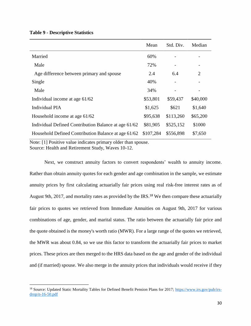
Out of the 962 people in our sample, 60 percent are married primary earners, 72 percent of
whom are male. Of the singles in our analysis, 34 percent are male. In Table 9 we present basic
summary statistics for our sample. Average earnings for those aged 61-62 is $53,800, slightly
higher than the average income in the population aged 55-64, which is $52,350.16 Since we drop
married secondary earners, it is not surprising that the average (and median) income in our sample
is higher. The average PIA of our sample is about $1,600, above the national average PIA
calculated based on the average monthly benefit for those receiving benefits at age 62.17 Finally,
the majority of individuals in the data do not have a significant balance in their defined contribution
plan; however, some have large balances, resulting in a median ($7,650) that is well below the
mean ($107,284). In Appendix A we provide histograms of income and defined contribution
balances at individual and household levels.
15 To estimate the PIA, we apply the bend points in the PIA formula based on the respondent’s Social Security
eligibility year (the year he or she turned 62). 16 Source: United States Census Bureau, Historical Income Tables: People, Table P-10. Age--People (Both Sexes
Combined--All Races) by Median and Mean Income: 1974 to 2015 17 The average monthly benefit for those claiming benefits at age 62 was $1,045 as of December 2015, corresponding
to a PIA of $1,393. Source: Annual Statistical Supplement, 2016, Table 5.A1.1: “Number and average monthly benefit
for retired workers, by age and sex, December 2015”
https://www.ssa.gov/policy/docs/statcomps/supplement/2016/5a.html#table5.a1.1
30
Table 9 - Descriptive Statistics
Mean Std. Div. Median
Married 60% - -
Male 72% - -
Age difference between primary and spouse 2.4 6.4 2
Single 40% - -
Male 34% - -
Individual income at age 61/62 $53,801 $59,437 $40,000
Individual PIA $1,625 $621 $1,640
Household income at age 61/62 $95,638 $113,260 $65,200
Individual Defined Contribution Balance at age 61/62 $81,905 $525,152 $1000
Household Defined Contribution Balance at age 61/62 $107,284 $556,898 $7,650
Note: [1] Positive value indicates primary older than spouse.
Source: Health and Retirement Study, Waves 10-12.
Next, we construct annuity factors to convert respondents’ wealth to annuity income.
Rather than obtain annuity quotes for each gender and age combination in the sample, we estimate
annuity prices by first calculating actuarially fair prices using real risk-free interest rates as of
August 9th, 2017, and mortality rates as provided by the IRS.18 We then compare these actuarially
fair prices to quotes we retrieved from Immediate Annuities on August 9th, 2017 for various
combinations of age, gender, and marital status. The ratio between the actuarially fair price and
the quote obtained is the money's worth ratio (MWR). For a large range of the quotes we retrieved,
the MWR was about 0.84, so we use this factor to transform the actuarially fair prices to market
prices. These prices are then merged to the HRS data based on the age and gender of the individual
and (if married) spouse. We also merge in the annuity prices that individuals would receive if they
18 Source: Updated Static Mortality Tables for Defined Benefit Pension Plans for 2017; https://www.irs.gov/pub/irs-
drop/n-16-50.pdf

31
were to start the annuity one year, three years, and eight years later (corresponding to retiring at
age 63, 65 and 70).
To calculate the returns to working longer we must make several assumptions. First, we
assume that regardless of the retirement choice of the primary earner, the spouse will retire at age
62 and receive 75% of their Social Security benefits. Holding the secondary earner’s retirement
and claiming age constant ensures that the increase in retirement income is entirely driven by the
primary’s retirement choice. The specific age at which the spouse claims Social Security and
retires would not change the results substantially; we just need it to be constant across the scenarios
compared. Second, we assume future wage growth is zero, so that the wage in future years of work
is the same as the wage at age 61/62. Third, we allow for the additional year to count towards one
of the wages included in the AIME calculation; that is, if the last wage earned is among the top 35
years of indexed earnings it will increase the individual’s AIME. Fourth, we assume real asset
returns are 0%, and that the defined contribution saving rate during additional years of work is
equal to 9% of annual salary. Fifth, as in the stylized examples, we assume claiming Social
Security and retirement are simultaneous. Sixth, we assume people annuitize their defined
contribution balance when they retire.19 Finally, we ignore potential income from defined benefit
pensions.
With the assumptions we have made, we can compute the returns to working longer for
each individual. Since the returns will differ across people based on individual factors, we plot in
Figures 3 through 8 the distributions of the returns to working longer and consider how these vary
based on individual characteristics and assumptions made.
19 The initial defined contribution balance is the sum of the current balance in plans 1 through 4 (variable names
R`w’DCBAL1- R`w’DCBAL4, where `w’ indicates the wave number. We used the latest available balance we have
in the data. For many individuals since is the balance prior to age 61/62.

32
In Figure 3 we plot the distribution of returns to working longer for our full sample. Returns
vary from about 3% to double-digit returns. The mean and median are 7.4% and 6.9%,
respectively, not much higher than the 6.7% returns found in Table 3 for a 62 year old stylized
worker.
Figure 3: Returns to Working One Year Longer
Note: Returns are calculated for all primary earners in the HRS data aged
61/62 in waves 10, 11 or 12. Calculations assume returns on wealth are
equal to zero and a 9 percent contribution rate.
Figure 4 below presents the distribution of the returns to working longer based on income
quartiles, corresponding to the analysis of stylized workers at different income levels in Section
2.4. The only difference is that our stylized workers were assumed to be 66, while the empirical
analysis is done for individuals aged 62. The figure shows that returns tend to be more disperse
for higher income households relative to lower income households. While the mean return for all
income groups is about the same, the majority of households at the lowest income quartile

33
receive returns around 6-8% returns, while middle and top income quartile households’ returns
are more spread out.
Figure 4: Returns to Working One Year Longer by Income Quartiles
Note: Returns are calculated for all primary earners in the HRS data aged
61/62 in waves 10, 11 or 12. Calculations assume returns on wealth are
equal to zero and a 9 percent contribution rate. We exclude in the graph
returns below 3% and above 14% to focus attention on the majority of the
return distribution.
Figure 5 illustrates the impact of working for an additional three or eight years (as
opposed to one year). Unsurprisingly, working eight years longer has a much larger impact on
retirement living standards than working one year longer. The figure suggests that working eight
additional years will increase retirement income by at least 40% and above 100% for some
individuals. There is a large mass of people gaining just below 80%, which corresponds well
with our stylized example in Table 3.

34
Figure 5: Returns to Working Longer by Duration of Extension
Note: Returns are calculated for all primary earners in the HRS data aged
61/62 in waves 10, 11 or 12. Calculations assume returns on wealth are
equal to zero and a 9 percent contribution rate.
Who gains the most from working eight additional years? To answer that question, Table
10 presents the means of a number of variables for the full sample as well as those in the top 5
percent of the returns distribution. Those with higher returns are less likely to be married. They
also have shorter working histories (less than 35 on average), so part of the return from working
longer likely comes from the impact of the additional year’s salary on AIME. But the biggest
difference between the full sample and those at the top of the returns distribution is the average
defined contribution balance at age 62. The average DC balance of the top 5 percent is a fifth of
the average DC balance of the full sample. When low-balance individuals save 9% of their

35
annual wage during additional years of work (where their final annual wage is about the same in
the two groups), they more than triple their savings. With the change in annuity prices due to age
they more than quadruple their annuity income.
Table 10 – Characteristics of Full Sample versus Highest-Return Individuals
Full
sample
Top 95 percentile
No. of Observations 962 171
% Married 60% 39%
% Male 57% 40%
Annuity Price at 62 $29.1 $28.2
Annuity Price at 70 $22.5 $21.8
Years Worked 39 33
Last Household Income $95,638 $91,531
AIME at 62 $3,745 $2,615
AIME at 70 $4,186 $3,556
DC Balance at 62 $107,284 $19,015
DC Balance at 70 $140,424 $65,020
% Change from Delay 31% 242%
Annuity Monthly Value at 62 $303 $54
Annuity Monthly Value at 70 $517 $245
% Change from Delay 70% 355%
Monthly Household SS Income at 62 $1,521 $958
Monthly Household SS Income at 70 $2,585 $2,066
% Change from Delay 70% 110%
Average % Income Change from
Delay
81% 128%

36
Next, we consider the impact of changing the real asset return assumption. In Table 2 we
saw that when real asset returns increase, the gains to working longer increase as well, although
the impact was small. Figure 6 reflects the same conclusion for our sample. The figure presents
the distribution of returns to working an additional year for individuals at age 62 assuming zero
and five percent asset returns. The distributions are fairly similar at all asset returns with a slight
shift to the right as the asset returns rate increases.
Figure 6: Returns to Working One Year Longer by Real Asset Return Environment
Note: Returns are calculated for all primary earners in the HRS data aged
61/62 in waves 10, 11 or 12. Calculations assume a 9 percent contribution
rate. We exclude in the graph returns below 3% and above 14% to focus
attention on the majority of the return distribution.
In Figure 7 we consider the impact of marital status and gender on the returns to working
longer. Our stylized examples presented in Figure 2 indicated that returns are highest for single
males and lowest for couples. The main driver of this result is the change in annuity price from
delaying an additional year. As expected, the distribution of returns for couples lies slightly to
the left of the distributions for singles. However, in contrast to the stylized examples, single

37
females seem to have larger returns. This might occur because single women in the data have
lower incomes on average than single men, while our stylized examples assumed the same
income for both genders.
Figure 7: Returns to Working One Year Longer by Marital Status and Gender
Note: Returns are calculated for all primary earners in the HRS data aged
61/62 in waves 10, 11 or 12. Calculations assume returns on wealth are
equal to zero and a 9 percent contribution rate.

38
Figure 8: Marginal Incentive to Work an Additional Year
Note: Returns are calculated for all primary earners in the HRS data aged
61/62 in waves 10, 11 or 12. Calculations assume returns on wealth are
equal to zero and a 9 percent contribution rate. Graph includes observations
from the 5th to the 90th percentiles so that each bin includes at least 10
people, in accordance with the restricted HRS data use requirements.
Figure 8 shows the marginal incentive to work, as described in Section 3.6, for our HRS
sample. The median primary earner would receive the equivalent of an extra 29.9% of final year
salary if they were to work an additional year. The 25th and 75th percentiles of this distribution
are 18.3% and 44.4% of final salary, respectively. These results suggest that the Social Security
formula provides a sizeable incentive to delay the onset of Social Security and work longer if the
claiming and retirement decisions are tied together. Understanding this incentive provides
valuable information for workers considering options to boost retirement living standards.

39
5. Conclusion.
Our primary conclusion is that working longer is relatively powerful compared to saving
more for most people. Our initial base case stylized primary earner illustrates why that is the
case. Recall, the base case was someone who started saving for retirement at age 36, who
contributed a total of 9 percent of earnings to a 401(k) plan, who experienced 0 percent real wage
growth and 0 percent real investment returns during their career, and who retired and
commenced Social Security at age 66. Sustainable income in retirement was composed
primarily of Social Security (81 percent), with a smaller proportion coming from the annuitized
401(k) balance (19 percent). By working longer and deferring the commencement of Social
Security, the primary earner could increase both the Social Security monthly benefit and the
annuitized monthly income. That is, working longer affects both components of retirement
income. On the other hand, by saving more, the primary earner could only increase the
annuitized 401(k) balance, which makes up only 19 percent of retirement income. For instance,
by saving 10 percent rather than 9 percent for the entire 30 years, the affordable 401(k) annuity
increases by 11.11%, but that increase applies to only 19 percent of retirement income.
Therefore, it is not surprising that only 3 months of additional work generates the same increase
in retirement income as 30 years of saving an additional one percentage point of earnings. When
we look at different rates of return on assets, different ages of retirement and at singles vs.
married primary earners, the general result remains that working 3 to 6 extra months has an
equivalent impact on the affordable sustainable standard of living as saving one percentage point
more for 30 years. Increases in saving that start later in life have a proportionately smaller
impact, increasing the power of working longer for individuals who are reoptimizing close to
retirement.

40
Our empirical results are understandably nosier than our stylized results, but at the same
time very consistent with them. They reflect that for most people, Social Security supplies a
large fraction of retirement income. Deferring retirement increases all sources of retirement
income, whereas saving more only increases the relatively small contribution of annuitized
defined contribution balances. The saving adjustment required to achieve a particular increase in
retirement income is larger the later in the career that the adjustment takes place. In other words,
saving more gets less powerful as the career progresses, but deferring retirement remains equally
powerful.
Obviously, the choice of whether to work longer, save more, or adjust the retirement
standard of living depends on individuals’ preferences. However, by laying out the tradeoffs, we
hope that this paper helps people plan for their retirement and helps them reoptimize their
retirement plans in the face of changing circumstances. Not everyone has control over their
retirement date, but certainly many people do. We have shown that career length is a powerful
determinant of the standard of living in retirement. Roughly speaking, deferring retirement by
one year allows for an 8 percent higher standard of living for a couple and the subsequent
survivor. The effect compounds for two, three, and four-year work extensions. The impact of
working longer relative to saving more increases as individuals get closer to retirement. Thus,
working longer may be a much more attractive option than saving more for people who are
reoptimizing their retirement plans ten or so years before retirement.

41
References:
Attanasio, O. P., & Weber, G. (2010). “Consumption and Saving: Models of Intertemporal
Allocation and Their Implications for Public Policy,” Journal of Economic Literature,
48(3), 693–751.
Blau, D. M. (2008). “Retirement and Consumption in a Life Cycle Model,” Journal of Labor
Economics, 26(1), 35–71.
Carroll, C. D. (1997). “Buffer-Stock Saving and the Life Cycle/Permanent Income Hypothesis,”
The Quarterly Journal of Economics, 112(1), 1–55.
Carroll, C. D. (2009). “Precautionary saving and the marginal propensity to consume out of
permanent income.” Journal of Monetary Economics, 56(6), 780–790.
Carroll, C. D., Hall, R. E., & Zeldes, S. P. (1992). “The Buffer-Stock Theory of Saving: Some
Macroeconomic Evidence,” Brookings Papers on Economic Activity, 1992(2), 61–156.
Deaton, A. (1991). “Saving and Liquidity Constraints,” Econometrica, 59(5), 1221–1248.
Friedman, M. (1957). “A Theory of the Consumption Function,” NBER. Retrieved from
http://papers.nber.org/books/frie57-1
Gustman, A. L., & Steinmeier, T. (2008). How Changes in Social Security Affect Recent
Retirement Trends (Working Paper No. 14105). National Bureau of Economic Research.
Retrieved from http://www.nber.org/papers/w14105
Gustman, A. L., & Steinmeier, T. L. (1986). “A Structural Retirement Model,” Econometrica,
54(3), 555–584. https://doi.org/10.2307/1911308
Gustman, A. L., & Steinmeier, T. L. (2015). “Effects of social security policies on benefit
claiming, retirement and saving,” Journal of Public Economics, 129, 51–62.
Haan, P., & Prowse, V. (2014). “Longevity, life-cycle behavior and pension reform,” Journal of
Econometrics, 178, Part 3, 582–601. https://doi.org/10.1016/j.jeconom.2013.08.038
Heffetz, O., & Reeves, D. B. (2016). Difficulty to Reach Respondents and Nonresponse Bias:
Evidence from Large Government Surveys (Working Paper No. 22333). National Bureau
of Economic Research. Retrieved from http://www.nber.org/papers/w22333
Kotlikoff, L. J. (2008). “Economics’ Approach to Financial Planning,” Journal of Financial
Planning; Denver, 21(3), 42-44-52.
Modigliani, F. (1966). “The Life Cycle Hypothesis of Saving, The Demand for Wealth and the
Supply of Capital,” Social Research, 33(2), 160–217.

42
Olson, J. (1999). “Linkages With Data From Social Security Administrative Records in the
Health and Retirement Study,” Social Security Bulletin, 62(2), 73–85.
Scholz, J. K., & Seshadri, A. (2009). What Replacement Rates Should Households Use? (No.
WP 2009-214). Michigan Retirement Research Center. Retrieved from
https://deepblue.lib.umich.edu/bitstream/handle/2027.42/65069/wp214.pdf?sequence=1&
isAllowed=y
Shefrin, H. M., & Thaler, R. H. (1988). “The Behavioral Life-Cycle Hypothesis,” Economic
Inquiry; Huntington Beach, 26(4), 609.

43
Appendix
A.1 Individual and Household Income
The following figures illustrates the distribution of individual and household income for the
people in our sample.
Figure A1: Individual and Household Income Distribution when Individual is of Age 61/62
Primary Income at age 61/62 Household Income when Primary is at age
61/62
Source: Health and Retirement Study, Waves 10-12.

44
A.2 Defined Contribution Balances
The following figures illustrate the distribution of household defined contribution balances both
including and excluding zero balances. The graph on the left indicates that, zero balances are
very common, comprising almost 60% of the balances in our sample. The graph on the right
illustrates that even when zero balances are removed, the distribution of balances is skewed to
the left, with most balances below $50,000. This indicates that for most households, Social
Security is likely the main source of income during retirement. (Note that our analysis ignores
any defined benefit income.)
Figure A2: Household Defined Contribution Balance Distribution when Primary is of Age
61/62
Household DC Balance When Primary is
61/62
Household DC Balance When Primary is
61/62, Zeros Removed
Source: Health and Retirement Study, Waves 10-12.

45
A.3 Career Length
Figure A.3 illustrates the distribution of career lengths in our sample. The majority of individuals
have a career length of 35 years or more, suggesting that additional years of work will have at
most a small impact on AIME.
Figure A3: Distribution of Career Lengths, as of Age 61/62