Embed Size (px)
Citation preview
The Portable Extensible Toolkit for Scientific computingThis talk: http://59A2.org/files/20110817-ACTS.pdf
Jed Brown
Mathematics and Computer Science Division, Argonne National Laboratory
ACTS 2011-08-17
Jed Brown (ANL) PETSc ACTS 2011-08-17 1 / 130

Outline
1 Introduction
2 Installation
3 Programming modelCollective semanticsOptions Database
4 Core PETSc Components and Algorithms PrimerLinear Algebra background/theoryNonlinear solvers: SNESStructured grid distribution: DAPreconditioningMatrix ReduxDebugging
Jed Brown (ANL) PETSc ACTS 2011-08-17 2 / 130

Requests
• Tell me if you do not understand
• Tell me if an example does not work
• Suggest better wording, figures, organization• Follow up:
• Configuration issues, private: [email protected]• Public questions: [email protected]• Me: [email protected]
Jed Brown (ANL) PETSc ACTS 2011-08-17 3 / 130

Introduction
Outline
1 Introduction
2 Installation
3 Programming modelCollective semanticsOptions Database
4 Core PETSc Components and Algorithms PrimerLinear Algebra background/theoryNonlinear solvers: SNESStructured grid distribution: DAPreconditioningMatrix ReduxDebugging
Jed Brown (ANL) PETSc ACTS 2011-08-17 4 / 130

Introduction
1991 1995 2000 2005 2010
PETSc-1MPI-1 MPI-2
PETSc-2 PETSc-3Barry
BillLois
SatishDinesh
HongKrisMatt
VictorDmitry
LisandroJedShri
Jed Brown (ANL) PETSc ACTS 2011-08-17 5 / 130

Introduction
Portable Extensible Toolkit for Scientific computing
• Architecture• tightly coupled (e.g. XT5, BG/P, Earth Simulator)• loosely coupled such as network of workstations• GPU clusters (many vector and sparse matrix kernels)
• Operating systems (Linux, Mac, Windows, BSD, proprietary Unix)
• Any compiler
• Real/complex, single/double/quad precision, 32/64-bit int
• Usable from C, C++, Fortran 77/90, Python, and MATLAB
• Free to everyone (BSD-style license), open development
• 500B unknowns, 75% weak scalability on Jaguar (225k cores)and Jugene (295k cores)
• Same code runs performantly on a laptop
• No iPhone support
Jed Brown (ANL) PETSc ACTS 2011-08-17 6 / 130

Introduction
Portable Extensible Toolkit for Scientific computing
Philosophy: Everything has a plugin architecture
• Vectors, Matrices, Coloring/ordering/partitioning algorithms
• Preconditioners, Krylov accelerators
• Nonlinear solvers, Time integrators
• Spatial discretizations/topology∗
ExampleVendor supplies matrix format and associated preconditioner, distributescompiled shared library. Application user loads plugin at runtime, no sourcecode in sight.
Jed Brown (ANL) PETSc ACTS 2011-08-17 7 / 130

Introduction
Portable Extensible Toolkit for Scientific computing
Algorithms, (parallel) debugging aids, low-overhead profiling
ComposabilityTry new algorithms by choosing from product space and composing existingalgorithms (multilevel, domain decomposition, splitting).
Experimentation
• It is not possible to pick the solver a priori.What will deliver best/competitive performance for a given physics,discretization, architecture, and problem size?
• PETSc’s response: expose an algebra of composition so new solvers canbe created at runtime.
• Important to keep solvers decoupled from physics and discretizationbecause we also experiment with those.
Jed Brown (ANL) PETSc ACTS 2011-08-17 8 / 130
Introduction
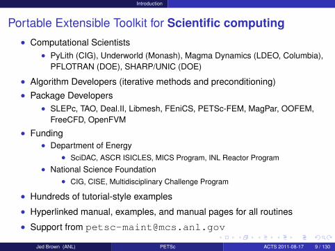
Portable Extensible Toolkit for Scientific computing• Computational Scientists
• PyLith (CIG), Underworld (Monash), Magma Dynamics (LDEO, Columbia),PFLOTRAN (DOE), SHARP/UNIC (DOE)
• Algorithm Developers (iterative methods and preconditioning)• Package Developers
• SLEPc, TAO, Deal.II, Libmesh, FEniCS, PETSc-FEM, MagPar, OOFEM,FreeCFD, OpenFVM
• Funding• Department of Energy
• SciDAC, ASCR ISICLES, MICS Program, INL Reactor Program• National Science Foundation
• CIG, CISE, Multidisciplinary Challenge Program
• Hundreds of tutorial-style examples
• Hyperlinked manual, examples, and manual pages for all routines
• Support from [email protected]
Jed Brown (ANL) PETSc ACTS 2011-08-17 9 / 130

Introduction
The Role of PETSc
Developing parallel, nontrivial PDE solvers that de-liver high performance is still difficult and requiresmonths (or even years) of concentrated effort.
PETSc is a toolkit that can ease these difficulties andreduce the development time, but it is not a black-boxPDE solver, nor a silver bullet.
— Barry Smith
Jed Brown (ANL) PETSc ACTS 2011-08-17 10 / 130

Installation
Outline
1 Introduction
2 Installation
3 Programming modelCollective semanticsOptions Database
4 Core PETSc Components and Algorithms PrimerLinear Algebra background/theoryNonlinear solvers: SNESStructured grid distribution: DAPreconditioningMatrix ReduxDebugging
Jed Brown (ANL) PETSc ACTS 2011-08-17 11 / 130

Installation
Downloading
• http://mcs.anl.gov/petsc, download tarball• We will use Mecurial in this tutorial:
• http://mercurial.selenic.com• Debian/Ubuntu: $ aptitude install mercurial• Fedora: $ yum install mercurial
• Get the PETSc release• $ hg clone \
http://petsc.cs.iit.edu/petsc/releases/petsc-3.1
• $ cd petsc-3.1• $ hg clone
http://petsc.cs.iit.edu/petsc/releases/BuildSystem-3.1 \config/BuildSystem
• Get the latest bug fixes with $ hg pull --update
Jed Brown (ANL) PETSc ACTS 2011-08-17 12 / 130

Installation
Configuration
Basic configuration
• $ export PETSC_DIR=$PWD PETSC_ARCH=mpich-gcc-dbg
• $ ./configure --with-shared \--with-blas-lapack-dir=/usr \--download-mpich,ml,hypre
• $ make all test
• Other common options•• --with-mpi-dir=/path/to/mpi• --with-scalar-type=<real or complex>• --with-precision=<single,double,longdouble>• --with-64-bit-indices• --download-umfpack,mumps,scalapack,blacs,parmetis
• reconfigure at any time with$ mpich-gcc-dbg/conf/reconfigure-mpich-gcc-dbg.py \
--new-options
Jed Brown (ANL) PETSc ACTS 2011-08-17 13 / 130

Installation
Automatic Downloads• Most packages can be automatically
• Downloaded• Configured and Built (in $PETSC_DIR/externalpackages)• Installed with PETSc
• Currently works for• petsc4py• PETSc documentation utilities (Sowing, lgrind, c2html)• BLAS, LAPACK, BLACS, ScaLAPACK, PLAPACK• MPICH, MPE, Open MPI• ParMetis, Chaco, Jostle, Party, Scotch, Zoltan• MUMPS, Spooles, SuperLU, SuperLU_Dist, UMFPack, pARMS• PaStiX, BLOPEX, FFTW, SPRNG• Prometheus, HYPRE, ML, SPAI• Sundials• Triangle, TetGen, FIAT, FFC, Generator• HDF5, Boost
Can also use --with-xxx=/path/to/your/installJed Brown (ANL) PETSc ACTS 2011-08-17 14 / 130

Installation
An optimized build
• $ mpich-gcc-dbg/conf/reconfigure-mpich-gcc-dbg.pyPETSC_ARCH=mpich-gcc-opt
--with-debugging=0 && make PETSC_ARCH=mpich-gcc-opt
• What does --with-debugging=1 (default) do?• Keeps debugging symbols (of course)• Maintains a stack so that errors produce a full stack trace (even SEGV)• Does lots of integrity checking of user input• Places sentinels around allocated memory to detect memory errors• Allocates related memory chunks separately (to help find memory bugs)• Keeps track of and reports unused options• Keeps track of and reports allocated memory that is not freed
-malloc_dump
Jed Brown (ANL) PETSc ACTS 2011-08-17 15 / 130

Installation
Compiling an example
• $ hg clonehttp://petsc.cs.iit.edu/petsc/tutorials/CSCS10
• $ cd CSCS10
• $ hg update 1
• $ make
• $ ./pbratu -help | less
Jed Brown (ANL) PETSc ACTS 2011-08-17 16 / 130
Programming model
Outline
1 Introduction
2 Installation
3 Programming modelCollective semanticsOptions Database
4 Core PETSc Components and Algorithms PrimerLinear Algebra background/theoryNonlinear solvers: SNESStructured grid distribution: DAPreconditioningMatrix ReduxDebugging
Jed Brown (ANL) PETSc ACTS 2011-08-17 17 / 130

Programming model
PETSc Structure
Jed Brown (ANL) PETSc ACTS 2011-08-17 18 / 130

Programming model
Flow Control for a PETSc Application
Timestepping Solvers (TS)
Preconditioners (PC)
Nonlinear Solvers (SNES)
Linear Solvers (KSP)
Function
EvaluationPostprocessing
Jacobian
Evaluation
Application
Initialization
Main Routine
PETSc
Jed Brown (ANL) PETSc ACTS 2011-08-17 19 / 130
Programming model Collective semantics
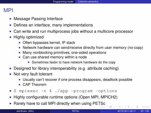
MPI• Message Passing Interface• Defines an interface, many implementations• Can write and run multiprocess jobs without a multicore processor• Highly optimized
• Often bypasses kernel, IP stack• Network hardware can send/receive directly from user memory (no-copy)• Many nonblocking primitives, one-sided operations• Can use shared memory within a node
• Sometimes faster to have network hardware do the copy
• Designed for library interoperability (e.g. attribute caching)• Not very fault tolerant
• Usually can’t recover if one process disappears, deadlock possible• CAP Theorem
• $ mpiexec -n 4 ./app -program -options
• Highly configurable runtime options (Open MPI, MPICH2)• Rarely have to call MPI directly when using PETSc
Jed Brown (ANL) PETSc ACTS 2011-08-17 20 / 130

Programming model Collective semantics
MPI communicators• Opaque object, defines process group and synchronization channel• PETSc objects need an MPI_Comm in their constructor
• PETSC_COMM_SELF for serial objects• PETSC_COMM_WORLD common, but not required
• Can split communicators, spawn processes on new communicators, etc• Operations are one of
• Not Collective: VecGetLocalSize(), MatSetValues()• Logically Collective: KSPSetType(), PCMGSetCycleType()
• checked when running in debug mode• Neighbor-wise Collective: VecScatterBegin(), MatMult()
• Point-to-point communication between two processes• Neighbor collectives in upcoming MPI-3
• Collective: VecNorm(), MatAssemblyBegin(), KSPCreate()
• Global communication, synchronous• Non-blocking collectives in upcoming MPI-3
• Deadlock if some process doesn’t participate (e.g. wrong order)
Jed Brown (ANL) PETSc ACTS 2011-08-17 21 / 130
Programming model Collective semantics
Advice from Bill Gropp
You want to think about how you decompose your datastructures, how you think about them globally. [...] If you werebuilding a house, you’d start with a set of blueprints that giveyou a picture of what the whole house looks like. You wouldn’tstart with a bunch of tiles and say. “Well I’ll put this tile downon the ground, and then I’ll find a tile to go next to it.” But alltoo many people try to build their parallel programs by creatingthe smallest possible tiles and then trying to have the structureof their code emerge from the chaos of all these little pieces.You have to have an organizing principle if you’re going tosurvive making your code parallel.
(http://www.rce-cast.com/Podcast/rce-28-mpich2.html)
Jed Brown (ANL) PETSc ACTS 2011-08-17 22 / 130

Programming model Options Database
ObjectsMat A;PetscInt m,n,M,N;MatCreate(comm,&A);MatSetSizes(A,m,n,M,N); /* or PETSC_DECIDE */MatSetOptionsPrefix(A,"foo_");MatSetFromOptions(A);/* Use A */MatView(A,PETSC_VIEWER_DRAW_WORLD);MatDestroy(A);
• Mat is an opaque object (pointer to incomplete type)• Assignment, comparison, etc, are cheap
• What’s up with this “Options” stuff?• Allows the type to be determined at runtime: -foo_mat_type sbaij• Inversion of Control similar to “service locator”,
related to “dependency injection”• Other options (performance and semantics) can be changed at runtime
under -foo_mat_Jed Brown (ANL) PETSc ACTS 2011-08-17 23 / 130

Programming model Options Database
Basic PetscObject Usage
Every object in PETSc supports a basic interfaceFunction Operation
Create() create the objectGet/SetName() name the objectGet/SetType() set the implementation type
Get/SetOptionsPrefix() set the prefix for all optionsSetFromOptions() customize object from the command line
SetUp() preform other initializationView() view the object
Destroy() cleanup object allocationAlso, all objects support the -help option.
Jed Brown (ANL) PETSc ACTS 2011-08-17 24 / 130

Programming model Options Database
Ways to set options
• Command line
• Filename in the third argument of PetscInitialize()
• ∼/.petscrc• $PWD/.petscrc• $PWD/petscrc• PetscOptionsInsertFile()• PetscOptionsInsertString()• PETSC_OPTIONS environment variable
• command line option -options_file [file]
Jed Brown (ANL) PETSc ACTS 2011-08-17 25 / 130
Programming model Options Database
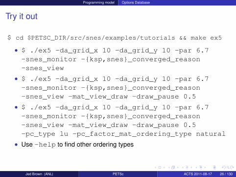
Try it out
$ cd $PETSC_DIR/src/snes/examples/tutorials && make ex5
• $ ./ex5 -da_grid_x 10 -da_grid_y 10 -par 6.7-snes_monitor -ksp,snes_converged_reason-snes_view
• $ ./ex5 -da_grid_x 10 -da_grid_y 10 -par 6.7-snes_monitor -ksp,snes_converged_reason-snes_view -mat_view_draw -draw_pause 0.5
• $ ./ex5 -da_grid_x 10 -da_grid_y 10 -par 6.7-snes_monitor -ksp,snes_converged_reason-snes_view -mat_view_draw -draw_pause 0.5-pc_type lu -pc_factor_mat_ordering_type natural
• Use -help to find other ordering types
Jed Brown (ANL) PETSc ACTS 2011-08-17 26 / 130

Programming model Options Database
In parallel
• $ mpiexec -n 4./ex5 -da_grid_x 10 -da_grid_y 10 -par 6.7-snes_monitor -ksp,snes_converged_reason-snes_view -sub_pc_type lu
• How does the performance change as you• vary the number of processes (up to 32 or 64)?• increase the problem size?• use an inexact subdomain solve?• try an overlapping method: -pc_type asm -pc_asm_overlap 2• simulate a big machine: -pc_asm_blocks 512• change the Krylov method: -ksp_type ibcgs• use algebraic multigrid: -pc_type hypre• use smoothed aggregation multigrid: -pc_type ml
Jed Brown (ANL) PETSc ACTS 2011-08-17 27 / 130

Core/Algorithms
Outline
1 Introduction
2 Installation
3 Programming modelCollective semanticsOptions Database
4 Core PETSc Components and Algorithms PrimerLinear Algebra background/theoryNonlinear solvers: SNESStructured grid distribution: DAPreconditioningMatrix ReduxDebugging
Jed Brown (ANL) PETSc ACTS 2011-08-17 28 / 130
Core/Algorithms
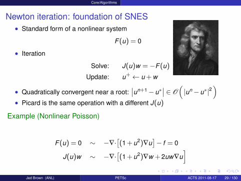
Newton iteration: foundation of SNES• Standard form of a nonlinear system
F(u) = 0
• Iteration
Solve: J(u)w =−F(u)
Update: u+← u + w
• Quadratically convergent near a root:∣∣un+1−u∗
∣∣ ∈ O(|un−u∗|2
)• Picard is the same operation with a different J(u)
Example (Nonlinear Poisson)
F(u) = 0 ∼ −∇·[(1 + u2)∇u
]− f = 0
J(u)w ∼ −∇·[(1 + u2)∇w + 2uw∇u
]Jed Brown (ANL) PETSc ACTS 2011-08-17 29 / 130

Core/Algorithms Linear Algebra background/theory
Matrices
Definition (Matrix)A matrix is a linear transformation between finite dimensional vector spaces.
Definition (Forming a matrix)Forming or assembling a matrix means defining it’s action in terms of entries(usually stored in a sparse format).
Jed Brown (ANL) PETSc ACTS 2011-08-17 30 / 130

Core/Algorithms Linear Algebra background/theory
Important matrices
1 Sparse (e.g. discretization of a PDE operator)
2 Inverse of anything interesting B = A−1
3 Jacobian of a nonlinear function Jy = limε→0F(x+εy)−F(x)
ε
4 Fourier transform F ,F−1
5 Other fast transforms, e.g. Fast Multipole Method
6 Low rank correction B = A + uvT
7 Schur complement S = D−CA−1B
8 Tensor product A = ∑e Aex ⊗Ae
y ⊗Aez
9 Linearization of a few steps of an explicit integrator
Jed Brown (ANL) PETSc ACTS 2011-08-17 31 / 130

Core/Algorithms Linear Algebra background/theory
Important matrices
1 Sparse (e.g. discretization of a PDE operator)
2 Inverse of anything interesting B = A−1
3 Jacobian of a nonlinear function Jy = limε→0F(x+εy)−F(x)
ε
4 Fourier transform F ,F−1
5 Other fast transforms, e.g. Fast Multipole Method
6 Low rank correction B = A + uvT
7 Schur complement S = D−CA−1B
8 Tensor product A = ∑e Aex ⊗Ae
y ⊗Aez
9 Linearization of a few steps of an explicit integrator
• These matrices are dense. Never form them.
Jed Brown (ANL) PETSc ACTS 2011-08-17 31 / 130

Core/Algorithms Linear Algebra background/theory
Important matrices
1 Sparse (e.g. discretization of a PDE operator)
2 Inverse of anything interesting B = A−1
3 Jacobian of a nonlinear function Jy = limε→0F(x+εy)−F(x)
ε
4 Fourier transform F ,F−1
5 Other fast transforms, e.g. Fast Multipole Method
6 Low rank correction B = A + uvT
7 Schur complement S = D−CA−1B
8 Tensor product A = ∑e Aex ⊗Ae
y ⊗Aez
9 Linearization of a few steps of an explicit integrator
• These are not very sparse. Don’t form them.
Jed Brown (ANL) PETSc ACTS 2011-08-17 31 / 130

Core/Algorithms Linear Algebra background/theory
Important matrices
1 Sparse (e.g. discretization of a PDE operator)
2 Inverse of anything interesting B = A−1
3 Jacobian of a nonlinear function Jy = limε→0F(x+εy)−F(x)
ε
4 Fourier transform F ,F−1
5 Other fast transforms, e.g. Fast Multipole Method
6 Low rank correction B = A + uvT
7 Schur complement S = D−CA−1B
8 Tensor product A = ∑e Aex ⊗Ae
y ⊗Aez
9 Linearization of a few steps of an explicit integrator
• None of these matrices “have entries”
Jed Brown (ANL) PETSc ACTS 2011-08-17 31 / 130
Core/Algorithms Linear Algebra background/theory
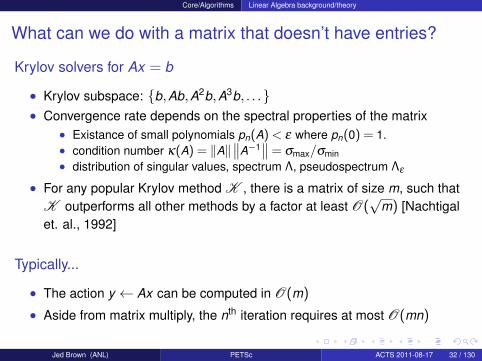
What can we do with a matrix that doesn’t have entries?
Krylov solvers for Ax = b
• Krylov subspace: b,Ab,A2b,A3b, . . .• Convergence rate depends on the spectral properties of the matrix
• Existance of small polynomials pn(A) < ε where pn(0) = 1.• condition number κ(A) = ‖A‖
∥∥A−1∥∥= σmax/σmin
• distribution of singular values, spectrum Λ, pseudospectrum Λε
• For any popular Krylov method K , there is a matrix of size m, such thatK outperforms all other methods by a factor at least O(
√m) [Nachtigal
et. al., 1992]
Typically...
• The action y ← Ax can be computed in O(m)
• Aside from matrix multiply, the nth iteration requires at most O(mn)
Jed Brown (ANL) PETSc ACTS 2011-08-17 32 / 130

Core/Algorithms Linear Algebra background/theory
GMRES
Brute force minimization of residual in b,Ab,A2b, . . .1 Use Arnoldi to orthogonalize the nth subspace, producing
AQn = Qn+1Hn
2 Minimize residual in this space by solving the overdetermined system
Hnyn = e(n+1)1
using QR-decomposition, updated cheaply at each iteration.
Properties
• Converges in n steps for all right hand sides if there exists a polynomial ofdegree n such that ‖pn(A)‖< tol and pn(0) = 1.
• Residual is monotonically decreasing, robust in practice
• Restarted variants are used to bound memory requirements
Jed Brown (ANL) PETSc ACTS 2011-08-17 33 / 130

Core/Algorithms Linear Algebra background/theory
The p-Bratu equation• 2-dimensional model problem
−∇·(|∇u|p−2
∇u)−λeu− f = 0, 1≤ p≤ ∞, λ < λcrit(p)
Singular or degenerate when ∇u = 0, turning point at λcrit.
• Regularized variant
−∇·(η∇u)−λeu− f = 0
η(γ) = (ε2 + γ)
p−22 γ(u) =
12|∇u|2
• Jacobian
J(u)w ∼−∇·[(η1 + η
′∇u⊗∇u)∇w
]−λeuw
η′ =
p−22
η/(ε2 + γ)
Physical interpretation: conductivity tensor flattened in direction ∇u
Jed Brown (ANL) PETSc ACTS 2011-08-17 34 / 130

Core/Algorithms Nonlinear solvers: SNES
Flow Control for a PETSc Application
Timestepping Solvers (TS)
Preconditioners (PC)
Nonlinear Solvers (SNES)
Linear Solvers (KSP)
Function
EvaluationPostprocessing
Jacobian
Evaluation
Application
Initialization
Main Routine
PETSc
Jed Brown (ANL) PETSc ACTS 2011-08-17 35 / 130
Core/Algorithms Nonlinear solvers: SNES
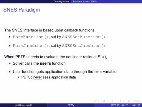
SNES Paradigm
The SNES interface is based upon callback functions
• FormFunction(), set by SNESSetFunction()
• FormJacobian(), set by SNESSetJacobian()
When PETSc needs to evaluate the nonlinear residual F(x),
• Solver calls the user’s function
• User function gets application state through the ctx variable• PETSc never sees application data
Jed Brown (ANL) PETSc ACTS 2011-08-17 36 / 130

Core/Algorithms Nonlinear solvers: SNES
SNES Function
The user provided function which calculates the nonlinear residual hassignature
PetscErrorCode (*func)(SNES snes,Vec x,Vec r,void *ctx)
x: The current solution
r: The residualctx: The user context passed to SNESSetFunction()
• Use this to pass application information, e.g. physical constants
Jed Brown (ANL) PETSc ACTS 2011-08-17 37 / 130

Core/Algorithms Nonlinear solvers: SNES
SNES JacobianThe user provided function which calculates the Jacobian has signature
PetscErrorCode (*func)(SNES snes,Vec x,Mat *J,Mat *M,MatStructure *flag,void *ctx)
x: The current solution
J: The Jacobian
M: The Jacobian preconditioning matrix (possibly J itself)ctx: The user context passed to SNESSetFunction()
• Use this to pass application information, e.g. physical constants
• Possible MatStructure values are:• SAME_NONZERO_PATTERN• DIFFERENT_NONZERO_PATTERN
Alternatively, you can use
• a builtin sparse finite difference approximation (“coloring”)
• automatic differentiation (ADIC/ADIFOR)Jed Brown (ANL) PETSc ACTS 2011-08-17 38 / 130

Core/Algorithms Structured grid distribution: DA
Distributed Array
• Interface for topologically structured grids• Defines (topological part of) a finite-dimensional function space
• Get an element from this space: DACreateGlobalVector()
• Provides parallel layout• Refinement and coarsening
• DARefineHierarchy()
• Ghost value coherence• DAGlobalToLocalBegin()
• Matrix preallocation:• DAGetMatrix()
Jed Brown (ANL) PETSc ACTS 2011-08-17 39 / 130

Core/Algorithms Structured grid distribution: DA
Ghost ValuesTo evaluate a local function f (x), each process requires
• its local portion of the vector x
• its ghost values, bordering portions of x owned by neighboring processes
Local Node
Ghost Node
Jed Brown (ANL) PETSc ACTS 2011-08-17 40 / 130
Core/Algorithms Structured grid distribution: DA
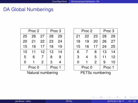
DA Global Numberings
Proc 2 Proc 325 26 27 28 2920 21 22 23 2415 16 17 18 1910 11 12 13 145 6 7 8 90 1 2 3 4
Proc 0 Proc 1Natural numbering
Proc 2 Proc 321 22 23 28 2918 19 20 26 2715 16 17 24 256 7 8 13 143 4 5 11 120 1 2 9 10
Proc 0 Proc 1PETSc numbering
Jed Brown (ANL) PETSc ACTS 2011-08-17 41 / 130

Core/Algorithms Structured grid distribution: DA
DA Global vs. Local Numbering
• Global: Each vertex has a unique id belongs on a unique process• Local: Numbering includes vertices from neighboring processes
• These are called ghost vertices
Proc 2 Proc 3X X X X XX X X X X12 13 14 15 X8 9 10 11 X4 5 6 7 X0 1 2 3 X
Proc 0 Proc 1Local numbering
Proc 2 Proc 321 22 23 28 2918 19 20 26 2715 16 17 24 256 7 8 13 143 4 5 11 120 1 2 9 10
Proc 0 Proc 1Global numbering
Jed Brown (ANL) PETSc ACTS 2011-08-17 42 / 130
Core/Algorithms Structured grid distribution: DA
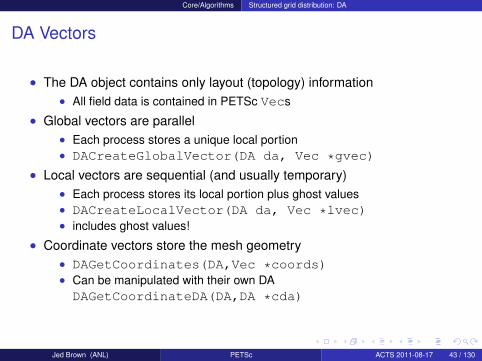
DA Vectors
• The DA object contains only layout (topology) information• All field data is contained in PETSc Vecs
• Global vectors are parallel• Each process stores a unique local portion• DACreateGlobalVector(DA da, Vec *gvec)
• Local vectors are sequential (and usually temporary)• Each process stores its local portion plus ghost values• DACreateLocalVector(DA da, Vec *lvec)• includes ghost values!
• Coordinate vectors store the mesh geometry• DAGetCoordinates(DA,Vec *coords)• Can be manipulated with their own DADAGetCoordinateDA(DA,DA *cda)
Jed Brown (ANL) PETSc ACTS 2011-08-17 43 / 130

Core/Algorithms Structured grid distribution: DA
Updating Ghosts
Two-step process enables overlappingcomputation and communication
• DAGlobalToLocalBegin(da, gvec, mode, lvec)• gvec provides the data• mode is either INSERT_VALUES or ADD_VALUES• lvec holds the local and ghost values
• DAGlobalToLocalEnd(da, gvec, mode, lvec)• Finishes the communication
The process can be reversed with DALocalToGlobal().
Jed Brown (ANL) PETSc ACTS 2011-08-17 44 / 130

Core/Algorithms Structured grid distribution: DA
DA Stencils
Both the box stencil and star stencil are available.
proc 0 proc 1
proc 10
proc 0 proc 1
proc 10
Box Stencil Star Stencil
Jed Brown (ANL) PETSc ACTS 2011-08-17 45 / 130
Core/Algorithms Structured grid distribution: DA
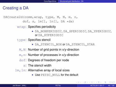
Creating a DA
DACreate2d(comm,wrap, type, M, N, m, n,
dof, s, lm[], ln[], DA *da)
wrap: Specifies periodicity• DA_NONPERIODIC, DA_XPERIODIC, DA_YPERIODIC,
or DA_XYPERIODIC
type: Specifies stencil• DA_STENCIL_BOX or DA_STENCIL_STAR
M,N: Number of grid points in x/y-direction
m,n: Number of processes in x/y-direction
dof: Degrees of freedom per node
s: The stencil widthlm,ln: Alternative array of local sizes
• Use PETSC_NULL for the default
Jed Brown (ANL) PETSc ACTS 2011-08-17 46 / 130
Core/Algorithms Structured grid distribution: DA
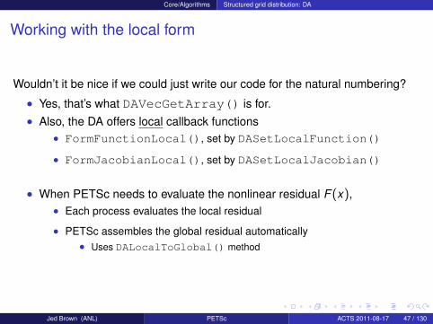
Working with the local form
Wouldn’t it be nice if we could just write our code for the natural numbering?
• Yes, that’s what DAVecGetArray() is for.• Also, the DA offers local callback functions
• FormFunctionLocal(), set by DASetLocalFunction()
• FormJacobianLocal(), set by DASetLocalJacobian()
• When PETSc needs to evaluate the nonlinear residual F(x),• Each process evaluates the local residual
• PETSc assembles the global residual automatically• Uses DALocalToGlobal() method
Jed Brown (ANL) PETSc ACTS 2011-08-17 47 / 130

Core/Algorithms Structured grid distribution: DA
DA Local Function
The user provided function which calculates the nonlinear residual in 2D hassignaturePetscErrorCode (*lfunc)(DALocalInfo *info,
Field **x, Field **r, void *ctx)
info: All layout and numbering informationx: The current solution
• Notice that it is a multidimensional array
r: The residual
ctx: The user context passed to DASetLocalFunction()
The local DA function is activated by calling
SNESSetFunction(snes, r, SNESDAFormFunction, ctx)
Jed Brown (ANL) PETSc ACTS 2011-08-17 48 / 130

Core/Algorithms Structured grid distribution: DA
Bratu Residual Evaluation
−∆u−λeu = 0
BratuResidualLocal(DALocalInfo *info,Field **x,Field **f,UserCtx *user)
/* Not Shown: Handle boundaries *//* Compute over the interior points */for(j = info->ys; j < info->ys+info->ym; j++) for(i = info->xs; i < info->xs+info->xm; i++)
u = x[j][i];u_xx = (2.0*u - x[j][i-1] - x[j][i+1])*hydhx;u_yy = (2.0*u - x[j-1][i] - x[j+1][i])*hxdhy;f[j][i] = u_xx + u_yy - hx*hy*lambda*exp(u);
$PETSC_DIR/src/snes/examples/tutorials/ex5.c
Jed Brown (ANL) PETSc ACTS 2011-08-17 49 / 130

Core/Algorithms Structured grid distribution: DA
Start with 2-Laplacian plus Bratu nonlinearity
• Matrix-free Jacobians, no preconditioning -snes_mf
• $ hg update -r3
• $ ./pbratu -da_grid_x 10 -da_grid_y 10-lambda 6.7 -snes_mf -snes_monitor-ksp_converged_reason
• $ ./pbratu -da_grid_x 20 -da_grid_y 20-lambda 6.7 -snes_mf -snes_monitor-ksp_converged_reason
• $ ./pbratu -da_grid_x 40 -da_grid_y 40-lambda 6.7 -snes_mf -snes_monitor-ksp_converged_reason
• Watch linear and nonlinear convergence
Jed Brown (ANL) PETSc ACTS 2011-08-17 50 / 130
Core/Algorithms Structured grid distribution: DA
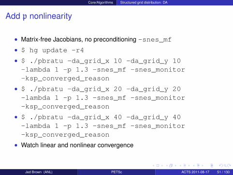
Add p nonlinearity
• Matrix-free Jacobians, no preconditioning -snes_mf
• $ hg update -r4
• $ ./pbratu -da_grid_x 10 -da_grid_y 10-lambda 1 -p 1.3 -snes_mf -snes_monitor-ksp_converged_reason
• $ ./pbratu -da_grid_x 20 -da_grid_y 20-lambda 1 -p 1.3 -snes_mf -snes_monitor-ksp_converged_reason
• $ ./pbratu -da_grid_x 40 -da_grid_y 40-lambda 1 -p 1.3 -snes_mf -snes_monitor-ksp_converged_reason
• Watch linear and nonlinear convergence
Jed Brown (ANL) PETSc ACTS 2011-08-17 51 / 130
Core/Algorithms Preconditioning
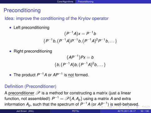
PreconditioningIdea: improve the conditioning of the Krylov operator
• Left preconditioning(P−1A)x = P−1b
P−1b,(P−1A)P−1b,(P−1A)2P−1b, . . .
• Right preconditioning(AP−1)Px = b
b,(P−1A)b,(P−1A)2b, . . .
• The product P−1A or AP−1 is not formed.
Definition (Preconditioner)A preconditioner P is a method for constructing a matrix (just a linearfunction, not assembled!) P−1 = P(A,Ap) using a matrix A and extrainformation Ap, such that the spectrum of P−1A (or AP−1) is well-behaved.
Jed Brown (ANL) PETSc ACTS 2011-08-17 52 / 130
Core/Algorithms Preconditioning
Preconditioning
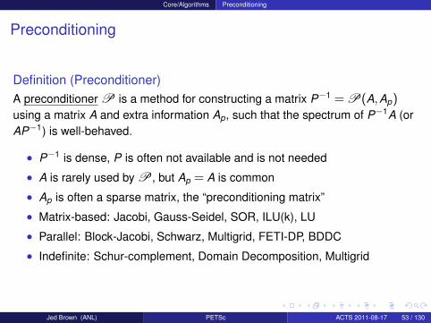
Definition (Preconditioner)A preconditioner P is a method for constructing a matrix P−1 = P(A,Ap)using a matrix A and extra information Ap, such that the spectrum of P−1A (orAP−1) is well-behaved.
• P−1 is dense, P is often not available and is not needed
• A is rarely used by P , but Ap = A is common
• Ap is often a sparse matrix, the “preconditioning matrix”
• Matrix-based: Jacobi, Gauss-Seidel, SOR, ILU(k), LU
• Parallel: Block-Jacobi, Schwarz, Multigrid, FETI-DP, BDDC
• Indefinite: Schur-complement, Domain Decomposition, Multigrid
Jed Brown (ANL) PETSc ACTS 2011-08-17 53 / 130
Core/Algorithms Preconditioning
Questions to ask when you see a matrix
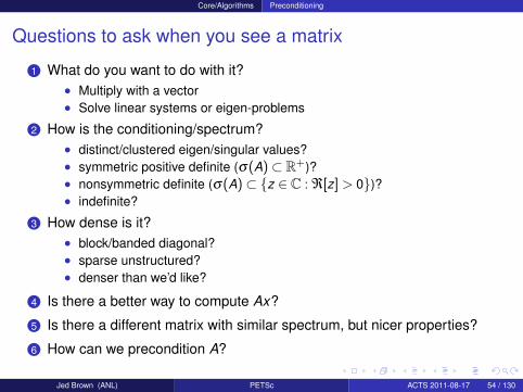
1 What do you want to do with it?• Multiply with a vector• Solve linear systems or eigen-problems
2 How is the conditioning/spectrum?• distinct/clustered eigen/singular values?• symmetric positive definite (σ(A)⊂ R+)?• nonsymmetric definite (σ(A)⊂ z ∈ C : ℜ[z] > 0)?• indefinite?
3 How dense is it?• block/banded diagonal?• sparse unstructured?• denser than we’d like?
4 Is there a better way to compute Ax?
5 Is there a different matrix with similar spectrum, but nicer properties?
6 How can we precondition A?
Jed Brown (ANL) PETSc ACTS 2011-08-17 54 / 130
Core/Algorithms Preconditioning
Questions to ask when you see a matrix
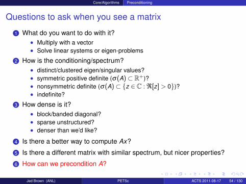
1 What do you want to do with it?• Multiply with a vector• Solve linear systems or eigen-problems
2 How is the conditioning/spectrum?• distinct/clustered eigen/singular values?• symmetric positive definite (σ(A)⊂ R+)?• nonsymmetric definite (σ(A)⊂ z ∈ C : ℜ[z] > 0)?• indefinite?
3 How dense is it?• block/banded diagonal?• sparse unstructured?• denser than we’d like?
4 Is there a better way to compute Ax?
5 Is there a different matrix with similar spectrum, but nicer properties?
6 How can we precondition A?
Jed Brown (ANL) PETSc ACTS 2011-08-17 54 / 130

Core/Algorithms Preconditioning
RelaxationSplit into lower, diagonal, upper parts: A = L + D + U
JacobiCheapest preconditioner: P−1 = D−1
Successive over-relaxation (SOR)
(L +
1ω
D
)xn+1 =
[(1ω−1
)D−U
]xn + ωb
P−1 = k iterations starting with x0 = 0
• Implemented as a sweep
• ω = 1 corresponds to Gauss-Seidel
• Very effective at removing high-frequency components of residual
Jed Brown (ANL) PETSc ACTS 2011-08-17 55 / 130
Core/Algorithms Preconditioning
FactorizationTwo phases
• symbolic factorization: find where fill occurs, only uses sparsity pattern• numeric factorization: compute factors
LU decomposition
• Ultimate preconditioner• Expensive, for m×m sparse matrix with bandwidth b, traditionally requires
O(mb2) time and O(mb) space.
• Bandwidth scales as md−1
d in d-dimensions• Optimal in 2D: O(m · logm) space, O(m3/2) time• Optimal in 3D: O(m4/3) space, O(m2) time
• Symbolic factorization is problematic in parallel
Incomplete LU
• Allow a limited number of levels of fill: ILU(k )• Only allow fill for entries that exceed threshold: ILUT• Very poor scaling in parallel, don’t bother beyond 8 PEs.• No guarantees
Jed Brown (ANL) PETSc ACTS 2011-08-17 56 / 130
Core/Algorithms Preconditioning
1-level Domain decompositionDomain size L, subdomain size H, element size h
Overlapping/Schwarz
• Solve Dirichlet problems on overlapping subdomains
• No overlap: its ∈ O(
L√Hh
)• Overlap δ : its ∈
(L√Hδ
)Neumann-Neumann
• Solve Neumann problems on non-overlapping subdomains
• its ∈ O(
LH (1 + log H
h ))
• Tricky null space issues (floating subdomains)
• Need subdomain matrices, net globally assembled matrix.
• Multilevel variants knock off the leading LH
• Both overlapping and nonoverlapping with this boundJed Brown (ANL) PETSc ACTS 2011-08-17 57 / 130

Core/Algorithms Preconditioning
MultigridHierarchy: Interpolation and restriction operators
I ↑ : Xcoarse→ Xfine I ↓ : Xfine→ Xcoarse
• Geometric: define problem on multiple levels, use grid to compute hierarchy• Algebraic: define problem only on finest level, use matrix structure to build
hierarchy
Galerkin approximationAssemble this matrix: Acoarse = I ↓AfineI ↑
Application of multigrid preconditioner (V -cycle)
• Apply pre-smoother on fine level (any preconditioner)• Restrict residual to coarse level with I ↓
• Solve on coarse level Acoarsex = r• Interpolate result back to fine level with I ↑
• Apply post-smoother on fine level (any preconditioner)
Jed Brown (ANL) PETSc ACTS 2011-08-17 58 / 130

Core/Algorithms Preconditioning
Multigrid convergence properties
• Textbook: P−1A is spectrally equivalent to identity• Constant number of iterations to converge up to discretization error
• Most theory applies to SPD systems• variable coefficients (e.g. discontinuous): low energy interpolants• mesh- and/or physics-induced anisotropy: semi-coarsening/line smoothers• complex geometry: difficult to have meaningful coarse levels
• Deeper algorithmic difficulties• nonsymmetric (e.g. advection, shallow water, Euler)• indefinite (e.g. incompressible flow, Helmholtz)
• Performance considerations• Aggressive coarsening is critical in parallel• Most theory uses SOR smoothers, ILU often more robust• Coarsest level usually solved semi-redundantly with direct solver
• Multilevel Schwarz is essentially the same with different language• assume strong smoothers, emphasize aggressive coarsening
Jed Brown (ANL) PETSc ACTS 2011-08-17 59 / 130

Core/Algorithms Preconditioning
Finite Difference Jacobians
PETSc can compute and explicitly store a Jacobian via 1st-order FD• Dense
• Activated by -snes_fd• Computed by SNESDefaultComputeJacobian()
• Sparse via colorings• Coloring is created by MatFDColoringCreate()• Computed by SNESDefaultComputeJacobianColor()
Can also use Matrix-free Newton-Krylov via 1st-order FD
• Activated by -snes_mf without preconditioning• Activated by -snes_mf_operator with user-defined preconditioning
• Uses preconditioning matrix from SNESSetJacobian()
Jed Brown (ANL) PETSc ACTS 2011-08-17 60 / 130

Core/Algorithms Preconditioning
Add finite difference Jacobian by coloring
• $ hg update -r5
• $ ./pbratu -da_grid_x 10 -da_grid_y 10-lambda 1 -p 1.3 -snes_fd -snes_monitor-ksp_converged_reason
• $ ./pbratu -da_grid_x 10 -da_grid_y 10-lambda 1 -p 1.3 -fd_jacobian -snes_monitor-ksp_converged_reason
• $ ./pbratu -da_grid_x 10 -da_grid_y 10-lambda 1 -p 1.3 -fd_jacobian -snes_monitor-ksp_converged_reason
• Try some different preconditioners (jacobi,sor,asm,hypre,ml)
• Try changing the physical parameters
• May need -mat_fd_type ds
Jed Brown (ANL) PETSc ACTS 2011-08-17 61 / 130
Core/Algorithms Matrix Redux
Matrices, redux
What are PETSc matrices?
• Linear operators on finite dimensional vector spaces. (snarky)
• Fundamental objects for storing stiffness matrices and Jacobians
• Each process locally owns a contiguous set of rows• Supports many data types
• AIJ, Block AIJ, Symmetric AIJ, Block Diagonal, etc.
• Supports structures for many packages• MUMPS, Spooles, SuperLU, UMFPack, Hypre
Jed Brown (ANL) PETSc ACTS 2011-08-17 62 / 130
Core/Algorithms Matrix Redux
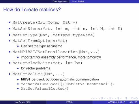
How do I create matrices?
• MatCreate(MPI_Comm, Mat *)
• MatSetSizes(Mat, int m, int n, int M, int N)
• MatSetType(Mat, MatType typeName)
• MatSetFromOptions(Mat)• Can set the type at runtime
• MatMPIBAIJSetPreallocation(Mat,...)• important for assembly performance, more tomorrow
• MatSetBlockSize(Mat, int bs)• for vector problems
• MatSetValues(Mat,...)• MUST be used, but does automatic communication• MatSetValuesLocal(), MatSetValuesStencil()• MatSetValuesBlocked()
Jed Brown (ANL) PETSc ACTS 2011-08-17 63 / 130
Core/Algorithms Matrix Redux
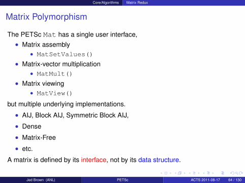
Matrix Polymorphism
The PETSc Mat has a single user interface,• Matrix assembly
• MatSetValues()
• Matrix-vector multiplication• MatMult()
• Matrix viewing• MatView()
but multiple underlying implementations.
• AIJ, Block AIJ, Symmetric Block AIJ,
• Dense
• Matrix-Free
• etc.
A matrix is defined by its interface, not by its data structure.
Jed Brown (ANL) PETSc ACTS 2011-08-17 64 / 130
Core/Algorithms Matrix Redux
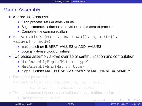
Matrix Assembly• A three step process
• Each process sets or adds values• Begin communication to send values to the correct process• Complete the communication
• MatSetValues(Mat A, m, rows[], n, cols[],values[], mode)
• mode is either INSERT_VALUES or ADD_VALUES• Logically dense block of values
• Two phase assembly allows overlap of communication and computation• MatAssemblyBegin(Mat m, type)• MatAssemblyEnd(Mat m, type)• type is either MAT_FLUSH_ASSEMBLY or MAT_FINAL_ASSEMBLY
• For vector problemsMatSetValuesBlocked(Mat A, m, rows[],
n, cols[], values[], mode)• The same assembly code can build matrices of different format
• choose format at run-time.
Jed Brown (ANL) PETSc ACTS 2011-08-17 65 / 130
Core/Algorithms Matrix Redux
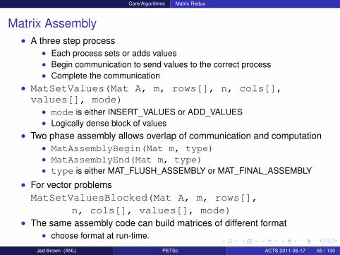
Matrix Assembly• A three step process
• Each process sets or adds values• Begin communication to send values to the correct process• Complete the communication
• MatSetValues(Mat A, m, rows[], n, cols[],values[], mode)
• mode is either INSERT_VALUES or ADD_VALUES• Logically dense block of values
• Two phase assembly allows overlap of communication and computation• MatAssemblyBegin(Mat m, type)• MatAssemblyEnd(Mat m, type)• type is either MAT_FLUSH_ASSEMBLY or MAT_FINAL_ASSEMBLY
• For vector problemsMatSetValuesBlocked(Mat A, m, rows[],
n, cols[], values[], mode)• The same assembly code can build matrices of different format
• choose format at run-time.
Jed Brown (ANL) PETSc ACTS 2011-08-17 65 / 130
Core/Algorithms Matrix Redux
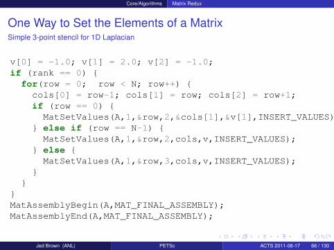
One Way to Set the Elements of a MatrixSimple 3-point stencil for 1D Laplacian
v[0] = -1.0; v[1] = 2.0; v[2] = -1.0;if (rank == 0)
for(row = 0; row < N; row++) cols[0] = row-1; cols[1] = row; cols[2] = row+1;if (row == 0)
MatSetValues(A,1,&row,2,&cols[1],&v[1],INSERT_VALUES); else if (row == N-1)
MatSetValues(A,1,&row,2,cols,v,INSERT_VALUES); else
MatSetValues(A,1,&row,3,cols,v,INSERT_VALUES);
MatAssemblyBegin(A,MAT_FINAL_ASSEMBLY);MatAssemblyEnd(A,MAT_FINAL_ASSEMBLY);
Jed Brown (ANL) PETSc ACTS 2011-08-17 66 / 130

Core/Algorithms Matrix Redux
A Better Way to Set the Elements of a MatrixSimple 3-point stencil for 1D Laplacian
v[0] = -1.0; v[1] = 2.0; v[2] = -1.0;for(row = start; row < end; row++)
cols[0] = row-1; cols[1] = row; cols[2] = row+1;if (row == 0) MatSetValues(A,1,&row,2,&cols[1],&v[1],INSERT_VALUES);
else if (row == N-1) MatSetValues(A,1,&row,2,cols,v,INSERT_VALUES);
else MatSetValues(A,1,&row,3,cols,v,INSERT_VALUES);
MatAssemblyBegin(A, MAT_FINAL_ASSEMBLY);MatAssemblyEnd(A, MAT_FINAL_ASSEMBLY);
Jed Brown (ANL) PETSc ACTS 2011-08-17 67 / 130

Core/Algorithms Matrix Redux
Why Are PETSc Matrices That Way?
• No one data structure is appropriate for all problems• Blocked and diagonal formats provide significant performance benefits• PETSc has many formats and makes it easy to add new data structures
• Assembly is difficult enough without worrying about partitioning• PETSc provides parallel assembly routines• Achieving high performance still requires making most operations local• However, programs can be incrementally developed.• MatPartitioning and MatOrdering can help
• Matrix decomposition in contiguous chunks is simple• Makes interoperation with other codes easier• For other ordering, PETSc provides “Application Orderings” (AO)
Jed Brown (ANL) PETSc ACTS 2011-08-17 68 / 130
Core/Algorithms Matrix Redux
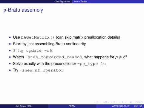
p-Bratu assembly
• Use DAGetMatrix() (can skip matrix preallocation details)
• Start by just assembling Bratu nonlinearity
• $ hg update -r6
• Watch -snes_converged_reason, what happens for p 6= 2?
• Solve exactly with the preconditioner -pc_type lu
• Try -snes_mf_operator
Jed Brown (ANL) PETSc ACTS 2011-08-17 69 / 130

Core/Algorithms Matrix Redux
p-Bratu assembly
• We need to assemble the p part
J(u)w ∼ −∇·[(η1 + η
′∇u⊗∇u)∇w
]• Second part is scary, but what about just using −∇·(η∇w)?
• $ hg update -r7
• Solve exactly with the preconditioner -pc_type lu
• Try -snes_mf_operator
• Refine the grid, change p
• Try algebraic multigrid if available: -pc_type [ml,hypre]
Jed Brown (ANL) PETSc ACTS 2011-08-17 70 / 130

Core/Algorithms Matrix Redux
Does the preconditioner need Newton linearization?
• The anisotropic part looks messy.Is it worth writing the code to assemble that part?
• Easy profiling: -log_summary
• Observation: the Picard linearization uses a “star” (5-point) stencil whileNewton linearization needs a “box” (9-point) stencil.
• Add support for reduced preallocation with a command-line option
• $ hg update -r8
• Compare performance (time, memory, iteration count) of• 5-point Picard-linearization assembled by hand• 5-point Newton-linearized Jacobian computed by coloring• 9-point Newton-linearized Jacobian computed by coloring
Jed Brown (ANL) PETSc ACTS 2011-08-17 71 / 130

Core/Algorithms Debugging
Maybe it’s not worth it, but let’s assemble it anyway
• $ hg update -r9
• Crash!
• You were using the the debug PETSC_ARCH, right?• Launch the debugger
• -start_in_debugger [gdb,dbx,noxterm]• -on_error_attach_debugger [gdb,dbx,noxterm]
• Attach the debugger only to some parallel processes• -debugger_nodes 0,1
• Set the display (often necessary on a cluster)• -display :0
Jed Brown (ANL) PETSc ACTS 2011-08-17 72 / 130
Core/Algorithms Debugging
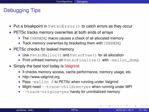
Debugging Tips
• Put a breakpoint in PetscError() to catch errors as they occur• PETSc tracks memory overwrites at both ends of arrays
• The CHKMEMQ macro causes a check of all allocated memory• Track memory overwrites by bracketing them with CHKMEMQ
• PETSc checks for leaked memory• Use PetscMalloc() and PetscFree() for all allocation• Print unfreed memory on PetscFinalize() with -malloc_dump
• Simply the best tool today is Valgrind• It checks memory access, cache performance, memory usage, etc.• http://www.valgrind.org• Pass -malloc 0 to PETSc when running under Valgrind• Might need --trace-children=yes when running under MPI• --track-origins=yes handy for uninitialized memory
Jed Brown (ANL) PETSc ACTS 2011-08-17 73 / 130

Core/Algorithms Debugging
Memory error is gone now
• $ hg update -r10
• Run with -snes_mf_operator -pc_type lu
• Do you see quadratic convergence?
• Hmm, there must be a bug in that mess, where is it?
Jed Brown (ANL) PETSc ACTS 2011-08-17 74 / 130

Core/Algorithms Debugging
Memory error is gone now
• $ hg update -r10
• Run with -snes_mf_operator -pc_type lu
• Do you see quadratic convergence?
• Hmm, there must be a bug in that mess, where is it?
Jed Brown (ANL) PETSc ACTS 2011-08-17 74 / 130

Core/Algorithms Debugging
SNES Test
• PETSc can compute a finite difference Jacobian and compare it to yours• -snes_type test
• Is the difference significant?
• -snes_type test -snes_test_display• Are the entries in the star stencil correct?
• Find which line has the typo
• $ hg update -r11
• Check with -snes_type test
• and -snes_mf_operator -pc_type lu
Jed Brown (ANL) PETSc ACTS 2011-08-17 75 / 130

Application Integration
Outline
5 Application Integration
6 Performance and ScalabilityMemory hierarchyProfiling
Jed Brown (ANL) PETSc ACTS 2011-08-17 76 / 130

Application Integration
Application Integration
• Be willing to experiment with algorithms• No optimality without interplay between physics and algorithmics
• Adopt flexible, extensible programming• Algorithms and data structures not hardwired
• Be willing to play with the real code• Toy models are rarely helpful
• If possible, profile before integration• Automatic in PETSc
Jed Brown (ANL) PETSc ACTS 2011-08-17 77 / 130

Application Integration
Incorporating PETSc into existing codes
• PETSc does not seize main(), does not control output
• Propogates errors from underlying packages, flexible error handling
• Nothing special about MPI_COMM_WORLD• Can wrap existing data structures/algorithms
• MatShell, PCShell, full implementations• VecCreateMPIWithArray()• MatCreateSeqAIJWithArrays()• Use an existing semi-implicit solver as a preconditioner• Usually worthwhile to use native PETSc data structures
unless you have a good reason not to
• Uniform interfaces across languages• C, C++, Fortran 77/90, Python, MATLAB
• Do not have to use high level interfaces (e.g. SNES, TS, DM)• but PETSc can offer more if you do, like MFFD and SNES Test
Jed Brown (ANL) PETSc ACTS 2011-08-17 78 / 130

Application Integration
Integration Stages
• Version Control• It is impossible to overemphasize
• Initialization• Linking to PETSc
• Profiling• Profile before changing• Also incorporate command line processing
• Linear Algebra• First PETSc data structures
• Solvers• Very easy after linear algebra is integrated
Jed Brown (ANL) PETSc ACTS 2011-08-17 79 / 130
Application Integration
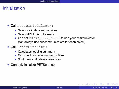
Initialization
• Call PetscInitialize()• Setup static data and services• Setup MPI if it is not already• Can set PETSC_COMM_WORLD to use your communicator
(can always use subcommunicators for each object)
• Call PetscFinalize()• Calculates logging summary• Can check for leaks/unused options• Shutdown and release resources
• Can only initialize PETSc once
Jed Brown (ANL) PETSc ACTS 2011-08-17 80 / 130
Application Integration
Matrix Memory Preallocation• PETSc sparse matrices are dynamic data structures
• can add additional nonzeros freely
• Dynamically adding many nonzeros• requires additional memory allocations• requires copies• can kill performance
• Memory preallocation provides• the freedom of dynamic data structures• good performance
• Easiest solution is to replicate the assembly code• Remove computation, but preserve the indexing code• Store set of columns for each row
• Call preallocation routines for all datatypes• MatSeqAIJSetPreallocation()• MatMPIBAIJSetPreallocation()• Only the relevant data will be used
Jed Brown (ANL) PETSc ACTS 2011-08-17 81 / 130
Application Integration
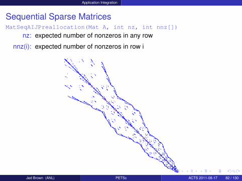
Sequential Sparse MatricesMatSeqAIJPreallocation(Mat A, int nz, int nnz[])
nz: expected number of nonzeros in any row
nnz(i): expected number of nonzeros in row i
Jed Brown (ANL) PETSc ACTS 2011-08-17 82 / 130

Application Integration
Parallel Sparse Matrix• Each process locally owns a submatrix of contiguous global rows• Each submatrix consists of diagonal and off-diagonal parts
proc 5
proc 4
proc 3
proc 2
proc 1
proc 0
diagonal blocks
offdiagonal blocks
• MatGetOwnershipRange(Mat A,int *start,int *end)start: first locally owned row of global matrixend-1: last locally owned row of global matrix
Jed Brown (ANL) PETSc ACTS 2011-08-17 83 / 130

Application Integration
Parallel Sparse Matrices
MatMPIAIJPreallocation(Mat A, int dnz, int dnnz[],int onz, int onnz[])
dnz: expected number of nonzeros in any row in the diagonal block
dnnz(i): expected number of nonzeros in row i in the diagonal block
onz: expected number of nonzeros in any row in the offdiagonal portion
onnz(i): expected number of nonzeros in row i in the offdiagonal portion
Jed Brown (ANL) PETSc ACTS 2011-08-17 84 / 130

Application Integration
Verifying Preallocation
• Use runtime option -info
• Output:[proc #] Matrix size: %d X %d; storage space:%d unneeded, %d used[proc #] Number of mallocs during MatSetValues( )is %d
Jed Brown (ANL) PETSc ACTS 2011-08-17 85 / 130

Application Integration
Block and symmetric formats
• BAIJ• Like AIJ, but uses static block size• Preallocation is like AIJ, but just one index per block
• SBAIJ• Only stores upper triangular part• Preallocation needs number of nonzeros in upper triangular
parts of on- and off-diagonal blocks
• MatSetValuesBlocked()• Better performance with blocked formats• Also works with scalar formats, if MatSetBlockSize() was called• Variants MatSetValuesBlockedLocal(),MatSetValuesBlockedStencil()
• Change matrix format at runtime, don’t need to touch assembly code
Jed Brown (ANL) PETSc ACTS 2011-08-17 86 / 130
Application Integration
Linear SolversKrylov Methods
• Using PETSc linear algebra, just add:• KSPSetOperators(KSP ksp, Mat A, Mat M,MatStructure flag)
• KSPSolve(KSP ksp, Vec b, Vec x)
• Can access subobjects• KSPGetPC(KSP ksp, PC *pc)
• Preconditioners must obey PETSc interface• Basically just the KSP interface
• Can change solver dynamically from the command line, -ksp_type
Jed Brown (ANL) PETSc ACTS 2011-08-17 87 / 130
Application Integration
Nonlinear SolversNewton and Picard Methods
• Using PETSc linear algebra, just add:• SNESSetFunction(SNES snes, Vec r, residualFunc,void *ctx)
• SNESSetJacobian(SNES snes, Mat A, Mat M, jacFunc,void *ctx)
• SNESSolve(SNES snes, Vec b, Vec x)
• Can access subobjects• SNESGetKSP(SNES snes, KSP *ksp)
• Can customize subobjects from the cmd line• Set the subdomain preconditioner to ILU with -sub_pc_type ilu
Jed Brown (ANL) PETSc ACTS 2011-08-17 88 / 130
Performance and Scalability
Outline
5 Application Integration
6 Performance and ScalabilityMemory hierarchyProfiling
Jed Brown (ANL) PETSc ACTS 2011-08-17 89 / 130

Performance and Scalability
Bottlenecks of (Jacobian-free) Newton-Krylov
• Matrix assembly• integration/fluxes: FPU• insertion: memory/branching
• Preconditioner setup• coarse level operators• overlapping subdomains• (incomplete) factorization
• Preconditioner application• triangular solves/relaxation: memory• coarse levels: network latency
• Matrix multiplication• Sparse storage: memory• Matrix-free: FPU
• Globalization
Jed Brown (ANL) PETSc ACTS 2011-08-17 90 / 130

Performance and Scalability
Scalability definitions
Strong scalability• Fixed problem size
• execution time T inverselyproportional to number ofprocessors p
Weak scalability• Fixed problem size per processor
• execution time constant asproblem size increases
Jed Brown (ANL) PETSc ACTS 2011-08-17 91 / 130

Performance and Scalability
Scalability Warning
The easiest way to make software scalableis to make it sequentially inefficient.
(Gropp 1999)
• We really want efficient software• Need a performance model
• memory bandwidth and latency• algorithmically critical operations (e.g. dot products, scatters)• floating point unit
• Scalability shows marginal benefit of adding more cores, nothing more
• Constants hidden in the choice of algorithm
• Constants hidden in implementation
Jed Brown (ANL) PETSc ACTS 2011-08-17 92 / 130
Performance and Scalability Memory hierarchy
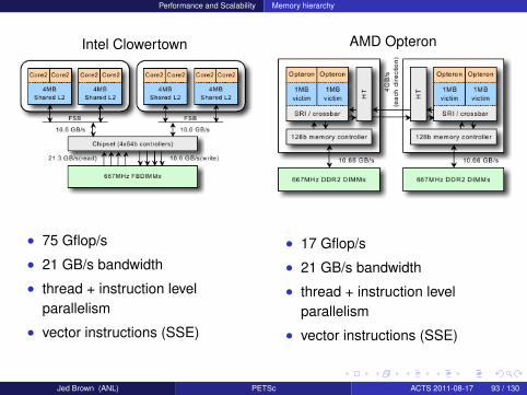
Intel Clowertown
• 75 Gflop/s
• 21 GB/s bandwidth
• thread + instruction levelparallelism
• vector instructions (SSE)
AMD Opteron
• 17 Gflop/s
• 21 GB/s bandwidth
• thread + instruction levelparallelism
• vector instructions (SSE)
Jed Brown (ANL) PETSc ACTS 2011-08-17 93 / 130

Performance and Scalability Memory hierarchy
Hardware capabilities
Floating point unitRecent Intel: each core can issue
• 1 packed add (latency 3)
• 1 packed mult (latency 5)
• One can include an aligned read
• Out of Order execution
• Peak: 10 Gflop/s (double)
Memory
• ∼ 250 cycle latency
• 5.3 GB/s bandwidth
• 1 double load / 3.7 cycles
• Pay by the cache line (32/64 B)
• L2 cache: ∼ 10 cycle latency
(Oliker et al. 2008)Jed Brown (ANL) PETSc ACTS 2011-08-17 94 / 130

Performance and Scalability Memory hierarchy
(Oliker et al. Multi-core Optimization of Sparse Matrix Vector Multiplication, 2008)
Jed Brown (ANL) PETSc ACTS 2011-08-17 95 / 130

Performance and Scalability Memory hierarchy
Sparse Mat-Vec performance model
Compressed Sparse Row format (AIJ)For m×n matrix with N nonzeros
ai row starts, length m + 1
aj column indices, length N, range [0,n−1)
aa nonzero entries, length N, scalar values
y ← y + Axfor ( i =0; i <m; i ++)
for ( j = a i [ i ] ; j < a i [ i + 1 ] ; j ++)y [ i ] += aa [ j ] ∗ x [ a j [ j ] ] ;
• One add and one multiply per inner loop
• Scalar aa[j] and integer aj[j] only used once
• Must load aj[j] to read from x, may not reuse cache well
Jed Brown (ANL) PETSc ACTS 2011-08-17 96 / 130

Performance and Scalability Memory hierarchy
Memory Bandwidth• Stream Triad benchmark (GB/s): w ← αx + y
• Sparse matrix-vector product: 6 bytes per flop
Jed Brown (ANL) PETSc ACTS 2011-08-17 97 / 130

Performance and Scalability Memory hierarchy
Optimizing Sparse Mat-Vec
• Order unknows so that vector reuses cache (Reverse Cuthill-McKee)• Optimal: (2 flops)(bandwidth)
sizeof(Scalar)+sizeof(Int)• Usually improves strength of ILU and SOR
• Coalesce indices for adjacent rows with same nonzero pattern (Inodes)• Optimal: (2 flops)(bandwidth)
sizeof(Scalar)+sizeof(Int)/i• Can do block SOR (much stronger than scalar SOR)• Default in PETSc, turn off with -mat_no_inode• Requires ordering unknowns so that fields are interlaced, this is (much)
better for memory use anyway
• Use explicit blocking, hold one index per block (BAIJ format)• Optimal: (2 flops)(bandwidth)
sizeof(Scalar)+sizeof(Int)/b2
• Block SOR and factorization• Symbolic factorization works with blocks (much cheaper)• Very regular memory access, unrolled dense kernels• Faster insertion: MatSetValuesBlocked()
Jed Brown (ANL) PETSc ACTS 2011-08-17 98 / 130

Performance and Scalability Memory hierarchy
Performance of assembled versus unassembled
1 2 3 4 5 6 7polynomial order
102
103
104
byte
s/re
sult
1 2 3 4 5 6 7polynomial order
102
103
104
flops
/resu
lt
tensor b = 1tensor b = 3tensor b = 5assembled b = 1assembled b = 3assembled b = 5
• Arithmetic intensity for Qp elements• ≤ 1
4 (assembled), ≈ 10 (unassembled), ≈ 4 (hardware)
• store Jacobian information at Quass quadrature points, can use AD
Jed Brown (ANL) PETSc ACTS 2011-08-17 99 / 130
Performance and Scalability Memory hierarchy
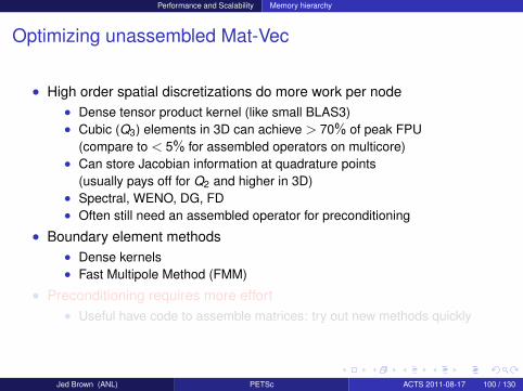
Optimizing unassembled Mat-Vec
• High order spatial discretizations do more work per node• Dense tensor product kernel (like small BLAS3)• Cubic (Q3) elements in 3D can achieve > 70% of peak FPU
(compare to < 5% for assembled operators on multicore)• Can store Jacobian information at quadrature points
(usually pays off for Q2 and higher in 3D)• Spectral, WENO, DG, FD• Often still need an assembled operator for preconditioning
• Boundary element methods• Dense kernels• Fast Multipole Method (FMM)
• Preconditioning requires more effort• Useful have code to assemble matrices: try out new methods quickly
Jed Brown (ANL) PETSc ACTS 2011-08-17 100 / 130
Performance and Scalability Memory hierarchy
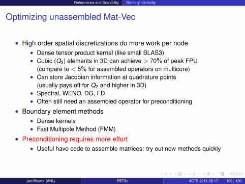
Optimizing unassembled Mat-Vec
• High order spatial discretizations do more work per node• Dense tensor product kernel (like small BLAS3)• Cubic (Q3) elements in 3D can achieve > 70% of peak FPU
(compare to < 5% for assembled operators on multicore)• Can store Jacobian information at quadrature points
(usually pays off for Q2 and higher in 3D)• Spectral, WENO, DG, FD• Often still need an assembled operator for preconditioning
• Boundary element methods• Dense kernels• Fast Multipole Method (FMM)
• Preconditioning requires more effort• Useful have code to assemble matrices: try out new methods quickly
Jed Brown (ANL) PETSc ACTS 2011-08-17 100 / 130
Performance and Scalability Profiling
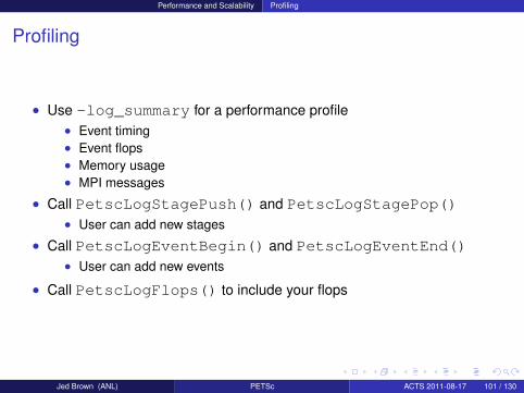
Profiling
• Use -log_summary for a performance profile• Event timing• Event flops• Memory usage• MPI messages
• Call PetscLogStagePush() and PetscLogStagePop()• User can add new stages
• Call PetscLogEventBegin() and PetscLogEventEnd()• User can add new events
• Call PetscLogFlops() to include your flops
Jed Brown (ANL) PETSc ACTS 2011-08-17 101 / 130
Performance and Scalability Profiling
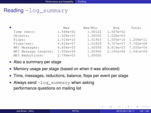
Reading -log_summary
• Max Max/Min Avg TotalTime (sec): 1.548e+02 1.00122 1.547e+02Objects: 1.028e+03 1.00000 1.028e+03Flops: 1.519e+10 1.01953 1.505e+10 1.204e+11Flops/sec: 9.814e+07 1.01829 9.727e+07 7.782e+08MPI Messages: 8.854e+03 1.00556 8.819e+03 7.055e+04MPI Message Lengths: 1.936e+08 1.00950 2.185e+04 1.541e+09MPI Reductions: 2.799e+03 1.00000
• Also a summary per stage
• Memory usage per stage (based on when it was allocated)
• Time, messages, reductions, balance, flops per event per stage
• Always send -log_summary when askingperformance questions on mailing list
Jed Brown (ANL) PETSc ACTS 2011-08-17 102 / 130

Performance and Scalability Profiling
Communication Costs
• Reductions: usually part of Krylov method, latency limited• VecDot• VecMDot• VecNorm• MatAssemblyBegin• Change algorithm (e.g. IBCGS)
• Point-to-point (nearest neighbor), latency or bandwidth• VecScatter• MatMult• PCApply• MatAssembly• SNESFunctionEval• SNESJacobianEval• Compute subdomain boundary fluxes redundantly• Ghost exchange for all fields at once• Better partition
Jed Brown (ANL) PETSc ACTS 2011-08-17 103 / 130
Representative examples and algorithms
Outline
7 Representative examples and algorithmsHydrostatic IceDriven cavity
8 Hard problems
9 What’s new for PETSc-3.2?Improved multiphysics supportTime integrationVariational inequalities
Jed Brown (ANL) PETSc ACTS 2011-08-17 104 / 130

Representative examples and algorithms Hydrostatic Ice
Hydrostatic equations for ice sheet flow• Valid when wx uz , independent of basal friction (Schoof&Hindmarsh
2010)• Eliminate p and w from Stokes by incompressibility:
3D elliptic system for u = (u,v)
−∇ ·[
η
(4ux + 2vy uy + vx uz
uy + vx 2ux + 4vy vz
)]+ ρg∇h = 0
η(θ ,γ) =B(θ)
2(γ0 + γ)
1−n2n , n≈ 3
γ = u2x + v2
y + uxvy +14
(uy + vx )2 +14
u2z +
14
v2z
and slip boundary σ ·n = β 2u where
β2(γb) = β
20 (ε
2b + γb)
m−12 , 0 <m≤ 1
γb =12
(u2 + v2)
• Q1 FEM with Newton-Krylov-Multigrid solver in PETSc:src/snes/examples/tutorials/ex48.cJed Brown (ANL) PETSc ACTS 2011-08-17 105 / 130

Representative examples and algorithms Hydrostatic Ice
Jed Brown (ANL) PETSc ACTS 2011-08-17 106 / 130

Representative examples and algorithms Hydrostatic Ice
Some Multigrid Options
• -dmmg_grid_sequencce: [FALSE]Solve nonlinear problems on coarse grids to get initial guess
• -pc_mg_galerkin: [FALSE]Use Galerkin process to compute coarser operators
• -pc_mg_type: [FULL](choose one of) MULTIPLICATIVE ADDITIVE FULL KASKADE
• -mg_coarse_ksp,pc_*control the coarse-level solver
• -mg_levels_ksp,pc_*control the smoothers on levels
• -mg_levels_3_ksp,pc_*control the smoother on specific level
• These also work with ML’s algebraic multigrid.
Jed Brown (ANL) PETSc ACTS 2011-08-17 107 / 130

Representative examples and algorithms Hydrostatic Ice
What is this doing?
• mpiexec -n 4 ./ex48 -M 16 -P 2 -da_refine_hierarchy_x 1,8,8-da_refine_hierarchy_y 2,1,1 -da_refine_hierarchy_z 2,1,1-dmmg_grid_sequence 1 -dmmg_view -log_summary-ksp_converged_reason -ksp_gmres_modifiedgramschmidt-ksp_monitor -ksp_rtol 1e-2-pc_mg_type multiplicative-mg_coarse_pc_type lu -mg_levels_0_pc_type lu-mg_coarse_pc_factor_mat_solver_package mumps-mg_levels_0_pc_factor_mat_solver_package mumps-mg_levels_1_sub_pc_type cholesky-snes_converged_reason -snes_monitor -snes_stol 1e-12-thi_L 80e3 -thi_alpha 0.05 -thi_friction_m 0.3-thi_hom x -thi_nlevels 4
• What happens if you remove -dmmg_grid_sequence?
• What about solving with block Jacobi, ASM, or algebraic multigrid?
Jed Brown (ANL) PETSc ACTS 2011-08-17 108 / 130

Representative examples and algorithms Driven cavity
SNES ExampleDriven Cavity
• Velocity-vorticity formulation
• Flow driven by lid and/or bouyancy• Logically regular grid
• Parallelized with DA
• Finite difference discretization
• Authored by David Keyes
Jed Brown (ANL) PETSc ACTS 2011-08-17 109 / 130

Representative examples and algorithms Driven cavity
SNES ExampleDriven Cavity Application Context
/∗ Col located at each node ∗ /typedef struct
PetscScalar u , v , omega , temp ; F i e l d ;
typedef struct /∗ phys i ca l parameters ∗ /
PassiveReal l i d v e l o c i t y , p rand t l , grashof ;/∗ co lo r p l o t s o f the s o l u t i o n ∗ /
PetscTruth draw_contours ; AppCtx ;
Jed Brown (ANL) PETSc ACTS 2011-08-17 110 / 130
Representative examples and algorithms Driven cavity
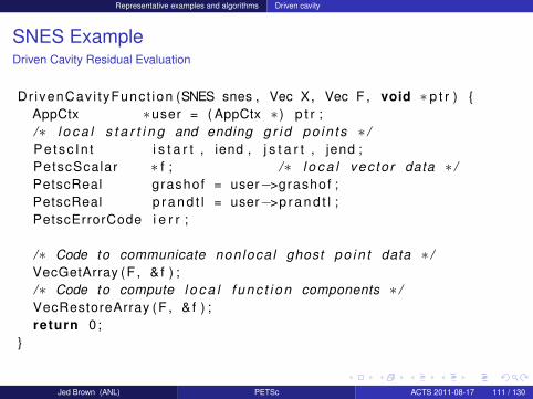
SNES ExampleDriven Cavity Residual Evaluation
Dr ivenCav i tyFunct ion (SNES snes , Vec X, Vec F , void ∗ p t r ) AppCtx ∗user = ( AppCtx ∗ ) p t r ;/∗ l o c a l s t a r t i n g and ending g r i d po in t s ∗ /Petsc In t i s t a r t , iend , j s t a r t , jend ;PetscScalar ∗ f ; /∗ l o c a l vec to r data ∗ /PetscReal grashof = user−>grashof ;PetscReal p r a n d t l = user−>p r a n d t l ;PetscErrorCode i e r r ;
/∗ Code to communicate non loca l ghost po i n t data ∗ /VecGetArray (F , & f ) ;/∗ Code to compute l o c a l f u n c t i o n components ∗ /VecRestoreArray (F , & f ) ;return 0;
Jed Brown (ANL) PETSc ACTS 2011-08-17 111 / 130
Representative examples and algorithms Driven cavity
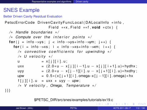
SNES ExampleBetter Driven Cavity Residual Evaluation
PetscErrorCode DrivenCavi tyFuncLocal ( DALocalInfo ∗ i n fo ,F i e l d ∗∗x , F i e l d ∗∗ f , void ∗ c tx )
/∗ Handle boundaries ∗ //∗ Compute over the i n t e r i o r po in t s ∗ /for ( j = in fo−>ys ; j < in fo−>ys+ in fo−>ym; j ++)
for ( i = in fo−>xs ; i < in fo−>xs+ in fo−>xm; i ++) /∗ convect ive c o e f f i c i e n t s f o r upwinding ∗ //∗ U v e l o c i t y ∗ /u = x [ j ] [ i ] . u ;uxx = (2 .0∗u − x [ j ] [ i −1].u − x [ j ] [ i + 1 ] . u )∗hydhx ;uyy = (2 .0∗u − x [ j −1][ i ] . u − x [ j + 1 ] [ i ] . u )∗hxdhy ;upw = 0.5∗ ( x [ j + 1 ] [ i ] . omega−x [ j −1][ i ] . omega)∗hxf [ j ] [ i ] . u = uxx + uyy − upw ;/∗ V v e l o c i t y , Omega, Temperature ∗ /
$PETSC_DIR/src/snes/examples/tutorials/ex19.c
Jed Brown (ANL) PETSc ACTS 2011-08-17 112 / 130

Representative examples and algorithms Driven cavity
Running the driven cavity
• ./ex19 -lidvelocity 100 -grashof 1e2 -da_grid_x16 -da_grid_y 16 -snes_monitor -dmmg_view-nlevels 3
• ./ex19 -lidvelocity 100 -grashof 1e4 -da_grid_x16 -da_grid_y 16 -snes_monitor -dmmg_view-nlevels 3
• ./ex19 -lidvelocity 100 -grashof 1e5 -da_grid_x16 -da_grid_y 16 -snes_monitor -dmmg_view-nlevels 3
• Uh oh, we have convergence problems
• Run with -snes_monitor_convergence
• Does -dmmg_grid_sequence help?
Jed Brown (ANL) PETSc ACTS 2011-08-17 113 / 130

Representative examples and algorithms Driven cavity
Why isn’t SNES converging?
• The Jacobian is wrong (maybe only in parallel)• Check with -snes_type test and -snes_mf_operator-pc_type lu
• The linear system is not solved accurately enough• Check with -pc_type lu• Check -ksp_monitor_true_residual, try right preconditioning
• The Jacobian is singular with inconsistent right side• Use MatNullSpace to inform the KSP of a known null space• Use a different Krylov method or preconditioner
• The nonlinearity is just really strong• Run with -info or -snes_ls_monitor (petsc-dev) to see line search• Try using trust region instead of line search -snes_type tr• Try grid sequencing if possible• Use a continuation
Jed Brown (ANL) PETSc ACTS 2011-08-17 114 / 130

Representative examples and algorithms Driven cavity
Globalizing the lid-driven cavity
Pseudotransient continuation continuation (Ψtc)
• Do linearly implicit backward-Euler steps, driven by steady-state residual
• Clever way to adjust step sizes to retain quadratic convergence interminal phase
• Implemented in src/snes/examples/tutorials/ex27.c
• $ make runex27
• Make the method linearly implicit: -snes_max_it 1• Compare required number of linear iterations
• Try increasing -lidvelocity, -grashof, and problem size
• Coffey, Kelley, and Keyes, Pseudotransient continuation and differentialalgebraic equations, SIAM J. Sci. Comp, 2003.
Jed Brown (ANL) PETSc ACTS 2011-08-17 115 / 130
Hard problems
Outline
7 Representative examples and algorithmsHydrostatic IceDriven cavity
8 Hard problems
9 What’s new for PETSc-3.2?Improved multiphysics supportTime integrationVariational inequalities
Jed Brown (ANL) PETSc ACTS 2011-08-17 116 / 130

Hard problems
Splitting for Multiphysics[A BC D
][xy
]=
[fg
]• Relaxation: -pc_fieldsplit_type[additive,multiplicative,symmetric_multiplicative][
AD
]−1 [AC D
]−1 [A
1
]−1(
1−[
A B1
][AC D
]−1)
• Gauss-Seidel inspired, works when fields are loosely coupled• Factorization: -pc_fieldsplit_type schur[
A BS
]−1[1
CA−1 1
]−1
, S = D−CA−1B
• robust (exact factorization), can often drop lower block• how to precondition S which is usually dense?
• interpret as differential operators, use approximate commutators
Jed Brown (ANL) PETSc ACTS 2011-08-17 117 / 130
Hard problems
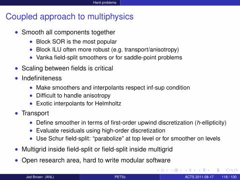
Coupled approach to multiphysics
• Smooth all components together• Block SOR is the most popular• Block ILU often more robust (e.g. transport/anisotropy)• Vanka field-split smoothers or for saddle-point problems
• Scaling between fields is critical• Indefiniteness
• Make smoothers and interpolants respect inf-sup condition• Difficult to handle anisotropy• Exotic interpolants for Helmholtz
• Transport• Define smoother in terms of first-order upwind discretization (h-ellipticity)• Evaluate residuals using high-order discretization• Use Schur field-split: “parabolize” at top level or for smoother on levels
• Multigrid inside field-split or field-split inside multigrid
• Open research area, hard to write modular software
Jed Brown (ANL) PETSc ACTS 2011-08-17 118 / 130

Hard problems
“Physics-based” preconditioners (semi-implicit method)Shallow water with stiff gravity waveh is hydrostatic pressure, u is velocity,
√gh is fast wave speed
ht − (uh)x = 0
(uh)t + (u2h +12
gh2)x = 0Semi-implicit methodSuppress spatial discretization, discretize in time, implicitly for the terms contributing tothe gravity wave
hn+1−hn
∆t+ (uh)n+1
x = 0
(uh)n+1− (uh)n
∆t+ (u2h)n
x + g(hnhn+1)x = 0
Rearrange, eliminating (uh)n+1
hn+1−hn
∆t−∆t(ghnhn+1
x )x =−Snx
Jed Brown (ANL) PETSc ACTS 2011-08-17 119 / 130

Hard problems
Delta form• Preconditioner should work like the Newton step: −F(x) 7→ δx• Recast semi-implicit method in delta form
δh∆t
+ (δuh)x =−F0,δuh∆t
+ ghn(δh)x =−F1, J =
( 1∆t ∇·
ghn∇1
∆t
)• Eliminate δuh
δh∆t−∆t(ghn(δh)x )x =−F0 + (∆tF1)x , S ∼ 1
∆t−g∆t∇·hn
∇
• Solve for δh, then evaluate
δuh =−∆t[ghn(δh)x −F1
]• Fully implicit solver
• Is nonlinearly consistent (no splitting error), can be high-order in time• Uses existing code when a semi-implicit method has been implemented• Allows efficient bifurcation analysis, steady-state analysis
Jed Brown (ANL) PETSc ACTS 2011-08-17 120 / 130
What’s new for PETSc-3.2?
Outline
7 Representative examples and algorithmsHydrostatic IceDriven cavity
8 Hard problems
9 What’s new for PETSc-3.2?Improved multiphysics supportTime integrationVariational inequalities
Jed Brown (ANL) PETSc ACTS 2011-08-17 121 / 130

What’s new for PETSc-3.2? Improved multiphysics support
Multiphysics problemsExamples
• Saddle-point problems (e.g. incompressibility, contact)
• Stiff waves (e.g. low-Mach combustion)
• Mixed type (e.g. radiation hydrodynamics, ALE free-surface flows)
• Multi-domain problems (e.g. fluid-structure interaction)
• Full space PDE-constrained optimization
Software/algorithmic considerations
• Separate groups develop different “physics” components
• Do not know a priori which methods will have good algorithmic properties
• Achieving high throughput is more complicated• Multiple time and/or spatial scales
• Splitting methods are delicate, often not in asymptotic regime• Strongest nonlinearities usually non-stiff: prefer explicit for TVD
limiters/shocksJed Brown (ANL) PETSc ACTS 2011-08-17 122 / 130
What’s new for PETSc-3.2? Improved multiphysics support
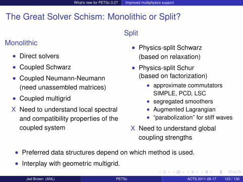
The Great Solver Schism: Monolithic or Split?
Monolithic
• Direct solvers
• Coupled Schwarz
• Coupled Neumann-Neumann(need unassembled matrices)
• Coupled multigrid
X Need to understand local spectraland compatibility properties of thecoupled system
Split
• Physics-split Schwarz(based on relaxation)
• Physics-split Schur(based on factorization)
• approximate commutatorsSIMPLE, PCD, LSC
• segregated smoothers• Augmented Lagrangian• “parabolization” for stiff waves
X Need to understand globalcoupling strengths
• Preferred data structures depend on which method is used.
• Interplay with geometric multigrid.
Jed Brown (ANL) PETSc ACTS 2011-08-17 123 / 130

What’s new for PETSc-3.2? Improved multiphysics support
Multi-physics coupling in PETSc
Momentum Pressure
• package each “physics”independently
• solve single-physics and coupledproblems
• semi-implicit and fully implicit
• reuse residual and Jacobianevaluation unmodified
• direct solvers, fieldsplit insidemultigrid, multigrid inside fieldsplitwithout recompilation
• use the best possible matrixformat for each physics(e.g. symmetric block size 3)
• matrix-free anywhere
• multiple levels of nestingJed Brown (ANL) PETSc ACTS 2011-08-17 124 / 130

What’s new for PETSc-3.2? Improved multiphysics support
Multi-physics coupling in PETSc
Momentum PressureStokes
Energy Geometry
Ice
Boundary Layer
Ocean
• package each “physics”independently
• solve single-physics and coupledproblems
• semi-implicit and fully implicit
• reuse residual and Jacobianevaluation unmodified
• direct solvers, fieldsplit insidemultigrid, multigrid inside fieldsplitwithout recompilation
• use the best possible matrixformat for each physics(e.g. symmetric block size 3)
• matrix-free anywhere
• multiple levels of nestingJed Brown (ANL) PETSc ACTS 2011-08-17 124 / 130

What’s new for PETSc-3.2? Improved multiphysics support
rank 0
rank 2
rank 1
rank 0
rank 1
rank 2
LocalToGlobalMapping
Monolithic Global Monolithic Local
Split Local
GetLocalSubMatrix()
Split Global
GetSubMatrix() / GetSubVector()
LocalToGlobal()
rank 0
rank 1
rank 2
Jed Brown (ANL) PETSc ACTS 2011-08-17 125 / 130

What’s new for PETSc-3.2? Improved multiphysics support
MatGetLocalSubMatrix(Mat A,IS rows,IS cols,Mat *B);
• Primarily for assembly• B is not guaranteed to implement MatMult• The communicator for B is not specified,
only safe to use non-collective ops (unless you check)
• IS represents an index set, includes a block size and communicator
• MatSetValuesBlockedLocal() is implemented
• MatNest returns nested submatrix, no-copy
• No-copy for Neumann-Neumann formats(unassembled across procs, e.g. BDDC, FETI-DP)
• Most other matrices return a lightweight proxy Mat• COMM_SELF• Values not copied, does not implement MatMult• Translates indices to the language of the parent matrix• Multiple levels of nesting are flattened
Jed Brown (ANL) PETSc ACTS 2011-08-17 126 / 130
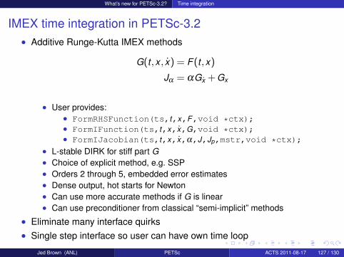
What’s new for PETSc-3.2? Time integration
IMEX time integration in PETSc-3.2• Additive Runge-Kutta IMEX methods
G(t,x , x) = F(t,x)
Jα = αGx + Gx
• User provides:• FormRHSFunction(ts,t,x,F,void *ctx);• FormIFunction(ts,t,x,x,G,void *ctx);• FormIJacobian(ts,t,x,x,α,J,Jp,mstr,void *ctx);
• L-stable DIRK for stiff part G• Choice of explicit method, e.g. SSP• Orders 2 through 5, embedded error estimates• Dense output, hot starts for Newton• Can use more accurate methods if G is linear• Can use preconditioner from classical “semi-implicit” methods
• Eliminate many interface quirks• Single step interface so user can have own time loop
Jed Brown (ANL) PETSc ACTS 2011-08-17 127 / 130
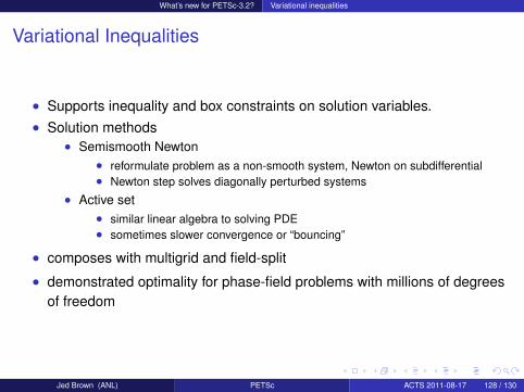
What’s new for PETSc-3.2? Variational inequalities
Variational Inequalities
• Supports inequality and box constraints on solution variables.• Solution methods
• Semismooth Newton• reformulate problem as a non-smooth system, Newton on subdifferential• Newton step solves diagonally perturbed systems
• Active set• similar linear algebra to solving PDE• sometimes slower convergence or “bouncing”
• composes with multigrid and field-split
• demonstrated optimality for phase-field problems with millions of degreesof freedom
Jed Brown (ANL) PETSc ACTS 2011-08-17 128 / 130

Conclusions
Conclusions
PETSc can help you
• solve algebraic and DAE problems in your application area
• rapidly develop efficient parallel code, can start from examples
• develop new solution methods and data structures
• debug and analyze performance• advice on software design, solution algorithms, and performance
• petsc-users,dev,[email protected]
You can help PETSc
• report bugs and inconsistencies, or if you think there is a better way
• tell us if the documentation is inconsistent or unclear
• consider developing new algebraic methods as plugins, contribute if youridea works
Jed Brown (ANL) PETSc ACTS 2011-08-17 129 / 130
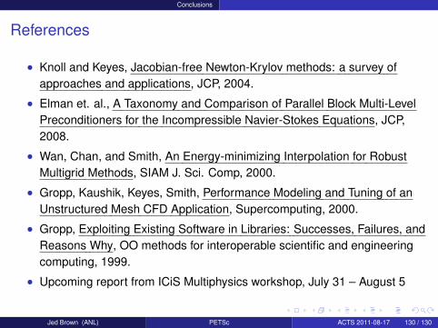
Conclusions
References
• Knoll and Keyes, Jacobian-free Newton-Krylov methods: a survey ofapproaches and applications, JCP, 2004.
• Elman et. al., A Taxonomy and Comparison of Parallel Block Multi-LevelPreconditioners for the Incompressible Navier-Stokes Equations, JCP,2008.
• Wan, Chan, and Smith, An Energy-minimizing Interpolation for RobustMultigrid Methods, SIAM J. Sci. Comp, 2000.
• Gropp, Kaushik, Keyes, Smith, Performance Modeling and Tuning of anUnstructured Mesh CFD Application, Supercomputing, 2000.
• Gropp, Exploiting Existing Software in Libraries: Successes, Failures, andReasons Why, OO methods for interoperable scientific and engineeringcomputing, 1999.
• Upcoming report from ICiS Multiphysics workshop, July 31 – August 5
Jed Brown (ANL) PETSc ACTS 2011-08-17 130 / 130


![Introduction to Scientific Computing · 2.1 Introduction to Scientific Computing Scientific computing – subject on crossroads of physics, chemistry, [social, engineering,...]](https://img.pdfslide.us/doc/110x75/5edc24c2ad6a402d6666af19/introduction-to-scientiic-computing-21-introduction-to-scientiic-computing.jpg)


![[MS-PEAP-Diff]: Protected Extensible Authentication ......Protected Extensible Authentication Protocol (PEAP)](https://img.pdfslide.us/doc/110x75/5f0eef6d7e708231d441aa24/ms-peap-diff-protected-extensible-authentication-protected-extensible.jpg)