THE POLITICS OF TAX ADMINISTRATION: EVIDENCE FROM SPAIN*

Alejandro Esteller-Moré (UB & IEB)

esteller@eco.ub.es

Abstract: Does there exist a connection between the political power and the tax administration? In this paper, we offer empirical evidence from Spain that there exists. First, the Spanish regional tax administration is not immune to the budgetary situation of the regional government, and tends to exert a greater (lower) effort in tax collection as the (expected) public deficit is greater (lower). At the same time, the system of unconditional grants provokes an “income effect” that disincentives the efforts carried out by the tax administration. Second, when the margin to lose a parliamentary seat in an electoral district decreases, the efforts also diminish, though this disincentive is lessened according to the parliamentary strength of the incumbent (evidence of electoral competition). JEL Code: H21, H72, H77

Address for correspondence: Alejandro Esteller-Moré

Institut d’Economia de Barcelona (IEB) Parc Científic de Barcelona

Edifici Florensa C/Adolf Florensa, s/n

08028-Barcelona (Spain) The author thanks Antonio Álvarez, Rafael Álvarez, Víctor Jiménez, Quique López, Francisco Pedraja, Alexandre Pedrós, Jaume Puig, José Raga, Javier Salinas, Albert Solé, and very specially Antoni Castells for the helpful comments received, though the usual disclaimer applies. Research support from SEC2000-0876 (Mº de Ciencia y Tecnología) and 2001SGR-30 (Generalitat de Catalunya) is gratefully acknowledged.

1

1. Introduction

There is no consensus in the relatively scarce literature on public finance and tax

administration about how the objective function of a tax administration should be

characterised (see Shoup, 1969, or Slemrod and Yitzhaki, 2000, for a recent review on

these issues). The most common way of characterising it is as a public agency that

maximises the amount of gross tax revenue collected1. However, several empirical papers

have suggested and shown that the efforts carried out by a tax administration are also

guided by electoral concerns (Toma and Toma, 1986; Hunter and Nelson, 1995; or more

recently, Young et al., 2001), and conditioned by the system of unconditional grants in the

case of the sub-central tax administrations (Jha et al., 1999; Baretti et al., 2002). In this

paper, we aim at testing several hypothesis concerning the political determinants of the

activities carried out by the regional tax administration in Spain.

First, we will check whether there exists a nexus between the tax administration and the

public budget, or instead the tax administration is simply a “black box” that -

independently of the “health” of the public finances, which are under the direct control of

politicians (i.e., the Ministry of Finances) - aims at obtaining as much tax revenue as

possible from the taxpayers2. That is, for instance, we will test whether the tax

administration exerts a greater effort when the (expected) public deficit is greater, and vice

versa. Second, we will analyse whether those efforts depend on the political strength of the

government and the electoral competitiveness in each electoral district (or province). Thus,

according to this hypothesis of “electoral competition”, we expect a lower effort in those

1 According to Slemrod and Yitzhaki (1987), this rule – that implies in equilibrium the equality between marginal cost and marginal benefit - will not be optimal, since while the marginal cost is a real cost, the marginal revenue is simply a transfer from the taxpayer to the tax administration. That objective function would only be optimal as long as the tax administration operates given a level of inputs (Andreoni et al., 1998; Slemrod and Yitzhaki, 2000). 2 In this sense, the spirit of our analysis is very close to Toma and Toma (1986)’s framework, in which "... the tax rates [emerge],..., as a consequence of competition among political actors in the legislative arena. Once this structure has been established, a separate government body, the treasury, will devote resources toward the collection of revenue. The question of relevance then becomes how treasury bureaucrats will vary their collection activity in response to changes in the legislative determined tax rate" (pp. 141-142). However, in Toma and Toma, the reaction is only caused by the variation in the statutory tax parameters, while we consider any source of budgetary shock (e.g., an increase in the cost or the demand of provision of public goods); and the influence of the politicians on the bureaucrats is only due to an appropriation process by the latter, while we do not make explicit the source of connection between both actors.

2

electoral districts where the margin for winning or losing a parliamentary seat is smaller,

though a priori such incentive should be lower the greater the parliamentary strength of the

incumbent (e.g., measured through the percentage of seats in the regional parliament)3.

The empirical validation of any one of those two hypothesis would confirm the connection

between the tax administration and the political power, though they both embody totally

different normative implications. In the first case, the tax administration becomes an extra

tax instrument for the government - apart from the statutory tax parameters - in order to

obtain additional tax revenues (and so meet the constituency expenditure needs), which

must produce a greater global efficiency of the tax system (Slemrod, 1990). In the second

case, on the contrary, there would be a lower level of global efficiency (and of inter-

provincial equity), since the efforts carried out by the tax administration are simply guided

by electoral motives.

In order to test such hypothesis, we will perform an empirical analysis based on the

estimation of stochastic frontiers (Aigner et al., 1977; Meeusen and van den Broeck, 1977).

From the estimation of a tax revenue function, we will obtain a frontier function. The fact

that certain observations lie below the frontier can be due either to an estimation error or to

inefficiency (i.e., lower efforts in tax administration). This technique disentangles both

effects. Given this, we will be interested in identifying which factors explain the distance

of each decision unit to the frontier (this is the so-called inefficiency effects model). The

methodology developed by Battese and Coelli (1995) applied to a panel of data will permit

3 Among other studies that have tested the importance of the marginal “electoral productivity” by district in the “design” of public policies, see Wallis (1996), for the distribution of federal grants to the US states; Case (2001), who tests the political criteria that guide the allocation of block grants from federal to sub-federal levels of government in Albania; Castells and Solé-Ollé (2002), for the allocation of national investment across Spanish regions; Garrett and Sobel (2002), who test the presidential influence on the rate of disaster declaration and the allocation of emergency funds across US states; Besley and Burgess (2002), Besley and Case (2002), or Besley and Preston (2002), all papers showing that the responsiveness of the government is greater the greater the electoral competition; or Young et al. (2001) - already cited in the main text – who test whether the tax audit probability by district depends on the electoral importance of that district to the president. Certainly, all these studies show the importance of the electoral motives for the design of public policies, though the measurement of “political competition” differs in each case according to the system of election of the regional representatives in the national assembly. This will have to be appropriately dealt with in our analysis, given the multi-party system prevailing in Spain (e.g., different to the US system, where most of the cited studies have been applied), and the functioning of the d’Hondt formula to transform the votes obtained in a district into seats in the national parliament.

3

us to carry out such identification. In fact, this methodology has already been applied by

other papers to study the behaviour of the tax administration (Jha et al., 1999; and

Maekawa and Atoda, 2001).

Our empirical analysis will be based on the behaviour of the Spanish tax administration at

the regional level (in Spanish, Comunidades Autónomas, CCAA). Nevertheless, in order to

enlarge the database, each province (or in political terminology, electoral district) of a CA

will be considered as a decision unit in the analysis. In Spain, the CCAA have the power to

administer certain taxes ceded by the central government since the beginning of the 80’s,

while the tax autonomy to vary their statutory tax parameters has been null, at least until

1997. This will be the institutional context that we will have to deal with. Interestingly

enough, this context will permit us to test to what extent the relative importance of the

unconditional grants in the regional budgets influences the efficiency in tax administration

(in our case, exclusively through an “income effect”), like Jha et al. (1999) and Baretti et

al. (2002) have shown for India and Germany, respectively.

The results obtained from our analysis point out in the direction of a close connection

between the political power and the tax administration. Thus, first, we find that the level of

efficiency (i.e., the effort in collecting taxes) tends to be greater, the greater the level of

(expected) public deficit. However, if the level of unconditional grants from the central

government is high enough (approximately, 41% with respect to public expenditure, above

the average during the period of analysis), efficiency diminishes. Second, the tax

administration is also guided by electoral concerns, since tends to decrease its level of

efficiency (with the aim of increasing the level of popularity of the incumbent) when the

margin for losing a parliamentary seat is low, while this decrease is lower the higher is the

political strength of the incumbent in the regional parliament. Both results are quite robust

to different specifications of the model as we will show.

The remainder of the paper is organised as follows. In the next section, we set up the basic

hypothesis concerning the empirical analysis, first, with respect to the tax revenue function

and, second, with respect to the determinants of the efforts in tax administration. In the

third section, we will describe the empirical methodology and the database constructed for

the analysis. In section four, we will present the results of the empirical estimation, while

section five contains some concluding remarks.

4

2. Tax Administration and Politics

2.1. The tax revenue technology

In this section, we will define the tax technology, since it will permit us to identify the

motives that guide the efforts of the tax administration. The tax technology - which will be

later estimated in the empirical analysis - is a function that translates the inputs of the tax

administration (basically, number of tax inspectors and general staff, on the one hand, and

stock of capital, on the other), I, the (marginal) statutory tax rate, t, and the tax capacity, B,

into the tax revenue collected, T (Mayshar, 1991). However, given the value of that

variables, not all the potential revenue will presumably be collected, given the presence of

tax avoidance and/or evasion4, S, such that 01 ≥≥ S . Therefore, the tax technology is a

function T(I,t,B,S). The main differences with the function originally proposed by Mayshar

is that, on the one hand, we have distinguished between the inputs of the tax administration

and the statutory tax rate, while he includes both factors into just one variable, θ . On the

other hand, Mayshar names S as “tax-shielding activity”, though he himself shows that it

can also be interpreted as the level of tax evasion (Mayshar, 1991, fn. 5).

The literature has identified several factors that might explain tax evasion. Following

Andreoni et al. (1998), these can be mainly classified into three groups: (i) income and tax

rates; (ii) demographic and social factors; and (iii) penalties and audit probabilities.

Nevertheless, the expected sign of each one of these variables is not clear-cut, since the

results of the theoretical and empirical models do not always coincide (see Andreoni et al.,

1998, pp. 838-47, for a detailed discussion on these issues). The classical theoretical

models of tax evasion (Allingham and Sandmo, 1972) predict that the greater the audit

probability, the lower the level of tax evasion, which will also happen in the case of a

greater penalty. The same result is obtained with respect to income as long as the taxpayer

exhibits decreasing risk aversion with respect to income. Finally, the effect of an increase

in the (marginal) tax rate is not obvious, since it depends on an “income effect” (in favour

of less tax evasion) and on a “substitution effect” (that promotes less tax compliance).

However, if the penalty is proportional to the amount of tax evaded, the “substitution”

4 See, e.g., Slemrod and Yitzhaki (2000) for an extensive explanation of the definitions of each one of those two concepts, though they both have the same consequence: a reduction in the potential amount of tax revenue collected.

5

effect disappears, and so an increase in t always promotes more tax compliance (Yitzhaki,

1974). Due to the multiplicity of factors that might exert some influence on the decision to

evade taxes, the empirical (and experimental) analysis have also included socio-economic

variables like the level of education, the age, the race or the occupation of the taxpayer (see

Andreoni et al., 1998, pp. 840-1).

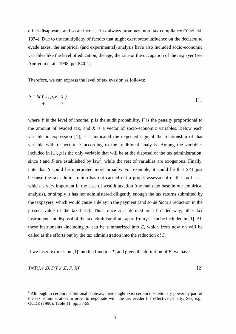
Therefore, we can express the level of tax evasion as follows:

? - - - )X ,F ,p ,t ,Y(SS

+=

[1]

where Y is the level of income, p is the audit probability, F is the penalty proportional to

the amount of evaded tax, and X is a vector of socio-economic variables. Below each

variable in expression [1], it is indicated the expected sign of the relationship of that

variable with respect to S according to the traditional analysis. Among the variables

included in [1], p is the only variable that will be at the disposal of the tax administration,

since t and F are established by law5, while the rest of variables are exogenous. Finally,

note that S could be interpreted more broadly. For example, it could be that S<1 just

because the tax administration has not carried out a proper assessment of the tax bases,

which is very important in the case of wealth taxation (the main tax base in our empirical

analysis), or simply it has not administered diligently enough the tax returns submitted by

the taxpayers, which would cause a delay in the payment (and so de facto a reduction in the

present value of the tax base). Thus, once S is defined in a broader way, other tax

instruments at disposal of the tax administration - apart from p - can be included in [1]. All

these instruments -including p- can be summarized into E, which from now on will be

called as the efforts put by the tax administration into the reduction of S.

If we insert expression [1] into the function T, and given the definition of E, we have:

T=T(I, t ,B, S(Y ,t ,E, F, X)) [2]

5 Although in certain institutional contexts, there might exist certain discretionary power by part of the tax administration in order to negotiate with the tax evader the effective penalty. See, e.g., OCDE (1990), Table 11, pp. 57-59.

6

Defined in this way, the tax technology shows a third difference with respect to the original

model of Mayshar (1991). In his model, he does not explicitly differentiate between I and

the variables at disposal of the tax administration, E. However, in our paper, such

difference becomes crucial to understand our empirical framework. Such difference

becomes clear if we suppose that the problem of collecting tax revenue consists of two

steps (see Andreoni et al., 1998, pp. 826-827):

1st. A social planner chooses all relevant policy parameters (including the statutory tax

rate) and the audit budget, or more generally, the tax administration budget (which

includes the number of personnel and the stock of capital at disposal of the tax

administration). Therefore, the social planner has chosen t and I, but also F (see fn. 5).

2nd. The tax administration is delegated the responsibility to enforce the tax obligations

through a diligent administration of the tax returns, the realisation of tax audits or the

proper assessment of the tax bases, among other tasks. Hence, the tax administration, given

the budget at its disposal, chooses E (being this variable difficult to measure or to concrete

into one single measure given the wide range of actions that can be carried out by a tax

administration as we have justified).

Precisely, it is important to bear in mind that the main aim of the paper is finding the

variables that explain the behaviour of the tax administration, i.e., those variables that

guide the selection of E. According to the empirical methodology - which will be

explained in detail in section 3.1. - we will (consistently) estimate both T and S. Then,

given the supposedly positive relationship between S and E (e.g., higher p) and given the

rest of variables included in [1], as long as we find a positive relationship between the

potentially explanatory variables of E, on the one hand, and S, on the other, we will have

indirectly shown the influence of the former group of variables on the choice of E6. That is

why, it is crucial for our empirical analysis to set up certain basic hypothesis concerning

6 E.g., this approach has also been followed by Grossman et al. (1999) in estimating the efficiency of US local governments in "producing" local property value, also employing the methodology proposed by Battese and Coelli. Thus, the authors state that "... such deviations from the maximum value are affected by local governance decisions; these in turn are affected by observable characteristics regarding the level of competition faced by the city and its policymakers" (p. 281). In our case, the “deviations from the maximum value” corresponds to S, while those "observable characteristics" are precisely those included as explanatory variables of S.

7

the choice of E.

2.2. The determinants of the efforts in tax administration

All the variables that we will identify as potentially explanatory of S are qualified as

political in the sense that (i) they are connected with the “health” or composition of the

public budget (from now on, budget connection), which responsibility is at hands of a

political responsible, or (ii) the tax administration is used in order to gain electoral

popularity by the incumbent (electoral competition), or finally, (iii) the government exerts

its influence on the tax administration in order to impose its partisan preferences in the

intensity put into tax collection (partisan preferences).

The hypothesis concerning each one of these three groups of factors that could potentially

affect the choice of E are the following:

(i) Budget connection. In the empirical analysis, we will test two different hypothesis with

respect to the budget connection:

(i.1) First, we will test whether the government conditions the efforts carried out by the

tax administration according to the “health” of the public finances. That is, in front

of a negative (positive) shock in the public finances, does the tax administration –

induced somehow by the political power- react increasing (reducing) its efforts in

collecting taxes? Note that the negative (positive) shock could be due either to a

demand of the citizens in favour of a higher (lower) level of public goods7 or,

alternatively, to a decrease (increase) in the level of tax bases, maintaining the

statutory tax rates, or to a reduction (increase) of the latter established in the annual

budget, maintaining the level of tax bases8, or to a combination of all these causes.

In order to test this hypothesis, we will use the (expected) public deficit at the

beginning of the fiscal year as explanatory variable, and so it will not be possible to

discern the cause(s) that has (or have) provoked the financial needs (or surplus).

7 See Dušek (2002), who very appropriately calls this effect as a "demand effect" in the process of tax revenue collection, different from a "technological shock" in the process of generating revenue, or from a "political effect" produced as a response to the "technological shock". 8 See Toma and Toma (1986).

8

(i.2) Second, it might be the case that not only the “health” of the public finances affect

the efforts of the tax administration, but also the composition of the public budget.

In this sense, we will test whether the relative importance of the amount of

unconditional grants received by a region from the central government provokes an

“income effect” that lowers the marginal value of any additional tax revenue

collected up to the extent to make unbeneficial carrying out any additional (costly)

effort by the tax administration (see Jha et al., 1999, for India; and Baretti et al.,

2002, for Germany, who are also able to detect a "substitution effect" that in

addition to the “income effect” disincentives the efforts in tax administration).

(ii) Electoral competition. It is usually believed that tighter races for political office force

the incumbent to be more responsive to constituency needs, due to the higher risk of

political defeat9. Thus, as long as voters dislike the burden of taxes, in order to minimise

the risk of defeat in an electoral district (plurality system) or of losing a parliamentary seat

assigned to a district (proportional system), the political power, through the tax

administration, will be induced to reduce the efforts in collecting taxes in that district.

Then, the key question to test this hypothesis is how to measure “electoral competition”

(see for a review Holbrook and van Dunk, 1993, and their proposed index of measurement

instead of the “Ranney index”, the most commonly used)10. All of the measures proposed

in the literature are based on the assumption that political parties look at past electoral

results to get an idea of how tight the next election contest will be. However, it is self-

evident that the way of measuring “electoral competition” depends on the electoral system.

In Spain, the selection of the regional representatives in the lower house is done according

to a proportional system, in which the Hondt’s Law is used to transform provincial votes

into seats in the regional assembly11. Hence, in order to measure the electoral competition

in an electoral district, the most natural way of doing it is calculating the minimum number

of votes the incumbent should lose (win) in order to lose (obtain) one seat in the regional

9 Among many others, see on this issue Holbrook and van Dunk (1993), Besley and Case (2002), and the references cited therein. 10 Besley and Case (2002), p.23, recognise that "there is no unanimously agreed method of measuring this ["political competition"]". 11 For an introduction to the Spanish electoral system, see Astorkia (1998).

9

parliament (see the Annex for a description of this calculus). The lower the margin, the

higher the electoral “district competition”. Nevertheless, such marginal lose (win) will be

relevant to the incumbent depending on her strength in the regional parliament. That is,

e.g., if the margin to lose a seat in a certain electoral district is very low, but the

government disposes of a “comfortable” majority in the regional parliament, such lose will

be less important than in the case that such seat is crucial to obtain a majority in the

parliament. On the whole, we propose to estimate “electoral competition” as follows:

Powerary Parliament* nCompetitio DistrictnCompetitio Electoral

−+= [3]

Therefore, the measure of “electoral competition” is a combination of two factors, which

tend to vanish with each other. Later on, in the empirical section, we will test other

measures of “electoral competition”, though in any case they all will be based on [3].

(iii) Partisan preferences. Given that the efforts in tax administration end up by affecting

the effective tax burden borne by the citizens, it seems reasonable to assume that the

governments – as long as they are connected with the tax administration, and given that the

statutory tax parameters have already been established - will condition such efforts in

order to determine the final weight of the public sector in the economy. As usual, if we

distinguish between “leftist” and “rightist” governments, it is expected that the former tend

to exert a relatively higher level of effort in tax administration, and so obtain a higher level

of tax revenues (see Franzese, 2002, for a recent and complete review on the main theories

and empirical results concerning the partisan motivations of the governments).

3. Empirical methodology and data

3.1. Empirical methodology

The methodology that we will employ to estimate [2] is based on Battese and Coelli

(1995)12. This methodology permits estimating a stochastic frontier of tax revenue, i.e. the

maximum amount of tax revenues that could be collected given, in our case, the (marginal)

12 See also Coelli et al. (1997).

10

statutory tax rate, t, the tax capacity, B, and the administrative inputs, I. The error term

obtained from this estimation is decomposed into two parts: one is the error term of the

econometric specification, and the other one is the so-called (technical) inefficiency effect.

That is, the technical inefficiency is the difference between the observation of a decision

unit and the frontier. Crucially, in our case, the “inefficiency effect” is directly related with

S, as we have shown in section 2.1, and so we will explain it according to the hypothesis

set up in section 2.213.

The estimated frontier is stochastic, since we allow that a decision unit is out of the frontier

either due to a random shock or to an error of measurement. Instead, the deterministic

techniques do not permit to distinguish between those two components, so biased measures

of technical efficiency are usually obtained. Moreover, Battese and Coelli’s methodology

permits to overcome the inconsistency that arises when one tries to explain inefficiency

through methods of estimation in two steps.

Briefly, Battese and Coelli (1995)'s methodology proposes to estimate the following

function for a panel of data14:

( )itititit UVxexpT −+= β ,

where itT is the amount of tax revenue collected by the tax administration i in the period t;

itx is a vector of (k*1) values of inputs (in our case, tax capacity and administrative inputs,

and the statutory tax rate) and other explanatory variables associated to the unit i in the

period t;

13 In fact, though throughout the paper we will not distinguish between tax evasion (S) and technical efficiency, both measures are not fully identical. The reason is that technical efficiency is measuring the relative performance of the tax administrations in closing the gap between the maximum amount of tax revenue that could be collected and the tax revenue collected, given a level of tax capacity, administrative inputs and statutory tax parameters. Therefore, it could be the case that all tax administration were performing equally bad (or that the level of the tax administration budget were still low, given its productivity), and all the levels of efficiency – as they are obtained from the comparison of the observed performances - were close to 100%. In conclusion, other measures should be employed in order to obtain the absolute levels of tax evasion (see for such measures, e.g., Slemrod and Yitzhaki, 2000, pp. 21-23). 14 The joint estimation of the stochastic tax revenue frontier and the explanatory equation of the inefficiency effects will be performed with the software FRONTIER V. 4.1, Coelli (1996).

11

β is a vector of (k*1) unknown values to be estimated;

itV are assumed to be stochastic errors identically and independently distributed, with a

normal distribution with zero average and an unknown variance, Vσ ;

itU are non-negative random variables, associated with technical inefficiency, they are

assumed to be independently distributed, in such a way that itU is obtained by truncation

(at zero) the normal distribution with mean δitz , and variance, 2σ ;

itz is a vector of (1*m) explanatory variables associated to the inefficiency of the decision

unit along time, among which those variables identified in section 2.2. as potentially

explanatory of the efforts carried out in the collection of taxes will be included; and,

finally, δ is a vector of (1*m) unknown coefficients, to be estimated.

Therefore, from the previous assumptions, technical inefficiency (i.e., S) can be specified

in the following way:

ititit WzU += δ , where the random variable itW is defined by truncation of the normal

distribution, ),o(N 2σ , at δitz− , that is, δitit zW −≥ .

By means of the definition of γ (Battese and Corra, 1977), such that )( vuu222 σσσγ +=

and 10 ≤≤ γ , it is possible to discern the relative importance of the inefficiency effects

versus the estimation error of the stochastic frontier. Hence, e.g., if 0=γ , the observed

deviations from the frontier are exclusively due to an error of estimation, and the

explanatory variables included in the inefficiency effects model should be included in the

estimation of the stochastic frontier, and a traditional panel data analysis is the adequate

econometric technique instead of the stochastic frontier models15.

15 The value of γ is obtained through the resolution of an iterative process, like the one generated by the Davidon-Fletcher-Powell’s algorithm. Thus, given an initial value (where, with the exception of 0β and σ , the estimates by OLS of β are employed), the iteration process is solved for that value of γ that maximises the likelihood-function (Coelli, 1996, pp. 11-12).

12

In the estimation of the stochastic frontier, we will also include a set of fixed and time

effects. The fixed effects aim at picking up certain structural factors concerning the tax

capacity of a decision unit or institutional factors that condition the composition of the

administrative inputs, I16. As long as such structural or institutional factors were correlated

with I, the exclusion of the fixed effects would cause inconsistent measures of the

s'β (Mundlak, 1961). With respect to the time effects, they have been included to control

for common changes in the statutory tax rates along the period of analysis, since as we

have already said, during this period there have not been differences among CCAA in the

setting of the statutory tax rates, though since 1997, the CCAA have gained an increasing

tax autonomy. The time effects also control for the existence of common macroeconomic

shocks that could have affected the tax capacity of all the decision units, and which had not

been precisely captured by the variables that already measure the tax capacity.

In order to control for the effect of the statutory tax rates on S, we have also included a set

of time effects in the equation of the "inefficiency effects model". Moreover, given that

one potentially explanatory variable of the inefficiency is the (expected) public deficit (see

section 2.2., point (i.1)), the time effects could also help to alleviate the likely endogeneity

of the (expected) public deficit. Thus, we have not employed the public deficit as

explanatory variable, since the simultaneous relation is obvious: ceteris paribus, the

greater the inefficiency, the greater the public deficit, while we precisely want to test the

reverse causality. However, having included instead the (expected) public deficit, there

could still exist a simultaneous relationship if the budgetary decisions and the decisions

about the efforts of the tax administration are simultaneously adopted - which does not

seem too much realistic- or both decisions are affected by the economic cycle (the

expected deficit is negatively affected by the downturn phase of the cycle, but it might also

be more difficult to collect tax revenue at that moment; see for a possible justification of

this argument, Andreoni, 1992). In this latter case, the inclusion of the time effects

becomes an useful instrument for controlling that potential source of simultaneity bias.

Finally, we have to say that the structure of our stochastic frontier is very similar to Hunter

and Nelson (1996), since they only include inputs in the way we have defined I (personnel

16 Usually, in the literature on technical efficiency estimation, the fixed effects are also interpreted as a "management index".

13

and capital stock), though they treat the tax revenue collected from the audit processes as

the only output of a tax administration. However, in order to perform an analysis of

efficiency, as we will do, it is difficult then to evaluate the relative efficiency of each

decision unit, unless the researcher has very precisely controlled for the voluntary

compliance of the taxpayers. Otherwise, it could be the case that a decision unit has not

obtained any flow of revenue from the tax audit processes, and in consequence were

negatively evaluated, while voluntary compliance was close to 100%.

3.2. Data

Most of the data employed in the analysis have been obtained from the information that

annually appears in the National Budget (Presupuestos Generales del Estado, PGE) as an

Annex, under the title "Report on the cession of taxes to the Autonomous Communities".

The realization of these reports is obliged by the Act 14/1996, 30th December, which

regulates the cession of taxes from the central government to the CCAA17. In particular,

the information that we have obtained form such reports has been the following:

• Tax revenue collected from the taxes administered by each CA: Net Wealth Tax; Wealth

Transmission Tax (intervivos and mortis causa); a tax on certain business operations

("Impuesto sobre Transmisiones Patrimoniales y Actos Jurídicos Documentados"); and

taxes on gambling (except Baleares and Cantabria, to which such competence has not been

transferred18). During the period of analysis, these taxes have represented around the 12%

of all the budgetary revenues of the CCAA. Table 1 shows the relative importance of each

one of these taxes. The amount of collected tax revenue corresponds to effective collected

tax revenue, not provisional or forecasted, and includes both the revenue collected through

the own offices of the CA ("oficinas gestoras") and through offices that do not directly

depend on each CA ("oficinas liquidadoras"). From now on, we will name this latter type

of offices as "external offices".

17 The taxes administered by the CCAA are so-called "ceded", since they originally belong to the central government, but they were ceded to the CCAA (the first cession occurred in 1982, for Catalonia). However, though the CCAA are entitled to maintain all the collected tax revenues, until 1997 they were not entitled to perform tax reforms on this set of taxes. 18 Therefore, this is a typical institutional factor that must be controlled for by the fixed effects.

14

[INSERT TABLE 1]

• Inputs of the Tax Administration: number of personnel (tax inspectors and the rest); stock

of computers; and m2 of offices exclusively dedicated to the tasks of tax administration.

• Explanatory variables of the inefficiency of the Tax Administration: percentage of returns

submitted through the "external offices"; and concentration of tax bases (calculated as the

total amount of collected tax revenue divided by the total number of tax returns, excluding

the taxes on gambling). In the first case, this variable has been included in order to control

for this institutional factor that might affect the level of efficiency, without any previous

expectancy about its sign. In any case, there exists the suspect that the great mobility of the

responsibles of those "external offices" and their low incentives to collect tax revenue

might cause some inefficiency in the process of tax collection. In the second case, we

expect that the greater the concentration of tax bases (in the way it has been measured), the

greater the level of efficiency, since we would expect a greater profitability by tax return of

a marginal effort of the tax administration.

The reports present a delay of two years, that is, for instance, in the budget of the year

2000, there appeared the report of the fiscal year 1998. The reports employed to construct

our database have been those that correspond to the years 2000 (1998), 1999 (1997), 1998

(1996), 1997 (1995) and 1994 (1992). Thus, the analysis consists of 225 observations

(since 45 provinces have been included in the database, and Madrid has been excluded

from the analysis, since it has only very recently started to administer its ceded taxes, and

still does not administer the Net Wealth Tax).

The rest of variables have been obtained from the following statistic sources:

• Gross Domestic Product (GDP), Capitalisation of the returns of capital (W): from

National Income of Spain and its provincial distribution (Volume II), BBV, for all the

years. As there do not exist official statistics about the wealth of a region/province (apart

from the real-state property, the so-called "valor catastral", VC, which is measured by a

National Agency), an approximation to the wealth of each province has been calculated

through the capitalisation of the provincial returns on capital according to the national

15

interest rate of the corresponding year (source: Bank of Spain).

• Amount of unconditional transfers received by the CA as a percentage of total

expenditure: this amount of funds is composed by a share based on expenditure needs in

the total amount of National tax revenue ("Participación en los Impuestos del Estado",

PIE), and a territorial share in the personal income tax (since 1995), being both sources of

tax revenues collected by the central government. This information has been obtained from

the Informe Económico-Financiero de las Administraciones Territoriales, several years,

Ministry of Public Administrations.

• Public deficit: the public deficit has been calculated as a percentage of the regional GDP,

and it is the expected deficit that appears in the regional budget at the beginning of the

fiscal year. This information has also been obtained from the Informe Económico-

Financiero de las Administraciones Territoriales, op. cit.

• Political variables: from the Anuario de El País, several years, we have differentiated

through a dummy variable between the regional leftist governments (=1) from the rightist

ones (=0); also from this source, all the data necessary to construct the variable “political

competition” have been obtained (see Annex).

All the monetary magnitudes have been transformed into constant prices of the year 1995

through the national index of consumer prices (National Institute of Statistics, INE). Table

2 provides some descriptive statistics of all the data.

[INSERT TABLE 2]

Apart from the political variables of section 2.2. that aim at explaining E, the GDP p.c. in

order to control for its supposedly positive relationship with S according to the traditional

theoretical models of tax evasion (see section 2.1), the "concentration of tax bases", the

percentage of tax returns submitted through the "external offices", and the time effects, no

other variable has been included in the inefficiency effects model. But according to

expression [1], we could have also included some "socio-economic variables". However,

given that, on the one hand, the ceded taxes do not affect all the citizenship (e.g., the

16

transmission of wealth is clearly a non-periodical tax, while the wealth tax only affects

very rich people), the inclusion of socio-economic variables (like the level of education or

age) might have given a misleading picture of the group of taxpayers. On the other hand,

that group of variables might be correlated with the (expected) public deficit, as long as

they measure expenditure needs, while other type of variables like the composition of the

tax bases (e.g., percentage of the tax bases that are financial capital or real state property)

are not available. In any case, we believe that the exclusion of that variables will not bias

the estimates of the rest of variables as long as we do not expect a serious correlation of the

variables included with those omitted.

4. Empirical results

4.1. Basic Results

The results of the basic econometric estimations are reported in Table 3. The most

complete specification is Model 3, in which we have included both administrative and tax

capacity inputs - interacted with a time trend and without interaction - and all the

potentially explanatory variables of the inefficiency effects. The estimates of Model 3

suggest that the only administrative input that positively contributes to increase the amount

of collected tax revenue is the number of tax inspectors, though with a very low elasticity

(1,5%). With respect to the inputs of tax capacity, those picking up the level of wealth (W

and VC) are only significant when they are interacted with a time trend, while the impact

of GDP is significant with and without such interaction. In order to check the empirical

relevance of other alternative specifications of the stochastic frontier, in Model 1 we test

the hypothesis that the inclusion of the administrative inputs can be rejected, which result

is negative. In Model 2, the significance of the interaction of all the inputs with a time

trend is tested, and the result is again negative. In Table 4, there appear the Generalized

Likelihood-Ratio Tests carried out confronting Model 3 with Model 1 and Model 2, and

also testing the inclusion of the time and fixed effects in Model 3, which is accepted. Thus,

the specification of the stochastic frontier in Model 3 seems to be robust to alternative

specifications.

[INSERT TABLE 3]

17

[INSERT TABLE 4]

Then, following with the estimates obtained in Model 3, with respect to the inefficiency

effects model, the percentage of tax returns administered in “external offices” clearly

increases the inefficiency of the tax administration. As expected, the greater the

concentration of tax revenue in less tax returns, the lower the level of inefficiency. It was

also expected that a greater level of income p.c. (measured by the GDP) implies a greater

level of inefficiency, given the normally supposed positive relation between income and

tax evasion, though in Model 3 this estimate is not statistically different from zero19. With

respect to the political variables, first, the estimates suggest a powerful connection between

the public budget and the tax administration (being all the estimates statistically

significant): as long as the relative importance of the unconditional grants in the regional

budget is greater than 31,71%, the efforts in tax administration tend to diminish; while

when the (expected) public deficit is greater than 1,55%, the efforts tend to increase.

Second, the alignment of the tax administration with the electoral concerns of the

incumbent is less obvious, since the latter only distorts the efforts of the former depending

on the narrowness of the margin to lose a parliamentary seat, though this influence is

lowered according to the strength of the incumbent in the regional parliament (measured as

the percentage of parliamentary seats). Hence, when the margin to lose a parliamentary

seat has diminished in a certain electoral district (in the latest electoral contest), the tax

administration tends to diminish its efforts in collecting taxes in that district, though this

disincentive disappears when the percentage of parliamentary seats hold by the incumbent

is greater than 52,50%. Curiously enough the impact of the “political competition” on the

efforts carried out by the tax administration does not hold with respect to the margin of

wining a parliamentary seat20. Finally, there is also some evidence of partisan preferences,

19 Note that this variable – in conjunction with the (expected) public deficit – could also be picking up a “demand effect”. 20 We tried alternative definitions of “district competition”, which were always rejected by the better performance of the one that appears in Table 3. For example, instead of including the margin for losing or wining a parliamentary seat in absolute values, we included it as a percentage, or chose the smallest one between the margin for losing and the margin for wining a parliamentary seat. Finally, we also tested the possibility of a electoral cycle (assigning a dummy equal to one for the electoral year, or even trying it for the electoral year and the year before), and interacted it with the margin for losing and wining a parliamentary seat. However, these hypotheses were rejected as well.

18

in the sense that leftist governments tend to exert a relatively lower effort in tax

administration21.

In order to check the robustness of the results obtained from Model 3, in Model 4 we have

omitted all the statistically insignificant variables according to the Generalized Likelihood-

Ratio Test (see again Table 4). In the inefficiency effects model, only the exclusion of the

variable “Left” and of those variables related with the margin of wining a parliamentary

seat has been accepted, while none of the inputs included in the stochastic frontiers have

been excluded. In Model 4, not only the tax inspectors contribute to increase the amount of

taxes collected, but also the general staff. Thus, the elasticity of all the staff is 11,10%

(invariable along time). The elasticity of the capital stock of the tax administration in terms

of square meters of offices is negative and also invariable along time (-5,20%), while the

elasticity of the number of computers is not statistically significant from zero, though its

inclusion in Model 4 cannot be rejected22. The elasticity of the inputs of tax capacity is

(slightly) variable along time and, for example, for t=5, this elasticity is 110,40%.

With respect to the variables included in the inefficiency effects model, the signs of the

estimates do not vary from Model 3, and so the previous conclusions still apply. However,

the thresholds of the political variables have slightly varied. In Model 4, the percentage of

parliamentary seats that eliminates the disincentives of the tax administration in the case

that the margin to lose a parliamentary seat has narrowed in a electoral district is 53,27%

(slightly greater than in Model 3). Now the (expected) level of public deficit has to be as

high as 1,64% (during the period, its average has been 0,57%) in order to incite the tax

administration to exert a higher level of effort, while the relative importance of the

unconditional grants has to be greater than 40,84% (higher than in Model 3) in order an

“income effect” disincentives the efforts in collecting taxes.

Finally, in Table 5, there appears the ranking of efficiency by province and year obtained

from Model 4. The average of efficiency during the period is 83,77%, though the level of

21 In a preliminary version of a paper by Besley and Preston (2002), p. 16, they find that "labour parties" tend to collect a relatively lower percentage of tax revenues (being this, according to their model, a measure of political accountability). 22 Cfr. Hunter and Nelson (1996), p. 112, who also find negative estimates of the variables included in the production frontier of the tax administration.

19

efficiency tends to vary across the period, having reached its maximum in 1992 (86,76%)

and the minimum in 1998 (80,77%). From the ranking, it is also particularly remarkable

the poor performance of Teruel (Aragón), which not only always remains in the last

position of the ranking, but also presents a very bad performance in absolute values, being

its maximum level of efficiency 47,57% in 1997.

[INSERT TABLE 5]

4.2. Additional Results

Apart from the percentage of parliamentary seats, we have tried other alternatives to the

measurement of the parliamentary strength of the incumbent. The results – only of the

inefficiency effects model - are shown in Table 6. In particular, we have tried two

alternatives: first, in Model 5 the parliamentary strength has been measured through the

difference between the number of seats hold by the incumbent and the main party of the

opposition (in percentage, though the results do not differ very much if such difference is

measured in absolute values). Second, in Model 6, the parliamentary strength is picked up

by a dummy variable, which value is 1 in the case that the incumbent holds a majority in

the regional parliament (>50% of seats), and 0 otherwise. From Table 6, it can be

appreciated that the main results obtained from Model 3 do not vary. That is, the tax

administration only becomes an important electoral instrument for the incumbent as long

as the margin of votes for losing a parliamentary seat in a certain electoral district has

shrunk. Thus, for instance, if the incumbent holds a majority of seats (Model 6), such

effect almost fully vanishes. However, it seems that the parliamentary strength is not so

accurately measured if we just consider the distance with the main party in the opposition,

since in that case the estimates are only significant at the 10% level (see Model 5). Both in

Model 5 and Model 6, neither the sign nor the magnitude of the rest of estimates

substantially change.

In Model 7, the parliamentary strength of the incumbent is included without interaction.

Although the variable has the expected sign – the greater the parliamentary strength, the

more secure is the incumbent in power, and so the greater effort carries out in collecting

taxes all over the region – it is not statistically different from zero, and its inclusion is

rejected according to the Generalized Likelihood-Ratio Test (see Table 7).

20

[INSERT TABLE 6]

In Table 7, we present the tests carried out in order to check the empirical relevance of

each one of the alternative hypothesis regarding parliamentary strength. In the table, each

one of the alternative definitions of parliamentary strength described above is indicated by

φ . Leaving aside Model 7, since Model 3 is clearly preferred to it, only in Model 5 the

inclusion of all the variables relating to the political competition is rejected.

[INSERT TABLE 7]

5. Conclusions

This paper has empirically analysed the behaviour of the Spanish regional tax

administration. In particular, it has shown the close connection between the political power

and the tax administration itself. Such connection implies that, on the one hand, the tax

administration reacts to the budgetary situation of the regional government. On the other

hand, the incumbent also takes advantage of the tax administration in order to gain

electoral popularity in those electoral districts where the margin to lose a parliamentary

seat is small, though at a decreasing rate according to its strength in the regional

parliament. The empirical relevance of both results has been shown from the estimation of

a stochastic frontier tax revenue function following the methodology proposed by Battese

and Coelli (1995) for panel data.

As we already stated in the introduction, the normative implication of each one of those

sources of connection is totally different. But, is it possible to ascertain whether on the

whole that connection is efficiency-enhancing? The answer to that question will obviously

depend on the peculiar characteristics of each CA, though the particular analysis of the

budgetary connection might offer us some hints about its net impact. While the (expected)

public deficit has to be as high as 1,64% of the regional GDP in order to produce an

increase in the effort in tax revenue collection (the average of the period is 0,57%), as long

as the relative importance of the unconditional transfers in the regional budget is higher

than 40,84% (the average of the period is 28,86%), the efforts diminish. Therefore, it

seems that the impact of the budgetary connection in favour of a greater effort in tax

collection tends to be modest, or even negative given the importance of the unconditional

21

grant system, and so it does not probably compensate the negative impact of the electoral

motives as a rule that guides the efforts of the Spanish regional tax administration.

6. References

Aigner, D., C.A.K. Lovell and P.J. Schmidt (1977), "Formulation and estimation of

stochastic frontier production function models", Journal of Econometrics, 6, 21-37.

Allingham, M.G. and A. Sandmo (1972), "Income Tax Evasion: A Theoretical

Analysis", Journal of Public Economics, 1, 323-38.

Andreoni, J. (1992): "IRS as Loan Shark: Tax Compliance with borrowing

constraints", Journal of Public Economics, 49(3), 35-46.

-., B. Erard and J. Feinstein (1998), "Tax Compliance", Journal of Economic

Literature, 36, 818-860.

Astorkia, J.M. (1998): “The Spanish Electoral System-Historical Accident”,

document of the Administration and Cost of Elections (ACE) Project [available from:

http://www.aceproject.org; last accessed: 11/12/2002].

Baretti, Ch., B. Huber and K. Lichtblau (2002), “A Tax on Tax Revenue: The

Incentive Effects of Equalizing Transfers: Evidence from Germany”, International Tax and

Public Finance, 9, 631-649.

Battese, G.E. and T.J. Coelli (1995), "A Model for Technical Inefficiency Effects in

a Stochastic Frontier Production Function for Panel Data", Empirical Economics, 20, 325-

332.

Battese, G.E. and G.S. Corra (1977), “Estimation of a Production Frontier Model:

With Application to the Pastoral Zone of Eastern Australia”, Australian Journal of

Agricultural Economics, 21, 169-79.

22

Besley, T. and R. Burgess (2002): "The Political Economy of Government

Responsiveness: Theory and Evidence from India", Quarterly Journal of Economics,

forthcoming.

Besley, T. and A. Case (2002), "Political Institutions and Policy Choices: Evidence

from the United States", mimeo.

Besley, T. and I. Preston (2002), "Accountability and Political Competition: Theory

and Evidence", mimeo.

Case, A. (2001), “Election goals and income distribution: Recent evidence from

Albania”, European Economic Review, 45, 405-423.

Castells, A. and A. Solé-Ollé (2002), “The regional allocation of infrastructure

investment: the role of equity, efficiency, and political factors”, mimeo.

Coelli, T. (1996), "A Guide to FRONTIER Version 4.1: A Computer Program for

Stochastic Frontier Production and Cost Functions Estimation", CEPA Working Paper

96/07, University of New England, Australia.

-., D.S. Prasada Rao and G.E. Battese (1997), An Introduction to Efficiency and

Productivity Analysis, Kluwer Academic Publishers, Boston.

Dušek, L. (2002), "Do Governments Grow When They Become More Efficient?

Evidence from Tax Withholding", mimeo.

Franzese, R. J. (2002), "Electoral and Partisan Cycles in Economic Policies and

Outcomes” Annual Reviews of Political Science, 5, 369-421.

Garrett, T. and R.S. Sobel (2002): “The Political Economy of FEMA Disaster

Payments”, Working Paper 2002-012B, The Federal Reserve Bank of St. Louis.

Grossman, P.J., P. Mavros and R.W. Wassmer (1999), "Public Sector Technical

Inefficiency in Large US Cities", Journal of Urban Economics, 46, 278-299.

23

Holbrook, T. M. and E. Van Dunk (1993), “Electoral Competition in the American

States”, American Political Science Review, 87, 955-962.

Hunter, W.J. and M.A. Nelson (1995), "Tax enforcement: a public choice

perspective", Public Choice, 82, 53-67.

- (1996), "An IRS production function", National Tax Journal, 49, 105-115.

Jha, R., M.S. Mohanty, S. Chatterjee and P. Chitkara, (1999), "Tax efficiency in

selected Indian States", Empirical Economics, 24, 641-654.

Kodde, D. and F.C. Palm (1986): "Wald Criteria for Jointly Testing Equality and

Inequality Restrictions", Econometrica, 54, 1243-1248.

Maekawa, S. and N. Atoda (2001), "Technical Inefficiency in Japanese Tax

Administration", 57th Congress of the International Institute of Public Finance, Linz,

Austria.

Mayshar, J. (1991), “Taxation with Costly Administration”, Scandinavian Journal

of Economics, 93, 75-88.

Meeusen, W. and J. Van Den Broeck (1977), "Efficiency estimation from Cobb-

Douglas production functions with composed error", International Economic Review, 18,

435-444.

Mundlak, Y. (1961), "Empirical Production Function Free of Management Bias",

Journal of Farm Economics, 43, 44-56.

OECD (1990): Taxpayers' Rights and Obligations. A Survey of the Legal Situation

in OECD Countries, OECD, Paris.

Shoup, C. (1969), Public finance, Chapter 17, 2ª Edition, Aldine.

24

Slemrod, J. (1990): "Optimal Taxation and Optimal Tax Systems", Journal of

Economic Perspectives, Vol. 4, No. 1, 157-78.

-. and S. Yitzhaki (1987), “On the Optimum Size of a Tax Collection Agency”,

Scandinavian Journal of Economics, 89, 183-192.

-. (2000), "Tax avoidance, evasion, and administration", NBER Working Paper No.

7473, Massachusets.

Toma, E.F. and M. Toma (1986), “Congressional control model of treasury revenue

collection”, Southern Economic Journal, 52, 141-154.

Wallis, J. J. (1996): “What determines the allocation of national government grants

to the States”, NBER Working Paper Series on Historical Factors in Long Run Growth,

Historical Paper 90.

Yitzhaki, S. (1974), "A Note on Income Tax Evasion: A Theoretical Analysis",

Journal of Public Economics, 3, 201-2.

Young, M., M. Reksulak, W.F. Shughart II (2001): "The Political Economy of the

IRS", Economics and Politics, 13, 201-220.

25

Annex: How electoral district competition has been measured

In order to explain how we have calculated the “district competition”, first, we offer a brief explanation of the working of Hondt’s Law through an example that precisely appears in the Spanish Electoral Law. Thus, it is supposed that there have been 480.000 valid votes in an electoral district shared among 6 political parties (A: 168.000 votes; B: 104.000 votes; C: 72.000 votes; D: 64.000 votes; E: 40.000 votes; and F: 32.000 votes). This electoral district has been assigned 8 seats in the regional parliament.

1 2 3 4 5 6 7 8 Seats A 168.000 84.000 56.000 42.000 33.600 28.000 24.000 21.000 4 B 104.000 52.000 34.666 26.000 20.800 17.333 14.857 13.000 2 C 72.000 36.000 24.000 18.000 14.400 12.000 10.285 9.000 1 D 64.000 32.000 21.333 16.000 12.800 10.666 9.142 8.000 1 E 40.000 20.000 13.333 10.000 8.000 6.666 5.714 5.000 0 F 32.000 16.000 10.666 8.000 6.400 5.333 4.571 4.000 0

Given that information, the number of votes by each political party is divided by 1,2,3 and so on, up to a number equal to the number of parliamentary seats assigned to the electoral district (see the table above). Then, the parliamentary seats are distributed to the political parties that obtain the highest ratios in the table, but in a decreasing way (e.g., the first one is assigned to party A (168.000), the next one to B (104.000), and so on, being the latest one assigned to A (42.000)). Hence, in order to calculate the margin for losing a parliamentary seat in the electoral district for the governing party in the region (it might not be the same party than A, though in the example we will suppose the coincidence), L, we have to assume how that number of votes lost are distributed among the rest of parties. We have supposed that the number of votes lost by the incumbent party in the region are allocated to the rest of parties according to the percentage of votes obtained by each party in the electoral district. The same assumption will be made in the case of wining a marginal parliamentary seat. In the example above, for each party in the opposition, we have set up an inequality, e.g., in the case of party B:

3000104

4000168 L.L. i−+<− α

where :1−α percentage of votes obtained by B among all the parties with the exception of A. Once all those inequalities have been set up, we select the smallest one. Therefore, we obtain the following general formula:

+

+

−

+

≡

−−

−−

11

11

1

1

αI

II

NN

VN

N*VMinL ; where the subscript I indicates incumbent in the region, and

–1 the rest of parties.

26

Similarly operating in the case of wining a marginal parliamentary seat in the electoral district, W, we obtain the following formula:

+

+

−

+

≡

−−

−−

11

1

11

11

NN*

VN

N*VMinW

I

II

α

27

Table 1: Importance of the Ceded Taxes (1998)

% Ceded Taxes % Regional GDP Net Wealth Tax (IP) 9,915% 0,131% Wealth Transmission Tax (ISD) 13,632% 0,180% Tax on Business Operations (ITPAJD) 58,584% 0,773% Gambling Taxes 17,869% 0,236% Total 100% 1,32% Table 2: Descriptive statistics

Average Standard Deviation Minimum Maximum

Stochastic Frontier Revenue Tax Collected (*106 ptas.) 15.852,78 26.377,49 1.231,37 201.486,02

Offices (m2) 1.464,90 1.288,74 150 7.502

Computers 39,86 32,88 0 210

Tax Inspectors 4,93 2,83 0 25

General Staff 56,013 36,121 13 234

GDP (*103 ptas.) 1.490,16 2.184,75 151,73 1.3514,98

VC (*103 ptas.) 1.699,93 2.017,84 224,75 14.501,39

W (*103 ptas.) 2.787,20 1.562,22 754,23 9.483,93

Inefficiency Effects

% (Tax Returns in External Offices) 28,15 16,04 0,74 86,52

Tax Base Concentration 102,74 29,53 59,80 257,05

GDP p.c. 1.802.090 414.095 924.008 3.346.540

% (Uncond. Transfers/ Expenditure) 28,86 8,59 10,12 69,97

% (Deficit (E) / GDP) 0,57 0,53 0,002 2,38

Leftist Government 0,39 0,49 0 1

Votes (L) 12.650 10.286 155 45.902

Votes (W) 11.942 11.720 142 57.343

% Seats 45,43 5,71 32,50 54,15

Majority 0,33 0,47 0 1

∆Seats (Incumbent-Opposition) (%) 0,3284 0,1566 0,0625 0,6956

Notes: Statistics based on pooled cross-sections for the 45 provinces during the period 1992, 1995-1998.

28

Table 3: Dependent Variable: Tax Revenue Collected by Province (1992, 1995-98)

Model 1 Model 2 Model 3 Model 4Ln (Offices) -.- -0,019

(-0,798) -0,045

(-1,314) -0,052

(-3,320)*** Ln (Offices) -.- -.- 0,002

(0,367) -0,001

(-0,152) ln (General Staff) -.- -0,021

(-0,498) 0,056

(1,047) 0,100

(3,259)*** ln (General Staff)*t -.- -.- 0,001

(0,109) 0,001

(0,188) ln (Tax Inspectors) -.- 0,003

(0,514) 0,015

(2,304)** 0,011

(1,687)* ln (Tax Inspectors)*t -.- -.- -0,001

(-0,533) 0,0003 (0,221)

ln (Computers) -.- 0,007 (0,889)

0,003 (0,224)

0,012 (1,182)

ln (Computers)*t -.- -.- -0,0005 (-0,103)

-0,006 (-1,635)

ln (W) -0,056 (-0,393)

0,207 (1,566)

-0,143 (-1,153)

-0,220 (-2,905)***

ln (W)*t 0,036 (1,686)*

-.- 0,054 (2,932)* **

0,070 (7,313)***

ln (VC) 0,076 (0,931)

0,359 (6,254)***

0,034 (0,528)

0,142 (4,506)***

ln (VC)*t 0,044 (2,646)***

-.- 0,043 (2,904)***

0,022 (3,272)***

ln (GDP) 1,142 (7,049)***

0,573 (3,940)***

1,275 (10,124)***

1,207 (14,694)***

ln (GDP)*t -0,085 (-3,426)***

-.- -0,108 (-4,823)***

-0,097 (-8,751)***

FIXED EFFECTS YES YES YES YES TIME EFFECTS YES YES YES YES

Inefficiency Effects Constant 0,416

(3,599)*** 0,386

(3,129)*** 0,530

(3,083)*** 0,757

(5,694)*** External Offices 0,004

(4,585)*** 0,004

(3,284)*** 0,004

(3,623)*** 0,004

(3,461)*** Tax Base Concentration -0,006

(-9,292)*** -0,005

(-5,379)*** -0,005

(-4,424)*** -0,006

(-8,761)*** GDP p.c. *106 0,177

(4,787)*** 0,188

(3,953)*** 0,077

(1,337) 0,068

(1,603) % (Transfers/EXP)*102 -0,618

(-1,347) -0,874

(-1,648)* -1,110

(-2,074)** -1,333

(-2,590)*** % (Transfers/EXP)2*104 0,757

(1,070) 1,188

(1,403) 1,750

(2,215)** 1,632

(1,980)** % (Deficit (E) / GDP) 0,168

(1,929)* 0,142

(1,555) 0,319

(2,708)*** 0,427

(4,089)*** % (Deficit (E) / GDP) 2 -0,049

(1,480) -0,064

(-1,749)* -0,103

(-2,052)** -0,130

(-2,994)*** Left 0,025

(0,654) -0,039

(-0,791) 0,091

(1,852)* -.-

Votes (L)*104 -0,185 (-2,104)**

-0,157 (-1,600)

-0,262 (-2,188)**

-0,228 (-2,465)***

Votes (L)*%Seats*104 0,369 (1,980)**

0,302 (1,488)

0,499 (2,012)**

0,428 (2,205)**

Votes (W) 0,110 (0,655)

0,082 (0,904)

0,073 (0,578)

-.-

Votes (W)* %Seats*104 -0,198 (-1,156)

-0,161 (-0,772)

-0,160 (-0,562)

-.-

TIME EFFECTS YES YES YES YES Log-likelihood 226,072 221,537 235,819 238,757 γ 0,7672 0,4643 0,9999 0,9999 Average Efficiency 0,8502 0,8410 0,8273 0,8377 Notes: t-statistics in parentheses; asterisks indicate statistical significance at the 1% (***), 5% (**) and 10% (*) levels.

29

Table 4: Model selection (Generalized Likelihood-Ratio Tests)

Null Hypothesis (Ho) λ 2950.χ Decision

(at 5% level)

Model 3

H0: Fixed Effects=0 108,046 21,742 RH0

H0: Time Effects=0 26,092 8,761 RH0

H0: Fixed Effects= Time Effects=0 107,982 26,983 RH0

Model 3 vs. Model 1 19,494 14,853 RH0

Model 3 vs. Model 2 28,564 13,401 RH0

Model 3 vs. Model 4 -5,876 7,045 AH0

Model 4

H0: γ = explanatory v. of inefficiency=0 115,371 23,069 RH0

H0: Votes (L)= Votes (L)*%Seats=0 13,306 5,318 RH0

H0: Offices = Offices*t =0 27,314 5,318 RH0

H0: Computers = Computers*t =0 12,532 5,318 RH0

H0: Tax Inspectors = Tax Inspectors *t = General Staff =

General Staff*t=0

30,114

8,761

RH0

H0: Time Effects=0 (inefficiency effects) 30,794 8,761 RH0

H0: GDP p.c.=0 (inefficiency effects) 26,116 2,706 RH0

H0: % (Uncond. Transfers/ Expenditure)=

% (Uncond. Transfers/ Expenditure)2=0

22,686

5,318

RH0

H0: % (Deficit (E) / GDP)= % (Deficit (E) / GDP)2=0 14,428 5,318 RH0

H0: Votes (L)= Votes (L)* %Seats =0 13,306 5,318 RH0

H0: Votes (L)* %Seats =0 27,644 2,706 RH0

Note: λ: likelihood-ratio test statistic, such that λ=-2{ log[Likelihood(H1)]-log[Likelihood(H0)]} . It has an approximate chi-square distribution with degrees of freedom equal to the number of independent constraints. The asymptotic distribution of hypothesis tests involving a zero restriction on the parameter γ has a mixed chi-squared distribution, so the critical value for this test is taken from Kodde and Palm (1986).

30

Table 5: Efficiency Ranking by Provinces 1992 1995 1996 1997 1998

Barcelona 0.9996 Barcelona 0.9984 Zamora 0.9977 Valladolid 0.9994 Cantabria 0.9990 Girona 0.9990 Pontevedra 0.9982 La Rioja 0.9970 Barcelona 0.9979 Málaga 0.9962 Zaragoza 0.9984 Las Palmas 0.9969 Valladolid 0.9951 Asturias 0.9978 Baleares 0.9943 Pontevedra 0.9983 Málaga 0.9738 Pontevedra 0.9893 Málaga 0.9965 Alicante 0.9928 La Rioja 0.9976 Asturias 0.9737 Salamanca 0.9665 Baleares 0.9892 Murcia 0.9581 Asturias 0.9967 La Rioja 0.9647 Barcelona 0.9613 Albacete 0.9829 Valladolid 0.9467 Cantabria 0.9961 Salamanca 0.9523 Albacete 0.9573 Segovia 0.9802 Almería 0.9326 Málaga 0.9958 Albacete 0.9282 Soria 0.9573 Salamanca 0.9769 Barcelona 0.9311 Salamanca 0.9933 Almería 0.9218 Almería 0.9344 Alicante 0.9757 Albacete 0.9267 Las Palmas 0.9930 Girona 0.9114 Las Palmas 0.9333 Cantabria 0.9715 Soria 0.9097 Albacete 0.9924 Alicante 0.9011 Málaga 0.9252 Las Palmas 0.9666 Segovia 0.9022 La Coruña 0.9884 Valladolid 0.8995 Baleares 0.9157 Soria 0.9578 Girona 0.8955 Segovia 0.9445 Baleares 0.8979 Cantabria 0.8903 Almería 0.9455 Asturias 0.8736 Cuenca 0.9329 Zaragoza 0.8967 Asturias 0.8782 Zaragoza 0.9295 León 0.8689 Tarragona 0.9296 Cantabria 0.8943 Murcia 0.8766 Murcia 0.9147 Las Palmas 0.8632 Alicante 0.9272 La Coruña 0.8898 Girona 0.8739 Palencia 0.9067 Salamanca 0.8532 Castellón 0.9208 Granada 0.8821 Palencia 0.8698 La Rioja 0.9018 La Rioja 0.8502 Soria 0.9091 Burgos 0.8820 Lugo 0.8575 Pontevedra 0.8928 Palencia 0.8459 Valladolid 0.8997 Soria 0.8813 Alicante 0.8528 Girona 0.8909 Pontevedra 0.8353 Huesca 0.8877 Córdoba 0.8722 Córdoba 0.8527 Burgos 0.8898 Orense 0.8321 Toledo 0.8839 Palencia 0.8698 León 0.8491 Córdoba 0.8852 Tarragona 0.8250 Tenerife 0.8740 Segovia 0.8551 Zaragoza 0.8455 La Coruña 0.8751 Zamora 0.8041 Murcia 0.8696 Lleida 0.8458 Granada 0.8430 Castellón 0.8550 Castellón 0.8030 Granada 0.8675 Lugo 0.8422 La Coruña 0.8426 León 0.8503 Zaragoza 0.8002 Almería 0.8660 Castellón 0.8377 Segovia 0.8328 Granada 0.8485 Lleida 0.7949 Lleida 0.8636 Murcia 0.8294 Burgos 0.8227 Zamora 0.8316 Granada 0.7918 Baleares 0.8554 Toledo 0.8081 Lleida 0.8006 Sevilla 0.8222 La Coruña 0.7789 Burgos 0.8373 Sevilla 0.7980 Valencia 0.7716 Lugo 0.8112 Toledo 0.7783 Zamora 0.8370 Huelva 0.7827 Castellón 0.7678 Toledo 0.8038 Cádiz 0.7594 Huelva 0.8340 Huesca 0.7820 Badajoz 0.7637 Lleida 0.8038 Valencia 0.7566 Cádiz 0.8268 Jaén 0.7808 Sevilla 0.7526 Tarragona 0.8037 Tenerife 0.7467 Córdoba 0.8178 Cuenca 0.7804 Toledo 0.7495 Huelva 0.7999 Sevilla 0.7437 Valencia 0.8157 Valencia 0.7755 Tarragona 0.7466 Valencia 0.7932 Lugo 0.7406 Orense 0.8052 Tarragona 0.7707 Cádiz 0.7431 Tenerife 0.7865 Córdoba 0.7401 Lugo 0.7980 Tenerife 0.7694 Ávila 0.7367 Badajoz 0.7827 Huelva 0.7260 Palencia 0.7930 Cádiz 0.7672 Orense 0.7272 Cádiz 0.7812 Burgos 0.7188 Ávila 0.7806 Badajoz 0.7652 Huesca 0.7259 Huesca 0.7694 Badajoz 0.7180 Badajoz 0.7506 León 0.7621 Cuenca 0.7193 Jaén 0.7566 Ciudad Real 0.6944 León 0.7468 Zamora 0.7583 Cáceres 0.7143 Cuenca 0.7434 Cuenca 0.6932 Guadalajara 0.7405 Orense 0.7522 Huelva 0.7095 Cáceres 0.7270 Huesca 0.6759 Ciudad Real 0.7186 Guadalajara 0.7288 Jaén 0.7060 Ávila 0.6911 Jaén 0.6666 Jaén 0.7161 Cáceres 0.6954 Tenerife 0.6985 Ciudad Real 0.6831 Cáceres 0.6596 Cáceres 0.7145 Ciudad Real 0.6832 Guadalajara 0.6611 Orense 0.6807 Ávila 0.6580 Sevilla 0.6725 Ávila 0.6311 Ciudad Real 0.6143 Guadalajara 0.6494 Guadalajara 0.6273 Teruel 0.4581 Teruel 0.4563 Teruel 0.4676 Teruel 0.4757 Teruel 0.4390 Average 0.8676 0.8365 0.8243 0.8528 0.8077 Standard deviation 0.1140 0.1061 0.1145 0.1146 0.1164 Max.-Min. 2.1822 2.1880 2.1338 2.1008 2.2758

31

Table 6: Inefficiency Effects' Model: Alternative Hypothesis Concerning Electoral Competitiveness Model 3 Model 5 Model 6 Model 7

Constant 0,530 (3,083)***

0,645 (3,554)***

0,555 (3,318)***

1,020 (2,570)***

External Offices 0,004 (3,623)***

0,005 (4,062)***

0,005 (4,405)***

0,004 (3,551)***

Tax Base Concentration -0,005 (-4,424)***

-0,004 (-4,080)***

-0,005 (-5,853)***

-0,004 (-4,124)***

GDP p.c. 0,077 (1,337)

0,028 (0,467)

0,099 (1,770)*

0,052 (0,903)

% (Transfers/EXP) -1,110 (-2,074)**

-1,300 (-2,183)**

-1,381 (-2,648)***

-1,024 (-1,894)*

% (Transfers/EXP)2 1,750 (2,215)**

1,743 (1,813)*

1,830 (2,154)**

1,747 (2,015)**

% (Deficit (E) / GDP) 0,319 (2,708)***

0,299 (2,662)***

0,399 (3,475)***

0,219 (1,618)

% (Deficit (E) / GDP) 2 -0,103 (-2,052)**

-0,092 (-1,923)*

-0,149 (-3,067)***

-0,079 (-1,405)

Left 0,091 (1,852)*

0,043 (0,880)

0,113 (2,093)**

0,097 (2,045)**

% Seats*102 -.- -.- -.- -1,164 (-1,443)

Votes (L)*104 -0,262 (-2,188)**

-0,079 (-1,945)*

-0,067 (-2,874)***

-0,422 (-2,497)***

Votes (L)*%Seats*104 0,499 (2,012)**

-.- -.- 0,845 (2,387)***

Votes (L)*∆Seats(Opp.)*104 -.- 0,140 (1,801)*

-.- -.-

Votes (L)*Majority*104 -.- -.- 0,072 (2,551)***

-.-

Votes (W) 0,073 (0,578)

0,014 (0,525)

-0,002 (-0,148)

-0,091 (-0,559)

Votes (W)* %Seats*104 -0,160 (-0,562)

-.- -.- 0,219 (0,593)

Votes (W)*∆Seats(Opp.)*104 -.- -0,042 (-0,544)

-.- -.-

Votes (W)*Majority*104 -.- -.- -0,040 (-1,306)

-.-

TIME EFFECTS YES YES YES YES Log-likelihood 235,819 230,579 236,853 232,380 γ 0,9999 0,9995 0,9999 0,9994 Average Efficiency 0,8273 0,8385 0,8302 0,8268

Notes: See Table 3.

32

Table 7: Alternative Hypothesis of Parliamentary Strength (Generalized Likelihood-Ratio Tests)

Model 3

(Log-likelihood

value= 235,819)

Model 5

(Log-likelihood

value=232,676)

Model 6

(Log-likelihood

value=236,853)

Model 7

(Log-likelihood

value=232,380)

Votes (L)= Votes (L)*φ=

Votes (W)= Votes (W)*φ=0

14,158***

3,678

16,226***

3,820

Votes (L)= Votes (L)*φ=0 15,244*** 6,430** 20,656*** 4,894

Votes (W)= Votes (W)*φ=0 0,636 7,340** 3,086 -5,002

Votes (L)*φ= Votes (W)*φ=0 17,690*** 7,210** 7,316** 12,176***

% Seats=0 -.- -.- -.- -6,878

Notes: See Table 3 and Table 4.