Embed Size (px)
Citation preview
The Political Economy of Preferential TradeAgreements:
An Empirical Investigation∗
Giovanni Facchini†
Peri Silva‡
Gerald Willmann§
December 1, 2017
Abstract
In this paper, we develop a political economy model to study the decision of rep-resentative democracies to join a preferential trading agreement (PTA), distinguishingbetween free trade areas (FTA) and customs unions (CU). Our theoretical analysissuggests that income inequality and bilateral trade imbalances are important factorsin determining the formation of PTAs, while differences in production structure amongprospective member countries determine whether a CU or an FTA will emerge in equi-librium. Using a sample of 136 countries over the period 1960-2005, our empiricalanalysis lends strong support to these predictions: Income inequality and trade imbal-ances both reduce the likelihood of PTA formation, while geographical specializationincreases the conditional probability of an FTA (over a CU).JEL classification numbers: F13Keywords: Free Trade Areas, Customs Unions, Trade Imbalances, Income Inequality
∗We are grateful to seminar participants at the 10th Australasian Trade Workshop at the University ofSydney, the DEGIT XX meetings in Geneva, the 2015 meetings of the Southern Economic Association, theSAET 2016 Conference, the Marxe School of Public and International Affairs, the University of Nottingham,Southern Illinois University, and at Xavier University for helpful comments and discussions.†University of Nottingham, University of Milan, CEPR, CESifo, GEP, IZA and Ld’A; email: Gio-
[email protected].‡Kansas State University, GEP and Ld’A, email: [email protected].§University of Bielefeld, CESifo, GEP and Ifw Kiel, email: [email protected].
1 Introduction
The last decades have seen a rapid growth in the number of preferential trading agree-
ments (PTAs) in place between countries. As of May 2017, the World Trade Organization
(WTO) has been notified of 647 PTAs, 438 of which are currently in force.1 Most countries
are members of more than one PTA, and only two countries are currently not engaged in
any form of preferential trade liberalization.2 At the same time, while these agreements
are pervasive, they do take different forms. In particular, the formation of free trade areas
(FTAs) is more common than that of customs unions (CUs), with eight FTAs in force for
each CU.3 What drives a country’s decision to form a PTA? Which factors shape the choice
of the type of PTA to be established? The goal of this paper is to provide answers to these
questions by developing a political economy model of the formation of PTAs, which allows
us to characterize the factors that affect the decision to form a PTA, and those that matter
in the choice of its type (FTA or CU). We then assess the predictions of our theoretical
framework on a large sample of countries covering the period 1960-2005.
Our theoretical analysis is based on a three-country, multiple good setting in which two
prospective members strategically interact to choose the tariff levels applied vis-a-vis each
other and the rest of the world, whereas the rest of the world implements most favorite na-
tion (MFN) tariffs. The underlying economic structure is the oligopolistic trade model used
in many studies of regional trade agreements (Krishna 1998, Freund 2000, Ornelas 2005b,
Saggi 2006, Ornelas 2007 and Facchini, Silva and Willmann 2013), in which even ‘small’
countries are able to influence their import prices because markets are segmented and firms
are price setters. In each country, individuals derive income from labor supply, and from
the profits generated by the oligopolistic firms in which they own a stake. Importantly, firm
ownership is unevenly distributed among the population. Building upon this structure, we
model the working of a representative democracy, where the citizenry in each prospective
1Notice that WTO information on PTAs are based on notifications rather than on the physicalnumber of PTAs. Thus, a PTA that includes both goods and services count as two notifications.As of May 2017, the current number of physical PTAs is 273. This information is available athttp://www.wto.org/english/tratop e/region e/region e.htm.
2Note that this list includes both WTO and non-WTO members. According to the WTO, only SouthSudan and Somalia are not part of any PTAs.
3Source: Our calculations are based on information available from the WTO’s Regional Preferential Agree-ment database. More information can be obtained at http://rtais.wto.org/UI/publicsummarytable.aspx.Each CU typically involves a larger number of countries than an FTA though – for more on this see thediscussion in section 4.
member country chooses the trade policy regime (PTA or multilateral) and elected represen-
tatives determine the actual tariffs to be implemented. This framework builds on the model
developed by Facchini, Silva and Willmann (2013) and extends it to allow for a large number
of goods and, more importantly, for the presence of trade imbalances between prospective
member countries.
The choice of trade policy regime is modeled by means of a four-stage game. In the
first stage, each prospective member holds a sequence of votes to choose between a non-
discriminatory MFN trade policy, a free trade agreement or a customs union. In the second
stage, voters choose the representative, who will then select the tariff policy in stage three.
Under a MFN trade regime, the policy will be non-discriminatory. If instead a preferential
agreement is in place, trade will be free between member countries. Moreover, external
tariffs will be coordinated if a CU is formed, whereas the members will set external trade
policies unilaterally in the case of an FTA. In the last stage of the game, firms compete on
quantities, taking as given the trade policies set in the third stage.
On the political side of the model, the individual with the median profit ownership share
is pivotal. As is standard in the literature (cf. Alesina and Rodrik 1994 and Dutt and Mitra
2002), and in line with empirical income distributions, we consider the case where she receives
a fraction of the profits which is lower than the population’s average. Our analysis delivers
several interesting results. First, we find that as tariffs are coordinated in a customs union,
in this setting the median voter will strategically delegate power to a more protectionist
representative. This does not occur in the absence of cooperation on tariff setting, namely
when a free trade area or an MFN regime is chosen. This result mirrors previous findings in
Facchini, Silva and Willmann (2013). We then turn to consider how three different key factors
affect the choice of trade regime for the prospective member countries: income inequality,
the extent of trade imbalances, and geographical specialization.
Our analysis indicates that trade imbalances and income inequality play a key role in
shaping the decision to form a PTA (of either type). To understand the role played by trade
imbalances, note that in our model, preferential access received by a prospective member
country tends to increase that country’s aggregate welfare by raising the profits of the firms
owned by local residents and based there. At the same time, preferential access granted to
a partner country tends to reduce aggregate welfare, as the reduction in profits and tariff
revenues outweight the increase in consumer surplus. If bilateral trade is unbalanced, the
2
degree of market access exchanged between prospective members is unequal. In particular,
the greater the trade imbalances, the less politically viable is the formation of a PTA in the
prospective member country facing a trade deficit, and as a result, the less likely will be a
PTA to emerge in equilibrium. As for the role played by income inequality, note that as
wealth becomes more concentrated, the profit motive in the median voter’s objective function
becomes less relevant, and as a result the PTA formation becomes less likely.
Our results also indicate that — if a PTA is established — differences in the production
structure between the prospective member countries play a key role in determining the
choice between an FTA and a CU. In order to understand this point, note that in our model
strategic delegation arises only under a CU regime, but not for an FTA (nor under MFN).
Its extent is greater, the more misaligned are the interests of the median voters in the two
prospective member countries, i.e. the more asymmetric is the production structure of the
two prospective members. Greater strategic delegation leads to higher external tariffs being
chosen under a CU, making this agreement less desirable than an FTA from the point of
view of the median voter.
Our empirical analysis takes these theoretical predictions to the data. In particular,
we have assembled a large panel dataset covering 136 countries over the period 1960-2005.
Following the spirit of our theoretical model, our econometric analysis models the decision
to form a CU or FTA as a two-stage process, in which a country pair first chooses whether
to establish a PTA, and subsequently determines the type of the agreement. This idea is
implemented using a Probit model with sample selection (as in Van de Ven and Van Pragg
1981).4 The econometric results lend support to our theoretical predictions. In particular
we find that the greater the income inequality and the bilateral trade imbalances between
two countries, the less likely it is for them to form a PTA. Furthermore, regarding the choice
between FTA and CU, we find that the greater the asymmetries in the production structure
between prospective member countries, the more likely it is for them to form an FTA instead
of a CU. Our findings are robust to the inclusion of additional controls in both the selection
and the latent equations of our model, and to alternative definitions of the key dependent
variables.
4There is a significant range of applications that use the Probit with sample selection model. Boyes et al.(1989) use this model to obtain estimates of loan default probabilities, while Johnston et al. (2009) apply itto measure the probability of misreporting a health condition (hypertension). Herring (2005) considers thetake up health insurance decision for individuals who are offered health coverage.
3
Our paper is related to two main strands of the literature. First, we build on the empirical
studies that have investigated the economic determinants of the formation of PTAs. In
their pioneering contribution, Baier and Bergstrand (2004) show that economic size, size
asymmetry, distance, and degree of remoteness play an important role in explaining the
emergence of a PTA between a pair of countries. Egger and Larch (2008) extend this
analysis by accounting for the domino effect suggested by Baldwin (1995), using a panel
dataset strategy. More specifically, they investigate how the formation of a PTA between two
countries can induce other trading partners to either join this existing agreement or to create
their own PTA to mitigate their losses in relative market access. More recently, Baldwin
and Jaimovichi (2012) build on this idea and develop a theoretically-grounded measure of
interdependency among PTAs.5 While our empirical strategy builds on this literature by
accounting for the drivers of PTA formation emphasized in these earlier contributions in
the selection equation, we extend it by focusing on the role of income inequality and trade
imbalances in the decision to form a PTA, and by explicitly considering the factors affecting
the choice between an FTA and a CU in the latent equation.
Second, our paper is also related to the theoretical literature that has emphasized the
role of politics in the formation of PTAs.6 In an early contribution, Grossman and Helpman
(1995) develop a lobbying model, in which the governments of prospective member countries
trade off aggregate welfare against campaign contributions in their decision to join an FTA.
Importantly, throughout their analysis they assume the external tariffs to be constant, and
show that the formation of an FTA is politically feasible if trade is balanced, and trade di-
version is pervasive. Ornelas (2005) extends this framework by allowing for the endogenous
determination of external tariffs. By eliminating intra-bloc barriers, the creation of an FTA
lowers the incentives of import competing firms to lobby for higher external tariffs, inducing
a reduction in the rents from lobbying (tariff complementarity).7 This reduces the political
viability of welfare decreasing FTAs, contrary to the earlier findings by Grossman and Help-
5Other important papers in this literature are Chen and Joshi (2010) and Bergstrand and Egger (2013). Inparticular, Chen and Joshi allow for the possibility of hub-and-spoke patterns to emerge, whereas Bergstrandand Egger consider instead the determinants of the joint formation of PTAs and bilateral investment agree-ments (BITs). More recently, Baier, Bergstrand and Moriutto (2014) have investigated in greater detail therole played by the domino effect.
6There is also a large body of theoretical work that has investigated the formation of PTAs from anormative perspective. For a recent review of the literature, see Freund and Ornelas (2010).
7As recently shown by Liu and Ornelas (2014) the potential destruction of protectionist rents associatedwith the establishment of FTAs can critically reduce the incentive of authoritarian groups to seek power,thus making democracies last longer.
4
man (1995). Facchini, Silva and Willmann (2013) complement their analysis by modeling
the working of a representative democracy and explicitly considering the choice between the
formation of a FTA and a CU.8 We extend our previous analysis by theoretically examining
the role played by trade imbalances in shaping the decision to form a PTA and its type, and
by empirically assessing the role of these factors on a large panel data set.
The rest of the paper is organized as follows. Section 2 presents the basic setup of
the model, while Section 3 characterizes the conditions for the political viability of the
establishment of a PTA, and for the choice between an FTA and a CU. In Section 4, we
present our main predictions and describe our dataset. Section 5 presents our econometric
strategy and describes the econometric results. Section 6 concludes.
2 The Model
To study the formation of preferential trade agreements, we extend a standard oligopolis-
tic model of trade that has been used in several analyses of regional trade issues (Krishna
1998, Freund 2000, Ornelas 2005b, 2007). Our setting will allow us to study how the decision
to form a PTA and its type depend on: (i) bilateral trade imbalances; (ii) degree of geo-
graphic specialization; and (iii) income inequality within each prospective member country.
Consider a three–country, n+1–good economy, where country A and B are prospective mem-
bers, while country F is an aggregate entity that stands for the rest of the world. Good 0 is a
basic good that is produced in all three countries, using only labor according to the identity
production technology X0 = L0. This good is freely traded and serves as the numeraire and
as a result, if it is produced in equilibrium, wages will be equal to 1. Moreover, trade of
good 0 guarantees that the overall balanced trade condition is satisfied for each country.
Goods 1 through n are instead produced by oligopolistic firms, with a firm of size one
located in country F . Assume also that country A has a measure α (with 0.5 ≤ α ≤ 1) of
each oligopolistic firm located in that country in a fraction φ of the industries, while country
B has a measure 1 − α of each oligopolistic firm in these industries. The reverse happens
in the remaining 1 − φ fraction of industries. For tractability, we order sectors such that
8In a stylized lobbying model Richardson (1994) also models the choice between joining an FTA anda CU, highlighting how an FTA might be more desirable from the point of view of a lobby than a CU,since “...in an FTA a domestic industry needs to lobby only the domestic government for a particular tariff,whereas, in a CU, a given tariff requires that a larger legislative group be courted”.
5
country A has a measure α of each industry in goods i = 1, ..., φn, while country B has a
measure α in goods j = φn+ 1, ..., n.9 Note that industries are mirror images of each other
and, as a result, the parameter φ captures the share of non-numeraire exporting industries
relative to importing industries for a member country. This implies that the parameter φ
also captures the pervasiveness of bilateral trade imbalances in the non-numeraire sectors
between the prospective member countries A and B. Since the numeraire sector does not
affect the political balance of power, in the remainder of the paper the term trade imbalances
will refer to imbalances in the exchange of non-numeraire goods. By doing so, our model
follows Grossman and Helpman (1995) in considering trade imbalances on a bilateral level and
across goods 1 through n. Notice that the parameter α also represents an important economic
feature of the model, namely the degree of geographical specialization in production. The
higher is α, the higher the degree of geographical concentration of the production of a good
in one of the two prospective member countries.
Introducing notation that will be useful later on, let xiA,B be the quantity of good i
produced by a firm located in country A and consumed in country B. Since a measure
α of firms in industries 1 through φn are located in country A, the amount of good i,
produced in country A, and consumed in country B is given by αxiA,B for i = 1, ..., nφ.
The n oligopolistic goods are produced using only labor according to a constant returns to
scale production function, which gives rise to a constant marginal cost of production (in
terms of the numeraire). For simplicity, we assume that the marginal cost of production
equals zero, which, under this oligopolistic framework, does not affect any of our results.
Oligopolistic firms compete in quantities (Cournot competition).10 We model trade policy
by assuming that each prospective member country can apply tariffs on imports from the
other two countries. Denote by ts,d the tariff vector applied by country d ∈ {F,A,B} on
imports from country s ∈ {F,A,B}, where clearly td,d = 0. Country d’s entire tariff matrix
is then denoted by td = (tA,d, tB,d, tF,d), and the tariffs applied by the various countries are
9For example, consider a situation where n equals 10 and φ equals 0.6. In this case, country A has agreater measure of firms in goods 1 through 6, while country B has a greater measure of firms in goods 7through 10. A similar setting has been used by Grossman and Helpman (1995). Note that implicitly we areimposing an integer constraint on φn.
10This framework can be readily extended to also allow for cross-border ownership of the firms based inA and B. More specifically, we can extend the framework by assuming that a measure β (with 0 ≤ β ≤ 1)of the firms in each industry located in a given member country is owned by individuals located in thatcountry, while the remainder is owned by individuals located in the partner country. In this case, we coulduse the terminology “uniform”(“unbalanced”) degree of cross-border ownership to describe a situation whereparameter β is close to 0.5 (0 or 1).
6
given by the stacked matrices, i.e. t = (tF , tA, tB).
Note that different trade policy regimes impose different restrictions on these tariff matri-
ces (in addition to the diagonal elements being zero by definition). If a preferential agreement
between member countries A and B is in place, then tiA,B = tiB,A = 0 for all goods. Fur-
thermore, if the PTA takes the form of a customs union, then A and B must set the same
tariffs — the so-called common external tariff — on imports from F . Otherwise, countries
apply MFN tariffs on imports, which according to the WTO’s ‘most favored nation’ principle
implies that d levies the same tariffs on imports from both trading partners. Notice that
country F always applies MFN tariffs on goods imported from A and B, and that the tariffs
chosen by F do not affect the equilibrium in A and B, since markets are segmented in our
model. This allows us to focus on the equilibrium outcomes in countries A and B in the
analysis that follows.
The population in each country consists of a continuum of individuals of mass one. Each
of them supplies one unit of labor, but they differ in the stake they own of the profitable
oligopolistic firms. We denote by γs,l the fraction of the oligopolistic sector’s profits allocated
to individual l in country s. We assume that the oligopolistic sector’s distribution of profits
is the same in countries A and B. Without loss of generality, we normalize the fraction of
the profits received by the average voter to one (γ = 1). Typical wealth distributions then
imply that the share of profits received by the median voter γm is such that γm 6 1 (Alesina
and Rodrik 1994). Following Dutt and Mitra (2002), γm can also be considered an as inverse
index of inequality — or an index of equality in the distribution of assets.
Preferences are identical across countries and individuals, and can be described by the
following quasi-linear, quadratic, and additively separable, utility function:
u(x) = x0 +
nφ∑i=1
ui(xi) +
n∑j=nφ+1
uj(xj) (1)
where ui(xi) = Hxi − xi
2
2and uj(x
j) = Hxj − xj2
2. This implies that the demand for good
i and j takes, respectively, the form xi = H − pi and xj = H − pj. The assumptions
on the supply and demand sides of the model ensure that markets are segmented.11 The
11Notice that the usual assumption that H is greater than the marginal cost applies to our model givenour assumption that the marginal cost equals zero.
7
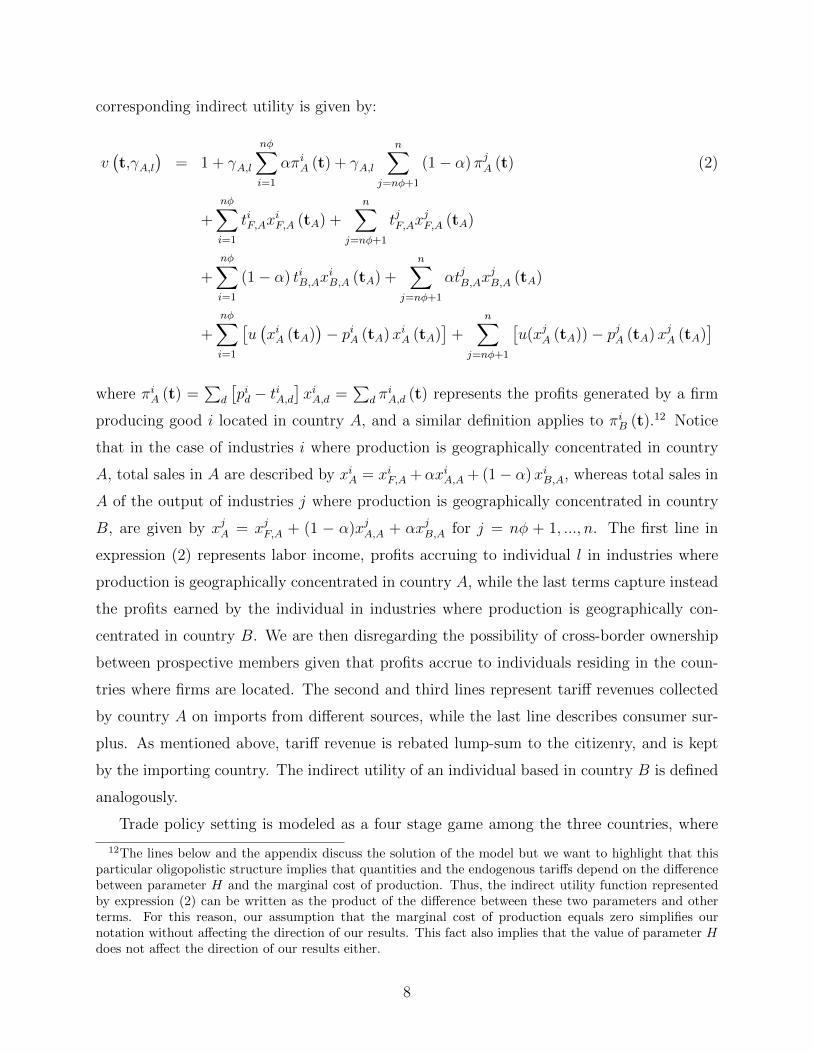
corresponding indirect utility is given by:
v(t,γA,l
)= 1 + γA,l
nφ∑i=1
απiA (t) + γA,l
n∑j=nφ+1
(1− α) πjA (t) (2)
+
nφ∑i=1
tiF,AxiF,A (tA) +
n∑j=nφ+1
tjF,AxjF,A (tA)
+
nφ∑i=1
(1− α) tiB,AxiB,A (tA) +
n∑j=nφ+1
αtjB,AxjB,A (tA)
+
nφ∑i=1
[u(xiA (tA)
)− piA (tA)xiA (tA)
]+
n∑j=nφ+1
[u(xjA (tA))− pjA (tA)xjA (tA)
]where πiA (t) =
∑d
[pid − tiA,d
]xiA,d =
∑d π
iA,d (t) represents the profits generated by a firm
producing good i located in country A, and a similar definition applies to πiB (t).12 Notice
that in the case of industries i where production is geographically concentrated in country
A, total sales in A are described by xiA = xiF,A +αxiA,A + (1− α)xiB,A, whereas total sales in
A of the output of industries j where production is geographically concentrated in country
B, are given by xjA = xjF,A + (1 − α)xjA,A + αxjB,A for j = nφ + 1, ..., n. The first line in
expression (2) represents labor income, profits accruing to individual l in industries where
production is geographically concentrated in country A, while the last terms capture instead
the profits earned by the individual in industries where production is geographically con-
centrated in country B. We are then disregarding the possibility of cross-border ownership
between prospective members given that profits accrue to individuals residing in the coun-
tries where firms are located. The second and third lines represent tariff revenues collected
by country A on imports from different sources, while the last line describes consumer sur-
plus. As mentioned above, tariff revenue is rebated lump-sum to the citizenry, and is kept
by the importing country. The indirect utility of an individual based in country B is defined
analogously.
Trade policy setting is modeled as a four stage game among the three countries, where
12The lines below and the appendix discuss the solution of the model but we want to highlight that thisparticular oligopolistic structure implies that quantities and the endogenous tariffs depend on the differencebetween parameter H and the marginal cost of production. Thus, the indirect utility function representedby expression (2) can be written as the product of the difference between these two parameters and otherterms. For this reason, our assumption that the marginal cost of production equals zero simplifies ournotation without affecting the direction of our results. This fact also implies that the value of parameter Hdoes not affect the direction of our results either.
8
different trade policy regimes can be chosen by countries A and B. In the first stage, each
prospective member holds a sequence of votes to choose between a non–discriminatory “most-
favored-nation” trade policy, a free trade area or a customs union. In the second stage, the
population of each country elects a representative who will, in the third stage, decide the
countries’ tariff policy. If no preferential agreement is in place, each country’s representative
chooses the non–discriminatory tariffs to be applied on all trade. If a preferential agreement
is in place, then the representatives of countries A and B decide tariffs only on country F .
Importantly, the formation of a free trade area does not require policy cooperation between
elected representatives when deciding tariffs on F . By contrast, the formation of a customs
union requires policy coordination when it comes to deciding on the common external tariff
vis-a-vis country F . In stage four, firms compete in quantities, taking as given the trade
policy that has been set during the third stage. We solve the model backwards, starting from
stage four which we turn to now, before analyzing the policy setting stages of our model in
the following section.
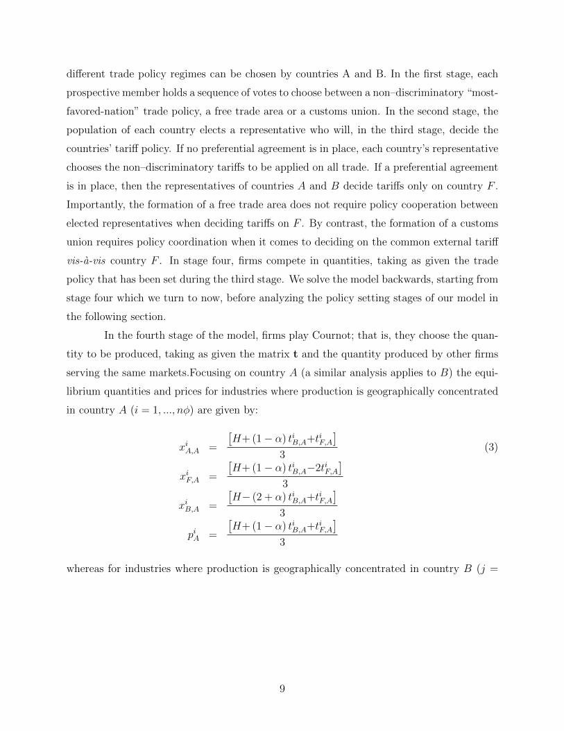
In the fourth stage of the model, firms play Cournot; that is, they choose the quan-
tity to be produced, taking as given the matrix t and the quantity produced by other firms
serving the same markets.Focusing on country A (a similar analysis applies to B) the equi-
librium quantities and prices for industries where production is geographically concentrated
in country A (i = 1, ..., nφ) are given by:
xiA,A =
[H+ (1− α) tiB,A+tiF,A
]3
(3)
xiF,A =
[H+ (1− α) tiB,A−2tiF,A
]3
xiB,A =
[H− (2 + α) tiB,A+tiF,A
]3
piA =
[H+ (1− α) tiB,A+tiF,A
]3
whereas for industries where production is geographically concentrated in country B (j =
9
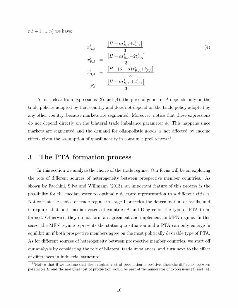
nφ+ 1, ..., n) we have:
xjA,A =
[H + αtjB,A+tjF,A
]3
(4)
xjF,A =
[H + αtjB,A−2tjF,A
]3
xjB,A =
[H− (3− α) tjB,A+tjF,A
]3
pjA =
[H + αtjB,A + tjF,A
]3
As it is clear from expressions (3) and (4), the price of goods in A depends only on the
trade policies adopted by that country and does not depend on the trade policy adopted by
any other country, because markets are segmented. Moreover, notice that these expressions
do not depend directly on the bilateral trade imbalance parameter φ. This happens since
markets are segmented and the demand for oligopolistic goods is not affected by income
effects given the assumption of quasilinearity in consumer preferences.13
3 The PTA formation process
In this section we analyze the choice of the trade regime. Our focus will be on exploring
the role of different sources of heterogeneity between prospective member countries. As
shown by Facchini, Silva and Willmann (2013), an important feature of this process is the
possibility for the median voter to optimally delegate representation to a different citizen.
Notice that the choice of trade regime in stage 1 precedes the determination of tariffs, and
it requires that both median voters of countries A and B agree on the type of PTA to be
formed. Otherwise, they do not form an agreement and implement an MFN regime. In this
sense, the MFN regime represents the status quo situation and a PTA can only emerge in
equilibrium if both prospective members agree on the most politically desirable type of PTA.
As for different sources of heterogeneity between prospective member countries, we start off
our analysis by considering the role of bilateral trade imbalances, and turn next to the effect
of differences in industrial structure.
13Notice that if we assume that the marginal cost of production is positive, then the difference betweenparameter H and the marginal cost of production would be part of the numerator of expressions (3) and (4).
10
3.1 Trade Imbalances
As pointed out already by Grossman and Helpman (1995), bilateral trade imbalances
between prospective member countries are likely to play an important role in the decision
to join a preferential trading agreement. To model their role and to keep the analysis
tractable, we focus on a situation where perfect geographic specialization prevails (α = 1).
In this case, goods in which production is geographically concentrated in country A (B)
are exported by country A (B) and only imported (not produced) by the other prospective
member. Remember that in our framework, φ = 0.5 captures the situation in which A and
B have the same number of exporting industries, and, as a result, trade is balanced between
them. If φ > 0.5, A starts running a bilateral trade surplus vis-a-vis B, that is increasing in
φ.
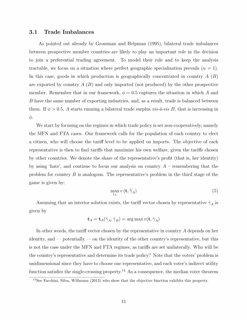
We start by focusing on the regimes in which trade policy is set non-cooperatively, namely
the MFN and FTA cases. Our framework calls for the population of each country to elect
a citizen, who will choose the tariff level to be applied on imports. The objective of each
representative is then to find tariffs that maximize his own welfare, given the tariffs chosen
by other countries. We denote the share of the representative’s profit (that is, her identity)
by using ‘hats’, and continue to focus our analysis on country A – remembering that the
problem for country B is analogous. The representative’s problem in the third stage of the
game is given by:
maxtA
v (t, γA) (5)
Assuming that an interior solution exists, the tariff vector chosen by representative γA is
given by
tA = tA(γA, γB) = arg max v(t, γA)
In other words, the tariff vector chosen by the representative in country A depends on her
identity, and — potentially — on the identity of the other country’s representative, but this
is not the case under the MFN and FTA regimes, as tariffs are set unilaterally. Who will be
the country’s representative and determine its trade policy? Note that the voters’ problem is
unidimensional since they have to choose one representative, and each voter’s indirect utility
function satisfies the single-crossing property.14 As a consequence, the median voter theorem
14See Facchini, Silva, Willmann (2013) who show that the objective function exhibits this property.
11
can be applied and the choice of the representative is the solution to the following problem:
maxγA
v (t (γA, γB) , γmA ) (6)
Solving stages 2 and 3 of the game yields the following result:
Lemma 1 Independently of the extent of trade imbalances, if tariffs are set non-cooperatively
then strategic delegation does not arise in equilibrium, i.e. γc = γmc , where c = A,B. Fur-
thermore, if an FTA is formed, tariffs applied to non-member countries are (weakly) lower
than under an MFN arrangement.
Proof. See Appendix.
The intuition for Lemma 1 is as follows. In the model, the markets for goods i and j are
segmented, and as a result the equilibrium prices in country A and B bare no relationship
with each other. Moreover, in this non–cooperative setting, the tariffs applied by country A
can differ from those applied in country B. The median voter is better off by representing
her own interests rather than delegating to someone else, as she does not have any influence
on the partner country’s decisions. The tariff complementarity result follows the same logic
as in Saggi (2006) and Ornelas (2007). In particular the decline in the tariff applied to the
non–produced goods is the result of the successful effort of the median voter to attenuate
the degree of trade diversion generated by the preferential access granted to the partner
country.15
The main difference between an FTA and a CU is that in the latter member countries co-
operate in setting a common trade policy. Following the literature, the trade policy adopted
in a CU maximizes the joint surplus of the two countries’ representatives, i.e. it solves:
maxtv (t, γA) + v (t, γB) (7)
where γA and γB are the elected representatives in the two countries and now tariffs applied
on trade with country F are equal (ti = tiF,A = tiF,B) across countries (but not necessarily
across sectors). The resulting tariff vector chosen is given by
tCU = tCU(γA, γB)
15Note that this effect is absent from the model by Grossman and Helpman (1995), since in that frameworkby assumption external tariffs do not change following the establishment of a free trade area.
12
As before, in the second stage of the model, in country A the representatives will be chosen
by the median voter as the solution to the following problem
maxγA
v(tCU (γA, γB) , γmA
)(8)
We are now ready to state our second result:
Lemma 2 Independently of the extent of trade imbalances, if trade policy is set cooperatively
then strategic delegation occurs, and the elected representative is an individual with an own-
ership share that is twice as high as that of the median voter. Moreover, if a CU is formed,
the common external tariff is higher than the tariff applied by each member of the FTA.
Proof. See Appendix.
To understand the intuition for this result, note that markets are segmented in our model
and external tariffs are not directly affected by trade imbalances (i.e. by φ). In the case of
the CU, both countries A and B benefit from the implementation of a tariff on the imports
of good i = 1, ...nφ, because the tariff lowers the exporting price of the firm based in the rest
of the world. At the same time, country A gains more than country B from the protection
applied to that sector, because it also benefits from profit shifting, whereas the costs of the
tariff are equally shared between the two countries. Cooperative tariff setting forces the
representatives to internalize the negative externality on country B from a tariff imposed on
imports of good i. Anticipating this outcome in the third stage, the median voter is better
off delegating power to a representative who is more protectionist than herself, who will then
negotiate a trade policy that the median voter prefers over the compromise she herself could
obtain.
We now proceed to study the first stage, where the trade policy regime is chosen. In
order to understand which regime is preferred by the median, it is helpful to first compare
the welfare implications of each regime. To measure welfare, we weigh equally the utility
of all individuals and focus on the average voter’s indirect utility function, v(t, γ) as our
welfare measure.
The analysis of stages 2 and 3 has shown that equilibrium tariffs as well as the degree
of strategic delegation are not influenced by the number of exporting and importing sectors
in each member country. However, the pervasiveness of trade imbalances will affect welfare
13
in each prospective member country. In particular, we know from the literature that, in our
oligopolistic trade framework, countries tend to benefit from preferential trade when they
receive preferential access, whereas they tend to lose from it when they grant preferential
access.
Under balanced bilateral trade between countries A and B, it is straightforward to show
that the overall welfare effect of a PTA is positive when we take into account the increase
in profits generated by receiving preferential access. Considering the general case, in which
partner countries exchange different degrees of market access, this result does not necessarily
hold anymore. In particular, under our assumption that φ > 0.5, country A has more
exporting sectors than country B, and, as a result, it will run a trade surplus vis-a-vis B.
In other words, A will receive greater preferential access from B than it grants in return to
the partner country, and this will have an important impact on the welfare effects of a PTA
for the two countries.
A second key force shaping the welfare impact of a PTA in each prospective member
country is represented by the shape of the income distribution, which in turn will affect
the extent of strategic delegation under the CU regime. As shown in Lemmata 1 and 2,
voters strategically delegate power to more protectionist representatives under a CU regime,
while the same is not true in the MFN and FTA cases. If inequality is very low, i.e. λm is
close to one, strategic delegation under a CU leads to very high common external tariffs, at
least from the point of view of the average voter. This might render the FTA arrangement
welfare-dominating relative to a CU.
To characterize welfare in each country we use the equilibrium tariffs under the various
regimes,16 along with equilibrium quantities and prices represented by (3) and (4), to assess
the value of the average voter’s indirect utility function under the different trade policy
regimes. Figure 1 illustrates the resulting welfare ranking for country A (top panel) and B
(bottom panel), as we vary trade imbalances (φ) and income inequality (γm).17 In particular,
as φ > 0.5 increases, country A has a greater trade surplus with B. As we move downwards
16See in particular equations (16), (17), and (22) in the appendix.17See Appendix for details on how these figures have been constructed. Notice that the cutoff values for
parameters φ and γm in Figure 1 are not affected by the other parameters of the model (H and n). Thishappens since the product between parameters H and n multiply all other terms of the expression describingthe change in the average voter’s indirect utility function. The same applies to other figures discussed below.Notice that the mathematica files used to construct Figure 1, as well as used in constructing the other figuresdescribed below, are available upon request.
14
on the vertical axis, i.e. towards a more balanced distribution of market access, we can
see that the FTA and MFN regimes may welfare-dominate a CU if the degree of income
inequality is sufficiently low (i.e. γm is high). If we instead move upwards on the vertical
axis, the welfare ranking of the various trade regimes diverges between prospective member
countries. In particular, as market access becomes more unequal (φ moves away from 0.5),
the parameter space under which an FTA raises welfare relative to a CU becomes smaller
(larger) for the partner country with a bilateral trade surplus (deficit). If inequality in market
access exceeds a threshold, a CU welfare–dominates (is dominated by) an FTA under any
distribution of income from the point of view of the partner country with a bilateral trade
surplus (deficit). The intuition for this result can be explained as follows. As we have already
discussed, the common external tariffs in the CU are larger than those adopted in the FTA.
As a result, profits tend to be greater in the CU than in the FTA. As the exchange of
preferential access becomes more unequal (i.e. φ 6= 0.5), the profits generated by preferential
access become more important for the country with a bilateral trade surplus, and less so for
that with a deficit. It follows that the size of the parameter space under which CUs raise
welfare relative to FTAs increases for the former, while it decreases for the latter.
[INSERT FIGURE 1 HERE]
A comparison between the MFN and different PTA regimes yields similar results. If the
exchange of market access is balanced (φ close to 0.5), the FTA leads to higher welfare than
the MFN regime for both A and B, regardless of income distribution. As the exchange of
market access becomes more unequal, this result continues to hold for the country with a
bilateral trade surplus regardless of income distribution. The opposite is true for the country
with a bilateral trade deficit regardless of income distribution. A similar analysis also applies
to the case of a CU. Under a balanced exchange of market access, a CU is welfare-enhancing
relative to the MFN regime unless income inequality is sufficiently low. As inequality in the
exchange of market access increases, the policy space under which a CU raises welfare relative
to the MFN regime becomes greater (smaller) in the country with a bilateral trade surplus
(deficit). Thus, the general message from the welfare comparison of the different regimes is
that the benefits of entering a preferential trade agreement tend to increase (decrease) for
the prospective member country with a trade surplus (deficit), the more unequal preferential
market access is.
15
We can now turn to the solution of the first stage of the game, in which the choice of trade
policy regime is determined by the median voter. We assume that citizens choose among
the different trade policy regimes using a sequence of referenda. In the first referendum, the
citizenry chooses between the MFN (status quo) and the FTA regimes, while, in the second
referendum, it decides between the trade regime that wins the first referendum and a CU.18
For a PTA to be politically viable, the median voter’s welfare must increase as the economy
moves from a MFN regime to the PTA. To understand the role of the various forces at play
in determining whether this is the case, it is useful to decompose the change in the median
voter’s indirect utility as follows:
∆v(tMFN , tPTA, γmA
)= ∆v
(tMFN , tPTA, γA
)︸ ︷︷ ︸Social welfare
− (1− γmA )︸ ︷︷ ︸Inequality
(∆π1
A
(tMFN , tPTA
))︸ ︷︷ ︸Pr ofits
(9)
where ‘∆’ represents the change in variables from the MFN regime to a PTA. Since the
profits of member countries’ firms increase if they are granted preferential access under a
PTA, equation (9) highlights that politically viable PTAs must be welfare enhancing. It also
shows how profits are less important in determining the political desirability of the PTA,
compared to their appeal from the point of view of national welfare, as the median voter
receives a lower share of profits than the average voter.
Figure 2 illustrates the political viability of the three trade regimes for country A (top
panel) and B (bottom panel).19 As can be seen from the diagrams’ lower edges, an FTA will
emerge as a political equilibrium, if income inequality is sufficiently low (γm is sufficiently high)
and if there is a balanced exchange of preferential market access across prospective member
countries (φ close to 0.5). This is because, as shown in Figure 1, if the exchange of bilateral
trade access is balanced then an FTA is welfare-enhancing relative to both the MFN regime,
regardless of income distribution, as well as the CU if inequality is sufficiently low, and an
FTA tends to be politically more appealing than a CU given that profits are less important
from the political than in terms of national welfare.
[INSERT FIGURE 2 HERE]
18Alternatively, we could start by considering the decision between the MFN arrangement and a CU andthen, in the second stage, pit against each other the winner and the FTA. The two sequences deliver thesame outcome.
19See Appendix for details of the calculations.
16
The outcome changes if the exchange of preferential market access is unbalanced (φ above
.5). In particular, as φ increases, so does the parameter space under which a CU is country
A’s politically preferred choice. At the same time, the parameter space in which any PTA
is politically viable in country B decreases. As φ increases, B grants, by entering into a
PTA with A, an increasing amount of preferential access to A, while it receives less and
less preferential access in return. Note also that the interaction between bilateral trade
imbalances and income inequality does not play a clear role in determining the political
viability of an FTA compared to a CU regime.
Summing up, the presence of bilateral trade imbalances suggests that the political via-
bility of a PTA depends primarily on whether it is supported in the prospective member
country with a trade deficit. In fact, as trade imbalances become more severe, the policy
space where a PTA is politically viable decreases since the country facing a trade deficit is
less keen on granting more preferential access than it receives.
3.2 Geographic Specialization
We now turn to study the effect of varying the degree of geographic specialization.
Recall that a measure α ∈ [0.5, 1] of firms in industries that are concentrated in country
A is located in that country (and similarly for firms in industries that are concentrated in
country B). It follows that each prospective member country is a net exporter to the other
prospective member of the goods produced in these respective industries. Each economy
continues to be characterized by the presence of n oligopolistic industries but, in order to
keep the analysis tractable, we now restrict the analysis to balanced trade between the two
countries, i.e. we assume in this subsection that φ = 0.5.
As in the previous section, we solve the game by first focusing on the non-cooperative
trade regimes (FTA and MFN) and then turn to analyze the setting of a common external
tariff under a customs union. We can establish the following:
Lemma 3 In the presence of imperfect geographic specialization, if trade policies are set
non–cooperatively, strategic delegation does not arise in equilibrium. Furthermore, if an
FTA is formed, tariffs applied to non–member countries are (weakly) lower than under an
MFN arrangement.
Proof. See Appendix.
17
We can now consider the case of a CU, where the external tariff is chosen so as to
maximize the joint welfare (the sum of the indirect utilities) of the two countries’ represen-
tatives. We can establish the following:
Lemma 4 In the presence of imperfect geographic specialization, if trade policy is set coop-
eratively, strategic delegation occurs, and the elected representative is an individual with an
ownership share in the import competing industries that is higher than that of the median
voter. Furthermore, strategic delegation increases with the degree of geographic specialization.
Proof. See Appendix.
We turn now to study the political viability of the different regimes. As in section 3.1,
a useful intermediate step involves the analysis of the social welfare levels under the three
regimes. Two features of our model play an important role in shaping the welfare outcomes.
First, as the median is poorer than the average voter, if income inequality increases so does
the gap in the trade policy preferences of the median and average voters. Second, the median
voter may decide to delegate power instead of representing himself. In particular, strategic
delegation occurs in the case of a CU, and it increases with geographic specialization, whereas
it is not present in the MFN and FTA regimes. This results in a positive relationship between
geographic specialization and common external tariffs for a CU.
Figure 3 illustrates the welfare ranking of the different trade policy regimes for each
prospective member country. As we can see, increasing the degree of geographic special-
ization (α increases), implies that the FTA and MFN welfare dominate the CU if income
inequality is sufficiently low. The intuition for this result is that the higher geographical
specialization, the more pronounced becomes strategic delegation under the CU regime (see
equation 26 in the Appendix). If income inequality is low (γm is high), this results in very
protectionist representatives being chosen under the CU regime. If countries become more
similar, by contrast, the policy space in which a CU welfare dominates both the FTA and
MFN regimes clearly expands, as strategic delegation under the CU is mitigated, and the
benefits from tariff coordination dominate.
[INSERT FIGURE 3 HERE]
Turning now to the choice of the median voter, his ranking of the possible outcomes is
illustrated in Figure 4. As geographic specialization increases, we know from Figure 3 that
18
a CU may be welfare-dominated by both the MFN and FTA regimes if the degree of income
inequality is sufficiently low. In this case, the CU will never be chosen by the median voter
(see the discussion following equation 9). As countries become more similar, once again
the political prospects of a CU increase, as long as the degree of income inequality is not
too high (see the bottom right section of Figure 4). Note also that the interaction between
geographic specialization and inequality may play an important role in the choice between
forming an FTA or a CU. For low to medium ranges of geographic specialization,20 an FTA
is politically more palatable than a CU if income inequality is sufficiently low. Otherwise, a
CU will be chosen.21
[INSERT FIGURE 4 HERE]
4 Main Predictions and Dataset
Our theoretical model allows us to formulate a series of hypotheses that can be empiri-
cally assessed. Importantly, it enables us to distinguish between factors that directly affect
the decision to form a PTA, and those that instead impact the type of PTA that will be
chosen. In this section we start by discussing our hypotheses, and will then present the data
employed in the analysis.
4.1 Main Predictions
Our first prediction focuses on the role played by income inequality and trade imbalances in
determining the political viability of PTAs. Building on the analysis carried out in Section
3, and focusing on Figure 2 to understand the effects of trade imbalances and on Figure 4
for the role of geographic specialization, our model indicates that no PTA will emerge in
equilibrium if income inequality is too high. Turning to the role of trade imbalances, our
20I.e. for (0.84 < α < 0.9).21For a more detailed discussion of this case see Facchini, Silva, Willmann (2013). As already pointed
out in footnote 11, our framework can be extended to consider cross-border ownership between prospectivemember countries. The analysis of the effects of cross-border ownership is similar to that of geographicspecialization and both lead to broadly similar conclusions. Assuming that bilateral trade is balanced, aswell as the presence of perfect geographic specialization, we find that the more unbalanced (balanced) iscross-border ownership, the more likely will be an FTA (a CU) to emerge in equilibrium if income inequalityis not too high.
19
discussion in Section 3.1 highlights how the viability of a PTA crucially depends on the
support it gains in the prospective member country with a trade deficit. In particular, the
greater the trade imbalances, the less likely will be a PTA to emerge in equilibrium, as a
larger amount of preferential access is granted by the country with a trade deficit in exchange
for a smaller amount received by the partner country. We can summarize these results in
the following:
Hypothesis 1 (i) If inequality is sufficiently high then a PTA will not emerge in equilibrium;
(ii) If trade imbalances are sufficiently high then a PTA will not emerge in equilibrium.
While income inequality and the pervasiveness of trade imbalances are behind the decision
to establish a PTA, our model suggests that these factors do not affect the popularity of FTAs
relative to CUs. The equilibrium choice of one PTA regime over the other depends instead
on the extent of geographic specialization. This factor plays an important role because
it determines the extent of strategic delegation in a CU, which may lead to the common
external tariffs being inefficiently high. In fact, if the degree of geographic specialization
is very high (α close to 1), equation (26) indicates that the elected representative will be
significantly more protectionist than the median voter in the CU regime, whereas no strategic
delegation occurs in an FTA. This might make the FTA the equilibrium choice as shown
in the upper-right region in Figure 4. If geographic specialization is instead low (α close to
0.5), a CU will emerge. These results are summarized in the following:
Hypothesis 2 If a PTA is formed, and the degree of geographic specialization is sufficiently
high, then an FTA emerges in equilibrium. Otherwise, a CU will be formed.
Moreover, as argued in section 3.2, for intermediate levels of geographic specialization,
the formation of an FTA becomes politically viable if the degree of income inequality is
sufficiently low. Otherwise, a CU may be formed. We will test this ancillary prediction,
along side with other robustness tests, in the empirical section. We are now ready to discuss
the dataset used to test hypothesis (1) and (2) followed by a description of the econometric
strategy.
4.2 Dataset
To assess the implications of our model, we have collected a large dyadic panel dataset
with country-pair information that covers 136 countries over the period 1960-2005, at five–
20
year intervals. We follow Egger and Larch (2008) and Baier, Bergstrand and Feng (2014) in
focusing on data at this frequency. The reason behind our choice is that preferential trading
agreements are typically accompanied by long implementation periods, and data at five year
intervals are more likely to account for this than higher frequency data. Descriptive statistics
for the variables used in this study can be found in Table 1. The four columns reflect the
different dimensions of the dataset that we want to explore. In particular, column 1 provides
the average and standard deviation for each variable in the entire sample, whereas column 2
provides the same information focusing on country-pairs belonging to the same PTA. Column
3 restricts the attention to country-pairs belonging to the same FTA, and column 4 focuses
on country-pairs in the same CU.
[ Table 1 here ]
To capture the presence of a preferential trading agreement between a country pair, we
have used information from Mattevi (2005), who has classified existing agreements based on
de facto characteristics, distinguishing among FTAs, CUs and partial agreements. Partial
agreements typically involve selective sectoral trade liberalization, whereas under FTAs as
well as under CUs trade among members is substantially duty free. In the case of CUs,
member countries must have additionally agreed upon and implemented a common external
tariff for the vast majority of products.22 Given that our theoretical analysis explains the
formation of FTAs and CUs, our empirical work will focus on these two types of agreements
exclusively.
In particular, we construct two variables. The first, PTAabt, takes a value of one if at
time t a preferential trade agreement is in place between country a and b. The second,
FTAabt, characterizes instead different types of agreements, and takes a value of one if at
time t a Free Trade Area is in place between country a and b, and zero if instead a CU is in
force. Columns 1 and 2 of Table 1 indicate that – 1197, or 4 percent of the total represent
full-fledged preferential trade agreements taking the form of CUs or FTAs. This is in line
with the dataset used in Baier, Bergstrand and Feng (2014) that report a total number of
22This requirement is important as not all negotiated agreements have been implemented. For exampleMERCOSUR members have agreed and implemented a common external tariff for more than 80 percent ofthe products they trade, and as a result MERCOSUR is described as a CU in our dataset. On the otherhand, members of the Andean Community have agreed to implement a common external tariff but havefailed to follow through with that decision before 2000. As such, the Andean community is not described asa CU in our dataset.
21
country pairs belonging to the same FTA or CU equivalent to about 5 percent of their total
sample. Note also that according to Table 1, a full 55 percent of these observations are
represented by country pairs belonging to an FTA, while the rest belongs to a CU.23 As
several recent efforts have been carried out to collect information on existing preferential
trading agreements, we have assessed the robustness of our results using alternative datasets
made available by Egger and Larch (2008) and Baier, Bergstrand and Feng (2014).
Among the determinants of the formation of a PTA emphasized in the theoretical model,
our measure of inequality INEQabt is given by the net Gini coefficient24 taken from Solt
(2009) Standardized World Income Inequality Database.25 In particular, we use the highest
net Gini coefficient within a country-pair as our model suggests that - ceteris paribus - it will
be the country with the highest inequality in a country-pair to find a PTA less politically
sustainable. A comparison between columns 1 and 2 of Table 1 suggests that the average
inequality of the most unequal country in a pair for the entire sample (41.80) is higher than
the average for the most unequal country in a pair that belong to the same CU or FTA
(36.74). This is broadly consistent with Hypothesis 1 from our theoretical model, suggesting
that for a PTA to be established, inequality within member countries should be relatively
low. Turning to trade imbalances, our measure IMBabt is built using information on bilateral
trade flows from the IMF’s direction of trade database.26 In particular, it is defined as the
difference between bilateral exports in both directions between the two countries of a given
country-pair, divided by the summation of the two bilateral exports for the same pair of
countries.27 This measure can range between zero, when trade is balanced, and unity (or
100 percent), when trade is unidirectional. Our dataset highlights that trade between country
pairs is typically highly unbalanced, with a gap between bilateral exports averaging 64% of
total bilateral trade. However, the same figure is substantially lower for countries belonging
23This is in line with Figure 1 in Freund and Ornelas (2010).24The net Gini coefficient takes into account possible income redistribution promoted by national govern-
ments through the tax system. Solt (2009) finds that the degree of inequality on a net-basis is significantlylower than on a gross-basis in particular in developed countries.
25Solt standardized previous data on inequality constructed by the United Nations, making informationavailable for 153 countries starting from 1960.
26This is the same source used by Subramanian and Wei (2007), among others.27More precisely IMBabt is defined as
IMBabt =|Expabt − Expbat||Expabt + Expabt|
(10)
where Expabt is the value of exports from country a to country b at time t etc.
22
to the same FTA or CU, reaching only 34% of total bilateral trade, or, equivalently, 53%
of the average trade imbalance recorded for the entire sample. Again, this is in line with
Hypothesis 1, suggesting that the PTA’s are more likely to emerge when trade imbalances
between prospective members countries are low. Interestingly, our data indicate that trade
imbalances are higher among FTA members than among members of a CU.
As for the factors that according to our model should determine the type of PTA to
be established, we measure the degree of geographic specialization using information on the
share of total value added generated from agricultural, manufacturing and service activities
in the gross domestic products for each country. More specifically, consider a pair formed by
country a and b and denote the service, industry and agriculture share of GDP in country i
by SERi, INDi, and AGRi respectively, where i ∈ {a, b}. Then, the degree of geographical
specialization between countries a and b is defined as:
GEOabt = |SERat − SERbt|+ |INDat − INDbt|+ |AGRat − AGRbt| .
This index can take values between [0, 2], with a greater value indicating greater specializa-
tion.28 Our choice of indicator is inspired by the index of regional industry specialization
described by Krugman (1991), and has the advantage of requiring information that is avail-
able from the World Bank’s World Development Indicators dataset over a long time period
and for the large number of countries included in our analysis. Column 1 of Table 1 sug-
gests that on average the country–pairs involved in our sample differ in their reliance on
a particular economic activity by 42 percentage points. Country pairs involved in a PTA
are more similar (the corresponding figure is 23 percentage points). More importantly, a
comparison between columns 3 and 4 reveals that the extent of geographic specialization
for members of an FTA is 29 percentage points, which is far greater than the degree of
geographic specialization of CU members which is equal to 15 percentage points. This is in
line with Hypothesis 2, which suggests that the extent of geographic specialization should
be greater among members of an FTA than among members of a CU.
In our analysis we will also control for a series of additional drivers that have been shown
in the literature (see Baier and Bergstrand 2004, Egger and Larch 2008) to play a signifi-
cant role in the formation of a PTA. More specifically, we include information on the total
28If the production structure in the two countries is identical, GEOabt = 0; on the other hand, if the twocountries are completely specialized in a different sector of the economy, GEOabt = 2.
23
economic size of each country-pair (GDPSUM abt), the inverse of the distance between two
trade partners (NATURALab), an indicator for whether countries in a pair are located on the
same continent (DCONTab), the weighted average of the distance between the two countries
and third-country trade partners (REMOTEabt), the similarity in the economic size be-
tween two trade partners (GDPSIMabt), the relative factor endowment asymmetry between
two trade partners (DKLabt), the squared-value of the bilateral relative factor asymmetry
(SDKLabt), and the average relative asymmetry in factor endowments between each country
in a country-pair and other trade partners (DROWKLabt). The recent literature has also
pointed out that the formation of a PTA between countries in a pair may either encourage the
formation of other PTAs or may lead to the enlargement of existing agreements. To account
for this possibility, we additionally control for the index of interdependence (INTERDabt)
among PTAs proposed by Egger and Larch (2008) and further developed also by Baldwin
and Jaimovichi (2012).29 We represent this group of additional drivers of the formation of
PTAs by the matrix X and we construct these variables using Subramanian and Wei’s (2007)
dataset. More details on the exact definitions of each of these variables can be found in Table
A1 of the appendix.
5 Empirical Analysis
This section has two main objectives. First, we will lay out the econometric strategy im-
plemented to assess the predictions of our theoretical analysis. Second, we will present our
results, and investigate their robustness.
5.1 Specification
Following the spirit of our theoretical framework and the existing empirical literature,
we can model the formation of a preferential trade agreement as a two-step process, where
countries first decide whether to form a PTA (Hypothesis 1) and then agree on its type (Hy-
pothesis 2), i.e. on whether the PTA will be an FTA or a CU. Thus, we have a combination
of self-selection into a PTA in the first stage, and a binary decision about its type (CU or
FTA) in the second stage, a setting which can be empirically examined using a probit model
29We thank the authors for sharing their measure of interdependence with us. See Table A1 for the exactdefinition.
24
in the presence of selection developed by Van de Ven and Van Pragg (1981).
Our strategy represents a natural extension of the econometric approaches followed in
the literature. For instance, Baier and Bergstrand (2004) specify a probit model on a cross-
sectional dataset to investigate the determinants of the formation of preferential trade agree-
ments. Egger and Larch (2008) specify a similar model, but on a panel dataset, to investigate
the role played by interdependence in the formation of PTAs. A similar methodology has
also been implemented by Bergstrand and Egger (2013) to analyze the determinants of bi-
lateral investment treaties. As it is well known, in the context of a binary response model,
using (country-pair) fixed effects to account for unobservables may give rise to the incidental
parameters problem. To address this concern, Chamberlain (1980) suggests to use instead
the average of time-variant explanatory variables to obtain consistent estimates of the pa-
rameters of interest. Following Egger and Larch (2008) and Baldwin and Jaimovich (2012)
we implement this strategy in all our specifications.30
The first stage decision is described by the following specification:
PTAabt = α0 + α1INEQab,t−5 + α2IMBab,t−5 + βXab,t−5 + εabt (11)
where PTAabt is a binary variable that takes a value of 1 if a country-pair ab is part of the
same CU or FTA in year t, and zero otherwise, and IMBabt and INEQabt are respectively our
measures of trade imbalances and income inequality. Matrix X contains a set of additional
drivers of the formation of a PTA, which have been identified in the existing literature and
which we include as controls.
As the establishment of a preferential agreement between a pair of countries is likely to
affect their overall economic structure, using contemporaneous characteristics of the country
pair might lead to parameter estimates that are biased due to reverse causality. To mitigate
this concern, we follow Egger and Larch (2008) and Bergstrand and Egger (2013) among
others,31 and lag all right hand side variables. In most specifications we also include year
fixed effects to control for common time specific shocks. Our theoretical model provides clear
predictions on the expected sign of the coefficients α1 and α2. In particular, Hypothesis (1)
30In their study of third countries’ impacts on the formation of PTAs, Chen and Joshi (2010) use insteada linear probability model to allow for a rich set of country fixed effects.
31In a robustness check, we also report results for a specification in which we lag our right hand sidevariables by 10 years in order to control for the fact that some PTAs may have a longer phase-in process,obtaining similar results.
25
suggests that the greater is the trade imbalance (IMBabt) within a country-pair, and the
greater is the degree of income inequality (INEQabt), the less likely it is for a PTA to emerge
in equilibrium. As a result, we expect α1 < 0 and α2 < 0.
The second stage decision is then captured by the following binary model:
FTAabt = θ0 + θ1GEOab,t−5 + vabt (12)
where FTAabt is a binary variable that equals 1 if an FTA is in place for country-pair ab in
year t, and zero if instead a CU is in force. GEOabt is a measure of the degree of geographic
specialization for a country-pair. Our theoretical model provides a clear prediction on the
expected sign of θ1. Hypothesis (2) indicates that, if a PTA is formed, the higher the degree
of geographic specialization (GEOabt), the more likely is an FTA to emerge as a political
equilibrium. As a result, we expect θ1 > 0. In line with the discussion in Section 3.2, we
also control for the interaction between income inequality and geographic specialization as
a robustness test. Also in this case, the explanatory variables are lagged to mitigate reverse
causality concerns. The error terms εabt and vabt are assumed to be bivariate, zero mean
normally distributed with correlation coefficient ρ.
5.2 Econometric Results
Table 2 contains our main results, which are presented in two panels. The top panel
reports the findings from the estimation of the selection equation (equation 11) modeling the
determinants of the PTA formation decision, whereas the lower part contains the estimates of
the latent equation (equation 12), describing the choice of PTA type. Column (1) reports the
results of a pooled OLS regression, whereas column (2) contains our benchmark analysis,
which accounts also for year fixed effects. To help quantifying the economic magnitudes
involved, in column (3) we report the corresponding marginal effects. The latter capture the
change in the probability of forming a PTA (respectively forming a Free Trade Area) due to
an infinitesimal change in each independent, continuous variable, and a discrete change in
the probability for dichotomous variables.
[Table 2 here]
The LR test reported at the bottom of the table indicates that the probit model with
26
sample selection performs better than estimating equations (11) and (12) separately. Fur-
thermore, the empirical findings shown in column 1 provide broad support for our theoretical
predictions. Focusing on the determinants of the formation of a PTA (upper panel), we find
that an increase in income inequality is negatively related to the probability that a PTA will
be established between two countries, even if the effect is not statistically significant. Simi-
larly, an increase in bilateral trade imbalances tends also to significantly reduce the likelihood
that a PTA will be put in place. These findings are in line with the predictions summarized
in Hypothesis 1. As for the control variables, our analysis confirms patterns that have al-
ready been uncovered in the existing literature (see in particular Baier and Bergstrand 2004
and Egger and Larch 2008). In particular, we find that a PTA is more likely to emerge if two
countries are geographically closer (NATURAL) to each other, if they belong to the same
continent (DCONT ), if other country-pairs are part of pre-existing PTAs (INTERD), if
they are more remote from the rest of the world (REMOTE), if their total market size
(GDPSUM) is larger, if they are more similar in terms of their economic size (GDPSIM)
and if their factor endowments (DKL) are more dissimilar. As it has also been found by
previous studies, the effect of the latter is non linear, and it is increasing, but only up to a
point (the sign of SDKL is negative), whereas the likelihood of establishing an agreement
is expected to decrease in the relative factor endowment difference between the rest of the
world and a given country-pair (DROWKL). However, the last prediction is not confirmed
by our data.
Turning to the choice of the agreement type (bottom panel of Table 2), we find that
if a PTA has been formed, an FTA is more likely to emerge if the production structure
of the countries in the pair is more heterogeneous. These results provide strong support
for the predictions of our theoretical model summarized in Hypothesis 2. Notice that the
patterns uncovered in column 1 are confirmed and reinforced when we account additionally
for time varying common shocks in column 2.32 In particular, the direct effect of inequality
in the PTA formation equation is now statistically significant at the 5% level. Moreover, the
effects we have identified are economically important, as illustrated by the marginal effects
reported in column (3). For instance, a one standard deviation increase in our measure of
inequality decreases the probability that a country-pair forms a PTA by about 1 percentage
32We have also run specification (2) using the different interdependence index proposed by Baldwin andJaimovichi (2012), and obtained similar result. These results are available from the authors upon request.
27
point – a large effect given that in our sample the probability of a country pair belonging
to a PTA is only 4 percent.3334 The same holds when we consider the determinants of the
choice between an FTA and a CU. In particular, a one standard deviation increase in our
measure of geographic specialization leads to an increase of 5.36 percentage points in the
likelihood that an FTA – rather than a CU – will emerge in equilibrium.
The results we have reviewed so far indicate that the basic predictions of our model are
supported by the data. At the same time, it is interesting to investigate how well do our
benchmark specification predicts the actual formation of PTAs and their type. The former
can be studied by using the fitted probabilities from the selection equation, and the latter
by considering the fitted probabilities from the latent equation. As we pointed out in section
4.2, the formation of a PTA is a rare event – out of 29870 country-pair observations in
our sample, only 1197 or 4 percent of the total have a PTA in place. Moreover, among
country–pairs with a PTA, 55 percent of the observations are represented by FTAs and 45
percent by CUs. Following Bergstrand and Egger (2013) we use this a priori information
about the proportion of events (PTA formation and FTA/CU formation) and non–events to
form cutoff probabilities for the percent of correctly predicted, both for “true positives” and
“true negatives”. Focusing on the selection equation, our model successfully predicts 90.8
percent of the observations involving country pairs actually belonging to a PTA. Moreover,
our benchmark specification is also able to predict 89.1 percent of the observations involving
country pairs that do not belong to a PTA. Turning to the choice between an FTA and a
CU (described by the latent equation), our model is able to correctly predict 74.6 percent
of the 665 country-pairs that belong to the same FTA, whereas it can correctly predict
88.3 percent of the 532 country-pairs that belong to the same CU. Overall, the empirical
benchmark model correctly predicts 80.7 percent of the choice between an FTA and a CU
for the country-pairs that have decided to form a PTA.
33The economic effects of the different variables used in our econometric model can be obtained by mergingthe information on descriptive statistics shown in Table 1 with the marginal effects shown in the last columnto the right of Table 2. For instance, a one-standard deviation increase of income inequality in our sampleequals to 9.91 according to column 1 of Table 1. We can then multiply this standard deviation by themarginal effect of income inequality, equal to -0.001 according to Table 2, and obtain the economic effect ofabout -0.01 (1 percentage point) discussed in this paragraph.
34Notice that a one-standard deviation increase in our measure of trade imbalance leads to a decrease of0.34 percentage points in the probability that a country-pair forms a PTA.
28
5.3 Robustness checks
In this section, we consider a number of extensions to our benchmark analysis. In Table
3 we focus on additional factors that might affect the choice between the formation of an
FTA and a CU. As we already discussed in the introduction of this paper, the literature on
the choice between different types of preferential trade agreements is sparse. One interesting
example is a recent paper by Lake and Yildiz (2016), who consider a three-country model in
the presence of geographical asymmetries. In their setting some countries are located closer
to each other than others, and hence the former face lower trade costs than those that are
further away. Their theoretical analysis indicates that there is a distance cut-off above which
an FTA is the only viable choice of PTA. This suggests that the greater the geographical
distance between the countries in a pair, the more likely it will be for an FTA rather than a
CU to emerge in equilibrium. We assess this prediction — which is complementary to ours
— in column (1), where in the bottom panel (latent equation) we control for the inverse
of the distance between trade partners. Interestingly, we find evidence corroborating this
theoretical result: for the average country-pair and year, if they enter a PTA, more closely
located countries are more likely to form a CU rather than an FTA. Importantly though,
accounting for this additional factor does not affect our main results.
[Table 3 here]
The role of alternative sources of asymmetries across potential member countries in the
formation of CUs or FTAs – like those which lead to different market sizes – has also been
considered in the literature.35 For this reason, in column (2) we additionally control for the
degree of market size asymmetry for countries in each pair. Our findings indicate that coun-
tries of more similar size are more likely to form an FTA rather than a CU, but importantly
accounting for this additional driver does not affect our main results.
In Table 4 we investigate the robustness of our main findings. Hypothesis 1 indicates
that trade imbalances between prospective member countries may prevent the formation
of a preferential trade agreement, and the results discussed above provide support to this
prediction. The specifications used in columns (1) and (2) of Table 4 assess the robustness
of our findings by using alternative measures of bilateral trade imbalances.
35See for instance Melatos and Woodland (2007) which have used a calibrated general equilibrium modelto investigate the role played by consumer preference asymmetries and export endowment asymmetries indetermining whether a CU or an FTA should emerge in equilibrium.
29
We start by exploiting Rauch (1999) classification of traded goods in three broad cate-
gories, i.e. those traded in organized exchanges, those that are “reference priced” and those
that are truly differentiated, and construct a measure of trade imbalances focusing only on
differentiated goods (see column 1).36 In column (2) we consider instead overall trade im-
balances as in our baseline specification, but use an alternative definition of the variable. In
particular, we measure trade imbalances using the absolute value of difference between the
bilateral exports for a country-pair divided by the total trade of the country running a bi-
lateral trade deficit.37 The results shown in these specifications indicate that the qualitative
conclusions of our benchmark analysis are not affected by changing our measure of trade
imbalances.38
To address reverse causality concerns, our specifications so far have employed five–year
lagged values for our explanatory variables. In column (3) we assess the robustness of
our findings to the introduction of ten –year lags to capture longer term determinants of
the preferential trading agreement formation process. Once again our results are broadly
unaffected. A large fraction of the preferential trading agreements considered in our paper
came into force towards the end of the 20th century. In column (4) we thus study whether
our model can help explaining the formation of only these most recent agreements, focusing
on the years 2000 and 2005. While the magnitude of the coefficients are affected – and
in particular the role of trade imbalances appears to be bigger, the basic patterns we had
uncovered in our benchmark specification continue to hold.
The introduction of this paper points out that the formation of FTAs is far more popular
than the formation of CUs. Still, the first and one of the most popular PTAs is the European
36The classification used in column (1) to identify differentiated goods is labeled as “liberal” in Rauch(1999). Using the alternative, “conservative” classification yields qualitatively similar results.
37In this robustness test, we define trade imbalance IMBabt as
IMBabt =|Expabt − Expbat|
|Ia × (IMPat + Expat) + (1− Ia)× (IMPbt + Expbt)|(13)
where Expabt is the value of exports from country a to country b at time t, Expat (IMPat) is the value ofcountry a’s total exports (imports) at time t, Ia is a dummy variable that equals one if country a runs abilateral trade deficit with country b (Expabt < Expbat) and etc.
38Notice that both these alternative measures of trade imbalances can be related to our model. Thebilateral imbalance between countries A and B originate in non-numeraire industries, where firms competein a Cournot fashion. It is clear that imperfect competition is more related to differentiated rather thanhomogenous goods and this justifies the alternative measure used in column (1). Likewise, the fate of thepreferential trade agreement rests with the country running a bilateral trade deficit according to our model.Thus, the model also justifies the alternative measure of trade imbalance used in column (2).
30
Union (EU), which is classified as a CU in our dataset, and has gone through five rounds
of expansion since its inception in 1957. A total of 25 member countries were part of the
EU by year 2005. In column (5) we investigate whether our main predictions are robust to
dropping the substantial number of CU country-pairs related to the formation of the EU from
our sample. The results suggest that our predictions are robust to dropping CU country-
pairs related to this important PTA.39 As we pointed out before, the number of preferential
trading agreements has rapidly increased over time. Importantly, various efforts have been
carried out to collect systematic information on the nature of the various agreements in
force, and some of the existing databases focus more on de jure criteria, whereas others put
more weight on de facto considerations. It is therefore important to assess the robustness of
our analysis to the use of alternative datasets proposed in the literature. In column (6) we
present the result of the analysis when our left hand side variables (PTA formation decision
and choice between a CU and an FTA) are constructed using the recent database constructed
by Egger and Larch (2008). In column (7) we use instead the dataset collected by Baier,
Bergstrand and Feng (2014). While some differences exist, the information contained in
the data collected by Mattevi (2005) and in these alternative sources are broadly similar.
Importantly, using these alternative measures does not affect our results: the qualitative
patterns we have uncovered in column 2 of Table 2 continue to hold, and even the magnitudes
of the effects of our main explanatory variables are comparable.
A key result of our theoretical framework is summarized by Hypothesis 2 and it posits
that the more asymmetric the production structures of two prospective member countries
(i.e., the greater the degree of geographic specialization), the more likely it is that an FTA
will emerge in equilibrium if the two countries decide to form a PTA. The results described
above provide strong support to this prediction. One ancillary prediction of our theoretical
model is that the effects of geographic specialization will be stronger, the less unequal is the
income distribution in the country pairs. We assess this prediction in column (8) of Table
4 (bottom panel) finding support for this additional implication of our model. However,
notice that the coefficient of income inequality in the latent equation (bottom panel) is not
statistically significant, indicating that income inequality does not directly affect the choice
of PTA type. This result is in line with Hypothesis 1.
39Table 1 indicates that 532 country-pairs in our sample are members of CUs. Moreover, 388 of these pairscorrespond to members of the European Union. This fact means that 74 percent of our CU country-pairsare related to the EU.
31
[Table 4 here]
Likewise, our theoretical model suggests that trade imbalances should play a key role in
shaping the decision to form a PTA. At the same time it does not provide a clear prediction
for their role in affecting the choice between a CU or an FTA. In column (9) we explicitly
address this question, by directly controlling for the extent of trade imbalances in the latent
equation. Our results indicate that trade imbalances do not affect the choice of PTA type.
Importantly, the inclusion of this control does not affect our main results. In summary, the
results described in columns (8) and (9) of Table 4 provide additional support to Hypothesis
1 since we confirm that income inequality and trade imbalances should affect directly the
decision to form a PTA, rather than the choice of its type.40
6 Conclusion
In this paper we have developed a political economy model that provides novel insights
into the process of forming a PTA, where we distinguish between those factors that affect
the decision to form a PTA, and those that matter for the choice of its type (FTA or CU).
Our analysis suggests that bilateral trade imbalances and income inequality are key variables
in the decision to form a PTA. This means that only if bilateral trade between prospective
members is sufficiently balanced, and income inequality is sufficiently low, trade partners
find a PTA to be politically viable. As for which type of agreement to choose, i.e. whether
they form an FTA or a customs union, our framework suggests that this depends on the
extent of differences in the production structure between prospective member countries.
We then proceed to assess empirically these implications of our theory, using a sample of
more than 100 countries covering the period 1960–2005. Our empirical analysis finds strong
support for the predictions of the model. In particular, the greater income inequality and
bilateral trade imbalances, the less likely is a country-pair to have a joint PTA in place.
Furthermore, we also find that the greater the asymmetries in production structure between
two countries, the more likely it is for us to see an FTA between them instead of a CU. We
40We have carried out additional robustness tests to confirm the predictions outlined in hypotheses 1 and2. In particular, we have estimated our probit with sample selection model using data from 1960 to 2000,as well as estimated it using explanatory variables measured at the same year of the dependent variables(i.e., not lagged explanatory variables). In both cases the results tend to provide support to our predictionsoutlined in hypotheses 1 and 2. These additional results are available upon request.
32
also confirm the role played by a few other factors suggested by the literature in determining
the choice between an FTA and a CU, but, importantly, these additional factors do not
affect our main empirical results.
Proposing new theoretical insights into the process of PTA formation, and checking these
predictions against the data, is highly relevant in light of the ever increasing number of PTAs
that are in force, or in the process of being formed. Given that the multilateral approach
of the GATT/WTO has slowed to a stand-still, the question of whether the proliferation
of PTAs will ultimately lead to global free trade is very important. The question remains
open, yet this paper contributes additional insights that helps us to better understand the
on-going PTA formation process.
References
[1] Atkinson, A. B. and A. Brandolini (2001). “Promises and Pitfalls in the Use of Sec-
ondary Data-Sets: Income Inequality in OECD Countries as a Case Study”, Journal of
Economic Literature, vol. 39, pp. 771-800.
[2] Baier, S. and J. Bergstrand (2004) “Economic Determinants of Free Trade Agreements”,
Journal of International Economics, vol. 64 (1), pp. 29–63.
[3] Baier, S. and J. Bergstrand (2007) “Do free trade agreements actually increase members’
international trade?”, Journal of International Economics, vol. 71 (1), pp. 72-95.
[4] Baier, S., M. Feng and J. Bergstrand (2014) “Economic integration agreements and the
margins of international trade ”, Journal of International Economics, vol. 93 (2), pp.
339–350.
[5] Baier, S., J. Bergstrand and R. Mariutto (2014) “Economic Determinants of Free Trade
Agreements Revisited: Distinguishing Sources of Interdependence”, Review of Interna-
tional Economics, vol. 22 (1), pp. 31-58.
[6] Baldwin, R. (1995) “A Domino Theory of Regionalism”, In Baldwin, R., Haaparanta,
P., Kiander, J. (Editors), Expanding Membership in the European Union. University
Press, Cambridge.
33
[7] Baldwin, R. and D. Jaimovich (2012) “Are Free Trade Agreements contagious?,” Journal
of International Economics, vol. 88 (1), pp. 1-16.
[8] Bergstrand, J. and P. Egger (2013) “What Determines BITs?”, Journal of International
Economics, vol. 99, pp. 107-122.
[9] Boyes, W. J., D. L. Hoffman and S. A. Low (1989) “An econometric analysis of the
bank credit scoring problem”, Journal of Econometrics, vol. 40, pp. 3-14.
[10] Chase, K. (2006) “Multilateralism compromised: the mysterious origins of GATT Arti-
cle XXIV ”, World Trade Review, vol. 5, pp. 1–30.
[11] Chen, M. X. and S. Joshi, (2010) “Third-country effects on the formation of free trade
agreements”, Journal of International Economics, vol. 82(2), pp. 238-248.
[12] Egger, P. and M. Larch (2008) “Interdependent Preferential Trade Agreement Mem-
berships: An Empirical Analysis”, Journal of International Economics, vol. 76 (2), pp.
384–399.
[13] Estevadeordal, Antoni, C. Freund and E. Ornelas (2008) “Does regionalism affect trade
liberalization towards non–members?” Quarterly Journal of Economics, vol. 123, pp.
1531-1575.
[14] Facchini, G., P. A. Silva and G. Willmann (2013) “The customs union issue: Why do we
observe so few of them?”, Journal of International Economics, vol. 90 (1), pp. 136-147.
[15] Foletti, L., M. Fugazza, Nicita, A. and M. Olarreaga (2011) “Smoke in the (Tariff)
Water”, World Development, vol. 34, pp. 248-264.
[16] Freund, C., (2000). “Multilateralism and the endogenous formation of preferential trade
agreements ”Journal of International Economics vol. 52, pp. 359-376.
[17] Freund, C. and E. Ornelas (2010) “Regional Trade Agreements”, Annual Review of
Economics, vol. 2, pp. 139-166.
[18] Grossman, G. and E. Helpman (1995) “The Politics of Free-Trade Agreements”, Amer-
ican Economic Review, vol. 85, pp. 667-690.
34
[19] Herring, B. (2005) “The effect of the availability of charity care to the uninsured on the
demand for private health insurance”, Journal of Health Economics, vol 24, pp. 225-252.
[20] Johnston, D., C. Propper and M. Shields (2009) “Comparing subjective and objec-
tive measures of health: Evidence from hypertension for the income/health gradient”,
Journal of Health Economics, vol. 28, pp. 540-552.
[21] Krishna, P., (1998) “Regionalism and multilateralism: a political economy approach”,
Quarterly Journal of Economics, vol. 113, pp. 227-250.
[22] Krugman, P. R. (1991) “Geography and Trade”, MIT press.
[23] Lake, J. and H. M. Yildiz (2016) “On the different geographic characteristics of Free
Trade Agreements and Customs Unions”, Journal of International Economics, vol. 113,
pp. 213-233.
[24] Liu, X. and E. Ornelas (2014) “Free Trade Agreements and the Consolidation of Democ-
racy ”American Economic Journal: Macroeconomics, vol. 6, pp. 29-70.
[25] Mattevi, E. (2005) “Does membership in preferential trading arrangements affect vol-
umes of trade?”, Master’s Thesis, Free University of Bolzano.
[26] Melatos, M. and A. Woodland (2007) “Endogenous Trade Bloc Formation in an Asym-
metric World”, European Economic Review, vol. 51, pp. 901-924.
[27] Ornelas, E. (2005) “Rent Destruction and the Political Viability of Free Trade Agree-
ments”, Quarterly Journal of Economics, vol. 120, pp. 1475-1506.
[28] Ornelas, E., (2005b) “Trade creating free trade areas and the undermining of multilat-
eralism ”European Economic Review vol. 49, pp. 1717-1735.
[29] Ornelas, E. (2007) “Exchanging Market Access at the Outsiders’ Expense - the Case of
Customs Unions”, Canadian Journal of Economics, vol. 40, pp. 207-224.
[30] Rauch, James E. (1999) “Networks Versus Markets in International Trade”, Journal of
International Economics, vol. 48, pp. 7-35.
[31] Richardson, M. (1994) “Why a free trade area? The tariff also raises” Economics and
Politics 6, pp. 79–96.
35
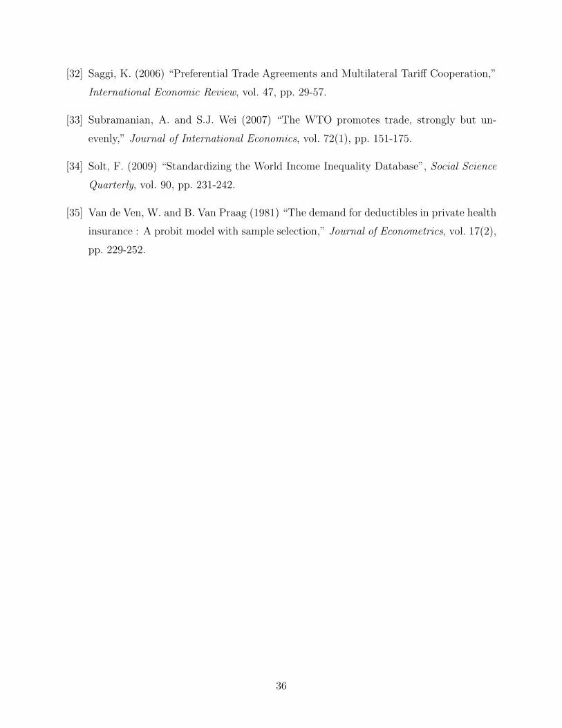
[32] Saggi, K. (2006) “Preferential Trade Agreements and Multilateral Tariff Cooperation,”
International Economic Review, vol. 47, pp. 29-57.
[33] Subramanian, A. and S.J. Wei (2007) “The WTO promotes trade, strongly but un-
evenly,” Journal of International Economics, vol. 72(1), pp. 151-175.
[34] Solt, F. (2009) “Standardizing the World Income Inequality Database”, Social Science
Quarterly, vol. 90, pp. 231-242.
[35] Van de Ven, W. and B. Van Praag (1981) “The demand for deductibles in private health
insurance : A probit model with sample selection,” Journal of Econometrics, vol. 17(2),
pp. 229-252.
36
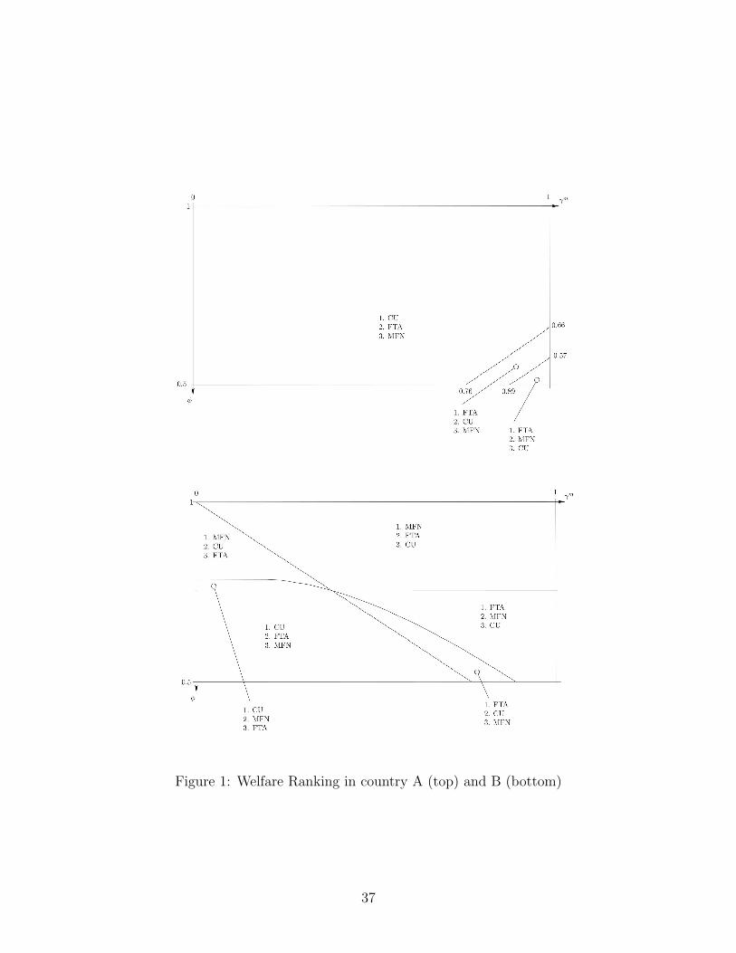
Figure 1: Welfare Ranking in country A (top) and B (bottom)
37
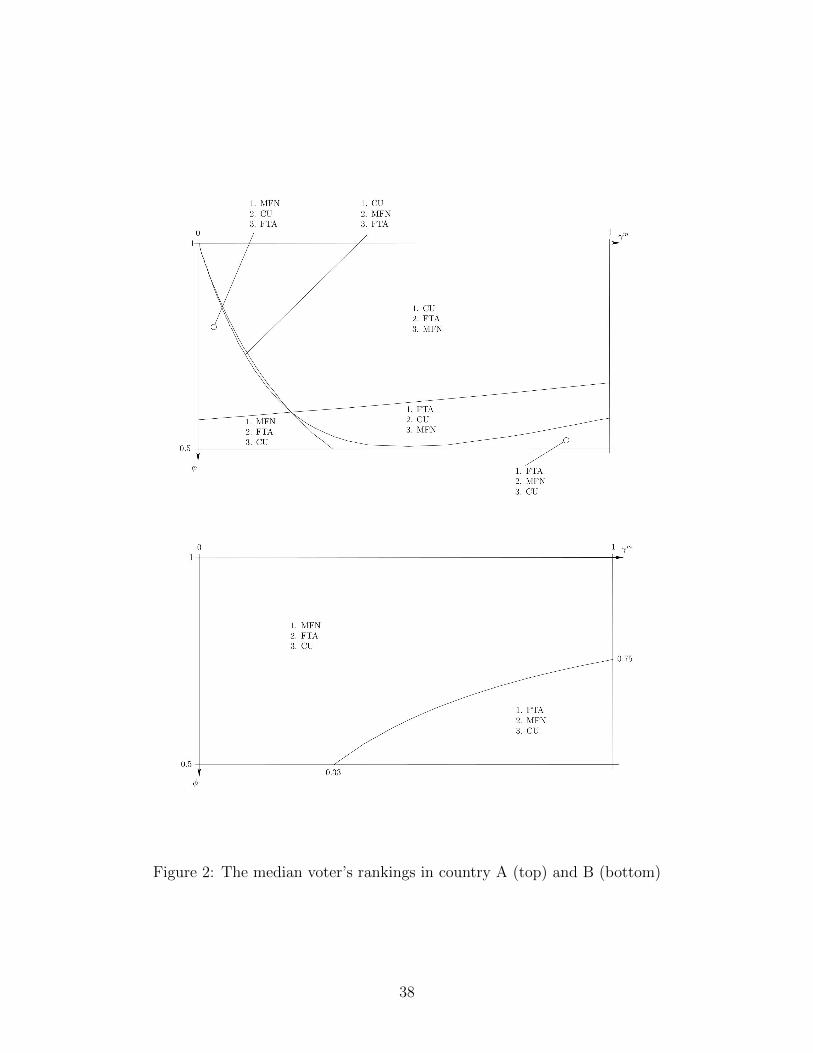
Figure 2: The median voter’s rankings in country A (top) and B (bottom)
38
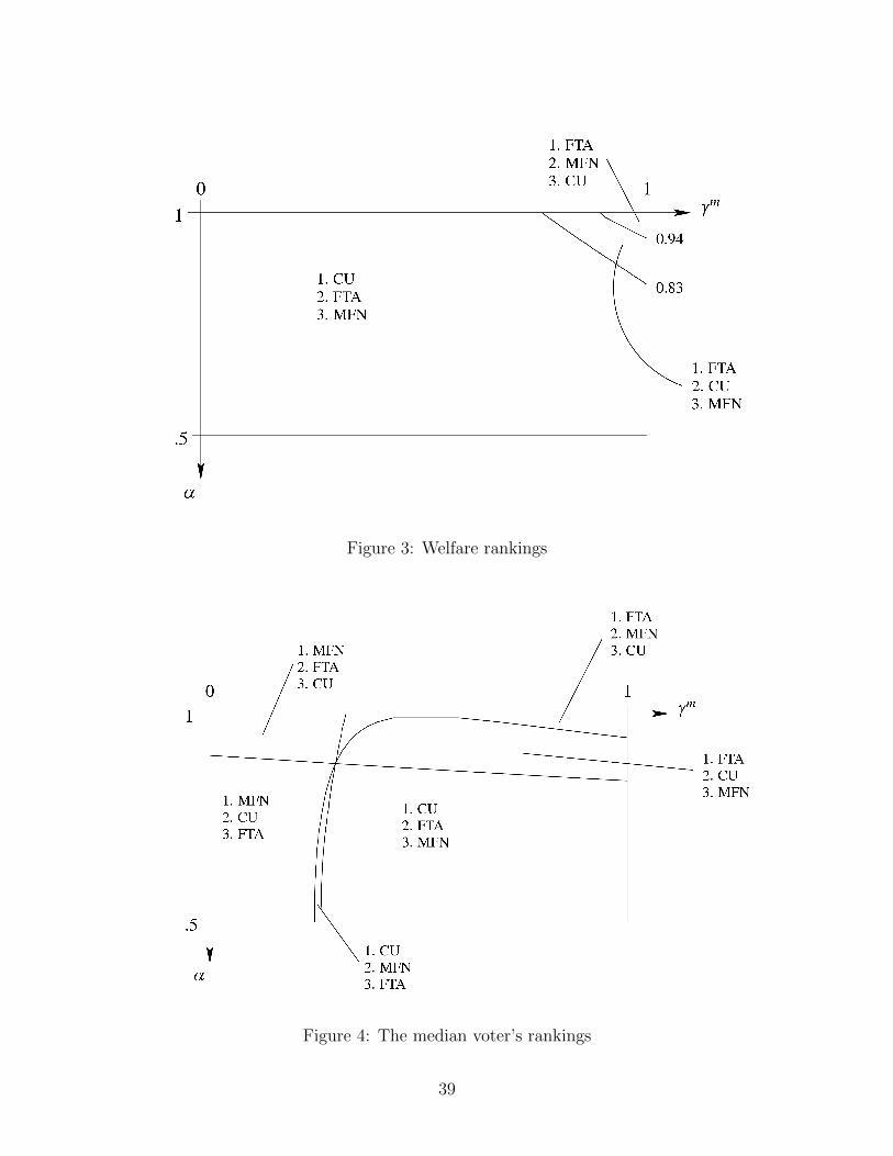
Figure 3: Welfare rankings
Figure 4: The median voter’s rankings
39
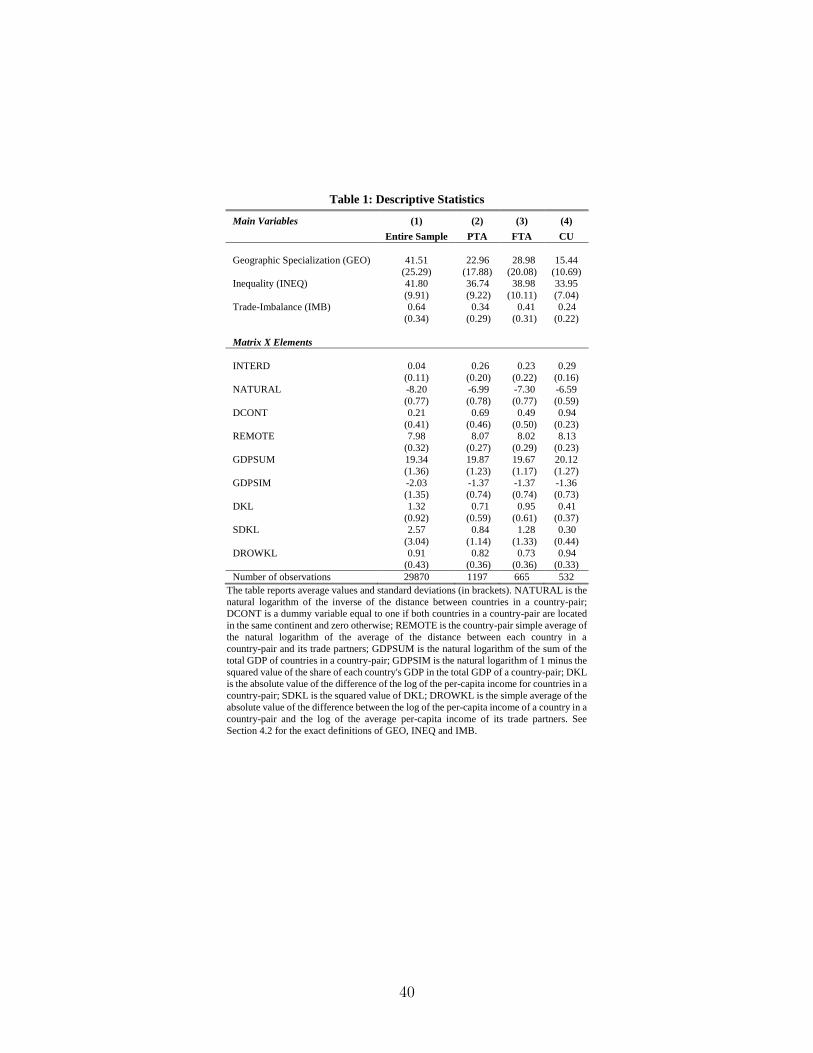
Table 1: Descriptive Statistics
Main Variables (1) (2) (3) (4)
Entire Sample PTA FTA CU
Geographic Specialization (GEO) 41.51 22.96 28.98 15.44
(25.29) (17.88) (20.08) (10.69)
Inequality (INEQ) 41.80 36.74 38.98 33.95
(9.91) (9.22) (10.11) (7.04)
Trade-Imbalance (IMB) 0.64 0.34 0.41 0.24
(0.34) (0.29) (0.31) (0.22)
Matrix X Elements
INTERD 0.04 0.26 0.23 0.29
(0.11) (0.20) (0.22) (0.16)
NATURAL -8.20 -6.99 -7.30 -6.59
(0.77) (0.78) (0.77) (0.59)
DCONT 0.21 0.69 0.49 0.94
(0.41) (0.46) (0.50) (0.23)
REMOTE 7.98 8.07 8.02 8.13
(0.32) (0.27) (0.29) (0.23)
GDPSUM 19.34 19.87 19.67 20.12
(1.36) (1.23) (1.17) (1.27)
GDPSIM -2.03 -1.37 -1.37 -1.36
(1.35) (0.74) (0.74) (0.73)
DKL 1.32 0.71 0.95 0.41
(0.92) (0.59) (0.61) (0.37)
SDKL 2.57 0.84 1.28 0.30
(3.04) (1.14) (1.33) (0.44)
DROWKL 0.91 0.82 0.73 0.94
(0.43) (0.36) (0.36) (0.33)
Number of observations 29870 1197 665 532
The table reports average values and standard deviations (in brackets). NATURAL is the
natural logarithm of the inverse of the distance between countries in a country-pair;
DCONT is a dummy variable equal to one if both countries in a country-pair are located
in the same continent and zero otherwise; REMOTE is the country-pair simple average of
the natural logarithm of the average of the distance between each country in a
country-pair and its trade partners; GDPSUM is the natural logarithm of the sum of the
total GDP of countries in a country-pair; GDPSIM is the natural logarithm of 1 minus the
squared value of the share of each country's GDP in the total GDP of a country-pair; DKL
is the absolute value of the difference of the log of the per-capita income for countries in a
country-pair; SDKL is the squared value of DKL; DROWKL is the simple average of the
absolute value of the difference between the log of the per-capita income of a country in a
country-pair and the log of the average per-capita income of its trade partners. See
Section 4.2 for the exact definitions of GEO, INEQ and IMB.
40
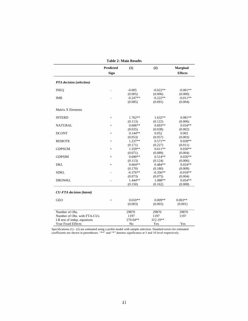
Table 2: Main Results
Predicted
Sign
(1) (2) Marginal
Effects
PTA decision (selection)
INEQ - -0.005 -0.022** -0.001**
(0.005) (0.006) (0.000)
IMB - -0.247** -0.222** -0.011**
(0.085) (0.091) (0.004)
Matrix X Elements
INTERD + 1.762** 1.632** 0.081**
(0.113) (0.122) (0.006)
NATURAL + 0.606** 0.693** 0.034**
(0.035) (0.038) (0.002)
DCONT + 0.144** 0.052 0.003
(0.053) (0.057) (0.003)
REMOTE + 1.237** 0.571** 0.028**
(0.171) (0.227) (0.011)
GDPSUM + 1.559** 0.611** 0.030**
(0.071) (0.089) (0.004)
GDPSIM + 0.690** 0.514** 0.026**
(0.113) (0.124) (0.006)
DKL + 0.604** 0.484** 0.024**
(0.170) (0.180) (0.009)
SDKL - -0.376** -0.356** -0.018**
(0.073) (0.075) (0.004)
DROWKL - 1.444** 1.088** 0.054**
(0.150) (0.162) (0.008)
CU-FTA decision (latent)
GEO + 0.010** 0.009** 0.003**
(0.003) (0.003) (0.001)
Number of Obs. 29870 29870 29870
Number of Obs. with FTA-CUs 1197 1197 1197
LR test of indep. equations 270.04** 312.19**
Year Fixed Effects No Yes Yes
Specifications (1) - (2) are estimated using a probit model with sample selection. Standard errors for estimated
coefficients are shown in parentheses. “**” and “*” denotes significance at 5 and 10 level respectively.
41
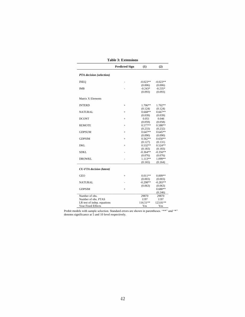
Table 3: Extensions
Predicted Sign (1) (2)
PTA decision (selection)
INEQ - -0.023** -0.023**
(0.006) (0.006)
IMB - -0.243* -0.235*
(0.093) (0.093)
Matrix X Elements
INTERD + 1.706** 1.702**
(0.124) (0.124)
NATURAL + 0.668** 0.667**
(0.039) (0.039)
DCONT + 0.051 0.046
(0.059) (0.058)
REMOTE + 0.577** 0.588**
(0.233) (0.232)
GDPSUM + 0.647** 0.645**
(0.090) (0.090)
GDPSIM + 0.562** 0.650**
(0.127) (0.131)
DKL + 0.532** 0.524**
(0.183) (0.183)
SDKL - -0.364** -0.356**
(0.076) (0.076)
DROWKL - 1.113** 1.099**
(0.165) (0.164)
CU-FTA decision (latent)
GEO + 0.011** 0.009**
(0.003) (0.003)
NATURAL - -0.298** -0.283**
(0.063) (0.063)
GDPSIM + 0.680**
(0.246)
Number of obs. 29870 29870
Number of obs. PTAS 1197 1197
LR test of indep. equations 116.51** 123.81**
Year Fixed Effects Yes Yes
Probit models with sample selection. Standard errors are shown in parentheses. “**” and “*”
denotes significance at 5 and 10 level respectively.
42
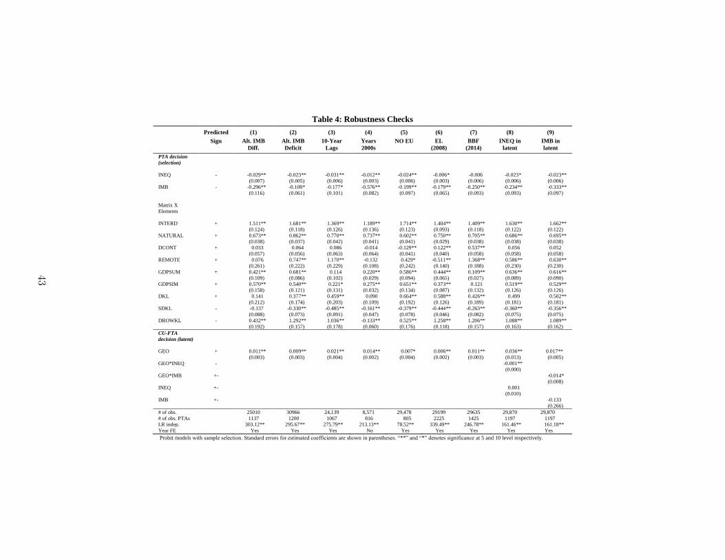
Table 4: Robustness Checks
Predicted
Sign
(1)
Alt. IMB
Diff.
(2)
Alt. IMB
Deficit
(3)
10-Year
Lags
(4)
Years
2000s
(5)
NO EU
(6)
EL
(2008)
(7)
BBF
(2014)
(8)
INEQ in
latent
(9)
IMB in
latent
PTA decision
(selection)
INEQ - -0.029** -0.023** -0.031** -0.012** -0.024** -0.006* -0.006 -0.023* -0.023**
(0.007) (0.005) (0.006) (0.003) (0.006) (0.003) (0.006) (0.006) (0.006)
IMB - -0.296** -0.108* -0.177* -0.576** -0.199** -0.179** -0.250** -0.234** -0.333**
(0.116) (0.061) (0.101) (0.082) (0.097) (0.065) (0.093) (0.093) (0.097)
Matrix X
Elements
INTERD + 1.511** 1.681** 1.369** 1.189** 1.714** 1.404** 1.409** 1.630** 1.662**
(0.124) (0.118) (0.126) (0.136) (0.123) (0.093) (0.118) (0.122) (0.122)
NATURAL + 0.673** 0.862** 0.770** 0.737** 0.602** 0.750** 0.705** 0.686** 0.695** (0.038) (0.037) (0.042) (0.041) (0.041) (0.029) (0.038) (0.038) (0.038)
DCONT + 0.033 0.064 0.086 -0.014 -0.129** 0.122** 0.537** 0.056 0.052
(0.057) (0.056) (0.063) (0.064) (0.041) (0.040) (0.058) (0.058) (0.058)
REMOTE + 0.076 0.747** 1.170** -0.132 0.429* -0.511** 1.368** 0.586** 0.630**
(0.261) (0.222) (0.229) (0.108) (0.242) (0.140) (0.188) (0.230) (0.230)
GDPSUM + 0.421** 0.681** 0.114 0.220** 0.586** 0.444** 0.109** 0.636** 0.616**
(0.109) (0.086) (0.102) (0.029) (0.094) (0.065) (0.027) (0.089) (0.090)
GDPSIM + 0.570** 0.540** 0.221* 0.275** 0.651** 0.373** 0.121 0.519** 0.529** (0.158) (0.121) (0.131) (0.032) (0.134) (0.087) (0.132) (0.126) (0.126)
DKL + 0.141 0.377** 0.459** 0.090 0.664** 0.588** 0.426** 0.499 0.502**
(0.212) (0.174) (0.203) (0.109) (0.192) (0.126) (0.189) (0.181) (0.181)
SDKL - -0.137 -0.330** -0.485** -0.161** -0.379** -0.444** -0.263** -0.360** -0.356**
(0.088) (0.073) (0.091) (0.047) (0.078) (0.046) (0.082) (0.075) (0.075)
DROWKL - 0.432** 1.292** 1.036** -0.133** 0.525** 1.258** 1.206** 1.088** 1.089**
(0.192) (0.157) (0.178) (0.060) (0.176) (0.118) (0.157) (0.163) (0.162)
CU-FTA
decision (latent)
GEO + 0.011** 0.009** 0.021** 0.014** 0.007* 0.006** 0.011** 0.036** 0.017**
(0.003) (0.003) (0.004) (0.002) (0.004) (0.002) (0.003) (0.013) (0.005)
GEO*INEQ - -0.001**
(0.000)
GEO*IMB +- -0.014*
(0.008) INEQ +- 0.001
(0.010)
IMB +- -0.133
(0.266)
# of obs. 25010 30966 24,139 8,571 29,478 29199 29635 29,870 29,870
# of obs. PTAs 1137 1200 1067 816 805 2225 1425 1197 1197
LR indep. 303.12** 295.67** 275.79** 213.13** 78.52** 339.49** 246.78** 161.46** 161.18**
Year FE Yes Yes Yes No Yes Yes Yes Yes Yes
Probit models with sample selection. Standard errors for estimated coefficients are shown in parentheses. “**” and “*” denotes significance at 5 and 10 level respectively.
43
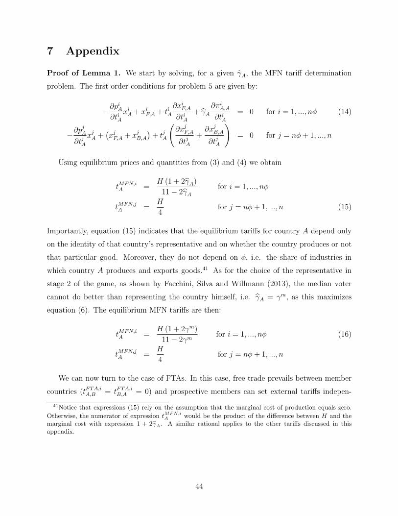
7 Appendix
Proof of Lemma 1. We start by solving, for a given γA, the MFN tariff determination
problem. The first order conditions for problem 5 are given by:
−∂piA
∂tiAxiA + xiF,A + tiA
∂xiF,A∂tiA
+ γA∂πiA,A∂tiA
= 0 for i = 1, ..., nφ (14)
−∂pjA
∂tjAxjA +
(xjF,A + xjB,A
)+ tjA
(∂xjF,A
∂tjA+∂xjB,A
∂tjA
)= 0 for j = nφ+ 1, ..., n
Using equilibrium prices and quantities from (3) and (4) we obtain
tMFN,iA =
H (1 + 2γA)
11− 2γAfor i = 1, ..., nφ
tMFN,jA =
H
4for j = nφ+ 1, ..., n (15)
Importantly, equation (15) indicates that the equilibrium tariffs for country A depend only
on the identity of that country’s representative and on whether the country produces or not
that particular good. Moreover, they do not depend on φ, i.e. the share of industries in
which country A produces and exports goods.41 As for the choice of the representative in
stage 2 of the game, as shown by Facchini, Silva and Willmann (2013), the median voter
cannot do better than representing the country himself, i.e. γA = γm, as this maximizes
equation (6). The equilibrium MFN tariffs are then:
tMFN,iA =
H (1 + 2γm)
11− 2γmfor i = 1, ..., nφ (16)
tMFN,jA =
H
4for j = nφ+ 1, ..., n
We can now turn to the case of FTAs. In this case, free trade prevails between member
countries (tFTA,iA,B = tFTA,iB,A = 0) and prospective members can set external tariffs indepen-
41Notice that expressions (15) rely on the assumption that the marginal cost of production equals zero.
Otherwise, the numerator of expression tMFN,iA would be the product of the difference between H and the
marginal cost with expression 1 + 2γA. A similar rational applies to the other tariffs discussed in thisappendix.
44
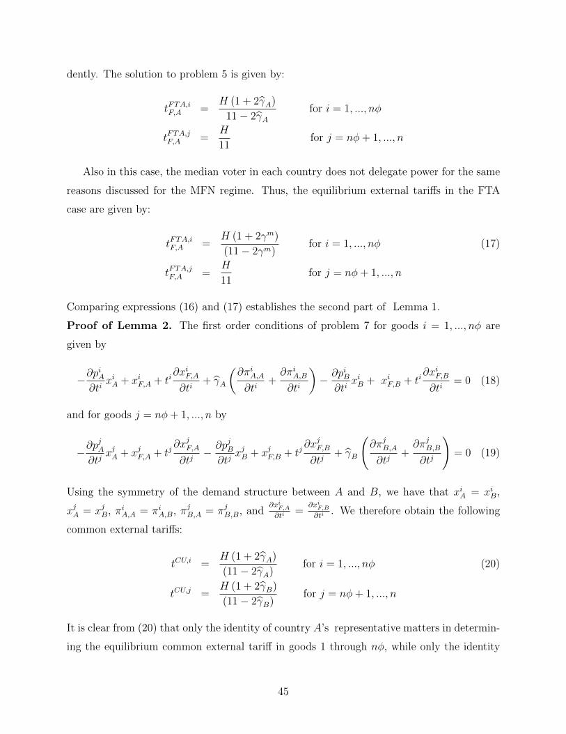
dently. The solution to problem 5 is given by:
tFTA,iF,A =H (1 + 2γA)
11− 2γAfor i = 1, ..., nφ
tFTA,jF,A =H
11for j = nφ+ 1, ..., n
Also in this case, the median voter in each country does not delegate power for the same
reasons discussed for the MFN regime. Thus, the equilibrium external tariffs in the FTA
case are given by:
tFTA,iF,A =H (1 + 2γm)
(11− 2γm)for i = 1, ..., nφ (17)
tFTA,jF,A =H
11for j = nφ+ 1, ..., n
Comparing expressions (16) and (17) establishes the second part of Lemma 1.
Proof of Lemma 2. The first order conditions of problem 7 for goods i = 1, ..., nφ are
given by
−∂piA
∂tixiA + xiF,A + ti
∂xiF,A∂ti
+ γA
(∂πiA,A∂ti
+∂πiA,B∂ti
)− ∂piB
∂tixiB + xiF,B + ti
∂xiF,B∂ti
= 0 (18)
and for goods j = nφ+ 1, ..., n by
−∂pjA
∂tjxjA + xjF,A + tj
∂xjF,A∂tj
− ∂pjB∂tj
xjB + xjF,B + tj∂xjF,B∂tj
+ γB
(∂πjB,A∂tj
+∂πjB,B∂tj
)= 0 (19)
Using the symmetry of the demand structure between A and B, we have that xiA = xiB,
xjA = xjB, πiA,A = πiA,B, πjB,A = πjB,B, and∂xiF,A
∂ti=
∂xiF,B
∂ti. We therefore obtain the following
common external tariffs:
tCU,i =H (1 + 2γA)
(11− 2γA)for i = 1, ..., nφ (20)
tCU,j =H (1 + 2γB)
(11− 2γB)for j = nφ+ 1, ..., n
It is clear from (20) that only the identity of country A’s representative matters in determin-
ing the equilibrium common external tariff in goods 1 through nφ, while only the identity
45
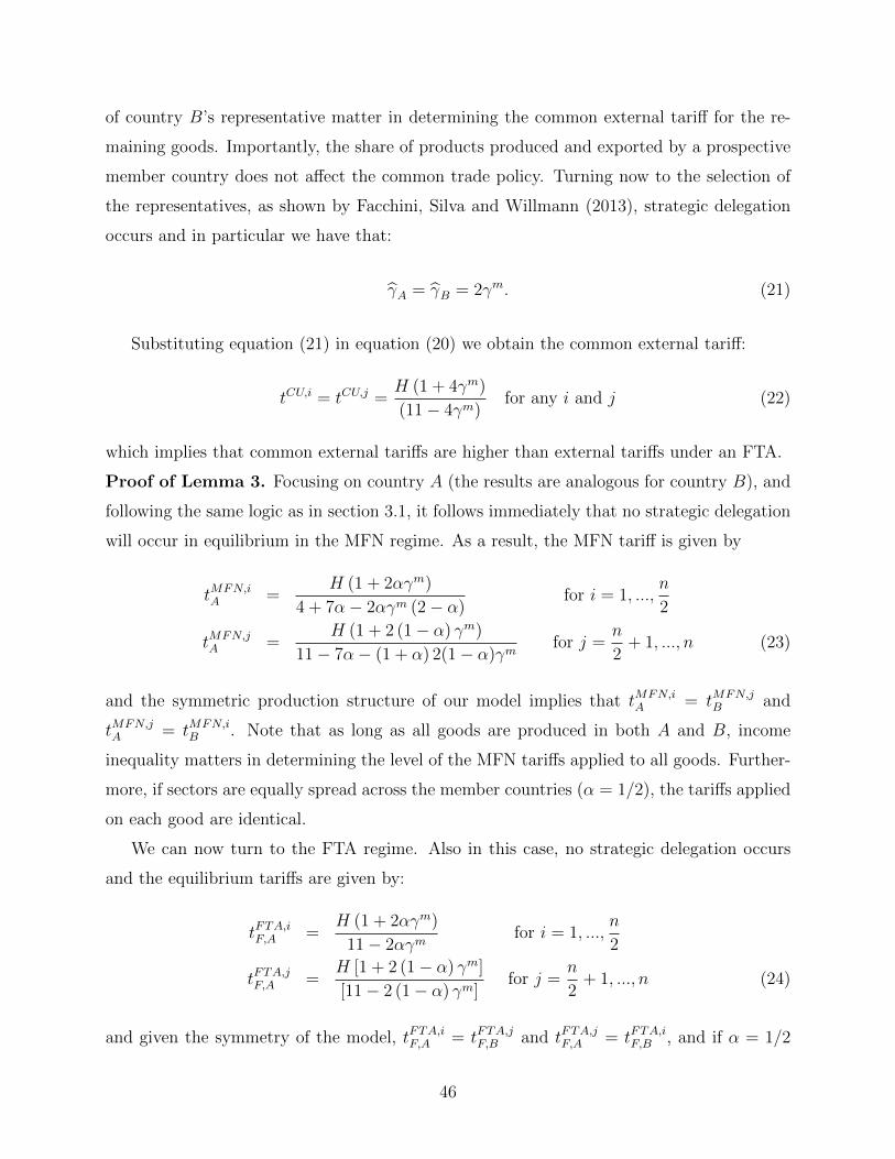
of country B’s representative matter in determining the common external tariff for the re-
maining goods. Importantly, the share of products produced and exported by a prospective
member country does not affect the common trade policy. Turning now to the selection of
the representatives, as shown by Facchini, Silva and Willmann (2013), strategic delegation
occurs and in particular we have that:
γA = γB = 2γm. (21)
Substituting equation (21) in equation (20) we obtain the common external tariff:
tCU,i = tCU,j =H (1 + 4γm)
(11− 4γm)for any i and j (22)
which implies that common external tariffs are higher than external tariffs under an FTA.
Proof of Lemma 3. Focusing on country A (the results are analogous for country B), and
following the same logic as in section 3.1, it follows immediately that no strategic delegation
will occur in equilibrium in the MFN regime. As a result, the MFN tariff is given by
tMFN,iA =
H (1 + 2αγm)
4 + 7α− 2αγm (2− α)for i = 1, ...,
n
2
tMFN,jA =
H (1 + 2 (1− α) γm)
11− 7α− (1 + α) 2(1− α)γmfor j =
n
2+ 1, ..., n (23)
and the symmetric production structure of our model implies that tMFN,iA = tMFN,j
B and
tMFN,jA = tMFN,i
B . Note that as long as all goods are produced in both A and B, income
inequality matters in determining the level of the MFN tariffs applied to all goods. Further-
more, if sectors are equally spread across the member countries (α = 1/2), the tariffs applied
on each good are identical.
We can now turn to the FTA regime. Also in this case, no strategic delegation occurs
and the equilibrium tariffs are given by:
tFTA,iF,A =H (1 + 2αγm)
11− 2αγmfor i = 1, ...,
n
2
tFTA,jF,A =H [1 + 2 (1− α) γm]
[11− 2 (1− α) γm]for j =
n
2+ 1, ..., n (24)
and given the symmetry of the model, tFTA,iF,A = tFTA,jF,B and tFTA,jF,A = tFTA,iF,B , and if α = 1/2
46
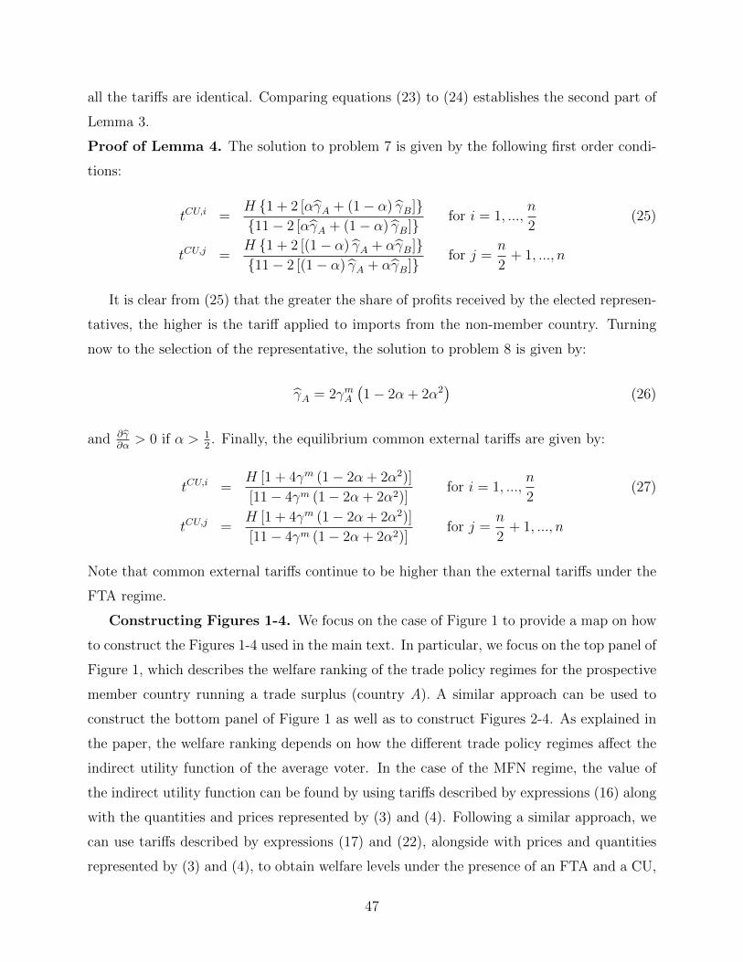
all the tariffs are identical. Comparing equations (23) to (24) establishes the second part of
Lemma 3.
Proof of Lemma 4. The solution to problem 7 is given by the following first order condi-
tions:
tCU,i =H {1 + 2 [αγA + (1− α) γB]}{11− 2 [αγA + (1− α) γB]}
for i = 1, ...,n
2(25)
tCU,j =H {1 + 2 [(1− α) γA + αγB]}{11− 2 [(1− α) γA + αγB]}
for j =n
2+ 1, ..., n
It is clear from (25) that the greater the share of profits received by the elected represen-
tatives, the higher is the tariff applied to imports from the non-member country. Turning
now to the selection of the representative, the solution to problem 8 is given by:
γA = 2γmA(1− 2α + 2α2
)(26)
and ∂γ∂α> 0 if α > 1
2. Finally, the equilibrium common external tariffs are given by:
tCU,i =H [1 + 4γm (1− 2α + 2α2)]
[11− 4γm (1− 2α + 2α2)]for i = 1, ...,
n
2(27)
tCU,j =H [1 + 4γm (1− 2α + 2α2)]
[11− 4γm (1− 2α + 2α2)]for j =
n
2+ 1, ..., n
Note that common external tariffs continue to be higher than the external tariffs under the
FTA regime.
Constructing Figures 1-4. We focus on the case of Figure 1 to provide a map on how
to construct the Figures 1-4 used in the main text. In particular, we focus on the top panel of
Figure 1, which describes the welfare ranking of the trade policy regimes for the prospective
member country running a trade surplus (country A). A similar approach can be used to
construct the bottom panel of Figure 1 as well as to construct Figures 2-4. As explained in
the paper, the welfare ranking depends on how the different trade policy regimes affect the
indirect utility function of the average voter. In the case of the MFN regime, the value of
the indirect utility function can be found by using tariffs described by expressions (16) along
with the quantities and prices represented by (3) and (4). Following a similar approach, we
can use tariffs described by expressions (17) and (22), alongside with prices and quantities
represented by (3) and (4), to obtain welfare levels under the presence of an FTA and a CU,
47
respectively.
First, we need to compare welfare comparison under the FTA and CU regimes, while
the other two comparisons consider each PTA against the MFN regime. Each comparison
involves taking the difference between the indirect utility function of the average voter be-
tween two trade regimes. This implies that the welfare comparison between an FTA and
a CU uses the difference between the value of the indirect utility function for the average
voter under these trade regimes, i.e. v(tFTA, γA
)− v
(tCU , γA
). A similar strategy applies
to the other two welfare comparisons. As can be seen from Figure 1, the difference in welfare
levels between trade regimes depends on the parameters capturing the degree of bilateral
trade imbalance (φ) and the degree of income inequality (γm).42 We proceed by varying the
parameter capturing the degree of trade imbalance (vertical axis) between 0.5 and 1.0 using
0.01 incremental values, and then calculate, for each value of this parameter, the threshold
in terms of the degree of income inequality (horizontal axis) needed to set the difference in
welfare level between the two trade regimes to zero. The table below shows the thresholds
for the three pair-wise welfare comparisons:
[Table A2 – Welfare Ranking]
In line with the top panel of Figure 1, the information provided by Table A2 indicates
that, in the presence of a balanced distribution of market access (φ = 0.5), the FTA welfare
dominates the CU if inequality is sufficiently low (γm > 0.76) as indicated by column 1.
Similarly, the presence of balanced bilateral trade also implies that a CU welfare dominates
the MFN regime if the degree of income inequality is sufficiently low (γm > 0.89) as indicated
by column 2. As we move up along the vertical axis, towards a more unequal distribution of
market access, we notice from Table A2 that the threshold indicating the degree of income
inequality needed so that the FTA (CU) welfare dominates the CU (MFN) also rises, implying
increasing values for the parameter γm. We can then conclude that above a certain degree of
unbalanced market access, the CU regime welfare dominates the FTA regime (φ > 0.66) as
well as the MFN regime (φ > 0.57). Varying the degree of trade imbalances allows us then
to derive the two lines found in the bottom right corner of Figure 1, separating areas where
the average voter prefers the CU regime over the FTA regime (and vice-versa), as well as
42In general, the sign of the difference between the value of the indirect utility functions does not dependon H since this parameter multiplies all other terms of these expressions.
48
separating areas where the average voter either prefers the CU regime or the MFN regime.
In line with Figure 1, the FTA regime welfare dominates the MFN regime regardless of the
level of income inequality according to column 3 of Table 5.
The bottom panel of Figure 1 follows the same approach used in the top panel of that
figure while focusing on the case of the country running a bilateral trade deficit (country B).
In the case of Figure 2, we use similar approach but the trade regime comparison relies on
the indirect utility function of the median (rather than the average) voter since we consider
the political viability of trade agreements in that case. Similarly, Figures 3 and 4 follow the
approach used in Figures 1 and 2, respectively. The only difference between these two groups
of figures is that Figures 3 and 4 rely on setting different values of the degree of geographic
specialization (α) in order to obtain the threshold of the parameter measuring the degree of
income inequality (γm) since we assume the presence of balanced trade in Figures 3 and 4.
49
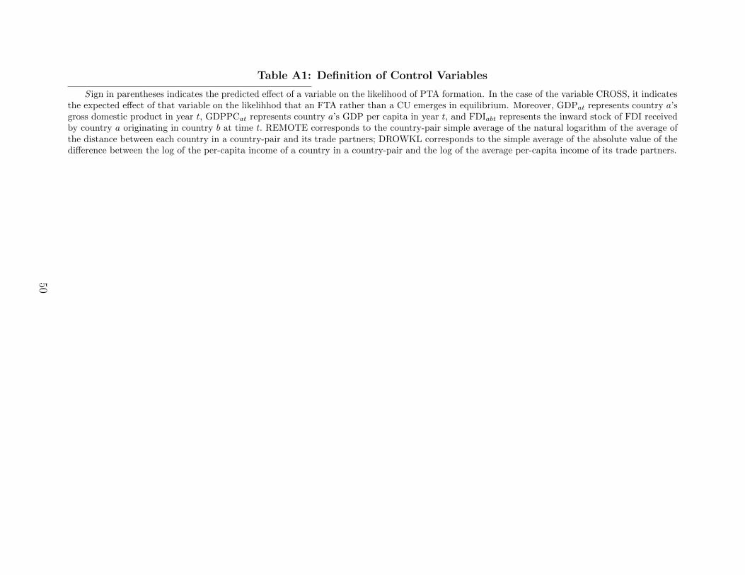
Table A1: Definition of Control Variables
S ign in parentheses indicates the predicted effect of a variable on the likelihood of PTA formation. In the case of the variable CROSS, it indicatesthe expected effect of that variable on the likelihhod that an FTA rather than a CU emerges in equilibrium. Moreover, GDPat represents country a’sgross domestic product in year t, GDPPCat represents country a’s GDP per capita in year t, and FDIabt represents the inward stock of FDI receivedby country a originating in country b at time t. REMOTE corresponds to the country-pair simple average of the natural logarithm of the average ofthe distance between each country in a country-pair and its trade partners; DROWKL corresponds to the simple average of the absolute value of thedifference between the log of the per-capita income of a country in a country-pair and the log of the average per-capita income of its trade partners.
50
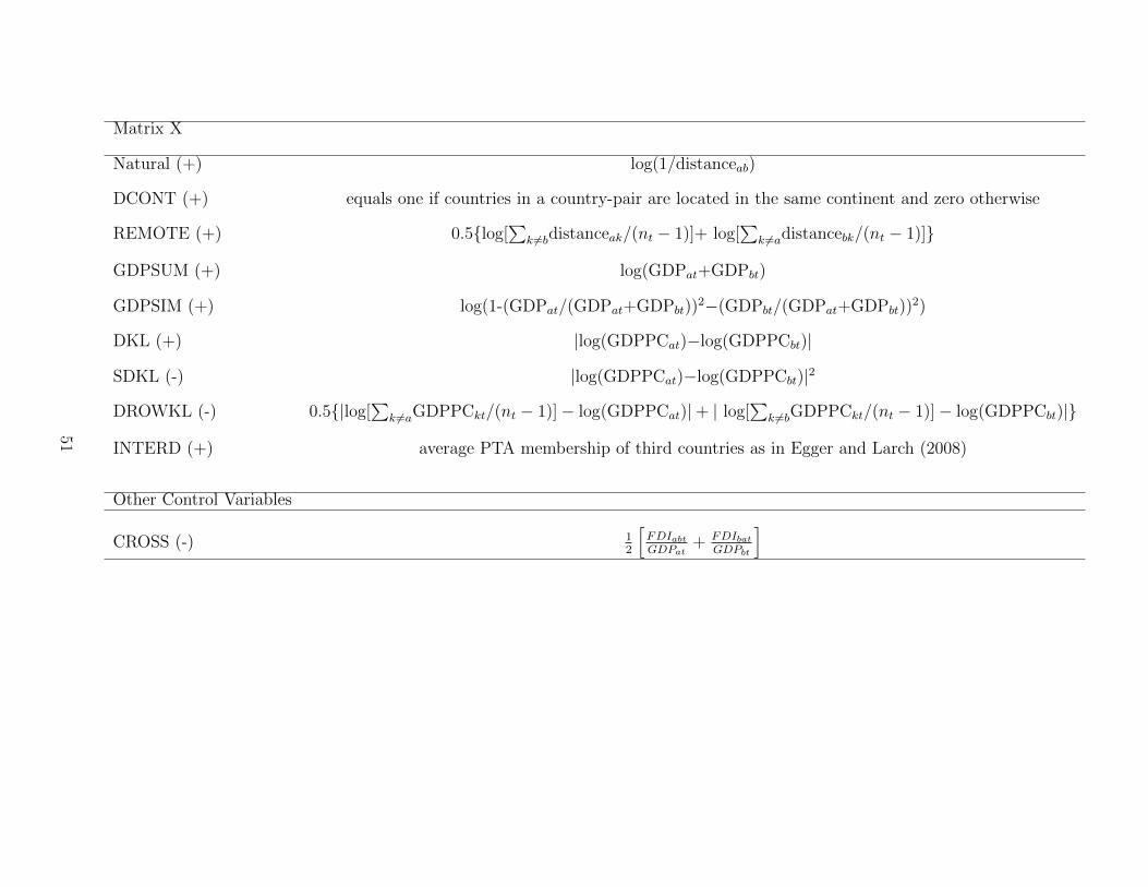
Matrix X
Natural (+) log(1/distanceab)
DCONT (+) equals one if countries in a country-pair are located in the same continent and zero otherwise
REMOTE (+) 0.5{log[∑
k 6=bdistanceak/(nt − 1)]+ log[∑
k 6=adistancebk/(nt − 1)]}
GDPSUM (+) log(GDPat+GDPbt)
GDPSIM (+) log(1-(GDPat/(GDPat+GDPbt))2−(GDPbt/(GDPat+GDPbt))
2)
DKL (+) |log(GDPPCat)−log(GDPPCbt)|
SDKL (-) |log(GDPPCat)−log(GDPPCbt)|2
DROWKL (-) 0.5{|log[∑
k 6=aGDPPCkt/(nt − 1)]− log(GDPPCat)|+ | log[∑
k 6=bGDPPCkt/(nt − 1)]− log(GDPPCbt)|}
INTERD (+) average PTA membership of third countries as in Egger and Larch (2008)
Other Control Variables
CROSS (-) 12
[FDIabtGDPat
+ FDIbatGDPbt
]
51