Embed Size (px)
Citation preview
HAL Id: hal-00020066https://hal.archives-ouvertes.fr/hal-00020066
Submitted on 3 Mar 2006
HAL is a multi-disciplinary open accessarchive for the deposit and dissemination of sci-entific research documents, whether they are pub-lished or not. The documents may come fromteaching and research institutions in France orabroad, or from public or private research centers.
L’archive ouverte pluridisciplinaire HAL, estdestinée au dépôt et à la diffusion de documentsscientifiques de niveau recherche, publiés ou non,émanant des établissements d’enseignement et derecherche français ou étrangers, des laboratoirespublics ou privés.
The pharmacophore kernel for virtual screening withsupport vector machines
Pierre Mahé, Liva Ralaivola, Véronique Stoven, Jean-Philippe Vert
To cite this version:Pierre Mahé, Liva Ralaivola, Véronique Stoven, Jean-Philippe Vert. The pharmacophore kernel forvirtual screening with support vector machines. 2006. <hal-00020066>

ccsd
-000
2006
6, v
ersi
on 1
- 3
Mar
200
6
The pharmacophore kernel for virtual screening with support vectormachines
Pierre MaheCenter for Computational Biology
Ecole des Mines de [email protected]
Liva RalaivolaLaboratoire d’Informatique Fondamentale
University Provence/Aix-Marseille [email protected]
Veronique StovenCenter for Computational Biology
Ecole des Mines de [email protected]
Jean-Philippe VertCenter for Computational Biology
Ecole des Mines de [email protected]
March 3, 2006
Abstract
We introduce a family of positive definite kernels specifically optimized for the manipulation of 3D structuresof molecules with kernel methods. The kernels are based on the comparison of the three-points pharmacophorespresent in the 3D structures of molecules, a set of molecularfeatures known to be particularly relevant for virtualscreening applications. We present a computationally demanding exact implementation of these kernels, as well asfast approximations related to the classical fingerprint-based approaches. Experimental results suggest that this newapproach outperforms state-of-the-art algorithms based on the 2D structure of molecules for the detection of inhibitorsof several drug targets.
1 Introduction
Virtual screening refers to the process of inferring biological properties of moleculesin silico, and plays an increas-ingly important role at the early stages of the drug discovery process to select candidate molecules with promisingdrug-likeness, including good toxicity and pharmacokinetics properties, as well as the potential to bind and inhibit atarget protein of interest (1). In this context, structure-activity relationship (SAR) analysis is commonly used to buildpredictive models for the property of interest from a description of the molecules, using statistical procedures to buildthese models from the analysis of molecules with known properties (2).
It is widely accepted that several drug-like properties canbe efficiently deduced from the 2D structure of themolecule, that is, the description of a molecule as a set of atoms and their covalent bonds. For example, Lipinski’s“rule of five” remains a widely used standard for the prediction of intestinal absorption (3), and the prediction ofmutagenicity from 2D molecular fragments is an accurate state-of-the-art approach (4). In the case of target bindingprediction, however, the molecular mechanisms responsible for the binding are known to depend on a precise 3Dcomplementarity between the drug and the target, from both the steric and electrostatic perspectives (5). For thisreason, there has been a long history of research on the prediction of these interactions from the 3D representation ofmolecules, that is, their spatial conformation in the 3D space. If the 3D structure of the target is known, the strengthof the interaction can be directly evaluated by docking techniques, that quantify the complementarity of the moleculeto the target in terms of energy (6). In the general case wherethe 3D structure of the target is unknown, however, thedocking approach is not possible anymore and the modeler must resort to creating a predictive model from availabledata, typically a pool of molecules with known affinity to thetarget; this approach is usually referred to as theligand-basedapproach to virtual screening.
Most approaches to ligand-based virtual screening requireto represent and compare 3D structures of molecules.The comparison of 3D structures can for example rely on optimal alignments in the 3D space (7), or on the comparison
1
no separating hyperplane one possible separating hyperplane separating surface
input space Xφ
feature space H input space X
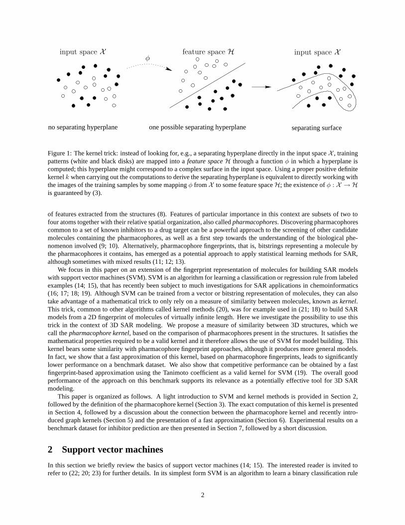
Figure 1: The kernel trick: instead of looking for, e.g., a separating hyperplane directly in the input spaceX , trainingpatterns (white and black disks) are mapped into afeature spaceH through a functionφ in which a hyperplane iscomputed; this hyperplane might correspond to a complex surface in the input space. Using a proper positive definitekernelk when carrying out the computations to derive the separatinghyperplane is equivalent to directly working withthe images of the training samples by some mappingφ fromX to some feature spaceH; the existence ofφ : X → His guaranteed by (3).
of features extracted from the structures (8). Features of particular importance in this context are subsets of two tofour atoms together with their relative spatial organization, also calledpharmacophores. Discovering pharmacophorescommon to a set of known inhibitors to a drug target can be a powerful approach to the screening of other candidatemolecules containing the pharmacophores, as well as a first step towards the understanding of the biological phe-nomenon involved (9; 10). Alternatively, pharmacophore fingerprints, that is, bitstrings representing a molecule bythe pharmacophores it contains, has emerged as a potential approach to apply statistical learning methods for SAR,although sometimes with mixed results (11; 12; 13).
We focus in this paper on an extension of the fingerprint representation of molecules for building SAR modelswith support vector machines (SVM). SVM is an algorithm for learning a classification or regression rule from labeledexamples (14; 15), that has recently been subject to much investigations for SAR applications in chemoinformatics(16; 17; 18; 19). Although SVM can be trained from a vector or bitstring representation of molecules, they can alsotake advantage of a mathematical trick to only rely on a measure of similarity between molecules, known askernel.This trick, common to other algorithms called kernel methods (20), was for example used in (21; 18) to build SARmodels from a 2D fingerprint of molecules of virtually infinite length. Here we investigate the possibility to use thistrick in the context of 3D SAR modeling. We propose a measure of similarity between 3D structures, which wecall thepharmacophore kernel, based on the comparison of pharmacophores present in the structures. It satisfies themathematical properties required to be a valid kernel and ittherefore allows the use of SVM for model building. Thiskernel bears some similarity with pharmacophore fingerprint approaches, although it produces more general models.In fact, we show that a fast approximation of this kernel, based on pharmacophore fingerprints, leads to significantlylower performance on a benchmark dataset. We also show that competitive performance can be obtained by a fastfingerprint-based approximation using the Tanimoto coefficient as a valid kernel for SVM (19). The overall goodperformance of the approach on this benchmark supports its relevance as a potentially effective tool for 3D SARmodeling.
This paper is organized as follows. A light introduction to SVM and kernel methods is provided in Section 2,followed by the definition of the pharmacophore kernel (Section 3). The exact computation of this kernel is presentedin Section 4, followed by a discussion about the connection between the pharmacophore kernel and recently intro-duced graph kernels (Section 5) and the presentation of a fast approximation (Section 6). Experimental results on abenchmark dataset for inhibitor prediction are then presented in Section 7, followed by a short discussion.
2 Support vector machines
In this section we briefly review the basics of support vectormachines (14; 15). The interested reader is invited torefer to (22; 20; 23) for further details. In its simplest form SVM is an algorithm to learn a binary classification rule
2

from a set of labeled examples. More formally, suppose one isgiven a set of examples with a binary label attached toeach example, that is, a setS = {(x1, y1), . . . , (xℓ, yℓ)} where(xi, yi) ∈ X × {−1, +1} for i = 1, . . . , ℓ. HereX isan inner-product space (e.g.R
d), equipped with inner product〈·, ·〉, that represents the space of data to be analyzed,typically molecules represented byd-dimensional fingerprints, and the labels+1 and−1 are meant to represent twoclasses of objects, such as inhibitors or non-inhibitors ofa target of interest. The purpose of SVM is to learn fromS aclassification functionf : X → {−1, +1} that can be used to predict the class of new unlabeled examplesx asf(x).
In the case of SVM, the classification function is simply of the form f(x) = sign(〈w, x〉 + b), where sign(·)is the function returning the sign,+1 or −1, of its argument. Geometrically speaking, this means thatf outputs aprediction for a patternx depending upon which side of the hyperplane〈w, x〉 + b = 0 it falls in. More precisely,SVM learn a separating hyperplane fromS defined by a vectorw that is a linear combination of the training vectorsw =
∑ℓ
i=1 αixi, for someαi ∈ R, i = 1, . . . , ℓ, obtained by solving a linearly constrained quadratic problem meant tooptimize a trade-off between finding a hyperplane that correctly separates all the points, while being as far as possiblefrom each point. The linear classifierf can consequently be rewritten as
f(x) = sign
(
ℓ∑
i=1
αi〈xi, x〉 + b
)
. (1)
However, when dealing with nonlinearly separable problems, such as the one depicted on Figure 1 (left), the setof linear classifiers may not be rich enough to provide a good classification function, no matter what the values of theparametersw ∈ X andb ∈ R are. The purpose of thekernel trick(24; 14), is precisely to overcome this limitationby applying a linear approach to the transformed dataφ(x1), . . . , φ(xℓ) rather than the original data, whereφ is anembedding from the input spaceX to the feature spaceH, usually, but not necessarily, a high-dimensional space,equipped with dot product〈·, ·〉H. Thus, according to (1), the separating functionf writes as
f(x) = sign
(
ℓ∑
i=1
αi〈φ(xi), φ(x)〉H + b
)
. (2)
The key ingredient in the kernel approach is to replace the dot product inH with a kernel, using the definition ofpositive definite kernels.
Definition 1 (Positive definite kernel). LetX be a nonempty space. LetK : X × X → R be a symmetric function.K is said to be a positive definite kernel if and only if, for allℓ ∈ N, for all x1, . . . , xℓ ∈ X , the squareℓ × ℓ matrixK = (K(xi, xj))1≤i,j≤ℓ is positive semi-definite, that is, all its eigenvalues are nonnegative.
For a given setSx = {x1, . . . , xℓ}, K is theGram matrixof K with respect toSx. A fundamental property ofpositive definite kernels that underlies the kernel trick isthe fact that each such kernel can be represented as an innerproduct in some space. More precisely, it can be shown (25) that for any positive definite kernel functionK, thereexists a spaceH, equipped with the inner product〈·, ·〉H, and a mappingφ : X → H such that:
∀u, v ∈ X K(u, v) = 〈φ(u), φ(v)〉H . (3)
The kernel trick consists in replacing all occurrences of〈·, ·〉H in (2) by a positive definite kernelK such that thecorresponding decision functionf , for an input patternx, is given by:
f(x) = sign
(
ℓ∑
i=1
αiK(xi, x) + b
)
. (4)
For SVM as well as for other kernel methods, the knowledge of the Gram matrix suffices to obtain the coefficientsαi.For any given positive definite kernel, applying the kernel trick turns out to be equivalent to transforming the
input patternsx1, . . . , xℓ into the corresponding vectorsφ(x1), . . . , φ(xℓ) ∈ H and to look for hyperplanes inH,as illustrated in Figure 1 (middle). The decision surface ininput spaceX corresponding to the selected separatinghyperplane inH might be quite complex (see Figure 1, right).
A noteworthy feature of support vector machines and more generally of kernel methods (23) is that, since ready-to-use libraries to derive separating hyperplanes are available, the only requirement for them to be applied to a specificclassification problem is to have at hand a proper kernel function to assess the similarity between patterns of the inputspace considered. Henceforth, their use actually fit in the framework of classification problems involving structureddata such as chemical compounds, provided some kernel function has been derived. The rest of the paper is devotedto the construction and analysis of such a kernel for 3D structures of molecules.
3
2
d1
d3
d
O
O
2
d1
d3
d
O
O
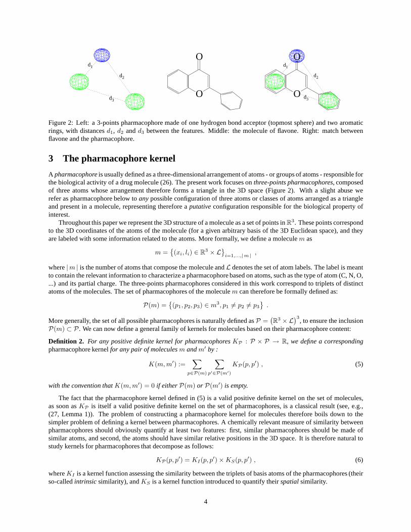
Figure 2: Left: a 3-points pharmacophore made of one hydrogen bond acceptor (topmost sphere) and two aromaticrings, with distancesd1, d2 andd3 between the features. Middle: the molecule of flavone. Right: match betweenflavone and the pharmacophore.
3 The pharmacophore kernel
A pharmacophoreis usually defined as a three-dimensional arrangement of atoms - or groups of atoms - responsible forthe biological activity of a drug molecule (26). The presentwork focuses onthree-points pharmacophores, composedof three atoms whose arrangement therefore forms a trianglein the 3D space (Figure 2). With a slight abuse werefer as pharmacophore below toanypossible configuration of three atoms or classes of atoms arranged as a triangleand present in a molecule, representing therefore aputativeconfiguration responsible for the biological property ofinterest.
Throughout this paper we represent the 3D structure of a molecule as a set of points inR3. These points correspondto the 3D coordinates of the atoms of the molecule (for a givenarbitrary basis of the 3D Euclidean space), and theyare labeled with some information related to the atoms. Moreformally, we define a moleculem as
m ={
(xi, li) ∈ R3 × L
}
i=1,...,|m |,
where|m | is the number of atoms that compose the molecule andL denotes the set of atom labels. The label is meantto contain the relevant information to characterize a pharmacophore based on atoms, such as the type of atom (C, N, O,...) and its partial charge. The three-points pharmacophores considered in this work correspond to triplets of distinctatoms of the molecules. The set of pharmacophores of the moleculem can therefore be formally defined as:
P(m) ={
(p1, p2, p3) ∈ m3, p1 6= p2 6= p3
}
.
More generally, the set of all possible pharmacophores is naturally defined asP =(
R3 × L
)3, to ensure the inclusion
P(m) ⊂ P . We can now define a general family of kernels for molecules based on their pharmacophore content:
Definition 2. For any positive definite kernel for pharmacophoresKP : P × P → R, we define a correspondingpharmacophore kernelfor any pair of moleculesm andm′ by :
K(m, m′) :=∑
p∈P(m)
∑
p′∈P(m′)
KP(p, p′) , (5)
with the convention thatK(m, m′) = 0 if eitherP(m) or P(m′) is empty.
The fact that the pharmacophore kernel defined in (5) is a valid positive definite kernel on the set of molecules,as soon asKP is itself a valid positive definite kernel on the set of pharmacophores, is a classical result (see, e.g.,(27, Lemma 1)). The problem of constructing a pharmacophorekernel for molecules therefore boils down to thesimpler problem of defining a kernel between pharmacophores. A chemically relevant measure of similarity betweenpharmacophores should obviously quantify at least two features: first, similar pharmacophores should be made ofsimilar atoms, and second, the atoms should have similar relative positions in the 3D space. It is therefore natural tostudy kernels for pharmacophores that decompose as follows:
KP(p, p′) = KI(p, p′) × KS(p, p′) , (6)
whereKI is a kernel function assessing the similarity between the triplets of basis atoms of the pharmacophores (theirso-calledintrinsic similarity), andKS is a kernel function introduced to quantify theirspatialsimilarity.
4
We can furthermore investigate intrinsic and spatial kernels that factorize themselves as products of more basickernels between atoms and pairwise distances, respectively. Triplets of atoms are indeed globally similar if the threecorresponding pairs of atoms are simultaneously similar, and triangles are similar if the lengths of their edges arepairwise similar. For any pair of pharmacophoresp = ((xi, li))i=1,2,3 andp′ = ((x′
i, l′i))i=1,2,3, this suggests to
define kernels as follows:
KI(p, p′) =
3∏
i=1
KFeat (li, l′i) , (7)
KS(p, p′) =
3∏
i=1
KDist
(
‖ xi − xi+1 ‖, ‖ x′i − x′
i+1 ‖)
, (8)
where‖ . ‖ denotes the Euclidean distance, the indicesi are taken modulo 3, andKFeat andKDist are kernels functionsintroduced to compare pairs of labels fromL, and pairs of distances, respectively. It suffices now to define the kernelsKFeat on L × L and KDist on R × R in order to obtain, by (5), (6), (7) and (8), a pharmacophore kernel formolecules. The first one compares the atom labels, while the second compares the distances between atoms in thepharmacophores. Intuitively they define the basic notions of similarity involved in the pharmacophore comparison,which in turns defines the overall similarity between molecules.
The kernel we use forKDist is the Gaussian radial basis function (RBF) kernel, known tobe a safe default choicefor SVM working on real numbers or vectors (20):
KRBFDist (x, y) = exp
(
−||x − y||2
2σ2
)
, (9)
whereσ > 0 is the bandwith parameter that will be optimized as part of the training of the classifier (see Section 7.2).Concerning the kernelKFeat between labels, we investigate several choices. The labelsbelonging in principle to
a finite set of possible labels, e.g., the set of atom types with their charges (C, C+, C−, N, ...), the followingDirackernelis a natural default choice to compare a pair of atom labelsl, l′ ∈ L :
KDiracFeat (l, l′) =
{
1 if l = l′ ,
0 otherwise.(10)
Alternatively, it might be relevant for pharmacophore definition to compare atoms not only on the basis of theirtypes and partial charges, but also in terms of other physicochemical parameters such as their size, polarity andelectronegativity. Formally, a physicochemical parameter for an atom with labell is a real numberf(l). In that case,the Gaussian RBF kernel (9) could be applied directly to the parameter values to compare labels. A practical drawbackof this kernel, however, is that it never vanishes. This induces an important computational burden compared to theDirac kernel (see Section 4). As a result, we prefer to use therelatedtriangular kernel:
KTriFeat(l, l
′) =
{
C−||f(l)−f(l′)||C
if ||f(l) − f(l′)|| ≤ C ,
0 otherwise.(11)
An important difference between the Gaussian RBF and triangular kernels lies in the fact that the triangular kernelhas a compact support, which means that it can be equal to0 for different atoms, resulting in important computationalgain. The parameterC, to be optimized during the training phase of the algorithm,represents the range beyond whichthe kernel vanishes.
Note finally that the Gaussian RBF (9), triangular (11), and Dirac (10) kernels are known to be positive definite(20), and it follows from the closure properties of the family of kernel functions, that the kernel between pharma-cophoresKP is valid for any choice of the kernelsKDist andKFeat proposed above.
4 Kernel computation
We are now left with the task of computing the pharmacophore kernel (5) for a particular choice of feature and distancekernelsKFeat andKDist. In this section we provide a simple analytical formula for this computation.
5

For any pair of moleculesm ={
(xi, li) ∈ R3 × L
}
i=1,...,|m|andm′ =
{
(x′i, l
′i) ∈ R
3 × L}
i=1,...,|m′|, let us
define a square matrixM of sizen = |m| × |m′|, whose dimensions are indexed by the Cartesian product ofm andm′. In other words, to each indexi ∈ [1, n] corresponds a unique couple of indices(i1, i2) ∈ [1, |m|] × [1, |m′|], andto each dimension of the matrixM corresponds a distinct pair of points taken from the moleculesm andm′. Denotingby 1 (.) the indicator function equal to one if its argument is true, zero otherwise, the entries ofM are defined by:
M [i, j] = M [(i1, i2), (j1, j2)]
= KFeat
(
li1 , l′i2
)
× KDist
(
||xi1 − xj1 ||, ||x′i2− x′
j2||)
× 1 (i1 6= j1) × 1 (i2 6= j2) . (12)
The value of the pharmacophore kernel betweenm andm′ can now be deduced from the matrixM by the followingresult:
Proposition 1. The pharmacophore kernel (5) between a pair of moleculesm andm′ is equal to:
K(m, m′) = trace(M3) ,
whereM is the square matrix of dimension|m | × |m′ | constructed fromm andm′ by (12).
Proof. Developing the matrix products involved in the expression of M3 we get
trace(M3) =
n∑
i,j,k=1
M [i, j]M [j, k]M [k, i] ,
wheren = |m| × |m′| is the size ofM . Using the fact that the indices ofM ranges over the Cartesian product of theset of indices[1, |m|] and[1, |m′|], we can rewrite this expression as :
trace(M3) =
|m|∑
i1,j1,k1=1
|m′|∑
i2,j2,k2=1
M [(i1, i2), (j1, j2)]M [(j1, j2), (k1, k2)]M [(k1, k2), (i1, i2)] .
Substituting with the definition ofM given in (12), we obtain :
trace(M3) =
|m|∑
i1,j1,k1=1
|m′|∑
i2,j2,k2=1
1 (i1 6= j1)1 (j1 6= k1)1 (k1 6= i1) × 1 (i2 6= j2)1 (j2 6= k2)1 (k2 6= i2)
×KFeat
(
li1 , l′i2
)
× KDist
(
||xj1 − xi1 ||, ||x′j2
− x′i2||)
×KFeat
(
lj1 , l′j2
)
× KDist
(
||xk1− xj1 ||, ||x
′k2
− x′j2||)
×KFeat
(
lk1, l′k2
)
× KDist
(
||xi1 − xk1||, ||x′
i2− x′
k2||)
=
|m|∑
i1,j1,k1=1
|m′|∑
i2,j2,k2=1
1 (i1 6= ji 6= k1) × 1 (i2 6= j2 6= k2)
×KP
(
((xi1 , li1), (xj1 , lj1), (xk1, lk1
)) ,(
(x′i2
, l′i2), (x′j2
, l′j2), (x′k2
, l′k2)))
=
|m|∑
i1,j1,k1=1,i1 6=j1 6=k1
|m′|∑
i2,j2,k2=1,i2 6=j2 6=k2
KP
(
((xi1 , li1), (xj1 , lj1), (xk1, lk1
)) ,(
(x′i2
, l′i2), (x′j2
, l′j2), (x′k2
, l′k2)))
=∑
p∈P(m)
∑
p′∈P(m′)
KP(p, p′)
= K(m, m′) .
If we neglect the cost of the addition and product operations, and letu be that of evaluating the basis kernelsKFeat andKDist, the complexity of the kernel between pharmacophoresKP is 6u. Since the cardinality of the setof pharmacophoreP(m) of the moleculem is |m|3, the complexity of the direct computation of the pharmacophorekernel given in definition 2 is(|m| × |m′|)3 × 6u. On the other hand, the computation given in Proposition 1 isa twostep process :
6
• first, initialization of the matrixM : each of the(|m| × |m′|)2 entries is initialized by the product of a kernelKFeat with a kernelKDist, for a complexity of(|m| × |m′|)2 × 2u
• second, computation of the trace ofM3, which has a complexity of(|m| × |m′|)3
The global complexity of the matrix-based computation of the kernel is therefore(|m| × |m′|)3 +(|m| × |m′|)2 × 2u,or equivalently(|m| × |m′|)3 × (1 + 2u/(|m| × |m′|)). In comparison with the direct approach, the matrix-basedimplementation proposed in Proposition 1 reduces the number of basis kernelsKDist andKFeat to be computed andis therefore more efficient.
In any case, the complexity of the pharmacophore kernel computation is thereforeO(
(|m| × |m′|)3)
. Even for
relatively small molecules (of the order of 50 atoms), this complexity becomes in practice a serious issue when the sizeof the dataset increases to thousands or tens of thousands ofmolecules. However, we can note from the definition givenin (12), that the lines ofM corresponding to pairs of points(x, l) ∈ m and(x′, l′) ∈ m′ for which KFeat(l, l
′) = 0are filled with zeros. Based on this consideration, we observe that the cost of computing the kernel can be reduced bylimiting the size of the matrixM , according to the following proposition.
Proposition 2. If we letM2 be the reduced version of a square matrixM1, where the null lines and the correspondingcolumns are removed, then trace(M3
2 ) = trace(M31 ).
Proof. Let n1 (resp.n2) be the size ofM1 (resp.M2), and defineP (resp.N ) as the subset of the set of indices[1, n1]that corresponds to the non-null (resp. null) lines ofM1. By definition, we have
trace(M31 ) =
n1∑
i=1
M31 [i, i]
=
n1∑
i,j,k=1
M1[i, j]M1[j, k]M1[k, i] . (13)
Moreover, if i ∈ N , thenM1[i, j] = 0 ∀j ∈ [1, n1]. As a consequence, the termM1[i, j]M1[j, k]M1[k, i] in thesummations overi, j, andk in (13) is zero as soon as at least one indexi, j or k is in the setN . It follows that
trace(M31 ) =
∑
i,j,k∈P
M1[i, j]M1[j, k]M1[k, i]
=
n2∑
i,j,k=1
M2[i, j]M2[j, k]M2[k, i]
= trace(M2) .
Proposition 2 implies that the Cartesian product ofm andm′ involved in the matrixM defined in (12) can berestricted to the pairs of points for which the label kernelKFeat is non-zero. In the case of the Dirac kernel (10) fordiscrete labels, this boils down to introducing a dimensionin M for any pair of atoms having the same label. Thisresult can have important consequences in practice. Consider for example the case where the atoms of the moleculesm andm′ are uniformly distributed ink classes of atom labels. In this case, the size of the matrixM is equal tok (|m|/k × |m′|/k) = |m| × |m′|/k. The complexity of the kernel computation is thereforeO
(
(|m| × |m′|/k)3)
=
O(
(1/k3)(|m| × |m′|)3)
. It is therefore reduced by a factork3 in comparison with the original implementation.More generally this shows that important gains in memory andcomputation can be expected when the set of labelsis increased. Section 7.3 discusses such a case in more details when the partial charges of atoms are included or notin the labels. This also justifies why the triangular kernel (11), with its compact support, can lead to much fasterimplementations than the Gaussian RBF kernel (9) when applied to the comparison of physicochemical properties ofatoms. Finally, in a similar way, the kernelKDist to compare distances can be set to a compactly supported kernel,such as the triangular kernel (11). This has the effect of introducing sparsity in the matrixM , allowing the kernelcomputation to benefit from sparse matrix algorithms. This possibility was not further explored in this work.
7
5 Relation with graph kernels
In this section we show that the pharmacophore kernel can be seen as an extension of the walk-count graph kernels(28) to the 3D representation of molecules. The walk-count graph kernel is based on the representation of a moleculem as a labeled graphm = (V , E), defined by a set of verticesV , a set of edgesE ⊂ V × V connecting pairs ofvertices, and a labeling functionl : V ∪ E → A, assigning a labell(x) in an alphabetA to any vertex or edgex. Inthe case of molecules, the set of verticesV corresponds to the atoms of the molecule, and the edges of thegraph areusually defined as the covalent bonds between the atoms of themolecules (28; 21; 18). In order to extend this 2Drepresentation to a graph structure capturing 3D information, we propose to introduce an edge between any pair ofvertices of the graph. Molecules are therefore seen as complete, atom-based graphs. If we now define a walk of lengthn as a succession ofn + 1 connected vertices, it is easy to see that there is a one-to-one correspondence between theset of pharmacophoresP(m) of a moleculem, and its set of self-returning walks of length-three, that we callW3(m).We can therefore write the pharmacophore kernel (5) as a walk-based graph kernel :
K(m, m′) =∑
p∈P(m)
∑
p′∈P(m′)
KP(p, p′) =∑
w∈W3(m)
∑
w′∈W3(m′)
KWalk(w, w′) ,
whereKWalk(w, w′) = KP (p, p′) for the pair of walks(w, w′) corresponding to the pair of pharmacophores(p, p′).More precisely, consider a pair of pharmacophoresp = ((xi, li))i=1,2,3 andp′ = ((x′
i, l′i))i=1,2,3, and a corresonding
pair of walksw = (w1, w2, w3, w1) andw′ = (w′1, w
′2, w
′3, w
′1). There is a direct equivalence betweenKP andKWalk
if we choose to label the vertices of the graphs by the atom labels involved in the pharmacophore characterization, andto label the edges by the Euclidian distance between the atoms they connect. Indeed, in this case we can write :
KP(p, p′) =
3∏
i=1
KFeat (li, l′i)KDist
(
‖ xi − xi+1 ‖, ‖ x′i − x′
i+1 ‖)
=
3∏
i=1
KFeat (l(wi), l(w′i))KDist
(
l ((wi, wi+1)) , l(
(w′i, w
′i+1)
))
= KWalk(w, w′)
A striking point of this kernel between walks is that it can befactorized along the edges of the walks :
KWalk(w, w′) =
3∏
i=1
KFeat (l(wi), l(w′i))KDist
(
l ((wi, wi+1)) , l(
(w′i, w
′i+1)
))
=
3∏
i=1
KStep
(
(wi, wi+1), (w′i, w
′i+1)
)
(14)
The pharmacophore kernel therefore formulates as a walk-based graph kernel, with a walk kernel factorizing alongthe edges of the walks. It follows from (21) that it can be computed by the formalism based on product-graphs andpowers of the adjacency matrix proposed in (28), if the adjacency matrix of the product-graph is weighted by the walk-step kernelsKStep (14). Consequently, the matrixM defined in (12) and upon which is based the kernel computationof Proposition 1, can be seen as a weighted adjacency matrix of a product-graph defined on complete, atom-based,molecular factor graphs.
6 Fast approximation
As an alternative to the costly computation presented in Section 4, we introduce in this section several fast approxima-tions to the pharmacophore kernel based on a discretizationof the pharmacophore space.
Our definition of pharmacophores is based on the atoms 3D coordinates, but they can equivalently be characterizedby the pairwise distances between atoms. In order to define discrete pharmacophores, we restrict ourselves to discretesets of atom labels (e.g., the set of atom types), and we discretize the range of distances between atoms into a predefinednumber of bins. Each distance is then mapped to the index of the bin it falls in, and a discrete pharmacophore is definedby a triplet of atom labels together with a triplet of bin indices. More formally, if the distance range is discretized into
8
p bins, the set of discrete pharmacophores is a finite set defined asT3 = L3× [1, p]3, whereL is the set of atom labels.Consider the mappingsφ3pt
0 andφ3pt1 from the set of molecules to the set of discrete pharmacophoresT∋, defined for
the moleculem as :
• φ3pt0 (m) = (φt,0(m))
t∈T3
, whereφt,0(m) is the number of times the pharmacophoret is found in the moleculem,
• φ3pt1 (m) = (φt,1(m))
t∈T3
, whereφt,1(m) equals 1 if the pharmacophoret is found in the moleculem, and 0otherwise.
With these new definitions at hand we propose three discrete kernels,
Definition 3 (Three-points spectrum kernel). For a pair of moleculesm andm′, we define thethree-points spectrumkernelK3pt
Spec as
K3ptSpec(m, m′) = 〈φ3pt
0 (m), φ3pt0 (m′)〉 =
∑
t∈T3
φt,0(m)φt,0(m′) . (15)
Note that if we define the mappingd : P 7→ T3, such thatd(p) is the discretized version of the pharmacophorep ∈ P , we can explicitly write the three-points spectrum kernel as a particular pharmacophore kernel (5):
K3ptSpec(m, m′) =
∑
p∈P(m)
∑
p′∈P(m′)
1 (d(p) = d(p′)) .
This equation shows that this is a crude pharmacophore kernel, based on a kernel for pharmacophores that simplychecks if two given pharmacophores have identical discretized versions or not.
Definition 4 (Three-points binary kernel). For a pair of moleculesm and m′, we define thethree-points binarykernelK3pt
Bin as
K3ptBin(m, m′) = 〈φ3pt
1 (m), φ3pt1 (m′)〉 =
∑
t∈T3
φt,1(m)φt,1(m′) . (16)
Definition 5 (Three-points Tanimoto kernel). For a pair of moleculesm andm′, we define thethree-points TanimotokernelK3pt
Tani as
K3ptTani(m, m′) =
K3ptBin(m, m′)
K3ptBin(m, m) + K3pt
Bin(m′, m′) − K3ptBin(m, m′)
. (17)
Note that the mappingφ3pt1 (m) corresponds to a classicalpharmacophore fingerprintrepresentation of the molecule
m, where the bitstring is indexed by the pharmacophores ofT3. As a result, the three-points Tanimoto kernel is theequivalent of the Tanimoto coefficient for pharmacophore fingerprints, and constitutes a standard pharmacophore-based similarity measure (29; 30; 12). Note that the dimensionality of the feature spaces associated to these kernelscorresponds to the cardinality ofT3, which is by definition(np)3 for a label setL of cardinalityn andp distance bins.
Finally, we consider additional “two-points pharmacophore” versions of the kernels (15), (16) and (17), basedon pairs, instead of triplets, of atoms (19). LettingT2 be the set of all possible two-points pharmacophores, that is,pairs of atom types together with the bin index of the edge connecting them, andφ2pt
0 (m) = (φt,0(m))t∈T2
and
φ2pt1 (m) = (φt,1(m))
t∈T2
be the mappings of the moleculem to T2, corresponding toφ3pt0 (m) andφ3pt
1 (m), wedefine the three following kernels.
Definition 6 (Two-points spectrum kernel). For a pair of moleculesm andm′, we define thetwo-points spectrumkernelK2pt
Spec as :
K2ptSpec(m, m′) = 〈φ2pt
0 (m), φ2pt0 (m′)〉 =
∑
t∈T2
φt,0(m)φt,0(m′) . (18)
Definition 7 (Two-points binary kernel). For a pair of moleculesm andm′, we define thetwo-points binary kernelK2pt
Bin as :
K2ptBin(m, m′) = 〈φ2pt
1 (m), φ2pt1 (m′)〉 =
∑
t∈T2
φt,1(m)φt,1(m′) . (19)
9
Definition 8 (Two-points Tanimoto kernel). For a pair of moleculesm andm′, we define thetwo-points TanimotokernelK2pt
Tani as :
K2ptTani(m, m′) =
K2ptBin(m, m′)
K2ptBin(m, m) + K2pt
Bin(m′, m′) − K2ptBin(m, m′)
. (20)
The following proposition justifies the use of these fast kernels with SVM:
Proposition 3. The kernels (15), (16), (17), (18), (19) and (20) are positive definite.
Proof. Kernels (15), (16), (18), (19) are directly expressed as dot-products, and are consequently positive definite.Kernels (17) and (20) follow the definition of the Tanimoto kernel which is known to positive definite (19).
The kernels (15), (16), (17), (18), (19) and (20) can be computed efficiently using an algorithm derived from thatused in the implementation of spectrum string kernels (31).We describe this algorithm in the case of the three-pointskernels (15), (16) and (17), its extension to the two-pointskernels (18), (19) and (20) being straightfoward. Followingthe notation of Section 5, we represent molecules by complete, atom-based labeled graphs, with the difference that theset of atom labelsL defining the vertices labels is considered to be discrete (e.g., the atom types), and the edges arenow labeled by the bin index of the corresponding inter-atomic distance. We consider the problem of computing theGram matrixK associated to such a set of molecular graphs
{
Gi = (VGi, EGi
)}
i=1,...,nfor the kernels (15), (16) and
(17). The alphabetA, involved in the graph labeling functionl of section 5, is defined asA = LV ∪LE , whereLV isthe set of vertices labels, corresponding to the set of atom labelsL, andLE is the set of edges labels, corresponding tothe set of distance bins indices.
The algorithm is based on the manipulation of sets of walk pointers within each graph, according to a tree transver-sal process. If we letn andp be the cardinalities ofLV andLE respectively, we define a rooted, depth-four treestructuring the space of pharmacophoresT3 as follows :
• the root node hasn sons, corresponding to then possible vertex labels
• the depth-one and depth-two nodes haven×p sons, corresponding to then×p possible pairs of edge and vertexlabels
• the depth-three nodes havep sons, corresponding to thep possible edges labels, a leaf node being implicitlyassociated the vertex label of its depth-one ancestor.
A path from the root to a leaf node therefore corresponds to a triplet of disctinct vertex labels, together with a triplet ofdistinct edge labels. There is therefore a one-to-one correspondence between the leaf nodes and the pharmacophoresof T3. The principle of the algorithm is to recursively transverse this tree until each leaf node (i.e., each potentialpharmacophore) is visited. During this process, a set of walk pointers is maintained within each molecule. Thepointers are recursively updated such that the pointed walks correspond to the pharmacophores under construction inthe tree-transversal process. When reaching a leaf node, the pointed walks correspond to the occurences of a particularpharmacophoret in the molecules. The mappingsφt,0(Gi) andφt,1(Gi) can therefore be computed for the moleculargraphs{Gi}i=1,...,n, and the kernel matrix can be updated.
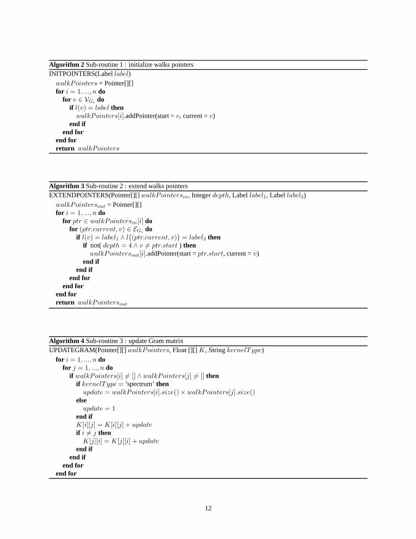
A pseudo code of the algorithm is given in Algorithms 1, 2, 3 and 4. Algorithm 1 is the main program in chargeof the tree-transveral process, and Algorithms 2, 3 and 4 aresubroutines, introduced to initialize the walks pointers,extend the pointed walks, and update the Gram matrix respectively. This pseudo-code relies on the abstract typesPointerandLabel, to represent the walk pointers involved in the algorithm, and the generic vertices and edges labels,belonging toLV andLN respectively. Formally, aPointer object consists of two graph vertices: astart andcurrentvertex, representing the first and the current vertices of the pointed walk being extended. To maintain walks pointerswithin each molecule, we introduce a matrix of pointerswalkPointers = Pointer[][] : this matrix is initially empty,and during the walk extension process,walkPointers[i][j] corresponds to thejth pointer of the molecular graphGi.The stopping criterion of the recursion is controled by an integer variabledepthcorresponding to the depth in the treeduring the transversal process. It is initialized to zero and incremented at each recursive call. Whendepthis three,a depth-three node was reached in the tree, which corresponds to pointers on length-two walks in the graphs. In thesubsequent recursive step,depthis four, and the pointers are updated to ensure that the extended walks correspondto self-returning ones. A leaf node is then reached and the recursion terminates, leading to an update of the Grammatrix. Note however that the recursion is aborted wheneverthe set of walk pointers becomes empty for all graphs,since we only need to reach the leaf nodes corresponding to the pharmacophores truly present in the set of graphs.
10

The Gram matrix is updated according to the spectrum (15), binary (16) or Tanimoto (17) definition of the kernel, andwe introduce an × n Gram matrixK, initialized to zero, together with a binary variablekernelTypethat can take thevalues ’spectrum’, ’binary’ or ’Tanimoto’.
Computing the Gram matrixK simply requires a call to theCOMPUTEfunction of Algorithm 1 with these initial-ized data :COMPUTE(walkPointers, depth, K, kernelType), for a specifiedkernelType, and where the Pointer arraywalkPointers is empty,depth equals zero and the Gram matrixK is filled with zeros. Note however that in the caseof the Tanimoto kernel type, this procedure computes the ’raw’ kernel that actually corresponds to the binary kernel(16). The matrixK must be further normalized according to defintion 5, that is :K[i][j] = K[i][j]
K[i][i]+K[j][j]−K[i][j] .
The cost of this algorithm depends on the number of leaf nodesvisited, and is therefore bounded by the totalnumber of leaves of the tree, that is(np)3 if the number of distinct vertex labels isn and the number of distance bins isp. However, the maximum number of distinct pharmacophores that can be found in the moleculem is |m|3, and we donot need to exhaustively transverse the tree. This means that to compute the kernel between the moleculesm andm′,at mostmin(|m|3, |m′|3) leaves, corresponding to the common pharmacophores ofm andm′, need to be visited. Thecomplexity of the algorithm is thereforeO
(
min(
(np)3, min(
|m|3, |m′|3)))
1. For small molecules, the cost of thekernel will therefore depend on their number of atoms, whileit will depend on the size of the discrete pharmacophoresspace for large molecules.
Note finally that although we omit the details, the previous algorithm and complexity analysis hold for the two-points versions of the kernels : the tree involved in the recursive transversal process is smaller (a depth-two tree, withn2p leaf nodes), and the complexity is reduced toO
(
min(
n2p, min(|m|2, |m′|2)))
.
Algorithm 1 main programCOMPUTE(Pointer[][]walkPointers,Integerdepth, Float[][] K, StringkernelT ype)
depth = depth + 1if depth = 1 then
for label ∈ LV dowalkPointers = initPointers(label)compute(walkPointers, depth)
end forelse
for label1 ∈ LV dofor label2 ∈ LE do
walkPointers = extendPointers(walkPointers, depth, label1, label2)if iwalkPointers 6= [][] then
if depth = 4 thenupdateGram(walkPointers, K, kernelT ype)
elsecompute(walkPointers, depth)
end ifend if
end forend for
end if
7 Experiments
We now turn to the experimental section. The problem considered here consists in building predictive models to distin-guishactivefrom inactivemolecules on several protein targets. This problem is naturally formulated as a supervisedbinary classification problem that can be solved by SVM.
1Note however that in the case of the Tanimoto kernel (17), theself kernels have to be computed, and the worst case complexity of the algorithmis O
(
min(
(np)3, |m|3 + |m′|3))
.
11
Algorithm 2 Sub-routine 1 : initialize walks pointersINITPOINTERS(Labellabel)
walkPointers = Pointer[][]for i = 1, ..., n do
for v ∈ VGido
if l(v) = label thenwalkPointers[i].addPointer(start =v, current =v)
end ifend for
end forreturn walkPointers
Algorithm 3 Sub-routine 2 : extend walks pointersEXTENDPOINTERS(Pointer[][]walkPointersin, Integerdepth, Labellabel1, Labellabel2)
walkPointersout = Pointer[][]for i = 1, ..., n do
for ptr ∈ walkPointersin[i] dofor (ptr.current, v) ∈ EGi
doif l(v) = label1 ∧ l
(
(ptr.current, v))
= label2 thenif not(depth = 4 ∧ v 6= ptr.start ) then
walkPointersout[i].addPointer(start =ptr.start, current =v)end if
end ifend for
end forend forreturn walkPointersout
Algorithm 4 Sub-routine 3 : update Gram matrixUPDATEGRAM(Pointer[][]walkPointers, Float [][] K, StringkernelT ype)
for i = 1, ..., n dofor j = 1, ..., n do
if walkPointers[i] 6= [] ∧ walkPointers[j] 6= [] thenif kernelT ype = ’spectrum’then
update = walkPointers[i].size()× walkPointers[j].size()else
update = 1end ifK[i][j] = K[i][j] + updateif i 6= j then
K[j][i] = K[j][i] + updateend if
end ifend for
end for
12

TRAIN TESTPos Neg Pos Neg
BZR 94 87 63 62COX 87 91 61 64DHFR 84 149 42 118ER 110 156 70 110
Table 1: Basic informations about the datasets considered.
7.1 Datasets
We tested the pharmacophore kernel on several datasets usedin a recent SAR study (32). More precisely, we consid-ered the following four publicly available datasets2:
• theBZRdataset, a set of 405 ligands for the benzodiazepine receptor,
• theCOXdataset, a set of 467 cyclooxygenase-2 inhibitors,
• theDHFRdataset, a set of 756 inhibitors of dihydrofolate reductase,
• theERdataset, a set of 1009 estrogen receptor ligands.
These datasets contain the 3D structures of the molecules, together with a quantitative measure of their ability toinhibit a biological mechanism. Datasets were filtered and split into training and test sets according to a particular datapreparation scheme detailed in (32). Table 1 gathers basic informations about the datasets involved in the study.
7.2 Experimental setup
We investigated in this study a simple labeling scheme to describe each atom (hydrogen atoms were systemati-cally removed), and therefore the potential pharmacophores: the label of an atom is composed of its type (e.g.,C, O, N ...) and the sign of its partial charge (+,− or 0). Hence the set of labels can be expanded asL ={
C+, C0, C−, O+, O0, O−, . . .}
. The partial charges account for the contribution of each atom to the total chargeof the molecule, and were computed with the QuacPAC softwaredeveloped by OpenEye3. It is important to note that,contrary to the physicochemical properties of atoms, partial charges depend on the molecule and describe the spatialdistribution of charges. Although the partial charges takecontinuous values, we simply kept their signs for the labelingas basic indicators of charges in the description of pharmacophores. We callcategorical kernelthe kernel resultingfrom this labeling, where the kernel between labelsKFeat is the Dirac kernel (10) and the kernel between distancesKDist is the Gaussian RBF kernel (9).
Alternatively, we tested several variants of this basic categorical kernel. First, we tested the effect of the partialcharges by removing them from the labels, and keeping the same Dirac and Gaussian RBF kernels for the labels anddistances, respectively. In this case the label of an atom reduces to its type. Second, we tested alternatives to the Dirackernel between labels, by taking into account similaritiesbetween physicochemical properties of atoms with differentlabels. We considered the four following properties, takenfrom (33) : theVan der Waals radius, which represents theradius of an imaginary sphere enclosing the atom, thecovalent radius, corresponding to half of the distance betweentwo identical covalently bonded atomic nuclei, thefirst ionization energy, the energy required to strip it of an electronfrom the atom, and theelectronegativity, a measure of the ability of an atom or molecule to attract electrons in thecontext of a chemical bond. The Van der Waals and covalent radii account for the steric property of atoms, while thetwo latter properties encode their electrostatic behavior. In these cases, for computational reasons, a triangular kernelwas used to compare different atoms with respect to these properties. Third, we tested the six fast approximationsmentioned in Section 6 with our original labeling scheme (3- and2-points spectrum, binary and Tanimoto kernels).
In addition, we tested the state-of-the-art Tanimoto kernel based on the 2D structure of molecules (19) to evaluatethe potential gain obtained by including 3D information. This kernel is defined as the Tanimoto coefficient betweenfingerprints indicating the presence or absence of all possible molecular fragments of length up to8 in the 2D structure
2Available as supporting information of the original study at http://pubs.acs.org/journals/jcisd8/3http://www.eyesopen.com/products/applications/quacpac.html
13
of the molecule, where a fragment refers to a sequence of atoms connected by covalent bonds. We note that thisfingerprint is similar to classical 2D-fingerprints such as the Daylight representation4, with the difference that ourimplementation does not require to fold the fingerprint intoa small-size vector (18).
The different kernels were implemented in C++, and the SVM experiment was conducted with the freely availablePython machine learning package PyML5. For each experiment, all parameters of the kernel and the SVM were op-timized over a grid of possible choices on the training set only, to maximize the mean area under the ROC curve(AUC) (34) over an internal 10-fold cross-validation. The results on the test set correspond to the performanceof the SVM with the selected parameters only. The optimized parameters include the widthσ ∈ {0.1, 1, 10} (inangstroms) of the Gaussian RBF kernel used to compare distances, the soft-margin parameter of the SVM over thegrid {0.1, 0.5, 1, 1.5, ..., 20}, the number of bins used to discretize the distances for the fast approximations over thegrid {4, 6, 8, . . . , 30} and the cut-off parameterC of the triangular kernel when physicochemical properties are used.This later parameter was chosen among3 values chosen such that10, 25 or 50% of all atom pairs in the training sethave a non-zero value for the kernel. The largerC, the more atoms of distinct types are matched by the kernel, but thelonger the kernel computation.
7.3 Results
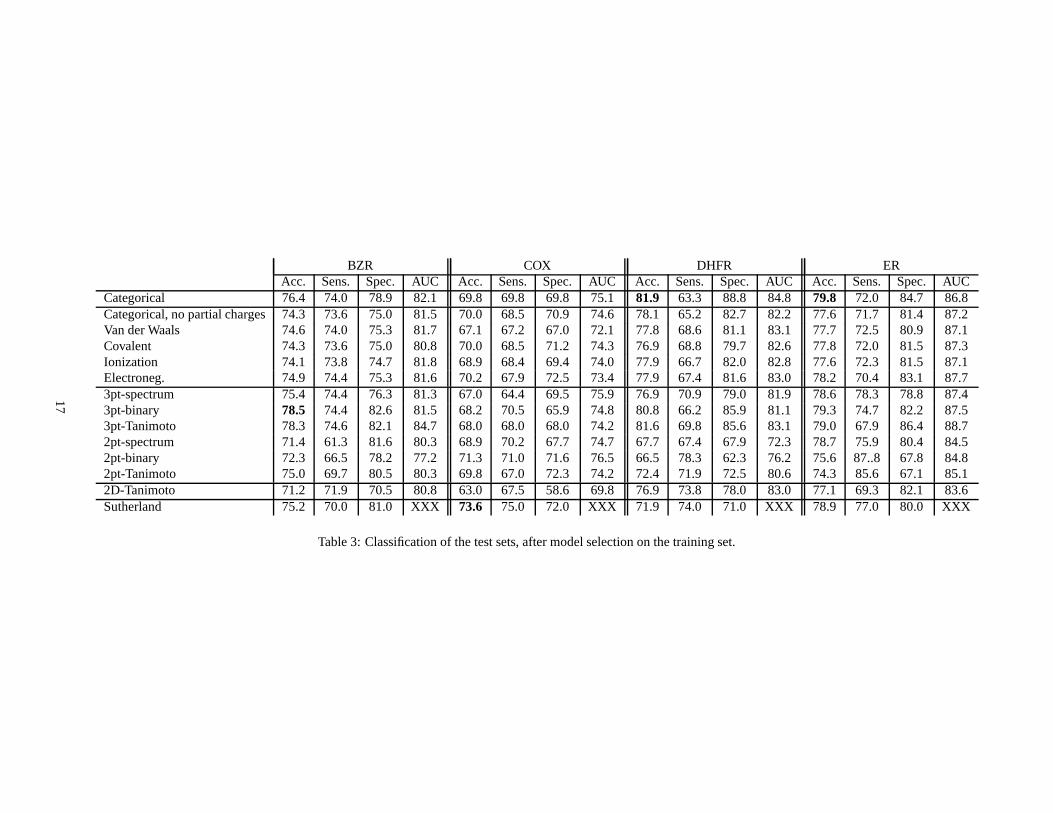
Table 3 shows the results of classification for the differentkernel variants. Each line corresponds to a kernel, andreports several statistics : the accuracy (fraction of correctly classified compounds), sensitivity (fraction of positivecompounds that were correctly classified), specificity (fraction of negative compounds that were correctly classified),and AUC. The first line corresponds to the basic categorical kernel. The following five lines show the results ofthe five variants of the categorical kernel obtained by modifying the kernel between labels (Dirac kernel for labelswithout partial charges, and triangular kernel for4 physicochemical properties). The results obtained by the six fastapproximations follow. Finally, we added the performance obtained by the state-of-the-art 2D Tanimoto kernel basedon the 2D structure of the molecules and the best results reported in the reference publication (32).
The results of parameters optimization on the training set often led to similar choices for different kernels. Forexample, the width of the Gaussian RBF kernel to compare distances was usually selected at0.1 angstrom, whichcorresponds to a very strong constraint on the pharmacophore matching. The cut-off parameter for the triangularkernel was usually chosen to allow10 or 25% of matches between atoms on the training set. Finally, the number ofbins selected by the fast approximations to discretize the distances was usually between 20 and 30 bins.
The results show that in general, the five variants of the categorical kernel obtained by modifying the kernelbetween labels (lines 2-6) lead to similar or slightly worseperformances than the categorical kernel. Removing thepartial charges from atom labels decreases the accuracy by3 to 5% on all datasets except COX, confirming thatthe partial charge information is important for the definition of pharmacophores. The variants based on the fourphysicochemical properties of atoms lead to results globally similar to those obtained with atom type labels withoutpartial charges, from which they are deduced. This shows that, in the context of this study, subtle pharmacophoricfeatures based on physicochemical parameters instead of simply the type of atoms could not be detected.
The fast pharmacophore kernel obtained by applying a Dirac kernel to check when pairs of candidate pharma-cophores fall in the same bin of the discretized space (3pt-spectrum) systematically degrades the accuracy of1 to 5%over all four datasets compared to the categorical kernel. This suggests that the gain in computation time obtained bydiscretizing the space and computing a 3D-fingerprint-likerepresentation of molecules has a cost in terms of accuracyof the final model. A particular limitation of the fingerprint-based method is that two pharmacophores could remainunmatched in they fall into two different bins, although they might be very similar but close to the bins boundaries. Inthe case of the pharmacophore kernel, such pairs of similar pharmacophores would always be matched.
Interestingly, however, performances competitive with the categorical kernel are obtained by the fast 3pt-binaryand 3pt-Tanimoto kernels. On the BZR dataset, the 3pt-binary kernel even gives the best performance. Contrary to the3pt-spectrum kernel, these kernels are not pharmacophore kernels in the sense of Definition 2; however they are basedon the same representation as the 3pt-spectrum kernel, the only difference being the way to obtain the kernel valuefrom the fingerprint description. Note finally that these twokernels give overall similar results.
We observe moreover that except for the COX dataset, the discrete kernels based on two-points pharmacophoreslead to significantly worse results than their three-pointscounterparts.
4http://www.daylight.com/dayhtml/doc/theory/theory.toc.html5Available athttp://pyml.sourceforge.net
14

Exact DiscreteWith charges 20’ 6’Without charges 249’ 7’
Table 2: Computation times in minutes needed to compute the different kernel matrices on the BZR training set. Thefirst column refers to the computation of the exact kernel (6), and the second one to the approximate kernels (15) and(17).
For each dataset, the results obtained with the 2D-Tanimotokernel are significantly worse than those of the cat-egorical kernel, with a decrease ranging from3 to 7% on the different datasets. This confirms the relevance of 3Dinformation for drug activity prediction, that motivated this work. Finally we note that on all but the COX dataset,the categorical kernel outperforms the best results of (32), confirming the competitiveness of our method compared tostate-of-the-art methods.
Regarding the computational complexity of the different methods, Table 2 shows the time required to compute thekernel matrices on the BZR training set for different kernels, on a desktop computer, equipped with a Pentium 4 - 3.6GHz processor, and 1 GB RAM. In the discrete version, the distance range was split into 24 bins, and as expected, thekernels based on the discretization of the pharmacophore space are faster than their counterparts by a factor of4 to 35,depending on the type of labels used (with or without the partial charge information). In the exact kernel computation,the effect of removing the partial charges from the labels isto induce more matches between atoms and therefore, asdiscussed in Section 4, to drastically slow the computationby a factor of12, consistent with the theoretical estimatethat dividing the size of the label classes byk increases the speed by a factork3.
8 Discussion and conclusion
This paper presents an attempt to extend the application of recent machine learning algorithms for classification tothe manipulation of 3D structures of molecules. This attempt is mainly motivated by applications in drug activityprediction, for which 3D pharmacophores are known to play important roles. Although previous attempts to definekernels for 3D structures (similar in fact to the 2pt-spectrum kernel we tested) led to mixed results (35), we obtainedperformance competitive with state-of-the-art algorithms for the categorical kernel based on the comparison of phar-macophores contained in the two molecules to be compared. This kernel is not an inner product between fingerprints,and therefore fully exploits the mathematical trick that allows SVM to manipulate measures of similarities rather thanexplicit vector representations of molecules, as opposed to other methods such as neural networks. We even observedthat for the closest fingerprint-based approximation obtained by discretizing the space of possible pharmacophores(3pt-spectrum kernel), the performance significantly decreases. This highlights the benefits that can be gained fromthe use of kernels, which provide a satisfactory answer to the common issue of choosing a “good” discretization ofthe pharmacophore space to make fingerprints: once discretized, pharmacophores falling on different sides of binsedges do not match although they might be very close. We notice that approaches based on fuzzy fingerprints (36), forexample, aim at correcting this effect by matching pharmacophores based on different distance bins.
Although the best overall method in this study is the categorical kernel, it is interesting to notice that very compet-itive results are obtained by the binary and Tanimoto kernels applied to the discretized pharmacophore representation.Compared to the 3pt-spectrum, the better performance of thebinary kernel suggests that the choice of the functionalform of the kernel given a representation of molecules can play a critical role in terms of performance. Representingpharmacophores by indicators (bits) of their presence rather than by their precise counts can be interpreted as a trivialway to emphasize rare versus frequent pharmacophores in thekernels. Alternatively, it might be possible for example,to adopt more flexible schemes to weight the pharmacophores depending on their probability of appearance in themolecules, and to modify in a similar way the functional formof the pharmacophore kernels (Definition 2) to improveperformance over the categorical kernel.
Concerning the practical use of our approach for screening of large datasets, Table 2 shows that, even for the fastestvariants, the approach based on kernel methods can be computationally demanding even for relatively small datasets.In practice, however, the time to train the SVM can be smallerthan the times presented in Table 2 because not allentries of the matrix are required. Speeding up SVM and kernel methods for large datasets is currently a topic ofinterest in the machine learning community, and applications in virtual screening on large databases of molecules will
15
certainly benefit from the advances in this field.Among the possible extensions to our work, a first direction would be to test and validate different definitions
and labeling for the vertices of the pharmacophores. We limited ourselves to the simplest possible3-points phar-macophores based on single atoms annotated by their types and partial charges. The method could be improved bytesting other schemes known to be relevant features as basiccomponents of pharmacophores. Instead of single atoms,it is for example possible to consider groups of atoms forming functional units instead of single atoms to form phar-macophores. A second possible extension is to generalize this work to pharmacophores with more points, e.g.,4 or5. Although several results will not remain valid in this case, such as the expression of the kernel as the trace of amatrix, this could lead to more accurate models in cases where the binding mechanism is well characterized by suchpharmacophores. Finally, a third promising direction thatis likely to be relevant for many real-world applications isto take into accounts different conformers of each molecule. Indeed, it is well-known that the biological activity to bepredicted is often due to one out of several conformers for a given molecule, which suggests to represent a moleculenot as a single 3D structure but as a set of structures. The kernel approach lends itself particularly well to this exten-sion, thanks to the possibility to define kernels between sets of structures from a kernel between structures, just likewe defined a kernel between sets of pharmacophores from a kernel between single pharmacophores.
References
[1] Charles Manly, Shirley Louise-May, and Jack Hammer. Theimpact of informatics and computational chemistryon synthesis and screening.Drug Discov. Today, 6(21):1101–1110, Nov 2001.
[2] Darko Butina, Matthew D Segall, and Katrina Frankcombe.Predicting ADME properties in silico: methods andmodels.Drug Discov. Today, 7(11 Suppl):S83–S88, Jun 2002.
[3] C. A. Lipinski, F. Lombardo, B. W. Dominy, and P. J. Feeney. Experimental and computational approaches toestimate solubility and permeability in drug discovery anddevelopment settings.Adv. Drug. Deliv. Rev, 46(1-3):3–26, Mar 2001.
[4] R. D. King, S. H. Muggleton, A. Srinivasan, and M. J. E. Sternberg. Structure-activity relationships derivedby machine learning: The use of atoms and their bond connectivities to predict mutagenicity by inductive logicprogramming.Proc. Natl. Acad. Sci. USA, 93:438–442, 1996.
[5] Hans-Joachim Bohm, Gisbert Schneider, Raimund Mannhold, Hugo Kubinyi, and Gerd Folkers.Protein-ligandinteractions. Wiley, 2003.
[6] Inbal Halperin, Buyong Ma, Haim Wolfson, and Ruth Nussinov. Principles of docking: An overview of searchalgorithms and a guide to scoring functions.Proteins, 47(4):409–443, Jun 2002.
[7] C. Lemmen and T. Lengauer. Computational methods for thestructural alignment of molecules.J. Comput.Aided. Mol. Des., 14(3):215–232, Mar 2000.
[8] L. Xue and J. Bajorath. Molecular descriptors in chemoinformatics, computational combinatorial chemistry, andvirtual screening.Comb. Chem. High. Throughput Screen., 3(5):363–372, Oct 2000.
[9] J. D. Holliday and P. Willett. Using a genetic algorithm to identify common structural features in sets of ligands.J. Mol. Graph. Model., 15(4):221–232, Aug 1997.
[10] Paul Finn, Stephen Muggleton, David Page, and Ashwin Srinivasan. Pharmacophore discovery using the induc-tive logic programming language Progol.Machine Learning, 30:241–270, 1998.
[11] Hans Matter and Thorsten Potter. Comparing 3D pharmacophore triplets and 2D fingerprints for selecting diversecompound subsets.J. Chem. Inf. Model., 39:1211–1225, 1999.
[12] R. D. Brown and Y. C. Martin. The information content of 2D and 3D structural descriptors relevant to ligand-receptor binding.J. Chem. Inf. Comput. Sci., 37:1–9, 1997.
[13] J. Bajorath. Selected concepts and investigations in compound classification, molecular descriptor analysis, andvirtual screening.J. Chem. Inf. Comput. Sci., 41(2):233–245, 2001.
16
BZR COX DHFR ERAcc. Sens. Spec. AUC Acc. Sens. Spec. AUC Acc. Sens. Spec. AUC Acc. Sens. Spec. AUC
Categorical 76.4 74.0 78.9 82.1 69.8 69.8 69.8 75.1 81.9 63.3 88.8 84.8 79.8 72.0 84.7 86.8Categorical, no partial charges74.3 73.6 75.0 81.5 70.0 68.5 70.9 74.6 78.1 65.2 82.7 82.2 77.6 71.7 81.4 87.2Van der Waals 74.6 74.0 75.3 81.7 67.1 67.2 67.0 72.1 77.8 68.6 81.1 83.1 77.7 72.5 80.9 87.1Covalent 74.3 73.6 75.0 80.8 70.0 68.5 71.2 74.3 76.9 68.8 79.7 82.6 77.8 72.0 81.5 87.3Ionization 74.1 73.8 74.7 81.8 68.9 68.4 69.4 74.0 77.9 66.7 82.0 82.8 77.6 72.3 81.5 87.1Electroneg. 74.9 74.4 75.3 81.6 70.2 67.9 72.5 73.4 77.9 67.4 81.6 83.0 78.2 70.4 83.1 87.73pt-spectrum 75.4 74.4 76.3 81.3 67.0 64.4 69.5 75.9 76.9 70.9 79.0 81.9 78.6 78.3 78.8 87.43pt-binary 78.5 74.4 82.6 81.5 68.2 70.5 65.9 74.8 80.8 66.2 85.9 81.1 79.3 74.7 82.2 87.53pt-Tanimoto 78.3 74.6 82.1 84.7 68.0 68.0 68.0 74.2 81.6 69.8 85.6 83.1 79.0 67.9 86.4 88.72pt-spectrum 71.4 61.3 81.6 80.3 68.9 70.2 67.7 74.7 67.7 67.4 67.9 72.3 78.7 75.9 80.4 84.52pt-binary 72.3 66.5 78.2 77.2 71.3 71.0 71.6 76.5 66.5 78.3 62.3 76.2 75.6 87..8 67.8 84.82pt-Tanimoto 75.0 69.7 80.5 80.3 69.8 67.0 72.3 74.2 72.4 71.9 72.5 80.6 74.3 85.6 67.1 85.12D-Tanimoto 71.2 71.9 70.5 80.8 63.0 67.5 58.6 69.8 76.9 73.8 78.0 83.0 77.1 69.3 82.1 83.6Sutherland 75.2 70.0 81.0 XXX 73.6 75.0 72.0 XXX 71.9 74.0 71.0 XXX 78.9 77.0 80.0 XXX
Table 3: Classification of the test sets, after model selection on the training set.
17
[14] B. E. Boser, I. M. Guyon, and V. N. Vapnik. A training algorithm for optimal margin classifiers. InProceedingsof the 5th annual ACM workshop on Computational Learning Theory, pages 144–152. ACM Press, 1992.
[15] V. N. Vapnik. Statistical Learning Theory. Wiley, New-York, 1998.
[16] R. Burbidge, M. Trotter, B. Buxton, and S. Holden. Drug design by machine learning: support vector machinesfor pharmaceutical data analysis.Comput. Chem., 26(1):4–15, December 2001.
[17] E. Byvatov, U. Fechner, J. Sadowski, and G. Schneider. Comparison of support vector machine and artificialneural network systems for drug/nondrug classification.J Chem Inf Comput Sci, 43(6):1882–9, 2003.
[18] P. Mahe, N. Ueda, T. Akutsu, J.-L. Perret, and J.-P. Vert. Graph kernels for molecular structure-activity relation-ship analysis with support vector machines.J. Chem. Inf. Model., 45(4):939–51, 2005.
[19] L. Ralaivola, S. J. Swamidass, H. Saigo, and P. Baldi. Graph kernels for chemical informatics.Neural Netw.,18(8):1093–1110, Sep 2005.
[20] B. Scholkopf and A. J. Smola.Learning with Kernels: Support Vector Machines, Regularization, Optimization,and Beyond. MIT Press, Cambridge, MA, 2002.
[21] H. Kashima, K. Tsuda, and A. Inokuchi. Kernels for graphs. In B. Scholkopf, K. Tsuda, and J.P. Vert, editors,Kernel Methods in Computational Biology, pages 155–170. MIT Press, 2004.
[22] C. J. C. Burges. A Tutorial on Support Vector Machines for Pattern Recognition.Data Min. Knowl. Discov.,2(2):121–167, 1998.
[23] J. Shawe-Taylor and N. Cristianini.Kernel Methods for Pattern Analysis. Cambridge University Press, 2004.
[24] M. A. Aizerman, E. M. Braverman, and L. I. Rozonoer. Theoretical foundations of the potential function methodin pattern recognition learning.Automation and Remote Control, 25:821–837, 1964.
[25] N. Aronszajn. Theory of reproducing kernels.Trans. Am. Math. Soc., 68:337 – 404, 1950.
[26] O. F. Guner.Pharmacophore Perception, Development, and Use in Drug Design, volume 2 ofIUL BiotechnologySeries. International University Line, 2000.
[27] D. Haussler. Convolution Kernels on Discrete Structures. Technical Report UCSC-CRL-99-10, UC Santa Cruz,1999.
[28] T. Gartner, P. Flach, and S. Wrobel. On graph kernels: hardness results and efficient alternatives. In B. Scholkopfand M. Warmuth, editors,Proc. of the Sixteenth Annual Conference on Computational Learning Theory and theSeventh Annual Workshop on Kernel Machines, volume 2777 ofLecture Notes in Computer Science, pages129–143, Heidelberg, 2003.
[29] S. D. Pickett, J. S. Mason, and I. M. McLay. Diversity profiling and design using 3D pharmacophores :pharmacophores-derived queries (PQD).J. Chem. Inf. Comput. Sci., 36:1214–1223, 1996.
[30] J. Saeh, P. Lyne, B. Takasaki, and D. Cosgrove. Lead hopping using SVM and 3D pharmacophore fingerprints.J. Chem. Inf. Model., 45(4):1122–1133, Jul 2005.
[31] C. Leslie, E. Eskin, and W.S. Noble. The spectrum kernel: a string kernel for SVM protein classification. InRuss B. Altman, A. Keith Dunker, Lawrence Hunter, Kevin Lauerdale, and Teri E. Klein, editors,Proceedingsof the Pacific Symposium on Biocomputing 2002, pages 564–575. World Scientific, 2002.
[32] J. J. Sutherland, L. A. O’Brien, and D. F. Weaver. Spline-fitting with a genetic algorithm : a method for develop-ing classification structure-activity relationships.J. Chem. Inf. Comput. Sci., 43:1906–1915, 2003.
[33] John Emsley.The Elements (third edition). Oxford University Press, 1998.
[34] T. Fawcett. ROC graphs: notes and practical considerations for data mining researchers. Technical Report2003-4, HP Laboratories, Palo Alto, CA, USA, 2003.
18

[35] S. J. Swamidass, J. Chen, J. Bruand, P. Phung, L. Ralaivola, and P. Baldi. Kernels for small molecules and theprediction of mutagenicity, toxicity and anti-cancer activity. Bioinformatics, 21(Suppl. 1):i359–i368, Jun 2005.
[36] Dragos Horvath and Catherine Jeandenans. Neighborhood behavior of in silico structural spaces with respectto in vitro activity spaces-a novel understanding of the molecular similarity principle in the context of multiplereceptor binding profiles.J. Chem. Inf. Comput. Sci., 43:680–690, 2003.
19