Embed Size (px)
Citation preview

PAUL R. KRUGMAN Massachusetts Institute of Technology
RICHARD E. BALDWIN Columbia University
The Persistence of the U.S.
Trade Def cit
THE FAILURE of the U.S. trade deficit to show marked improvement after two years of a falling dollar has become a major source of strain in the politics of economic policy. Frustrated with the persistence of the trade deficit, the administration has demanded reflation by unwilling German and Japanese governments. Congressional calls for protectionist mea- sures have become increasingly strident. Also at stake is the credibility of mainstream economists. Since signs of a deterioration in U.S. trade performance became clear-cut in 1982, most economists have argued that the fault lay in the strong dollar, not in other popular villains such as foreign countries' industrial policies. Further, the role of the dollar in causing the trade deficit is a key part of the widely accepted doctrine that links trade deficits to the federal budget deficit. If the trade deficit remains intractable, this doctrine, which has served as a potent defense against nationalistic views of the trade problem, will soon lose its effectiveness.
The purpose of this paper is to analyze the puzzling persistence of the trade deficit. We consider and reject several ideas that have recently become popular in explaining that persistence, and conclude that a valid explanation has three main parts. First is the accepted view that there
We would like to thank William L. Helkie, of the Federal Reserve Board of Governors, who provided much of our data and also gave invaluable assistance in discussion. Richard Haas, of the International Monetary Fund, also provided both crucial data and valuable discussion. Our thanks also to Peter Hooper and Catherine Mann at the Board and to Harry Foster and participants in seminars at the Board of Governors and the World Bank.
1
2 Brookings Papers on Economic Activity, 1:1987
are substantial lags in the adjustment of both prices and quantities to exchange rates, probably representing a tendency of firms to commit themselves to suppliers for extended periods of time. The effect of these lags has been heightened by the timing of the dollar's rise and fall: because the dollar rose steeply before it began falling, firms were still adjusting to the strength of the dollar and shifting to foreign suppliers even as the dollar fell. Second, the failure of foreign demand to grow as rapidly as U.S. demand since 1980 means that, other things equal, the dollar would have to fall below its 1980 level to restore the 1980 trade position. Finally, the evidence suggests that even if both the real exchange rate and relative demand were restored to their 1980 levels, the trade balance would still not return to its original position. At least in the years before 1980, there appears to have been a secular decline in the U.S. real exchange rate consistent with any given trade balance, but we have been unable to extract clear evidence of such a continuing trend from the data.
The paper is in six parts. The first part reviews some basic facts about U.S. trade performance, especially since the turnaround of the dollar in the first quarter of 1985. The second part addresses three widely circulated views about the reasons for a persistent trade deficit that can be confronted and rejected without formal econometric testing. The third part presents some "conventional econometrics" on U.S. trade, estimating a simple model of the nonagricultural, nonoil trade balance. The fourth part considers the issue of lags, presenting and testing some alternative views about the reasons for long lags in both prices and quantities. The fifth part addresses the possibility of a downward trend in the equilibrium exchange rate and asks whether the strong dollar itself shifted down the equilibrium exchange rate. The last part of the paper pulls the results together for an overall assessment.
Background on the Trade Deficit
As a preliminary to the discussion of the causes of the trade deficit's persistence, we review some basic facts about the U.S. trade position. These facts may be grouped under four subjects: exchange rate devel- opments, trade volumes, trade prices, and the trade balance itself.

Paul R. Krugman and Richard E. Baldwin 3
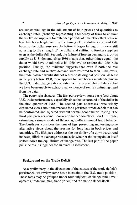
Figure 1. The Real Exchange Value of the U.S. Dollar, 1975:1-1987:1a
Natural logarithms
2.70
Real exchange rate
2.65 -
2.60 -
2.55 -
2.50 -
2.45
1976:1 1978:1 1980:1 1982:1 1984:1 1986:1
Source: Authors' calculations. Exchange rate and price data are from International Monetary Fund, International Financial Statistics, various issues. Manufacturing trade data are from U.S. Department of Commerce, International Trade Administration, United States Trade: Performance in 1985 and Outlook (Government Printing Office, 1986).
a. The real exchange rate expresses the ratio of the dollar price of U.S. goods to the dollar price of foreign goods and is here calculated as the quarterly average exchange rate for the U.S. dollar against the currencies of Japan, Canada, France, Germany, Italy, the United Kingdom, South Korea, and Taiwan, weighted by 1984 shares of U.S. manufacturing trade and deflated by wholesale prices of manufactures for industrial countries, and by overall wholesale prices for South Korea and Taiwan.
EXCHANGE RATES
Figure 1 presents a measure of the U.S. real exchange rate for manufactures. The index includes the currencies of six industrial coun- tries, plus Korea and Taiwan, weighted by 1984 bilateral manufactures trade with the United States. Prices are measured by wholesale prices

4 Brookings Papers on Economic Activity, 1:1987
for manufactures for the industrial countries, by wholesale prices overall for Korea and Taiwan.
The fall in the real dollar since its 1985: 1 peak has essentially reversed all of its rise from 1980. Some confusion has been created in popular discussion by exchange rate indexes that show little fall in the dollar. Figure 1 shows that the dollar has indeed fallen sharply, to levels no higher on average than those of the late 1970s. I
The overall fall in the dollar's real exchange rate, however, conceals disparities in its movements against currencies of different countries; in particular, the real dollar has fallen sharply against currencies of Western Europe and Japan, reaching a record low against the yen, while remaining relatively stable against currencies of both Canada and the newly industrializing countries (South Korea and Taiwan). These disparities raise a caution about speaking loosely about "the" exchange rate: a 1 percent decline in one exchange rate index may not mean at all the same thing as a 1 percent decline in another.
Another important feature of the exchange rate for understanding the persistence of the trade deficit may also be seen in figure 1: the dollar rose sharply just before it fell. The two-year decline in the dollar since the first quarter of 1985 followed a four-and-one-half-year rise, which was marked by a sharp run-up in the last three quarters. (Many observers regard this final run-up in the dollar as a speculative bubble, but that is outside the scope of this paper.) The fact that the fall came after a rise meant that U.S. trade flows had not fully adjusted to the strength of the dollar in early 1985, and lagged responses to the rising dollar before 1985:1 are crucial to understanding the peculiar dynamics since then.
It is also important to note that the strong dollar of the 1980s was actually not all that strong in the light of historical experience. The exchange rate peak in 1985, universally regarded as representing a severe overvaluation relative to the rate needed to achieve current account balance, in fact was by some measures about the same as the exchange rate of 1970, which appears to have been consistent with current account balance. This observation suggests a secular downward trend in the exchange rate consistent with any given U.S. external balance.
1. For some systematic comparisons of indexes with and without LDCs, see Martin Feldstein and Philippe Bochetta, "How Far Has the Dollar Really Fallen?" Working Paper 2122 (National Bureau of Economic Research, 1987).
Paul R. Krugman and Richard E. Baldwin 5
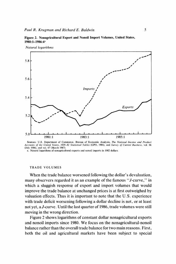
Figure 2. Nonagricultural Export and Nonoil Import Volumes, United States, 1980:1-1986:4a
Natural logarithms
5.8 -
5.6 -
Imports
5.4 0/ /
Exports
5.2 -- - V
5 0 I A h I A I I
1981:1 1983:1 1985:1
Sources: U.S. Department of Commerce, Bureau of Economic Analysis, The National Income antd Prodluct Accounts of the United States, 1929-82 Statistical Tables (GPO, 1986), and Survey of Cu4rrent Business, vol. 66 (July 1986), and vol. 67 (March 1987).
a. Natural logarithms of nonagricultural exports and nonoil imports in 1982 dollars.
TRADE VOLUMES
When the trade balance worsened following the dollar's devaluation, many observers regarded it as an example of the famous "J-curve," in which a sluggish response of export and import volumes that would improve the trade balance at unchanged prices is at first outweighed by valuation effects. Thus it is important to note that the U.S. experience with trade deficit worsening following a dollar decline is not, or at least not yet, aJ-curve. Until the last quarter of 1986, trade volumes were still moving in the wrong direction.
Figure 2 shows logarithms of constant dollar nonagricultural exports and nonoil imports since 1980. We focus on the nonagricultural-nonoil balance rather than the overall trade balance for two main reasons. First, both the oil and agricultural markets have been subject to special

6 Brookings Papers on Economic Activity, 1:1987
developments that would require extended analysis that would make the paper unwieldy. If those markets were the key to the persistence of the deficit, the detour would be unavoidable, but in fact the puzzle of deteriorating trade performance is perfectly clear in the nonagricultural- nonoil numbers as well as in the total. Second, much of the discussion of U.S. competitive problems has focused on manufacturing, and we would like to focus on a measure that mostly reflects manufacturing trade; while it would in principle be better to focus on manufacturing alone, the nonagricultural-nonoil data are both more carefully con- structed and more up-to-date than manufacturing price and volume data.
The figure makes two points. First, import volume not only continued to rise after the dollar's peak, it continued to rise about as rapidly as it had in the year before the peak, at about a 10 percent annual rate. Given U.S. GNP growth at only a 3 percent annual rate over the same period, the continuing rapid rise in import volume is fairly startling.
Second, while export volume rose in the year following the dollar's turnaround, it continued to rise more slowly than import volume; furthermore, it actually rose less rapidly in the seven quarters between 1985:1 and 1986:4 than it did in the year before the dollar's peak.
Any explanation of the persistence of the U.S. trade deficit must explain why trade volumes were still moving the wrong way for at least a year and a half after the dollar began to fall.
TRADE PRICES
The puzzle of perverse trade volumes may be linked to a second puzzle, that of pricing on the import side. Figure 3 shows an index of U.S. nonoil import prices deflated by U.S. manufactures wholesale prices and an index of the real import exchange rate, using foreign CPIs and the GNP deflator. What is immediately obvious is that until late 1986 there was essentially no discernible effect of the exchange rate on import prices. Foreign producers must have been taking large cuts in profit margins rather than raise the dollar prices of their goods in the United States. The practice is most apparent for Japan, where manufacturing unit labor costs in dollars rose 5.7 percent from 1985:1 to 1986:4 even while manufactures export prices fell 23.4 percent.
The picture on the export side has been different. If U.S. producers were, like foreign producers, to react to an exchange rate change by "pricingto market" -holding prices stable in the purchaser's currency-

Paul R. Krugman and Richard E. Baldwin 7
Figure 3. The Real Import Exchange Rate and Real Nonoil Import Prices, United States, 1980:1-1986:4
Index, 1980:1 =0
0.3_
0.2 Real import exchange ratea
0.1
0.0
-0.1I
-0.2 Real import pricesb
-0.3 __
-0.41.. l l .. 1981:1 1983:1 1985:1
Source: Authors' calculations with data from Survey of Current Business, various issues, and from IMF, International Financial Statistics, various issues.
a. Exchange value of the dollar deflated by relative import prices, calculated here as the ratio of the dollar price of U.S. goods (GNP deflator) to the dollar price of foreign goods (consumer prices).
b. U.S. nonoil import prices deflated by U.S. manufactures wholesale prices.
U.S. export prices in dollars would have surged since early 1985. In fact they have remained stable in dollar terms. Apparently U.S. producers have by and large not taken advantage of the dollar's fall to increase profit margins.
THE TRADE DEFICIT
There are two useful measures of the overall nonagricultural-nonoil trade deficit. The first is the actual or nominal deficit; the second is the "real" deficit, defined as exports minus imports measured in 1982 dollars. The real deficit represents an index of the combined effects of changes in export and import volumes, leaving aside price changes; the difference between the real and nominal deficits can be taken as a measure of terms- of-trade effects.
8 Brookings Papers on Economic Activity, 1:1987
From the dollar's peak in 1985: 1 to 1986:4 the nominal nonagricultural- nonoil deficit rose from $81 billion to $150 billion, while the real deficit rose from $93 billion to $136 billion. This joint rise reflects the fact that the United States has not, or at least not yet, experienced a J-curve, in which sluggish adjustment of the real trade deficit is offset at first by a worsening of the terms of trade. The real deficit has moved the wrong way, while, because of the asymmetrical behavior of import and export prices, there has been little change in the terms of trade.
Common Beliefs about the Trade Deficit
The failure of the trade deficit to fall despite the dollar's decline has led to wide circulation of explanations that either deny the actuality of dollar decline or dismiss it as irrelevant. The three most influential are that the dollar has not really fallen against a broad basket of currencies; that resolution of the trade deficit depends not on the dollar but on foreign economic growth, which has been insufficient; and that trade balances reflect differences between income and spending, and exchange rates are irrelevant. All three explanations have considerable appeal and touch upon valid points. However, each can be rejected as the central explanation of the puzzle.
HAS THE DOLLAR REALLY FALLEN?
Considerable press attention was given in 1986 to the publication by the Federal Reserve Bank of Dallas of an exchange rate index that included 131 countries, rather than the limited group of industrial countries covered by most widely circulated indexes.2 According to the Dallas index, the dollar had hardly declined at all from its early 1985 peak, a finding that was widely cited as a key explanation of the failure of the trade balance to improve.
The reason for the dollar's strong showing in the Dallas index was that while it had depreciated sharply against the currencies of Japan and Western Europe, the currencies of many less developed countries had actually depreciated against the dollar. In particular, if countries were
2. W. Michael Cox, "A New Alternative Trade-Weighted Dollar Exchange Rate Index," Economic Review of the Federal Reserve Bank of Dallas (September 1986), pp. 20-28.

Paul R. Krugman and Richard E. Baldwin 9
weighted by their trade with the United States, the continuing deprecia- tion of the currencies of Mexico, Brazil, and Argentina largely out- weighed the rise of the yen and European currencies.
It was immediately obvious to international economists, however, if not to the news media, that the sharp depreciation of high-inflation currencies did not explain the persistence of the U.S. trade deficit. Cost competitiveness depends on the real exchange rate, not the nominal rate, and the huge nominal depreciations of Latin American currencies had not been matched by corresponding real depreciations. A real exchange rate index shows a large dollar decline even with LDCs in the index. The index shown in figure 1, in fact, includes the most important LDC exporters of manufactures, South Korea and Taiwan, with a significant weight. Nonetheless, it shows a sharp dollar depreciation that has essentially reversed the 1980-85 rise.
THE ROLE OF FOREIGN GROWTH
The need for foreign growth to create demand for U.S. exports has been a central theme of U. S. official pronouncements on the trade deficit. Both Paul Volcker and James Baker have placed strong emphasis on the need for faster growth in Europe and Japan, and at times the Treasury has used the threat of a falling dollar as a goad to Germany and Japan to reflate their economies. Other authorities have emphasized the impor- tance of demand from LDCs, placing weight on the link between the debt problem and the trade deficit.
One might expect that an issue given such prominence in policy debate must necessarily be of major importance. Yet while it is true that faster growth abroad would help resolve the U.S. trade deficit, and while divergence between U.S. and foreign demand growth contributed sig- nificantly to the emergence of the U.S. trade deficit, the possible extent to which foreign demand growth could be expected to reduce the trade deficit, and thus the extent to which limited foreign demand can be assigned a key role in the persistence of the U.S. deficit, is almost certainly quite limited.
We will document this point with econometric evidence later, but the argument can be made with a simple back-of-the-envelope calculation. Indeed, for those who distrust econometrics, such a calculation may be more persuasive than the more careful documentation. In the fourth quarter of 1986, in nominal terms, U.S. imports of nonpetroleum
10 Brookings Papers on Economic Activity, 1:1987
products exceeded U.S. exports of nonagricultural goods by 74 percent. (In the late 1970s, by contrast, nonagricultural exports consistently exceeded nonoil imports.) Suppose that all foreign countries were somehow persuaded to expand their domestic demand 5 percent relative to what it would otherwise have been. Since imports from the United States are only a small fraction of the rest of world income, such an expansion in demand without a dollar depreciation would fall primarily on foreign goods, leading to an increase of foreign output of at least 4 percent-which for most countries exceeds the maximum that they believe can be achieved without creating dangerous inflationary pres- sure.3 Suppose also that the elasticity of U.S. exports with respect to foreign real expenditure is 3, which is well above most estimates (our preferred estimate is 2.1 -see below). Then this unlikely large reflation would increase U.S. exports 15 percent, only 20 percent of the increase needed to restore balance in nonagricultural-nonoil trade. Any plausible increase in foreign growth would contribute substantially less. Thus the lack of stronger foreign economic growth, while not totally irrelevant, is a secondary factor in explaining the persistence of the trade deficit.
Given the numbers, one may wonder why the growth issue receives so much attention. One answer may be simple misunderstanding, as in the case of the confusion over the extent of the dollar's fall. A more charitable explanation is that the emphasis on foreign growth represents shrewd politics on the part of U.S. economic officials. Blaming inade- quate foreign demand is a last line of defense against protectionists who deny the efficacy of the exchange rate in correcting trade imbalances. Furthermore, the emphasis on foreign demand, and the assertion that the dollar must fall unless such demand is provided, has accomplished a remarkable public relations feat: Secretary Baker may be the first finance minister in history to make currency devaluation seem a sign of strength, not weakness.
THE RELEVANCE OF THE EXCHANGE RATE
Recently an important challenge to the conventional analysis of exchange rates has been mounted by monetarist advocates of fixed
3. The International Monetary Fund estimates a GNP gap that is less than 4 percent for all of the Group of Seven countries and much less for several. See IMF, World Economic Outlook (IMF, April 1987).

Paul R. Krugman and Richard E. Baldwin 11
exchange rates, notably Robert Mundell and Ronald McKinnon.4 Their argument is that the exchange rate is irrelevant to trade balance deter- mination. Instead, the trade balance is determined by the difference between national income and national expenditure, or, equivalently, by the difference between saving and investment.
The Mundell-McKinnon view goes beyond asserting that the equality between the trade balance and the savings-investment balance is an identity. It carries a positive implication: that the trade balance has nothing to do with the exchange rate and that therefore the puzzle of a falling dollar and a rising deficit is no puzzle at all. The view also carries a normative implication: since exchange rates are irrelevant to trade balance adjustment, they should be fixed in order to achieve other aims, notably price stability.
Since their view has gained considerable influence in policy circles, it is important to consider it carefully. In fact, the Mundell-McKinnon view is logically wrong in its dismissal of any puzzle in the exchange rate-trade link and is almost surely empirically wrong in its policy message. To see why, it is helpful to have a rudimentary model in which the consequences of assumptions can be fully worked out.
A Simple Model. In a world economy consisting of two countries, the United States and the rest of the world (ROW), each country is assumed to produce a single good that is both consumed domestically and exported. We let ROW's output be numeraire and define p as the relative price of the U.S. good.
In Mundell's and McKinnon's discussions there is an implicit as- sumption of full employment and constant output. The assumption is not realistic, but to do away with it would create the impression that this is another Keynesian-classical dispute, which it is not. So let us assume that the United States produces a fixed output y and ROW produces a fixed output y*.
The determination of demand is another issue that is important but not central to understanding the exchange rate-trade balance linkage. Let us therefore treat total U.S. expenditure, measured in terms of the
4. Robert A. Mundell, "A New Deal on Exchange Rates," paper presented at Japan- United States Symposium on Exchange Rates and Macroeconomics (Tokyo, Japan, January 29-30, 1987); and Ronald I. McKinnon and Kenichi Ohno, "Getting the Exchange Rate Right: Insular versus Open Economies," paper presented at the meeting of the American Economic Association, December 1986.

12 Brookings Papers on Economic Activity, 1:1987
U.S. good, as a parameter, a. For the world as a whole income must equal expenditure. Thus if a* is ROW expenditure, measured in terms of the ROW good, it must be true that
(1) pa + a* =py +y*,or
a* = y* + p(y - a).
Now it is certainly true as an accounting identity that the trade balance is equal to the excess of income over expenditure, so that the U.S. trade balance, t, in terms of the U.S. good, is simply
(2) t = y - a,
an expression in which the relative price of U.S. goods does not directly appear.
The absence of that term does not, however, allow us to forget about relative prices. There is still a requirement that the market for U.S. output clear, in which case the market for ROW output clears as well, by Walras's Law. Each country will divide its expenditure between the two goods. For simplicity, let us make the Cobb-Douglas assumption that expenditure shares are fixed, with the United States spending a share m of its income on imports and 1 - m on domestic output, and ROW spending m* on imports and 1 - m* on domestic goods. Then we can write the market-clearing condition as
(3) py = (1 - m)pa + m*a*, or
p[y -(1- m)a] = m*a* = m*[y* + p(y - a)],
implying
(4) p = m*a*/D, where
D = (1 - m)y - (1 - m - m*)a.
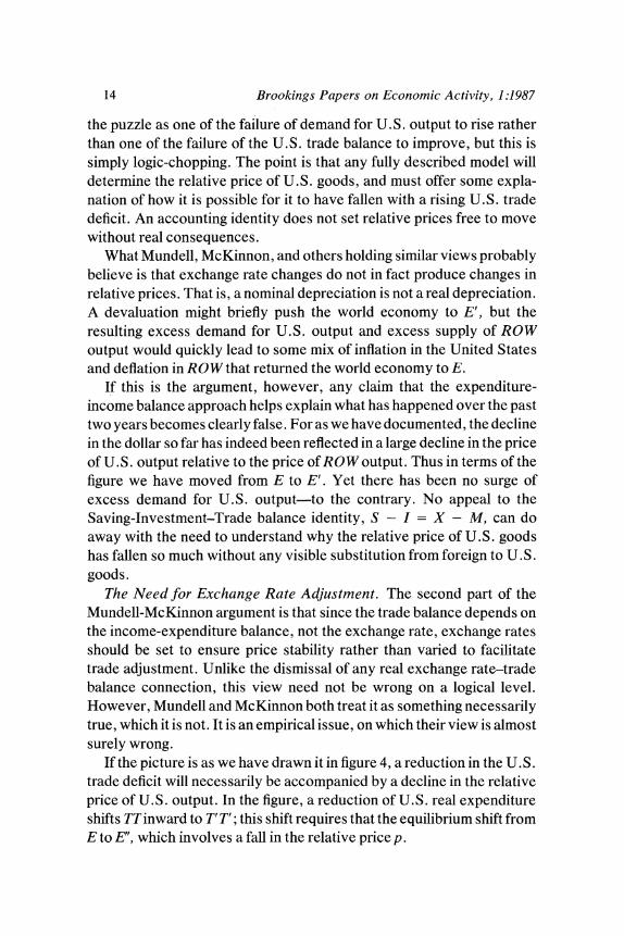
The implications of this small model are illustrated in figure 4, which is much more general than the example. On the horizontal axis is the U.S. level of real expenditure a; on the vertical axis is the relative price of U.S. output p. The line TT is an iso-trade-balance line, that is, it represents a locus of points consistent with some given trade balance in terms of U.S. output. The accounting identity that equates the trade balance to income minus expenditure, regardless of relative prices, is reflected by the fact that TTis vertical. Meanwhile, the line UUrepresents points of market clearing for U.S. output. It is here drawn with a positive

Paul R. Krugman and Richard E. Baldwin 13
Figure 4. Relative Price Adjustment
Relative price of U.S. output
T' T
U
/ElE
T' T
I
U.S. real expenditure
slope, which will be the case if (1 - m) > m*, that is, if U.S. residents have a higher marginal propensity to spend on U.S. output than ROW residents do. Point E is the equilibrium for a given trade balance.
Is There a Puzzle? The first part of the Mundell-McKinnon argument, to repeat, is that one should not be surprised by the failure of devaluation to improve the U.S. trade position. Devaluation is irrelevant, because the trade balance is determined by the income-expenditure balance. That is, at a point like E' in figure 4 the relative price of U. S . output has fallen, but U.S. expenditure has not, so there will not be a reduction in the trade deficit.
It should be immediately clear what is wrong with this argument: it fails to look at the whole story. If we observe what looks like a move from E to E', we should be puzzled, because E' is not an equilibrium: it is aposition of excess demand for U.S. goods. If we like, we can describe
14 Brookings Papers on Economic Activity, 1:1987
the puzzle as one of the failure of demand for U.S. output to rise rather than one of the failure of the U.S. trade balance to improve, but this is simply logic-chopping. The point is that any fully described model will determine the relative price of U.S. goods, and must offer some expla- nation of how it is possible for it to have fallen with a rising U.S. trade deficit. An accounting identity does not set relative prices free to move without real consequences.
What Mundell, McKinnon, and others holding similar views probably believe is that exchange rate changes do not in fact produce changes in relative prices. That is, a nominal depreciation is not a real depreciation. A devaluation might briefly push the world economy to E', but the resulting excess demand for U.S. output and excess supply of ROW output would quickly lead to some mix of inflation in the United States and deflation in ROW that returned the world economy to E.
If this is the argument, however, any claim that the expenditure- income balance approach helps explain what has happened over the past two years becomes clearly false. For as we have documented, the decline in the dollar so far has indeed been reflected in a large decline in the price of U.S. output relative to the price of ROW output. Thus in terms of the figure we have moved from E to E'. Yet there has been no surge of excess demand for U.S. output-to the contrary. No appeal to the Saving-Investment-Trade balance identity, S - I = X - M, can do away with the need to understand why the relative price of U.S. goods has fallen so much without any visible substitution from foreign to U.S. goods.
The Need for Exchange Rate Adjustment. The second part of the Mundell-McKinnon argument is that since the trade balance depends on the income-expenditure balance, not the exchange rate, exchange rates should be set to ensure price stability rather than varied to facilitate trade adjustment. Unlike the dismissal of any real exchange rate-trade balance connection, this view need not be wrong on a logical level. However, Mundell and McKinnon both treat it as something necessarily true, which it is not. It is an empirical issue, on which their view is almost surely wrong.
If the picture is as we have drawn it in figure 4, a reduction in the U.S. trade deficit will necessarily be accompanied by a decline in the relative price of U.S. output. In the figure, a reduction of U.S. real expenditure shifts TTinward to T' T'; this shift requires that the equilibrium shift from E to E", which involves a fall in the relative price p.

Paul R. Krugman and Richard E. Baldwin 15
Figure 5. Expenditures, Substitution Effects, and Relative Price Adjustment
Relative price of U.S. output
T
U U
T
U.S. real expenditure
Now there are two circumstances in which this relative price adjust- ment need not take place. The first, the case in which U.S. and ROW goods are perfect substitutes, can surely be dismissed pretty much out of hand, on the basis of casual observation, on the basis of the huge relative price movements of the 1980s, and on the basis of econometric evidence like that presented later that indicates, if anything, that substi- tution effects in trade are surprisingly small. The other is the case in which spending patterns are identical between the countries, so that (1 - m) = m*. In either case, the effect is to make UU horizontal (figure 5), so that a reduction in U.S. expenditure need not be accompanied by a decline in the relative price of what the United States produces.

16 Brookings Papers on Economic Activity, 1:1987
The case of identical spending patterns is famous in international economics as Bertil Ohlin's position on the transfer problem. It relies on the view that as expenditure falls in the United States and rises abroad, foreign residents will spend as much of their incremental income on U.S. goods as the reduction in U.S. spending on these goods. After decades of analysis of this point, it is also clear why this will not happen in practice. Briefly, because most output is not traded, residents of each country will spend relatively more of their income on local goods, both on average and at the margin. If U.S. expenditure were to fall $150 billion, while expenditure in the rest of the world rose the same amount, U.S. residents would cut their demand for U.S. goods something like $125 billion while foreigners would raise their spending on U.S. output no more than $25 billion. A fall in the relative price of U.S. goods would be necessary to close the resulting $100 billion excess supply.
The relative price changes that trade adjustment requires need not come through exchange rate adjustment. They could come instead through inflation in the country that increases its spending or deflation in the other country. One wonders whether even an economist who believed in flexible prices would regard either of these alternatives as the desirable route. In any case, price inertia gives a strong reason for preferring to adjust the exchange rate.
The Conventional Econometrics of the Trade Balance
In this section we set out some basic, "conventional" econometric analysis of the U.S. nonagricultural-nonoil trade balance. By conven- tional we mean that it follows the approaches taken by standard fore- casting equations. Real expenditures and prices of goods other than those of U.S. imports and exports are taken as exogenous. Lags are estimated on an ad hoc basis, unconstrained by any formal dynamic model. The experience with volatile exchange rates since 1970 has in important respects been a vindication for such conventional modeling. With plenty of variation in the data even the simplest estimation techniques yield plausible results, and the simple equations have by and large successfully tracked the impact of the exchange rate on the trade balance.

Paul R. Krugman and Richard E. Baldwin 17
Table 1. Determinants of Nonagricultural Export Volume, Selected Periods, 1977:2-1986:4a
Independent variable Elasticity and summary statistic 1977:2-1985:1 1977:2-1986:4
Foreign real expenditure 2.47 (0.18) 2.42 (0.13) Real exchange rate (sum of lags) - 1.40 (0.13) - 1.33 (0.11)
Lags: 0 - 0.29 (0.09) - 0.23 (0.05) 1 -0.25 (0.05) -0.21 (0.03) 2 -0.21 (0.03) -0.19 (0.02) 3 -0.18 (0.02) -0.17 (0.01) 4 -0.14 (0.03) -0.15 (0.02) 5 - 0.11 (0.04) -0.12 (0.02) 6 -0.09 (0.04) -0.10 (0.02) 7 - 0.06 (0.04) - 0.08 (0.02) 8 -0.04 (0.03) -0.05 (0.02) 9 - 0.02 (0.02) - 0.03 (0.01)
Summary statistic R2 0.904 0.916 Standard error 0.032 0.033 Durbin-Watson 0.77 0.72
Source: Authors' calculations with foreign real expenditure data supplied by the Board of Governors of the Federal Reserve; exchange rate and price data from the International Monetary Fund and from IMF, International Financial Statistics, various issues; and manufacturing trade data used in the exchange rate calculations from U.S. Department of Commerce, International Trade Administration, United States Trade: Performance in 1985 and Outlook (Government Printing Office, 1986).
a. Quarterly data. Dependent variable is U.S. nonagricultural export volume (in 1982 prices). Independent variables are defined as follows. Foreign real expenditure is GDP plus imports minus exports in 1982 prices for eighteen countries weighted by U.S. export shares; the real exchange rate expresses the ratio of the dollar price of U.S. goods to the dollar price of foreign goods and is here calculated as the average exchange rate of the U.S. dollar against the currencies of Japan, Canada, France, Germany, Italy, the United Kingdom, South Korea, and Taiwan, weighted by 1984 shares of U.S. manufacturing trade and deflated by wholesale prices of manufactures for industrial countries and by overall wholesale prices for South Korea and Taiwan. Elasticities here and elsewhere measure the effect on the dependent variable of a 1 percent change in the independent variable. Numbers in parentheses are standard errors.
TRADE VOLUMES
Tables 1 and 2 present simple equations for U.S. nonagricultural export and nonoil import volume. The explanatory variables are real domestic expenditure in the importing market (defined as GDP plus imports minus exports in 1982 prices) and a distributed lag on the real exchange rate.
Many estimated trade equations use GNP rather than expenditure because the data are more readily available. On grounds of theoretical clarity, expenditure is preferable; in practice, the results are not much affected by the choice.

18 Brookings Papers on Economic Activity, 1:1987
Table 2. Determinants of Nonoil Import Volume, Selected Periods, 1977:2-1986:4a
Independent variable Elasticity and summary statistic 1977:2-1985:1 1977:2-1986.4
U.S. real expenditure 2.78 (0.12) 2.87 (0.12) Real exchange rate (sum of lags) 0.92 (0.13) 0.86 (0.14)
Lags: 0 0.14 (0.05) 0.03 (0.04) 1 0.14 (0.03) 0.07 (0.02) 2 0.13 (0.02) 0.09 (0.02) 3 0.12 (0.02) 0.11 (0.02) 4 0.11 (0.02) 0.12 (0.02) 5 0.09 (0.03) 0.12 (0.02) 6 0.08 (0.03) 0.11 (0.03) 7 0.06 (0.03) 0.10 (0.02) 8 0.04 (0.02) 0.07 (0.18) 9 0.02 (0.01) 0.04 (0.01)
Summary statistic R2 0.98 0.99 Standard error 0.025 0.028 Durbin-Watson 1.71 1.34
Source: Authors' calculations with U.S. expenditure data from U.S. Department of Commerce, Bureau of Economic Analysis, The National Income and Product Accounts of the United States, 1929-82 Statistical Tables (GPO, 1986), and Survey of Current Business, various issues; exchange rate and price data from the IMF and from Intertiational Finatncial Statistics, various issues; and manufacturing trade data used in the exchange rate calculations from International Trade Administration, United States Trade.
a. Quarterly data. Dependent variable is U.S. nonoil imports (in 1982 prices). Independent variables are defined as follows. U.S. real expenditure is GNP plus imports minus exports in 1982 prices; the real exchange rate expresses the ratio of the dollar price of U.S. goods to the dollar price of foreign goods. It is calculated as described in table 1. Numbers in parentheses are standard errors.
The equations are estimated both from 1977:2 to 1985: 1, the dollar's peak, and from 1977:2 to the end of 1986. The estimates are not much affected by the recent bad news about U. S. trade performance. However, if the estimates over the shorter time period are used to forecast forward, they do predict a U. S. trade recovery that has not yet happened. Export volume in 1986:4 was 5 percent less, and import volume 7 percent greater, than these equations predict; the real trade deficit was therefore $43 billion larger than we would have predicted.
One possibility is that there is a secular trend due to technological change that is not captured in these equations; we discuss the theoretical rationale for such a trend below. To test for the trend, we have also estimated the equations with a trend term and, for good measure, with time squared, to allow for a shifting trend. At first sight, the results,

Paul R. Krugman and Richard E. Baldwin 19
Table 3. Alternative Trade Volume Equations, 1977:2-1986:4
Independent Elasticity variable and Exports Imports Exports Imports
summary statistic (1) (2) (3) (4)
Real expenditurea 5.54 3.08 2.56 2.80 (0.64) (0.25) (1.35) (0.37)
Real exchange rateb 0.23 0.98 -2.77 0.54 (0.34) (0.13) (1.26) (0.44)
Timec -0.024 -0.0028 - 0.036 -0.011 (0.005) (0.002) (0.007) (0.008)
Time squared ... ... 0.0008 0.0002 (0.0003) (0.0002)
Summary statistic R2 0.95 0.99 0.96 0.99 Standard error 0.025 0.017 0.014 0.016 Durbin-Watson 1.18 1.94 1.46 1.88
Source: Authors' calculations with data as described in tables 1 and 2. Numbers in parentheses are standard errors.
a. For the export equations, the variable is foreign real expenditure, as described in table 1. For the import equations, the variable is U.S. real expenditure, as described in table 2.
b. Expresses the ratio of the dollar price of U.S. goods to the dollar price of foreign goods. It is calculated as in table 1 and equals the sum of a ten-quarter distributed lag.
c. Equals 1.0 for 1985:1.
reported in table 3, suggest much less confidence in the simple equations. Both price and especially income elasticities shift around considerably; in particular, if the estimate of a foreign demand elasticity of 5.5 were taken seriously, it would considerably modify our conclusion that foreign reflation can have only a modest impact on the trade deficit. However, we suspect that the trend terms are overexplaining the data, allowing random shocks and errors in variables to distort the results. An indication is that these equations do much worse than the simpler equations at forecasting out of sample. For example, the equations with a simple trend underpredict 1986:4 export volume by 11 percent and import volume by 15 percent; the equations with time and time squared overpredict export volume by 23 percent (although getting import volume within 2 percent). Thus while additional terms are significant in the estimation, we suspect that the simplest equations are to be preferred.
An important implication of these results is that while price elasticities in trade are clearly significant, and well outside the Marshall-Lerner condition that the sum of the price elasticities on exports and imports
20 Brookings Papers on Economic Activity, 1:1987
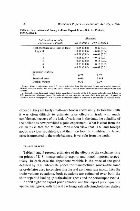
Table 4. Determinants of Nonagricultural Export Prices, Selected Periods, 1976:2-1986:4a
Independent variable Elasticity and summary statistic 1976:2-1985:1 1976:2-1986:4
Real exchange rate (sum of lags) - 0.35 (0.04) - 0.47 (0.04) Lags: 0 -0.11 (0.05) -0.08 (0.04)
1 -0.09 (0.02) -0.04 (0.02) 2 -0.06 (0.01) -0.12 (0.01) 3 -0.04 (0.03) -0.15 (0.02) 4 -0.03 (0.03) - 0.15 (0.02) 5 -0.01 (0.02) -0.09 (Q.01)
Summary statistic W2 0.72 0.77 Standard error 0.014 0.018 Durbin-Watson 0.51 0.39
Source: Authors' calculations with U.S. export price data from Thle Natiotnal Incomze atnd Product Accountts, 1929-82 Statistical Tables, and Survey of Cuirrent Business, various issues; manufactures wholesale prices are from the IMF.
a. Quarterly data. Dependent variable is the logarithm of the ratio of the U.S. nonagricultural export deflator to U.S. manufactures wholesale prices. The real exchange rate expresses the ratio of the dollar price of U.S. goods to the dollar price of foreign goods. It is calculated as described in table 1. Numbers in parentheses are standard errors.
exceed 1, they are fairly small-not too far above unity. Before the 1980s it was often difficult to estimate price effects in trade with much confidence, because of the lack of variation in the data; the volatility of the dollar has now provided a good experiment. What is clear from the estimates is that the Mundell-McKinnon view that U.S. and foreign goods are close substitutes, and that therefore the equilibrium relative price is unrelated to the trade balance, is very far from the truth.
TRADE PRICES
Tables 4 and 5 present estimates of the effects of the exchange rate on prices of U.S. nonagricultural exports and nonoil imports, respec- tively. In each case the dependent variable is the price of the good deflated by U.S. wholesale prices for manufactured goods-the same price deflator used in constructing the real exchange rate index. Like the trade volume equations, both equations are estimated over both the shorter period leading up to the dollar's peak and the period up to 1986:4.
At first sight the export price equation and the import price equation appear analogous, with the real exchange rate affecting both the relative

Paul R. Krugman and Richard E. Baldwin 21
Table 5. Determinants of Nonoil Import Prices, Selected Periods, 1976:2-1986:4a
Independent variable Elasticity and summary statistic 1976:2-1985:1 1976:2-1986:4
Real exchange rate (sum of lags) -0.98 (0.05) - 1.07 (0.05) Lags: 0 -0.52 (0.06) -0.27 (0.05)
1 - 0.31 (0.02) - 0.24 (0.02) 2 -0.15 (0.01) -0.21 (0.01) 3 - 0.04 (0.03) - 0.17 (0.02) 4 0.02 (0.03) -0.12 (0.02) 5 0.03 (0.02) -0.06 (0.02)
Summary statistic Rj2 0.95 0.93 Standard error 0.016 0.018 Durbin-Watson 0.52 0.26
Source: Same as table 4. a. Quarterly data. Dependent variable is the logarithm of the ratio of the U.S. nonoil import deflator to U.S.
manufactures wholesale prices. The real exchange rate expresses the ratio of the dollar price of U.S. goods to the dollar prnce of foreign goods. It is calculated as described in table 1. Numbers in parentheses are standard errors.
import and export prices with a substantial lag. However, the setup actually embodies a major asymmetry in the timing of import and export price responses. On the import side, a decline in the dollar is reflected only gradually in a rise in dollar import prices, and thus reflected only gradually in a rise in the relative price of foreign goods. On the export side, a decline in the dollar is at first met with no change in the dollar price of U.S. exports, and thus with an immediate fall in the price of U.S. goods relative to foreign goods. Only over time is there some upward adjustment in U.S. goods prices.
This asymmetry between export and import pricing reflects observed price behavior, as the contrast between the United States and Japan makes clear. Japanese export prices in yen have fallen sharply; in effect. the Japanese have chosen to cut into profit margins first, think about raising dollar prices later. By contrast, U. S. export prices in dollars have remained flat; that is, U.S. firms do not seem to hold their prices stable in foreign currency.
The reason for the asymmetry probably lies both in the size of the United States and in the special role of the dollar in international markets. As we will argue later, lags in the effect of exchange rates on both prices and quantities in international trade are best explained as consequences of commitments-implicit contracts-between buyers and suppliers.

22 Brookings Papers on Economic Activity, 1:1987
Pricing behavior in these implicit contracts presumably reflects the same considerations that affect more formal invoicing decisions, in which the choice of invoice currency reflects three broad rules. First, other things equal, invoice in the exporter's currency; second, other things equal, invoice in the currency of the larger trading partner; third, use dollars where both parties are small countries. Since the United States is both large and the key currency country, the bulk of U.S. trade is invoiced in dollars on both the import and export side. It appears that the same is true for the implicit contracts that govern trade pricing.5
The important point to note is that in the long run the exchange rate has plausible effects on prices; a dollar depreciation raises import prices roughly one-for-one while depressing export prices. In the short run there are significant lags in the effect of the exchange rate on prices. These lags help explain why the decline of the dollar has not yet been seen in a corresponding rise in import prices, especially since the dollar rose before it fell, and it has taken time for the effects of that rise to appear. However, both equations develop some forecasting problems when extrapolated out of sample; export prices are overestimated 9 percent, and import prices 9.5 percent.
THE SOURCES OF THE TRADE DEFICIT
The estimates in tables 1, 2, 4, and 5 allow us to do an accounting exercise, asking what the proximate causes of the trade deficit were. Table 6 performs the exercise by asking the following questions: how much of the trade deficit would have been avoided if each of the proximate causes had been absent? First, we ask how much the 1986:4 deficit would have been reduced if U.S. and foreign domestic demand had grown at the same rate; then we ask how much smaller it would have been if the real exchange rate had remained at its 1980:1 level; finally, we ask what would have happened if both the divergence in demand growth and the real appreciation had been avoided.
Effect of Differential Demand Growth. It is widely believed that a major cause of the trade deficit is that the United States has grown much more rapidly than the rest of the world in the 1980s. Somewhat surpris-
5. See Paul Krugman, "The International Role of the Dollar: Theory and Prospect," in John F. 0. Bilson and Richard C. Marston, eds., Exchange Rate Theory and Practice (University of Chicago Press, 1985), pp. 261-78.
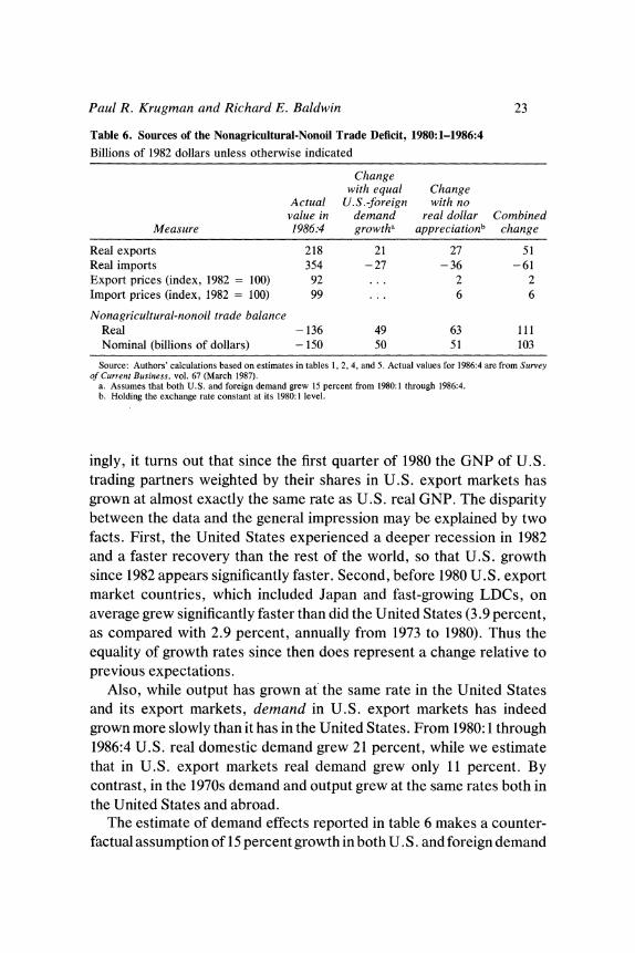
Paul R. Krugman and Richard E. Baldwin 23
Table 6. Sources of the Nonagricultural-Nonoil Trade Deficit, 1980:1-1986:4 Billions of 1982 dollars unless otherwise indicated
Change with equal Change
Actual U.S.-foreign with no value in demand real dollar Combined
Measure 1986:4 growtha appreciationb change
Real exports 218 21 27 51 Real imports 354 - 27 - 36 - 61 Export prices (index, 1982 = 100) 92 . . . 2 2 Import prices (index, 1982 = 100) 99 ... 6 6
Nonagricultural-nonoil trade balance Real - 136 49 63 111 Nominal (billions of dollars) - 150 50 51 103
Source: Authors' calculations based on estimates in tables 1, 2, 4, and 5. Actual values for 1986:4 are from Suirvey of Current Business, vol. 67 (March 1987).
a. Assumes that both U.S. and foreign demand grew 15 percent from 1980:1 through 1986:4. b. Holding the exchange rate constant at its 1980:1 level.
ingly, it turns out that since the first quarter of 1980 the GNP of U.S. trading partners weighted by their shares in U.S. export markets has grown at almost exactly the same rate as U.S. real GNP. The disparity between the data and the general impression may be explained by two facts. First, the United States experienced a deeper recession in 1982 and a faster recovery than the rest of the world, so that U.S. growth since 1982 appears significantly faster. Second, before 1980 U.S. export market countries, which included Japan and fast-growing LDCs, on average grew significantly faster than did the United States (3.9 percent, as compared with 2.9 percent, annually from 1973 to 1980). Thus the equality of growth rates since then does represent a change relative to previous expectations.
Also, while output has grown at the same rate in the United States and its export markets, demand in U.S. export markets has indeed grown more slowly than it has in the United States. From 1980:1 through 1986:4 U.S. real domestic demand grew 21 percent, while we estimate that in U.S. export markets real demand grew only 11 percent. By contrast, in the 1970s demand and output grew at the same rates both in the United States and abroad.
The estimate of demand effects reported in table 6 makes a counter- factual assumption of 15 percent growth in both U. S. and foreign demand

24 Brookings Papers on Economic Activity, 1:1987
from 1980:1 through 1986:4. Given the other factors pushing the U.S. real trade balance into deficit, such equal growth rates in demand would have implied significantly faster growth in the rest of the world than in the United States, as in the 1970s. It is questionable whether such an expectation was reasonable given the economic difficulties of Europe and the slowing of Japanese economic growth. Thus in our view this estimate of the effect of demand in causing the trade deficit is rather high. Nonetheless, it is clear that the divergence in demand growth has been a significant factor. On this estimate U. S. exports would have been about 10 percent higher, U.S. imports about 8 percent lower, with both the nominal and real trade deficits lower by about one-third.
The Exchange Rate. The next column of table 6 reports what would have happened if the U.S. real exchange rate had remained at its level in the first quarter of 1980. Even though the dollar's rise during the 1980s had been all but reversed by the end of 1986, lagged effects of the rise were still in evidence, and a constant 1980:1 real exchange rate would have had large effects on the volumes of exports and imports. According to the estimates, import volume would have been 10 percent less, while export volume would have been 12 percent greater. Thus about 45 percent of the real trade deficit would not have occurred.
The effects on the nominal trade balance are a bit smaller because depreciation raises import prices more than it raises export prices and thus creates a valuation effect that runs counter to the effect on volumes. About a third of the nominal deficit would have been avoided if the dollar had failed to appreciate.
The Residual. The results presented above suggest that the exchange rate and lower foreign demand growth do not explain all of the U.S. trade deficit. Had real dollar exchange rates remained at their 1980 level and had demand grown at the same rate in the United States and its export markets, an important part of the trade deficit would still be with us. The last column of the table shows that the combined effect of equal demand growth and no real appreciation would undo only 80 percent of the real trade deficit and two-thirds of the nominal trade deficit. This residual is comparable in importance to the two basic determinants that we have included in the estimation and is crucial to the puzzle of the persistence of the trade deficit at this point.
There are three plausible hypotheses that might explain why the trade deficit appears to be more persistent than demand and relative prices
Paul R. Krugman and Richard E. Baldwin 25
would warrant. First is that the lags in the adjustment of trade to the exchange rate are simply longer than our estimates suggest-so that the fact that the trade deficit continued to rise for two years after the dollar began falling represented the continuing cumulative effects of the dollar's previous rise. Second is that the well-publicized "competitiveness" problems of U.S. industry, notably lagging productivity growth and diminishing technological edge, require a secular downward trend in the real dollar exchange rate, so that the falling dollar has been chasing a moving target. A slight trend is in effect present in our estimates because the estimated expenditure elasticity of import demand exceeds that of export demand, but exponents of this hypothesis would argue that the effect is larger than this. Third is the possibility that the strong dollar did persistent damage to the U.S. trade position, the hypothesis of "hyster- esis" in the trade balance. In the remainder of this paper we consider each of these hypotheses in turn.
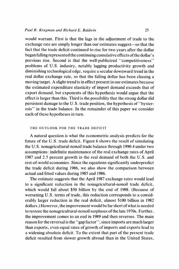
THE OUTLOOK FOR THE TRADE DEFICIT
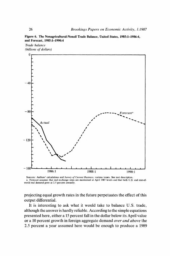
A natural question is what the econometric analysis predicts for the future of the U.S. trade deficit. Figure 6 shows the result of simulating the U.S. nonagricultural-nonoil trade balance through 1990:4 under two assumptions: indefinite maintenance of the real exchange rates of April 1987 and 2.5 percent growth in the real demand of both the U.S. and rest-of-world economies. Since the equations significantly underpredict the trade deficit during 1986, we also show the comparison between actual and fitted values during 1985 and 1986.
The estimate suggests that the April 1987 exchange rates would lead to a significant reduction in the nonagricultural-nonoil trade deficit, which would fall about $50 billion by the end of 1988. (Because of worsening U.S. terms of trade, this reduction corresponds to a consid- erably larger reduction in the real deficit, almost $100 billion in 1982 dollars.) However, the improvement would be far short of what is needed to restore the nonagricultural-nonoil surpluses of the late 1970s. Further, the improvement comes to an end in 1989 and then reverses. The main reason for the reversal is the "gap factor"; since imports are much larger than exports, even equal rates of growth of imports and exports lead to a widening absolute deficit. To the extent that part of the present trade deficit resulted from slower growth abroad than in the United States,
26 Brookings Papers on Economic Activity, 1:1987
Figure 6. The Nonagricultural-Nonoil Trade Balance, United States, 1985:1-1986:4, and Forecast, 1985:1-1990:4
Trade balance (billions of dollars)
0
-40 _
-80 ,- do- - F . Forecasta
Actual
%~~~~~~~~~~
- 120 -
-160 L I . . . A 1986:1 1988:1 1990:1
Sources: Authors' calculations and Survey of Current Business, various issues. See text description. a. Forecast assumes that real exchange rates are maintained at April 1987 levels and that both U.S. and rest-of-
world real demand grow at 2.5 percent annually.
projecting equal growth rates in the future perpetuates the effect of this output differential.
It is interesting to ask what it would take to balance U.S. trade, although the answer is hardly reliable. According to the simple equations presented here, either a 15 percent fall in the dollar below its April value or a 10 percent growth in foreign aggregate demand over and above the 2.5 percent a year assumed here would be enough to produce a 1989
Paul R. Krugman and Richard E. Baldwin 27
balance in nonagricultural-nonoil trade. One should bear in mind, however, that the equations are underpredicting the current trade deficit, so these projections may be underestimates of the adjustment needed.
This is about as far as one wants to push the conventional economet- rics. The next step is to ask what kind of microeconomic foundations might underly the key features of lags and a secular downward trend.
Behind the Econometrics: Lags
In our version of conventional econometrics, as in all standard models of the trade balance, a key element is the presence of long lags in the adjustment of both prices and volumes to the exchange rate. But although the lags are central to explaining the puzzle of a worsening trade balance in both real and nominal terms after early 1985, they are entirely ad hoc. Can a plausible microeconomic justification for the lags be offered?
We begin by considering the simplest view, that lags represent short- run supply inelasticity due to limits on the rate at which physical trade flows can be changed. They might, for example, represent order-delivery lags or bottlenecks in distribution. If the lags take this form, however, we ought to find income effects on trade prices and lags in the effect of income on trade volumes. We are unable, however, to find evidence of any such effects.
We then develop an alternative view, which emphasizes long-term commitments by importers to suppliers and accounts for the fact that income affects trade volumes much more rapidly than does the exchange rate.
SLOW ADJUSTMENT OF QUANTITIES
The simplest explanation of lags in the effect of exchange rates on both prices and volumes might be that the physical trade flows cannot be rapidly adjusted, or that it is costly to adjust them rapidly. This would have the effect of making the short-run supply curve for imports upward- sloping and would lead to slow adjustment of both prices and volumes to an exchange rate change.6
6. The analysis that follows draws on Catherine L. Mann, "Prices, Profit Margins, and Exchange Rates," Federal Reserve Bulletin, vol. 72 (June 1986), pp. 366-79.

28 Brookings Papers on Economic Activity, 1:1987
Figure 7. Market for U.S. Imports
Price
s Is~ ~ s
?~~~~~~~~~~~~~~~~~~~~~~~~~~~~~~~ IL
I\
. ~~~~~~~~~~~~~~~~~~~~~I
Quantity
Figure 7 makes the point. It shows a hypothetical market for a U.S. imported good. D is the demand curve; Ss is the short-run import supply curve, while SL is the long-run supply curve. The steeper slope of Ss reflects difficulties associated with adjusting the volume of imports quickly, such as long order-delivery lags and the need to establish new distribution networks. In the long run we show supply as perfectly elastic, reflecting the fact that even U.S. imports are generally a small fraction of world production of any given good. That is, the upward slope of the supply curve reflects the inelasticity of short-run supply to the United States rather than that to the world at large.
A dollar devaluation will shift both Ss and SL UP, so that in the long run the price will rise by the full amount of the devaluation. However, initially the inelasticity of supply will lead to only partial pass-through

Paul R. Krugman and Richard E. Baldwin 29
Figure 8. Effects of Demand on U.S. Import Volume
Price
ss
SL
Quantity
of the exchange rate into import prices. The initial rise in import prices will be only from E1 to E2. Over time there will then be further adjustment as the supply adjusts, leading to gradually rising import price and falling import volume, as indicated by the arrowheads, until E3 is reached.
So far so good. However, this interpretation has two other implica- tions: that domestic demand in the importing country should affect its import prices and that the effect of demand on import volume should also involve a lag comparable to the lag on the exchange rate. Figure 8 illustrates the point. If real expenditure in the importing country rises, D will shift outward. The initial effect will be a rise in the price of imports, as the equilibrium shifts from E1 to E; import prices will then fall as the supply curve shifts out and equilibrium moves to E3. Meanwhile, import volume will rise only part of its long-run amount initially, then rise for some time after the rise in real demand.

30 Brookings Papers on Economic Activity, 1:1987
Table 7. Tests for Short-Run Import Supply Inelasticity, 1977:2-1986:4a
Elasticity
Independent variable Import volume and summary statistic (1) (2) Import price
U.S. real expenditure 1.75 1.77 - 0.25 (0.46) (0.41) (0.04)
Lagged 1.03 0.77 ... (0.41) (0.31)
Two lags ... 0.19 ... (0.32)
Three lags .. . 0.04 ... (0.34)
Real exchange rateb 1.00 1.03 -0.84 (0.14) (0.14) (0.05)
Summary statistic Standard error 0.026 0.026 0.014 Durbin-Watson 1.32 1.31 0.45 R2 0.99 0.99 0.97
Source: Authors' calculations. See text and tables 1-5. a. Quarterly data. Dependent variables are U.S. nonoil imports (in 1982 prices) and import prices, which are
calculated as the logarithm of the ratio of the U.S. nonoil import deflator to U.S. manufactures wholesale prices. Numbers in parentheses are standard errors.
b. The real exchange rate expresses the ratio of the dollar price of U.S. goods to the dollar price of foreign goods. It is calculated as described in table 1. For the import volume equations, the real exchange rate is estimated as a ten-quarter distributed lag; for the import price equation, the variable is estimated with six lags.
This gives us two testable propositions: effects of aggregate demand on prices and lags in the effect of demand on volumes. Table 7 reports some tests of these propositions.
The results on prices do not support the idea that import supply is inelastic in the short run. There does not appear to be any significant effect of U.S. aggregate demand on import prices. Admittedly, trade prices as measured are often set in implicit or explicit long-term contracts and may not reflect the shadow price of imports that is relevant to demand. However, the results on quantities are also unsupportive. We find no evidence of lags in the effect of real expenditure on imports reaching beyond one quarter.
As usual, we should accept econometric results only if they seem to make sense given a broader view of the way things seem to work. What the results seem to say is a proposition embodied in most econometric trade models: namely, that income effects work much more quickly than price effects. Is this reasonable? Experience suggests that it is. For example, the slump in 1982 was immediately reflected in a decline in real nonoil imports despite the rising dollar; nonoil import volume fell 7

Paul R. Krugman and Richard E. Baldwin 31
percent from 1981:4 through 1982:4. As soon as the U.S. recovery began, import volume began rising; from 1982:4 through 1983:4 nonoil import volume rose 37.7 percent. Thus demand effects seem to work through very quickly. On the other hand, the experience of the last two years is as strong evidence as one could hope to have of long lags in the response of trade flows to the exchange rate. Thus we need a model that allows for a disparity in the rate of adjustment of trade flows to income and prices.
IMPLICIT CONTRACTS
An interpretation of trade that allows quick income effects but slow price effects is the following: importers make fairly long-term commit- ments about whom to buy from, but not about how much they will buy. We have come to think of this as the Book-of-the-Month-Club model. A subscriber to the Book-of-the-Month Club commits herself to buy only a minimum, above which her purchases may vary quite sharply from quarter to quarter. However, she will not arbitrage on a continual basis between BOMC and Quality Paperback Books; decisions about the club to which to belong will come relatively seldom.
There is anecdotal evidence that the same sort of behavior takes place in international trade. Executives of U. S. firms to whom we have spoken report that they make fairly long-term commitments to particular sup- pliers and that they are continuing to fulfill their commitment to use some foreign suppliers even though at this point U.S. suppliers would be cheaper. Since the commitment is to the particular supplier, but not to the volume of purchases, import volume may shift rapidly in response to changes in desired sales. But the composition of demand between domestic goods and imports will shift only slowly.
This description seems to lend itself naturally to a Taylor-style overlapping contract formulation, as shown in the following simple model. Imports and domestic products compete for consumers; for simplicity, we take the total volume demand of consumers as being totally inelastic with respect to prices. Thus let Q be the total volume demand for both imports and import-competing domestic production; we assume
(5) Qt= Q(At),
where At is real domestic expenditure.

32 Brookings Papers on Economic Activity, 1:1987
This total demand in turn is divided among domestic and foreign goods. We assume that each purchaser must decide once every n periods whether to commit to a domestic or foreign supplier. In each period the fraction of purchasers who choose imports will depend on the expected average price over the next n periods:
(6) t f(t)
The natural next assumption is that there is a distribution of pur- chasers, with a fraction lln making the decision each period. The result will be that the volume of imports, Mt, depends on GNP, Y, and on a flat distributed lag on expected prices:
(7) Mt= Q(Yt)[>f(Ptl1),
or, linearizing in the logs,
ln(Mt) = bo + b1ln(Yt) + b2 [ ln(P )j.
What determines prices? Since there is an implicit contract between buyer and supplier, a variety of pricing behaviors might be possible. One plausible candidate is that prices are kept fixed in the buyer's currency; another is that they are kept fixed in the seller's currency. In the first case, the price will be set in advance and will be proportional to the expected exchange rate; in the second, the price will be unknown, but the expected price will be proportional to the expected exchange rate. Thus in either case, we will have
(8) ln(Pe)
= k + ln(Ee).
Finally, we need to specify exchange rate expectations. Suppose that these expectations take a simple regressive form. That is, the expected exchange rate over the length of a commitment is a weighted average of the actual exchange rate at the beginning of the commitment and a ''normal" exchange rate E:
(9) ln(Ete) = aln(Et) + (1 - a)ln(E).
If a = 1 we have the case of static expectations.

Paul R. Krugman and Richard E. Baldwin 33
Then the import volume equation will take the form
(10) ln(Mt) = bo + bjAt + b2a> n(E, -)I.
This formulation, in which real demand enters on a current basis, while the exchange rate enters only as a distributed lag, is capable of explaining fast income but slow exchange rate effects.
The trade price equation will depend on who bears the exchange risk. If the price is set in supplier currency, the import price will respond immediately to the actual exchange rate:
(lla) ln(Pt) = k + ln(Et).
If the price is set in buyer's currency, it will have the same overlapping contract structure as the volume:
(llb) ln(Pt) = k + (1/n) a E ln(Et-1)i
If some mix of the two pricing schemes is present, it can be captured with the compromise equation:
n-
(lIc) ln(Pt) = k + wln(Et) + (1 - w) E ln(Et11 i=O
Now equation 1 Ic is very similar to the actual equations we have estimated, except for the constraint of a "horizontal" lag structure, which is itself the result of the arbitrary assumption that commitment lengths are the same for all importers, and we do not wish to impose the constraint in practice. Instead, equation 1 Ic should be seen as an illustration of how lag structures like those estimated in standard equations can be justified.
EXPLAINING SLOW TRADE RESPONSE
We can now explain the slowness of response of trade flows to the falling dollar. Taking first differences of equation 10, we have
(12) ln(Mt) - ln(M, -1) = bl[ln(At) - ln(At-1)] + b2a[ln(Et) -ln(Et- A

34 Brookings Papers on Economic Activity, 1:1987
The change in GNP that affects import volume is from last quarter; the change in the exchange rate is from n quarters ago because buyers currently choosing a supplier are just coming off commitments made some time ago.
The potential role of lags in explaining the apparent paradox of a declining dollar and a rising real trade deficit can now be seen. Because the dollar rose before falling, it was not until late 1985 that exchange rates were lower than they were two years previously. Thus buyers getting free of their commitments in 1985 may still have been switching to foreign suppliers, even though the dollar had fallen from its peak, because they made commitments to domestic suppliers when the dollar was still relatively low. If we imagine that commitments extend even more than two years, it is possible to argue that this lagged response extended some time into 1986.
If this is the right interpretation of lags in the effect of exchange rates, however, a turnaround should surely have come during 1986. By the second quarter of 1986 the exchange rate was at levels not seen since 1981; while there may have been a few long-term commitments to U.S. suppliers coming to an end and being replaced with commitments to foreign firms, surely most firms considering new commitments were already facing more favorable prices from U.S. suppliers than the last time they made such a choice. Thus the U.S. trade balance should have started to improve, at least in real terms, during 1986; indeed, the conventional econometric estimates reported earlier in this paper, when estimated up to the dollar's peak and projected forward, do indeed predict considerable improvement beginning in the second quarter of 1986. Since that improvement did not take place, we need to turn to other possible explanations of the trade deficit's persistence.
Does the Dollar Need to Decline Secularly?
There is a widespread belief that in order to restore equilibrium in the U.S. trade balance, the dollar must not only decline now but continue to decline in the future. This view arises from three kinds of evidence: the fact that the roughly balanced current account that the United States maintained through the 1970s was achieved only through an exchange rate that declined substantially from the beginning of the decade to its

Paul R. Krugman and Richard E. Baldwin 35
end; econometric estimates that have normally shown an income elas- ticity of demand for U. S. exports that is far less than the income elasticity of import demand; and the sense that the decline in U.S. technological and productivity leadership requires an offsetting decline in relative U.S. labor costs.
The exchange rate evidence is clear-cut for the decade of the 1970s. For example, the International Monetary Fund calculates five indicators of U.S. competitiveness in manufacturing, using as price deflators unit labor costs, value-added deflators, wholesale prices, and export unit values.7 All five measures declined from 1970 to 1980, although the size of the decline varies from 37 percent for relative unit labor costs to only 13 percent for relative export unit values. For relative unit labor costs and relative value-added deflators the average real exchange rates at the dollar's peak were only roughly comparable to the rates of the late 1960s. Since the United States kept its current account position relatively level over this period, the implication is that the dollar consistent with a given trade balance was declining secularly.
The econometric evidence comes primarily from the comparison of export and import income elasticities of demand. Until recently nearly all studies found that the income elasticity of demand for U.S. imports was considerably higher than the income elasticity of export demand; this implied that in order for imports and exports to grow at the same rate it was necessary to have continuing dollar depreciation.8 This disparity in income elasticities could simply be an accidental result of the mixes of goods that the United States and other countries produce, but it seems unlikely; many have concluded that the underlying cause has something to do with the catch-up of the rest of the world to the United States in capacity and technology. The widely used Federal Reserve model of the trade balance includes a "relative capacity" term designed to capture these factors; when that term was included, the income elasticities became more nearly equal, but the downward trend
7. IMF, International Financial Statistics, 1984 Yearbook (IMF, 1984). 8. The classic reference on income elasticities in world trade, which first pointed out
the apparent need for secular decline in the dollar (and the pound sterling) is H. S. Houthakker and Steven P. Magee, "Income and Price Elasticities in World Trade," Review of Economics and Statistics, vol. 51 (May 1969), pp. 111-25. The massive subsequent literature is surveyed in Morris Goldstein and Mohsin S. Khan, "Income and Price Effects in Foreign Trade," in Ronald W. Jones and Peter B. Kenen, eds., Handbook of International Economics, vol. 2 (Amsterdam: North-Holland, 1985), pp. 1041-1105.

36 Brookings Papers on Economic Activity, 1:1987
Table 8. Comparative Productivity Levels in Manufacturing, 1973 and 1984
Index, United States = 100
United United Year States Canada Japan France Germany Italy Kingdom
1973 100 89 56 62 78 67 57 1984 100 86 93 81 90 84 59
Source: Adapted from Molly McUsic, "U.S. Manufacturing: Any Cause for Alarm?" Newv Eniglanid Econiomic Review (Jan.-Feb. 1987), table 9.
was reintroduced by the fact that capacity grew more rapidly in the rest of the world than in the United States.9
Our econometrics, using more recent data and somewhat different variables from most other studies, shows only a small difference between export and import income elasticities. This by itself would seem to suggest that the need for secular dollar decline, although present in the 1970s, may have faded away in the 1980s, as other countries converged on the United States. On the other hand, we have seen that a substantial part of the current deficit remains unexplained by our estimated price and income effects. Skepticism about the ability of econometrics to separate the effects of the strong dollar from any possible secular decline leads us to ask whether there is other evidence bearing on the issue.
This brings us to the third kind of evidence for the hypothesis of secular decline: the diminishing U.S. productivity and technological advantage over competing nations. The widespread concern over U.S. competitiveness reflects not only the trade deficit, but also the fact that U.S. productivity is being overtaken by other countries (table 8). In addition to what has happened to measured productivity, there is a sense that the United States has lost its edge in the introduction of new products. Businessmen and some economists tend to assume that this loss of productivity-technological edge requires a decline in the real exchange rate over time. However, the conclusion is not as clear-cut as one might suppose.
9. This point was first made by Peter Hooper, "The Stability of Income and Price Elasticities in U.S. Trade, 1957-1977," International Finance Discussion Paper 119 (Board of Governors of the Federal Reserve System, June 1978). Hooper introduced a "relative supply" variable measuring the ratio of U.S. and rest-of-world capital stocks. The presence of this variable accounts for the equality of import and export income elasticities found in William L. Helkie and Peter Hooper, "The U.S. External Deficit in the 1980s," in Ralph C. Bryant and others, eds., Empirical Macroeconomics for Interdependent Economies (Brookings, forthcoming).

Paul R. Krugman and Richard E. Baldwin 37
PRODUCTIVITY AND THE REAL EXCHANGE RATE
That other nations are catching up to U.S. productivity levels is undeniable, and the catch-up necessarily requires a decline in U.S. relative wages. However, it is not necessarily the case that the decline in relative wages must be accompanied by a decline in the U.S. real exchange rate, as measured by the relative price of U.S. goods.
To see this, consider first the case of a productivity growth differential between the United States and a competitor country that is uniform across all goods. To keep U.S. costs competitive, U.S. relative wages must then fall at the rate of the productivity differential. However, the decline in wages will only keep the relative price of U.S. goods un- changed, not lead it to fall over time.
The story becomes more complex when productivity grows at differ- ent rates in tradable and nontradable sectors. Influential recent work by Richard Marston has shown that during the 1970s the differential between productivity growth rates in the United States and Japan was much greater in tradable than in nontradable sectors.10 The implication was that one could expect measures of the real exchange rate based on aggregate price indexes such as consumer prices to show a strong secular trend; from 1973 to 1983 the U.S.-Japanese real exchange rate based on value-added deflators in manufacturing shifted more than 4 percent a year relative to that based on consumer prices.
In our estimates, however, we have used a real exchange rate index that uses only manufactures prices, and thus is, we hope, essentially an index of tradables. If there is any trend in this exchange rate, it must be because the difference in productivity growth rates varies systematically across industries within the tradable sector.
To see how this can happen, it is helpful to consider a numerical example.
Table 9 shows a case where the tradable sector can be broken up into three subsectors: high-tech, medium-tech, and low-tech. For the pur- poses of the example we will assume that the United States has a sufficiently large productivity advantage in the high-tech sector that it
10. Richard Marston, "Real Exchange Rates and Productivity Growth in the United States and Japan," in S. Arndt and J. D. Richardson, eds., Real-Financial Linkages in the Open Economy (MIT Press, forthcoming).

38 Brookings Papers on Economic Activity, 1:1987
Table 9. Exchange Rate Trend with Differential Productivity Growth Rates, Hypothetical Example, United States and Japan
Percentage change
United Sector States Japan
Productivity High-tech 2.0 ... Medium-tech 2.0 12.0 Low-tech ... 4.0
Wages 5.0 5.0 Prices
High-tech 3.0 ... Medium-tech 3.0 - 7.0 Low-tech ... 1.0
Exchange rate - 10.0 10.0
Source: Authors' calculations. For a description of the example, see the text.
faces no Japanese competition. We will also assume that Japanese wage costs are sufficiently lower that the United States cannot compete at all in the low-tech sector. So the direct competition between the countries is in the "battlefield" medium-tech sector.
In the example we suppose that the United States has uniform productivity growth in the two subsectors in which it produces. In the case of Japan, however, we suppose that the average 8 percent produc- tivity growth in tradables comes from a 12 percent growth in the medium- tech sectors averaged with a 4 percent growth in the low-tech sector. U.S. and Japanese wages are assumed to grow 5 percent a year.
In this case the prices of both medium-tech and high-tech goods in the United States would rise 3 percent a year. In Japan, however, medium- tech prices would fall 7 percent while low-tech prices rise 1 percent.
Now the point is that the relevant competitive sector is the battlefield medium-tech area. For U. S. firms to remain competitive here, the dollar must now decline 10 percent a year. By almost any aggregative real exchange rate measure, the decline would appear to be a steady real depreciation. Both a Japanese unit labor cost index and a manufacturing price index would presumably find a weighted average of the rates of price increase in medium- and low-tech, that is, something a good deal higher than the 7 percent fall in the relevant sector. Thus anyone looking

Paul R. Krugman and Richard E. Baldwin 39
Table 10. Rates of Productivity Growth, United States, Japan, and Germany, 1975-84 Average annual percentage change
United Sector States Japan Germany
Total economy 1.0 3.5 2.0 Manufacturing 2.2 6.0 2.4 Electrical machinery 4.5 13.2 3.5
Sources: Data for the total economy from Commission of the European Communities, "Annual Economic Review 1985-86," in European Economy, no. 26 (November 1985), Statistical Annex. Manufacturing and electrical machinery from Organization for Economic Cooperation and Development, OECD Economic Surveys: Japan (OECD, November 1986).
only at these aggregates would conclude that the yen was quickly becoming grossly overvalued.
This real depreciation of the dollar is not something that has to happen, even if the United States does have slower productivity growth than its competitors. It depends on the bias in foreign productivity growth- whether other countries have higher productivity growth in battlefield sectors where they compete with the United States than in sectors where they have an established comparative advantage.
International comparisons of productivity growth, especially by sec- tor, are not highly reliable. The evidence summarized in table 10 seems to suggest, however, that the case of biased productivity growth just discussed is relevant, at least in the case of Japan. The table compares rates of growth of productivity at three levels of aggregation: the economy as a whole, the manufacturing sector as a proxy for tradables, and electrical machinery as a proxy for the battlefield sectors in which Japan in particular is challenging the United States. It is clear for Japan at least that the bias in productivity growth helps to explain why the yen may need to appreciate on a secular basis against the dollar.
THE COUNTERPARTS OF THE POSSIBLE DOLLAR DECLINE
If there is a secular decline in the dollar due to differential productivity growth, we would expect to see the apparent need for secular decline concentrated in the U.S. exchange rate vis-a-vis the high-productivity growth countries of East Asia. Table 11 presents some suggestive evidence supporting this view. It compares the real depreciation of the
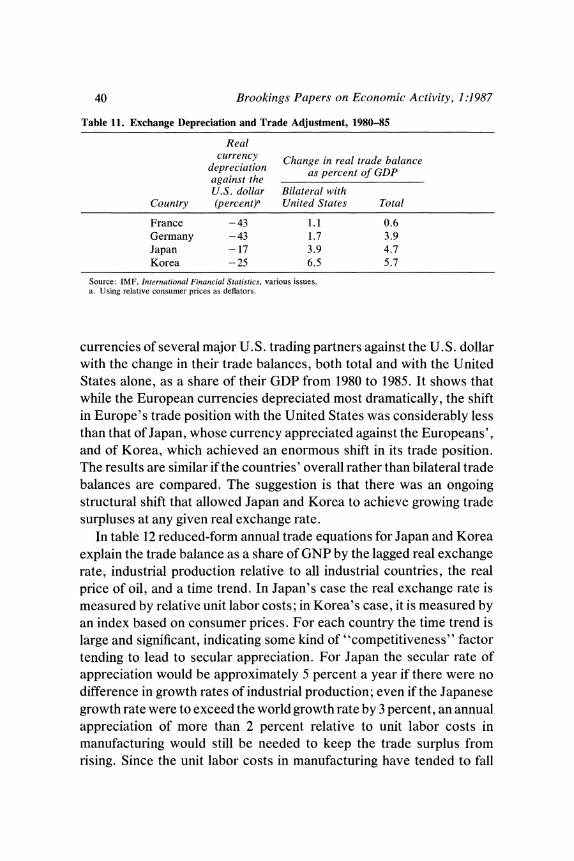
40 Brookings Papers on Economic Activity, 1:1987
Table 11. Exchange Depreciation and Trade Adjustment, 1980-85
Real currency Change in real trade balance
depreciation as percent of GDP against the U.S. dollar Bilateral with
Country (percent)a United States Total
France -43 1.1 0.6 Germany - 43 1.7 3.9 Japan -17 3.9 4.7 Korea - 25 6.5 5.7
Source: IMF, International Financial Statistics, various issues. a. Using relative consumer prices as deflators.
currencies of several major U. S. trading partners against the U. S. dollar with the change in their trade balances, both total and with the United States alone, as a share of their GDP from 1980 to 1985. It shows that while the European currencies depreciated most dramatically, the shift in Europe's trade position with the United States was considerably less than that of Japan, whose currency appreciated against the Europeans', and of Korea, which achieved an enormous shift in its trade position. The results are similar if the countries' overall rather than bilateral trade balances are compared. The suggestion is that there was an ongoing structural shift that allowed Japan and Korea to achieve growing trade surpluses at any given real exchange rate.
In table 12 reduced-form annual trade equations for Japan and Korea explain the trade balance as a share of GNP by the lagged real exchange rate, industrial production relative to all industrial countries, the real price of oil, and a time trend. In Japan's case the real exchange rate is measured by relative unit labor costs; in Korea's case, it is measured by an index based on consumer prices. For each country the time trend is large and significant, indicating some kind of "competitiveness" factor tending to lead to secular appreciation. For Japan the secular rate of appreciation would be approximately 5 percent a year if there were no difference in growth rates of industrial production; even if the Japanese growth rate were to exceed the world growth rate by 3 percent, an annual appreciation of more than 2 percent relative to unit labor costs in manufacturing would still be needed to keep the trade surplus from rising. Since the unit labor costs in manufacturing have tended to fall

Paul R. Krugman and Richard E. Baldwin 41
Table 12. Reduced-Form Trade Balance Equations, Japan and South Korea, 1969-85a
Independent variable South and summary statistic Japan Korea
Lagged real exchange rate -0.111 -0.171 (0.025) (0.066)
Relative industrial production - 0.087 0.021 (0.053) (0.042)
Real price of oil -0.029 -0.103 (0.008) (0.026)
Time trend 0.006 0.014 (0.001) (0.006)
Summary statistic K2 0.81 0.81 Standard error 0.007 0.02 Durbin-Watson 1.62 1.60
Source: Authors' calculations using data from IMF, International Financial Statistics. See text description. a. Dependent variable is the ratio of the trade balance to GNP in each country. Real exchange rates are relative
unit labor costs for Japan, ratio of consumer prices to world export prices for South Korea. Relative industrial production is the ratio of domestic to world industrial production. The real price of oil is the ratio of the Ras Tanura price to world export prices. Numbers in parentheses are standard errors.
relative to the economywide price level, the required appreciation would be even larger by most other measures. In Korea's case the required appreciation is a remarkable 10 percent a year.
The distinctive feature of Japan and Korea is their unusually high rates of productivity growth. Thus the evidence is consistent with the view that the historical need for continuing dollar decline is related to the rapid rise in relative productivity and technological capacity of U.S. trading partners, especially those in Asia.
HYSTERESIS
Many observers have wondered whether the markets lost by the United States as a result of the dollar's strength can be recaptured simply by bringing the dollar back to its previous level. They have worried about some form of irreversibility, in which foreigners, once having incurred the marketing and distribution costs necessary to establish beachheads in U.S. markets, are difficult to dislodge. They worry too that U. S. firms, having given up and abandoned their beachheads abroad, will find them difficult to regain. We have offered a formalization of this concern with models of "hysteresis" in the trade balance.

42 Brookings Papers on Economic Activity, 1:1987
Table 13. Tests for Hysteresis, Selected Periods, 1977:2.1986:4a
Independent Export Import Export Import variable and volume volume volume volume
summary statistic (1) (2) (3) (4)
Real expenditure 2.19 2.85 2.33 2.91 (0.12) (0.14) (0.14) (0.13)
Real exchange rate - 1.59 0.85 - 1.38 0.88 (0.12) (0.14) (0.12) (0.14)
Dummy variable 0.08 0.007 0.029 -0.013 (0.02) (0.021) (0.024) (0.019)
Summary statistic Standard error 0.028 0.028 0.033 0.028 Durbin-Watson 1.07 1.33 0.78 1.36 K2 0.94 0.99 0.92 0.99
Source: Authors' calculations. See text and tables 1-5. a. The equations estimated are reestimates of the export and import volume equations in tables 1 and 2 with two
alternative dummy variables added, one equal to 1.0 beginning in 1984:3 (first two columns) and the other equal to 1.0 beginning in 1985:2 (last two columns). Numbers in parentheses are standard errors.
The idea of hysteresis resulting from the sustained strength of the dollar seems highly plausible and is supported by numerous anecdotes. We have not, however, found clear-cut evidence that hysteresis has contributed to the persistence of the U.S. trade deficit.
Table 13 reports tests of the proposition that the strength of the dollar has led to adverse shifts in the constant terms of the trade flow equations. We reestimate the export and import volume equations of tables 1 and 2 with two alternative dummy variables: one beginning in the third quarter of 1984, when financial markets seem to have concluded that the dollar would be strong for a prolonged time, and one beginning with the onset of dollar decline in 1985:2. Neither gives any suggestion of a shift in the constant term that adversely affects the U.S. trade position; if anything, there is afavorable shift in the export equation.
Now it is true that by late 1986 the equations were seriously under- predicting the U.S. real trade deficit; dummy variables for 1986 alone do show a negative shift. However, given that there is no sign of an adverse shift during the period of the strong dollar itself, we have to say that the evidence does not support the view of hysteresis in the trade balance.
The conclusion seems to be that the decline in the exchange rate consistent with trade balance reflects the continuation of a long-standing trend rather than a result of the strong dollar itself.

Paul R. Krugman and Richard E. Baldwin 43
Summary and Conclusions
Most of the U.S. trade deficit results from well-understood causes. Faster demand growth in the United States than in other countries would have led to a substantial deficit even if the dollar had not appreciated; lagged effects of the strong dollar continue to be a major source of the trade deficit even though the rise of the dollar from 1980 to 1985 has now been reversed. The failure of the nominal trade deficit to show improve- ment through 1986 was, however, surprising, as was the only slight improvement in the real trade balance toward the end of the year. This sluggish turnaround may be an indication that the pre-1980 secular decline in the equilibrium dollar has continued through the 1980s, although we have not found supporting econometric evidence for this view.
Several popular views about the persistence of the trade deficit may be rejected on the basis of evidence and logic. The failure of the currencies of the LDCs to appreciate against the dollar is simply not quantitatively important enough to explain the trade deficit's persistence; demand growth in foreign markets on the scale currently envisaged is not likely to be enough to balance U. S. trade. Finally, the common view that shifts in expenditure can somehow eliminate the trade imbalance without real exchange rate adjustment is not valid in a world where not all goods and services are traded.
The most important question for the future is whether the decline in U.S. technological and productivity advantage over other nations will continue to translate into a need for secular decline in the real dollar, as it did in the 1970s. This need not be the case; secular decline depends not only on lagging productivity, but on a specific kind of bias in the lag.

Comments and Discussion
Barry Bosworth: In their paper Paul Krugman and Richard Baldwin evaluate certain key issues in the debate over the causes of, and the policy response to, the recent development of a large and persistent U.S. current account deficit. That debate has revolved around three basic questions. First, to what extent can the development of a trade deficit be explained by predictable market responses to the rise in the value of the American dollar from 1981 to 1985? If traditional trade equations, which emphasize macroeconomic factors such as relative rates of income growth and relative prices, can explain the pattern of trade that has developed over the 1980s, there would appear to be little scope for the more microeconomic factors that are the focus of the debate over competitiveness.
Second, can the failure of the trade balance to improve subsequent to the decline of the dollar be attributed to normal lags in the response of exports and imports to changes in the exchange rate?
Third, is there a secular deterioration in the competitiveness of American industry in world markets-as reflected in a trend decline in the real exchange rate required to maintain any given trade balance?
Krugman and Baldwin examine these issues within the context of their own small empirical model of U.S. trade. Their model differs from others in a few respects. First, while other studies have sought to explain export and import prices as a function of the real exchange rate and then to incorporate those price indexes into equations that purport to explain trade volumes, Krugman and Baldwin use a reduced form that relates trade volumes to the real exchange rate (as measured by wholesale manufacturing prices) directly. Thus, the lag structure of their volume equations reflects both the adjustment of import prices to the exchange
44

Paul R. Krugman and Richard E. Baldwin 45
rate and the adjustment of trade volumes to prices. They find that the lag between a change in the exchange rate and its effect on imports stretches over nine quarters.
Second, the import and export equations both have very high income elasticities that tend to maximize the importance of differences in growth rates relative to exchange rates. In my own empirical experiments I have found strong evidence that the short-run cyclical income elasticity exceeds the long-run elasticity, reducing the significance of differences in secular rates of growth of demand.
Finally, the authors' equations are fitted over such a short time span, 1977-86, that it is virtually impossible to infer anything about long-term trends. I am not sure of their reason for ignoring earlier periods, since a comprehensive measure of real exchange rates using wholesale prices is available from Morgan-Guaranty and the International Monetary Fund. Other studies also have found that the structure of the trade equations has remained quite stable over a long period.
Krugman and Baldwin do not report their forecast errors in detail, but it would appear from figure 6 that the errors were small in 1985 and 1986. I would conclude that their results are in line with other recent studies in finding surprisingly little room for microeconomic factors to account for the decline in the trade balance.1 They place a greater emphasis than other studies on differences in income growth relative to exchange rates, but that is mainly because they focus on the fourth quarter of 1986, when the dollar had moved back to the 1981 level and any remaining impact of the exchange rate on trade volumes was limited to the effect of lags.
Krugman and Baldwin do find that adjustment lags cannot fully account for the failure of the trade deficit to improve in 1986. They rather substantially underpredict the trade deficit by late 1986, and they also report a forecast in which the trade deficit persists even with current exchange rates and equal demand growth in the United States and the rest of the world. They interpret these results to imply that the United States suffers from a secular decline in the real exchange rate required to maintain any given trade balance.
1. For a summary of the predictions from the trade blocks of several macroeconomic models, see Ralph C. Bryant and Gerald Holtham, "The External Deficit: Why? Where Next? What Remedy?" Brookings Review, vol. 5 (Spring 1987), pp. 28-36.
46 Brookings Papers on Economic Activity, 1:1987
I do not believe that their arguments for a secular deterioration are fully convincing. First, the failure of the trade balance to turn around can be traced largely to the failure of import and export prices to respond fully to the exchange rate decline, not to a failure of trade volumes to respond to the new prices. U.S. export prices fell about 20 percent relative to domestic output prices betwen 1982 and 1985. Krugman and Baldwin attempt to relate much of that decline to the exchange rate and expect a substantial rise in export prices as the dollar falls. Some research at the Federal Reserve by William Helkie and Peter Hooper, however, suggests that the apparent price decline is a reflection of the specific mix of products that the United States exports: an index of domestic prices using export weights showed the same magnitude of decline. On the import side the puzzle is that prices did not rise as rapidly after 1985 as would be expected on the basis of historical experience. It is not that American purchasers have failed to respond to the price change; they simply have yet to observe much of a change. It appears that trade equations based on actual export and import prices do not produce large errors in late 1986; the puzzle is explaining the failure of prices to adjust.
Second, although Krugman and Baldwin point out that the real exchange rate did fall substantially between 1970 and 1980, when the United States had a relatively constant overall current account balance, the total current account includes the impact of oil price changes that are outside the range of their analysis. The nonagricultural, nonoil balance did improve substantially in 1980, but a comparison that focuses on individual years can be misleading because of cyclical fluctuations in the United States and abroad. The more relevant type of evidence would be a negative trend in the export equation or a positive trend in the import equation-something they did not find for the 1977-86 period. They mention the use of a relative capacity variable in the Federal Reserve model, but if that is the appropriate measure there is no longer a significant difference in the growth of capacity between the United States and its major trading partners. Thus, the problem should be of reduced importance in the future.
When I estimated equations similar to those of Krugman and Baldwin, but extending from 1967 to 1987, and used the real exchange rate series published by Morgan-Guaranty, I found evidence of significant trend effects in both the export and import equations that supports their argument, but in both cases a second-order trend was also significant

Paul R. Krugman and Richard E. Baldwin 47
and opposite in sign. The overall magnitude of the effect was very small by the 1980s.
What remains is a significant difference between the income elasticity of imports and exports, although the absolute size of the long-term coefficients was much smaller than reported by Krugman and Baldwin. Thus, if the rest of the world does not, as in past decades, grow more rapidly than the United States, there is an implied requirement for a decline in the real exchange rate. Apparently, however, it results from the differences in income elasticities, and I did not find in the paper any explanation why those differences should exist.
Finally, Krugman and Baldwin project an improvement in the U.S. trade balance through 1988 but a worsening in 1989 and beyond. That forecast follows directly from their assumptions that allow the rest of the world to grow no faster than the United States. Thus, the gap between the level of demand in the United States and abroad that opened up between 1980 and 1986 is allowed to persist forever. The magnitude of any secular deterioration is actually quite small and is represented by the very slow decline in the trade balance after 1989.
More alarming is the evidence of the buildup of a large structural imbalance in the first half of the 1980s that will not be eliminated by a return of the real exchange rate to the level that existed at the beginning of the decade. The situation is even worse for the overall current account once account is taken of the interest payments that must be made on the foreign debt that the United States has accumulated in the 1980s.
Peter Hooper: Krugman and Baldwin have two explanations for the persistence of the U.S. trade deficit. One concerns adjustment lags: for a variety of reasons largely consistent with previous experience, trade prices have been slow to adjust to the dollar's decline, and trade volumes have been slow to adjust to changes in trade prices. This explanation suggests that a significant amount of adjustment is still to come. The other explanation concerns the authors' finding of a secular downward trend in the dollar's equilibrium real exchange rate, the exchange rate that is consistent with external balance in the long run. This explanation suggests that despite the depreciation to date, the dollar may still be substantially above its equilibrium level. The authors dismiss as rela- tively unimportant several other possible explanations, including most notably the shortfall of demand growth abroad relative to growth in the
48 Brookings Papers on Economic Activity, 1:1987
United States. They conclude that growth adjustment has only a limited role to play in correcting the U.S. external imbalance.
One's view of the world can be strongly influenced by the way one specifies one's empirical model. Unfortunately, as became painfully clear in a recent workshop on U.S. current account models held at Brookings, relatively modest changes in specification can lead to signif- icantly different views of the world, or at least of the U.S. current account. '
The paper's first conclusion, about lags, should be generally accepted. As Barry Bosworth has noted, empirical models of the U.S. current account suggest that the lags in response to exchange rate changes may well have grown longer in the recent episode of dollar depreciation. By the end of 1986 the increase in nonoil import prices was as much as 5 percent less than the predictions of the multicountry model (MCM) being used at the Federal Reserve Board. Sluggish demand abroad may well have induced foreign suppliers to absorb a more sustained decline in their profit margins than they otherwise would have, in order to maintain sales in the U.S. market.
On the issue of lags, the paper does a nice job of outlining a microeconomic basis for the price lags observed empirically. However, the authors may be too quick to discount the importance of order- delivery lags, based on their inability to find significant lags in the adjustment to income changes. The existence of significant order- delivery lags would still be consistent with this empirical result if firms in the aggregate are significantly better at predicting income than they are at predicting relative prices, which seems plausible.
Although I am generally in agreement with the paper, I would differ with the authors on three points: the trend decline in the dollar, the importance of growth factors in explaining the persistence of the trade deficit, and the pitfalls of partial-equilibrium accounting exercises.
First, the notion that the dollar must decline secularly to maintain U.S. external balance goes back at least as far as the late 1960s, when Hendrik Houthakker and Steven Magee found that the income elasticity of U.S. imports was significantly greater than the foreign income elasticity of demand for U.S. exports. This elasticity difference implied
1. See Ralph C. Bryant and others, eds., Empirical Macroeconomics for Interdepen- dent Economies (Brookings, forthcoming).
Paul R. Krugman and Richard E. Baldwin 49
that with constant relative growth rates across countries, ceteris paribus, the U.S. trade balance would decline over time.
A problem with the conventional trade equations used by Houthakker and Magee (which include only income and relative prices) is that the income coefficient picks up more than it is designed to. The tremendous growth of U.S. imports of manufactured goods from Europe and Japan between the mid-1950s and the mid-1970s, and the strong growth of imports from developing countries more recently, reflected not just the growth of U.S. demand but also a substantial increase in manufacturing output capacities abroad. For various reasons these supply-side devel- opments were not adequately reflected in relative price movements and were strongly correlated with the secular trend in income. Krugman and Baldwin attempt to deal with this specification problem by introducing a trend term. They observe a significant trend coefficient in the import equation but not the export equation. While the trend term does tend to reduce the estimated income elasticity for imports, it still leaves the conclusion that there is a downward trend in the dollar's equilibrium real exchange rate. The paper offers some explanations for this downward trend based on differences in productivity trends across countries that are not adequately captured in measures of aggregate relative prices.
My colleague Bill Helkie and I have handled this supply-side issue a little differently. Given that differences in productivity growth across countries are likely to be closely associated with differences in rates of capital formation, we introduced into our import and export equations the ratio of the stock of fixed capital abroad to fixed capital in the United States. This variable is quite significant in both the import and export equations. Moreover, it results in a lower income elasticity of U.S. imports and a higher income elasticity of U.S. exports, practically eliminating the difference between those two elasticities.
At the same time, however, movements in the relative capital stock variable differ from those of a simple time trend. During the 1960s, the growth of real fixed capital abroad exceeded that in the United States by nearly 5 percent a year on average, reflecting the continuation of postwar investment booms in Europe and Japan. In the 1970s, this growth differential was half as large, at about 2.5 percent a year, despite a surge in investment in developing countries. Since 1980, the capital stock growth differential has been reduced to well under 1 percent a year, and in the last three years the growth in capital stocks at home and abroad

50 Brookings Papers on Economic Activity, 1:1987
has been about the same. These data are admittedly crude. But they suggest that whereas a strong tendency for the dollar's equilibrium real exchange rate to decline secularly may have existed over much of the postwar period, it does not apply to more recent history.
My second difference with the authors concerns the importance of relative growth to the persistence of the trade deficit. An earlier version of Krugman and Baldwin's paper presented a model in which import and export volumes were a function of GNPs at home and abroad. The authors noted that since GNP abroad on average grew about as fast as U.S. GNP during 1980-86, a shortfall of growth abroad could not be blamed for the persistence of the deficit.
In the present version of the paper, domestic demand, or GNP minus net exports, has been substituted for GNP as the activity variable in the trade equations, with relatively little change in elasticity estimates. Since U.S. domestic demand grew substantially faster than foreign domestic demand during the early 1980s, the authors find that growth factors accounted for as much as one-third of the widening of the trade deficit. Given the structure of U.S. trade, the truth probably lies midway between these two extremes. Roughly half of U.S. trade can be classified as finished goods, for which final domestic demand would be the appropriate activity variable. The other half is raw materials and intermediate goods, for which output or GNP would be the more appropriate variable. In empirical tests with equations similar to Krugman and Baldwin's, I have found that a composite variable, which gives a weight of 0.5 to both GNP and domestic demand, performs slightly better than either GNP or domestic demand alone. In brief, the growth factor was significant, but as Krugman and Baldwin suggest, by no means dominant.
Third, I would add a note of caution about the interpretation of results from partial-equilibrium accounting exercises that attempt to quantify causal relationships among jointly determined variables. Domestic de- mand and GNP are both influenced by changes in real exchange rates, and in opposite directions. (A rise in the dollar depresses net exports and GNP, but stimulates domestic demand, while it doesjust the opposite abroad.) At the same time, the rise in the dollar itself has been attributed at least in part to the excess of domestic demand growth in the United States relative to demand growth abroad, or more specifically to U.S. fiscal expansion and foreign fiscal contraction. In the presence of such simultaneity, partial-equilibrium accounting of the effects of growth and exchange rate changes on the trade balance is at best a slippery business.
Paul R. Krugman and Richard E. Baldwin 51
Moreover, predictions of the effects of changes in exchange rates or growth on the trade balance can vary considerably when one extends the analysis to a more general framework. At a conference held at Brookings about a year ago a group of general-equilibrium multicountry models simulated the effects of an exogenous decline in the dollar. At a Brookings workshop this past January the U.S. current account sectors of many of the same models ran the same simulation. In the latter exercise, a decline in the dollar was found to have powerful positive effects on the U.S. current account in most cases. In the former exercise, the same shocks generally had much smaller effects because the decline in the dollar was allowed to influence other variables, notably incomes and prices, which depressed the rise in the current account. In the MCM we find that a given real depreciation of the dollar can have less than half the current account impact in full model simulation that it has in partial- equilibrium simulation with the current account sector. This suggests that when U.S. external imbalance adjustment takes place it will have to be accommodated by a significant shift in relative domestic demand.
Finally, absent the notion of a secular decline in the dollar, for which empirical support is mixed at best, the following implications can be drawn from Krugman and Baldwin's work. Conventional empirical models suggest that substantial reduction of the U.S. trade deficit could involve a significant further depreciation of the dollar at some point, though not necessarily. The size of the depreciation required would depend on the extent to which foreign growth increases relative to growth at home. If exogenous or policy-induced adjustment in the relative growth of domestic demand at home and abroad is not forthcoming, the alternatives are continued external imbalance or the possibility of a fall in the dollar significantly below its long-run equilibrium level, which would mean further adjustment costs down the road.
General Discussion
Hendrik Houthakker did not find it at all surprising that the U. S. trade deficit had not yet begun to fall. As previous research has shown, trade flows respond slowly to changes in exchange rates, and the dollar did not peak until early 1985. Houthakker inferred that improvement is forthcoming, so that policy actions intended to bring about further devaluation of the dollar would be neither necessary nor desirable.

52 Brookings Papers on Economic Activity, 1:1987
William Cline agreed with Houthakker's assessment. He noted that recent turning points in the trade balance have lagged the preceding turning points in the dollar by two years. The 1978:1 trough in the trade balance followed the 1976:1 peak in the dollar; the 1980:4 peak in the trade balance followed the 1978:4 exchange rate trough. Since the dollar peaked two years ago, improvements in the U.S. trade balance should be imminent.
Stephen Marris argued that the adverse trend in the equilibrium dollar exchange rate, which Krugman and Baldwin's paper relates to relative productivity in export sectors abroad, has probably slowed over time, just as Bosworth's comments on the paper indicate. One possible explanation for a negative but shrinking trend has to do with the evolution of consumer tastes. Initially, consumers exhibit a preference for local products so that the marginal propensity to import out of additional income is very low. At some point, tastes become more international, and the propensity to import rises. Marris suggested that the United States might be far along in this process and that U.S. consumers' marginal propensity to purchase foreign products may have neared its upper limit, whereas Japanese tastes may just be starting to become more international. On this thesis, the U. S. trade balance should improve more than historical equations predict. Shafiqul Islam took a more pessimistic view, arguing that a lack of nonprice competitiveness is largely responsible for the secular decline in the equilibrium real dollar exchange rate and that there is no reason to believe that the trend will not continue in the foreseeable future. Robert Gordon observed that the green revolution and agricultural reforms in China, which have made developing countries more self-sufficient in food and eroded the demand for U.S. agricultural exports, would have a permanent effect on the overall trade balance, though not on the nonagricultural, nonoil trade balance analyzed by Krugman and Baldwin.
There was some debate on the role of growth in foreign demand in bringing down the U.S. trade deficit. Cline agreed with Krugman and Baldwin that growth in foreign demand, and particularly growth in Japanese demand, was unlikely to have a major effect on the trade deficit. He observed that the value of U.S. exports to Japan is currently only $20 billion, so that even if each 1 percent increase in Japanese income produced a 3 percent increase in Japanese imports, a 1 percent increase in Japanese GNP would raise imports from the United States

Paul R. Krugman and Richard E. Baldwin 53
only $600 million, a drop in the bucket compared with the $170 billion U.S. merchandise trade deficit. But Richard Cooper pointed out that the general equilibrium effects of an increase in foreign demand could be much larger than this sort of calculation suggests. An increase in demand from Germany and Japan would raise raw materials prices, which would benefit the LDC suppliers of these raw materials, who in turn would demand more U.S. output.
Rudiger Dornbusch observed that different sorts of expenditure can affect the U.S. trade deficit differently. For example, in Latin America, investment demand has declined much more than total expenditure, with a correspondingly large effect on the demand for imports from the United States. Cooper expanded on this point, noting that investment goods account for a disproportionate share of U.S. exports to most parts of the world and that investment demand is more closely linked to changes in expenditure than to the level of expenditure, so that foreign demand stimulation could have a more beneficial effect than Krugman and Baldwin's regressions suggest.
Ralph Bryant reported on simulations of a number of world macro- economic models conducted for aJanuary symposium held at Brookings. The simulations showed that increased foreign demand could make a substantial contribution to reducing the trade deficit. According to a weighted average of the simulation results, if foreign demand grows 1 percentage point faster than U.S. demand, the U.S. trade deficit would fall $17 billion after three years and $42 billion after five years. The same models estimate that an additional 10 percent depreciation of the dollar against the yen and the European Monetary System currencies could be expected to yield a $26 billion improvement in the U.S. current account in three years and a $35 billion improvement in five years. The effects of foreign growth are of the same order of magnitude as those presented by Krugman and Baldwin, but, unlike the authors, Bryant regarded them as sizable and viewed the assumed faster growth of foreign demand as realistically achievable.
Marris argued that the authors may have given up too easily on the hysteresis idea, and did not attach much significance to the fact that the post-1984 dummy in Krugman and Baldwin's trade equations was not statistically significant. A firm that wishes to market its products in another country must make significant investments, including expendi- tures on market research and product design change. He reasoned that

54 Brookings Papers on Economic Activity, 1:1987
these investments are unlikely to be abandoned quickly in response to exchange rate changes. He noted that the failure of import prices to respond fully to the exchange rate might represent one sign that hysteresis effects are operating. William Nordhaus reasoned that the implications of hysteresis effects are important not only for understanding the lags in the trade balance but, more important, for assessing the true costs of the policies that led to the overvalued dollar. If the competitiveness of exposed U.S. industries has been permanently damaged because in- vestment and technical progress by U.S. firms were slowed by the high dollar, then the long-run costs could be substantially greater than just the future costs of servicing the foreign debt on the accumulated trade deficits of the period. Edmund Phelps pointed out that customer-market models imply that the dollar would now have to stay below normal levels for some time for the United States to regain its competitive position. He was skeptical that policymakers would allow this to happen.
One striking feature of Krugman and Baldwin's analysis, Cooper noted, is the sluggishness in the dollar price of U.S. imports when the dollar appreciates or depreciates. The conventional interpretation, Cooper continued, is that foreign producers' profit margins fatten when the dollar appreciates and shrink when it depreciates. But even the best available import price data ignore changes in the ancillary terms offered by foreign suppliers associated with changes in the value of the dollar. For example, when the dollar was rising, foreign suppliers lengthened credit terms, absorbed the costs of transporting their products within the United States, and contributed to U.S. advertising budgets, all of which lowered the dollar costs of importing their products. The threat of antidumping suits made it attractive to use these devices and to keep invoice prices high. Now that the dollar has fallen, all of this is being reversed.
Catherine Mann noted that a good part of U.S. consumer goods imports comes from countries whose currency has not appreciated much against the dollar; it is therefore not surprising that the dollar prices of these imports have risen very little. In contrast, the dollar prices of capital goods imported from Europe and Japan have risen 10 to 15 percent; the increase is not proportional to the depreciation of the dollar against these currencies, but it is still substantial. In general, Mann continued, disaggregated price equations are likely to be more informa- tive than aggregate equations of the sort Krugman and Baldwin rely on.

Paul R. Krugman and Richard E. Baldwin 55
Robert Gordon added that the various price measures used in the authors' regressions and in their calculations of real exchange rates are not comparable either across countries or even within the United States. Their results are bound to be sensitive to the price indexes used. The problem is especially serious for high-technology goods, which are important in trade and for which quality improvements are treated quite differently in different price indexes.