The perfect smile Filling the gaps in the swaption volatility cube · 2020-03-18 · Filling the gaps in the swaption volatility cube 3 Market overview 2 BIS OTC derivatives statistics,

The perfect smileFilling the gaps in the swaption volatility cube

The perfect smileHow to deal with missing swaption volatility quotes.

The perfect smile Filling the gaps in the swaption volatility cube

1

ContentsIntroduction 3

Market overview 4

Valuation 101 5

Smiles, surfaces and cubes 9

The lifted swaption smile 10

Case study 12

Discussion 15

References 16


2

Introduction

1 In 2018, the monthly trading volume of swaptions was around 1 trillion USD monthly, compared to 125 million USD for caps/floors.

Liquidity of swaptions versus caps/floorsSwaptions, caps and floors are popular OTC interest rate derivatives, used by banks and corporations to manage interest rate risks arising from their core business or from their financing arrangements.

The swaption market is approximately an order of magnitude larger than the equivalent cap/floor market.1 Nonetheless, the larger market volumes do not necessarily mean that the volatility quotes are liquid in all parts of the swaption volatility cube. Indeed, one often observes that the at-the-money swaption market is very liquid, however, for various tenors and expiries, the away-from-the-money quotes are missing or not at all reliable, especially when compared to corresponding cap/floor volatilities. The reason behind this can partially be explained due to different applications of swaptions versus caps/floors.

Volatility quotes depend on hedging applications Swaptions are commonly traded to hedge against prepayment risks arising from fixed rate mortgages. Purchasing a swaption allows an issuer of a mortgage to “replace” the cash flows that would be lost in case of a prepayment. In general, prepayment is a risk when rates are declining. As a result, a prepayment hedge would often be an at-the-money (or slightly out-of-the money) swaption.

Caps/floors on the other hand are often used to hedge interest rate risk arising from contractual upper and lower rate bounds in floating-rate mortgages contracts. This would be the case, for example, in a mortgage contract which limits the variability of the floating rate from 0% to 3% (for instance). Given that the contractual bounds are typically away from the current level of interest rate, one would expect that caps/floors have liquid trades away from the money as well.

Completing the swaption volatility cubeThe portfolio of a financial institution is typically very complex with instruments that require a range of volatility quotes. Therefore, although the data providers may not give quotes on the entire volatility cube, the trading floor and risk management of the financial institution are obliged to complete it.

How to fill the gaps in the swaption volatility cube?There are several different ways by which one can “complete” the swaption volatility cube. The most common approach is based on the SABR model, which provides a way of interpolating volatilities between quoted strikes, as well as extrapolating beyond them. The SABR parameters (alpha, beta, rho and nu) can be easily calibrated when the market provides a number of reliable volatility quotes at different strikes, for a fixed expiry and tenor (see Skantzos et al. (2016)).

When, however, for a given expiry and tenor, one only has one quoted strike (typically the at the money point), the SABR approach cannot be applied directly. In this case, additional assumptions need to be made. Typical approaches would be to crudely assume a flat volatility smile, or to leverage some of the smile characteristics observed for different tenors or expiries (in case they would be available). This article, however, focuses on an alternative approach: using the information available from the cap/floor volatility surface to inform a swaption volatility smile.

Lifting from capsThere exists an intricate relationship between swaptions and caps/floors. Indeed, both instruments reference the same underlying interest rate curve. Whereas swaptions relate to forward swap rates, caplets/floorlets are driven by changes in forward rates. This relationship between the two instruments can be used to inform a swaption volatility smile from the cap/floor volatility surface, an approach referred to as: “lifting from caps”. In this article, we explore two different market practices: • Lifting from SABR (Hagan et al. (2004)): the SABR beta, rho and nu SABR parameters are taken from the caplet market. The alpha parameter is recalibrated to match the quoted at the money swaption volatility.

• A structural approach: an explicit relationship is made between cap/floor volatilities and swaption volatilities by expressing the forward swap rate as a series of forward rates.

In this article, we present the key ideas and features of the two approaches, and illustrate the two approaches on the EUR swaption market.


3

Market overview

2 BIS OTC derivatives statistics, Q2 2018.3 In 2018, the average monthly volume of Swaptions cleared at CME was 30 billion USD, compared to the total monthly volume of over 1 trillion USD.

Quick Recap: Swaptions, caps and floorsSwaptions, caps and floors are interest rate derivatives that provide a protection against an adverse move in rates whilst allowing for a benefit from an upside. Banks and corporations typically use such interest rate derivatives to manage interest rate risks arising from their core business or from their financing arrangements.

A swaption provides the investor the right but not the obligation to enter into a pre-defined interest rate swap at a fixed future date. As the name suggests, a swaption is essentially comprised of two key components: the “option component” and the “swap component”. The “option” component specifies the date at which the optionality can be exercised (the expiry). The “swap” component outlines the contractual features of the referenced swap: the underlying interest rate index, the fixed swap rate (strike), and the maturity of the swap (the tenor). We point out the two key time dimensions for swaptions: the expiry and the tenor.

An interest rate cap is in essence a series of call options (caplets) on a floating interest rate index, usually 3 or 6 month Libor. In other words, the owner of the cap receives payments at the end of each period equal to the positive part of the difference between the observed rate and a fixed strike. Similarly, an interest rate floor is a series of put options (floorlets) on an underlying interest rate index. In contrast to the swaption, caps and floors only have one time dimension: the expiry of the option (i.e., the expiry of the last caplet or floorlet).

Market overview: the main OTC interest rate derivativesAs of June 2018, the global interest rate derivatives market had an outstanding notional of 481 trillion USD2. The lion share (70%) of this market is comprised of interest rate swaps. A non-negligible 10% of this market, however, is comprised of interest rate options such as swaptions, caps/floors and more exotic derivatives.The monthly trading volume of the interest rate options market is approximately 1.5 trillion USD, two thirds of which comes from swaption trades and a further 125 billion USD from the cap/floor market.

Up until recently, both the swaption and cap/floor market were uncleared markets. In 2016, however, CME started clearing swaptions. Nonetheless, the cleared swaption market only comprise a small minority of the total swaption transactions3.

Swaption and caps as hedging instrumentsAs outlined above, the swaption market is almost 10 times larger than the cap/floor market. Part of the reason behind this difference in market size lies in the application of caps, floors and swaptions in

hedging various interest rate risks.

Swaptions are frequently used to hedge against early termination features in fixed rate paying instruments, such as callable bonds or prepayment options in fixed rate mortgages. Typically a fixed rate mortgage holder would consider prepaying when the interest rates decline. Purchasing a swaption allows a financial institution to “replace” the future interest rate payments that would be lost in case of a mortgage prepayment (or in the case of a bond being called).

Swaptions also are a popular tool for liability-driven investors, such as pension funds, who rely on fixed-income asset returns to meet their future liabilities. In this case, a swaption would allow pension funds to protect their funding in case of a decline in interest rates.Interest rate caps and floors, on the other hand, are typically used to hedge contractual upper and lower bounds in variable rate instruments. For example, many variable rate mortgages contracts contain an embedded cap or floor on the interest rate (e.g., the rate a borrower pays cannot exceed a maximum of X%, but also cannot go below a minimum of Y%). A contractual lower bound covers any costs of the issuer associated with processing and servicing the loan, whereas an upper bound protects the borrower against extreme increases in rates. Hedging these contractual features in the variable rate instruments hence requires issuing or purchasing of caps and floors

In general, the variable rate instrument market is smaller than its corresponding fixed rate market. For example, in the US, variable rate mortgages comprise around 10% of the total mortgage market (the remaining 90% being fixed rate). Since swaptions are used to hedge fixed rate instruments, the popularity of fixed rate mortgages over variable rate mortgages can help explain (at least in part) the higher liquidity of the swaption market.

Swaptions are used to hedge prepayments in fixed rate instruments, whereas caps/floor hedge contractual features in variable rate mortgages.


4

Valuation 101

4 The swap rate of a swap is the fixed rate that makes the swap value equal to zero at time t.

Key ingredients for pricing caps, floors and swaptionsDetermining the price of a swaption, cap or floor requires a number of key ingredients. First, one needs to know all contractual features of the option (underlying interest rate, maturity, strike, etc.). Second, one requires the current level of the relevant interest rate. In the case of a swaption, this would be the forward swap rate of the referenced swap, whereas for caps/floors, the relevant rate is the forward interest rates corresponding to the different caplet/floorlet fixing dates. Finally, one requires a pricing model that determines the likelihood of upwards or downward movements in the interest rate, in other words one requires an estimate for the interest rate volatility.

Caps/FloorsValuation ingredients

SwaptionsValuation ingredients

Notional Notional

Strike Strike

Underlying instrument (e.g. the Euribor 6M)

Underlying instrument (e.g. the Euribor 6M)

Expiry of the cap (payment date of the last caplet,)

Maturity of the option (referred to as “expiry”)

Start/End of swap (referred to as “tenor”)

Cap or Caplet Volatilities Swaption Volatility

Forward rate at each caplet payment date

Forward swap rate for the option expiry

Discount curve (OIS) Discount curve (OIS)

Because of the extra time component that is required to value a swaption (the “tenor”), the swaption volatility is a higher-dimensional object than a cap volatility. This is one of the reasons, why mapping cap vols to swaption vols is not a trivial task. A mathematically more intuitive explanation follows in the section below.

Swaption market versus cap marketFrom an algebraic point of view, a cap/floor and a swaption have very similar payoffs involving an optionality (the positive part of the

difference between a forward rate and a strike) and a summation. They differ, however, in the order by which these two occur in the payoff. This difference is responsible for the absence of a one-to-one mapping between the two payoffs. For more details, see the Digression table next.

Forward rate versus forward swap rateThe key difference between caps/floors and swaptions is that the underlying of the former is an -IBOR rate, whereas the latter references a swap rate. Consequently, the valuation of a cap/floor requires as input a forward rate whereas the equivalent input for the swaption is the forward swap rate.

The forward rate, F(t,T,S), corresponds to the market expectation at valuation date t of a the future IBOR-rate, that will be fixed at time T with tenor S-T. The forward swap rate, S(t,T1,Tn ), on the other hand, corresponds to the market expectation at valuation date t of the swap rate4 starting time T1 and maturing at Tn.There exists an intricate relationship between the forward rate and the forward swap rate, as shown in the table below:

Relationship between forward rate and forward swap rate

A forward swap rate is in essence a weighted average of forward rates. This relation is the starting point for the “structural” approach for connecting the swaption and cap markets.

where

and we have used the following notation• τa,b is the year-fraction between times a and b• P(t,T) is the (OIS) discount factor between time t and T

These relations will be important in the subsequent sections, and in particular, the following relation between the two forwards. This will be the starting point of the structural approach connecting the swaption to the cap volatility cubes.


5

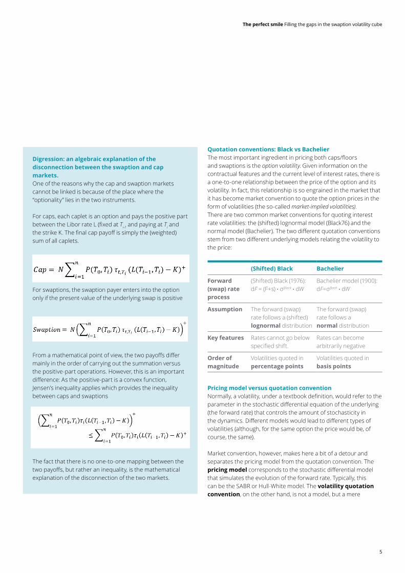
Quotation conventions: Black vs BachelierThe most important ingredient in pricing both caps/floors and swaptions is the option volatility. Given information on the contractual features and the current level of interest rates, there is a one-to-one relationship between the price of the option and its volatility. In fact, this relationship is so engrained in the market that it has become market convention to quote the option prices in the form of volatilities (the so-called market-implied volatilities).There are two common market conventions for quoting interest rate volatilities: the (shifted) lognormal model (Black76) and the normal model (Bachelier). The two different quotation conventions stem from two different underlying models relating the volatility to the price:

(Shifted) Black Bachelier

Forward (swap) rate process

(Shifted) Black (1976):dF = (F+s) . σBlack . dW

Bachelier model (1900):dF=σBach . dW

Assumption The forward (swap) rate follows a (shifted) lognormal distribution

The forward (swap) rate follows a normal distribution

Key features Rates cannot go below specified shift.

Rates can become arbitrarily negative

Order of magnitude

Volatilities quoted in percentage points

Volatilities quoted in basis points

Pricing model versus quotation conventionNormally, a volatility, under a textbook definition, would refer to the parameter in the stochastic differential equation of the underlying (the forward rate) that controls the amount of stochasticity in the dynamics. Different models would lead to different types of volatilities (although, for the same option the price would be, of course, the same).

Market convention, however, makes here a bit of a detour and separates the pricing model from the quotation convention. The pricing model corresponds to the stochastic differential model that simulates the evolution of the forward rate. Typically, this can be the SABR or Hull-White model. The volatility quotation convention, on the other hand, is not a model, but a mere

Digression: an algebraic explanation of the disconnection between the swaption and cap markets.One of the reasons why the cap and swaption markets cannot be linked is because of the place where the “optionality” lies in the two instruments.

For caps, each caplet is an option and pays the positive part between the Libor rate L (fixed at Ti-1 and paying at Ti and the strike K. The final cap payoff is simply the (weighted) sum of all caplets.

For swaptions, the swaption payer enters into the option only if the present-value of the underlying swap is positive

From a mathematical point of view, the two payoffs differ mainly in the order of carrying out the summation versus the positive-part operations. However, this is an important difference: As the positive-part is a convex function, Jensen’s inequality applies which provides the inequality between caps and swaptions

The fact that there is no one-to-one mapping between the two payoffs, but rather an inequality, is the mathematical explanation of the disconnection of the two markets.


6

translation device that converts prices into (some) model’s volatilities and vice versa.

It is a typical case, for example, to have Black or Bachelier volatilities coming out of the SABR model. This would mean that the SABR model was used to simulate the forward rate and arrive at a caplet’s price and the output is expressed in terms of the volatility that one needs to insert to the Black formula to get the price. The reasons for this seemingly awkward process are historical. When the option market realized in the mid 80’s that the Black model does not capture well the stylised facts of trading (namely, the smile) new models were introduced, however, the convention of quoting prices in terms of Black (or Bachelier) vols remained.

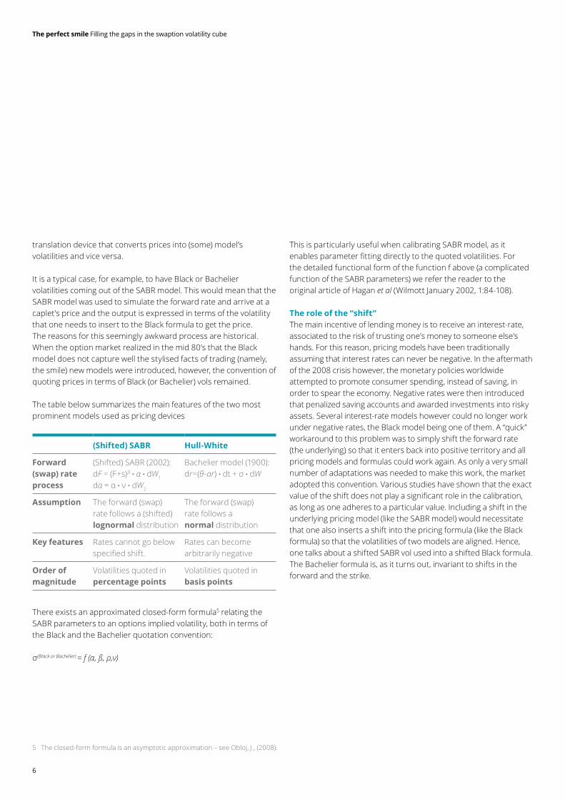
The table below summarizes the main features of the two most prominent models used as pricing devices

(Shifted) SABR Hull-White

Forward (swap) rate process

(Shifted) SABR (2002):dF = (F+s)β . α . dW1

dα = α . ν . dW2

Bachelier model (1900):dr=(θ-ar) . dt + σ . dW

Assumption The forward (swap) rate follows a (shifted) lognormal distribution

The forward (swap) rate follows a normal distribution

Key features Rates cannot go below specified shift.

Rates can become arbitrarily negative

Order of magnitude

Volatilities quoted in percentage points

Volatilities quoted in basis points

There exists an approximated closed-form formula5 relating the SABR parameters to an options implied volatility, both in terms of the Black and the Bachelier quotation convention:

σ(Black or Bachelier) = f (α, ß, ρ,ν)

5 The closed-form formula is an asymptotic approximation – see Obloj, J., (2008).

This is particularly useful when calibrating SABR model, as it enables parameter fitting directly to the quoted volatilities. For the detailed functional form of the function f above (a complicated function of the SABR parameters) we refer the reader to the original article of Hagan et al (Wilmott January 2002, 1:84-108).

The role of the “shift”The main incentive of lending money is to receive an interest-rate, associated to the risk of trusting one’s money to someone else’s hands. For this reason, pricing models have been traditionally assuming that interest rates can never be negative. In the aftermath of the 2008 crisis however, the monetary policies worldwide attempted to promote consumer spending, instead of saving, in order to spear the economy. Negative rates were then introduced that penalized saving accounts and awarded investments into risky assets. Several interest-rate models however could no longer work under negative rates, the Black model being one of them. A “quick” workaround to this problem was to simply shift the forward rate (the underlying) so that it enters back into positive territory and all pricing models and formulas could work again. As only a very small number of adaptations was needed to make this work, the market adopted this convention. Various studies have shown that the exact value of the shift does not play a significant role in the calibration, as long as one adheres to a particular value. Including a shift in the underlying pricing model (like the SABR model) would necessitate that one also inserts a shift into the pricing formula (like the Black formula) so that the volatilities of two models are aligned. Hence, one talks about a shifted SABR vol used into a shifted Black formula. The Bachelier formula is, as it turns out, invariant to shifts in the forward and the strike.


7

Smiles, surfaces and cubesSwaption volatility cube versus cap/floor volatility surfaceCaps, floors and swaptions are quoted at different strike levels. The graphical representation of the implied option volatility at different strikes is known as the volatility smile.

Recall that for swaptions there are two time dimensions: the swaption expiry and swaption tenor. Adding these two time dimensions to the strike dimension, one has that the set of implied swaption volatilities comprises a three-dimensional volatility cube. Caps and floors, on the other hand, only have one time dimension: the expiry. In this case, one speaks of a two-dimensional volatility surface.

The swaption volatility cube and cap volatility surface form the basis for calibrating any interest rate models (e.g., SABR, Libor Market Model, Hull-White, etc.). Ensuring reliable volatility information across the whole surface/cube is hence the starting point for any interest rate modelling.

From cap vols to caplet volsA cap represents a series of caplet options. Each caplet is linked to the forward rate of the start/end dates of that caplet. In order to price each caplet the volatility of the corresponding forward rate is required. In practical terms, this would mean that for trading a cap one may need to communicate a long series of caplet vols, especially for long maturity caps.

The market circumvents this tedious process by an efficient one: regardless of the number of caplets in a cap, the market communicates one single volatility number, which is the cap vol. This represents a fictitious caplet volatility that if inserted across all caplets would result in the correct cap price. Thus, a cap vol is a short-hand for the price that can be quoted for all strikes and maturities. In fact, this is the traded quantity, rather than the caplet vol.

The SABR model however outputs caplet vols (Black or Bachelier), not cap vols. Therefore, to calibrate the SABR model one first needs to convert the market quoted cap vols into caplet vols. This procedure of extracting the caplet volatility surface from the cap volatility surface requires an intricate bootstrapping procedure called caplet stripping.

In the swaption market, things are fortunately far simpler. The swaption volatility represents exactly the volatility of the swaption’s underlying forward swap rate. The swaption volatility cube can hence directly be used for swap rate modelling.

Digression: Stripping caplet volatilitiesObtaining the caplet volatility surface requires reliable quoted cap volatilities at various expiries and strikes. Extracting the caplet volatility surface from the quoted cap volatilities consists of four steps (Skantzos et al. (2016)):

1. Converting cap volatilities to pricesIn a first step, the cap volatilities are converted into cap prices by applying the (shifted) Black formula or Bachelier formula (depending on whether the volatility quotation is (shifted) lognormal or normal).

2. Stripping caplet volatilitiesUsing a bootstrapping procedure across the cap expiries, individual caplet prices are inferred from the cap prices. The stripped caplet prices are in turn converted to caplet volatilities.

3. Calibrating SABR on caplet market For each caplet expiry, one calibrates the SABR model on the caplet volatilities determined in step 2. One obtains a set of SABR parameters for each option expiry τ (ατ

caplet, βτ

caplet, ρτcaplet and ντ

caplet).

4. Interpolating/extrapolating caplet volatility smile Using the asymptotic approximations to the SABR model outlined by Obloj (2008), one has a closed-form expression of the caplet volatility smile for each expiry ?.


8

Missing quotes and market liquidityIn a modeller’s ideal world, the market would liquidly quote option volatilities throughout across all strikes, maturities and tenors. Unfortunately, in reality only small parts of the volatility surface/cube are actually liquidly traded.

Despite the swaption market being the larger market, it is not the case that the swaption volatility cube is more liquid at each point compared to the cap/floor volatility surface. First of all, there are more possible different combinations of swaptions, as they have an additional time dimension; the swaption tenor. Secondly, the swaption market liquidity is not evenly spread across the different strikes. Indeed, one has that at the money swaptions (i.e., strike equal to current forward swap rate) are far more liquidly traded than those away from the money.

In the cap/floor market, one also has that at the money options are typically more liquid. In contrast to the swaption market, however, cap/floor volatilities are more regularly quoted for a number of in-the money and out of the money strikes.

One reason behind this difference in liquidity “at the money” versus “away from the money” lies in the different applications of swaptions and caps/floors in the context of interest rate risk hedging. As discussed previously, swaptions hedge against early terminations in fixed rate mortgages or bonds. When issuing a fixed rate mortgage or bond at the current market rate, one would like to ensure that one receives this rate, even in the case of an early termination. This insurance would be exactly an at the money swaption. Caps and floors, on the other hand, hedge against contractual caps/floors embedded in the contracts of variable rate instruments. These embedded caps/floors are typically away from the money. For example, in a variable rate mortgage, the contractual floor is typically below the current market rate and the contractual cap is above the current market rate.

Different applications of swaptions versus caps/floors in the context of interest rate risk hedging help explain why swaption quotes are more concentrated at the money.

Completing the swaption volatility cubeWhen interest rate quants and traders are faced with unreliable or missing swaption volatility quotes, they need to find ways to interpolate or extrapolate information in order to “complete” their volatility cube.

There are several different ways by which one can “complete the cube”. The most common approach is via the SABR model, which provides an expression for the volatility smile for a given tenor and expiry. Given a tenor and expiry combination, one calibrates the SABR parameters (alpha, beta, rho, nu) on the quoted strikes, enabling interpolation between market quotes, as well as extrapolation to far out of the money and in the money options (see Skantzos et al. (2016)).

Unfortunately, the SABR calibration only works when volatilities are quoted for a number of different strikes. When, however, for a given expiry and tenor, one only has a single volatility quote (typically the at the money point), the SABR approach cannot be applied directly. In this case, additional assumptions need to be made.

Typical approaches include crudely assuming a flat volatility smile, or leveraging smile characteristics observed for different tenors or expiries (in case they would be available). In the following section, we look at an alternative approach in which the information from the caplet volatility surface is used to inform a swaption volatility smile.


9

The lifted swaption smileIn this section, we discuss two different approaches used in practice to inform the swaption volatility surface from the cap market. Both approaches assume a prior calibration of a full volatility surface for the caplet market. That is, for each expiry T and strike K, one has a caplet volatility: σT

caplet (K)expressed in terms of the four SABR parameters α caplet (T),βcaplet (T),ρcaplet (T),νcaplet (T) and the corresponding shift that is used.

In addition to the availability of a caplet volatility surface, both approaches assume a reliable at the money (ATM) swaption volatility quote. As discussed in the previous section, these are typically available, as ATM swaptions are liquidly traded for most expiries and tenors.

Approach A: Lifting SABR parameters Hagan et al. (2004) outline an approach in which caplet SABR parameters are used as the basis for calculating the swaption volatility cube.

The approach assumes that the swaption volatility smile is given by a SABR model with parameters: α swapt (T),βswapt (T),γswapt (T) and νswapt

(T). The SABR parameters are determined as follows:

• The parameters βswapt (T),γswapt (T) and νswapt (T) are set equal to the SABR parameters from the caplet smile with the same option expiry.

• The α swapt (T) parameter is calibrated such as to match the quoted ATM swaption volatility.

Effectively, as βswapt (T),γswapt (T) and νswapt (T) are understood to determine the shape of a smile, one assumes that the convexity and level of symmetry of a swaption smile is identical to that of a caplet smile. A parallel shift (impacted by the recalibration of αswapt (T)) would ensure to give back the correct ATM quote. An explicit expression for the resulting swaption smile is then obtained from the asymptotic approximations to the SABR model (Obloj 2008).

Approach B: Structural approachIn this approach, an explicit relationship is made between cap/floor volatilities and swaption volatilities by expressing the forward swap rate as a series of forward rates. For illustration purposes, we present the example of a swaption with a 1-year tenor on the 6M Euribor rate. The calculation, however, works similarly for other tenors.

Step 1: Expressing the forward swap rate in terms of forward ratesFirst, the referenced forward swap rate is expressed as a linear combination of forward rates. For a swaption with expiry T and tenor 1Y, we have that the referenced swap rate equals:

where, as before: • τ(a,b) denotes the yearfraction between times a and b. • P(t,T) is the (OIS) discount factor, discounting the payment at time T back to t (t, being the valuation date).

• FT¬>T+6M(t) is the forward rate between T and T + 6M, as seen from the valuation date t, i.e. FT¬>T+6M(t)=F(t,T,T + 6M). Similarly for FT¬>T+1Y(t).

Step 2: Relating caplet volatilities to the swaption volatilityWe assume that the forward rates are normally distributed (Bachelier) with a normal (caplet) volatility.


10

Furthermore, we assume that the correlation between the two Wiener process dW1 and dW2 is ρ. The details of the deterministic part of the above two relations depend on the measure on which the two forwards are expressed. This, however, will turn out to be irrelevant for the derivations below, which are impacted only by the stochastic part. In order to see how the above two stochastic differential equations combine to produce one for the forward swap rate we employ Ito’s lemma. From equation (1), we obtain at leading order:

In the above expression, we have ignored the higher order terms, which stem from the fact that the weights w6M and w1Y are not exactly constant, but exhibit a dependence on the interest rate through the discount factor.

Since the forward rates FT¬>T+6M and FT+6M¬>T+1Y are assumed to be normally distributed, we obtain from equation (2) that the forward swap rate is also normally distributed, with some volatility σ swptn

(T x 1Y)

. Substituting the stochastic differential equations into equation (2), squaring and taking expectations leads to ( Jäckel et al. (2000)):

To lighten the notation above we have omitted the strike dependence, which needs to appear in all of the three volatilities. Several assumptions can be made as to the exact functional form of this strike dependence:

• Constant strike assumption: for a swaption with (swaption) strike K, one applies caplet volatilities with caplet strike K, i.e. the functional dependence of the left- and right-hand side of equation (2) on the strike has the form:

• Constant moneyness assumption: for a swaption with (swaption) strike K, one applies caplet volatilities for which the caplet strike has the same moneyness. In other words, if the swaption vol refers to an ATM strike (K=S), then the corresponding caplet vols refer to ATM (caplet) strikes (K=F). The functional dependence of the left- and right-hand side of equation (2) on the strike then takes the form:

In what follows, we apply the “constant moneyness” assumption, however, a similar analyses can be performed for the constant strike assumption.

Step 3: Implying Rho from the ATM Swaption volatilityAt this stage, the parameter ρ is unknown. Note, however, that we have not yet used the ATM swaption information. The correlation parameter is fixed by imposing that the T x 1Y swaption smile must go through the quoted ATM point. Let us denote this point as σATM=σswptn

(T x 1Y) (K=ST x 1Y (t)). The correlation parameter is then obtained by evaluating expression (2) with strike equal to the forward swap rate (K=ST x 1Y(t)). We have:

By inserting the calibrated correlation parameter ρ into equation (3), we obtain an expression for the T x 1Y swaption volatility smile (assuming the correlation does not have any strike dependence).


11

Case studyWe illustrate the two “lifting from caps” approaches outlined in the previous section by means of a practical application to the 6M EURIBOR market. In the EUR market, Bloomberg provides cap volatility quotes at various strike levels for most relevant expiries. For swaptions, on the other hand, Bloomberg provides ATM volatility quotes for a wide range of tenors and expiries, however only quotes volatilities away from the money for the 2Y, 5Y, 10Y, 20Y and 30Y tenors. We apply the two “lifting from caps” approaches discussed in Section 5 to infer the volatility smile for 1Y tenor swaptions, from the cap market. As a benchmark approach, we compare the “lifting from caps” approaches to a “lifting from swaptions” approach where the 1Y tenor swaption smile is informed from 2Y tenor swaptions. The three approaches are summarised in Table 1 below.

Approach Smile inferred from

Description

A “Lifted from SABR” Cap market SABR parameters beta, rho and nu are taken from the caplet volatility smile for the same expiry. The alpha parameter is recalibrated to match the ATM quote (as outlined in Section 5).

B “Structural approach” Cap market The structural relationship between the forward swap rate underlying the swaption and its comprising forward rates is used to prescribe a relationship between the swaption vols and caplet vols (as outlined in Section 5).

C “Lifted from Swaptions” Swaption market with 2Y tenor

SABR parameters beta, rho and nu are taken from the corresponding 2Y tenor volatility smile. The alpha parameter is recalibrated to match the ATM quote.

Table 1: Overview of “swaption smile lifting” approaches

The displayed 1Y tenor results below can (unfortunately) not be compared to a quoted swaption volatility smile, as this is not provided by Bloomberg. It is reasonable to assume, however, that the lifted from swaptions is “closest” to reality, as it uses the best available market data (i.e., it leverages information from the Swaption market). As both the “lifted from SABR” approach and the structural approach take the smile characteristics from the cap market, they will not be able to reflect the differences in market liquidity and market demand between the swaption and cap markets.

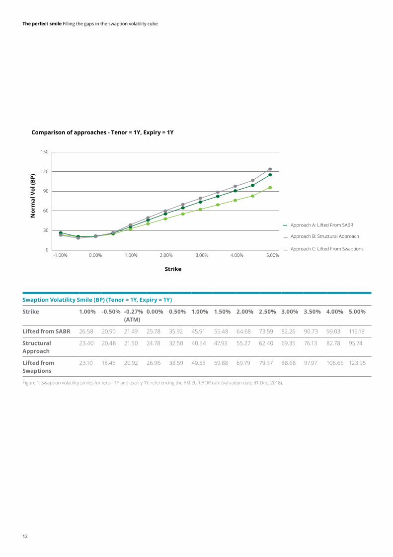
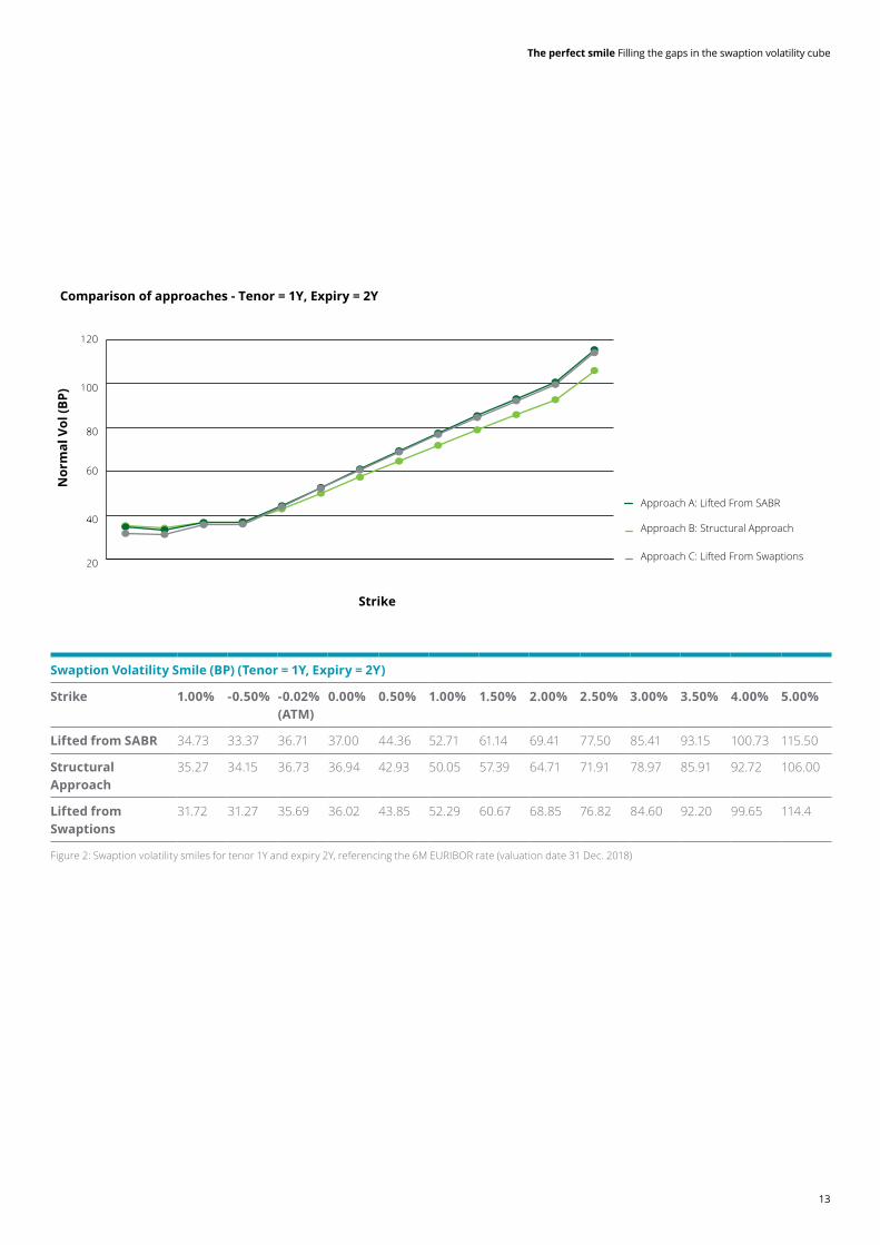
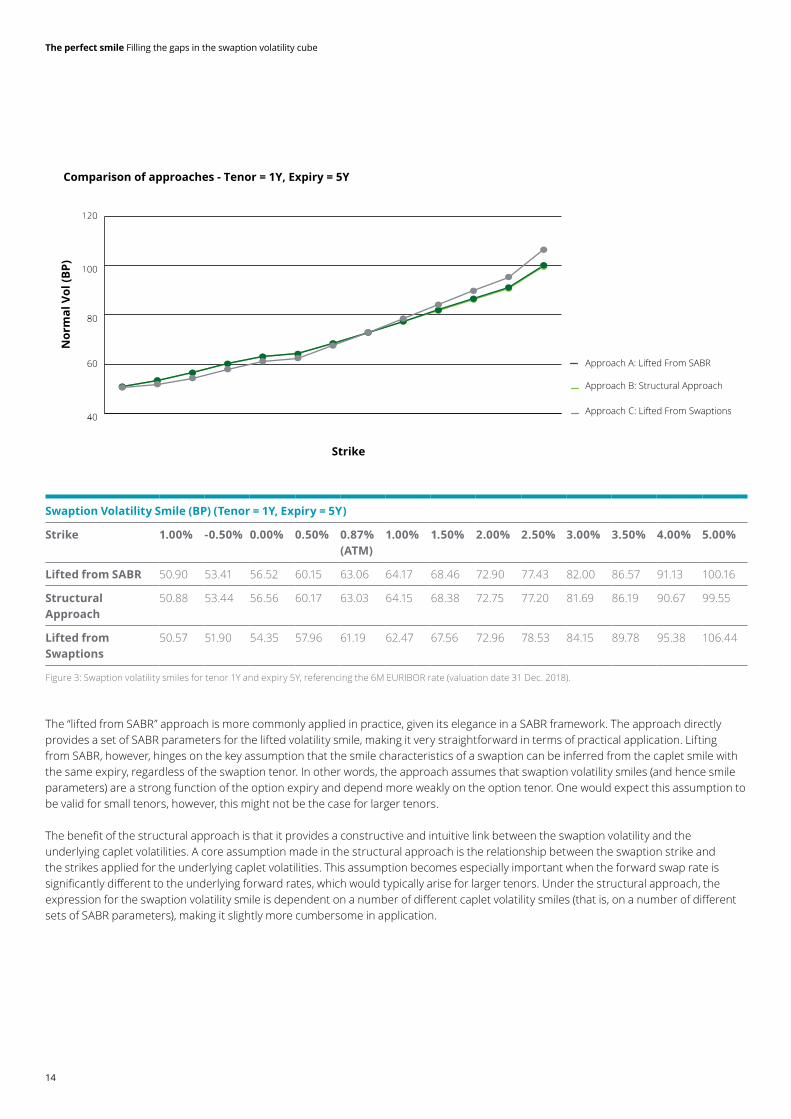
Figure 1, Figure 2 and Figure 3 below show the 1Y tenor swaption smiles for the 1Y, 2Y and 5Y expiries under the three “smile lifting” approaches. The two “lifting from caps” approaches are depicted in dark green (“lifted from SABR”) and light green (“structural approach”). The grey line corresponds to the benchmark “lifted from Swaption” approach.

It comes to no surprise that the three approaches lead to very similar volatilities near the at the money point. Interesting is to see, however, that also away from the money, we observe a reasonably good alignment between the different approaches. These observations provide a certain level of comfort regarding the model risk involved in extrapolating swaption volatilities for different tenors. We do point out, however, that one would expect the difference between the approaches to differ more significantly for larger swaption tenors.


12

Swaption Volatility Smile (BP) (Tenor = 1Y, Expiry = 1Y)

Strike 1.00% -0.50% -0.27% (ATM)

0.00% 0.50% 1.00% 1.50% 2.00% 2.50% 3.00% 3.50% 4.00% 5.00%

Lifted from SABR 26.58 20.90 21.49 25.78 35.92 45.91 55.48 64.68 73.59 82.26 90.73 99.03 115.18

Structural Approach

23.40 20.48 21.50 24.78 32.50 40.34 47.93 55.27 62.40 69.35 76.13 82.78 95.74

Lifted from Swaptions

23.10 18.45 20.92 26.96 38.59 49.53 59.88 69.79 79.37 88.68 97.97 106.65 123.95

Figure 1: Swaption volatility smiles for tenor 1Y and expiry 1Y, referencing the 6M EURIBOR rate (valuation date 31 Dec. 2018).

0-1.00% 0.00% 1.00% 2.00% 3.00% 4.00% 5.00%

30

60

90

120

150

Comparison of approaches - Tenor = 1Y, Expiry = 1Y

Nor

mal

Vol

(BP)

Strike

Approach A: Lifted From SABR

Approach B: Structural Approach

Approach C: Lifted From Swaptions


13


Strike 1.00% -0.50% -0.02% (ATM)

0.00% 0.50% 1.00% 1.50% 2.00% 2.50% 3.00% 3.50% 4.00% 5.00%

Lifted from SABR 34.73 33.37 36.71 37.00 44.36 52.71 61.14 69.41 77.50 85.41 93.15 100.73 115.50

Structural Approach

35.27 34.15 36.73 36.94 42.93 50.05 57.39 64.71 71.91 78.97 85.91 92.72 106.00


31.72 31.27 35.69 36.02 43.85 52.29 60.67 68.85 76.82 84.60 92.20 99.65 114.4

Figure 2: Swaption volatility smiles for tenor 1Y and expiry 2Y, referencing the 6M EURIBOR rate (valuation date 31 Dec. 2018)


Nor

mal

Vol

(BP)

Strike





14


Strike 1.00% -0.50% 0.00% 0.50% 0.87% (ATM)

1.00% 1.50% 2.00% 2.50% 3.00% 3.50% 4.00% 5.00%

Lifted from SABR 50.90 53.41 56.52 60.15 63.06 64.17 68.46 72.90 77.43 82.00 86.57 91.13 100.16

Structural Approach

50.88 53.44 56.56 60.17 63.03 64.15 68.38 72.75 77.20 81.69 86.19 90.67 99.55


50.57 51.90 54.35 57.96 61.19 62.47 67.56 72.96 78.53 84.15 89.78 95.38 106.44

Figure 3: Swaption volatility smiles for tenor 1Y and expiry 5Y, referencing the 6M EURIBOR rate (valuation date 31 Dec. 2018).

The “lifted from SABR” approach is more commonly applied in practice, given its elegance in a SABR framework. The approach directly provides a set of SABR parameters for the lifted volatility smile, making it very straightforward in terms of practical application. Lifting from SABR, however, hinges on the key assumption that the smile characteristics of a swaption can be inferred from the caplet smile with the same expiry, regardless of the swaption tenor. In other words, the approach assumes that swaption volatility smiles (and hence smile parameters) are a strong function of the option expiry and depend more weakly on the option tenor. One would expect this assumption to be valid for small tenors, however, this might not be the case for larger tenors.

The benefit of the structural approach is that it provides a constructive and intuitive link between the swaption volatility and the underlying caplet volatilities. A core assumption made in the structural approach is the relationship between the swaption strike and the strikes applied for the underlying caplet volatilities. This assumption becomes especially important when the forward swap rate is significantly different to the underlying forward rates, which would typically arise for larger tenors. Under the structural approach, the expression for the swaption volatility smile is dependent on a number of different caplet volatility smiles (that is, on a number of different sets of SABR parameters), making it slightly more cumbersome in application.


Nor

mal

Vol

(BP)

Strike





15

DiscussionIn this article, we discussed two methods of creating a swaption volatility smile from the cap market. The first one, the “structural” approach, derives a swaption volatility from the structural link between the forward swap rate (linked to the swaption vols) to its comprising forward rates (linked to the caplet vols). To our knowledge, Jäckel and Rebonato first proposed this methodology in 2000. It offers an intuitive and mathematically clean way of linking the swaption to the cap market. The main underlying assumption refers to the correlation between the dynamics of the two forward rate processes, which is assumed to be strike-independent. Once this correlation is obtained from ATM swaption vols, a straightforward formula is applied to obtain the rest of the smile surface.

The second method, the “lifted from SABR” approach, is based on the assumption that the swaption smile bares a shape identical to that of a cap smile, differing only by a parallel shift. In reality, this is a heuristic assumption made only for convenience as it allows the practitioner to combine in a simple way the only information that is typically available, namely the caplet volatility smiles and the swaption ATM vols. It is a straightforward approach to implement.

Both the “structural approach” and the “lifted from SABR” method are applied in the industry, and serve as useful tools when completing the swaption volatility cube. In comparing the two approaches, we identify some key benefits and disadvantages. Whereas lifting from SABR is very elegant in the SABR framework, allowing for a very straightforward implementation, it assumes that swaption volatility smiles (and hence smile parameters) are a strong function of the option expiry and depend more weakly on the option tenor. One would expect this assumption to be valid for small tenors, however, this might not be the case for larger ones.

The beauty of the structural approach is that it provides a constructive and intuitive link between the swaption volatility and the underlying caplet volatilities.It does, however, require making a strong assumption in relating the moneyness of the swaption volatility to the moneyness of the underlying caplet volatilities. This assumption becomes especially important when the forward swap rate is significantly different to the underlying forward rates, which would typically arise for larger tenors.

In the case study, we compared the two approaches for the EUR 6M market in the simple case of the 1Y tenor. The results indicate that both methodologies result in very similar swaption smiles, despite the fact that their underlying starting points and assumptions are different. This provides a certain level of confidence in the assumptions underpinning the two approaches. However, as previously discussed, we would expect in general that the smiles resulting from the two approaches diverge when tenors become larger.

References

1 Brigo D. and Mercurio F., (2007), “Interest rate models- theory and practise: with smile, inflation and credit”, Springer Finance.2 Hagan, P. and Konikov, M., (2004), “Interest rate volatility cube: Construction and use”. Technical report, Bloomberg technical report.3 Jäckel, P., and Rebonato, R., (2000), “Linking Caplet and Swaption Volatilities in a BGM/J framework: Approximate Solutions”,

Quantitiative Research Centre, The Royal Bank of Scotland.4 Obloj, J., (2008), “Fine-Tune Your Smile: Correction to Hagan et al.”, Wilmott Magazine 35, 102–104.5 Skantzos, N., Van Dooren, K. and Garston G., (2016), “Risk management under the SABR model”, Deloitte white paper.6 West, G., (2005), “Calibration of the SABR model in illiquid markets”, Applied Mathematical Finance, 12(4), pp. 371-385


17

Deloitte refers to one or more of Deloitte Touche Tohmatsu Limited, a UK private company limited by guarantee (“DTTL”), its network of member firms, and their related entities. DTTL and each of its member firms are legally separate and independent entities. DTTL (also referred to as “Deloitte Global”) does not provide services to clients. Please see www.deloitte.com/about for a more detailed description of DTTL and its member firms.

Deloitte provides audit, tax and legal, consulting, and financial advisory services to public and private clients spanning multiple industries. With a globally connected network of member firms in more than 150 countries, Deloitte brings world-class capabilities and high-quality service to clients, delivering the insights they need to address their most complex business challenges. Deloitte has in the region of 225,000 professionals, all committed to becoming the standard of excellence.

This publication contains general information only, and none of Deloitte Touche Tohmatsu Limited, its member firms, or their related entities (collectively, the “Deloitte Network”) is, by means of this publication, rendering professional advice or services. Before making any decision or taking any action that may affect your finances or your business, you should consult a qualified professional adviser. No entity in the Deloitte Network shall be responsible for any loss whatsoever sustained by any person who relies on this publication.

© July 2019 Deloitte Belgium 4635

0

Contacts

Nikos SkantzosDirectorRisk AdvisoryBelgium+32 474 [email protected]

George Garston ManagerRisk AdvisorySwitzerland+41 58 279 [email protected]

Documents

The perfect smile Filling the gaps in the swaption volatility cube · 2020-03-18 · Filling the gaps in the swaption volatility cube 3 Market overview 2 BIS OTC derivatives statistics,