Embed Size (px)
Citation preview

ISSN 2282-6483
The Paradox of Fiscal Imbalances in India
Motilal Mahamallik Pareswar Sahu
Sushanta Mahapatra
Quaderni - Working Paper DSE N°969

Page 1 of 27
The Paradox of Fiscal Imbalances in India
Motilal Mahamallik, Pareswar Sahu
, Sushanta Mahapatra
Abstract
An attempt has been made to examine the nature and extent of fiscal imbalances in India using the
secondary data over a period of thirty years from 1980-81 to 2009-10 (BE). It has been established
that there is persistence and growing vertical as well as horizontal fiscal imbalances even after a
series of corrective fiscal measures. Efforts to reduce these imbalances found to be ineffective due to
contradictions among different measures of fiscal correction. Methodologies adopted to maintain
equity contradict with methodologies used to increase efficiency. The 14th finance commission may
take initiative to resolve this paradox through a ‘weight adjustment solution’ which can be helpful in
reducing the imbalances. In addition to it, adequate generations of revenue through increasing tax
efforts on the part of states and reform in the transfer system are essential for maintaining fiscal
balances.
Keywords: Fiscal Policy, Vertical and Horizontal Fiscal Imbalances
JEL Classifications Codes: E61, E62, E63
Corresponding Author, Assistant Professor, Institute of Development Studies, 8-B, Jhalana Institutional Area,
Jaipur, Rajasthan-302004, INDIA, Contact number +91 141 270 5726/ 270 6457, +91 97848 04997, Fax : 91-
141 270 5348, E mail id: [email protected]
Ph D Scholar, P G Department of Economics, Sambalpur University, Sambalpur-768019, Odisha, India,
Contact number: +91 99375 61035, Email id : [email protected]
Post Doctoral Fellow (European Commission/Union-Erasmus Mundus Programme), Department of
Economic Sciences (DSE), University of Bologna, Strada Maggiore 45-40125, Office 19, Bologna, Italy, Italy
and Associate Professor (Economics), Amrita School of Business, Kochi Campus, Amrita University, Amrita
Institute of Medical Science (AIMS) Campus, AIMS Ponekkara Post, Kochi-682 041, Kerala, India. E-mail id:

Page 2 of 27
1. Introduction
The issue of „fiscal imbalances‟ has been occupying an important space in „Indian
fiscal federalism‟ literature because of persistence „macro economic instability,
microeconomic inefficiency and economic inequality‟. The fiscal imbalances-vertical and
horizontal, are to some extent structural in nature1. There has been persistence rising vertical
(Chelliah et al 1992, p 2543; Chakraborty, P 1998, p 353; Rao 2003, pp 46-47; Bagchi and
Chakraborty 2004) and horizontal imbalances (Mukhopadhyay and Das, 2003, p. 1416 and
Rao, 2003, p. 47) observed in India even after a series of measures such as involving new
institutions in the transfer system and introducing new policies2. The increasing persistence
macroeconomic instability with uneven economic growth among states over time certainly
raises some pertinent questions on the effectiveness of the sixty-four years old fiscal
federalism. The methods3 of devolution of the responsible institutions contradict with each
other which instead of decelerating, accelerates the imbalances (Chelliah 2005, p 3399). This
is because while some methods encourage efficiency others encourage equity4. This
contradiction is, here and there reflected in literature (Chakraborty 2010, p 57), one of the
reasons behind persistence fiscal imbalances.
1 The vertical imbalance occurs (to some extent) due to asymmetric assignment of taxation powers and expenditure
responsibilities between different levels of government. The highly income elastic progressive taxation has been
assigned to central government while the minor levies like sales tax, taxes on vehicles, taxes on electricity, goods and
passengers etc are levied with state governments. In addition to that, more expenditure responsibilities have been
assigned to states as compared to centre. Horizontal imbalance arises due to differences in fiscal capacity (Tax-base) or
tax efforts, geographical & climatic condition, and resources endowment within the same level of governments(For
details see Seventh Schedule of the Indian constitution; Mukhopadyay, Debes 2003, p 60; Rangarajan, C 2005, p 3396). 2 Under article 280 of the Indian constitution, financial devolution task has been assigned to the Finance Commission
(FC). However, the government of India by misinterpreting article 282 directed the Planning Commission (PC) and
Central Ministries (CMs) to become a part of the devolution process since inception of the devolution process. At initial
level both plan and non-plan transfers were under the control of FC. However, after third FC when the planning process
gained momentum, the scope of FC was restricted only to non-plan account and PC and CM were assigned the task to
deal with the plan account. However, the CM seek approval of the PC for devolution. Over time, the tax devolutions
through FC have been declined due to the negligence of the central government on tax mobilization of central shared
tax. In response to that, the 80th constitutional amendment Act 2000 included all central taxes under sharable category
to ensure better flow of devolution. Similarly, during 11th and 12th FC, incentives linked restructuring programmes
(Medium Term Fiscal Restructuring Programme (MTFRP), 2000-01 to 2004-05 and Fiscal Responsibility Budget
Management Act (FRBMA), 2004-05 to 2009-10) have been introduced to reduce (fiscal, primary and revenue) deficits
of states‟. 3 Responsible institutions have been adopting different methods for devolution of funds to reduce fiscal imbalances. The
basic objectives of these methods are to ensure fiscal balances in the country. Finance Commission has adopted gap
filling approach, equity principle, fiscal discipline criterion (a part of Gadgil Formula), MTMRP, and FRBMA during
different period with varying weights for devolution. In the same line, Planning Commission has been adopting fiscal
discipline criterion, equity principle, population and national objectives (as parts of Gadgil Formula) and Central
Ministries adopts discretionary methods for devolution. 4 When methods like Fiscal Discipline, MTFRP, and FRBM Act give importance to Efficiency, Equity
Principle and Gap Filling Approach gives importance to Equity. Gadgil formula which encourages both
efficiency and equity, is a combination of (1) population, equity Principle, Special Problem, and National
Objective and Tax effort and fiscal discipline criteria. When the first three criteria encourage equity other
two encourages efficiency.

Page 3 of 27
The UFC have used population as the major criterion to distribute income taxes and
union excise duty upto 7th
and 8th
UFC respectively. Thereafter equity principle is used with
increasing weight upto 11th
UFC period to distribute share taxes as the main criterion. The
shift in rising weight from population to equity principle offers more shares to the low fiscal
capacity states and less to the high fiscal capacity states5. The lower share discourages tax
effort. Further the trend of the weight move towards „efficiency criteria‟ from „equity
principle‟ after 11th
FC period which encourage states to increase fiscal capacity. Apart from
it fiscal restructuring programmes have been introduced to maintain fiscal discipline across
states. As a result of use of either equity or efficiency criterion with more weight relative to
neutral criteria6 over successive finance commission, opportunities were available for states
to maximize their share by opting for either of both criteria as their strategy. When significant
weight is assigned to equity principle all states prefer to derive benefit from the equity
principle, as their strategy, and equity is maintained across states provided the method used as
equity principle fulfill its basic characteristics7. However, high fiscal capacity states will try
to exhibits their status a „deficient state‟ in order to avail the benefit of equity principle. In
that case, the whole burden will fall on the central government to take care of fiscal health of
states. On the other hand, all states will follow the efficiency criterion as their strategy, in
case of assignment of significant weight to efficiency criterion and both equity as well as
efficiency is maintained without burdening the central government. However, with higher
inequality in terms of fiscal capacity across states, this criterion will not help the poorer state
in achieving the objective. The assignment of significant weightage to either one of these two
principles is not feasible for the development of states. So the challenge is to make a
compromise between the weight of equity and efficiency criteria to meet the varying demand
of states through mixed strategy which should be taken care of by the 14th
UFC.
Shortly the Fourteenth Union Finance Commission (FUFC) is going to submit its
report to the Government of India. The commission should use this opportunity and
recommend measures to address the issue of increasing fiscal imbalances. This is time to
address the issue and rescue the states by arresting factors responsible for increasing fiscal
imbalances. There is great expectation by policy makers and scholars of „center state
financial relation‟ on the report of the FUFC which may come out with an amicable solution
in the direction of reducing fiscal imbalance.
5 There is inverse relationship between the share of transfer and fiscal capacity of the state.
6 The neutral criterion includes population and area criteria.
7 The basic characteristics of equity principles are progressivity, comprehensiveness, neutrality, and
exhaustively.
Page 4 of 27
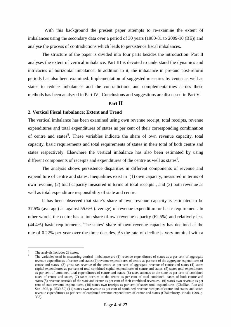
With this background the present paper attempts to re-examine the extent of
imbalances using the secondary data over a period of 30 years (1980-81 to 2009-10 (BE)) and
analyse the process of contradictions which leads to persistence fiscal imbalances.
The structure of the paper is divided into four parts besides the introduction. Part II
analyses the extent of vertical imbalance. Part III is devoted to understand the dynamics and
intricacies of horizontal imbalance. In addition to it, the imbalance in pre-and post-reform
periods has also been examined. Implementation of suggested measures by center as well as
states to reduce imbalances and the contradictions and complementarities across these
methods has been analyzed in Part IV. Conclusions and suggestions are discussed in Part V.
Part II
2. Vertical Fiscal Imbalance: Extent and Trend
The vertical imbalance has been examined using own revenue receipt, total receipts, revenue
expenditures and total expenditures of states as per cent of their corresponding combination
of centre and states8. These variables indicate the share of own revenue capacity, total
capacity, basic requirements and total requirements of states in their total of both centre and
states respectively. Elsewhere the vertical imbalance has also been estimated by using
different components of receipts and expenditures of the centre as well as states9.
The analysis shows persistence disparities in different components of revenue and
expenditure of centre and states. Inequalities exist in (1) own capacity, measured in terms of
own revenue, (2) total capacity measured in terms of total receipts , and (3) both revenue as
well as total expenditure responsibility of state and centre.
It has been observed that state‟s share of own revenue capacity is estimated to be
37.5% (average) as against 55.6% (average) of revenue expenditure or basic requirement. In
other words, the centre has a lion share of own revenue capacity (62.5%) and relatively less
(44.4%) basic requirements. The states‟ share of own revenue capacity has declined at the
rate of 0.22% per year over the three decades. As the rate of decline is very nominal with a
8 The analysis includes 28 states.
9 The variables used in measuring vertical imbalance are (1) revenue expenditures of states as a per cent of aggregate
revenue expenditures of centre and states (2) revenue expenditures of centre as per cent of the aggregate expenditures of
centre and states (3) gross tax revenue of the centre as per cent of aggregate revenue of centre and states (4) states
capital expenditures as per cent of total combined capital expenditures of centre and states, (5) states total expenditures
as per cent of combined total expenditures of centre and states, (6) taxes accrues to the state as per cent of combined
taxes of centre and states, (7) taxes accrues to the centre as per cent of total combined taxes of both centre and
states,(8) revenue accruals of the state and centre as per cent of their combined revenues. (9) states own revenue as per
cent of state revenue expenditures, (10) states own receipts as per cent of states total expenditures, (Chelliah, Rao and
Sen 1992, p. 2539-50) (11) states own revenue as per cent of combined revenue receipts of centre and states, and states
revenue expenditures as per cent of combined revenue expenditures of centre and states (Chakraborty, Pinaki 1998, p.
353).
Page 5 of 27
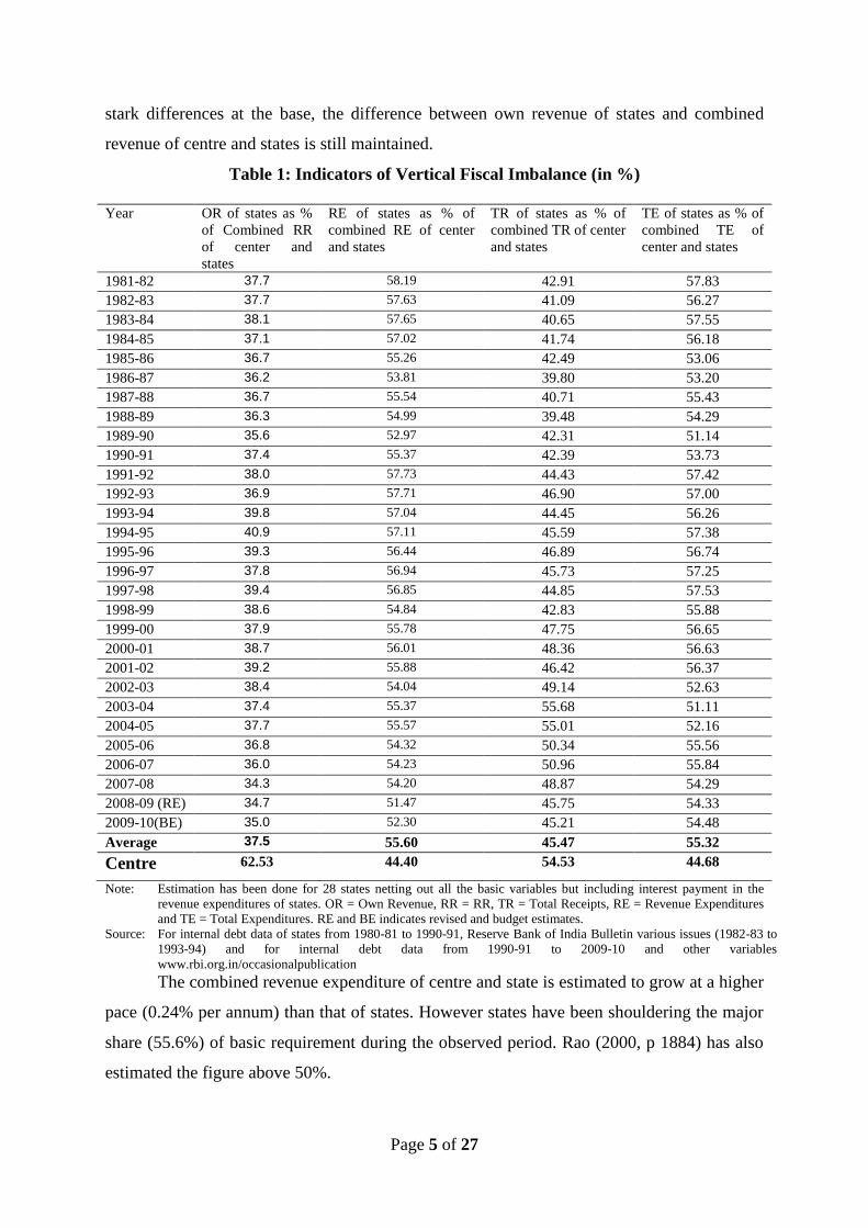
stark differences at the base, the difference between own revenue of states and combined
revenue of centre and states is still maintained.
Table 1: Indicators of Vertical Fiscal Imbalance (in %)
Year OR of states as %
of Combined RR
of center and
states
RE of states as % of
combined RE of center
and states
TR of states as % of
combined TR of center
and states
TE of states as % of
combined TE of
center and states
1981-82 37.7 58.19 42.91 57.83
1982-83 37.7 57.63 41.09 56.27
1983-84 38.1 57.65 40.65 57.55
1984-85 37.1 57.02 41.74 56.18
1985-86 36.7 55.26 42.49 53.06
1986-87 36.2 53.81 39.80 53.20
1987-88 36.7 55.54 40.71 55.43
1988-89 36.3 54.99 39.48 54.29
1989-90 35.6 52.97 42.31 51.14
1990-91 37.4 55.37 42.39 53.73
1991-92 38.0 57.73 44.43 57.42
1992-93 36.9 57.71 46.90 57.00
1993-94 39.8 57.04 44.45 56.26
1994-95 40.9 57.11 45.59 57.38
1995-96 39.3 56.44 46.89 56.74
1996-97 37.8 56.94 45.73 57.25
1997-98 39.4 56.85 44.85 57.53
1998-99 38.6 54.84 42.83 55.88
1999-00 37.9 55.78 47.75 56.65
2000-01 38.7 56.01 48.36 56.63
2001-02 39.2 55.88 46.42 56.37
2002-03 38.4 54.04 49.14 52.63
2003-04 37.4 55.37 55.68 51.11
2004-05 37.7 55.57 55.01 52.16
2005-06 36.8 54.32 50.34 55.56
2006-07 36.0 54.23 50.96 55.84
2007-08 34.3 54.20 48.87 54.29
2008-09 (RE) 34.7 51.47 45.75 54.33
2009-10(BE) 35.0 52.30 45.21 54.48
Average 37.5 55.60 45.47 55.32
Centre 62.53 44.40 54.53 44.68
Note: Estimation has been done for 28 states netting out all the basic variables but including interest payment in the
revenue expenditures of states. OR = Own Revenue, RR = RR, TR = Total Receipts, RE = Revenue Expenditures
and TE = Total Expenditures. RE and BE indicates revised and budget estimates.
Source: For internal debt data of states from 1980-81 to 1990-91, Reserve Bank of India Bulletin various issues (1982-83 to
1993-94) and for internal debt data from 1990-91 to 2009-10 and other variables
www.rbi.org.in/occasionalpublication
The combined revenue expenditure of centre and state is estimated to grow at a higher
pace (0.24% per annum) than that of states. However states have been shouldering the major
share (55.6%) of basic requirement during the observed period. Rao (2000, p 1884) has also
estimated the figure above 50%.

Page 6 of 27
The share of total capacity (total receipt) of states has been 45.5% whereas the total
requirement (total expenditure) share is found to be 55.3%. Even if the state share of total
capacity is growing marginally (0.97%) at a higher rate than that of the combined total
capacity, it is not able to influence the rate of growth of the ratio.
However the share of total requirement of states is increasing at a higher rate (1% per
annum) than the combined total requirement of centre and states, the trend of the ratio is
positive, indicating persistence increase in the expenditure of states.
Part III
3. Horizontal Fiscal Imbalance
Horizontal fiscal imbalance10
has been captured through two inter-related but different sets of
indicators, (1) components of receipts and expenditure, and (2) deficit indicators. In the first
set, the ratio of own revenue to revenue expenditure, own receipts to total expenditure, and
revenue expenditure to total expenditure of states have been used to understand the inequality
in own revenue capacity (ORC) to meet the basic needs, own total capacity to meet the
overall requirements, and the proportion of basic needs in total requirements respectively.
Similarly, the second set depicts inequality in deficits faced by states to meet different levels
of requirement. Elsewhere fiscal imbalance was also measured using components of receipts,
and expenditures11
.
Three important observations on the imbalance are (1) persistent inequality, (2)
growing inequality across states, and (3) further deepening up of inequality in the post-
liberalization period.
3.1: Deterioration in Fiscal Health of State
It is observed that the fiscal health of states has been deteriorated over time (see Table
2). States are on an average in a position to manage 60.5% of revenue requirements from
their own revenue sources which has been declining at an annual rate of 0.47% over 30 years.
As a result, no states are so far found self-sufficient as per the own revenue is concerned.
This implies declining tendency in fiscal health of states. The estimate reveals that the
average capacity varies from 37.6% (Bihar) to 82.6% (Haryana) indicating considerable level
of inequality. The inequality is estimated to be growing at 1.2% per annum pointing towards
widening disparity across states. One can observe a huge gap between the mean per capita
10
Here the analysis includes 14 major states. The population of 14 major states accounts for 95% of total population of
India (Raju, Swati 2012, p 77) and these states are to some extent similar in industrial units. 11 The horizontal imbalance has been measured through (1) own revenue as a per cent of total expenditure, (2) own
revenue as percentage of Net State Domestic Product (Mukhopadhyay et al 2003, pp 1417-19) (3) Own revenue as
percentage of GSDP, (4) Per capita GSDP, (5) per capita income and per capita own revenue, (6) per capita current
expenditures (7) percentage of own revenue to current expenditures (Rao 2004, p 54: Rao and Sen 1996, pp 106-7).
Page 7 of 27
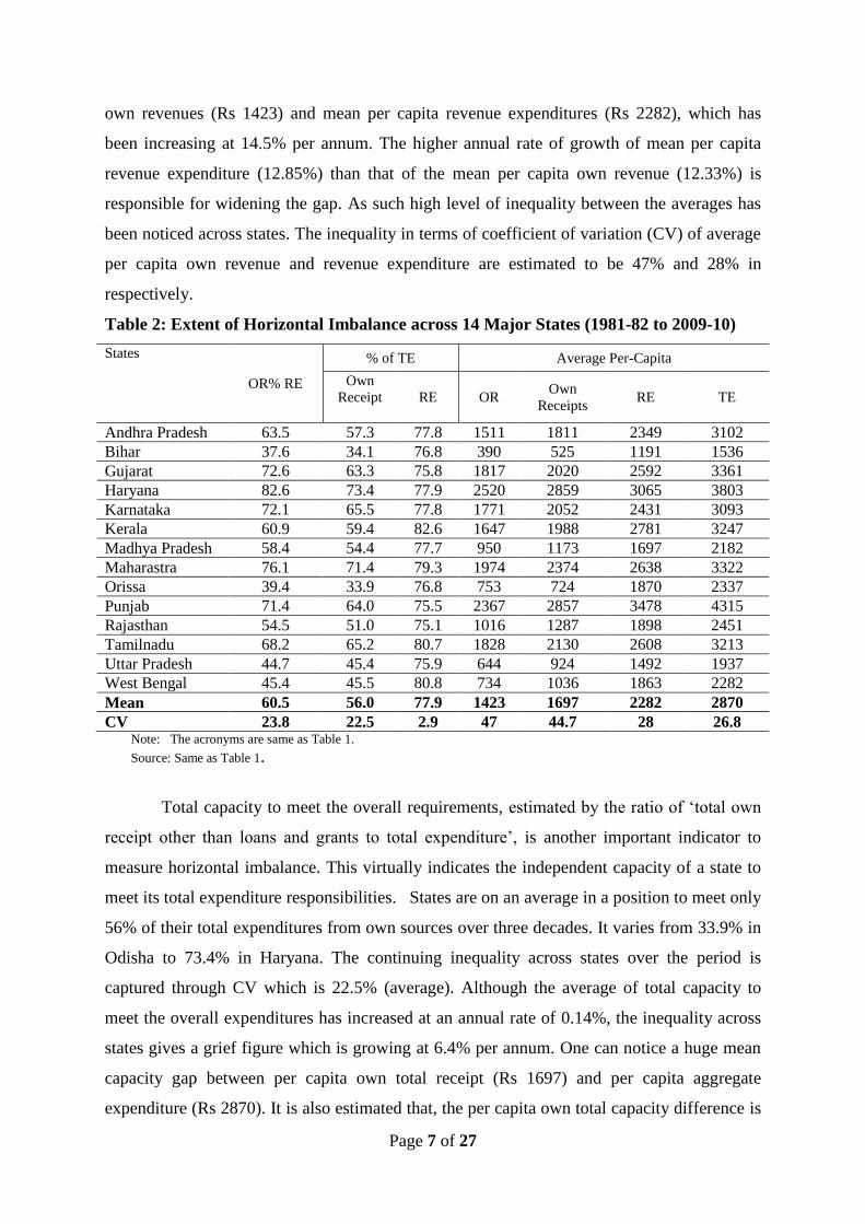
own revenues (Rs 1423) and mean per capita revenue expenditures (Rs 2282), which has
been increasing at 14.5% per annum. The higher annual rate of growth of mean per capita
revenue expenditure (12.85%) than that of the mean per capita own revenue (12.33%) is
responsible for widening the gap. As such high level of inequality between the averages has
been noticed across states. The inequality in terms of coefficient of variation (CV) of average
per capita own revenue and revenue expenditure are estimated to be 47% and 28% in
respectively.
Table 2: Extent of Horizontal Imbalance across 14 Major States (1981-82 to 2009-10)
States
OR% RE
% of TE Average Per-Capita
Own
Receipt
RE OR Own
Receipts RE TE
Andhra Pradesh 63.5 57.3 77.8 1511 1811 2349 3102
Bihar 37.6 34.1 76.8 390 525 1191 1536
Gujarat 72.6 63.3 75.8 1817 2020 2592 3361
Haryana 82.6 73.4 77.9 2520 2859 3065 3803
Karnataka 72.1 65.5 77.8 1771 2052 2431 3093
Kerala 60.9 59.4 82.6 1647 1988 2781 3247
Madhya Pradesh 58.4 54.4 77.7 950 1173 1697 2182
Maharastra 76.1 71.4 79.3 1974 2374 2638 3322
Orissa 39.4 33.9 76.8 753 724 1870 2337
Punjab 71.4 64.0 75.5 2367 2857 3478 4315
Rajasthan 54.5 51.0 75.1 1016 1287 1898 2451
Tamilnadu 68.2 65.2 80.7 1828 2130 2608 3213
Uttar Pradesh 44.7 45.4 75.9 644 924 1492 1937
West Bengal 45.4 45.5 80.8 734 1036 1863 2282
Mean 60.5 56.0 77.9 1423 1697 2282 2870
CV 23.8 22.5 2.9 47 44.7 28 26.8 Note: The acronyms are same as Table 1.
Source: Same as Table 1.
Total capacity to meet the overall requirements, estimated by the ratio of „total own
receipt other than loans and grants to total expenditure‟, is another important indicator to
measure horizontal imbalance. This virtually indicates the independent capacity of a state to
meet its total expenditure responsibilities. States are on an average in a position to meet only
56% of their total expenditures from own sources over three decades. It varies from 33.9% in
Odisha to 73.4% in Haryana. The continuing inequality across states over the period is
captured through CV which is 22.5% (average). Although the average of total capacity to
meet the overall expenditures has increased at an annual rate of 0.14%, the inequality across
states gives a grief figure which is growing at 6.4% per annum. One can notice a huge mean
capacity gap between per capita own total receipt (Rs 1697) and per capita aggregate
expenditure (Rs 2870). It is also estimated that, the per capita own total capacity difference is

Page 8 of 27
growing at the rate of 13.2% per annum. Besides, significant inequality has been observed
across states in per capita own total capacity (44.7 % CV) and per capita total expenditure
requirements (26.8% CV).
Insignificant inequality (2.9% CV) across states in the proportion of revenue
expenditures to total expenditures was noticed because of marginal difference between
numerator and denominator variables maintained by states. However, a stark inequality was
estimated (high CV) across states while considering both variables separately. It is estimated
that in three decades the average ratio of both variables is more or less 78% implying more
than two third of the total expenditure is spent for basic needs by states. It is highest in Kerala
with 82.6% and lowest in Rajasthan with 75.1%. As mentioned earlier, the inequality across
states in per capita revenue expenditure (28% CV) and per capita total expenditure (26.8%
CV) found significant.
3.2 Inequality under Dis-aggregation:
The disaggregated analysis across different income group states shows widening inequality12
.
Inequality in ORC to meet the basic needs measured in terms of CV found very high across
LIGS (19.5%) followed by MIGS (16.5%) and HIGS (6.7%). It is estimated that on an
average LIGS are in a position to manage around 50% of their basic needs from ORC, which
is 62% and 75% among the MIGS and HIGS respectively. ORC to meet the basic needs has
been declining at an annual rate of 0.52%, 0.23% and 0.54% for HIGS, MIGS and LIGS
respectively. In addition to it, the inequality across the HIGS increased at the rate of 26.3%
per annum followed by MIGS (6.3%) and LIGS (3.1%). Decrease in ORC to meet basic
needs and increasing inter and intra group inequality clearly speaks about the frustrating
economic instability.
It is interesting to note that there are significant imbalances observed in the per capita
capacity as well as needs across three income groups states. The three decades averages per
capita ORC for HIGS is nearly 2.6 times higher than that of the LIGS. Similarly, the per
capita expenditure inequality found to be growing at the rate of 14.1%, 6.2% and 7.8% per
annum for HIGS, MIGS and LIGS respectively. The inequality in own revenue and
expenditure remains intact among these groups as the rate of growth in per capita ORC is
more or less same (around 12% per annum), so also the per capita expenditure (12.8 to 13%
per annum).
12 The states have been divided into High Income Group States (HIGS), Middle Income Group States (MIGS) and Low
Income Group States (LIGS). Mean per capita NSDP of 14 major states over 30 years has been taken as a dividing line
for LIGS. States such as Bihar, Orissa, UP, MP and Rajasthan, fall under this category. The combined mean of the
mean per capita income of states except LIGS has been used to divide states into HIGS and MIGS.

Page 9 of 27
3.3 Imbalances after liberalization:
Improvement in the quality of infrastructure is one of the prerequisites to accelerate the
growth process (Rao 2002, p 3261). The market-based reform generates more inequality
when there is unequal capacity among states for infrastructure development. There are
evidences of divergences in growth performances among states because of unequal capacity
for infrastructure in the post reform era (Ahluwalia 2000). The major challenge faced by
poorer states in the post reform period is to chase competitive infrastructure investment in
order to attract foreign capital investment. States with infrastructure or capacity to invest on
infrastructure perform well; whereas, others found struggling even to meet the basic needs.
With this backdrop, this part will explore the imbalances in pre and post-liberalization
periods.
The ORC to meet the basic needs has gone down from 64.2% in pre-liberalization to
58.4% in post liberalization period. The inequality captured through CV across states after
economic reforms has increased from 20.7% to 26% (see Table 3). Capacity and inequality
among different income group states shows the same trend, even though the per capita own
revenue as well as revenue expenditure has considerably increased during post reform period.
This also complemented with higher inequality across states during post reform period.
The proportion of own total receipt to total expenditure has increased from 54.9% in
pre-reform period to 56.9% in post reform period. When the average of own receipt reported
8.64, the average of total expenditure reported 8.37 fold jump from pre-to post-reform period.
The relatively higher jump in the earlier variable than the later variable makes the proportion
unequal. Inequality has widened in the post reform by 5% more than the pre reform period.
The share of revenue expenditure in total expenditures has increased from 73% during pre-
refom to 81% during post-reform period. The rise was around 10% and 9% for HIGS and
LIGS, whereas it is 4% for the MIGS, indicating less scope for capital investment in former
two groups.
Table 3: Horizontal Fiscal Imbalance (14 Major States) in Pre and Post Liberalization
Pre- Liberalization Post- Liberalization
Mean CV Mean CV
% of OR to RE 64.2 20.7 58.4 26
% Own total Receipts to TE 54.5 19.6 56.9 24.6
% of RE to TE 72.9 5.8 80.8 2.9
% of Capital Expenditure to TE 27.2 15.6 19.2 12.3
Note: The acronyms are same as Table 1.
Source: Same as Table 1.

Page 10 of 27
3.4 Deficit Indicators: What do they speak about?
Wide variation in the deterioration in fiscal situation of states estimated with the help of
deficit indicators has been widely discussed in literature (Rao 2002, p 3263).
Per capita RD, FD and PD of sample states have been growing at 27.05, 11.53 and
61.85 % respectively (figure 1)13
indicating financial deterioration of states during the
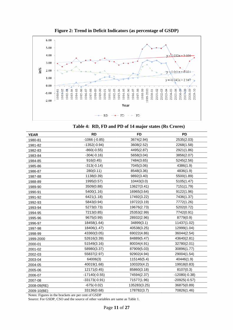
observed period. While the proportions of RD and FD as a percentage of the GSDP shows
positive slopes, PD as percentage of GSDP gives a reverse trend indicates lower rate of
growth of PD than that of GSDP (figure 2 & Table 4). Rao (2002, p 3262; 2003, p 53 and
2004, p 1821) has also observed the increasing trend of RD, FD and PD as a percentage of
GDP during 1980-81 to 2001-02. However, a declining trend has been observed in the PD
from 2003-04 to 2007-08 that further took a positive slope after 2007-08. Declining trend in
PD may be observed due to the higher rate of growth of interest payment than that of the FD.
Elsewhere, it has also been mentioned that deterioration in the state finances is due to the rise
in the percentage of interest payment over the years (Rao 2000, p 54).
Figure 1: Per Capita Deficit Indicators of States (in average)
13 While RD indicates the inability to meet the basic needs, the efforts for basic needs as well as further investment is
captured by FD. In other words, accumulation of public debt, interest payment and RD constitutes the major
components of FD (Rakshit 2005, p 3440). Closer the RD to FD, lesser is the scope for further growth which in turn
accelerates debt burden in the form of PD. The growth rate of deficits has been estimated from deficits year‟s figures of
sample states. Even though few states have shown surplus figures in few years, the present estimation excluded these
years as the objective here is to estimates the trend of deficit. It is worthy to note that, in case of PD and FD most of the
states have deficit figures with few exceptions. However, RD figures of sample states are a mix-up of both surplus and
deficits.
Page 11 of 27
Figure 2: Trend in Deficit Indicators (as percentage of GSDP)
Table 4: RD, FD and PD of 14 major states (Rs Crores)
YEAR RD FD PD
1980-81 -1066 (-0.85) 3674(2.94) 2535(2.03)
1981-82 -1352(-0.94) 3608(2.52) 2268(1.58)
1982-83 -860(-0.55) 4495(2.87) 2921(1.86)
1983-84 -304(-0.16) 5658(3.04) 3856(2.07)
1984-85 916(0.45) 7484(3.65) 5245(2.56)
1985-86 -313(-0.14) 7045(3.06) 4386(1.9)
1986-87 280(0.11) 8548(3.36) 4836(1.9)
1987-88 1138(0.39) 9892(3.40) 5500(1.89)
1988-89 1995(0.57) 10443(3.0) 5105(1.47)
1989-90 3509(0.88) 13627(3.41) 7151(1.79)
1990-91 5400(1.16) 16965(3.64) 9122(1.96)
1991-92 6421(1.18) 17492(3.22) 7436(1.37)
1992-93 5843(0.94) 19722(3.19) 7772(1.26)
1993-94 5273(0.73) 19676(2.73) 5202(0.72)
1994-95 7213(0.85) 25353(2.99) 7742(0.91)
1995-96 9675(0.99) 28932(2.96) 8779(0.9)
1996-97 18458(1.64) 34899(3.1) 11437(1.02)
1997-98 18406(1.47) 40538(3.25) 12999(1.04)
1998-99 43360(3.05) 69022(4.86) 36044(2.54)
1999-2000 52616(3.39) 84889(5.47) 43640(2.81)
2000-01 51549(3.16) 80034(4.91) 32780(2.01)
2001-02 58980(3.37) 87909(5.03) 30896(1.77)
2002-03 55837(2.97) 92902(4.94) 29004(1.54)
2003-04 64006(3) 115146(5.4) 40446(1.9)
2004-05 40019(1.68) 100320(4.2) 19918(0.83)
2005-06 12171(0.45) 85860(3.18) 8107(0.3)
2006-07 -17140(-0.55) 74594(2.37) -12080(-0.38)
2007-08 -33173(-0.91) 71577(1.96) -20925(-0.57)
2008-09(RE) -675(-0.02) 135283(3.25) 36875(0.89)
2009-10(BE) 33136(0.68) 178782(3.7) 70826(1.46)
Notes: Figures in the brackets are per cent of GSDP Source: For GSDP, CSO and the source of other variables are same as Table 1.

Page 12 of 27
States were in a position to go for further capital investment covering revenue
expenditure responsibility from own revenue sources till 1985-86. However the scope of
capital investment was reduced when RD showed positive trend during 1986-87 to 2003-04.
This in turn led to further rise in RD. The increasing trend in RD accentuated with the
implementation of 5th
pay commission in 1997-98 (Rao 2003 p.53, Rao 2002 p 3262).The per
cent of RD to FD (quality of deficit) has increased from 12% in 1987-88 to 67% in 2001-02
with the implementation of the recommendations of fifth pay commission. In the same line
FD as per centage of GSDP, being influenced by the trend of RD due to their natural
relationship, has increased (2.5% per annum) during the same period. RD decline after 2003-
04 continuously generating revenue surplus and reducing FD with the hope of getting the
conditional benefit of MTFRP.
The rate of growth of PD as a percentage of GSDP has been increasing at 11.8% per
annum in three decades, indicating acceleration in outstanding loan. The increasing deficits
both in per capita as well as ratio of GSDP clearly speaks about the increasing gap burden to
meet different levels of need. The accumulation of loan has an adverse impact on capital
formation (Lalvani, Mala 2009, p 59) as well as compels states either (1) to reduce the
expenditure on social and economic service (Rao and Sen 1996; Varghese 2006) or (2) to
increase the revenue deficit. It certainly leads to the deterioration in the fiscal health of states
(Rao 2004, p 1821).
Five inferences can be drawn from the analysis of deficit indicators, (1) debt burden is
mounting, (2) No scope for expansion in social and economic service, (3) no scope for capital
investment, (4) there is stark inequality among states and (5) the process of devolution of
revenue is ineffective.
Part IV
4. The Paradox of Fiscal Imbalances
The observed persistence rising fiscal imbalances in India is a bi-product of policy
paradox. Efforts to reduce these imbalances work like a boomerang against the principles of
fiscal federalism. Complementarities among methodologies having same objectives and
contradictions among methodologies with different objectives adopted by UFC and PC
accelerate the pace of imbalances. In other words, methodologies adopted to maintain equity
complements with each other. Similarly methodologies used to maintain efficiency also
complements each other. However, methodologies adopted to maintain equity contradicts
with methodology used to increase efficiency (See Table 8).
Page 13 of 27
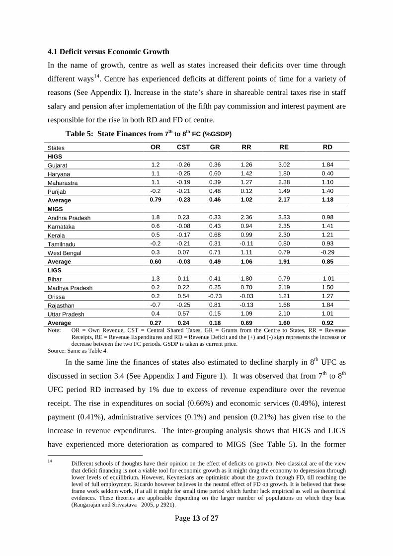
4.1 Deficit versus Economic Growth
In the name of growth, centre as well as states increased their deficits over time through
different ways14
. Centre has experienced deficits at different points of time for a variety of
reasons (See Appendix I). Increase in the state‟s share in shareable central taxes rise in staff
salary and pension after implementation of the fifth pay commission and interest payment are
responsible for the rise in both RD and FD of centre.
Table 5: State Finances from 7th
to 8th
FC (%GSDP)
States OR CST GR RR RE RD
HIGS
Gujarat 1.2 -0.26 0.36 1.26 3.02 1.84
Haryana 1.1 -0.25 0.60 1.42 1.80 0.40
Maharastra 1.1 -0.19 0.39 1.27 2.38 1.10
Punjab -0.2 -0.21 0.48 0.12 1.49 1.40
Average 0.79 -0.23 0.46 1.02 2.17 1.18
MIGS
Andhra Pradesh 1.8 0.23 0.33 2.36 3.33 0.98
Karnataka 0.6 -0.08 0.43 0.94 2.35 1.41
Kerala 0.5 -0.17 0.68 0.99 2.30 1.21
Tamilnadu -0.2 -0.21 0.31 -0.11 0.80 0.93
West Bengal 0.3 0.07 0.71 1.11 0.79 -0.29
Average 0.60 -0.03 0.49 1.06 1.91 0.85
LIGS
Bihar 1.3 0.11 0.41 1.80 0.79 -1.01
Madhya Pradesh 0.2 0.22 0.25 0.70 2.19 1.50
Orissa 0.2 0.54 -0.73 -0.03 1.21 1.27
Rajasthan -0.7 -0.25 0.81 -0.13 1.68 1.84
Uttar Pradesh 0.4 0.57 0.15 1.09 2.10 1.01
Average 0.27 0.24 0.18 0.69 1.60 0.92
Note: OR = Own Revenue, CST = Central Shared Taxes, GR = Grants from the Centre to States, RR = Revenue
Receipts, RE = Revenue Expenditures and RD = Revenue Deficit and the (+) and (-) sign represents the increase or
decrease between the two FC periods. GSDP is taken as current price.
Source: Same as Table 4.
In the same line the finances of states also estimated to decline sharply in 8th
UFC as
discussed in section 3.4 (See Appendix I and Figure 1). It was observed that from 7th
to 8th
UFC period RD increased by 1% due to excess of revenue expenditure over the revenue
receipt. The rise in expenditures on social (0.66%) and economic services (0.49%), interest
payment (0.41%), administrative services (0.1%) and pension (0.21%) has given rise to the
increase in revenue expenditures. The inter-grouping analysis shows that HIGS and LIGS
have experienced more deterioration as compared to MIGS (See Table 5). In the former
14
Different schools of thoughts have their opinion on the effect of deficits on growth. Neo classical are of the view
that deficit financing is not a viable tool for economic growth as it might drag the economy to depression through
lower levels of equilibrium. However, Keynesians are optimistic about the growth through FD, till reaching the
level of full employment. Ricardo however believes in the neutral effect of FD on growth. It is believed that these
frame work seldom work, if at all it might for small time period which further lack empirical as well as theoretical
evidences. These theories are applicable depending on the larger number of populations on which they base
(Rangarajan and Srivastava 2005, p 2921).

Page 14 of 27
groups of state deterioration increased by 1.2% and 0.92% from 7th
to 8th
UFC respectively
due to more than 2 folds rise in revenue expenditures than revenue receipt (RR). The rise in
revenue expenditure of HIGS is because of the rise in expenditures on social (0.88%) and
economic services (0.31%), interest payment (0.48%), administrative services (0.13%) and
pension (0.25%) and decline in central shared taxes (0.23%). Similarly the rise in revenue
expenditure of LIGS are due to the rise in expenditure on social (0.33%) and economic
services (0.75%), interest payment (0.4%), administrative services (0.1 %) and pension
(0.14%).
Keeping in view the declining financial situation, the central government directed states
during 9th-2
FC to control RD as well as FD and increase capital investment through remedial
measures. However, the finances of states instead of improving deteriorated sharply due to
lack of remedial measures. The share of revenue expenditures of states increased 4 times of
RR from 8th
to 9th-2
FC leading to increase in RD (0.7%). It is because of rise in interest
payment (0.54%), pension (0.11%) and miscellaneous general economic services (0.37 %)
and constant central shared taxes and grants and marginal rise (0.1%) in own revenue of
states. The inter grouping state estimation reflects that the deterioration is more in LIGS.
However it is relatively more in HIGS and MIGS than LIGS (see Table 6). The revenue
expenditures increased by 0.6% and 0.1% and RR declined by- 0.1% and -0.5% in HIGS and
MIGS respectively. The own tax laxity as well as the decline in central shared taxes and
grants has contributed in reducing the RR.
The RD of all states (average) increased by 1.2% between 9th
to 10th
UFC due to
decline in the RR (-1.3%) given the same level of revenue expenditures. The decline in the
share of central shared taxes (-0.1%) due to reduction in tax-GDP ratio of the centre, and
grants (-0.7%) to states as well as the own revenue (-0.5%) due to decline in the tax effort and
tax exemption to attract new investment has led to reduction in RR. The increase in the
interest payment due to mounting of borrowing and rise in salary and pension with the
implementation of fifth pay commission have given rise to the constancy in revenue
expenditures (Kurian 2005, p 3429; Ghosh 2005, p 3436). It is further observed that the
deterioration is more in HIGS and LIGS than MIGS (See Table 7). RD increased due to
decline in RR (0.9%) as well as rise in revenue expenditure (0.2%) in HIGS. The significant
decline in own revenue (0.6%) as well as marginal fall in central shared taxes (0.1 %) and
grants (0.2%) has been responsible for the fall in RR. The increase in interest payment (0.5%)
and pension (0.3%) over the reduction of social and economic expenditures (0.6%) has led to
rise in revenue expenditures. In LIGS the RD increased due to significant decline in RR (-

Page 15 of 27
1.6%) and rise in revenue expenditure (0.1%). The reduction of own revenue (-0.4%) and
grants (-1.1%) has reduced the RR.
Table 6: State Finances from 8th
to 9th-2
FC (%GSDP)
States OR CST GR RR RE RD
HIGS
Gujarat 0.5 -0.29 -0.50 -0.25 -0.13 0.05
Haryana 1.7 -0.03 -0.68 0.99 2.10 1.11
Maharastra -1.4 -0.29 -0.21 -1.94 -2.15 -0.21
Punjab 1.1 -0.04 -0.28 0.77 2.49 1.72
Average 0.5 -0.2 -0.4 -0.1 0.6 0.7
MIGS
Andhra Pradesh -1.9 -0.37 -0.03 -2.32 -2.36 -0.05
Karnataka -0.2 -0.21 -0.10 -0.54 -0.65 -0.11
Kerala -0.1 0.02 -0.05 -0.17 0.24 0.52
Tamilnadu 0.5 -0.11 -0.06 0.30 2.31 2.01
West Bengal 0.0 0.16 -0.02 0.17 1.10 0.92
Average -0.4 -0.1 -0.1 -0.5 0.1 0.7
LIGS
Bihar -0.3 0.18 0.61 0.48 4.11 3.03
Madhya Pradesh -0.2 -0.19 0.33 -0.11 0.19 0.30
Orissa 0.7 1.09 0.51 2.33 2.60 0.28
Rajasthan 0.4 0.25 -0.04 0.65 -0.12 -0.78
Uttar Pradesh 0.4 -0.08 0.75 1.10 2.26 1.19
Average 0.2 0.2 0.4 0.9 1.8 0.8
Note: Same as Table 5.
Source: Same as Table 4.
Table 7: State Finances from 9th-2
to 10th
FC (%GSDP)
States OR ST GR RR RE RD
HIGS
Gujarat -0.8 0.11 -0.24 -0.96 -0.16 0.80
Haryana -0.4 -0.08 -0.08 -0.61 1.21 1.82
Maharastra -0.9 -0.31 -0.38 -1.61 -0.60 1.00
Punjab -0.1 -0.13 -0.27 -0.55 0.21 0.76
Average -0.6 -0.1 -0.2 -0.9 0.2 1.1
MIGS
Andhra Pradesh -0.9 0.03 -0.44 -1.28 0.04 1.32
Karnataka -0.5 0.02 -0.40 -0.88 -0.26 0.62
Kerala 0.1 -0.22 -0.69 -0.82 0.21 1.03
Tamilnadu -0.5 -0.46 -0.59 -1.55 -1.91 -0.36
West Bengal -1.0 -0.23 -0.56 -1.80 0.06 1.86
Average -0.6 -0.2 -0.5 -1.3 -0.4 0.9
LIGS
Bihar -0.5 0.60 -1.05 -0.92 -0.90 -0.08
Madhya Pradesh 0.0 0.15 -0.72 -0.62 0.92 1.53
Orissa -0.6 -0.74 -1.13 -2.47 0.43 2.90
Rajasthan -0.6 -0.40 -1.33 -2.29 -0.16 2.13
Uttar Pradesh -0.5 0.30 -1.52 -1.71 0.03 1.74
Average -0.4 0.0 -1.1 -1.6 0.1 1.6
Note: Same as Table 5.
Source: Same as Table 4.

Page 16 of 27
MTFRP was introduced to bring improvement in the fiscal health of states during 11th
FC period (See Table 8). It was also supplemented by tax effort and fiscal discipline criterion
with the weightage of 5% and 7.5% respectively15
. The inter-grouping estimation shows that
RD is more in HIGS and MIGS than LIGS (see Appendix II). It is also observed from intra
grouping estimation that even if there is reduction of RD in Haryana, Tamilnadu, MP and
Odisha and marginal increase in RD has been observed in other LIGS. However, high
deficits are found in rest of HIGS and MIGS.
In Haryana the reduction in RD (1.25%) is due to higher (-1.3%) decline in revenue
expenditures than the RR. The shares of own revenue, central shared taxes and grants have
declined by -1.7%, -0.4% and -0.1% respectively from 10th
to 11th
FC period while revenue
expenditures by -3.5% of GSDP. Tamilnadu experienced marginal (-0.06%) fall in RD due to
marginal rise (0.05%) in RR over revenue expenditure despite the decline in central shared
taxes (-0.2%). It has been estimated that in Tamilnadu the own revenue and grants have
increased by 1 and 0.15% respectively. It has been observed that the share of central shared
taxes in both Haryana and Tamilnadu has declined due to rise in the weightage (2.5%) of
income distance method used in the distribution of such taxes than the previous commission.
In Odisha RR has increased 2.43% more than revenue expenditures leading to 0.6%
decline in RD. The own revenue, central shared taxes and grants have increased by 1.5%,
1.2% and 0.13% respectively while the revenue expenditures has increased by 0.4%.
Similarly 0.23% decline in RD has been observed in MP. It is because the RR has marginally
(0.27%) increased over revenue expenditures. In all other LIGS the revenue expenditures
have increased more than the own revenue. But due to greater weightage assigned to the
income distance criterion the share of central shared taxes of these states has increased
leading to low RD.
However, increased deficits have been observed in all other HIGS and MIGS. The
deficits increased to a greater extent in Gujarat, Maharastra, Punjab of HIGS, Kerala and
West Bengal of MIGS. In Gujarat the revenue expenditures have increased 1.98% more than
the RR leading to rise in RD. The own revenue and grants have marginally (0.1% and 0.58%
respectively) increased along with fall in central shared taxes by -0.35%. The own revenue of
Gujarat has observed to be constant due to the tax exemptions and subsidy offered by the
state. Otherwise it could have registered a growth during this period. In addition to that,
15 The increase in tax effort and fiscal discipline measured in terms of improvement in own revenue as per cent of
total revenue expenditures increases the share of state in central shared taxes and vice versa which in turn helps in
reducing or increasing the RD respectively.

Page 17 of 27
higher weightage of income distance criterion led to the reduction of central shared taxes.
However the revenue expenditures have increased by 2.3% leading to 1.98% rise in RD. The
revenue expenditures have increased 1.61% more than the RR in Maharashtra which leading
to rise in deficits by 1.63%. Although the own revenue has increased marginally (0.7%) the
decline in central shared taxes (-0.18%) and grants (-0.04%) as well as the rise in the revenue
expenditures (2.1%) have increased the deficits.
In Punjab the revenue expenditures have increased 1.21% more than the RR. Although
the own revenue and grants have increased by 1.9% and 0.08% respectively, the central
shared taxes have declined by -0.19% and revenue expenditures have increased by 3%. Thus
the RD increased by one percentage.
Among the MIGS highest RD have been observed in Kerala and West Bengal. In
Kerala the deficit has increased by 1.35% due to increase in revenue expenditure (1.2%) over
the revenue receipt (0.18%). marginal rise (0.1%) in own revenue, declining central shared
taxes (0.24%) and grants (0.04%) and increased revenue expenditures (1.2%). Increased RD
of 1.56 % has been observed in West Bengal due to 1.53% excess increase in revenue
expenditures over the RR. However, marginal rise in deficits have been found in AP and
Karnataka.
When FRBMA during 12th
UFC along with the increased weightage of tax effort (7.5%)
and fiscal discipline (7.5%) criterion in the distribution of central shared taxes more
contraction in RD was seen in LIGS and HIGS and MIGH (see Appendix III). All states
introduced FRBMA, but targets were not achieved by HIGS and MIGS (See Appendix III).
Specifically Punjab, Kerala and West Bengal did not fulfill the targets. Although RD has
reduced by 1.83% in Punjab the decline in own revenue (-0.4%) has not enabled the state to
eliminate the RD even if the central shared taxes and grants have increased by 0.45% and
0.78% respectively. In all other HIGS even if there has been marginal decline in the own
revenue from 11th
FC to 12th
FC the significant decline in revenue expenditures has enabled
them to eliminate deficit and generate revenue surpluses.
In Kerala RD has reduced by 1.92% due to rise in central shared taxes and grants by
0.24 and 0.43% respectively and fall in revenue expenditures (1.2%). The own revenue has
remained constant. If the own revenue had increased the RD could have been eliminated.
Similarly in West Bengal, RD could not be removed due to its high level even if there has
been marginal rise (1.2 %) in RR and decline (0.3%) in revenue expenditures. The RR have
increased due to increase in own revenue, central shared taxes and grants by 0.4%, 0.48% and

Page 18 of 27
0.33% respectively. The revenue surpluses have been generated in all other MIGS due to
significant rise in own revenue and fall in revenue expenditures.
In all LIGS the RR have increased over revenue expenditures due to rise in own
revenue as well as central shared taxes and grants so that they have been enabled to generate
revenue surpluses eliminating the revenue deficits. It has been estimated that the rise in
central shared taxes and grants is greater than that of the own revenue in all states. However,
Bihar, UP and Rajasthan has not been able to meet the target of FD due to excessive FD in
previous FC period.
4.2 Contradicting Methodologies and Fiscal Imbalances
The persistence increased deficits across HIGS and MIGS over different FC periods
reflects two sets of inferences. The first set of inferences derived from state finances from 7th
to 11th
FC periods includes increased revenue expenditures and grants as well as declining
share of central shared taxes and own revenue. The second set of inferences derived from the
state finances during 12th
FC period is declining revenue expenditures, marginal rise in own
revenue as well as the share of central shared taxes and grants.
From the first set of inferences it seems that states have increased (1) the gap between
non plan revenue expenditure and the sum of own revenue and central share taxes to get more
gap grant, (2) revenue expenditure financed through more loan to get more grant from PC,
(3) the proportion of interest payment which is a components of revenue expenditure raising
loan to avail more gap grants and grant from PC, and (4) the equity principle have increased
the gap between non plan revenue expenditure and the sum of shared tax and own revenue of
HIGS and MIGS. As a result grants to these states have increased.
Thus it is cleared that deficits are the result of complementarities of gap filling approach
(GFA) and equity principle of FC and Gadgil formula of PC16
(see Table 8). According to the
GFA the rise or fall in gap grants depends on expansion and contraction of the gap between
non plan revenue expenditure and sum of central shared taxed and own revenue of states,
which in turn depends on the tax effort of states, the weightage assigned to equity and fiscal
discipline criterion, the proportion of loans as well as non- plan revenue expenditures on
general, social and economic services. There is direct relationship between the gap and the
second, fourth and fifth variables on the part of the HIGS and MIGS17
. There is indirect
16 Initially (first three finance commission period) the gap grants were given to states on the basis of
difference between the sum of central share taxes and own revenue of states as well as revenue
expenditure. 17 However, the relationship between the gap and the weightage assigned to equity criterion is indirect in case of
LIGS.

Page 19 of 27
relationship between the gap and the first and third variable on the part of the HIGS and
MIGS. The GFA pursues either tax laxity18
or increasing non-plan revenue expenditures or
both to all states while the EP with increasing weights reduces the share of better off states
from central shared taxes which help to get more gap grants19
. Elsewhere it has been
mentioned that GFA encourages tax laxity and wasteful expenditures (Rao and Sen 1996, p
147: Rao and Chelliah 1996, p 25).
The GF of PC encourages borrowing of states from the centre to avail more grants
because grant rooted through this formula are determined by the proportion of loan by the
states20
. It supplements states to reap the implicit benefit of increased non-plan revenue
expenditures as well as tax laxity through GFA. Due to less possibility of positive gap in the
later formula in HIGS and MIGS and increasing weightage of equity principle in the
distribution of central shared taxes (See success of states section of GFA of the Table 8),
these states tried to take benefits through GF21
raising the non-plan unproductive
expenditures (interest payments and pensions) increasing loans and decreasing own revenue.
Thus the increasing gap under GFA complements GF to raise the proportion of loan. The
increased loans being spend on the plan revenue expenditures produced no return leading to
RD and increased FD (borrowing outstanding loans and interest payment). It has been argued
that the steady financial deterioration of states is due to accumulation of state debts (Kannan
et al 2004, p 480). When MTFRP was introduced along with 12.5% weightage of fiscal
discipline criteria during 11th
FC to restructure the state finances, deficit could not be
reduced. It seems that state might have compared the benefits of these programmes with
combined benefits of GFA, EP and GF since the former contradicts with the later and bypass
the former due to its small size (see Table 8 column-10 row-6). Elsewhere it is argued that
because the size of the cake under MTFRP is small (2% total transfers) general category
states bypass the benefits ought to be received through MTFRP (Rao 2004 p. 1823).
18 The tax laxity occurs in the form of tax exemption and absence of control on tax evasion and avoidance. 19 The weight of income distance method and inverse income method used as equity principle has increased from 25
per cent since 7th FC period to 62.5 per cent in 11th FC and further declined to 50 per cent in 12th FC. These
methods reduce the share of HIGS and MIGS on central share taxes due to negative relationship between fiscal
capacity and the share of these taxes of state. 20 Although there have been minor modifications in the GF, the basic structure remains the same. 21 With continuous increase in the share of states on central shared taxes over different UFCs and higher own
revenue in the HIGS and MIGS the post devolution gap has declined.

Page 20 of 27
Table 8: Contradicting Formulae
Formulae Time FC Objective Conditions CoMF CoNF Process of Contradiction SS FS
GFA
1952-
53 to 2014-
15
1st-13th
Maintain
horizontal
balance
Non-Plan Tax revenue account deficit
(1) MTFRP
(2)
FRBMA (3) FDC
GFA: The objective behind GPA is to devolve as per the
deficiency in fiscal capacity (Non-Plan revenue account
gap) of states. This gap grants induces states to lax in own revenue generation and increase revenue expenditure on
the maintenance of socio economic services and interest
payment. This nature of fiscal deficiency calls for rise in loan which further accelerate deficits (RD and FD). On
the other hand the conditions of MTFRP, FRBM and FD
encourages to bring improvement in own revenue and reduction in revenue expenditure (both plan and non-plan)
results in reduction in deficits.
Odisha, WB and
Rajasthan (7th
FC) (Rao and Chelliah, 1996, p.
26; Rao and Sen,
1996, p. 147)
All major states
except
Odisha, WB and Rajasthan
(7th FC) (Rao and
Chelliah, 1996, p. 26;
Rao and Sen,
1996, p. 147)
GF
1969-
70 to
2014-
15
5th -
13th
Maintain
horizontal balance
(1) 1:0.42 loans and grants ratio for
general category states
(2) 1: 9 loans and grants ratio
for special category states
GFA
(1)
MTFRP
(2) FRBMA
(3) FDC
GF: Gadgil formula is a combination of Population criterion, equity principle, Fiscal discipline, and Special
problem. As per the norm of Gadgil formula, higher the
loan higher will be the loan (Rs 0.42 and Rs 9 of grants for every rupees of loan to general and special categories
state respectively). In other words, it encourages states
increase in borrowing. Since borrowing is directly
compensated by the central government through GF, it
encourages states not to rethink about revenue generation
through increase in tax effort and expansion of tax base. This fortunately complemented by the conditions of GFA.
On the other hand the conditions of MTFRP, FRBM and FD encourages to bring improvement in own revenue and
reduction in revenue expenditure (both plan and non-plan)
results in reduction in deficits.
HIGS (Rao and
Sen, 1996, p. 151)
MIGS (Rao and
Sen, 1996, p. 151)
EP
Maintain
horizontal balance
GFA
(HIGS &MIGS)
(1)
MTFRP
(2) FRBMA
(3) FDC
EP: The EP argues for progressive distribution of share
taxes. As a result the high income group states gets less as
compared to the middle and low income group state. Here
the High income group states in order to avail the benefits
of GFA, increases the gap between revenue and
expenditure by either (1) tax lexity, or (2) increase in non plan revenue expenditure, or (3) both. This contradicts
with the fundamentals of MTFRP, FRBM and FD.
LIGS MIGS and HIGS
FDC
Increase
efficiency
among states
(1) MTFRP
(2)
FRBMA
(1) GFA
(2) GF
(3) EP
FDC tries to reduce deficits but GFA, GF and EP encourage deficits
MTFRP 2000-
01 to
2004-
11th
To increase
efficiency
among states
(1) Zero RD
(2) GFD to 2.5% of GSDP
(3) IP to be less than 18-
FDC
(1) GFA
(2) GF
(3) EP
MTFRP tries to reduce deficits but GFA, GF and EP
encourage deficits thereby inefficiency.
Special Category
States (Rao,
2004, p. 1823)
General Category
States
(Rao, 2004, p.

Page 21 of 27
05 20% of RR
(4) Wages and Salaries less than 5% of the
increase in CPI
(5) increase in IP not be more than 10% per year
(6) Explicit subsidies to be
50% over five year period
1823)
FRBMA
2005-
06 to
2009-10
12th To bring fiscal discipline
among states
(1) Zero RD by 2008-09 (2) FD to 3% of GSDP/
ratio of IP to RR
(3) Annual targets for RD and FD
(4) Annual statements on
prospects for the state economy and related fiscal
strategy
(5) special statements of budget giving in detail the
number of employees in
government, public sector, aided institutions and
related salaries
FDC (1) GFA (2) GF
(3) EP
FRBMA tries to reduce deficits but GFA, GF and EP
encourage deficits thereby inefficiency.
Goa, Punjab, Haryana,
Maharastra,
Kerala, Gujarat, Tamilnadu,
Karnataka, AP
and WB (Rao and Jena, 2005, p.
3409)
Rajasthan,
Chhatisgarh,
MP, Jharkhand, Odisha,UP and
Bihar
(Rao and Jena, 2005, p.3409)
Note: GFA = Gap Filling Approach, GF = Gadgil Formula, EP = Equity Principle, FDC = Fiscal Discipline Criterion, MTMRP = Medium Term Fiscal Restructuring Programme, FRBMA = Fiscal Responsibility and Budget Management Act, FC = Finance Commission, CoMF = Complementary Formulae, CoNF = Contradicting Formulae, RR = Revenue Receipt, IP = Interest Payment and NPRE = Non Plan
Revenue Expenditures, SS = Success States, FS = Failure States.
Source: Reports of FC, Rao and Chelliah, 1996, p. 26; Rao and Sen, 1996, p. 147; Rao and Jena, 2005, p. 3409.
Page 22 of 27
From the second set of inferences it may be inferred that when FRBMA was
introduced during 12th
FC states compared the benefits of the traditional methods (GFA,
EP and GF) with that of new programmes and the weightage of fiscal discipline criterion
and accepted / rejected the former depending on its size of the benefits relative to the later
(see Table 8- column 9 & 10 Row-7).
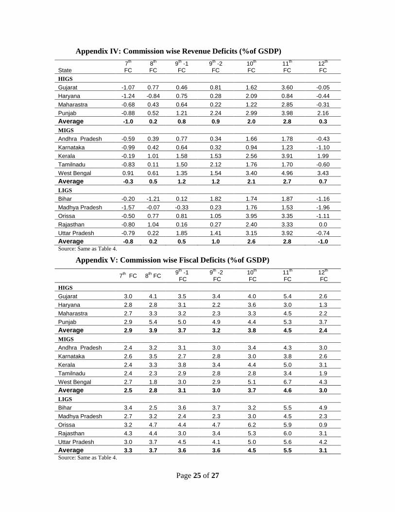
Thus depending on the relative benefits of the traditional methods and the new
programmes, states started increasing or decreasing deficits (see appendix IV & V).
However, the better off states could play the game more tactfully than the poorer states
due to their large budget size. They are Gujarat, Maharastra and Punjab among the HIGS
and Kerala and West Bengal among the MIGS. Elsewhere it has been stated that
Maharastra, Punjab, Kerala and West Bengal have been failed to achieve the targets of
FRBMA (Ravishankar, Zahir and Kaul 2008, p 60). While Gujarat and West Bengal have
declined their own revenue effort and thereby reducing the amount of own revenue the
other three have increased the revenue expenditures.
Part V
5. Conclusion
With diverse socio-economic characteristics of the country, federal structure of
government has been adopted to provide all nationals common minimum level of basic
public goods per unit of tax price. Even if the design of the structure is in line with the
economic principle of fiscal federalism, fiscal imbalances are found to be increasing
overtime. The complementarities of methods having same objectives and contradicting
methods with different objectives of UFC and PC create a paradox in the process of
central devolution which accentuated fiscal imbalances. Rich states have been
discouraged to improve their revenue capacity imposing revenue burden on people when
equity objective is given more emphasis. In the same line poor states suffer when higher
weightage is assigned to efficiency criterion. With this conflicting situation reforms in the
transfer system are of crucial importance which should be considered by the 14th
FC.

Page 23 of 27
Appendices
Appendix I: Deficits of Centre, States
Deficits of Centre Deficits of State
RD%GDP RD%FD FD%GDP PD%GDP RD%GDP RD%FD FD%GDP
PD% GDP
1980-81 1.5 24.5 6.1 4.2 -1.1 -40.0 2.7 1.8
1981-82 0.2 4.5 5.4 3.4 -0.9 -33.9 2.5 1.6
1982-83 0.7 12.3 5.9 4.9 -0.5 -17.8 2.8 1.8
1983-84 1.2 19.5 6.2 3.9 -0.1 -3.3 3.0 2.1
1984-85 1.8 24.3 7.4 4.9 0.4 11.3 3.5 2.4
1985-86 2.2 26.9 8.3 5.5 -0.2 -8.7 2.9 1.7
1986-87 2.7 29.5 9.0 5.8 -0.1 -1.8 3.2 1.8
1987-88 2.8 33.8 8.1 4.8 0.3 9.7 3.4 1.9
1988-89 2.7 34.0 7.8 4.2 0.5 15.5 2.9 1.4
1989-90 2.6 33.4 7.8 3.9 0.8 23.9 3.4 1.8
1990-91 3.5 41.6 8.4 4.4 1.0 28.3 3.5 1.9
1991-92 2.7 44.8 5.9 1.6 0.9 29.9 3.1 1.3
1992-93 2.6 46.3 5.7 1.3 0.7 24.5 3.0 1.1
1993-94 4.0 54.3 7.4 2.9 0.5 19.0 2.5 0.6
1994-95 3.2 53.8 6.0 1.4 0.7 24.6 2.9 0.8
1995-96 2.7 49.4 5.4 0.9 0.8 27.9 2.8 0.8
1996-97 2.5 48.9 5.1 0.6 1.3 46.2 2.8 0.9
1997-98 3.2 52.2 6.1 1.6 1.2 40.2 3.0 0.9
1998-99 4.0 59.1 6.8 2.1 2.7 60.7 4.4 2.3
1999-2000 3.6 64.6 5.6 0.8 2.9 60.5 4.8 2.4
2000-01 4.3 71.7 5.9 1.0 2.8 62.9 4.4 1.8
2001-02 4.6 71.1 6.5 1.5 2.8 64.1 4.3 1.5
2002-03 4.6 74.4 6.2 1.2 2.4 57.3 4.3 1.3
2003-04 3.7 79.7 4.7 0.0 2.4 52.6 4.6 1.5
2004-05 2.6 62.3 4.2 0.0 1.3 36.3 3.6 0.7
2005-06 2.7 63.0 4.3 0.4 0.2 7.8 2.7 0.2
2006-07 2.0 56.3 3.6 -0.2 -0.6 -32.1 2.0 -0.4
2007-08 1.1 41.4 2.8 -1.0 -0.9 -56.9 1.6 -0.5
2008-09 4.8 75.2 6.4 2.7 -0.2 -9.4 2.5 0.6
2009-10 5.5 81.0 6.8 3.3 0.5 16.4 3.1 1.2 Sources: For GDP at Current Prices, CSO website, http://mospi.nic.in/Mospi_New/site/home.aspx and for
Deficits the same source as Table 1.

Page 24 of 27
Appendix II: Change of indicators of State Finances from 10th
to 11th
FC (% of
GSDP)
States OR CST GR RR RE RD
HIG
Gujarat 0.10 -0.35 0.58 0.32 2.30 1.98
Haryana -1.70 -0.40 -0.14 -2.24 -3.50 -1.25
Maharastra 0.70 -0.18 -0.04 0.49 2.10 1.63
Punjab 1.90 -0.19 0.08 1.79 3.00 0.99
MIG
Andhra Pradesh 1.50 -0.63 0.12 0.99 1.30 0.12
Karnataka 2.10 0.02 0.36 2.48 1.70 0.30
Kerala 0.10 -0.24 -0.04 -0.18 1.20 1.35
Tamilnadu 1.00 -0.20 0.15 0.95 0.90 -0.06
West Bengal 0.10 0.33 0.34 0.77 2.30 1.56
LIG
Bihar 0.60 2.93 0.93 4.47 4.30 0.13
Madhya Pradesh 1.30 1.07 0.30 2.67 2.40 -0.24
Orissa 1.50 1.20 0.13 2.83 0.40 -0.61
Rajasthan 0.70 0.64 0.44 1.77 2.70 0.94
Uttar Pradesh 1.40 1.25 0.38 3.03 3.80 0.77
Note: Same as Table 5.
Source: Same as Table 1.
Appendix III: Change of indicators of State Finances from 11th
to 12th
FC (%of
GSDP)
States OR ST GR RR RE RD
HIG
Gujarat -1.17 0.51 -0.13 -0.79 -4.43 -3.65
Haryana 0.21 0.29 0.22 0.72 -0.56 -1.29
Maharastra -0.32 0.19 0.89 0.76 -2.41 -3.17
Punjab -0.40 0.45 0.78 0.83 -1.00 -1.83
MIG
Andhra Pradesh 1.86 0.84 0.68 3.39 0.96 -2.22
Karnataka 1.30 0.19 0.60 2.09 -0.24 -2.34
Kerala 0.04 0.24 0.43 0.71 -1.20 -1.92
Tamilnadu 1.10 0.43 0.60 2.13 -0.17 -2.30
West Bengal 0.37 0.48 0.33 1.18 -0.35 -1.53
LIG
Bihar 0.41 2.83 1.91 5.15 1.79 -3.03
Madhya Pradesh 0.87 1.30 1.50 3.67 0.18 -3.49
Orissa 0.81 0.76 1.04 2.61 -1.85 -4.46
Rajasthan 1.28 1.05 0.23 2.55 -0.79 -3.33
Uttar Pradesh 1.94 2.36 1.44 5.74 1.07 -4.66
Note: Same as Table 5.
Source: Same as Table 1.
Page 25 of 27
Appendix IV: Commission wise Revenue Deficits (%of GSDP)
State 7
th
FC 8
th
FC 9
th -1
FC 9
th -2
FC 10
th
FC 11
th
FC 12
th
FC
HIGS
Gujarat -1.07 0.77 0.46 0.81 1.62 3.60 -0.05
Haryana -1.24 -0.84 0.75 0.28 2.09 0.84 -0.44
Maharastra -0.68 0.43 0.64 0.22 1.22 2.85 -0.31
Punjab -0.88 0.52 1.21 2.24 2.99 3.98 2.16
Average -1.0 0.2 0.8 0.9 2.0 2.8 0.3
MIGS
Andhra Pradesh -0.59 0.39 0.77 0.34 1.66 1.78 -0.43
Karnataka -0.99 0.42 0.64 0.32 0.94 1.23 -1.10
Kerala -0.19 1.01 1.58 1.53 2.56 3.91 1.99
Tamilnadu -0.83 0.11 1.50 2.12 1.76 1.70 -0.60
West Bengal 0.91 0.61 1.35 1.54 3.40 4.96 3.43
Average -0.3 0.5 1.2 1.2 2.1 2.7 0.7
LIGS
Bihar -0.20 -1.21 0.12 1.82 1.74 1.87 -1.16
Madhya Pradesh -1.57 -0.07 -0.33 0.23 1.76 1.53 -1.96
Orissa -0.50 0.77 0.81 1.05 3.95 3.35 -1.11
Rajasthan -0.80 1.04 0.16 0.27 2.40 3.33 0.0
Uttar Pradesh -0.79 0.22 1.85 1.41 3.15 3.92 -0.74
Average -0.8 0.2 0.5 1.0 2.6 2.8 -1.0
Source: Same as Table 4.
Appendix V: Commission wise Fiscal Deficits (%of GSDP)
7
th FC 8
th FC
9th
-1 FC
9th
-2 FC
10th
FC
11th
FC
12th
FC
HIGS
Gujarat 3.0 4.1 3.5 3.4 4.0 5.4 2.6
Haryana 2.8 2.8 3.1 2.2 3.6 3.0 1.3
Maharastra 2.7 3.3 3.2 2.3 3.3 4.5 2.2
Punjab 2.9 5.4 5.0 4.9 4.4 5.3 3.7
Average 2.9 3.9 3.7 3.2 3.8 4.5 2.4
MIGS
Andhra Pradesh 2.4 3.2 3.1 3.0 3.4 4.3 3.0
Karnataka 2.6 3.5 2.7 2.8 3.0 3.8 2.6
Kerala 2.4 3.3 3.8 3.4 4.4 5.0 3.1
Tamilnadu 2.4 2.3 2.9 2.8 2.8 3.4 1.9
West Bengal 2.7 1.8 3.0 2.9 5.1 6.7 4.3
Average 2.5 2.8 3.1 3.0 3.7 4.6 3.0
LIGS
Bihar 3.4 2.5 3.6 3.7 3.2 5.5 4.9
Madhya Pradesh 2.7 3.2 2.4 2.3 3.0 4.5 2.3
Orissa 3.2 4.7 4.4 4.7 6.2 5.9 0.9
Rajasthan 4.3 4.4 3.0 3.4 5.3 6.0 3.1
Uttar Pradesh 3.0 3.7 4.5 4.1 5.0 5.6 4.2
Average 3.3 3.7 3.6 3.6 4.5 5.5 3.1
Source: Same as Table 4.

Page 26 of 27
References
Ahluwalia, Montek (2000): “Economic Performance of States in Post Reform Period”, Economic
and Political Weekly, Vol. XXXV, No. 19, May 6, pp 1637-48.
Bagchi, Amaresh and Pinaki Chakraborty (2004): “Towards a Rational System of Centre- State
Revenue Transfers”, Economic and Political Weekly, Vol. XXXIX, No.26, June 26-July
2, pp 2737-2747.
Chakraborty, P (1998): “Growing Imbalances in Federal Fiscal Relationship”, Economic and
Political Weekly, Vol. XXXIII, No.7, February 14-20, pp 350-354.
Chakraborty, P (2010): “Deficit Fundamentalism vs Fiscal Federalism: Implications of 13th
Finance Commission‟s Recommendations”, Economic and Political Weekly, Vol. XLV,
No.48, November 27-Decembe 3, pp 65-63.
Chelliah, R J (2005): “Malady of Continuing Fiscal Imbalance”, Economic and Political Weekly,
Vol. XL, No.31, July 30-August 5, pp 3399-3404.
Chelliah, Raja J, M G Rao and T K Sen (1992): “Issues before Tenth Finance Commission”,
Economic and Political Weekly, Vol. XXVII, No.47. , November 21-27, pp 2539-2550.
Ghosh, Jayati (2005): “Twelfth Finance Commission and Restructuring of State Government
Debt: A Note.” Economic and Political Weekly, Vol. XL, No.31 July 30 – August 5, pp
3435-3439.
Kannan, R; S N Pillai; R Kausaliya and Jai Chander (2004): “Finance Commission Awards and
Fiscal Stability in States”, Economic and Political Weekly, Vol. XXXIX. No.5, January
31- August 5, pp 3399-3404.
Kurian, N J (2005): “Debt Relief for States” Economic and Political Weekly, Vol. XL, No.31,
July 30 - August 5, pp 3429-34, .
Lalvani, Mala (2009): “Persistence of Fiscal Irresponsibility: Looking Deeper into Provisions of
FRBM Act”, Economic and Political Weekly, Vol. XLIV, No. 37, September 12, pp 57-
63.
Mukhopadhyay, Hiranya and Kuntal Kumar Das (2003): “Horizontal Imbalances in India: Issues
and Determinants”, Economic and Political Weekly, Vol. XXXVIII. , No.14, April 5-11,
pp 1416-1420
Mukhopadyay, Debes (2003): “Centre State Financial Relations in India”, in P K Chaubey, (eds.),
Fiscal Federalism in India, Deep and Deep Publications PVT. LTD., New Delhi.
Raju, Swati (2012): “Growth across States in 2000: Evidence of Convergence”, Economic and
Political Weekly, Vol. XLVII, No 23, June 9, pp 76-79.

Page 27 of 27
Rakshit, M (2005): “Some Analytics and Empirics of Fiscal Restructuring in India”, Economic
and Political Weekly, Vol. XL, No 31, July 30 - Aug 5, pp 3440-3449.
Rangarajan, C (2005): “Approach and Recommendations”, Economic and Political Weekly, Vol.
XL, No 31, July 30 to August 5, pp 3396-3398.
Rangarajan, C and D K Srivastava, (2005): “Fiscal Deficit and Government Debt: Implications
for Growth and Stabilization”, Economic and Political Weekly, Vol. XL, No. 27 July 2,
pp .2919-2934.
Rao, M G and P R Jena (2005): “Balancing Stability, Equity and Efficiency”, Economic and
Political Weekly, Vol. XL, No.31, July 30-August 5, pp 3405 -12.
Rao, M G (2000): “Linking Central Grants to Revenue Deficit Reduction by States”, Economic
and Political Weekly, Vol. XXXV, No 23, June 3-9, pp 1883-84.
Rao, M G (2002): “State Finances in India: Issues and Challenges”, Economic and Political
Weekly, Vol. XXXVII, No 31, August 3-9, pp 3261-3271.
Rao, M G (2003): “Incentivizing Fiscal Transfers in the Indian Federation”, The Journal of
Federalism, Vol. XXXIII, No .4.
Rao, M G (2004): “Linking Central Transfers to Fiscal Performance of States”, Economic and
Political Weekly, Vol. XXXIX, No.18, May 1-6, pp 1820-1825.
Rao, M G & Nirvikar Singh (2005): “Asymmetric Federalism in India.” in Richard Bird and
Robert Ebel, Fiscal Fragmentation in Decentralized Countries: Subsidiary, Solidarity
and Asymmetry.
Rao, M G and T K Sen (1996): Fiscal Federalism in Theory and Practice, New Delhi, Indian
Council of Social Science Research.
Spant, Ronald (2003): “Why Net Domestic Product Should Replace Gross Domestic Product as a
Measure of Economic Growth” International Productivity Monitor, No.7, pp 39-43
Varghese, Santhosh (2006): “Fiscal Responsibility or Fisc‟s Liability? Some Quick Comments on
the Impact of Fiscal Targets in FRBM Acts of Sub-national States”, Paper Submitted as
Part of Refresher Course in Public Economics, 28 May-22 June, 2006.