The Paradox of Civilization

Pre-Institutional Sources of Security and Prosperity

Ernesto Dal Bo Pablo Hernandez Sebastian Mazzuca∗

July 2016

Abstract

The rise of civilizations involved the dual emergence of economies that could pro-

duce surplus (“prosperity”) and states that could protect surplus (“security”). But

the joint achievement of security and prosperity had to escape a paradox: prosperity

attracts predation, and higher insecurity discourages the investments that create pros-

perity. We study the trade-offs facing a proto-state on its path to civilization through

a formal model informed by the anthropological and historical literatures on the ori-

gin of civilizations. We emphasize pre-institutional forces, such as physical aspects

of the geographical environment, that shape productive and defense capabilities. The

solution of the civilizational paradox relies on high defense capabilities, natural or man-

made. We show that higher initial productivity and investments that yield prosperity

exacerbate conflict when defense capability is fixed, but may allow for security and

prosperity when defense capability is endogenous. Some economic shocks and military

innovations deliver security and prosperity while others force societies back into a trap

of conflict and stagnation. We illustrate the model by analyzing the rise of civilization

in Sumeria and Egypt, the first two historical cases, and the civilizational collapse at

the end of the Bronze Age.

∗Dal Bo: UC Berkeley and NBER. Hernandez: NYU AD. Mazzuca: Johns Hopkins. We thank RobertAllen, Pedro Dal Bo, Santiago Oliveros, Ben Olken, Demian Pouzo, Robert Powell, Alvaro Sandroni, DavidSchonholzer and Enrico Spolaore for valuable discussion, as well as seminar and conference participants forhelpful comments.

1 Introduction

Anatomically modern humans have lived in subsistence and stateless societies for roughly

97% of their 200,000-year-long history. If there is a Big Bang in human history, it occurred

as recently as 5,000 years ago, when the first civilizations emerged. Civilization meant fun-

damental transformations: systematic surplus production, urbanization, public architecture,

writing, and states. Although the rise of civilization is arguably more of a qualitative change

than the Industrial Revolution, modern political economy has paid much less attention to

it.

According to an influential view in archaeology, the rise of civilizations is primarily driven

by an exceptional potential for food production, both in terms of endowments and technology.

For V. Gordon Childe, the key features of Lower Mesopotamia, the “cradle of civilization,”

were an extremely fertile alluvial soil, an abundance of edible animals, and irrigation tech-

nology. Identical factors were emphasized for the rise of Egypt, the first pristine civilization

after Sumer. Both in Lower Mesopotamia and Egypt “irrigation agriculture could generate a

surplus far greater than that known to populations on rain-watered soil” and “as productivity

grew, so too did civilization” (Mann 1986: 80, 108).

Without a substantial surplus, it was not possible to fund the tangible components of

civilizations. However, surplus production was only a necessary condition for civilization, not

a sufficient one. In fact, prosperity could be self-defeating. Primitive food producers were

surrounded by nomadic tribes for whom agricultural surpluses were a most tempting target

for looting. The resulting clash is a primordial conflict shaping the civilizational process.

According to McNeill (1979, p. 71), “Soon after cities first arose ... the relatively enormous

wealth that resulted from [their economic activity] made such cities worthwhile objects of

attack by armed outsiders.” For anthropologists, intergroup violence had been prevalent

since before civilization (Keeley 1996), but the emergence of large surpluses intensified the

potential for conflict. According to Michael Mann, “the greater the surplus generated, the

more desirable it was to preying outsiders” (1986: 48).

Since civilization entailed the joint achievement of prosperity and security, its emergence

is a fundamental paradox. Primitive societies that held production close to subsistence levels

could hope to mitigate predation, but stagnation would foreclose the civilization process.

To reach civilization, primitive societies with the capacity for surplus production had to

1

overcome the dangers of self-defeating prosperity without relying on the relative safety of

stagnation. A proper balance was needed between surplus production and surplus protection.

The contextual conditions allowing for such a balance are rare, as evidenced by the fact

that, out of thousands of primitive societies, only a handful could develop independent civ-

ilizations, starting with Sumer and Egypt. In this paper we develop a model to identify

the logical conditions for successful civilization, and examine for the first time the historical

record for the rise of Sumer and Egypt under the perspective of the civilizational paradox.

The historical cases illustrate the logic of the model, and the model allows for a richer in-

terpretation of the cases. Sumer and Egypt provide evidence that the potential for surplus

emphasized by archaeologists and geographers was only half of the story of successful civi-

lization. The other half was surplus protection. In addition to their historical preeminence

as cases achieving the right balance between prosperity and security, Sumer and Egypt illus-

trate that protection occurs in two contrasting ways—defense can be natural as in Egypt,

or man-made as in Sumer.

The rise of civilization, and its intrinsic paradox, can be usefully compared to the rise of

the modern state in the post-Westphalia context, another major turning point in history. The

rise of the modern state also involves a paradox. European rulers striving for a monopoly of

violence were able to reach unprecedented levels of power but in the process they undermined

their own ability to credibly commit to respecting private rights. Unstable property rights

in turn diminished the capacity of the underlying society to grow, and ultimately damaged

the ruler’s own power. The standard insight is that the solution for the modern state was

“institutions” understood as rules of the political game: checks and balances, as well as the

expansion of political rights, helped the ruler to solve its credibility problem either vis-a-vis

society at large or vis-a-vis competing factions within the elite (North and Weingast 1989,

Acemoglu and Robinson 2005, Lizzeri and Persico 2004).

In contrast to the solution to the paradox of the modern state, the solution to the

paradox of civilization in our approach does not involve institutions. The joint achievement

of order and prosperity in the context of pristine civilizations is a pre-institutional process,

involving tangible assets and technologies, of either economic or military nature. Pristine

civilizations emerged in areas with exceptional natural endowments for food production, and

the man-made contributions to the civilizational breakthrough were not political rules, as

institutional theories would emphasize, but productive and defense equipment. Two massive

2

engineering accomplishments are the mark of the Ancient Near East: irrigation infrastructure

in both Egypt and Sumer, and perimetral walls in cities throughout Mesopotamia and the

Levant. Each public good had a single, well-defined mission: surplus production and surplus

protection. The prominence of the two types of public works reflects the centrality of the

production-protection tension in the process of civilization building.

Our pre-institutional theory on the joint achievement of security and prosperity can help

improve our understanding of the rise of the first civilizations, and shed light on the problem

of state formation more generally. A broader goal is to generate insights for a wide class

of development trajectories in which a potentially prosperous region, being surrounded by

predatory threats, may fall in the traps of security-enhancing stagnation or self-defeating

prosperity. This class includes the interaction between a large number of proto-cities and

barbarian invaders from the steppes across the Eurasian continent throughout the Middle

Ages; the long struggle in 19th century Latin America between elites from port-cities en-

gaged in nation-building and rural warlords, “caudillos,” dominating the periphery; as well

as contemporary state-building efforts in failed states of Sub-Saharan Africa and the Mid-

dle East, in which international economic aid, if not coupled with military buildup, may

have counter-productive effects by inducing voracity among neighbors. Echoing concerns

in history and anthropology about the reversibility of gains in social complexity that lead

to statehood, our theory provides an account for civilization collapse, and more generally

for economic or military reversals in societies that had achieved prosperity and security.

For illustration, we will use the model to account for the End of the Bronze Age, a much-

debated process in which dozens of civilization centers collapsed rather quickly throughout

the Eastern Mediterranean, ushering in the first “dark ages” in the historical record.

1.1 Overview of the model

In our model, a population in control of an economy with the potential to create surplus (the

“incumbent”) faces potential attacks by a predatory group (the “challenger”). The incum-

bent has the opportunity to invest and grow future income, which would lead to “prosperity;”

however, the possibility of attacks may recommend spending resources in consumption and

defense instead. Three key parameters are the initial productivity (or income), and the rates

at which consumption can be turned into defense (defense capability) and future income

3

(growth capability). Higher initial productivity helps finance more defense, but it also at-

tracts stronger predation. If sufficient defense can be financed, the challenger is deterred

(“security” is attained). Productive investment may also intensify predatory challenges by

raising future income. The result is a tradeoff between investment-led growth and secu-

rity. The key formal question is whether some combination of parameter values allows for

productive investment and deterrence to yield a civilizational breakthrough.

In the first part of our analysis the incumbent’s defense capability is exogenous, and in the

second part defense capability can be improved. Both parts help rationalize different modal-

ities in the rise of ancient civilizational states. The analysis in the first part characterizes the

unique equilibrium of the game. The key result is that the parameter space is partitioned

into four regions corresponding to the four possible “prosperity/security” combinations.

When both defense and growth capabilities are low, neither prosperity nor security are

possible, and societies remain locked in the situation of economic stagnation and conflict

characterized by Keeley (1996), which corresponds to the Hobbesian “state of nature.”1 If

growth capability is high relative to defense capability, prosperity becomes possible even in

the face of attacks. Although anti-Hobbesian, the possibility of growth despite predation is

consistent with a widespread occurrence in the history of humanity, like the Chinese with

the Mongolians and the Saxons with the Vikings in the 10th century. Lastly, when both

defense and growth capabilities are high and “balanced,” the incumbent can grow and also

deter predators. The latter two cases are the key to our explanation for the emergence of

civilizations. Civilizations occur in cases where high enough returns to productive investment

allow the economy to grow, and where the incumbent manages to deter attacks by the

challenger, or, if attacks occur, to repel them with reasonably high probability.

The case of Egypt can be explained in terms of natural endowments for both growth

and (exogenous) defense. Growth capabilities were given by rich alluvial soils that could

be quickly improved through productive investments, and defense was provided by the sur-

rounding deserts, which protected dwellers along the Nile from most types of attack (Bradford

2001).

1The relationship between security and prosperity has been a perennial concern in the social sciences.A dominant view, inspired by Hobbesian philosophy, is that state-provided security is a precondition forprosperity (Lane 1958; Olson 2000; Bates 2001; see Boix 2015 for a contrasting approach). But the stateitself has to be explained and the Hobbesian view provides no clear message on whether state formationrequires a modicum of prosperity in the first place.

4

The model allows us to study how shocks (natural, or policy-originated) to defense

and growth capabilities can generate transitions from one area to another in the security-

prosperity outcome space. Such shocks can account not only for the rise of civilizations,

but also for their fall and the loss of security and prosperity, ushering in “dark ages.” We

illustrate this case with a study of the end of the Bronze Age around 1200BC. Our model

also shows that enhanced defense capabilities are a necessary condition for achieving security

and prosperity, but expanding growth capability, while valuable, is not strictly necessary.

Moreover, under certain conditions, improved growth capabilities may worsen outcomes.

The rise of civilization in Southern Mesopotamia poses a challenge to our model with

exogenous defense capability, because the Sumerian settlements, in contrast with Egypt, did

not have natural protection. Rather, as widely attested in the archaeological record, they

faced challenges from various pastoralist groups. Then, how could the Sumerian city-states

ever emerge? According to the anthropological literature, the settled groups that formed

pristine states exploited an agrarian “staple finance”, which, being highly rewarding, would

fund their defense (Johnson and Earle 2000, p. 305-306). These groups had a material

advantage that could be turned into a military one, by relying on walls, weaponry, and num-

bers, all of which could be used to deter or defeat their enemies. This process of endogenous

improvement of defense capabilities can be accounted for in our extended model, where the

incumbent can make investments to upgrade defense. We show that when initial produc-

tivity is high enough the incumbent can fund its way out of the parametric region without

security or prosperity into a region with high levels of both.

While higher initial productivity always exacerbates conflict in the model with exogenous

defense capability, in the model with endogenous defense it may pave the way to security and

prosperity. That this should happen is not obvious, since improvements in defense capability

are an investment, and as such they are discouraged by the insecurity associated with higher

initial productivity. When stronger defense capability is put in place, a Hobbesian effect

is observed: the enhanced security yields a higher effective return to productive investment

and it fosters prosperity.

5

1.2 Plan for the paper

In the next section we relate our contribution to existing literature. In section 3 we present

the model with exogenous defense capability, and use it in section 4 to analyze the rise

of Egypt and the end of the Bronze Age. In section 5 we extend the model to allow for

endogenous defense capability, and in section 6 we use the extended model to account for

the rise of Sumeria. We conclude in section 7.

2 Related Literature

Archaeologists like V. Gordon Childe (1936), who first conceptualized the advent of the

Neolithic era as an “agricultural revolution,” focused on the innovations in the means and

relations of production while abstracting from the necessary accompanying innovations in

military protection. On the other hand, several archaeologists have noted the paramount role

of investments in protection, such as fortifications, walls, and moats, in the erection of the

first cities (Service 1975, 299). According to Near Eastern archaeologist Volkmar Fritz, “in

the Jordan Valley, settlements were surrounded by a wall even before it is possible to speak of

the city proper” (1997 II: 19). Other authors, like Mann (1986) and McNeill (1979), explicitly

connected food production with protection needs, as mentioned earlier. However, we are not

aware of any account that has explicitly focused on the interplay of surplus production and

surplus protection to point out a solution to the civilizational paradox. As we will show, the

interplay is subtle and perhaps profitably analyzed through a formal model.

Our approach builds on, but departs from, historical accounts that emphasize the ge-

ographic sources of economic prosperity. The approaches emphasizing the availability of

domesticable plants and animals to explain why some regions generated surpluses while oth-

ers did not (e.g., Diamond 1999) contribute a necessary building block for understanding the

prosperity of the first settled societies. However, a purely geographic approach is incomplete,

for it misses the role of incentives and strategic action that is at the core of any viable socio-

political account of the origin of civilizations. Our approach incorporates both strategic

actors and geographic factors such as food production potential or protective terrain.

Our investigation comes at the cost of abstracting from some aspects that have been

6

considered in anthropological theories of the state.2 For example, an influential view in

anthropology is that the state emerged to sustain and expand economic inequality (Fried

1960, 728). We abstract from social hierarchy not because we think political stratification is

unimportant, but because it helps to focus attention on the incumbent-challenger interaction.

For Carneiro (1970), states originated in fertile areas surrounded by less productive land.

Growing populations would contest fertile land and losers, unable to flee, would accept

domination. The ensuing political stratification is the basis of the state. The Nile valley,

surrounded by deserts, is a good example of circumscribed productive land. Our model

generates a similar empirical implication; however, it is not driven by exploitation but by

the fact that low quality surrounding land can protect against challengers. Unlike Carneiro’s

theory, our model does not appeal to population pressure, an assumption that has been

challenged by some writers (see Allen 1997).

It is customary in the social sciences to view the state as the monopoly on violence.

Adapting from Weber, we define the state not in binary terms but as a matter of degrees

(Weber 1978: ch. I, s. 16), so that state formation involves higher degrees of protection

from attacks. We focus on the state as “sovereignty,” defense from threats, and abstract

from “rulership,” the creation of a political hierarchy and institutions within a society, which

even critics of the institutional approach include in their definition (see Boix 2015: 66-77).

The exclusion of both rulership and political institutions from our model helps identify a

minimalist view of early civilizations as the intersection of surplus production and statehood

seen as sufficient surplus protection.

Our work is related to both theories of state formation (Tilly 1975, 1992, Spruyt 1996)

and theories of the political sources of prosperity (North and Weingast 1989; Olson 2000,

Bates 2001; Boix 2015). In contrast to our model, theories of state formation do not place

the state in the context of the “security-prosperity” tradeoff, and theories of the political

sources of prosperity focus on rules of the political game once the state is already in place

rather than on pre-state forces.3

Our work has important complementarities with that by Mayshar, Moav and Neeman

2For a review of anthropological theories of early states see for example Claessen and Skalnik (1978).3We share with Boix (2015) an interest in mechanisms of state formation extending back into prehistoric

times, as well as in “hard” causes related to the physical environment. Although Boix finds sources of pre-institutional cooperation under conditions of anarchy (absence of state), he conceives of state formation asthe selection of either republican or monarchic institutional settings. By contrast, we focus on the conditionsfor state formation that allow for investment and security before political institutions become central.

7

(2013), and Mayshar, Moav, Neeman and Pascali (2015). They also combine a focus on

early states, an emphasis on geographic drivers, and the use of formal theory. For us, ge-

ography matters because it defines both productive and defense capabilities, while for them

it determines the observability of production (the former paper) or its appropriability (the

latter). Mayshar, Moav and Neeman (2013) use a principal-agent model to show how mon-

itoring capabilities shape the extent of political centralization, and account for contrasting

trajectories in Sumeria and Egypt, where observability of the Nile allowed for a more unified

and lasting state. Our focus is not on the form of states, but on the conditions for their

emergence. This is also the focus of Mayshar, Moav, Neeman and Pascali (2015), who focus

on crop appropriability. They equate the state with the political hierarchy that results from

appropriability and assume it results in the full prevention of conflict. We abstract from

appropriability and internal hierarchy, and investigate whether it is true that conflict can be

reduced or eliminated.

A recent literature studies the incentives to make investments in state capacity in sit-

uations where the ruler may lose control of the polity to a competing faction (Besley and

Persson 2011), or to a foreign power (Gennaioli and Voth 2015). Gennaioli and Voth (2015)

formalize and investigate empirically Tilly’s (1990) argument that modern European states

formed as a result of the competitive pressures of military conflict, which created a need to

centralize fiscal control. There are some differences in terms of modeling: unlike in Besley

and Persson’s model, investments in our model can augment the virulence of challenges, and

we abstract from the competitive dynamics between states that anchor Gennaioli and Voth’s

analysis. There are differences in substantive focus as well. In the state capacity literature

there is a pre-existing state, while we focus in pre-state societies that move towards state-

hood by attaining some degree of deterrence. Our paper is also related to models of state

consolidation (Powell 2012, 2013); the key difference is that in our model consolidation is

studied in relation to investment and growth.

Our work is obviously related to the literature on conflict, which is too extensive to re-

view here, in particular the family of papers investigating the tradeoff between “guns” and

“butter” (see Garfinkel and Skaperdas 2007 for a review), the closest of which is perhaps the

paper by Grossman and Kim (1995), where agents choose between production and contesta-

tion. Our model differs at least in two respects: we consider a dynamic environment where

investments and growth affect future consumption and means for defense, and we endogenize

8

the productivity of war efforts.

3 The Basic Model

3.1 Setup

Our baseline model features the incentives to raise an army to protect wealth from usurpers

at the cost of resources for consumption or productive investment. Later on we introduce

the decision to invest in defense capability.

Players An “incumbent” lives for two periods t = 1, 2, and controls a productive asset

that yields a nonstorable flow vt > 0, in each period. The asset can be a piece of land, a port,

or any bundle of productive resources including people. The initial level v1 tracks properties

of the environment (e.g., weather, quality of the soil, topography) that affect the quantity

and value of goods that the economy can produce, i.e., productivity. The incumbent faces

a “challenger” in each period, who is interested in wresting control of the productive asset

away from the incumbent.4 This interaction captures the large class of cases of inchoate

urban centers (agricultural settlements, city-ports, markets at the crossing of interior roads)

where food-producing populations or trading elites face the threat of predatory attacks by

nomadic tribes or plundering warlords.

Actions, resources and technology In each period t the incumbent can spend its flow

vt on consumption, productive investment it or mobilizing resources to defend its asset. One

dollar of productive investment it costs one dollar of consumption and it adds ρ > 1 dollars

to the yield of the productive asset in the future.5 That is, productivity evolves according to

the relation vt+1 = vt + ρit; we abstract from depreciation and discounting for simplicity. ρ

captures anything that affects the returns to productive investments in the asset controlled

by the incumbent. For example, ρ could, like v1, reflect various conditions of the physical

environment such as climatic conditions and soil fertility, or economic factors such as the

price of goods sold.6

4In the basic model it does not matter whether the challenger is different across periods or not. In themodel with endogenous defense capability we assume the challenger is different each period.

5Given that for ρ < 1 investment is never worthwhile, failure to obtain it in equilibrium is obvious anduninteresting. Hence our assumption ρ > 1 which makes investment at least a possibility.

6If the value of what the incumbent produces follows a standard price × quantity formulation we canwrite v1 = pq, and v2 = v1 + ρpi = pq + ρpi, where q and i are physical units. Then, changes in p will

9

The effectiveness of the incumbent’s defense (or “army”) is denoted at and such an army

costs the challenger an amount atκt

where κt ≥ 0 is the value of the incumbent’s defense

capability. The higher the defense capability of the incumbent, the higher the “firepower”

at attained by a given conflict effort atκt

. κt captures anything that affects the costs for the

incumbent of producing defense or military firepower, such as a rugged terrain or better

military technology or expertise.7 In this section κt is fixed at an initial level κ1 and we will

derive implications for conflict and prosperity stemming from different values of κ1. The

extended version of the model in section 5 will be devoted to endogenizing κt.

In period t the incumbent faces a budget constraint,

vt − it −atκt≥ 0. (1)

The challenger observes the choices of at and it by the incumbent and chooses its own

conflict effort bt.8 If victorious in the first period the challenger captures the incumbent’s

income in the second period; in a two period model it is immaterial whether expropriation

involves the income flow or the asset itself. Whenever the challenger attacks (bt > 0), it

prevails with probability btat+bt

and it gains nothing with the complementary probability

(i.e., we adopt the typical Tullock contest success function).9 If the incumbent is defeated

it obtains an outside payoff normalized to zero. If the challenger selects bt = 0 we say

the incumbent has successfully deterred the challenger, and this lack of challenge to the

authority of the incumbent results in full security. As we explain later, we associate the

degree of security–be it in terms of internal order or external sovereignty–with the degree of

statehood, so full security corresponds to full statehood.

cause changes in both v1 and ρ. Changes in the baseline physical capacity of production q will be capturedthrough changes in v1 exclusively, and changes in the physical returns to investment as changes in ρ only.

7One interpretation is that the incumbent has a stock κt (e.g., a wall or a catapult) that is complementaryto current army effort et. They jointly produce an army power at = κtet and so given κt, the cost of theeffort expense e is at

κt. To save on notation we obviate the term et.

8Assuming that the challenger’s war expense is basically effort is equivalent to assuming that the chal-lenger’s income is sufficient to finance the optimal war effort b∗t . Because the effects of interest are not drivenby a budget constraint on the challenger being binding, we follow the most parsimonious approach of notintroducing a positive income nor a resource constraint for the challenger.

9Generalized versions of the ratio-based contest success function exist but are less tractable. Hirshleifer(2001) explores some of the difficulties. The typical generalization is to consider functions of the type aα

aα+bα .The most important feature of our model, which is the possibility of generating deterrence, will obtain forany function satisfying α ∈ [0, n/(n− 1)] in a symmetric contest with n players. For α > n/(n − 1) purestrategy equilibria cease to exist.

10

Timing In each period the incumbent selects at and it. After observing (at, it) the

challenger selects bt. If b1 = 0, the incumbent remains in place in period 2. If b1 > 0, then

there is conflict at the end of period 1. The winner obtains the incumbent’s income in period

2.10 The challenger obtains zero in the event of no attack.

Payoffs Both challenger and incumbent are risk neutral and care linearly about con-

sumption, which equals income net of costs of investment and defense. The incumbent acts

as a Stackelberg leader, choosing a1 and i1 to maximize the value Vt:

Vt = vt −atκt− it +

atat + bt

Vt+1. (2)

The challenger chooses bt to maximize the expression

Wt =bt

at + btVt+1 −

btκc, (3)

where Vt+1 = vt + ρit, and where κc is the military capability of the challenger. We could

also parametrize the challenger’s objective with a factor h and write the expected benefit as

btat+bt

hVt+1, so as to capture different levels of “hunger” by the challenger.11 The parameter

h would capture a different substantive aspect than κc, but it would be mathematically

redundant since the challenger’s problem could be rewritten as involving a military capability

of hκc instead. Therefore we will abstract from the parameter h. To simplify notation, we will

develop the model normalizing κc = 1, and will comment later on how the solution changes

with variations in κc. An additional simplification is we do not consider here the realistic

possibility that conflict destroys part of the asset. Our results do not change qualitatively if

conflict generates some destruction.12

10In the two period model it makes no difference whether we assume that the new incumbent faces a newchallenger in period 2, since in that period there are not incentives to fight. Historically both cases wereobserved: intermittent raids, and full invasion with “replacement,” such as when Sargon of Akkad invadedthe Sumerian city-states, or the Mongols invaded China.

11This parameter could also track the differential ability of the challenger at “operating” the asset underthe interpretation that a successful challenge leads to replacement. One issue we do not take up here is thecase where a challenger has a high valuation for the stream of production (as when looting animals and food)but a low valuation for the asset due to an inability to operate it. These are interesting variations that gointo the finer issue of modes of challenge that may be costly to the incumbent but do not pose a replacementthreat. The study of these variations is left for future research.

12The model presented here represents the limit case of a more general model where a fraction σ ∈ [0, 1]of the asset survives the war. The solution to the expanded model is similar and continuous in σ, so thesolution we focus on remains qualitatively similar when σ dips below 1 (proof available upon request).

11

We will solve for a Subgame Perfect Nash Equilibrium by backward induction.

3.2 Solution

Second period The rewards from success in conflict accrue in the next period if any, so

the challenger does not fight in the second and last period and b2 = 0. Anticipating this the

incumbent chooses a2 = 0 and selects i2 to maximize the value of consumption in the second

period V2 = v2 − i2, yielding i2 = 0 and V2 = v2.

First period The challenger observes the pair (a1, i1) and chooses b1 to maximize W1 as

given by expression (3). Since the first order condition is a1(a1+b1)

2v2 = 1, and v2 = v1+ρit, the

best response function of the challenger is,

b1(a1, V2) =

√a1 (v1 + ρi1)− a1 if a1 < V2

0 otherwise. (4)

This expression exhibits a key trade-off of the model: productive investments i1 raise

the value of the productive asset. Thus, conditional on maintaining control of the asset,

investment is a good idea for the incumbent since ρ > 1; however, the future control of

the asset is not a forgone conclusion. Investment raises the incentives of the challenger to

arm itself since it makes it more attractive to become the incumbent (formally, db1di1

> 0 if

a1 < V2). Therefore, while productive investments increase the value of future incumbency,

they may lower the chance that the current incumbent gets to reap that value. This is the

civilizational paradox: future prosperity raises insecurity, which in turn depresses incentives

to invest and undermines the creation of that future prosperity.13 Against this backdrop,

our task is to understand whether there are any parameter values v1, κ1, and ρ that map

into security and prosperity. To answer this question we must study the problem of the

incumbent.

The incumbent maximizes V1 as given by (2) subject to the budget constraint (1) and

anticipating the challenger’s best response in (4). The latter indicates that if a1 ≥ v1 + ρi1

the challenger will choose not to fight, and therefore the incumbent would never choose

13The civilizational paradox, involving as it does the incentives of a challenger, is related to Hirshleifer’s(1991) paradox of power, but differs from it. Hirshleifer’s paradox consists of the fact that the poorercontender can end up better off. The paradox we refer involves a contradiction loop: investments leading toprosperity reduce security and therefore the motivation to bring about that prosperity.

12

a1 beyond the point v1 + ρi1, which attains deterrence. This can be incorporated into the

incumbent’s problem as an additional, deterrence constraint. The incumbent’s problem in

period 1 can then be written as,

maxa1,i1

{v1 −

a1κ1− i1 +

a1a1 + b1

(v1 + ρi1)

}(5)

subject to,

v1 −a1κ1− i1 ≥ 0 (BC) (6)

v1 + ρi1 − a1 ≥ 0 (DC) (7)

a1 ≥ 0 (8)

i1 ≥ 0, (9)

where (BC) is the incumbent’s budget constraint and (DC) is the deterrence constraint. The

Lagrangian, which expresses the expected utility of the incumbent, is:

L = v1 −a1κ1− i1 +

a1a1 + b1

(v1 + ρi1)

+λBC(v1 −a1κ1− i1) + λDC(v1 + ρi1 − a1) + λaa1 + λii1, (10)

where λBC , λDC , λa and λi are the Lagrange multipliers for each constraint (6)-(9). We

will characterize the solution (a1, i1, λBC , λDC , λa, λi) to this problem for each parameter

combination (ρ, κ1, v1) ∈ (1,∞)× (0,∞)×R+. The first order and complementary slackness

conditions that characterize the optimum are given by,

∂L∂a1

=1

2

√v1 + ρi1a1

− 1

κ1− λBC

κ1− λDC + λa = 0; a1 ≥ 0, λa ≥ 0, λaa1 = 0 c.s. (11)

∂L∂i1

=ρ

2

√a1

v1 + ρi1− 1− λBC + λDCρ+ λi = 0; i1 ≥ 0, λi ≥ 0, λii1 = 0 c.s. (12)

13

λBC(v1 −a1κ1− i1) = 0 c.s., λDC (v1 + ρi1 − a1) = 0 c.s. (13)

Since the optimization involves an objective that is concave in the control variables

(a1, i1) and linear constraints, the conditions in (11)-(13) are necessary and sufficient for a

maximum. Solving the program (10) requires checking which combinations of values for the

endogenous variables (a1, i1, λBC , λDC , λa, λi) constitute the optimum for different regions

of the parameter space (κ1, ρ, v1). Note from (11) that the marginal benefit of a1 goes to

infinity as a1 goes to zero (a typical feature of contests), so the optimum must feature a1 > 0

and λa = 0. Beyond this, the method for solving the problem is tedious: it requires checking

which combinations of values for the endogenous variables are consistent with the constraints

for each parametric region and also yield the highest value for the program. The following

proposition summarizes the solution, the details of which can be found in the appendix.

Proposition 1 Optimal behavior by the incumbent yields a partition of the parameter space

(κ1, ρ, v1) into four distinct regions:

Region 1 (R1): {(κ1, ρ, v1)|κ1 > ρ, ρ > κ1/(κ1 − 1), κ1 > 1} Security and prosperity

In R1 the solution is:{a1 = v1

κ1(1+ρ)κ1+ρ

, i1 = v1(κ1−1)(κ1+ρ)

, V1 = v1κ1(1+ρ)(κ1+ρ)

}Region 2 (R2):{(κ1, ρ, v1)|ρ > κ1, ρ > 4/κ1} Prosperity without security

In R2 the solution is:{a1 = κ1v1

2

(1 + 1

ρ

), i1 = v1

2

(1− 1

ρ

), V1 = v1

2

(1 + 1

ρ

)√ρκ1

}Region 3 (R3):{(κ1, ρ, v1)|2 > κ1 , ρ < 4/κ1} Neither prosperity nor security

In R3 the solution is:{a1 = v1

(κ12

)2, i1 = 0, V1 = v1

(1 + κ1

4

)}Region 4 (R4):{(κ1, ρ, v1)|κ1 > 2, ρ < κ1/(κ1 − 1)} Security without prosperity

In R4 the solution is:{a1 = v1, i1 = 0, V1 = v1

(2− 1

κ1

)}.

The following figure contains a graphical representation of the solution.

A convenient feature of this model is that the optimal decisions by the incumbent on

defense a1 and productive investment i1 are invariant in v1. This feature greatly simplifies

the characterization of emerging “regimes” with exogenous defense capability, as we can

restrict attention to the bidimensional space (κ1, ρ).

The main feature of the solution is that all four combinations of security and prosperity

can be observed depending on the values of the parameters (κ1, ρ). For low values of both

defense capability and yield of investment, the incumbent will be stuck in a situation of

14

κ1

ρ

2

1R4 (no prosperity, security)

2

R1 (prosperity, security)

R2 (prosperity,insecurity)

R3 (no prosperity, insecurity)

0

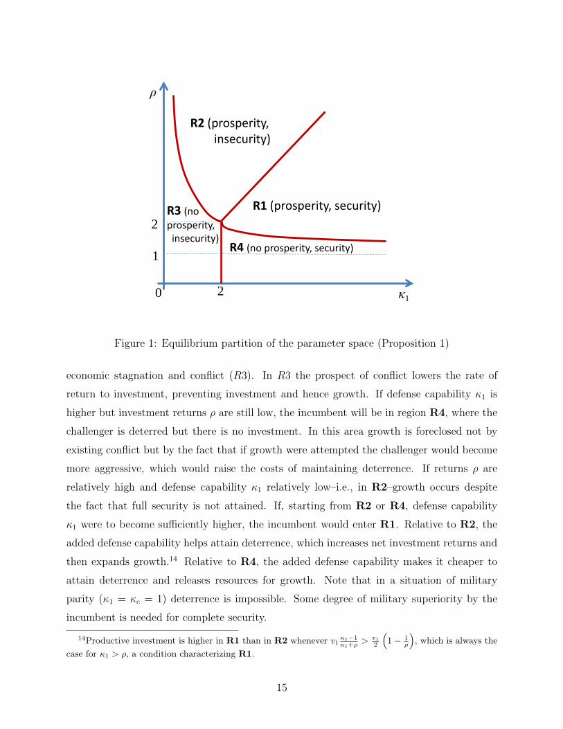
Figure 1: Equilibrium partition of the parameter space (Proposition 1)

economic stagnation and conflict (R3). In R3 the prospect of conflict lowers the rate of

return to investment, preventing investment and hence growth. If defense capability κ1 is

higher but investment returns ρ are still low, the incumbent will be in region R4, where the

challenger is deterred but there is no investment. In this area growth is foreclosed not by

existing conflict but by the fact that if growth were attempted the challenger would become

more aggressive, which would raise the costs of maintaining deterrence. If returns ρ are

relatively high and defense capability κ1 relatively low–i.e., in R2–growth occurs despite

the fact that full security is not attained. If, starting from R2 or R4, defense capability

κ1 were to become sufficiently higher, the incumbent would enter R1. Relative to R2, the

added defense capability helps attain deterrence, which increases net investment returns and

then expands growth.14 Relative to R4, the added defense capability makes it cheaper to

attain deterrence and releases resources for growth. Note that in a situation of military

parity (κ1 = κc = 1) deterrence is impossible. Some degree of military superiority by the

incumbent is needed for complete security.

14Productive investment is higher in R1 than in R2 whenever v1κ1−1κ1+ρ

> v12

(1− 1

ρ

), which is always the

case for κ1 > ρ, a condition characterizing R1.

15

Inspection of Figure 1 yields the following,

Remark 1 From a situation of no prosperity nor security (R3), a large enough increase in

defense capability κ1 is a necessary and sufficient condition for attaining both prosperity and

security; in contrast,

Remark 2 Increases in the growth capability ρ are not necessary nor sufficient for attaining

both security and prosperity.

Natural shocks could increase or decrease parameters like ρ and κ1. An incumbent that

enjoys security and prosperity in R1 could, through a reduction in κ1, be plunged into

stagnation and conflict in R3. A reduction in κ1 could be thought of as a negative shock to

the incumbent’s defense technology.

As said earlier, the (security, prosperity) regimes characterized in Proposition 1 are in-

variant in initial income v1; that is, whether investment i1 and arming by the challenger b1

are positive or zero does not depend on v1. But changes in income v1 do affect the particular

values of all endogenous variables whenever positive. In particular, we have the following,

Remark 3 Increases in initial income v1 exacerbate conflict; that is, in regimes where (ei-

ther or both) a1 and b1 are positive, they increase with v1.

Proof: see appendix.

This result highlights one of the central forces in the prosperity-security paradox, namely

the fact that a more productive incumbent that cannot fully deter its enemies will be engulfed

in more virulent conflict.

In order to connect the model to the historical record, we now relate the regions in

Figure 1 to the event of a civilization rising. We defined stateness as a relative high degree of

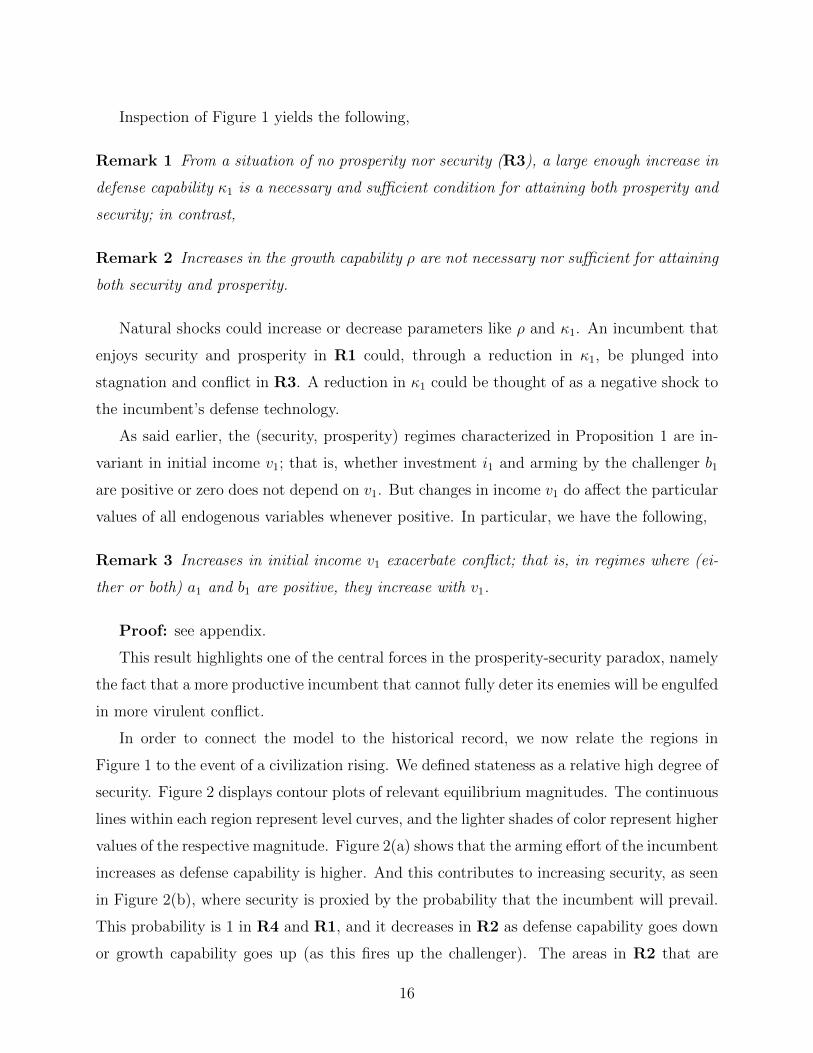
security. Figure 2 displays contour plots of relevant equilibrium magnitudes. The continuous

lines within each region represent level curves, and the lighter shades of color represent higher

values of the respective magnitude. Figure 2(a) shows that the arming effort of the incumbent

increases as defense capability is higher. And this contributes to increasing security, as seen

in Figure 2(b), where security is proxied by the probability that the incumbent will prevail.

This probability is 1 in R4 and R1, and it decreases in R2 as defense capability goes down

or growth capability goes up (as this fires up the challenger). The areas in R2 that are

16

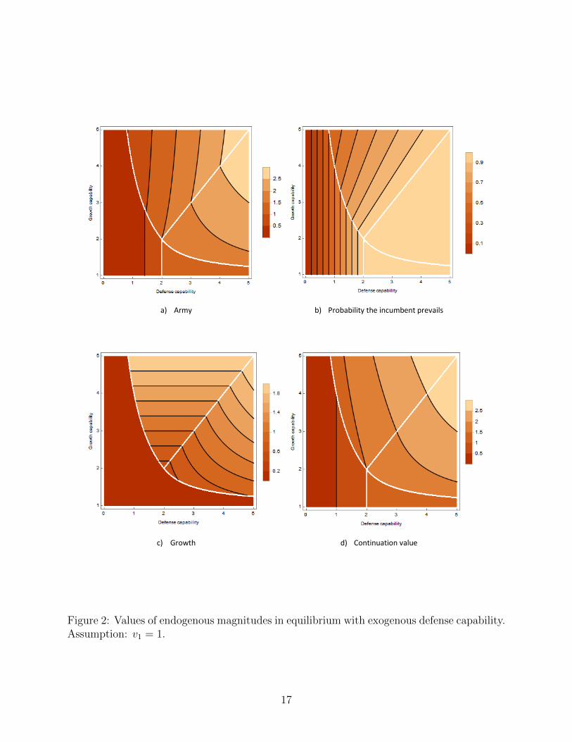
a) Army b) Probability the incumbent prevails

c) Growth d) Continuation value

Figure 2: Values of endogenous magnitudes in equilibrium with exogenous defense capability.Assumption: v1 = 1.

17

sufficiently close to R1 display very high levels of security (approaching full security where

R2 meets R1) which in our approach can be interpreted as a high degree of stateness.

In other words, we may consider R1 and the safer parts of R2 and R4 as the parameter

combinations that yield statehood. But civilization requires more than security; it also

requires the creation of surplus, which in our model amounts to growth (v2 − v1 = i1ρ).

Figure 2(c) shows how there is no growth in R3 and R4 (since there is no investment) and

that there is growth in R2 and R1. Growth increases with returns ρ and in R1 it also

increases with defense capability, as a higher defense capability lowers the costs of arming

and releases resources for investment. In R2 growth is unresponsive to defense capability

because any increase in κ1 is met with a similar increase in a1, which keeps the resources

devoted to defense a1κ1

and investment i1 constant.

We defined civilization as the joint attainment of growth and security. This would leave

out parts of R2 to the North-West, bordering R3, where growth can be high but security low.

This is sensible if we consider that civilization requires to consolidate growth by defending

production from attacks. A good proxy for civilization would then be the continuation value

perceived by the incumbent in period 1, which reflects both growth and security. This is the

expected future income of the incumbent resulting from investment and the probability that

the incumbent prevails. This combination of the magnitudes in panels (b) and (c) yields the

pattern in panel (d) of Figure 2. We observe that this “intersection” of growth and security

increases with both defense and growth capabilities, and indicates areas in R1 and R2 near

the 45 degree line as those that best escape the security-prosperity paradox, and therefore

as good parametric candidates for representing the rise of civilizations.

3.3 Discussion of modeling choices

Internal vs external conflict and social structure of incumbent polity The mod-

ern distinction between national and international conflict is irrelevant in our model. The

process of civilization emergence precedes such distinctions. That process ended with the

incorporation of the formerly hostile populations in some cases and their exclusion in oth-

ers. If challengers are internal actors (ex ante or ex post) our definition of security is about

internal order and the classic monopoly of violence. If challengers are external actors, our

definition of security is best matched with the notion of sovereignty. Second, there is no

18

distinction between ruler and subjects within the incumbent actor. The incumbent in our

model can be taken to be either a representative agent in the civilized center, a perfectly

benevolent ruler acting on behalf of that settled population, or a perfectly extractive ruler

who is a residual claimant.15

Asymmetries We have kept as many aspects as possible symmetric between the in-

cumbent and the challenger, and only introduced asymmetries that we deemed necessary to

analyze the type of interaction of interest. One asymmetry is that the incumbent acts as a

Stackelberg leader. This helps make deterrence possible. Another asymmetry is that while

defense effort costs the incumbent resources, it does not deplete a budget for the challenger.

This is for tractability. It would be possible to include a budget constraint for the chal-

lenger, and the advantage of a wealthier incumbent at being able to finance higher defense

effort, and then attaining deterrence, would operate in similar fashion. However, the reac-

tion function of the challenger would hit its constraint eventually and the analysis would

become less elegant as kinks in the reaction function would have to be taken into account.

A third asymmetry is that the incumbent can accumulate and the challenger does not. This

was both for tractability and to match the situation of historical interest, where one settled,

food-producing, group has more room to accumulate than rival nomadic groups.

Dynamic considerations Our model has two periods. Two natural questions arise,

namely (i) whether the same results can obtain in a static setting, and (ii) whether things

would change qualitatively if more periods, including possibly infinitely many, were consid-

ered. We now consider each question in turn.

(i) A static setting would not allow for investment and growth, but related tensions can

be explored between activities that yield no return (consumption) and others that yield some

return (production) but are perhaps more vulnerable to expropriation. However, in a static

model, either all resources are appropriable, or only production is. What a static model can-

not yield is a situation where as in our model baseline resources v are not appropriable now,

but are fully appropriable later if investment triggers an attack. This inherently dynamic

aspect matters for the partition result in Proposition 1.

15The latter interpretation is more suitable if growth in our model is interpreted in per capita terms,because extraction and concentration of surplus in a few hands would be a way in which an ancient societycould escape Malthusian population adjustment. Alternatively we can interpret growth in our model interms of per working capita, or at the level of groups, where wealth becomes population. We thank OdedGalor and David Weil for bringing these issues to our attention.

19

(ii) In the two period model, investment is deterred by the prospect of insecurity, and

since there is no conflict in period 2, there is no incentive to invest in period 1 and then use

the proceeds to mount a strong defense in period 2. This lack of stationarity is the essential

aspect one would hope to resolve in an infinite horizon model. While extending our model

to an infinite horizon has proven difficult, the key insight one would hope to obtain from

such an extension can be explored in a three period version, which we have solved. This

extension is a particular case of the model solved below for endogenous defense capabilities

and is available upon request. The question can be recast thus: does the presence of a third

period, and the projected need to fight in the future, eliminate the disincentives to invest

that arise from projected prosperity attracting predation? The answer is no. The key tension

between prosperity and security remains.

The use of contests Like many authors before us, we use contests and abstract from

bargaining and transfers. As is well known, even when transfers are possible inefficient

conflict may occur, for example due to inconsistent priors across players, agency issues, com-

mitment problems, or asymmetric information (see Jackson and Morelli (2011) for a survey

of reasons for war). Every paper on conflict must take a stand on whether to microfound the

breakout of conflict by reference to one of those phenomena or not. The cost of the added

microfoundation structure is justified when a specific distortion responsible for conflict is

particularly likely or germane given the problem under investigation. When the researcher

remains agnostic about such connections, the more parsimonious approach that we take

seems warranted.

4 Historical illustrations

4.1 Egypt and the birth of a state

Among the first civilizations, Egypt is the prototype of a “pristine territorial state,” the

undisputed pioneer in attaining both security and prosperity over an extended territory.

Although the Neolithic Revolution occurred in Egypt later than in Mesopotamia, the ensuing

process of social and political development in Egypt was faster.16 In less than a thousand

16During the Neolithic revolution, gathering and hunting were gradually replaced by the domesticationof plants and animals for food production. The process began in the ancient Near East (Southern Levant)about 10,000 years ago. The Neolithic in Egypt developed much later, around 5500 BC. According to Bard

20

years, the outcome would be a state that not only managed a relatively wealthy economy

but was also able to protect the surplus generated within it for long stretches of time. As

Allen (1997: 135) put it, “the Egyptian state lasted longer and was more stable than most

empires established elsewhere.”

Although the specific conditions underlying Egypt’s dual economic and political evolution

are disputed, a strong consensus exists around the idea that geography played a key role,

in the form of the Nile river and the surrounding desert. Our model can be used to assess

their role in explaining the emergence of a successful state by reference to our three deep

parameters, v1, ρ and κ1.

(1) The Nile river as a fundamental driver of the Egyptian economy. The Nile had at

least two key properties: a yearly flood that fertilized the soil with rich silt, and a two-way

navigability that facilitated exchange along the entire valley.17 “[T]he Nile was perfectly

ordered—its current carried boats downstream, the wind blew them back upstream—and the

Nile’s regular flooding renewed the fields and made farming so easy that in the Delta men

had ‘only to throw out seeds to reap a crop.’” (Bradford 2001: 9). Both properties, natural

fertility and easy exchange, map into a high v1 in our model, whereby initial income is high

even before investments are made.

(2) The growth potential of artificial irrigation. Egyptians could vastly increase their

economic output by investing in water management, which in the Nile valley took the form

of basin irrigation. Egyptians used a grid of basins to trap the floodwater and hold it for

much longer than it would naturally stay, vastly increasing soil fertility before planting.18

Economic sociologists agree that in Egypt irrigation agriculture “could generate crop-to-seed

yield of between 12:1 and 24:1 . . . but only at the cost of high capital investments” (Morris

and Manning 2005: 141). For Michael Mann, artificial irrigation was one of the earliest

(1994, p. 267), “The beginning of the First Dynasty was only about 1000 years after the earliest farmingvillages appeared on the Nile, so the Predynastic period, during the 4th millennium B.C., was one of fairlyrapid social and political evolution.”

17Most of the flow originated from monsoons in the Ethiopian highlands, and a smaller part came fromthe upper watershed of the White Nile around Lake Victoria. With impressive precision, the river began torise in the South in early July and the flood got to the Northern end of the valley by mid September. TheTigris and Euphrates were not only less predictable in timing, but also more irregular in volume.

18According to a long scholarly tradition (Weber [1909] 2013, Wittfogel 1957), water management andstate formation were closely linked in ancient societies. The thesis of “hydraulic empires,” which claims thatirrigation was a public good with enormous fixed costs, and that pristine states formed precisely in order toprovide them, has been discredited by evidence showing that irrigation was not preceded by the emergenceof state administrations.

21

forms of substantial economic investment, which in Egypt was even more profitable than

in Mesopotamia. Both in Egypt and Mesopotamia, irrigation agriculture could “generate

a surplus far greater than that known to populations on rain-watered soil” (1986: 80). In

Egypt, “the process was as in Mesopotamia, but squared,” and “as productivity grew, so too

did civilization, stratification, and the state” (1986: 108). In our model, a high value of the

parameter ρ reflects an environment in which investments yield large increases productivity

in the same way that the construction of irrigation systems resulted in major expansions of

food production in Egypt.

(3) Territorial isolation as natural protection. The Nile basin is surrounded by deserts,

which made invasions much less likely than in other food-producing centers. According to

Bradford (2001: 9), “The sea to the north and the deserts west and east isolated the Egyptians

from the rest of mankind, except for merchants, some infiltrators, and the occasional raid.”

The desert provided two kinds of protection. It discouraged the emergence and settlement

of hostile neighbors nearby, and acted as a barrier against distant rivals. In terms of our

model, Egypt’s territorial isolation maps into a naturally high κ1.

How do these conditions account for Egypt’s twin achievements of security and prosperity

in the context of our model? A high level of v1 has no effects in terms of which of the four

security-prosperity outcomes will arise, except that rivals, if present and belligerent (as in

R2 and R3), would become more aggressive. The implication is that the extraordinary soil

fertility along the Nile was not a favorable factor per se. In fact, highly productive soils are

not unique to Egypt. But the model does highlight that a combination of a high κ1 and

a high ρ could help Egypt attain prosperity and security. As just argued, the geography

afforded Egypt natural protection yielding a high κ1, and the potential for productivity-

enhancing irrigation offered a high ρ. In this context, Egyptian rulers had incentives to

promote investments that would increase future surplus, and could also defend it.

The resulting picture is one where Egypt is located in a favorable section of region R2, if

not directly in R1. The reason to place Egypt during the state formation period (end of the

Naqada II period, around 3200BC) in a good part of R2 is that Egypt did face occasional

attacks, and perhaps the total absence of challenges that characterizes R1 is better reserved

to the heights of Egyptian power under the New Kingdom, when the Egyptian state was

even more dominant than during its formative phase. A “good” part of R2 is one near the

frontier with R1, where conditional on ρ, κ1 is so high and the cost of defense effort by the

22

incumbent so small that victory is very likely. Thus, a society in such “good” part of R2

would grow and enjoy a relatively secure existence, because the probability of defeat is small,

and the returns to investment are high.

4.2 The end of the Bronze Age

For a period of almost 400 years, multiple states emerged in the Eastern Mediterranean

that improved their productive capacity and were capable–mainly due to fortified walls and

chariots–of defending their wealth against “barbarian” populations. This set of thriving

states included the city-ports of the Levant, the kingdoms of Anatolia, the Egyptian empire,

and the city-states of Mesopotamia and Cyprus. But suddenly a collapse epidemic swept

across the Eastern Mediterranean around 1200BC. As Eric Cline puts it (2014: 241), “...the

world as they had known it for more than three centuries collapsed and essentially vanished”.

According to Drews (1993: 3), “Altogether the end of the Bronze Age was arguably the worst

disaster in ancient history, even more calamitous than the collapse of the western Roman

Empire.”

A long debate on the causes behind the end of the Bronze Age has hypothesized earth-

quakes (Schaeffer 1948), droughts and famines (Carpenter 1968), internal rebellions (Zuck-

erman 2007 and Carpenter 1968), or innovations in military technology (Drews 1993).

The hypothesis of earthquakes has been discredited in the face of new archaeological

evidence showing that most urban destruction was caused not by natural forces but by

human attack. Hittites and Egyptians left unequivocal testimonies of attacks by the “Sea

Peoples,” as the Egyptians called them, a diverse array of intruders with different geographic

and ethnic origins (Sandars 1987). The same evidence challenges a pure internal rebellion

story. The possibility of invasions remains, but forces the question of what caused them in

the first place. Two hypotheses consistent with available evidence are:

(1) A severe change in climate, which caused draught and famines, and compelled pop-

ulations in the periphery to invade in search for food. Cities that were storehouses of grain

fell victim to “a final resort to violence by a drought sicken people” (Carpenter 1968: 69).19

(2) A revolution in the means of war, which tipped the military balance in favor of

19A recent paleobotany study confirms a substantial climate change around the time of the collapse thatcould have caused a famine (Langgut, Finkelstein, and Litt 2013). In the interpretation of these authors theshock may have caused internal rebellions rather than foreign invasions.

23

nomadic intruders. According to Drews (1998: 33), “the Catastrophe was the result of a new

style of warfare that appeared toward the end of the thirteen century BC, [which] opened up

new and frightening possibilities for various uncivilized populations that until that time had

been no cause of concern to the cities and kingdoms of the eastern Mediterranean”. What

were the changes introduced by the “uncivilized populations”? Chrissantos (2008: 11)

summarizes them: “these tribes developed better and lighter body armor, [. . . ] lighter and

smaller round shields, [and] revolutionary longer, stronger swords [. . . ] They also invented

a new weapon, the javelin, which could be used as a missile to hurl at an enemy. They

[managed to] overcome the civilizations’ chariot advantage [...] Once these tribes mastered

sea travel, no shore was too far for an attack. The failure of the chariot in the face of this

new warfare marks the beginning of the Bronze Age world’s collapse”.20

Our incumbent-challenger model is compatible with both hypotheses (acting over most

of the region or by causing invasions in critical sites). Consider the challenger’s valuation to

be parametrized as hv, and the challenger’s military capability κc. We can then distinguish

between two separate forces at play: the motivation behind invasion (h for hunger) versus

the effectiveness of the means to invade (κc). The historical debate has sometimes considered

changes in motivation and effectiveness as rival explanations. While h and κc capture sub-

stantively different forces, as discussed in Section 3 they are mathematically equivalent: both

affect the aggressiveness of the challenger at the margin. Therefore, studying the compara-

tive statics of κc can illuminate the role of both changes in the motivation and aggressiveness

of barbarians.

The parameter κc was assumed equal to 1 in the baseline model. We now consider a move

to κc > 1. How will the incumbent fare when facing a tougher challenger? In other words,

how does a higher κc affect the partition of the parameter space derived in Proposition 1?

The following proposition yields the answer.

Proposition 2 Optimal behavior by the incumbent yields a partition of the parameter space

(ρ, κ1, v1) ∈ (1,∞)× (0,∞)× R+ into four distinct regions:

20A climate shock and military innovation are not mutually incompatible causes and can be combinedunder the form of a “Perfect Storm” (Cline 2014: Chapter 5). Another recent explanation builds on theidea of “System Collapse:” since late Bronze Age societies were tightly connected through commerce, thefall of a few of them (for whatever cause) could seet off “domino” effects. This allows for the theoreticalpossibility that weather- and technology-induced invasions had devastated only a critical number of nodesin the interconnected Eastern Mediterranean, but eventually provoked a general collapse.

24

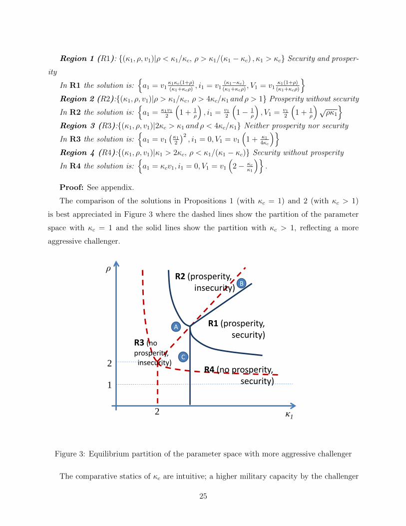
Region 1 (R1): {(κ1, ρ, v1)|ρ < κ1/κc, ρ > κ1/(κ1 − κc) , κ1 > κc} Security and prosper-

ity

In R1 the solution is:{a1 = v1

κ1κc(1+ρ)(κ1+κcρ)

, i1 = v1(κ1−κc)(κ1+κcρ)

, V1 = v1κ1(1+ρ)(κ1+κcρ)

}Region 2 (R2):{(κ1, ρ, v1)|ρ > κ1/κc, ρ > 4κc/κ1 and ρ > 1} Prosperity without security

In R2 the solution is:{a1 = κ1v1

2

(1 + 1

ρ

), i1 = v1

2

(1− 1

ρ

), V1 = v1

2

(1 + 1

ρ

)√ρκ1

}Region 3 (R3):{(κ1, ρ, v1)|2κc > κ1 and ρ < 4κc/κ1} Neither prosperity nor security

In R3 the solution is:{a1 = v1

(κ12

)2, i1 = 0, V1 = v1

(1 + κ1

4κc

)}Region 4 (R4):{(κ1, ρ, v1)|κ1 > 2κc, ρ < κ1/(κ1 − κc)} Security without prosperity

In R4 the solution is:{a1 = κcv1, i1 = 0, V1 = v1

(2− κc

κ1

)}.

Proof: See appendix.

The comparison of the solutions in Propositions 1 (with κc = 1) and 2 (with κc > 1)

is best appreciated in Figure 3 where the dashed lines show the partition of the parameter

space with κc = 1 and the solid lines show the partition with κc > 1, reflecting a more

aggressive challenger.

κ1

ρ

2

1 R4 (no prosperity, security)

2

R2 (prosperity, insecurity)

R3 (no prosperity, insecurity)

R1 (prosperity, security)

C

A

B

Figure 3: Equilibrium partition of the parameter space with more aggressive challenger

The comparative statics of κc are intuitive; a higher military capacity by the challenger

25

worsens outcomes in the following sense. For any point in the (κ1, ρ) space where either

security or prosperity (or both) are attained, a higher κc implies that security, prosperity

or both may be lost. A higher κc expands the area of all regions against R1 (where both

security and prosperity obtain). In addition, R3 which combined insecurity and stagnation,

grows at the expense of all others. A world with a more aggressive challenger is worse for

the incumbent.

The historical victory of the “Sea Peoples” over the kingdoms of the Ancient Near East

can be seen as a shift from the security-prosperity region (R1, or good parts of R2) to the

conflict-stagnation region (R3), as a result of positive shocks to the need that challengers

had to seize the economic output of the incumbent (an increase in h, in turn an effect of a

climatic change) or to the technology of attack (an increase in κc).

We can use the model to delve deeper into the diverging fates of different regions that

suffered attacks at the end of the Bronze Age. The extremes of that contrast are Egypt,

which managed to repel the invasion, and cities near the Mediterranean coast of the Levant,

like Ugarit, which were destroyed. In the case of Ugarit, surviving clay tablets provide

textual evidence on the threat of the Sea Peoples and the fact that Ugarit was defenseless.21

In terms of our model, Ugarit’s vulnerability at the time of the invasions can be interpreted

as either an initial location within R1 that was close to the vertex, and thereby not too far

away from R3, or within a narrow strip along the R2/R3 border on the side of R2. When

the shocks that prompted the invasion occurred the effect was to push Ugarit deep into R3.

In the new location, Ugarit faced the prospects of attacks that were too strong for the city

to resist. In the model, a deep position in R3 (closer to the ρ axis) entails a lower probability

that the incumbent will prevail. In fact, for Ugarit, the attack resulted in destruction.

Egypt was also a victim of barbarian attacks but the outcome was very different. Since

the end of the Second Intermediate Period, Egypt had developed a highly professional army

and a formidable fleet. Before the shock, Egypt was located deep in R1 so that the worst

effect of the shock could have been to relocate Egypt in a relatively safe neighborhood of

21In the tablets, Ammurapi, the king of Ugarit makes desperate requests to his Hittite overlord, whom headdresses as his “father” and who was using Ugarit’s maritime fleet to defend other sections of the Hittiteempire: “My father, behold, the enemy’s ships came (here); my cities(?) were burned, and they did evilthings in my country. Does not my father know that all my troops and chariots(?) are in the Land of Hatti,and all my ships are in the Land of Lukka?...Thus, the country is abandoned to itself. May my father knowit: the seven ships of the enemy that came here inflicted much damage upon us”. Letter RS 18.147 in JeanNougaryol et al. 1968. Ugaritica V, 24: 87–90. (Note: question marks in the original.)

26

R2. Egypt became susceptible to challenges, but it could prevail in the battlefield with

high probability. Pictorial inscriptions on the walls of the Karnak Temple attest to the

threats posed by the Sea Peoples at roughly the same time they invaded the Levant. But,

in contrast to Ugarit’s tablets, the Egyptian inscriptions actually honor king Merneptah’s

success in subduing the invaders. The contrasting cases of Ugarit and Egypt correspond

respectively to the points A or C and B in Figure 3.

The more general point resulting from our use of the model is to relate changes in deep

military and economic fundamentals to the arguments made by social theorists that the evo-

lution of political complexity is not unilinear, but plagued by dead ends and reversals. Ac-

cording to our model a shock to the fundamentals behind prosperity and security could cause

societies to lose either or both. The end of the Bronze Age involved state de-consolidation

and a regression to lower income levels—a Dark Age–, as in the region of conflict and stag-

nation, R3, in our model.

5 Endogenous defense capability and the transition to

security and prosperity

5.1 Setup

We will now allow the incumbent to spend resources in one period to increase its defense

capability in the next period. We introduce a period 0 before the periods 1 and 2, with the

incumbent facing a different challenger in each period. Since the challenger will never fight

in period 2, the incumbent will never spend in expanding defense capability in period 1.

Thus, the decision to augment defense capability will be relevant only in period 0. In period

0 the incumbent has a defense capability κ0, and can spend an amount m0 that will take

defense capability in the next period to κ1 = κ0 + γm0, where γ captures the purchasing

power of income in terms of defense means. We assume γ ∈(

0, 164+κ0

)where the upper

bound is a technical assumption to guarantee the possibility of partial transitions (where

either prosperity or security are attained but not both). To make things interesting, we

assume (κ0, ρ) are such that if things were left unchanged, in period 1 the incumbent would

find himself in region R3, which means he cannot expect growth nor security. In particular,

we impose the following,

27

Assumption 1 ρκ0 < 4 and κ0 < 2.

All other aspects of the interaction between challenger and incumbent remain as before,

and for simplicity we return to the case where κc = 1.

Timing In period 0, the incumbent starts by selecting m0. Then, in each period

t = 0, 1, 2 the incumbent selects at and it.22 After observing (m0, at, it) the challenger

selects bt. If bt = 0, the incumbent retains his position in the next period. If bt > 0, then

there is a war at the end of period t. The winner becomes the incumbent in the next period,

and faces a new challenger then.

Payoffs The fact that there is a new type of expenditure changes the incumbent’s

budget constraint to v0−m0− a0κ0− i0 ≥ 0. As before, we solve the model through backward

induction. The solution for periods 1 and 2 is given by our analysis in the previous section.

That analysis tells us the expected payoff for being an incumbent in period 1 is,

V1(i0,m0) = (v0 + ρi0)×

(κ0+γm0)(1+ρ)κ0+γm0+ρ

(κ0 + γm0, ρ) ∈ R1√(κ0+γm0)

ρ(1+ρ)

2(κ0 + γm0, ρ) ∈ R2(

1 + κ0+γm0

4

)(κ0 + γm0, ρ) ∈ R3(

2− 1κ0+γm0

)(κ0 + γm0, ρ) ∈ R4

≡ (v0 + ρi0)S(m0)

Given this continuation value, we can solve for decisions in period 0. After the incumbent

has selected m0, a0 and i0, the challenger decides whether to arm himself. Using the same

logic as in the previous section, we see that the challenger’s best response function is,

b0(a0,m0, i0) =

√a0V1(i0,m0)− a0 if a0 < V1(i0,m0)

0 if a0 ≥ V1(i0,m0)

This notation embeds the four regions over which V1(i0,m0) is defined into the calculus of

the challenger. Given this best response function, the incumbent has to choose a0, i0 after

he chose m0 such that the incumbent maximizes his expected utility:

22The assumption that m0 is decided before a0 and i0 is just to simplify the exposition. It is equivalentto assume that the incumbent selects all three variables simultaneously since the challenger does not moveuntil the incumbent has selected all of his actions. What is of course important is that the incumbent makeshis choices before the challenger.

28

maxa0,i0≥0

v0 −m0 −a0κ0− i0 +

a0a0 + b0(a0, i0,m0)

V1(i0,m0)

subject to the nonnegativity constraints a0 ≥ 0, i0 ≥ 0, the budget constraint v0−m0− a0κ0−

i0 ≥ 0 (BC) and the deterrence constraint (v0 + ρi0)S(m0)− a0 ≥ 0 (DC).

Notice this problem in period 1 is similar to the one with two periods in the previous

section, except now the continuation value depends explicitly on m0 (which is fixed at this

stage, given the convention that it was selected before a0 and i0) through S(m0). The

objective function is differentiable and concave in a0 and i0, the constraints are linear, so

the first order and complementary slackness conditions that are necessary and sufficient for

a maximum are,

a0 :1

2

√(v0 + ρi0)S(m0)

a0− 1

κ0− λBC

κ0− λND + λa = 0 (14)

i0 :ρ

2

√a0

(v0 + ρi0)S(m0)− 1− λBC + λNDρS(m0) + λi = 0 (15)

λBC(v0 −m0 −a0κ0− i0) = 0, λND ((v0 + ρi0)S(m0)− a0) = 0, λaa0 = 0, λii0 = 0 (16)

As before, λBC , λND are the Lagrange multipliers for the budget constraint and deterrence

constraints, and λa, λi are the multipliers for the non-negativity constraints for the control

variables.

5.2 Solution

Again the infinite marginal utility of a0 at zero implies a0 > 0 and λa = 0, so there are in

principle eight possible cases depending on whether the remaining three Lagrange multipliers

are positive or zero. A technical lemma that we prove as part of the next proposition

demonstrates that under our Assumption 1 there are only two feasible cases in period 0,

neither of which features productive investment. With this result, we can compute the

incumbent’s expected utility for any value of m0, and study his incentives to make changes

in defense capability.

29

To preview, the effect of m0 on the incumbent’s utility depends on the initial conditions

in period 0. If the maximum utility is attained for extremely low m0, then the incumbent

will remain stuck with insecurity and no prosperity (R3) in period 1. On the contrary, if

the optimal m0 is sufficiently high, security and prosperity will obtain in period 1. In other

words, the level of m0 can induce transitions from R3 to other regions in the next period, as

well as shift the optimal choices of a0 and i0. The key difficulty is that these shifts cause the

objective not to be everywhere differentiable nor concave in m0. Characterizing the optimum

requires examining the expected utility levels that obtain in the different cases (this lengthy

proof is relegated to the online appendix). We now establish,

Proposition 3 (a)Under Assumption 1 and provided that ρ < 2, there exist cutoffs τL, τM

and τH , τL < τM < τH such that:

1. If γv0 < τL, the polity stays in R3 (stagnation without security);

2. If τH < γv0, the polity moves to R1 (attains security and prosperity); and

3. If τM < γv0 < τH , the polity moves to R4 (attains security without prosperity)

(b) Under Assumption 1 and provided that ρ ≥ 2, there exist cutoffs σL, σM1, σM2 and

σH , satisfying σL < σM1 < σH and σL < σM2 < σH such that:

1. If γv0 < σL, the polity stays in R3 (stagnation and conflict);

2. If σH < γv0, the polity moves to R1 (attains security and prosperity); and

3. If σM1 < γv0 < σM2, the polity moves to R2 (attains prosperity without security)

This proposition tells us that, given the initial military capacity κ0 and the productivity

of investment ρ, the transitions followed by the polity will be very different depending on

the initial income γv0 in terms of defense capability purchasing power. If γv0 is very low,

the polity will remain trapped without security or prosperity. If γv0 lies in an intermediate

region, the polity can move into a region of partial achievement. If ρ < 2, the transition is to

R4 where it will attain peace but will not grow. The reason is that even though it attains a

higher defense capability κ1 in the next period, which gives the incumbent the ability to fend

off attacks at a lower cost, the benefit from consumption will still be higher than the present

value from investing. If ρ > 2, the “hybrid” transition is to R2 where it will grow without

attaining full security (proving the existence of bounds σM1, σM2 for this transition makes

use of our technical assumption γ ∈(

0, 164+κ0

)). If γv0 is very high, however, the subsequent

30

military capacity κ1 will allow the incumbent to free resources for both a deterrent army

and a large-scale investment at R1.

To summarize, while large enough initial income (or cheap enough defense capability)

guarantees security and prosperity through sufficient accumulation of defense capability,

intermediate levels may only allow to attain either security or prosperity. The Hobbesian

argument that security is a precondition for prosperity is qualified in this model. Baseline

prosperity can buy defense capability, and only then can the ensuing security promote more

prosperity.

6 Historical Illustration: Sumeria and the origin of civ-

ilization

Southern Mesopotamia was the source of the first substantial surplus in human evolution,

and the area where the first city-states formed, giving rise to the first major civilization. A

riverine valley along the Tigris and Euphrates, exceptionally endowed for alluvial agricul-

ture, was the key for economic prosperity. Like in Egypt, Southern Mesopotamians made

massive investments in the creation of irrigation infrastructure, securing extraordinary re-

turns. According to Mann (1986: 78), “If [the alluvium] can be diverted onto a broad area of

existing land, then much higher crop yields can be expected. This is the significance of irri-

gation in the ancient world: the spreading of water and silt over the land. Rain-watered soils

gave lower yields.” Liverani (2005, p. 5) offers an idea of the increase in yields that could

be obtained: “The agricultural production of barley underwent a notable, possibly tenfold,

increase thanks to the construction of water reservoirs and irrigation canals, of long fields

adjacent to the canals watered by them, and thanks to the use of the plow, of animal power,

of carts, of threshing sledges, of clay sickles, and of improved storage facilities.”

These high returns to productive investment help place Sumeria in the parameter space

of our model as a case of high ρ. But what about the other parameter, the defense capability

κ1? In contrast to Egypt, geography did not afford the Sumerians natural protection against

attacks. On the contrary, the natural landscape exposed Sumeria to numerous threats. As

Bradford (1993: 4) puts it, “Their neighbors to the west, the Amorites, nomads of the desert,

infiltrated Mesopotamia... The neighbors to the east, who dwelled in the mountains, were the

31

Gutians and the Elamites. The Gutians and, to a lesser extent, the Elamites considered

Sumer and Akkad a treasurehouse to be raided”. Finer (1997: 102) also emphasized the

porousness of the Sumerian frontiers.

In terms of our model, the vulnerability of Sumeria to invaders means that defense

capability κ0 was low. Given a low κ0, Sumeria’s trajectory must have begun in the conflict-

stagnation region, R3. But if output was so insecure, how could the first human civilization

emerge at all? That is, how did Sumerians solve the problem of protecting surpluses from

raiders and encouraging investments in productive infrastructure?

The extended model featuring endogenous defense capability provides an answer. Our

proposition 3 states that an incumbent that is initially in R3 due to a low defense capability

κ0, may invest in defense capability in order to attain sufficient security against the chal-

lenger. The key condition for this investment to be undertaken is for initial productivity v0

to be high enough. The archaeological record suggests Sumeria was well placed to meet that

requirement. The availability of alluvial agriculture combined with an unparalleled initial

endowment of plant and animal domesticates furnished the entire Fertile Crescent with ex-

ceptional advantages. It is well known that due to altitude and climatic variation, the Fertile

Crescent hosted a wide variety of plants with high potential for food production as well as

domesticable animals.23 According to Trigger (2003: 281), domesticated animals afforded

large gains in agricultural labor productivity, and may help explain why Sumeria and Egypt

were the first areas in the world to develop civilization. Given the natural advantages, Dia-

mond (1997: 135) claims that “any attempt to understand the origins of the modern world

must come to grips with the question why the Fertile Crescent’s domesticate plants and an-

imals gave it such a potent head start”. In terms of our model, this combination of initial

advantages can be captured by a high v0.

What is delicate about the role of the Fertile Crescent’s initial advantages is that a

high v0 can encourage predation by outside challengers. However, a high v0 could also help

finance the investments in defense that were needed to escape the conflict-stagnation trap

represented by region R3. It is by no means obvious that the “defense-financing” force

should dominate the predation force. This tension has a resolution in our model: for v0 low

23Diamond (1997: Ch. 8) highlights that all eight founder crops in the Neolithic were present in the area;in addition, out of the five most important domesticated animals, four were available in the Fertile Crescent(pigs, cows, sheep and goats).

32

enough, no escape from R3 is possible. For v0 high enough, the incentive to finance defensive

capabilities dominates. When defense is upgraded, security rises and ushers in productive

investments and growth. Figure A1 in the Online Appendix shows the comparison of the

cases of Egypt and Sumeria in terms of our parameter space (ρ, κ1): Egypt started in a good

region with relatively high levels of both parameters. Sumeria started with a low level of κ0

and it was through investment that it raised its defense capability to a higher κ1 that could

deliver sufficient security.

What is the evidence of endogenous defense capabilities in Sumeria? The archaeological

record offers evidence of large and generalized investments to improve defense in the form

of protective perimeter walls, which made Sumerian cities large-scale fortifications. Figure

A2 in the Online Appendix includes illustrations of four Sumerian cities. All of them had

walls. In fact, virtually every city in ancient history had walls. Walls were the endogenous,

artificial substitute for the missing natural protection that was present in Egypt (where cities

did not have walls).24

7 Conclusion

We build a model to investigate the combined operation of productive and defense capabil-

ities in a society where an incumbent seeks to consolidate security and grow the economy.

The components of the model are chosen by reference to the anthropological and histori-

cal literature, in order to capture relevant environmental parameters and the minimalistic

strategic dilemma facing proto-civilizations. States and civilizations arose together, and

therefore stateness, defined as a high degree of security, had to emerge in association with

the prosperity that tended to undermine it.

In elucidating the requirements for escaping the paradox, our model helps evaluate claims

about the relative role of security and prosperity that are central to classic theories of state

formation. We show that all four combinations involving the presence or absence of security

24According to van de Mieroop’s (1997) study of Mesopotamian cities, “Perhaps the presence of wallswas the main characteristic of a city in the eyes of an ancient Mesopotamian.” The archaeological recordsubstantiates not only the generalized presence of defense investments in rising city-states, but also theircostliness, which would have been prohibitive to societies with low initial productivity. Both walls and theoften complementary moats have been estimated to involve large investments (e.g., the cost estimate for themoat in the Babylonian city of Dur-Jakin is ten thousand men working for three and a half months (Van deMieroop, p. 76)).

33

and prosperity are possible, preventing simple characterizations of security or prosperity

being necessary or sufficient conditions for one another. These combinations match various

historical experiences of societies that attained neither, one, or both objectives. The key

implication of our theory is that a balance between productive and defense capabilities is

important in order to prevent a security breakdown and promote prosperity. History offers

examples of how naturally occurring high levels of productivity and defense, as in Egypt,

enabled the emergence of civilization. But it also offers examples of negative shocks that

destroyed civilizations, as in the end of the Bronze Age, which the model helps rationalize.

The extended model with endogenous defense capabilities explains how areas without natural

defense could, if productive enough, transition into security with prosperity and resolve the

civilizational paradox. The possibility of improving defense helps create the conditions where

productive investments can eventually be made without triggering predatory challenges.

This result may also help rationalize historical experiences where a temporary economic

boom allows the state to consolidate its power and usher in a phase of more sustained

growth. Isolating formally the pivotal role of defense capability to the civilizational process

contributes to the demanding enterprise of discerning how economic shocks can hinder or

help state formation and political stability more generally.

8 Appendix

Proof of Proposition 1: This is a particular case of the model with general values of κc,

which is studied in Proposition 2.

Proof of Remark 3: That a1 increases in v1 in all regimes follows directly from in-

spection of the solution for a1 in each regime in Proposition 1. To see that whenever pos-

itive b1 also increases in v1, take the value of b1 from the best response expression (4),

and substitute in the values of i1, a1 in regions R2 and R3. This yields respectively,

b1,R2 = v1

{√κ12

(1 + 1

ρ

)(1 + ρκ1−1

κ1+ρ

)− κ1

2

(1 + 1

ρ

)}and b1,R3 = v1

(κ12

) {1− κ1

2

}, which

are both positive and increasing in v1.�

34

Proof of Proposition 2: The problem is to maximize,

L = v1 −a1κ1− i1 +

a1a1 + b1

(v1 + ρi1)

+λBC(v1 −a1κ1− i1) + λDC(κcv1 − a1 + κcρi1) + λaa1 + λii1. (17)

We characterize the solution (a1, i1, λBC , λDC , λa, λi) to this problem for each parameter

combination (ρ, κ1, κc, v1). To save on notation, let us define PS = {(κ1, κc, ρ, v1)|κ1, κc >0, ρ > 1, v1 > 0} the parameter space we consider throughout the proof. The first order and

complementary slackness conditions that characterize the optimum are given by,

∂L∂a1

=1

2√κc

√v1 + ρi1a1

− 1

κ1− λBC

κ1− λDC + λa = 0; a1 ≥ 0, λa ≥ 0, λaa1 = 0 c.s. (18)

∂L∂i1

=ρ

2√κc

√a1

v1 + ρi1− 1− λBC + λDCκcρ+ λi = 0; i1 ≥ 0, λi ≥ 0, λii1 = 0 c.s. (19)

λBC(v1 −a1κ1− i1) = 0 c.s., λDC (κcv1 − a1 + κcρi1) = 0 c.s. (20)

Since λa = 0, there are eight possible cases to be analyzed, given by whether the remaining

Lagrange multipliers λBC , λDC , and λi are zero or positive. We will assume in each case that

the conditions defining it hold, and then determine which part if any of the parameter space

supports a solution. When the case implies conditions for the parameters that are mutually

exclusive, the case will be deemed infeasible. When the case implies that the solution can

be supported for knife-edge combinations of the parameter values (i.e., combinations that,

under a suitable measure, would have measure zero) we consider the case to be non-generic

and also drop it from further consideration.

1. Case λBC > 0 (BC binds), λDC > 0 (DC binds, consolidation), and λi = 0

(i1 > 0) Since a1 is always positive, and in this case i1 is also positive, the FOCs in (18),

(19) must hold with equality. Because this case involves binding BC and DC constraints,

35

they also hold with equality. This is,

a1 :1

2√κc

√1

κc− 1

κ1− λBC

κ1− λDC = 0; i1 :

ρ

2√κc

√κc − 1− λBC + λDCρκc = 0

DC : κcv1 − a1 + κcρi1 = 0; BC : v1 −a1κ1− i1 = 0,

implying that investment and army are i1 = v1(κ1−κc)(κ1+κcρ)

and a1 = v1κ1κc(1+ρ)(κ1+κcρ)

, respectively.

As a result λi = 0 (or i1 > 0) is supported by κ1 > κc. Using the FOCs, λDC > 0 ⇔κ1 > ρκc and λBC > 0 ⇔ ρ > κ1/(κ1 − κc). The parameter set supporting this solution

is R1 = {(κ1, ρ, v1) ∈ PS|ρ < κ1/κc, ρ > κ1/(κ1 − κc), κ1 > κc} and in this region there is

investment and deterrence. The expected utility is V1 = v1κ1(1+ρ)(κ1+κcρ)

. When κc > κ1, this case

would be infeasible, as it contradicts i1 > 0.

2. Case λBC > 0 (BC binds),λDC = 0 (DC does not bind, conflict), and λi = 0

(i > 0) The first order and complementary slackness conditions yield

a1 :1

2√κc

√v1 + ρi1a1

− 1

κ1− λBC

κ1= 0; i1 :

ρ

2√κc

√a1

v1 + ρi1− 1− λBC = 0

BC : v1 −a1κ1− i1 = 0

Investment and army solutions are respectively i1 = v12

(1− 1

ρ

)and a1 = κ1v1

2

(1 + 1

ρ

).

This solution is consistent with λDC = 0 (DC holds with strict inequality) and λi = 0 ⇔ρ > κ1

κcand ρ > 1 respectively. The solution is consistent with λBC > 0 ⇔ ρ > 4κc

κ1

(from checking λBC > 0 in the FOCs). As a result, the parameter set supporting this case

is R2 = {(κ1, ρ, v1) ∈ PS|ρ > κ1/κc, ρ > 4κc/κ1 } . Expected utility for the incumbent is

V1 = v12

(1 + 1

ρ

)√ρκ1.

3. Case λBC = 0 (BC does not bind), λDC = 0 (DC does not bind, conflict),

and λi = 0 (i1 > 0) Non-generic, since it is consistent for subset of the space (ρ, κ1, v1)

that has measure zero. This follows from (18) and (19), so when λBC , λDC , λi = 0, a1 :

12√κc

√v1+ρi1a1− 1

κ1= 0 and i1 : ρ

2√κc

√a1

v1+ρi1− 1 = 0. The first FOC implies

√v1+ρi1a1

=2√κc

κ1

and substituting into the second FOC, we get ρ2√κc

κ12√κc

= 1 or ρκ14κc

= 1, which implies this

holds for a non-generic parameter set.

4. Case λBC = 0 (BC does not bind),λDC > 0 (DC binds, consolidation), and

36

λi = 0 (i1 > 0) The FOCs are,

a1 :1

2√κc

√v1 + ρi1a1

− 1

κ1− λDC = 0; i1 :

ρ

2√κc

√a1

v1 + ρi1− 1 + κcρλDC = 0,

where a1 = κc (v1 + ρi1) indicating that λDC must simultaneously equal 12κc− 1

κ1and

( ρ2−1)κcρ

,

which forces the equality ρ = κ1κc

, which is non-generic.

5. Case λBC > 0 (BC binds), λDC > 0 (DC binds, deterrence), and λi > 0

(i1 = 0) Because i1 = 0, BC binding implies that a1 = κ1v1, but DC binding implies that

a1 = κcv1, so κ1 = κc which is non-generic.

6. Case λBC > 0 (BC binds), λDC = 0 (DC does not bind, conflict), and λi > 0

(i1 = 0) The BC binding and i1 = 0 yield a1 = v1κ1. The BC binds iff κ1 > 4κc. The DC

not binding, however, implies v1κc − v1κ1 > 0 ⇔ κc > κ1 which violates the condition for

BC to bind κ1 > 4κc, making this case infeasible.

7. Case λBC = 0 (BC does not bind), λDC = 0 (DC does not bind, conflict),

and λi > 0 (i1 = 0) In this case a1 = v1κ21/(4κc) and i1 = 0. This solution is consistent

with λBC = 0 and λDC = 0 ⇔ κ1 < 2κc. Also for λi > 0 we need 1 − ρκ1/(4κc) > 0 (from

the FOC of i1). Thus, this holds for any triple (ρ, κ1, v1) ∈ PS such that κ1 < 2κc and

ρ < 4κc/κ1. In other words, the parameter set for which this region contains the solution to

the incumbent’s problem is R3 = {(κ1, ρ, v1) ∈ PS|2κc > κ1, ρ < 4κc/κ1} . Expected utility

in this case is given by V1 = v1

(1 + κ1

4κc

).

8. Case λBC = 0 (BC does not bind), λDC > 0 (DC binds, consolidation),and

λi > 0 (i1 = 0) In this case the system of conditions is given by a1 : 12κc− 1

κ1− λDC = 0;

i1 : ρ2− 1 + λDCρκc + λi = 0; and BC : κcv1 − a1 = 0. Since i1 = 0, the DC yields

a1 = κcv1. For this to be consistent with λDC > 0, we must have from the first equation

that κ1 > 2κc, and to be consistent with λi > 0 we need ρ < κ1/(κ1 − κc), yielding R4 =

{(κ1, ρ, v1) ∈ PS|κ1 > 2κc, ρ < κ1/(κ1 − κc)} . The expected utility is V1 = v1

(2− κc

κ1

). �

References

Acemoglu, D., S. Johnson, and J. Robinson (2005). Institutions as a fundamental cause oflong-run growth. Handbook of economic growth 1 (2005): 385-472.

Allen, R. C. (1997), Agriculture and the Origins of the State in Ancient Egypt. Explorationsin Economic History 34, 135-54.

37

Bard, K. (1994), The Egyptian Predynastic: A Review of the Evidence, Journal of FieldArchaeology 21, 265–288.

Bates, R. (2001), Prosperity and violence: the political economy of development. NewYork: WW Norton.

Besley, T. and T. Persson (2011), Pillars of Prosperity: The Political Economics of Develop-ment Clusters: The Political Economics of Development Clusters. Princeton UniversityPress.

Boix, C. (2015), Political order and inequality: Their foundations and their consequencesfor human welfare. Cambridge University Press.

Bradford, A. (2001), With Arrow, Sword, and Spear. A History of Warfare in the AncientWorld. Westport, Connecticut and London: Praeger.

Carneiro, R. (1970). A Theory of the Origin of the State. Science 169 (3947): 733–738.

Carpenter, R. (1968), Discontinuity in Greek Civilization. New York: W. W. Norton & Co.

Childe, V. G. (1936), Man Makes Himself. London: Watts Publishers.

Chrissanthos, S. (2008), Warfare un the Ancient World. From the Bronze Age to the Fallof Rome. Westport, Connecticut and London: Praeger.

Claessen, H. and P. Skalnik (1978), The Early State. The Hague: Mouton Publishers.

Cline, E. (2014), 1177 BC - The Year Civilization Collapsed. Princeton, NJ: PrincetonUniversity Press.

Collier P. and A. Hoeffler (1998), On Economic Causes of Civil War, Oxford EconomicPapers 50, 563-73.

Diamond, J. (1999), Guns, Germs, and Steel: The Fates of Human Societies. WW Norton& Company.

Di Giacomo, G. and G. Scardozzi (2012), Multitemporal High-Resolution Satellite Imagesfor the Study and Monitoring of an Ancient Mesopotamian City and its SurroundingLandscape: The Case of Ur. International Journal of Geophysics,, Vol. 2012, ArticleID 716296.

Drews, R. (1993), The End of the Bronze Age. Changes in Warfare and the Catastropheca. 1200BC. Princeton, NJ: Princeton University Press.

Dube, O. and J.F. Vargas (2006), Are All Resources Cursed? Coffee, Oil and ArmedConflict in Colombia, mimeo Harvard University.

Fried, M. (1960), On the evolution of social stratificiation and the state. Indianapolis:Bobbs-Merrill.

38

Fritz, V. (1997), Cities: Cities of the Bronze and Iron Age, in Eric M. Meyers (ed.), TheOxford Encyclopedia of Archeology in the Near East, Vol. II, Oxford and New York,Oxford University Press, 19-25.

Garfinkel, M. and S. Skaperdas (2007), Economics of Conflict: An Overview, in T. Sandlerand K. Hartley (eds.), Handbook of Defense Economics, Vol. II, 649-709

Garfinkle, S. (2013), Ancient Near Eastern City-States. In Peter F. Bang and WalterScheidel (eds.), The Oxford Handbook of the State in the Ancient Near East andMediterranean. New York, Oxford University Press: 94-119.

Gennaioli, N. and H-J. Voth (2015). State capacity and military conflict. The Review ofEconomic Studies

Gibson, McG. (1993), Nippur – Sacred City of Enlil, Al-Rafidan: Journal of Western AsiaticStudies vol. XIV.

Grossman, H. and M. Kim (1995). Swords or Plowshares? A Theory of the Security ofClaims to Property. Journal of Political Economy 103(6), 1275-88.

Hawkes, J. (1974), Eridu, Iraq. Sumerian city circa 5000 B.C. Atlas of Ancient Archaeology.New York. McGraw-Hill Book Company.

Hirshleifer, J. (1991). The Paradox of Power. Economics & Politics 3(3), 177-200.

Jackson, M. and M. Morelli (2011). The Reasons for Wars: An Updated Survey. In: C.Coyne and R. Mathers (eds.), The Handbook on the Political Economy of War, EdwardElgar Publishing, chapter 3.

Johnson, A. and T. Earle (2000). The evolution of human societies: from foraging groupto agrarian state. Stanford University Press.

Jordan, J. (1931), Abhandlungen der Preussischen Akademie der Wissenschaften, Philosophisch-historische Klasse, Jahrgang 1930, Nr. 4.

Keeley, L. (1996), War before civilization: The myth of the peaceful savage. Oxford Uni-versity Press.

Langutt, D., I. Finkelstein, and T. Litt. 2013. Climate and the Late Bronze Collapse: NewEvidence from the Southern Levant, Tel Aviv, Vol. 40, 2013, 149–175.

Mann, M. (1986), The Sources of Social Power Vol. I: A history of power from the beginningto A.D. 1760. Cambridge University Press.

Mayshar, J., O. Moav, and Z. Neeman (2013). Geography, transparency and institutions.Mimeo University of Warwick.

Mayshar, J., O. Moav, Z. Neeman and L. Pascali (2015). Cereals, Appropriability andHierarchy. CEPR Discussion Paper 10742.

39

McNeill, W. (1982), The Pursuit of Power: Technology, Armed Force, and Society sinceA.D. 1000. University of Chicago Press.

Morris, I. and J. Manning (2005), The economic sociology of the ancient world, The Hand-book of Economic Sociology, 2d. ed. Eds. Neil Smelser & Richard Swedberg., Prince-ton: Princeton University Press, 131-159.

North, D., and B. Weingast (1989). Constitutions and commitment: the evolution ofinstitutions governing public choice in seventeenth-century England. The Journal ofEconomic History 49(4), 803-832.

Olson, M. (2000). Power And Prosperity: Outgrowing Communist And Capitalist Dicta-torships. Basic Books.

Powell, R. (2012). Persistent Fighting and Shifting Power, American Journal of PoliticalScience (2012) 56(3), 620-37.

Powell, R. (2013). Monopolizing Violence and Consolidating Power, Quarterly Journal ofEconomics 128 (2), 807-859

Ross, M. (2003). The Natural Resource Curse: How Wealth Can Make You Poor, in Collier,P. and I. Bannon (eds.) Natural Resources and Violent Conflict. The World Bank.

Sandars, N.K. (1987). The Sea Peoples: Warriors of the ancient Mediterranean, RevisedEdition. London: Thames and Hudson.

Schaeffer, C.F.A. (1948). Stratigraphie comparee et chronologie de l’Asie occidentale. Lon-don: Oxford University Press.

Spruyt, H. (1996). The sovereign state and its competitors: an analysis of systems change.Princeton University Press.

Tilly, Ch. (1975). The formation of national states in Western Europe. Vol. 8. PrincetonUniv Press.

Tilly, Ch. (1992). Coercion, capital, and European states, AD 990-1992. Oxford: Blackwell.

Trigger, B. (2003). Understanding early civilizations. Cambridge University Press.

Van de Mieroop, M. (1997). The ancient Mesopotamian city. Oxford University Press.

Weber, M. (1978). Economy and society. Berkeley, CA: California University Press.

Weber, M. (2013) [1909]. The agrarian sociology of ancient civilizations. London: VersoBooks.

Wittfogel, K. A. (1957). Oriental Despotism. New Haven: Yale Univ. Press.

Zuckerman, S. (2007). Anatomy of a Destruction: Crisis Architecture, Termination Ritualsand the Fall of Canaanite Hazor. Journal of Mediterranean Archaeology 20, 1: 3–32.

40

Online Appendix to The Paradox of Civilization

Ernesto Dal Bo

UC Berkeley

Pablo Hernandez-Lagos

NYU Abu Dhabi

Sebastian Mazzuca

Johns Hopkins

July 23, 2016

1

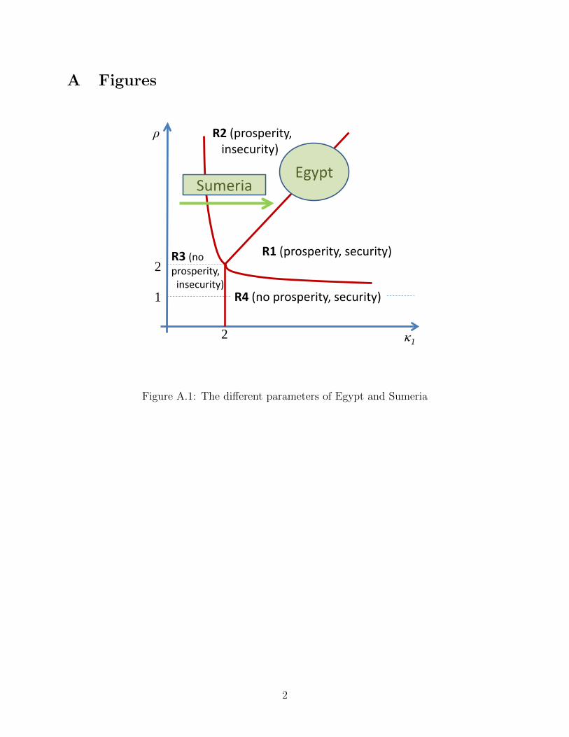
A Figures

κ1

ρ

2

1 R4 (no prosperity, security)

2

R1 (prosperity, security)

R2 (prosperity, insecurity)

R3 (no prosperity, insecurity)

Egypt Sumeria

Figure A.1: The different parameters of Egypt and Sumeria

2

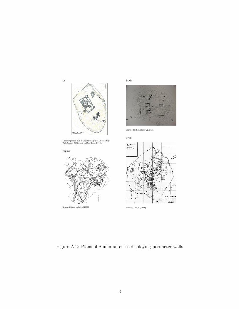
Ur

The new general plan of Ur (drawn up by F. Ghio): 1: City Wall. Source: Di Giacomo and Scardozzi (2012). Nippur

Source: Gibson, McGuire (1993).

Eridu

Source: Hawkes, J. (1974, p. 171). Uruk

Source: J. Jordan (1931).

Figure A.2: Plans of Sumerian cities displaying perimeter walls

3

B Proofs

Proof of Proposition 3: Before analyzing the choices of m0, we narrow down the possible

equilibrium choices of a0 and i0. The following Lemma shows that given our Assumption 1

there are only two feasible cases in period 0.

Lemma 1 If Assumption 1 holds, then in period 0 the incumbent chooses:

i) i0 = 0 and a0 =κ204v0S(m0) when v0S(m0)

(v0−m0)< 4

κ0; or

ii) i0 = 0 and a0 = κ0(v0 −m0) when v0S(m0)(v0−m0)

> 4κ0.

Proof of lemma 1: There are two cases that constitute a solution out of eight possible

ones. We will show that the assumption 1 implies that the first case holds when v0S(m0)v0−m0

< 4κ0

and the second case holds when v0S(m0)v0−m0

> 4κ0

. The remaining six cases can be shown to be

either inconsistent with any set of parameter values or consistent only with a non-generic

set.

1. Case λBC = 0 (BC does not bind),λND = 0 (DC does not bind, conflict),

and λi > 0 (i0 = 0)

The FOCs are,

a0 :1

2

√v0S(m0)

a0

− 1

κ0

= 0 (1)

i0 :ρ

2

√a0

v0S(m0)− 1 + λi = 0 (2)

This implies,

a0 =κ2

0

4v0S(m0)

4

λi = 1− ρκ0

4

The necessary and sufficient conditions for this case to hold are,

λBC = 0⇔ v0S(m0)

v0 −m0

<4

κ0

(from the BC not binding)

λDC = 0⇔ 1 >κ2

0

4⇔ κ0 < 2 (from the DC not binding)

λi > 0⇔ 1− ρκ0

4> 0⇔ ρ <

4

κ0

(from the FOC for i0)

The first inequality holds for values of m0 low enough given κ0 < 2, and the second and

third hold by assumption 1.

2. Case λBC > 0 (BC binds),λDC = 0 (DC does not bind, conflict), and λi > 0

(i0 = 0)

The FOCs are,

a0 :1

2

√v0S(m0)

a0

− 1

κ0

− λBCκ0

= 0 (3)

i0 =ρ

2

√a0

v0S(m0)− 1− λBC + λi = 0 (4)

λBC > 0 implies κ0 (v0 −m0) = a0.

From the FOCs, we obtain,

λBC =κ0

2

√v0S(m0)

a0

− 1

λi =κ0

2

√v0S(m0)

a0

− ρ

2

√a0

v0S(m0).

5

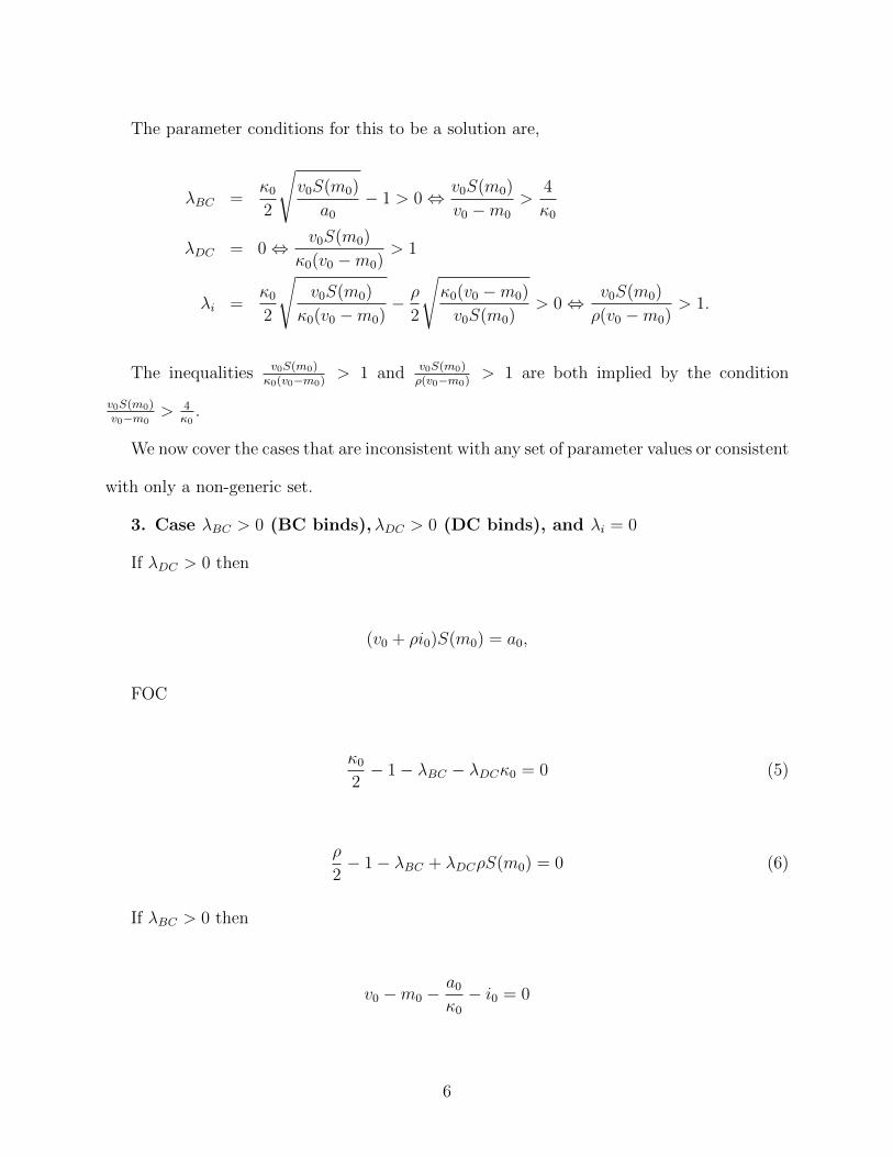
The parameter conditions for this to be a solution are,

λBC =κ0

2

√v0S(m0)

a0

− 1 > 0⇔ v0S(m0)

v0 −m0

>4

κ0

λDC = 0⇔ v0S(m0)

κ0(v0 −m0)> 1

λi =κ0

2

√v0S(m0)

κ0(v0 −m0)− ρ

2

√κ0(v0 −m0)

v0S(m0)> 0⇔ v0S(m0)

ρ(v0 −m0)> 1.

The inequalities v0S(m0)κ0(v0−m0)

> 1 and v0S(m0)ρ(v0−m0)

> 1 are both implied by the condition

v0S(m0)v0−m0

> 4κ0

.

We now cover the cases that are inconsistent with any set of parameter values or consistent

with only a non-generic set.

3. Case λBC > 0 (BC binds),λDC > 0 (DC binds), and λi = 0

If λDC > 0 then

(v0 + ρi0)S(m0) = a0,

FOC

κ0

2− 1− λBC − λDCκ0 = 0 (5)

ρ

2− 1− λBC + λDCρS(m0) = 0 (6)

If λBC > 0 then

v0 −m0 −a0

κ0

− i0 = 0

6

We have four equations and four unknowns. Therefore

λDC =1

2

(κ0 − ρ

κ0 + ρS(m0)

)

λBC =ρ

2

(κ0 + κ0S(m0)

κ0 + ρS(m0)

)− 1

i0 =v0κ0 −m0κ0 − v0S(m0)

κ0 + ρS(m0)

a0 =

(v0κ0 (1 + ρ)− ρm0κ0

κ0 + ρS(m0)

)S(m0)

We need to establish the conditions on the parameters and m0 such that those parameters

support this equilibrium.

λDC =1

2

(κ0 − ρ

κ0 + ρS(m0)

)> 0 ⇐⇒ κ0 > ρ

λBC =ρκ0

2

(1 + S(m0)

κ0 + ρS(m0)

)− 1 > 0 ⇐⇒ ρ >

2κ0

κ0 (1 + S(m0))− 2S(m0)

⇐⇒ S(m0)(κ0

2− 1)>κ0

ρ− κ0

2.

The LHS of this inequality is positive since from above λDC > 0 ⇐⇒ κ0 > ρ and by

assumption κ0 < 2. This last assumption also implies the RHS is negative, so the inequality

can never hold and this case can never occur.

4. Case λBC > 0 (BC binds),λDC = 0 (DC does not bind, conflict), and λi = 0

(i0 > 0)

7

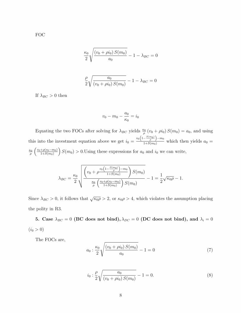
FOC

κ0

2

√(v0 + ρi0)S(m0)

a0

− 1− λBC = 0

ρ

2

√a0

(v0 + ρi0)S(m0)− 1− λBC = 0

If λBC > 0 then

v0 −m0 −a0

κ0

= i0

Equating the two FOCs after solving for λBC yields κ0ρ

(v0 + ρi0)S(m0) = a0, and using

this into the investment equation above we get i0 =v0(

1−S(m0)ρ

)−m0

1+S(m0)which then yields a0 =

κ0ρ

(v0+ρ(v0−m0)

1+S(m0)

)S(m0) > 0.Using these expressions for a0 and i0 we can write,

λBC =κ0

2

√√√√√√(v0 + ρ

v0(

1−S(m0)ρ

)−m0

1+S(m0)

)S(m0)

κ0ρ

(v0+ρ(v0−m0)

1+S(m0)

)S(m0)

− 1 =1

2

√κ0ρ− 1.

Since λBC > 0, it follows that√κ0ρ > 2, or κ0ρ > 4, which violates the assumption placing

the polity in R3.

5. Case λBC = 0 (BC does not bind),λDC = 0 (DC does not bind), and λi = 0

(i0 > 0)

The FOCs are,

a0 :κ0

2

√(v0 + ρi0)S(m0)

a0

− 1 = 0 (7)

i0 :ρ

2

√a0

(v0 + ρi0)S(m0)− 1 = 0. (8)

8

The first FOC yields√

(v0+ρi0)S(m0)a0

= 2κ0

, and substituting into the second FOC we get

ρκ0 = 4

which violates the assumption ρκ0 < 4, making this an infeasible case.

6. Case λBC = 0 (BC does not bind,λDC > 0 (DC binds, deterrence), and

λi = 0 (i0 > 0)

The FOCs are,

a0 :1

2− 1

κ0

− λDC = 0

i0 :ρ

2− 1 + λDCρS(m0) = 0.

From the first FOC, λDC = 12− 1

κ0and substituting into the second FOC we get,

S(m0) =

1ρ− 1

2

12− 1

κ0

.

Now we show this cannot hold. S(m0) is increasing in m0. The lowest it can be is when

staying in R3, yielding S(m0) = 1 + κ04

. We show that1ρ− 1

212− 1κ0

< 1 + κ04

, implying the

equality S(m0) =1ρ− 1

212− 1κ0

can never hold. This will require1ρ− 1

212− 1κ0

= κ0

(1− 1

ρ

)< 1 + κ0

4, or

3κ04− 1 < κ0

ρ. If 3κ0

4− 1 < 0, then the inequality 3κ0

4− 1 < κ0

ρmust always hold, making the

equality S(m0) =1ρ− 1

212− 1κ0

impossible. If 3κ04− 1 > 0, then we need ρ < κ0

3κ04−1

. The RHS of this

last inequality is decreasing in κ0, hence it attains its lowest value at the highest permissible

value of κ0 keeping 3κ04− 1 > 0. This value is 2. Substituting that value into the RHS of

ρ < κ03κ04−1

we get,ρ < 232−1

= 4. Now because in this case κ0 = 2 and by assumption ρκ0 < 4,

then ρ < 2, guaranteeing that ρ < 4 and the equality S(m0) =1ρ− 1

212− 1κ0

is impossible, rendering

9

this case infeasible.

7. Case λBC > 0 (BC binds),λDC > 0 (DC binds, deterrence), and λi > 0

(i0 = 0)

The FOCs are,

a0 :1

2− 1

κ0

− λBCκ0

− λDC = 0 (9)

i0 :ρ

2− 1− λBC + λDCρS(m0) = 0 (10)

v0 −m0 −a0

κ0

= 0, v0S(m0)− a0 = 0. (11)

Using λDC = 12− 1

κ0− λBC

κ0into λBC = ρ

2−1+λDCρS(m0), we obtain λBC =

ρ2−1+

(12− 1κ0

)ρS(m0)

1+ 1κ0ρS(m0)

.

For λBC > 0 we need ρ2− 1 +

(12− 1

κ0

)ρS(m0) > 0 or,

12− 1

ρ

1κ0− 1

2

> S(m0),

which can never happen. We established that S(m0) >1ρ− 1

212− 1κ0

when analyzing the previous

case, and since1ρ− 1

212− 1κ0

=12− 1ρ

1κ0− 1

2

, the inequality can never hold.

8. Case λBC = 0 (BC does not bind),λDC > 0 (DC binds, deterrence), and

λi > 0 (i0 = 0)

a0 :1

2− 1

κ0

− λDC = 0 (12)

i0 :ρ

2− 1 + λDCρS(m0) + λi = 0 (13)

10

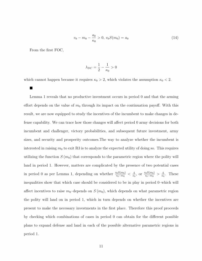
v0 −m0 −a0

κ0

> 0, v0S(m0) = a0 (14)

From the first FOC,

λDC =1

2− 1

κ0

> 0

which cannot happen because it requires κ0 > 2, which violates the assumption κ0 < 2.

�

Lemma 1 reveals that no productive investment occurs in period 0 and that the arming

effort depends on the value of m0 through its impact on the continuation payoff. With this

result, we are now equipped to study the incentives of the incumbent to make changes in de-

fense capability. We can trace how those changes will affect period 0 army decisions for both

incumbent and challenger, victory probabilities, and subsequent future investment, army

sizes, and security and prosperity outcomes.The way to analyze whether the incumbent is

interested in raising m0 to exit R3 is to analyze the expected utility of doing so. This requires

utilizing the function S (m0) that corresponds to the parametric region where the polity will

land in period 1. However, matters are complicated by the presence of two potential cases

in period 0 as per Lemma 1, depending on whether v0S(m0)v0−m0

< 4κ0

, or v0S(m0)v0−m0

> 4κ0

. These

inequalities show that which case should be considered to be in play in period 0–which will

affect incentives to raise m0–depends on S (m0), which depends on what parametric region

the polity will land on in period 1, which in turn depends on whether the incentives are

present to make the necessary investments in the first place. Therefore this proof proceeds

by checking which combinations of cases in period 0 can obtain for the different possible

plans to expand defense and land in each of the possible alternative parametric regions in

period 1.

11

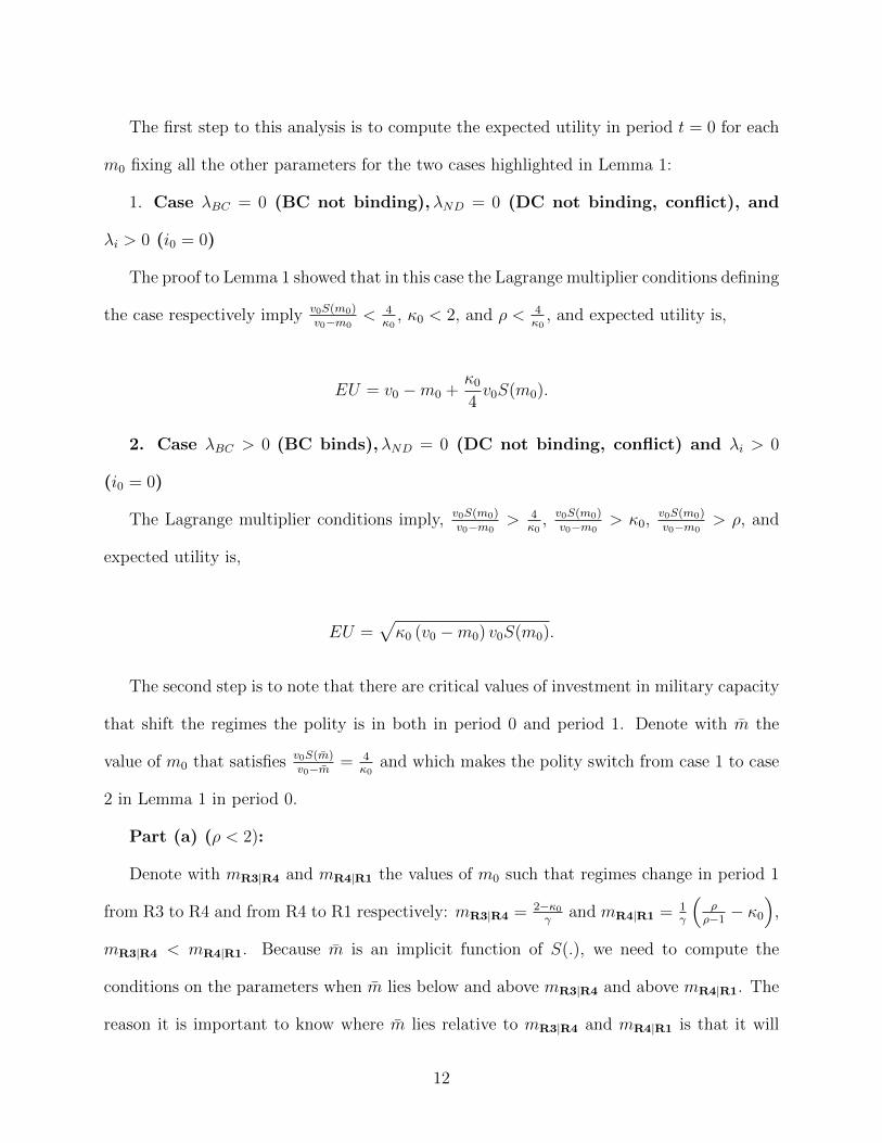
The first step to this analysis is to compute the expected utility in period t = 0 for each

m0 fixing all the other parameters for the two cases highlighted in Lemma 1:

1. Case λBC = 0 (BC not binding),λND = 0 (DC not binding, conflict), and

λi > 0 (i0 = 0)

The proof to Lemma 1 showed that in this case the Lagrange multiplier conditions defining

the case respectively imply v0S(m0)v0−m0

< 4κ0

, κ0 < 2, and ρ < 4κ0

, and expected utility is,

EU = v0 −m0 +κ0

4v0S(m0).

2. Case λBC > 0 (BC binds),λND = 0 (DC not binding, conflict) and λi > 0

(i0 = 0)

The Lagrange multiplier conditions imply, v0S(m0)v0−m0

> 4κ0

, v0S(m0)v0−m0

> κ0, v0S(m0)v0−m0

> ρ, and

expected utility is,

EU =√κ0 (v0 −m0) v0S(m0).

The second step is to note that there are critical values of investment in military capacity

that shift the regimes the polity is in both in period 0 and period 1. Denote with m the

value of m0 that satisfies v0S(m)v0−m = 4

κ0and which makes the polity switch from case 1 to case

2 in Lemma 1 in period 0.

Part (a) (ρ < 2):

Denote with mR3|R4 and mR4|R1 the values of m0 such that regimes change in period 1

from R3 to R4 and from R4 to R1 respectively: mR3|R4 = 2−κ0γ

and mR4|R1 = 1γ

(ρρ−1− κ0

),

mR3|R4 < mR4|R1. Because m is an implicit function of S(.), we need to compute the

conditions on the parameters when m lies below and above mR3|R4 and above mR4|R1. The

reason it is important to know where m lies relative to mR3|R4 and mR4|R1 is that it will

12

indicate which expected utility expression to use to evaluate choices of m0. If, for example,

m > mR4|R1 then we know the payoff from choosing an m0 that keeps the polity in R3, moves

it to R4 or an early part of R1 can be evaluated with a single expected utility expression,

namely that in case 1 from Lemma 1.

Before proving part (a) of Proposition 3 we need a technical result. The following lemma

establishes the conditions of the parameters that determine the value of m relative to mR3|R4

and mR4|R1.

Lemma 2 Under assumption 1,

i) If 0 < γv0 <8(2−κ0)8−3κ0

, then m < mR3|R4.

ii) If 8(2−κ0)8−3κ0

< γv0 <4κ0

( ρρ−1−κ0)

4κ0− (1+ρ)

ρ

, then mR3|R4 < m < mR4|R1

ii) If4κ0

( ρρ−1−κ0)

4κ0− (1+ρ)

ρ

< γv0, then mR4|R1 < m

Proof of lemma 2: To determine whether m lies within [0,mR3|R4], [mR3|R4,mR4|R1]

or [mR4|R1,∞] first notice that v0S(m0)v0−m0

is increasing in m0. Therefore, the conditions on the

parameters for each of these cases to hold are:

For m < mR3|R4 This is the case ifv0S(mR3|R4)

v0−mR3|R4> 4

κ0⇐⇒ v0γ <

8(2−κ0)8−3κ0

.

For mR3|R4 < m < mR4|R1 From above mR3|R4 < m ⇐⇒ 8(2−κ0)8−3κ0

< v0γ. Now we need

to find the condition for m < mR4|R1. This requiresv0S(mR4|R1)

v0−mR4|R1> 4

κ0, and this follows iff

v0γ <4κ0

( ρρ−1−κ0)

4κ0− (1+ρ)

ρ

. Therefore, this case occurs when

8(2− κ0)

8− 3κ0

< v0γ <

4κ0

(ρρ−1− κ0

)4κ0− (1+ρ)

ρ

For mR4|R1 < m It follows directly from before

13

4κ0

(ρρ−1− κ0

)4κ0− (1+ρ)

ρ

< v0γ

�

Due to this lemma 2, we know how to write expected utility depending on the value of

γv0, given all other parameters.

Part (a)1: We only need to find a cutoff in the space of possible values for γv0 such that

the incumbent prefers to stay in R3. We propose τL ≡ 8(2−κ0)8−3κ0

.

In this case, v0γ < 8(2−κ0)8−3κ0

is equivalent to a regime described by m < mR3|R4, which

means whe have to use two different EU expressions depending on whether m0 < m, or

m0 > m. Let us analyze the expected utility in each of these situations. A useful fact will be

that 8(2−κ0)8−3κ0

is strictly decreasing in κ0 so its maximum value is at κ0 = 1 (since κ0 > κc = 1).

In this case 8(2−1)8−3×1

= 85< 2.

Segment [0, m] Expected utility in period t = 0 is

EU = v0 − m0 + κ04v0S(m0) = v0 − m0 + κ0

4v0

(1 + κ0+γm0

4

)= v0(1 + κ0

4+(κ04

)2) +

m0

(κ0v0γ

16− 1)

Since m < mR3|R4 ⇐⇒ v0γ < 8(2−κ0)8−3κ0

then κ0v0γ16− 1 < 0. To see why, replace

v0γ = 8(2−κ0)8−3κ0

in κ0v0γ16

so κ0v0γ16

=κ0(

8(2−κ0)8−3κ0

)16

≤ κ085

16< 1. This implies EU is decreasing in m0

and the optimal choice is m0 = 0.

Segment [m,mR3|R4] Expected utility in period t = 0 is

EU =√κ0 (v0 −m0) v0S(m0) =

√κ0 (v0 −m0) v0

(1 + κ0+γm0

4

), and we now show this

to decrease in m0. Note,

dEUdm

= 12

[κ0 (v0 −m0) v0

(1 + κ0+γm0

4

)]− 12(−κ0v0

(1 + κ0+γm0

4

)+ γ

4κ0 (v0 −m0) v0

)and,

dEUdm

< 0 ⇐⇒ γ4κ0 (v0 −m0) v0 < κ0v0

(1 + κ0+γm0

4

), or, iff γv0 < 4 + κ0 + 2γm0.

14

If 4 + κ0 + 2γm0 is higher than 8(2−κ0)8−3κ0

, our condition to be in this scenario m <

mR3|R4

(⇐⇒ v0γ <

8(2−κ0)8−3κ0

)is a suficient condition for EU in this segment to be de-

creasing. So, it is sufficient to show that 4 + κ0 + 2γm0 > 8(2−κ0)8−3κ0

. Because the right

hand side is decreasing in κ0, it attains a maximum at κ0 = 1 and it is equal to 8/5

which is smaller than any feasible value of the expression in the left hand side, which

is at least 4. Therefore, in this segment utility is maximized at m0 = m, and equals

EU =√κ0 (v0 −m0) v0S(m0) =

√4(v0 − m)2 = 2 (v0 − m).

Segment [mR3|R4,mR4|R1] Since now m0 can only be larger than m, we know expected

utility is√κ0 (v0 −m0) v0S (m0). In R4, we have EU =

√κ0 (v0 −m0) v0

(2− 1

κ0+γm0

).

Computing the first derivative with respect to m0, we get,

dEU

dm0

=

(κ0 (v0 −m0) v0

(2− 1

κ0 + γm0

))− 12[−κ0v0

(2− 1

κ0 + γm0

)+κ0 (v0 −m0) v0γ

(κ0 + γm0)2

]

which is negative whenever 2 (κ0 + γm0)− 1 > (v0−m0)γκ0+γm0

, or, 2 (κ0 + γm0)2−κ0 > v0γ. Note

2(κ0 + γmR3|R4

)2 − κ0 = 8− κ0. Now note 8− κ0 >8(2−κ0)8−3κ0

≡ τL, since the LHS is at least

6 and the RHS is at most 85. Thus, dEU

dm0< 0 and utility would be maximized at mR3|R4 in

this segment.

Segment [mR4|R1,∞] Here, EU =√κ0 (v0 −m0) v0

(κ0+γm0)(1+ρ)κ0+γm0+ρ

and

dEUdm0

=(κ0 (v0 −m0) v0

(κ0+γm0)(1+ρ)κ0+γm0+ρ

)− 12

−κ0v0(κ0+γm0)(1+ρ)κ0+γm0+ρ

+κ0 (v0 −m0) v0γ(1+ρ)(κ0+γm0+ρ)−(κ0+γm0)(1+ρ)γ

(κ0+γm0+ρ)2

.

Note dEUdm0

< 0 whenever γv0 <(κ0+γm0+ρ)(κ0+γm0)

ρ+ γm0. The right hand side of this

expression is increasing in m0, so the minimum is attained at m0 = mR4|R1 and it equals

ρ(ρ−1)2

+ 2 ρ(ρ−1)

− κ0. The highest possible value of γv0, τL = 8(2−κ0)8−3κ0

is smaller than 85

which,

in turn, is always smaller than ρ(ρ−1)2

+2 ρ(ρ−1)

−κ0 given that ρ < 2. Therefore the maximum

15

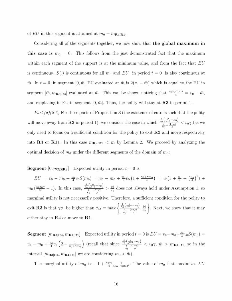
of EU in this segment is attained at m0 = mR4|R1.

Considering all of the segments together, we now show that the global maximum in

this case is m0 = 0. This follows from the just demonstrated fact that the maximum

within each segment of the support is at the minimum value, and from the fact that EU

is continuous. S(.) is continuous for all m0 and EU in period t = 0 is also continuous at

m. In t = 0, in segment [0, m] EU evaluated at m is 2(v0 − m) which is equal to the EU in

segment [m,mR3|R4] evaluated at m. This can be shown noticing that κ0v0S(m)4

= v0 − m,

and reeplacing in EU in segment [0, m]. Thus, the polity will stay at R3 in period 1.

Part (a)(2-3) For these parts of Proposition 3 (the existence of cutoffs such that the polity

will move away from R3 in period 1), we consider the case in which4κ0

( ρρ−1−κ0)

4κ0− (1+ρ)

ρ

< v0γ (as we

only need to focus on a sufficient condition for the polity to exit R3 and move respectively

into R4 or R1). In this case mR4|R1 < m by Lemma 2. We proceed by analyzing the

optimal decision of m0 under the different segments of the domain of m0:

Segment [0,mR3|R4] Expected utility in period t = 0 is

EU = v0 − m0 + κ04v0S(m0) = v0 − m0 + κ0

4v0

(1 + κ0+γm0

4

)= v0(1 + κ0

4+(κ04

)2) +

m0

(κ0v0γ

16− 1). In this case,

4κ0

( ρρ−1−κ0)

4κ0− (1+ρ)

ρ

> 16κ0

does not always hold under Assumption 1, so

marginal utility is not necessarily positive. Therefore, a sufficient condition for the polity to

exit R3 is that γv0 be higher than τM ≡ max

{4κ0

( ρρ−1−κ0)

4κ0− (1+ρ)

ρ

, 16κ0

}. Next, we show that it may

either stay in R4 or move to R1.

Segment [mR3|R4,mR4|R1] Expected utility in period t = 0 is EU = v0−m0+κ04v0S(m0) =

v0 − m0 + κ04v0

(2− 1

κ0+γm0

)(recall that since

4κ0

( ρρ−1−κ0)

4κ0− (1+ρ)

ρ

< v0γ, m > mR4|R1, so in the

interval [mR3|R4,mR4|R1] we are considering m0 < m).

The marginal utility of m0 is: −1 + κ0v04

γ(κ0+γm0)2

. The value of m0 that maximizes EU

16

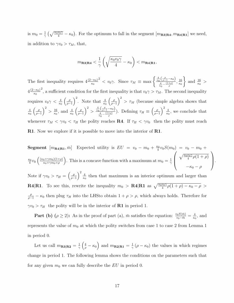
is m0 = 1γ

(√κ0v0γ

4− κ0

). For the optimum to fall in the segment [mR3|R4,mR4|R1] we need,

in addition to γv0 > τM , that,

mR3|R4 <1

γ

(√κ0v0γ

4− κ0

)< mR4|R1,

The first inequality requires 4 (2−κ0)κ0

2< v0γ. Since τM ≡ max

{4κ0

( ρρ−1−κ0)

4κ0− (1+ρ)

ρ

, 16κ0

}and 16

κ0>

4 (2−κ0)κ0

2, a sufficient condition for the first inequality is that v0γ > τM . The second inequality

requires v0γ < 4κ0

(ρρ−1

)2

. Note that 4κ0

(ρρ−1

)2

> τM (because simple algebra shows that

4κ0

(ρρ−1

)2

> 16κ0

, and 4κ0

(ρρ−1

)2

>4κ0

( ρρ−1−κ0)

4κ0− (1+ρ)

ρ

). Defining τH ≡(

ρρ−1

)24κ0

, we conclude that

whenever τM < γv0 < τH the polity reaches R4. If τH < γv0 then the polity must reach

R1. Now we explore if it is possible to move into the interior of R1.

Segment [mR4|R1, m] Expected utility is EU = v0 − m0 + κ04v0S(m0) = v0 − m0 +

κ04v0

((κ0+γm0)(1+ρ)κ0+γm0+ρ

). This is a concave function with a maximum atm0 = 1

γ

√κ0v0γ

4ρ(1 + ρ)

−κ0 − ρ

.

Note if γv0 > τH =(

ρρ−1

)24κ0

then that maximum is an interior optimum and larger than

R4|R1. To see this, rewrite the inequality m0 > R4|R1 as√

κ0v0γ4ρ(1 + ρ)− κ0 − ρ >

ρρ−1− κ0 then plug τH into the LHSto obtain 1 + ρ > ρ, which always holds. Therefore for

γv0 > τH the polity will be in the interior of R1 in period 1.

Part (b) (ρ ≥ 2): As in the proof of part (a), m satisfies the equation: v0S(m)v0−m = 4

κ0, and

represents the value of m0 at which the polity switches from case 1 to case 2 from Lemma 1

in period 0.

Let us call mR3|R2 = 1γ

(4ρ− κ0

)and mR2|R1 = 1

γ(ρ− κ0) the values in which regimes

change in period 1. The following lemma shows the conditions on the parameters such that

for any given m0 we can fully describe the EU in period 0.

17

Lemma 3 Under assumption 1,

i) If 0 < γv0 <16−4κ0ρ

4ρ−(1+ρ)κ0then m < mR3|R2

ii) If 16−4κ0ρ4ρ−(1+ρ)κ0

< γv0 <8(ρ−κ0)

8−(1+ρ)κ0then mR3|R2 < m < mR2|R1

ii) If 8(ρ−κ0)8−(1+ρ)κ0

< γv0 then mR2|R1 < m

Proof of lemma 3: It follows from replacing the definitions of m,mR3|R2,mR2|R1 and

following steps analogous to Lemma 2, as follows. To determine whether m lies within

[0,mR3|R2], [mR3|R2,mR2|R1] or [mR2|R1,∞] recall that v0S(m0)v0−m0

is increasing in m0. There-

fore, the conditions on the parameters for each of these cases to hold are:

For m < mR3|R2 This is the case whenv0S(mR3|R2)

v0−mR3|R2> 4

κ0⇐⇒ v0γ <

16−4κ0ρ4ρ−(1+ρ)κ0

.

For mR3|R2 < m < mR2|R1 From above mR3|R2 < m ⇐⇒ 16−4κ0ρ4ρ−(1+ρ)κ0

< v0γ. Now we

need to find the condition for m < mR2|R1. This requiresv0S(mR2|R1)

v0−mR2|R1> 4

κ0, or equivalently

v0γ <8(ρ−κ0)

8−(1+ρ)κ0. Therefore, this case occurs when

16− 4κ0ρ

4ρ− (1 + ρ)κ0

< v0γ <8(ρ− κ0)

8− (1 + ρ)κ0

(15)

For mR2|R1 < m It follows directly from before

8(ρ− κ0)

8− (1 + ρ)κ0

< v0γ.

�

Due to this lemma 3, we know how to write expected utility depending on the value of

γv0, given all other parameters.

Part (b)1 We need to find a cutoff such that the polity stays in R3. We propose σL ≡

16−4κ0ρ4ρ−(1+ρ)κ0

. In this case, v0γ < σL is equivalent to a regime in which m < mR3|R2 which means

18

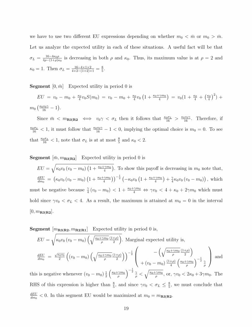
we have to use two different EU expressions depending on whether m0 < m or m0 > m.

Let us analyze the expected utility in each of these situations. A useful fact will be that

σL = 16−4κ0ρ4ρ−(1+ρ)κ0

is decreasing in both ρ and κ0. Thus, its maximum value is at ρ = 2 and

κ0 = 1. Then σL = 16−4×1×24×2−(1+2)×1

= 85.

Segment [0, m] Expected utility in period 0 is

EU = v0 − m0 + κ04v0S(m0) = v0 − m0 + κ0

4v0

(1 + κ0+γm0

4

)= v0(1 + κ0

4+(κ04

)2) +

m0

(κ0v0γ

16− 1).

Since m < mR3|R2 ⇐⇒ v0γ < σL then it follows that κ0σL16

> κ0v0γ16

. Therefore, if

κ0σL16

< 1, it must follow that κ0v0γ16− 1 < 0, implying the optimal choice is m0 = 0. To see

that κ0σL16

< 1, note that σL is at at most 85

and κ0 < 2.

Segment [m,mR3|R2] Expected utility in period 0 is

EU =√κ0v0 (v0 −m0)

(1 + κ0+γm0

4

). To show this payoff is decreasing in m0 note that,

dEUdm0

=(κ0v0 (v0 −m0)

(1 + κ0+γm0

4

))− 12(−κ0v0

(1 + κ0+γm0

4

)+ γ

4κ0v0 (v0 −m0)

), which

must be negative because γ4

(v0 −m0) < 1 + κ0+γm0

4⇔ γv0 < 4 + κ0 + 2γm0 which must

hold since γv0 < σL < 4. As a result, the maximum is attained at m0 = 0 in the interval

[0,mR3|R2].

Segment [mR3|R2,mR2|R1] Expected utility in period 0 is,

EU =

√κ0v0 (v0 −m0)

(√κ0+γm0

ρ(1+ρ)

2

). Marginal expected utility is,

dEUdm0

=√κ0v02

((v0 −m0)

(√κ0+γm0

ρ(1+ρ)

2

))− 12

−(√

κ0+γm0

ρ(1+ρ)

2

)+ (v0 −m0) (1+ρ)

4

(κ0+γm0

ρ

)− 12 γρ

and

this is negative whenever (v0 −m0) 12

(κ0+γm0

ρ

)− 12 γρ<√

κ0+γm0

ρ, or, γv0 < 2κ0 + 3γm0. The

RHS of this expression is higher than 85, and since γv0 < σL ≤ 8

5, we must conclude that

dEUdm0

< 0. In this segment EU would be maximized at m0 = mR3|R2.

19

Segment [mR2|R1,∞] Expected utility in period 0 is,

EU =√κ0v0 (v0 −m0) (κ0+γm0)(1+ρ)

κ0+γm0+ρ. Marginal expected utility is,

dEUdm0

=√κ0v02

((v0 −m0) (κ0+γm0)(1+ρ)

κ0+γm0+ρ

)− 12

− (κ0+γm0)(1+ρ)κ0+γm0+ρ

+ (v0 −m0) (1 + ρ) ρ

(κ0+γm0+ρ)2

. This is

negative whenever (v0 −m0) ρκ0+γm0+ρ

< (κ0 + γm0), or whenever,

v0γ <1

ρ(κ0 + γm0)2 + (κ0 + γm0) + γm0.

The right hand side of this expression is increasing in m0, so the minimum of this expression

is attained at m0 = mR2|R1 and it equals 3ρ−κ0. Since γv0 <85< 3ρ−κ0 the result follows.

In sum, the global maximum when m < mR3|R2

(⇐⇒ v0γ <

16−4κ0ρ4ρ−(1+ρ)κ0

= σL

)is

m0 = 0. This follows from the just demonstrated fact that the maximum within each

segment of the support is at the minimum point, and from the fact that EU is continuous.

S(.) is continuous for all m0 and hence EU in period 0 is also continuous at m. In period 0 in

segment [0, m], EU evaluated at m is 2(v0−m) which is equal to EU in segment [m,mR3|R2]

evaluated at m. This can be shown noticing that κ0v0S(m)4

= v0−m, and substituting into the

expression for EU in segment [0, m]. Thus, the polity will stay at R3 in period 1 whenever

γv0 < σL. Next, we show that there exist σH = 16/κ0 > σM2, such that the polity moves to

R1.

Part (b)(2) To prove the existence of values for γv0 high enough that the polity will move

away from R3 into R1, consider the case in which 16κ0< γv0. Note that 8(ρ−κ0)

8−(1+ρ)κ0< 16

κ0, so

mR2|R1 < m. We proceed by analyzing the optimal m0 in each segment in what follows.

Segment [0,mR3|R2] Expected utility in period t = 0 is,

EU = v0 − m0 + κ04v0S(m0) = v0 − m0 + κ0

4v0

(1 + κ0+γm0

4

)= v0(1 + κ0

4+(κ04

)2) +

m0

(κ0v0γ

16− 1). Marginal utility is positive iff γv0 > 16

κ0, so the polity moves to R2, or

20

advances to R1.

Segment [mR3|R2,mR2|R1] The (concave) expected utility is, EU = v0−m0+κ0v0(1+ρ)8

√κ0+γm0

ρ.

The marginal utility of m0 is: −1+ κ0v0(1+ρ)8

12

√ρ

κ0+γm0

γρ. This marginal utility may be either

negative, zero or positive in [mR3|R2,mR2|R1]. Given concavity, it is negative iff the value at

which the marginal utility is zero, m0 =

(κ0v0γ

161+ρ√ρ

)2−κ0

γ, is smaller than mR3|R2:

m0 =

(κ0v0γ

161+ρ√ρ

)2

− κ0

γ< mR3|R2 =

(4ρ− κ0)

γ

⇐⇒ v0γ <(

16κ0

)2

1+ρ. In this case, the maximum EU in this segment is at m0 = mR3|R2.

The solution is interior in R2 if m0 =

(κ0v0γ

16(1+ρ)√

ρ

)2−κ0

γis in between mR3|R2 and mR2|R1:

(4ρ− κ0)

γ= mR3|R2 <

(κ0v0γ

16(1+ρ)√

ρ

)2

− κ0

γ< mR2|R1 =

(ρ− κ0)

γ

⇐⇒ 16κ0

21+ρ

< v0γ <16κ0

ρ1+ρ

. But since 16κ0

ρ1+ρ

< 16κ0

, then v0γ >16κ0

ρ1+ρ

and the incumbent

moves to R1. The following analysis shows the incumbent moves to the interior of R1 in

this case.

Segment [mR2|R1, m] Expected utility is EU = v0 − m0 + κ04v0S(m0) = v0 − m0 +

κ0v04

((κ0+γm0)(1+ρ)κ0+γm0+ρ

), and marginal utility is dEU

dm0= κ0v0

4(κ0+γm0+ρ)γ(1+ρ)−(κ0+γm0)γ(1+ρ)

(κ0+γm0+ρ)2=

κ0v04

γρ(1+ρ)

(κ0+γm0+ρ)2− 1, so the interior optimum is

m0 = 1γ

(√κ0v0γ

4ρ(1 + ρ)− κ0 − ρ

). It is straightforward (using arguments analogous

to the case in segment [mR3|R2,mR2|R1]) to show that if 16κ0

ρ(1+ρ)

< γv0 then we also have

m0 = 1γ

(√κ0v0γ

4ρ(1 + ρ)− κ0 − ρ

)> mR2|R1. This implies that for γv0 > 16

κ0= σH the

polity must move to the interior of R1 in period 1.

21

In sum, whenever σH < γv0 the polity moves to R1. In what follows, we show that there

exist

σM1 = max

16− 4κ0ρ

4ρ− (1 + ρ)κ0

,

4κ0−√(

4κ0

)2

− 3× (1+ρ)2

ρ

(κ04

)2× (1+ρ)2

ρ

(κ016× 3

4

)

σM2 = min

8(ρ− κ0)

8− (1 + ρ)κ0

,

4κ0

+

√(4κ0

)2

− 3× (1+ρ)2

ρ

(κ04

)2× (1+ρ)2

ρ

(κ016× 3

4

) , 3ρ− κ0

,

with σL < σM1 < σH and σL < σM2 < σH , such that the polity moves to R2 whenever

σM1 < γv0 < σM2.

Part (b)(3) To prove the existence of values of γv0 such that the polity will move into

R2, consider the case in which (15) holds, so mR3|R2 < m < mR2|R1. We characterize the

set of parameters (κ0, ρ) such that the optimal point lies in R2.

Segment [0,mR3|R2] Expected utility in period t = 0 is, EU = v0 −m0 + κ04v0S(m0) =

v0 − m0 + κ04v0

(1 + κ0+γm0

4

)= v0(1 + κ0

4+(κ04

)2) + m0

(κ0v0γ

16− 1). Marginal utility is

positive iff γv0 >16κ0

and negative iff γv0 <16κ0

. Algebra shows that under Assumption 1

16−4κ0ρ4ρ−(1+ρ)κ0

< 8(ρ−κ0)8−(1+ρ)κ0

< 16κ0

. Thus, m0 = 0 is optimal in [0,mR3|R2] and the polity will stay

in R3. EU evaluated at m0 = 0 is v0(1 + κ04

+(κ04

)2), and we later show that this value is

lower than EU at the optimum in R2 whenever σM1 < γv0 < σM2.

Segment [mR3|R2, m] There are two possibilities for an optimum in R2. It could lie in

[mR3|R2, m] or in [m,mR2|R1]. We only need to show the result for one of the two cases so

we focus on the first. The (concave) expected utility is,

EU = v0−m0+κ0v0(1+ρ)8

√κ0+γm0

ρ. The marginal utility ofm0 is: −1+κ0v0(1+ρ)

812

√ρ

κ0+γm0

γρ.

Hence, the optimum point is given by mIntR2 =

(κ0v0γ

161+ρ√ρ

)2−κ0

γ. This point is less than m if

22

and only if v0S(mIntR2)v0−mIntR2

< 4κ0

, which is equivalent to,

4κ0−√(

4κ0

)2

− 3× (1+ρ)2

ρ

(κ04

)2× (1+ρ)2

ρ

(κ016× 3

4

) < γv0 <

4κ0

+

√(4κ0

)2

− 3× (1+ρ)2

ρ

(κ04

)2× (1+ρ)2

ρ

(κ016× 3

4

) . (16)

Then EU (mIntR2) is 1γ

(γv0

(1 + v0γ

(κ016

(1+ρ)√ρ

)2)

+ κ0

). Hence, the optimal value lies in

[mR3|R2, m] if EU (mIntR2) > EU (m0 = 0). This inequality implies (after some algebra)

that(κ04

(1 + κ0

4

)− κ0

γ

)(16κ0

√ρ

(1+ρ)

)2

< v0γ. Note the LHS of this expression is negative as

long as γ < 16/(4 + κ0), the technical assumption introduced in the text.

Our strategy for this part of the proof is to find the combinations of (κ0, ρ) for which

EU (mIntR2) > EU (m0 = 0). This is a sufficient condition for the optimal point to lie in R2

as long as EU is decreasing in m0 over R1.

Segment [mR2|R1,∞] Expected utility is

EU =√κ0v0 (v0 −m0)S(m0) =

√κ0v0 (v0 −m0) (κ0+γm0)(1+ρ)

κ0+γm0+ρ. Marginal utility is,

dEUdm0

=√κ0v0

12

[− (v0 −m0)−

12

√(κ0+γm0)(1+ρ)κ0+γm0+ρ

+√

(v0 −m0)(

(κ0+γm0)(1+ρ)κ0+γm0+ρ

)− 12 γρ(1+ρ)

(κ0+γm0+ρ)2

].

Note dEUdm0

< 0 iff −(κ0 +γm0)(κ0 +γm0 +ρ) +γρ (v0 −m0) < 0. The LHS of this expression

is decreasing in m0 so if evaluated at mR2|R1 = ρ−κ0γ

such LHS is negative, then EU is

decreasing in m0 within R1. Evaluating at mR2|R1 = ρ−κ0γ

yields,

γv0 < 3ρ− κ0. (17)

Combining (15), (16), and (17), we define σM1 = max

16−4κ0ρ4ρ−(1+ρ)κ0

,4κ0−√(

4κ0

)2−3× (1+ρ)2

ρ (κ04 )

2× (1+ρ)2

ρ (κ016×34)

and σM2 = min

8(ρ−κ0)8−(1+ρ)κ0

,4κ0

+

√(4κ0

)2−3× (1+ρ)2

ρ (κ04 )

2× (1+ρ)2

ρ (κ016×34)

, 3ρ− κ0

. As a result, if σM1 < γv0 <

23

σM2 then the polity moves to R2. Note the set over the real line bounded by σM1 and σM2

is non-empty for a measurable set of (κ0, ρ). For example, fix ρ = 4 κ0 = 1. In this case, the

conditions (15), (16), and (17) become respectively 0 < γv0 < 8,516−√

( 516)

2−4( 5

16×2)2

2( 532)

2 < 0 <

γv0 <325

and γv0 < 11.Hence, σM1 = 0 and σM2 = 32/5 and for 0 < γv0 < 32/5 the polity

moves to R2. As these inequalities are strict, pairs (ρ, κ0) in a neighborhood of (4, 1) also

yield a transition to R2 for a measurable set of γv0.

In sum, there exist σL, σM1, σM2 and σH defined above, σL < σM1 < σH and σL <

σM2 < σH , (simple algebra shows that σM1 < σH and σM2 < σH) such that if γv0 < σL the

polity stays in R3; if σM1 < γv0 < σM2 the polity moves from R3 to R2; and if γv0 > σH

the polity moves from R3 to R1.�

24