The Ornstein-Uhlenbeck Dirichlet Process and other time

The Ornstein-Uhlenbeck Dirichlet Process and other

time-varying processes for Bayesian nonparametric

inference

J.E. Griffin∗

Department of Statistics, University of Warwick, Coventry, CV4 7AL, U.K.

Abstract

This paper introduces a new class of time-varying, meaure-valued stochastic processes

for Bayesian nonparametric inference. The class of priors generalizes the normalized ran-

dom measure (Kingman 1975) construction for static problems. The unnormalized measure

on any measureable set follows an Ornstein-Uhlenbeck process as described by Barndorff-

Nielsen and Shephard (2001). Some properties of the normalized measure are investigated.

A particle filter and MCMC schemes are described for inference. The methods are applied

to an example in the modelling of financial data.

1 Introduction

Bayesian nonparametric models based on Dirichlet process mixtures have been popular for

clustering and density estimation problems. Muller and Quintana (2004) give a comprehen-

sive review of these ideas. The model assumes that the datay1, . . . , yn are an i.i.d. sample

from a distribution with densityf which can be expressed asf(y) =∫

k(y|θ) dG(θ) where

k(y|θ) is a continuous density function, which will be referred to as a kernel. A prior,Π,

∗Corresponding author: Jim Griffin, Department of Statistics, University of Warwick, Coventry, CV4 7AL, U.K.

Tel.: +44-1227-82 3865; Fax: +44-24-7652 4532; Email: [email protected].

1

CRiSM Paper No. 07-3, www.warwick.ac.uk/go/crism

will be placed onG that allows a wide support forf . The model can also be represented

hierarchically

yi ∼ k(yi|θi)

θi ∼ F

F ∼ Π.

A popular choice forΠ is the Dirichlet process (Ferguson, 1973). There has recently been

some criticism of the Dirichlet process specification and alternatives have been proposed in-

cluding: Normalised Inverse Gaussian (NIG) processes (Lijoi et al 2005), Normalised Gen-

eralized Gamma Process (Lijoiet al 2006), and Stick-Breaking Priors (Ishwaran and James

2001, 2003).

Suppose that we know thei-th observation,yi, is made at timeti. The extension of this

nonparametric mixture model to these data has been an area ofrecent interest. A natural

extension to the nonparametric model assumes thatf(y|t), the distribution ofy at timet, can

be expressed asf(y|t) =∫

k(y|θ) dGt(θ). The prior specification is completed by defining

a prior distribution forGt over a suitable range of values oft. If the observations arrive in

discrete time then a prior can be defined by the recursion

Gt+1 = wtGt + (1 − wt)εt (1)

whereεt is a realisation of a random discrete distribution andwt is a random variable in

the interval(0, 1). Pennell and Dunson (2006) consider a time-invariantwt and a Dirichlet

process with time-invariant parameters forεt. Griffin and Steel (2006a) consider constructing

a process wherew1, w2, w3, . . . are i.i.d. Beta(1,M ) random variables andεt is a distribution

concentrated on a single point drawn from some distributionH. The dependence structure

can be modelled by subordinating this process to a Poisson process with intensityλ, . This

construction ensures that ifGt follows a Dirichlet process then so willGt+j . An alternative

approach is considered by Zhuet al (2005) who specify the predictive distribution ofyn+1,

observed at timetn+1, which is proportional to

n∑

i=1

exp{−λ(tn+1 − ti)}δyi+MH

whereδx is the Dirac measure that places mass 1 onx andλ andM are positive parameters,

that will control the marginal process and the dependence between distributions at different

times. The form generalizes the famous Polya urn scheme representation of the Dirichlet

process (Blackwell and MacQueen 1974).

This paper develops an alternative approach which guarantees stationarity of the finite

distribution of the measure-valued process using the Ornstein-Uhlenbeck (OU) processes

2


with non-Gaussian marginal distributions developed by Barndorff-Nielsen and Shephard (2001),

which will henceforth be referred to as BNS, for financial modelling. This implies that the

marginal process at any time is known, which gives some intuition about the behaviour of

the process and allows separate elicitation of parameters for the marginal process and the de-

pendence structure. The construction mimics the approach of Zhu et al (2005) by defining an

exponential decay for a process proportional toGt. The process is defined in continuous time

but in discrete time it will have a structure like (1) whereεt usually has an infinite number of

atoms. Markov chain Monte Carlo and particle filtering methods are proposed for posteriors

simulation which involve a truncation of the random process. Dirichlet process marginals are

an interesting exception and arise from a process with an increment that has a finite number

of atoms. Consequently, MCMC and particle filtering methodsfor this class can be defined

without truncation. The paper is organized in the followingway: Section 2 reviews the

Normalized Random Measures (NRM) class of priors and the construction of OU processes

with specified marginal distributions, Section 3 uses theseideas to construct measure valued

processes whose marginal process follow specific NRMs, Section 4 describes both Markov

chain Monte Carlo and particle filtering methods for inference, Section 5 applies these meth-

ods to financial time series, and Section 6 dicusses the future development of these types of

processes.

2 Background

2.1 Normalized random measures

Normalized random measures (NRMs) have played an importantrole in Bayesian nonpara-

metrics since the Dirichlet process was introduced as a normalized Gamma process by Fer-

guson (1973). The idea was generalized by Kingman (1975) whotakes a Poisson process

on (0,∞) say J1 > J2 > J3 > . . . such that∑∞

i=1 Ji is finite and defines probabili-

tiespi = JiP∞i=1 Ji

. A random probability measure can be defined byG =∑∞

i=1JiP∞i=1 Ji

δθi

whereθ1, θ2, θ3, . . . are independently drawn from some distributionH. This guarantees that

E[G(B)] = H(B). It will useful to consider the unnormalized measureG? =∑∞

i=1 Jiδθi.

If the support ofH is S thenG = G?

G?(S) . The class was extended by Regazziniet al (2003)

to increasing additive processes in one-dimension and by Jameset al (2005) to multivariate

processes. The construction of Jameset al (2005) re-expresses Kingman (1975) approach by

defining a Poisson process with intensityν(J, θ) on (0,∞)×S whereS is the support ofH.

Jameset al (2005) refer to an NRM ashomogeneousif the intensity function has the form,

ν(J, θ) = W+(J)h(θ) whereh is differentiable. This paper will concentrate on this homo-

geneous case and define this process to be NRM(W+,H). In this paper, the construction

3


will be extended to a third dimension, time, using a representation of the BNS OU process.

2.2 The Gamma OU process

This section describes the development of OU processes withgiven non-Gaussian marginal

distribution and draws heavily on the material in BNS. Suppose thatz(t) is a Levy process

(e.g.Sato, 1999 or Bertoin, 1996) which has dynamics governed by the Stochastic Differen-

tial Equation

dZ(t) = −λZ(t) + dφ(λt)

whereφ(t) is called the background driving Levy process (BDLP). BNS show that the Levy

densityu of Z(t) is linked to Levy densityw of φ(t) by the following relationship

w(x) = −u(x) − xu′(x)

which implies that the tail integral functionW+(x) has the form

W+(x) =

∫ ∞

xw(y) dy = xu(x).

This will be an important function for the definition of OU-type processes with specified

NRM marginal processes.

Example 1: Gamma

Suppose thatZ(t) ∼ Ga(ν, α) with density αν

Γ(ν)xν−1 exp{−αx} then

W+(x) = ν exp{−αx}.

Example 2: Inverse Gaussian

Suppose thatZ(t) follows an Inverse Gaussian distribution which has density

δ√2π

exp{δγ}x−3/2 exp

{

−1

2(δ2x−1 + γ2x)

}

then

W+(x) =δ√2πx−1/2 exp

{

−1

2γ2x

}

.

Ferguson and Klass (1972) describe how a Levy process can beexpressed as a transfor-

mation of a Poisson process. First we write the process as

Z(t) = exp{−λt}Z(0) +

∫ t

0exp{−λ(t− s)}du(λs). (2)

4


The stochastic integral can be expressed using the Fergusonand Klass (1972) method as

∫ t

0f(s) du(λs)

d=

∞∑

i=1

W−1( ai

λt

)

f(λτi)

whereai andτi are two independent sequences of random variables with theτi independent

copies of a uniform random variableτ on [0, t], a1 < a2 < · · · < ai < . . . as the arrival

times of a Poisson process with intensity 1 andW−1 is the inverse of the tail mass function

W+(x). This representation suggest an alternative interpretation in terms of a jump sizes

Ji = W−1(

ai

λt

)

and an arrival timesτi. Let (J, τ) be a Poisson process on(0,∞) × [0, t]

with intensityλW+(J) then

∫ t

0f(s) du(λs)

d=

∞∑

i=1

Jif(τi).

This can clearly be extended to

∫ t

−∞f(s) du(λs)

d=

∞∑

i=1

I(τi < t)Jif(τi)

where(J, τ) be a Poisson process on(0,∞) × (−∞,∞) with intensityλW+(J).

Example 1: Gamma (continued)

Usually the inverse tail mass functionW−1 will not be available analytically. However, if

the process has a marginal Gamma distribution with parameters ν andα then

W−1(x) = max

{

0,− 1

αlog(x

ν

)

}

∫ t

0exp{−λs} du(λs) d

=

∞∑

i=1

max

{

0,− 1

αlog( ai

λνt

)

}

exp{−λτi}

We are interested in Gamma distribution with shape 1 so we canre-write the expression in

the following way

∫ t

0exp{−λs} du(λs) d

=∞∑

i=1

[− log ai] exp{−λτi}

whereai is a Poisson process with intensityλν.

5


3 The OUNRM processes

The Ferguson and Klass (1972) representation of the BNS OU L´evy process and Jameset

al (2005)’s representation of the NRM process are both expressed through functions of Pois-

son processes. The OUNRM process combines these two ideas togive a Poisson process-

based definition. For any NRM process, the distribution of the unnormalized measureG? on

any measureable setB has a known form. If we define a time-varying unnormalized measure

G?t , then its marginal distribution on a measureable setB can be fixed over time using the

BNS OU process. This leads to the following definition.

Definition 1 Let(τ, J, θ) be a Poisson process onR×R+×S which has intensityλW+(J)h

and define

Gt =∞∑

i=1

I(τi ≤ t) exp{−λ(t− τi)}Ji∑∞

i=1 I(τi ≤ t) exp{−λ(t− τi)}Jiδθi

then{Gt}t∈R follows anOUNRM process, which will be writtenOUNRM(W+(x),H, λ)

Theorem 1 If {Gt}t∈R follows anOUNRM(W+(x),H, λ) process thenGt follows anNRM(W+(x),H)

for all t.

The process can be defined in the form of equation (1) as a mixture ofGt and an innova-

tion εt where

wt =exp{−λ}G?

t−1(S)

exp{−λ}G?t−1(S) +

∑

I(t− 1 < τi < t) exp{−λ(τi − t+ 1)}Ji(3)

whereG?(t− 1) =∑∞

i=1 I(τi ≤ t− 1) exp{−λ(t − 1 − τi)Ji} which by construction will

have the distribution of the unnormalized measure onS and

εt =

∑

I(t− 1 < τi < t) exp{−λ(τi − t+ 1)}δθiJi

∑

I(t− 1 < τi < t) exp{−λ(τi − t+ 1)}Ji. (4)

The weightwt will, in general, be correlated withGt and εt+1. An important exception

is the process with a marginal Dirichlet process, which willbe developed in the follow-

ing subsection. The recursion leads to the following Markovstructure forGt+1|Gt =

E [wt|Gt]Gt + E [(1 − wt)εt|Gt]. The process is mean-reverting for all measureable sets.

This recursion for the unknown probability distribution naturally extends to expectations of

functionals of the unknown distribution. Let Et[a(X)] =∫

a(X) dGt(X). If this expectation

exists then

Et+1[a(X)]|Et[a(X)]d= E[wt]Et[a(X)] + (1 − E[wt])µ

whereµ is the expectation ofa(X) with respect to the centring distributionH.

A useful summary of the dependence is given by the autocorrelation function of the

measure on a setB, which was suggested by Mallick and Walker (1997). In general the

6


autocorrelation can be calculated directly from equation (3) and (4) combined with the sta-

tionarity of the process. The autocorrelation function will decay like an exponential function

asymptotically but at a slower rate for smallt. The effect will be observed in plots for the

Dirichlet process marginal case.

Result 1

The autocorrelation decays likeexp{−λt} if E[

1G?

t (S)

]

exists. Otherwise the autocorrelation

will decay at a slower rate.

3.1 The OUDP process

The OUDP is an important subclass of these processes for two reasons: firstly, the Dirichlet

process has been the most extensively applied example of an NRM and secondlyG?t (S) is

independent ofGt(B) for all B, which leads to some simplified expressions for summaries

of the process. The Dirichlet process (Ferguson, 1973) is defined by normalising a Gamma

process with mass parameterMH and will be written DP(M,H). The parameterM is

usually considered a precision parameter since ifG follows a DP(M,H) then Var(G(B)) =H(B)(1−H(B))

M+1 .

Definition 2 Let(τ, J, θ) be a Poisson process onR×R+×S which has intensityMλ exp{−J}h

and define

Gt =

∞∑

i=1



then{Gt}t∈R follows anOUDP processwhich we will writeOUDP(M,H,λ)

Corollary 1 If {Gt}t∈R follows anOUDP(M,H,λ) thenGt follows a Dirichlet process

with mass parameterMH for all t.

It follows from the independence ofGt(B) andG?t (S) that

Cov(Gt, Gt+k) = E

t+k−1∏

j=t

wj

Var(Gt).

The stationarity ofGt implies that if the marginal process follows a Dirichlet process then

the autocorrelation is

Corr(Gt, Gt+k) = E

[

exp{−λk}G?t (S)

exp{−λk}G?t (S) +

∑

I(τi < k) exp{−λτi}Ji

]

.

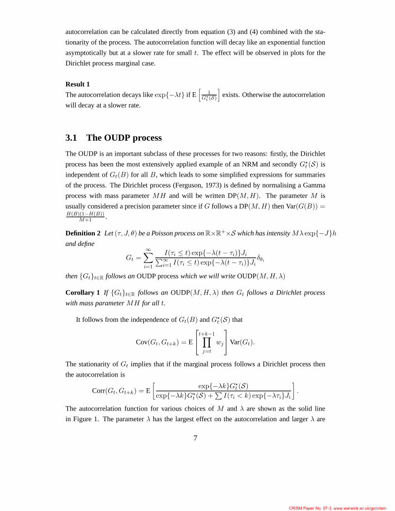
The autocorrelation function for various choices ofM andλ are shown as the solid line

in Figure 1. The parameterλ has the largest effect on the autocorrelation and largerλ are

7


λ = 0.125 λ = 0.25 λ = 0.5 λ = 1 λ = 2

M = 1

0 1 2 3 4 5 6 7 8 9 100.4

0.5

0.6

0.7

0.8

0.9

1

0 1 2 3 4 5 6 7 8 9 100.1

0.2

0.3

0.4

0.5

0.6

0.7

0.8

0.9

1

0 1 2 3 4 5 6 7 8 9 100

0.1

0.2

0.3

0.4

0.5

0.6

0.7

0.8

0.9

1

0 1 2 3 4 5 6 7 8 9 100

0.1

0.2

0.3

0.4

0.5

0.6

0.7

0.8

0.9

1

0 1 2 3 4 5 6 7 8 9 100

0.1

0.2

0.3

0.4

0.5

0.6

0.7

0.8

0.9

1

M = 4

0 1 2 3 4 5 6 7 8 9 100.3

0.4

0.5

0.6

0.7

0.8

0.9

1

0 1 2 3 4 5 6 7 8 9 100.1

0.2

0.3

0.4

0.5

0.6

0.7

0.8

0.9

1

0 1 2 3 4 5 6 7 8 9 100

0.1

0.2

0.3

0.4

0.5

0.6

0.7

0.8

0.9

1

0 1 2 3 4 5 6 7 8 9 100

0.1

0.2

0.3

0.4

0.5

0.6

0.7

0.8

0.9

1

0 1 2 3 4 5 6 7 8 9 100

0.1

0.2

0.3

0.4

0.5

0.6

0.7

0.8

0.9

1

M = 16

0 1 2 3 4 5 6 7 8 9 100.2

0.3

0.4

0.5

0.6

0.7

0.8

0.9

1

0 1 2 3 4 5 6 7 8 9 100

0.1

0.2

0.3

0.4

0.5

0.6

0.7

0.8

0.9

1

0 1 2 3 4 5 6 7 8 9 100

0.1

0.2

0.3

0.4

0.5

0.6

0.7

0.8

0.9

1

0 1 2 3 4 5 6 7 8 9 100

0.1

0.2

0.3

0.4

0.5

0.6

0.7

0.8

0.9

1

0 1 2 3 4 5 6 7 8 9 100

0.1

0.2

0.3

0.4

0.5

0.6

0.7

0.8

0.9

1

Figure 1: The autocorrelation function of the OUDP for various values ofM andλ (solid line)

with the approximation of result 2 (dashed line)

associated with more quickly decaying autocorrelation functions. For a fixedλ, smaller

values ofM lead to a more slowly decaying autocorrelation function andin fact if M ≤ 1

then result 1 shows that the autocorrelation will decay at a sub-exponential rate. IfM > 1,

then Corr(Gt, Gt+k) → MM−1 exp{−λk} ask → ∞. It is useful in these case to have an

approximation of the autocorrelation function, which can be derived using the delta method,

Corr(Gt, Gt+k) ≈ exp{−λk}[

1 +σ2

µ2(1 − exp{−λk})

]

whereµ = E[G?(S)] andσ2 = V[G?(S)].

The actual autocorrelation and the approximate autocorrelation are shown in figure 1. If

σ2 is small relative toµ2, which happens in the Dirichlet process asM → ∞, the approx-

imate autocorrelation becomes increasingly like an exponential function (in other words it

inherits the dependence in the unnormalized random measure) and it has a much slower rate

of decay when the ratio is large, which is illustrated by the cases with smallM . A second as-

pect of the dependence is captured through the moments of theunknown distribution. In this

case we can show the moments themselves follow the same type of process as the measures

on a setB.

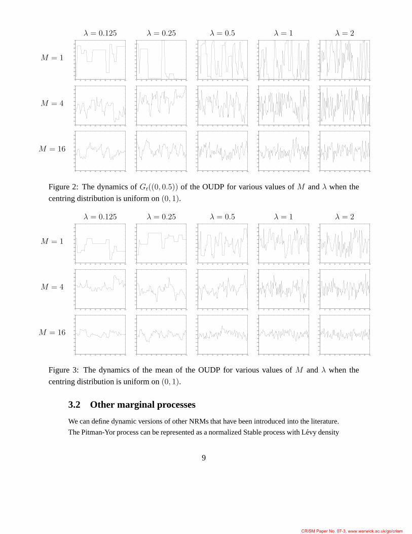
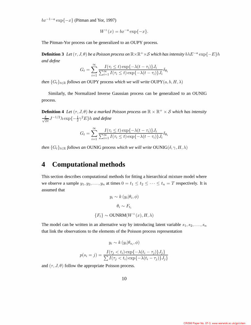
Figures 2 and 3 show the effect ofλ andM on the dependence structure and variability

of Gt((0, 0.5)) and the mean of distribution when the Dirichlet process is centred over a

uniform distribution. Large values ofM leads to smaller variability and large values ofλ

lead to quicker mean reversion of the process.

8


λ = 0.125 λ = 0.25 λ = 0.5 λ = 1 λ = 2

M = 1

0 10 20 30 40 50 60 70 80 90 1000

0.1

0.2

0.3

0.4

0.5

0.6

0.7

0.8

0.9

1

0 10 20 30 40 50 60 70 80 90 1000

0.1

0.2

0.3

0.4

0.5

0.6

0.7

0.8

0.9

1

0 10 20 30 40 50 60 70 80 90 1000

0.1

0.2

0.3

0.4

0.5

0.6

0.7

0.8

0.9

1

0 10 20 30 40 50 60 70 80 90 1000

0.1

0.2

0.3

0.4

0.5

0.6

0.7

0.8

0.9

1

0 10 20 30 40 50 60 70 80 90 1000

0.1

0.2

0.3

0.4

0.5

0.6

0.7

0.8

0.9

1

M = 4

0 10 20 30 40 50 60 70 80 90 1000

0.1

0.2

0.3

0.4

0.5

0.6

0.7

0.8

0.9

1

0 10 20 30 40 50 60 70 80 90 1000

0.1

0.2

0.3

0.4

0.5

0.6

0.7

0.8

0.9

1

0 10 20 30 40 50 60 70 80 90 1000

0.1

0.2

0.3

0.4

0.5

0.6

0.7

0.8

0.9

1

0 10 20 30 40 50 60 70 80 90 1000

0.1

0.2

0.3

0.4

0.5

0.6

0.7

0.8

0.9

1

0 10 20 30 40 50 60 70 80 90 1000

0.1

0.2

0.3

0.4

0.5

0.6

0.7

0.8

0.9

1

M = 16

0 10 20 30 40 50 60 70 80 90 1000

0.1

0.2

0.3

0.4

0.5

0.6

0.7

0.8

0.9

1

0 10 20 30 40 50 60 70 80 90 1000

0.1

0.2

0.3

0.4

0.5

0.6

0.7

0.8

0.9

1

0 10 20 30 40 50 60 70 80 90 1000

0.1

0.2

0.3

0.4

0.5

0.6

0.7

0.8

0.9

1

0 10 20 30 40 50 60 70 80 90 1000

0.1

0.2

0.3

0.4

0.5

0.6

0.7

0.8

0.9

1

0 10 20 30 40 50 60 70 80 90 1000

0.1

0.2

0.3

0.4

0.5

0.6

0.7

0.8

0.9

1

Figure 2: The dynamics ofGt((0, 0.5)) of the OUDP for various values ofM andλ when the

centring distribution is uniform on(0, 1).

λ = 0.125 λ = 0.25 λ = 0.5 λ = 1 λ = 2

M = 1

0 10 20 30 40 50 60 70 80 90 1000

0.1

0.2

0.3

0.4

0.5

0.6

0.7

0.8

0.9

1

0 10 20 30 40 50 60 70 80 90 1000

0.1

0.2

0.3

0.4

0.5

0.6

0.7

0.8

0.9

1

0 10 20 30 40 50 60 70 80 90 1000

0.1

0.2

0.3

0.4

0.5

0.6

0.7

0.8

0.9

1

0 10 20 30 40 50 60 70 80 90 1000

0.1

0.2

0.3

0.4

0.5

0.6

0.7

0.8

0.9

1

0 10 20 30 40 50 60 70 80 90 1000

0.1

0.2

0.3

0.4

0.5

0.6

0.7

0.8

0.9

1

M = 4

0 10 20 30 40 50 60 70 80 90 1000

0.1

0.2

0.3

0.4

0.5

0.6

0.7

0.8

0.9

1

0 10 20 30 40 50 60 70 80 90 1000

0.1

0.2

0.3

0.4

0.5

0.6

0.7

0.8

0.9

1

0 10 20 30 40 50 60 70 80 90 1000

0.1

0.2

0.3

0.4

0.5

0.6

0.7

0.8

0.9

1

0 10 20 30 40 50 60 70 80 90 1000

0.1

0.2

0.3

0.4

0.5

0.6

0.7

0.8

0.9

1

0 10 20 30 40 50 60 70 80 90 1000

0.1

0.2

0.3

0.4

0.5

0.6

0.7

0.8

0.9

1

M = 16

0 10 20 30 40 50 60 70 80 90 1000

0.1

0.2

0.3

0.4

0.5

0.6

0.7

0.8

0.9

1

0 10 20 30 40 50 60 70 80 90 1000

0.1

0.2

0.3

0.4

0.5

0.6

0.7

0.8

0.9

1

0 10 20 30 40 50 60 70 80 90 1000

0.1

0.2

0.3

0.4

0.5

0.6

0.7

0.8

0.9

1

0 10 20 30 40 50 60 70 80 90 1000

0.1

0.2

0.3

0.4

0.5

0.6

0.7

0.8

0.9

1

0 10 20 30 40 50 60 70 80 90 1000

0.1

0.2

0.3

0.4

0.5

0.6

0.7

0.8

0.9

1

Figure 3: The dynamics of the mean of the OUDP for various values ofM andλ when the

centring distribution is uniform on(0, 1).

3.2 Other marginal processes

We can define dynamic versions of other NRMs that have been introduced into the literature.

The Pitman-Yor process can be represented as a normalized Stable process with Levy density

9


bx−1−a exp{−x} (Pitman and Yor, 1997)

W+(x) = bx−a exp{−x}.

The Pitman-Yor process can be generalized to an OUPY process.

Definition 3 Let(τ, J, θ) be a Poisson process onR×R+×S which has intensitybλE−a exp{−E}h

and define

Gt =∞∑

i=1



then{Gt}t∈R follows anOUPY processwhich we will writeOUPY(a, b,H, λ)

Similarly, the Normalized Inverse Gaussian process can be generalized to an OUNIG

process.

Definition 4 Let (τ, J, θ) be a marked Poisson process onR × R+ × S which has intensity

δ√2πJ−1/2λ exp{−1

2γ2E}h and define

Gt =∞∑

i=1



then{Gt}t∈R follows anOUNIG processwhich we will writeOUNIG(δ, γ,H, λ)

4 Computational methods

This section describes computational methods for fitting a hierarchical mixture model where

we observe a sampley1, y2, . . . , yn at times0 = t1 ≤ t2 ≤ · · · ≤ tn = T respectively. It is

assumed that

yi ∼ k (yi|θi, φ)

θi ∼ Fti

{Ft} ∼ OUNRM(W+(x),H, λ)

The model can be written in an alternative way by introducinglatent variables1, s2, . . . , sn

that link the observations to the elements of the Poisson process representation

yi ∼ k (yi|θsi, φ)

p(si = j) =I(τj < ti) exp{−λ(ti − τj)}Jj}∑

I(τj < ti) exp{−λ(ti − τj)}Jj}and(τ, J, θ) follow the appropriate Poisson process.

10


4.1 MCMC sampler

The model can be fitted using the Gibbs sampler. Methods for fitting the OU model in

stochastic volatility models have been described by Roberts et al (2004) and Griffin and

Steel (2006b) for the Gamma marginal distribution. Extensions to Generalized Inverse Gaussian

marginal distributions are described in Gander and Stephens (2006). A major problem with

these models are the dependence of the timing of the Levy process onλ which also controls

the rate of decay of the jumps. This is a particular problem when updating the mean of the

underlying Poisson process conditional on the number of jumps and mixing can usually be

improved by jointly updating the Poisson process of jumps with the parameters controlling

the mean number of jumps. In the OUDP process, for example, there is usually a high corre-

lation betweenM andλ and it is useful to reparameterize toζ = Mλ andλ. The OUNRM

process can be separated into two parts: the initial distribution G0 with weight γ and the

subsequent jumps. Indicator variablesr1, r2, . . . , rn are introduced that indicate whether an

observation is drawn fromG0 or from the subsequent jumps. A second set of indicators

s1, . . . , sn link an observation to a jump (ifri = 1) or the distinct values ofG0 (if ri = 0).

Let K be the number of distinct elements ofG0 which have had observations allocated to

them and letL be the number of jumps between 0 andT . Let θi be the distinct values ofG0.

Let Ji be the values of the jumps and letφi be the value of the distinct value for that jump.

I will concentrate on the OUDP case although the methods can be simply extended to other

OUNRM processes. For example, updating parameters connected toG0 could be imple-

mented using the methodology of Jameset al (2005). In general, the number of subsequent

jumps will be almost surely infinite in any region and a methodfor truncation is described in

Gander and Stephens (2006). Finally, the exposition is helped by defining the quantity

Di = exp{−λti}γk +L∑

m=1

I(τm < ti) exp{−λ(ti − τm)}Jm

4.1.1 Updatingr and s

The full conditional distriution of the latent variables(si, ri) is a discrete distribution with

the following probabilities

p(ri = 0, si = j) ∝ k(yi|θj) exp{−λti}γnj

M + n?, 1 ≤ j ≤ K

p(ri = 1, si = j) ∝ I(τj < ti)k(yi|ψj) exp{−λ(ti − τm)}Jm, 1 ≤ j ≤ L

wherenj = #{i|ri = 0, si = j} andn? =∑L

j=1 nj.

11


4.1.2 UpdatingG0 and γ

The full conditional distribution ofγ is proportional to

p(γ)

n∏

i=1

(exp{−λti}γ)1−ri (exp{−λ(ti − τsi)}Jsi

)ri

exp{−λti}γ +∑

{j|τj<ti} exp{−λ(ti − τj)}Jj.

This can be simulated using a slice sampler (Damienet al (1999), Neal 2003) by introducing

auxiliary variablesu1, . . . , un which are uniformly distributed and the density of the joint

distribution can be expressed as

p(γ)p(u1, . . . , un)

n∏

i=1

n∏

i=1

I

(

ui <(exp{−λti}γ)1−ri (exp{−λ(ti − τsi

)Jsi)ri

exp{−λti}γ +∑

{j|τj<ti} exp{−λ(ti − τj)}Jj

)

.

The marginal distribution ofγ is the full conditional distribution above. Then the full condi-

tional distribution ofui is a uniform distributed on the region(

0,(exp{−λti}γ)1−ri (exp{−λ(ti − τsi

)}Jsi)ri

exp{−λti}γ +∑


)

.

The full conditional distribution ofγ is now the priorp(γ) truncated to the regionA < γ < B

where

A = maxi∈A

{

ui

1 − uiexp{λti}(Di − exp{−λti}γ)

}

B = mini∈B

{

exp{λti}[

φi

ui− (Di − φi)

]}

.

whereA = {i|ri = 0}, B = {1, . . . , n} − A, φi = exp{−λ(ti − τsi)}Jsi

. If we want a

marginal Dirichlet process thenp(γl) ∼ Ga(M, 1).

4.1.3 Updating the jumps

The number and size of the jumps can be updated using a hybrid Metropolis-Hastings sampler

with four possible moves: Add, Delete, Change and Move. At each iteration a move is chosen

at random with the constraint that probability of choosing an Add and a Delete are equal.

The Add move proposes to increases the number of jumps by one by drawingJL+1 from an

exponential(1) distribution,τL+1 from a uniform distribution on(0, T ) andψL+1 from H.

The Metropolis-Hastings acceptance ratio is

min

{

1,n∏

i=1

Di

Di + I(τL+1 < ti) exp{−λ(ti − τL+1)}JL+1

Tλ

L+ 1

}

.

The Delete move proposes to decrease the number of jumps by selecting one jump at random

to be removed. Let this jump be thek-th one. If number of observations allocated to that

12


jump is non-zero then the acceptance probability is 0. Otherwise, the acceptance probability

is

min

{

1,Di

Di − I(τk < ti) exp{−λ(ti − τk)}Jk

L

Tλ

}

.

The other two moves uses a slice sampler to update the size of jump (Change) and the

timing of the jump (Move). In both cases, thek-th jump is chosen at random. Latent variable

u1, . . . , un are introduced drawing from a uniform distribution on the interval(

0,exp{−λti}γ

exp{−λti}γ +∑


)

if ri = 0

(

0,exp{−λ(ti − τsi

)Jsi

exp{−λti}γ +∑


)

if ri = 1.

If we are performing a Change move then the full conditional distribution ofJk is the distri-

bution ofJk truncated to the region(A,B) where

A = maxi∈A

{

exp{λP (ti − τk)}ui

1 − ui(Di − exp{−λ(ti − τk}Jk)

}

B = mini∈B

{

exp{λ(ti − τk}[

φi

ui− (Di − φi)

]}

where

A = {i|ri = 1, si = k}

B = {i|ti > τk}\A

φi = exp{−λ(ti − τsi)}Jsi

If we are performing a Move update then the full conditional distribution ofτk has the fol-

lowing form. Letrmax = min{T,max{ti|si = k}}. Let t?1 < · · · < t?h be an ordered version

of all the values oft less thanrmax, t?0 = 0 andt?h = rmax thenτk is drawn from a uniform

distribution on the region(A,B0) ∩ (0, t1) ∪⋃h−1

i=1 (A,Bi) ∩ (ti, ti+1) ∪ (A,Bh)(th, rmax)

where

A = maxj∈A

{

tj +1

λ[log uj − log(1 − uj) − log Jk + log (Dj − exp{−λ(ti − τk)}Jk)]

}

Bi = maxj∈Bi

{

tj +1

λ[log((1 + uj)φj − ujDj)) − log Jk − log uj ]

}

where

φi = exp{−λ(ti − τsi)}Jsi

A = {ri = 1, si = k}

Bi = {j|tj > t?i }\A

13


4.1.4 Updatingθ and ψ

The full conditional distribution ofθi is proportional to

h(θi)∏

{j|sj=i andrj=0}

k(yj|θi, φ)

and the full conditional distribution ofψi is proportional to

h(ψi)∏

{j|sj=i andrj=1}

k(yj |ψi, φ).

These full conditional distribution will arise in Dirichlet process or NRM mixture models

and can be sampled using methods for the corresponding static model.

4.1.5 Updatingλ

The parametersλ can be updated from its full conditional distribution usinga Metropolis-

Hastings random walk proposal where a new valueλ′ is chosen from the transition kernel

q(λ, λ′) which has the acceptance probability

p(λ′)p(M ′)q(λ′, λ)

p(λ)p(M)q(λ, λ′)ϕ(λ′)ϕ(λ)

λ

λ′

(

M ′

M

)K K∏

i=1

M + i− 1

M ′ + i− 1

where

ϕ(λ) =

n∏

i=1

(exp{−λti}γ)1−ri (exp{−λ(ti − τsi)})ri

exp{−λti}γ +∑


andM ′ = ζλ′ .

4.1.6 Updatingζ

Using a Gibbs update forζ can lead to slow mixing. Robertset al (2004) propose a data aug-

mentation method and Griffin and Steel (2006b) suggest usinga method called “dependent

thinning” to jointly updateζ and{(τi, Ji, θi)}Ki=1. In both methods, a new valueζ ′ is pro-

posed from the transition kernelq(ζ, ζ ′), such as a normal distribution centred onζ. Under

the Robertset al (2004) scheme ifζ ′ > ζ, a random number of jumpsK ′−K is drawn from

a Poisson distribution with meanT (ζ ′ − ζ) and

J ′i ∼ Ex(1), τ ′i ∼ U(0, T ), θ′i ∼ H, K < i ≤ K ′.

and ifζ ′ > ζ jumps are deleted ifUi >ζ′

ζ whereU1, U2, . . . , UK are i.i.d. andUi are uniform

random variates. Under the “dependent thinning” scheme of Griffin and Steel (2006b), if

14


ζ ′ > ζ, then a random number of jumpsK ′ −K is drawn from a Poisson distribution with

meanT (ζ ′ − ζ) and

J ′i = − log

(

ζ

ζ ′+

(

1 − ζ

ζ ′

)

u′i

)

, τ ′i ∼ U(0, T ), θ′i ∼ H, i > K

whereu′i is uniform random variate and

J ′i = Ji + log ζ ′ − log ζ, τ ′i = τi, θ

′i = θi, i ≤ K.

If ζ ′ < ζ then ifJi < log ζ − log ζ ′ the jump is deleted and otherwise

J ′i = Ji − log ζ + log ζ ′, τ ′i = τi, θ

′i = θi.

In all cases the proposed valuesλ′, (τ ′, J ′, θ′) are accepted according to the Metropolis-

Hastings acceptance probability

min

{

1,p(M ′)

∏ni=1 p(si, ri|τ ′, J ′, λ′)q(λ′, λ)

p(M)∏n

i=1 p(si, ri|τ, J, λ)q(λ, λ′)

}

whereM = ζλ andM ′ = ζ′

λ . I have found very little difference in the performance of the

sampling schemes based on these two updates in applications.

4.1.7 Updating other parameters

Any hyperparameters ofh(θ) giving a parametric functionh(θ|φ) can be updated from the

full conditional distribution

p(φ)K∏

i=1

h(θi|φ)L∏

i=1

h(ψi|φ).

In static versions of the models described in this paper thisfull conditional distribution will

arise and can be sampled using the same methods as in computational methods for those

models.

4.2 Particle Filters

Particle filters are a computational methods for fitting the generic state space model for ob-

servationyi with statesθi described by

yi|θi ∼ f(yi|θi)

θi|θi−1 ∼ g(θi|θi−1)

15


for distributionsf(yi|·) andg(θi|·) by finding a sample approximation to the posterior distrib-

ution of the statesp(θi|y1, . . . , yi) for all values ofi. If we have a sampleθ(1)i−1, θ

(2)i−1, . . . , θ

(N)i−1

from p(θi|y1, . . . , yi) then we generateθ(j)i from g(·|θ(j)

i−1), which is called the propogation

step. A sampleθ(1)i , θ

(2)i , . . . , θ

(N)i can be generated by drawingN values from a discrete

distribution with atomsθ(j)i which have probabilities proportional tof(yi|θ(j)

i ). Doucetet

al (2001) provide a description of the method and several advances. If we fixλ andM

then the OUDP-based hierarchical model fits into this framework where the states areθi and

Fi. The method can be extended to models with parameters that are static. These methods

have also been used in static problems such as the Dirichlet process mixture model when all

observations are made at the same time (seee.g. Liu et al (1999) and Fearnhead (2003)).

Recently, Caronet al (2006) have developed methods for state space models where the noise

in the observation equation and the system equation is assumed to arise from an unknown

distribution given a Dirichlet process prior, which is time-invariant. In this paper, we pro-

pose an algorithm based on the work of Fearnhead (2003) and Caron et al (2006). The

main difference between the idea presented here is the inclusion of the unknown distribution

Gt as a state variable. In previous work the unknown distribution is assumed fixed which

can lead to some problems with the convergence and consequently Monte Carlo errors of

estimated distribution (e.g. Caronet al (2006)). The distribution is now time-varying and

enjoys the benefits of rejuvenation for estimation of statesand the unknown distribution at

the propogation step. Fearnhead (2003) suggests integrating across the unknown distribution

to produces the classic Polya urn scheme of Blackwell and MacQueen (1973) which fits into

a Rao-Blackwellised scheme. This idea is not available for the prior defined in this paper and

I will use a truncated representation of the full probability measure. I present two versions

of the algorithm: a version which works with all models and a second version that relies on

the conjugacy of the kernel and the centring distribution. The marginalisation used in the

second method produces a Rao-Blackwellised scheme that will usually lead to much better

performace than the first algorithm. The initial distribution G0 can be simulated using the

stick-breaking construction of the Dirichlet process or bya truncated version of the NRM

more generally.N atoms are chosen for the particle filter and for each atom a truncated

Dirichlet process is generated withK distinct elements for eachi = 1, 2, . . . ,N where

w(i)j = V

(i)j

∏

k<j

(1 − V(i)k )

whereV (i)1 , V

(i)2 , V

(i)3 , . . . , V

(i)K−1 ∼ Be(1,M), V (i)

K = 1, θ(i)1 , θ

(i)2 , . . . , θ

(i)K ∼ H and

simulateγ(i) from a Gamma distribution with shape parameterM and scale parameter 1.

Finally, acounter of the number of jumps is initialized for each atom:η(1)0 = K, η

(2)0 =

K, . . . , η(N)0 = K and setJ (i)

j = γ(i)w(i)j .

16


4.2.1 Simple Particle Filtering Algorithm

Let (J (i), θ(i), n(i)) be thei-th atom of the particle filter approximation at timet. The al-

gorithm works by first simulating an updated atom(J (i), θ(i), η(i)) using the prior updating

rules then uses a importance-resampling step to produce a sample from the posterior distrib-

ution for the firstt+ 1 observations. The first step works by proposing

η(i) − η(i) ∼ Pn(Mλ(tt+1 − tt),

J(i)j =

{

exp{−λ(tt+1 − tt)J(i)j j ≤ η(i)

exp{−λτ (i)j z

(i)j η(i) < j < η(i)

.

whereτ (i)j ∼ U(0, (tt+1 − tt)) andz(i)

j ∼ Ex(1) and

θ(i)j =

{

θ(i)j j ≤ η(i)

ψ(i)j η(i) < j < η(i)

.

whereψ(i)j ∼ H. The importance resampling step works in the following way,each atom is

assigned a weightp1, . . . , pN according to

pk =

∑

k=1 J(i)k k(yt+1|θ(i

k )∑

k=1 J(i)k

, 1 ≤ k ≤ η(i)

A new sample of atoms is formed by sampling thei-th atom according to a weight propor-

tional toψi. A more efficient method of re-weighting the sample is described by Carpenteret

al (1999) for the examples.

4.2.2 Rao-Blackwellised Particle Filtering Algorithm

The first algorithm can lead to fast degenerancy of the sample, which leads to an inaccurate

Monte Carlo approximations. A more accurate particle filterarises if we can integrate the

locationsθ from the sampler. This will often be possible if we choose a conjugate Dirichlet

process if we can calculate the predictive distributionm(y?|A) =R

k(y?|θ)Q

i∈Ak(yi|θ)p(θ) dθR Q

i∈Ak(yi|θ)p(θ) dθ

whereA is a subset of1, 2, . . . , n. The sampler then resembles the approach taken by Fearn-

head (2003) and Caronet al (2006) which is described as a Rao-Blackwellisation of the

algorithm. A further step must be added to make this approachwork. We include allocation

variables, as in the MCMC sampler,s(i)1 , . . . , s(i)t for each particle. The atom now is formed

by (J (i), s(i), n(i)) wheres(i) is the allocation variables. Often the predictive distribution

is a function of sufficient statistics of the data and the computational burden can be eased

in these situations (see Fearnhead (2003) for details). At thet+ 1-th time point we propose

(J (i), s(i), η(i) whereη(i) andJ (i) are generated as in the Simple Particle Filtering Algorithm.

17


The new values(i) is proposed as follows:s(i)k = s(i)k , k ≤ t and wes(i)t+1 with the following

probabilities

p(s(i)t+1 = k) ∝ J

(i)k m(yt+1|Y(i)

k ), 1 ≤ k ≤ η(i)

whereY(i)k = {yj |s(i)j = k, 1 ≤ j ≤ t}. The weights for the atoms now have the form

pi =

η(i)∑

k=1

J(i)k m(yt+1|Y(i)

k ), 1 ≤ i ≤ N

where the re-weighting can be perform in the same ways as the Simple Particle Filtering

Algorithm.

5 Example: Volatility Estimation

In financial time series, the estimation of volatility of thereturns of an asset are an object of

interest. The return is defined byrt = log Pt − log Pt−1 wherePt is a time series of ob-

served asset prices. Models for this type of data usually contain certain stylized feature (see

e.g.Taylor 1986) which include: a small mean, heavier than normal tails and a time-varying

variance (or volatility, which is its square root). Most work has considered modelling the

last of these characteristics. Tsay (2005) gives an excellent introduction to the modelling of

financial time series. There are two main models: GARCH models and stochastic volatil-

ity models. The former assumes that the variance is some deterministic function of lagged

squared returns and volatilities whereas the latter assumes that the variance follows a sto-

chastic process. In this paper, I will consider fitting a semi-parametric model which is closer

in spirit to the latter approach. We assume that the volatility is drawn from a time-varying

nonparametric distribution which is unobserved and so willinduce dependence between the

volatilities. I consider fitting the following model

rt ∼ N(0, σ2t )

σ2t ∼ Gt

Gt ∼ OUDP(M, IG(a, b), λ).

The model is constructed in a similar way to a discrete stochastic volatility model (e.g.Shep-

hard, 2005). The marginal distribution ofrt will be a scale mixture of normal distributions

which will lead to heavier tails than a normal distribution.The parameters of the centring

distributions are estimated by assuming no dependence in the returns and dividing each es-

timate by three to give a centring distribution with a wider support. In this modelσ2t is now

drawn from the conditional distribution of the volatility represented byGt. The prior distri-

butions forM is chosen to be Ex(1). The parameterλ controls the temporal dependence of

the processes and the prior distribution is chosen to be Ex(10).

18


5.1 Simulated Data

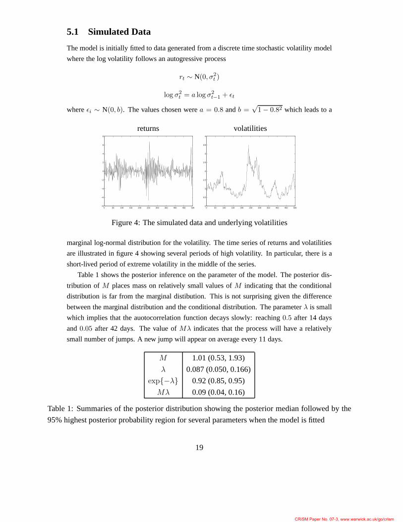
The model is initially fitted to data generated from a discrete time stochastic volatility model

where the log volatility follows an autogressive process

rt ∼ N(0, σ2t )

log σ2t = a log σ2

t−1 + εt

whereεi ∼ N(0, b). The values chosen werea = 0.8 andb =√

1 − 0.82 which leads to a

returns volatilities

0 50 100 150 200 250 300 350 400 450 500−8

−6

−4

−2

0

2

4

6

8

0 50 100 150 200 250 300 350 400 450 5000

0.5

1

1.5

2

2.5

3

3.5

4

Figure 4: The simulated data and underlying volatilities

marginal log-normal distribution for the volatility. The time series of returns and volatilities

are illustrated in figure 4 showing several periods of high volatility. In particular, there is a

short-lived period of extreme volatility in the middle of the series.

Table 1 shows the posterior inference on the parameter of themodel. The posterior dis-

tribution ofM places mass on relatively small values ofM indicating that the conditional

distribution is far from the marginal distibution. This is not surprising given the difference

between the marginal distribution and the conditional distribution. The parameterλ is small

which implies that the auotocorrelation function decays slowly: reaching0.5 after 14 days

and0.05 after 42 days. The value ofMλ indicates that the process will have a relatively

small number of jumps. A new jump will appear on average every11 days.

M 1.01 (0.53, 1.93)

λ 0.087 (0.050, 0.166)

exp{−λ} 0.92 (0.85, 0.95)

Mλ 0.09 (0.04, 0.16)

Table 1: Summaries of the posterior distribution showing the posterior median followed by the

95% highest posterior probability region for several parameters when the model is fitted

19


Smoothed and filtered estimates of the volatilities for these data are shown in figure 5.

Both estimates are able to capture the features of the changing volatility and clearly show the

periods of high volatility. The period of highest volatility in the middle of the series seems to

be a little shrunk. The filtered estimates are calculated using the particle filtering algorithm

2 conditional on the posterior median estimates ofλ andM . They behave in a similar way

to the smoother estimates but show some predictable difference. The median estimate is

similar to the smoothed estimate and gives a good indicationof the underlying changes in the

volatility.

filtered smoothed

Ft

0 50 100 150 200 250 300 350 400 450 5000

1

2

3

4

5

6

7

8

9

0 50 100 150 200 250 300 350 400 450 5000

1

2

3

4

5

6

7

8

9

σt

0 50 100 150 200 250 300 350 400 450 5000

1

2

3

4

5

6

7

8

9

0 50 100 150 200 250 300 350 400 450 5000

1

2

3

4

5

6

7

8

9

Figure 5: The filtered and smoothed estimates of the volatilities with the OUDP model for the

simulated data. The results are represented by the median (solid line) and the 2.5 and 97.5

percentile (dashed lines)

5.2 Brazilian stock exchange data

The Ibovespa index of the Brazilian stock exchange between 14/7/92 and 16/5/96 are plotted

in figure 6. The graph shows a period where the spread of returns is fairly constant upto

time 600 followed by a brief period of higher volatility followed by a longer period of low

volatility. Fitting the OUDP model to the data yields a posterior distribution ofM that is

similar to the simulated data example. However the parameter controlling dependenceλ is

estimated to be smaller indicating substantial correlation at longer times. The autocorrelation

20


0 100 200 300 400 500 600 700 800 900 1000−0.15

−0.1

−0.05

0

0.05

0.1

0.15

0.2

0.25

Figure 6: A time series graph of daily returns from the ibovespa index for the Brazilian stock

exchange

function equals 0.5 after 23 days and equals 0.05 afer 70 days. The posterior median estimate

of Mλ is also smaller with a new jump appearing every 18 days on average.

M 1.05 (0.54, 1.82)

λ 0.052 (0.029, 0.098)

exp{−λ} 0.95 (0.91, 0.97)

Mλ 0.055 (0.037, 0.079)

Table 2: A summary of the posterior distribution showing theposterior median followed by the

95% highest posterior probability region forM for the Ibovespa data

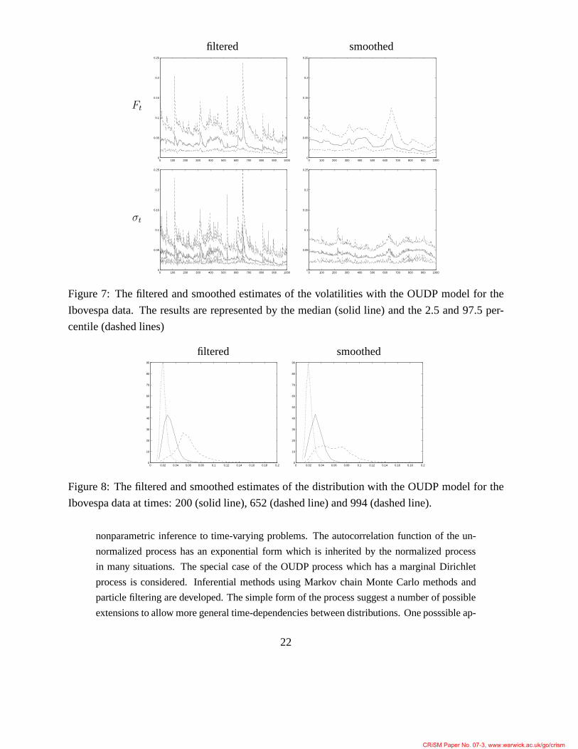
Figure 7 shows the smoothed and filtered results, which were calculated in the same ways

as with the simulated data. These graphs show the Fmain features of the volatility. An initial

constant period of volatility is followed by a period where the distribution of the volatility

becomes more widely spread. The results indicate that the right-hand tail of the distribution

increases alot (to capture the few large returns) which contrasts with the median value of

volatility that changes a much less pronounced way. The finalperiod of lower volatility is

captured.

Figure 8 shows the smoothed and filtered posterior distribution of volatility at several

selected time points. It shows that the distribution of volatility at several different time points

which indicates how the various periods of volatility are captured and show a substantial

variation in the fitted shapes.

6 Discussion

This paper has introduced a method for constructing stochastic processes with particular

marginal processes which generalize the Normalized RandomMeasures priors for Bayesian

21


filtered smoothed

Ft

0 100 200 300 400 500 600 700 800 900 10000

0.05

0.1

0.15

0.2

0.25

0 100 200 300 400 500 600 700 800 900 10000

0.05

0.1

0.15

0.2

0.25

σt

0 100 200 300 400 500 600 700 800 900 10000

0.05

0.1

0.15

0.2

0.25

0 100 200 300 400 500 600 700 800 900 10000

0.05

0.1

0.15

0.2

0.25

Figure 7: The filtered and smoothed estimates of the volatilities with the OUDP model for the

Ibovespa data. The results are represented by the median (solid line) and the 2.5 and 97.5 per-

centile (dashed lines)

filtered smoothed

0 0.02 0.04 0.06 0.08 0.1 0.12 0.14 0.16 0.18 0.20

10

20

30

40

50

60

70

80

90

0 0.02 0.04 0.06 0.08 0.1 0.12 0.14 0.16 0.18 0.20

10

20

30

40

50

60

70

80

90

Figure 8: The filtered and smoothed estimates of the distribution with the OUDP model for the

Ibovespa data at times: 200 (solid line), 652 (dashed line) and 994 (dashed line).

nonparametric inference to time-varying problems. The autocorrelation function of the un-

normalized process has an exponential form which is inherited by the normalized process

in many situations. The special case of the OUDP process which has a marginal Dirichlet

process is considered. Inferential methods using Markov chain Monte Carlo methods and

particle filtering are developed. The simple form of the process suggest a number of possible

extensions to allow more general time-dependencies between distributions. One posssible ap-

22


proach uses mixed OU processes (Barndorff-Nielsen, 2000) where the unnormalized process

is defined by

G?t =

∫

G?t (λ)µ(dλ)

whereG?t (λ) follows stochastic differential equation in (2) for a fixed value ofλ andµ is

a distribution. Inferential approach using MCMC methods have been considered by both

Robertet al (2004) and Griffin and Steel (2006b) whenG?(t) as a continuous-time volatil-

ity process andµ is a discrete distribution with a finite number of atoms, which could be

extended using some of the MCMC methods developed in this paper. Alternative general-

isations are explored by Gander and Stephens (2005) who apply the ideas of Wolpert and

Taqqu (2006) to stochastic volatility modelling. In particular they present alternative meth-

ods for defining a long-memory process. An interesting question for future research is “how

well can the autoocorrelation function be estimated from the data?”

The current work has concentrated on specifying known formsfor the process ofGt. An

alternative approach chooses a form for the background driving Levy process. The proper-

ties of the marginal process can then be derived. This approach can lead to simpler sampling

schemes in the stochastic volatility context. In particular James (2006) shows that the infinite

dimensional processG?(t) can be integrated from the process for particular choices. The

use of these models to define a time-varying normalized random measure seems an interest-

ing alternative approach to the ideas presented in this paper. The current work has focused

on Dirichlet process marginals since these processes have dominated the Bayesian nonpara-

metric literature. There has been recent work looking at other processes in applications. In

particular Teh (2006) considers the use of a Pitman-Yor process for language modelling. The

methods developed in this paper allow time-varying versions of such models and an interest-

ing direction for future work would be the exploration of non-Dirichlet process time-varying

models.

ReferencesAldous, D. (1983): “Exchangeability and related topics,” in L’Ecole d’ete de probabilites

de Saint-Flour, XIII-1983, Springer-Verlage, pgs 1-198.par

Barndorff-Nielsen, O. E. (2000): “Superposition of Ornstein-Uhlenbeck type processes,”

Theory of Probability and its Applications, 45, 175-194.

Barndorff-Nielsen, O. E. and Shephard, N. (2001): “Non-Gaussian Ornstein-Uhlenbeck

based models and some of their uses in financial economics (with discussion),”Journal

of the Royal Statistical Society B, 63, 167-241.

23


Bertoin, J. (1996): “Levy Processes,” Cambridge University Press: Cambridge.

Blackwell, D. and J. B. MacQueen (1973):“Ferguson distributions via Polya urn schemes,”

Annals of Statistics, 1, 353-355.

Caron, F., M. Davy, A. Doucet, E. Duflos and P. Vanheeghe (2006): “Bayesian Inference

for Linear Dynamic Models with Dirichlet Process Mixtures,” Technical Report.

Carpenter, J., P. Clifford and P. Fearnhead (1999): “An improved particle filter for non-

linear problems,”IEE proceedings - Radar, Sonar and Navigation, 146, 2-7.

Damien, P., J. Wakefield, and S. G. Walker (1999): “Gibbs sampling for Bayesian non-

conjugate and hierarchical models by using auxiliary variables,” Journal of the Royal

Statistical Society, B, 61, 331-344.

Doucet, A., N. de Freitas and N. Gordon (2001): “Sequential Monte Carlo Methods in

practice,” Springer-Verlag.

Escobar, M. D. and M. West (1995): “Bayesian Inference for Density Estimation,”Journal

of the American Statistical Assocation, 90, 577-588.

Fearnhead, P. (2003): “Particle filters for mixture models with an unknown number of

components,”Statistics and Computing, 14 , 11-21.

Ferguson, T. S. (1973): “A Bayesian analysis of some nonparametric problems,”Annals of

Statistics, 1, 209-230.

Ferguson, T. S. and Klass, M. J. (1972): “A representation ofindependent increment processes

without Gaussian components,”Annals of Mathematical Statistics, 43, 1634-43.

Gander, M. P. S. and D. A. Stephens (2005): “Inference for Stochastic Volatility Models

Driven by Levy Processes,”Technical Report, Imperial College London.

Gander, M. P. S. and D. A. Stephens (2006): “Stochastic Volatility Modelling with General

Marginal Distributions: Inference, Prediction and Model Selection For Option Pric-

ing,” Journal of Statistical Planning and Inference, to appear.

Griffin, J. E. and M. F. J. Steel (2006a): “Order-based Dependent Dirichlet Processes,”

Journal of the American Statistical Association, 101, 179-194.

Griffin, J. E. and M. F. J. Steel (2006b): “Inference with non-Gaussian OrnsteinUhlenbeck

processes for stochastic volatility,”Journal of Econometrics, 134, 605-644.

Ishwaran, H. and L. F. James (2001): “Gibbs Sampling Methodsfor Stick-Breaking Priors,”

Journal of the American Statistical Association, 96, 161-173.

Ishwaran, H. and James, L.F. (2003): “Some further developments for stick-breaking priors:

finite and infinite clustering and classification,”Sankhya Series A, 65, 577-592.

24


James, L. F., A. Lijoi and I. Prunster (2005): “Bayesian inference via classes of normalized

random measures,”Technical Report.

James, L. F. (2006): “Laws and likelihoods for Ornstein-Uhlenbeck Gamma and other BNS

OU Stochastic Volatility models with extensions,”Technical Report

Kingman, J. F. C. (1975): “Random discrete distributions,”Journal of the Royal Statistical

Society B, 37, 1-22.

Lijoi, A., R. H. Mena, and I. Prunster (2005): “Hierarchical mixture modelling with nor-

malized inverse-Gaussian priors,”Journal of the American Statistical Association, 100,

1278-1291./par

Lijoi, A., R. H. Mena, and I. Prunster (2006): “Controllingthe reinforcement in Bayesian

nonparametric mixture models,”Preprint

Liu, J. S. (1996): “Nonparametric hierarchical Bayes via sequential imputations,”Annals

of Statistics, 24, 911-930.

MacEachern, S. N., Clyde M. and Liu J. S. (1999): “Sequentialimportance sampling for

nonparametric Bayes models: The next generation,”Canadian Journal of Statistics,

27, 251-267.

Mallick, B. K. and S. G. Walker (1997): “Combining information from several experiments

with nonparametric priors,”Biometrika, 84, 697-706.

Mena. R. H. and Walker, S. G. : “Stationary Autoregresive Models via a Bayesian Non-

parametric Approach,”Journal of Time Series Analysis, 26, 789-805.

Muller, P. and Quintana, F. (2004): “Nonparametric Bayesian Data Analysis,”Statistical

Science, 19, 95-110.

Neal, R. M. (2003): “Slice sampling,”Annals of Statistics, 31, 705-767.

Papaspiliopoulos, O. and G. O. Roberts (2005): “Retrospective Markov chain Monte Carlo

methods for Dirichlet process hierarchical models,”Technical Report, University of

Lancaster.

Pennell, M.L. and Dunson, D.B. (2005): “Bayesian semiparametric dynamic frailty models

for multiple event time data,”Biometrics, to appear.

Pitman, J. and Yor, M. (1997): “The two-parameter Poisson-Dirichlet distribution derived

from a stable subordinator,”Annals of Probability, 25, 855-900.

Regazzini, E., A. Lijoi and I. Prunster (2003): “Distributional results for means of nor-

malized random measures with independent increments.”The Annals of Statistics, 31,

560-585.

25


Roberts, G. O., O. Papaspiliopoulos and P. Dellaportas (2004): “Bayesian inference for

Non-Gaussian Ornstein-Uhlenbeck Stochastic Volatility models,”Journal of the Royal

Statistical Society B, 66, 369-393.

Sato, K. (1999): “Levy Processes and Infinitely Divisible Distributions,” CUP : Cambridge.

Shephard, N. (2005): “Stochastic Volatility: Selected Reading,” OUP : Oxford.

Taylor, S. J. (1986): “Modelling Financial Time Series” John Wiley and Sons : Chichester.

Teh, Y. W. (2006): “A Hierarchical Bayesian Language Model based on Pitman-Yor process,”

Technical Report.

Tsay, R. (2005): “Analysis of Financial Time Series,” Wiley.

Wolpert, R. L. and M. Taqqu (2006): “Fractional Ornstein-Uhlenback Levy Processes and

the Telecom Process: Upstairs and Downstairs,”Signal Processing, to appear.

Zhu, X., Ghahramani, Z., and Lafferty, J. (2005): “Time-Sensitive Dirichlet Process Mix-

ture Models,” Carnegie Mellon University Technical ReportCMU-CALD-05-104.

A Proofs

A.1 Proof of theorem 1

We need to show thatG?t =

∑∞i=1 I(τi ≤ t) exp{−λ(t − τi)}Jiδθi

follows the appropriate

unnormalized Levy process. Consider a measureable setB thenG?t (B) =

∑∞i=1 I(τi ≤

t) exp{−λ(t − τi)}Jiδθi(B) which is an independent thinning ofG?(S) =

∑∞i=1 I(τi ≤

t) exp{−λ(t−τi)}Jiδθi(S) with thinning probabilityH(B). Therefore it has the same distri-

bution as∑∞

i=1 I(τ?i ≤ t) exp{−λ(t−τ?

i )}J?i where(τ?, J?) is a Poisson processR+×R

+

which has intensityW+(J)H(B)λ which by the properties of the BNS construction has the

marginal distributionW+(J)H(B), which is the marginal distribution of the unnormalized

measure onB under the NRM(W+,H).

A.2 Proof of result 1

Cov(Gt, Gt+k) = Cov

(

G?t (B)

G?t (B) +G?

t (S\B),

exp{−λt}G?t (B) +

∑ki=1 exp{−λti}Jiδθi

(B)

exp{−λt}G?t (S) + exp{−λt}G?

t (S\B) +∑k

i=1 exp{−λti}Ji

)

Cov(Gt, Gt+k) = Cov

(

Gt(B),exp{−λt}G?

t (S)Gt(B) +H(B)∑k

i=1 exp{−λti}Ji

exp{−λt}G?t (S) +

∑ki=1 exp{−λti}Ji

)

E(GtGt+k) = E

(

exp{−λt}G?t (S)Gt(B)2 +Gt(B)H(B)




)

26


Cov(Gt, Gt+k) = E

(

exp{−λt}G?t (S)Gt(B)2 +Gt(B)H(B)




)

−H(B)2

Cov(Gt, Gt+k) = E

(

G?t (S)Gt(B)2 +Gt(B)H(B)

∑ki=1 exp{−λ(ti − t)}Ji



)

−H(B)2

Asymptotically

exp{λt}Cov(Gt, Gt+k) = E

(

G?t (S)Gt(B)2 +Gt(B)H(B) exp{λt}∑k

i=1 exp{−λti}Ji∑k

i=1 exp{−λti}Ji

)

−H(B)2


(

G?t (S)G?

t (B)2∑k

i=1 exp{−λti}Ji

)

+ exp{λt}H(B)2 exp{λt} −H(B)2


(

G?t (S)Gt(B)2


)

The autocorrelation is asymptotically

E

(

G?t (S)Gt(B)2


)

exp{−λt}

A.3 Derivation of autocorrelation for OUDP

The general result

g(X,Y ) =X

Y

E[Z] =E[X]

E[Y ]+ σ2

Y

E[X]

E[Y ]3− σXY

1

E[Y ]2

then E[X] = exp{−λ∆}µ and E[Y ] = µ by stationarity whereµ = E[G(X )]. Cov(X,Y ) =

Cov(X,X) + Cov(X,Y −X) = V(X) = exp{−2λ∆}σ2 whereσ2 = V[G?(S)].

E[Z] = exp{−λ∆}[

1 +σ2

µ2(1 − exp{−λ∆})

]

for the Dirichlet processσ2

µ2 = 1M

27


Documents

The Ornstein-Uhlenbeck Dirichlet Process and other time