Applications Of Ornstein-Uhlenbeck Type Stochastic

University of Texas at El Paso University of Texas at El Paso

ScholarWorks@UTEP ScholarWorks@UTEP

Open Access Theses & Dissertations

2020-01-01

Applications Of Ornstein-Uhlenbeck Type Stochastic Differential Applications Of Ornstein-Uhlenbeck Type Stochastic Differential

Equations Equations

Osei Kofi Tweneboah University of Texas at El Paso

Follow this and additional works at: https://scholarworks.utep.edu/open_etd

Part of the Applied Mathematics Commons, and the Statistics and Probability Commons

Recommended Citation Recommended Citation Tweneboah, Osei Kofi, "Applications Of Ornstein-Uhlenbeck Type Stochastic Differential Equations" (2020). Open Access Theses & Dissertations. 3052. https://scholarworks.utep.edu/open_etd/3052

This is brought to you for free and open access by ScholarWorks@UTEP. It has been accepted for inclusion in Open Access Theses & Dissertations by an authorized administrator of ScholarWorks@UTEP. For more information, please contact [email protected].

https://scholarworks.utep.edu/

https://scholarworks.utep.edu/open_etd

https://scholarworks.utep.edu/open_etd?utm_source=scholarworks.utep.edu%2Fopen_etd%2F3052&utm_medium=PDF&utm_campaign=PDFCoverPages

http://network.bepress.com/hgg/discipline/115?utm_source=scholarworks.utep.edu%2Fopen_etd%2F3052&utm_medium=PDF&utm_campaign=PDFCoverPages

http://network.bepress.com/hgg/discipline/208?utm_source=scholarworks.utep.edu%2Fopen_etd%2F3052&utm_medium=PDF&utm_campaign=PDFCoverPages

https://scholarworks.utep.edu/open_etd/3052?utm_source=scholarworks.utep.edu%2Fopen_etd%2F3052&utm_medium=PDF&utm_campaign=PDFCoverPages

mailto:[email protected]

APPLICATIONS OF ORNSTEIN-UHLENBECK TYPE STOCHASTIC DIFFERENTIAL

EQUATIONS

OSEI KOFI TWENEBOAH

Doctoral Program in Computational Science

APPROVED:

Maria Christina Mariani, Ph.D., Chair

Granville Sewell, Ph.D.

Thompson Sarkodie-Gyan, Ph.D.

Kristine Garza, Ph.D.

Stephen Crites, Ph.D.Dean of the Graduate School

c©Copyright

by

Osei Kofi Tweneboah

2020

This Dissertation is dedicated to my parents

John Tweneboah

and

Christiana Tweneboah

with love

APPLICATIONS OF ORNSTEIN-UHLENBECK TYPE STOCHASTIC DIFFERENTIAL

EQUATIONS

by

OSEI KOFI TWENEBOAH, B.S., M.S.

DISSERTATION

Presented to the Faculty of the Graduate School of

The University of Texas at El Paso

in Partial Fulfillment

of the Requirements

for the Degree of

DOCTOR OF PHILOSOPHY

Computational Science Program

THE UNIVERSITY OF TEXAS AT EL PASO

May 2020

Acknowledgements

My sincere appreciation goes to the Almighty God for his love, mercy and abundant grace

shown me throughout my education.

I would like to express my deep-felt gratitude to my advisor and chair of the Mathematical

Sciences Department at The University of Texas at El Paso, Dr. Maria Christina Mariani for

her mentoring, advice, encouragement, enduring patience and keen interest which brought

my dissertation to a successful completion.

I also wish to thank the other members of my committee, Dr. Granville Sewell of the Math-

ematical Sciences Department and Computational Science Program, Dr. Thompson Sarkodie-

Gyan of the Electrical & Computer Engineering Department and Dr. Kristine Garza of the

Biological Sciences Department all at The University of Texas at El Paso. Their suggestions,

comments and additional guidance were invaluable to the completion of this work.

I want to thank Dr. Hector Gonzalez-Huizar for his suggestions and providing me with the

geophysical data and Dr. Ionut Florescu for providing me with the high frequency financial

time series.

I also want to thank The University of Texas at El Paso Computational Sciences Program

and Mathematical Sciences Department professors and staff for all their hard work and dedi-

cation, providing me the means to complete my degree.

My warmest gratitude also goes to my dear parents and wife for their love, encouragement

and constant support. I say God richly bless you.

And finally, I extend my sincere thanks to all colleagues, friends and loved ones who

contributed in various ways to make this work a success.

v

Abstract

In this dissertation, we show with plausible arguments that the Stochastic Differential Equa-

tions (SDEs) arising on the superposition and coupling system of independent Ornstein-

Uhlenbeck process is a new method available in modern literature that takes the properties

and behavior of the data into consideration when performing the statistical analysis of the

time series.

The time series to be analyzed is thought of as a source of fluctuations, and thus we need a

model that takes this behavior into consideration when performing such analysis. Most of the

standard methods fail to take into account the physical behavior of the time series, and some

of the models are not completely stochastic. Thus in an attempt to overcome the modeling

problems associated with the memory-less property models used in the traditional methods,

we propose a continuous-time stationary and non-negative stochastic differential equation that

is useful for describing a unique type of dependence in a sequence of events.

The Ornstein-Uhlenbeck type SDE offers plenty of analytic flexibility which is not avail-

able to more standard models such as the geometric Gaussian Ornstein-Uhlenbeck processes.

Moreover, the SDE provides a class of continuous time processes capable of exhibiting long

memory behavior. The presence of long memory suggests that current information is highly

correlated with past information at different levels. This facilitates prediction.

The proposed SDE is applied to two different sets of real data; financial and geophysical

time series. In the analysis of the time series, we show that the SDE makes new properties

and estimate parameters that are useful for making inferences and predicting these types of

events.

vi

Table of Contents

Page

Acknowledgements . . . . . . . . . . . . . . . . . . . . . . . . . . . . . . . . . . . . . . . . . v

Abstract . . . . . . . . . . . . . . . . . . . . . . . . . . . . . . . . . . . . . . . . . . . . . . . vi

Table of Contents . . . . . . . . . . . . . . . . . . . . . . . . . . . . . . . . . . . . . . . . . . vii

List of Tables . . . . . . . . . . . . . . . . . . . . . . . . . . . . . . . . . . . . . . . . . . . . . xi

List of Figures . . . . . . . . . . . . . . . . . . . . . . . . . . . . . . . . . . . . . . . . . . . . xii

Chapter

1 Introduction . . . . . . . . . . . . . . . . . . . . . . . . . . . . . . . . . . . . . . . . . . . 1

2 Stochastic Processes and Stochastic Differential Equations . . . . . . . . . . . . . . . . 8

2.1 Necessary definitions from probability theory . . . . . . . . . . . . . . . . . . . . 8

2.2 Stochastic Processes . . . . . . . . . . . . . . . . . . . . . . . . . . . . . . . . . . . 11

2.2.1 The Index Set I . . . . . . . . . . . . . . . . . . . . . . . . . . . . . . . . . . 11

2.2.2 The State Space S . . . . . . . . . . . . . . . . . . . . . . . . . . . . . . . . . 11

2.2.3 Stationary and Independent Components . . . . . . . . . . . . . . . . . . . 12

2.2.4 Stationary and Independent Increments . . . . . . . . . . . . . . . . . . . . 13

2.2.5 Filtration and Standard Filtration . . . . . . . . . . . . . . . . . . . . . . . 14

2.2.6 Time series . . . . . . . . . . . . . . . . . . . . . . . . . . . . . . . . . . . . . 15

2.3 Examples of stochastic processes . . . . . . . . . . . . . . . . . . . . . . . . . . . . 18

2.3.1 Markov processes . . . . . . . . . . . . . . . . . . . . . . . . . . . . . . . . . 19

2.3.2 Martingales . . . . . . . . . . . . . . . . . . . . . . . . . . . . . . . . . . . . 19

2.3.3 Simple random walk . . . . . . . . . . . . . . . . . . . . . . . . . . . . . . . 20

2.3.4 The Brownian Motion (Wiener process) . . . . . . . . . . . . . . . . . . . . 20

2.4 Levy Processes . . . . . . . . . . . . . . . . . . . . . . . . . . . . . . . . . . . . . . 21

2.4.1 Properties of Levy Processes . . . . . . . . . . . . . . . . . . . . . . . . . . 24

2.5 Examples of Levy Processes . . . . . . . . . . . . . . . . . . . . . . . . . . . . . . . 25

vii

2.5.1 Poisson Process . . . . . . . . . . . . . . . . . . . . . . . . . . . . . . . . . . 25

2.5.2 Compound Poisson Process . . . . . . . . . . . . . . . . . . . . . . . . . . . 26

2.5.3 The Gamma Process . . . . . . . . . . . . . . . . . . . . . . . . . . . . . . . 27

2.5.4 Inverse Gaussian Process . . . . . . . . . . . . . . . . . . . . . . . . . . . . 28

2.6 Subordination of Levy processes . . . . . . . . . . . . . . . . . . . . . . . . . . . . 28

2.7 Deterministic Differential Equations . . . . . . . . . . . . . . . . . . . . . . . . . . 29

2.8 Ito Integrals . . . . . . . . . . . . . . . . . . . . . . . . . . . . . . . . . . . . . . . . 31

2.8.1 Properties of the Ito integral . . . . . . . . . . . . . . . . . . . . . . . . . . 34

2.9 Ito Lemma . . . . . . . . . . . . . . . . . . . . . . . . . . . . . . . . . . . . . . . . . 35

2.10 One-dimensional Stochastic Differential Equation . . . . . . . . . . . . . . . . . . 39

2.10.1 An Existence and Uniqueness Result . . . . . . . . . . . . . . . . . . . . . 40

2.10.2 Weak and Strong Solutions . . . . . . . . . . . . . . . . . . . . . . . . . . . 41

2.11 Multi-dimensional Stochastic Differential Equations . . . . . . . . . . . . . . . . . 42

2.12 Simulation of stochastic differential equations . . . . . . . . . . . . . . . . . . . . 43

2.12.1 Euler–Maruyama scheme for approximating stochastic differential equa-

tions . . . . . . . . . . . . . . . . . . . . . . . . . . . . . . . . . . . . . . . . 44

2.12.2 Euler–Milstein scheme for approximating stochastic differential equations 46

3 Construction of Ornstein-Uhlenbeck type Stochastic Differential Equation . . . . . . . 49

3.1 Introduction . . . . . . . . . . . . . . . . . . . . . . . . . . . . . . . . . . . . . . . . 49

3.2 One-dimensional Ornstein-Uhlenbeck Processes . . . . . . . . . . . . . . . . . . . 51

3.2.1 Solution of the One-dimensional Ornstein-Uhlenbeck Processes . . . . . 51

3.2.2 Superposition of the Ornstein-Uhlenbeck Processes . . . . . . . . . . . . . 52

3.3 Multi-dimensional Ornstein-Uhlenbeck Processes . . . . . . . . . . . . . . . . . . 53

3.3.1 Solution of the Multi-dimensional Ornstein-Uhlenbeck Processes . . . . . 54

3.4 Levy density and the tail mass function . . . . . . . . . . . . . . . . . . . . . . . . 59

3.5 Parameter Estimation of the one-dimensional Γ(a, b) Ornstein-Uhlenbeck type

Model . . . . . . . . . . . . . . . . . . . . . . . . . . . . . . . . . . . . . . . . . . . . 63

viii

3.5.1 Estimation of the shape parameter a and rate parameter b of the Γ(a, b)

Ornstein-Uhlenbeck Model . . . . . . . . . . . . . . . . . . . . . . . . . . . 63

3.5.2 Estimation of the intensity parameter λ1 of the Γ(a, b) Ornstein-Uhlenbeck

Model . . . . . . . . . . . . . . . . . . . . . . . . . . . . . . . . . . . . . . . 64

3.6 Parameter Estimation of the 2-dimensional Γ(a, b) Ornstein-Uhlenbeck type Model 65

3.7 Simulation techniques . . . . . . . . . . . . . . . . . . . . . . . . . . . . . . . . . . 65

3.7.1 Simulation of the 1-dimensional stochastic model via the background

driving Levy process . . . . . . . . . . . . . . . . . . . . . . . . . . . . . . . 66


driving Levy process . . . . . . . . . . . . . . . . . . . . . . . . . . . . . . . 66

4 Stochastic differential equations applied to the study of financial time series . . . . . 68

4.1 Introduction . . . . . . . . . . . . . . . . . . . . . . . . . . . . . . . . . . . . . . . . 68

4.2 Background of Financial Time Series . . . . . . . . . . . . . . . . . . . . . . . . . . 70

4.3 Numerical Simulation and Results . . . . . . . . . . . . . . . . . . . . . . . . . . . 72

4.3.1 Real Data Analysis of the Financial Indices . . . . . . . . . . . . . . . . . . 72

4.4 Concluding remarks . . . . . . . . . . . . . . . . . . . . . . . . . . . . . . . . . . . 74

5 Analysis of high frequency financial time series by using a stochastic differential

equation . . . . . . . . . . . . . . . . . . . . . . . . . . . . . . . . . . . . . . . . . . . . . 77

5.1 Introduction . . . . . . . . . . . . . . . . . . . . . . . . . . . . . . . . . . . . . . . . 77

5.2 Background of the High Frequency Financial Time Series . . . . . . . . . . . . . 78

5.3 Analysis of the High Frequency Financial Time Series . . . . . . . . . . . . . . . . 79

5.4 Significance of the results obtained . . . . . . . . . . . . . . . . . . . . . . . . . . . 83

6 Stochastic Differential Equation of Earthquakes Series . . . . . . . . . . . . . . . . . . . 84

6.1 Introduction . . . . . . . . . . . . . . . . . . . . . . . . . . . . . . . . . . . . . . . . 84

6.2 Earthquake Time Series . . . . . . . . . . . . . . . . . . . . . . . . . . . . . . . . . 85

6.3 Numerical Simulation and Results . . . . . . . . . . . . . . . . . . . . . . . . . . . 87

6.3.1 Results from analysis of earthquake time series . . . . . . . . . . . . . . . 88

6.4 Significance of the results obtained . . . . . . . . . . . . . . . . . . . . . . . . . . . 89

ix

7 Modeling earthquake series dependencies by using coupled system stochastic differ-

ential equations . . . . . . . . . . . . . . . . . . . . . . . . . . . . . . . . . . . . . . . . . 93

7.1 Background of Earthquake Time Series . . . . . . . . . . . . . . . . . . . . . . . . 94

7.2 Application . . . . . . . . . . . . . . . . . . . . . . . . . . . . . . . . . . . . . . . . 96

7.3 Results . . . . . . . . . . . . . . . . . . . . . . . . . . . . . . . . . . . . . . . . . . . 97

7.4 Concluding remarks . . . . . . . . . . . . . . . . . . . . . . . . . . . . . . . . . . . 102

8 Conclusion . . . . . . . . . . . . . . . . . . . . . . . . . . . . . . . . . . . . . . . . . . . . 103

References . . . . . . . . . . . . . . . . . . . . . . . . . . . . . . . . . . . . . . . . . . . . . . 106

Appendix

Curriculum Vitae . . . . . . . . . . . . . . . . . . . . . . . . . . . . . . . . . . . . . . . . . . 112

x

List of Tables

2.1 Examples of random variables . . . . . . . . . . . . . . . . . . . . . . . . . . . . . 10

2.2 Moments of the Poisson distribution with intensity λ . . . . . . . . . . . . . . . . 26

2.3 Moments of the Γ(a, b) distribution . . . . . . . . . . . . . . . . . . . . . . . . . . 28

4.1 Estimation of Parameters: λ1, a, b. . . . . . . . . . . . . . . . . . . . . . . . . . . . . 73

4.2 Numerical results for the superposed Γ(a, b) Ornstein-Uhlenbeck model. . . . . 73

4.3 Numerical results for the Γ(a, b) Ornstein-Uhlenbeck model. . . . . . . . . . . . . 73

5.1 Estimation of Parameters for the minute-by-minute sampled data: λ1, a, b . . . . 81

5.2 Estimation of Parameters for the second-by-second sampled data: λ1, a, b. . . . . 82

5.3 Numerical results of the stochastic model for minute-by-minute sample data. . . 82

5.4 Numerical results of the stochastic model for second-by-second data. . . . . . . 82

5.5 Comparison of the numerical results of the minute and second data. . . . . . . . 82

6.1 Coordinates of the four study regions. . . . . . . . . . . . . . . . . . . . . . . . . . 85

6.2 Estimation of Parameters: λ1, a, b. . . . . . . . . . . . . . . . . . . . . . . . . . . . . 88

6.3 Data Results for superposed Γ(a, b) Ornstein-Uhlenbeck model. . . . . . . . . . . 88

6.4 Data Results for Γ(a, b) Ornstein-Uhlenbeck model. . . . . . . . . . . . . . . . . . 89

7.1 Data and parameter estimates . . . . . . . . . . . . . . . . . . . . . . . . . . . . . . 97

7.2 Data Results for 2-dimensional Γ(a, b) Ornstein-Uhlenbeck model. . . . . . . . . 98

xi

List of Figures

2.1 The time series data of arrival phased from earthquake occurring on 7/26/14. . 16

2.2 Time series data of financial returns from Bank of America (BAC) stock index. . 17

4.1 The closing prices of daily trading observations from the BVSP stock exchange. 71

4.2 The closing prices of daily trading observations from the S&P 500 stock exchange. 71

4.3 Sample Path of the BOVESPA financial index. . . . . . . . . . . . . . . . . . . . . 74

4.4 Sample Path of the MERVAL financial index. . . . . . . . . . . . . . . . . . . . . . 75

4.5 Sample Path of the HSI financial index. . . . . . . . . . . . . . . . . . . . . . . . . 75

4.6 Sample Path of the S&P 500 financial index. . . . . . . . . . . . . . . . . . . . . . 76

5.1 The return values within minute-by-minute for the BAC stock exchange. . . . . 79

5.2 The return values within second-by-second for the BAC stock exchange. . . . . . 79

5.3 The return values within minute-by-minute for the DIS stock exchange. . . . . . 80

5.4 The return values within second-by-second for the DIS stock exchange. . . . . . 80

5.5 The return values within minute-by-minute for the JPM stock exchange. . . . . . 81

5.6 The return values within second-by-second for the JPM stock exchange. . . . . . 81

6.1 Magnitude as a function of time origin of earthquakes for the 4 study regions

defined in Table 6.1. . . . . . . . . . . . . . . . . . . . . . . . . . . . . . . . . . . . 86

6.2 A Sample Path of the superposed Γ(a, b)-OU process with λ1 = 2.1776, λ2 =

2.9776 , a = 158.9808 and b = 34.4993 for region 1. . . . . . . . . . . . . . . . . . . 90


4.6165 , a = 196.4128 and b = 43.2430 for region 2. . . . . . . . . . . . . . . . . . . 90


2.3348 , a = 151.7649 and b = 33.0730 for region 3. . . . . . . . . . . . . . . . . . . 91

xii


2.6344 , a = 205.7332 and b = 46.0565 for region 4. . . . . . . . . . . . . . . . . . . 91

7.1 Map shows the spatial distribution of earthquakes (colored circles) along the

tectonic boundary (red line) between the Nazca and the South American tectonic

plates. Red rectangles represent the four study regions. Inset shows the area

in larger map. Color represents earthquake’s depths. White circles mark the

location of the very large earthquakes (Mw≥8). For reference, white star marks

the location of the largest earthquake ever recorded. . . . . . . . . . . . . . . . . 95

7.2 Sample Path of the coupled stochastic model for regions 1 and 2. . . . . . . . . . 99






xiii

Chapter 1

Introduction

Most areas of science rely on Big Data and correctly modeling these data will help answer

some of the key research questions in data science, statistics and related fields. Big data is a

term applied to ways to analyze, extract information from, or otherwise deal with data sets

that are too large or complex to be dealt with by classical data-processing application software.

Big data has one or more of the following characteristics: high volume, high velocity, high

variety and high veracity. That is the data sets are characterized by huge amounts (volume)

of frequently updated data (velocity) in various types, such as numeric, textual, audio, images

and videos (variety) with high quality (veracity).

The objective of this dissertation is to introduce a new method to enhance the understand-

ing of “extreme events” in data science, statistics and related fields. The main interest is

verifying using theoretical and practical framework that our proposed new method describes

accurately the behavior of financial indices and earthquake series. We show with plausible

arguments that the stochastic differential equations arising on the superposition and coupling

system of independent Ornstein-Uhlenbeck process is a new method available in modern lit-

erature that takes the physical behavior of the data into consideration when modeling and

performing the statistical analysis of the time series. In the paragraphs that follow, we will re-

view some literature that have been dedicated to the modeling of complex data sets in finance

and geophysics.

In recent years, due to the huge amount of data available in the financial market, there has

been a constant interest by researchers and practitioners to develop models to describe these

data sets. Modeling and analyzing these financial sampled data helps investors, practitioners

and researchers make useful inference and predictions. The financial data mentioned are data

1

sets that are related to stock market crashes. A stock market crash is a sudden decline of

stock prices across a significant cross-section of a stock market, resulting in a significant loss

of paper wealth. Market crashes are often influenced by panic as much as by underlying

economic factors [58]. There has been a growing literature in financial economics analyzing

the behavior of major stock indices. Most of these literature are based on deterministic and

probabilistic models to depict various aspects of the mathematical and statistical modeling

of major stock indices. In deterministic models, the output of the model is fully determined

by the initial conditions and parameter values. On the other hand, stochastic models possess

some intrinsic randomness, that is, the same set of initial conditions and parameter values will

lead to a group of different outputs.

One of the first models developed for describing the evolution of stock prices is the Brow-

nian motion. This model assumes that the increment in the logarithm of the prices follows a

diffusive process with Gaussian distribution [59]. However, the empirical study of some finan-

cial indices shows that in the short time intervals the associated probability density function

has greater kurtosis than a Gaussian distribution [30], and that the Brownian motion does not

describe correctly the evolution of financial indices near a market crash. The authors in Refs.

[30], [35] and [33] tried to overcome this issue by using a stable non-Gaussian Levy process

that takes into account the long correlation scales. To be specific, the authors in Ref. [30]

proved that the scaling of the probability distribution of a Standard & Poor’s 500 stock index

can be described by a non-Gaussian process with dynamics that, for the central part of the

distribution, correspond to a Levy stable process. Also in the work by Ref. [35], the authors

studied the statistical properties of financial indices from developed and emergent markets.

They performed the analysis of different financial indices near a crash for both developed and

emergent markets by using a normalized truncated Levy walk model. Later the authors in

Ref. [33], studied the correlations, memory effects and other statistical properties of several

stocks. The authors verified that the behaviors of the stock returns were compatible with that

of continuous time Levy processes. Furthermore the authors concluded that stochastic volatil-

ity models, jump diffusion models and general Levy processes are useful for the modeling of

2

financial time series. Other researchers also described and modeled the behavior of a financial

market before a crash by analyzing high frequency financial sampled data (see [31], [6] and

[10]). For example, by using the Ising type model the authors in Ref. [31] studied high fre-

quency market data leading to the Bear Stearns crash [18] which occurred in mid March 2008.

They predicted the time when stock prices experience phase transition. A phase transition is

a change in state from one phase to another. In this context, the two states are buy and sell.

Thus if all traders decision changes from a buy and aligned to a sell phenomenon this leads

to a market crash.

Next, we review some literature that have been used to describe geophysical data specif-

ically earthquake time series. As the knowledge of the geophysical mechanisms that drive

seismic events have increased, so have the corresponding mathematical and statistical model

representations. In fact a good estimation of the seismic hazard in a region requires the pre-

diction of time, location and magnitude of future seismic events [37].

As in the modeling of stock indices, in geophysics several deterministic and probabilistic

models have been studied to describe the temporal evolution of earthquake sequences. Prob-

abilistic models such as the long term correlations have been applied to the occurrences of

seismic events (see [29]). In Ref. [29] the authors showed that the long term correlations can

explain both the fluctuations of magnitudes and their interoccurrence times in the seismic

records. In a different study, the authors in Ref. [44] used a stochastic finite fault source model

to estimate ground motion in northeastern India for intermediate depth events originating in

the Indo-Burmese tectonic domain. Accelerograms from eight events with magnitudes rang-

ing from Mw 4.8 − 6.4 were used to estimate the input source and site parameters of the

stochastic finite fault source model. Stochastic modeling of the ground acceleration due to

an earthquake using an existing deterministic formulation was presented by Ref. [15]. The

author constructed a non-stationary stochastic model by making use of the well-known ω

square model for source time function of the earthquake. The author argued that, the result of

applying this procedure is a model whose main parameter has a physical interpretation, and

therefore a validation based on criteria other than statistical goodness of fit is also possible.

3

The authors in Ref. [60] proposed a stochastic differential equation (SDE) to simulate Group

Delay Time (GDT) of earthquake ground motion. They expressed the random characteristic

of the GDT using the SDE whose mean and variance processes where defined by ordinary

differential equations and solved the SDE of GDT using the Milstein approximation scheme.

In their work, the efficiency of the developed model was demonstrated by comparing the

simulated results with the original one. The most interesting model in recent time has been

the scale invariant functions and Levy models which have been used to estimate parameters

related to some major events [34]. In this study the authors, by looking at the preceding data

collected before a major earthquake estimated the parameters leading to these critical events.

The modeling approach used was similar to [31], where they described the behavior of the

market before a financial crash.

Most of the models reviewed above have in common the fact that they are based upon

the Gaussian assumption, that is, we can describe the behavior of the time series by studying

the variance of the generated diffusion process. This fact is not completely accurate because

empirical study [30] of some financial stock indices suggests that the Gaussian assumption is

typically inappropriate because asset returns often exhibit excess kurtosis and asymmetries

[4]. Furthermore, most of the models described in previous literature fails to take into account

the physical behavior of the financial and earthquake data, and some of the models are not

completely stochastic. As in reality many phenomena are influenced by random noise, behav-

ior of the noise should be reflected in the model [25]. Therefore there is the need to understand

the general principles of the mathematical and statistical modeling of datasets which describes

the actual realizations.

In an attempt to overcome the modeling problems associated with the memory-less prop-

erty models described in previous literature and also incorporate the physical behavior of the

time series, we propose a continuous-time stationary and non-negative stochastic differential

equation that is useful in describing a unique type of dependence in a sequence of events. In

finance and econometrics, this stochastic model accounts for the stochastic nature of both the

process of price fluctuations and the process of trade durations [23]. Continuous-time stochas-

4

tic volatility models are now popular ways to describe many “critical phenomena” because of

their flexibility in accommodating most stylized facts of time series data such as moderate and

high frequency data. The authors in Ref. [9] proposed a class of models where the volatility

behaved according to an Ornstein-Uhlenbeck process driven by a positive Levy process with

a non-Gaussian component. This model type has many applications in many fields of science

and other disciplines [51]. There are also known applications within the context of finance and

econometric [9]. The Ornstein-Uhlenbeck process is a mean reverting process which is widely

used for modeling interest rates and commodities among many others.

In this dissertation, we implement very flexible classes of processes that incorporate long-

range dependence, that is, they have a slowly polynomially decaying autocovariance function

and self-similarity like properties that are capable of describing some of the key distribu-

tional features of typical financial and geophysical time series . In order to capture realistic

dependence structures, we combine and couple system of independent Ornstein-Uhlenbeck

processes driven by a Γ(a, b) process which is a Levy process. This selection is supported

by the fact that generalized Levy models are suitable for describing these type of time se-

ries, see [34]. The advantage of the superposition and coupling system of independent Γ(a, b)

Ornstein-Uhlenbeck processes is that it offers plenty of analytic flexibility which is not avail-

able for more standard models such as the geometric Gaussian Ornstein-Uhlenbeck processes.

Moreover, superposition of Ornstein-Uhlenbeck processes provide a class of continuous time

processes capable of exhibiting long memory behavior. The presence of long memory suggests

that current information is highly correlated with past information at different levels. This fa-

cilitates prediction. The methodology used in this work can be applied to other disciplines

such as biology, bioinformatics, medicine and in social sciences.

The dissertation is organized in two parts followed by a conclusion. The first part addresses

the theory of Stochastic Processes and Stochastic Differential Equations and the numerical sim-

ulations that verify the theoretical results. The second part shows applications of the model to

real data. Each application addresses a particular way to work with the Stochastic Differential

5

Equations for describing the behavior of financial and geophysical time series.

Chapter 2 reviews the necessary definitions from probability theory, stochastic and Levy

processes. We will also discuss the Γ(a, b) distribution and provide a detail description and

definitions of a stochastic differential equation and its solution methods.

In Chapter 3 we discuss the non Gaussian Ornstein-Uhlenbeck processes in detail, derive

some important results and pave the way for the proposed superposed and coupled Γ(a, b)

Ornstein-Uhlenbeck model. The main characteristic of the proposed stochastic model will

be discussed and shown. Simulation methods to generate realizations of the model are also

presented.

The results illustrated from Chapters 4 to the end are original results of this dissertation

and have produced several papers, some already published ([37, 36, 32]) and more publications

are expected to results from this dissertation.

The second part of the dissertation begins with Chapter 4 in which the stochastic differ-

ential equations is applied to the study of well developed and emergent market indices. For

the time series arising on financial indices near a crash for both well developed and emergent

markets, we estimate the daily closing values. Chapter 5 is dedicated to analyzing using a

stochastic differential equation the second-by-second and minute-by-minute sampled financial

data from the Bear Stearns companies and estimating parameters that are useful for making

inferences and predicting these types of events. This results may help an investor or practi-

tioner who lacks insider information but has at their disposal all the information contained in

the equity prices discover that a crash is imminent and take the necessary precautions.

Chapter 6 is dedicated to the modeling of earthquake series. An important example and

potential application of this work is for analyzing the effect of events that occurred very far

in the past, for example decades ago, might have on the occurrence of present and future

events. This type of analysis might help to better understand how tectonic stress decays and

accumulates during long period of time. Chapter 7 is dedicated to describing the effects

of geophysical time series arising between different regions in the same geographical area

6

by using coupled systems of stochastic differential equations. The objective is to model the

correlation and effects of earthquake series occurring at different regions.

The dissertation ends with a short conclusion and with a research project concerning fur-

ther applications of this methodology.

7

Chapter 2

Stochastic Processes and Stochastic

Differential Equations

This chapter is divided into two parts. The first part describes the theory of stochastic pro-

cesses and the second is dedicated to the theory of stochastic differential equations. In the

first part of this chapter we give definitions, properties and examples of stochastic processes

that will be useful throughout this dissertation. In the second part, we will discuss in detail

stochastic differential equations and their solution methods.

Stochastic processes and stochastic differential equations play a fundamental role in Math-

ematical Finance, as well as other fields of science, such as Physics (turbulence), Engineer-

ing (telecommunications, dams), Actuarial Science (insurance risk) and several others. Gen-

eral reference works on stochastic processes and stochastic differential equations are given by

[43],[48],[49],[50],[47] and [2].

2.1 Necessary definitions from probability theory

We begin the first part of this chapter with necessary definitions from probability theory. The

following definitions can be found in many literature for example [13], [40], [43] and references

therein.

We will use the term experiment in a very general way to refer to some process that pro-

duces a random outcome.

Definition 2.1.1 (Sample Space). The set Ω, of all possible outcomes of a particular experiment is

called the sample space for the experiment.

8

Definition 2.1.2 (σ-algebra). A σ-algebra is a collection of sets F of Ω satisfying the following

condition:

1. ∅ ∈ F .

2. If F ∈ F then its complement Fc ∈ F .

3. If F1, F2, . . . is a countable collection of sets in F then their union ∪∞n=1Fn ∈ F

Definition 2.1.3 (Probability measure). Let F be a σ−algebra on Ω. A probability measure on F is

a real-valued function P on F with the following properties.

1. P(A) ≥ 0 for A ∈ F .

2. P(Ω) = 1, P(∅) = 0.

3. If An ∈ F is a disjoint sequence of events, i.e. Ai ∩ Aj = ∅, for i 6= j, then

P(∪∞n=1An) =

∞

∑n=1

P(An)

Definition 2.1.4 (Probability Space). A probability space is a triplet (Ω,F , P) where Ω is a sample

space, F is a σ−algebra on Ω and P is a probability measure P : F → [0, 1].

Definition 2.1.5 (Measurable functions). A real-valued function f defined on Ω is called measurable

with respect to a sigma algebra F in that space if the inverse image of the set B, defined as f−1(B) ≡

ω ∈ E : f (ω) ∈ B is a set in σ-algebra F , for all Borel sets B of R.

Definition 2.1.6 (Random variable). A random variable X is any measurable function defined on the

probability space (Ω,F , P) with values in Rn.

Suppose we have a random variable X defined on a space (Ω,F , P). The σ algebra gener-

ated by X is the smallest σ algebra in (Ω,F , P) that contains all the pre-images of sets in R

through X. That is:

σ(X) = σ(X−1(B) | for all B Borel sets in R

)9

Table 2.1: Examples of random variables

Experiment Random variable

Toss two dice X = sum of the numbers

Flip a coin 5 times X = sum of heads in 5 flips

This concept is necessary to make sure that we may calculate any probability related to the

random variable X.

For every random variable X, we can associate a function called the cumulative distribution

function of X which is defined as follows:

Definition 2.1.7 (Cumulative distribution function). Given a random vector X with components

X = (X1, . . . , Xn), its cumulative distribution function (cdf) is defined as:

FX(x) = P(X ≤ x) = P(X1 ≤ x1, . . . Xn ≤ xn) for all x.

Definition 2.1.8 (Continuous and Discrete function). A random variable X is continuous if FX(x)

is continuous function of x. A random variable X is discrete if FX(x) is step function of x.

Associated with a random variable X and its cumulative distribution function FX is another

function, called the probability density function (pdf) or probability mass function (pmf). The

terms pdf and pmf refer to the continuous and discrete cases of random variables respectively.

Definition 2.1.9 (Probability mass function). The probability mass function (pmf) of a discrete ran-

dom variable X is given by

fX(x) = P(X = x) for all x

Definition 2.1.10 (Probability density function). The probability mass function (pdf), fX(x) of a

continuous random variable X is the function that satisfies

F(x) = F(x1, . . . , xn) =∫ x1

−∞· · ·

∫ xn

−∞fX(t1, . . . , tn)dtn . . . dt1.

10

2.2 Stochastic Processes

Definition 2.2.1 (Stochastic Process). A Stochastic process is a parametrized collection of random

variables X(t) : t ∈ I defined on a probability space (Ω,F , P) and assuming values in Rn, where I

is an index set.

The notations Xt and X(t) are used interchangeably to denote the value of the stochastic

process at index value t.

2.2.1 The Index Set I

The set I , that indexes the stochastic process determines the type of stochastic process. Below

we give some examples.

• If the index set is defined as I = 0, 1, 2 . . . we obtain the discrete-time stochastic pro-

cesses. We shall denote the process as Xnn∈N in this case.

• If the index set is defined as I = [0, ∞), we obtain the continuous-time stochastic pro-

cesses. We shall also denote the process as Xtt≥0. In most instances, t represents

time.

• The index set can be multidimensional. For example, if I = [0, 1] × [0, 1] we may be

describing the structure of some surface where for instance X(x, y) could be the value of

some electrical field intensity at position (x, y).

2.2.2 The State Space S

The state space is the domain space of all the random variables Xt. Since we are discussing

about random variables and random vectors, then necessarily S ⊆ R or Rn. This domain space

can be defined using integers, real lines, n-dimensional Euclidean spaces, complex planes, or

more abstract mathematical spaces. We present some examples as follows:

• If S ⊆ Z, then the process is integer valued or a process with discrete state space.

11

• If S = R, then Xt is a real-valued process or a process with a continuous state space.

• If S = Rk, then Xt is a k-dimensional vector process.

The state space S can be more general (for example, an abstract Lie algebra), in which case

the definitions work very similarly except that for each t we have Xt measurable functions.

2.2.3 Stationary and Independent Components

Definition 2.2.2 (Independent Components). For any collection t1, t2, . . . , tn of elements in I

if the corresponding random variables Xt1 , Xt2 , . . . , Xtn are independent then, the joint distribution

FXt1 ,Xt2 ,...,Xtnis the product of the marginal distributions FXti

, where i = 1, . . . , n.

Definition 2.2.3 (Strictly Stationary). A stochastic process Xt, is said to be strictly stationary if the

joint distribution function of the vectors:

(Xt1 , Xt2 , . . . , Xtn) and (Xt1+h, Xt2+h, . . . , Xtn+h)

are the same for all h > 0 and all arbitrary selection of index points t1, t2, . . . , tn in I .

Definition 2.2.4 (Weak stationary). A stochastic process Xt, is said to be weak stationary if Xt has

finite second moments for any t and if the covariance function Cov(Xt, Xt+h) depends only on h for all

t ∈ I .

Remark 2.2.1. A strictly stationary process with finite second moments (so that covariance exists) is

going to be automatically weak stationary. The reverse is not true.

The concept of weak stationarity was developed because of the practical way in which

we observe stochastic processes. While strict stationarity is a very desirable concept it is not

possible to test it with real data. To show strict stationarity means we need to test all joint

distributions. However in real life the samples we gather are finite so this is not possible.

Instead, we can test the stationarity of the covariance matrix which only involves bivariate

distributions.

12

Many phenomena can be described by stationary processes. In addition, many classes of

processes eventually become stationary if observed for a long time. The white noise process

is an example of a strictly stationary process. However, some of the most common processes

encountered in practice – the Poisson process and the Brownian motion – are not stationary.

However, they have stationary and independent increments. We define this concept next.

2.2.4 Stationary and Independent Increments

In order to discuss the increments for stochastic processes, we assume that the index set I has

a total order, that is for any two elements a and b in I either a ≤ b or b ≤ a. We note that a

two dimensional index set for example I = [0, 1]× [0, 1] does not have this property.

Definition 2.2.5 (Independent increments). A stochastic process Xt is said to have independent

increments if the random variables:

Xt2 − Xt1 , Xt3 − Xt2 , . . . , Xtn − Xtn−1

are independent for any n and any choice of the sequence t1, t2, . . . , tn in I with t1 < t2 < · · · < tn.

Definition 2.2.6 (Stationary increments). A stochastic process Xt is said to have stationary incre-

ments if for s, t ∈ T with s ≤ t, the increment Xt − Xs has the same distribution as Xt−s.

Notice that this is not the same as stationarity of the process itself. In fact, with the ex-

ception of the constant process there exists no process with stationary and independent incre-

ments which is also stationary.

Definition 2.2.7 (Quadratic Variation for stochastic processes). Let Xt be a stochastic process on

the probability space (Ω,F , P) with filtration Ftt∈I . Let πn = (0 = t0 < t1 < . . . tn = t) be a

partition of the interval [0, t]. We define the quadratic variation process

[X, X]t = lim‖πn‖→0

n−1

∑i=0|Xti+1 − Xti |

2,

where the limit of the sum is defined in probability.

13

The quadratic variation process is a stochastic process. The quadratic variation may be cal-

culated explicitly only for some classes of stochastic processes. In fact the stochastic processes

used in finance have finite second order variation. The third and higher order variations are

all zero while the first order is infinite. This is the fundamental reason why the quadratic

variation has such a big role for stochastic processes used in finance.

2.2.5 Filtration and Standard Filtration

In the case where index set I possesses a total order relationship, we can discuss about the

information contained in the process X(t) at some moment t ∈ I . To quantify this information

we generalize the notion of sigma algebras by introducing a sequence of sigma algebras: the

filtration.

Definition 2.2.8 (Filtration). A probability space (Ω,F , P) is a filtered probability space if and only if

there exists a sequence of sigma algebras Ftt∈I included in F such that F is an increasing collection

i.e.:

Fs ⊆ Ft, ∀s ≤ t, s, t ∈ I .

A filtration is called complete if its first element contains all the null sets of F .

Definition 2.2.9 (Right and Left Continuous Filtrations). A filtration Ftt∈I is right continuous

if and only if Ft = Ft+ for all t, and the filtration is left continuous if and only if Ft = Ft− for all t.

Throughout this dissertation, we shall assume that any filtration is right continuous.

Definition 2.2.10 (Adapted stochastic process). A stochastic process Xtt∈I defined on a filtered

probability space (Ω, F , P, Ftt∈I) is called adapted if and only if Xt is Ft-measurable for any t ∈ I .

This is an important concept since in general, Ft quantifies the flow of information available

at any moment t. By requiring that the process be adapted, we ensure that we can calculate

probabilities related to Xt based solely on the information available at time t. In addition, since

the filtration by definition is increasing, this also means that we can calculate the probabilities

at any later moment in time.

14

In some cases, we are only given a standard probability space (i.e. without a separate

filtration defined on the space). This corresponds to the case where we assume that all the

information available at time t comes from the stochastic process Xt itself. In this instance, we

will be using the standard filtration generated by the process Xtt∈I itself. Let

Ft = σ(Xs : s ≤ t, s ∈ I),

denote the sigma algebra generated by the random variables up to time t. The collection of

sigma algebras Ftt is increasing and the process Xtt is adapted with respect to it.

A stochastic process Yt is called a modification of a stochastic process Xt, if

P[Xt = Yt] = 1 for t ∈ [0, ∞). (2.1)

Two stochastic processes Xt and Yt are identical in law, written as

Xtd= Yt, (2.2)

if the systems of their finite-dimensional distributions are identical. We discuss the concept of

finite-dimensional distributions as follows.

Let Xtt∈I be a stochastic process. For any n ≥ 1 and for any subset t1, t2, . . . , tn of I we

denote with FXt1 ,Xt2 ,...,Xtnthe joint distribution function of the variables Xt1 , Xt2 , . . . , Xtn . The

statistical properties of the process Xt are completely described by the family of distribution

functions FXt1 ,Xt2 ,...,Xtnindexed by the n and the ti’s. If we can describe these finite-dimensional

joint distributions for all n and t’s we completely characterize the stochastic process.

2.2.6 Time series

Definition 2.2.11 (Time series). If a random variable X is indexed to time, usually denoted by t, the

observations Xt, t ∈ T is called a time series, where T is a time index set (for example, T = Z, the

integer set).

Definition 2.2.12 (Continuous time series). A time series Xt is said to be discrete when observa-

tions are taken only at specific times, usually equally spaced.

15

An example is the realization of a binary process. The binary process is a special type of

time series which arises when observations can take one of only two values, usually denoted

by 0 and 1. They occur in many fields including communication theory.

Definition 2.2.13 (Discrete time series). A time series Xt is said to be continuous when observa-

tions are made continuously through time.

The term “discrete” is used for series of this type even when the measured observation is a

continuous variable. In this dissertation, we will be discussing discrete time series, where the

observations are taken at equal time intervals.

Examples of time series includes the Dow Jones Industrial Averages, historical data on

sales, inventory, customer counts, interest rates, costs, etc. Time series are usually plotted

via line charts and are often used in statistics, signal processing, pattern recognition, math-

ematical finance, weather forecasting, earthquake prediction, and largely in several domain

of applied sciences and engineering which involves temporal measurements. Methods of an-

alyzing time series constitute an important area of research in several fields. As mentioned

earlier in Chapter 1 of this dissertation, the goal of this work is to develop new method for

the statistical analysis of time series arising in finance and geophysics. Figure 2.1 is an ex-

ample of earthquake time series corresponding to a set of magnitude 3.0-3.3 aftershocks of

a recent magnitude 5.2 intraplate earthquake which occurred in Clifton, Arizona on June 26,

2014 and Fig. 2.2 is an example of a high-frequency financial returns time series (per minute)

corresponding to the Bank of America Corporation (BAC) stock index.

Figure 2.1: The time series data of arrival phased from earthquake occurring on 7/26/14.

16

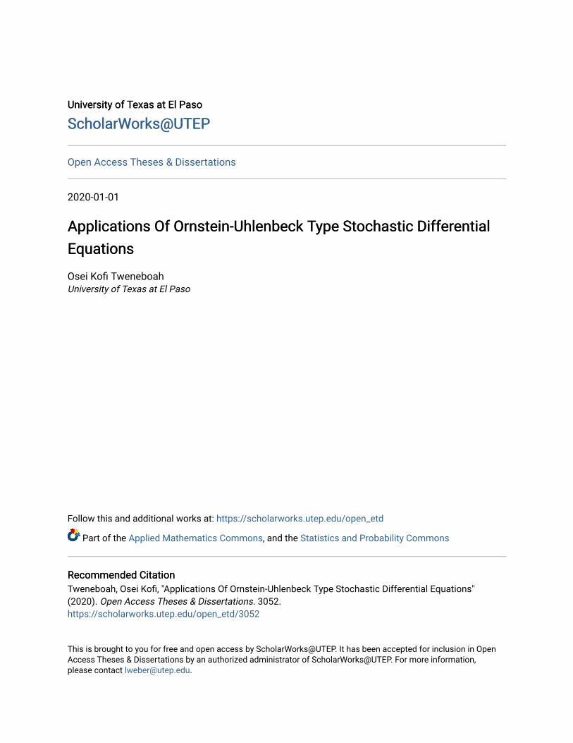
Figure 2.2: Time series data of financial returns from Bank of America (BAC) stock index.

When modeling finite number of random variables, a covariance matrix is usually com-

puted to summarize the dependence between these variables. For a time series Xt∞t=−∞ we

need to model the dependence over infinite number of random variables. The concepts of

autocovariance and autocorrelation functions provide us a tool for this purpose.

Definition 2.2.14 (Autocovariance function). The autocovariance function of a time series Xt with

Var(Xt) < ∞ is defined by

γX(s, t) = Cov(Xs, Xt) = E[(Xs − E[Xs])(Xt − E[Xt])]

With autocovariance functions, we can define the covariance stationarity, or weak station-

arity

Definition 2.2.15 (Stationarity). The time series Xt, t ∈ Z (where Z is the set on integers) is

stationary if

1. E[X2t ] < ∞ for all t ∈ Z.

2. E[Xt] = µ for all t ∈ Z.

3. γX(s, t) = γX(s + h, t + h) for all s, t, h ∈ Z

Based on Definition 2.2.15, we can rewrite the autocovariance function of a stationary pro-

cess as

γX(h) = Cov(Xt, Xt+h) for t, h ∈ Z

17

Definition 2.2.16 (Autocorrelation function). The autocorrelation function of a stationary time series

Xt is defined by

ρX(h) =γX(h)γX(0)

,

where γX(h) = Cov(Xt, Xt+h) and γX(0) = Cov(Xt, Xt).

Remark 2.2.2. When the time series Xt is stationary, we must have

ρX(h) = ρX(−h)

Definition 2.2.17 (Strict Stationary). The time series Xt, t ∈ Z is said to be strict stationary if the

joint distribution of (Xt1 , Xt2 , . . . , Xtk) is the same as (Xt1+h, Xt2+h, . . . , Xtk+h).

Most statistical forecasting methods are based on the assumption that the time series can

be rendered approximately stationary through the use of mathematical transformations. This

is because stationary data series is relatively easy to predict that is, one can simply forecast

that its statistical properties will be the same in the future as they have been in the past. The

predictions for the stationarized series can then be “untransformed,” by reversing whatever

mathematical transformations were previously used, to obtain predictions for the original

series. Non-stationary data on the other hand are unpredictable and cannot be modeled or

forecasted. The results obtained by using non-stationary time series may be false in that they

may indicate a relationship between two variables where actually one does not exist. In order

to receive consistent, reliable results, the non-stationary data needs to be transformed into

stationary data. Examples of non-stationary data includes the population of United States,

income, price changes, and several others.

2.3 Examples of stochastic processes

A Markov process is a simple type of stochastic process in which the time order in a sequence

of events plays a significant role i.e. the present state can influence the probability of what

happens next. We present a formal definition as follows:

18

2.3.1 Markov processes

Definition 2.3.1 (Markov process). The stochastic process Xt is a Markov process if the following

property are satisfied: For every s ∈ T and t ∈ T with s < t, and for every H ∈ Fs and x ∈ S, the

conditional distribution of Xt given H and Xs = x is the same as the conditional distribution of Xt just

given Xs = x:

P(Xt ∈ A|H, Xs = x) = P(Xt ∈ A|Xs = x)

for all A ⊂ S.

The complexity of Markov processes depends greatly on whether the time space or the state

space are discrete or continuous. We will assume that both are discrete, that is we assume that

time space T = N and the state space S is countable. The Brownian motion process and

the Poisson process are both examples of Markov processes [45] in continuous time, whereas

simple random walks on the integers are examples of Markov processes in discrete time [20].

We will discuss the Brownian motion, Poisson process and random walks later in this chapter.

2.3.2 Martingales

Definition 2.3.2 (Martingales). Let (Ω,F , P) be a probability space. A martingale sequence of length

n is a set of variables X1, X2, . . . , Xn and corresponding σ-algebras F1,F2, . . . ,Fn that satisfy the

following relations:

1. Each Xi is an integrable random variable adapted to the corresponding σ-algebra Fi.

2. The Fi’s form a filtration.

3. For every i ∈ [1, 2, . . . , n− 1], we have:

Xi = E [Xi+1|Fi] .

This process has the property that the expected value of the future given the information

we have today is going to be equal to the known value of the process today. In French (a

19

martingale means a winning strategy. This is because for gamblers, a martingale is a bet-

ting strategy where the stake doubled each time the player loses. Players follow this strategy

because, since they will eventually win, they argue they are guaranteed to make money. Ex-

amples of martingales are given below:

1. Let Xt+1 = Xt ± bt where +bt and −bt occur with equal probability bt is measurable Ft,

and the outcome ±bt is measurable Ft+1 (i.e. my “bet” bt can only depend on what has

happened so far and not on the future, but my knowledgeFt includes the outcome of all

past bets). Then Xt|Ft is a martingale.

2. A random ±1 walk is a martingale.

2.3.3 Simple random walk

A random walk is a stochastic sequence Xn, defined by

Xn =n

∑t=1

Xt

where Xt are independent and identically distributed random variables (i.i.d.).

The random walk is simple if Xt = ±1, with P(Xt = 1) = p and P(Xt = −1) = 1− p.

A simple random walk is symmetric if the particle has the same probability for each of the

neighbors. We recall that the simple random walk is both a martingale that is E(Xt+s|Xt) = Xt

and a stationary Markov process that is the distribution of Xt+s|Xt = kt, . . . , X1 = k1 depends

only on the value kt.

2.3.4 The Brownian Motion (Wiener process)

The Brownian motion also called the Wiener process is a continuous-time stochastic process.

Let (Ω,F , P) be a probability space. A Brownian motion is a stochastic process Bt with the

following properties:

1. B0 = 0.

20

2. With probability 1, the function t→ Bt is continuous in t.

3. The process Bt has stationary and independent increments.

4. The increment Bt+s − Bs has a N(0, t) distribution, where N(0, t) denotes the normal

distribution with mean 0 and variance t.

2.4 Levy Processes

Stochastic processes are mathematical models of time evolution of random phenomena. There-

fore the index t is usually taken for time. The most basic process modeled for continuous

random motions is the Brownian motion or Wiener process and that for jumping random mo-

tions is the Poisson process. The Brownian motion was described in the previous section. The

Poisson process will be described in this section.

Before we start our discussion of Levy processes, we present the following definitions.

Definition 2.4.1 (Stochastic Continuity). A stochastic process Xt on Rn is stochastically continu-

ous or continuous in probability if, for every t ≥ 0 and ε > 0,

lims→t

P[|Xs − Xt| > ε] = 0 (2.3)

Definition 2.4.2 (Characteristic Function). The Characteristic Function φ of a random variable X is

the Fourier Stieltjes transform of the distribution function F(x) = P(X ≤ x) :

φX(u) = E[eiuX] =∫ ∞

−∞eiuxdF(x), (2.4)

where i is the imaginary number.

One important property of the characteristic function is the fact that for any random vari-

able X, it always exists, it is continuous, and it determines X univocally. If X and Y are

independent random variables then:

φX+Y(u) = φX(u)φY(u). (2.5)

21

The following are some of the the functions, related to the characteristic function which we

will use in this dissertation:

• The cumulant function: kX(u) = log E[e−uX] = log φ(iu).

• The cumulant characteristic function or characteristic exponent:

ψX(u) = log E[eiuX] = log φ(u),

or equivalently

φX(u) = eψ(u). (2.6)

Definition 2.4.3 (Infinitely Divisible Distribution, [50]). Suppose φ(u) is the characteristic function

of a random variable X. If for every positive integer n, φ(u) is also the nth power of a characteristic

function, we say that the distribution is infinitely divisible. Equivalently, in terms of X for any n:

X = Y(n)1 + . . . + Y(n)

n

where Y(n)i , i = 1, . . . n, are independently and identically distributed random variables, all following a

law with characteristic function φ(z)1n .

We begin this section with the definition of a Levy Process.

Definition 2.4.4 (Levy Process). A stochastic process Xt : t ≥ 0 on Rn is a Levy process if the

following conditions are satisfied.

1. For any choice of n ≥ 1 and 0 ≤ t0 < t1 < · · · < tn, random variables Xt0 , Xt1 − Xt0 , Xt2 −

Xt1 , . . . , Xtn − Xtn−1 are independent. That is, the process has independent increments.

2. X0 = 0.

3. The distribution of Xs+t−Xs does not depend on s. That is, the process has stationary increments.

4. It is stochastically continuous.

22

5. There is Ω0 ∈ F with P[Ω0] = 1 such that, for every ω ∈ Ω0, Xt(ω) is right-continuous in

t ≥ 0 and has left limits in t > 0.

A Levy process on Rn is called an n-dimensional Levy process. The law at time t of a

Levy process is completely determined by the law of X1. The only degree of freedom we

have in specifying a Levy process is to define its distribution at a single time. The following

theorem describes the one-to-one relationship between Levy processes and infinitely divisible

distributions.

Theorem 2.4.1 (Infinite Divisibility of Levy Processes). Let X = Xt, t ≥ 0 be a Levy process.

Then X = Xt, t ≥ 0 has infinitely divisible distributions F for every t. Conversely if F is an infinitely

divisible distribution there exists a Levy Process X = Xt, t ≥ 0 such that the distribution of X1 is

given by F.

We can further write

φXt(u) = E[e−iuXt ] = etψ(u)

where ψX(u) = log(φ(u)) is the characteristic exponent as in (3.25). The characteristic expo-

nent ψ(u) of a Levy Process satisfies the following Levy- Khintchine formula ([47]):

ψ(u) = iγu− 12

σ2u2 +∫ ∞

−∞(eiux − 1− iuxI|x|<1)ν(dx), (2.7)

where γ ∈ R, σ2 ≥ 0 and ν is a measure on R\0 with∫ ∞

−∞inf1, x2ν(dx) =

∫ ∞

−∞(1∧ x2)ν(dx) < ∞. (2.8)

From (2.7), we observe that, generally a Levy process consist of 3 independent parts namely: a

linear deterministic part, a Brownian part, and a pure jump part. We say that the correspond-

ing infinitely divisible distribution has a Levy triplet [γ, σ2, ν(dx)]. The measure ν is called the

Levy measure of X.

Definition 2.4.5 (Levy measure). Let Xt : t ≥ 0 be a Levy Process on Rn. The measure ν on Rn

defined by;

ν(A) =1t

E

(∑

0<s≤tI∆Xs∈A

), A ∈ B(R) (2.9)

23

is called a Levy measure. The measure ν(A) dictates how jumps occur. In particular jumps of sizes in

the set A occur according to a Poisson process with parameter ν(A) =∫

A ν(dx). In other words, ν(A)

is the expected number of jumps per unit time, whose size belongs to A.

A Levy measure has no mass at the origin, but singularities that is infinitely many jumps

can occur near the origin (small jumps). Special attention has to be considered on small

jumps. The sum of all jumps smaller than some ε > 0 may not converge. For instance,

consider the example where the Levy measure ν(dx) = dxx2 , as we move closer to the origin

there is an increasingly large number of small jumps and∫ 1−1 |x|ν(dx) = +∞. But the integral∫ 1

−1 x2ν(dx) =∫ 1−1 x2 dx

x2 =∫ 1−1 dx is still finite. However, as we move away from the origin,

ν([−1, 1]c) is finite and we do not experience any difficulties with the integral in (2.8) being

finite. Brownian motion has continuous sample paths with no jumps and as such ∆Xt = 0.

On the hand, Poisson process with rate parameter a and jump sizes equal to 1 is a pure jump

process with ∆Xt = 1 and Levy measure ν(A) =

a if 1 ∈ A

0 if 1 /∈ AIf the Levy measure is of the form ν(dx) = u(x)dx, then u(x) is known as the Levy density.

The Levy density has properties similar to a probability density, however, it need not be

integrable and must have zero mass at the origin.

2.4.1 Properties of Levy Processes

If σ2 = 0 and∫ +1−1 |x|ν(dx) < ∞, it follows from standard Levy process theory that the process

is of finite variation see [48], [47]. Moreover, there is a finite number of jumps in any finite

interval and the process is said to be of finite activity.

The Brownian motion is of infinite variation, therefore a Levy process with a Brownian

component is of infinite variation. A pure jump Levy process is of infinite variation if and

only if∫ +1−1 |x|ν(dx) = ∞. In this instance, special attention has to paid to the small jumps.

Basically, the sum of all jumps smaller than ε > 0 does not converge. However, the sum of the

24

jumps compensated by their mean does not converge. This peculiarity leads to the necessity

of the compensator term iuxI|x|<1 in (2.7).

2.5 Examples of Levy Processes

In this section we give examples of some popular Levy processes and describe the main prop-

erties, which we will use in this dissertation systematically. We will start with subordinators.

Next, we will present some examples of Levy processes that live on the real line. Much at-

tention will be paid to their density function, their characteristic function, their Levy triplets

and some important properties. We compute moments, variance, skewness and kurtosis, if

possible. For more examples of Levy processes, see [49], [50] and [2].

2.5.1 Poisson Process

Definition 2.5.1 (Poisson Process). A stochastic process N = Nt, t ≥ 0 with intensity parameter

λ > 0 is a Poisson process if it fulfills the following conditions:

1. N0 = 0.

2. The process has independent increments.

3. The process has stationary increments.

4. For s < t the random variable Nt − Ns has a Poisson distribution with parameter λ(t− s):

P[Nt − Ns = n] =λn(t− s)n

n!e−λ(t−s)

.

The Poisson process is the simplest of all the Levy processes. It is based on the Poisson

distribution, which depends on the parameter λ > 0 and has the the following characteristic

function:

φPoisson(u; λ) = exp(λ(exp(iu)− 1)).

25

The Poisson distribution lives on the non-negative integers k = 0, 1, 2, . . . and the probability

mass function at point k is given by:

f (k; λ) =λke−λ

k!.

Since the Poisson distribution is infinitely divisible, we can define a Poisson process N =

Nt, t ≥ 0with intensity parameter λ > 0 as the process which starts at zero, has independent

and stationary increments and where the increments over a time interval of length s > 0

follows the Poisson(λs) distribution. The Poisson process is an increasing pure jump process,

with jump sizes equal to 1. The time between two consecutive jumps follows an exponential

distribution with mean λ−1, that is a Γ(1, λ) law. The moments of the Poisson distribution are

given in Table 2.2.

Table 2.2: Moments of the Poisson distribution with intensity λ

Poisson(λ)

Mean λ

Variance λ

Skewness 1√λ

Kurtosis 3 + λ−1

2.5.2 Compound Poisson Process

Definition 2.5.2 (Compound Poisson Process). A compound Poisson process with intensity param-

eter λ and a jumps size distribution L is a stochastic process Z = Zt, t ≥ 0 defined as:

Zt =Nt

∑k=1

χk (2.10)

where N = Nt, t ≥ 0 is a Poisson process with intensity parameter λ and (χk, k = 1, 2, . . . ) is an

independently and identically distributed sequence.

26

The sample paths of Z = Zt, t ≥ 0 are piecewise constant and the value of the process at

time t, Zt, is the sum of Nt random numbers with law L. The jump times have the same law

as those of the Poisson process N = Nt, t ≥ 0. The ordinary Poisson process corresponds to

the case where χk = 1, k = 1, 2, . . . . The characteristic function of Zt is given by

E[exp(iuZt)] = exp(

t∫ ∞

−∞(exp(iux)− 1)ν(dx)

)∀u ∈ R, (2.11)

where ν is called the Levy measure of process Z = Zt, t ≥ 0. ν is a positive measure on R but

not a probability measure since∫

ν(dx) = λ 6= 1.

2.5.3 The Gamma Process

Definition 2.5.3 (Gamma Process). A stochastic process X = Xt, t ≥ 0 with parameters a and b

is a Gamma process if it fulfills the following conditions:

1. X0 = 0.

2. The process has independent increments.

3. The process has stationary increments.

4. For s < t the random variable Xt − Xs has a Gamma(a(t− s), b) distribution.

A random variable X has a Gamma distribution Γ(a, b) with rate and shape parameters

a > 0 and b > 0 respectively, if its density function is given by:

fX(x; a, b) =ba

Γ(a)xa−1e−bx, ∀x > 0. (2.12)

The moments of the Γ(a, b) distribution are given in Table 2.3.

.

The Gamma process is a non-decreasing Levy process and its characteristic function is

given by:

φ(u; a, b) = (1− iub)−a. (2.13)

27

Table 2.3: Moments of the Γ(a, b) distribution

Γ(a, b)

Mean ab

Variance ab2

Skewness 2a12

Kurtosis 3(1 + 2a−1)

2.5.4 Inverse Gaussian Process

Let T(a,b) be the first time a standard Brownian motion with drift b > 0, that is Ws + bs, s ≥ 0,

reaches a positive level a > 0. The random time follows the inverse Gaussian, IG(a, b), law

and has a characteristic function:

φ(u; a, b) = exp(−a(√−2iu + b2 − b)).

The inverse Gaussian distribution is infinitely divisible and we define the inverse Gaussian

process X = Xt, t ≥ 0, with parameters a, b > 0, as the process which starts at zero and has

independent and stationary increments such that

E[exp(iuXt)] = φ(u; at, b)

= exp(−at(√−2iu + b2 − b)).

(2.14)

2.6 Subordination of Levy processes

Subordination is a transformation of a stochastic process to a new stochastic process through

a random time change by increasing Levy process (subordinator) independent of the original

process. The new process is called a subordinate to the original one. The idea of subordination

was introduced by Bochner [12] in 1949.

Definition 2.6.1 (Subordinator). A subordinator is a one-dimensional Levy process that is non-

decreasing almost surely. Such processes can be thought of as a random model of time evolution,

28

since if T = (T(t), t ≥ 0) is a subordinator we have,

T(t) ≥ 0 a.s for each t > 0,

and

T(t1) ≤ T(t2) a.s whenever t1 ≤ t2.

Theorem 2.6.1. If T is a subordinator, then its Levy symbol takes the form

η(u) = ibu +∫ ∞

0(eiuy − 1)λ(dy), (2.15)

where b ≥ 0 and the Levy measure λ satisfies the additional requirements

λ(−∞, 0) = 0 and∫ ∞

0(y ∧ 1)λ(dy) < ∞.

Conversely, any mapping from Rd → C of the form (2.15) is the Levy symbol of a subordinator.

The proof of Theorem 2.6.1 can be found in [47]. The pair (b, λ) is the characteristic of the

subordinator T.

Some classical examples of a subordinators are the Poisson process, compound Poisson

process (if and only if the (χk, k = 1, 2, . . . ) in (2.10) are all R+− valued), Gamma process and

many others. For more examples of subordinators, see Ref. [2].

We begin the second part of this chapter which is dedicated to the discussion of stochastic

differential equation. We start our discussion with the concept of deterministic differential

equations.

2.7 Deterministic Differential Equations

The theory of differential equations is the provenience of classical calculus and it motivated the

creation of differential and integral calculus. A differential equation is an equation involving

29

an unknown function and its derivative. The idea underlying a differential is simple. Given a

functional relationship

f (t, x(t), x′(t), x′′(t), . . . ) = 0, 0 ≤ t ≤ T (2.16)

involving the time t, an unknown function x(t) and its derivative. The solution of the differ-

ential equation (2.16) is to find a function x(t) which satisfies (2.16).

The simplest differential equations are those of order 1. They involve only t, x(t) and

the first derivative x′(t). The standard form for the first-order differential equation in the

unknown function x(t) is

x′(t) =dx(t)

dt= a(t, x(t)), x(0) = x0, (2.17)

where a(x, t) is a known function and the derivative x′(t) appears only on the left side of

(2.17).

Example 2.7.1 (Exponential growth model). Consider the simple population growth model

dNdt

= k(t)N(t), N(0) = N0 (2.18)

where N(t) is the size of the population at time t, and k(t) is the relative rate of growth at time t.

Integration on both sides yields the solution∫ dNN(t)

=∫

k(t)dt =⇒ N(t) = N0e∫

k(t)dt

Example 2.7.2 (Separation of variables). Suppose the right-hand side of (2.17) can be separated into

a product of two functions:

x′(t) =dxdt

= a1(t)a2(x(t)). (2.19)

Equation (2.19) can be rewritten asdx

a2(x(t))= a1(t). (2.20)

Integration on both sides yields the solution∫ x(t)

x(0)

dxa2(t)

=∫ t

0a(s)ds. (2.21)

30

On the left-hand side we obtain a function x(t), on the right-hand side a function of t.

Thus, we have obtain an explicit form of the function x(t).

Remark 2.7.1. Integrating both sides of (2.17) , one obtains an equivalent integral equation:

x(t) = x(0) +∫ t

0a(s, x(s))ds. (2.22)

The transformed equation is generally not used to find the solution of (2.19). It however gives an idea

of how we could define a stochastic integral equation.

In the exponential growth model in Example 2.7.1, it might happen that k(t) is not com-

pletely known, but subject to some random environmental effects i.e.

k(t) = b(t) + “noise”

where we do not know the exact behavior of the noise term, only its probability distribu-

tion. The function b(t) is assumed to be nonrandom.

2.8 Ito Integrals

We begin this section by finding a mathematical interpretation of the “noise” term in the

equation of Example 2.7.1. We recall that,

dNdt

= (b(t) + “noise” )N(t) (2.23)

More generally, we can rewrite the above in the form

dXdt

= b(t, Xt) + σ(t, Xt) · “noise” (2.24)

where b(t, Xt) and σ(t, Xt) are some given deterministic functions. If we consider the case

where the noise is 1-dimensional, we can describe the noise term by some stochastic process

Wt, so that

31

dXdt

= b(t, Xt) + σ(t, Xt) ·Wt (2.25)

The stochastic process Wt has the following properties:

(i) For t1 6= t2 implies that the stochastic processes Wt1 and Wt2 are independent.

(ii) The stochastic process Wt is stationary, i.e. the joint distribution of Wt1+t, . . . , Wtk+t

does not depend on t.

(iii) E[Wt] = 0 for all t.

It turns out that there does not exist any suitable stochastic process satisfying properties

(i) and (ii) i.e. such a Wt cannot have a continuous paths. However we can represent Wt as a

generalized stochastic process called the white noise process. Here generalized means that the

process can be constructed as a probability measure on the space of tempered distributions on

[0, ∞), and not as a probability measure on the much smaller space R[0,∞).

If we let 0 = t0 < t1 < . . . < tm = t we can discritize (2.25) as follows:

Xk+1 − Xk = b(tk, Xk)∆tk + σ(tk, Xk)Wk∆tk (2.26)

where Xj = X(tj), Wk = Wtk and ∆tk = tk+1 − tk

Replacing Wk∆tk by ∆Vk = Vtk+1 − Vtk in (2.26) where Vtt≥0 is a suitable stochastic

process. The properties (i), (ii) and (iii) on Wt suggest that Vt should be stationary. The only

process with continuous paths is the Brownian motion Bt. Therefore we substitute Vt with Bt

in eqrefexample-population-ito2 to obtain:

Xk = X0 +k−1

∑j=0

b(tj, Xj)δtj +k−1

∑j=0

σ(tj, Xj)∆Bj (2.27)

Assuming that the limit of the right hand side of (2.27) exist when ∆tj → 0, then applying

the usual integration notation we obtain

Xt = X0 +∫

b(s, Xs)ds +∫

σ(s, Xs)dBs (2.28)

32

where the first integral on the right-hand side is a Riemann integral, and the second one

is an Ito stochastic integral. We would adopt as a convention that (2.27) really means that

Xt = Xt(ω) is a stochastic process satisfying (2.28).

We will proceed to prove the existence of∫ t

0f (s, ω)dBs(ω), (2.29)

where Bt(ω) is a 1- dimensional Brownian motion starting at the origin, for a wide class of

functions f : [0, ∞]×Ω→ R.

Definition 2.8.1 (The Ito integral). Let f ∈ V(S, T). Then the Ito integral of f is defined by∫ T

sf (t, ω)dBt(ω) = lim

x→∞

∫ T

sφn(t, ω)dBt(ω), (2.30)

where φn is a sequence of elementary functions such that

E

[∫ T

s( f (t, ω)− φn(t, ω))2dt

]→ 0 as n→ ∞. (2.31)

From Definition 2.8.1, we get the following,

Corollary 2.8.1 (The Ito Isometry).

E

[(∫ T

sf (t, ω)dBt

)2]= E

[(∫ T

sf 2(t, ω)dt

)]∀ f ∈ V(S, T). (2.32)

Corollary 2.8.2 (The Ito Isometry). If f (t, ω) ∈ V(S, T) and fn(t, ω) ∈ V(S, T) for n = 1, 2, . . .

and E[∫ T

s fn(t, ω)− f (t, ω)dt]→ 0 as n→ ∞, then

∫ T

sfn(t, ω)dBt(w)→

∫ T

sf (t, ω)dBt(w) in L2(P) as n→ ∞. (2.33)

Theorem 2.8.1 (Integration by parts). Suppose f (s, ω) = f (s) only depends on s and that f is

continuous and of bounded variation in [0, t]. Then∫ t

0f (s)dBs = f (t)Bt −

∫ t

0Bsd fs. (2.34)

33

2.8.1 Properties of the Ito integral

Theorem 2.8.2. Let f , g ∈ V(S, T) and let 0 ≤ S < U < T. Then

1.∫ T

S f dBt =∫ U

S f dBt +∫ T

U f dBt.

2.∫ T

S (c f + g)dBt = c∫ T

S f dBt +∫ T

S gdBt, for c ∈ R.

3. E[(∫ T

S f dBt

)]= 0.

4.∫ T

S f dBt is FT− measurable.

Another important property of the Ito integral is the fact that it is a martingale.

Definition 2.8.2. A filtration on (Ω,F ) is a familyM = Mtt≥0 of σ algebrasMt ⊂ F such that

0 ≤ s < t =⇒ Ms ⊂Mt.

An n− dimensional stochastic process Mtt≥0 on (Ω,F , P) is called a martingale with respect to a

filtration Mtt≥0 if

(i) Mt isMt− measurable for all t.

(ii) E [|Mt| < ∞] for all t.

(iii) E [Ms|Mt] =Mt for all s ≥ t.

The expectation in (ii) and the conditional expectation in (iii) is taken with respect to

P = P0.

Example 2.8.1. Brownian motion Bt in Rn is a martingale with respect to the σ− algebras Ft generated

by Bs; s ≤ t, because

E[|Bt|]2 ≤ E[|Bt|2] = |B0|2 + nt and if s ≥ t then

E[Bs|Ft] = E[Bs − Bt + Bt|Ft]

= E[Bs − Bt|Ft] + E[Bt|Ft]

= 0 + Bt.

From Example 2.8.1, Ito integrals are martingales. Thus Ito integral gives an important

computational advantage, even though it does not behave so nicely under transformations.

34

2.9 Ito Lemma

In the last section we discussed the Ito stochastic integral. The integral∫ T

s f (t, ω)dBt is now

known to be defined, however we do not know the tools to calculate Ito stochastic integrals.

The objective of this section is to provide such a too, the Ito lemma. The Ito lemma is a very

useful tool for evaluating Ito integrals. For example∫ t

0BsdBs =

12

B2t −

12

t or12

B2t =

12

t +∫ t

0BsdBs (2.35)

The image of the Ito integral Bt =∫ t

0 dBs by the map g(x) = 12 x2 is not again an Ito integral of

the form ∫ t

0f (s, ω)dBs(ω)

but a combination of a dBs− and a ds− integral:

12

B2t =

12

t +∫ t

0BsdBs. (2.36)

It turns out that if we introduce Ito stochastic integrals as sums of dBs− and ds− a integral

then this family of integrals is stable under smooth maps.

Definition 2.9.1 (1− dimensional Ito Stochastic Integral ). Let Bt be a 1− dimensional Brownian

motion on (Ω,F , P). A 1− Ito stochastic integral is a stochastic process Xt on (Ω,F , P) which is of

the form of

Xt = X0 +∫ t

0a(s, ω)ds +

∫ t

0b(s, ω)dBs, 0 ≤ t ≤ T, (2.37)

so that

P

[∫ t

0b(s, ω)2ds < ∞ ∀ t ≥ 0

]= 1 (2.38)

and

P

[∫ t

0|a(s, ω)|ds < ∞ ∀ t ≥ 0

]= 1 (2.39)

If Xt is an Ito stochastic integral of the form of =(2.37) then (2.37) in its differential form is

dXt = adt + bdBt, X0(ω) = Y(ω). (2.40)

35

B = (Bt, t ≥ 0) denotes Brownian motion, and a and b are deterministic functions.

Theorem 2.9.1 (The 1− dimensional Ito lemma). Let Xt be an Ito stochastic differential equation

given by

dXt = adt + bdBt, X0(ω) = Y(ω). (2.41)

Let g(t, x) ∈ C2([0, ∞)×R), that is g is twice continuously differentiable on [0, ∞)×R. Then

Yt = g(t, Xt)

is also an Ito stochastic differential equation, and

dYt =∂g(t, Xt)

∂tdt +

∂g(t, Xt)

∂xdXt +

12

∂2g(t, Xt)

∂x2 · (dXt)2, (2.42)

where (dXt)2 = (dXt) · (dXt) is computed according to the rules

dt · dt = dt · dBt = dBt · dt = 0, dBt · dBt = dt. (2.43)

Proof. Assume that g, ∂g∂t , ∂g

∂x and ∂2g∂x2 are bounded and assume that a(t, ω) and b(t, ω) are ele-

mentary functions. Using Taylor’s theorem we get

g(t, Xt) = g(0, X0) + ∑j

∆g(ti, Xj) = g(0, X0) + ∑j

∂g∂t

∆tj + ∑j

∂g∂x

∆Xj

+12 ∑

j

∂2g∂t2 (∆tj)

2 + ∑j

∂2g∂t∂x

(∆tj)(∆Xj) +12 ∑

j

∂2g∂x2 (∆Xj)

2 + ∑j

Rj

(2.44)

where ∂g∂t , ∂g

∂x etc. are evaluated at the points (tj, Xtj), ∆tj = tj+1 − tj, ∆Xj = Xtj+1 − Xtj ,

∆g(tj, Xj) = g(tj+1, Xtj+1)− g(tj, Xj) and Rj = O(|∆tj|2 + |∆Xj|2) ∀ j.

If ∆tj → 0 then

∑j

∂g∂t

∆tj = ∑j

∂g∂t

(tj, Xj)∆tj →∫ t

0

∂g∂t

(s, Xs)ds (2.45)

∑j

∂g∂x

∆tj = ∑j

∂g∂t

(tj, Xj)∆Xj →∫ t

0

∂g∂t

(s, Xs)dXs. (2.46)

Moreover, since a and b are elementary functions, we get

36

∑j

∂2g∂x2 (∆Xj)

2 = ∑j

∂2g∂x2 a2

j (∆tj)2 + ∑

j

∂2g∂x2 ajbj(∆tj)(∆Bj)

+ ∑j

∂2g∂x2 bj(∆Bj)

2,(2.47)

where aj = a(tj, ω) and bj = b(tj, ω).

The first two terms in (2.47) tend to 0 as ∆tj → 0. For example

E

(∑j

∂2g∂x2 ajbj(∆tj)(∆Bj)

)2 = ∑

jE

(∑j

∂2g∂x2 ajbj

)2 (∆tj)

3 → 0 as ∆tj → 0.

Claim:

The last term in (2.47) tends to∫ t

0

∂2g∂x2 b2ds in L2(P), as ∆tj → 0.

To prove this claim, put u(t) = ∂2g∂x2 (t, Xt)b2(t, ω), uj = u(tj) and consider

E

(∑j

uj(∆Bj)2 −∑

juj∆tj

)2 = ∑

i,jE[uiuj((∆Bi)

2 − ∆ti)((∆Bj)2 − ∆tj)].

If i < j then uiuj((∆Bi)2 − ∆ti) and (∆Bj)

2 − ∆tj are independent so the terms vanish in this

case, and similarly if i > j. So we are left with

∑j

E[u2j ((∆Bj)

2 − ∆tj)2] = ∑

jE[u2

j ] ·E[(∆Bj)4 − (∆Bj)

2∆tj + (∆tj)2]

= ∑j

E[u2j ] · (3(∆tj)

2 − 2(∆tj)2 + (∆tj)

2)

= 2 ∑j

E[u2j ] · (∆tj)

2 → 0 as ∆tj → 0.

Thus we have established that

∑j(∆Bj)

2 →∫ t

0u(s)ds in L2(P) as ∆tj → 0

37

and this is often expressed by the formula

(dBt)2 = dt. (2.48)

The argument above also proves that ∑j Rj → 0 as ∆tj → 0. This completes the proof of

the Ito lemma.

Remark 2.9.1. It is enough that g(t, x) is C2 on [0, ∞) × U, if U ⊂ R is an open set such that

Xt(ω) ∈ U for all t ≥ 0, ω ∈ Ω. Moreover, it is sufficient that g(t, x) is C1 with respect to t and C2

with respect to x.

Next we present the general Ito formula.

Theorem 2.9.2 (The general Ito formula). Suppose Bt = (B1(t), . . . , Bd(t)) is a d-dimensional

Brownian motion. Recall that each component is a standard Brownian motion.

Let X = (X1(t), X2(t), . . . , Xd(t)), be an n-dimensional Ito process, that is,

dXi(t) = µidt + σi1dB1(t) + σi2dB2(t) + · · ·+ σiddBd(t) (2.49)

for all i from 1 to n. Equation (2.49) can be represented in matrix form as

dXt = Udt + ΣdBt,

where

U =

µ1

µ2...

µn

, and Σ =

σ11 σ12 . . . σ1d

σ21 σ22 . . . σ2d...

... . . . ...

σn1 σn2 . . . σnd

Suppose that f (t, x) = ( f1(t, x), f2(t, x), . . . , fm(t, x)) is a function defined on [0, ∞)×Rn with

values in Rm with f ∈ C1,2 ([0, ∞)×Rn).

Then, the process Yt = f (t, Xt) is also an Ito process and its component k is given by

dYk(t) =∂ fk∂t

dt +n

∑i=1

∂ fk∂xi

dXi(t) +12

n

∑i,j=1

∂2 fk∂xi∂xj

(dXi(t))(dXj(t)),

38

for all k from 1 to m. The last term is calculated using the following rules:

dtdt = dBi(t)dt = dtdBi(t) = dBi(t)dBj(t) = 0, ∀i 6= j

dBi(t)dBi(t) = dt.

The proof of the above theorem follows from the proof of Theorem 2.9.1.

2.10 One-dimensional Stochastic Differential Equation

A one-dimensional stochastic differential equation can be understood as a deterministic dif-

ferential equation which is perturbed by random noise.

We recall the stochastic differential equation (2.25) defined in Section 2.8 of this chapter:

dXdt

= b(t, Xt) + σ(t, Xt)Wt (2.50)

where b(t, x) and σ(t, x) are both in R and Wt is a 1-dimensional “white noise”. As mentioned

earlier in Section 2.8, the Ito interpretation of (2.50) is that Xt satisfies the stochastic integral

equation

Xt = X0 +∫ t

0b(s, Xs)ds +

∫ t

0σ(s, Xs)dBs (2.51)

or in differential form

dXt = b(t, Xt)dt + σ(t, Xt)dBt (2.52)

We obtained dBt in (2.52) by replacing the white noise in (2.50) with dBtdt and then multiply by

dt.

Given a stochastic differential equation, two question that normally arises are

1. Can one obtain existence and uniqueness theorems for such equations? What are the

properties of the solutions?

39

2. How can one solve such equations?

We now discuss the existence and uniqueness question 1 above.

2.10.1 An Existence and Uniqueness Result

Theorem 2.10.1 (Existence and Uniqueness theorem for stochastic differential equations). Let

T > 0 and a(·, ·) : [0, T]×Rn → Rn, b(·, ·) : [0, T]×Rn → Rn×m be measurable functions satisfying

|b(t, x)|+ |σ(t, x)| ≤ C(1 + |x|); x ∈ Rn, t ∈ [0, T] (2.53)

for some constant C, (where |σ|2 = ∑ |σij|2) and such that

|b(t, x)− b(t, y)|+ |σ(t, x)− σ(t, y)| ≤ D|x− y|; x, y ∈ Rn, t ∈ [0, T] (2.54)

for some constant D. Let Z be a random variable which is independent of the σ− algebra F (m)∞ generated

by Bs(·), s ≥ 0 and such that

E[|Z|2] < ∞.

Then the stochastic differential equation

dXt = b(t, Xt)dt + σ(t, Xt)dBt, 0 ≤ t ≤ T, X0 = Z (2.55)

has a unique t− continuous solution Xt(ω) with the property that Xt(ω) is adapted to the filtration

FZt generated by Z and

Bs(·); s ≤ t and (2.56)

E

[∫ T

0|Xt|2dt

]< ∞. (2.57)

Conditions (2.53) and (2.54) are natural in view of the following two simple examples from

deterministic equations i.e. σ = 0.

Example 2.10.1. 1. The equationdXt

dt= X2

t , X0 = 1 (2.58)

40

corresponding to b(x) = x2 (which does not satisfy condition (2.53) has the (unique) solution

Xt =1

1− t; 0 ≤ t < 1.

Thus it is impossible to find a global solution (defined for all t) in this case. More generally,

condition (2.53) ensures that the solution Xt(ω) of (2.55) does not explode, that is, |Xt(ω)| does

not tend to ∞ in a finite time.

2. The equationdXt

dt= 3X2/3

t ; X0 = 0 (2.59)

has more than one solution. In fact, for any u > 0 the function

Xt =

0 for t ≤ a

(t− u)3 for t > a

solves (2.59). In this case b(x) = 3x2/3 does not satisfy the Lipschitz condition (2.54) at x = 0.

Thus condition (2.54) guarantees that (2.55) has a unique solution. Here uniqueness means that

if X1(t, ω) and X2(t, ω) are two t− continuous processes satisfying equations (2.55), (2.56) and

(2.57) then

X1(t, ω) = X2(t, ω) for all t ≤ T, a.s. (2.60)

For the second question, the Ito lemma is the used as a solution method to many stochastic

differential equations.

2.10.2 Weak and Strong Solutions

Definition 2.10.1 (Strong Solution). A strong solution to the Ito stochastic differential equation (2.37)

is a stochastic process Xt = (Xt, t ∈ [0, T]) which satisfies the following conditions:

• Xt is adapted to the Brownian motion, that is, at time t it is a function of Bs, s ≤ t.

• The integrals occurring in (2.37) are well defined as Riemann and Ito stochastic integrals respec-

tively.

41

• Xt is a function of the underlying Brownian sample path and of the coefficient functions b(t, x)

and σ(t, x). Thus a strong solution to (2.37) is based on the path of the underlying Brownian

motion.

Equivalently, a solution Xt to a stochastic differential Equation is called a strong solution if the version

of Bt of Brownian motion is given in advance and the solution Xt constructed from it is FZt − adapted.

Definition 2.10.2 (Weak Solution). A solution Xt to a stochastic differential Equation is called a

weak solution if we are only given the functions b(t, x) and σ(t, x) and ask for a pair of processes

((Xt, Bt), Ht) on a probability space (Ω,H, P) such that condition (2.54) holds. Ht is an increasing

family of σ−algebras such that Xt is Ht− adapted and Bt is an Ht− Brownian motion, that is Bt is a

Brownian motion, and Bt is a a martingale with respect to Ht.

For these solutions, the path behavior is is not essential, we are only interested in the distribution Xt.

Weak solutions Xt are sufficient in order to determine the distributional characteristics of Xt such as

the expectation, variance and covariance functions of the process.

Remark 2.10.1. A strong solution is of course also a weak solution, but the converse is not true in

general.

2.11 Multi-dimensional Stochastic Differential Equations

If a finite number of SDEs are given in a model, then the multi-dimensional case should be

considered. This situation can arise for the modeling of several phenomena, e.g., the price

evolution of multiple stocks, interest rates, volatilities and several others see [43], [28].

For the case of random fluctuation in higher dimensions (i.e. m ≥ 2), let Bt = (B1t , B2

t , . . . , Bmt )

T

denote m− dimensional Brownian motion at time t. In this case, the deterministic (drift)

part b : Rd ×R+ → Rd, namely, b(Xt, t) is a measurable vector process the diffusion part

σ : Rd ×R+ → Rd×m, namely, œ(Xt, t) is a measurable matrix-valued process.

For the underlying probability space (Ω, F, P), adapted to the filtration (F)t≥0, a d− di-

mensional stochastic process X = (Xt : t ∈ [0, ∞)) is represented by d differential equations,

42

d− dimensional initial vector and suitable conditions.

If we write a coupled system of SDEs with d processes of states and m− dimensional

Brownian motions, we obtain:

dXt = b(Xt, t)dt + σ(Xt, t)dBt (2.61)

where

Xt =

X1(t)

X2(t)...

Xd(t)

, b(Xt, t) =

b1(Xt, t)

b2(Xt, t)...

bd(Xt, t)

, dBt =

dB1(t)

dB2(t)...

dBm(t)

σ(Xt, t) =

σ11(Xt, t) σ12(Xt, t) . . . σ1m(Xt, t)

σ21(Xt, t) σ22(Xt, t) . . . σ2m(Xt, t)...

... . . . ...

σd1(Xt, t) σd2(Xt, t) . . . σdm(Xt, t)

,

For comprehensive study of the stochastic differential equation and its solution methods,

see [40], [43], [28] and references therein.

2.12 Simulation of stochastic differential equations

In this section we will discuss the simulation of SDEs focusing mainly on the Euler–Maruyama

method [38] and Euler–Milstein scheme [41] for approximating the sample path of SDE’s.

Please refer to [22] for other techniques used to generate sample paths of SDEs. We begin our

discussion with the Euler–Maruyama method which is also known as the Euler method.

43

2.12.1 Euler–Maruyama scheme for approximating stochastic differential

equations

The Euler–Maruyama method is a technique used to approximate the numerical solution of a

stochastic differential equation. It is a generalization of the Euler method for approximating

ordinary differential equations to stochastic differential equations. Consider the following

SDE:

dXt = b(t, Xt)dt + σ(t, Xt)dBt, (2.62)

with initial condition X0 = x0 and Bt a 1-dimensional standard Brownian motion. The solution

of (2.62) is given as:

Xt = x0 +∫ t

0b(s, Xs)ds +

∫ t

0σ(s, Xs)dBs. (2.63)

Therefore, approximating the path of Xt is equivalent to approximating the integral. There

are several ways to approximate the first integral, the second however has to be approximated

using the Euler scheme. The Euler method uses a simple rectangular rule. First assume

that the interval [0, t] is divided into n equal subintervals. This implies that the increment is

∆t = t/n and that the points are t0 = 0, t1 = ∆t, . . . , ti = i∆t, . . . , tn = n∆t = t. Thus using Xi

to denote Xti we have:X0 = x0

Xi = Xi−1 + b(ti−1, Xi−1)∆t + σ(ti−1, Xi−1)∆Bi, ∀i ∈ 1, 2, . . . , n,

where ∆Bi is the increment of a standard Brownian motion over the interval [ti−1, ti]. We recall

that the Brownian motion has independent and stationary increments, so it follows that each of

such increment is independent of all others and is distributed as a normal (Gaussian) random

variable with mean 0 and variance the length of the time sub-interval (i.e. ∆t). Therefore, the

standard deviation of the increment is√

∆t.

The Euler–Maruyama algorithm for generating the sample paths of example 2.63 using a

fixed number of paths, n, and discretization interval, ∆t are presented in Algorithm 1.

44

Algorithm 1 Generating a sample path using Euler–Maruyama’s method to estimate θ =

E[ f (Xt)].

for j = 1 to n do

t = 0; X = X0

for k = 1 to [T/∆t] =: m do

generate Z ∼ N(0, 1)

set X = X + b(t, X)∆t + σ(t, X)√

∆tZ

set t = t + ∆t

end for

set f j = f (X)

end for

set θn = ( f1 + . . . + fn)/n

set σ2n = ∑n

j=1( f j − θn)2/(n− 1)

set approximately 100(1− α)% CI = θn ± z1−α/2σn√

n

45

This algorithm can be extended to general b and σ functions by creating separate functions.

The scheme can also be generalized to approximate multidimensional SDEs. In the multidi-

mensional case, Xt ∈ Rd, Bt ∈ Rp and b(t, Xt) ∈ R are vectors and σ(t, Xt) ∈ Rd×p is a matrix.

The Euler–Maruyama method gives a first-order approximation for the stochastic integral.

The Euler–Milstein method discussed in the next subsection provides an improvement by

including second-order terms.

2.12.2 Euler–Milstein scheme for approximating stochastic differential equa-

tions

The Euler–Milstein scheme is a technique for approximating the numerical solution of a

stochastic differential equation. The idea in this scheme is to consider expansions on the

coefficients b and σ. This method is applied when the coefficients of the process are functions

of only the main process i.e. do not depend on time. The scheme is designed to work with

SDEs of the type

dXt = b(Xt)dt + σ(Xt)dBt,

with initial conditions X0 = x0. We consider expansions on the coefficients b(Xt) and σ(Xt)

using Ito’s lemma. We then obtain:

db(Xt) = b′(Xt)dXt +12

b′′(Xt)(dXt)2

and

dσ(Xt) =

(b′(Xt)b(Xt) +

12

b′′(Xt)σ2(Xt)

)dt + b′(Xt)σ(Xt)dBt.

Writing out the integral form from t to u for any u ∈ (t, t + ∆t], we obtain

bu = bt +∫ u

t

(b′sbs +

12

b′′s σ2s

)ds +

∫ u

tb′sσsdBs

σu = σt +∫ u

t

(σ′sbs +

12

σ′′s σ2s

)ds +

∫ u

tσ′sσsdBs,

46

where we used the notation bu = b(Xu). Substituting these expressions in the original SDE,

we obtain

Xt+∆t = Xt +∫ t+∆t

t

(bt +

∫ u

t

(b′sbs +

12

b′′s σ2s

)ds +

∫ u

tb′sσsdBs

)du

+∫ t+∆t

t

(σt +

∫ u

t

(σ′sbs +

12

σ′′s σ2s

)ds +

∫ u

tσ′sσsdBs

)dBu

In this expression, we eliminate all terms which will produce higher orders than ∆t after

integration. That means eliminating terms of the type dsdu = O(∆2t ) and dudBs = O(∆t

32 ).

The only terms remaining other than simply du and ds are the ones involving dBudBs since

they are of the right order. Thus, after eliminating the terms, we obtain:

Xt+∆t = Xt + bt

∫ t+∆t

tdu + σt

∫ t+∆t

tdBu +

∫ t+∆t

t

∫ u

tσ′sσsdBsdBu (2.64)

For the last term, we apply Euler discretization in the inner integral as follows:∫ t+∆t

t

(∫ u

tσ′sσsdBs

)dBu ≈

∫ t+∆t

tσ′tσt(Bu − Bt)dBu

= σ′tσt

(∫ t+∆t

tBudBu − Bt

∫ t+∆t

tdBu

)= σ′tσt

(∫ t+∆t

tBudBu − BtBt+∆t + B2

t

). (2.65)

For the integral term inside, recall that∫ t

0BudBu =

12(B2

t − t).

Therefore, applying for t and t + ∆t and taking the difference, we obtain∫ t+∆t

tBudBu =

12(B2

t+∆t − t− ∆t)− 12(B2

t − t)

Therefore, substituting back into (2.65), we have∫ t+∆t

t

(∫ u

tσ′sσsdBs

)dBu ≈ σ′tσt

(12(B2

t+∆t − B2t − ∆t)− BtBt+∆t + B2

t

)= σ′tσt

(12

B2t+∆t +

12

B2t − BtBt+∆t − ∆t

)= σ′tσt

(12(Bt+∆t − Bt)

2 − ∆t)

.

47

We recall that Bt+∆t − Bt is the increment of the Brownian motion which we know is

N(0, ∆t) or√

∆tZ, where Z ∼ N(0, 1). In summary, for the SDE

dXt = b(Xt)dt + σ(Xt)dBt, X0 = x0,

the Euler–Milstein scheme starts with X0 = x0 and for each successive point, we first generate

Z ∼ N(0, 1) and then calculate the next point as

Xt+∆t = Xt + b(Xt)∆t + σ(Xt)√

∆tZ +12

σ′(Xt)σ(Xt)∆t(Z2 − 1) (2.66)

where σ′ denotes the derivative of σ(x) with respect to x.

Remark 2.12.1. When σ′(Xt) = 0, i.e. the diffusion term does not depend on Xt, the Euler–Milstein

scheme is equivalent to the Euler–Maruyama method.

The Euler–Milstein method can also be generalized to approximate multidimensional SDEs.

48

Chapter 3

Construction of Ornstein-Uhlenbeck type

Stochastic Differential Equation

Many phenomena in natural, health, finance and biological processes can be better described

and analyzed by the help of mathematical and statistical modeling. A wide range of literature

on mathematical modeling of dynamical processes can be found for deterministic differential

equations, e.g., ordinary differential equations (ODEs) [1] [11], partial differential equations

(PDEs) [53], integro-differential equations (IDEs) [3] and partial integro-differential equations

(PIDEs) [54], whereby the element of noise is not considered. However, many phenomena

are influenced by random fluctuation, the behavior of noise in differential equations should

be explained. For that reason, Stochastic Differential Equations (SDEs) are very useful. There

are several areas of applications where SDEs are given, for example, in public health, finance,

economics, geophysics, population dynamics, engineering and social sciences.

In this chapter we will discuss a mean reverting process; the Ornstein-Uhlenbeck processes

which was introduced by [9] as a model to describe volatility in finance. We will derive some

important results of the Ornstein-Uhlenbeck processes and pave the way for our model: One-

dimensional and Multi-dimensional Ornstein-Uhlenbeck type Stochastic Differential Equation.

Simulation methods used to generate the realizations of the model will be given.

3.1 Introduction

Mean reversion models can be defined as the property to always revert to a certain constant or

time varying level with limited variance around it. For example, if we pluck the guitar string,

49

the string will revert to its place of equilibrium.

The first description of a mean reversion process was given by Uhlenbeck and Ornstein,

[56]. Uhlenbeck and Ornstein argued that the total force on a particle falling through a fluid

should arise from a combination of random bombardments by the molecules of the fluid and

also a macroscopic frictional force, which acts to dampen the motion. According to Newton’s

laws of motion this net force equals the rate of change of momentum and so we have the

differential equation:

mdXdt

= −λmX + mdBdt

, (3.1)

where X is the velocity, λ is a positive constant and the derivative “dBdt ” describes the random

velocity changes due to molecular bombardment. Equation (3.1) acquires a meaning as soon as

we interpret it as a stochastic differential equation. We therefore obtain the Langevin equation

which was named after physicist Paul Langevin,

dX(t) = −λX(t)dt + dB(t). (3.2)

In order to generalize (3.2), we replace B by a Levy process Z = Zt, t ≥ 0, to obtain

dX(t) = −λX(t)dt + dZ(t), (3.3)

which we call the Ornstein-Uhlenbeck process. These Levy driven processes are known as

non-Gaussian Ornstein-Uhlenbeck processes. They were introduced by Barndorff-Nielsen and

Shephard, [9] to describe volatility in finance. The negative sign appearing in (3.3) makes

the process mean-reverting. Mean-reverting means that the process eventually revert to their

long-term mean or average level.

In the next section, we provide a brief introduction to Ornstein-Uhlenbeck process and

develop the theory and properties of this process. In particular, we study the definitions,

properties and solutions of (3.3).

50

3.2 One-dimensional Ornstein-Uhlenbeck Processes

A continuous time stationary and non-negative stochastic process X = X(t) is said to be a

process of the Ornstein-Uhlenbeck type if it is cadlag (i.e. it is right continuous and has a left

limit at every point) and satisfies the stochastic differential equation:

dX(t) = −λX(t)dt + dZ(t), X0 > 0, λ ∈ R+. (3.4)

where Z = Zt, t ≥ 0 is a Levy process and the rate parameter λ is a positive number.

The process Z = Zt, t ≥ 0 is termed the background driving Levy process or subordinator

corresponding to the process X(t). The subordinator Z is a pure jump Levy process therefore

(3.4) is a jump process. The Levy process Z = Zt, t ≥ 0 is of bounded variation on finite

intervals and from (2.30) integrals such as∫ t

0 f (s)dZ(t) exist and are well defined when f is a

continuous function.

3.2.1 Solution of the One-dimensional Ornstein-Uhlenbeck Processes

For λ > 0 and t > 0, we can find an explicit solution to (3.4). Define

g(t, Xt) = eλtXt (3.5)

Recall the 1− dimensional Ito lemma described in Chapter 2 of this dissertation i.e.

d (g(t, Xt)) =

[∂g∂t

(t, Xt) + a(t, Xt)∂g

∂Xt(t, Xt) +

12(b(t, Xt))

2 ∂2g∂X2

t(t, Xt)

]dt+ b(t, Xt)

∂g∂Xt

(t, Xt)dZt

Applying the Ito lemma to (3.5),

d(eλtXt) =[λXteλt − λXteλt

]dt + eλtdZt

= eλtdZt

(3.6)

Integrating both sides of (3.6) and dividing through by eλt we obtain:

Xt = e−λtX0 +∫ t

0e−λ(t−s)dZs (3.7)

51

Since (3.7) is a function of Zs, s ≤ t it implies that the solution is a strong solution by Definition

2.10.1.

Barndorff-Nielsen and Shephard [9], proposed a continuous time stationary and strictly

increasing process for the squared volatility process X = X(t)t≥0 of a financial asset. The

proposed model for the squared volatility process is an Ornstein-Uhlenbeck model which is

of the form,

dX(t) = −λX(t)dt + dZ(λt), X0 > 0, λ ∈ R+. (3.8)

The timing in the background driving Levy process dZ(λt) of (3.8) is selected in order that

regardless of the value of λ the marginal distribution of X = X(t)t≥0 remains unchanged.

That is the marginal distribution of X = X(t)t≥0 does not depend on λ. Therefore taking

into account the unusual timing in the background driving Levy process, we can rewrite (3.7)

as

Xt = e−λtX0 +∫ t

0e−λ(t−s)dZ(λs) (3.9)

which is the solution to (3.8).

Remark 3.2.1. The background driving Levy process of (3.9), Z = Z(λt), t ≥ 0 is an increasing

process and the initial condition X0 > 0, we have that the process Xt is strictly positive and is bounded

from below by the function X0 exp(−λt). The form of (3.9) implies the autocorrelation function of Xt

will decay exponentially with the rate λ.

3.2.2 Superposition of the Ornstein-Uhlenbeck Processes

In this section we present the main result upon which this dissertation is centered. To model

the component of (3.9) so as to offer plenty of analytic flexibility and ensure correlation struc-

tures for the process Xt, we consider the sum of m independent Ornstein-Uhlenbeck processes,

that is

X(t) =m

∑i=1

wiXie−λit +∫ t

0

m

∑i=1

wie−λi(t−s)dZ(λis) t ≥ 0, (3.10)

52

where ∑mi=1 wi = 1.

A two component model of (3.10) is given by

X(t) = w1X1(t) + w2X2(t) and w1 + w2 = 1,

where each component process is an independent Ornstein-Uhlenbeck process with rate pa-

rameters λ1 and λ2. Therefore we have,

X(t) = w1X1e−λ1t +∫ t

0w1e−λ1(t−s)dZ(λ1s)

+ w2X2e−λ2t +∫ t

0w2e−λ2(t−s)dZ(λ2s), t ≥ 0.

(3.11)

which, by a change of variable can also be written as

X(t) = w1X1e−λ1t + w1e−λ1t∫ λ1t

0esdZ(s)

+ w2X2e−λ2t + w2e−λ2t∫ λ2t

0esdZ(s), X1, X2 > 0, λ1, λ2 > 0 and t ≥ 0.

(3.12)

3.3 Multi-dimensional Ornstein-Uhlenbeck Processes

The system of SDEs understudy is the formulation of a 2-dimensional stochastic process X(t)

driven in terms of two differential equation. From these two SDEs, the first one X1(t)

describes physical process which is affected by location of an event, while the second SDE

X2(t) describes location of an event, which is affected by the physical process.

Then, our coupled system satisfies the stochastic differential equation:

dX1(t) = −λ1X1(t)dt + σ11dZ1(t) + σ12dZ2(t), λ1 ∈ R+

dX2(t) = −λ2X2(t)dt + σ21dZ1(t) + σ22dZ2(t), λ2 ∈ R+(3.13)

with X(0) = (X10, X2

0)T, where X1

0 > 0 and X10 > 0 denotes the initial condition for X1(t)

and X2(t) respectively, Z1(t) = Z(λ1t)t≥0, Z2(t) = Z1(λ2t)t≥0 are Levy processes and λ1, λ2

are the intensity parameters. The parameters σ11, σ22 determines the volatility of the system

and σ12, σ21 describes the correlation of the system. The processes Z1 and Z2 are termed the

53

background driving Levy processes (BDLP). The intensity parameters describes the velocity

at which the time series reverts towards its mean value. The volatility parameters are used

to tune the effect of Zt on Xt. A higher value implies more randomness or haphazardness in

the system. Choosing σ11 = σ22 = σ12 = σ21 = 0 reduces (3.13) to a deterministic differential

equation. The processes X1(t) and X2(t) are correlated if σ12=σ21 6= 0.

In matrix notation, we can rewrite (3.13) as:

dX(t) = AX(t)dt +2

∑i=1

Bi(t)dZ(λt) (3.14)

where

X =

X1

X2

, A =

−λ1 0

0 −λ2

, B1(t) =

σ11 0

0 σ21

, B2(t) =

σ12 0

0 σ22

and

Z(λt) =

Z1(λt)

Z2(λt)

Equation (3.13) is an example of a multi-dimensional SDE discussed in Chapter 2. Dif-

ferently from the general structure already defined in Chapter 2, in our proposed model, we

decrease the model complexity in order to increase the stability of the model (that is, to de-

crease its sensitivity) against various forms of noise and perturbation and also the noise term

is a Levy process instead of the classical Brownian motion.

Thus we have a 2- dimensional stochastic differential equation. This particular system can

be solved easily by finding the solution for X1 and X2. However, we are looking for a more

general theory.

3.3.1 Solution of the Multi-dimensional Ornstein-Uhlenbeck Processes

From (3.14) we have the following system of SDEs:

dX(t) = AX(t)dt + B1dZ(λt) + B2dZ(λt) (3.15)

54

for an n− dimensional process X(t), where A, B1 and B2 are matrices.

We rewrite (3.15) as

e−AtdX(t)− e−At AX(t)dt = e−AtB1dZ(λt) + B2dZ(λt) (3.16)

where for any general n × n matrix A, we define eA to be an exponential matrix of the

form:

eA =∞

∑n=0

1n!

An (3.17)

where A0 = I is the identity matrix.

From (3.16), we observe that the left hand side is related to

d(e−AtdX(t)).

To achieve this, we apply the 2-dimensional version of the Ito formula (Theorem 2.9.2) to

the two coordinate functions f1, f2 of

f : [0, ∞)×R2 → R2 given by f (t, x1, x2) = e−At

x1

x2

,

we obtain that

d(e−AtdX(t)) = e−AtdX(t)− e−At AX(t)dt. (3.18)

Substituting (3.18) into (3.16) and taking into account the unusual timing in the BDLP, we

obtain the solution:

X(t) = eAtX(0) +∫ t

0eA(t−s)B1dZ(λs) +

∫ t

0eA(t−s)B2dZ(λs) (3.19)

by integration by parts.

Remark 3.3.1. The issue when calculating the solution is to calculate the exponential eAt, when

A is a n× n matrix. The idea is to write the matrix A as A = PDP−1, where P is invertible

matrix and D is a diagonal matrix. We can find P and D by diagonalizing the matrix.

55

Definition 3.3.1 (Diagonalizable). A square matrix A is said to be diagonalizable if A is similar to a

diagonal matrix, i.e. if A = PDP−1 where P is invertible and D is a diagonal matrix.

We state the following theorem without proof.

Theorem 3.3.1 (Diagonalizable theorem). An n × n matrix A is diagonalizable if and only if A

has n linearly independent eigenvectors. In this case, A = PDP−1 with D a diagonal matrix, if and

only if the columns of P are n linearly independent eigenvectors of A. The diagonal entries of D are

eigenvalues of A that correspond, respectively, to the eigenvectors in P.

From Theorem 3.3.1, if we can find n linearly independent eigenvectors for n× n matrix

A, then it is diagonalizable. In addition, we can use the eigenvectors and their corresponding

eigenvalues to find an invertible matrix P and diagonal matrix D required to show that A is

diagonalizable.

In order to proceed further with our proposed Ornstein-Uhlenbeck type model, we need

the following definition of self-decomposability.

Definition 3.3.2. (Self-decomposability) A probability distribution P on R is said to be self-

decomposable or belong to the Levy class L if, for all λ > 0, there exists a probability distri-

bution Pλ on R such that

φ(ν) = φλ(ν)φ(e−λν); ν ∈ R

where φ and φλ refers to the characteristic functions of P and Pλ, respectively. A random

variable X with law in the Levy class L is self-decomposable.

The following statement gives the relationship between self-decomposability and infinite

divisibility. If the probability distribution P on R is self-decomposable then the distribution

Pλ is infinitely divisible. The idea of self-decomposability is linked to that of stationary au-

toregressive processes of order 1. In essence, processes of these nature are those for which the

stationary distribution is self-decomposable [9].

An important characterization of the Levy class L as a subclass of the set of all infinitely

divisible distributions in terms of the Levy measure is given by the following theorem:

56

Theorem 3.3.2. Let v(dx) denote the Levy measure of an infinitely divisible measure P on R. Then

the following statements are equivalent:

(i) P is self-decomposable.

(ii) The functions on the positive half-line given by v((−∞,−es]) and v([es, ∞)) are both convex.

(iii) v(dx) is of the form v(dx) = u(x)dx with |x|u(x) increasing on (−∞, 0) and decreasing on

(0, ∞).

If u(x) is differentiable, then the necessary and sufficient condition (ii) may be expressed as,

u(x) + x′u(x) ≤ 0, ∀ x 6= 0. (3.20)

If the Levy density, u(x), of a distribution is known then (3.20) is useful for determining

whether it is self-decomposable. The proof of the equivalence (i), (ii) and (iii) of Theorem

3.3.2 can be found in [5]. We proceed to show how (3.20) is obtained from condition (ii). We

begin by defining the function k(s) by:

k(s) = v([es, ∞)) =∫ ∞

esu(x)dx.

We know that k′′(s) ≥ 0 for all s since k(s) is convex. Thus,

k′(s) = −esu(es) (3.21)

and

k′′(s) = −esu(es)− e2su′(es). (3.22)

Therefore,

− esu(es)− e2su′(es) ≥ 0

⇐⇒ − u(es)− esu′(es) ≥ 0

⇐⇒ u(es) + esu′(es) ≤ 0

⇐⇒ u(x) + xu′(x) ≤ 0 ∀ x > 0.

The following theorem provides a link between self-decomposability and Levy processes.

57

Theorem 3.3.3. If X is self-decomposable, then there exists a stationary stochastic process X(t) and a

Levy process Z(t) such that X(t) d= X and


0esdZ(s)


0esdZ(s), ∀ λ1, λ2 > 0 for t ≥ 0.

(3.23)

Conversely, if X(t) is a stationary stochastic process and Z(t) is a Levy process so that X(t) and Z(t)

satisfy (3.23) for all λ1, λ2 > 0 then X is self-decomposable, where d= means equality in distribution.

The following theorem is the analogous for the multi-dimensional case.

Theorem 3.3.4. If X is self-decomposable, then there exists a stationary stochastic process X(t) and a

Levy process Z(t) such that X(t) d= X and

X(t) = eAtX(0) +∫ t


∫ t

0eA(t−s)B2dZ(λs) for t ≥ 0. (3.24)

Conversely, if X(t) is a stationary stochastic process and Z(t) is a Levy process such that X(t) and

Z(t) satisfy (3.24) for all λ then X is self-decomposable, where d= means equality in distribution.

In this work, our approach to developing our model is to specify a parametric form for the

marginal distribution of (3.12) and (3.13) and then work out the corresponding distribution

of the background driving Levy process. We will do this by specifying a distribution for the

Levy process and construct the model via the background driving Levy process.

In order to proceed with our model, we recall the definition of the notations for the cumu-

lant function and the cumulant characteristic function of a random variable X:

• The cumulant function: kX(u) = log E[e−uX] = log φ(iu).

• The cumulant characteristic function or characteristic exponent:

ψX(u) = log E[eiuX] = log φ(u),

or equivalently

φX(u) = eψ(u). (3.25)

58

It turns out that the background driving Levy process, Z, and the stationary Ornstein-

Uhlenbeck process, X(t), are linked through the formula,

ψX(t)(u) =∫ ∞

0ψZ(1)(e

−su)ds (3.26)

and

ψZ(1)(u) = u(ψX(t)(u))′. (3.27)

While

kX(t)(u) =∫ ∞

0kZ(1)(e

−su)ds (3.28)

and

kZ(1)(u) = u(kX(t)(u))′. (3.29)

3.4 Levy density and the tail mass function

Suppose we select a probability distribution P on R+ which is self-decomposable. Then by

Theorem 3.3.3 there exist a stationary Ornstein-Uhlenbeck process such that X(t) d= P ∀ t

and is driven by the background driving Levy process. We denote the Levy measure of Z(1)

by W(dx) and its corresponding density by w. The log-Laplace transform of Z(1), which is

denoted kZ(1)(u), may be expressed as

kZ(1)(u) = log E[e−uZ(1)]

= log φZ(1)(iu)

= −∫ ∞

0(1− e−ux)W(dx)

= −∫ ∞

0(1− e−ux)w(x)dx,

(3.30)

59

Equation (3.30) follows from (2.11). Similarly, for the X(t) process which has Levy density

denoted by u(x),

kX(t)(u) = log E[e−uX(t)]

= log φX(t)(iu)

= −∫ ∞

0(1− e−ux)u(x)dx.

(3.31)

From Levy-Khintchine representations of Z(1) and X(t) in equations (3.30) and (3.31), we

obtain the relation,

w(x) = −u(x)− xdudx

, (3.32)

this is as a result of the fact that if the Levy density u of X(t) of the self-decomposable

distribution P is differentiable, then it is related to the Levy density w of Z(1). Below is

the proof of the Levy density relation.

Proof. From (3.31),

kX(t)(u) =∫ ∞

0(1− e−ux)u(x)dx.

Differentiating both sides with respect to u yields

kX(t)

du=

ddu

∫ ∞

0(e−ux − 1)u(x)dx

=∫ ∞

0

ddu

(e−ux − 1)u(x)dx

=∫ ∞

0−xe−uxu(x)dx

=∫ ∞

0e−ux(−xu(x))dx.

(3.33)

From (3.29), we have that

kZ(1)(u) = ukX(t)

du,

this implies that,

kZ(1)(u) = u∫ ∞

0e−ux(−xu(x))dx

= −∫ ∞

0(xu(x))d(e−ux − 1)

=∫ ∞

0(e−ux − 1)d(−xu(x)),

(3.34)

60

where the last inequality follows from integration by part.

From (3.30), we have

kZ(1)(u) =∫ ∞

0(e−ux − 1)w(x)dx. (3.35)

Comparing (3.34) and (3.35) we obtain the desired relation

w(x) = −u(x)− xu′(x).

The next theorem that follows provides a link between self-decomposability and Levy

processes.

Theorem 3.4.1. (Jurek and Vervaat, [24]) A random variable X is self-decomposable if and only if X

has a representation of the form

X =∫ ∞

0e−tdZ(t), (3.36)

where Z(t) is a Levy process. The Levy measures U and W of X and Z(1) respectively are related by

U(dx) =∫ ∞

0W(etdx)dt. (3.37)

There exist a relationship between the Levy process Z and the stationary stochastic process

X(t). The tail mass functions of W(dx) is defined by

W+(x) =∫ ∞

xw(dt)dt

= W([x, ∞))

(3.38)

and

W−(x) =∫ ∞

xw(dt)dt

= W((−∞, x]).(3.39)

Then the Levy measure W of Z(1) is related to the Levy density u of the self-decomposable

stationary distribution P of X(t) through the expression

W+ = xu(x) for x > 0 and W− = |x|u(x) for x < 0. (3.40)

61

Equation (3.40) can be expressed in terms of the Levy density as follows,

u(x) =

1x W+ for x > 01|x|W

− for x < 0(3.41)

The inverse function of W+ is denoted by

W−1(x) = infy > 0 : W+ ≤ x. (3.42)

We now consider instances where the relations discussed above is applied. In particular

we look at the Gamma Ornstein-Uhlenbeck process. The Gamma (Γ(a, b)) process defined in

(2.12) has a Levy density given by:

u(x) = ax−1e−bx, x 6= 0.

Using relation (3.32), the Levy density corresponding to the background driving Levy process

is given as:

w(x) = −u(x)− xdudx

= −ax−1e−bx − x(−abe−bxx−1 − ax−2e−bx)

= abe−bx, x 6= 0.

(3.43)

The corresponding upper tail integral is

W+(x) = xu(x)

= x · x−1e−bx

= ae−bx, x 6= 0,

(3.44)

and its corresponding inverse function is

W−1(x) = infy > 0 : W+ ≤ x

= infy > 0 : ae−bx ≤ x

= infy > 0 : y ≥ −1b

log(xa)

= max0,−1b

log(xa)

(3.45)

62

3.5 Parameter Estimation of the one-dimensional Γ(a, b) Ornstein-

Uhlenbeck type Model

The stationary law of our proposed model (3.12) is given by a Γ(a, b) distribution of (2.12),

which immediately explains the name superposed Γ(a, b) Ornstein-Uhlenbeck Model. Since

the background driving Levy process of the superposed Ornstein-Uhlenbeck model is driven

by a Γ(a, b) distribution which is a compound Poisson, thus, the superposed Γ(a, b)-Ornstein-

Uhlenbeck process jumps a finite number of times in a compact time interval.

We aim at estimating the model parameters a, b, and λ1 of (3.12) using a sample of equally

spaced observations. Before we proceed with the parameter estimations, we state an assump-

tion of a Levy measure.

If FZ denotes the Levy measure of Z(1), we will assume that there exists a constant M > 0

such that ∫|x|>1

evxFZ(dx) < ∞, ∀ |v| ≤ M. (3.46)

3.5.1 Estimation of the shape parameter a and rate parameter b of the Γ(a, b)

Ornstein-Uhlenbeck Model

Proposition 3.5.1 relates the theoretical moments of Z(1) with the theoretical moments of the

stationary distribution of X(t)t≥0.

Proposition 3.5.1. Suppose that Ztt≥0 is a Levy process such that E(Z(1)) = µ < ∞ and

Var(Z(1)) = σ2 < ∞. Let M be the largest constant satisfying (3.47) and assume that λ1, λ2 >

0. Then the following are true.

1. E(X0) = µ.

2. Var(X0) =σ2

2 .

From Proposition 3.5.1 the parameters mean µ and variance σ2 relates to rate a and shape

63

b parameters as follows:

a =2µ2

σ2 and b =2µ

σ2 . (3.47)

For details of the proof, see [52].

3.5.2 Estimation of the intensity parameter λ1 of the Γ(a, b) Ornstein-Uhlenbeck

Model

We estimate the intensity parameter λ1 by using the following proposition.

Proposition 3.5.2. Suppose that Xtt≥0 is a stochastic process defined in (3.12) with λ2 = λ1 + ε

where λ1 > 0, λ2 > 0 and ε > 0 . For k ≥ 0, define the autocorrelation function for the process given

in (3.12) as

ρ(k) = w1e−λ1|k| + w2e−λ2|k|, (3.48)

where w1 + w2 = 1. Then our estimate for λ1 is

λ1 = −log(ρ(1)) (3.49)

Proof. Since Xt is a stochastic process, we can define an autocorrelation function so that:

ρ(k) = w1e−λ1|k| + w2e−λ2|k|,

If we assume λ2 = λ1 for ε ≈ 0 then we have

ρ(k) = w1e−λ1|k| + w2e−λ1|k|

ρ(k) = e−λ1|k| (w1 + w2)

Taking log on both sides of the last equation and solving of λ1 we obtain:

λ1 = − log(ρ(k)− log(w1 + w2))

k

Without loss of generality, we take k = 1. Therefore our estimate is

λ1 = −log(ρ(1))

where ρ(1) denotes the empirical autocorrelation function of lag 1 based on the data x0, x1, . . . , xn.

64

Remark 3.5.1. Once λ1 is estimated, we adjust λ1 to obtain λ2 in order to fit the one-dimensional

superposed Γ(a, b) Ornstein-Uhlenbeck model.

3.6 Parameter Estimation of the 2-dimensional Γ(a, b) Ornstein-

Uhlenbeck type Model

In the 2-dimensional scenario (3.13), the goal is to find an estimate of the parameters a, b

λ1, λ2, σ11, σ12, σ21 and σ22 given N + 1 data points. The estimates for a, b, λ1 and λ2 follows

from the one-dimensional case discussed in the previous section.

3.7 Simulation techniques

In this section we discuss the simulation techniques for the for the 1-dimensional and 2-

dimensional Levy driven Ornstein-Uhlenbeck Model. We will base the simulation of the 1-

dimensional stochastic differential equation on,


0esdZ(s)


0esdZ(s), X1, X2 > 0, λ1, λ2 > 0 and t ≥ 0.

and that of the 2-dimensional stochastic differential equation will be based on,

X(t) = eAtX(0) +∫ t


∫ t

0eA(t−s)B2dZ(λs)

The solutions of the stochastic differential equation will be simulated via the background

driving Levy process and then by approximating the corresponding integrals. We recall in

Chapter 2 that the background driving Levy process for the Γ(a, b) Ornstein-Uhlenbeck model

is a compound Poisson process.

65


driving Levy process

The superposed Γ(a, b) Ornstein-Uhlenbeck Model simulation algorithm is discussed below.

To simulate the superposed Γ(a, b) Ornstein-Uhlenbeck model, X = X(t)t≥0 in the time

points t = n∆t, n = 0, 1, 2, . . . via its background driving Levy process is as follows:

(i) Simulate a Poisson process N = Nt, t ≥ 0 with intensity parameter aλ.

(ii) Calculate the number of jumps in each compact interval.

(iii) Set the sample path of the superposed Γ(a, b) Ornstein-Uhlenbeck model,

Xn∆t = w1X(n−1)∆te−λ1∆t + w1

Nn∆t

∑N(n−1)∆t+1

χn exp(−Unλ∆t)

+ w2X(n−1)∆te−λ2∆t + w2

Nn∆t

∑N(n−1)∆t+1

χn exp(−Unλ∆t)

(3.50)


driving Levy process

To simulate the 2-dimensional Γ(a, b) Ornstein-Uhlenbeck model, (X1, X2) = (X1(t)t≥0, X2(t)t≥0)

in the time points t = n∆t, n = 0, 1, 2, . . . via its background driving Levy process is as follows:

1. Simulate a Poisson process N = Nt, t ≥ 0 with intensity parameter aλ1 and aλ2.

2. Calculate the number of jumps in each compact interval.

3. Set the sample path of the 2-dimensional Γ(a, b) Ornstein-Uhlenbeck model,

X1n∆t = X1

(n−1)∆te−λ1∆t + σ11

Nn∆t

∑N(n−1)∆t+1

χn exp(−Unλ1∆t) + σ12

Nn∆t

∑N(n−1)∆t+1

χn exp(−Unλ2∆t)

X2n∆t = X2

(n−1)∆te−λ2∆t + σ21

Nn∆t

∑N(n−1)∆t+1

χn exp(−Unλ1∆t) + σ22

Nn∆t

∑N(n−1)∆t+1

χn exp(−Unλ2∆t)

(3.51)

66

Remark 3.7.1. The exponential term and the independent uniform random numbers Un in the

sum allow jumps to happen in each time interval.

A Matlab module was developed to simulate the process described above. We simulated

independent paths of our model using different time steps.

67

Chapter 4

Stochastic differential equations applied to

the study of financial time series

4.1 Introduction

In this chapter we apply the superposed Ornstein-Uhlenbeck to the statistical analysis of well

developed and emergent financial market indices. The statistical properties of the temporal

series analyzing the evolution of financial markets have been of great importance in the study

of financial indices [35]. For example the scale invariance in the behavior of financial indices

near a crash has been studied in Ref. [19].

As the knowledge of the mechanisms that drive financial markets has increased, so have

the corresponding mathematical model representations. One of the first models for describing

the evolution of prices is the Brownian motion. This model assumes that the increment in the

logarithm of the prices follows a diffusive process with Gaussian distribution [59]. However,

the empirical study of some financial indices shows that in short time intervals the associated

probability density function has greater kurtosis than a Gaussian distribution [30], and that the

Brownian motion does not describe correctly the evolution of financial indices near a market

crash.

The authors in Ref. [35] tried to over this issue by using a stable non-Gaussian Levy pro-

cess that takes into account the long correlation scales. The authors showed that the Levy

distribution describes the evolution of the financial indices near a crash for financial markets.

However, the model used was not completely stochastic and also the price evolution of fi-

nancial indices in a market may be stochastically dependent, that is, there is a correlation

68

between number of events. Therefore in an attempt to overcome the modeling problems asso-

ciated with the memory-less property models described in previous literature, we propose a

continuous-time stationary and non-negative stochastic process that is useful in describing a

unique type of dependence in a sequence of events.

Continuous-time stochastic volatility models are now popular ways to describe many “crit-

ical phenomena” because of their flexibility in accommodating most stylized facts of time se-

ries data such as moderate and high frequency data. In the work of Barndorff-Nielsen and

Shephard [9], they proposed a class of models where the volatility behaved according to an

Ornstein-Uhlenbeck process driven by a positive Levy process with a non-Gaussian compo-

nent. This model has many applications in many fields of science and other disciplines. There

are known applications of the non-Gaussian Ornstein-Uhlenbeck process within the context of

finance and econometrics [9]. It is a mean reverting process which is widely used for modeling

interest rates and commodities among many others.

In this chapter, we implement very flexible classes of processes that incorporate long-range

dependence, i.e. they have a slowly polynomially decaying autocovariance function and self-

similarity like properties that are capable of describing some of the key distributional features

of typical financial indices corresponding to developed and emergent markets. In order to cap-

ture realistic dependence structures, we combine independent Ornstein-Uhlenbeck processes

driven by a Levy process. This selection is also supported by the fact that generalized Levy

models are suitable for describing these type of time series, see [34].

The advantage of the superposition of the independent Ornstein-Uhlenbeck processes is

the fact that it offers plenty of analytic flexibility which is not available for more standard

models such as the geometric Gaussian Ornstein-Uhlenbeck processes. Moreover, superpo-

sition of Ornstein-Uhlenbeck processes provide a class of continuous time processes capable

of exhibiting long memory behavior. The presence of long memory suggests that current

information is highly correlated with past information at different levels. This facilitates pre-

diction. Our main focus is to verify that the Superposed Ornstein-Uhlenbeck model describes

accurately the behavior of financial indices for both developed and emergent markets. The

69

methodology used in this work can be applied to data sets from other disciplines such as

health, biology, bioinformatics, medicine and in social sciences.

In the next section we describe the source of our data sets and also present the numerical

simulation results when our model is applied to the data sets.

4.2 Background of Financial Time Series

Most of the studies mentioned before have been done with financial indices of developed

markets that have a great volume of transactions. In this work we analyze financial indices

corresponding to developed and emergent markets.

We studied emergent market indices corresponding to three countries: Brazil (BOVESPA),

from 04-27-1993 to 10-22-2001; Argentina (MERVAL), from 10-8-1996 to 10-22-2001 and Hong

Kong (HSI), from 01-2-1991 to 10-25-2001. The number of data points for BOVESPA , MERVAL

and HSI is 2100, 1250 and 2675 respectively. We also analyzed the Standard and Poor’s 500

(S & P 500), a major index of the New York Stock Exchange. In the latter case, the data

corresponds to a period from 01-3-1950 to 06-14-2005 with 13,951 data points. The daily close

values were used in our analyses.

The stochastic behavior of two stock prices are showed in Figures 4.1, and 5.2. The figures

provide a good perspective on the trending direction of the price. This behavior illustrates the

time evolution of the S&P 500 and BVSP stock exchanges with its volatility. From the figures,

we observe that the variability of the data is not constant but changes over time. This is an

indication of possible non-stationarity in volatility, and the periods of high volatility tends to

be correlated. The sharp drop in prices leads to a high value of the volatility, which decreases

to the normal level after several units of time. Due to the randomness of the financial time

series, it is appropriate to use a stochastic model to fit the financial data in order to capture

this physical behavior.

70

Figure 4.1: The closing prices of daily trading observations from the BVSP stock exchange.

Figure 4.2: The closing prices of daily trading observations from the S&P 500 stock exchange.

71

4.3 Numerical Simulation and Results

In the numerical study of the time series arising in finance, we use data collected from four

different financial indices to estimate the daily closing values near a crash for both well de-

veloped and emergent markets. In the time series data points, the local variance of the series

was larger when the level of the series was higher. We therefore normalized the data sets, by

taking logarithm of the time series data points. By performing this change of scale, it is likely

that a stationary or integrated model can be fitted after the transformation see [21] for details.

The superposed Γ(a, b) Ornstein-Uhlenbeck model is applied to the time series arising in

finance. First of all, we estimate the model parameters a, b and λ1 using the relations given

in Equations 3.47 and 3.49 respectively. Next, we simulate the superposed Γ(a, b) Ornstein-

Uhlenbeck model using the steps described in Chapter 3 of this dissertation. We simulated

independent paths of our model using different time steps.

We compared our model that is, the superposed Γ(a, b) Ornstein-Uhlenbeck model to the

ordinary Γ(a, b) Ornstein-Uhlenbeck model to check which of them best fits the data. In order

to investigate our model fit, we computed the root mean square error for each region. The

root mean square error indicates how well fitted is our model with respect to the given data

set.

4.3.1 Real Data Analysis of the Financial Indices

Table 4.1 summarizes the results of the estimation of parameters for the superposed Γ(a, b)

Ornstein-Uhlenbeck model.

Tables 4.2 and 4.3 summarizes our numerical results for each index when the superposed

Γ(a, b) Ornstein-Uhlenbeck model and the ordinary Γ(a, b) Ornstein-Uhlenbeck model were

applied to real financial data series respectively. λ2 was not estimated however, we obtained

it by adjusting λ1 in order to fit the superposed Γ(a, b) Ornstein-Uhlenbeck model.

From the numerical results obtained in Tables 4.2 and 4.3 , we conclude that in all instances

the superposed Γ(a, b) Ornstein-Uhlenbeck model performed considerably well compared to

72

Table 4.1: Estimation of Parameters: λ1, a, b.

Financial In-

dices

Number of ob-

servations

λ1 a b

BOVESPA 2100 0.0017 5.4289 6.4362e-04

MERVAL 1250 0.2285 26.2184 0.0477

HSI 2674 0.0021 14.7389 0.0015

S&P 500 13,951 3.2448e-04 1.2718 0.0042

Table 4.2: Numerical results for the superposed Γ(a, b) Ornstein-Uhlenbeck model.

Financial In-

dices

λ1 λ2 w1 w2 RMSE

BOVESPA 0.0017 10 0.2 0.8 0.9098

MERVAL 0.2285 16 0.01 .99 0.2535

HSI 0.0021 6 0.1 0.9 0.2621

S&P 500 3.2448e-04 25 0.4 0.6 0.9228

Table 4.3: Numerical results for the Γ(a, b) Ornstein-Uhlenbeck model.

Financial Indices λ1 RMSE

BOVESPA 0.0017 5.5643

MERVAL 0.2285 0.7668

HSI 0.0021 1.1970

S&P 500 3.2448e-04 2.5031

73

Figure 4.3: Sample Path of the BOVESPA financial index.

the results for the ordinary Γ(a, b) Ornstein-Uhlenbeck model. This is due to the fact that,

the superposed Γ(a, b) Ornstein-Uhlenbeck model is a weighted sum of solutions. Moreover,

because the superposed Γ(a, b) Ornstein-Uhlenbeck model need not be identically distributed,

it offers a lot of flexibility in the model.

Figures 4.3, 4.4, 4.5 and 4.6 show the sample path for the simulated data sets corresponding

to BOVESPA, MERVAL, HSI and S&P 500 respectively.

4.4 Concluding remarks

In this work, we implemented flexible classes of processes that incorporate long-range de-

pendence, i.e. they have a slowly polynomially decaying autocovariance function and self-

similarity like properties and that are capable of describing some of the key distributional

features of a financial time series.

In order to capture more realistic dependence structures, we combined two independent

Γ(a, b) Ornstein-Uhlenbeck processes. We simulated data from our proposed model; the super-

74

Figure 4.4: Sample Path of the MERVAL financial index.

Figure 4.5: Sample Path of the HSI financial index.

75

Figure 4.6: Sample Path of the S&P 500 financial index.

posed Γ(a, b) Ornstein-Uhlenbeck process to estimate the daily closing values of the financial

indices near a crash for both well developed and emergent markets. We compared our nu-

merical results to the ordinary Γ(a, b) Ornstein-Uhlenbeck process. Looking at the computed

model fit; the root mean square error, the superposed Γ(a, b) Ornstein-Uhlenbeck process fit-

ted better than the Γ(a, b) Ornstein-Uhlenbeck process.

In previous studies by [35] and [7], the authors concluded that the generalized Levy models

where very suitable to describe critical events including financial crashes and earthquakes.

The solution to our stochastic differential equation is a Levy model, so the very good fitting

obtained reinforces the previous conclusions.

Superposed Γ(a, b) Ornstein-Uhlenbeck processes provide a class of continuous time pro-

cesses which exhibits long memory behavior. The presence of long memory suggests that

current information is highly correlated with past information at different levels, what may

facilitate prediction.

76

Chapter 5

Analysis of high frequency financial time

series by using a stochastic differential

equation

5.1 Introduction

This chapter is devoted to the analysis of the Bear Stearns collapse. The Bear Stearns collapse

is viewed as the first sign of the risk management meltdown of investment bank industry in

September 2008. We analyze using a stochastic differential equation the second-by-second and

minute-by-minute sampled financial data from the Bear Stearns companies and subsequently

estimate parameters that are useful for making inferences and predicting these types of events.

Due to the advanced technology associated with Big Data and data availability, the effective

modeling and analyzes of different kinds of high frequency financial time has been a major

concern to reseachers and practitioners. For example, various modeling techiques have been

used to study market crashes by analyzing financial time series (see Refs. [33, 17, 27]). Other

researchers also described and modeled the behavior of a financial market before a crash by

analyzing high frequency financial sampled data (see Refs. [31, 6, 10]). As a result of the huge

amount of data available on the financial market, analyzing these type of financial sampled

data helps investors, practitioners and researchers make useful inference and predictions.

In this chapter, we use a stochastic differential equation arising on the sum of two Ornstein-

Uhlenbeck processes driven by a Levy process to analyze high frequency financial sampled

data. The stochastic model captures more realistic dependence structures since we combined

77

two independent Gamma Ornstein-Uhlenbeck processes. The model incorporates long-range

dependence and self-similarity like properties that describes some of the key distributional

features of a typical high frequency financial time series. This selection is supported by the

fact that generalized Levy models are suitable for describing these type of time series, see

Refs. [34, 36]. Additionally, due to the randomness of high frequency financial time series,

it is appropriate to use a stochastic model to fit the financial data in order to capture this

physical behavior. Moreover, because the model need not be identically distributed, it offers

a lot of flexibility in the model. This stochastic model has many applications in geophysics

[55, 37], finance and econometrics [36, 9]. Using the model, we analyze how soon an investor or

practitioner who was lacking insider information but had at their disposal all the information

contained in the equity prices could have discovered that a crash is imminent and take the

necessary precautions.

5.2 Background of the High Frequency Financial Time Series

On Friday, March 14, 2008 at about 9:14am, JP Morgan Chase together with the Federal Re-

serve Bank of New York announced an emergency loan to Bear Stearns (about 29 billion, terms

undisclosed) to prevent the firm from becoming insolvent. This bailout was declared to pre-

vent the very likely crash of the market as a result of the fall of one of the biggest investment

banks at the time. This measure proved to be insufficient for keeping the firm alive. This col-

lapse is viewed as the first sign of the risk management meltdown of investment bank industry

in September 2008 and the subsequent global financial crisis and recession.

The high frequency data samples consist of the return values within minute-by-minute

and second-by-second data for 3 Bear Stearns companies over a seven day period which we

know is relevant for market crash behavior in the US market; March 10- March 18, 2008.

The companies analyzed includes: Bank of America Corporation (BAC), Disney (DIS) and

JPMorgan Chase (JPM).

The stochastic behavior of the return values for the minute-by-minute and second-by-

78

second sampled data are showed in figures 5.1-5.6. The figures provide some behavior on

the trending direction of the return values. This behavior illustrates the time evolution of the

BAC, DIS and JPM stock exchanges with its volatility.

Due to the randomness of the high frequency financial time series, it is appropriate to use

a stochastic model to fit the financial data in order to capture this physical behavior.

Figure 5.1: The return values within minute-by-minute for the BAC stock exchange.

Figure 5.2: The return values within second-by-second for the BAC stock exchange.

5.3 Analysis of the High Frequency Financial Time Series

The stochastic model is applied to the high frequency financial time series as follows. Firstly,

we estimate the model parameters a, b and λ1 using the relations given in (3.47) and (3.49)

respectively. Since we are considering a two component independent Ornstein-Uhlenbeck

processes, we need to estimate two intensity parameters (λ1 and λ2). As mentioned earlier,

79

Figure 5.3: The return values within minute-by-minute for the DIS stock exchange.

Figure 5.4: The return values within second-by-second for the DIS stock exchange.

Equation (3.49) is the relation used to estimate λ1. The second parameter λ2 is obtained by

adjusting λ1 (i.e. λ2 = λ1 ± ε) where epsilon is a positive real number. We keep adjusting λ1

till we fit our model.

Next, we simulate data from the model following the discussions in Chapter 3 Section 3.5.

We simulated independent path of our model using different time steps. Finally, we compared

the random time series generated from the model to the original high frequency financial time

series. We investigated our model fit by computing the RMSE for each company. The RMSE

estimates measure how well our model fits the given data sets. In this work, we used the RMSE

estimates to measure the fit of the random time series generated from our stochastic model and

the original high frequency financial time series observed for the minute and second sampled

data.

Tables 5.1 and 5.2 summarizes the results of estimation of parameters for the stochastic

model applied to the minute-by-minute and second-by-second sampled data respectively.

80

Figure 5.5: The return values within minute-by-minute for the JPM stock exchange.

Figure 5.6: The return values within second-by-second for the JPM stock exchange.

Tables 5.3 and 5.4 summarizes the numerical results of the stochastic model for minute-by-

minute and second-by-second sample data respectively.

Table 5.5 compares the numerical results of the minute and second data.

Table 5.1: Estimation of Parameters for the minute-by-minute sampled data: λ1, a, b

Minute-by-Minute

Data

λ1 a b

BAC 2.4069 1.5208e-04 17.2135

DIS 2.5153 2.8859e-04 55.8833

JPM 1.7785 6.5772e-04 33.9127

81

Table 5.2: Estimation of Parameters for the second-by-second sampled data: λ1, a, b.

Second-by-Second

Data

λ1 a b

BAC 0.8632 2.0246e-04 63.9561

DIS 0.9019 2.0141e-04 112.1105

JPM 1.0788 1.8693e-04 66.8734

Table 5.3: Numerical results of the stochastic model for minute-by-minute sample data.

Financial In-

dices

λ1 λ2 v1 v2 RMSE

BAC 2.4069 2.4070 0.5 0.5 0.0012

DIS 2.5153 2.5150 0.5 0.5 4.316e-04

JPM 1.7785 1.7780 0.5 0.5 0.0011

Table 5.4: Numerical results of the stochastic model for second-by-second data.

Financial In-

dices

λ1 λ2 v1 v2 RMSE

BAC 0.8632 0.8630 0.5 0.5 3.687e-04

DIS 0.9019 0.9015 0.5 0.5 2.154e-04

JPM 1.0788 1.0785 0.5 0.5 9.911e-04

Table 5.5: Comparison of the numerical results of the minute and second data.

Financial Indices Minute (RMSE) Second (RMSE)

BAC 0.0012 3.687e-04

DIS 4.316e-04 2.154e-04

JPM 0.0011 9.911e-04

82

5.4 Significance of the results obtained

The solution of our stochastic model is known to be everywhere continous and purely non-

negative process [8]. This concept is captured in Figures 6.2 and 6.3 for both the minute and

second sampled data. Also, per the RMSE estimates obtained (see Table 6.3), we conclude that

our stochastic model fits the second-by-second sampled data well compared to the minute-by-

minute sampled data. Our model will help analyze the effect that previous market crashes

will have on present and future crashes since it provides a class of continuous time processes

that exhibits long memory behavior. The presence of long memory behavior suggests that

present data is correlated with past data which may facilitate prediction [36].

Additionally, the model parameters are very useful for making inferences and predictions.

This is because the intensity parameters λ1 and λ2 reports how our model reacts to pertur-

bation and also describes the mean reversion speed. From the analysis, we observe that the

intensity parameters for the second by second high frequency times series are smaller com-

pared to the minute by minute high frequency time series. This results suggests that in the

long run, the closing prices for the stock exchanges of the minute by minute data will approach

its mean closing prices faster than the second by second data.

In summary the studies performed in this dissertation will help an investor or practitioner

who lacks insider information but has at their disposal all the information contained in the

equity prices discover that a crash is imminent and take the necessary precautions. Other

possible applications of this work is in physics– describe critical phenomena, biology, medicine

and several other disciplines.

83

Chapter 6

Stochastic Differential Equation of

Earthquakes Series

6.1 Introduction

This chapter is devoted to modeling earthquake time series. The stochastic differential equa-

tion is applied to the study of earthquakes by fitting the superposed Γ(a, b) Ornstein-Uhlenbeck

model to earthquake sequences in South America containing very large events (Mw≥8). We

are modeling the magnitude of the earthquakes in seismic sequences that include very large

earthquakes. We selected the regions where the most recent (since 2000) Mw ≥ 8 earthquakes

have occurred in the western hemisphere, the South American segment of the Pacific ring

of fire. This is one of the most seismically active zones in the planet, where earthquakes

are mainly related to the tectonic boundary where the Nazca tectonic plate subducts under-

neath the South American tectonic plate [26]. This is the tectonic boundary where the largest

earthquakes ever recorded occurred, the 1960 magnitude 9.5 Chile earthquake [14]. Other

significant event is the 2010 Mw 8.8 Maule Chile earthquake ( see Refs. [42, 16, 57]), which

generated a large Tsunami and caused a great number of fatalities. This event ranks as the

fifth largest earthquake ever recorded by a seismograph. More recently, in September 2015 a

Mw 8.3 event struck in central Chile near the city of Illapel [39]. This is the largest moment

magnitude earthquake that has occurred in more than two years worldwide. The selected

study regions are very active and present very high seismic hazards.

84

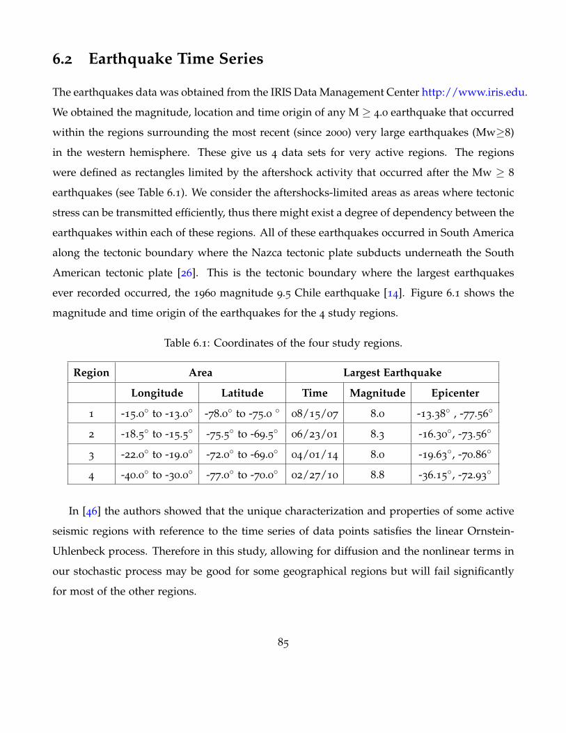
6.2 Earthquake Time Series

The earthquakes data was obtained from the IRIS Data Management Center http://www.iris.edu.

We obtained the magnitude, location and time origin of any M ≥ 4.0 earthquake that occurred

within the regions surrounding the most recent (since 2000) very large earthquakes (Mw≥8)

in the western hemisphere. These give us 4 data sets for very active regions. The regions

were defined as rectangles limited by the aftershock activity that occurred after the Mw ≥ 8

earthquakes (see Table 6.1). We consider the aftershocks-limited areas as areas where tectonic

stress can be transmitted efficiently, thus there might exist a degree of dependency between the

earthquakes within each of these regions. All of these earthquakes occurred in South America

along the tectonic boundary where the Nazca tectonic plate subducts underneath the South

American tectonic plate [26]. This is the tectonic boundary where the largest earthquakes

ever recorded occurred, the 1960 magnitude 9.5 Chile earthquake [14]. Figure 6.1 shows the

magnitude and time origin of the earthquakes for the 4 study regions.

Table 6.1: Coordinates of the four study regions.

Region Area Largest Earthquake

Longitude Latitude Time Magnitude Epicenter

1 -15.0 to -13.0 -78.0 to -75.0 08/15/07 8.0 -13.38 , -77.56

2 -18.5 to -15.5 -75.5 to -69.5 06/23/01 8.3 -16.30, -73.56

3 -22.0 to -19.0 -72.0 to -69.0 04/01/14 8.0 -19.63, -70.86

4 -40.0 to -30.0 -77.0 to -70.0 02/27/10 8.8 -36.15, -72.93

In [46] the authors showed that the unique characterization and properties of some active

seismic regions with reference to the time series of data points satisfies the linear Ornstein-

Uhlenbeck process. Therefore in this study, allowing for diffusion and the nonlinear terms in

our stochastic process may be good for some geographical regions but will fail significantly

for most of the other regions.

85

http://www.iris.edu#hovno2

2000 2005 2010 2015 Time (year)

864864

864

864

Mag

nitu

de

M=8.0

M=8.3

M=8.0

M=8.8

Region 1

Region 2

Region 3

Region 4

Figure 6.1: Magnitude as a function of time origin of earthquakes for the 4 study regions

defined in Table 6.1.

86

6.3 Numerical Simulation and Results

In the numerical study of the time series arising in seismology, we used data collected from

a location at a given time to estimate the magnitude of the earthquakes at a given location,

where the real magnitude is known. The magnitudes recorded in the data set was used.

In the time series data points, the local variance of the series was larger when the level of

the series was higher. We therefore normalized the data sets by taking logarithm of the time

series data points. By performing this change of scale, it is likely that a stationary or integrated

model can be fitted after the transformation (see [21] for details).

The superposed Γ(a, b) Ornstein-Uhlenbeck model is applied to the geophysical time se-

ries as follows. We first estimate the model parameters a, b and λ1 using the relations given

in (3.47) and (3.49) respectively. Next, we simulate data from the superposed Γ(a, b) Ornstein-

Uhlenbeck model following the discussions in Chapter 3 Section 3.5. We simulated indepen-

dent path of our model using different time steps. Finally, we compared the random time

series generated from the superposed Γ(a, b) Ornstein-Uhlenbeck model to the original earth-

quake time series. In order to investigate our model fit, we computed the root mean square

error (RMSE) for each region. The RMSE estimates measure how well our model fits the given

data sets. In this work, we used the RMSE estimates to measure the fit of the random time

series generated from our proposed model and the original earthquake time series observed.

Physical interpretations of the parameters used in our model are as follows. The rate

parameter, a controls the rate of jump arrivals of the earthquake time series. If a is large, then

the time series will be more concentrated; if a is small then it will be more spread out. The

shape or scale parameter, b describes the jump size of the earthquake time series rather than

simply shifting it. λ1 and λ2 are the rate parameters of our superposed Γ(a, b)- Uhlenbeck

model that measures how the model react to perturbations.

87

Table 6.2: Estimation of Parameters: λ1, a, b.

Regions Number of ob-

servations

λ1 a b

Region 1 389 2.1776 158.9808 34.4993

Region 2 1000 3.0955 196.4128 43.2430

Region 3 892 1.6348 151.7649 33.0730

Region 4 5000 1.6344 205.7332 46.0565

Table 6.3: Data Results for superposed Γ(a, b) Ornstein-Uhlenbeck model.

Regions λ1 λ2 w1 w2 RMSE

Region 1 2.1776 2.9776 0.50 0.50 0.1066

Region 2 3.0955 4.6165 0.60 0.40 0.0948

Region 3 1.6348 2.3348 0.45 0.55 0.1017

Region 4 1.6344 2.6344 0.60 0.40 0.0941

6.3.1 Results from analysis of earthquake time series

Results of the earthquake time series for the four (4) regions discussed are presented. Table 6.2

summarizes the results of the estimation of parameters for the superposed Γ(a, b) Ornstein-

Uhlenbeck model.

Table 6.3 and 6.4 summarizes our numerical results for the earthquake time series when the

superposed Γ(a, b) Ornstein-Uhlenbeck model and the ordinary Γ(a, b) Ornstein-Uhlenbeck

model were applied to real earthquake data series respectively. We obtained λ2 by adjusting

λ1 in order to fit the superposed Γ(a, b) Ornstein-Uhlenbeck model.

The RMSE estimates for the random time series generated from the superposed Γ(a, b)

Ornstein-Uhlenbeck model and the original earthquake time series are also presented in Table

6.3. Similarly, the RMSE estimates for the random time series generated from the ordinary

Γ(a, b) Ornstein-Uhlenbeck model and the original earthquake time series are also presented

88

Table 6.4: Data Results for Γ(a, b) Ornstein-Uhlenbeck model.

Regions λ1 RMSE

Region1 2.1776 0.1207

Region2 3.0955 0.1025

Region3 1.6348 0.1030

Region4 1.6344 0.0991

in Table 6.4.

Based on the RMSE estimates obtained in Tables 6.3 and 6.4, it is evident that the super-

posed Γ(a, b) Ornstein-Uhlenbeck model fit well than the ordinary Γ(a, b) Ornstein-Uhlenbeck

model. This is due to the fact that, the superposed Γ(a, b) Ornstein-Uhlenbeck model is a

weighted sum of solutions. Moreover, because the superposed Γ(a, b) Ornstein-Uhlenbeck

model need not be identically distributed, it offers a lot of flexibility in the model.

Figures 6.2, 6.3, 6.4 and 6.5 reports the sample path for the simulated data sets correspond-

ing to Regions 1, 2, 3 and 4. The sample path refers to the path of the simulated superposed

Γ(a, b) Ornstein-Uhlenbeck process. The horizontal axis is time, t and the vertical is the su-

perposed Γ(a, b) Ornstein-Uhlenbeck process, Xt. The path is dominated by jumps and also

illustrates the fact that the process is everywhere continuous and non-negative.

The very good fit of the observed magnitudes of the earthquakes with the stochastic differ-

ential equations, supports the use of this methodology for the study of earthquakes sequence

6.4 Significance of the results obtained

In this chapter, we implemented flexible classes of processes that incorporate long-range

dependence, i.e. they have slow polynomially decaying autocovariance function and self-

similarity like properties and that are capable of describing some of the key distribution

features of typical geophysical time series. In order to capture more realistic dependence

89

Figure 6.2: A Sample Path of the superposed Γ(a, b)-OU process with λ1 = 2.1776, λ2 = 2.9776

, a = 158.9808 and b = 34.4993 for region 1.


, a = 196.4128 and b = 43.2430 for region 2.

90


, a = 151.7649 and b = 33.0730 for region 3.


, a = 205.7332 and b = 46.0565 for region 4.

91

structures, we summed two independent Γ(a, b) Ornstein-Uhlenbeck processes.

We generated random time series from our proposed model; the superposed Γ(a, b) Ornstein-

Uhlenbeck process to estimate the magnitude of the earthquake for the four regions. Look-

ing at the computed model fit; the root mean square error, the superposed Γ(a, b) Ornstein-

Uhlenbeck process gives a good fit. We also compared the random time series generated

from the superposed Γ(a, b) Ornstein-Uhlenbeck process to the random time series generated

from the ordinary Γ(a, b) Ornstein-Uhlenbeck process. In this instance, the superposed Γ(a, b)

Ornstein-Uhlenbeck process gave a better fit than the Γ(a, b) Ornstein-Uhlenbeck process. This

is evident in their RMSE estimates.

In previous works [35] and [7], the authors concluded that the generalized Levy models

where very suitable to describe critical events including earthquakes. The solution to our

stochastic differential equation is a Levy model, so the very good fit obtained reinforces the

previous conclusions. We obtained very good fits of the observed magnitudes of the earth-

quakes with the stochastic differential equations (see Table 6.3), which supports the use of this

modeling methodology for the study of earthquakes sequences.

An important example and potential application of this work is for analyzing the effect

of events that occurred very far in the past, for example decades ago, might have on the

occurrence of present and future events. This type of analysis might help to better understand

how tectonic stress decays and accumulates during long period of time.

92

Chapter 7

Modeling earthquake series dependencies

by using coupled system stochastic

differential equations

In the Chapters 4- 6 of this dissertation, we described the modeling of phenomena by using a

stochastic differential equation in a way that combines the aspects on how present occurrences

will affect future occurrences and also allows for the fact that there will be small random

effects shifting a natural phenomena state in future periods. In reality phenomena such as the

ones described in this dissertation are influenced by random noise thus it is appropriate for

the behavior of the noise to be reflected in the differential equations. Stochastic differential

equations play an important role in applications of different kinds of fields; however in this

study we focus on geophysics.

In this chapter, we model the influence of any natural or physical phenomena and the effect

on each other, by using a coupled system of two stochastic differential equations. We test our

approach and present a numerical example by using real world earthquake series. In this

application, we describe the correlation of earthquake series from four regions in the country

Chile by using coupled system of Γ(a, b) Ornstein-Uhlenbeck stochastic differential equations.

The objective is to model the dependency and effects of earthquake series occurring at four

different regions within the same geographical area.

93

7.1 Background of Earthquake Time Series

The data used in this chapter is the same as the data sets used in Chapter 6 of this book.

However, the novelty of this application is different from that of Chapter 6. In this chapter,

we compare the four regions from the country Chile and simulate data to investigate the

correlation of earthquake series between the regions. In that, we discuss if the occurrence of

earthquake in one region affects the occurrence of another. For completeness of this chapter,

we briefly present the data background.

The earthquakes series used in this study was obtained from the IRIS Data Management

Center http://www.iris.edu. We obtained the magnitude, location and time origin of any M ≥

4.0 earthquake that occurred within the regions surrounding the most recent (since 2000) very

large earthquakes (Mw≥8) in the western hemisphere. These comprised of 4 earthquake series

for four regions shown is Figure 7.1. We consider the aftershocks-limited areas as areas where

tectonic stress can be transmitted efficiently, thus there might exist a degree of dependency

between the earthquakes within each of these regions. All of these earthquakes occurred in

South America along the tectonic boundary where the Nazca tectonic plate subducts under-

neath the South American tectonic plate [26]. This is the tectonic boundary where the largest

earthquakes ever recorded occurred, the 1960 magnitude 9.5 Chile earthquake [14].

Before we proceed to simulate data using our proposed model, we compute the correlation

matrix between the four regions to verify if there exist any form of dependency between the

four regions. The correlation matrix for all the four regions are given below:

Region 1 Region 2 Region 3 Region 4

Region 1 1.00 −0.0046 −0.0089 −0.0386

Region 2 −0.0046 1.00 −0.0464 0.0220

Region 3 −0.0089 −0.0464 1.00 −0.0313

Region 4 −0.0386 0.0220 −0.0313 1.00

Each cell in the table shows the correlation between two regions. The line of 1.00’s going

from the top left to the bottom right is the main diagonal, which shows that each region

94

http://www.iris.edu#hovno2

0

15

30

45-90 -75 -60

0

0

0

0

000

Nazca Plate

SouthAmerican Plate

Pacific Ocean4 6 8Magnitude

0 300 600Depth (Km)

1960, M=9.5

12

3

4

Figure 7.1: Map shows the spatial distribution of earthquakes (colored circles) along the tec-

tonic boundary (red line) between the Nazca and the South American tectonic plates. Red

rectangles represent the four study regions. Inset shows the area in larger map. Color rep-

resents earthquake’s depths. White circles mark the location of the very large earthquakes

(Mw≥8). For reference, white star marks the location of the largest earthquake ever recorded.

95

always perfectly correlates with itself. For example the correlation between regions 1 and 2

is −0.0046 and that between regions 2 and 3 is −0.0464. This matrix is symmetrical with the

same correlation shown above the main diagonal being a mirror image of those below the main

diagonal. From the above matrix, we observe that there exist some correlation between the

four regions therefore it is appropriate to model the earthquake series by using our proposed

coupled system.

7.2 Application

In this section, we present the numerical results of the geophysical time series arising in

seismology. The earthquake series from the four regions constituted data collected from a

location at a given time to estimate the magnitude of the earthquakes at a given location,

where the real magnitude is known. The earthquake magnitudes recorded in the data set was

used in our analysis.

One charecteristics of the earthquake series data points is that, the local variance of the

series was larger when the level of the series was higher. We therefore transformed the data

into a different scale by taking logarithm of the time series data points. By performing this

change of scale, it is likely that a stationary model can be fitted after the transformation (see

[21] for details).

The 2-dimensional Γ(a, b) Ornstein-Uhlenbeck model is applied to the earthquake series as

follows. We first estimate the model parameters a, b and λ corresponding to each region by

using the relations given in (3.47) and (3.49) respectively.

Next, we simulate data from the our model following the discussions in Chapter 3 Section

3.5. We simulated independent path of our model using different time steps. Finally, we com-

pared the simulated time series generated from the 2-dimensional Γ(a, b) Ornstein-Uhlenbeck

model to the original earthquake time series. In order to investigate our model fit, we com-

puted the root mean square error (RMSE) for all the four regions in Chile. The RMSE estimates

measure how well our proposed model fits the original earthquake time series.

96

Table 7.1: Data and parameter estimates

Regions Number of

observations

X0 λ a b

Region 1 389 4.70 2.1776 158.9808 34.4993

Region 2 1000 5.00 3.0955 196.4128 43.2430

Region 3 892 5.00 1.6348 151.7649 33.0730

Region 4 5000 4.70 1.6344 205.7332 46.0565

7.3 Results

The numerical results of the earthquake time series for the four (4) regions discussed are

presented. Table 7.1 summarizes the numerical results of the estimation of parameters for

four regions understudy. In the table, the second and third column represents the number of

data points represents and initial points X0 for the earthquake time series. The fourth, fifth

and sixth columns in Table 7.1 represents the estimated parameters from real data.

Table 7.2 summarizes the numerical results for the earthquake time series when the 2-

dimensional Γ(a, b) Ornstein-Uhlenbeck model was applied to real earthquake data series. In

the table the parameters σ11 and σ22 corresponds to the volatility of our earthquake time series

and σ12 and σ21 describes the correlation between the regions understudy. For example, the

results displayed in the first row of Table 7.2, represents coupled system of processes between

Regions 1 and 2. In this scenario, we modeled the two regions as a coupled system where

the occurrence of earthquake at one region has an effect on the occurrence of earthquake at

another. From the table, we observed that for all the coupled regions, the values for σ12 = σ21

and all these values were different from zero. We recall that if σ12 = σ21 = 0, then there exist

no correlation between the regions understudy.

The error estimates for the random time series generated our 2-dimensional stochastic

model and the original earthquake time series are also presented in Table Table 7.2. We observe

that two error estimates are estimated in Table 7.2. The first estimate is when the simulated

97

Table 7.2: Data Results for 2-dimensional Γ(a, b) Ornstein-Uhlenbeck model.

Regions σ11 σ12 σ21 σ22 RMSE 1 RMSE 2

Region

1 and

Region 2

0.5168 -0.0046 -0.0046 0.4583 0.3736 0.3563

Region

1 and

Region 3

0.5168 -0.0089 -0.0089 0.5514 0.1576 0.20630

Region

1 and

Region 4

0.5168 -0.0386 -0.0386 0.4411 0.1189 0.2733

Region

2 and

Region 3

0.4389 -0.0464 -0.0464 0.5514 0.3774 0.5997

Region

2 and

Region 4

0.4389 0.0220 0.0220 0.4411 0.31251 0.22890

Region

3 and

Region 4

0.5514 -0.0313 -0.0313 0.4411 0.2499 0.3374

98

results arising from the first region is compared with the actual time series and the second

estimate is when the the simulated results arising from the second region is compared with

the actual time series from that same region. One interesting property with this results is the

fact that, the results where generated from a coupled system. The results obtained indicate

that the stochastic differential equation model provides a reasonable fit to the earthquake data.

Figures 7.2–7.7, reports the sample path for the simulated earthquake time series for the

coupling regions. In the figures, the black colored path represents the sample path originating

from the first stochastic differential equation X1(t) and the red colored path represents the

sample path originating from the second stochastic differential equation X2(t). The path is

dominated by jumps and also illustrates the fact that the process is everywhere continuous

and non-negative.

Figure 7.2: Sample Path of the coupled stochastic model for regions 1 and 2.

99



100



101


7.4 Concluding remarks

In the chapter, we modeled the correlation of earthquake series from four regions in the coun-

try Chile by using coupled system of Γ(a, b) Ornstein-Uhlenbeck Stochastic Differential Equa-

tions. The goal is to model the dependency and effects of earthquake series occurring at all

the regions and determine if the occurrence of earthquake at one region has the effect an effect

on the another region. The modeling approached used here is very similar to the work by

the authors in Ref. [37] except the fact that in this study we considered coupled system of

stochastic differential equations. Based on the results obtained the proposed model provides

a reasonable fit to the earthquake data. The selection of this model is justifiable since from

the correlation matrix obtained from all the four earthquake series in the country Chile, there

exist some dependency between the occurrences of earthquakes.

102

Chapter 8

Conclusion

In this dissertation we introduced a new method of the modeling and statistical analysis of

complex time series to enhance the understanding of extreme events. By using the super-

position and coupling system of Γ(a, b) Ornstein-Uhlenbeck stochastic differential equation,

we showed that proposed method accurately describes the behavior of financial indices and

earthquake series due to two essential property: firstly, the model is completely stochastic and

secondly, the method takes into account the physical behavior of the time series when mod-

eling the data. This was proved and justified using the Γ(a, b) Ornstein-Uhlenbeck process.

We compared the results from our proposed model with those derived from different meth-

ods currently adopted to model financial and geophysical time series. Most of the traditional

models have in common the fact that they are based upon the Gaussian assumption. However,

the empirical study of some financial indices shows that in short time intervals the associated

probability density function has greater kurtosis than a Gaussian distribution [4, 30]. In addi-

tion the models described in previous literature fails to take into account the behavior of the

financial and earthquake data, and some of the models are not completely stochastic.

In this dissertation, we implemented very flexible classes of processes that incorporate

long-range dependence, i.e. they have a slowly polynomially decaying autocovariance func-

tion and self-similarity like properties that are capable of describing some of the key distri-

butional features of typical financial and geophysical time series. In order to capture realistic

dependence structures, we combined independent Ornstein-Uhlenbeck processes driven by a

Levy process. In addition to model the correlation between different regions in lying in the

same geographical area where an earthquake series was recorded we used coupled system of

independent Ornstein-Uhlenbeck processes driven by a Levy process. These selection process

103

is supported by the fact that generalized Levy models are suitable for describing these type of

time series [34]. Furthermore, the benefits of using the superposed and coupled system of in-

dependent Ornstein-Uhlenbeck processes is that the model offers plenty of analytic flexibility

which is not available for more standard models such as the geometric Gaussian Ornstein-

Uhlenbeck processes. In addition, the superposition of Ornstein-Uhlenbeck processes provide

a class of continuous time processes capable of exhibiting long memory behavior. The presence

of long memory suggests that current information is highly correlated with past information

at different levels.

This dissertation focuses on theory and on application, as a way to check the efficiency

of the new method of analysis. The efficiency of the superposed and coupled system of

Γ(a, b) Ornstein-Uhlenbeck processes were illustrated by showing this analysis in action on

real complex data, that is, financial and geophysical time series. The financial time series

used comprised of two frequency; moderate frequency (daily) and high frequency (minute

and second). The geophysical time series also consisted of high frequency earthquake time

series. Based on the computed model fit; the root mean square error, the proposed Γ(a, b)

Ornstein-Uhlenbeck stochastic differential equation gives a good fit. This is because the sim-

ulated results is very similar to the actual realizations. Additionally, the model parameters

obtained from our statistical analysis are very useful for making inferences and predictions.

For example the intensity parameters λ1 and λ2 describes the mean reversion speed of the

specific time series and explains how our model reacts to perturbation. From the analysis in

Chapter 5, we observe that the intensity parameters for the second by second high frequency

times series are smaller compared to the minute by minute high frequency time series. This

results suggests that in the long run, the closing prices for the stock exchanges of the minute

by minute data will approach its mean closing prices faster than the second by second data.

The results obtained will give an idea of the statistics of the future stock paths. This will help

investors or practitioners who lacks insider information but has at their disposal all the infor-

mation contained in the equity prices discover that a crash is imminent and take the necessary

precautions. From the geophysical point of view, the results obtained will describe how the

104

effect of events that occurred very far in the past, for example decades ago, might have on the

occurrence of present and future events. This type of analysis might help to better understand

how tectonic stress decays and accumulates during long period of time. Based on the results of

this dissertation, we conclude that the superposed and system of Γ(a, b) Ornstein-Uhlenbeck

stochastic differential equation accurately detect the statistical and temporal properties of the

financial and geophysical time series. Several application in data science, statistics and related

disciplines will be discussed in future work. Another future work will be to investigate the

time an awareness should be raised for a high magnitude earthquake or market crash.

105

References

[1] S. Ahmad and A. Ambrosetti. A Textbook on Ordinary Differential Equations. Springer, 2014.

[2] D. Applebaum. Levy processes and Stochastic Calculus. Cambridge University Press, 2004.

[3] A. Arikoglu and I. Ozkol. Solutions of integral and integro-differential equation sys-

tems by using differential transform method. Computers & Mathematics with Applications,

56(9):2411–2417, 2008.

[4] R.T. Baillie and T. Bollerslev. Common stochastic trends in a system of exchange rates.

Journal of Finance, 44:167–181, 1989.

[5] S. Bar-Lev, D. Bshouty, and G. Letac. Natural exponential families and self-

decomposability. Statistics and Probability Letters, 13:147–152, 1992.

[6] E. Barany, M.P. Beccar-Varela, I. Florescu, and I. SenGupta. Detecting market crashes by

analyzing long memory effects using high frequency data. Quantitative Finance, 12(4):623–

634, 2011.

[7] E. Barany, M.P. Beccar-Varela, I. Florescu, and I. SenGupta. Detecting market crashes by

analyzing long memory effects using high frequency data. Quantitative Finance, 12(4):623–

634, 2011.

[8] O.E. Barndorff-Nielsen and N. Shephard. A finite difference scheme for partial integro-

differential equations with a weakly singular kernel. Applied Numerical Mathematics,

11(4):309–319, 1993.

[9] O.E. Barndorff-Nielsen and N. Shephard. Non-gaussian ornsteinuhlenbeck-based models

and some of their uses in financial economics. Journal of the Royal Statistical Society B,

3:167–241, 2001.

106

[10] M.P. Beccar-Varela, M.C. Mariani, O.K. Tweneboah, and I. Florescu. Analysis of the

lehman brothers collapse and the flash crash event by applying wavelets methodologies.

Physica A, 474:162–171, 2017.

[11] P. Blanchard, R.L. Devaney, and G.L. Hall. Differential Equations. Brooks/Cole Cengage

Learning, 2002.

[12] S. Bochner. Diffusion equation and stochastic processes. Proceedings of the National

Academy of Sciences, U.S.A, 35(7):368–370, 1949.

[13] G. Casella and R. L. Berger. Statistical inference. Duxbury advanced series in statistics and

decision sciences, Thomson Learning, 2002.

[14] M. Cisternas, B. Atwater, F. Torrejn, Y. Sawai, G. Machuca, M. Lagos, A. Eipert, C. Youlton,

I. Salgado, T. Kamataki, M. Shishikura, C. Rajendran, J. Malik, Y. Rizal, and M. Husni.

Predecessors of the giant 1960 chile earthquake. Nature, 437(7057):404–407, 2005.

[15] G.R. Dargahi-Noubary. Stochastic modeling based on deterministic formulation: An ex-

ample. Mathematical Geology, 24:161–169, 1992.

[16] B. Delouis, N. JeanMathieu, and M. Valle. Slip distribution of the february 27, 2010 mw=

8.8 maule earthquake, central chile, from static and highrate gps, insar, and broadband

teleseismic data. Geophysical Research Letters, 37(17), 2010.

[17] D. Easley, M. Lopez de Prado, and M. O’Hara. The microstructure of the ‘flash crash’:

Flow toxicity, liquidity crashes and the probability of informed trading. The Journal of

Portfolio Management, 37:118–128, 2011.

[18] History.com Editors. Bear stearns collapses, sold to j.p. morgan chase. Available

at https://www.history.com/this-day-in-history/bear-stearns-sold-to-j-p-morgan-chase,

2018.

107

https://www.history.com/this-day-in-history/bear-stearns-sold-to-j-p-morgan-chase#hovno2

[19] M. Ferraro, N. Furman, Y. Liu, M.C. Mariani, and D. Rial. Analysis of intermittence, scale

invariance and characteristic scales in the behavior of major indices near a crash,. Physica

A, 359:576, 2006.

[20] I. Florescu. Probability and Stochastic Processes. John Wiley & Sons, 1996.

[21] Research Gate. Available at http://www.researchgate.net/profile/IgnacioArbues/topics.

[22] P. Glasserman. Monte Carlo Methods in Financial Engineering., volume 53 of Stochastic

Modelling and Applied Probability. Springer New York, 2010, 2004.

[23] N. Hautsch. Modelling Irregularly Spaced Financial Data Theory and Practice of Dynamic

Duration Models. Springer-Verlag, 2004.

[24] Z. J. Jurek and W. Vervaat. An integral representation for self-decomposable banach

space valued random variables. Zeitschrift fur Wahrscheinlichkeisheorie and verwandte Gebi-

ete, 62:247–262, 1983.

[25] B. Kalayci. Identification of coupled systems of stochastic differential equations in finance

including investor sentiment by multivariate adaptive regression splines. OpenMETU

Collection for Middle East Technical University, 2017.

[26] H. Kanamori. The energy release in great earthquakes. Journal of Geophysical Research,

82(20:2981–2987, 1977.

[27] H. Kinateder and N. Wagner. Market risk prediction under long memory: When var is

higher than expected. Journal of Risk Finance, 15:4–32, 2014.

[28] D. Lamberton and B. Lapeyre. Introduction to stochastic calculus applied to finance. CRC

press, 2007.

[29] S. Lennartz, V. N. Livina, A. Bunde, and S. Havlin. Long-term memory in earthquakes

and the distribution of interoccurrence times. EPL, 81(6):69001, 2008.

108

http://www.researchgate.net/profile/IgnacioArbues/topics#hovno2

[30] R.N. Mantegna and H.E. Stanley. Scaling behaviour in the dynamics of an economic

index. Nature, 376:46–49, 1995.

[31] M.C. Mariani, P. Bezdek, L. Serpa, and I. Florescu. Ising type models applied to geo-

physics and high frequency market data. Physica A, 390(23):4396–4402, 2011.

[32] M.C. Mariani, M.A.M. Bhuiyan, and O.K. Tweneboah. Stochastic differential equations

applied to the study of geophysical and financial time series. Physica A, 491(1):167–176,

2018.

[33] M.C. Mariani, I. Florescu, M.P. Beccar-Varela, and E. Ncheuguima. Long correlations and

levy models applied to the study of memory effects in high frequency (tick) data. Physica

A, 388(8):1659–1664, 2009.

[34] M.C. Mariani, I. Florescu, I. Sengupta, M. P. Beccar-Varela, P. Bezdek, and L. Serpa. Levy

models and scale invariance properties applied to geophysics. Physica A: Statistical Me-

chanics and its Applications, 392:824–839, 2013.

[35] M.C. Mariani and Y. Liu. Normalized truncated levy walks applied to the study of finan-

cial indices. Physica A, 377:590–598, 2006.

[36] M.C. Mariani and O.K. Tweneboah. Estimation of stochastic volatility by using ornstein-

uhlenbeck type models. Physica A, 443:170–178, 2016.

[37] M.C. Mariani, O.K. Tweneboah, H. Gonzalez-Huizar, and L.F. Serpa. Stochastic differen-

tial equation of earthquakes series. Pure and Applied Geophysics, 173(7):2357–2364, 2016.

[38] G. Maruyama. Continuous markov processes and stochastic equations. Rend Circ Math

Palermo, 4:48–90, 1955.

[39] D. Melgar, W. Fan, S. Riquelme, J. Geng, C. Liang, M. Fuentes, and E. J. Fielding. Slip

segmentation and slow rupture to the trench during the 2015, mw8. 3 illapel, chile earth-

quake. Geophys. Res. Lett., 43:961 966, 2016.

109

[40] T. Mikosch. Elementary stochastic calculus with Finance in view. World Scientific Publishing

Co. Pte. Ltd., 1998.

[41] G.N. Milstein. Approximate integration of stochastic differential equations. Teor. Veroyat-

nost. i Primenen., 19(3):583–588, 1974.

[42] M. Moreno, M. Rosenau, and O. Oncken. 2010 maule earthquake slip correlates with

pre-seismic locking of andean subduction zone. Nature, 467(7312):198–202, 2010.

[43] B. Oksendal. Stochastic Differential Equations: An Introduction with Applications. Springer-

Verlag, 2010.

[44] S.T.G Raghu-Kanth and B. Kavitha. Stochastic finite fault modeling of subduction zone

earthquakes in northeastern india. Int. J. Theor. Appl. Financ., 170:17051727, 2013.

[45] S.M. Ross. Stochastic processes. John Wiley & Sons, 1996.

[46] Habtemicael S. and I. SenGupta. Ornstein-uhlenbeck processes for geophysical data anal-

ysis. Physica A, 399:147–156, 2014.

[47] K. Sato. Levy processes. Cambridge University Press, 1996.

[48] K. Sato. Levy processes and Infinitely Divisible Distributions. Cambridge University Press,

1999.

[49] K. Sato. Levy process in Finance: Pricing Financial Derivatives. Wiley Series in Probability

and Stochastics, 2003.

[50] W. Schoutens and J. Cariboni. Levy processes in Credit Risk. John Wiley & Sons, 2009.

[51] M. Scott. Applied stochastic processes in science and engineering. Available at

http://www.math.uwaterloo.ca/ mscott/Notes.pdfS, 2013.

[52] K. Spiliopoulos. Method of moments estimation of ornstein-uhlenbeck processes driven

by general levy process. ANNALES de l’I.S.U.P., 53:3–19, 2009.

110

http://www.math.uwaterloo.ca/~mscott/Notes.pdfS#hovno2

[53] W.A. Strauss. Partial Differential Equations. John Wiley & Sons, 2008.

[54] T. Tang. A finite difference scheme for partial integro-differential equations with a weakly

singular kernel. Applied Numerical Mathematics, 11(4):309–319, 1993.

[55] O.K. Tweneboah. Stochastic differential equation applied to high frequency data arising

in geophysics and other disciplines. ETD Collection for University of Texas, El Paso, Paper

AAI1600353, 2015.

[56] G.E. Uhlenbeck and L.S. Ornstein. On the theory of the brownian motion. Physical Review,

36:823–842, 1930.

[57] C. Vigny, A. Socquet, J.C. Ruegg, M. Metois, R. Madariaga, S. Morvan, R. Lacassin, J. Cam-

pos, D. Carrizo, M. Bejar-Pizarro, Barrientos S., and Armijo R. The 2010 mw 8.8 maule

megathrust earthquake of central chile, monitored by gps. Science, 332:1417–1421, 2011.

[58] Wikipedia. Stock market crash. Available at https://en.wikipedia.org/wiki/Stock market crash,

2020.

[59] P. Willmott, J.N. Dewynne, and S.D. Howison. Option Pricing: Mathematical Models and

Computation. Oxford Financial Press, Oxford, 1993.

[60] C. Zhang, T. Sato, and L. Lu. A phase model of earthquake motions based on stochastic

differential equation. KSCE Journal of Civil Engineering, 15(1):161–166, 2011.

111

https://en.wikipedia.org/wiki/Stock_market_crash#hovno2

Curriculum Vitae

Osei Kofi Tweneboah is a PhD Candidate in the Computational Science Program at the Uni-

versity of Texas at El Paso (UTEP). In August 2015, he earned a Master of Science degree

in Mathematics from UTEP under the guidance of Prof. Maria C. Mariani. Prior to his en-

rollment in UTEP, He obtained a Bachelor of Science degree in Mathematics from Kwame

Nkrumah University of Science and Technology, Kumasi, Ghana.

While pursuing his PhD in Computational Science he worked as a Teaching and Research

Assistant at the Computational Science Program and Mathematical Sciences department at

UTEP and also as an adjunct faculty at El Paso Community College. Osei has coauthored

sixteen (16) papers in Peer-Reviewed Journals and has co-presented 28 research papers and

posters. Based on his outstanding academic performance, the College of Science at the Univer-

sity of Texas at El Paso awarded him the Academic and Research Excellence Graduate Student

award in Mathematics in May 2015. He has also won many research and travel grants from

the Computational Sciences Program, Department of Mathematical Sciences, UTEP College of

Science, and the UTEP Graduate School.

Osei was the President and Co-founder of the African Students Organization and Com-

putational Science at the University of Texas at El Paso during the 2018-2019 and 2016-2018

academic years respectively. After graduation, Osei will pursue a career in a research univer-

sity as a professor and or a career in the industry.

Contact Email: [email protected]

112

Documents

Applications Of Ornstein-Uhlenbeck Type Stochastic