Embed Size (px)
DESCRIPTION
Octopus
Citation preview
Version 4.1.2
(From the OctopusWiki)
Alberto CastroAngel RubioCarlo Andrea RozziFlorian LorenzenHeiko AppelMicael OliveiraMiguel A. L. MarquesXavier Andrade - David A. Strubbe
The_Octopus_Manual
1
Contents
1 About This Manual1.1 Copying♦ 1.2 Reading this manual♦ 1.3 Getting help♦ 1.4 Contributing♦
•
2 About Octopus2.1 Developers♦ 2.2 Introduction♦ 2.3 History♦ 2.4 Contributing to Octopus♦ 2.5 The Octopus Copying Conditions♦
•
3 Installation3.1 Instructions for Specific Architectures♦ 3.2 Dowloading
3.2.1 Binaries◊ 3.2.2 Source code◊
♦
3.3 Building3.3.1 Quick instructions◊ 3.3.2 Slow instructions◊ 3.3.3 Long instructions
3.3.3.1 Requirements⋅ 3.3.3.2 Optional libraries⋅ 3.3.3.3 Unpacking the sources⋅ 3.3.3.4 Development version⋅ 3.3.3.5 Configuring⋅ 3.3.3.6 Compiling and installing⋅ 3.3.3.7 Testing your build⋅
◊
♦
•
4 Basics4.1 The input file
4.1.1 Input file◊ 4.1.2 Scalar Variables◊ 4.1.3 Mathematical expressions◊ 4.1.4 Predefined variables◊ 4.1.5 Blocks◊ 4.1.6 Comments◊ 4.1.7 Default values◊ 4.1.8 Documentation◊ 4.1.9 Experimental features◊ 4.1.10 Good practices◊
♦
4.2 Running Octopus4.2.1 Input◊ 4.2.2 Executing◊ 4.2.3 Output◊ 4.2.4 Clean Stop◊ 4.2.5 Restarting◊
♦
4.3 Units♦
•
The_Octopus_Manual
Contents 2
4.3.1 Atomic Units◊ 4.3.2 Convenient Units◊ 4.3.3 Units in Octopus◊ 4.3.4 Mass Units◊ 4.3.5 Charge Units◊ 4.3.6 Unit Conversions◊
4.4 Physical System♦ 4.5 Dimensions♦ 4.6 Species
4.6.1 Pseudopotentials◊ 4.6.2 All-Electron Nucleus◊ 4.6.3 User Defined◊
♦
4.7 Coordinates♦ 4.8 Velocities♦ 4.9 Number of Electrons♦ 4.10 Hamiltonian♦ 4.11 Introduction
4.11.1 Ground-State DFT◊ 4.11.2 Time-dependent DFT◊
♦
4.12 Occupations♦ 4.13 External Potential♦ 4.14 Electron-Electron Interaction
4.14.1 Exchange and correlation potential◊ ♦
4.15 Relativistic Corrections4.15.1 Spin-orbit Coupling◊
♦
4.16 Discretization♦ 4.17 Grid
4.17.1 Double grid (experimental)◊ ♦
4.18 Box4.18.1 Zero boundary conditions◊
♦
4.19 Output4.19.1 Ground-State DFT◊ 4.19.2 Time-Dependent DFT
4.19.2.1 Optical Properties⋅ 4.19.2.2 Linear-Response Theory⋅ 4.19.2.3 Electronic Excitations byMeans of Time-Propagation
⋅
◊
4.19.3 References◊
♦
4.20 Troubleshooting4.20.1 Read parser.log◊ 4.20.2 Use OutputDuringSCF◊ 4.20.3 Set DebugLevel◊
♦
4.21 Symmetry♦ 5 Calculations
5.1 Ground State♦ 5.2 Kohn-Sham Ground State
5.2.1 Mixing◊ 5.2.2 Convergence◊
♦
•
The_Octopus_Manual
Contents 3
5.2.3 Eigensolver◊ 5.2.4 LCAO◊
5.3 Unoccupied states♦ 5.4 Time-Dependent
5.4.1 Time evolution5.4.1.1 Propagators for thetime-dependent Kohn-Sham equations
5.4.1.1.1 Splitting techniques• 5.4.1.1.2 Midpoint rules• 5.4.1.1.3 Magnus expansions• 5.4.1.1.4Time-reversal-symmetry basedpropagation
•
⋅
5.4.1.2 Approximations to theexponential of an operator
5.4.1.2.1 Polynomial expansions• 5.4.1.2.2 Krylov-subspaceprojection
•
5.4.1.2.3 Splitting techniques•
⋅
◊
5.4.2 Performing a time-propagation◊ 5.4.3 External fields
5.4.3.1 Delta kick: Calculating anabsorption spectrum
⋅
5.4.3.2 Lasers⋅
◊
5.4.4 Symmetries◊
♦
5.5 Casida Linear Response♦ 5.6 Sternheimer Linear Response
5.6.1 Ground state◊ 5.6.2 Input◊ 5.6.3 Output◊ 5.6.4 Finite differences◊
♦
5.7 Optimal Control♦ 5.8 Theoretical Introduction♦ 5.9 Population target: scheme of Zhu, Botina andRabitz
♦
5.10 The asymmetric double well: preparing the states♦ 5.11 Running octopus in QOCT mode♦ 5.12 Analysis of the results♦ 5.13 References♦ 5.14 Geometry Optimization♦
6 Advanced ways of running Octopus6.1 Parallel Octopus
6.1.1 Parallel in States◊ 6.1.2 Parallel in Domains◊ 6.1.3 Problems with parallelization◊ 6.1.4 Compiling and running in parallel◊
♦
6.2 Multi-Dataset Mode♦ 6.3 Passing arguments from environment variables♦
•
The_Octopus_Manual
Contents 4
6.3.1 Examples◊ 7 Utilities
7.1 oct-atomic_occupations7.1.1 Options◊ 7.1.2 Examples◊
♦
7.2 oct-casida_spectrum7.2.1 NAME◊ 7.2.2 SYNOPSIS◊ 7.2.3 DESCRIPTION◊ 7.2.4 AUTHOR◊ 7.2.5 REPORTING BUGS◊ 7.2.6 COPYRIGHT◊ 7.2.7 SEE ALSO◊
♦
7.3 oct-center-geom7.3.1 NAME◊ 7.3.2 SYNOPSIS◊ 7.3.3 DESCRIPTION◊ 7.3.4 AUTHOR◊ 7.3.5 REPORTING BUGS◊ 7.3.6 COPYRIGHT◊ 7.3.7 SEE ALSO◊
♦
7.4 oct-propagate_spectrum7.4.1 NAME◊ 7.4.2 SYNOPSIS◊ 7.4.3 DESCRIPTION◊ 7.4.4 AUTHOR◊ 7.4.5 REPORTING BUGS◊ 7.4.6 COPYRIGHT◊ 7.4.7 SEE ALSO◊
♦
7.5 oct-display_partitions7.5.1 NAME◊ 7.5.2 SYNOPSIS◊ 7.5.3 DESCRIPTION◊ 7.5.4 AUTHOR◊ 7.5.5 REPORTING BUGS◊ 7.5.6 COPYRIGHT◊ 7.5.7 SEE ALSO◊
♦
7.6 oct-harmonic-spectrum7.6.1 NAME◊ 7.6.2 SYNOPSIS◊ 7.6.3 DESCRIPTION◊ 7.6.4 AUTHOR◊ 7.6.5 REPORTING BUGS◊ 7.6.6 COPYRIGHT◊ 7.6.7 SEE ALSO◊
♦
7.7 oct-vibrational_spectrum♦ 7.8 oct-rotatory_strength
7.8.1 NAME◊ ♦
•
The_Octopus_Manual
Contents 5
7.8.2 SYNOPSIS◊ 7.8.3 DESCRIPTION◊ 7.8.4 AUTHOR◊ 7.8.5 REPORTING BUGS◊ 7.8.6 COPYRIGHT◊ 7.8.7 SEE ALSO◊
7.9 oct-run_periodic_table7.9.1 NAME◊ 7.9.2 SYNOPSIS◊ 7.9.3 DESCRIPTION◊ 7.9.4 EXAMPLES◊ 7.9.5 AUTHOR◊ 7.9.6 REPORTING BUGS◊ 7.9.7 COPYRIGHT◊ 7.9.8 SEE ALSO◊
♦
7.10 oct-run_regression_test.pl7.10.1 NAME◊ 7.10.2 SYNOPSIS◊ 7.10.3 DESCRIPTION◊ 7.10.4 EXAMPLES◊ 7.10.5 AUTHOR◊ 7.10.6 REPORTING BUGS◊ 7.10.7 COPYRIGHT◊ 7.10.8 SEE ALSO◊
♦
7.11 oct-run_testsuite7.11.1 NAME◊ 7.11.2 SYNOPSIS◊ 7.11.3 DESCRIPTION◊ 7.11.4 EXAMPLES◊ 7.11.5 AUTHOR◊ 7.11.6 REPORTING BUGS◊ 7.11.7 COPYRIGHT◊ 7.11.8 SEE ALSO◊
♦
7.12 oct-xyz-anim7.12.1 NAME◊ 7.12.2 SYNOPSIS◊ 7.12.3 DESCRIPTION◊ 7.12.4 AUTHOR◊ 7.12.5 REPORTING BUGS◊ 7.12.6 COPYRIGHT◊ 7.12.7 SEE ALSO◊
♦
7.13 Visualization7.13.1 dx◊ 7.13.2 XCrySDen◊ 7.13.3 CUBE◊
♦
7.14 Deprecated Utilities7.14.1 octopus_cmplx◊ 7.14.2 oct-sf◊
♦
The_Octopus_Manual
Contents 6
7.14.3 oct-hs-mult and oct-hs-acc◊ 7.15 oct-rs *♦ 7.16 oct-excite *♦ 7.17 oct-make-st *♦ 7.18 oct-convert *
7.18.1 Name◊ 7.18.2 Description◊ 7.18.3 Example◊
♦
7.19 oct-help7.19.1 search◊ 7.19.2 show◊
♦
8 Examples8.1 Hello World
8.1.1 Exercises◊ ♦
8.2 Benzene♦
•
9 Variables9.1 td_occup♦
•
10 Appendix10.1 Appendix: Updating to a new version
10.1.1 Octopus 4.110.1.1.1 Installation⋅ 10.1.1.2 Restart files⋅
◊
10.1.2 Octopus 4.010.1.2.1 Installation⋅ 10.1.2.2 Variables⋅ 10.1.2.3 Utilities⋅
◊
10.1.3 Octopus 3.010.1.3.1 Input variables⋅ 10.1.3.2 Output directories⋅ 10.1.3.3 Restart file format⋅ 10.1.3.4 Recovering old restart files⋅
◊
♦
10.2 Appendix: Building from scratch10.2.1 Prerequisites◊ 10.2.2 Compiler flags◊ 10.2.3 Compilation of libraries
10.2.3.1 BLAS⋅ 10.2.3.2 LAPACK⋅ 10.2.3.3 GSL⋅ 10.2.3.4 FFTW 3⋅ 10.2.3.5 LibXC⋅
◊
10.2.4 Compilation of Octopus◊
♦
10.3 Appendix: Octopus with GPU support10.3.1 Consideration before using a GPU
10.3.1.1 Calculations that will beaccelerated by GPUs
⋅
10.3.1.2 Supported GPUs⋅ 10.3.1.3 Activating GPU support⋅
◊
10.3.2 Starting the tutorial: running without◊
♦
•
The_Octopus_Manual
Contents 7
OpenCL10.3.3 Selecting the OpenCL device◊ 10.3.4 The block-size◊ 10.3.5 StatesPack◊ 10.3.6 The Poisson solver◊
10.4 Appendix: Specific architectures♦ 11 Generic Ubuntu 10.10• 12 Generic MacOS• 13 United States
13.1 Sequoia/Vulcan (IBM Blue Gene/Q)♦ 13.2 Stampede♦ 13.3 Edison♦ 13.4 Hopper♦ 13.5 Titan♦ 13.6 Kraken♦ 13.7 Lonestar♦ 13.8 Lawrencium♦
•
14 Europe14.1 Curie
14.1.1 PFFT 1.0.5 and BigDFT 1.6.0◊ 14.1.2 PFFT 1.0.7 and BigDFT 1.7.0◊
♦
14.2 Fermi/Juqueen♦ 14.3 Hydra♦ 14.4 Jugene♦ 14.5 Finis Terrae♦ 14.6 MareNostrum II♦ 14.7 MareNostrum III♦ 14.8 Green♦ 14.9 Corvo♦ 14.10 LaPalma♦ 14.11 Appendix: Porting Octopus and PlatformSpecific Instructions
14.11.1 General information and tips aboutcompilers
◊
14.11.2 SSE2 support◊ 14.11.3 Operating systems
14.11.3.1 Linux⋅ 14.11.3.2 Solaris⋅ 14.11.3.3 Tru 64⋅ 14.11.3.4 Mac OS X⋅ 14.11.3.5 Windows⋅
◊
14.11.4 Compilers14.11.4.1 Intel Compiler forx86/x86_64
⋅
14.11.4.2 Intel Compiler for Itanium⋅ 14.11.4.3 Open64⋅ 14.11.4.4 Pathscale Fortran Compiler⋅ 14.11.4.5 NAG compiler⋅
◊
♦
•
The_Octopus_Manual
Contents 8
14.11.4.6 GNU C Compiler (gcc)⋅ 14.11.4.7 GNU Fortran (gfortran)⋅ 14.11.4.8 g95⋅ 14.11.4.9 Portland 6⋅ 14.11.4.10 Portland 7, 8, 9⋅ 14.11.4.11 Portland 10⋅ 14.11.4.12 Portland 11⋅ 14.11.4.13 Portland 12⋅ 14.11.4.14 Absoft⋅ 14.11.4.15 Compaq compiler⋅ 14.11.4.16 Xlf⋅ 14.11.4.17 SGI MIPS⋅ 14.11.4.18 Sun Studio⋅
14.11.5 MPI Implementations14.11.5.1 OpenMPI⋅ 14.11.5.2 MPICH2⋅ 14.11.5.3 SGI MPT⋅ 14.11.5.4 Intel MPI⋅ 14.11.5.5 Sun HPC ClusterTools⋅ 14.11.5.6 MVAPICH⋅
◊
14.11.6 NetCDF◊ 14.11.7 BLAS and LAPACK
14.11.7.1 AMD ACML⋅ 14.11.7.2 ATLAS⋅ 14.11.7.3 Compaq CXML⋅ 14.11.7.4 [GOTO BLAS]⋅ 14.11.7.5 Intel MKL⋅ 14.11.7.6 Netlib⋅
◊
14.12 Appendix: Reference Manual♦ 14.13 Appendix: Copying
14.13.1 INTRODUCTION◊ 14.13.2 LICENSE EXCEPTIONS◊ 14.13.3 Expokit◊ 14.13.4 Metis 4.0
14.13.4.1 METIS COPYRIGHTNOTICE
⋅ ◊
14.13.5 qshep14.13.5.1 QSHEP COPYRIGHTNOTICE
⋅ ◊
♦
If you are going to collaborate, please check Writing Documentation.If you want to know what you can do check for open tickets: [1]If you want to print or download the whole manual there is a PDF version available.
The_Octopus_Manual
Contents 9
About This Manual
Copying
This manual is for Octopus 4.1.2, a first principles, electronic structure, excited states, time-dependentdensity functional theory program.
Copyright © 2006 Miguel A. L. Marques, Xavier Andrade, Alberto Castro and Angel Rubio
Permission is granted to copy, distribute and/or modify this document under the terms of the GNU FreeDocumentation License, Version 1.1 or any later version published by the Free Software Foundation; with noInvariant Sections, no Front-Cover Texts, and no Back-Cover Texts.
You can find a copy of the Free Documentation License here
Reading this manual
If you are new to Octopus it is recommended that you read this manual sequentially. To read this manual you needsome basic knowledge of Density Functional Theory (DFT) and Time Dependent Density Functional Theory(TDDFT), also a bit of numerical methods may be useful.
The way to tell what to do Octopus is through input variables, each one of this variable has its properdocumentation describing what it does and what are the possible values that it can take. All this documentation ofthe variables is contained in the Reference Manual Appendix. That information is complementary to this manual,here we will only give a brief description of the function of each variable and we will leave the details for theReference Manual. If you are reading an electronic version of this manual, all references to input variables will bemarked as hyperlinks, opening that link will take you a page with the reference documentation for that variable.
There are some styles used in this documents: "proper names" (like Fortran), "files and directories"(like inp or /tmp/), "commands" (like ls) and "input file text" (like a=0.5).
Getting help
If you need help using Octopus, you have any doubts about the content of this manual or you want to contact us forany reason, please do it so through the octopus users mailing list.
Contributing
This manual is developed using a Wiki, this means that you can directly cooperate with it. You can always find theoriginal version in http://www.tddft.org/programs/octopus/wiki/index.php/Manual.
Previous Manual - Next Manual:About Octopus
The_Octopus_Manual
About This Manual 10
Back to Manual <p class=newpage>
About OctopusOctopus is a software package for density-functional theory (DFT), and time-dependent density functional theory(TDDFT).
Developers
The main developing team of this program is composed of:
Alberto Castro ([email protected])• Angel Rubio ([email protected])• Carlo Andrea Rozzi ([email protected])• Florian Lorenzen ([email protected])• Heiko Appel ([email protected])• Micael Oliveira ([email protected])• Miguel A. L. Marques ([email protected])• Xavier Andrade ([email protected])• David Strubbe ([email protected])•
Other contributors are:
Sebastien Hamelparallel version of oct-excite.♦
•
Eugene S. Kadantsev ([email protected])Initial linear-response code♦
•
Introduction
Octopus is a pseudopotential real-space package aimed at the simulation of the electron-ion dynamics of one-,two-, and three-dimensional ?nite systems subject to time-dependent electromagnetic ?elds. The program is basedon time-dependent density-functional theory (TDDFT) in the Kohn-Sham scheme. All quantities are expanded in aregular mesh in real space, and the simulations are performed in real time. The program has been successfully usedto calculate linear and non-linear absorption spectra, harmonic spectra, laser induced fragmentation, etc. of avariety of systems. The fundamentals of DFT and TDDFT can be found, e.g., in the books [1]and [2]. Allinformation about the octopus package can be found in its homepage, http://www.tddft.org/programs/octopus/, andin the articles [3]and [4].
The main advantage of real-space methods is the simplicity and intuitiveness of the whole procedure. First of all,quantities like the density or the wave-functions are very simple to visualize in real space. Furthermore, the methodis fairly simple to implement numerically for 1-, 2-, or 3-dimensional systems, and for a variety of differentboundary conditions. For example, one can study a finite system, a molecule, or a cluster without the need of asuper-cell, simply by imposing that the wave-functions are zero at a surface far enough from the system. In thesame way, an infinite system, a polymer, a surface, or bulk material can be studied by imposing the appropriatecyclic boundary conditions. Note also that in the real-space method there is only one convergence parameter,namely the grid-spacing, and that decreasing the grid spacing always improves the result.
The_Octopus_Manual
About Octopus 11
Unfortunately, real-space methods suffer from a few drawbacks. For example, most of the real-spaceimplementations are not variational, i.e., we may find a total energy lower than the true energy, and if we reducethe grid-spacing the energy can actually increase. Moreover, the grid breaks translational symmetry, and can alsobreak other symmetries that the system may possess. This can lead to the artificial lifting of some degeneracies, tothe appearance of spurious peaks in spectra, etc. Of course all these problems can be minimized by reducing thegrid-spacing.
History
Octopus is based on a fixed-nucleus code written by George F. Bertsch and K. Yabana to perform real-timedynamics in clusters [5]and on a condensed matter real-space plane-wave based code written by A. Rubio, X. Blaseand S.G. Louie [6]. The code was afterwards extended to handle periodic systems by G.F. Bertsch, J.I. Iwata, A.Rubio, and K. Yabana [7]. Contemporaneously there was a major rewrite of the original cluster code to handle avast majority of finite systems. At this point the cluster code was named tddft.
This version was consequently enhanced and beautified by A. Castro (at the time Ph.D. student of A. Rubio),originating a fairly verbose 15,000 lines of Fortran 90/77. In the year 2000, M. Marques (aka Hyllios, aka Antóniode Faria, corsário português), joined the A. Rubio group in Valladolid as a postdoc. Having to use tddft for hiswork, and being petulant enough to think he could structure the code better than his predecessors, he started amajor rewrite of the code together with A. Castro, finishing version 0.2 of tddft. But things were still not perfect:due to their limited experience in Fortran 90, and due to the inadequacy of this language for anything beyond aHELLO WORLD program, several parts of the code were still clumsy. Also the idea of GPLing the almost 20,000lines arose during an alcoholic evening. So after several weeks of frantic coding and after getting rid of theNumerical Recipes code that still lingered around, Octopus was born.
The present released version has been completely rewritten and keeps very little relation to the old version (eveninput and output files) and has been enhanced with major new flags to perform various excited-state dynamics infinite and extended systems. The code will be updated frequently and new versions can be found here.
If you find the code useful for you research we would appreciate if you give reference to this work and previousones.
Contributing to Octopus
If you have some free time, and if you feel like taking a joy ride with Fortran 90, just drop us an email. You canalso send us patches, comments, ideas, wishes, etc. They will be included in new releases of octopus.
If you found a have a bug, please report it to our Bug Tracking System:http://www.tddft.org/trac/octopus/newticket
The Octopus Copying Conditions
This program is ?free?; this means that everyone is free to use it and free to redistribute it on a free basis. What isnot allowed is to try to prevent others from further sharing any version of this program that they might get fromyou.
Specifically, we want to make sure that you have the right to give away copies of the program, that you receive
The_Octopus_Manual
Introduction 12
source code or else can get it if you want it, that you can change this program or use pieces of them in new freeprograms, and that you know you can do these things.
To make sure that everyone has such rights, we have to forbid you to deprive anyone else of these rights. Forexample, if you distribute copies of the program, you must give the recipients all the rights that you have. Youmust make sure that they, too, receive or can get the source code. And you must tell them their rights.
Also, for our own protection, we must make certain that everyone finds out that there is no warranty for thisprogram. If these programs are modified by someone else and passed on, we want their recipients to know thatwhat they have is not what we distributed, so that any problems introduced by others will not reflect on ourreputation.
The precise conditions of the license are found in the General Public Licenses that accompany it.
Please note that Octopus distribution normally comes with some external libraries that are not covered by the GPLlicense, please see the Copying Appendix for the copying conditions or these packages.
? A Primer in Density Functional Theory, C. Fiolhais, F. Nogueira, and M.A.L. Marques (editors), SpringerBerlin Heidelberg New York, (2006), ISBN: 3-540-03082-2
1.
? Time-dependent Density Functional Theory, M. A. L. Marques and C. A. Ullrich and F. Nogueira and A.Rubio and K. Burke and E. K. U. Gross (editors), Springer Berlin Heidelberg New York, (2006), ISBN:3-540-35422-0
2.
? M.A.L. Marques, A. Castro, G. F. Bertsch, and A. Rubio, octopus: a first principles tool for excited stateselectron-ion dynamics, Comp. Phys. Comm. 151 60 (2003)
3.
? A. Castro, H. Appel, M. Oliveira, C. A. Rozzi, X. Andrade, F. Lorenzen, M.A.L. Marques, E. K. U.Gross, and A. Rubio, octopus: a tool for the application of time-dependent density functional theory, Phys.Stat. Sol. (b) 243 2465 (2006)
4.
? G.F. Bertsch and K. Yabana, Time-dependent local-density approximation in real time, Phys. Rev. B 544484 (1996)
5.
? A. Rubio, X. Blase, and S.G. Louie, Ab Initio Photoabsorption Spectra and Structures of SmallSemiconductor and Metal Clusters, Phys. Rev. Lett. 77 247 (1996)
6.
? G.F. Bertsch, J.I. Iwata, A. Rubio, and K. Yabana, Real-space, real-time method for the dielectricfunction, Phys. Rev. B 62 7998 (2000)
7.
Previous Manual:Octopus - Next Manual:Installation
Back to Manual <p class=newpage>
InstallationMaybe somebody else installed Octopus for you. In that case, the files should be under some directory that we cancall PREFIX/, the executables in PREFIX/bin/ (e.g. if PREFIX/=/usr/local/, the main Octopusexecutable is then in /usr/local/bin/octopus); the pseudopotential files that Octopus will need inPREFIX/share/octopus/PP/, etc.
However, you may be unlucky and that is not the case. In the following we will try to help you with the still ratherunfriendly task of compiling and installing the octopus.
The_Octopus_Manual
Installation 13
Instructions for Specific Architectures
See step-by-step instructions for some specific supercomputers and generic configurations (including Ubuntu andMac OSX). If the system you are using is in the list, this will be the easiest way to install. Add entries for othersupercomputers or generic configurations on which you have successfully built the code.
Dowloading
The main download page for Octopus is http://www.tddft.org/programs/octopus/download/4.1.2
Binaries
If you want to install Octopus in a Linux box which is deb- or rpm-based, you might not need to compile it; werelease binary packages for some platforms. Keep in mind that these packages are intended to run on differentsystems and are therefore only moderately optimized. If this is an issue you have to compile the package yourselfwith the appropriate compiler flags and libraries (see below).
For Debian-based systems (Debian, Ubuntu), download the appropiate .deb file and install it with thecommand (you need root access for this):
•
$ dpkg -i octopus_package.deb
For rpm-based distributions (RedHat, Fedora, SuSe, Mandriva, etc.) download the .rpm file and issue thefollowing command line as root:
•
$ rpm -i octopus_package.rpm
Source code
If you have a different system from those mentioned above or you want to compile Octopus you need to get thesource code file (.tar.gz file) and follow the compilation instructions below.
Building
Quick instructions
For the impatient, here is the quick-start:
$ gzip -cd octopus-4.1.2.tar.gz $ cd octopus-4.1.2$ ./configure$ make$ make install
This will probably not work, so before giving up, just read the following paragraphs.
The_Octopus_Manual
Instructions for Specific Architectures 14
Slow instructions
There is an appendix with detailed instructions on how to compile Octopus and the required libraries from thescratch -- you only need to do this if you are unable to install from a package manager or use pre-built libraries.
Long instructions
The code is written in standard Fortran 90, with some routines written in C (and in bison, if we count the inputparser). To build it you will need both a C compiler (gcc works just fine and it is available for almost every pieceof silicon), and a Fortran 90 compiler. You can check in the Compilers Appendix which compilers Octopus hasbeen tested with. This appendix also contains hints on potential problems with certain platform/compilercombinations and how to fix them.
Requirements
Besides the compiler, you will also need:
makemost computers have it installed, otherwise just grab and install the GNU make.
cppThe C preprocessor is heavily used in Octopus to preprocess Fortran code. It is used for both C (from theCPP variable) and Fortran (FCCPP). GNU cpp is the most convenient but others may work too. For moreinfo, see Preprocessors.
LibXCThe library of exchange and correlation libraries, it used to be a part of Octopus but now (from version4.0.0) is a standalone library and it needs to be installed independently. For more information, see theLibXC page. Octopus 4.0.0 and 4.0.1 require version 1.1.0 (not 1.2.0 or 1.0.0). Please note: While there is atestsuite provided, it will report some errors in most cases. This is not something to worry about. Octopus4.1.2 requires version 2.0.x or 2.1.x, and won't compile with 2.2.x. (Due to bugfixes from libxc version 2.0to 2.1, there will be small discrepancies in the testsuite for functionals/03-xc.gga_x_pbea.inpand periodic_systems/07-tb09.test). Octopus 4.2.0 will support libxc version 2.2.x also.
FFTWWe have relied on this great library to perform Fast Fourier Transforms (FFTs). You may grab it from theFFTW site. You require FFTW version 3.
LAPACK/BLASOur policy is to rely on these two libraries as much as possible on these libraries for linear-algebraoperations. If you are running Linux, there is a fair chance they are already installed in your system. Thesame goes to the more heavy-weight machines (alphas, IBMs, SGIs, etc.). Otherwise, just grab the sourcefrom netlib site.
GSL
The_Octopus_Manual
Slow instructions 15
Finally someone had the nice idea of making a public scientific library! GSL still needs to grow, but it isalready quite useful and impressive. Octopus uses splines, complex numbers, special functions, etc. fromGSL, so it is a must! If you don't have it already installed in your system, you can obtain GSL from theGSL site. You will need version 1.9 or higher. Version 4.0 of Octopus (and earlier) can only use GSL 1.14(and earlier). A few tests will fail if you use GSL 1.15 or later.
PerlDuring the build process Octopus runs several scripts in this language. It's normally available in everymodern Unix system.
Optional libraries
There are also some optional packages; without them some parts of Octopus won't work:
MPIIf you want to run Octopus in multi-tentacle (parallel) mode, you will need an implementation of MPI.MPICH or Open MPI work just fine in our Linux boxes.
PFFTWe rely on this great library to perform highly scalable parallel Poisson solver, based on Fast FourierTransforms (FFTs). You may grab it from the M. Pippig's site. You require FFTW version 3.3.2 compiledwith MPI and with a small patch by M. Pippig (also available there).
NetCDFThe Network Common Dataform library is needed for writing the binary files in a machine-independent,well-defined format, which can also be read by visualization programs such as OpenDX
GDLibA library to read graphic files. See Tutorial:Particle in an octopus. (The simulation box in 2D can bespecified via BoxShapeImage.) Available from http://www.libgd.org/
SPARSKITLibrary for sparse matrix calculations. Used for one propagator technique.
ETSF I/OAn input/output library implementing the ETSF standardized formats, requiring NetCDF, available at [2].Versions 1.0.2, 1.0.3, and 1.0.4 are compatible with Octopus (though 1.0.2 will produce a smalldiscrepancy in a filesize in the testsuite). It must have been compiled with the same compiler you are usingwith octopus. To use ETSF_IO, include this in the configure line, where $DIR is the path where thelibrary was installed:
--with-etsf-io-prefix="$DIR"
The_Octopus_Manual
Requirements 16
LibISF(version 4.2.0 and later) To perform highly scalable parallel Poisson solver, based on BigDFT 1.7.6, with acheap memory footprint. You may grab it from the BigDFT site. You require BigDFT version 1.7.6compiled with MPI, following these instructions: installation instructions . Probably, you have to manuallycopy the files "libwrappers.a" and "libflib.a" to the installation "/lib" directory. To configure Octopus, youhave to add this configure line:
--with-isf-prefix="$DIR"
Unpacking the sources
Uncompress and untar it (gzip -cd octopus-4.1.2.tar.gz ). In the following, OCTOPUS-SRC/denotes the source directory of octopus, created by the tar command.
The OCTOPUS-SRC/ contains the following subdirectories:
autom4te.cache/, build/, debian/contains files related to the building system. May actually not be there. Not of real interest for the plainuser.
doc/The documentation of Octopus in texinfo format.
liboct_parser/The C library that handles the input parsing.
share/PP/Pseudopotentials. In practice now it contains the Troullier-Martins (PSF and UPF formats) andHartwigsen-Goedecker-Hutter pseudopotential files.
share/util/Currently, the utilities include a couple of IBM OpenDX networks (mf.net), to visualize wavefunctions,densities, etc.
testsuite/Used to check your build. You may also use the files in here as samples of how to do various types ofcalculations.
src/Fortran 90 source files. Note that these have to be preprocessed before being fed to the Fortran compiler, sodo not be scared by all the # directives.
Development version
You can get the development version of Octopus by downloading the nightly distribution fromhttp://www.tddft.org/programs/octopus/download/octopus-night.tar.gz
You can also get the current version with the following command (you need the subversion package):
The_Octopus_Manual
Optional libraries 17
$ svn co http://www.tddft.org/svn/octopus/trunk
Before running the configure script, you will need to run the GNU autotools. This may be done by executing:
$ cd trunk$ autoreconf -i
Note that you need to have working recent versions of the automake and autoconf. In particular, the configurescript may fail in the part checking for Fortran libraries of mpif90 for autoconf version 2.59or earlier. The solution is to update autoconf to 2.60 or later, or manually set FCLIBS in the configurecommand line to remove a spurious apostrophe.
Please be aware that the development version may contain untested changes that can affect the execution and theresults of Octopus, especially if you are using new and previously unreleased features. So if you want to use thedevelopment version for production runs, you should at least contact Octopus developers.
You can also use the current release branch, which is the released version with only important bugfixes added, andis the source of minor revision numbers (e.g. 4.0.1).
http://www.tddft.org/programs/octopus/download/octopus-night.4.1.x.tar.gz or
$ svn co http://www.tddft.org/svn/octopus/branches/4.1.x
Configuring
Before configuring you can (should) set up a couple of options. Although the configure script tries to guess yoursystem settings for you, we recommend that you set explicitly the default Fortran compiler and the compileroptions. Note that configure is a standard tool for Unix-style programs and you can find a lot of genericdocumentation on how it works elsewhere.
For example, in bash you would typically do:
$ export FC=abf90$ export FCFLAGS="-O -YEXT_NAMES=LCS -YEXT_SFX=_"
if you are using the Absoft Fortran 90 compiler on a linux machine.
Also, if you have some of the required libraries in some unusual directories, these directories may be placed in thevariable LDFLAGS (e.g., export LDFLAGS=$LDFLAGS:/opt/lib/).
The configuration script will try to find out which compiler you are using. Unfortunately, and due to the nature ofthe primitive language that Octopus is programmed in, the automatic test fails very often. Often it is better to setthe variable FCFLAGS by hand, check the Compilers Appendix page for which flags have been reported to workwith different Fortran compilers.
You can now run the configure script
$ ./configure
The_Octopus_Manual
Development version 18
You can use a fair amount of options to spice Octopus to your own taste. To obtain a full list just type./configure --help. Some commonly used options include:
--prefix=PREFIX/Change the base installation dir of Octopus to PREFIX/. PREFIX/ defaults to the home directory of theuser who runs the configure script.
--with-fft-lib=<lib>Instruct the configure script to look for the FFTW library exactly in the way that it is specified in the<lib> argument. You can also use the FFT_LIBS environment variable.
--with-pfft=pfftInstruct the configure script to use PFFT.
--with-pfft-lib=<lib>Instruct the configure script to look for the PFFT library exactly in the way that it is specified in the <lib>argument. You can also use the PFFT_LIBS environment variable.
--with-blas=<lib>Instruct the configure script to look for the BLAS library in the way that it is specified in the <lib>argument.
--with-lapack=<lib>Instruct the configure script to look for the LAPACK library in the way that it is specified in the <lib>argument.
--with-gsl-prefix=DIR/Installation directory of the GSL library. The libraries are expected to be in DIR/lib/ and the includefiles in DIR/include/. The value of DIR/ is usually found by issuing the command gsl-config--prefix.
--with-libxc-prefix=DIR/Installation directory of the LibXC library.
If you have problems when the configure script runs, you can find more details of what happened in the fileconfig.log in the same directory.
Compiling and installing
Run make (this may take sometime) and then make install. If everything went fine, you should now be ableto taste Octopus.
Depending on the value given to the --prefix=PREFIX/ given, the executables will reside in PREFIX/bin/, andthe auxiliary files will be copied to PREFIX/share/octopus. The sample input files will be copied toPREFIX/share/octopus/samples.
The_Octopus_Manual
Configuring 19
Testing your build
After you have successfully built Octopus, to check that your build works as expected there is a battery of tests thatyou can run. They will check that Octopus executes correctly and gives the expected results (at least for these testcases). If the parallel version was built, the tests will use up to 6 MPI processes, though it should be fine to run ononly 4 cores. (MPI implementations generally permit using more tasks than actual cores, and running tests this waymakes it likely for developers to find race conditions.)
To run the tests, in the sources directory of octopus use the command
$ make check-full
or if you are impatient,
$ make check
which will start running the tests, informing you whether the tests are passed or not. For examples of job scripts torun on a machine with a scheduler, please see Manual:Specific_architectures.
If all tests fail, maybe there is a problem with your executable (like a missing shared library).
If only some of the tests fail, it might be a problem when calling some external libraries (typically blas/lapack).Normally it is necessary to compile all Fortran libraries with the same compiler. If you have trouble, try to look forhelp in the octopus mailing list.
Previous Manual:About Octopus - Next Manual:The parser
Back to Manual <p class=newpage>
Basics<p class=newpage>
The input file
Octopus uses a single input file from which to read user instructions to know what to calculate and how. This pageexplains how to generate that file and what is the general format. The Octopus parser is a library found in theliboct_parser directory of the source, based on bison and C. You can find two (old) separate release versionsof it at the bottom of the Releases page.
Input file
Input options should be in a file called inp, in the directory Octopus is run from. This is a plain ASCII text file, tocreate or edit it you can use any text editor like emacs, vi, jed, pico, gedit, etc. For a fairly comprehensive example,just look at the tutorial page Tutorial:Nitrogen_atom.
The_Octopus_Manual
Basics 20
At the beginning of the program, the parser reads the input file, parses it, and generates a list of variables that willbe read by Octopus (note that the input is case independent). There are two kind of variables: scalar values (stringsor numbers), and blocks (that you may view as matrices).
Scalar Variables
A scalar variable var can be defined by:
var = exp
var can contain any alphanumeric character plus _, and exp can be a quote-delimited string, a number (integer,real, or complex), a variable name, or a mathematical expression.
Mathematical expressions
The parser can interpret several expressions in the input file and assign the result to the variable. The argumentscan be numbers or other variables. All arithmetic operators are supported (a+b, a-b, a*b, a/b; forexponentiation the syntax a^b is used), and the following functions:
sqrt(x)The square root of x.
exp(x)The exponential of x.
log(x) or ln(x)The natural logarithm of x.
log10(x)Base 10 logarithm of x.
logb(x, b)Base b logarithm of x.
{x, y}The complex number x + iy.
arg(z)Argument of the complex number z, arg(z), where − π < arg(z) < = π.
abs(z)Magnitude of the complex number z, | z | .
abs2(z)Magnitude squared of the complex number z, | z | 2.
logabs(z)Natural logarithm of the magnitude of the complex number z, log | z | . It allows an accurate evaluation oflog | z | when | z | is close to one. The direct evaluation of log(abs(z)) would lead to a loss of precisionin this case.
conjg(z)Complex conjugate of the complex number z, z * = x − iy.
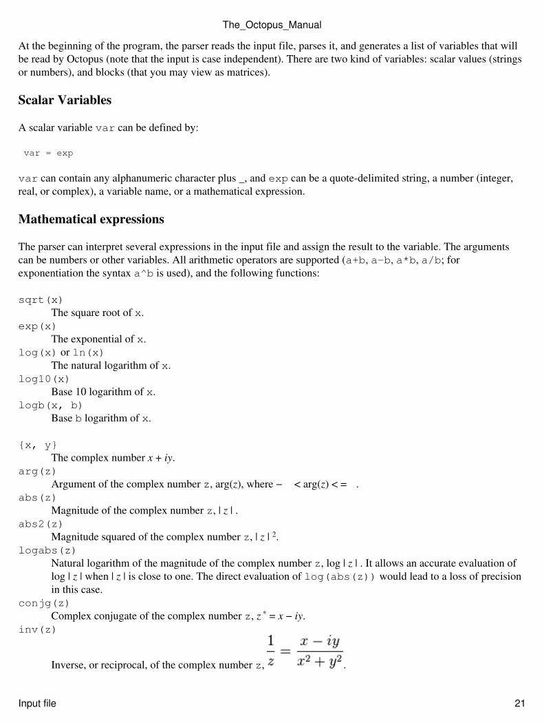
inv(z)
Inverse, or reciprocal, of the complex number z, .
The_Octopus_Manual
Input file 21
sin(x), cos(x), tan(x), cot(x), sec(x), csc(x)The sine, cosine, tangent, cotangent, secant and cosecant of x.
asin(x), acos(x), atan(x), acot(x), asec(x), acsc(x)The inverse (arc-) sine, cosine, tangent, cotangent, secant and cosecant of x.
atan2(x,y)= atan(y / x).
sinh(x), cosh(x), tanh(x), coth(x), sech(x), csch(x)The hyperbolic sine, cosine, tangent, cotangent, secant and cosecant of x.
asinh(x), acosh(x), atanh(x), acoth(x), asech(x), acsch(x)The inverse hyperbolic sine, cosine, tangent, cotangent, secant and cosecant of x.
min(x, y)The minimum of x and y.
max(x, y)The maximum of x and y.
step(x)The Heaviside step function in x. This can be used for piecewise-defined functions.
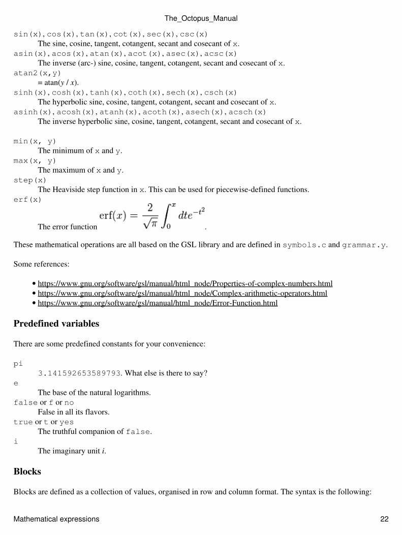
erf(x)
The error function .
These mathematical operations are all based on the GSL library and are defined in symbols.c and grammar.y.
Some references:
https://www.gnu.org/software/gsl/manual/html_node/Properties-of-complex-numbers.html• https://www.gnu.org/software/gsl/manual/html_node/Complex-arithmetic-operators.html• https://www.gnu.org/software/gsl/manual/html_node/Error-Function.html•
Predefined variables
There are some predefined constants for your convenience:
pi3.141592653589793. What else is there to say?
eThe base of the natural logarithms.
false or f or noFalse in all its flavors.
true or t or yesThe truthful companion of false.
iThe imaginary unit i.
Blocks
Blocks are defined as a collection of values, organised in row and column format. The syntax is the following:
The_Octopus_Manual
Mathematical expressions 22
%var exp | exp | exp | ... exp | exp | exp | ... ...%
Rows in a block are separated by a newline, while columns are separated by the character | or by a tab. There maybe any number of lines and any number of columns in a block. Note also that each line can have a different numberof columns. Values in a block don't have to be of the same type.
Comments
Everything following the character # until the end of the line is considered a comment and is simply cast intooblivion.
Default values
If Octopus tries to read a variable that is not defined in the input file, it automatically assigns to it a default value(there are some cases where Octopus cannot find a sensible default value and it will stop with an error). Allvariables read (present or not in the input file) are output to the file status/out.oct. If you are not sure ofwhat the program is reading, just take a look at it.
We recommend you to keep the variables in the input file to a minimum: do not write a variable that will beassigned its default value. The default can change in newer versions of Octopus and old values might causeproblems. Besides that, your input files become difficult to read and understand.
Documentation
Each input variable has (or should have) its own documentation explaining what it does and the valid values it maytake. This documentation can be obtained online or it can also be accessed by the oct-help command.
Experimental features
Even in the stable releases of Octopus there are many features that are being developed and are not suitable forproduction runs. To protect users from inadvertly using these parts they are declared as Experimental.
When you try to use one of these experimental functionalities Octopus will stop with an error. If you want to use ityou need to set the variable ExperimentalFeatures to yes. Now Octopus will only emit a warning.
By setting ExperimentalFeatures to yes you will be allowed to use parts of the code that are not completeor not well tested and most likely produce wrong results. If you want to use them for production runs you shouldcontact the Octopus developers first.
Good practices
In order to ensure compatibility with newer versions of Octopus and avoid problems, keep in mind the followingrules of good practice when writing input files:
The_Octopus_Manual
Blocks 23
Although input variables that take an option as an input can also take a number, the number representationmakes the input file less readable and it is likely to change in the future. So avoid using numbers insteadof values. For example
•
Units = ev_angstrom
must always be used instead of
Units = 3
Do not include variables that are not required in the input file, especially declarations of values that arejust a copy of the default value. This makes the input file longer, less readable and, since defaults are likelyto change, it makes more probable that your input file will have problems with newer versions of Octopus.Instead rely on default values.
•
Avoid duplicating information in the input file. Use your own variables and themathematical-interpretation capabilities for that. For example, you should use:
•
m = 0.1c = 137.036E = m*c^2
instead of
m = 0.1c = 137.036E = 1877.8865
In the second case, you might change the value of m (or c if you are a cosmologist) while forgetting to update E,ending up with an inconsistent file.
Previous Manual:Installation - Next Manual:Running Octopus
Back to Manual <p class=newpage>
Running Octopus
Input
In order to run, Octopus requires an input file that must be called inp. Depending on your input file there are otherfiles that you might need, like pseudopotentials or coordinate files (we will discuss this later in this manual).
The rest of the files that are required are part of the Octopus installation; if Octopus is correctly installed theyshould be available and Octopus should know where to find them. With Octopus you can't just copy the binarybetween systems and expect it to work.
The_Octopus_Manual
Good practices 24
Executing
To run Octopus you just have to give the octopus command in the directory where you have your input file.While running, octopus will display information on the screen. If you want to capture this information you cansend the output to a file, let's say out.log, by executing it like this:
$ octopus > out.log
This captures only the normal output. If there is a warning or an error, it will be still printed on the screen. Tocapture everything to a file, run
$ octopus >& out.log
If you want to run Octopus in the background, append & to the last command.
Output
While running, Octopus will create several output files, all of them inside subdirectories in the same directorywhere it was run. The files that contain the physical information depend on what Octopus is doing and they will bediscussed in the next chapter.
One directory that is always created is exec/, this file contains information about the Octopus run. Here you willfind the oct.out file, a text file that contains all the input variables that were read by Octopus, both the variablesthat are in the input file and the variables that took default values; in the second case they are marked by acomment as #default. This file is very useful if you want to check that octopus is correctly parsing a variable orwhat are the default values that it is taking.
Clean Stop
If you create a file called stop in the running directory, Octopus will exit gracefully after finishing the currentiteration. May not work for gcm, invert_ks, casida, td_transport, one_shot run modes. You can use this to preventpossible corruption of restart information when your job is killed by a scheduler, by preemptively asking Octopusto quit automatically in a job script like this:
#PBS -l walltime=4:10:00mpirun $HOME/octopus/bin/octopus_mpi &> output &sleep 4htouch stopwait
or more sophisticatedly like this:
MIN=`qstat -a $PBS_JOBID | awk '{wall=$9} END {print $9}' | awk -F: '{min=($1*60)+$2; print min}'`sh ~/sleep_stop.sh stop $((MIN-10))m > sleepy &mpirun $HOME/octopus/bin/octopus_mpi &> output
with auxiliary script sleep_stop.sh:
#!/bin/bashif [ $# -ne 2 ]; then
The_Octopus_Manual
Executing 25
echo "Usage: sleep_stop.sh FILENAME TIME"else echo "Time until $1 created: $2" rm -f $1 sleep $2 touch $1fi
Restarting
Another directory that will created is restart/; in this directory Octopus saves the information from thecalculation that it is doing. This information can be used in the following cases:
If Octopus is stopped without finishing by some reason, it can restart from where it was without having todo all work again.
•
If after the calculation is done (or even if it was stopped), the user wants to do the same simulation withsome different parameters, Octopus can save some work by starting from the restart information.
•
There are some calculations that require the results of other type of calculation as an input; in this case ituses the files written in restart/ by the previous calculation (we will discuss this case later, when wetalk about the different calculation modes).
•
Sometimes it's not desired to restart a calculation, but to start it from the very beginning. Octopus can be instructedto do so by setting the input variable fromScratch to yes.
Previous Manual:Input file - Next Manual:Units
Back to Manual <p class=newpage>
Units
Before entering into the physics in Octopus we have to address a very important issue: units. There are differentunit systems that can be used at the atomic scale: the most used are atomic units and what we call "convenient"units. Here we present both unit systems and explain how to use them in Octopus.
Atomic Units
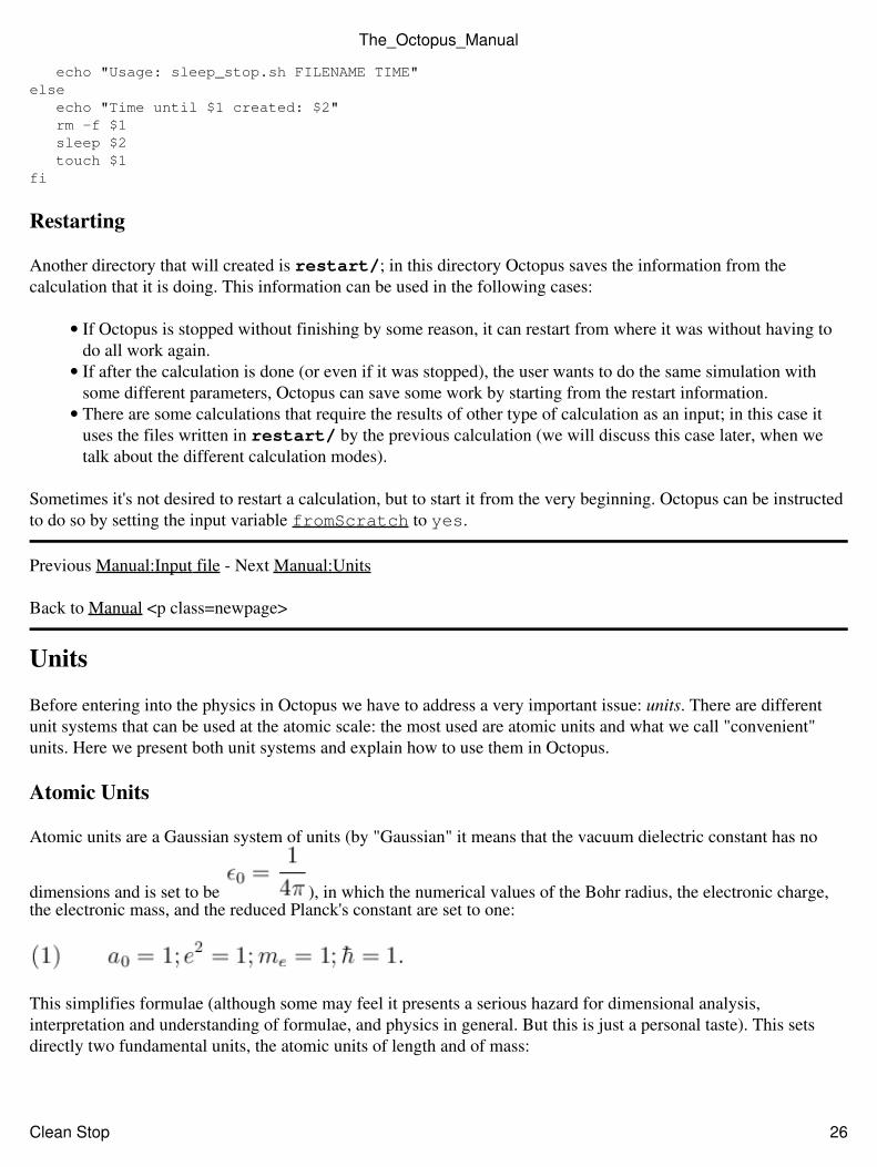
Atomic units are a Gaussian system of units (by "Gaussian" it means that the vacuum dielectric constant has no
dimensions and is set to be ), in which the numerical values of the Bohr radius, the electronic charge,the electronic mass, and the reduced Planck's constant are set to one:
This simplifies formulae (although some may feel it presents a serious hazard for dimensional analysis,interpretation and understanding of formulae, and physics in general. But this is just a personal taste). This setsdirectly two fundamental units, the atomic units of length and of mass:
The_Octopus_Manual
Clean Stop 26
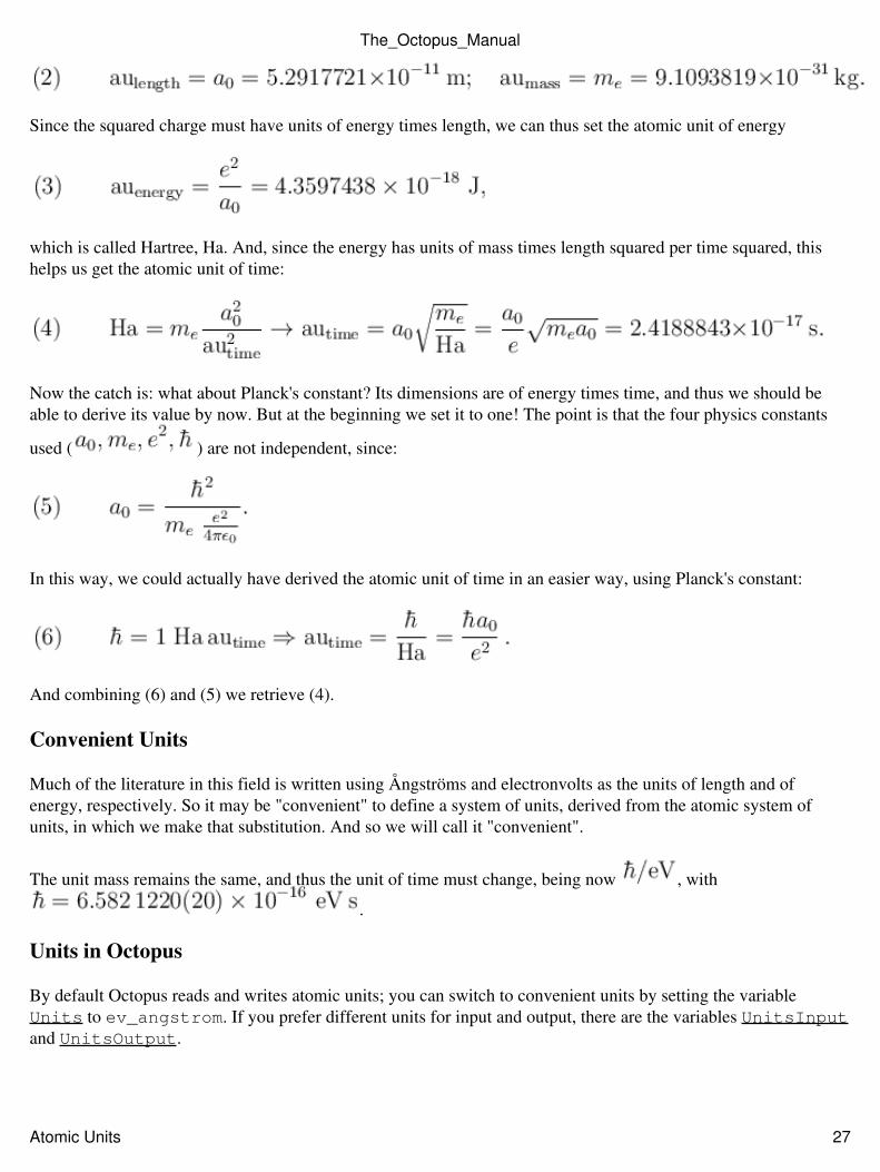
Since the squared charge must have units of energy times length, we can thus set the atomic unit of energy
which is called Hartree, Ha. And, since the energy has units of mass times length squared per time squared, thishelps us get the atomic unit of time:
Now the catch is: what about Planck's constant? Its dimensions are of energy times time, and thus we should beable to derive its value by now. But at the beginning we set it to one! The point is that the four physics constants
used ( ) are not independent, since:
In this way, we could actually have derived the atomic unit of time in an easier way, using Planck's constant:
And combining (6) and (5) we retrieve (4).
Convenient Units
Much of the literature in this field is written using Ångströms and electronvolts as the units of length and ofenergy, respectively. So it may be "convenient" to define a system of units, derived from the atomic system ofunits, in which we make that substitution. And so we will call it "convenient".
The unit mass remains the same, and thus the unit of time must change, being now , with
.
Units in Octopus
By default Octopus reads and writes atomic units; you can switch to convenient units by setting the variableUnits to ev_angstrom. If you prefer different units for input and output, there are the variables UnitsInputand UnitsOutput.
The_Octopus_Manual
Atomic Units 27
Mass Units
An exception for units in Octopus is mass units. When dealing with the mass of ions, always atomic mass units(amu) are used. This unit is defined as 1 / 12 of the mass of the 12C atom. In keeping with standard conventions insolid-state physics, effective masses of electrons are always reported in units of the electron mass (i.e. the atomicunit of mass), even in the eV-Å system.
Charge Units
In both unit systems, the charge unit is the electron charge e (i.e. the atomic unit of charge).
Unit Conversions
Converting units can be a very time-consuming and error-prone task when done by hand, especially when there areimplicit constants set to one, as in the case of atomic units. That is why it's better to use as specialized software likeGnu Units.
In some fields, a very common unit to express the absorption spectrum is Mb. To convert a strength function from
1/eV to Mb, multiply by , with . The numerical factor is 109.7609735.
Previous Manual:Running Octopus - Next Manual:Physical System
Back to Manual <p class=newpage>
Physical System
The first thing that octopus has to know is the physical system you want to treat. To do this you have specify agroup of species and their positions.
Dimensions
Octopus can work in a space with 1, 2 or 3 dimensions. You can select the dimension of your system with theDimensions variable.
Species
An Octopus species is very generic and can be a nucleus (represented by pseudopotentials or by the full Coulombpotential), a jellium sphere or even a user-defined potential. The information regarding the atomic species goes intothe Species block.
Pseudopotentials
The many-electron Schroedinger equation can be greatly simpli?ed if electrons are divided in two groups: valenceelectrons and inner core electrons. The electrons in the inner shells are strongly bound and do not play a signi?cant
The_Octopus_Manual
Mass Units 28
role in the chemical binding of atoms, thus forming with the nucleus an inert core. Binding properties are almostcompletely due to the valence electrons, especially in metals and semiconductors. This separation implies thatinner electrons can be ignored, reducing the atom to an inert ionic core that interacts with the valence electrons.This suggests the use of an e?ective interaction, a pseudopotential, that gives an approximation to the potential feltby the valence electrons due to the nucleus and the core electrons. This can signi?cantly reduce the number ofelectrons that have to be dealt with. Moreover, the pseudo wave functions of these valence electrons are muchsmoother in the core region than the true valence wave functions, thus reducing the computational burden of thecalculations.
Modern pseudopotentials are obtained by inverting the free atom Schroedinger equation for a given referenceelectronic con?guration, and forcing the pseudo wave functions to coincide with the true valence wave functionsbeyond a certain cuto? distance. The pseudo wave functions are also forced to have the same norm as the truevalence wave functions, and the energy pseudo eigenvalues are matched to the true valence eigenvalues. Di?erentmethods of obtaining a pseudo eigenfunction that satis?es all these requirements lead to di?erent non-local, angularmomentum dependent pseudopotentials. Some widely used pseudopotentials are the Troullier and Martins [9]potentials, the Hamann [10] potentials, the Vanderbilt [11] potentials and the Hartwigsen-Goedecker-Hutter [12]potentials. The default potentials used by octopus are of the Troullier and Martins type, although you can also optfor the HGH potentials.
Octopus comes with a package of pseudopotentials and the parameters needed to use them. If you want to have alook you can find them under PREFIX/share/octopus/PP. These pseudopotentials serve to define manyspecies that you might wish to use in your coordinates block, e.g. a helium atom, "He". If you are happy to usethese predefined pseudopotentials, you do not need to write a species block.
However it is also possible to define new species to use in your coordinates block by adding a Species block.You can check the documentation of that variable for the specific syntax. With this block you may specify theformat of your file that contains a pseudopotential and parameters such as the atomic number, or you may definean algebraic expression for the potential with the user-defined potential. A user defined potential should be finiteeverywhere in the region where your calculation runs.
If you want to create other pseudopotentials, you can do it in the pseudopotentials generator. Save the file in thesame directory as the inp file and specify the format of the file with the species block.
All-Electron Nucleus
The potential of this species is the full Coulomb potential
The main problem to represent this potential is the discontinuity over . To overcome this problem we do thefollowing:
First we assume that atoms are located over the closest grid point.• Then we calculate the charge density associated with the nucleus: a delta distribution with the value of thecharge at this point and zero elsewhere.
•
Now we solve the Poisson equation for this density.•
The_Octopus_Manual
Pseudopotentials 29
In this way we get a potential that is the best representation of the Coulomb potential for our grid (we will discuss
about grids later) and is continuous in (the value is the average of the potential over the volume associatedwith the grid point).
The main problem is that the requirement of having atoms over grid points is quite strong: it is only possible for afew systems with simple geometries and you can't move the atoms. Also the Coulomb potential is very hard, whichmeans you will need a very small spacing, and as you have to consider both core and valence electrons, this speciesis only suitable for atoms or very small molecules.
User Defined
It is also possible to define an external, user-defined potential in the input file. All functions accepted by the parsercan be used. Besides that, one can use the symbols x, y, z, and r. In this way it is trivial to calculate model systems,like harmonic oscillators, quantum dots, etc.
Coordinates
For each instance of a species (even for user-defined potentials), you have to specify its position inside thesimulation box. To do this you can use Coordinates block which describes the positions inside of the input fileor one of the XYZCoordinates or PDBCoordinates variables, that specify an external file, in xyz or PDBformat respectively, from where the coordinates will be read.
Before using a geometry with octopus you have to center it, for this you can use the oct-center-geom utility.
Velocities
If you are going to do ion dynamics you may want to have an initial velocity for the particles. You have severalchoices for doing this:
Don't put anything in the input file; particles will have zero initial velocity.• Give them a random velocity according to a temperature (in degrees Kelvin) given by theRandomVelocityTemp variable.
•
Explicitly give the initial velocity for each particle, either through the Velocities block or from apseudo-xyz file detailed by the variable XYZVelocities.
•
Number of Electrons
Each species adds enough electrons to make the system neutral. If you want to add or remove electrons you canspecify the total charge of your system with the ExcessCharge variable (a negative charge implies to addelectrons).
Previous Manual:Units - Next Manual:Hamiltonian
Back to Manual <p class=newpage>
The_Octopus_Manual
All-Electron Nucleus 30
Hamiltonian
Octopus is based upon Density Functional Theory in the Kohn-Sham formulation. The Kohn-Sham Hamiltonian isthe main part of this formulation; in this section we describe how the Hamiltonian is treated in octopus and whatare the variables that control it.
Introduction
Although the Hohenberg-Kohn theorem states that DFT is exact, the Kohn-Sham method of reducing aninteracting many-particle problem to a non-interacting single-particle problem introduces an approximation: theexchange-correlation term.
Ground-State DFT
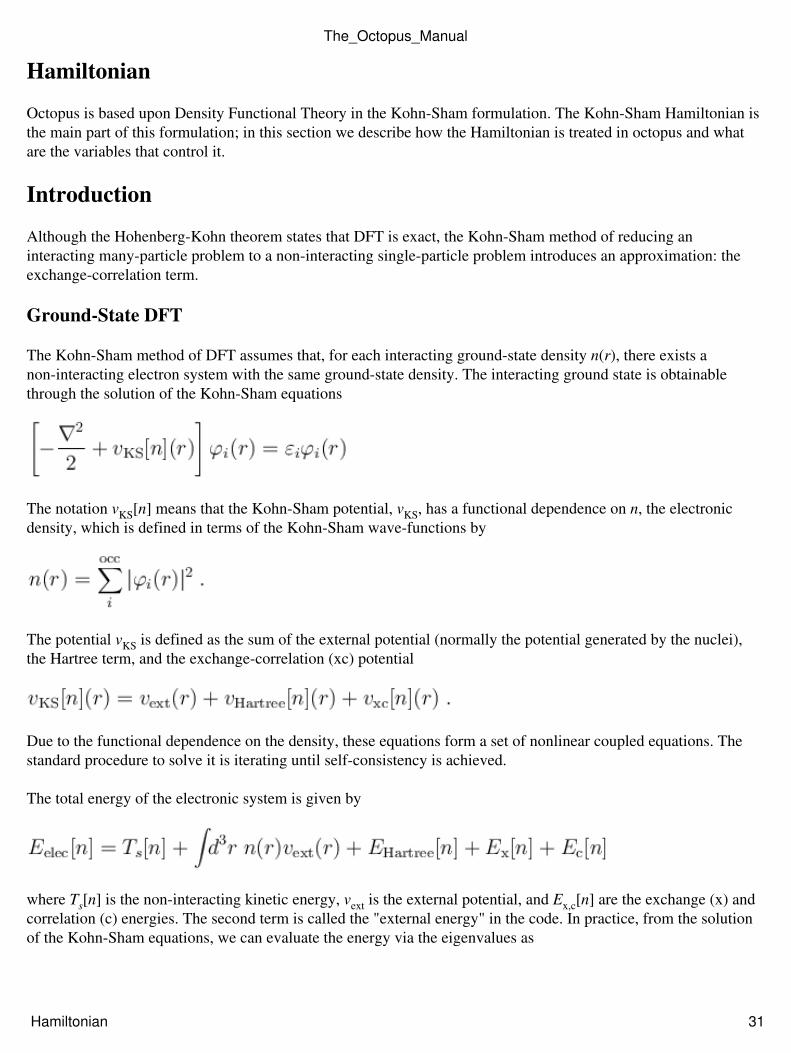
The Kohn-Sham method of DFT assumes that, for each interacting ground-state density n(r), there exists anon-interacting electron system with the same ground-state density. The interacting ground state is obtainablethrough the solution of the Kohn-Sham equations
The notation vKS[n] means that the Kohn-Sham potential, vKS, has a functional dependence on n, the electronicdensity, which is defined in terms of the Kohn-Sham wave-functions by
The potential vKS is defined as the sum of the external potential (normally the potential generated by the nuclei),the Hartree term, and the exchange-correlation (xc) potential
Due to the functional dependence on the density, these equations form a set of nonlinear coupled equations. Thestandard procedure to solve it is iterating until self-consistency is achieved.
The total energy of the electronic system is given by
where Ts[n] is the non-interacting kinetic energy, vext is the external potential, and Ex,c[n] are the exchange (x) andcorrelation (c) energies. The second term is called the "external energy" in the code. In practice, from the solutionof the Kohn-Sham equations, we can evaluate the energy via the eigenvalues as
The_Octopus_Manual
Hamiltonian 31
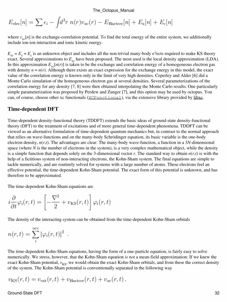
where vxc[n] is the exchange-correlation potential. To find the total energy of the entire system, we additionallyinclude ion-ion interaction and ionic kinetic energy.
Exc = Ex + Ec is an unknown object and includes all the non-trivial many-body e?ects required to make KS theoryexact. Several approximations to Exc have been proposed. The most used is the local density approximation (LDA).In this approximation Exc[n(r)] is taken to be the exchange and correlation energy of a homogeneous electron gaswith density n = n(r). Although there exists an exact expression for the exchange energy in this model, the exactvalue of the correlation energy is known only in the limit of very high densities. Ceperley and Alder [6] did aMonte Carlo simulation of the homogeneous electron gas at several densities. Several parameterizations of thecorrelation energy for any density [7, 8] were then obtained interpolating the Monte Carlo results. One particularlysimple parameterization was proposed by Perdew and Zunger [7], and this option may be used by octopus. Youcan, of course, choose other xc functionals (XCFunctional), via the extensive library provided by libxc.
Time-dependent DFT
Time-dependent density-functional theory (TDDFT) extends the basic ideas of ground-state density-functionaltheory (DFT) to the treatment of excitations and of more general time-dependent phenomena. TDDFT can beviewed as an alternative formulation of time-dependent quantum mechanics but, in contrast to the normal approachthat relies on wave-functions and on the many-body Schrödinger equation, its basic variable is the one-bodyelectron density, n(r,t). The advantages are clear: The many-body wave-function, a function in a 3N-dimensionalspace (where N is the number of electrons in the system), is a very complex mathematical object, while the densityis a simple function that depends solely on the 3-dimensional vector r. The standard way to obtain n(r,t) is with thehelp of a fictitious system of non-interacting electrons, the Kohn-Sham system. The final equations are simple totackle numerically, and are routinely solved for systems with a large number of atoms. These electrons feel aneffective potential, the time-dependent Kohn-Sham potential. The exact form of this potential is unknown, and hastherefore to be approximated.
The time-dependent Kohn-Sham equations are
The density of the interacting system can be obtained from the time-dependent Kohn-Sham orbitals
The time-dependent Kohn-Sham equations, having the form of a one-particle equation, is fairly easy to solvenumerically. We stress, however, that the Kohn-Sham equation is not a mean-field approximation: If we knew theexact Kohn-Sham potential, vKS, we would obtain the exact Kohn-Sham orbitals, and from these the correct densityof the system. The Kohn-Sham potential is conventionally separated in the following way
The_Octopus_Manual
Ground-State DFT 32
The first term is again the external potential. The Hartree potential accounts for the classical electrostaticinteraction between the electrons
The time-dependence of the exchange and correlation potential introduces the need for an approximation beyondthe one made in the time-independent case. The simplest method of obtaining a time-dependent xc potentialconsists in assuming that the potential is the time-independent xc potential evaluated at the time-dependent density,i.e.,
This is called the adiabatic approximation. If the time-independent xc potential chosen is the LDA, then we obtainthe so-called adiabatic local density approximation (ALDA). This approximation gives remarkably good excitationenergies but su?ers from the same problems as the LDA, most notably the exponential fall-o? of the xc potential. Ifa strong laser pushes the electrons to regions far from the nucleus, ALDA should not be expected to give anaccurate description of the system. Other options for the time-dependent xc potential are orbital-dependentpotentials like the exact exchange functional (EXX) (usually in the Krieger-Li-Iafrate (KLI) approximation).
Occupations
You can set the occupations the orbitals by hand, using the Occupations.
External Potential
You can add an external uniform and constant electric or magnetic field, set by the StaticElectricField orStaticMagneticField. If you want to add a more general potential, you can do it using a user-definedSpecies.
If you got the coordinates from a PDB file, you can add the potential generated by the point charges defined thereby setting the ClassicPotential variable to yes.
Electron-Electron Interaction
You can neglect this term by setting TheoryLevel = independent_particles variable. This impliesthat both the Hartree and exchange-correlation terms will not be calculated.
Exchange and correlation potential
Octopus does not distinguish, for the moment, between ground-state DFT xc functionals, and time-dependent DFTfunctionals. In other words, in all cases the adiabatic approximation is assumed. In mathematical terms, we mayformalize this in the following way: let n be the time-dependent density, a function living in the four-dimensional
space-time world. We will call , the electronic density at time , a function in thethree-dimensional space. An exchange and/or correlation energy functional in ground state DFT may then be
The_Octopus_Manual
Time-dependent DFT 33
used to build an adiabatic exchange and/or correlation action functional in the following way:
The time-dependent potential functional is then:
We use the distinct notation and to stress that the exchange and correlationpotential in TDDFT -- the former -- and the exchange and correlation potential in GS-DFT -- the latter -- are inprinciple two conceptually different objects, which coincide only thanks to the adiabatic approximation. This is thereason why we may actually only refer to the functionals in the GS-DFT context.
We may classify the xc functionals contained in the Octopus code following John Perdew's Jacob's Ladder scheme:
LDA rung: A functional belonging to the LDA rung depends only on the electronic density (on the spindensity in spin-polarized or spinors cases). Moreover, it has a local dependency on the density, i.e.:
•
The potential may be then derived by functional derivation:
GGA rung: A functional belonging to the GGA rung depends on the electronic density, and also on itsgradient. Moreover, it also has a local dependency (actually, the GGA is very often called a semi-localfunctional due to this).
•
meta-GGA rung:•
OEP rung: This is the family of functionals which are defined in terms of the occupied Kohn-Sham orbitals,
. These are in fact the only non-local functionals. The name of the rung, OEP, stands for"optimized-effective-potential", the reason being that in general this is the method used to derive thepotential from the energy functional (direct functional derivation is in this case not possible). A moresuitable name would be orbital-dependent functionals.
•
Octopus comes with several Exchange and Correlation potentials, including several flavours of LDA, GGA and
The_Octopus_Manual
Exchange and correlation potential 34
OEP. You can choose your favorites by setting the variable XCFunctional. (Note that until Octopus <= 2.1 theexchange-correlation functional was chosen with the variables XFunctional and CFunctional.)
When using OEP Exchange, the variable OEP_level controls the level of approximation required.
You can also include Self-Interaction Correction (SIC), controlled by the variable SICCorrection.
Relativistic Corrections
The variable RelativisticCorrection allows one to choose the relativistic correction to be used. Up tonow only spin-orbit coupling (RelativisticCorrection = spin_orbit) is implemented.
Spin-orbit Coupling
The spin-orbit coupling as it is implemented in octopus is included in the pseudo-potentials. These can either beHGH pseudo-potentials or Troullier-Martins-like pseudo-potentials. In the later case the pseudo-potentials need tobe generated from fully relativistic calculations and their fully separable form is given by:
Since the angular part of the pseudo wave-functions are spherical spinors the wave-functions should becomplex spinors and so the SpinComponents needs to be set to non_collinear. This is also true for HGHpseudo-potentials.
Note that currently octopus is only able to read j-dependent Troullier-Martins-like pseudo-potentials that areprovided in the UPF file format.
Previous Manual:Physical System - Next Manual:Discretization
Back to Manual <p class=newpage>
Discretization
Besides all the approximations we have to do, no computer can solve an infinite continuous problem. We have todiscretize our equations somehow. Octopus uses a grid in real space to solve the Kohn-Sham equations. That is,functions are represented by their value over a set of points in real space. Normally the grid is equally spaced, butalso non-uniform grids can be used. The shape of the simulation region may also be tuned to suit the geometricconfiguration of the system.
The_Octopus_Manual
Relativistic Corrections 35
Grid
In Octopus functions are represented by a set of values that correspond to the value of the function over a set ofpoints in real space. By default these points are distributed in a uniform grid, which means that the distancebetween points is a constant for each direction. It is possible to have grids that are not uniform, but as this is a bitmore complex we will discuss it later.
In this scheme, the separation between points, or spacing, is a critical value. When it becomes large therepresentation of functions gets worse and when it becomes small the number of points increases, increasingmemory use and calculation time. This value is equivalent to the energy cutoff used by plane-wave representations.
In Octopus you can choose the Spacing of your simulation by the Spacing variable. If you set this as a singlevalue it will give the same spacing for each directions (for example Spacing=0.3). If you want to have differentspacings for each coordinate you can specify Spacing as a block of three real values.
If you are working with the default pseudopotential species of Octopus they come with a recommended Spacingvalue and you don't need to give it in the input file. Normally this default values are around 0.4 [b] (~0.2 [Å]), butyou may need smaller spacing in some cases. Do not rely on these default values for production runs.
Double grid (experimental)
The double-grid technique is a method to increase the precision of the representation of the pseudopotentials in thegrid that has been recently integrated in Octopus (not available in Octopus 2.1 and previous versions). To activatethis technique, set the variable DoubleGrid to yes. The use of a double grid increases the cost of the transfer ofthe potential to the grid, but as in most cases this is done only a few times per run, the overhead to the totalcomputation time is negligible. The only exception is when the atoms are displaced while doing a time-dependentsimulation, where the double grid can severely increase the computation time.
Box
We also have to select a finite domain of the real space to run our simulation, which is known as the simulationbox. Octopus can use several kinds of shapes of box. This is controlled by the variable BoxShape. Besidesstandard shapes Octopus can take shapes given by a user-defined function or even by an image.
The way to give the size of the simulation box changes for each shape, but for most of them it is given by thevariable Radius.
Zero boundary conditions
By default Octopus assumes zero boundary conditions, that is, wavefunctions and density are zero over theboundary of the domain. This is the natural boundary condition when working with finite systems.
In this case choosing an adequate box size is very important: if the box is too small the wavefunctions will beforced to go to zero unnaturally, but if the box is too large, a larger number of points is needed, increasingcalculation time and memory requirements.
Previous Manual:Hamiltonian - Next Manual:Output
The_Octopus_Manual
Grid 36
Back to Manual <p class=newpage>
Output
At first you may be quite happy that you have mastered the input file, and octopus runs without errors. However,eventually you (or your thesis advisor) will want to learn something about the system you have managed todescribe to Octopus.
Ground-State DFT
Octopus sends some relevant information to the standard output (which you may have redirected to a file). Hereyou will see energies and occupations of the eigenstates of your system. These values and other information canalso be found in the file static/info.
However Octopus also calculates the wavefunctions of these states and the positions of the nuclei in your system.Thus it can tell you the density of the dipole moment, the charge density, or the matrix elements of the dipolemoment operator between different states. Look at the values that the Output variable can take to see thepossibilities.
For example, if you include
Output = wfs_sqmod + potential
in your inp file, Octopus will create separate text files in the directory static with the values of the squaremodulus of the wave function and the local, classical, Hartree, and exchange/correlation parts of the Kohn-Shampotential at the points in your mesh.
You can specify the formatting details for these input files with the OutputHow variable and the other variablesin the Output section of the Reference Manual. For example, you can specify that the file will only containvalues along the x, y, or z axis, or in the plane x=0, y=0, or z=0. You can also set the format to be readable by thegraphics programs OpenDX, gnuplot or MatLab. OpenDX can make plots of iso-surfaces if you have data inthree-dimensions. However gnuplot can only make a 3-d plot of a function of two variables, i.e. if you have thevalues of a wavefunction in a plane, and 2-d plots of a function of one variable, i.e. the value of the wavefunctionalong an axis.
Time-Dependent DFT
Optical Properties
A primary reason for using a time-dependent DFT program is to obtain the optical properties of your system. Youhave two choices for this, linear-response theory a la Jamorski, Casida & Salahub [1], or explicit time-propagationof the system after a perturbation, a la Yabana & Bertsch [2]. You may wish to read more about these methods inthe paper by Castro et al.[3]
Linear-Response Theory
Linear-response theory is based on the idea that a small (time-dependent) perturbation in an externally appliedelectric potential δv(r,ω) will result in a (time-dependent) perturbation of the electronic density δρ(r,ω) which is
The_Octopus_Manual
Zero boundary conditions 37
linearly related to the size of the perturbation: . Here, obviously,the time-dependence is Fourier-transformed into a frequency-dependence, ω. The susceptibility, χ(r,r';ω), is adensity-density response function, because it is the response of the charge density to a potential that couples to thecharge density of the system. Because of this, it has poles at the excitation energies of the many-body system,meaning that the induced density also has these poles. One can use this analytical property to find a relatedoperator whose eigenvalues are these many-body excitation energies. The matrix elements of the operator containamong other things: 1) occupied and unoccupied Kohn-Sham states and energies (from a ground state DFT
calculation) and 2) an exchange-correlation kernel, .
Casida's equations are a full solution to this problem (for real wavefunctions). The Tamm-Dancoff approximationuses only occupied-unoccupied transitions. The Petersilka approximation uses only the diagonal elements of theTamm-Dancoff matrix, i.e. there is no mixing of transitions.[4]It takes only a little more time to calculate the wholematrix, so Petersilka is provided mostly for comparison.
These methods are clearly much faster (an order of magnitude) than propagating in time, but it turns out that theyare very sensitive to the quality of the unoccupied states. This means that it is very hard to converge the excitationenergy, because one requires a very large simulation box (much larger than when propagating in real time).
Electronic Excitations by Means of Time-Propagation
See Manual:Time_Dependent#Delta_kick:_Calculating_an_absorption_spectrum.
References
? Christine Jamorski, Mark E. Casida, and Dennis R. Salahub, Dynamic polarizabilities and excitationspectra from a molecular implementation of time-dependent density-functional response theory: N2 as acase study, J. Chem. Phys. 5134-5147 (1996)
1.
? K. Yabana, G. F. Bertsch, Time-dependent local-density approximation in real time, Phys. Rev. B 4484 -4487 (1996)
2.
? Alberto Castro, Heiko Appel, Micael Oliveira, Carlo A. Rozzi, Xavier Andrade, Florian Lorenzen, M. A.L. Marques, E. K. U. Gross, Angel Rubio, octopus: a tool for the application of time-dependent densityfunctional theory, physica status solidi (b) 243 2465-2488 (2006)
3.
? Petersilka, M. and Gossmann, U. J. and Gross, E. K. U., Excitation Energies from Time-DependentDensity-Functional Theory, Phys. Rev. Lett. 76 1212--1215 (1996)
4.
Previous Manual:Discretization - Next Manual:Troubleshooting
Back to Manual <p class=newpage>
The_Octopus_Manual
Linear-Response Theory 38
Troubleshooting
If Octopus works properly on your system (i.e. you can recreate the results in the tutorial) but you have troublesusing it for your own work, here are some things to try. Please feel free to add your own ideas here.
Read parser.log
If you look at the file exec/parser.log, it will tell you the value of the variables that you set with the inpfile, as well as all the variables which are taking their default value. This can sometimes be helpful inunderstanding the behavior of the program.
Use OutputDuringSCF
If you add OutputDuringSCF = yes to your input file, you can examine the results of each iteration in the SelfConsistent Field calculation. So if you also have the variable Output set to Output = density +potential, both the electron density and the Kohn-Sham, bare, exchange-correlation and Hartree potentials willbe written to a folder (called, e.g., scf.0001) after each SCF iteration.
Set DebugLevel
Set the variable DebugLevel to 1 for some extra diagnostic info and a stack trace with any fatal error, 2 to add afull stack strace, and 99 to get a stack trace from each MPI task when running in parallel.
Previous Manual:Output - Next Manual:Symmetry
Back to Manual <p class=newpage>
Symmetry
There is not much use of symmetry in Octopus.
In finite systems, you will get an analysis just for your information, but which will not be used anywhere in thecode. It is of this form (e.g. for silane):
***************************** Symmetries *****************************Symmetry elements : 4*(C3) 3*(C2) 3*(S4) 6*(sigma)Symmetry group : Td**********************************************************************
Many symmetries will in fact be broken by the real-space mesh. Since it is always orthogonal, it will breakthree-fold rotational symmetry of benzene, for example.
In periodic systems, you will also get an analysis, e.g like this for bulk silicon in its 8-atom convention cell:
***************************** Symmetries *****************************Space group No.227 International: Fd -3 m International(long): Fd -3 m _1 Schoenflies: Oh^7
The_Octopus_Manual
Troubleshooting 39
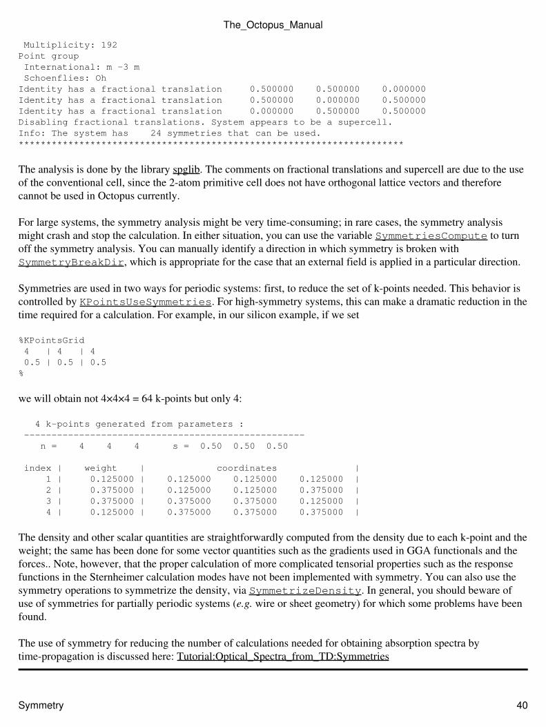
Multiplicity: 192Point group International: m -3 m Schoenflies: OhIdentity has a fractional translation 0.500000 0.500000 0.000000Identity has a fractional translation 0.500000 0.000000 0.500000Identity has a fractional translation 0.000000 0.500000 0.500000Disabling fractional translations. System appears to be a supercell.Info: The system has 24 symmetries that can be used.**********************************************************************
The analysis is done by the library spglib. The comments on fractional translations and supercell are due to the useof the conventional cell, since the 2-atom primitive cell does not have orthogonal lattice vectors and thereforecannot be used in Octopus currently.
For large systems, the symmetry analysis might be very time-consuming; in rare cases, the symmetry analysismight crash and stop the calculation. In either situation, you can use the variable SymmetriesCompute to turnoff the symmetry analysis. You can manually identify a direction in which symmetry is broken withSymmetryBreakDir, which is appropriate for the case that an external field is applied in a particular direction.
Symmetries are used in two ways for periodic systems: first, to reduce the set of k-points needed. This behavior iscontrolled by KPointsUseSymmetries. For high-symmetry systems, this can make a dramatic reduction in thetime required for a calculation. For example, in our silicon example, if we set
%KPointsGrid 4 | 4 | 4 0.5 | 0.5 | 0.5%
we will obtain not 4×4×4 = 64 k-points but only 4:
4 k-points generated from parameters : --------------------------------------------------- n = 4 4 4 s = 0.50 0.50 0.50
index | weight | coordinates | 1 | 0.125000 | 0.125000 0.125000 0.125000 | 2 | 0.375000 | 0.125000 0.125000 0.375000 | 3 | 0.375000 | 0.375000 0.375000 0.125000 | 4 | 0.125000 | 0.375000 0.375000 0.375000 |
The density and other scalar quantities are straightforwardly computed from the density due to each k-point and theweight; the same has been done for some vector quantities such as the gradients used in GGA functionals and theforces.. Note, however, that the proper calculation of more complicated tensorial properties such as the responsefunctions in the Sternheimer calculation modes have not been implemented with symmetry. You can also use thesymmetry operations to symmetrize the density, via SymmetrizeDensity. In general, you should beware ofuse of symmetries for partially periodic systems (e.g. wire or sheet geometry) for which some problems have beenfound.
The use of symmetry for reducing the number of calculations needed for obtaining absorption spectra bytime-propagation is discussed here: Tutorial:Optical_Spectra_from_TD:Symmetries
The_Octopus_Manual
Symmetry 40
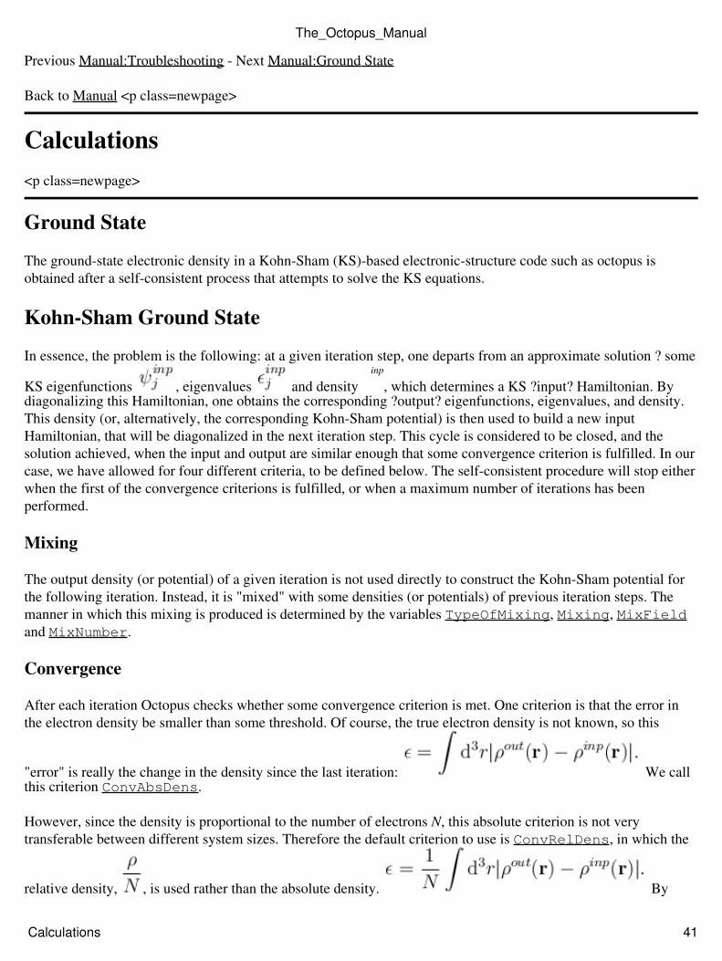
Previous Manual:Troubleshooting - Next Manual:Ground State
Back to Manual <p class=newpage>
Calculations<p class=newpage>
Ground State
The ground-state electronic density in a Kohn-Sham (KS)-based electronic-structure code such as octopus isobtained after a self-consistent process that attempts to solve the KS equations.
Kohn-Sham Ground State
In essence, the problem is the following: at a given iteration step, one departs from an approximate solution ? some
KS eigenfunctions , eigenvalues and density ρinp
, which determines a KS ?input? Hamiltonian. Bydiagonalizing this Hamiltonian, one obtains the corresponding ?output? eigenfunctions, eigenvalues, and density.This density (or, alternatively, the corresponding Kohn-Sham potential) is then used to build a new inputHamiltonian, that will be diagonalized in the next iteration step. This cycle is considered to be closed, and thesolution achieved, when the input and output are similar enough that some convergence criterion is fulfilled. In ourcase, we have allowed for four different criteria, to be defined below. The self-consistent procedure will stop eitherwhen the first of the convergence criterions is fulfilled, or when a maximum number of iterations has beenperformed.
Mixing
The output density (or potential) of a given iteration is not used directly to construct the Kohn-Sham potential forthe following iteration. Instead, it is "mixed" with some densities (or potentials) of previous iteration steps. Themanner in which this mixing is produced is determined by the variables TypeOfMixing, Mixing, MixFieldand MixNumber.
Convergence
After each iteration Octopus checks whether some convergence criterion is met. One criterion is that the error inthe electron density be smaller than some threshold. Of course, the true electron density is not known, so this
"error" is really the change in the density since the last iteration: We callthis criterion ConvAbsDens.
However, since the density is proportional to the number of electrons N, this absolute criterion is not verytransferable between different system sizes. Therefore the default criterion to use is ConvRelDens, in which the
relative density, , is used rather than the absolute density. By
The_Octopus_Manual
Calculations 41
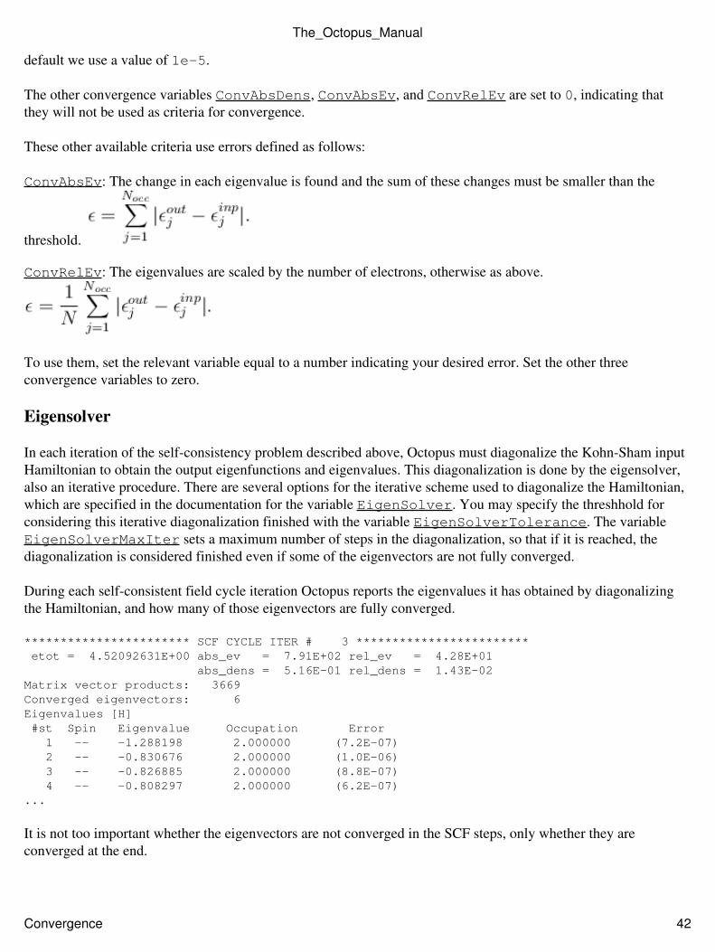
default we use a value of 1e-5.
The other convergence variables ConvAbsDens, ConvAbsEv, and ConvRelEv are set to 0, indicating thatthey will not be used as criteria for convergence.
These other available criteria use errors defined as follows:
ConvAbsEv: The change in each eigenvalue is found and the sum of these changes must be smaller than the
threshold.
ConvRelEv: The eigenvalues are scaled by the number of electrons, otherwise as above.
To use them, set the relevant variable equal to a number indicating your desired error. Set the other threeconvergence variables to zero.
Eigensolver
In each iteration of the self-consistency problem described above, Octopus must diagonalize the Kohn-Sham inputHamiltonian to obtain the output eigenfunctions and eigenvalues. This diagonalization is done by the eigensolver,also an iterative procedure. There are several options for the iterative scheme used to diagonalize the Hamiltonian,which are specified in the documentation for the variable EigenSolver. You may specify the threshhold forconsidering this iterative diagonalization finished with the variable EigenSolverTolerance. The variableEigenSolverMaxIter sets a maximum number of steps in the diagonalization, so that if it is reached, thediagonalization is considered finished even if some of the eigenvectors are not fully converged.
During each self-consistent field cycle iteration Octopus reports the eigenvalues it has obtained by diagonalizingthe Hamiltonian, and how many of those eigenvectors are fully converged.
*********************** SCF CYCLE ITER # 3 ************************ etot = 4.52092631E+00 abs_ev = 7.91E+02 rel_ev = 4.28E+01 abs_dens = 5.16E-01 rel_dens = 1.43E-02Matrix vector products: 3669Converged eigenvectors: 6Eigenvalues [H] #st Spin Eigenvalue Occupation Error 1 -- -1.288198 2.000000 (7.2E-07) 2 -- -0.830676 2.000000 (1.0E-06) 3 -- -0.826885 2.000000 (8.8E-07) 4 -- -0.808297 2.000000 (6.2E-07)...
It is not too important whether the eigenvectors are not converged in the SCF steps, only whether they areconverged at the end.
The_Octopus_Manual
Convergence 42
LCAO
Since the solution of the ground-state problem is done iteratively, we need an initial guess; a set of initialKohn-Sham orbitals. If we are doing the calculation with pseudopotentials (as opposed to model potentials definedby the user), we can use the pseudo-orbitals that are used to generate the pseudopotential. By default, the programwill fill the initial guess states with pseudo-orbitals. Whether or not this is done is determined by the variableLCAOStart. The guess density is the sum of the atomic densities.
Note, however, that those pseudo-orbitals are not passed directly to the iterative cycle. Instead, the code performsan initial diagonalization with the Hamiltonian generated by the guess density. Therefore, the SCF cycle is startedwith the linear combination of those atomic orbitals, with the coefficients that result of that diagonalization (LCAOstands for linear combination of atomic orbitals). In other words, the first step of the SCF cycle is performed insidethe LCAO subspace, whereas the following steps are performed in the full space.
This diagonalization will typically be done with a number of pseudo-orbitals that is larger than the number that willbe used later in the KS SCF cycle. Once we diagonalize that LCAO matrix, we take the lowest lying eigenstates toproceed with the calculation. There is some default number of pseudo-orbitals that will be used, but one canchange it making use of variable LCAODimension.
If you set SCFinLCAO, the LCAO calculation will be performed self-consistently. Or, in other words, the wholeSCF cycle will be done inside the LCAO subspace.
Unoccupied states
This is CalculationMode =unocc. The purpose of this run mode is to calculate higher lying Kohn-Shamorbitals. For that purpose, it reads the restart information from a converged previous ground-state calculation, andbuilds the corresponding Hamiltonian. Then, it calculates the unoccupied eigenvalues and eigenfunctions. Thenumber of unoccupied orbitals calculated is given by the ExtraStates.
Previous Manual:Symmetry - Next Manual:Time-Dependent
Back to Manual <p class=newpage>
Time-Dependent
Time evolution
When CalculationMode = td, the code performs the time-propagation of the electronic orbitals and – ifrequired – the ionic positions. The latter task does not pose major algorithmical problems (the usual Verletalgorithms deal with that task); however the best way to propagate a Schrödinger-like equation is still unclear. Dueto this fact, we provide with a rather excessive selection of possibilities for that purpose. Before describing the setof variables necessary to specify the way in which the time evolution is to be performed, it is worth making a briefintroduction to the problem.
We are concerned with a set of Schrödinger-like equations for the electronic orbitals :
The_Octopus_Manual
LCAO 43
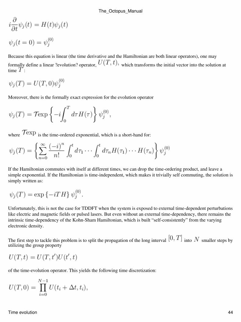
Because this equation is linear (the time derivative and the Hamiltonian are both linear operators), one may
formally define a linear ?evolution? operator, which transforms the initial vector into the solution attime :
Moreover, there is the formally exact expression for the evolution operator
where is the time-ordered exponential, which is a short-hand for:
If the Hamiltonian commutes with itself at different times, we can drop the time-ordering product, and leave asimple exponential. If the Hamiltonian is time-independent, which makes it trivially self commuting, the solution issimply written as:
Unfortunately, this is not the case for TDDFT when the system is exposed to external time-dependent perturbationslike electric and magnetic fields or pulsed lasers. But even without an external time-dependency, there remains theintrinsic time-dependency of the Kohn-Sham Hamiltonian, which is built “self-consistently” from the varyingelectronic density.
The first step to tackle this problem is to split the propagation of the long interval into smaller steps byutilizing the group property
of the time-evolution operator. This yields the following time discretization:
The_Octopus_Manual
Time evolution 44
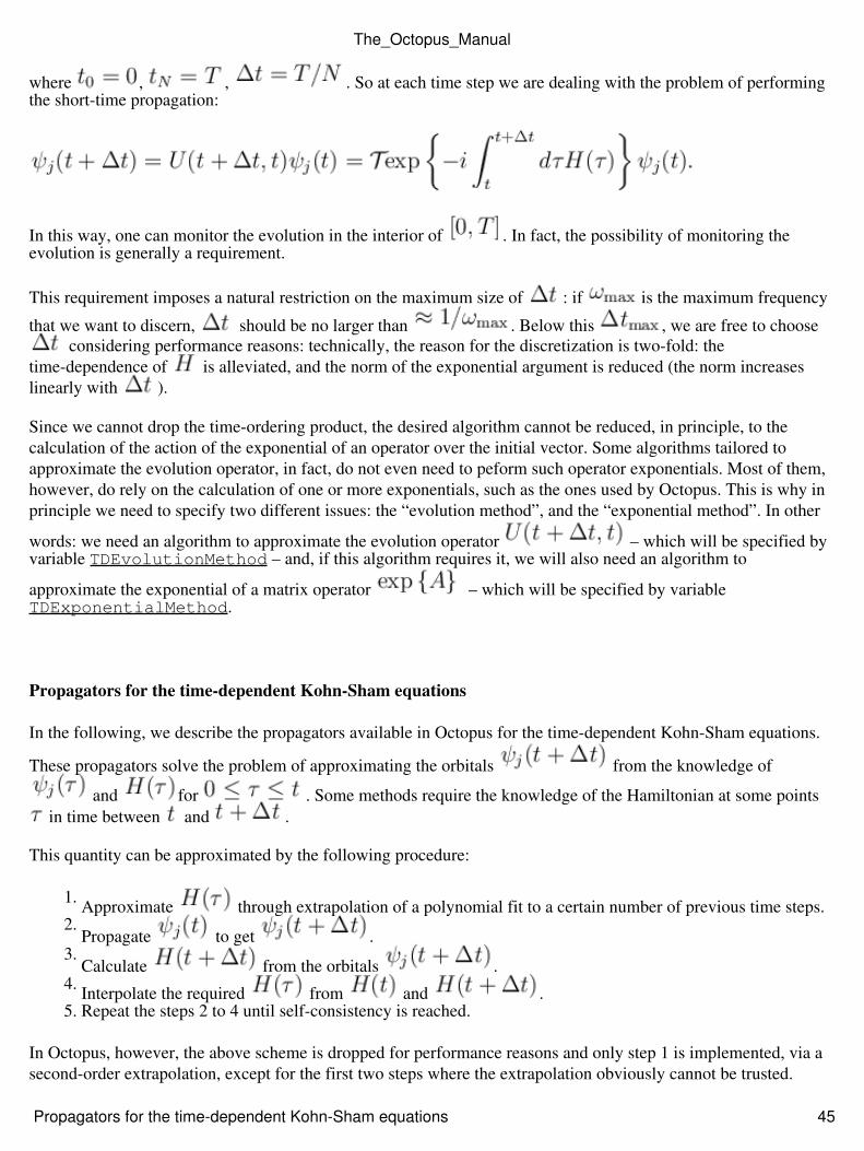
where , , . So at each time step we are dealing with the problem of performingthe short-time propagation:
In this way, one can monitor the evolution in the interior of . In fact, the possibility of monitoring theevolution is generally a requirement.
This requirement imposes a natural restriction on the maximum size of : if is the maximum frequency
that we want to discern, should be no larger than . Below this , we are free to choose considering performance reasons: technically, the reason for the discretization is two-fold: the
time-dependence of is alleviated, and the norm of the exponential argument is reduced (the norm increaseslinearly with ).
Since we cannot drop the time-ordering product, the desired algorithm cannot be reduced, in principle, to thecalculation of the action of the exponential of an operator over the initial vector. Some algorithms tailored toapproximate the evolution operator, in fact, do not even need to peform such operator exponentials. Most of them,however, do rely on the calculation of one or more exponentials, such as the ones used by Octopus. This is why inprinciple we need to specify two different issues: the “evolution method”, and the “exponential method”. In other
words: we need an algorithm to approximate the evolution operator – which will be specified byvariable TDEvolutionMethod – and, if this algorithm requires it, we will also need an algorithm to
approximate the exponential of a matrix operator – which will be specified by variableTDExponentialMethod.
Propagators for the time-dependent Kohn-Sham equations
In the following, we describe the propagators available in Octopus for the time-dependent Kohn-Sham equations.
These propagators solve the problem of approximating the orbitals from the knowledge of
and for . Some methods require the knowledge of the Hamiltonian at some points in time between and .
This quantity can be approximated by the following procedure:
Approximate through extrapolation of a polynomial fit to a certain number of previous time steps.1.
Propagate to get .2.
Calculate from the orbitals .3.
Interpolate the required from and .4.
Repeat the steps 2 to 4 until self-consistency is reached.5.
In Octopus, however, the above scheme is dropped for performance reasons and only step 1 is implemented, via asecond-order extrapolation, except for the first two steps where the extrapolation obviously cannot be trusted.
The_Octopus_Manual
Propagators for the time-dependent Kohn-Sham equations 45
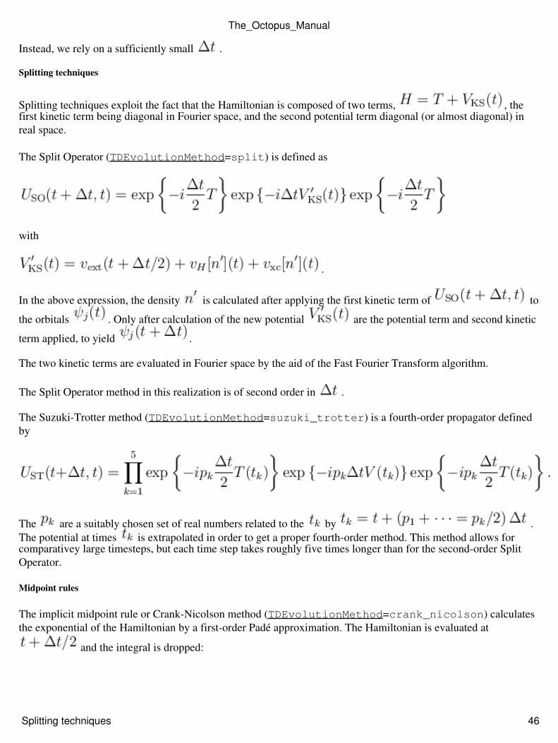
Instead, we rely on a sufficiently small .
Splitting techniques
Splitting techniques exploit the fact that the Hamiltonian is composed of two terms, , thefirst kinetic term being diagonal in Fourier space, and the second potential term diagonal (or almost diagonal) inreal space.
The Split Operator (TDEvolutionMethod=split) is defined as
with
.
In the above expression, the density is calculated after applying the first kinetic term of to
the orbitals . Only after calculation of the new potential are the potential term and second kinetic
term applied, to yield .
The two kinetic terms are evaluated in Fourier space by the aid of the Fast Fourier Transform algorithm.
The Split Operator method in this realization is of second order in .
The Suzuki-Trotter method (TDEvolutionMethod=suzuki_trotter) is a fourth-order propagator definedby
The are a suitably chosen set of real numbers related to the by .The potential at times is extrapolated in order to get a proper fourth-order method. This method allows forcomparativey large timesteps, but each time step takes roughly five times longer than for the second-order SplitOperator.
Midpoint rules
The implicit midpoint rule or Crank-Nicolson method (TDEvolutionMethod=crank_nicolson) calculatesthe exponential of the Hamiltonian by a first-order Padé approximation. The Hamiltonian is evaluated at
and the integral is dropped:
The_Octopus_Manual
Splitting techniques 46
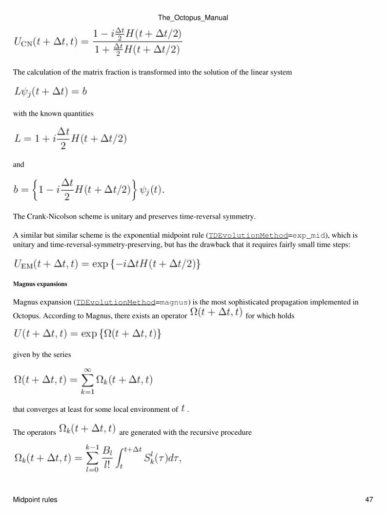
The calculation of the matrix fraction is transformed into the solution of the linear system
with the known quantities
and
The Crank-Nicolson scheme is unitary and preserves time-reversal symmetry.
A similar but similar scheme is the exponential midpoint rule (TDEvolutionMethod=exp_mid), which isunitary and time-reversal-symmetry-preserving, but has the drawback that it requires fairly small time steps:
Magnus expansions
Magnus expansion (TDEvolutionMethod=magnus) is the most sophisticated propagation implemented in
Octopus. According to Magnus, there exists an operator for which holds
given by the series
that converges at least for some local environment of .
The operators are generated with the recursive procedure
The_Octopus_Manual
Midpoint rules 47
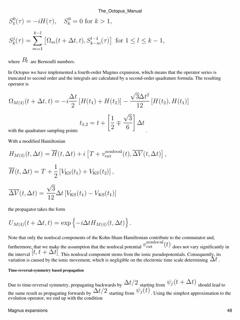
where are Bernoulli numbers.
In Octopus we have implemented a fourth-order Magnus expansion, which means that the operator series istruncated to second order and the integrals are calculated by a second-order quadrature formula. The resultingoperator is
with the quadrature sampling points .
With a modified Hamiltonian
the propagator takes the form
Note that only the nonlocal components of the Kohn-Sham Hamiltonian contribute to the commutator and,
furthermore, that we make the assumption that the nonlocal potential does not vary significantly in
the interval . This nonlocal component stems from the ionic pseudopotentials. Consequently, itsvariation is caused by the ionic movement, which is negligible on the electronic time scale determining .
Time-reversal-symmetry based propagation
Due to time-reversal symmetry, propagating backwards by starting from should lead to
the same result as propagating forwards by starting from . Using the simplest approximation to theevolution operator, we end up with the condition
The_Octopus_Manual
Magnus expansions 48
Rearranging the terms gives an approximation for the propagator:
This enforced time-reversal symmetry method is available in Octopus by setting(TDEvolutionMethod=etrs).
It is worthwhile to give a sidenote on the approximation of : for the etrs method the Hamiltonian
at time is not extrapolated, but rather built from the density , which, inturn, is calculated from the orbital estimate
There exists, however, also a variant TDEvolutionMethod=aetrs (approximated enforced time-reversal
symmetry) that performs a second-order polynomial extrapolation of , , to get
, which is about 40 % faster than etrs.
Approximations to the exponential of an operator
Most of the evolution methods described in the previous section require the calculation of the exponential of amatrix. Before going into the details of the TDExponentialMethod that Octopus provides, one generaldifficulty deserves mentioning.
In principle, we would like to calculate by first calculating and then applying thisresult to any vector . Unfortunately, the size of our Hamiltonian matrix is of the order which forbids itsfull storage in matrix form. Apart from that, methods to calculate the exponential of a matrix explicitly are limitedto a few thousand matrix elements. For this reason, we have to turn to iterative solutions that calculate
for a particular vector .
Polynomial expansions
The simplest possibility is to use the definition of the exponential of a matrix
to get the approximation of order (TDExponentialMethod=standard):
The_Octopus_Manual
Time-reversal-symmetry based propagation 49
amounts to the expansion of the exponential in the standard polynomial base
.
Experience shows that the choice gives particularly good results for our TDDFT implementation.
The standard polynomial basis is not the only possibility; Octopus also implements the expansion of theexponential in the Chebyshev basis:
with being the Chebyshev polynomial of order .
The truncation for both these expansions can be set by the input variable ExpOrder.
Krylov-subspace projection
The Krylov subspace of order for a given operator and vector is defined as
The idea is to find the element of that optimally approximates in a least-squaressense. It can be proven that this is given by
with being an orthonormal basis of calculated with the Lanczosprocedure. To get rid of the exponential, the approximation
is introduced. The object is also a result of the Lanczos procedure and of the small dimension which allows for direct calculation of the remaining exponential. So, we have
which can be selected by setting TDExponentialMethod=lanczos. When actually calculating the
exponential, Octopus recursively generates the quantities and until some convergence criterion –
The_Octopus_Manual
Polynomial expansions 50
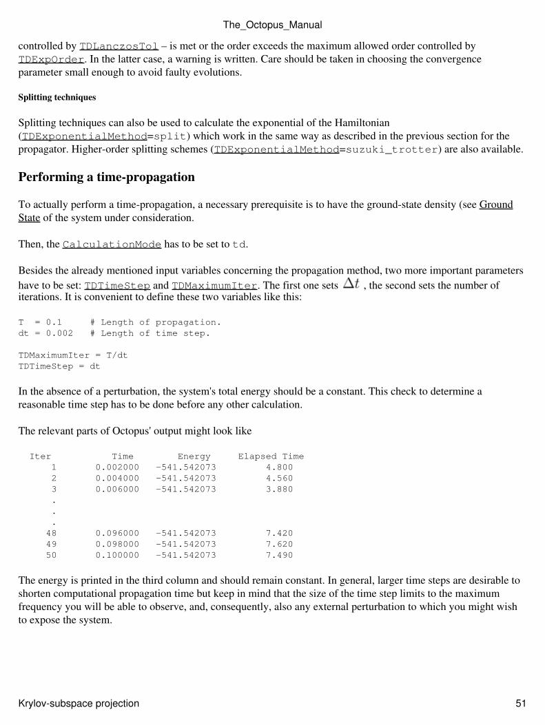
controlled by TDLanczosTol – is met or the order exceeds the maximum allowed order controlled byTDExpOrder. In the latter case, a warning is written. Care should be taken in choosing the convergenceparameter small enough to avoid faulty evolutions.
Splitting techniques
Splitting techniques can also be used to calculate the exponential of the Hamiltonian(TDExponentialMethod=split) which work in the same way as described in the previous section for thepropagator. Higher-order splitting schemes (TDExponentialMethod=suzuki_trotter) are also available.
Performing a time-propagation
To actually perform a time-propagation, a necessary prerequisite is to have the ground-state density (see GroundState of the system under consideration.
Then, the CalculationMode has to be set to td.
Besides the already mentioned input variables concerning the propagation method, two more important parametershave to be set: TDTimeStep and TDMaximumIter. The first one sets , the second sets the number ofiterations. It is convenient to define these two variables like this:
T = 0.1 # Length of propagation.dt = 0.002 # Length of time step.
TDMaximumIter = T/dtTDTimeStep = dt
In the absence of a perturbation, the system's total energy should be a constant. This check to determine areasonable time step has to be done before any other calculation.
The relevant parts of Octopus' output might look like
Iter Time Energy Elapsed Time 1 0.002000 -541.542073 4.800 2 0.004000 -541.542073 4.560 3 0.006000 -541.542073 3.880 . . . 48 0.096000 -541.542073 7.420 49 0.098000 -541.542073 7.620 50 0.100000 -541.542073 7.490
The energy is printed in the third column and should remain constant. In general, larger time steps are desirable toshorten computational propagation time but keep in mind that the size of the time step limits to the maximumfrequency you will be able to observe, and, consequently, also any external perturbation to which you might wishto expose the system.
The_Octopus_Manual
Krylov-subspace projection 51
External fields
Delta kick: Calculating an absorption spectrum
To obtain the linear optical absorption spectrum of the system, we follow the scheme proposed by Yabana andBertsch, and excite all frequencies of the system by giving some small momentum ( ) to the electrons. This isachieved by transforming the ground-state wavefunctions according to:
and then propagating these wavefunctions for some (finite) time. The spectrum can then be obtained from theexpression for the dipole strength function S(ω):
where the dynamical polarizability, α(ω), is essentially the Fourier transform of the dipole moment of the systemd(t):
With this definition, the Thomas-Reiche-Kuhn f-sum rule for the number of electrons, N, is given by the integral:
This sum rule can be used to check the quality of the calculations. Another check is energy conservation, whichTDDFT respects when no external field is applied.
To obtain a spectrum with such a recipe in Octopus one has to follow the steps:
Choose a system of linearly independent (can be non-orthogonal) axes (defined by the variableTDPolarization). The defaults are the 3 Cartesian axes.
1.
Add an electric kick using the variable TDDeltaStrength. Its value should be small so that we remainin the linear regime, but large enough to avoid numerical errors.
2.
Run a time-dependent simulation for the 3 independent directions. This involves running Octopus 3 times,changing the value of TDPolarizationDirection each time. After each run, move the filetd.general/multipoles to td.general/multipoles.X<tt>, where <tt>X is 1, 2, or 3.
3.
Run the utility oct-propagate_spectrum.4.
Lasers
To calculate non-linear optical properties, we follow the evolution of the system under the influence of a laser fieldthat is treated in the dipole approximation (although this constraint can be removed). The harmonic emissionspectrum can then be calculated from the acceleration of the dipole moment:
The_Octopus_Manual
External fields 52
During the propagation, charge density is absorbed at the boundaries of the simulation region, either by animaginary absorbing potential or a mask function. In the first case, we add to the Kohn-Sham potential a term
where Vabs is zero in the inner region of the simulation box, and rises smoothly till the edges. By adjusting both theheight and the shape of the potential, we can select which momenta are absorbed and prevent the unwantedreflections at the boundary. When using a mask, the wavefunction is multiplied in each time-step by a functionwhich is 1 in the inner simulation region and gradually goes to 0 at the borders:
The absorbed charge can be interpreted as an ionization probability and can be used to estimate the photo-electronspectra. The box size has to be big enough so that the physical system is not perturbed by the absorbingboundaries. Note that the wavefunctions are no longer normalized as the system slowly gets charged.
Symmetries
The dynamic polarizability (trivially related to optical absorption) is, in its most general form, a 3x3 tensor. Thereason is that we can shine light on the system polarized in any of the three Cartesian axes, and for each of thesethree cases measure how the dipole of the molecule oscillates along the three Cartesian axes. This usually meansthat to obtain the full dynamic polarizability of the molecule we usually need to apply 3 different perturbationsalong , by setting TDPolarizationDirection to 1, 2, or 3.
However, if the molecule has some symmetries, it is in general possible to reduce the total number of calculationsfrom 3 to 2, or even 1. This is explained in detail here. To use this formalism in Octopus, you can use the variablesTDPolarization, TDPolarizationDirection, TDPolarizationEquivAxis, andTDPolarizationWprime. The block TDPolarization defines a basis (not necessarily orthogonal) chosento maximize the number of equivalent axes, and TDPolarizationDirection, andTDPolarizationWprime are vectors specified in that basis. Let us give a couple of examples.
The methane molecule has Td symmetry, which means that the response is identical for all directions. This meansthat we only need one propagation to obtain the whole tensor. This propagation can be performed in any directionwe wish. So we could use the input
%TDPolarization 1 | 0 | 0 0 | 1 | 0 0 | 0 | 1%TDPolarizationDirection = 1TDPolarizationEquivAxis = 3%TDPolarizationWprime
The_Octopus_Manual
Lasers 53
0 | 0 | 1%
Note that we could have omitted the blocks TDPolarization and TDPolarizationWprime in the previousinput file, as these are their default values.
Now let us look at a linear molecule. In this case, you might think that we need two calculations to obtain thewhole tensor, one for the direction along the axis of the molecule, and another for the axis perpendicular to themolecule. The fact is that we need only one, in a specially chosen direction, so that our field has components bothalong the axis of the molecule and perpendicular to it. Let us assume that the axis of the molecule is oriented alongthe x-axis. Then we can use
%TDPolarization 1/sqrt(2) | -1/sqrt(2) | 0 1/sqrt(2) | 1/sqrt(2) | 0 1/sqrt(2) | 0 | 1/sqrt(2)%TDPolarizationDirection = 1TDPolarizationEquivAxis = 3%TDPolarizationWprime 0 | 0 | 1%
You should try to convince yourself that the three axes are indeed equivalent and linearly independent.
Finally, let us look at a general planar molecule (in the xy plane). In principle we need only two calculations(reduced to one if more symmetries are present, as for benzene). In this case we chose one of the polarization axeson the plane, and the other two rotated 45 degrees out of plane:
%TDPolarizationDirection 1/sqrt(2) | 0 | 1/sqrt(2) 1/sqrt(2) | 0 |-1/sqrt(2) 0 | 1 | 0%
TDPolarizationEquivAxis = 2
In this case, we need two runs, one for TDPolarizationDirection equal to 1, and another for it equal to 3.Note that if there are fewer than 3 equivalent axes, TDPolarizationWprime is irrelevant.
Previous Manual:Ground_State - Next Manual:Casida
Back to Manual <p class=newpage>
Casida Linear Response
Mark Casida's formulation of Linear-Response TDDFT allows calculations of the excitation energies of a finitesystem. For small molecules, this is normally the fastest way to calculate them.
The_Octopus_Manual
Symmetries 54
To perform a Casida calculation you first need a ground-state calculation and a calculation of unoccupied states;then you run the code with CalculationMode=casida.
This is an input file for a linear-response calculation of the nitrogen dimer, found atSHARE/testsuite/linear_response/01-casida.*.
%CalculationModegs | unocc | casida"ground_state_" | "unocc_states_" | "lrtddft_"1 | 2 | 3%
FromScratch = yes
bond_length = 2.0744
%Coordinates"N" | -bond_length/2 | 0.0 | 0.0 | no"N" | bond_length/2 | 0.0 | 0.0 | no%
%Species"N" | 14.0067000 | tm2 | 7 | 2 | 0%
BoxShape = sphere
Radius = 12.0Spacing = 0.36
SpinComponents = unpolarized
XFunctional = lda_xCFunctional = lda_c_vwn
MaximumIter = 200ConvRelDens = 1e-5
LCAOStart = lcao_fullLCAODimension = 18
EigenSolver = cg_newEigenSolverInitTolerance = 1e-2EigenSolverFinalTolerance = 1e-5EigenSolverFinalToleranceIteration = 6EigenSolverMaxIter = 20unocc_states_EigenSolverMaxIter = 1000
TypeOfMixing = broyden
NumberUnoccStates = 9
PoissonSolver = fft_corrected
The_Octopus_Manual
Casida Linear Response 55
Previous Manual:Time-Dependent - Next Manual:Linear_Response
Back to Manual <p class=newpage>
Sternheimer Linear Response
This part of the code is quite recent and it is being actively developed, so not all the features might be available inthe stable version.
Octopus can calculate dynamic polarizabilities and first-order hyperpolarizabilites in a linear-response schemeusing the Sternheimer equation. It also possible to calculate optical spectra with this technique, but it is slower thantime-evolution.
Ground state
The first thing we will need for linear response is a Ground State calculation. Unlike other techniques, when usingthe Sterheimer equation you needn't do a unoccupied-states calculation. To improve the convergence of thelinear-response calculation, it is better to use tightly converged wavefunctions. For example, you can add theseparameters to your gs calculation:
EigenSolverFinalTolerance = 1e-10ConvAbsDens = 1e-9
Input
The CalculationMode for polarizability calculations is em_resp. The main parameter you have to specify isthe frequency of the perturbation, given by the EMFreqs block. You can also add an imaginary part to thefrequency by setting the variable EMEta. Adding a small imaginary part is required if you want to get theimaginary part of the polarizability or to calculate polarizabilities near resonance; a reasonable value is 0.1 eV.
To get the hyperpolarizabilties, you also have to specify the variable EMHyperpol with the three coefficientswith respect to the base frequency; the three values must sum to zero.
Output
After running, for each frequency in the input file, Octopus will generate a subdirectory under em_resp/. In eachsubdirectory there is a file called alpha that contains the real part of the polarizability tensor αij and the averagepolarizability
The imaginary part η is written to file eta. If η > 0, there is also a file called cross_section_tensor thatcontains the photo-absorption cross section tensor for that frequency, related to the imaginary part of the
The_Octopus_Manual
Sternheimer Linear Response 56
polarizability ( ).
The hyperpolarizability will be in a file called beta at the base frequency, containing all the 27 components andsome reduced quantities:
Optionally, Born charges can also be calculated.
Finite differences
In this mode only static polarizability can be obtained. The calculation is done by taking the numerical derivativeof the energy with respect to an external static and uniform electric field. To use this, run withResponseMethod =finite_differences. Octopus will run several ground-state energy calculations andthen calculate the polarizability using a finite-differences formula for the derivative. The results will be in theem_resp_fd directory. Hyperpolarizability and Born charges can also be calculated.
Previous Manual:Casida - Next Manual:Spectrum_calculations
Back to Manual <p class=newpage>
Optimal Control
If you set CalculationMode = opt_control, you will be attempting to solve the Quantum Optimal ControlTheory (QOCT) equations. This tutorial introduces the basic theoretical concepts of QOCT, as well as theprocedure to perform basic QOCT calculations with octopus.
If you already know QOCT, you can skip the Theoretical Introduction.
Theoretical Introduction
The QOCT can be formulated in the following way:
We consider a quantum mechanical system, governed in a temporal interval [0,T] by the Hamiltonian .
The Hamiltonian depends parametrically on a "control parameter" . In the cases we are concerned with, thisis the temporal shape of an external electromagnetic field, typically the temporal shape of a laser pulse. This
Hamiltonian drives the system from one specified initial state to a final state , according toSchrödinger's equation:
The_Octopus_Manual
Output 57
We now wish to find the optimal control parameter such that it maximizes a given objective, which in generalshould be expressed as a functional, J1[Ψ] of the full evolution of the state. This search must be constrained for tworeasons: One, the control parameter must be constrained to physical values -- that is, the laser field cannot acquireunlimitedly large values. Two, the evolution of the state must obviously follow Schrödinger equation.
These considerations are translated into mathematical terms by prescribing the maximization of the followingfunctional:
J1[Ψ] is the objective functional. In this basic tutorial, we will be concerned with the case in which itdepends only on the value of the state at the end of the propagation, Ψ(T). Moreover, the functional is the
expectation value of some positive-definite operator :
•
should constrain the values of the control parameter. Typically, the idea is to maximize theobjective J1 while minimizing the fluence:
•
The constant α is usually called penalty.
The maximization of J3 must ensure the verification of Schrödinger's equation:•
The auxiliary state χ plays the role of a Lagrangian multiplier.
In order to obtain the threesome that maximizes this functional we must find the solution to thecorresponding Euler equation. The functional derivation leads to the QOCT equations:
The_Octopus_Manual
Theoretical Introduction 58
Population target: scheme of Zhu, Botina and Rabitz
An important case in QOCT is when we want to achieve a large transition probability from a specific initial state
into a final target state. That is, the operator is the projection onto one given target state, Ψt:
As observed by Zhu, Botina and Rabitz[1], for this case one can use an alternative definition of J3:
This alternative definition has the virtue of decoupling the equations for χ and Ψ:
These are the equation that we are concerned with in the present example.
The asymmetric double well: preparing the states
We are now going to solve the previous equations, for the case of attempting a transition from the ground state of agiven system, to the first excited state. The system that we have chosen is a one-dimensional asymmetric doublewell, characterized by the potential:
The_Octopus_Manual
Population target: scheme of Zhu, Botina and Rabitz 59
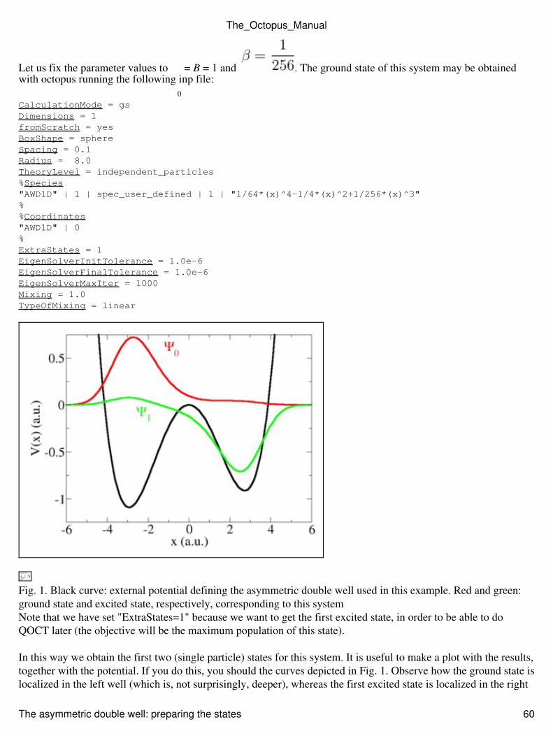
Let us fix the parameter values to ω
0
= B = 1 and . The ground state of this system may be obtainedwith octopus running the following inp file:
CalculationMode = gs Dimensions = 1 fromScratch = yesBoxShape = sphereSpacing = 0.1Radius = 8.0TheoryLevel = independent_particles%Species"AWD1D" | 1 | spec_user_defined | 1 | "1/64*(x)^4-1/4*(x)^2+1/256*(x)^3"%%Coordinates"AWD1D" | 0 %ExtraStates = 1EigenSolverInitTolerance = 1.0e-6EigenSolverFinalTolerance = 1.0e-6EigenSolverMaxIter = 1000Mixing = 1.0TypeOfMixing = linear
Fig. 1. Black curve: external potential defining the asymmetric double well used in this example. Red and green:ground state and excited state, respectively, corresponding to this systemNote that we have set "ExtraStates=1" because we want to get the first excited state, in order to be able to doQOCT later (the objective will be the maximum population of this state).
In this way we obtain the first two (single particle) states for this system. It is useful to make a plot with the results,together with the potential. If you do this, you should the curves depicted in Fig. 1. Observe how the ground state islocalized in the left well (which is, not surprisingly, deeper), whereas the first excited state is localized in the right
The_Octopus_Manual
The asymmetric double well: preparing the states 60
well. We are going to attempt to transfer the wavepacket from one side to the other. The energies of these twostates are -0.6206 a.u. and -0.4638, respectively.
Note that, in order to plot the functions, you will have to add to the inp file the variables Output andOutputHow.
Running octopus in QOCT mode
We now run the code with the following inp file:
Dimensions = 1fromScratch = yesCalculationMode = opt_control# ------------------# Grid# ------------------BoxShape = sphereSpacing = 0.1Radius = 8.0# ------------------# System# ------------------%Species"ADW1D" | 1 | spec_user_defined | 1 | "1/64*(x)^4-1/4*(x)^2+1/256*(x)^3"%%Coordinates"ADW1D" | 0%TheoryLevel = independent_particles# ------------------# TD RUN Parameters# ------------------stime = 100.0dt = 0.01TDPropagator = aetrsTDExponentialMethod = taylorTDExponentialOrder = 4TDLanczosTol = 5.0e-5TDMaximumIter = stime/dtTDTimeStep = dt# --------------# OCT parameters# --------------OCTPenalty =1.0OCTEps = 1.0e-6OCTMaxIter = 50OCTInitialState = oct_is_groundstateOCTTargetOperator = oct_tg_gstransformation%OCTTargetTransformStates0 | 1%OCTScheme = oct_algorithm_zbr98OCTDoubleCheck = yes#----------------------------# Laser field = Initial guess#-----------------------------
The_Octopus_Manual
Running octopus in QOCT mode 61
ampl = 0.06freq = 0.157 %TDExternalFieldselectric_field | 1 | 0 | 0 | freq | "envelope_function"%%TDFunctions"envelope_function" | tdf_cw | ampl%#----------------------------# Output#-----------------------------Output = wfsOutputHow = axis_xTDOutput = laser + td_occup
Let us go through some of the key elements of this inp file:
The first part of the file is just a repetition of the basic information already given in the inp file for theground state calculation: definition of the system through the Species block, specification of the mesh,etc.
•
Each QOCT run consists of a series of backward-forward propagations for both Ψ and χ; the variables inthe section "TD Run parameters" specify how those propagations are done. It is especially important to setthe total time of the propagation, which fixes the interval [0,T] mentioned above in the QOCT problemdefinition.
•
The next section ("OCT parameters") define the particular way in which OCT will be done:•
OCTScheme is the particular OCT algorithm to be used. For this example, we will use the one suggestedby Zhu, Botina and Rabitz[1]. This choice is "oct_algorithm_zbr98".
1.
OCTMaxIter sets a maximum number of iterations for the the ZBR98 algorithm. Each iterations involvesa forward and a backward propagation of the wavefunction.
2.
OCTEps sets a convergence threshold for the iterative scheme. This iterative scheme can be understood asa functional that processes an input control parameter and produces an output control parameters ,Upon convergence, input and output should converge and the iterations stopped. This will happenwhenever
is smaller than OCTEps. Note that this may never happen; there is no convergence guarantee.
3.
OCTPenalty sets the α penalty parameter described previously.4. OCTInitialState should specify the initial states from which the propagation starts. In most cases thiswill just be the ground state of the system -- this is the case for this example. The value"oct_is_groundstate" means that.
5.
OCTTargetOperator sets which kind of target operator ( , with the notation used above) will beused. As mentioned before, for this example we will be using a very common kind of target: the projection
onto a target state: . This is set by doing OCTTargetOperator =oct_tg_gstransformation. This means that the target state is constructed by taking a linear combination ofthe spin-orbitals that form the ground state. The particular linear combination to be used is set by the blockOCTTargetTransformStates.
6.
The_Octopus_Manual
Running octopus in QOCT mode 62
OCTTargetTransformStates. This is a block. Each line of the code refers to each of the spin orbitalsthat form the state the system; in this example we have a one-particle problem, and therefore one singlespin-orbital. This spin orbital will be a linear combination of the spin-orbitals calculated in the previousground-state run; each of the columns will contain the corresponding coefficient. In our case, we calculatedtwo spin-orbitals in the ground state run, therefore we only need two columns. And our target state issimply the first excited state, so the first column (coefficient of the ground state orbital) is zero, and thesecond column is one.
7.
OCTDoubleCheck simply asks the code to perform a final propagation with the best field it could findduring the QOCT iterative scheme, to check that it is really working as promised.
8.
The next section ("Laser field = Initial guess") simply specifies which is the initial laser field to be used as"initial guess". It is mandatory, since it not only provides with the initial guess for the "control parameter"
(which is simply a real function that specifies the temporal shape of the time-dependent externalperturbation), but also specifies what kind of external perturbation we are talking about: an electric fieldwith x, y or z polarization, a magnetic field, etc.
•
Finally, we would like to do cute plots with our results, so we add an "Output" section. This only applies ifwe have set OCTDoubleCheck=yes, since the code does not plot anything during the propagationsperformed in the QOCT iterations. The variables given will permit us to plot the shape of the wavefunctionduring the propagation, as well as the time-dependent electric field and the projection of the propagatingwave function onto the ground state and first excited state.
•
Even if this is a simple one-dimensional system, the run will take a few minutes because we are doing a lot ofpropagations. You will see how, at each iteration, some information is printed to standard output, e.g.:
****************** Optimal control iteration # 12 ****************** => J1 = 0.87422 => J = 0.54580 => J2 = -0.32842 => Fluence = 0.32842 => Penalty = 1.00000 => D[e,e'] = 1.66E-04**********************************************************************
The meaning of each number should be clear from the notation that we have introduced above. By construnction,the algorithm is "monotonously convergent", meaning that the value of J should increase. This does not guaranteethat the final value of J1 will actually approach one, which is our target (full overlap with the first excited state),but we certainly hope so.
At the end of the run it will do a "final propagation with the best field" (usually the one corresponding to the lastiteration). For this example, you will get something like:
*************** Final propagation with the best field **************** => J1 = 0.94924 => J = 0.61497 => J2 = -0.33427 => Fluence = 0.33427**********************************************************************
So we almost achieved a full transfer: .
The_Octopus_Manual
Running octopus in QOCT mode 63
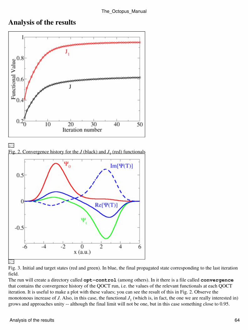
Analysis of the results
Fig. 2. Convergence history for the J (black) and J1 (red) functionals
Fig. 3. Initial and target states (red and green). In blue, the final propagated state corresponding to the last iterationfield.The run will create a directory called opt-control (among others). In it there is a file called convergencethat contains the convergence history of the QOCT run, i.e. the values of the relevant functionals at each QOCTiteration. It is useful to make a plot with these values; you can see the result of this in Fig. 2. Observe themonotonous increase of J. Also, in this case, the functional J1 (which is, in fact, the one we are really interested in)grows and approaches unity -- although the final limit will not be one, but in this case something close to 0.95.
The_Octopus_Manual
Analysis of the results 64
In the directory opt-control there are also some subdirectories called PsiT.0xx (xx running from 01 to 50,and laser.0xx. The former contain plots of the wavefunction at the end of the propagation, Ψ(T), at each of theQOCT iterative steps, while the latter contain the corresponding control parameter (it is called laser because it willalmost always represent a laser field).
The amount and type of information contained in each Psi.0xx directory will depend on the values that you setfor the variables Output and OutputHow. For our example, in the example that we have just run, it will containthe wavefunctions of the states (only one in our case) along the x axis (since it is just a one dimensional system).
If you perform many iterations, the amount of disk space needed to save all those files may be large, and you maywant to disable the writing of all the information corresponding to the intermediate iterations. This can be turnedon and off through the variable OCTDumpIntermediate.
There is also a directory called initial, useful to plot the initial state; a directory called target, that containsthe target state; and a directory called final that contains the state at the end of the propagation corresponding tothe last QOCT iteration. Fig. 3 is a plot constructed with the information contained in these directories. Note thatwhile the initial and target states have no imaginary part, the final propagated wavefunction is complex, andtherefore we have to plot both the real and the imaginary part.
In the directories laser.0xx you will find a file called cp which contains the control parameter for thecorresponding QOCT iteration. Another file, called fluence informs about the corresponding fluence. Theformat of file cp is simple: first column is time, second and third column are the real and imaginary part of thecontrol parameter. Since is defined to be real in our formulation, the last column should be null. Finally, thedirectory laser.bestJ1 will obviously contain the control parameter corresponding to the iteration thatproduced the best J1.
References
? 1.0 1.1 W. Zhu, J. Botina and H. Rabitz, J. Chem. Phys. 108, 1953 (1998)1.
Previous Tutorial:Geometry optimization - Next Tutorial:Open boundaries
Back to Tutorial <p class=newpage>
Geometry Optimization
To perform a geometry optimization with octopus one should set the CalculationMode to go. octopus uses theminimization routines from GSL. The method to be used should be set using the variable GOMethod.
The stopping criteria can be set with the variables GOTolerance and GOMinimumMove . Then minimizationwill be stopped when all forces on ions are smaller than GOTolerance or when all species coordinates changeless than GOMinimumMove during on minimization step. If none of the previous criteria is matched after anumber of minimization steps equal to GOMaxIter then the minimization will be stopped with an error message.
After each minimization step taken by the GSL algorithms octopus will write the current geometry to a file namedgo.XXXX.xyz (XXXX is the iteration number) in the directory geom. As an extra information, the title of thexyz file (second line) contains the total energy.
The_Octopus_Manual
References 65
Note that octopus is not particularly efficient in performing geometry optimizations and many times, if thestopping criteria are too small, the GSL routines will return an error message stating that they were unable toimprove the solution.
At the end of the run, if the minimization was successful, the minimized geometry will be written to a file namedmin.xyz in the working directory. <p class=newpage>
Advanced ways of running Octopus
Parallel Octopus
Octopus can be run in multi-tentacle (parallel) mode if you have configured it that way when you compiled andinstalled it. There are four possible parallelization strategies: domains, states, spin/k-points, and electron-hole pairs(only for Casida). You do not need to specify in the input file what kind of ParallelizationStrategy youwant to use as Octopus can find reasonable defaults. However, the experienced user may want to tune this variable.
Parallel in States
The first strategy is parallel in states. This means that each processor takes some states and propagates themindependently of the others.
To use this include
ParallelizationStrategy = par_states
in your input file.
This is clearly the most efficient (and simplest) way of parallelizing the code if the number of states is much largerthan the number of processors available (which is usually the case for us). You can expect a more or less linearspeed-up with number of processors until you reach around 5 states/processor. Beyond this it starts to saturate.
Parallel in Domains
When running parallel in "domains", octopus divides the simulation region (the box) into separate regions(domains) and assigns each of of these to a different processor. This allows it not only to speed up the calculation,but also to divide the memory among the different processors. The first step of this process, the splitting of the box,is in general a very complicated process. Note that we are talking about a simulation box of an almost arbitraryshape, and of an arbitrary number of processors. Furthermore, as the communication between processors growsproportionally to the surface of the domains, one should use an algorithm that divides the box such that eachdomain has the same number of points, and at the same time minimizes the total area of the domains. Octopus usesthe METIS library to make this domain decomposition of the space, METIS is included in the source code ofOctopus and will be used by default.
So for example, if you are planning to run the ground state of Na there's only one choice:
ParallelizationStrategy = par_domains
The_Octopus_Manual
Advanced ways of running Octopus 66
Octopus will then partition the real-space mesh and compute the resulting pieces on different nodes. Later whenyou plan to do time propagations you have more choices at hand. You could run only parallel in states
ParallelizationStrategy = par_states
or in domains (as above), or you can decide to employ both parallelization strategies
ParallelizationStrategy = par_domains + par_states
Problems with parallelization
The parallelization is only effective if a sufficiently large amount of load is given to each node. Otherwisecommunication dominates. In that case one should do the calculation in serial. This happens, for example, if youattempt to do parallelization in real-space domains, but your grid does not have too many points. If the code detectsthat the number of points per node is not large enough, it gives the warning:
** Warning:** From node = 0** I have less elements in a parallel group than recommended.** Maybe you should reduce the number of nodes
Compiling and running in parallel
The steps to compile and use octopus in parallel are:
1) use the --enable-mpi in the configuration script
2) give to octopus the libraries, etc. necessary to compile a parallel code. When you install mpich in your system, itcreates a series of programs called mpicc, mpif77, mpif90, etc. These are wrappers that call the specific compilerwith the appropriate flags, libraries, etc. This means that to compile octopus in parallel you'll need mpif90. Pleasecheck that this is present in your system (perhaps in /usr/local/bin if you compiled mpich from the sources).Octopus will try to find this compiler, but it may not be able to find it for several reasons:
mpif90 is _not_ in the path.•
there is another f90 compiler specified by the user/system. This means that if you have the variable FCdefined when you run the configure script, octopus will use the fortran compiler specified by that variable,and will not try to find mpif90. Then, the configuration fails.
•
export FC=<whatever path>/mpif90export FCFLAGS=<whatever flags>./configure --enable-mpi
It is wise to also set the FCFLAGS, as octopus cannot tell which fortran compiler you are using if you compile withmpif90.
3) Now you just have to run octopus in parallel (this step depends on your actual system, you may have to usempirun or mpiexec to accomplish it).
The_Octopus_Manual
Parallel in Domains 67
In some run modes (e.g., td), you can use the multi-level parallelization, i.e., to run in parallel in more than oneway at the same time. In the td case, you can run parallel in states and in domains at the same time. In order tofine-tune this behavior, please take a look at the variables ParallelizationStrategy andParallelizationGroupRanks. In order to check if everything is OK, take a look at the output of octopus inthe "Parallelization" section. This is an example:
************************** Parallelization ***************************Octopus will run in *parallel*Info: Number of nodes in par_states group: 8 ( 62)Info: Octopus will waste at least 9.68% of computer time**********************************************************************
In this case, Octopus runs in parallel only in states, using 8 processors (for 62 states). Furthermore, some of theprocessors will be idle for 9.68% of the time (this is not that great, so maybe a different number of processorswould be better in this case).
Multi-Dataset Mode
You can perform multiple runs with a single input file by using CalculationMode as a block. This is typicallydone for convenience to combine runs in different modes whose input files differ by only a few lines.
The first line is a list of calculation modes, the second is labels (optional; default is dsXX_ where XX=01, 02, ...),and the third is the order for the runs (optional; default is the order listed). The labels will be used as prefixes forthe output directories such as restart, static, td... etc., and can also be used as prefixes to variables toindicate that they apply only to that dataset's calculation.
An example from testsuite/finite_system_1d/01-hydrogen.01-ground_state.inp:
%CalculationMode gs | unocc "ground_state_" | "excited_states_" 1 | 2%excited_states_RestartDir = "ground_state_restart"excited_states_ExtraStates = 9
Passing arguments from environment variables
Octopus can also read input variables from the environment variables of the shell. This is especially useful if youwant to call octopus from scripts or if you want to pass one-time arguments when running Octopus.
To activate this feature you must first set OCT_PARSE_ENV to some value, for example in sh/bash
$ export OCT_PARSE_ENV=1
After that, to pass an input variable to octopus, you must prepend the name of the variable by 'OCT_', forexample:
$ export OCT_Radius=10
The_Octopus_Manual
Compiling and running in parallel 68
After that you can run Octopus as usual.
You can also pass the variables in the same command line:
$ OCT_PARSE_ENV=1 OCT_Radius=10 octopus
If you set a variable both from the input file and as a environment variable, the environment variable takesprecedence. Be careful with this behaviour. Blocks are not supported (suggestions as how to elegantly put a blockinside of environment variables are welcome).
There is an additional environment variable OCTOPUS_SHARE that can be set to specify the location of thevariables file used by the parser. If this environment variable is not set, the default is as set by the configurescript, namely prefix/share/octopus. You can set this to something else if necessary, for example tohandle moving an executable from one machine to another, where the original path does not exist on the newmachine.
Examples
For example this is a simple script that helps to determine the optimal Radius of the simulation box (an inp filewith the rest of the parameters has to be provided):
export OCT_PARSE_ENV=1for OCT_Radius in `seq 5 16`do export OCT_Radius octopus >& out-$OCT_Radius energy=`grep Total static/info | head -1 | cut -d "=" -f 2` echo $OCT_Radius $energydone
Previous Manual:Geometry_Optimization - Next Manual:External utilities:oct-atomic occupations
Back to Manual <p class=newpage>
Utilities<p class=newpage>
oct-atomic_occupations
This script prints out to standard output the electronic configuration of a given atom, and the way in which thiselectronic configuration should be reflected in the Occupations block of a corresponding Octopus input file.
Options
-s species
species should be the atomic symbol (e.g. Na, Au, etc).
The_Octopus_Manual
Utilities 69
-h
Show a brief summary of command line options.
Examples
$ oct-atomic_occupations -s Na
$ oct-atomic_occupations -s Ti_sc
$ for x in \$(cat /usr/share/octopus/PP/defaults | awk '{print \$1}')> do oct-atomic_occupations -s $x> done
Previous Manual:Advanced ways of running Octopus - Next Manual:External utilities:oct-casida_spectrum
Back to Manual <p class=newpage>
oct-casida_spectrum
NAME
oct-casida_spectrum - Broadens the linear-response spectra from the Casida run mode.
SYNOPSIS
oct-casida_spectrum
[oct-casida_spectrum does not read standard input: all standard input will be simply ignored. An input file namedinp must be present in the running directory. Also, oct-casida_spectrum accepts no command line arguments,since there is not a standard way to do this with Fortran 90.]
DESCRIPTION
This program is one of the Octopus utilities.
It post-processes the files casida/casida, casida/petersilka and casida/eps_diff, that containthe excitation energies and oscillator strengths.
The parameters of the spectrum can be set using the variables CasidaSpectrumBroadening,CasidaSpectrumMinEnergy, CasidaSpectrumMaxEnergy, and CasidaSpectrumEnergyStep.
The man pages of Octopus and of the auxiliary Octopus sub-programs (oct-something) are not intended to containthe documentation of the programs, but only their basic description. For where to find more documentation, see theSEE ALSO section below.
The_Octopus_Manual
Options 70
AUTHOR
Written by M. A. L. Marques, A. Castro, A. Rubio, C. A. Rozzi, F. Lorenzen, H. Appel and X. Andrade.
REPORTING BUGS
Report bugs through the <[email protected]> mailing list.
COPYRIGHT
Copyright (C) 2006 M. A. L. Marques, A. Castro, A. Rubio, C. A. Rozzi, F. Lorenzen, H. Appel and X. Andrade.
This is free software; see the source for copying conditions. There is NO warranty; not even forMERCHANTABILITY or FITNESS FOR A PARTICULAR PURPOSE.
SEE ALSO
The largest source of documentation is expected to be at the Octopus wiki:http://www.tddft.org/programs/octopus/wiki/.
At the usual standard locations, you will also find an info file octopus.info.
Previous Manual:External utilities:oct-atomic_occupations - Next Manual:External utilities:oct-center-geom
Back to Manual <p class=newpage>
oct-center-geom
NAME
oct-center-geom - Centers a molecule's geometry
SYNOPSIS
oct-center-geom
[oct-center-geom does not read the standard input: all standard input will be simply ignored. An input file namedinp must be present in the running directory. Also, oct-center-geom accepts no command-line arguments, sincethere is not a standard way to do this with Fortran 90.]
DESCRIPTION
This program is one of the Octopus utilities.
It reads the coordinates defined in the inp file, and constructs an output xyz file, that will be calledadjusted.xyz file, that describes the same system but in which the atomic coordinates are centered, and(optionally) has the axes aligned.
The_Octopus_Manual
AUTHOR 71
To control the orientation of the centered molecule there are two parameters: MainAxis and AxisType.
Do not forget then to change your input file to use this file instead of your old geometry (by changingXYZCoordinates='adjusted.xyz').
Be careful with units, this utility honours the Units, UnitsInput and UnitsOutput variables, so theadjusted.xyz file will be in the specified output units.
The man pages of Octopus and of the auxiliary Octopus sub-programs (oct-something) are not intended to containthe documentation of the programs, but only their basic description. For where to find more documentation, see theSEE ALSO section below.
AUTHOR
Written by M. A. L. Marques, A. Castro, A. Rubio, C. A. Rozzi, F. Lorenzen, H. Appel and X. Andrade.
REPORTING BUGS
Report bugs through the <[email protected]> mailing list.
COPYRIGHT
Copyright (C) 2006 M. A. L. Marques, A. Castro, A. Rubio, C. A. Rozzi, F. Lorenzen, H. Appel and X. Andrade.
This is free software; see the source for copying conditions. There is NO warranty; not even forMERCHANTABILITY or FITNESS FOR A PARTICULAR PURPOSE.
SEE ALSO
The largest source of documentation is expected to be at the Octopus wiki:http://www.tddft.org/programs/octopus/wiki/.
At the usual standard locations, you will also find an info file, octopus.info.
Previous Manual:External utilities:oct-casida_spectrum - Next Manual:oct-propagate_spectrum
Back to Manual <p class=newpage>
oct-propagate_spectrum
NAME
oct-propagate_spectrum - Calculates the absorption cross section tensor from the results of a time-propagation run.
The_Octopus_Manual
DESCRIPTION 72
SYNOPSIS
oct-propagate_spectrum
[oct-propagate_spectrum does not read the standard input: all standard input will be simply ignored. An input filenamed inp must be present in the running directory. Also, oct-propagate_spectrum accepts no command linearguments, since there is not a standard way to do this with Fortran 90.]
DESCRIPTION
This program is one of the Octopus utilities.
The man pages of Octopus and of the auxiliary Octopus sub-programs (oct-something) are not intended to containthe documentation of the programs, but only their basic description. For where to find more documentation, see theSEE ALSO section below.
This utility generates the dipole strength function of the given system. Its main input is the td.general/multipolesfile. Output is written to a file called spectrum. This file is made of two columns: energy (in eV or a.u., dependingon the units specified in the input file), and dipole strength function (in 1/eV, or 1/a.u., idem).
In the input file, the user may set the PropagationSpectrumTransform (this should be set to ?sine? forproper use), the PropagationSpectrumDampMode (recommended value is ?polynomial?, which ensuresfulfilling of the N-sum rule), the PropagationSpectrumStartTime, thePropagationSpectrumEndTime, the PropagationSpectrumEnergyStep, and thePropagationSpectrumMaxEnergy.
AUTHOR
Written by M. A. L. Marques, A. Castro, A. Rubio, C. A. Rozzi, F. Lorenzen, H. Appel and X. Andrade.
REPORTING BUGS
Report bugs through the <[email protected]> mailing list.
COPYRIGHT
Copyright (C) 2006 M. A. L. Marques, A. Castro, A. Rubio, C. A. Rozzi, F. Lorenzen, H. Appel and X. Andrade.
This is free software; see the source for copying conditions. There is NO warranty; not even forMERCHANTABILITY or FITNESS FOR A PARTICULAR PURPOSE.
SEE ALSO
The largest source of documentation is expected to be at the Octopus wiki:http://www.tddft.org/programs/octopus/wiki/.
At the usual standard locations, you will also find an info file, octopus.info.
The_Octopus_Manual
SYNOPSIS 73
Previous Manual:External utilities:oct-center-geom - Next Manual:External utilities:oct-display_partitions
Back to Manual <p class=newpage>
oct-display_partitions
NAME
oct-display_partitions - Graphical representation of the mesh partitions.
SYNOPSIS
oct-display_partitions
[oct-display_partitions does not read the standard input: all standard input will be simply ignored. Also,oct-display_partitions accepts no command line arguments.]
DESCRIPTION
This program is one of the octopus utilities.
It is a script to use gnuplot to plot the partitioning of the mesh. The files TO DO mesh_partition.??? asproduced in debug/mesh_partition by the Octopus debug mode have to be present in the current workingdirectory when this script is invoked. The plot can be found in the file mesh_partitions.png. This scriptgenerates a gnuplot-script called mesh_partitions_index.gp which is stored in the current workingdirectory and can be loaded into gnuplot manually. With:
$ gnuplot> load mesh_partitions_index.gp$ gnuplot> set term x11$ gnuplot> replot
the plot can be reproduced and shown on the screen so that rotating and zooming is possible.
The man pages of Octopus and of the auxiliary Octopus sub-programs (oct-something) are not intended to containthe documentation of the programs, but only their basic description. For where to find more documentation, see theSEE ALSO section below.
AUTHOR
Written by H. Appel.
REPORTING BUGS
Report bugs through the <[email protected]> mailing list.
The_Octopus_Manual
SEE ALSO 74
COPYRIGHT
Copyright (C) 2005 H. Appel.
This is free software; see the source for copying conditions. There is NO warranty; not even forMERCHANTABILITY or FITNESS FOR A PARTICULAR PURPOSE.
SEE ALSO
The largest source of documentation is expected to be at the Octopus wiki:http://www.tddft.org/programs/octopus/wiki/.
At the usual standard locations, you will also find an info file, octopus.info.
Previous Manual:oct-propagate_spectrum - Next Manual:External utilities:oct-harmonic-spectrum
Back to Manual <p class=newpage>
oct-harmonic-spectrum
NAME
oct-harmonic-spectrum - Calculates the harmonic spectrum.
SYNOPSIS
oct-harmonic-spectrum
[oct-harmonic-spectrum does not read the standard input: all standard input will be simply ignored. An input filenamed inp must be present in the running directory. Also, oct-harmonic-spectrum accepts no command linearguments, since there is not a standard way to do this with Fortran 90.]
DESCRIPTION
This program is one of the Octopus utilities.
TO DO MISSING SHORT DESCRIPTION OF THE PROGRAM
The man pages of Octopus and of the auxiliary Octopus sub-programs (oct-something) are not intended to containthe documentation of the programs, but only their basic description. For where to find more documentation, see theSEE ALSO section below.
AUTHOR
Written by M. A. L. Marques, A. Castro, A. Rubio, C. A. Rozzi, F. Lorenzen, H. Appel and X. Andrade.
The_Octopus_Manual
COPYRIGHT 75
REPORTING BUGS
Report bugs through the <[email protected]> mailing list.
COPYRIGHT
Copyright (C) 2006 M. A. L. Marques, A. Castro, A. Rubio, C. A. Rozzi, F. Lorenzen, H. Appel and X. Andrade.
This is free software; see the source for copying conditions. There is NO warranty; not even forMERCHANTABILITY or FITNESS FOR A PARTICULAR PURPOSE.
SEE ALSO
The largest source of documentation is expected to be at the Octopus wiki:http://www.tddft.org/programs/octopus/wiki/.
At the usual standard locations, you will also find an info file, octopus.info.
Previous Manual:External utilities:oct-display_partitions - Next Manual:External utilities:oct-vibrational_spectrum
Back to Manual <p class=newpage>
oct-vibrational_spectrum
REDIRECT Manual:oct-vibrational spectrum1.
<p class=newpage>
oct-rotatory_strength
NAME
oct-rotatory_strength - Calculates the circular dichroism spectrum from a time-propagation run.
SYNOPSIS
oct-rotatory_strength
[oct-rotatory_strength does not read the standard input: all standard input will be simply ignored. An input filenamed inp must be present in the running directory. Also, oct-rsf accepts no command line arguments, since thereis not a standard way to do this with Fortran 90.]
DESCRIPTION
This program is one of the octopus utilities.
The_Octopus_Manual
REPORTING BUGS 76
TO DO MISSING SHORT DESCRIPTION OF THE PROGRAM
The man pages of Octopus and of the auxiliary Octopus sub-programs (oct-something) are not intended to containthe documentation of the programs, but only their basic description. For where to find more documentation, see theSEE ALSO section below.
AUTHOR
Written by M. A. L. Marques, A. Castro, A. Rubio, C. A. Rozzi, F. Lorenzen, H. Appel and X. Andrade.
REPORTING BUGS
Report bugs through the <[email protected]> mailing list.
COPYRIGHT
Copyright (C) 2006 M. A. L. Marques, A. Castro, A. Rubio, C. A. Rozzi, F. Lorenzen, H. Appel and X. Andrade.
This is free software; see the source for copying conditions. There is NO warranty; not even forMERCHANTABILITY or FITNESS FOR A PARTICULAR PURPOSE.
SEE ALSO
The largest source of documentation is expected to be at the Octopus wiki:http://www.tddft.org/programs/octopus/wiki/.
At the usual standard locations, you will also find an info file, octopus.info.
Previous Manual:oct-vibrational_spectrum - Next Manual:External utilities:oct-run_periodic_table
Back to Manual <p class=newpage>
oct-run_periodic_table
NAME
oct-run_periodic_table - run octopus for atoms
SYNOPSIS
oct-run_periodic_table [ option ] ...
DESCRIPTION
This script is one of the octopus utilities.
Simple script to run octopus for all atoms in the periodic table for which pseudopoentials are available.
The_Octopus_Manual
DESCRIPTION 77
-h
Show this message
-n
Run in dry run mode (show what would be executed)
-s species
Run octopus for given species.
-a
Run octopus for all atoms
-r
Do a restart, i.e. do not use fromScratch=yes.
-t temperature
Run with electronic temperature.
-e no_states
Use extra states
-x octopus_executable
-d defaults_file_for_pseudopotentials
The man pages of Octopus and of the auxiliary Octopus sub-programs (oct-something) are not intended to containthe documentation of the programs, but only their basic description. For where to find more documentation, see theSEE ALSO section below.
EXAMPLES
The following command would run the octopus executable to calculate the He atom.
$ oct-run_periodic_table -s He -x octopus
AUTHOR
Written by H. Appel.
The_Octopus_Manual
DESCRIPTION 78
REPORTING BUGS
Report bugs to <[email protected]>.
COPYRIGHT
Copyright (C) 2005 H. Appel.
This is free software; see the source for copying conditions. There is NO warranty; not even forMERCHANTABILITY or FITNESS FOR A PARTICULAR PURPOSE.
SEE ALSO
The largest source of documentation is expected to be at the Octopus wiki:http://www.tddft.org/programs/octopus/wiki/.
At the usual standard locations, you will also find an info file, octopus.info.
Previous Manual:External utilities:oct-rotatory_strength - Next Manual:External utilities:oct-run_regression_test.pl
Back to Manual <p class=newpage>
oct-run_regression_test.pl
NAME
oct-run_regression_test.pl - Script to create and run octopus regression tests
SYNOPSIS
oct-run_regression_test.pl [ option ] ... [ file ] ...
DESCRIPTION
This script is one of the octopus utilities.
This script can be used to generate and run the octopus regression tests.
The man pages of octopus and of the auxiliary octopus sub-programs (oct-something) are not intended to containthe documentation of the programs, but only their basic description. For where to find more documentation, see the"SEE ALSO" section below.
-n
Dry run. Don't run the test. Only print what would be executed.
-v
The_Octopus_Manual
REPORTING BUGS 79
Run in verbose mode. Useful for debugging the script.
-h
Show a brief summary of command line options.
-e *file*
Specify the name of the Octopus executable. The default is octopus.
-c *file*
Create a template for a Octopus regression test. This should always be used if you create a new regressiontest.
-f *file*
This option specifies the input file for a regression test.
-d *directory*
Use *directory* as working directory. The default is a randomly generated directory in /tmp.
-i
Print content of the octopus inputfile which is used for the current test to stdout.
-p
Preserve working directory. Don't clean up the temporary working directory after the run.
EXAMPLES
To create a template for a regression test run e.g.
$ oct-run_regression_test.pl -c finite_systems_3d/sodium.test
Running a test can be achieved with
$ oct-run_regression_test.pl -f finite_systems_3d/sodium.test
If a test run fails it might be useful for bug tracing to preserve the working directory of this run and to print out theinput file
$ oct-run_regression_test.pl -pi -f finite_systems_3d/sodium.test
Run a MPI test with a local directory as working directory
$ oct-run_regression_test.pl -d./tmp -f benzene.test -e `pwd`/../src/octopus-mpi
The_Octopus_Manual
DESCRIPTION 80
AUTHOR
Written by H. Appel.
REPORTING BUGS
Report bugs to <[email protected]>.
COPYRIGHT
Copyright (C) 2005 H. Appel.
This is free software; see the source for copying conditions. There is NO warranty; not even forMERCHANTABILITY or FITNESS FOR A PARTICULAR PURPOSE.
SEE ALSO
The largest source of documentation is expected to be at the Octopus wiki:http://www.tddft.org/programs/octopus/wiki/.
Previous Manual:External utilities:oct-run_periodic_table - Next Manual:External utilities:oct-run_testsuite
Back to Manual <p class=newpage>
oct-run_testsuite
NAME
oct-run_testsuite - Script to run the octopus testsuite.
SYNOPSIS
oct-run_testsuite [ option ] ...
DESCRIPTION
This script is one of the octopus utilities.
This script runs the octopus testsuite.
The man pages of Octopus and of the auxiliary Octopus sub-programs (oct-something) are not intended to containthe documentation of the programs, but only their basic description. For where to find more documentation, see theSEE ALSO section below.
-h
Prints out a short help message.
The_Octopus_Manual
AUTHOR 81
-n
Run in dry mode (show what would be executed).
-f
Run full testsuite.
-l
Local run.
-p prefix
Installation prefix [default: /usr]
-m address Mail report to address
EXAMPLES
TO DO MISSING EXAMPLES
AUTHOR
Written by H. Appel.
REPORTING BUGS
Report bugs to <[email protected]>.
COPYRIGHT
Copyright (C) 2005 H. Appel.
This is free software; see the source for copying conditions. There is NO warranty; not even forMERCHANTABILITY or FITNESS FOR A PARTICULAR PURPOSE.
SEE ALSO
The largest source of documentation is expected to be at the Octopus wiki:http://www.tddft.org/programs/octopus/wiki/.
Previous Manual:External utilities:oct-run_regression_test.pl - Next Manual:External utilities:oct-xyz-anim
Back to Manual <p class=newpage>
The_Octopus_Manual
DESCRIPTION 82
oct-xyz-anim
NAME
oct-xyz-anim - Constructs an "animated" xyz file from a time-propagation file where the atoms were allowed tomove
SYNOPSIS
oct-xyz-anim
[oct-xyz-anim does not read the standard input: all standard input will be simply ignored. An input file named inpmust be present in the running directory. Also, oct-xyz-anim accepts no command line arguments, since there isnot a standard way to do this with Fortran 90.]
DESCRIPTION
This program is one of the Octopus utilities. It reads out the td.general/coordinates file, and makes amovie in XYZ format, called 'movie.xyz'.
The man pages of Octopus and of the auxiliary Octopus sub-programs (oct-something) are not intended to containthe documentation of the programs, but only their basic description. For where to find more documentation, see theSEE ALSO section below.
AUTHOR
Written by M. A. L. Marques, A. Castro, A. Rubio, C. A. Rozzi, F. Lorenzen, H. Appel and X. Andrade.
REPORTING BUGS
Report bugs through the <[email protected]> mailing list.
COPYRIGHT
Copyright (C) 2006 M. A. L. Marques, A. Castro, A. Rubio, C. A. Rozzi, F. Lorenzen, H. Appel and X. Andrade.
This is free software; see the source for copying conditions. There is NO warranty; not even forMERCHANTABILITY or FITNESS FOR A PARTICULAR PURPOSE.
SEE ALSO
The largest source of documentation is expected to be at the Octopus wiki:http://www.tddft.org/programs/octopus/wiki/.
At the usual standard locations, you will also find an info file, octopus.info.
Previous Manual:External utilities:oct-run_testsuite - Next Manual:External utilities:Visualization
The_Octopus_Manual
oct-xyz-anim 83
Back to Manual <p class=newpage>
Visualization
Every given number of time iterations, or after ground-state calculations, some of the functions that characterisethe system may be written to disk so that they may be analized. Files are written within static/ output directoryafter the self-consistent field, or within td.x/ directories, during evolution, where ?x? stands for the iterationnumber at which each write is done.
The function that you want to plot is selected by the Output variable and the output format is chosen by theOutputHow.
dx
This is an OpenDX network, aimed at the visualization of wavefunctions. To be able to use it, you need to haveproperly installed the OpenDX program, as well as the Chemistry extensions developed at the Cornell TheoryCenter (http://www.tc.cornell.edu/Services/Visualization/). Please take a look here to see how to obtain and installthis software.
Once these are working, you may follow the tutorial for the benzene molecule.
XCrySDen
Atomic coordinates (finite or periodic), forces, and functions on a grid can be plotted with the free programXCrySDen. Its XSF format also can be read by V_Sim and Vesta. Beware, these all probably assume that youroutput is in Angstrom units, so use UnitsOutput = eV_Angstrom, or your data will be misinterpreted by thevisualization software.
CUBE
The Gaussian cube format (http://paulbourke.net/dataformats/cube/) can be output, and can be read by VMD,XCrysDen, Avogadro, and other software. Beware: these all seem to assume the output is in atomic units, so useUnitsOutput = atomic, or your data will be misinterpreted by the visualization software. This is despite the fact thatthe CUBE specification has a way of identifying the units used. VMD ignores it(http://www.ks.uiuc.edu/Research/vmd/plugins/molfile/cubeplugin.html) and will actually (version 1.9) will crashwith a memory allocation error if it sees the negative number of voxels that marks the file as using Angstroms.
Previous Manual:External_utilities:oct-xyz-anim - Next Manual:Deprecated_Utilities
Back to Manual <p class=newpage>
Deprecated Utilities
Some utilities present in older version of octopus have superseded by other utilities or integrated into the maincode, in this section you can find how to replace them.
The_Octopus_Manual
SEE ALSO 84
octopus_cmplx
Not exactly a utility, now there is no complex version of the code, the main executable octopus can calculatereal or complex wavefunctions depending of the requirements of input file.
oct-sf
This utility was replaced by oct-cross-section.
oct-hs-mult and oct-hs-acc
This utilities were replaced by oct-harmonic-spectrum.
Previous Manual:External utilities:Visualization - Next Manual:External utilities:oct-rs
Back to Manual <p class=newpage>
oct-rs *
deprecated
Previous Manual:Deprecated Utilities - Next Manual:External utilities:oct-excite
Back to Manual <p class=newpage>
oct-excite *
Calculates the excitation spectrum within linear response. This utility can output just the difference of eigenvaluesby setting LinEigenvalues, the excitations using M. Petersilka formula (LinPetersilka), or M. Casida (LinCasida).This utility requires that a calculation of unoccupied states (CalculationMode = unocc) has been done before, and itoutputs the results to the sub-directory "linear". The states entering the calculation can be chosen with the variableExciteStates
In later versions oct-excite no longer exists because the linear-response formalism calculations are now done by themain code, by making use of the "casida" run mode. See Manual:Calculation Modes:Casida
Previous Manual:External utilities:oct-rs - Next Manual:External utilities:oct-make-st
Back to Manual <p class=newpage>
oct-make-st *
deprecated
make_st reads tmp/restart.static and replaces some of the Kohn-Sham states by Gaussians wave packets. The stateswhich should be replaced are given in the %MakeStates section in the input file and written to
The_Octopus_Manual
octopus_cmplx 85
tmp/restart.static.new. (You probably want to copy that file to tmp/restart.static and use then CalculationMode=5or 6.)
%MakeStates ik | ist | idim | type | sigma | x0 | k %
The first values stand for
* ik: The k point (or the spin, if spin-components=2) of the state * ist: The state to be replaced * idim: The component of the state (if the wave functions have more than one component, i.e. when spin-components=3 is used). * The type of the wave packet; currently only 1 (Gaussian) is available
The next items depend on the type chosen. For a Gaussian wave packet, defined as
psi(x) = 1/sigma sqrt(1/2pi) exp(ik(x-x0)) exp(-(x-x0)^2/(2 sigma^2)),
they are:
* \sigma the width of the Gaussian * k: the k vector. In 3D use k1|k2|k3. * x_0: the coordinate where the Gaussian is initially centred. In 3D use x01|x02|x03
Previous Manual:External utilities:oct-excite - Next Manual:oct-help
Back to Manual <p class=newpage>
oct-convert *
Name
oct-convert - Octopus utility to read obj files and write in many different file formats
Description
This executable gives the ability to read files written during the ground-state or time-dependent execution
Example
You can run ground-state and time-dependent execution of the benzene example.
Then, we have to add this to the inp file, if we want to have the ground state density in DX format:
Output = densityOutputHow = dxConvertFolder = 'restart/gs'ConvertFilename = 'density'ConvertIterateFolder = no
The_Octopus_Manual
oct-make-st * 86
To convert the restart wave-functions (from 1 to 10) of a td run:
Output = densityOutputHow = dxConvertIterateFolder = noConvertFilename = ' 'ConvertStart = 1ConvertEnd = 10ConvertFolder = 'restart/td/'
If we want to convert the densities of the time-dependent executions, from files td.0000001 to td.0000010:
Output = densityOutputHow = dxConvertIterateFolder = yesConvertStart = 1ConvertEnd = 10
<p class=newpage>
oct-help
Oct-help is a utility to helps you to write input files. It has been available since version 3.0. Oct-help has twomodes:
search
$ oct-help search string
In this mode oct-help will print all variable names that contain string in their name.
show
$ oct-help show variable
In this mode oct-help will print the documentation for the indicated variable.
Previous Manual:External utilities:oct-make-st - Next Manual:Examples:Hello world
Back to Manual <p class=newpage>
Examples<p class=newpage>
The_Octopus_Manual
Examples 87
Hello World
As a first example, we will take a sodium atom. With your favourite text editor, create the file inp.
CalculationMode = gs %Coordinates 'Na' | 0.0 | 0.0 | 0.0 %
This input file should be essentially self-explanatory.
Note that when a species is not specified in the Species block, octopus reads the information of pseudopotentialsfrom the defaults file (located under PREFIX/share/octopus/PP/. This file also contains default valuesfor Mesh and Spacing.
Then run octopus ? for example, do
$ octopus > out
so that the output is stored in out file. If everything goes OK, out should look like:
<><><><><><><><><><><><><><><><><><><><><><><><><><><><><><><> ___ .-' `'. / \ | ; | | ___.--, _.._ |0) ~ (0) | _.---'`__.-( (_. __.--'`_.. '.__.\ '--. \_.-' ,.--'` `""` ( ,.--'` ',__ /./; ;, '.__.'` __ _`) ) .---.__.' / | |\ \__..--"" """--.,_ `---' .'.''-._.-'`_./ /\ '. \ _.-~~~````~~~-._`-.__.' | | .' _.-' | | \ \ '. `~---` \ \/ .' \ \ '. '-._) \/ / \ \ `=.__`~-. jgs / /\ `) ) / / `"".`\ , _.-'.'\ \ / / ( ( / / `--~` ) ) .-'.' '.'. | ( (/` ( (` ) ) '-; ` '-; (-'
This program is free software; you can redistribute it and/or modify it under the terms of the GNU General Public License as published by the Free Software Foundation; either version 2, or (at your option) any later version.
This program is distributed in the hope that it will be useful, but WITHOUT ANY WARRANTY; without even the implied warranty of MERCHANTABILITY or FITNESS FOR A PARTICULAR PURPOSE. See the GNU General Public License for more details.
You should have received a copy of the GNU General Public License along with this program; if not, write to the Free Software Foundation, Inc., 59 Temple Place - Suite 330, Boston, MA
The_Octopus_Manual
Hello World 88
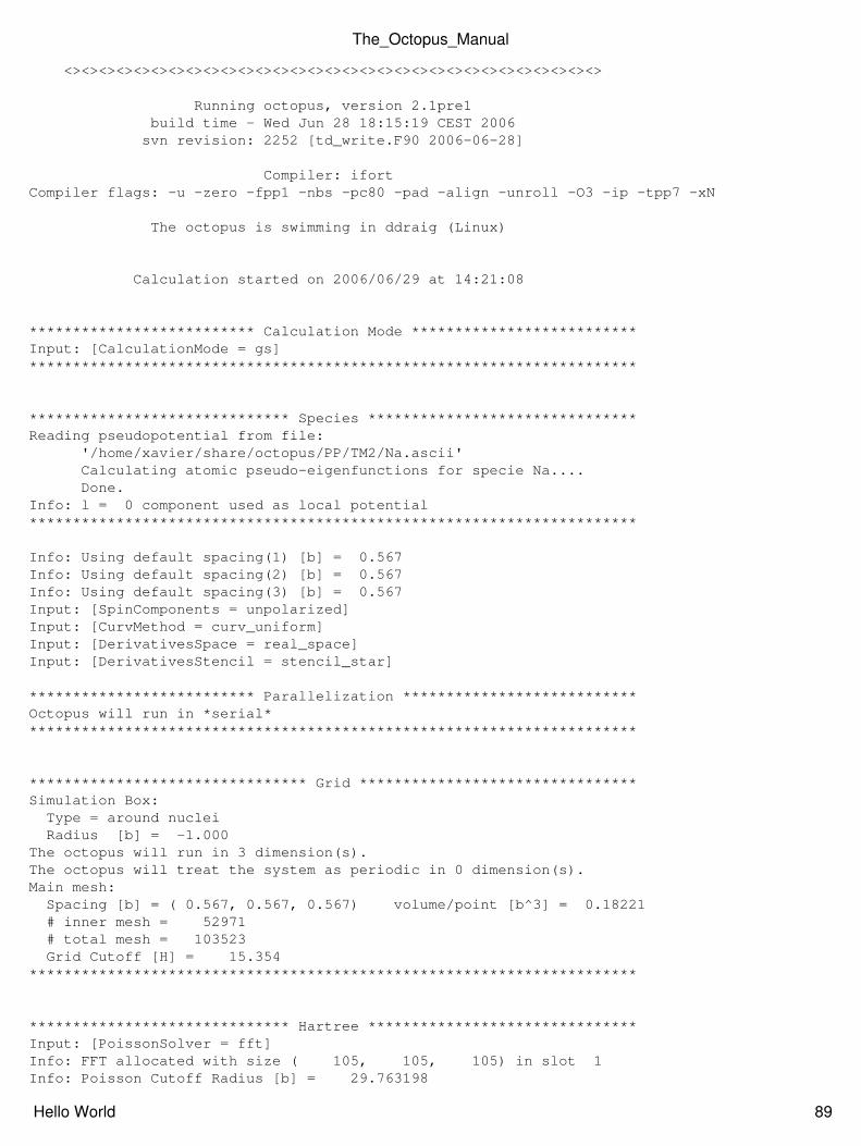
<><><><><><><><><><><><><><><><><><><><><><><><><><><><><><><>
Running octopus, version 2.1pre1 build time - Wed Jun 28 18:15:19 CEST 2006 svn revision: 2252 [td_write.F90 2006-06-28]
Compiler: ifortCompiler flags: -u -zero -fpp1 -nbs -pc80 -pad -align -unroll -O3 -ip -tpp7 -xN
The octopus is swimming in ddraig (Linux)
Calculation started on 2006/06/29 at 14:21:08
************************** Calculation Mode **************************Input: [CalculationMode = gs]**********************************************************************
****************************** Species *******************************Reading pseudopotential from file: '/home/xavier/share/octopus/PP/TM2/Na.ascii' Calculating atomic pseudo-eigenfunctions for specie Na.... Done.Info: l = 0 component used as local potential**********************************************************************
Info: Using default spacing(1) [b] = 0.567Info: Using default spacing(2) [b] = 0.567Info: Using default spacing(3) [b] = 0.567Input: [SpinComponents = unpolarized]Input: [CurvMethod = curv_uniform]Input: [DerivativesSpace = real_space]Input: [DerivativesStencil = stencil_star]
************************** Parallelization ***************************Octopus will run in *serial***********************************************************************
******************************** Grid ********************************Simulation Box: Type = around nuclei Radius [b] = -1.000The octopus will run in 3 dimension(s).The octopus will treat the system as periodic in 0 dimension(s).Main mesh: Spacing [b] = ( 0.567, 0.567, 0.567) volume/point [b^3] = 0.18221 # inner mesh = 52971 # total mesh = 103523 Grid Cutoff [H] = 15.354**********************************************************************
****************************** Hartree *******************************Input: [PoissonSolver = fft]Info: FFT allocated with size ( 105, 105, 105) in slot 1Info: Poisson Cutoff Radius [b] = 29.763198
The_Octopus_Manual
Hello World 89
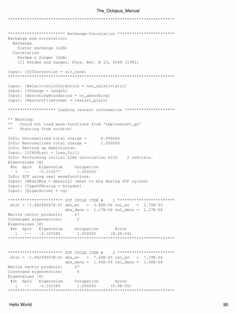
**********************************************************************
************************ Exchange-Correlation ************************Exchange and correlation: Exchange Slater exchange (LDA) Correlation Perdew & Zunger (LDA) [1] Perdew and Zunger, Phys. Rev. B 23, 5048 (1981)
Input: [SICCorrection = sic_none]**********************************************************************
Input: [RelativisticCorrection = non_relativistic]Input: [TDGauge = length]Input: [AbsorbingBoundaries = no_absorbing]Input: [RestartFileFormat = restart_plain]
******************** Loading restart information *********************
** Warning:** Could not load wave-functions from 'tmp/restart_gs'** Starting from scratch!
Info: Unnormalized total charge = 0.999665Info: Renormalized total charge = 1.000000Info: Setting up Hamiltonian.Input: [LCAOStart = lcao_full]Info: Performing initial LCAO calculation with 2 orbitals.Eigenvalues [H] #st Spin Eigenvalue Occupation 1 -- -0.103077 1.000000Info: SCF using real wavefunctions.Input: [What2Mix = density] (what to mix during SCF cycles)Input: [TypeOfMixing = broyden]Input: [EigenSolver = cg]
*********************** SCF CYCLE ITER # 1 ************************ etot = -1.84248567E-01 abs_ev = 3.88E-04 rel_ev = 3.75E-03 abs_dens = 1.17E-04 rel_dens = 1.17E-04Matrix vector products: 27Converged eigenvectors: 0Eigenvalues [H] #st Spin Eigenvalue Occupation Error 1 -- -0.103465 1.000000 (8.2E-04)**********************************************************************
*********************** SCF CYCLE ITER # 2 ************************ etot = -1.84249567E-01 abs_ev = 7.64E-05 rel_ev = 7.39E-04 abs_dens = 1.40E-04 rel_dens = 1.40E-04Matrix vector products: 27Converged eigenvectors: 0Eigenvalues [H] #st Spin Eigenvalue Occupation Error 1 -- -0.103389 1.000000 (5.8E-05)**********************************************************************
The_Octopus_Manual
Hello World 90
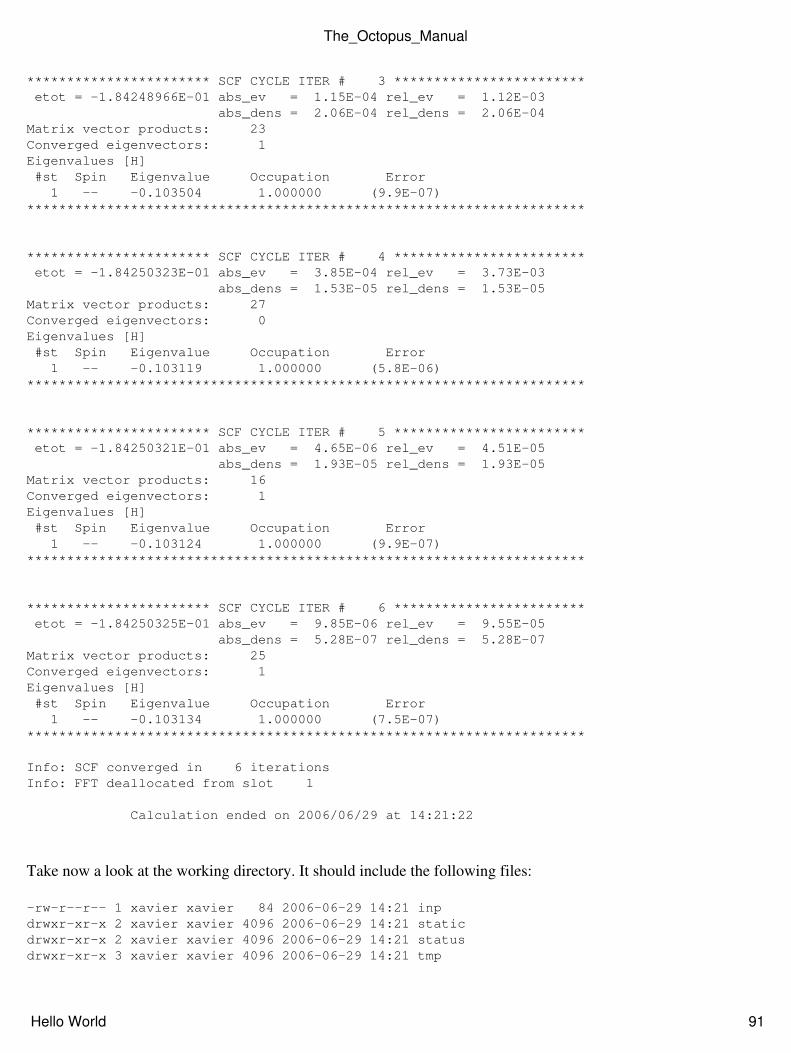
*********************** SCF CYCLE ITER # 3 ************************ etot = -1.84248966E-01 abs_ev = 1.15E-04 rel_ev = 1.12E-03 abs_dens = 2.06E-04 rel_dens = 2.06E-04Matrix vector products: 23Converged eigenvectors: 1Eigenvalues [H] #st Spin Eigenvalue Occupation Error 1 -- -0.103504 1.000000 (9.9E-07)**********************************************************************
*********************** SCF CYCLE ITER # 4 ************************ etot = -1.84250323E-01 abs_ev = 3.85E-04 rel_ev = 3.73E-03 abs_dens = 1.53E-05 rel_dens = 1.53E-05Matrix vector products: 27Converged eigenvectors: 0Eigenvalues [H] #st Spin Eigenvalue Occupation Error 1 -- -0.103119 1.000000 (5.8E-06)**********************************************************************
*********************** SCF CYCLE ITER # 5 ************************ etot = -1.84250321E-01 abs_ev = 4.65E-06 rel_ev = 4.51E-05 abs_dens = 1.93E-05 rel_dens = 1.93E-05Matrix vector products: 16Converged eigenvectors: 1Eigenvalues [H] #st Spin Eigenvalue Occupation Error 1 -- -0.103124 1.000000 (9.9E-07)**********************************************************************
*********************** SCF CYCLE ITER # 6 ************************ etot = -1.84250325E-01 abs_ev = 9.85E-06 rel_ev = 9.55E-05 abs_dens = 5.28E-07 rel_dens = 5.28E-07Matrix vector products: 25Converged eigenvectors: 1Eigenvalues [H] #st Spin Eigenvalue Occupation Error 1 -- -0.103134 1.000000 (7.5E-07)**********************************************************************
Info: SCF converged in 6 iterationsInfo: FFT deallocated from slot 1
Calculation ended on 2006/06/29 at 14:21:22
Take now a look at the working directory. It should include the following files:
-rw-r--r-- 1 xavier xavier 84 2006-06-29 14:21 inp drwxr-xr-x 2 xavier xavier 4096 2006-06-29 14:21 staticdrwxr-xr-x 2 xavier xavier 4096 2006-06-29 14:21 statusdrwxr-xr-x 3 xavier xavier 4096 2006-06-29 14:21 tmp
The_Octopus_Manual
Hello World 91
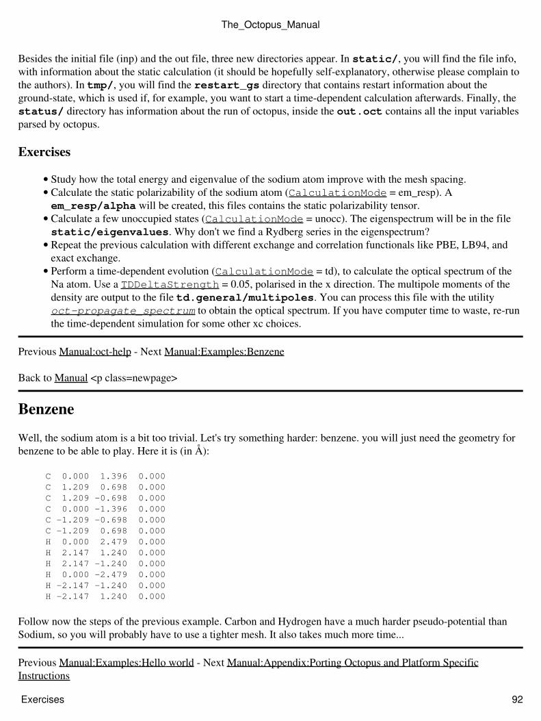
Besides the initial file (inp) and the out file, three new directories appear. In static/, you will find the file info,with information about the static calculation (it should be hopefully self-explanatory, otherwise please complain tothe authors). In tmp/, you will find the restart_gs directory that contains restart information about theground-state, which is used if, for example, you want to start a time-dependent calculation afterwards. Finally, thestatus/ directory has information about the run of octopus, inside the out.oct contains all the input variablesparsed by octopus.
Exercises
Study how the total energy and eigenvalue of the sodium atom improve with the mesh spacing.• Calculate the static polarizability of the sodium atom (CalculationMode = em_resp). Aem_resp/alpha will be created, this files contains the static polarizability tensor.
•
Calculate a few unoccupied states (CalculationMode = unocc). The eigenspectrum will be in the filestatic/eigenvalues. Why don't we find a Rydberg series in the eigenspectrum?
•
Repeat the previous calculation with different exchange and correlation functionals like PBE, LB94, andexact exchange.
•
Perform a time-dependent evolution (CalculationMode = td), to calculate the optical spectrum of theNa atom. Use a TDDeltaStrength = 0.05, polarised in the x direction. The multipole moments of thedensity are output to the file td.general/multipoles. You can process this file with the utility oct-propagate_spectrum to obtain the optical spectrum. If you have computer time to waste, re-runthe time-dependent simulation for some other xc choices.
•
Previous Manual:oct-help - Next Manual:Examples:Benzene
Back to Manual <p class=newpage>
Benzene
Well, the sodium atom is a bit too trivial. Let's try something harder: benzene. you will just need the geometry forbenzene to be able to play. Here it is (in Å):
C 0.000 1.396 0.000 C 1.209 0.698 0.000 C 1.209 -0.698 0.000 C 0.000 -1.396 0.000 C -1.209 -0.698 0.000 C -1.209 0.698 0.000 H 0.000 2.479 0.000 H 2.147 1.240 0.000 H 2.147 -1.240 0.000 H 0.000 -2.479 0.000 H -2.147 -1.240 0.000 H -2.147 1.240 0.000
Follow now the steps of the previous example. Carbon and Hydrogen have a much harder pseudo-potential thanSodium, so you will probably have to use a tighter mesh. It also takes much more time...
Previous Manual:Examples:Hello world - Next Manual:Appendix:Porting Octopus and Platform SpecificInstructions
The_Octopus_Manual
Exercises 92
Back to Manual <p class=newpage>
Variables<p class=newpage>
td_occup
When performing a time-dependent run, the variable TDOutput may be set to TDOutput =td_occup, which,according to the manual, outputs the projections of the time-dependent Kohn-Sham wavefunctions onto the static(zero-time) wavefunctions to the file td.general/projections.XXX.
This will fail if you are running Octopus "parallel in states", since information is dispersed over many nodes. Youmay run in serial mode or "parallel in domains".
In my experience, Octopus writes these projections to the file td.general/projections, in the format:
Iteration Time Re{Projection 1,1} Im{Projection 1,1} Re{Projection 1,2} ...
Rather than the different timesteps getting separate files as described in the manual, after "OutputEvery"timesteps, the projections (preceded by the iteration number and time) will be appended to the filetd.general/projections.
Projections are a complex number, with real and imaginary parts between -1 and 1. Even if the ground state wavefunctions are real, the time evolved ones are complex.
Previous Manual - Next Manual
Back to Manual <p class=newpage>
Appendix<p class=newpage>
Appendix: Updating to a new version
This page lists the issues that may appear when updating to a new version of Octopus and how to solve them.
Octopus 4.1
Installation
This version requires libxc 2.0.0 or higher, so it might be necessary to update libxc before installing Octopus.
The_Octopus_Manual
Appendix 93
Restart files
Casida restart file is incompatible with that generated by version 4.0. The new format avoids problems withrestarting with a different number of states.
Octopus 4.0
Installation
Libxc is now an independent library. To compile Octopus 4.0.0 you will have to compile libxc 1.1.0 first.These are the short instructions to compile it (we assume that libxc will be installed in $DIR, this can be thesame directory where Octopus is going to be installed):
•
tar -xvzf libxc-1.1.0.tar.gzcd libxc-1.1.0 ./configure --prefix=$DIRmakemake install
Now, when configuring Octopus pass the option --with-libxc-prefix=$DIR.
The configure option for the location of netcdf and etsf_io are --with-netcdf-prefix and--with-etsf-io-prefix.
•
Variables
TDEvolutionMethod is now called TDPropagator.•
Utilities
oct-cross_section was renamed to oct-propagation_spectrum.• oct-broad was renamed to oct-casida_spectrum.• The format for oct-help has changed. Now -s is used instead of search, -p instead of show, and -linstead of list.
•
Octopus 3.0
Input variables
Some variables changed name or change format. If an obsolete variable is found, Octopus will stop and will tellyou the variable that replaces it.
Units, UnitsInput and UnitsOutput now take a named option as argument instead of a string. So•
Units = "eVA"
should be replaced by
Units = ev_angstrom
. The code will stop if the old format is encountered.
The_Octopus_Manual
Restart files 94
XFunctional and CFunctional were replaced by XCFunctional, for example•
XFunctional = lda_xCFunctional = lda_c_vwn
must be replaced with
XCFunctional = lda_x + lda_c_vwn
.
TDLasers was replaced by TDExternalFields.• Some options for CalculationMode were renamed.•
Output directories
Some directories in octopus output were renamed, restart files now are stored under restart/ instead of tmp/.Files previously found under status/ are now located in exec/.
Restart file format
Octopus writes restart files in a binary format, this format has been updated and improved. As a result Octopus isno longer able to restart automatically the calculation of a run performed with older versions.
Recovering old restart files
If you really need to recover your old restart files, first you have to generate NetCDF restart files with your oldversion of Octopus. Then you will have to rename the tmp/ directory to restart/ and remove the restart_prefix from its subdirectories, for example tmp/restart_gs/ now should be called restart/gs/.
Now you can run Octopus 3.0 and it will find your restart information. <p class=newpage>
Appendix: Building from scratch
Compiling Octopus on some systems might be difficult, this is mainly because some libraries are required and theyhave to be all compiled with same Fortran compiler. This is a guide on how to compile Octopus and the requiredlibraries starting from scratch (a Fortran compiler is required) in a standard Unix system.
NOTE: This page should be considered a last resort. On most systems you will be able to install many ofthese dependencies from a package manager or other pre-built binaries, which will save you a lot of effort.
Prerequisites
You will need the following:
A standard Unix/Linux system, where you want to install Octopus.• A basic knowledge on how to use the system (manage files, edit text files, extract tar archives, etc.).• A directory where we will install the created binaries, this can be a specially created directory or even your$HOME. From now, we will assume that the directory is <basedir>, whenever it appears you should
•
The_Octopus_Manual
Input variables 95
replace it with the actual directory you are using. Note that the files that you will download and thedirectories with the sources, including the ones of Octopus, don't need to be placed in this directory.A working C compiler, gcc is the ideal choice for x86/x86_64 systems. For other platforms you might wantto choose a compiler that produces more optimized code. We will assume that the command to run thecompiler is <cc>.
•
A working Fortran 95 compiler, if you don't have one you can probably get gfortran or g95. We willassume that the command to run the Fortran compiler is <fc>.
•
If you are compiling for a dual 32/64 bits architecture, it is a good idea to tell the compilers explicitly whattype of binaries you want, many problems are caused by unadvertedly mixing 32 and 64 bits code. ForOctopus normally you will want a 64 bits binary (-m64 flag in most compilers). Since this flag should bepassed always we recommend you to include it in the compiler command used in this guide (sometimesoptimization flags are left out), so for example <cc> could be gcc -m64.
•
Compiler flags
Since probably you want Octopus to run fast, you will probably would to set optimization flags for both the C andFortran compilers on your system (at least -O3). In general Octopus should run fine with aggressive optimizationoptions. We will assume now that you have found a set of flags for <cc> and <fc>, we will call them <cflags>and <fcflags>. For example <cflags> could be -O3 -march=native.
Note: if <cc>, <fc>, <cflags> or <fcflags> contain spaces you should not enclose them in "". We will putthe "" explicitly when it is necessary.
Compilation of libraries
First we will compile and install the libraries required by Octopus.
BLAS
The first library we will compile is blas. We will use the generic reference implementation, this version is nothighly optimized but it is free software and simple to install. So after you have a working version of Octopus youmay want to use a more optimized blas implementation as libgoto, ATLAS, MKL, ACML, ESSL, etc.
Download the package from the netlib site: http://www.netlib.org/blas/blas.tgz• Extract the package and enter into the newly created BLAS directory.• Edit the make.inc file and modify the definition of the fortran compiler that now should be:•
FORTRAN = <fc>OPTS = <fcflags>DRVOPTS = $(OPTS)NOOPT =LOADER = <fc>LOADOPTS =
Now type make to compile, this will take a while.• One compilation is finished, create the directory <basedir>/lib•
mkdir <basedir>/lib
The_Octopus_Manual
Prerequisites 96
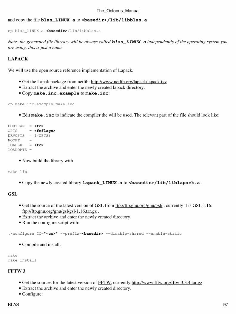
and copy the file blas_LINUX.a to <basedir>/lib/libblas.a
cp blas_LINUX.a <basedir>/lib/libblas.a
Note: the generated file librrary will be always called blas_LINUX.a independently of the operating system youare using, this is just a name.
LAPACK
We will use the open source reference implementation of Lapack.
Get the Lapak package from netlib: http://www.netlib.org/lapack/lapack.tgz• Extract the archive and enter the newly created lapack directory.• Copy make.inc.example to make.inc:•
cp make.inc.example make.inc
Edit make.inc to indicate the compiler the will be used. The relevant part of the file should look like:•
FORTRAN = <fc>OPTS = <fcflags>DRVOPTS = $(OPTS)NOOPT =LOADER = <fc>LOADOPTS =
Now build the library with•
make lib
Copy the newly created library lapack_LINUX.a to <basedir>/lib/liblapack.a .•
GSL
Get the source of the latest version of GSL from ftp://ftp.gnu.org/gnu/gsl/ , currently it is GSL 1.16:ftp://ftp.gnu.org/gnu/gsl/gsl-1.16.tar.gz .
•
Extract the archive and enter the newly created directory.• Run the configure script with:•
./configure CC="<cc>" --prefix=<basedir> --disable-shared --enable-static
Compile and install:•
makemake install
FFTW 3
Get the sources for the latest version of FFTW, currently http://www.fftw.org/fftw-3.3.4.tar.gz .• Extract the archive and enter the newly created directory.• Configure:•
The_Octopus_Manual
BLAS 97
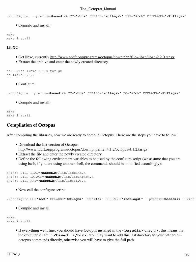
./configure --prefix=<basedir> CC="<cc>" CFLAGS="<cflags>" F77="<fc>" F77FLAGS="<fcflags>"
Compile and install:•
makemake install
LibXC
Get libxc, currently http://www.tddft.org/programs/octopus/down.php?file=libxc/libxc-2.2.0.tar.gz .• Extract the archive and enter the newly created directory.•
tar -xvzf libxc-2.2.0.tar.gzcd libxc-2.2.0
Configure:•
./configure --prefix=<basedir> CC="<cc>" CFLAGS="<cflags>" FC="<fc>" FCFLAGS="<fcflags>"
Compile and install:•
makemake install
Compilation of Octopus
After compiling the libraries, now we are ready to compile Octopus. These are the steps you have to follow:
Download the last version of Octopus:http://www.tddft.org/programs/octopus/down.php?file=4.1.2/octopus-4.1.2.tar.gz
•
Extract the file and enter the newly created directory.• Define the following environment variables to be used by the configure script (we assume that you areusing bash, if you are using another shell, the commands should be modified accordingly):
•
export LIBS_BLAS=<basedir>/lib/libblas.aexport LIBS_LAPACK=<basedir>/lib/liblapack.aexport LIBS_FFT=<basedir>/lib/libfftw3.a
Now call the configure script:•
./configure CC="<cc>" CFLAGS="<cflags>" FC="<fc>" FCFLAGS="<fcflags>" --prefix=<basedir> --with-gsl-prefix=<basedir> --with-libxc-prefix=<basedir>
Compile and install•
makemake install
If everything went fine, you should have Octopus installed in the <basedir> directory, this means thatthe executables are in <basedir>/bin/. You may want to add this last directory to your path to runoctopus commands directly, otherwise you will have to give the full path.
•
The_Octopus_Manual
FFTW 3 98
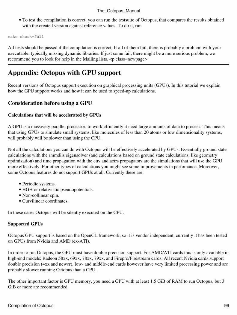
To test the compilation is correct, you can run the testsuite of Octopus, that compares the results obtainedwith the created version against reference values. To do it, run
•
make check-full
All tests should be passed if the compilation is correct. If all of them fail, there is probably a problem with yourexecutable, typically missing dynamic libraries. If just some fail, there might be a more serious problem, werecommend you to look for help in the Mailing lists. <p class=newpage>
Appendix: Octopus with GPU support
Recent versions of Octopus support execution on graphical processing units (GPUs). In this tutorial we explainhow the GPU support works and how it can be used to speed-up calculations.
Consideration before using a GPU
Calculations that will be accelerated by GPUs
A GPU is a massively parallel processor, to work efficiently it need large amounts of data to process. This meansthat using GPUs to simulate small systems, like molecules of less than 20 atoms or low dimensionality systems,will probably will be slower than using the CPU.
Not all the calculations you can do with Octopus will be effectively accelerated by GPUs. Essentially ground statecalculations with the rmmdiis eigensolver (and calculations based on ground state calculations, like geometryoptimization) and time propagation with the etrs and aetrs propagators are the simulations that will use the GPUmore effectively. For other types of calculations you might see some improvements in perfomance. Moreover,some Octopus features do not support GPUs at all. Currently these are:
Periodic systems.• HGH or relativistic pseudopotentials.• Non-collinear spin.• Curvilinear coordinates.•
In these cases Octopus will be silently executed on the CPU.
Supported GPUs
Octopus GPU support is based on the OpenCL framework, so it is vendor independent, currently it has been testedon GPUs from Nvidia and AMD (ex-ATI).
In order to run Octopus, the GPU must have double precision support. For AMD/ATI cards this is only available inhigh-end models: Radeon 58xx, 69xx, 78xx, 79xx, and Firepro/Firestream cards. All recent Nvidia cards supportdouble precision (4xx and newer), low- and middle-end cards however have very limited processing power and areprobably slower running Octopus than a CPU.
The other important factor is GPU memory, you need a GPU with at least 1.5 GiB of RAM to run Octopus, but 3GiB or more are recommended.
The_Octopus_Manual
Compilation of Octopus 99
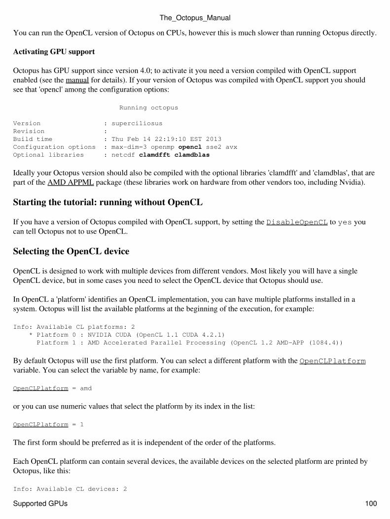
You can run the OpenCL version of Octopus on CPUs, however this is much slower than running Octopus directly.
Activating GPU support
Octopus has GPU support since version 4.0; to activate it you need a version compiled with OpenCL supportenabled (see the manual for details). If your version of Octopus was compiled with OpenCL support you shouldsee that 'opencl' among the configuration options:
Running octopus
Version : superciliosusRevision :Build time : Thu Feb 14 22:19:10 EST 2013Configuration options : max-dim=3 openmp opencl sse2 avxOptional libraries : netcdf clamdfft clamdblas
Ideally your Octopus version should also be compiled with the optional libraries 'clamdfft' and 'clamdblas', that arepart of the AMD APPML package (these libraries work on hardware from other vendors too, including Nvidia).
Starting the tutorial: running without OpenCL
If you have a version of Octopus compiled with OpenCL support, by setting the DisableOpenCL to yes youcan tell Octopus not to use OpenCL.
Selecting the OpenCL device
OpenCL is designed to work with multiple devices from different vendors. Most likely you will have a singleOpenCL device, but in some cases you need to select the OpenCL device that Octopus should use.
In OpenCL a 'platform' identifies an OpenCL implementation, you can have multiple platforms installed in asystem. Octopus will list the available platforms at the beginning of the execution, for example:
Info: Available CL platforms: 2 * Platform 0 : NVIDIA CUDA (OpenCL 1.1 CUDA 4.2.1) Platform 1 : AMD Accelerated Parallel Processing (OpenCL 1.2 AMD-APP (1084.4))
By default Octopus will use the first platform. You can select a different platform with the OpenCLPlatformvariable. You can select the variable by name, for example:
OpenCLPlatform = amd
or you can use numeric values that select the platform by its index in the list:
OpenCLPlatform = 1
The first form should be preferred as it is independent of the order of the platforms.
Each OpenCL platform can contain several devices, the available devices on the selected platform are printed byOctopus, like this:
Info: Available CL devices: 2
The_Octopus_Manual
Supported GPUs 100
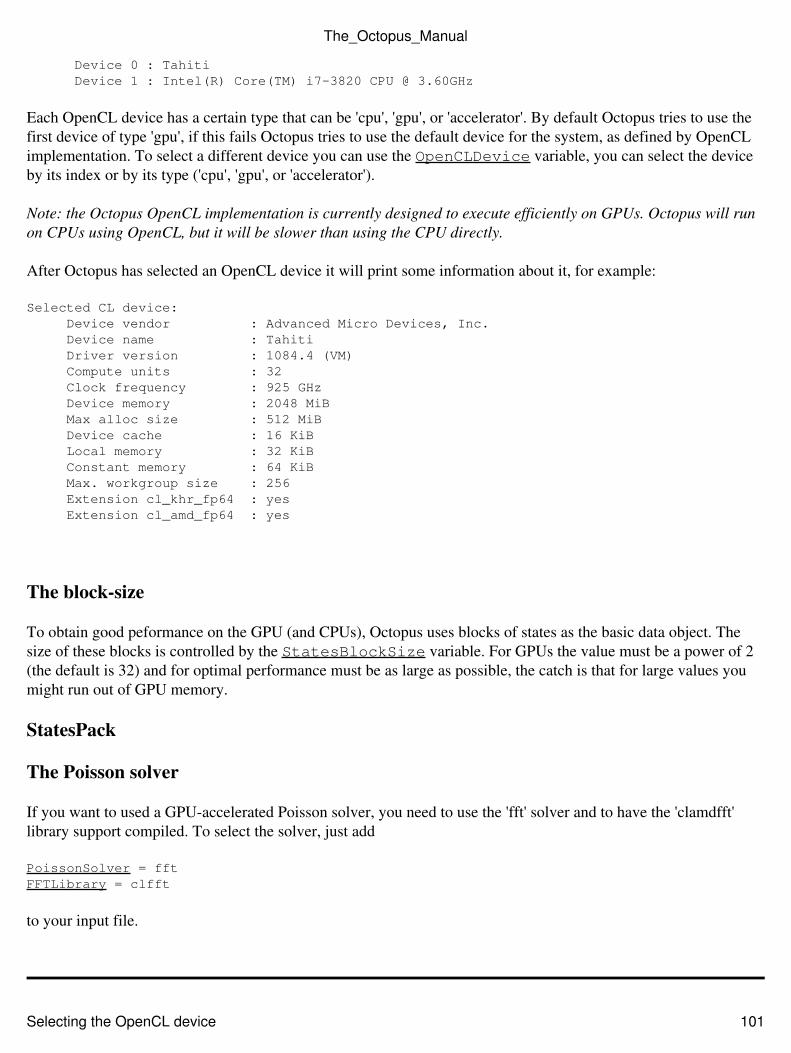
Device 0 : Tahiti Device 1 : Intel(R) Core(TM) i7-3820 CPU @ 3.60GHz
Each OpenCL device has a certain type that can be 'cpu', 'gpu', or 'accelerator'. By default Octopus tries to use thefirst device of type 'gpu', if this fails Octopus tries to use the default device for the system, as defined by OpenCLimplementation. To select a different device you can use the OpenCLDevice variable, you can select the deviceby its index or by its type ('cpu', 'gpu', or 'accelerator').
Note: the Octopus OpenCL implementation is currently designed to execute efficiently on GPUs. Octopus will runon CPUs using OpenCL, but it will be slower than using the CPU directly.
After Octopus has selected an OpenCL device it will print some information about it, for example:
Selected CL device: Device vendor : Advanced Micro Devices, Inc. Device name : Tahiti Driver version : 1084.4 (VM) Compute units : 32 Clock frequency : 925 GHz Device memory : 2048 MiB Max alloc size : 512 MiB Device cache : 16 KiB Local memory : 32 KiB Constant memory : 64 KiB Max. workgroup size : 256 Extension cl_khr_fp64 : yes Extension cl_amd_fp64 : yes
The block-size
To obtain good peformance on the GPU (and CPUs), Octopus uses blocks of states as the basic data object. Thesize of these blocks is controlled by the StatesBlockSize variable. For GPUs the value must be a power of 2(the default is 32) and for optimal performance must be as large as possible, the catch is that for large values youmight run out of GPU memory.
StatesPack
The Poisson solver
If you want to used a GPU-accelerated Poisson solver, you need to use the 'fft' solver and to have the 'clamdfft'library support compiled. To select the solver, just add
PoissonSolver = fftFFTLibrary = clfft
to your input file.
The_Octopus_Manual
Selecting the OpenCL device 101
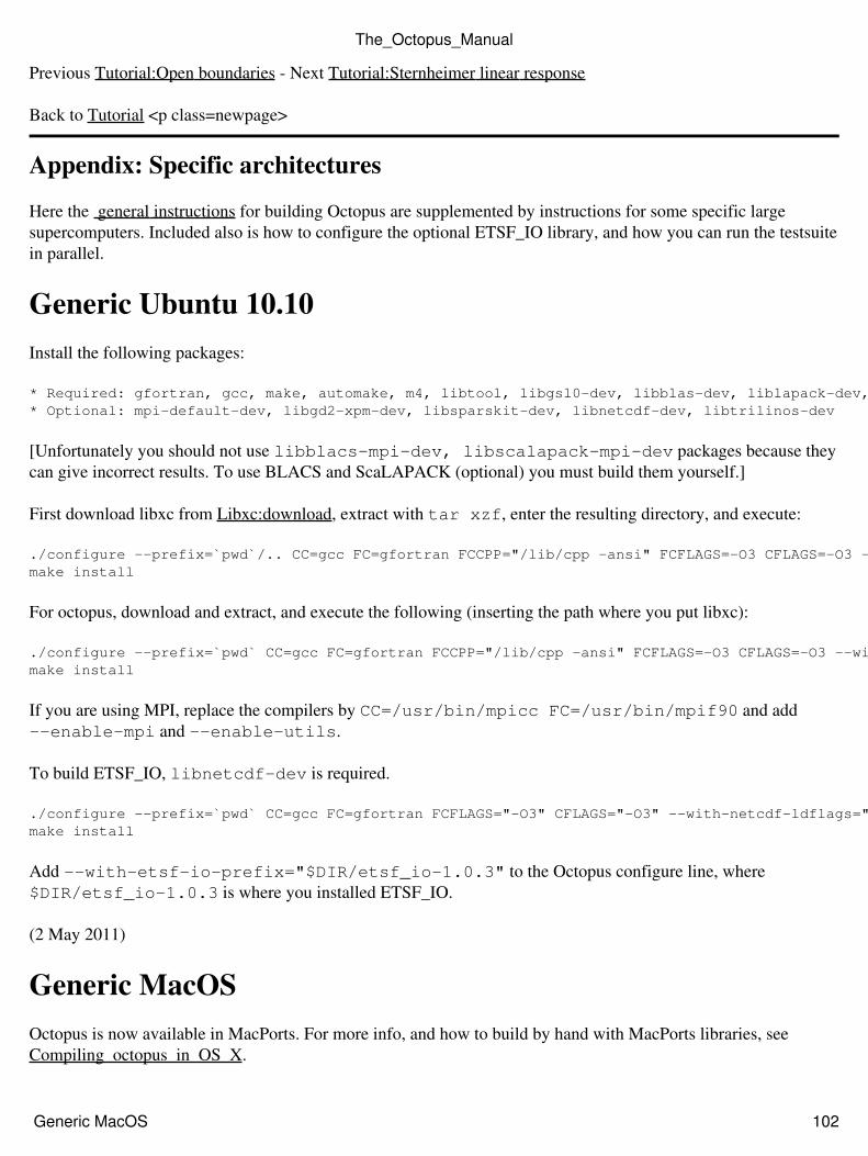
Previous Tutorial:Open boundaries - Next Tutorial:Sternheimer linear response
Back to Tutorial <p class=newpage>
Appendix: Specific architectures
Here the general instructions for building Octopus are supplemented by instructions for some specific largesupercomputers. Included also is how to configure the optional ETSF_IO library, and how you can run the testsuitein parallel.
Generic Ubuntu 10.10Install the following packages:
* Required: gfortran, gcc, make, automake, m4, libtool, libgsl0-dev, libblas-dev, liblapack-dev, libfftw3-dev* Optional: mpi-default-dev, libgd2-xpm-dev, libsparskit-dev, libnetcdf-dev, libtrilinos-dev
[Unfortunately you should not use libblacs-mpi-dev, libscalapack-mpi-dev packages because theycan give incorrect results. To use BLACS and ScaLAPACK (optional) you must build them yourself.]
First download libxc from Libxc:download, extract with tar xzf, enter the resulting directory, and execute:
./configure --prefix=`pwd`/.. CC=gcc FC=gfortran FCCPP="/lib/cpp -ansi" FCFLAGS=-O3 CFLAGS=-O3 --disable-sharedmake install
For octopus, download and extract, and execute the following (inserting the path where you put libxc):
./configure --prefix=`pwd` CC=gcc FC=gfortran FCCPP="/lib/cpp -ansi" FCFLAGS=-O3 CFLAGS=-O3 --with-libxc-prefix=LIBXC_PATH --enable-newuoamake install
If you are using MPI, replace the compilers by CC=/usr/bin/mpicc FC=/usr/bin/mpif90 and add--enable-mpi and --enable-utils.
To build ETSF_IO, libnetcdf-dev is required.
./configure --prefix=`pwd` CC=gcc FC=gfortran FCFLAGS="-O3" CFLAGS="-O3" --with-netcdf-ldflags="-lnetcdff"make install
Add --with-etsf-io-prefix="$DIR/etsf_io-1.0.3" to the Octopus configure line, where$DIR/etsf_io-1.0.3 is where you installed ETSF_IO.
(2 May 2011)
Generic MacOSOctopus is now available in MacPorts. For more info, and how to build by hand with MacPorts libraries, seeCompiling_octopus_in_OS_X.
The_Octopus_Manual
Generic MacOS 102
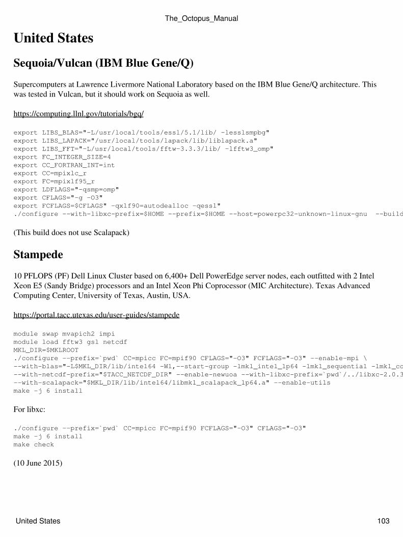
United States
Sequoia/Vulcan (IBM Blue Gene/Q)
Supercomputers at Lawrence Livermore National Laboratory based on the IBM Blue Gene/Q architecture. Thiswas tested in Vulcan, but it should work on Sequoia as well.
https://computing.llnl.gov/tutorials/bgq/
export LIBS_BLAS="-L/usr/local/tools/essl/5.1/lib/ -lesslsmpbg"export LIBS_LAPACK="/usr/local/tools/lapack/lib/liblapack.a"export LIBS_FFT="-L/usr/local/tools/fftw-3.3.3/lib/ -lfftw3_omp"export FC_INTEGER_SIZE=4export CC_FORTRAN_INT=intexport CC=mpixlc_rexport FC=mpixlf95_rexport LDFLAGS="-qsmp=omp"export CFLAGS="-g -O3"export FCFLAGS=$CFLAGS" -qxlf90=autodealloc -qessl"./configure --with-libxc-prefix=$HOME --prefix=$HOME --host=powerpc32-unknown-linux-gnu --build=powerpc64-unknown-linux-gnu --with-gsl-prefix=$HOME --enable-openmp --enable-mpi
(This build does not use Scalapack)
Stampede
10 PFLOPS (PF) Dell Linux Cluster based on 6,400+ Dell PowerEdge server nodes, each outfitted with 2 IntelXeon E5 (Sandy Bridge) processors and an Intel Xeon Phi Coprocessor (MIC Architecture). Texas AdvancedComputing Center, University of Texas, Austin, USA.
https://portal.tacc.utexas.edu/user-guides/stampede
module swap mvapich2 impimodule load fftw3 gsl netcdfMKL_DIR=$MKLROOT./configure --prefix=`pwd` CC=mpicc FC=mpif90 CFLAGS="-O3" FCFLAGS="-O3" --enable-mpi \--with-blas="-L$MKL_DIR/lib/intel64 -Wl,--start-group -lmkl_intel_lp64 -lmkl_sequential -lmkl_core -Wl,--end-group -lpthread" --with-fft-lib="-L$TACC_FFTW3_LIB -lfftw3" \--with-netcdf-prefix="$TACC_NETCDF_DIR" --enable-newuoa --with-libxc-prefix=`pwd`/../libxc-2.0.3 --with-blacs="$MKL_DIR/lib/intel64/libmkl_blacs_intelmpi_lp64.a" \--with-scalapack="$MKL_DIR/lib/intel64/libmkl_scalapack_lp64.a" --enable-utilsmake -j 6 install
For libxc:
./configure --prefix=`pwd` CC=mpicc FC=mpif90 FCFLAGS="-O3" CFLAGS="-O3"make -j 6 installmake check
(10 June 2015)
The_Octopus_Manual
United States 103
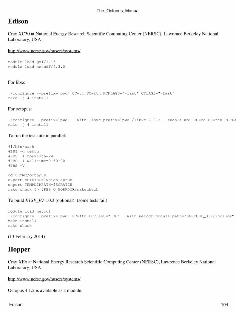
Edison
Cray XC30 at National Energy Research Scientific Computing Center (NERSC), Lawrence Berkeley NationalLaboratory, USA
http://www.nersc.gov/nusers/systems/
module load gsl/1.15module load netcdf/4.3.0
For libxc:
./configure --prefix=`pwd` CC=cc FC=ftn FCFLAGS="-fast" CFLAGS="-fast"make -j 4 install
For octopus:
./configure --prefix=`pwd` --with-libxc-prefix=`pwd`/libxc-2.0.3 --enable-mpi CC=cc FC=ftn FCFLAGS="-fast" CFLAGS="-fast" --enable-newuoa --enable-utilsmake -j 4 install
To run the testsuite in parallel:
#!/bin/bash#PBS -q debug#PBS -l mppwidth=24#PBS -l walltime=0:30:00#PBS -V
cd $HOME/octopusexport MPIEXEC=`which aprun`export TEMPDIRPATH=$SCRATCHmake check &> $PBS_O_WORKDIR/makecheck
To build ETSF_IO 1.0.3 (optional): (some tests fail)
module load netcdf./configure --prefix=`pwd` FC=ftn FCFLAGS="-O0" --with-netcdf-module-path="$NETCDF_DIR/include" --with-netcdf-ldflags="-L$NETCDF_DIR/lib -lnetcdf -lnetcdff"make installmake check
(13 February 2014)
Hopper
Cray XE6 at National Energy Research Scientific Computing Center (NERSC), Lawrence Berkeley NationalLaboratory, USA
http://www.nersc.gov/nusers/systems/
Octopus 4.1.2 is available as a module.
The_Octopus_Manual
Edison 104
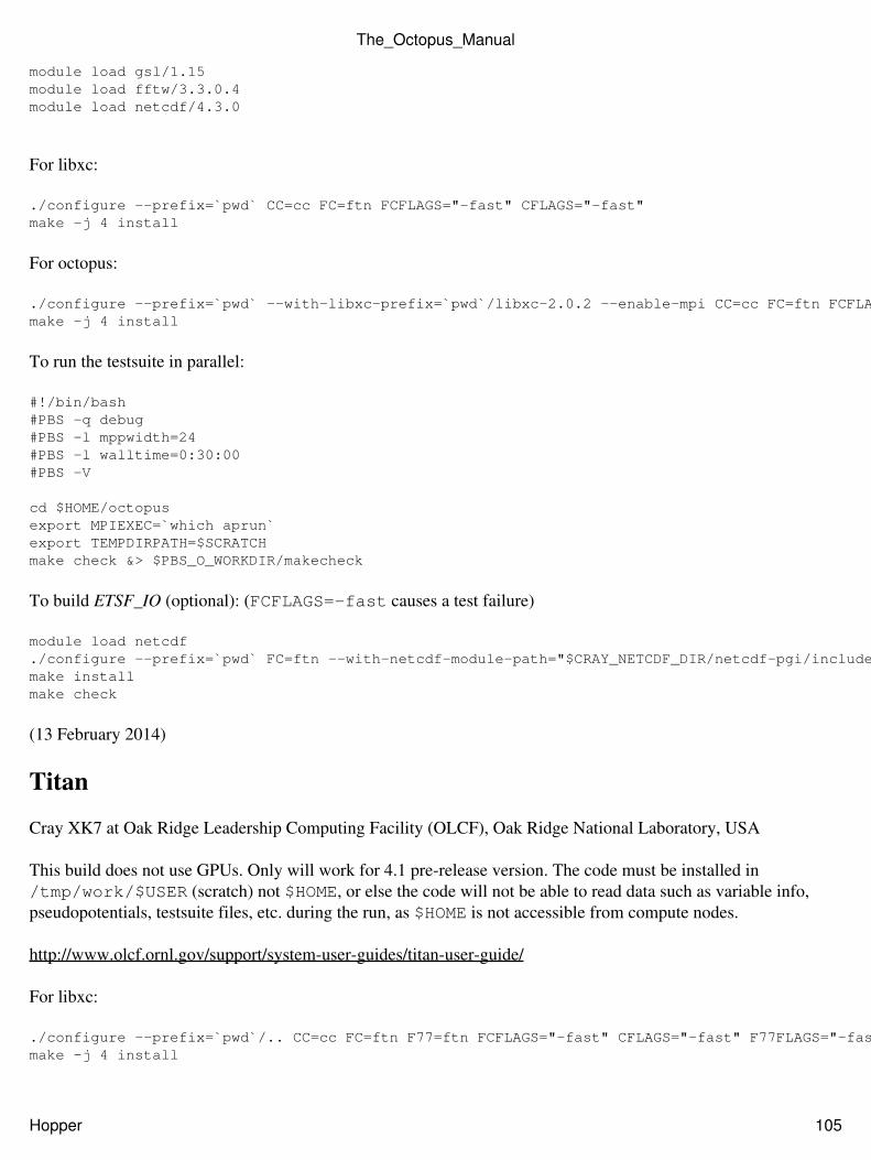
module load gsl/1.15module load fftw/3.3.0.4module load netcdf/4.3.0
For libxc:
./configure --prefix=`pwd` CC=cc FC=ftn FCFLAGS="-fast" CFLAGS="-fast"make -j 4 install
For octopus:
./configure --prefix=`pwd` --with-libxc-prefix=`pwd`/libxc-2.0.2 --enable-mpi CC=cc FC=ftn FCFLAGS="-fast" CFLAGS="-fast" --enable-newuoa --enable-utilsmake -j 4 install
To run the testsuite in parallel:
#!/bin/bash#PBS -q debug#PBS -l mppwidth=24#PBS -l walltime=0:30:00#PBS -V
cd $HOME/octopusexport MPIEXEC=`which aprun`export TEMPDIRPATH=$SCRATCHmake check &> $PBS_O_WORKDIR/makecheck
To build ETSF_IO (optional): (FCFLAGS=-fast causes a test failure)
module load netcdf./configure --prefix=`pwd` FC=ftn --with-netcdf-module-path="$CRAY_NETCDF_DIR/netcdf-pgi/include" --with-netcdf-ldflags="-L$CRAY_NETCDF_DIR/netcdf-pgi/lib"make installmake check
(13 February 2014)
Titan
Cray XK7 at Oak Ridge Leadership Computing Facility (OLCF), Oak Ridge National Laboratory, USA
This build does not use GPUs. Only will work for 4.1 pre-release version. The code must be installed in/tmp/work/$USER (scratch) not $HOME, or else the code will not be able to read data such as variable info,pseudopotentials, testsuite files, etc. during the run, as $HOME is not accessible from compute nodes.
http://www.olcf.ornl.gov/support/system-user-guides/titan-user-guide/
For libxc:
./configure --prefix=`pwd`/.. CC=cc FC=ftn F77=ftn FCFLAGS="-fast" CFLAGS="-fast" F77FLAGS="-fast"make -j 4 install
The_Octopus_Manual
Hopper 105
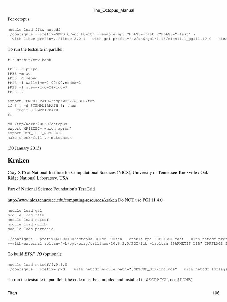
For octopus:
module load fftw netcdf./configure --prefix=$PWD CC=cc FC=ftn --enable-mpi CFLAGS=-fast FCFLAGS="-fast" \--with-libxc-prefix=../libxc-2.0.1 --with-gsl-prefix=/sw/xk6/gsl/1.15/sles11.1_pgi11.10.0 --disable-zdotc-test
To run the testsuite in parallel:
#!/usr/bin/env bash
#PBS -N pulpo#PBS -m ae#PBS -q debug#PBS -l walltime=1:00:00,nodes=2#PBS -l gres=widow2%widow3#PBS -V
export TEMPDIRPATH=/tmp/work/$USER/tmpif [ ! -d $TEMPDIRPATH ]; then mkdir $TEMPDIRPATHfi
cd /tmp/work/$USER/octopusexport MPIEXEC=`which aprun`export OCT_TEST_NJOBS=10make check-full &> makecheck
(30 January 2013)
Kraken
Cray XT5 at National Institute for Computational Sciences (NICS), University of Tennessee-Knoxville / OakRidge National Laboratory, USA
Part of National Science Foundation's TeraGrid
http://www.nics.tennessee.edu/computing-resources/kraken Do NOT use PGI 11.4.0.
module load gslmodule load fftwmodule load netcdfmodule load gdlibmodule load parmetis
./configure --prefix=$SCRATCH/octopus CC=cc FC=ftn --enable-mpi FCFLAGS=-fast --with-netcdf-prefix="$NETCDF_DIR" --enable-newuoa --with-libxc-prefix=`pwd` \ --with-external_zoltan="-L/opt/cray/trilinos/10.6.2.0/PGI/lib -lzoltan $PARMETIS_LIB" CPPFLAGS_ZOLTAN="-I/opt/cray/trilinos/10.6.2.0/PGI/include"
To build ETSF_IO (optional):
module load netcdf/4.0.1.0./configure --prefix=`pwd` --with-netcdf-module-path="$NETCDF_DIR/include" --with-netcdf-ldflags="$POST_LINK_OPTS"
To run the testsuite in parallel: (the code must be compiled and installed in $SCRATCH, not $HOME)
The_Octopus_Manual
Titan 106
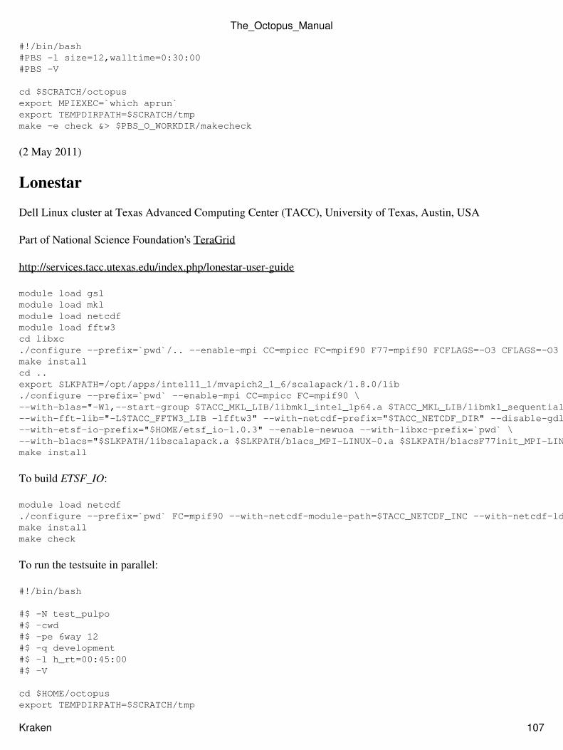
#!/bin/bash#PBS -l size=12,walltime=0:30:00#PBS -V
cd $SCRATCH/octopusexport MPIEXEC=`which aprun`export TEMPDIRPATH=$SCRATCH/tmpmake -e check &> $PBS_O_WORKDIR/makecheck
(2 May 2011)
Lonestar
Dell Linux cluster at Texas Advanced Computing Center (TACC), University of Texas, Austin, USA
Part of National Science Foundation's TeraGrid
http://services.tacc.utexas.edu/index.php/lonestar-user-guide
module load gslmodule load mklmodule load netcdfmodule load fftw3cd libxc./configure --prefix=`pwd`/.. --enable-mpi CC=mpicc FC=mpif90 F77=mpif90 FCFLAGS=-O3 CFLAGS=-O3make installcd ..export SLKPATH=/opt/apps/intel11_1/mvapich2_1_6/scalapack/1.8.0/lib./configure --prefix=`pwd` --enable-mpi CC=mpicc FC=mpif90 \--with-blas="-Wl,--start-group $TACC_MKL_LIB/libmkl_intel_lp64.a $TACC_MKL_LIB/libmkl_sequential.a $TACC_MKL_LIB/libmkl_core.a -Wl,--end-group -lpthread" \--with-fft-lib="-L$TACC_FFTW3_LIB -lfftw3" --with-netcdf-prefix="$TACC_NETCDF_DIR" --disable-gdlib \--with-etsf-io-prefix="$HOME/etsf_io-1.0.3" --enable-newuoa --with-libxc-prefix=`pwd` \--with-blacs="$SLKPATH/libscalapack.a $SLKPATH/blacs_MPI-LINUX-0.a $SLKPATH/blacsF77init_MPI-LINUX-0.a $SLKPATH/blacs_MPI-LINUX-0.a"make install
To build ETSF_IO:
module load netcdf./configure --prefix=`pwd` FC=mpif90 --with-netcdf-module-path=$TACC_NETCDF_INC --with-netcdf-ldflags=-L$TACC_NETCDF_LIB FCFLAGS=-O3make installmake check
To run the testsuite in parallel:
#!/bin/bash
#$ -N test_pulpo#$ -cwd#$ -pe 6way 12#$ -q development#$ -l h_rt=00:45:00#$ -V
cd $HOME/octopusexport TEMPDIRPATH=$SCRATCH/tmp
The_Octopus_Manual
Kraken 107
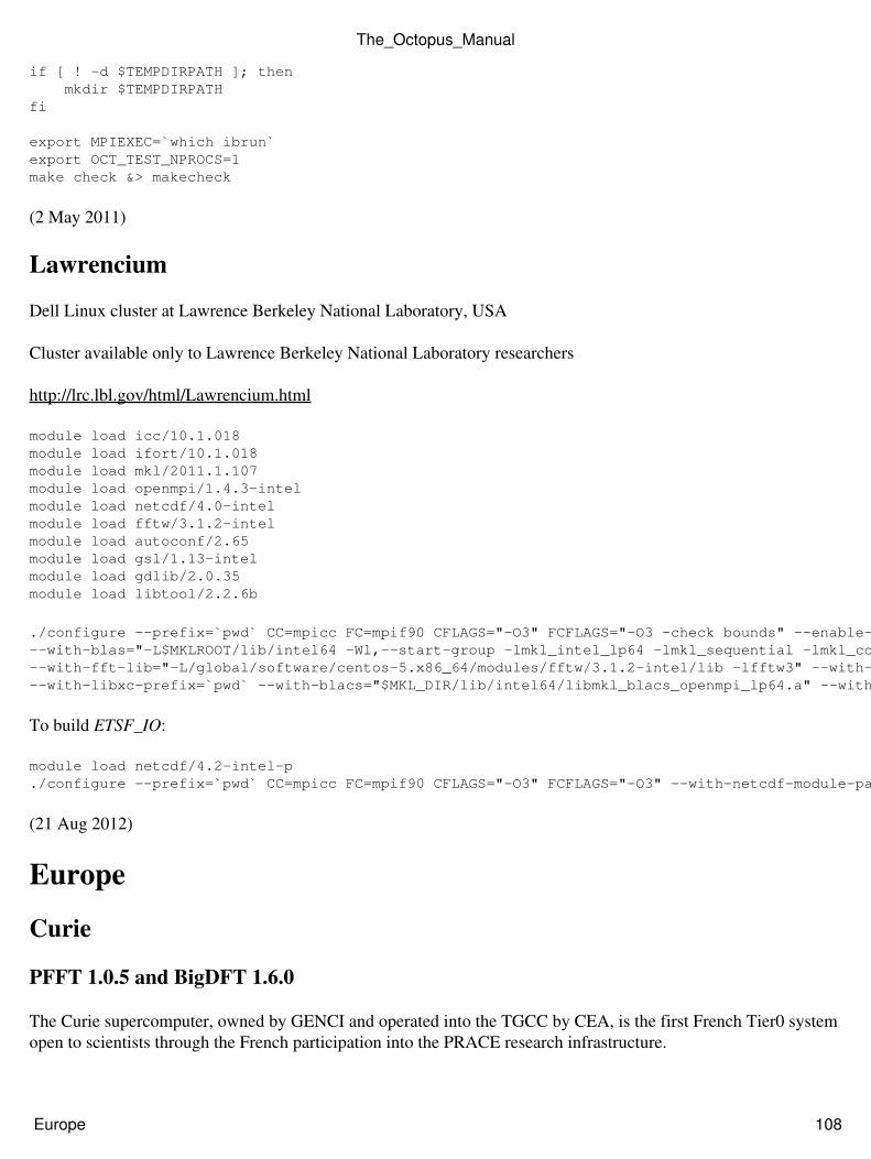
if [ ! -d $TEMPDIRPATH ]; then mkdir $TEMPDIRPATHfi
export MPIEXEC=`which ibrun`export OCT_TEST_NPROCS=1make check &> makecheck
(2 May 2011)
Lawrencium
Dell Linux cluster at Lawrence Berkeley National Laboratory, USA
Cluster available only to Lawrence Berkeley National Laboratory researchers
http://lrc.lbl.gov/html/Lawrencium.html
module load icc/10.1.018module load ifort/10.1.018module load mkl/2011.1.107module load openmpi/1.4.3-intelmodule load netcdf/4.0-intelmodule load fftw/3.1.2-intelmodule load autoconf/2.65module load gsl/1.13-intelmodule load gdlib/2.0.35module load libtool/2.2.6b
./configure --prefix=`pwd` CC=mpicc FC=mpif90 CFLAGS="-O3" FCFLAGS="-O3 -check bounds" --enable-mpi \--with-blas="-L$MKLROOT/lib/intel64 -Wl,--start-group -lmkl_intel_lp64 -lmkl_sequential -lmkl_core -Wl,--end-group -lpthread" \--with-fft-lib="-L/global/software/centos-5.x86_64/modules/fftw/3.1.2-intel/lib -lfftw3" --with-netcdf-prefix="$NETCDF" --with-netcdf-include="$NETCDF/include" --enable-newuoa \--with-libxc-prefix=`pwd` --with-blacs="$MKL_DIR/lib/intel64/libmkl_blacs_openmpi_lp64.a" --with-scalapack="$MKL_DIR/lib/intel64/libmkl_scalapack_lp64.a"
To build ETSF_IO:
module load netcdf/4.2-intel-p./configure --prefix=`pwd` CC=mpicc FC=mpif90 CFLAGS="-O3" FCFLAGS="-O3" --with-netcdf-module-path=$NETCDF_DIR/include/ --with-netcdf-ldflags="-L$NETCDF_DIR/lib/ -lnetcdf"
(21 Aug 2012)
Europe
Curie
PFFT 1.0.5 and BigDFT 1.6.0
The Curie supercomputer, owned by GENCI and operated into the TGCC by CEA, is the first French Tier0 systemopen to scientists through the French participation into the PRACE research infrastructure.
The_Octopus_Manual
Europe 108
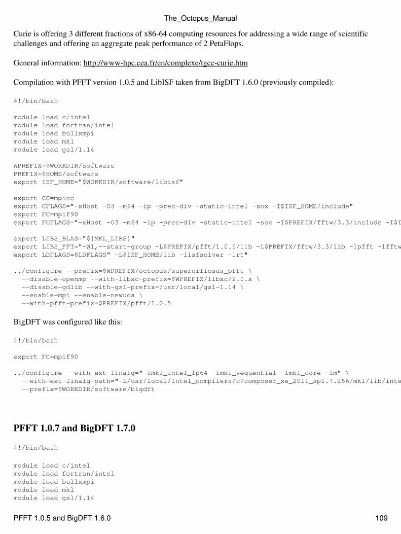
Curie is offering 3 different fractions of x86-64 computing resources for addressing a wide range of scientificchallenges and offering an aggregate peak performance of 2 PetaFlops.
General information: http://www-hpc.cea.fr/en/complexe/tgcc-curie.htm
Compilation with PFFT version 1.0.5 and LibISF taken from BigDFT 1.6.0 (previously compiled):
#!/bin/bash
module load c/intelmodule load fortran/intelmodule load bullxmpimodule load mklmodule load gsl/1.14
WPREFIX=$WORKDIR/softwarePREFIX=$HOME/softwareexport ISF_HOME="$WORKDIR/software/libisf"
export CC=mpiccexport CFLAGS="-xHost -O3 -m64 -ip -prec-div -static-intel -sox -I$ISF_HOME/include"export FC=mpif90export FCFLAGS="-xHost -O3 -m64 -ip -prec-div -static-intel -sox -I$PREFIX/fftw/3.3/include -I$ISF_HOME/include"
export LIBS_BLAS="${MKL_LIBS}"export LIBS_FFT="-Wl,--start-group -L$PREFIX/pfft/1.0.5/lib -L$PREFIX/fftw/3.3/lib -lpfft -lfftw3 -lfftw3_mpi -Wl,--end-group"export LDFLAGS=$LDFLAGS" -L$ISF_HOME/lib -lisfsolver -lrt"
../configure --prefix=$WPREFIX/octopus/superciliosus_pfft \ --disable-openmp --with-libxc-prefix=$WPREFIX/libxc/2.0.x \ --disable-gdlib --with-gsl-prefix=/usr/local/gsl-1.14 \ --enable-mpi --enable-newuoa \ --with-pfft-prefix=$PREFIX/pfft/1.0.5
BigDFT was configured like this:
#!/bin/bash
export FC=mpif90
../configure --with-ext-linalg="-lmkl_intel_lp64 -lmkl_sequential -lmkl_core -lm" \ --with-ext-linalg-path="-L/usr/local/Intel_compilers/c/composer_xe_2011_sp1.7.256/mkl/lib/intel64" \ --prefix=$WORKDIR/software/bigdft
PFFT 1.0.7 and BigDFT 1.7.0
#!/bin/bash
module load c/intelmodule load fortran/intelmodule load bullxmpimodule load mklmodule load gsl/1.14
The_Octopus_Manual
PFFT 1.0.5 and BigDFT 1.6.0 109
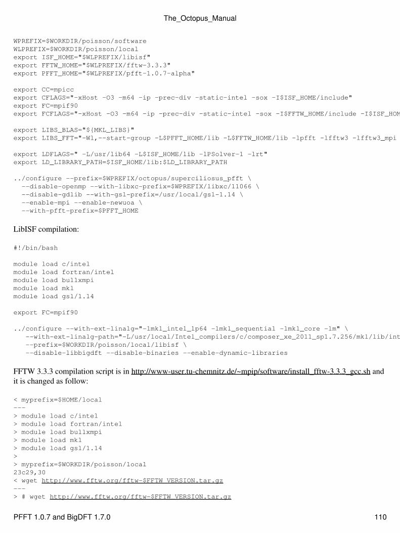
WPREFIX=$WORKDIR/poisson/softwareWLPREFIX=$WORKDIR/poisson/localexport ISF_HOME="$WLPREFIX/libisf"export FFTW_HOME="$WLPREFIX/fftw-3.3.3"export PFFT_HOME="$WLPREFIX/pfft-1.0.7-alpha"
export CC=mpiccexport CFLAGS="-xHost -O3 -m64 -ip -prec-div -static-intel -sox -I$ISF_HOME/include"export FC=mpif90export FCFLAGS="-xHost -O3 -m64 -ip -prec-div -static-intel -sox -I$FFTW_HOME/include -I$ISF_HOME/include"
export LIBS_BLAS="${MKL_LIBS}"export LIBS_FFT="-Wl,--start-group -L$PFFT_HOME/lib -L$FFTW_HOME/lib -lpfft -lfftw3 -lfftw3_mpi -Wl,--end-group"
export LDFLAGS=" -L/usr/lib64 -L$ISF_HOME/lib -lPSolver-1 -lrt"export LD_LIBRARY_PATH=$ISF_HOME/lib:$LD_LIBRARY_PATH
../configure --prefix=$WPREFIX/octopus/superciliosus_pfft \ --disable-openmp --with-libxc-prefix=$WPREFIX/libxc/11066 \ --disable-gdlib --with-gsl-prefix=/usr/local/gsl-1.14 \ --enable-mpi --enable-newuoa \ --with-pfft-prefix=$PFFT_HOME
LibISF compilation:
#!/bin/bash
module load c/intelmodule load fortran/intelmodule load bullxmpimodule load mklmodule load gsl/1.14
export FC=mpif90
../configure --with-ext-linalg="-lmkl_intel_lp64 -lmkl_sequential -lmkl_core -lm" \ --with-ext-linalg-path="-L/usr/local/Intel_compilers/c/composer_xe_2011_sp1.7.256/mkl/lib/intel64" \ --prefix=$WORKDIR/poisson/local/libisf \ --disable-libbigdft --disable-binaries --enable-dynamic-libraries
FFTW 3.3.3 compilation script is in http://www-user.tu-chemnitz.de/~mpip/software/install_fftw-3.3.3_gcc.sh andit is changed as follow:
< myprefix=$HOME/local--- > module load c/intel> module load fortran/intel> module load bullxmpi> module load mkl> module load gsl/1.14> > myprefix=$WORKDIR/poisson/local23c29,30< wget http://www.fftw.org/fftw-$FFTW_VERSION.tar.gz---> # wget http://www.fftw.org/fftw-$FFTW_VERSION.tar.gz
The_Octopus_Manual
PFFT 1.0.7 and BigDFT 1.7.0 110
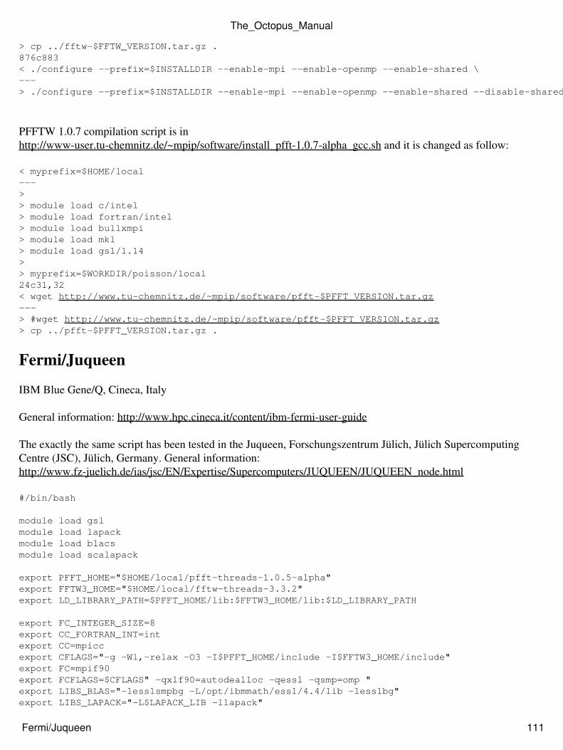
> cp ../fftw-$FFTW_VERSION.tar.gz .876c883< ./configure --prefix=$INSTALLDIR --enable-mpi --enable-openmp --enable-shared \---> ./configure --prefix=$INSTALLDIR --enable-mpi --enable-openmp --enable-shared --disable-shared \
PFFTW 1.0.7 compilation script is inhttp://www-user.tu-chemnitz.de/~mpip/software/install_pfft-1.0.7-alpha_gcc.sh and it is changed as follow:
< myprefix=$HOME/local---> > module load c/intel> module load fortran/intel> module load bullxmpi> module load mkl> module load gsl/1.14> > myprefix=$WORKDIR/poisson/local24c31,32< wget http://www.tu-chemnitz.de/~mpip/software/pfft-$PFFT_VERSION.tar.gz---> #wget http://www.tu-chemnitz.de/~mpip/software/pfft-$PFFT_VERSION.tar.gz> cp ../pfft-$PFFT_VERSION.tar.gz .
Fermi/Juqueen
IBM Blue Gene/Q, Cineca, Italy
General information: http://www.hpc.cineca.it/content/ibm-fermi-user-guide
The exactly the same script has been tested in the Juqueen, Forschungszentrum Jülich, Jülich SupercomputingCentre (JSC), Jülich, Germany. General information:http://www.fz-juelich.de/ias/jsc/EN/Expertise/Supercomputers/JUQUEEN/JUQUEEN_node.html
#/bin/bash
module load gslmodule load lapackmodule load blacsmodule load scalapack
export PFFT_HOME="$HOME/local/pfft-threads-1.0.5-alpha"export FFTW3_HOME="$HOME/local/fftw-threads-3.3.2"export LD_LIBRARY_PATH=$PFFT_HOME/lib:$FFTW3_HOME/lib:$LD_LIBRARY_PATH
export FC_INTEGER_SIZE=8export CC_FORTRAN_INT=intexport CC=mpiccexport CFLAGS="-g -Wl,-relax -O3 -I$PFFT_HOME/include -I$FFTW3_HOME/include"export FC=mpif90export FCFLAGS=$CFLAGS" -qxlf90=autodealloc -qessl -qsmp=omp "export LIBS_BLAS="-lesslsmpbg -L/opt/ibmmath/essl/4.4/lib -lesslbg"export LIBS_LAPACK="-L$LAPACK_LIB -llapack"
The_Octopus_Manual
Fermi/Juqueen 111
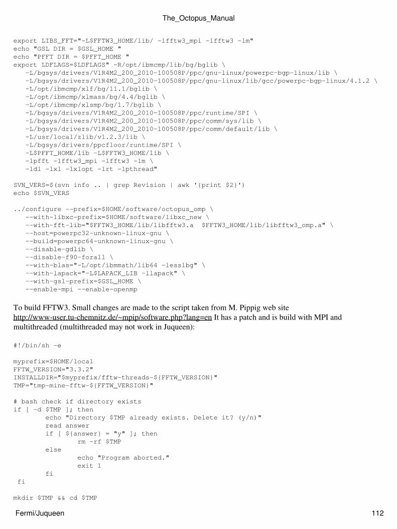
export LIBS_FFT="-L$FFTW3_HOME/lib/ -lfftw3_mpi -lfftw3 -lm"echo "GSL DIR = $GSL_HOME "echo "PFFT DIR = $PFFT_HOME "export LDFLAGS=$LDFLAGS" -R/opt/ibmcmp/lib/bg/bglib \ -L/bgsys/drivers/V1R4M2_200_2010-100508P/ppc/gnu-linux/powerpc-bgp-linux/lib \ -L/bgsys/drivers/V1R4M2_200_2010-100508P/ppc/gnu-linux/lib/gcc/powerpc-bgp-linux/4.1.2 \ -L/opt/ibmcmp/xlf/bg/11.1/bglib \ -L/opt/ibmcmp/xlmass/bg/4.4/bglib \ -L/opt/ibmcmp/xlsmp/bg/1.7/bglib \ -L/bgsys/drivers/V1R4M2_200_2010-100508P/ppc/runtime/SPI \ -L/bgsys/drivers/V1R4M2_200_2010-100508P/ppc/comm/sys/lib \ -L/bgsys/drivers/V1R4M2_200_2010-100508P/ppc/comm/default/lib \ -L/usr/local/zlib/v1.2.3/lib \ -L/bgsys/drivers/ppcfloor/runtime/SPI \ -L$PFFT_HOME/lib -L$FFTW3_HOME/lib \ -lpfft -lfftw3_mpi -lfftw3 -lm \ -ldl -lxl -lxlopt -lrt -lpthread"
SVN_VERS=$(svn info .. | grep Revision | awk '{print $2}')echo $SVN_VERS
../configure --prefix=$HOME/software/octopus_omp \ --with-libxc-prefix=$HOME/software/libxc_new \ --with-fft-lib="$FFTW3_HOME/lib/libfftw3.a $FFTW3_HOME/lib/libfftw3_omp.a" \ --host=powerpc32-unknown-linux-gnu \ --build=powerpc64-unknown-linux-gnu \ --disable-gdlib \ --disable-f90-forall \ --with-blas="-L/opt/ibmmath/lib64 -lesslbg" \ --with-lapack="-L$LAPACK_LIB -llapack" \ --with-gsl-prefix=$GSL_HOME \ --enable-mpi --enable-openmp
To build FFTW3. Small changes are made to the script taken from M. Pippig web sitehttp://www-user.tu-chemnitz.de/~mpip/software.php?lang=en It has a patch and is build with MPI andmultithreaded (multithreaded may not work in Juqueen):
#!/bin/sh -e
myprefix=$HOME/localFFTW_VERSION="3.3.2"INSTALLDIR="$myprefix/fftw-threads-${FFTW_VERSION}"TMP="tmp-mine-fftw-${FFTW_VERSION}"
# bash check if directory existsif [ -d $TMP ]; then echo "Directory $TMP already exists. Delete it? (y/n)" read answer if [ ${answer} = "y" ]; then rm -rf $TMP else echo "Program aborted." exit 1 fi fi
mkdir $TMP && cd $TMP
The_Octopus_Manual
Fermi/Juqueen 112
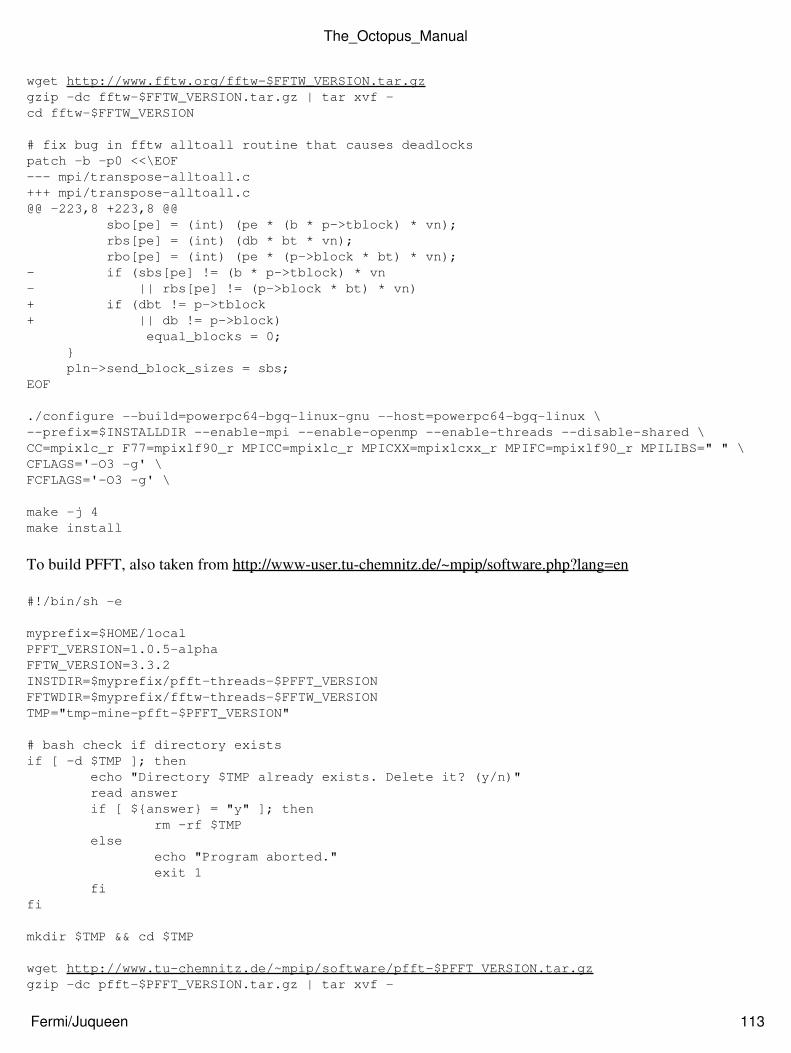
wget http://www.fftw.org/fftw-$FFTW_VERSION.tar.gzgzip -dc fftw-$FFTW_VERSION.tar.gz | tar xvf -cd fftw-$FFTW_VERSION
# fix bug in fftw alltoall routine that causes deadlockspatch -b -p0 <<\EOF--- mpi/transpose-alltoall.c+++ mpi/transpose-alltoall.c@@ -223,8 +223,8 @@ sbo[pe] = (int) (pe * (b * p->tblock) * vn); rbs[pe] = (int) (db * bt * vn); rbo[pe] = (int) (pe * (p->block * bt) * vn);- if (sbs[pe] != (b * p->tblock) * vn- || rbs[pe] != (p->block * bt) * vn)+ if (dbt != p->tblock+ || db != p->block) equal_blocks = 0; } pln->send_block_sizes = sbs;EOF
./configure --build=powerpc64-bgq-linux-gnu --host=powerpc64-bgq-linux \--prefix=$INSTALLDIR --enable-mpi --enable-openmp --enable-threads --disable-shared \CC=mpixlc_r F77=mpixlf90_r MPICC=mpixlc_r MPICXX=mpixlcxx_r MPIFC=mpixlf90_r MPILIBS=" " \CFLAGS='-O3 -g' \FCFLAGS='-O3 -g' \
make -j 4make install
To build PFFT, also taken from http://www-user.tu-chemnitz.de/~mpip/software.php?lang=en
#!/bin/sh -e
myprefix=$HOME/localPFFT_VERSION=1.0.5-alphaFFTW_VERSION=3.3.2INSTDIR=$myprefix/pfft-threads-$PFFT_VERSIONFFTWDIR=$myprefix/fftw-threads-$FFTW_VERSIONTMP="tmp-mine-pfft-$PFFT_VERSION"
# bash check if directory existsif [ -d $TMP ]; then echo "Directory $TMP already exists. Delete it? (y/n)" read answer if [ ${answer} = "y" ]; then rm -rf $TMP else echo "Program aborted." exit 1 fifi
mkdir $TMP && cd $TMP
wget http://www.tu-chemnitz.de/~mpip/software/pfft-$PFFT_VERSION.tar.gzgzip -dc pfft-$PFFT_VERSION.tar.gz | tar xvf -
The_Octopus_Manual
Fermi/Juqueen 113
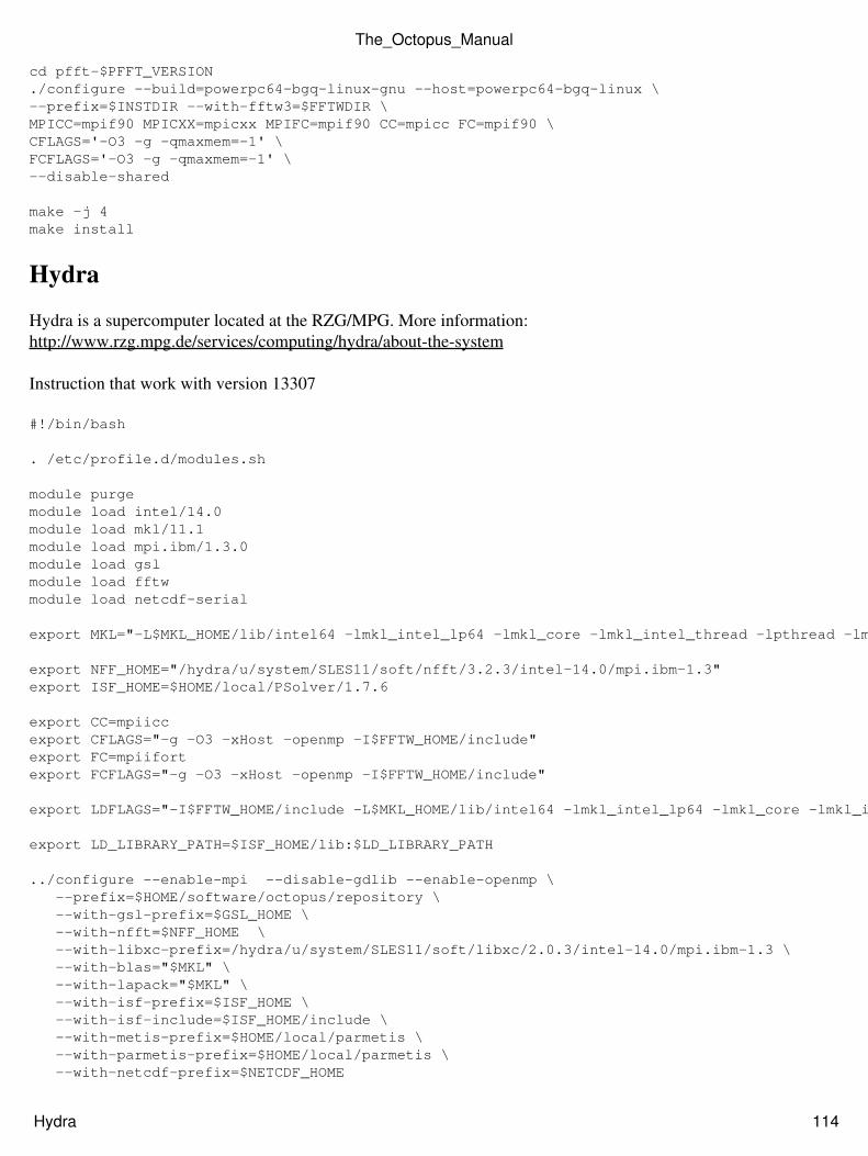
cd pfft-$PFFT_VERSION./configure --build=powerpc64-bgq-linux-gnu --host=powerpc64-bgq-linux \--prefix=$INSTDIR --with-fftw3=$FFTWDIR \MPICC=mpif90 MPICXX=mpicxx MPIFC=mpif90 CC=mpicc FC=mpif90 \CFLAGS='-O3 -g -qmaxmem=-1' \FCFLAGS='-O3 -g -qmaxmem=-1' \--disable-shared
make -j 4make install
Hydra
Hydra is a supercomputer located at the RZG/MPG. More information:http://www.rzg.mpg.de/services/computing/hydra/about-the-system
Instruction that work with version 13307
#!/bin/bash
. /etc/profile.d/modules.sh
module purge module load intel/14.0 module load mkl/11.1 module load mpi.ibm/1.3.0 module load gsl module load fftwmodule load netcdf-serial
export MKL="-L$MKL_HOME/lib/intel64 -lmkl_intel_lp64 -lmkl_core -lmkl_intel_thread -lpthread -lm"
export NFF_HOME="/hydra/u/system/SLES11/soft/nfft/3.2.3/intel-14.0/mpi.ibm-1.3"export ISF_HOME=$HOME/local/PSolver/1.7.6
export CC=mpiicc export CFLAGS="-g -O3 -xHost -openmp -I$FFTW_HOME/include"export FC=mpiifort export FCFLAGS="-g -O3 -xHost -openmp -I$FFTW_HOME/include"
export LDFLAGS="-I$FFTW_HOME/include -L$MKL_HOME/lib/intel64 -lmkl_intel_lp64 -lmkl_core -lmkl_intel_thread -lpthread -lm -Xlinker -rpath=$MKL_HOME/lib/intel64:$GSL_HOME/lib:$NETCDF_HOME/lib:$NFF_HOME/lib"
export LD_LIBRARY_PATH=$ISF_HOME/lib:$LD_LIBRARY_PATH
../configure --enable-mpi --disable-gdlib --enable-openmp \ --prefix=$HOME/software/octopus/repository \ --with-gsl-prefix=$GSL_HOME \ --with-nfft=$NFF_HOME \ --with-libxc-prefix=/hydra/u/system/SLES11/soft/libxc/2.0.3/intel-14.0/mpi.ibm-1.3 \ --with-blas="$MKL" \ --with-lapack="$MKL" \ --with-isf-prefix=$ISF_HOME \ --with-isf-include=$ISF_HOME/include \ --with-metis-prefix=$HOME/local/parmetis \ --with-parmetis-prefix=$HOME/local/parmetis \ --with-netcdf-prefix=$NETCDF_HOME
The_Octopus_Manual
Hydra 114
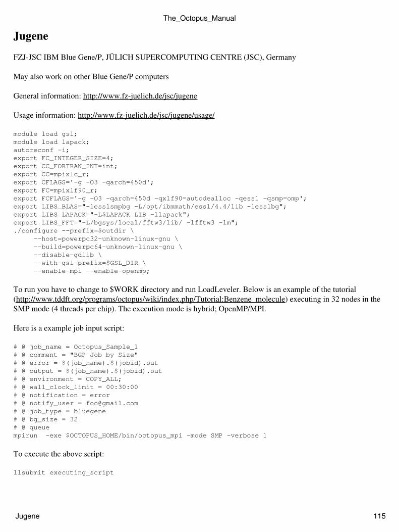
Jugene
FZJ-JSC IBM Blue Gene/P, JÜLICH SUPERCOMPUTING CENTRE (JSC), Germany
May also work on other Blue Gene/P computers
General information: http://www.fz-juelich.de/jsc/jugene
Usage information: http://www.fz-juelich.de/jsc/jugene/usage/
module load gsl;module load lapack;autoreconf -i;export FC_INTEGER_SIZE=4;export CC_FORTRAN_INT=int;export CC=mpixlc_r;export CFLAGS='-g -O3 -qarch=450d';export FC=mpixlf90_r;export FCFLAGS='-g -O3 -qarch=450d -qxlf90=autodealloc -qessl -qsmp=omp';export LIBS_BLAS="-lesslsmpbg -L/opt/ibmmath/essl/4.4/lib -lesslbg";export LIBS_LAPACK="-L$LAPACK_LIB -llapack";export LIBS_FFT="-L/bgsys/local/fftw3/lib/ -lfftw3 -lm";./configure --prefix=$outdir \ --host=powerpc32-unknown-linux-gnu \ --build=powerpc64-unknown-linux-gnu \ --disable-gdlib \ --with-gsl-prefix=$GSL_DIR \ --enable-mpi --enable-openmp;
To run you have to change to $WORK directory and run LoadLeveler. Below is an example of the tutorial(http://www.tddft.org/programs/octopus/wiki/index.php/Tutorial:Benzene_molecule) executing in 32 nodes in theSMP mode (4 threads per chip). The execution mode is hybrid; OpenMP/MPI.
Here is a example job input script:
# @ job_name = Octopus_Sample_1# @ comment = "BGP Job by Size"# @ error = $(job_name).$(jobid).out# @ output = $(job_name).$(jobid).out# @ environment = COPY_ALL;# @ wall_clock_limit = 00:30:00# @ notification = error# @ notify_user = [email protected]# @ job_type = bluegene# @ bg_size = 32# @ queuempirun -exe $OCTOPUS_HOME/bin/octopus_mpi -mode SMP -verbose 1
To execute the above script:
llsubmit executing_script
The_Octopus_Manual
Jugene 115
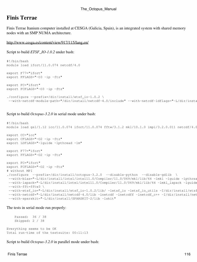
Finis Terrae
Finis Terrae Itanium computer installed at CESGA (Galicia, Spain), is an integrated system with shared memorynodes with an SMP NUMA architecture.
http://www.cesga.es/content/view/917/115/lang,en/
Script to build ETSF_IO-1.0.2 under bash:
#!/bin/bashmodule load ifort/11.0.074 netcdf/4.0
export F77="ifort"export FFLAGS="-O3 -ip -ftz"
export FC="ifort"export FCFLAGS="-O3 -ip -ftz"
./configure --prefix=/dir/install/etsf_io-1.0.2 \ --with-netcdf-module-path="/dir/install/netcdf-4.0/include" --with-netcdf-ldflags="-L/dir/install/netcdf-4.0/lib -lnetcdf -lnetcdff -lnetcdf_c++"
Script to build Octopus-3.2.0 in serial mode under bash:
#!/bin/bashmodule load gsl/1.12 icc/11.0.074 ifort/11.0.074 fftw/3.1.2 mkl/10.1.0 impi/3.2.0.011 netcdf/4.0 sparskit/2 etsf_io/1.0.2
export CC="icc"export CFLAGS="-O2 -ip -ftz" export LDFLAGS="-lguide -lpthread -lm"
export F77="ifort"export FFLAGS="-O2 -ip -ftz"
export FC="ifort"export FCFLAGS="-O2 -ip -ftz" # without MPI./configure --prefix=/dir/install/octopus-3.2.0 --disable-python --disable-gdlib \ --with-blas="-L/dir/install/intel/intel11.0/Compiler/11.0/069/mkl/lib/64 -lmkl -lguide -lpthread" \ --with-lapack="-L/dir/install/intel/intel11.0/Compiler/11.0/069/mkl/lib/64 -lmkl_lapack -lguide -lpthread" \ --with-fft=fftw3 \ --with-etsf_io="-L/dir/install/etsf_io-1.0.2/lib/ -letsf_io -letsf_io_utils -I/dir/install/etsf_io-1.0.2/include/intel/" \ --with-netcdf="-L/dir/install/netcdf-4.0/lib -lnetcdf -lnetcdff -lnetcdf_c++ -I/dir/install/netcdf-4.0/include" \ --with-sparskit="-L/dir/install/SPARSKIT-2/lib -lskit"
The tests in serial mode run properly:
Passed: 36 / 38 Skipped: 2 / 38
Everything seems to be OKTotal run-time of the testsuite: 00:11:13
Script to build Octopus-3.2.0 in parallel mode under bash:
The_Octopus_Manual
Finis Terrae 116
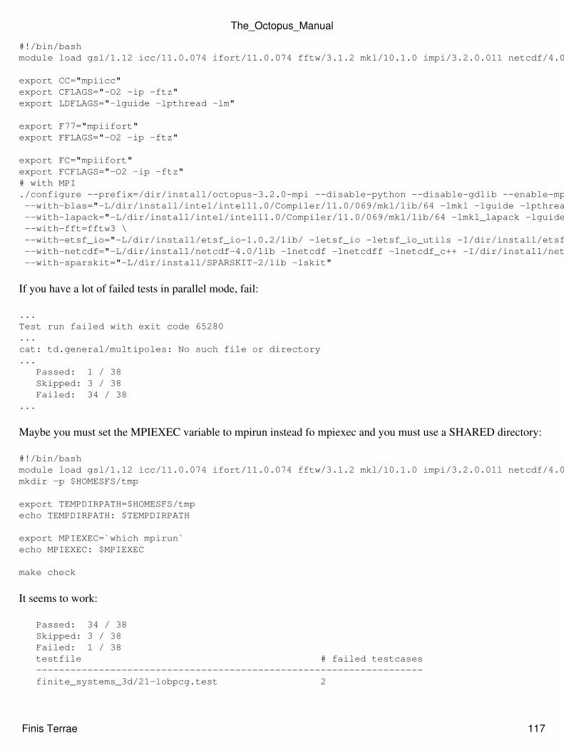
#!/bin/bashmodule load gsl/1.12 icc/11.0.074 ifort/11.0.074 fftw/3.1.2 mkl/10.1.0 impi/3.2.0.011 netcdf/4.0 sparskit/2 etsf_io/1.0.2
export CC="mpiicc"export CFLAGS="-O2 -ip -ftz"export LDFLAGS="-lguide -lpthread -lm"
export F77="mpiifort"export FFLAGS="-O2 -ip -ftz"
export FC="mpiifort"export FCFLAGS="-O2 -ip -ftz"# with MPI./configure --prefix=/dir/install/octopus-3.2.0-mpi --disable-python --disable-gdlib --enable-mpi \ --with-blas="-L/dir/install/intel/intel11.0/Compiler/11.0/069/mkl/lib/64 -lmkl -lguide -lpthread" \ --with-lapack="-L/dir/install/intel/intel11.0/Compiler/11.0/069/mkl/lib/64 -lmkl_lapack -lguide -lpthread" \ --with-fft=fftw3 \ --with-etsf_io="-L/dir/install/etsf_io-1.0.2/lib/ -letsf_io -letsf_io_utils -I/dir/install/etsf_io-1.0.2/include/intel/" \ --with-netcdf="-L/dir/install/netcdf-4.0/lib -lnetcdf -lnetcdff -lnetcdf_c++ -I/dir/install/netcdf-4.0/include" \ --with-sparskit="-L/dir/install/SPARSKIT-2/lib -lskit"
If you have a lot of failed tests in parallel mode, fail:
...Test run failed with exit code 65280...cat: td.general/multipoles: No such file or directory... Passed: 1 / 38 Skipped: 3 / 38 Failed: 34 / 38...
Maybe you must set the MPIEXEC variable to mpirun instead fo mpiexec and you must use a SHARED directory:
#!/bin/bashmodule load gsl/1.12 icc/11.0.074 ifort/11.0.074 fftw/3.1.2 mkl/10.1.0 impi/3.2.0.011 netcdf/4.0 sparskit/2 etsf_io/1.0.2mkdir -p $HOMESFS/tmp
export TEMPDIRPATH=$HOMESFS/tmpecho TEMPDIRPATH: $TEMPDIRPATH
export MPIEXEC=`which mpirun`echo MPIEXEC: $MPIEXEC
make check
It seems to work:
Passed: 34 / 38 Skipped: 3 / 38 Failed: 1 / 38 testfile # failed testcases -------------------------------------------------------------------- finite_systems_3d/21-lobpcg.test 2
The_Octopus_Manual
Finis Terrae 117
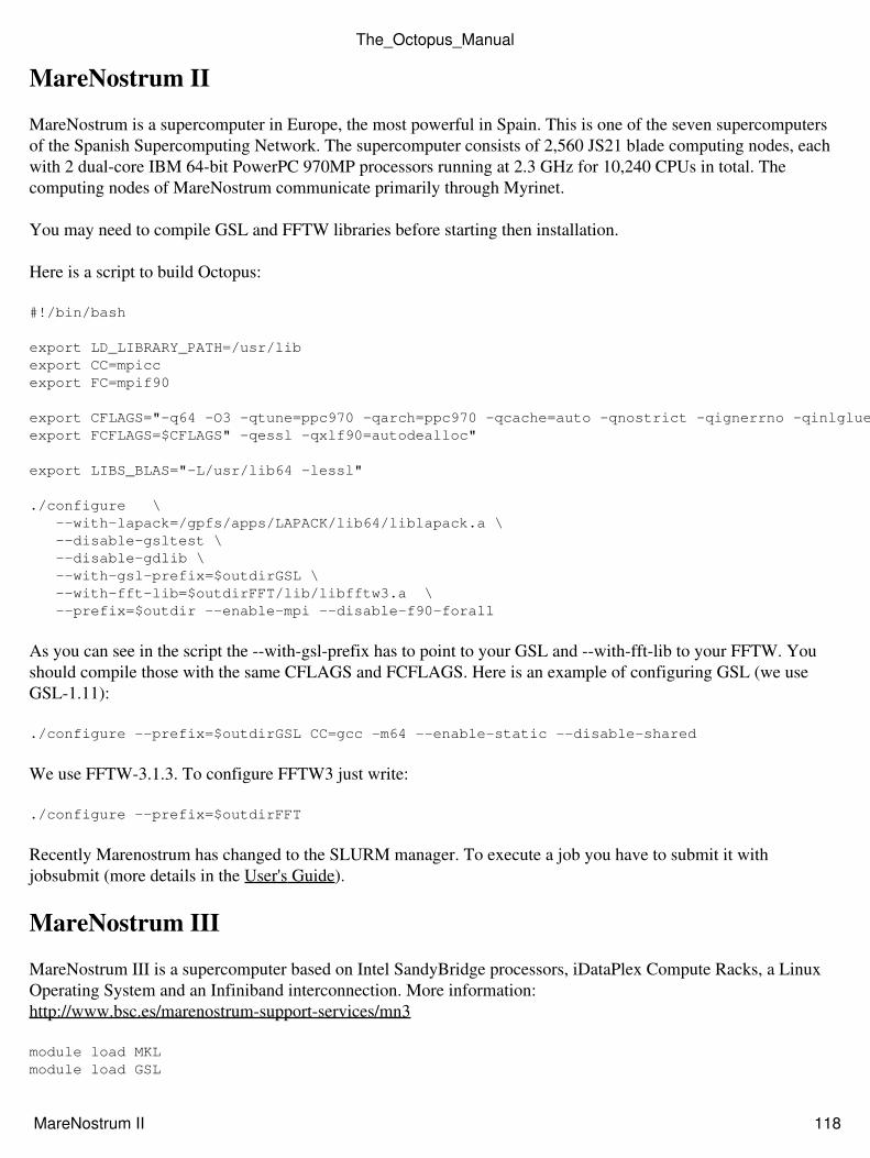
MareNostrum II
MareNostrum is a supercomputer in Europe, the most powerful in Spain. This is one of the seven supercomputersof the Spanish Supercomputing Network. The supercomputer consists of 2,560 JS21 blade computing nodes, eachwith 2 dual-core IBM 64-bit PowerPC 970MP processors running at 2.3 GHz for 10,240 CPUs in total. Thecomputing nodes of MareNostrum communicate primarily through Myrinet.
You may need to compile GSL and FFTW libraries before starting then installation.
Here is a script to build Octopus:
#!/bin/bash
export LD_LIBRARY_PATH=/usr/libexport CC=mpiccexport FC=mpif90
export CFLAGS="-q64 -O3 -qtune=ppc970 -qarch=ppc970 -qcache=auto -qnostrict -qignerrno -qinlglue"export FCFLAGS=$CFLAGS" -qessl -qxlf90=autodealloc"
export LIBS_BLAS="-L/usr/lib64 -lessl"
./configure \ --with-lapack=/gpfs/apps/LAPACK/lib64/liblapack.a \ --disable-gsltest \ --disable-gdlib \ --with-gsl-prefix=$outdirGSL \ --with-fft-lib=$outdirFFT/lib/libfftw3.a \ --prefix=$outdir --enable-mpi --disable-f90-forall
As you can see in the script the --with-gsl-prefix has to point to your GSL and --with-fft-lib to your FFTW. Youshould compile those with the same CFLAGS and FCFLAGS. Here is an example of configuring GSL (we useGSL-1.11):
./configure --prefix=$outdirGSL CC=gcc -m64 --enable-static --disable-shared
We use FFTW-3.1.3. To configure FFTW3 just write:
./configure --prefix=$outdirFFT
Recently Marenostrum has changed to the SLURM manager. To execute a job you have to submit it withjobsubmit (more details in the User's Guide).
MareNostrum III
MareNostrum III is a supercomputer based on Intel SandyBridge processors, iDataPlex Compute Racks, a LinuxOperating System and an Infiniband interconnection. More information:http://www.bsc.es/marenostrum-support-services/mn3
module load MKLmodule load GSL
The_Octopus_Manual
MareNostrum II 118
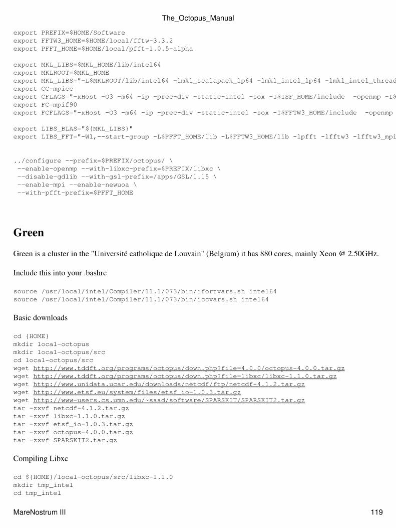
export PREFIX=$HOME/Softwareexport FFTW3_HOME=$HOME/local/fftw-3.3.2export PFFT_HOME=$HOME/local/pfft-1.0.5-alpha
export MKL_LIBS=$MKL_HOME/lib/intel64export MKLROOT=$MKL_HOMEexport MKL_LIBS="-L$MKLROOT/lib/intel64 -lmkl_scalapack_lp64 -lmkl_intel_lp64 -lmkl_intel_thread -lmkl_core -lmkl_blacs_intelmpi_lp64 -lpthread -lm"export CC=mpiccexport CFLAGS="-xHost -O3 -m64 -ip -prec-div -static-intel -sox -I$ISF_HOME/include -openmp -I$MKLROOT/include"export FC=mpif90export FCFLAGS="-xHost -O3 -m64 -ip -prec-div -static-intel -sox -I$FFTW3_HOME/include -openmp -I$ISF_HOME/include -I$MKLROOT/include"
export LIBS_BLAS="${MKL_LIBS}"export LIBS_FFT="-Wl,--start-group -L$PFFT_HOME/lib -L$FFTW3_HOME/lib -lpfft -lfftw3 -lfftw3_mpi -Wl,--end-group"
../configure --prefix=$PREFIX/octopus/ \ --enable-openmp --with-libxc-prefix=$PREFIX/libxc \ --disable-gdlib --with-gsl-prefix=/apps/GSL/1.15 \ --enable-mpi --enable-newuoa \ --with-pfft-prefix=$PFFT_HOME
Green
Green is a cluster in the "Université catholique de Louvain" (Belgium) it has 880 cores, mainly Xeon @ 2.50GHz.
Include this into your .bashrc
source /usr/local/intel/Compiler/11.1/073/bin/ifortvars.sh intel64source /usr/local/intel/Compiler/11.1/073/bin/iccvars.sh intel64
Basic downloads
cd {HOME}mkdir local-octopusmkdir local-octopus/srccd local-octopus/srcwget http://www.tddft.org/programs/octopus/down.php?file=4.0.0/octopus-4.0.0.tar.gzwget http://www.tddft.org/programs/octopus/down.php?file=libxc/libxc-1.1.0.tar.gzwget http://www.unidata.ucar.edu/downloads/netcdf/ftp/netcdf-4.1.2.tar.gzwget http://www.etsf.eu/system/files/etsf_io-1.0.3.tar.gzwget http://www-users.cs.umn.edu/~saad/software/SPARSKIT/SPARSKIT2.tar.gztar -zxvf netcdf-4.1.2.tar.gztar -zxvf libxc-1.1.0.tar.gz tar -zxvf etsf_io-1.0.3.tar.gztar -zxvf octopus-4.0.0.tar.gztar -zxvf SPARSKIT2.tar.gz
Compiling Libxc
cd ${HOME}/local-octopus/src/libxc-1.1.0mkdir tmp_intelcd tmp_intel
The_Octopus_Manual
MareNostrum III 119
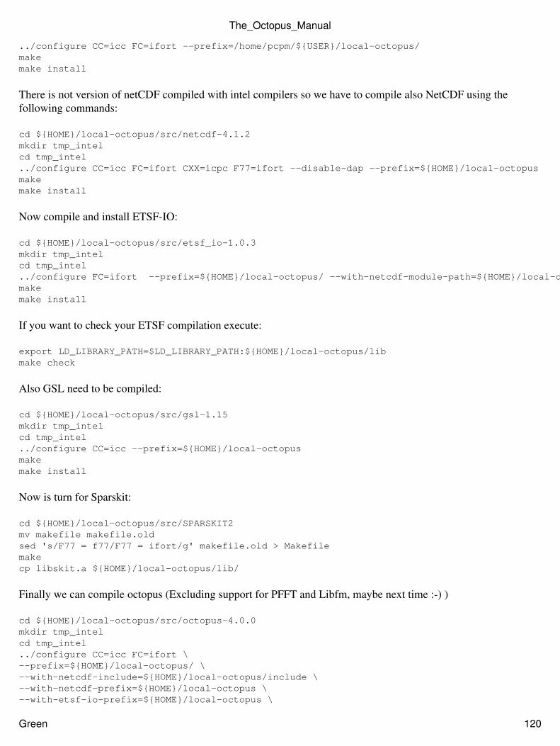
../configure CC=icc FC=ifort --prefix=/home/pcpm/${USER}/local-octopus/makemake install
There is not version of netCDF compiled with intel compilers so we have to compile also NetCDF using thefollowing commands:
cd ${HOME}/local-octopus/src/netcdf-4.1.2mkdir tmp_intelcd tmp_intel../configure CC=icc FC=ifort CXX=icpc F77=ifort --disable-dap --prefix=${HOME}/local-octopusmakemake install
Now compile and install ETSF-IO:
cd ${HOME}/local-octopus/src/etsf_io-1.0.3mkdir tmp_intelcd tmp_intel../configure FC=ifort --prefix=${HOME}/local-octopus/ --with-netcdf-module-path=${HOME}/local-octopus/include --with-netcdf-ldflags=-L${HOME}/local-octopus/libmakemake install
If you want to check your ETSF compilation execute:
export LD_LIBRARY_PATH=$LD_LIBRARY_PATH:${HOME}/local-octopus/libmake check
Also GSL need to be compiled:
cd ${HOME}/local-octopus/src/gsl-1.15mkdir tmp_intelcd tmp_intel../configure CC=icc --prefix=${HOME}/local-octopusmakemake install
Now is turn for Sparskit:
cd ${HOME}/local-octopus/src/SPARSKIT2mv makefile makefile.oldsed 's/F77 = f77/F77 = ifort/g' makefile.old > Makefilemakecp libskit.a ${HOME}/local-octopus/lib/
Finally we can compile octopus (Excluding support for PFFT and Libfm, maybe next time :-) )
cd ${HOME}/local-octopus/src/octopus-4.0.0mkdir tmp_intelcd tmp_intel../configure CC=icc FC=ifort \--prefix=${HOME}/local-octopus/ \--with-netcdf-include=${HOME}/local-octopus/include \--with-netcdf-prefix=${HOME}/local-octopus \--with-etsf-io-prefix=${HOME}/local-octopus \
The_Octopus_Manual
Green 120
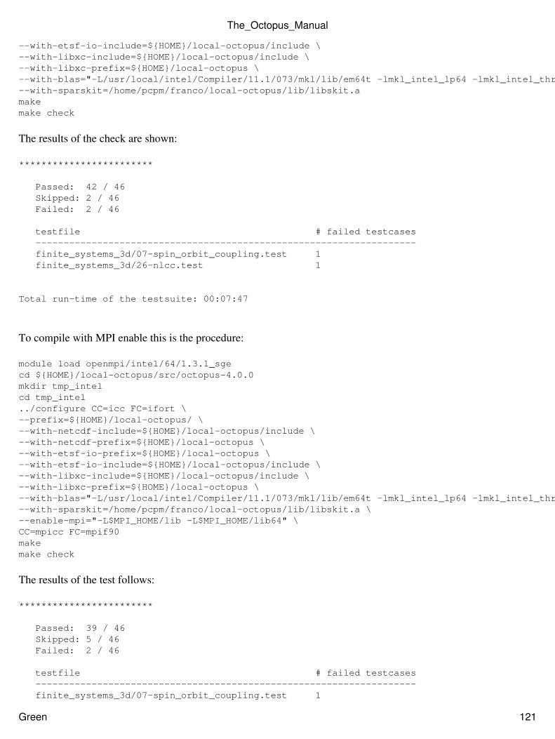
--with-etsf-io-include=${HOME}/local-octopus/include \--with-libxc-include=${HOME}/local-octopus/include \--with-libxc-prefix=${HOME}/local-octopus \--with-blas="-L/usr/local/intel/Compiler/11.1/073/mkl/lib/em64t -lmkl_intel_lp64 -lmkl_intel_thread -lmkl_core -liomp5 -lpthread" \--with-sparskit=/home/pcpm/franco/local-octopus/lib/libskit.amakemake check
The results of the check are shown:
************************
Passed: 42 / 46 Skipped: 2 / 46 Failed: 2 / 46
testfile # failed testcases -------------------------------------------------------------------- finite_systems_3d/07-spin_orbit_coupling.test 1 finite_systems_3d/26-nlcc.test 1
Total run-time of the testsuite: 00:07:47
To compile with MPI enable this is the procedure:
module load openmpi/intel/64/1.3.1_sgecd ${HOME}/local-octopus/src/octopus-4.0.0mkdir tmp_intelcd tmp_intel../configure CC=icc FC=ifort \--prefix=${HOME}/local-octopus/ \--with-netcdf-include=${HOME}/local-octopus/include \--with-netcdf-prefix=${HOME}/local-octopus \--with-etsf-io-prefix=${HOME}/local-octopus \--with-etsf-io-include=${HOME}/local-octopus/include \--with-libxc-include=${HOME}/local-octopus/include \--with-libxc-prefix=${HOME}/local-octopus \--with-blas="-L/usr/local/intel/Compiler/11.1/073/mkl/lib/em64t -lmkl_intel_lp64 -lmkl_intel_thread -lmkl_core -liomp5 -lpthread" \--with-sparskit=/home/pcpm/franco/local-octopus/lib/libskit.a \--enable-mpi="-L$MPI_HOME/lib -L$MPI_HOME/lib64" \CC=mpicc FC=mpif90makemake check
The results of the test follows:
************************
Passed: 39 / 46 Skipped: 5 / 46 Failed: 2 / 46
testfile # failed testcases -------------------------------------------------------------------- finite_systems_3d/07-spin_orbit_coupling.test 1
The_Octopus_Manual
Green 121
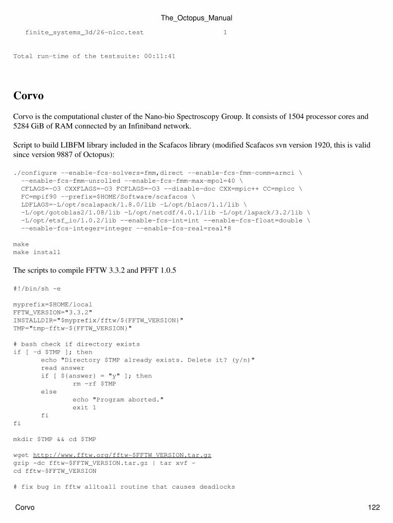
finite_systems_3d/26-nlcc.test 1
Total run-time of the testsuite: 00:11:41
Corvo
Corvo is the computational cluster of the Nano-bio Spectroscopy Group. It consists of 1504 processor cores and5284 GiB of RAM connected by an Infiniband network.
Script to build LIBFM library included in the Scafacos library (modified Scafacos svn version 1920, this is validsince version 9887 of Octopus):
./configure --enable-fcs-solvers=fmm,direct --enable-fcs-fmm-comm=armci \ --enable-fcs-fmm-unrolled --enable-fcs-fmm-max-mpol=40 \ CFLAGS=-O3 CXXFLAGS=-O3 FCFLAGS=-O3 --disable-doc CXX=mpic++ CC=mpicc \ FC=mpif90 --prefix=$HOME/Software/scafacos \ LDFLAGS=-L/opt/scalapack/1.8.0/lib -L/opt/blacs/1.1/lib \ -L/opt/gotoblas2/1.08/lib -L/opt/netcdf/4.0.1/lib -L/opt/lapack/3.2/lib \ -L/opt/etsf_io/1.0.2/lib --enable-fcs-int=int --enable-fcs-float=double \ --enable-fcs-integer=integer --enable-fcs-real=real*8
makemake install
The scripts to compile FFTW 3.3.2 and PFFT 1.0.5
#!/bin/sh -e
myprefix=$HOME/localFFTW_VERSION="3.3.2"INSTALLDIR="$myprefix/fftw/${FFTW_VERSION}"TMP="tmp-fftw-${FFTW_VERSION}"
# bash check if directory existsif [ -d $TMP ]; then echo "Directory $TMP already exists. Delete it? (y/n)" read answer if [ ${answer} = "y" ]; then rm -rf $TMP else echo "Program aborted." exit 1 fifi
mkdir $TMP && cd $TMP
wget http://www.fftw.org/fftw-$FFTW_VERSION.tar.gzgzip -dc fftw-$FFTW_VERSION.tar.gz | tar xvf -cd fftw-$FFTW_VERSION
# fix bug in fftw alltoall routine that causes deadlocks
The_Octopus_Manual
Corvo 122
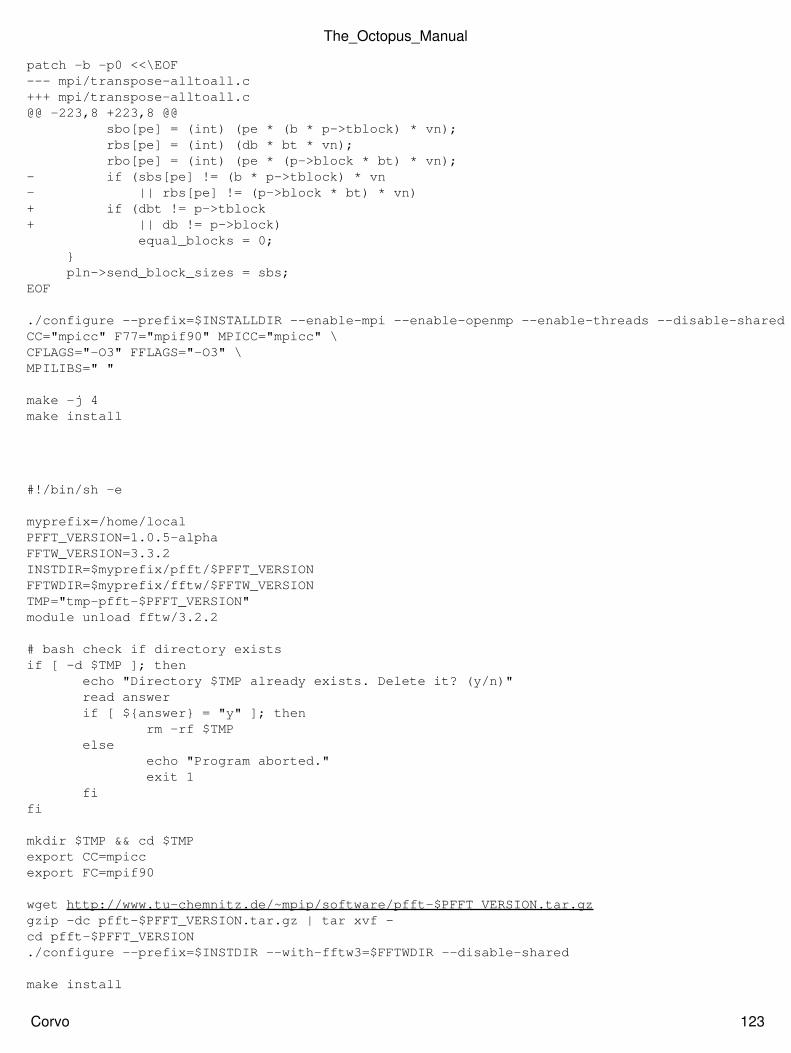
patch -b -p0 <<\EOF--- mpi/transpose-alltoall.c+++ mpi/transpose-alltoall.c@@ -223,8 +223,8 @@ sbo[pe] = (int) (pe * (b * p->tblock) * vn); rbs[pe] = (int) (db * bt * vn); rbo[pe] = (int) (pe * (p->block * bt) * vn);- if (sbs[pe] != (b * p->tblock) * vn- || rbs[pe] != (p->block * bt) * vn)+ if (dbt != p->tblock+ || db != p->block) equal_blocks = 0; } pln->send_block_sizes = sbs;EOF
./configure --prefix=$INSTALLDIR --enable-mpi --enable-openmp --enable-threads --disable-shared \CC="mpicc" F77="mpif90" MPICC="mpicc" \CFLAGS="-O3" FFLAGS="-O3" \MPILIBS=" "
make -j 4make install
#!/bin/sh -e
myprefix=/home/localPFFT_VERSION=1.0.5-alphaFFTW_VERSION=3.3.2INSTDIR=$myprefix/pfft/$PFFT_VERSIONFFTWDIR=$myprefix/fftw/$FFTW_VERSIONTMP="tmp-pfft-$PFFT_VERSION"module unload fftw/3.2.2
# bash check if directory existsif [ -d $TMP ]; then echo "Directory $TMP already exists. Delete it? (y/n)" read answer if [ ${answer} = "y" ]; then rm -rf $TMP else echo "Program aborted." exit 1 fifi
mkdir $TMP && cd $TMPexport CC=mpiccexport FC=mpif90
wget http://www.tu-chemnitz.de/~mpip/software/pfft-$PFFT_VERSION.tar.gzgzip -dc pfft-$PFFT_VERSION.tar.gz | tar xvf -cd pfft-$PFFT_VERSION./configure --prefix=$INSTDIR --with-fftw3=$FFTWDIR --disable-shared
make install
The_Octopus_Manual
Corvo 123
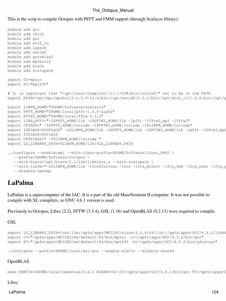
This is the scrip to compile Octopus with PFFT and FMM support (through Scafacos library):
module add gccmodule add ifortmodule add gslmodule add etsf_iomodule add lapackmodule add netcdfmodule add gotoblas2module add mpibull2 module add blacsmodule add scalapack
export CC=mpiccexport FC="mpif90"
# It is important that "/opt/intel/Compiler//11.1/038/bin/intel64/" not to be in the PATHexport PATH=/opt/mpi/mpibull2-1.3.9-14.s/bin:/opt/netcdf/4.0.1/bin:/opt/etsf_io/1.0.2/bin:/opt/gsl//1.13/bin:/opt/intel/composer_xe_2011_sp1.10.319//bin/intel64/:/opt/gcc//4.4/bin:/opt/slurm/bin:/usr/kerberos/bin:/opt/cuda//bin:/usr/local/bin:/bin:/usr/bin
export LIBFM_HOME="$HOME/Software/scafacos"export PFFT_HOME="$HOME/local/pfft-1.0.5-alpha"export FFTW3_HOME="$HOME/local/fftw-3.3.2"export LIBS_PFFT="-L$PFFT_HOME/lib -L$FFTW3_HOME/lib -lpfft -lfftw3_mpi -lfftw3"export CFLAGS=" -I$PFFT_HOME/include -I$FFTW3_HOME/include -I$LIBFM_HOME/include"export LDFLAGS=$LDFLAGS" -L$LIBFM_HOME/lib -L$PFFT_HOME/lib -L$FFTW3_HOME/lib -lpfft -lfftw3_mpi -lfftw3 -lm "export FCFLAGS=$CFLAGSexport CPPFLAGS=" -I$LIBFM_HOME/include "export LD_LIBRARY_PATH=$LIBFM_HOME/lib:$LD_LIBRARY_PATH
../configure --enable-mpi --with-libxc-prefix=$HOME/Software/libxc_9882 \ --prefix=$HOME/Software/octopus \ --with-blacs=/opt/blacs/1.1/lib/libblacs.a --with-scalapack \ --with-libfm="-L$LIBFM_HOME/lib -lfcs4fortran -lfcs -lfcs_direct -lfcs_fmm -lfcs_near -lfcs_gridsort -lfcs_common" \ --disable-openmp
LaPalma
LaPalma is a supercomputer of the IAC. It is a part of the old MareNostrum II computer. It was not possible tocompile with XL compilers, so GNU 4.6.1 version is used.
Previously to Octopus, Libxc (2.2), FFTW (3.3.4), GSL (1.16) and OpenBLAS (0.2.13) were required to compile.
GSL
export LD_LIBRARY_PATH=/usr/lib:/gpfs/apps/MPICH2/slurm-2.5.6/64/lib/:/gpfs/apps/GCC/4.9.2/lib64/export CC="/gpfs/apps/MPICH2/mx/default/64/bin/mpicc -cc=/gpfs/apps/GCC/4.9.2/bin/gcc"export FC="/gpfs/apps/MPICH2/mx/default/64/bin/mpif90 -fc=/gpfs/apps/GCC/4.9.2/bin/gfortran"
./configure --prefix=$HOME/local/gsl/gnu --enable-static --disable-shared
OpenBLAS
make PREFIX=$HOME/local/openblas/4.6.1 BINARY=64 CC=/gpfs/apps/GCC/4.6.1/bin/gcc FC=/gpfs/apps/GCC/4.6.1/bin/gfortran
Libxc
The_Octopus_Manual
LaPalma 124
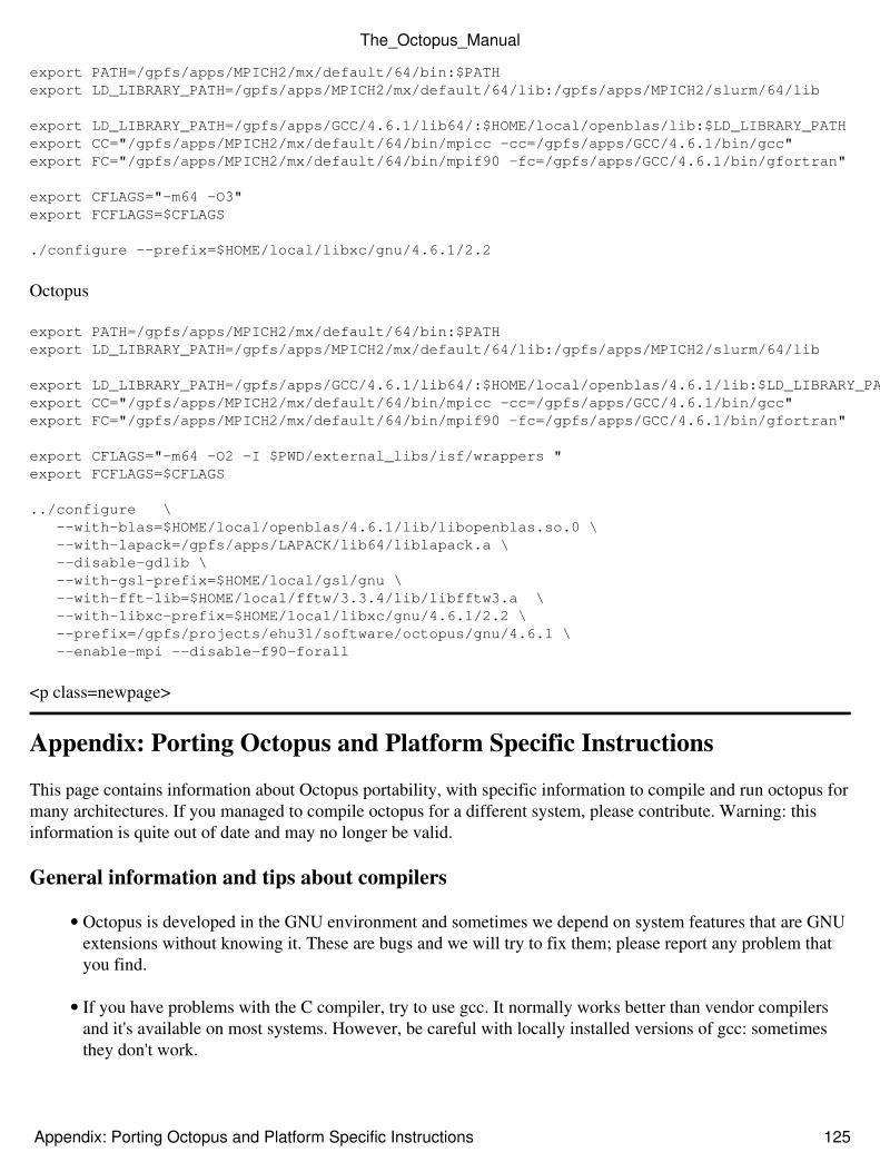
export PATH=/gpfs/apps/MPICH2/mx/default/64/bin:$PATHexport LD_LIBRARY_PATH=/gpfs/apps/MPICH2/mx/default/64/lib:/gpfs/apps/MPICH2/slurm/64/lib
export LD_LIBRARY_PATH=/gpfs/apps/GCC/4.6.1/lib64/:$HOME/local/openblas/lib:$LD_LIBRARY_PATHexport CC="/gpfs/apps/MPICH2/mx/default/64/bin/mpicc -cc=/gpfs/apps/GCC/4.6.1/bin/gcc"export FC="/gpfs/apps/MPICH2/mx/default/64/bin/mpif90 -fc=/gpfs/apps/GCC/4.6.1/bin/gfortran"
export CFLAGS="-m64 -O3"export FCFLAGS=$CFLAGS
./configure --prefix=$HOME/local/libxc/gnu/4.6.1/2.2
Octopus
export PATH=/gpfs/apps/MPICH2/mx/default/64/bin:$PATHexport LD_LIBRARY_PATH=/gpfs/apps/MPICH2/mx/default/64/lib:/gpfs/apps/MPICH2/slurm/64/lib
export LD_LIBRARY_PATH=/gpfs/apps/GCC/4.6.1/lib64/:$HOME/local/openblas/4.6.1/lib:$LD_LIBRARY_PATHexport CC="/gpfs/apps/MPICH2/mx/default/64/bin/mpicc -cc=/gpfs/apps/GCC/4.6.1/bin/gcc"export FC="/gpfs/apps/MPICH2/mx/default/64/bin/mpif90 -fc=/gpfs/apps/GCC/4.6.1/bin/gfortran"
export CFLAGS="-m64 -O2 -I $PWD/external_libs/isf/wrappers "export FCFLAGS=$CFLAGS
../configure \ --with-blas=$HOME/local/openblas/4.6.1/lib/libopenblas.so.0 \ --with-lapack=/gpfs/apps/LAPACK/lib64/liblapack.a \ --disable-gdlib \ --with-gsl-prefix=$HOME/local/gsl/gnu \ --with-fft-lib=$HOME/local/fftw/3.3.4/lib/libfftw3.a \ --with-libxc-prefix=$HOME/local/libxc/gnu/4.6.1/2.2 \ --prefix=/gpfs/projects/ehu31/software/octopus/gnu/4.6.1 \ --enable-mpi --disable-f90-forall
<p class=newpage>
Appendix: Porting Octopus and Platform Specific Instructions
This page contains information about Octopus portability, with specific information to compile and run octopus formany architectures. If you managed to compile octopus for a different system, please contribute. Warning: thisinformation is quite out of date and may no longer be valid.
General information and tips about compilers
Octopus is developed in the GNU environment and sometimes we depend on system features that are GNUextensions without knowing it. These are bugs and we will try to fix them; please report any problem thatyou find.
•
If you have problems with the C compiler, try to use gcc. It normally works better than vendor compilersand it's available on most systems. However, be careful with locally installed versions of gcc: sometimesthey don't work.
•
The_Octopus_Manual
Appendix: Porting Octopus and Platform Specific Instructions 125
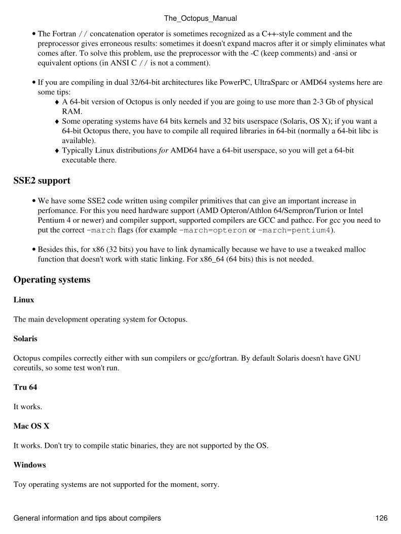
The Fortran // concatenation operator is sometimes recognized as a C++-style comment and thepreprocessor gives erroneous results: sometimes it doesn't expand macros after it or simply eliminates whatcomes after. To solve this problem, use the preprocessor with the -C (keep comments) and -ansi orequivalent options (in ANSI C // is not a comment).
•
If you are compiling in dual 32/64-bit architectures like PowerPC, UltraSparc or AMD64 systems here aresome tips:
A 64-bit version of Octopus is only needed if you are going to use more than 2-3 Gb of physicalRAM.
♦
Some operating systems have 64 bits kernels and 32 bits userspace (Solaris, OS X); if you want a64-bit Octopus there, you have to compile all required libraries in 64-bit (normally a 64-bit libc isavailable).
♦
Typically Linux distributions for AMD64 have a 64-bit userspace, so you will get a 64-bitexecutable there.
♦
•
SSE2 support
We have some SSE2 code written using compiler primitives that can give an important increase inperfomance. For this you need hardware support (AMD Opteron/Athlon 64/Sempron/Turion or IntelPentium 4 or newer) and compiler support, supported compilers are GCC and pathcc. For gcc you need toput the correct -march flags (for example -march=opteron or -march=pentium4).
•
Besides this, for x86 (32 bits) you have to link dynamically because we have to use a tweaked mallocfunction that doesn't work with static linking. For x86_64 (64 bits) this is not needed.
•
Operating systems
Linux
The main development operating system for Octopus.
Solaris
Octopus compiles correctly either with sun compilers or gcc/gfortran. By default Solaris doesn't have GNUcoreutils, so some test won't run.
Tru 64
It works.
Mac OS X
It works. Don't try to compile static binaries, they are not supported by the OS.
Windows
Toy operating systems are not supported for the moment, sorry.
The_Octopus_Manual
General information and tips about compilers 126
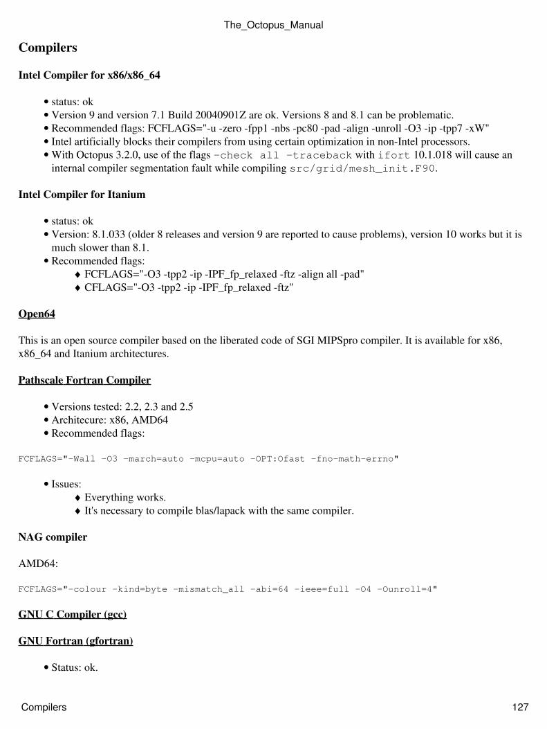
Compilers
Intel Compiler for x86/x86_64
status: ok• Version 9 and version 7.1 Build 20040901Z are ok. Versions 8 and 8.1 can be problematic.• Recommended flags: FCFLAGS="-u -zero -fpp1 -nbs -pc80 -pad -align -unroll -O3 -ip -tpp7 -xW"• Intel artificially blocks their compilers from using certain optimization in non-Intel processors.• With Octopus 3.2.0, use of the flags -check all -traceback with ifort 10.1.018 will cause aninternal compiler segmentation fault while compiling src/grid/mesh_init.F90.
•
Intel Compiler for Itanium
status: ok• Version: 8.1.033 (older 8 releases and version 9 are reported to cause problems), version 10 works but it ismuch slower than 8.1.
•
Recommended flags:FCFLAGS="-O3 -tpp2 -ip -IPF_fp_relaxed -ftz -align all -pad"♦ CFLAGS="-O3 -tpp2 -ip -IPF_fp_relaxed -ftz"♦
•
Open64
This is an open source compiler based on the liberated code of SGI MIPSpro compiler. It is available for x86,x86_64 and Itanium architectures.
Pathscale Fortran Compiler
Versions tested: 2.2, 2.3 and 2.5• Architecure: x86, AMD64• Recommended flags:•
FCFLAGS="-Wall -O3 -march=auto -mcpu=auto -OPT:Ofast -fno-math-errno"
Issues:Everything works.♦ It's necessary to compile blas/lapack with the same compiler.♦
•
NAG compiler
AMD64:
FCFLAGS="-colour -kind=byte -mismatch_all -abi=64 -ieee=full -O4 -Ounroll=4"
GNU C Compiler (gcc)
GNU Fortran (gfortran)
Status: ok.•
The_Octopus_Manual
Compilers 127
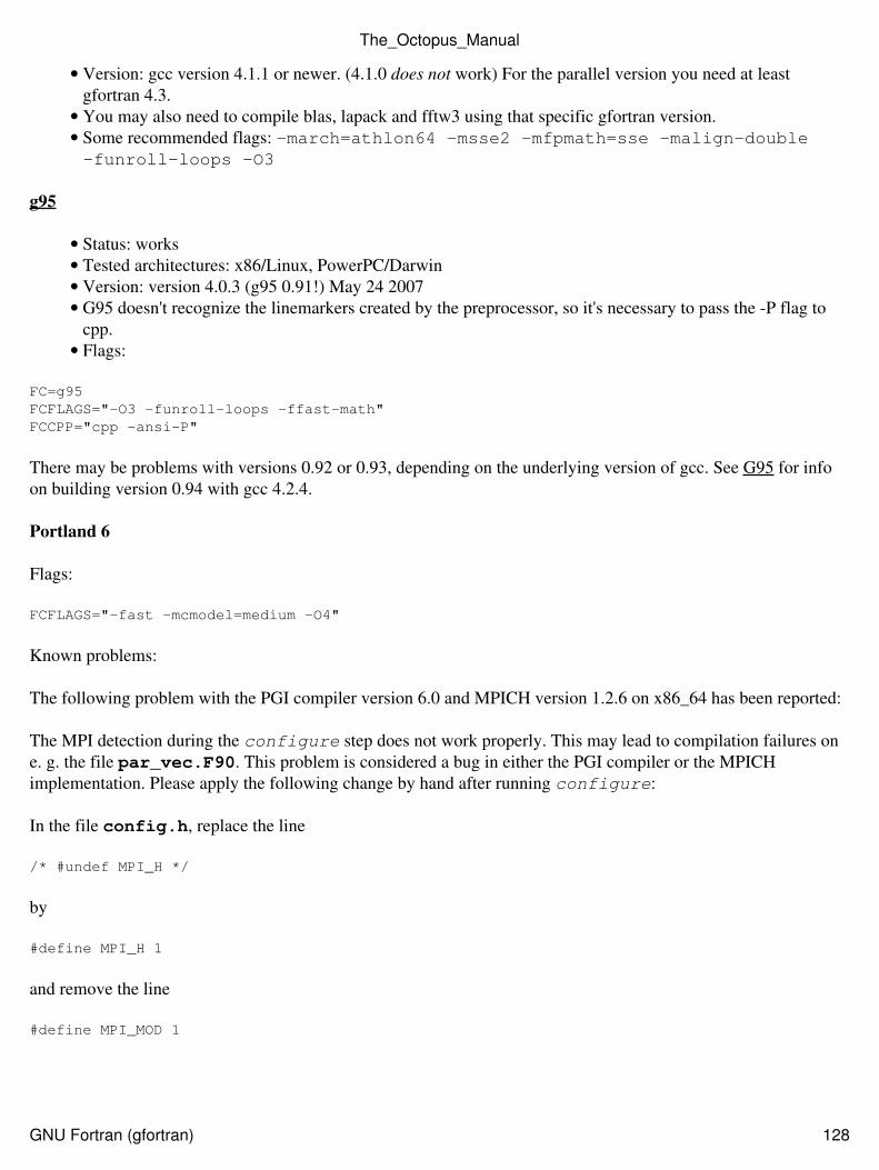
Version: gcc version 4.1.1 or newer. (4.1.0 does not work) For the parallel version you need at leastgfortran 4.3.
•
You may also need to compile blas, lapack and fftw3 using that specific gfortran version.• Some recommended flags: -march=athlon64 -msse2 -mfpmath=sse -malign-double-funroll-loops -O3
•
g95
Status: works• Tested architectures: x86/Linux, PowerPC/Darwin• Version: version 4.0.3 (g95 0.91!) May 24 2007• G95 doesn't recognize the linemarkers created by the preprocessor, so it's necessary to pass the -P flag tocpp.
•
Flags:•
FC=g95FCFLAGS="-O3 -funroll-loops -ffast-math"FCCPP="cpp -ansi-P"
There may be problems with versions 0.92 or 0.93, depending on the underlying version of gcc. See G95 for infoon building version 0.94 with gcc 4.2.4.
Portland 6
Flags:
FCFLAGS="-fast -mcmodel=medium -O4"
Known problems:
The following problem with the PGI compiler version 6.0 and MPICH version 1.2.6 on x86_64 has been reported:
The MPI detection during the configure step does not work properly. This may lead to compilation failures one. g. the file par_vec.F90. This problem is considered a bug in either the PGI compiler or the MPICHimplementation. Please apply the following change by hand after running configure:
In the file config.h, replace the line
/* #undef MPI_H */
by
#define MPI_H 1
and remove the line
#define MPI_MOD 1
The_Octopus_Manual
GNU Fortran (gfortran) 128
Portland 7, 8, 9
Flags (tested on Cray XT4):
FCFLAGS="-O2 -Munroll=c:1 -Mnoframe -Mlre -Mscalarsse -Mcache_align -Mflushz"
The configure script may fail in the part checking for Fortran libraries of mpif90 forautoconf version 2.59 or earlier. The solution is to update autoconf to 2.60 or later, or manually set FCLIBSin the configure command line to remove a spurious apostrophe.
Portland 10
For Octopus 3.2.0, the file src/basic/lookup.F90 is incorrectly optimized yielding many segmentationfaults in the testsuite. With PGI 10.5 the optimization flag should be -O2 or less; with PGI 10.8 the optimizationflag should be -O1 or less. Note that -fast and -fastsse are between -O2 and -O3. For later versions ofOctopus, a PGI pragma compels this file to be -O0 regardless of what is specified in FCFLAGS, so you may safelyset FCFLAGS to -fast.
Portland 11
11.4 does not work and will crash with glibc memory corruption errors. 11.7 is fine.
Portland 12
12.5 and 12.6 cannot compile due to an internal compiler errors of this form:
PGF90-S-0000-Internal compiler error. sym_of_ast: unexpected ast 6034 (simul_box.F90: 1103)
12.4 and 12.9 are ok.
Absoft
Flags x86:
FCFLAGS="-O3 -YEXT_NAMES=LCS -YEXT_SFX=_"
Flags amd64/em64t:
FCFLAGS="-O3 -mcmodel=medium -m64 -cpu:host -YEXT_NAMES=LCS -YEXT_SFX=_"
Compaq compiler
FCFLAGS="-align dcommons -fast -tune host -arch host -noautomatic"
Xlf
Status: works•
-bmaxdata:0x80000000 -qmaxmem=-1 -qsuffix=f=f90 -Q -O5 -qstrict -qtune=auto -qarch=auto -qhot -qipa
The_Octopus_Manual
Portland 7, 8, 9 129
Because of the exotic mixture of MAC OS and BSD, this system is not very standard. Compiling Octopuscan be problematic.
•
OS X doesn't support static linking of binaries, so don't try.•
SGI MIPS
-O3 -INLINE -n32 -LANG:recursive=on
Sun Studio
You can download this compiler for free, it supports Linux and Solaris over x86, amd64 and sparc. A very fastcompiler but quite buggy.
Flags:CFLAGS="-fast -xprefetch -xvector=simd -D__SSE2__"♦ FCFLAGS=$FLAGS♦
•
MPI Implementations
OpenMPI
MPICH2
SGI MPT
Intel MPI
Sun HPC ClusterTools
MVAPICH
NetCDF
Octopus uses the Fortran 90 interface of netCDF, this means that it's likely that you will have to compile it usingthe same compiler you will use to compile Octopus. You can get the sources and follow installation instructionsfrom the NetCDF site.
BLAS and LAPACK
These are standard libraries that provide a series of common vector and matrix operations. Octopus uses as muchas possible this libraries. There are several version available depending on your hardware. Around 40% of Octopusexecution time is spend in BLAS level 1 routines, so getting a fast implementation for your hardware might beimportant. On the other hand, Lapack performance is not very important.
The_Octopus_Manual
Xlf 130
AMD ACML
This is the AMD Mathematical Library optimized to run in Athlon and Opteron processors. You can get a freecopy from http://developer.amd.com/acml.jsp .
ATLAS
Compaq CXML
[GOTO BLAS]
Probably the fastest implementation of blas, source code is available and it can be compiled in many architectures.
Intel MKL
See https://software.intel.com/en-us/articles/intel-mkl-link-line-advisor for MKL's advice on the proper way tolink. Here is an example, in which --with-lapack is left blank because it is included in --with-blas.
MKL_DIR=/opt/intel/mkl/lib/lintel64--with-blas="-L$MKL_DIR -Wl,--start-group -lmkl_intel_lp64 -lmkl_sequential -lmkl_core -Wl,--end-group -lpthread"--with-blacs="$MKL_DIR/libmkl_blacs_intelmpi_lp64.a" --with-scalapack="$MKL_DIR/libmkl_scalapack_lp64.a"
Netlib
The reference implementation of BLAS and Lapack. It is available in most linux distributions. You can get thesource code from http://www.netlib.org/blas http://www.netlib.org/lapack .
Previous Manual:Examples:Benzene - Next Manual:Appendix:Reference Manual
Back to Manual <p class=newpage>
Appendix: Reference Manual
Variables
Previous Manual:Appendix:Porting Octopus and Platform Specific Instructions - Next Manual:Appendix:Copying
Back to Manual <p class=newpage>
Appendix: Copying
INTRODUCTION
The real-space TDDFT code octopus ("octopus") is provided under the GNU General Public License ("GPL"),Version 2, with exceptions for external libraries that are contained solely for convenience in this distribution.
You can find a copy of the GPL license here.
The_Octopus_Manual
AMD ACML 131
A copy of the exceptions and licenses follow this introduction.
LICENSE EXCEPTIONS
Octopus provides several external libraries, which are located in the "external_libs" subdirectory of the octopussource distribution. The GNU General Public License does not apply to these libraries. Separate copyright noticescan be found for each library in the respective subdirectories of "external_libs". Copyright notices are alsocontained in this document.
Currently the following external libraries are provided:
Expokit
Roger B. Sidje• Department of Mathematics, University of Queensland• Brisbane, QLD-4072, Australia• Email: [email protected]• WWW: http://www.maths.uq.edu.au/expokit/• Copyright: http://www.maths.uq.edu.au/expokit/copyright•
Metis 4.0
George Karypis• Department of Computer Science & Engineering• Twin Cities Campus• University of Minnesota, Minneapolis, MN, USA• Email: [email protected]• WWW: http://www-users.cs.umn.edu/~karypis/metis/index.html•
METIS COPYRIGHT NOTICE
The ParMETIS/METIS package is copyrighted by the Regents of the University of Minnesota. It can be freelyused for educational and research purposes by non-profit institutions and US government agencies only. Otherorganizations are allowed to use ParMETIS/METIS only for evaluation purposes, and any further uses will requireprior approval. The software may not be sold or redistributed without prior approval. One may make copies of thesoftware for their use provided that the copies, are not sold or distributed, are used under the same terms andconditions.
As unestablished research software, this code is provided on an ``as is basis without warranty of any kind, eitherexpressed or implied. The downloading, or executing any part of this software constitutes an implicit agreement tothese terms. These terms and conditions are subject to change at any time without prior notice.
qshep
Robert Renka• University of North Texas•
The_Octopus_Manual
INTRODUCTION 132
(817) 565-2767•
QSHEP COPYRIGHT NOTICE
ACM Software Copyright Notice
[3]
Copyright (c) 1998 Association for Computing Machinery, Inc. Permission to include in application software or tomake digital or hard copies of part or all of this work is subject to the following licensing agreement.
ACM Software License Agreement
All software, both binary and source published by the Association for Computing Machinery (hereafter, Software)is copyrighted by the Association (hereafter, ACM) and ownership of all right, title and interest in and to theSoftware remains with ACM. By using or copying the Software, User agrees to abide by the terms of thisAgreement.
Noncommercial Use
The ACM grants to you (hereafter, User) a royalty-free, nonexclusive right to execute, copy, modify and distributeboth the binary and source code solely for academic, research and other similar noncommercial uses, subject to thefollowing conditions:
1. User acknowledges that the Software is still in the development stage and that it is being supplied "as is,"without any support services from ACM. Neither ACM nor the author makes any representations or warranties,express or implied, including, without limitation, any representations or warranties of the merchantability or fitnessfor any particular purpose, or that the application of the software, will not infringe on any patents or otherproprietary rights of others.
2. ACM shall not be held liable for direct, indirect, incidental or consequential damages arising from any claim byUser or any third party with respect to uses allowed under this Agreement, or from any use of the Software.
3. User agrees to fully indemnify and hold harmless ACM and/or the author(s) of the original work from andagainst any and all claims, demands, suits, losses, damages, costs and expenses arising out of the User's use of theSoftware, including, without limitation, arising out of the User's modification of the Software.
4. User may modify the Software and distribute that modified work to third parties provided that: (a) if postedseparately, it clearly acknowledges that it contains material copyrighted by ACM (b) no charge is associated withsuch copies, (c) User agrees to notify ACM and the Author(s) of the distribution, and (d) User clearly notifiessecondary users that such modified work is not the original Software.
5. User agrees that ACM, the authors of the original work and others may enjoy a royalty-free, non-exclusivelicense to use, copy, modify and redistribute these modifications to the Software made by the User and distributedto third parties as a derivative work under this agreement.
The_Octopus_Manual
qshep 133
6. This agreement will terminate immediately upon User's breach of, or non-compliance with, any of its terms.User may be held liable for any copyright infringement or the infringement of any other proprietary rights in theSoftware that is caused or facilitated by the User's failure to abide by the terms of this agreement.
7. This agreement will be construed and enforced in accordance with the law of the state of New York applicableto contracts performed entirely within the State. The parties irrevocably consent to the exclusive jurisdiction of thestate or federal courts located in the City of New York for all disputes concerning this agreement.
Commercial Use
Any User wishing to make a commercial use of the Software must contact ACM at [email protected] toarrange an appropriate license. Commercial use includes (1) integrating or incorporating all or part of the sourcecode into a product for sale or license by, or on behalf of, User to third parties, or (2) distribution of the binary orsource code to third parties for use with a commercial product sold or licensed by, or on behalf of, User.
Revised 6/98
Previous Manual:Appendix:Reference Manual - Next Manual
Back to Manual
Back to Documentation
The_Octopus_Manual
QSHEP COPYRIGHT NOTICE 134