THE OCEANOGRAPHY COURSE TEAM

Authors Evelyn Brown (Waves, Tides, etc.; Ocean Chemistry) Angela Colling {Ocean Circulation; Case Studies) Dave Park (Waves, Tides, etc.) John Phillips {Case Studies) Dave Rothery {Ocean Basins) John Wright {Ocean Basins; Seawater; Ocean Chemistry; Case Studies)

Designer Jane Sheppard

Graphic Artist Sue Dobson

Cartographer Ray Munns

Editor Gerry Bearman

This Volume forms part of an Open University course. For general availability of all the Volumes in the Oceanography Series, please contact your regular supplier, or in case of difficulty the appropriate Elsevier office.

Further information on Open University courses may be obtained from: The Admissions Office, The Open University, RO. Box 48, Walton Hall, Milton Keynes MK7 6AA, UK.

Cover illustration: Satellite photograph showing distribution of phytoplankton pigments in the North Atlantic off the US coast in the region of the Gulf Stream and the Labrador Current. {NASA, and O. Brown and R. Evans, University of Miami.)

SEAWATER: ITS COMPOSITION, PROPERTIES AND BEHAVIOUR

P R E P A R E D B Y A N O P E N U N I V E R S I T Y C O U R S E T E A M

S E C O N D E D I T I O N R E V I S E D F O R T H E C O U R S E T E A M B Y

J O H N W R I G H T A N D A N G E L A C O L L I N G

P E R G A M O N

A N I M P R I N T OF E L S E V I E R SC IENCE L T D .

in assoc ia t ion w i t h

T H E O P E N U N I V E R S I T Y W A L T O N H A L L , M I L T O N K E Y N E S MK7 6AA, E N G L A N D

U K Elsevier Science Ltd, The Boulevard, Langford Lane, Kidl ington, Oxford, 0 X 5 1GB, England

U S A Elsevier Science Inc., 660 Whi te Plains Road, Tarrytown, N e w York 10591-5153, U S A

JAPAN Elsevier Science Japan, Tsunashima Building Annex, 3-20-12 Yushima, Bunkyo-ku, Tokyo 113, Japan

Copyright © 1995 The Open University

All Rights Reserved. No part of this publication may be reproduced, stored in a retrieval system or transmitted in any form or by any means: electronic, electrostatic, magnetic tape, mechanical, photocopying, recording or otherwise, without permission in writing from the copyright holders.

First edition 1989 reprinted (with corrections) 1991, 1992. Second edition 1995.

Library of Congress Cataloging in Publication Data A catalogue record for this publication is available from the Library of Congress.

British Library Cataloguing in Publication Data

A catalogue record for this publication is available from the British Library.

ISBN 0-08-0425186 (Flexicover)

Jointly published by The Open University, Walton Hall, Milton Keynes, MK7 6AA, and Pergamon, an imprint of Elsevier Science Ltd, The Boulevard, Langford Lane, Kidlington, Oxford, OX5 1GB.

Edited, typeset, illustrated and designed by The Open University.

Printed in Singapore by Kyodo under the supervision of M R M Graphics Ltd, UK.

s330v2i2.1

ABOUT THIS VOLUME

This is one of a Series of Volumes on Oceanography. It is designed so that it can be read on its own, like any other textbook, or studied as part of S330 Oceanography, a third level course for Open University students. The science of oceanography as a whole is multidisciplinary. However, different aspects fall naturally within the scope of one or other of the major 'traditional' disciplines. Thus, you will get the most out of this Volume if you have some previous experience of studying chemistry and a certain amount of physics. Other Volumes in this Series lie variously within the fields of geology, biology, physics or chemistry.

Chapter 1 summarizes the special properties of water and the role of the oceans in the hydrological cycle. Chapters 2 to 4 discuss the distribution of temperature and salinity in the oceans and their combined influence on density, stability and vertical water movements. Chapter 5 describes the behaviour of light and sound in seawater and provides examples of the application of acoustics to oceanography. Chapter 6 examines the composition and behaviour of the dissolved constituents of seawater, covering both minor and trace constituents and the major ions, as well as dissolved gases and biologically important nutrients. It deals also with such topics as residence times, speciation and carbonate equilibria. Finally, Chapter 7 provides a short review of ideas about the history of seawater, the involvement of the oceans in global cycles and their relationship to climatic change.

You will find questions designed to help you to develop arguments and/or test your own understanding as you read, with answers provided at the back of this Volume. Important technical terms are printed in bold type where they are first introduced or defined.

ABOUT THIS SERIES

The Volumes in this Series are all presented in the same style and format, and together provide a comprehensive introduction to marine science. Ocean Basins deals with structure and formation of oceanic crust, hydrothermal circulation, and factors affecting sea-level. Seawater considers the seawater solution and leads naturally into Ocean Circulation, the ' core ' of the Series, providing a largely non-mathematical treatment of ocean-atmosphere interaction and the dynamics of wind-driven surface current systems, and of density-driven circulation in the deep oceans. Waves, Tides and Shallow-Water Processes introduces processes controlling water movement and sediment transport in nearshore environments (beaches, estuaries, deltas, shelves). Ocean Chemistry and Deep-Sea Sediments is concerned with biogeochemical cycling of elements within the seawater solution and with water-sediment interaction on the ocean floor. Case Studies in Oceanography and Marine Affairs examines the effect of human intervention in the marine environment and introduces the essentials of Law of the Sea. The two interdisciplinary case studies respectively review marine affairs in the Arctic from an historical standpoint, and outline the causes and effects of the tropical climatic phenomenon known as El Nino.

Biological Oceanography: An Introduction (by C. M. Lalli and T. R. Parsons) is a companion Volume to the Series, and is also in the same style and format. It describes and explains interactions between marine plants and animals in relation to the physical/chemical properties and dynamic behaviour of the seawater in which they live.

ABOUT THIS VOLUME

This is one of a Series of Volumes on Oceanography. It is designed so that it can be read on its own, like any other textbook, or studied as part of S330 Oceanography, a third level course for Open University students. The science of oceanography as a whole is multidisciplinary. However, different aspects fall naturally within the scope of one or other of the major 'traditional' disciplines. Thus, you will get the most out of this Volume if you have some previous experience of studying chemistry and a certain amount of physics. Other Volumes in this Series lie variously within the fields of geology, biology, physics or chemistry.

Chapter 1 summarizes the special properties of water and the role of the oceans in the hydrological cycle. Chapters 2 to 4 discuss the distribution of temperature and salinity in the oceans and their combined influence on density, stability and vertical water movements. Chapter 5 describes the behaviour of light and sound in seawater and provides examples of the application of acoustics to oceanography. Chapter 6 examines the composition and behaviour of the dissolved constituents of seawater, covering both minor and trace constituents and the major ions, as well as dissolved gases and biologically important nutrients. It deals also with such topics as residence times, speciation and carbonate equilibria. Finally, Chapter 7 provides a short review of ideas about the history of seawater, the involvement of the oceans in global cycles and their relationship to climatic change.

You will find questions designed to help you to develop arguments and/or test your own understanding as you read, with answers provided at the back of this Volume. Important technical terms are printed in bold type where they are first introduced or defined.

ABOUT THIS SERIES

The Volumes in this Series are all presented in the same style and format, and together provide a comprehensive introduction to marine science. Ocean Basins deals with structure and formation of oceanic crust, hydrothermal circulation, and factors affecting sea-level. Seawater considers the seawater solution and leads naturally into Ocean Circulation, the ' core ' of the Series, providing a largely non-mathematical treatment of ocean-atmosphere interaction and the dynamics of wind-driven surface current systems, and of density-driven circulation in the deep oceans. Waves, Tides and Shallow-Water Processes introduces processes controlling water movement and sediment transport in nearshore environments (beaches, estuaries, deltas, shelves). Ocean Chemistry and Deep-Sea Sediments is concerned with biogeochemical cycling of elements within the seawater solution and with water-sediment interaction on the ocean floor. Case Studies in Oceanography and Marine Affairs examines the effect of human intervention in the marine environment and introduces the essentials of Law of the Sea. The two interdisciplinary case studies respectively review marine affairs in the Arctic from an historical standpoint, and outline the causes and effects of the tropical climatic phenomenon known as El Nino.

Biological Oceanography: An Introduction (by C. M. Lalli and T. R. Parsons) is a companion Volume to the Series, and is also in the same style and format. It describes and explains interactions between marine plants and animals in relation to the physical/chemical properties and dynamic behaviour of the seawater in which they live.

CHAPTER 1 WATER, AIR AND ICE

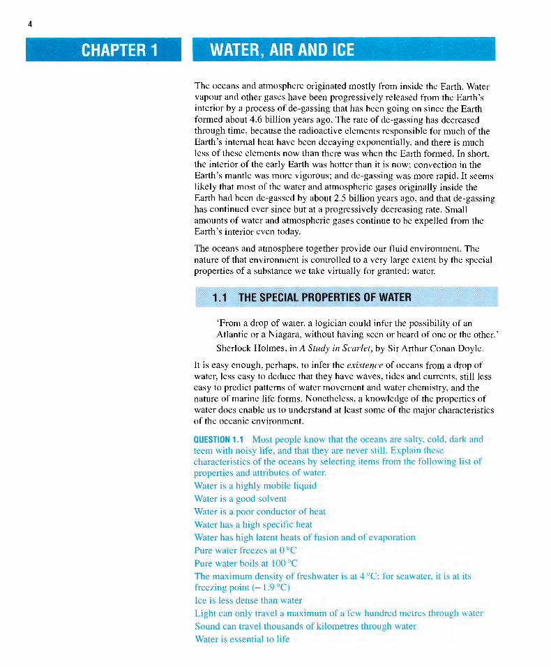
The oceans and atmosphere originated mostly from inside the Earth. Water vapour and other gases have been progressively released from the Earth's interior by a process of de-gassing that has been going on since the Earth formed about 4.6 billion years ago. The rate of de-gassing has decreased through time, because the radioactive elements responsible for much of the Earth's internal heat have been decaying exponentially, and there is much less of these elements now than there was when the Earth formed. In short, the interior of the early Earth was hotter than it is now; convection in the Earth's mantle was more vigorous; and de-gassing was more rapid. It seems likely that most of the water and atmospheric gases originally inside the Earth had been de-gassed by about 2.5 billion years ago, and that de-gassing has continued ever since but at a progressively decreasing rate. Small amounts of water and atmospheric gases continue to be expelled from the Earth's interior even today.

The oceans and atmosphere together provide our fluid environment. The nature of that environment is controlled to a very large extent by the special properties of a substance we take virtually for granted: water.

1.1 THE SPECIAL PROPERTIES OF WATER

'From a drop of water, a logician could infer the possibility of an Atlantic or a Niagara, without having seen or heard of one or the other.'

Sherlock Holmes, in A Study in Scarlet, by Sir Arthur Conan Doyle.

It is easy enough, perhaps, to infer the existence of oceans from a drop of water, less easy to deduce that they have waves, tides and currents, still less easy to predict patterns of water movement and water chemistry, and the nature of marine life forms. Nonetheless, a knowledge of the properties of water does enable us to understand at least some of the major characteristics of the oceanic environment.

Q U E S T I O N 1.1 Most people know that the oceans are salty, cold, dark and teem with noisy life, and that they are never still. Explain these characteristics of the oceans by selecting items from the following list of

properties and attributes of water.

Water is a highly mobile liquid

Water is a good solvent

Water is a poor conductor of heat

Water has a high specific heat

Water has high latent heats of fusion and of evaporation

Pure water freezes at 0 °C

Pure water boils at 10()°C

The maximum density of freshwater is at 4 °C; for seawater, it is at its

freezing point ( - 1.9 °C)

Ice is less dense than water

Light can only travel a maximum of a few hundred metres through water

Sound can travel thousands of kilometres through water

Water is essential to life

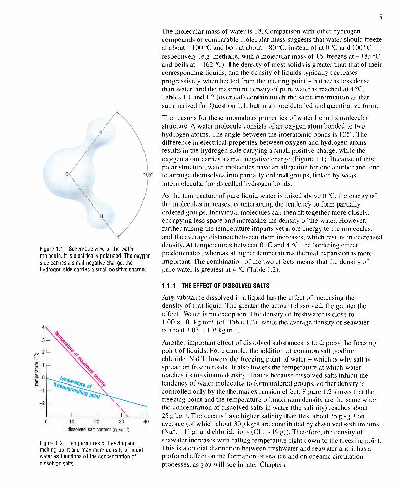
Figure 1.1 Schematic view of the water molecule. It is electrically polarized. The oxygen side carries a small negative charge; the hydrogen side carries a small positive charge.

4 f r

10 20 30

dissolved salt content {g kg~ 40

Figure 1.2 Temperatures of freezing and melting point and maximum density of liquid water as functions of the concentration of dissolved salts.

The molecular mass of water is 18. Comparison with other hydrogen compounds of comparable molecular mass suggests that water should freeze at about - 100 °C and boil at about - 80 °C, instead of at 0 °C and 100 °C respectively (e.g. methane, with a molecular mass of 16, freezes at - 183 °C and boils at - 162 °C). The density of most solids is greater than that of their corresponding liquids, and the density of liquids typically decreases progressively when heated from the melting point - but ice is less dense than water, and the maximum density of pure water is reached at 4 °C. Tables 1.1 and 1.2 (overleaf) contain much the same information as that summarized for Question 1.1, but in a more detailed and quantitative form.

The reasons for these anomalous properties of water lie in its molecular structure. A water molecule consists of an oxygen atom bonded to two hydrogen atoms. The angle between the interatomic bonds is 105°. The difference in electrical properties between oxygen and hydrogen atoms results in the hydrogen side carrying a small positive charge, while the oxygen atom carries a small negative charge (Figure 1,1). Because of this polar structure, water molecules have an attraction for one another and tend to arrange themselves into partially ordered groups, linked by weak intermolecular bonds called hydrogen bonds.

As the temperature of pure liquid water is raised above 0 °C, the energy of the molecules increases, counteracting the tendency to form partially ordered groups. Individual molecules can then fit together more closely, occupying less space and increasing the density of the water. However, further raising the temperature imparts yet more energy to the molecules, and the average distance between them increases, which results in decreased density. At temperatures between 0 °C and 4 °C, the 'ordering effect' predominates, whereas at higher temperatures thermal expansion is more important. The combination of the two effects means that the density of pure water is greatest at 4 °C (Table 1.2).

1.1.1 T H E E F F E C T OF D I S S O L V E D S A L T S

Any substance dissolved in a liquid has the effect of increasing the density of that liquid. The greater the amount dissolved, the greater the effect. Water is no exception. The density of freshwater is close to 1.00 X 103 k g m - 3 (cf. Table 1.2), while the average density of seawater is about 1.03 x 10^ k g m - 3 .

Another important effect of dissolved substances is to depress the freezing point of liquids. For example, the addition of common salt (sodium chloride, NaCl) lowers the freezing point of water - which is why salt is spread on frozen roads. It also lowers the temperature at which water reaches its maximum density. That is because dissolved salts inhibit the tendency of water molecules to form ordered groups, so that density is controlled only by the thermal expansion effect. Figure 1.2 shows that the freezing point and the temperature of maximum density are the same when the concentration of dissolved salts in water (the salinity) reaches about 25 g k g - ' . The oceans have higher salinity than this, about 35 gkg- i on average (of which about 3 0 g k g - i are contributed by dissolved sodium ions (Na^, ~ 11 g) and chloride ions (CI", ~ 19 g)). Therefore, the density of seawater increases with falling temperature right down to the freezing point. This is a crucial distinction between freshwater and seawater and it has a profound effect on the formation of sea-ice and on oceanic circulation processes, as you will see in later Chapters.

5

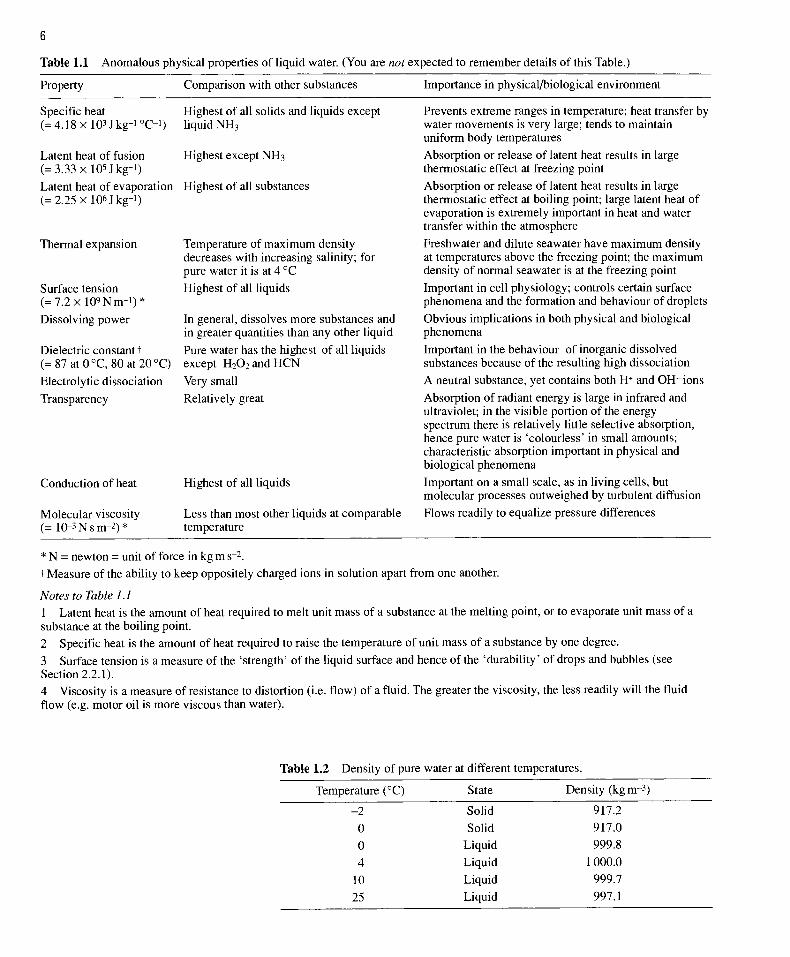
Table 1.1 Anomalous physical properties of liquid water. (You are not expected to remember details of this Table.)

Property Comparison with other substances Importance in physical/biological environment

Specific heat (= 4.18X 103Jkg-i °C-i)

Highest of all solids and liquids except liquid NH3

Latent heat of fusion Highest except NH3 (=3 .33x l05Jkg- i )

Latent heat of evaporation Highest of all substances (= 2.25 X 106Jkg-i)

Thermal expansion

Surface tension ( = 7 . 2 x l 0 9 N m - i ) * Dissolving power

Dielectric constant t (= 87atO°C, 80 at 20 °C)

Electrolytic dissociation

Transparency

Temperature of maximum density decreases with increasing salinity; for pure water it is at 4 °C

Highest of all liquids

In general, dissolves more substances and in greater quantities than any other liquid

Pure water has the highest of all liquids except H202andHCN

Very small

Relatively great

Conduction of heat

Molecular viscosity (= 10-3Nsm-2)*

Highest of all liquids

Less than most other liquids at comparable temperature

Prevents extreme ranges in temperature; heat transfer by water movements is very large; tends to maintain uniform body temperatures

Absorption or release of latent heat results in large thermostatic effect at freezing point

Absorption or release of latent heat results in large thermostatic effect at boiling point; large latent heat of evaporation is extremely important in heat and water transfer within the atmosphere

Freshwater and dilute seawater have maximum density at temperatures above the freezing point; the maximum density of normal seawater is at the freezing point

Important in cell physiology; controls certain surface phenomena and the formation and behaviour of droplets

Obvious implications in both physical and biological phenomena

Important in the behaviour of inorganic dissolved substances because of the resulting high dissociation

A neutral substance, yet contains both H+ and OH- ions

Absorption of radiant energy is large in infrared and ultraviolet; in the visible portion of the energy spectrum there is relatively little selective absorption, hence pure water is 'colourless' in small amounts; characteristic absorption important in physical and biological phenomena

Important on a small scale, as in living cells, but molecular processes outweighed by turbulent diffusion

Flows readily to equalize pressure differences

* N = newton = unit of force in kg m s-2.

t Measure of the ability to keep oppositely charged ions in solution apart from one another.

Notes to Table 1J 1 Latent heat is the amount of heat required to melt unit mass of a substance at the melting point, or to evaporate unit mass of a substance at the boiling point. 2 Specific heat is the amount of heat required to raise the temperature of unit mass of a substance by one degree.

3 Surface tension is a measure of the 'strength' of the liquid surface and hence of the 'durability' of drops and bubbles (see Section 2.2.1). 4 Viscosity is a measure of resistance to distortion (i.e. flow) of a fluid. The greater the viscosity, the less readily will the fluid flow (e.g. motor oil is more viscous than water).

Table 1.2 Density of pure water at different temperatures.

Temperature (°C) State Density (kg nr^)

-2 Solid 917.2

0 Solid 917.0

0 Liquid 999.8

4 Liquid I 000.0

10 Liquid 999.7

25 Liquid 997.1

6

Q U E S T I O N 1.2 On Figure 1.2 (p. 5), do the words ^maximum density' refer to a single density value, or does the maximum density itself increase or decrease along the line, with falling temperature and increasing dissolved salt content?

1.2 THE HYDROLOGICAL CYCLE

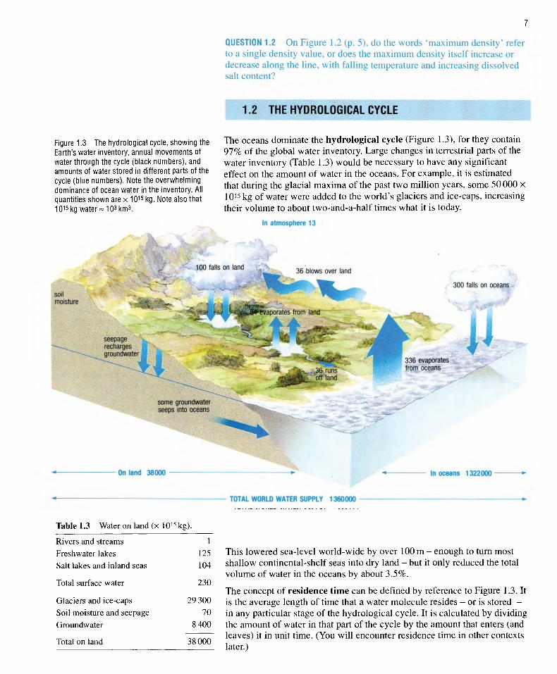
Figure 1.3 The hydrological cycle, showing the Earth's water inventory, annual movements of water through the cycle (black numbers), and amounts of water stored in different parts of the cycle (blue numbers). Note the overwhelming dominance of ocean water in the inventory. All quantities shown are x 10^5 kg. Note also that 1 0 1 5 k g w a t e r - 1 0 3 k m 3 .

The oceans dominate the hydrological cycle (Figure 1.3), for they contain 97% of the global water inventory. Large changes in terrestrial parts of the water inventory (Table 1.3) would be necessary to have any significant effect on the amount of water in the oceans. For example, it is estimated that during the glacial maxima of the past two million years, some 50000 x 1015 kg of water were added to the world's glaciers and ice-caps, increasing their volume to about two-and-a-half times what it is today.

In atmosphere 13

36 blows over land

300 falls on oceans

On land 38000 In oceans 1322000

TOTAL WORLD WATER SUPPLY 1360000

Table 1.3 Water on land (x IQis kg).

Rivers and streams 1

Freshwater lakes 125

Salt lakes and inland seas 104

Total surface water 230

Glaciers and ice-caps 29 300

Soil moisture and seepage 70

Groundwater 8400

Total on land 38 000

This lowered sea-level world-wide by over 100 m - enough to turn most shallow continental-shelf seas into dry land - but it only reduced the total volume of water in the oceans by about 3.5%.

The concept of residence time can be defined by reference to Figure 1.3. It is the average length of time that a water molecule resides - or is stored -in any particular stage of the hydrological cycle. It is calculated by dividing the amount of water in that part of the cycle by the amount that enters (and leaves) it in unit time. (You will encounter residence time in other contexts later.)

7

Q U E S T I O N 1.3 (a) Look ai Figure 1.3. Whai is the annual rate of evaporation from the ocean? Is it balanced by [irecipilation plus run-olT from land?

i b ) VVlial is the residence time ol water in the oceans?

(e) Approximately vviiat cjuantity ol water moves through the atmosphere M i j i i u a l l y */

1.2.1 W A T E R IN T H E A T M O S P H E R E

The most obvious manifestations of water in the atmosphere are clouds and fog. Both consist of water droplets or ice crystals that have condensed round (or nucleated on) small particles in the air. Water in the atmosphere is mostly in the gaseous state, i.e. as water vapour. Air is saturated with water vapour when there is equilibrium between evaporation and condensation. The higher the temperature, the greater the amount of energy available for evaporation, so warm air can hold more moisture at saturation (i.e. it has higher humidity) than cold air.

There are two ways in which unsaturated air can be cooled so that it becomes saturated and condensation begins:

1 Cooling occurs when air rises and expands adiabatically as atmospheric pressure decreases with height. Adiabatic changes of temperature are those that occur independently of any transfer of heat to or from the surroundings (see also Section 4.2.1). Thus, rising air expands and loses internal energy, so that its temperature may fall sufficiently for the water vapour it contains to condense as water droplets and form cloud or fog.

2 Cooling also occurs when air comes into contact with a cold surface (which is why you get condensation on windows in winter, for example). Fogs develop when a sufficiently thick layer of moist air is cooled to condensation point, forming in effect clouds at ground (or water) level. Two main types of fog are recognized.

Radiation fog forms when the ground surface is cooled by radiant heat loss at night into a clear sky. If the air in contact with the ground is close to saturation and its temperature falls sufficiently, then fog may form. Radiation fogs do not develop over lakes or the sea, because water has a high specific heat (Table 1.1), so water surfaces cool less rapidly than ground surfaces. However, radiation fog often drifts from land over rivers, estuaries and coastal waters.

Advection fog forms when warm humid air moves (is advected) over cold ground or water and is cooled. Such fogs commonly develop over the Grand Banks off Newfoundland for example, where air formerly above the warm Gulf Stream is advected over the cold Labrador Current (see Figure 2.11).

1.2.2 ICE IN T H E O C E A N S

Polar ice-caps are a significant feature of the present-day Earth. A layer of ice with its covering of snow reflects back more incoming solar radiation than areas of land or open water (see Section 2.1). Only a small amount of solar energy can penetrate to surface water or land under the ice, so that once it is established, ice tends to be self-perpetuating.

Sea-ice is formed by the freezing of seawater itself. Various stages and ages of sea-ice formation are illustrated in Figure 1.4. When seawater first begins to freeze, relatively pure ice is formed, so that the salt content of the surrounding seawater is increased, which both increases its density and depresses its freezing point further (cf. Figure 1.2). Most of the salt in sea-ice is in the form of concentrated brine droplets trapped within the ice as it forms. Brine trapped

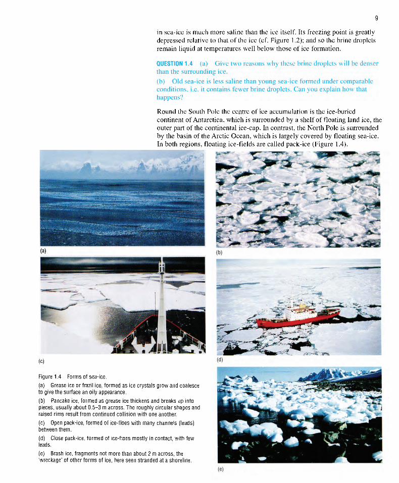
in sea-ice is much more saUne than the ice itself. Its freezing point is greatly depressed relative to that of the ice (cf. Figure 1.2); and so the brine droplets remain liquid at temperatures well below those of ice formation.

Q U E S T I O N 1.4 (a) (lixc two reasons \vh\ these brine droplets will be Denver than the siirroiinclinii iee.

(b) Old sea-iee is less salnie than voiinii ^ea-iee loniied iinclei ei>niparabie eoiiditions, i.e. it eontains fewer brine droplets, (du xou explain liow tluit happens?

Round the South Pole the centre of ice accumulation is the ice-buried continent of Antarctica, which is surrounded by a shelf of floating land ice, ihe outer part of the continental ice-cap. In contrast, the North Pole is surrounded by the basin of the Arctic Ocean, which is largely covered by floating sea-ice. In both regions, floating ice-fields are called pack-ice (Figure 1.4).

Figure 1.4 Forms of sea-ice.

(a) Grease ice or frazil ice, formed as ice crystals grow and coalesce to give the surface an oily appearance.

(b) Pancake ice, formed as grease ice thickens and breaks up into pieces, usually about 0.5-3 m across. The roughly circular shapes and raised rims result f rom continued collision with one another.

(c) Open pack-ice, formed of ice-floes with many channels (leads) between them.

(d) Close pack-ice, formed of ice-floes mostly in contact, with few leads.

(e) Brash ice, fragments not more than about 2 m across, the 'wreckage' of other forms of ice, here seen stranded at a shoreline.

9

10

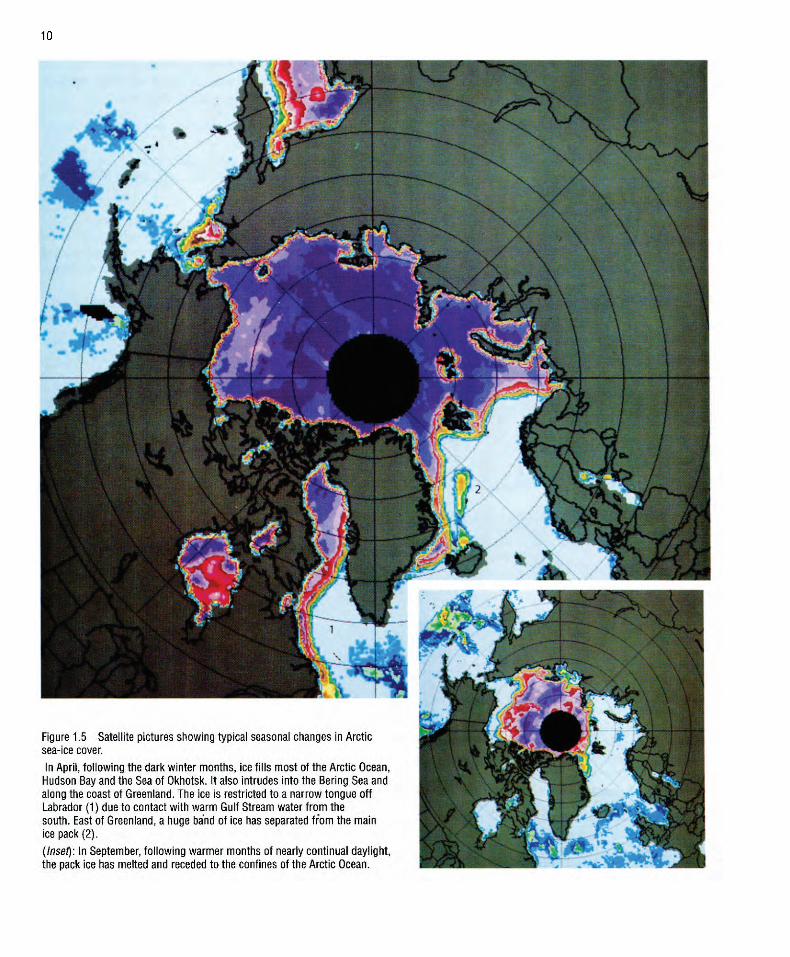
Figure 1.5 Satellite pictures showing typical seasonal changes in Arctic sea-ice cover.

In April, following the dark winter months, ice fills most of the Arctic Ocean, Hudson Bay and the Sea of Okhotsk. It also intrudes into the Bering Sea and along the coast of Greenland. The ice is restricted to a narrow tongue off Labrador (1) due to contact with warm Gulf Stream water f rom the south. East of Greenland, a huge band of ice has separated from the main ice pack (2).

(Inset): In September, following warmer months of nearly continual daylight, the pack ice has melted and receded to the confines of the Arctic Ocean.

11

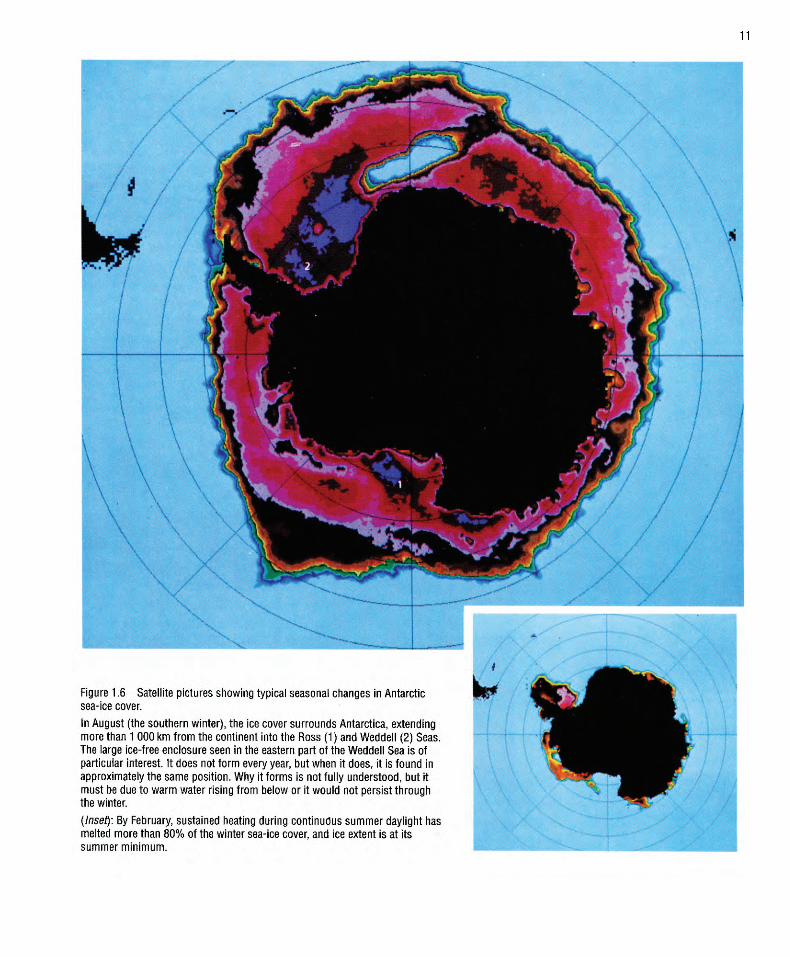
Figure 1.6 Satellite pictures showing typical seasonal changes in Antarctic sea-ice cover.

In August (the southern winter), the ice cover surrounds Antarctica, extending more than 1 000 km from the continent into the Ross (1) and Weddell (2) Seas. The large ice-free enclosure seen in the eastern part of the Weddell Sea is of particular interest. It does not form every year, but when it does, it is found in approximately the same position. W h y it forms is not fully understood, but it must be due to warm water rising from below or it would not persist through the winter.

(Inset): By February, sustained heating during continuous summer daylight has melted more than 80% of the winter sea-ice cover, and ice extent is at its summer minimum.

12

Seasonal and inter-annual changes in ice cover at high latitudes are monitored by satellite (Figures 1.5 and 1.6). A knowledge of the extent of ice cover and the way it changes with time is crucial to understanding and predicting weather patterns and such data are important for assessing the surface radiation balance of the Earth as a whole.

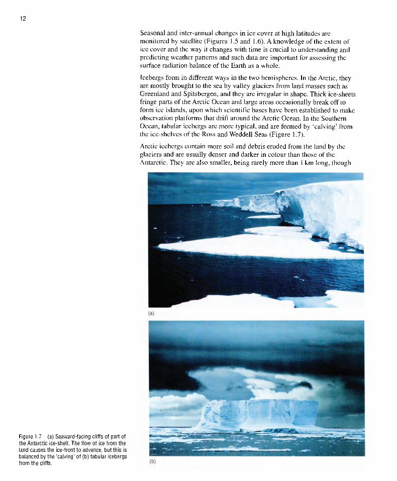
Icebergs form in different ways in the two hemispheres. In the Arctic, they are mostly brought to the sea by valley glaciers from land masses such as Greenland and Spitsbergen, and they are irregular in shape. Thick ice-sheets fringe parts of the Arctic Ocean and large areas occasionally break off to form ice islands, upon which scientific bases have been estabhshed to make observation platforms that drift around the Arctic Ocean. In the Southern Ocean, tabular icebergs are more typical, and are formed by 'calving' from the ice-shelves of the Ross and Weddell Seas (Figure 1.7).

Arctic icebergs contain more soil and debris eroded from the land by the glaciers and are usually denser and darker in colour than those of the Antarctic. They are also smaller, being rarely more than 1 km long, though

Figure 1.7 (a) Seaward-facing cliffs of part of the Antarctic ice-shelf. The flow of ice from the land causes the ice-front to advance, but this is balanced by the 'calving' of (b) tabular icebergs from the cliffs.

13

1.3 SUMMARY OF CHAPTER 1

1 The special properties of water - in particular, its anomalously high melting and boiling points, specific and latent heats, powerful solvent properties, and maximum density at 4 °C - result from the polar structure of the water molecule. Dissolved salts increase the density of water and depress both the temperature of maximum density and the freezing point.

2 The oceans contain 97% of the water that circulates in the hydrological cycle. The residence time of water in the oceans is measured in thousands of years; in the atmosphere, it is measured in days.

3 Air is saturated with water vapour when evaporation is balanced by condensation. Clouds and fog are condensed water vapour. Fog niay form when air is cooled to its condensation temperature, either by radiation from the land, or by advection of warm humid air over a cool land or water surface.

4 Sea-ice is less saline than the seawater from which it freezes, so its formation increases the salt content of the remaining seawater, thus further depressing its freezing point and increasing its density. Icebergs in the Northern Hemisphere are formed when valley glaciers on lands surrounding the Arctic Ocean reach the sea; those in the Southern Hemisphere break off from the thick ice-shelf that surrounds the Antarctic continent.

Now try the following questions to consolidate your understanding of this

Chapter.

Q U E S T I O N 1.5 (a) hi what ways are the thermal properties o f watei

probably the single most important factor in preventing extremes o f temperature from being reached at the Fiartli's surface'?

(b) Most liquids reach a maxinuun density at IVee/ing point, but p u i . w d i e i is an exception. At what temperature does pure water reach n m x n n u n i density? Does this temperature apply to seawater/

Q U E S T I O N 1.6 What is the approximate average residence lime o l w a l e i o i i land, and \ \h \ is this average \a lue likely to conceal considerable v a r K i n o i i N

Q U E S T I O N 1.7 (a) What is the man] ciirierence in oniini b e t w e e n (hi u sheets that cover the Arctic and Antarctic polar legions

(b) A sample of water contains 20g kg ' d issoheel salts. A l w h i i temperature will it (i) attain its maximum density, (ii) IVee/e?

(c) ice melts and mixes with seawater of salinity 3^ g kg W i l l t in - h a w the effect of raising or lowering the freezing point of ihe seawaiei? W o u i v i this in turn tend to facilitate the formation of moie sea-ice w h e ! i l en ip i i ; n i M e • fell once more?

they can be as high as 60 m above the sea-surface. Antarctic icebergs may have surface areas of many square kilometres, but they are rarely more than 35 m high. As icebergs melt, they dilute the surface seawater with freshwater, and the salinity of surface seawater in high latitudes is appreciably less than in ice-free latitudes: about 30 -33 g k g - i , as against 35 gkg - i .

The next Chapter is concerned with the distribution of temperature in the oceans and some of the reasons for that distribution.

14

CHAPTER 2 TEMPERATURE IN THE OCEANS

Two of the most important properties of seawater are temperature and salinity (concentration of dissolved salts), for together they control its density, which is the major factor governing the vertical movement of ocean waters.

In the oceans, the density of seawater normally increases with depth. If the density of surface water exceeds that of the underlying water, the situation is gravitationally unstable and the surface water sinks. In polar regions, the density of surface waters can be increased in two ways: first, by direct cooling, either where ice is in contact with the water or where cold winds blow off the ice; secondly, by the formation of sea-ice, which extracts water and leaves behind seawater of higher salinity and increased density (Section 1.2.2). The cold dense currents of the deep circulation (see Section 4.1) originate by sinking of dense water in polar regions. In lower latitudes, dense saline water is produced by excess evaporation, which may be aided by strong winds such as those that occur during the winter in parts of the Mediterranean.

2.1 SOLAR RADIATION

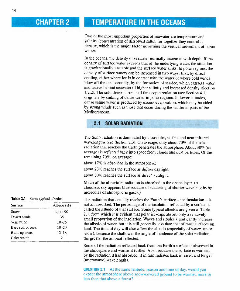
Table 2.1 Some typical albedos.

Surface Albedo (%)

Snow up to 90

Desert sands 35 Vegetation 10-25

Bare soil or rock 10-20

Built-up areas 12-18 Calm water 2

The Sun's radiation is dominated by ultraviolet, visible and near infrared wavelengths (see Section 2.3). On average, only about 70% of the solar radiation that reaches the Earth penetrates the atmosphere. About 30% (on average) is reflected back into space from clouds and dust particles. Of the remaining 70%, on average:

about 17% is absorbed in the atmosphere;

about 2 3 % reaches the surface as diffuse daylight;

about 30% reaches the surface as direct sunlight.

Much of the ultraviolet radiation is absorbed in the ozone layer. (A cloudless sky appears blue because of scattering of shorter wavelengths by molecules of atmospheric gases.)

The radiation that actually reaches the Earth's surface - the insolation - is not all absorbed. The percentage of the insolation reflected by a surface is called the albedo of that surface. Some typical albedos are given in Table 2.1 , from which it is evident that polar ice-caps absorb only a relatively small proportion of the insolation. Waves and ripples significantly increase the albedo of water, but it is still generally less than that of most surfaces on land. The time of day will also affect the albedo (especially of water, ice or snow), because the shallower the angle of incidence of the solar radiation the greater the amount reflected.

Some of the radiation reflected back from the Earth's surface is absorbed in the atmosphere and warms it further. Also, because the surface is warmed by the radiation it has absorbed, it in turn radiates back infrared and longer (microwave) wavelengths.

Q U E S T I O N 2.1 At the same latitude, season and time of day, would you expect the atmosphere above snow-covered ground to be warmed more or less than that above a forest?

15

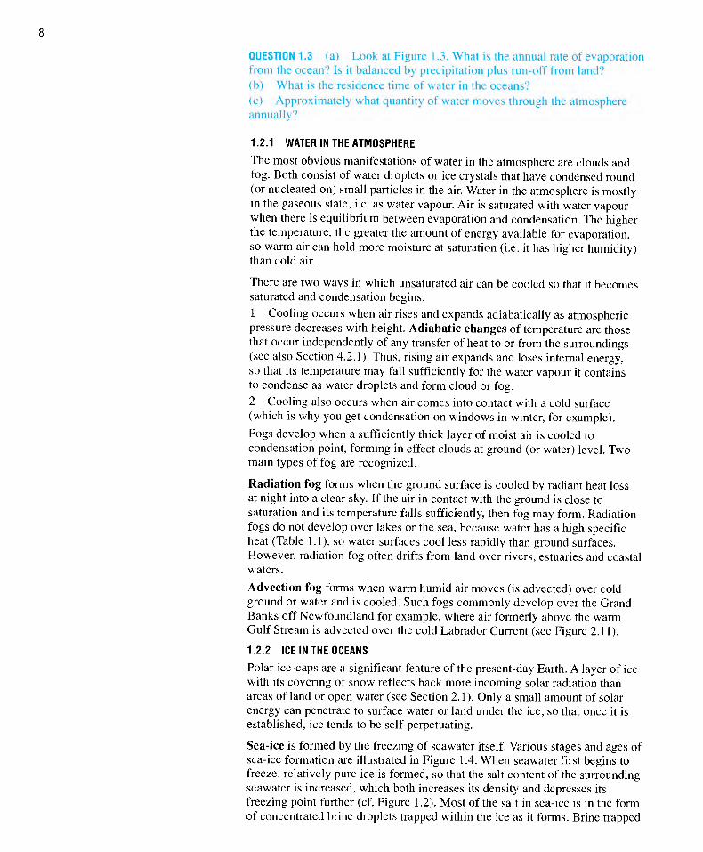
highest recorded air temperature (Libya, 1922)

3D

22 20

10

lower observed limit, breeding range of Emperor penguin (-18 to-62)

lowest recorded air temperature (Siberia, 1892)

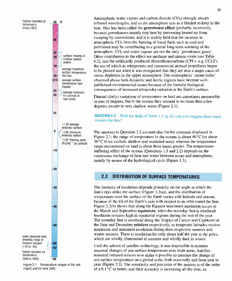
Figure 2.1 Temperature ranges in the sea (right) and on land (left).

-1.33 average Antarctic surface

|=/-1.65 minimum, "^Antarctic bottom

-1.87 freezing point, 35 g kg"^ (at surface)

-10

-20

H30

-40

surface maxima in y shallow coastal

waters

average maximum surface temperature,

- Red Sea - average surface

temperature near Equator

" \ average minimum "-̂ for survival of

reef corals

Atmospheric water vapour and carbon dioxide (CO2) strongly absorb infrared wavelengths, and so the atmosphere acts as a blanket to keep in the heat. This has been called the greenhouse effect (probably incorrectly, because greenhouses mainly trap heat by preventing heated air from escaping by convection), and it is widely held that the increase in atmospheric CO2 from the burning of fossil fuels such as coal and petroleum may be contributing to a general long-term warming of the atmosphere. CO2 and water vapour are not the only 'greenhouse gases ' . Other contributors to the effect are methane and nitrous oxide (see Table 6.2), and the artificially produced chlorofluorocarbons (CFCs, e.g. CCI3F), the use of which as refrigerants and commercial aerosol propellants began to be phased out when it was recognized that they are also a major cause of ozone depletion in the upper atmosphere. The stratospheric 'ozone holes ' observed above both Antarctic and Arctic regions have become well-publicized environmental issues because of the harmful biological consequences of increased ultraviolet radiation at the Earth's surface.

Diurnal (daily) variations of temperature on land are sometimes measurable in tens of degrees, but in the oceans they amount to no more than a few degrees, except in very shallow water (Figure 2.1).

Q U E S T I O N 2.2 With the help of Table 1.1 (p. 6), can you suggest three main reasons for this?

The answers to Question 2.2 account also for the contrasts displayed in Figure 2 .1: the range of temperature in the oceans is about 40 °C (or about 30 °C if we exclude shallow and restricted seas); whereas the temperature range encountered on land is about three times greater. The temperature-buffering effect of the oceans (Questions 1.5 and 2.2) depends on the continuous exchange of heat and water between ocean and atmosphere, mainly by means of the hydrological cycle (Figure 1.3).

2.2 DISTRIBUTION OF SURFACE TEMPERATURES

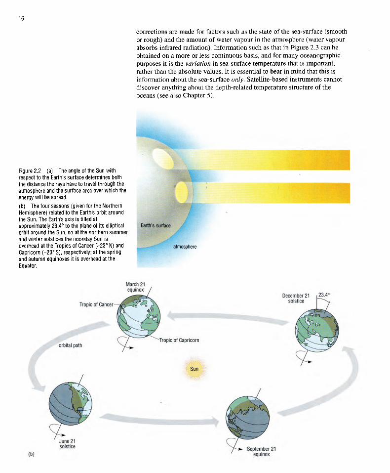
The intensity of insolation depends primarily on the angle at which the Sun's rays strike the surface (Figure 2.2(a)), and the distribution of temperature over the surface of the Earth varies with latitude and season, because of the tilt of the Earth's axis with respect to its orbit round the Sun. Figure 2.2(b) shows that along the Equator maximum insolation occurs at the March and September equinoxes, when the noonday Sun is overhead. Insolation remains high in equatorial regions during the rest of the year. The noonday Sun is overhead along the Tropics of Cancer and Capricorn at the June and December solstices respectively, so temperate latitudes receive maximum and minimum insolation during their respective summer and winter seasons. There is insolation for only about half the year at the poles, which are wholly illuminated in summer and wholly dark in winter.

Until the advent of satellite technology, it was impossible to monitor seasonal changes of sea-surface temperature over wide areas. Satellite-mounted infrared sensors now make it possible to measure the change of sea-surface temperature on a global scale, both seasonally and from year to year (Figure 2.3). The sensitivity and precision of the sensors is of the order of ±0 .1 °C or better, and their accuracy is increasing all the time, as

58 %

m

0

16

corrections are made for factors such as the state of the sea-surface (smooth or rough) and the amount of water vapour in the atmosphere (water vapour absorbs infrared radiation). Information such as that in Figure 2.3 can be obtained on a more or less continuous basis, and for many oceanographic purposes it is the variation in sea-surface temperature that is important, rather than the absolute values. It is essential to bear in mind that this is information about the sea-surface only. Satellite-based instruments cannot discover anything about the depth-related temperature structure of the oceans (see also Chapter 5).

Figure 2.2 (a) The angle of the Sun with respect to the Earth's surface determines both the distance the rays have to travel through the atmosphere and the surface area over which the energy will be spread.

(b) The four seasons (given for the Northern Hemisphere) related to the Earth's orbit around the Sun. The Earth's axis Is tilted at approximately 23.4° to the plane of its elliptical orbit around the Sun, so at the northern summer and winter solstices the noonday Sun is overhead at the Tropics of Cancer (-23'' N) and Capricorn (-23° S) , respectively; at the spring and autumn equinoxes it is overhead at the Equator.

Earth's surface

atmosphere

(a)

March 21 equinox

Tropic of Cancer

orbital path

December 21 L23-4° solstice

Tropic of Capricorn

Sun

June 21 solstice

(b) September 21

equinox

17

Figure 2.3 Daytime sea-surface temperature measurements from satellite-borne sensors. For the upper two pictures, temperatures below 0 °C are green and blue; higher temperatures are red and brown.

(Top): In January, the Northern Hemisphere experiences extreme cold. In Siberia and over most of Canada, temperatures approach -30 °C, while in Eastern Europe and the northern USA temperatures are below 0 °C. In the Southern Hemisphere it is summer, with mid-latitude temperatures ranging from 20 °C to 30 °C. On the eastern and western sides of the major oceans, the contours of equal temperature show deviations from their latitudinal (or zonal) patterns. Generally, in the sub-tropics of both hemispheres (c. 10° to 30°), the western sides of the oceans are warmer than their eastern counterparts, primarily due to ocean currents. The Gulf Stream can be seen moving along the eastern North American coast, then turning eastwards and transporting warm waters across the Atlantic to moderate the climate of north-west Europe.

(Middle): By July, areas of the Northern Hemisphere have warmed to 10-20 °C. Equatorial Africa and India are the hottest. In the Arctic, Greenland remains frozen, while Hudson Bay has thawed. In the Southern Hemisphere, ice has formed in the Weddell Sea, and Antarctica is even colder than the Arctic.

(Bottom): This shows temperature differences between January and July, and emphasizes the point made in Figure 2.1 and Question 2.2. The greatest warming and cooling has occurred over land (dark blue, brown). Marked seasonal changes of up to 30 °C are seen on land in both hemispheres. In contrast, the changes in ocean temperature rarely exceed 8-10 °C. The greatest deviations are in mid-latitudes, while tropical and equatorial regions are quite stable. In the Northern Hemisphere, mid-latitude changes in ocean temperature are strongly influenced by the position of continents. The continents divert the ocean currents and affect wind patterns. In the Southern Hemisphere, which has only half the land area of the Northern Hemisphere, changes are primarily due to seasonal variations of incoming solar radiation.

2.2.1 T H E T R A N S F E R OF H E A T A N D W A T E R A C R O S S T H E A I R - S E A I N T E R F A C E

The surface temperature of the sea depends on the insolation and determines the amount of heat radiated back into the atmosphere: the warmer the surface, the more heat it radiates. Heat is also transferred across the surface of the sea by conduction and convection, and by the effects of evaporation.

Conduction and convection If the sea-surface is warmer than the air directly above it, heat can be transferred from the sea to the air. On average, the sea-surface is warmer than the overlying air, so there is a net loss of heat from the sea by conduction. This loss is relatively unimportant in the total heat budget of the oceans, and its effect would be negligible were it not for convective mixing by wind, which removes the warmed air from just above the sea-surface.

18

Evaporation Evaporation (the transfer of water to the atmosphere as water vapour) is the main mechanism by which the sea loses heat - about an order of magnitude more than is lost by conduction plus convective mixing.

The governing equation is:

(rate of loss of heat) = (latent heat of evaporation) x (rate of evaporation) (2.1)

Figure 2.4 (a) Diagrammatic representation of the successive stages of bubble collapse, for a 'typical' 1 mm diameter bubble, (jxm = micrometre (micron) = 10~6m and ng = nanogram = 10~9g. )

(b) Decrease in chloride content of rainwater with increasing distance inland from the coast.

Q U E S T I O N 2.3 (a) Use Figure 1.3 to calculate an approximate value for the heat lost from the oceans by evaporation each day, using the value for latent heat of evaporation given in Table l . l . In this context, the units in equation 2.1 are: (J day- ' ) = (J kg"') x (kgday- ' ) .

(b) Given that the E a r t h \ surface and atmosphere receive about 9 x 10-' J from the Sun each day (70% of the incoming solar radiation. Section 2.1), would you say that evaporation from the oceans is a significant component in the Earth's heat budget?

(c) Under what conditions would you expect ocean water to gain heat by condensation?

single larger drop ejected at 10 m s " ' (100 nm diameter, containing 30 ng of salt)

up to 20 droplets of 1-20^m diameter 4

(a)

100

•1 10

:g 1.0 o

0.1 I I I I I I I I I I I I

(b)

100 200 300 distance from coast (km)

Evaporation, condensation and precipitation are not the only mechanisms for transferring water across the interface between air and sea. As with all liquid bodies, the outer surface of the ocean is defined by intermolecular forces that cause a surface tension. The surface tension of seawater is less than that of freshwater, so seawater more readily breaks into froth or foam when disturbed by surface waves. High winds cause foaming and streaking of the surface layers, as well as entrapment of air bubbles.

Figure 2.4(a) shows what happens when air is injected into subsurface water under rough conditions, with breaking waves and white caps. Bubbles of trapped air rise to the surface and break, injecting droplets of various sizes into the atmosphere, along with any dissolved salts, gases and particulate matter that the water may contain. A large proportion of these constituents is soon returned to the Earth's surface by precipitation, as shown by the decrease in chloride content of rainwater with increasing distance inland

19

2.3 DISTRIBUTION OF TEMPERATURE WITH DEPTH

Measurement of temperature at the surface of the ocean, let alone below it, was not possible until the thermometer was invented in the early 17th century. The earliest temperature measurements were made on water samples collected in iron or canvas buckets from surface waters. It was realized that temperature decreased with depth, but accurate measurement of subsurface temperatures became possible only when thermometers protected against the water pressure and capable of recording in situ temperatures, were invented in the mid-19th century, shortly before the voyage of HMS Challenger. Temperature in the oceans is nowadays measured with thermistors, and continuous temperature recording - both vertical and lateral - is now a routine oceanographic procedure.

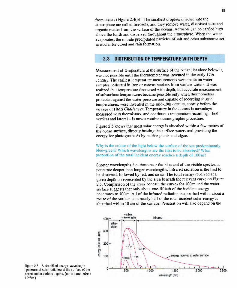
Figure 2.5 shows that most solar energy is absorbed within a few metres of the ocean surface, directly heating the surface waters and providing the energy for photosynthesis by marine plants and algae.

Why is the colour of the Hght lielow the surface of the sea predominantly blue-green? Which wavelengths are the first to be absorbed? What proportion of the total incident energy reaches a depth of 100 m?

Shorter wavelengths, i.e. those near the blue end of the visible spectrum, penetrate deeper than longer wavelengths. Infrared radiation is the first to be absorbed, followed by red, and so on. The total energy received at a given depth is represented by the area beneath the relevant curve on Figure 2.5. Comparison of the areas beneath the curves for 100 m and the water surface suggests that only about one-fiftieth of the incident energy penetrates to 100 m. All of the infrared radiation is absorbed within about a metre of the surface, and nearly half of the total incident solar energy is absorbed within 10 cm of the surface. Penetration will also depend on the

Figure 2.5 A simplified energy-wavelength spectrum of solar radiation at the surface of the ocean and at various depths, (nm = nanometre = 10-9m.)

visible 400 [- wavelengths infrared

500 1 000 1 500

wavelength (nm)

2 000 2 500

from coasts (Figure 2.4(b)). The smallest droplets injected into the atmosphere are called aerosols, and they remove water, dissolved salts and organic matter from the surface of the oceans. Aerosols can be carried high above the Earth and dispersed throughout the atmosphere. When the water evaporates, the minute precipitated particles of salt and other substances act as nuclei for cloud and rain formation.

20

1000

2 000

3 000

4 000

5 000

(a) South

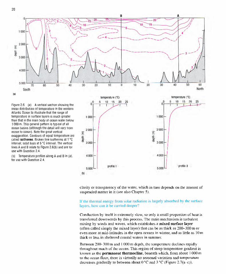
Figure 2.6 (a) A vertical section showing the mean distribution of temperature in the western Atlantic Ocean to illustrate that the range of temperature in surface layers is much greater than that in the main body of ocean water below 1 000 m. This general pattern is typical of all ocean basins (although the detail will vary from ocean to ocean). Note the great vertical exaggeration. Contours of equal temperature are called isotherms. Broken line isotherms at 1 °C interval; solid lines at 5 °C interval. The vertical lines A and B relate to Figure 2.6(b) and are for use with Question 2.4.

(b) Temperature profiles along A and B in (a), for use with Question 2.4.

1000

2 000

dept

h (m

)

3 000

4 000

5 000"-

temperature (°C)

5 10 15 20 T

50 60

North

temperature (X)

0 5 10 15 20 25 0| 1 1 L - J

l O O O h

2 000h

profile I

3 000h

4 0 0 0 h

5 000 L i profile I

(b)

clarity or transparency of the water, which in turn depends on the amount of suspended matter in it (see also Chapter 5).

If the ihermal energy from solar radiation is largely absorbed by the surface layers, how can it be carried deeper?

Conduction by itself is extremely slow, so only a small proportion of heat is transferred downwards by this process. The main mechanism is turbulent mixing by winds and waves, which establishes a mixed surface layer (often called simply the mixed layer) that can be as thick as 200-300 m or even more at mid-latitudes in the open oceans in winter, and as little as 10 m thick or less in sheltered coastal waters in summer.

Between 200-300 m and 1 000 m depth, the temperature declines rapidly throughout much of the ocean. This region of steep temperature gradient is known as the permanent thermocline, beneath which, from about 1 000 m to the ocean floor, there is virtually no seasonal variation and temperature decreases gradually to between about 0 °C and 3 °C (Figure 2.7(a-c)).

21

Important notes Sections and profiles: A vertical section is an imaginary slice through a part of the ocean, to show both vertical and horizontal distribution (commonly represented by contours) of some property (temperature, salinity, density, and so on); e.g. Figure 2.6(a). A vertical profile is a graph showing how some property (temperature, salinity, etc.) varies with depth at a single location in the ocean; e.g. Figure 2.6(b).

Gradients on profiles: A near-vertical part of a temperature profile means that there is little change of temperature with depth (e.g. lower parts of profiles in Figure 2.6(b)). A near-horizontal part of a temperature profile means a large change of temperature with depth (e.g. upper parts of profiles in Figure 2.6(b)). So, when you read or hear of a 'steep temperature gradient' or 'steep thermocline' , that is where the profile is near-horizontal and the rate of change of temperature with depth is greatest. Exactly the same applies to profiles for any other property (salinity, density, etc.).

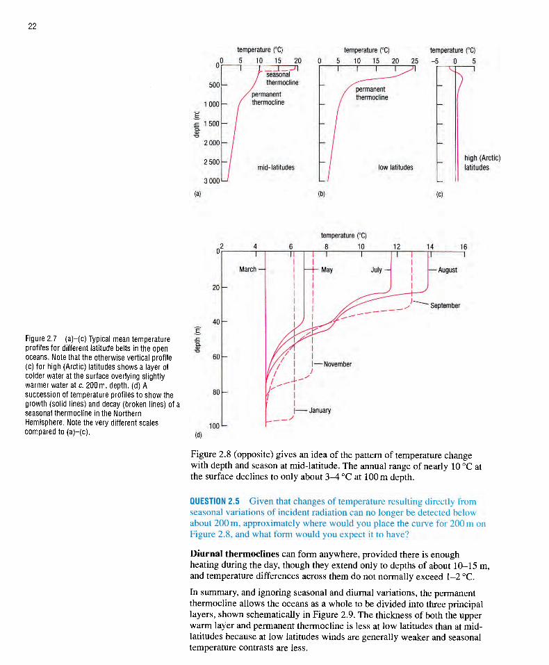
Above the permanent thermocline, the distribution of temperature with depth shows seasonal variations, especially in mid-latitudes. During the winter, when surface temperatures are low and conditions at the surface are rough, the mixed surface layer may extend to the permanent thermocline; i.e. the temperature profile can be effectively vertical through the top 200-300 m or more. In summer, as surface temperatures rise and conditions at the surface are less rough, a seasonal thermocline often develops above the permanent thermocline, as shown in the generalized profile of Figure 2.7(a).

Seasonal thermoclines start to form in spring and reach their maximum development (i.e. with greatest rate of change of temperature with depth or steepest temperature gradients) in the summer. They develop at depths of a few tens of metres, with a thin mixed layer above (Figure 2.7(a)). Winter cooling and strong winds progressively increase the depth of seasonal thermoclines and reduce the temperature gradient along them; eventually the mixed layer reaches its full thickness of 200-300 m (see Figure 2.7(d)). In low latitudes, there is no winter cooling, so the 'seasonal thermocline' becomes 'permanent ' and merges with the permanent thermocline at depths of 100-150 m (Figure 2.7(b)). At high latitudes greater than about 60° there is no permanent thermocline (Figures 2.6 and 2.7(c)), though seasonal thermoclines can still develop in summer.

This narrow range is maintained throughout the deep oceans, both geographically and seasonally, because it is determined by the temperature of cold, dense water that sinks from the polar regions and flows towards the Equator (see Section 4.1).

Q U E S T I O N 2.4 Figure 2.6(a) is a vertical section illustrating the range of temperatures encountered in the oceans, and Figure 2.6(b) shows temperature profiles along lines A and B in Figure 2.6(a).

(a) Match the profiles I and II in Figure 2.6(b) with vertical lines A and B in Figure 2.6(a).

(b) What can you say about the vertical distribution of temperature at high latitudes (above about 60° N and 60° S)?

22

3 000

(a)

temperature (°C)

5 10 15 20 T

mid-latitudes

temperature (°C)

5 10 15 20 T

temperature (°C)

-5 0 5

low latitudes high (Arctic) latitudes

(c)

temperature (°C)

10

Figure 2.7 (a ) - ( c ) Typical mean temperature profiles for different latitude belts in the open oceans. Note that the otherwise vertical profile (c) for high (Arctic) latitudes shows a layer of colder water at the surface overlying slightly warmer water at c. 200 m, depth, (d) A succession of temperature profiles to show the growth (solid lines) and decay (broken lines) of a seasonal thermocline in the Northern Hemisphere. Note the very different scales compared to (a ) - ( c ) .

September

- January

100 L-

(d)

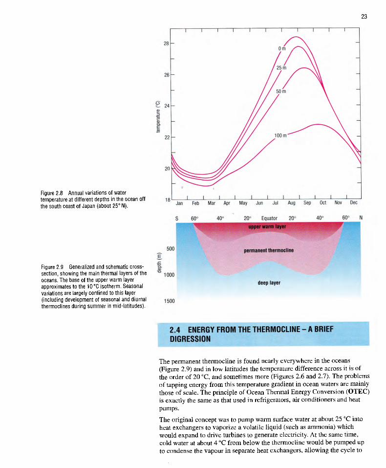
Figure 2.8 (opposite) gives an idea of the pattern of temperature change with depth and season at mid-latitude. The annual range of nearly 10 °C at the surface declines to only about 3 -4 °C at 100 m depth.

Q U E S T I O N 2.5 Given that changes of temperature resulting directly from seasonal variations of incident radiation can no longer be detected below about 200 m, approximately where would you place the curve for 200 m on Figure 2.8, and what form would you expect it to have?

Diurnal thermoclines can form anywhere, provided there is enough heating during the day, though they extend only to depths of about 10-15 m, and temperature differences across them do not normally exceed 1-2 °C.

In summary, and ignoring seasonal and diurnal variations, the permanent thermocline allows the oceans as a whole to be divided into three principal layers, shown schematically in Figure 2.9. The thickness of both the upper warm layer and permanent thermocline is less at low latitudes than at mid-latitudes because at low latitudes winds are generally weaker and seasonal temperature contrasts are less.

(b)

November

March May July - August

23

Figure 2.8 Annual variations of water temperature at different depths in the ocean off the south coast of Japan (about 25° N) .

28 h

26

(Go) 8Jn;B

jadLU9}

181 \ \ \ \ \ \ \ \ 1 \ \ Jan Feb Mar Apr May Jun Jul Aug Sep Oct Nov Dec

S 60° 20° Equator 20°

Figure 2.9 Generalized and schematic cross-section, showing the main thermal layers of the oceans. The base of the upper warm layer approximates to the 10°C isotherm. Seasonal variations are largely confined to this layer (including development of seasonal and diurnal thermoclines during summer in mid-latitudes).

500

1000

1500

permanaiittftermoeSfite

deep layer

2.4 ENERGY FROM THE THERMOCLINE - A BRIEF DIGRESSION

The permanent thermocline is found nearly everywhere in the oceans (Figure 2.9) and in low latitudes the temperature difference across it is of the order of 20 °C, and sometimes more (Figures 2.6 and 2.7). The problems of tapping energy from this temperature gradient in ocean waters are mainly those of scale. The principle of Ocean Thermal Energy Conversion (OTEC) is exactly the same as that used in refrigerators, air conditioners and heat pumps.

The original concept was to pump warm surface water at about 25 °C into heat exchangers to vaporize a volatile liquid (such as ammonia) which would expand to drive turbines to generate electricity. At the same time, cold water at about 4 °C from below the thermocline would be pumped up to condense the vapour in separate heat exchangers, allowing the cycle to

dept

h (m

)

24

Vacuum chamber

Spout evaporator

Discharge

(a)

Direct-contact condenser

Discharge

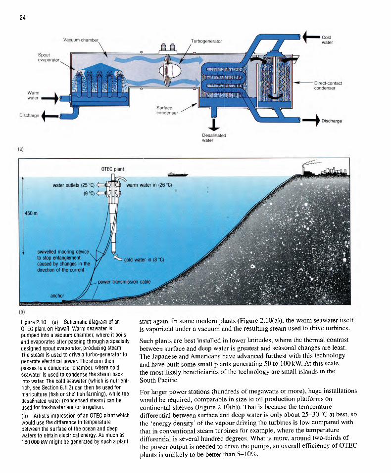
Figure 2.10 (a) Schematic diagram of an OTEC plant on Hawaii. Warm seawater is pumped into a vacuum chamber, where it boils and evaporates after passing through a specially designed spout evaporator, producing steam. The steam is used to drive a turbo-generator to generate electrical power. The steam then passes to a condenser chamber, where cold seawater is used to condense the steam back into water. The cold seawater (which is nutrient-rich, see Section 6.1.2) can then be used for mariculture (fish or shellfish farming), while the desalinated water (condensed steam) can be used for freshwater and/or irrigation, (b) Artist's impression of an OTEC plant which would use the difference in temperature between the surface of the ocean and deep waters to obtain electrical energy. As much as 160 000 kW might be generated by such a plant.

start again. In some modem plants (Figure 2.10(a)), the warm seawater itself is vaporized under a vacuum and the resulting steam used to drive turbines.

Such plants are best installed in lower latitudes, where the thermal contrast between surface and deep water is greatest and seasonal changes are least. The Japanese and Americans have advanced furthest with this technology and have built some small plants generating 50 to lOOkW. At this scale, the most likely beneficiaries of the technology are small islands in the South Pacific.

For larger power stations (hundreds of megawatts or more), huge installations would be required, comparable in size to oil production platforms on continental shelves (Figure 2.10(b)). That is because the temperature differential between surface and deep water is only about 25-30 °C at best, so the 'energy density' of the vapour driving the turbines is low compared with that in conventional steam turbines for example, where the temperature differential is several hundred degrees. What is more, around two-thirds of the power output is needed to drive the pumps, so overall efficiency of OTEC plants is unlikely to be better than 5-10%.

25

2.5 TEMPERATURE DISTRIBUTION AND WATER MOVEMENT

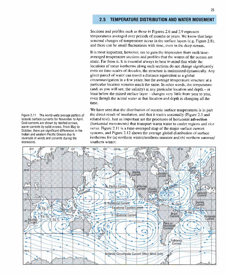
Figure 2.11 The world-wide average pattern of oceanic surface currents for November to April. Cool currents are shown by dashed arrows, warm currents by solid arrows. From May to October, there are significant differences in the Indian and western Pacific Oceans due to reversals of winds and currents during the monsoons.

Sections and profiles such as those in Figures 2.6 and 2.9 represent temperatures averaged over periods of months or years. We know that large seasonal changes of temperature occur in the surface layers (e.g. Figure 2.8), and there can be small fluctuations with time, even in the deep oceans.

It is most important, however, not to gain the impression from such time-averaged temperature sections and profiles that the waters of the oceans are static. Far from it. It is essential always to bear in mind that while the locations of mean isotherms along such sections do not change significantly even on time-scales of decades, the structure is maintained dynamically. Any given parcel of water can travel a distance equivalent to a global circumnavigation in a few years; but the average temperature structure at a particular location remains much the same. In other words, the temperature (and, as you will see, the salinity) at any particular location and depth - at least below the mixed surface layer - changes very little from year to year, even though the actual water at that location and depth is changing all the time.

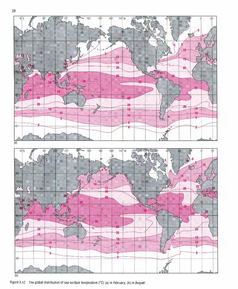
We have seen that the distribution of oceanic surface temperatures is in part the direct result of insolation, and that it varies seasonally (Figure 2.3 and related text). Just as important are the processes of horizontal advection (horizontal movements) that transport warm water to cooler regions and vice versa. Figure 2.11 is a time-averaged map of the major surface current systems, and Figure 2.12 shows the average global distribution of surface isotherms for (a) northern winter/southern summer and (b) northern summer/ southern winter.

26

Figure 2.12 The global distribution of sea-surface temperature (°C) (a) in February, (b) in August.

27

There is a general poleward displacement of isotherms on the western sides of these ocean basins and an equatorwards displacement on the eastern sides (also seen in Figure 2.3). Poleward-flowing currents carry warm water from low to high latitudes - and the effect of the Gulf Stream in carrying relatively warm water across the Atlantic can be clearly seen. Currents flowing towards the Equator (e.g. Canaries Current, Benguela Current) carry cool water from high to low latitudes, resulting in lower average surface temperatures on eastern margins of the ocean basins.

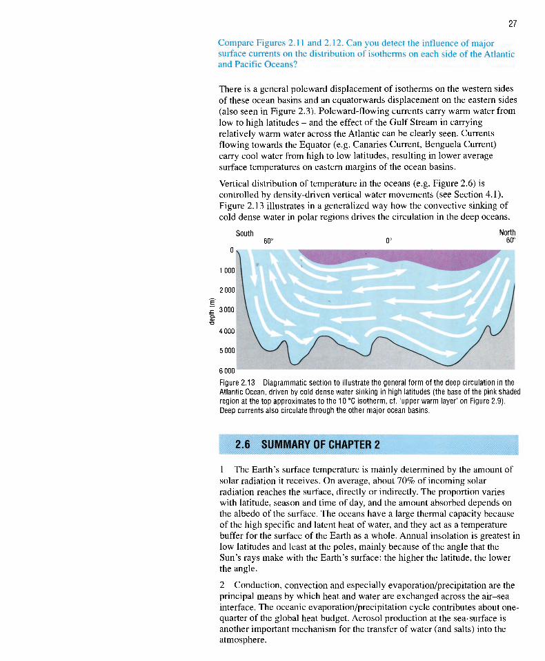
Vertical distribution of temperature in the oceans (e.g. Figure 2.6) is controlled by density-driven vertical water movements (see Section 4.1). Figure 2.13 illustrates in a generalized way how the convective sinking of cold dense water in polar regions drives the circulation in the deep oceans.

South North 60°

6 000

Figure 2.13 Diagrammatic section to illustrate the general form of the deep circulation in the Atlantic Ocean, driven by cold dense water sinking in high latitudes (the base of the pink shaded region at the top approximates to the 10°C isotherm, cf. 'upper warm layer' on Figure 2.9). Deep currents also circulate through the other major ocean basins.

2.6 SUMMARY OF CHAPTER 2

1 The Earth's surface temperature is mainly determined by the amount of solar radiation it receives. On average, about 70% of incoming solar radiation reaches the surface, directly or indirectly. The proportion varies with latitude, season and time of day, and the amount absorbed depends on the albedo of the surface. The oceans have a large thermal capacity because of the high specific and latent heat of water, and they act as a temperature buffer for the surface of the Earth as a whole. Annual insolation is greatest in low latitudes and least at the poles, mainly because of the angle that the Sun's rays make with the Earth's surface: the higher the latitude, the lower the angle.

2 Conduction, convection and especially evaporation/precipitation are the principal means by which heat and water are exchanged across the air-sea interface. The oceanic evaporation/precipitation cycle contributes about one-quarter of the global heat budget. Aerosol production at the sea-surface is another important mechanism for the transfer of water (and salts) into the atmosphere.

Compare Figures 2.11 and 2.12. Can you detect the influence of major surface currents on the distribution of isotherms on each side of the Atlantic and Pacific Oceans?

28

3 Solar radiation penetrates no more than a few hundred metres into the oceans, and most is absorbed within the topmost 10 m. Downward transfer of heat is mainly by mixing, as conduction is very slow (water is a very poor conductor of heat). Mixing by winds, waves and currents produces a mixed surface layer which can be 200-300 m thick or more in winter in mid-latitudes. Below this lies the permanent thermocline, across which temperature declines to about 5 °C, and below which temperature decreases gradually to the bottom (typically between 0 °C and 3 "^C). In mid-latitudes, a seasonal thermocline can develop during summer, above the permanent thermocline. There may also be diurnal thermoclines, at depths of 10-15 m.

4 The temperature difference across the permanent thermocline can be utilized to generate electricity, using the principles upon which the domestic refrigerator is based. The main problem in this application is that of scale.

5 The long-term stability of the distribution of temperature within the ocean means that sections and profiles of average temperature do not change significantly from year to year. This stable thermal structure is maintained by the continuous three-dimensional motion of the global system of surface and deep currents.

Now try the following questions to consolidate your understanding of this Chapter

Q U E S T I O N 2.6 (a) Explain why water at 4 °C can lie overlain by colder

water in a freshwater lake in a gravitationally stable situation. Could such a

situation develop in the oceans?

(b) Explain why a temperature profile from a freshwater lake will not

show temperatures decreasing with depth to values of less than 4 ' 'C .

Q U E S T I O N 2.7 The broad thermal structure of the oceans allows us to recognize three main layers. Name them and summarize their characteristics.