Embed Size (px)
Citation preview
1.
THE NUMERICAL SOLUTION OF HYPERSONIC LAMINAR BOUNDARY
LAYER PROBLEMS
by
Fred Smith, B.Sc.(Eng.)
January, 1973
A thesis submitted for the Degree of Doctor of Philosophy in the Faculty
of Engineering of the University of London.
2.
ABSTRACT
In the present study, the methods of numerical analysis are applied
to two problems which are extremely difficult to handle by an analytical
approach.
The first problem concerns the effects of the ratio of specific
heats and the wall temperature on the separation length of a laminar
boundary layer which is subject to a linearly retarded stream, in the
limit of free stream Mach number tending to infinity. The case of the
linearly retarded stream has been under study for many'years and has
become a yardstick against which techniques and theories have come to
be measured. In the present study, the boundary layer equations are
examined in the limit of Mach number tending to infinity and the
resulting partial differential equations are solved numerically. At
least three significant figure accuracy is achieved.
The second problem is to calculate the flow field over a sharp
nosed, but otherwise arbitrary, body which is subject to a hypersonic
free stream. The flow field is split into viscous and inviscid regions
and the equations in each region are solved separately. Interaction is
effected by defining a boundary layer 'edge' and matching boundary con-
ditions there. The problem is unstable due to the deletion of certain
high order terms and a technique of perturbing the initial values is
used to guide the solution downstream. The program was written so as
to allow human interaction and guidance via a visual display unit, so
that a useful solution can be obtained rapidly.
3.
CONTENTS
ABSTRACT
CONTENTS
ACKNOWLEDGEMENTS
LIST OF ILLUSTRATIONS
NOTATION
PART A
1.0 INTRODUCTION
2.0 THEORY
2.1 The effects of Y and SW on separation length
2.2 The case of Y less than - Region 1.
2.3 The case of y greater than - Region 2.
3.0 NUMERICAL SOLUTION OF THE SCALE EQUATIONS 24
3.1 Solution in Region 1 24
3.2 Solution in Region 2 26
3.3 Numerical scheme 26
4.0 DISCUSSION OF THE RESULTS 28
PART B
32
5.0 INTRODUCTION 33
6.0 THEORY 34
6.1 Terminology 34
6.2 The interaction model
35
Page
2
3
6
10
13
14
16
16
20
21
4.
Page
6.3 Downstream behaviour of the solution 40
6.4 Solution of the viscid region 43
6.5 Solution of the inviscid flow region 55
7.0 COMPUTATION 58
7.1 Introduction 58
7.2 Program description 59
8.0 RESULTS AND DISCUSSION 67
APPENDIX A NUMERICAL SOLUTION OF THE BOUNDARY LAYER EQUATIONS. 77
A 1.0 Outline of the method 77
A 2.0 Development of the method
81
APPENDIX B THE STARTING SOLUTION
83
B 1.0 INTRODUCTION
83
B 2.0 THEORY 83
B 2.1 The inviscid region 83
B 2.2 The boundary layer 85
B 3.0 COMPUTATION 86
APPENDIX C LIST OF ROUTINES USED IN METHOD OF PART B 90
APPENDIX D USE OF THE METHOD OF PART B
98
D 1.0 INTRODUCTION
98
D 2.0 CREATION OF AN INITIAL POINT FROM WHICH TO 99 START CALCULATION
5.
Page
D 3.0 RUNNING THE MAIN PROGRAM 101
D 3.1 Control cards and data 101
D 3.2 List of error codes associated with
104 interaction program
REFERENCES
106
TABLES
FIGURES
PROGRAM LISTINGS
6.
ACKNOWLEDGEMENTS
The author wishes to express his gratitude for the generous
and multifarious help and encouragement given by his supervisor,
Mr. J.L. Stollery, throughout the course of this study. Thanks are
also due to Prof. N.C. Freeman for his help with the analysis
presented in part A of the study and also to Prof. K. Stewartson
for several helpful and illuminating discussions.
The staff of the Imperial College Computer Unit, especially
those involved with computer graphics, musebe mentioned for their
assistance and enthusiasm throughout the final year of this project.
Finally, thanks are due to my silent, quick thinking colleague,
the CDC 6600, who did all the hard work.
7.
LIST OF ILLUSTRATIONS
1. Plot of shear stress factor at the wall, w
against pressure gradient parameter, 0.
116
2 A plot showing the two domains of integration. 117
3 Plot of separation length against wall temperature
parameter for various ratios of specific heats
obtained by the present method.
118
4 Sketch of results from similarity solutions for
adverse pressure gradients.
119
5 Plot of separation length against wall temperature
factor for y = 1.6, 0 = -0.2727.
120
6 Curves of non-dimensional separation length against 121
Mach number for various Sw.
7 Sketch defining the interaction model. 122
8 Sketch defining the mesh point notation. 123
9 Sketch showing the method of determining the path of
the final solution.
124
10 The options display. 125
11 The abort display. 126
12 The epsilon display. 127
13 Key to information display features. 128
Page
8.
Page
14 129 DELSTR display - Plot of s-1-/Fle—s- against (x/L).
15 CFRTRX display - Plot of Cf/F; against (x/L). 130
16 STRTRX display - Plot of St/Res against (x/L). 131
17 SUB S display - Plot of (71;,-)e against (x/L). 132
18 Physical display. 133
19 Flow chart of subroutine TV.
20 Flow chart of program to calculate interactive solution. 146
21 An example of CALCOMP plotter output produced on calcula-
tion of each segment of final solution.
152
22 Flow chart of boundary layer program as used by calculation
described in part A.
153
23 ' Flow chart of boundary layer method in subroutine form as
used in work described in part B
156
24 Plot of the domains of strong and weak interaction and
merged flow.
158
25 Flow over a flat plate: physical plane. 159
26 Pressure distribution on a flat plate. 160
27 Heat transfer to a flat plate. 161
28 Displacement thickness on a flat plate. 162
29 The cubic power law body Y = X3/150. 163
9.
Page
30 Flow over the cubic power law body: physical plane. 164
31 Pressure on the cubic model. 165
32 Heat transfer to the cubic model. 166
33 Displacement thickness on the cubic,model. 167
34 Schlieren photograph of the flow over the cubic model. 168
35 Sketch showing the effects of the starting value of
169
x with a controlling perturbation of 5 significant
figures.
36 The card deck required to run the SETUP job. 170
37 The card deck required to run the creation job. 171
38 The card deck required to run a calculation job. 172
NOTATION
a speed of sound
C scaled viscosity coefficient
Cp specific heat at constant pressure
Cv specific heat at constant volume
e nondim.ensional entropy function (see equation 6.2)
E error bound
G scaled velocity function, u/ u,
h enthalpy
I entropy
k thermal conductivity
L reference length
m Mach number parameter, 'l(y - 1)M!
M Mach number
n normal co-ordinate.
p pressure
Pr Prandtl number
q flow speed, 412 4. v2
heat transfer rate
R universal gas constant
Re Reynolds number
s streamwise co-ordinate
S nondimensionalised total enthalpy function as used in
part A (see equation 2.4)
S nondimensionalised total enthalpy function as used in part B
(see equation 6.15)
T absolute temperature
u streamwise velocity component
10.
1L
v normal velocity component
x free stream direction
y direction normal to free stream
a Mach angle
pressure gradient parameter (see equation 2.11)
ratio of specific heats
6 boundary layer thickness
6* boundary layer displacement thickness
small perturbation
normal co-ordinate in transformed plane
0 direction of flow with respect to free stream direction
viscosity
kinematic viscosity
streamwise direction in transformed plane
p density
a shock angle
T shear stress
viscous interaction parameter, Me3 /(717—
stream function
perturbation (see equation 6.6)
subscripts
e at the effective body
L referred to reference length
M evaluated at the Mth normal mesh point
N evaluated at the Nth
streamwise mesh point
s referred to s co-ordinate
w at the wall
12,
x referred to x co-ordinate
o free stream stagnation condition
00 free stream condition
superscripts
p pth level of iteration
non dimensionalised value.
Note
Any name or group of characters appearing within the text in
the upper case should be regarded as a Fortran variable name or a
computer system command.
13.
PART A
THE EFFECTS OF THE RATIO OF THE SPECIFIC HEATS AND WALL TEMPERATURE
ON THE SEPARATION LENGTH OF A LAMINAR BOUNDARY LAYER IN A LINEARLY
RETARDED STREAM IN THE ASYMPTOTE OF FREE STREAM MACH NUMBER TENDING
TO INFINITY
14.
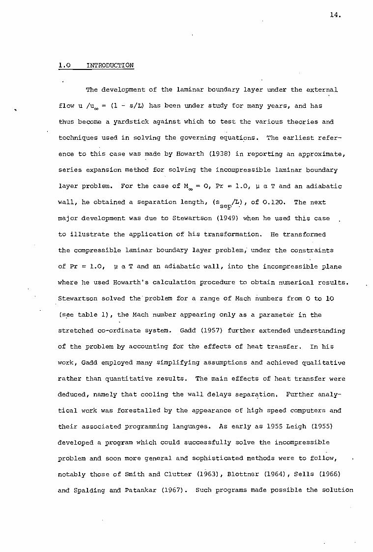
1.0 INTRODUCTION
The development of the laminar boundary layer under the external
flow u /um = (1 - s/L) has been under study for many years, and has
thus become a yardstick against which to test the various theories and
techniques used in solving the governing equations. The earliest refer-
ence to this case was made by Howarth (1938) in reporting an approximate,
series expansion method for solving the incompressible laminar boundary
layer problem. For the case of M. = 0, Pr = 1.0, p a T and an adiabatic
wall, he obtained a separation length, (ssep
/L), of 0.120. The next
major development was due to Stewartson (1949) when he used this case
to illustrate the application of his transformation. He transformed
the compressible laminar boundary layer problem; under the constraints
of Pr = 1.0, p a T and an adiabatic wall, into the incompressible plane
where he used Howarth's calculation procedure to obtain numerical results.
Stewartson solved the'problem for a range of Mach numbers from 0 to 10
(see table 1), the Mach number appearing only as a parameter in the
stretched co-ordinate system. Gadd (1957) further extended understanding
of the problem by accounting for the effects of heat transfer. In his
work, Gadd employed many simplifying assumptions and achieved qualitative
rather than quantitative results. The main effects of heat transfer were
deduced, namely that cooling the wall delays separation. Further analy-
tical work was forestalled by the appearance of high speed computers and
their associated programming languages. As early as 1955 Leigh (1955)
developed a program which could successfully solve the incompressible
problem and soon more general and sophisticated methods were to follow,
notably those of Smith and Clutter (1963), Blottner (1964), Sells (1966)
and Spalding and Patankar (1967). Such programs made possible the solution
15.
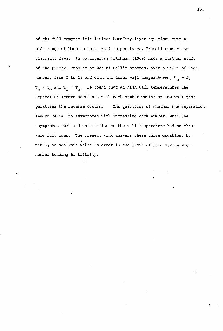
of the full compressible laminar boundary layer equations over a
wide range of mach numbers, wall temperatures, Prandtl numbers and
viscosity laws. In particular, Fitzhugh (1969) made a further study -
of the present problem by use of Sell's program, over a range of Mach
numbers from 0 to 15 and with the three wall temperatures, Tw = 0,
Tw = T and Tw = To. He found that at high wall temperatures the
separation length decreases with Mach number whilst at low wall tem-
peratures the reverse occurs. The questions of whether the separation
length tends to asymptotes with increasing Mach number, what the
asymptotes are and what influence the wall temperature had on them
were left open. The present work answers these three questions by
making an analysis which is exact in the limit of free stream Mach
number tending to infinity.
16.
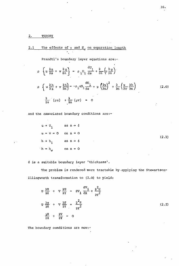
2. THEORY
2.1 The effects of y and Sw on separation length
Prandtl's boundary layer equations are:-
cu au 4. v 31:1 _ u dU1 a ( 3u)_ p
Ds 3n - P 1 1 ds ± n kl-/ @la
dU a h + v a l. -p uU 1 +
r Du)2
+ 3 (p ah)
p { u —
a s an 1 1 ds ' P \ an/ an \ Pr an
a , a -57 {pu} + 7:-.: {pv} = 0 0.
and the associated boundary conditions are:-
u ->- U1 as n-)- cS
u = v = 0 on n = 0
h .4- h1 as n + d
' h = h on n = 0 14
(2.0)
(2.1)
o is a suitable boundary layer 'thickness'.
The problem is rendered more tractable by-applying the Stewartson-
Illingworth transformation to (2.0) to yield:
dV1 + a2U au ,, au = _ sv ___ 2 U — + , ax 7i - 1 dX ay
2 U 0- + v = a2S
ax DY DY2
3U+ DV - _
ax 3Y 0
(2.2)
The boundary conditions are now:-
n
Y = ( p
poo )11 ./ 2 al
a-- o, . aco p d (a) „ r
0
(2.4)
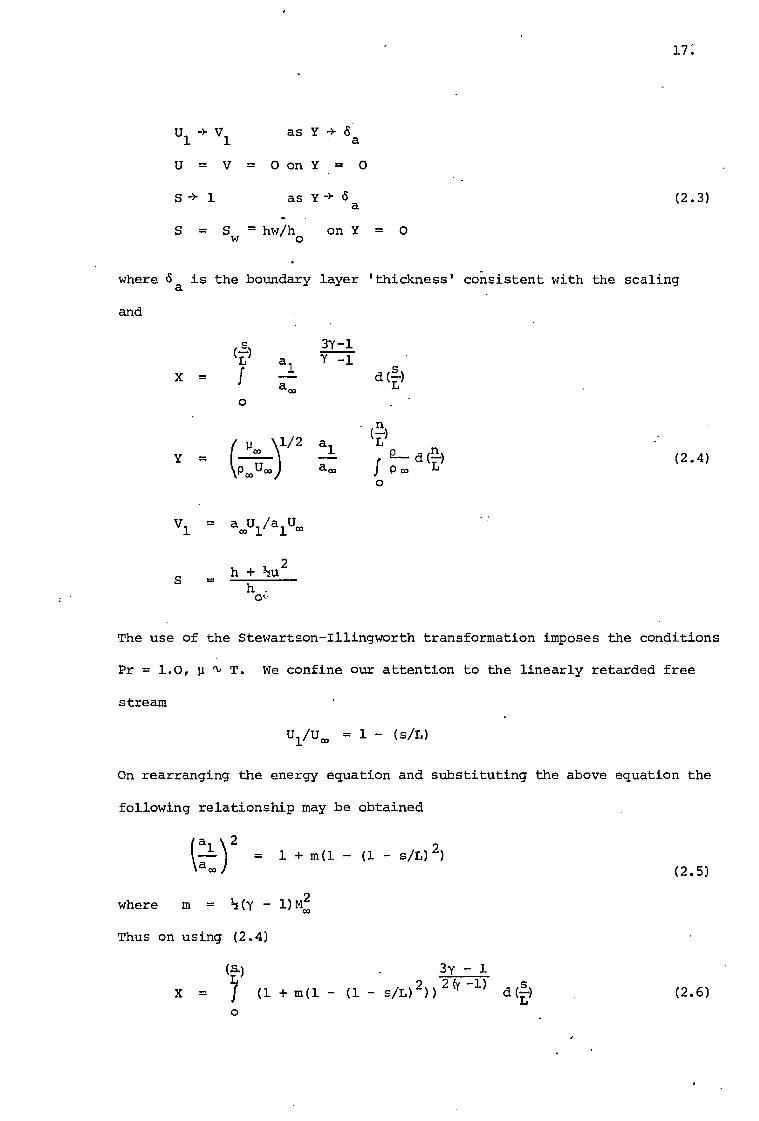
17:
U V as Y 1 1 a
U= V= 0 on Y= 0
5 + 1 as Y+ 5a (2.3)
S = Sw = hw/h on Y = 0
where d a is the boundary layer 'thickness' consistent with the scaling
and
(E) a 1 -1
s 3y-1
a d(2-) X =
co 0
V1 = a.U1/a1Uoo
h + 2
h of
The use of the Stewartson-Illingworth transformation imposes the conditions
Pr = 1.0, 11 ti T. We confine our attention to the linearly retarded free
stream
U1/U = 1 - (s/L)
On rearranging the energy equation and substituting the above equation the
following relationship may be obtained
(aw
a1)2 = 1 m(1 (1 - s/L)2)
where m = 11('( - 1)M!
Thus on using (2.4)
3y - 1
X = (1 + m(1 - (1 - s/L)2))
2(Y -1) dA
(2.5)
(2.6)
18.
and
V1
(1 - s/L) (2.7)
11 + m(1 - (1 - s/L)2)
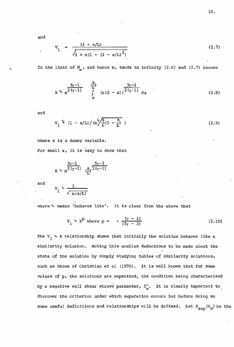
In the limit of M o, and hence m, tends to infinity (2.6) and (2.7) become
3y-1 (1) 3y-1 y f X 1, - m2(-1)
(z(2 - z))2(y-1) dz (2.8) 0
and
V1' (1 — s/L)/(a/L
— s )
(2.9)
where z is a dummy variable.
For small x, it is easy to show that
3y-1 5y-3 m X 'I, m2 (y-1) s() 2 (y-1)
and yl
ti V m(s/L)
where q, means 'behaves like'. It is clear from the above that
V1 q, XP where p = (y - 1) (5y - 3) (2.10)
The V1 X relationship shows that initially the solution behaves like a
similarity solution. Noting this enables deductions to be made about the
state of the solution by simply studying tables of similarity solutions,
such as those of Christian et al (1970). It is well known that for some
values of p, the solutions are separated, the condition being characterised
by a negative wall shear stress parameter, f". It is clearly important to
discover the criterion under which separation occurs but before doing so
1
some useful definitions and relationships will be defined. Let f3sep(Sw)be the

19.
value of $, the pressure gradient parameter, for the incipient separation
condition, f" = 0, and let $min(8) be the smallest value of a for which
similarity solutions exist for each Sw. For example, in figure 1, for
Sw = 0, 0sep and $ are the values of % at the points D and C respect-
ively. From Christians work it is easy to show that
2p p+1 '
so that on using (2.10)
a (y - 1) (2y - 1)
(2.11)
An obvious choice of criterion to test for separation is to compare a and
$Sep
the incipient separation pressure gradient parameter. Inspection of
figure 1, however, shows that this is incorrect for small Sw. For 8w = 0
for example, all the solutions on the arc BD have a a less than 0sep,
whilst
having a positive q. The proper criterion for this case is thus to test
$ against the value of $ at the point C or, in general, to test a against
Omin. It should also be noted that for small Sw, the similarity solutions
for which Brain < $ < asep are doubled valued. For Sw = 0 and such a a,
there is one solution on the arc BC and one on the arc CD.
For large 8w, however, the value of f171 corresponding to %lin is
zero or negative so that a must be larger than 0sep if the solution is to
be attached. The overall criterion is therefore to test $ against amin
forsmallSandagainst, Bsep for large Sw as shown below. The change
over occurs when the two conditions become identical, that is when 13min
has a corresponding f; of zero, the incipient separation condition. Careful
examination of the table of similarity solutions due to Christian et al
shows that this occurs when 5 = 1.0. If the compound criterion is denoted
by $crit(Sw), then we may expect at least one attached solution if
20.
S > a (s ) crit w
where < <
13crit = a min (s w) if 0 - Sw - 1.0
and
°crit = sep(Sw) if 1.0 - Sw
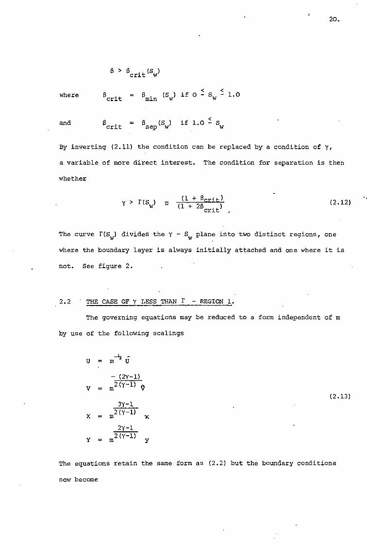
By inverting (2.11) the condition can be replaced by a condition of y,
a variable.of more direct interest. The condition for separation is then
whether
(1 + acrft) y > F(Sw) (1 213 ) crit
(2.12)
The curve F(Sw) divides the y - SW plane into two distinct regions, one
where the boundary layer is always initially attached and one where it is
not. See figure 2.
2.2 ' THE CASE OF y LESS THAN r - REGION 1.
The governing equations may be reduced to a form independent of m
by use of the
u =
V =
following scalings
m 1/2 6
- (2Y-1) m2 (y-1)
(2.13) 3y-1
X = m2 (Y-1)
2y-1
Y = m2 (y-1)
The equations retain the same form as (2.2) but the boundary conditions
now become
xs = I {z(2 - z)}2(y-1) dz (f)s 3Y -1 L
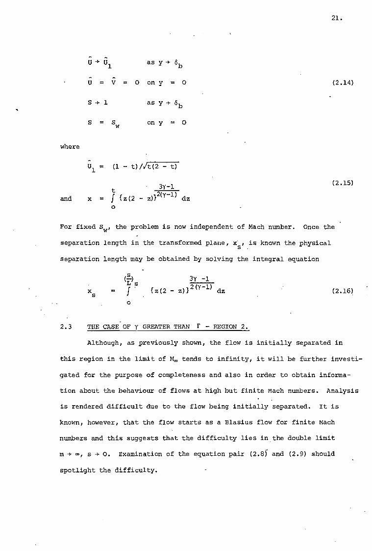
21.
U -> U1
as y db
U= V= 0 on y= 0
(2.14)
S 1 as y 6b
S = Sw on y = 0
where
Ul = (1 - t)/Vt(2 - t)
t 3Y-1
and x = f {z(2 z)}2(1-1) dz 0
(2.15)
For fixed Sw, the problem is now independent of Mach number. Once the
separation length in the transformed plane, xs, is known the physical
separation length may be obtained by solving the integral equation
(2.16)
0
2.3 THE CASE OF y GREATER THAN r - REGION 2.
Although, as previously shown, the flow is initially separated in
this region in the limit of Mm tends to infinity, it will be further investi-
gated for the purpose of completeness and also in order to obtain informa-
tion about the behaviour of flows at high but finite Mach numbers. Analysis
is rendered difficult due to the flow being initially separated. It is
known, however, that the flow starts as a Blasius flow for finite Mach
numbers and this suggests that the difficulty lies in the double limit
m s 4 0. Examination of the equation pair (2.8) and (2.9) should
spotlight the difficulty.
22.
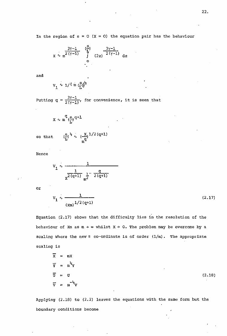
In the region of s = 0 (X = 0) the equation pair has the behaviour
3y-1 (21-) 3y-1 2(y-1) 2 (y-1) X 1, m (2z) dz
0
and
V1 m (10 1
Putting q -- 23(:11), for convenience, it is seen that
q s q+1 X 4, m
so that LS1/2(q+1) %mg,
Hence
V1
1
x2(q+1) 2(q+1) m2
1
or
V1 ft,
1
(Xm)1/2(q+1)
(2.17)
Equation (2.17) shows that the difficulty lies in the resolution of the
behaviour of Xm as m 00 whilst X-} 0. The problem may be overcome by a
scaling where the new S co-ordinate is of order (1/m). The appropriate
scaling is
X = mx
= U (2.18)
V = m-11V
Applying (2.18) to (2.2) leaves the equations with the same form but the
boundary conditions become
23.
(y-l)
U } U1 (1 + (51 - 3)/(y - i)Fe (5y-3) as 7 ÷
U. . V= 0 on Y= 0 (2.19)
S ÷ 1 as 7 + 6c
S + Sw on 7 = 0
where do is a boundary layer thickness consistent with the scaling.
The equations are again Mach number independent and the physical separation
length is obtained from the separation length in the scaled plane, is, by
(s/L) s 1 = ;7(1 + (5y 3)/(y
3)- 2(1-1)/(51-3) (2.20)
3 NUMERICAL SOLUTION OF THE SCALED EQUATIONS
3.1 SOLUTION IN REGION 1
The behaviour of the scaled s co-ordinate and the external velocity
near the origin may be obtained by setting t to a small value in equations
(2.15). It is seen that:-
UI A, 1/)/T
and 5y -3 x `‘' t 2 (y-1)
so that (y-1)
Ul x 5y-3
It is clear that for y greater than unity,U1 is infinite at the origin.
This is unacceptable if the equations are to be solved numerically since
the digital computer stores values as a finite number of binary digits.
The difficulty may be removed, however, by employing a modified form of
the G8rtler transformation.
E = f U1 dx
n + A () = YZJ1/1/2 U1dx (3.1)
= + n )
The variable A() is introduced so that the stream function may be
shifted so as to take a value of zero at the 'edge' of the boundary layer.
This helps to reduce error in the numerical procedure. The equations
obtained on transformation are:-
25.
F nnn
+ (F + n)F nn
+ 0[S - (F + 1)2] = n[F (Fn + 1) - FF j
S + (F + n)S = 2g[s (Fn + 1) - s
nF]
where 20, x
(C) = ix r 1 dx 2 J
Ul
(3.2)
The boundary conditions are now
F = 0 as n dd
F = _n = A and F = -1 on y = 0 (3.3)
S 1. as n dd
S Sw on y =0
where dd is the boundary layer thickness in the transformed plane.
Since A is a function of it.is clear that the region of integration
is of variable width and so we must employ a further transformation to
facilitate computation. The transformation described by (3.4) puts the
< region of integration into the unit semi-infinite strip 0 < - t - 1, x - 0
= g
= + A)/(6d + A) .2 (n + D(E) 6,i)/D( )
• = F (3.4) • K = S - 1
The equations of motion are now
D-
D2
Sd = G {2x (-2-c (1 - - 4)) - c c ] - [49 - 1 + ]1 D
+ 2X G- (G + 1) - 13[K - G - G(G + 1)]
D-d K = K [D21. (1 - - 4)) - 4)5i ] - [4) + - 1 + }
+ 2cc (G + 1)Kil
(3.5)
26.
where G =
The boundary conditions are
= 0, G = 0 on C "= 1
= 1 - dca/D, G = -1 on = 0 (3.6)
K = 0 on = 1
K = (Sw - 1) on C = 0
The equation 4) = 1 - d/D enables D to be calculated once 4)w is known,
and thus the set of equations is complete.
3.2 SOLUTION IN REGION 2
In this region there is no difficulty with the U1 - X relationship,
as shown by the first of (2.19), and a similarity transformation is appro-
priate. We write
=
n + A (E ) = 1/2 (rJ15)1/7
(3.7)
= (ri13C)1/2(F + n)
Application of (3.7) and then of (3.4) results in equations and boundary
conditions almost identical to (3.5) and (3.6).
3.3 NUMERICAL SCHEME
The problemtas described by equations (3.5) ,and (3.6),requires the
solution of a two point boundary value problem consisting of two linked
second order partial differential equations, one of which is nonlinear.
In order to remove the difficulties associated with the coupling and
non-linearities, an iteration scheme is introduced similar to that des-
cribed in part B. Details of the differencing scheme and solution algorithm
are given in appendix A. The program was written in Fortran and calculations
27.
were run on the University of London's CDC 6600 machine, a typical
run requiring 23000 words of central memory and 80 seconds central
processor time. The integral equation (2.16) for (S/L)s was solved
numerically by expanding the integrand as a polynomial in 2z. This
was then integrated term by term and the resulting equation was solved
to obtain the root corresponding to (s/L)s by use of a Newton-Raphson
iteration procedure. The procedure was programmed to automatically
include sufficient terms in the expansion to give six figure accuracy.
28.
4.0 DISCUSSION OF THE RESULTS
The results of the calculations are values of separation length
for various values of y and Sw and these are presented graphically in
figure 3. A remark about the usage of the term 'separation length'
as used to describe the results presented herein is appropriate. The
values were obtained by finding the co-ordinate of the point at which
the shear stress at the wall was zero, by means of extrapolating the
shear stress parameter against streamwise co-ordinate curve. A precise
definition of the separation point is given by Stewartson (1964) who
defines it to be the point where the boundary layer equations develop a
singularity and break down and where, physically, the boundary layer
abruptly thickens and leaves the body. He further points out that the
point of zero skin friction and singularity are not co-incident for the
non-adiabatic wall case - the singularity lies slightly upstream of the
point of zero skin friction if the wall is cooled and vice versa if the
wall is heated.
Buckmaster (1970) further examines the compressible boundary layer
equations in the region of the separation point for the case of a cooled
wall and he finds that extra terms must be added to Stewartson's solution
in order to free it from inconsistencies. As a result of this he finds
that, close to separation, the skin friction coefficient varies as sIlln(s)
rather than s1/2 where s is measured from the separation point in the up-
stream direction. A discussion of the mathematical nature of the boundary
layer equations near the separation point is given in a review paper by
Brown and Stewartson (1969).
The present use of the term 'separation length' is, therefore, not
correct in the sense of Stewartson, but is used as a convenient shorthand
for 'the length to the point of zero shear stress at the wall'.
29.
The solid portions of the curves in figure 3 were obtained from
computation and the points for which (s/L)sep = 0 were obtained by com-
piling a table of S for which f" is zero against Sw from similarity .
solutions. The required Sw is then obtained by interpolating in the
table using the appropriate 0 computed from equation (2.11).
The dotted portions of the curves are approximate but may be
justified by the following argument. It was previously shown that, for
some combinations of S and Sw, similarity solutions provide two sets of
initial values from which the subsequent flow may be calculated. Now
since the external velocity profile is identical for both cases (y is the
same in each case) two values of separation length are to be expected,
the smaller corresponding to the initial data with the lower f". A check
on the present calculations at the origin showed that they started from
initial values on arcs such as the one labelled AC in figure 1 for the
case Sw = 0. The present numerical scheme was unable to compute solutions
from initial values on arcs such as CD.
In order, to confirm the possibility of calculating solutions from
initial values with s less than 8 especially with f3 close to13min, as selp
predicted in theory, a set of detailed calculations were performed. For
ease of computation, a scheme of varying Sw whilst holding 'y at a constant
value of 1.6 was employed. The scheme is shown graphically in figure 4.
The previous theory predicts the following results.- Fixing y fixes a
and, as shown in figure 4, increasing Sw shifts the f" against S curve
to the right and slightly downwards. For Sw = 0 the initial value lies on
the arc AB, that is 13. is larger than the corresponding a sep .. An attached
flow is to be expected. As Sw is increased the shifting of the fy::7 -
curve increases the corresponding (3sep until 0 is less than sep If the pre-
sent theory is correct, the solution should still be attached and thus have
30.
a non-zero separation length, until increasing Sw so shifts the curve
that a is equal to 0min. Further increase of Sw should result in a
being to the left of the f4J - S curve resulting in a non-existent
solution and consequent numerical breakdown. The increase of Sw
throughout the process results'in a reduced initial value of f; and,
since the external flow is invariant, a reduced separation length.
Since the last calculable flow has a 0 equal to 0min and a positive
f", the separation length should be non-zero at breakdown. This is
exactly the behaviour obtained by calculation as shown in figure 5.
It should be noted that solutions are obtainable for Sw less than
0.4566 and that the separation length has a finite value of 8.82 x 10⁻³
just before breakdown. A suitable check to assure that 0 is very close
to 0 mln
is to interpolate in a table of amin against Sw, taken from
similarity solutions, for Sw =. 0.4566, the value at which breakdown
occurred, to obtain 0Inin and then use the inverse of (2.11) to obtain y.
On so doing an y of 1.601 is obtained agreeing very closely with the
input value of 1.6. By interpolating in a table of asep against Sw for
a = -0.2727, which corresponds to y = 1.6, the value of Sw corresponding
to the incipient separation condition was found to be 0.456. In accordance
with the present theory, attached solutions were found for Sw smaller than
this.
'In order to check the accuracy of the present results, a series of
numerical solutions of the laminar boundary layer equations under the
present conditions, for a range of Sw and Mme, were obtained by running
the Spalding and Patankar program. The results are shown in figure 6.
The present results, which are valid for infinite M, agree very closely
with the asymptotes derived from the solution at finite Mach number. The
maximum discrepancy is of the order of 0.2%.

31.
Figure 6 shows again that cooling the wall tends to delay the
separation of a laminar boundary layer. The Mach number limitation
effect is also evident, although not in the usual sense because in the
present problem it is the external flow that is invariant and not the
geometry of the wall. Fitzhugh (1969) gives the family of bodies which
are required to produce a linearly retarded stream for a series of free
stream Mach numbers from 2 to 10.
32.
PART B
THE NUMERICAL CALCULATION OF THE DISPLACEMENT INTERACTION OF A
HYPERSONIC LAMINAR BOUNDARY LAYER ON A SHARP NOSED BUT OTHERWISE
ARBITRARY BODY
33.
PART B
5.0 INTRODUCTION
The boundary layer equations and the equations of supersonic
inviscid flow are respectively parabolic and hyperbolic in nature so
that, given a set of initial data and suitable boundary conditions,
their mathematical nature allows the calculation of downstream solutions
by a step by step method. The required boundary conditions are a
description of the external flow in the case of the boundary layer
equations and the body geometry in the case of the inviscid equations.
Clearly the results of one set of calculations provide the input to the
other so that, by interactively substituting for the boundary conditions
of one set of equations from the results of the other, it is reasonable
to assume that a full solution of the flow field, including boundary
layer displacement effects, may be calculated. Such a course of calcula-
tion, requiring only a knOwledge of free stream parameters and model geo-
metry, has been undertaken. The model is not entirely self-contained
inasmuch as it needs results from strong interaction theory in order to
provide a set of initial conditions from which to commence calculation.
A small number of test cases have been calculated which are directly
comparable with experimental data obtained either from the Imperial
College gun tunnel or from the literature.
34.
6 THEORY
6.1 TERMINOLOGY
In an attempt to keep the description of the method Concisela
small number of special terms are defined below. The method employs a
marching technique - that is the solution at a downstream station is
computed from a known solution at an upstream station and the boundary
conditions. The solution at each station consists of values specifying
profiles of the transformed velocity, total enthalpy, stream function and
viscosity plus various other parameters, such as the velocity at the edge
of the boundary layer and its derivative in the stream-wise direction,
such as are required to complete the specification of the flow. The
solution which is currently being calculated is called the 'new profile'
and the solution at the last calculated station is called the 'history
profile' since the latter relates the previous development of the flow
to the calculations at the new station. It will be shown that, as calcu-
lation proceeds downstream, it is prone to divergence from the true
solution. Several such diverging calculations are made in order to
locate the path of the true solution and these are accordingly called
'trial runs'. The portion of the true solution obtained as a result of
such trials is called the 'final solution'. The body of data from which
each trial run is started (i.e. the first set of history profiles) is
called the 'initial point'. The physical body plus the deflection
effects due to the boundary layer is known as the 'effective body'.
Each separate submission of the program and data to the computer
is known as a 'job' in order to avoid confusion with the term 'run'.
35.
6.2 THE INTERACTION MODEL
In the classical manner, the flow field is divided into two regions,
one dominated by viscous effects and described by Prandtl's boundary layer
equations and the other essentially inviscid and described by Euler's
equations. The exact boundary layer equations are solved by means of a
modified version of Sell's finite difference program and the inviscid
flow is approximated by the application of Prandtl-Meyer theory.
Due to the complexity of the governing equations and the methods
of solution, any hope of a simultaneous solution of both regions must be
abandoned in favour of an iterative scheme in which each region is solved
alternately, until the results of calculations in each region match at
the effective body.
Consider figure 7 which shows the interaction model and defines the
co-ordinate system used in the present method. Although the boundary layer
equations are often written in terms of the independent variables x and y,
the frame of reference is not Cartesian but one in which the co-ordinates
lie parallel and normal to the local body slope respectively. In order to
emphasize this and avoid confusion, the boundary layer equations are written
here in terms of the independent variables s and n.
The effective body, that is the curve which separates the viscous
and inviscid flow regions, is simply taken to be the physical body plus
the boundary layer displacement thickness. Since the model treats the
effective body as a streamline, the modifying effects of boundary layer
entrainment on the flow angle and total pressure there are precluded. The
effective body is defined by the equation pair
xe- = xw - 6 sin 0
w (6.la)
ye- = yw (x w) 6 cos Qw
36.
Where 6 is the local wall slope (el = tan-1 dT/d7i) and the barred
notation denotes nondimensionalisation with respect to L, the'body
reference length. If the boundary layer and inviscid flow equations are
matched at the effective body, it is clear that the solution will include
the displacement interaction effects.
Taking the effective body to be a streamline is a major assumption
and is therefore worthy of some examination. Consider the case of the flow
over a flat plate for simplicity. By integrating the equation of continuity,
it can be shown that
p v e d f ds
pu do + p ue e ds
0
where S is a measure of the boundary layer thickness defined by a require-
ment such as
u/ue = 0.999 when n =
so now
ve = = 1 d pu
peue
cg fPeue f (1 peue dn - p
eue0 : e u
e
or, on using the definition of displacement thickness
e1 d
Peue Cr; fPeue(6* ds 6)} - c16
which becomes, on rearrangement
ee
d(5* (0 S*)*) 1—(1n(peue)) =
ds ds (6.1b)
The assumption made in writing (6.1a) is that the second term on the right
hand side of the equation above is negligible due to (0 - 0*) being very
small. The conditions under which this is valid may be found by making a
simplified analysis of the flow over an insulated flat plate when the gas
37.
is calorically perfect and has a unit Prandtl number. Under these
conditions, Crocco's integration of the energy equation gives
Pm = 1 + m(1 - (u/u03)2) m = (Y 1) m2
A 2 co
Assuming a linear velocity profile within the boundary layer, it is easy
to show that
1 = f {1 -2-1-1-}dn where n = y/6
p.u.
1 f a 0 1 4. mu - n2i
= ln(1 + (y 2) Mme)
(y (y - 1)mm2
The assumption is valid provided the Mach number is large. If the
problem involves a curved plate, the condition should be interpreted as
a requirement that Me is large. This is reasonable for problems involving
hypersonic flows except in the immediate vicinity of the leading edge
where, according to strong interaction theory, the flow is greatly
retarded. The breakdown of the assumption in this region may be
physically interpreted as being due to appreciable entrainment into the
boundary layer. Consequently it is difficult to determine where the
streamline which ultimately forms the effective body crosses the leading
edge shock and so we are forced to use the approximation given in appendix B
to determine the entropy at the effective body.
There are many possible algorithms which would allow the viscid and
inviscid regions to be matched together, but the one described below was
selected because it did not require numerical differentiation and was
therefore less prone to error. Suppose that the calculations are marching
in steps in s, the full history profiles are known and that the nondimension-
38.
alised s derivative of the velocity at the effective body,( q—) , is s e
the free parameter in the iteration procedure for the solution at the
new station. Reference to §6.4 shows that the boundary layer method
requires a knowledge of s, qe
(ci--) e and ee in order to provide a s
solution. The variable ee is a measure of the entropy at the effective
body and is defined by the equation
Ie - Io (6.2) ee =
Since the effective body is taken to be a streamline, the entropy Is is a
constant and is therefore deduced directly from the history profiles.
The remaining unknown, qe, may be obtained by quadrature from (q—s e)P and N
the history profiles, so that at the pt
•h level of iteration
(cle)NP = (cle)N-1 1/2(sN - sN-1)((ci"S-eN + (ci;
)+ 00((; N-1)2) -N-1
(6.3)
The subscript shows at which streamwise station the variable is evaluated,
the convention being defined in figure 8. Solving the boundary - layer
equations produces a value for (6* -- ti/Res) so that the non-dimensionaLdis-s
placement thickness may be obtained by using
= (-s-6* /Res ) (6.4)
The values xw and y
w are easily calculated from s, the non-dimensional
length along the wall, since the physical body shape is given as an input,
and thus the effective body ordinate obtained by viscous considerations,
(ye)vise, may be calculated by equations (6.1a).
Reference to §6.5 shows that, since xe, qe and ee are known, the
inviscid region may be solved to yield the effective body ordinate obtained
by inviscid considerations, (y ).
P . An absolute error term, cP, for the e inv
th . p iteration may now be defined by
39.
P P — P = (ye)visc - (Ye)inv (6.5)
thus closing the iteration loop. Application of the method of false
positions to the system of equations will systematically reduce the error
to a desired level once two starting pairs of (q-s)e and e are provided.
In practice a good pair of starting guesses for (q-s)e was found to be
- 1 t
(c1;) e = “IT'extrap a)
(6.6) — 2 q;) e = s extrap x (1.0 w) b)
where w is a small perturbing value. The value of (qextrap was obtained
by linear extrapolation in regions of small variation in the s direction,
whilst substitution of the value (q-s )N-1 was found better in regions of e
large variation. The method has been programmed to select the relevant
option automatically., The method of false positions gives an improved
estimate of (q-s)e according to equation
p p-1 - p-1 p I - p+1 (q-V e - (crs-)e e
e p-1 p )
(6.7)
Because of discretisation and rounding, all the numerical processes men-
tioned above contain small errors. Clearly an overall process cannot have
a finer resolution than its components, so to attempt to reduce 6 to zero
would be a waste of effort. Instead a solution is accepted if 6 falls
within the error bound
lel 5 E main (6.8)
where Emain is a small preset positive value. The choice of Emain
is a
compromise between good resolution (small Emain) and the requirement that
each subcomponent should be more accurate than the main iteration (large
Emain), since in practice exact matching of errors is impossible.
40.
Once an acceptable solution is obtained at the new station, the
calculations are stepped forward by simply reclassifying the new profiles
as history profiles, incrementing the s co--ordinate and looping back to
restart the whole procedure.
6.3 DOWNSTREAM BEHAVIOUR OF THE SOLUTION
Since the viscous region of the flow field is approximated by the
boundary layer equations, unsteady and high order s derivative terms are
not present in the model. Physically,this results in the absence of any
direct upstream signalling through the subsonic portion of the boundary
layer. This is demonstrated numerically if it is remembered that the
boundary layer is calculated by a marching procedure whereby a solution
is obtained solely on the basis of a given upstream solution. If upstream
signalling were to be admitted, the whole flow field would have to be
calculated simultaneously so that the effects of each part of the flow
field could be felt throughout. This lack of direct upstream signalling
has a major repercussion on the calculations, namely that the solution
will be prone to divergence arising from the small perturbations due to
rounding, discretisation etc. Qualitatively, the mechanism producing
divergence is as follows. Since the new parameters are calculated using
the history parameters, they will be perturbed from the true solution not
only by the numerical error at the new station but also by the error passed
on from the history parameters, which were themselves produced by a numerical
procedure. Further, the history parameters were already perturbed by errors
arising in the calculation of their predecessor and so on upstream. Garvine
(1968) and Georgeff (1972a) have shown that the problem as posed here is
not stable and so the errors produced at each step tend to be cumulative
producing an 'avalanche effect'. The behaviour of the divergence is clearly
41.
very complex and depends both on the numerical method employed and on
the local values of the variables. Whether the divergence is in a
retarded or accelerated sense depends on the net sign of the perturbing
error and is not calculable in advance. If upstream signalling had been
permitted by the inclusion of elliptic terms in the equations, divergence
due to numerical error would have been inhibited since the flow could
sense and therefore conform to the non-divergent downstream boundary
conditions. Mathematically the problem would have been closely related
to that of Robbins which is both well posed and understood theoretically.
Aerodynamically, the problem would have been to solve the Navier-Stokes
equations which, although more sound in principle than the present method,
has practical difficulties. It has been found that,at flight Reynolds1
numbers,an extremely small computational mesh must be used if error is
not to destroy the solution. Such a requirement makes impossible demands
on current computer space and time. See von Karman Inst. (1972).
. A simple and most effective way of controlling the divergence of
solution is to introduce a small, artificial controlling perturbation to
the initial point. In the present method it is possible to perturb any
combination of five parameters as shown below
(a)PERT = (a)IP x (1 + c1)
e)PERT = (8e )IP (1 + 62)
(cle)PERT = (qe)Ip x (1 + c3)
(ee)PERT = (e
e)11,-. x (1 + 64)
(qs )PERT = (qs )IP x (1 + 65) e e
(6.9)
where the subscript PERT denotes the perturbed value at the initial point
used in subsequent calculations and the subscript IP denotes the existing
value at the initial point. In practice it is found that the values of
42.
N may range between +5 x 10
-3 and -5 x 10
-3. By such adjustments
it is possible for the controlling perturbations to nullify the inter-
nally generated errors, so as to produce a solution which is stable over
a small region. Any hope of producing a fully stable solution by such
an adjustment should be abandoned, since the perturbing errors are pro-
duced spontaneously at every stage of calculation and are very probably
non-linearly dependent on the history of the calculation. The adjustment
of a few parameters could not overcome such effects. A more practical
approach is to generate a pair of trial solutions, one accelerated and
one retarded, which exhibit a degree of stability, as shown in figure 9.
An acceptable final solution may then be calculated from a knowledge of
the pressure gradients under which such trial solutions developed.
In the present method, trial solutions are generated by variation
of the control perturbations until a reasonably stable solution of each
type is produced, whereupon the values of Cf 117s s- and (q--)
e obtained at
each station are stored within the computer. A segment of final solution
is then obtained by recalculating the flow using the average value of
s e , up to the station where the corresponding values of Cf/Fic differ
by more than a preset error bound. See figure 9. A typical error bound
is 0.1 to 0.5 percent of the mean value of Cf/ii-e7; - such an error level
should ensure that the final solution will not differ from the true solution
by a factor greater than the error involved in the numerical solution of the
boundary layer equations. The process of obtaining a new segment of the
final solution results in the creation of a new initial point from the
solution at the last calculated station. Calculation is therefore able to
step progressively downstream by a simple repetition of the whole process
but starting from the last calculated initial point. In order to facilitate
this, the program was written to automatically replace the old initial point
43.
by the new one on sensing that a further segment of final solution had
been calculated.
Rather than altering a few variables out of context, it is
better to adjust the initialpoint by locally linearising the equations,
so that the whole solution might be consistently perturbed. Due to the
complexity of the present computational approach, this was impossible.
However, any gross error in the solution, which would be detected by
discontinuities where segments of final solution join, was not found and
so the simple method of perturbation is valid within the general limits
of accuracy.
A rigorous analysis of the error involved in calculating the solution
segment by segment is not possible due to the complexity of both the
partial differential equations and the numerical analysis. The same is
true of any method of this type (for example that of Klineberg (1968))
but cautious choice of error bounds has been shown to lead to results which
agree well with experiment and, on that basis alone, the technique is used
with some confidence.
6.4 SOLUTION OF THE VISCID REGION
The viscid region is calculated by solving the boundary layer
equations numerically. The gas is assumed to be calorically perfect, have
a linear viscosity-temperature relationship and have a constant Prandtl
number of 0.72. The equations of motion are:-
auDu + a( \ Pu as PI/ an ds an VI an )
2 an ah au a 1 ah p u + pv u + as an ds an an Pr an )
a a as
{oi} 4- 71 {pv} . 0
(6.10)
0 p 0 0
p S
= s
n + A (s)
(6.12)
n qe 1/2 r
j p dn
44.
Following Sells (1966) we define the following non-dimensional variables
s - = s/L n = Re 1/2 n
1/2 u - = u/u = Re v
(6:11)
= P/P P = P/P. co p= Po
p L
U2
17. = h/U:
where Re
Pc„
Scaling (6.10) by use of (6.11) leaves the equations with the same form
as (6.10) but now all quantities are of order unity. In order to remove
most of the effects of density variation, a modified Dorodnitsyn trans-
formation is applied to the equations. The transformation is defined by
=p sq ) ( c) n) 0 o e
where A is a suitable function of Tto shift the origin of n so that the
transformed stream function, 0, tends to zero at the outer 'edge' of the
boundary layer. This technique, first introduced by Smith and Clutter (1963),
is useful in controlling numerical error as shown in the example below.
E
dq
Consider the term - 1/2(1 + n)0 nn
in equation (6.13a). If the qe dE
origin had not been shifted, the stream function, 4, would have rapidly
and unboundedly increased with 71, especially in the hypersonic case due
to the dramatic increase in density as the cool external flow is approached.
The term (4 + n) would then act as a large multiplier on the error caused
by discretising 0 nn
. Near the wall, 0 would be small and would therefore
45.
diminish the effects of the term cb . Clearly this leads to an nn
imbalance of effects and is therefore a source of error. It is easy
to show by similar arguments that shifting the origin solves the problem.
On applying (6.12) to the scaled set (6.10) we obtain
he p e @ E dqe H
o dq 2 (Onn) = -1/2(1 + (4) + n);5 1,1 + + 240n- S)
0 0 e e
[4,n (fin + 1) - inn a) (6.13)
2 (le 2 A - E dqe
he p c a -C r- --- — is + (Pr - 1)7—
Ho(4) n + 24) } = -1/2 (1
qe) (4) + n p @II Pr Dn 0 0
E (fin + 1) - cpE n ] b)
•
where C is a scaled viscosity defined by
— C-- -- at fixed S-- p H
o Ho p (6.14) c)
For a linear variation of viscosity with temperature, which is
assumed throughout thepresent work, C = 1.0. The variable is is defined
by
(6.15) H
O
Inspection of (6.13) shows that four parameters which rely on a knowledge
of the external flow are required. These are
t 1 Ti 1/(Y-1) P = exp (e) h Co
46.
F'
E' dq
e = d
(le
= he p e
H •p - o o
a)
b)
G' = 2 di
e 7.1 c)
(6.16)
—2 — H' = q
e/Ho d)
These may be calculated from, q e , (a..)e and ee by use of the steady flow
energy equation, which in scaled variables is
+ q2/2 = Ho = 17.0 +
(6.17)
and the second law of thermodynamics which, for a calorically perfect gas,
gives
e = y In - (y - 1) In (12--) h.
(6.18)
If it is assumed that air is a perfect gas, the Scaled equation of state is
(6.19)
Combining equations (6.18) and (6.19) gives
(6.20)
on, using the definition p = p/p. to set Fp, to unity. The scaled enthalpy is
obtained directly from (6.17) once the stagnation enthalpy, Ho, is evaluated.
H = + a - U2 00 (y - 1)14
2.
h 1
1 117,2 TRY-1)
Ho F' (exp(ee))1/(y-1) H 0
a)
(6.22)
47.
(6.21)
It may now be shown that
dq G' _ 1721 b)
o
on noting that, since the process co 4- 0 is isentropic,
I - I exp(e0) = exp c (, oca )
= 1.0
The boundary conditions on (6.10) are
u = 0 a)
= 0 on n = 0
b)
h = hw c)
u = qe
d) (6.23)
at n = 6(x) H = Ho e)
where 6(x) is the outer 'edge' of the boundaiy layer. In the new co-ordinate
system, the wall, n = 0, is described by the equation
n = - p(x) (6.24)
Using the definition of the stream function i, namely
p = , ay
= - aW p v ax

48.
it may be shown that, on using (6.12)
u = qe + 1)
(6.25)
By reference to equations (6.12), (6.15), (6.24) and (6.25) it may
be further shown that the boundary conditions (6.23) transform into the
set.
n = - 1
= A (E on n = -A (E)
a)
b)
c)
d)
e)
= Sw f Tw/T0
(6.26)
= 0 fl
= 0 / on n = ni
where n, a constant, defines the outer edge of•the boundary layer in the
transformed plane. Due to the introduction of the origin shift, A, a
condition on 4 may be imposed at the outer edge of the boundary layer.
Thus we set
= 0 . at n = ni (6.26f)
and so close the system of equations, (6.26b) being used to evaluate A.
Equation sets (6.13) and (6.26) are still not amenable to numerical
solution due to four main difficulties, namely a) the momentum equation
contains a third order derivative in n b) it is nonlinear in 4), c) the
momentum and energy equations are coupled and d) the lower bound of inte-
gration in the n direction is variable (see equation 6.24).
The first point, although easy to handle in principle, causes trouble
at a practical level. It will be shown in appendix A that the numerical
scheme reduces each differential equation to a matrix equation
=
49.
where A and B are known and X contains either the desired velocity or
stagnation enthalpy profile. For a second order equation, it turns out
that A has a particularly simple structure - all its elements are zero
except for the three leading diagonals, which results in it being straight-
forward to invert. If the differential equation is of higher order, however,
A contains more non-zero elements and the work of inversion is greatly
increased. The problem is overcome by the simple device of introducing a
variable, G say, where
(6.27)
so that the momentum equation becomes second order in G. The value of (I)
may then be obtained by a quadrature of G. Clearly this forces the intro-
duction of an iteration scheme since both G and (1) appear in the same
equation but the latter may not be obtained until the former is known.
The introduction of iteration also solves b) and c). Any non-
linear terms may now be linearised by simply evaluating one element at
the pth level of iteration and the others at the (p - 1)th level. For
example, (G2 + -2G - e) is linearised to GP(G(P-1) 2) - S. The momentum
and energy equations are uncoupled by solving them serially in an itera-
tive fashion. For example, all the terms involving g may now be evaluated
at the (p - 1)th level during the pth level solution of the momentum
equation for G. In order to accelerate convergence, the latest informa-
tion is always used so that, in the pth level solution for g, the previously
obtained pth level values of G and cp should be used. The introduction of
iteration and the variable G result in equations 6.13 being written as
50.
E E[ (GP-1 + 1) GP - A (P-1)r1P-1 G'[ (GP-1 + 1) GP + GP-1 - -SP-1] -
11(1 + E l ) (GP-1 +-)GP. = F' 3.3r1 [CP-1 q ]
a) (6.28)
[(GP + 1)-SP - -SP1 -. 11(1 EI )(gy 13 + n)sP = E -
1 Pr a
F' 3n n {CP1[113 + - 1)H'GP (GP + 1)11 , b)
n n
where CPI is evaluated from .P, GP and SP-1.
The fourth difficulty, the use of a region of integration whose
width is not constant, raises some practical problems in the placing of
mesh points and also in the difference representation of the E derivatives.
The solution of such problems lies in transforming the region of integration
into a unit semi-infinite strip by use of
s 0 a)
n + A - n + D - n
b) (6.29)
so that 0 1
where D = ni + C)
In order to keep the independent variables of order unity, a further
scaling is introduced.
s =
(6.30)
It is easy to show then
G and nn D
The result of applying (6.29) and (6.30) to (6.28) is
51.
GI) 0 (1 - ..- *(13-1)) - * (10-1))
'...
._ 11(1 4. E,)(0-1 + _ ni - 1 1 t; F'_D-1 4. B-- + ) - D2ci
.] + s(GP -1 + 1)G: + G'[.(GP -1 + 1)GP - GP-1 - Sp-1 = F' CP -1GP
CC D a)
1 ? srs *Pl-(1 + E') (*P + a - 1 +C ) - k 15- (1 - c - ) - s 2 D D
(1 Pr) , F i Pi _P- + s(Gp + 1)Ss1:1 +
Pr Pr) - - 1 u (s-X + 1) = D
1 F' Cps s- - (1 - Pr)H' GP ((el* + 1) + = Pr D2 CC G)
The boundary conditions are now
G = - 1
* = 1 - ni/D on C = 0
= Sw
G = 0
= 0 on C = 1
= 0
a)
b)
c)
d)
e)
f)
(6.31)
b)
(6.32)
The equations (6.31) and boundary conditions (6.32) are now in a condition
which is amenable to finite difference solution, as described in appendix
A. On obtaining such a solution, Sells shows that it is easy to calculate
the derivatives G n and S which are proportional to the skin friction and
heat transfer respectively and also an integral parameter, A*, which is pro-
portional to the boundary layer displacement thickness. The computation of
CfVF47 , StVRes and —ds Res from these parameters differs in the present
analysis from that of Sells, due to the inclusion of the leading edge shock
wave effects by means of adjustment of the entropy at the edge of the
boundary layer.
By the definition of Reynolds number and the co-ordinate s
52.
u" )
Wu
117- s 2
(au an
11Pn
Now using the scaling defined in equations (6.11)
9 Pro ,,, L (911 t71
Cf 1/27 -p w s vr.L.71-7 = p w S p U L an 10 GO an w
By use of the transformation (6.12) it can be shown that
a = p an 5 5 7
( )11 -- a .- an
0 0
so that, on using equations (6.25) and (6.27)
— a T.;
q 2— P
( =
e 3/
- p
w
1/2
By the definition of the scaled viscosity coefficient C, given in
equation (6.14)
he p e uw = Cw — — o — —
H p 0 W
On substituting from the two equations above into (6.33) we find
3/2 e — C = 2C 11 P —
17— qe Gn F. f o
0 0
Now from equation (6.20) it may be shown that
-IT 1/ (y-1) Pe 1 e =
exp(ee) Po
(G ) .271 )
w 0 os
(6.33),
(6.34)
(6.35)
(6.36)
(6.37)
and
Fl o = (711/(y-1)
h Po (6.38)
53.
if it is remembered that, by definition, Too ; 1.0 and that the process
-* 0 is isentropic so that exp(e0) = 1.0 - sea equation (6.2).
From equation (6.14) and the definition of 1.!
II 0 = cc.. :7 (since 1.10, E 1.0)
(6.39)
03
Substituting from (6.37), (6.38) and (6.39) into (6.36) gives
2Cw
1-11/(y-TEly/2(y-1)
c.{exp(es)}1/(1-1) H q
3/2(Gn) w
o Ho
Using equations (6.16d) and (6.17) we find
= (1 - HV2)
H — 1/2 0
(6.40)
(6.41)
H 0
and finally q = (Wrio)11
so that by substitution
2 cw
co{exp(es)} 1/ (Y-1} (1 y H2)y/(y_i)
Y/2(y_l)
Ho _ (H'170)3/4G
nw GiRes
By definition
St/Res =
(6.42)
k s w 3T pooli.(H0 - hw) (3n)la
(6.43)
on using the definition of Prandtl number and assuming a calorically perfect
gas so that h = C T we obtain
/ReLw St Res = p.U.Pr(H0 - hw) (Jig
Cf/Res
54.
s
Pr (Ho Tw) on scaling with (6.11)
The transformation (6.34) and definition (6.15) give
(
(DT) cle )
L
-2 w o an s
op o nw
By following a process similar to that shown above, it can be shown
Yi(Y -1)
° y/2(y -1) StATe7-
cw Ho - H'/2}
PrC::{exp(ee)}1/(Y-1) 171 -
1/4 X {H'il-0}
- g H - h lw • o w
Sells introduces the integral parameter A* by use of
LL /E7-1 L = A
Pe cle
so that _ 8* E47. . 1l'oP _ o) 1/2 * s s - A
Pe qe
(6.44)
(6.45)
(6.46)
Following the usual procedure gives the result
S*_ s
{exp(ee)}1/(y-1) - - { (y-2)/2(y-1)
1.1 11 101 A* o/( o - (6.47)
(1 - H'/2) 1/(y-1) -
C1/2 (HH10) 1/4
00 •
Meaningful results for boundary layer calculations may now be easily
obtained by use of (6.42), (6.44) and (6.47). It will be seen, by reference
to equations (6.16), (6.21) and (6.22), that all the parameters on the right
hand side of the equations have been previously evaluated from input data.
55.
6.5 SOLUTION OF THE INVISCID FLOW REGION
If it is assumed that the flow along the effective body (a stream-
line in the present model) undergoes.isentropic changes aft of the
leading edge shock, the effective body shape calculated from inviscid.
flow considerations, (ye)N inv, may be obtained by applications of the
Prandtl-Meyer rule. By definition
E . __a__ a
riTE
so that, at the effective body
Me Cle
= M 00 qco
T M " T
e (6,48)
The local Mach number is therefore easily calculated from qe, which was
obtained from equation (6.3), by using the following result from the
steady flow energy equation
• 1+(y - 1) 142 { 2
co 1 - qe } 00
The Prandtl-Meyer function
(6.49)
2 Me - 1
ve = k tan-1 N k e
- - tan-1
1M2
- 1 N N
(6.50)
1 iy where k = 4- y - 1
may now be evaluated at the new station on the effective body and the
local streamline inclination may be calculated from
- - e . {e + v} } - v eN e e u/s e N
(6.51)
where the subscript u/s denotes evaluation from data at an upstream
56.
station. The effective body ordinate may then be obtained by the
trapezoidal rule quadrature
(Ye)N inv = (ye)N- + tan(8
e)N
+ tan(0e)N-1}(x - Tc ) N N-1
(6.52)
The non-dimensionalised x co-ordinate of the effective body at the new
station, xe , is obtained by use of equations -(6.1a) from the boundary N
layer calculations at the present iteration level and will, therefore, be
in error. However, since the calculation of 3ce is within the main itera- N
tion loop, the error will be systematically reduced,alongwith that in
y , as iteration proceeds. It should be noted that the constant eN
. {8e + Ve}u/s which is used in equation (6.51) should be evaluated at the
current initial point rather than just aft of the leading edge shock,
since this allows the perturbations to the initial point to influence the
subsequent development of the solution in the strongest manner possible.
For example, in the present scheme, perturbing ee at the initial point
influences subsequent calculations through both equations (6.51) and
(6.52), whereas a once and for all evaluation of the function at the
shock would allow influence by means of equation (6.52) only. A benefit
of the present scheme is that much smaller perturbations may be used and
so the calculated solution is less likely to deviate from the true solution
as a result of the perturbing process.
The superiority of using the velocity rather than the body shape as
independent variable in the iteration scheme is brought out in the above.
As posed here, the problem is solved by successive substitution in equations
(6.48) to (6.52). If the body shape had been used as independent variable,
the equations would have had to be solved in reverse order which raises a
difficulty in the calculation of.Me from equation (6.50). Since the
equation is nonlinear in Me, an iterative solution would have been forced

57.
upon us, involving extra work. The difficulty is even more marked
if the inviscid region is calculated by a more detailed method such
as the method of characteristics. ..P
58.
7.0 COMPUTATION
7.1 INTRODUCTION
From consideration of the solution algorithm, the likely down-
stream behaviour of the solution and general requirements of ease of
use, four main points to be borne in mind during program design emerge.
These are:-
1) The program will be large and complex due to the detail in
which each region of flow is.to be analysed. Requirements such as
allowing for a full and flexible yet centraii6ed description of the
physical body tend to further compound programming difficulties.
2) Due to the strongly non-linear divergence expected in the
calculations, the closest possible interaction between program and user
should be provided, so as to permit easy and efficient control over the
course of calculation. This requirement was satisfied by use of a
visual display unit, a CDC 274 digigraphics console (see Control Data
Corpn. 1970) sited at Imperial College. The unit was programmed so as
to provide on-line monitoring of calculation and interaction via light-
pen and keyboard.
3) Also due to the unstable nature of the calculations, situations
which the computer cannot resolve may arise. For example, in an acceler-
ating flow the velocity tends to infinity very rapidly whilt in a
retarded flow the iterations within the boundary layer method may loop
endlessly,due to separation being encountered. In either case the com-
puter is faced with an unacceptable situation and it responds by aborting
the job which results in a loss of data and time. In order to avoid such
a situation, a very comprehensive set of internal checks and recovery
59.
procedures has been installed so that the program now 'fails soft'.
4) The program should be easy to use. The combination of
visual display and internal checks with their associated error diagnos-
tics helps fulfill this need. In particular, the visual display is
programmed to providea simple facade behind which much of the com-
plexity of the program may be hidden. On completion of each segment
of final solution, the program automatically provides a summary and
plots out the main results on a 'Calcomp' incremental plotter.
7.2 PROGRAM DESCRIPTION
The program presents information to the user through nine dis-
plays on the CDC 274 graphics console, which is under the control of
subroutine TV (see appendix C). The available displays fall into two
general categories, namely control and information. The control dis-
plays are described first.
i) OPTIONS display
The options display, the first display to appear on starting a
job, presents a table of all the other displays ,available to the user.
See figure 10a. It is the program's switchboard and a selection of a
further display is made by picking the appropriate choice, with the
light pen attached to the console. If an inappropriate choice is made,
a built-in safeguard is activated so that the screen dims momentarily
and the menu of choices reappears. Typical of such an error is the
choice of the EPSILON display, an error recovery procedure, when no
error state exists. If an information display is selected, the user has
a further choice of whether to pause in order to review his results, or
to continue with calculation. See figure 10b. No calculation may be

60.
performed whilst the options display is on the screen. After using
the pause option, calculations are resumed at the point at which they
were interrupted. Every other display has a path back to the options
display.
ii) ABORT display
If the user ends a trial run manually or if the program detects
an error state, an error flag is set and calculation is halted imme-
diately. The user is informed of this by the current display being
replaced by the abort display. The above mentioned error flag is a
FORTRAN variable, FATAL, and each error state is uniquely characterised
by it taking a particular non-zero value. The error codes are listed
in appendix D. To help the user decide on his course of action, the
value of FATAL is displayed on the top line of the display, as shown
in figure lla. The four alternatives open to the user are displayed
below this information and the choice of action is indicated by.picking
the appropriate title with the light pen. Picking 'ABORT THE JOB'
immediately sends the computer into a routine which stores the initial
point and all the latest information about the trial runs on magnetic
disk. The job is then terminated.
Picking 'RETURN TO OPTIONS DISPLAY' does as it suggests. This
gives the user access to all the graphical information relating to the
run and so aids the decision making process..
If the error state is reached after a useful trial run, details
of the pressure gradient and resulting skin friction may be stored for
later use by picking the title 'ACCEPT RESULTS FROM THE LAST RUN'. The
program is designed to automatically decide whether the trial was of an
accelerated or retarded type, store the data accordingly and set a counter
61.
MTRYPT, to note that it had done so. Provision is made for storing
only one set of data for each type, so data should be entered only
if the trial was an improvement on the last stored run of the same
type. Selecting this option leads to the replacement of the primary abort
display with a secondary one, which allows the user to opt whether to
calculate a further segment of final solution or not. See fig. 11b.
Opting to calculate up to a new initial point causes the final pressure
profile to be obtained by averaging those of the trials up to the point
where the respective values of cs✓Res differed by more than a preset
percentage, DIVERG, as previously described in §6.3. Before doing this,
the computer checks that a trial of each type has already been stored .
by examining the value of the variable MTRYPT,mentioned above. If it
finds that this requirement has not been met, a .further error flag is
set.
If the user attempts to improve on previously stored trials, but
subsequently finds he cannot, he can start the calculation of the final
solution by picking the fourth option on the primary display, 'CALCULATE
A NEW I/P'.
Entering the abort display automatically sets a flag, AFLAG,
which causes the controlled termination of the job, should recovery not
be made. Only the setting of the perturbation input flag, PFLAG, over-
rides the action of AFLAG. (See below). On leaving the abort display,
control is returned to the OPTIONS display.
iii) EPSILON display
If it is wished to start a new trial run after entering an error
state, new perturbations must be entered by use of the EPSILON display.
The user is presented with a title indicating which perturbation is being
62.
input and a 'light register', a series of dashes which are replaced
by the appropriate characters as entries are made via the keyboard.
On picking the title, the number disappears from the screen, is
accepted as data by the computer and the next title and light register
appears. Up until its disappearance, the value in the light register
may be totally or partially erased and corrected under control of the
keyboard. If no perturbation is to be input, the title should be picked
without entering data into the light register. See figures 12a and
12b.
On completion of input, the perturbation input flag, PFLAG, is
set so that the main program will automatically loop back to start a
new trial run. Control is then transferred to the OPTIONS display.
iv) LIST display
The list display gives an up to date summary of information about
the control perturbations and trial runs made during the current job,
so as to aid the search for stable trial runs. The data presented is
self-explanatory except for 'PERTURBATION TYPE' in which the perturbation
is referred to by means of a code number. The number corresponds to the
order in which the perturbation appeared in the EPSILON display and in
equations (6.9). Control is returned to the OPTIONS display by picking
the box at the foot of the display.
v) INFORMATION displays
The five information displays, DELSTR, CFRTRX, STRTRX, Q SUB S
and PHYSICAL, will all be described together since they share the same
general format and mode of operation. The main area consists of plots .
of as VPTeT;, CfATIc, St/17; (q1-)sand the physical plane respectively.
See figures13 to 18 inclusive. These displays contain the total of the
63.
aerodynamic data which is available on-line through the console, but
further details of each run are available in the form of print-out at
the end of the job. The information presented in each display is
continuously updated as each new station is calculated with the
exception of the timing information,which is updated only upon changing
display for reasons of economy of computer time. The features of the
display are labelled and annotated in figure 13. Two features are
further described below:-
i) STATUS box. If an error state is detected by the program,
either from the internal checks or from the trial run being terminated
manually, the box blinks and contains the value of the error flag, FATAL.
When no error exists the box contains the message 'OK'.
ii) ITR box. On completion of each main iteration loop (i.e.
after each evaluation of the error 6 defined by equation :6.5) the
iteration box makes a vertical movement, showing that calculation is
proceeding.
The logic of the graphics subroutine is presented in figure 19.
The subroutine is designed to converse with the main program, which in
turn controls and monitors the action of the various subroutines which
actually perform the calculations. The logic of the main program is
presented in figure 20.
Due to the large amount of calculation involved in the present
method, a full solution may be obtained only after a series of jobs have
been run. Information (principally the last calculated initial point
and the distributions of (q--s)e and 627. obtained from trial runs) is
preserved between jobs by storing it as a permanent file on magnetic
disk (see Control Data Corpn. 1971). On starting a job, the program
initialises itself by reading the above mentioned data from disk into
64.
central memory and by reading data cards. Headings are printed and
other minor initialisations are also performed. The data read from cards
is listed in appendix D. The main body of the program is now entered and
this comprises two main sections; the restart section and the unit step
forward section.
At each step forward the history profiles are overwritten so that,
if each trial run is to start from the same initial point, the central
memory must be re-initialised from disk. This, together with the resetting
of the control flags which started the action, is the function of the
restart section. Additional initialisations, which are dependent on
whether the next set of calculations are a trial run or a segment of final
solution, are also performed, the program selecting the appropriate set by
examining the value of the control flag MODESF. The correct value of
MODESF (mode of stepping forward) is set automatically when the user
selects a course of action to the ABORT display with the light pen.
(See above).
The unit step forward section monitors and controls the calculations
of each set of new profiles, so that the solution may be continued down-
stream by repeated re-entry of the section. The three constituents of the
section are an initialisation, the main false positions iteration loop for
(T7 )e and a re-arrangement of data within the memory. The boundary layer
and inviscid calculations for ye are performed by calling the subroutines
BLCALC and INVCLC respectively. These routines incidentally calculate
values of Cf147:, s s ' P/Pco' xshock and shock
at each station.
The course of the iterations is monitored by a variable ITER, so that,
when ITER takes the values 1 or 2, the initial values defined by equations_
(6.6) are generated. Iteration proceeds until the absolute error

65.
falls within the acceptable bound defined in equation 6.8, whereupon
the newly calculated results are loaded into storage arrays and the
graphics subroutine is called so that the updated information is imme-
diately displayed to•the user. In preparation for calculation of the
next station, the history profiles are overwritten by the new profiles
and the s co-ordinate is incremented. The control flags FATAL, PFLAG
and AFLAG are repeatedly scanned throughout calculation so that an error
condition or user decision may be quickly detected and acted upon.
Subroutine CLOCK is called prior to each forward step to ensure that
sufficient time remains for the data base to be recorded on disk at
the end of the job.
The final part of the main program, the abort section, is entered
as soon as an error state is detected. On entering the section, the
graphics subroutine is calledocausing calculation to be suspended and
the current display to fade in favour of the ABORT display. If the user
chooses to start another run, by inputting a new set of perturbations via
the EPSILON display or by opting to calculate a new section of final
solution, the control flag PFLAG is automatically set,causing the main
program to branch back to the restart section. If the abort option is
selected, the program continues the job termination procedures by creating
a new permanent file, containing the initial point and all the latest
results of trial runs, by calling the subroutine TAPEIT. Before leaving
the computer/the program calls subroutine PICTUR causing the printing of
a results summary and the plotting-out of main results on the Calcomp
plotter (see figure 21 for an example of such a plot). The graphics con-
sole is then released to the next user and a summary of events during the
job is printed.

66.
The permanent file containing the data base referred to during
current job has the logical file name TAPE1 and the updated data base
is written to a permanent file named TAPE2 at job' termination.
67.
8.0 RESULTS AND DISCUSSION
The flows over a flat plate and the concave, cubic power law body
described in figure 29, have been solved using the present method and
the results are shown in figures 25 to 28 and figures 30 to 33 respect-
ively. Comparisons have been made with experimental data and with the
methods of Klineberg (1968), Cheng (1961) and Sullivan (1969).
The Klineberg method is an extension of the Lees-Reeves shock-
boundary layer interaction method, in which the inviscid region of flow
is modelled by the Prandtl-Meyer rule and the boundary layer is modelled
by a three parameter integral method of the Thwaites type and includes
the effects of heat transfer. The inviscid and boundary layer regions
are allowed to interact freely by use of equation (6.1b) - note that the
term involving ( 6— d*) is retained. For further details see Klineberg
(1968).
Cheng's method uses the local flat plate similarity solution of
Lees to model the boundary layer and the Newtonian pressure law to model
the inviscid region. The linking equation ye = yw + 6* allows the two
regions to interact. Sullivan modified the Cheng method by using the more
realistic tangent wedge pressure law in place of Newtonian theory. For
more details see the original papers and also that of Stollery (1970)
where a full exposition and critical review is presented. Table 3 gives
a summary of all four methods.
Figures 25 to 28 show that, in the case of the flat plate, all the
theoretical methods compare well and provide good predictions of heat trans-
fer. Figure 27 shows that the present method predicts a slightly lower
heat transfer than either the Klineberg or Sullivan method, this being due
to it starting from a slightly different strong interaction solution than
any of the other methods. It is seen that, as calculation proceeds down-
68.
stream, the method tends to adjust itself so as to converge to the
other solutions. The method of Cheng also underpredicts heat transfer.
This seems to be due to the use of Newtonian theory. The Sullivan method,
which differs from Cheng only in its use of the tangent wedge approxima-
tion, gives much better results.
All the methods tend to overpredict the pressure distribution
reported by Holden. This is very difficult to explain in terms of the
principal deficiencies in the theoretical models, which are:-
a) Neglect of the term involving (8 - S*) in the linking expression
given by equation (6.1b). Only the Klineberg method retains this term.
b) Neglect of the streamwise variation of the entropy at the
effective body which arises from the combined effects of shock wave
curvature and boundary layer entrainment. The Sullivan model, however,
by its use of the tangent wedge pressure laws, allows for such effects
to some extent.
c) Neglect of leading edge bluntness. None of the present
calculations include this, although the method of Cheng can be modified
to do so.
Correcting error a) would tend to decrease the pressure, since
allowing for entrainment would cause streamlines to be deflected towards
the boundary layer so reducing Oe and, in consequence, the pressure. The
arguments presented earlier, which suggest that the correction would be
small, are confirmed by comparing the Klineberg results with those obtained
from the other methods. The differences are not significantly large and,
further, the present method and that of Cheng sometimes predict pressures
less than those predicted by Klineberg.
Lees (1956) showed that the effects of correcting error b) would be
to raise pe/p., thus increasing the discrepancy with experiment. His

69.
analysis allows the heating and entropy effects of a strong, curved
leading edge shock to thicken the boundary layer by means of adjusting
the conditions at the effective body and also those within the boundary
layer itself. This thickening was allowed to affect the shock shape
so that a full, mutual interaction was accounted for. As a result,
2 0.4 Lees found that a term of order (X /M ) must be added to the pressure
distribution. In order to emphasise this result, sample calculations
were made for the flow of helium over a flat plate at Mach numbers of
12 and 14.5 and pressure increases of the order of 20 per cent over the
uncorrected strong interaction solution were found.
It is well known that compensating for the effects of bluntness
also increases the pressure level, since much of the flow which enters
the boundary layer must pass through a nearly normal shock wave. In a
similar way to that outlined above, this heating of the boundary layer
increases the displacement effect, resulting in an increased induced
pressure. See Bertram (1954) for further discussion.
The cubic power law body provides a more stringent test for the
theories than the flat plate because of the large, increasing and adverse
streamwise pressure gradients it generates. Mohammadian (1970) has
demonstrated the complexity of the flow experimentally and his results
have been used in figures 30 to 33 for comparison.
Figure 31 shows that near the leading edge (that is at small
deflection angles) all the theories give a good approximation to the
pressure distribution whilst further downstream the present and Klineberg
methods conspicuously overpredict the pressure and the Sullivan and Cheng
methods underpredict it. The present method and that of Klineberg agree
well with experiment up to S 3.8 inches (s/L 0.75) where the local
body slope isapproximately 16° with respect to the free stream direction.
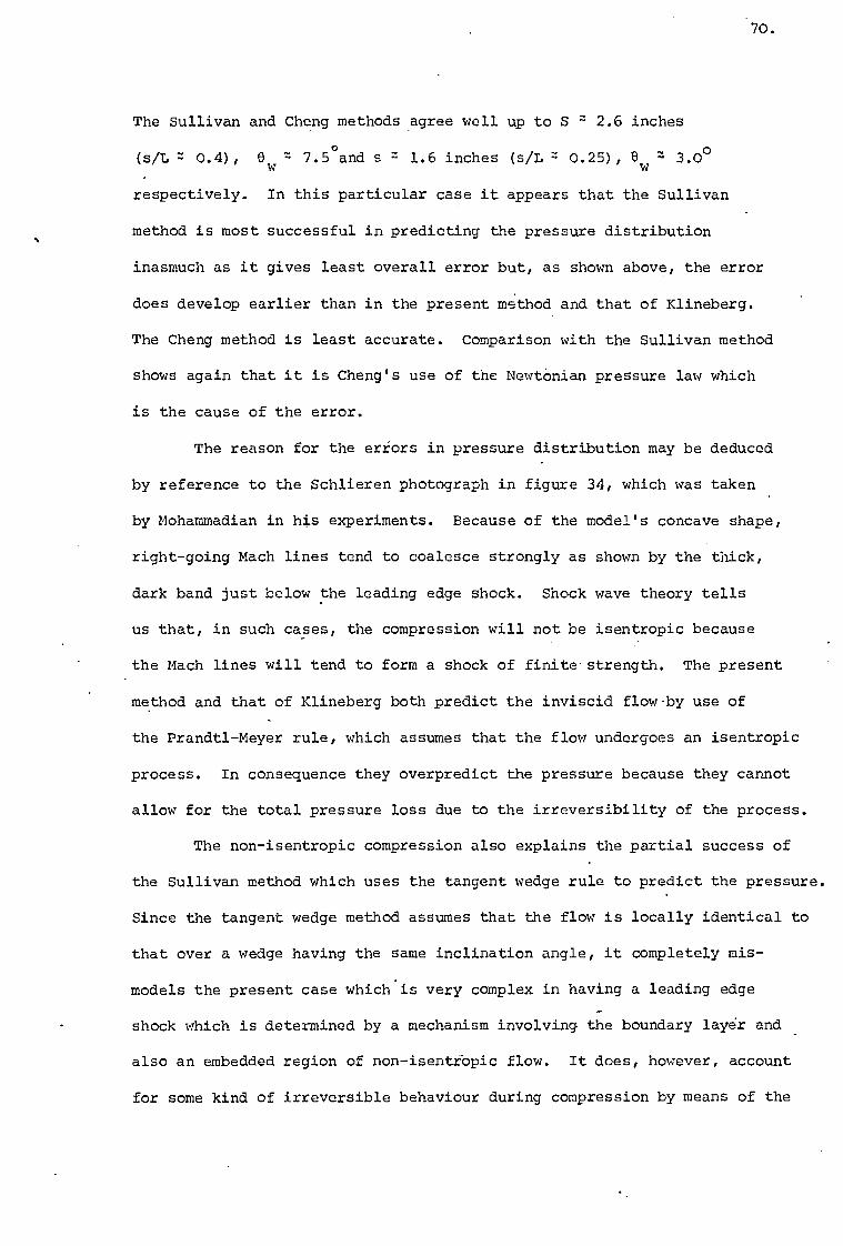
70.
The Sullivan and Cheng methods agree well up to S = 2.6 inches
(s/L 7: 0.4), Ow "4 7.5°and s 7- 1.6 inches (s/L 0.25), Ow 2 3.0°
respectively. In this particular case it appears that the Sullivan
method is most successful in predicting the pressure distribution
inasmuch as it gives least overall error but, as shown above, the error
does develop earlier than in the present method and that of Klineberg.
The Cheng method is least accurate. Comparison with the Sullivan method
shows again that it is Cheng's use of the NewtOnian pressure law which
is the cause of the error.
The reason for the errors in pressure distribution may be deduced
by reference to the Schlieren photograph in figure 34, which was taken
by Mohammadian in his experiments. Because of the model's concave shape,
right-going Mach lines tend to coalesce strongly as shown by the thick,
dark band just below the leading edge shock. Shock wave theory tells
us that, in such cases, the compression will not be isentropic because
the Mach lines will tend to form a shock of finite strength. The present
method and that of Klineberg both predict the inviscid flow-by use of
the Prandtl-Meyer rule, which assumes that the flow undergoes an isentropic
process. In consequence they overpredict the pressure because they cannot
allow for the total pressure loss due to the irreversibility of the process.
The non-isentropic compression also explains the partial success of
the Sullivan method which uses the tangent wedge rule to predict the pressure.
Since the tangent wedge method assumes that the flow is locally identical to
that over a wedge having the same inclination angle, it completely mis-
models the present case which'is very complex in having a leading edge
shock which is determined by a mechanism involving the boundary layer and
also an embedded region of non-isentropic flow. It does, however, account
for some kind of irreversible behaviour during compression by means of the
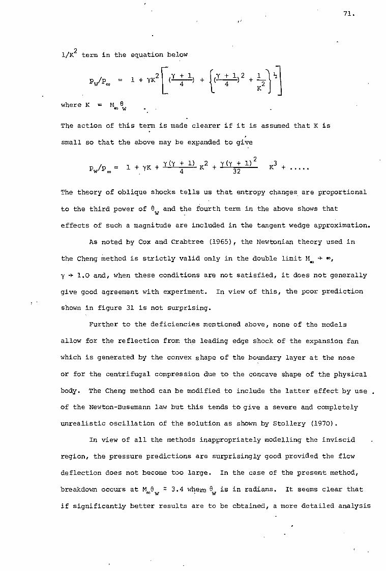
71.
1/K2 term in the equation below
plipm = 1 yK2
where K = M 8 so w
Y 1 y + 1 2 1 )1 ) 4- ( 4 ) --- 4 K2
The action of this term is made clearer if it is assumed that K is
small so that the above may be expanded to give
Pw/p. = 1 + yK (Y + 1) K2 + (y + 1) 2 4 32
K3 K
The theory of oblique shocks tells us that entropy changes are proportional
to the third power of 014 and the fourth term in the above shows that
effects of such a magnitude are included in the tangent wedge approximation.
As noted by Cox and Crabtree (1965), the Newtonian theory used in
the Cheng method is strictly valid only in the double limit M. +so,
y + 1.0 and, when these conditions are not satisfied, it does not generally
give good agreement with experiment. In view of this, the poor prediction
shown in figure 31 is not surprising.
Further to the deficiencies mentioned above, none of the models
allow for the reflection from the leading edge shock of the expansion fan
which is generated by the convex shape of the boundary layer at the nose
or for the centrifugal compression due to the concave shape of the physical
body. The Cheng method can be modified to include the latter effect by use .
of the Newton-Busemann law but this tends to give a severe and completely
unrealistic oscillation of the solution as shown by Stollery (1970).
In view of all the methods inappropriately modelling the inviscid
region, the pressure predictions are surprisingly good provided the flow
deflection does not become too large. In the case of the present method,
breakdown occurs at Mcow 3.4 where 61,4 is in radians. It seems clear that
if significantly better results are to be obtained, a more detailed analysis
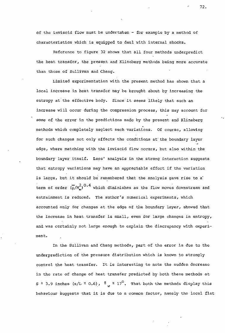
72.
of the inviscid flow must be undertaken - for example by a method of
characteristics which is equipped to deal with internal shocks.
Reference to figure 32 shows that all four methods underpredict
the heat transfer, the present and Klineberg methods being more accurate
than those of Sullivan and Cheng.
Limited experimentation with the present method has shown that a
local increase in heat transfer may be brought about by increasing the
entropy at the effective body. Since it seems likely that such an
increase will occur during the compression process, this may account for
some of the error in the predictions made by the present and Klineberg
methods which completely neglect such variations. Of course, allowing
for such changes not only affects the conditions at- the boundary layer
edge, where matching with the inviscid flow occurs, but also within the
boundary layer itself. Lees' analysis in the strong interaction suggests
that entropy variations may have an appreciable effect if the variation
is large, but it should be remembered that the analysis gave rise to a°
2 0.4 term of order ( /M.) which diminishes as the flow moves downstream and
entrainment is reduced. The author's numerical experiments, which
accounted only for changes at the edge of the boundary layer, showed that
the increase in heat transfer is small, even for large changes in entropy,
and was certainly not large enough to explain the discrepancy with experi-
ment.
In the Sullivan and Cheng methods, part of the error is due to the
underprediction of the pressure distribution which is known to strongly
control the heat transfer. It is interesting to note the sudden decrease
in the rate of change of heat transfer predicted by both these methods at
S 7- 3.9 inches (s/L 2 0.6), w = 17°. That both the methods display this
behaviour suggests that it is due to a common factor, namely the local flat
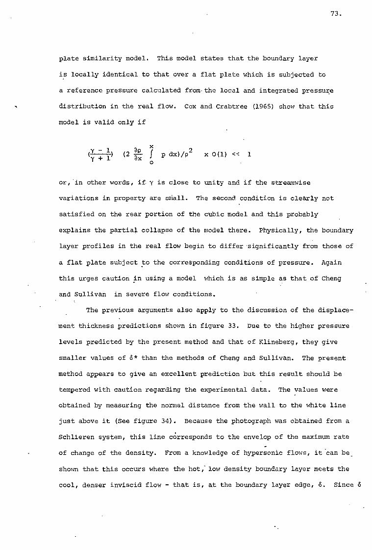
73.
plate similarity model. This model states that the boundary layer
is locally identical to that over a flat plate which is subjected to
a reference pressure calculated from.the local and integrated pressure
distribution in the real flow. Cox and Crabtree (1965) show that this
model is valid only if
(y - 1
) (2 3p— f p dx)/P2 x 0(1) <= 1 y -I- 1 ax 0
or, in other words, if y is close to unity and if the streamwise
variations in property are small. The second condition is clearly not
satisfied on the rear portion of the cubic model and this probably
explains the partial collapse of the model there. Physically, the boundary
layer profiles in the real flow begin to differ -significantly from those of
a flat plate subject to the corresponding conditions of pressure. Again
this urges caution in using a model which is as simple as that of Cheng
and Sullivan in severe flow conditions.
The previous arguments also apply to the discussion of the displace-
ment thickness predictions shown in figure 33. Due to the higher pressure
levels predicted by the present method and that of Klineberg, they give
smaller values of 6* than the methods of Cheng and Sullivan. The present
method appears to give an excellent prediction but this result should be
tempered with caution regarding the experimental data. The values were
obtained by measuring the normal distance from the wall to the white line
just above it (See figure 34). Because the photograph was obtained from a
Schlieren system, this line corresponds to the envelop of the maximum rate
of change of the density. From a knowledge of hypersonic flows, it can be
shown that this occurs where the hot,- low density boundary layer meets the
cool, denser inviscid flow - that is, at the boundary layer edge, 6. Since 6
74.
is little different from (5* in hypersonic flows, the normal distance
may be interpreted as the displacement thicknes. Further to these
assumptions, error may be expected in the measurement of the small dis-
tances from the photograph. Despite this, the good agreement does invite
cautious optimism in the method.
The discussion so far has been limited to effects which are within
the compass of first order boundary layer theory. At hypersonic speeds,
however, second order effects may become important, the principal ones
being due to longitudinal curvature and a non-zero normal pressure gradient
within the boundary layer. The former involves making corrections to the
theoretical model in order to account for the centrifugal forces acting
upon the flow which, according to simple mechanics, increase with the
square of the local velocity. The latter is due to the variations of
velocity across the boundary layer which are necessarily large when the
external stream moves with hypersonic speeds. For a full survey and dis-
cussion of second order boundary layer theory see van Dyke (1969). A
series of calculations which include the second order effects mentioned
above were performed by Wornom and Werle (1972). The boundary layer was
modelled by the full second order equations of motion, which were solved
numerically, and the inviscid flow was modelled by the tangent wedge
method. Interaction was permitted by matching the solutions at the displace=
ment thickness, which was assumed to be a streamline, in the same manner as
the present method. The flows over both the flat plate and the cubic model
was calculated. Because of the small size of the figures in the original
paper and the lack of numerical data, Wornom and Werles' results have not
been plotted on the figures in the present work. Instead the results will
be compared with those given by Sullivan's method as these appear in both
papers.
75.
In the case of the flat plate, the published results show a
general increase in pressure levels of approximately 5-10% over that
predicted by Sullivan. In the case of the cubic model,the same is
true in the region of the leading edge where the body curvature is
small. Further back, as the deflection due to the physical body becomes
more important than that due to the boundary layer, the pressure tends
to that predicted by the Sullivan method, which also uses the tangent
wedge rule in the inviscid region. This work, therefore, suggests that
second order terms tend to increase the predicted pressure, but only
by a small amount.
The paper gives the predicted displacement thickness but only
for the case of the cubic body. These tend to be 5-10 per cent below
those given by the Sullivan method in the region of the leading edge
but 10 - 15 per cent above them in the rear portion of the body.
Wornom and Werle conclude that the second order terms tend to
have a mutually cancelling effect and that the net difference from
first order theory is small. This conclusion is further reinforced by
comparing the velocity profiles predicted by first and second order
theory. At the station s = 1.5" (s/L = 0.23), e w = 2.5° the difference
was very small, 1 per cent at most, whilst at a second station s = 4.5 •
inches (s/L = 0.69), ew = 21.9° the profiles were geometrically similar
in shape but with the second order profile offset so that the velocity
was 10-15 per cent smaller than that given by first order theory at the
same ordinate. The second order theory's prediction of skin friction was
therefore lower than that due to first order theory.
The small influence of second order terms further suggests that
the main reason for the inaccuracy of the present method lies in the mis-
76.
modelling of the inviscid region. As noted earlier, improved results
are to be expected only if this region is analysed more thoroughly.
In comparing the various methods, mention must be made of their
relative economics. Briefly, a typical calculation with the present
method takes 3,000 seconds, one with the Klineberg method takes 120
seconds and one with the Cheng and Sullivan methods takes 3-4 seconds
on a CDC 6600 machine. The methods require 25,000, 40,000 and 20,000
words of central memory respectively. In view of it not producing
significantly better results than the Klineberg method, economics must
rule out the present method for use in an industrial environment,
especially as it requires the use of a £60,000 visual display unit and
human supervision in its present form. It does, however, have the merit
of being a rational approach inasmuch as it can be developed to give
increased accuracy by use of more refined numerical approximations.
Further, it has been written so that such changes can be made easily and
thus, in the author's opinion, it is valuable as a research tool for the
testing of new techniques and theories. In this sense, the Klineberg
approach is not so good and Brown and Stewartson (1969) make a list of
the objections to it in their paper. Despite this, Klineberg's method
has been shown to give good results over a wide range of conditions and,
of course, it can handle the shock-boundary layer interaction successfully.
The Sullivan approach should not be discarded, however, since if it is used
sensibly it can produce good, reliable results at very small cost in
computer resources. In the author's opinion, the Sullivan method makes
an excellent initial design tool whilst the Klineberg method is valuable
for detailed calculations or for analysing difficult flows.
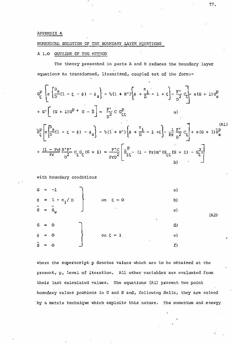
77.
APPENDIX A
NUMERICAL SOLUTION OF THE BOUNDARY LAYER EQUATIONS
A 1.0 OUTLINE OF THE METHOD
The theory presented in parts A and B reduces the boundary layer
equations to transformed, linearised, coupled set of the form:- •I
Gf s -e-(1 - - 4)) - c P sl - ;1(1 + E l + Ili+ - 1
+ G I [ (G + 1)GP + G - ti = 12-y C GP„ D
Ti. - C - - (P, / - 11(1+ E') + - 1
r F ' - D2 s(G + 1))GPs
a)
1 F' (Al)
pr + s (G + 1) SS
(1 - Pr) H'F' C G (G + 1) = F'C SP - (1 - Pr)H' (G (G + 1) - G2 ) Pr D2 PrD2
[- CC
with boundary conditions
G =
=
S =
• -1
1 - ni/ D
sw
on = 0
a)
b)
c)
G = 0 d)
(A2)
=
=
0
0
on = 1 e)
f)
where the superscript p denotes values which are to be obtained at the
present, p, level of iteration. All other variables are evaluated from
their last calculated values. The equations (Al) present two point
boundary values problems in G and S and, following Sells, they are solved
by a matrix technique which exploits this nature. The momentum and energy
b)
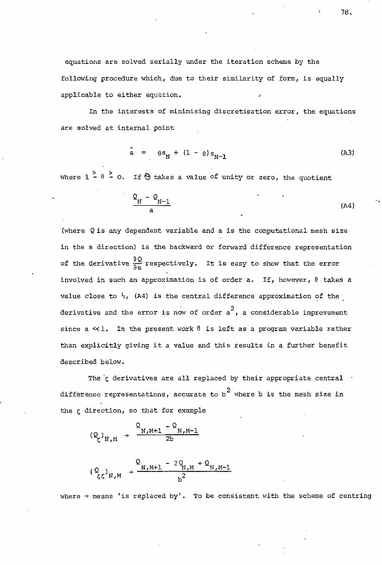
78.
equations are solved serially under the iteration scheme by the
following procedure which, due to their similarity of form, is equally
applicable to either equation.
In the interests of minimising discretisation error, the equations
are solved at internal point
= 8sN + (1 - e)sN_1 (A3)
where 1 > - u > - 0. If et takes a value of unity or zero, the quotient
QN - Q
N -1 (A4) a
(where Q is any dependent variable and a is the computational mesh size
in the s direction) is the backward or forward difference representation
of the derivative 3Q respectively. It is easy to show that the error Ds
involved in such an approximation is of order a. If, however, 8 takes a
value close to 11, (A4) is :the central difference approximation of the
derivative and the error is now of order a2, a considerable improvement
since a <<1. In the present work 8 is left as a program variable rather
than explicitly giving it a value and this results in a further benefit
described below.
The derivatives are all replaced by their appropriate central •
difference representations, accurate to b2 where b is the mesh size in
the direction, so that for example
- QN,M+1
Q N,M-1
(Q ) N,M 2b
N,M+1 29N,M +QN,M-1 (Q ) N,M b
2
where .4- means 'is replaced by'. To be consistent with the scheme of centring
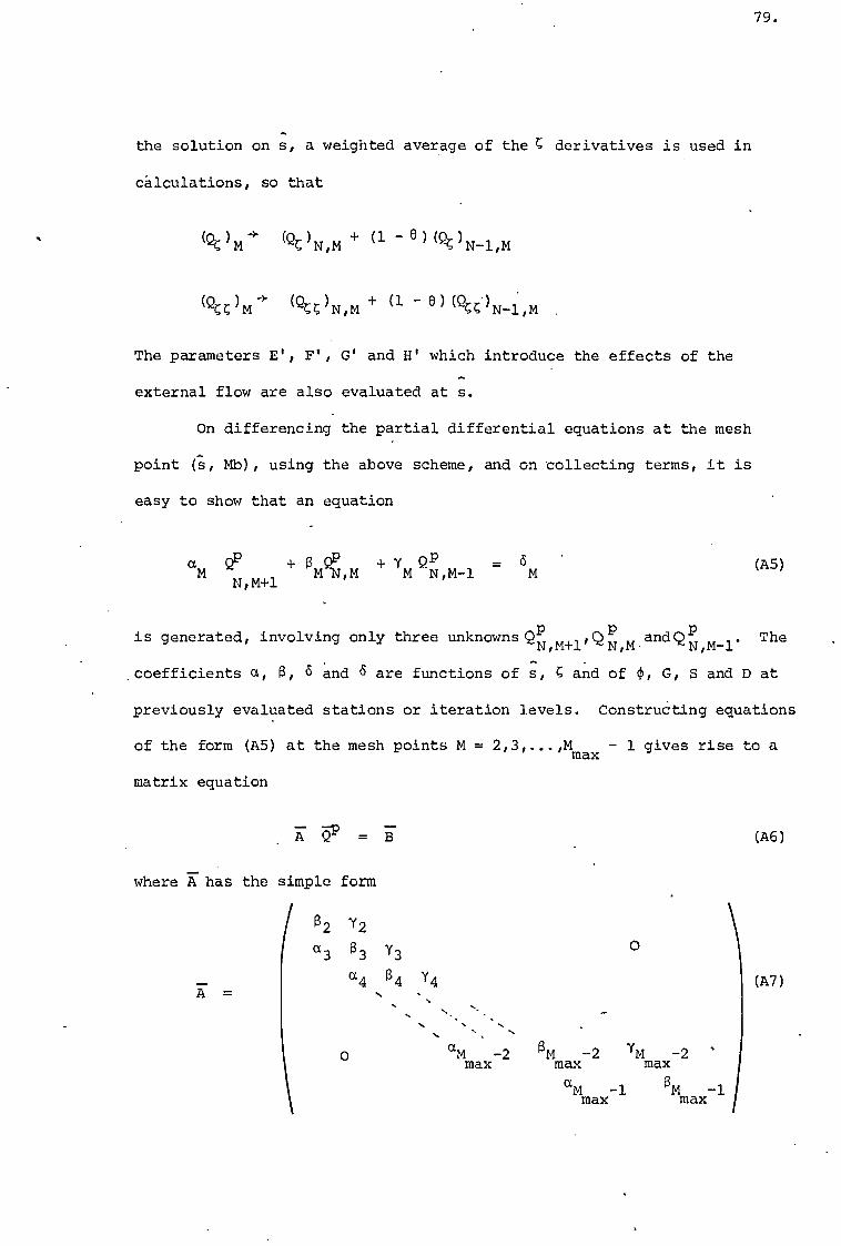
79.
the solution on s, a weighted average of the C derivatives is used in
calculations, so that
(ck ) m (c20 m ,m (1 — ) (Q-0 N-1,m
(Q&m (QcOm,m -1- (1 ) )N-1,M
The parameters E', F', G' and H' which introduce the effects of the
external flow are also evaluated at s.
On differencing the partial differential equations at the mesh
point (s, Mb), using the above scheme, and on collecting terms, it is
easy to show that an equation
am
N,M+1 M
gP __ Om M N,M-1 (A5)
n 17) is generated, involving only three unknowns e N,M+11,,N,m andc)N,m_i. The
.coefficients a, 6 and 6 are functions of s, C and of 1, G, S and D at
previously evaluated stations or iteration levels. Constructing equations
of the form (A5) at the mesh points M = 2,3,—"Mmax 1 gives rise to a
matrix equation
;51) = (A6)
where A has the simple form
2 Y2
°3 13 0
= a4 134 y4 (A7)
•
0
aM -2 am. -2 YM -2 max max max
aMmax-1 SM Max-1
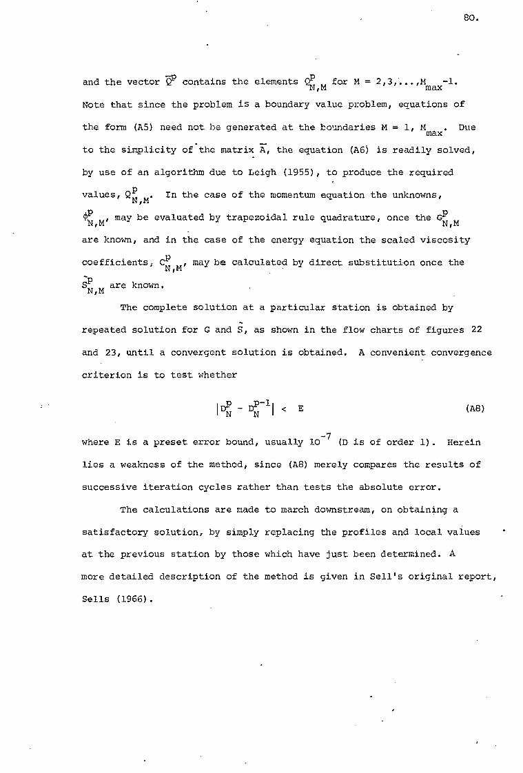
80.
and the vector V° contains the elements Q1:1 ,,,1 for M = 2,3,...,Mmax-1.
Note that since the problem is a boundary value problem, equations of
the form (A5) need not be generated at the boundaries M = 1, Mmax. Due
to the simplicity of.the matrix A, the equation (A6) is readily solved,
by use of an algorithm due to Leigh (1955), to produce the required
values, M'
QP In the case of the momentum equation the unknowns, N
(f)P , may be evaluated by trapezoidal rule quadrature, once the GP ,M N,M
are known, and in the case of the energy equation the scaled viscosity
coefficients,
JP M
C,M- , may be calculated by direct substitution once the
N
are known. N,
The complete solution at a particular station is obtained by
repeated solution for G and S, as shown in the flow charts of figures 22
and 23, until a convergent solution is obtained. A convenient convergence
criterion is to test whether
Dp - Dp 11 < E
N N (A8)
where E is a preset error bound, usually 10-7 (D is of order 1). Herein
lies a weakness of the method, since (A8) merely compares the results of
successive iteration cycles rather than tests the absolute error.
The calculations are made to march downstream, on obtaining a
satisfactory solution, by simply replacing the profiles and local values
at the previous station by those which have just been determined. A
more detailed description of the method is given in Sell's original report,
Sells (1966).
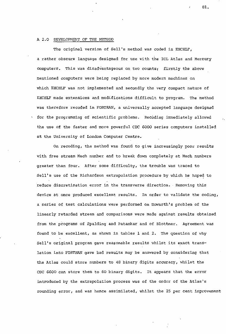
81.
A 2.0 DEVELOPMENT OF THE METHOD
The original version of Sell's method was coded in EXCHLF,
a rather obscure language designed for use with the ICL Atlas and Mercury
computers. This was disadvantageous on two counts; firstly the above
mentioned computers were being replaced by more modern machines on
which EXCHLF was not implemented and secondly the very compact nature of
EXCHLF made extensions and modifications difficult to program. The method
was therefore recoded in FORTRAN, a universally accepted language designed
- for the programming of scientific problems. Recoding immediately allowed
the use of the faster and more powerful CDC 6000 series computers installed
at the University of London Computer Centre.
On recoding, the method was found to give increasingly poor results
with free stream Mach number and to break down completely at Mach numbers
greater than four. After some difficulty, the trouble was traced to
Sell's use of the Richardson extrapolation procedure by which he hoped to
reduce discretisation error in the transverse direction. Removing this
device at once produced excellent results. In order to validate the coding,
a series of test calculations were performed on Howarth's problem of the
linearly retarded stream and comparisons were made against results obtained
from the programs of Spalding and Patankar and of Blottner. Agreement was
found to be excellent, as shown in tables 1 and 2. The question of why
Sell's original program gave reasonable results whilst its exact trans-
lation into FORTRAN gave bad results may be answered by considering that
the Atlas could store numbers to 48 binary digits accuracy, whilst the
CDC 6600 can store them to 60 binary digits. It appears that the error
introduced by the extrapolation process was of the order of the Atlas's
rounding error, and was hence assimilated, whilst the 25 per cent improvement
82.
of accuracy on the 6600 allowed the error to exert its influence
proper and so destroy the solution. A benefit arising from dispensing
with the extrapolation process is that the program now requires less.
running time and memory space since the need for calculating each
station twice and storing the partial results is obviated.
The method was further developed, in the course of the present
work, by allowing for the effects of an entropy at the 'edge' of the
boundary layer, le, different to that of the free stream, by modifying
the expressions for E', F', G' and H', the pressure gradient parameters,
and the equations for Cf147, St 1/17; and d*/sATIE: as described in
equations (6.16), (6.22), (6.42), (6.44) and (6.47) of part B. By means
of such modifications, the method is extended for use in situations where
the flow passes through a shock wave before the'boundary layer develops.
As noted in table 2, Sells method breaks down in the case of
Tw = T for free stream Mach numbers greater than 14. Examination of
velocity and enthalpy profiles in the transformed plane show that this
is due to the computational mesh being too small to allow boundary layer
growth away from the leading edge region. The problem cannot be resolved
by simply choosing a larger value for ni, the boundary layer thickness
parameter, because this affects the whole of the mesh. The problem then
moves from the downstream region to the leading edge where the mesh
becomes too coarse to allow a successful solution. It appears that ni
needs to be adjusted step by step so as to allow for the growth but it
is not easy to see how this can be done within the present formulation of
the problem.

83.
APPENDIX B
B 1.0 INTRODUCTION
The method,as described in part B,takes a specification of the
free stream conditions, the model geometry and wall-temperature and a
set of history profiles as input and produces a set of new profiles and
results at the new station as output. The question of how to generate
the first set of history profiles, from which to start the full solution,
is treated here. In order to avoid theoretical and computational problems,
no attempt is made to calculate the flow very close to the origin, s = 0,
using the previously described approach, but instead results from strong
interaction theory are used and the main program is started from them at
x = 12. Specifically, the pressure ratio (32e/p) as a function of X, the
strong interaction parameter, is assumed and the details of the viscous
and inviscid regions are calculated from it. This technique should give
good results within the range of validity of strong interaction theory
(see figure 24) but not at very high values of X, where, physically, a
merged shock wave-boundary layer exists. The problem of obtaining a
valid solution in this region is beyond the scope of the present work,
but instead the region is used to overcome difficulties arising from the
infinite pressure at s = O,predicted by strong interaction theory,and so
produce a solution which will lead smoothly and consistently into that
given by strong interaction theory.
B 2.0 THEORY
B 2.1 THE INVISCID REGION
The pressure distribution at the edge of the boundary layer, according
to strong interaction theory is given by
Pe/Pc = Pox - (1 + P1 (B1)
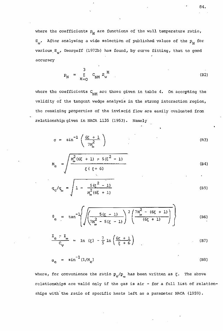
84.
where the coefficients pN are functions of the wall temperature ratio,
S w. After analysing a wide selection of published values of the pN
for
various Sw, Georgeff (1972b) has found, by curve fitting, that to good
accuracy
3 M p
N =ECS M=0 NM W
where the coefficients CNM are those given in table 4. On accepting the
validity of the tangent wedge analysis in the strong interaction region,
the remaining properties of the inviscid flow are easily evaluated from
relationshipsgiven in NACA 1135 (1953). Namely
= sin— (6g + c 2 7Mo,
(F33)
Me + 1) r 5(g 2 - 1)
(B4) g( + 6)
clj
5 2 — 1) e/ c1 = 1 Me, (6 + 1)
(B2)
(B5)
= tan
e 7M2 — 5 — 1)
5 Q — 1) ) 2 ( 7M2 — (6g + 1)) (6 + 1) ( co -1
(B6)
(B7)
(B8)
I r I co e
7 ( 6 2.:..1. ) In T - in - -I- 6 Cv
ae = sin-1
(1/Me)
where, for convenience the ratio pe/pm has been written as E. The above
relationships are valid only if the gas is air - for a full list of relation-
ships with.the ratio of specific heats left as a parameter NACA (1959).
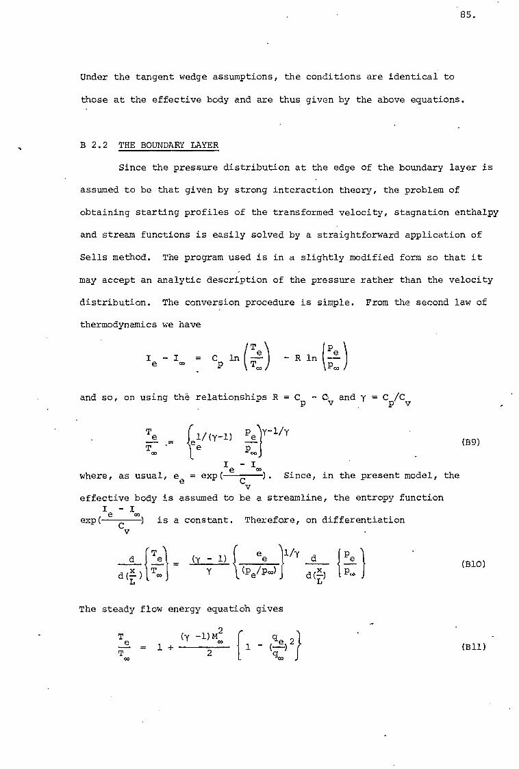
85.
Under the tangent wedge assumptions, the conditions are identical to
those at the effective body and are thus given by the above equations.
B 2.2 THE BOUNDARY LAYER
Since the pressure distribution at the edge of the boundary layer is
assumed to be that given by strong interaction theory, the problem of
obtaining starting profiles of the transformed velocity, stagnation enthalpy
and stream functions is easily solved by a straightforward application of
Sells method. The program used is in a slightly modified form so that it
may accept an analytic description of the pressure rather than the velocity
distribution. The conversion procedure is simple. From the second law of
thermodynamics we have
Pp
I
e
- 1 = C In - R ln p T00 Poo
and so, on using the relationships R = C - 0 and y = C /C P v p v
Te pely-1/y
1/(y-1) 17— -= Pc.
I - e
where, as usual, ee = exp( c ). Since, in the present model, the v
effective body is assumed to be a streamline, the entropy function I e C 00 - I
exp( is a constant. Therefore, on differentiation v
l/y d [Ire) (y - 1) ee d 1
d ) T., Y (Pe/P00) d P.c. (no)
The steady flow energy equatioh gives
Te (y -1)M! f cle 21 = 1 +
2 1 - (B11)
(B9)
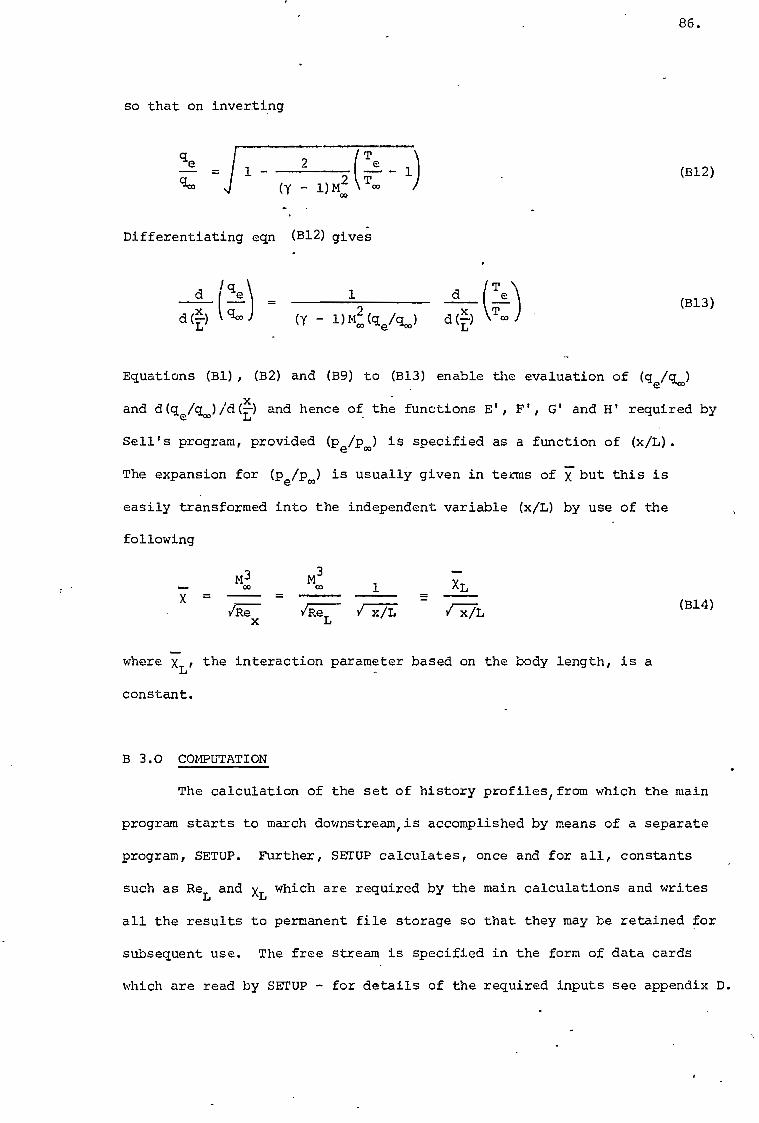
86.
so that on inverting
qe T = 1
e 2 1
goo 2 (T (y - 1)mm co
(312)
Differentiating eqn (B12) gives
d I/ q
e 1 d (Te)
deL-c-) Cie° (Y
1 ) Mco
im
( e goo ) d(L) T. (B13)
Equations (B1), (B2) and (B9) to (B13) enable the evaluation of (qe/q.)
and d(qe/q.)/d() and hence of the functions E', F', G' and H' required by
Sell's program, provided (pe/p.) is specified as a function of (x/L).
The expansion for (pe/p.) is usually given in terms of T but this is
easily transformed into the independent variable (x/L) by use of the
following
M3 M3 co 1 XL X = v-E7- 17717 [7L
(314)
where XL, the interaction parameter based on the body length, is a
constant.
B 3.0 COMPUTATION
The calculation of the set of history profiles/ from which the main
program starts to march downstream/ is accomplished by means of a separate
program, SETUP. Further, SETUP calculates, once and for all, constants
such as ReL and XL which are required by the main calculations and writes
all the results to permanent file storage so that they may be retained for
subsequent use. The free stream is specified in the form of data cards
which are read by SETUP - for details of the required inputs see appendix D.
87.
In order to use Sell's program's ability to generate its own
starting solution, calculations must begin at the station s = 0. This,
however, raises a computational problem since at the origin there are
infinities in pe and its x derivative. The problem is surmounted by
setting these variables to large but otherwise arbitrary values. The
profiles so calculated will be in error but the property, by which the
boundary layer equations quickly relax to the solution consistent with
a specified pressure distribution from any other neighbouring solution,
is exploited to obtain a good solution before the strong interaction
region is reached. This is done by accepting the spurious solution at
the origin and then calculating solutions at a large number of stations
before reaching the strong interaction region (50 in the present version
of the program) under the correct pressure distribution. The procedure
was validated by performing a series of calculations, each identical
except for the number of stations used in the merged region, from which
it was found that sixth significant figure agreement could be obtained
between solutions, provided more than 25 stations were calculated. This
strongly suggests that the solution does, in fact, tend to the true solution
despite the inaccuracy at the origin.
Twenty five stations were calculated in the strong interaction region
which, for the purposes of programming SETUP, was defined by
25 > - X > - 12
From the above, it is clear that SETUP produces results at seventy five
stations (50 in the merged region and 25 in the strong interaction region)
in the small region bounded by the origin and the station where x = 12.
However, in order that it can run in a modest segment of computer memory,
the main program will allow data to be stored at only 105 streamwise stations.

88.
To overcome the problem of overspecification of the solution close to
the nose, SETUP interpolates within the calculated values to produce data
for retention at the stations whose s co-ordinate is a multiple of As (DELS),
an input parameter, and also at the final station, X = 12. A further
difficulty arising from the data is that, due to the nature of the
prescribed pressure distribution, most of the results have abnormally
large values at the origin and this tends to result in poorly scaled
graphs both at the graphics console and in the output of the Calcomp
plotter. The problem is simply overcome by setting the results at the
origin to be identical to those at the second station, s = As - abandoning
the calculated data at the origin is no great loss since it is clear from
the foregoing that it was derived by a quite arbitrary process.
As described above, strong interaction theory is used to solve the
flow for X - 12 and its results are used to start the present method at
X = 12. The choice- of the starting station and its effect on the subsequent •
calculations is discussed briefly below.
Because strong interaction theory differs in its assumptions and
approximations from the present method, a solution generatedly the
former method will not be completely compatible with the latter. Looking
at this from the point of view of the present method, the initial data
will already contain disturbing perturbations and so that any solution com-
puted from it will immediately diverge from the true solution. As outlined
by Georgeff (1972a), the rate at which a solution diverges depends upon
both the formulation of the method and on the local conditions. A series
of test calculations has shown that, by means of latter influence, the
present method is prone to increasing divergence with increasing X. As a -
result, if calculations are started at too large a value of x, the combined
effect of the perturbations in the initial data and the large rate of diver-
89.
gence is to prevent the calculation of a smooth solution, if a five
significant figure controlling perturbation is used as in the present
method. Presumably, if the controlling perturbation was allowed to have
a finer resolution, by specifying it to a greater number of significant
figures, a smooth solution could be obtained, but programming considera-
tions ruled this out. It was found that, by selecting an initial station
with a reduced X , a smooth solution, which was initially offset from the
true solution but which quickly tended to it, could be produced as shown
schematically in figure 35. The smaller the 5(, the smaller the offset
and the quicker the solution tended to the true solution. A compromise
between starting the full solution as early as possible whilst minimising
the error due to offset resulted in a choice of 7= 12 for the initial
station in the present cases.
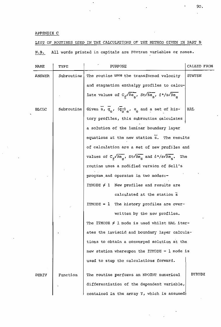
90.
APPENDIX C
LIST OF ROUTINES USED IN THE CALCULATIONS OF THE METHOD GIVEN IN PART B
All words printed in capitals are Fcrtran variables or names.
TYPE PURPOSE
CALLED FROM
The routine uses the transformed velocity STWTSN
and stagnation enthalpy profiles to calcu-
late values of C Res, St f s'
Given s, qe, (q--s)
e , e e
and a set of his- HAL
tory profiles, this subroutine calculates
N.B.
NAME
ANSWER
BLCLC
a solution of the laminar boundary layer
equations at the new station s. The results
of calculation are a set of new profiles and
values of Cflic, Stfit..e7; and Pr/s147. The
routine uses a modified version of Sell's
program and operates in two modes:-
ITMODE 1 New profiles and results are
calculated at the station "g
ITMODE = 1 The history profiles are over-
written by the new profiles.
The ITMODE 1 mode is used whilst HAL iter-
ates the inviscid and boundary layer calcula-
tions to obtain a converged solution at the
new station whereupon the ITMODE = 1 mode is
used to step the calculations forward.
DERIV The routine performs an NPOINT numerical
differentiation of the dependent variable,
contained in the array Y, which is assumed
Subroutine
Subroutine
Function DYBYDX
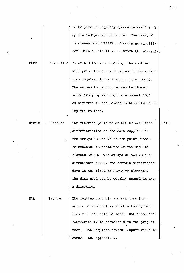
91.
to be given in equally spaced intervals, H,
of the independent variable. The array Y
is dimensioned,NARRAY and contains signifi-
cant data in its first to NDATA th. elements
Subroutine As an aid to error tracing, the routine
will print the current values of the varia-
bles required to define an initial point.
The values to be printed may be chosen
selectively by setting the argument IBUF
as directed in the comment statements head-
ing the routine.
Function The function performs an NPOINT numerical
differentiation on the data supplied in
the arrays XE and YE at the point whose x
co-ordinate is contained in the NANS th
element of XE. The arrays XE and YE are
dimensioned NARRAY and contain significant
data in the first to NDATA th elements.
The data need not be equally spaced in the
x direction.
Program The routine controls and monitors the
action of subroutines which actually per-
form the main calculations. HAL also uses
subroutine TV to converse with-the program
user. HAL requires several inputs via data
cards. See appendix D.
SETUP
DUMP
DYBYDX
HAL
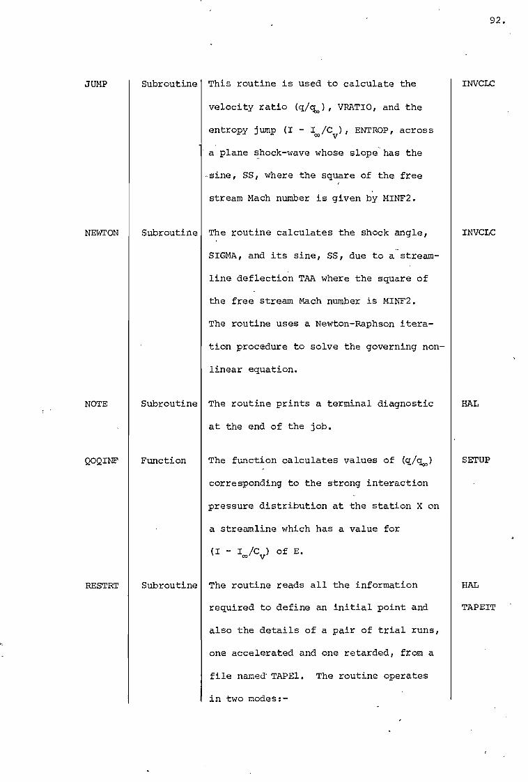
92.
This routine is used to calculate the
velocity ratio (q/q,), VRATIO, and the
entropy jump (I - Im/Cv), ENTROP, across
a plane shock-wave whose slope has the
sine, SS, where the square of the free
stream Mach number is given by MINF2.
The routine calculates the shock angle,
SIGMA, and its sine, SS, due to a stream-
line deflection TAA where the square of
the free stream Mach number is MINF2.
The routine uses a Newton-Raphson itera-
tion procedure to solve the governing non-
linear equation.
Subroutine
Subroutine
Subroutine The routine prints a terminal diagnostic
at the end of the job.
The function calculates values of (q/qm)
corresponding to the strong interaction
pressure distribution at the station X on
a streamline which has a value for
(I - Iw/Cv) of E.
The routine reads all the information
required to define an initial point and
also the details of a pair of trial runs,
one accelerated and one retarded, from a
file named' TAPEl. The routine operates
in two modes:-
Function
Subroutine
INVCLC
INVCLC
HAL
SETUP
HAL
TAPEIT °
JUMP
NEWTON
NOTE
QOQINF
RESTRT

93.
MODEOP 1 All data is read from TAPE1
MODEOP = 1 All data except details of
the trial runs is read from
TAPE1.
BLCLC
TV
SETUP
The routine calculates values propor-
tional to CI ,...(F s, stA77, 6*/s/E7
at each new station from the new profile
SETUP is used to calculate the initial
pointpfrom which the program HAL makes
its calculations1 by means of results
from strong interaction theory. All inter-
mediate results are relayed to HAL by
means of permanent file storage devices.
SETUP requires the specification of the
free stream by means of the data cards shown
in appendix D.
Given the maximum value of a variable,
VALUE, this routine calculates a suitable
size of axis, AXIS, and a suitable incre-
ments for the scale markings on that axis,
STEP, so that the data may be displayed
to the best advantage.
This routine is used to calculate the
laminar boundary layer under a pressure
distribution given by strong interaction
theory. The transformed profiles of
RESULT
Subroutine
SETUP
Program
SIZE
Subroutine
STWTSN
Subroutine
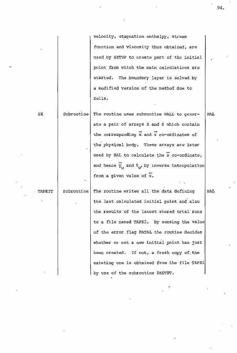
94.
velocity, stagnation enthalpy, stream
function and viscosity thus obtained, are
used by SETUP to create part of the initial
point from which the main calculations are
started. The boundary layer is solved by
a modified version of the method due to
Sells.
The routine uses subroutine WALL to gener-
ate a pair of arrays X and S which contain
the corresponding x and s co-ordinates of
the physical body. These arrays are later
used by HAL to calculate the x co-ordinate,
and hence yti! andw,by inverse interpolation
from a given value of s.
HAL
The routine writes all the data defining
HAL
the last calculated initial point and also
the results of the latest stored trial runs
to a file named TAPE2. By sensing the value
of the error flag FATAL the routine decides
whether or not a new initial point has just
been created. If not, a fresh copy of.the
existing one is obtained from the file TAPE1
by use of the subroutine RESTRT.
SX
Subroutine
TAPEIT
Subroutine
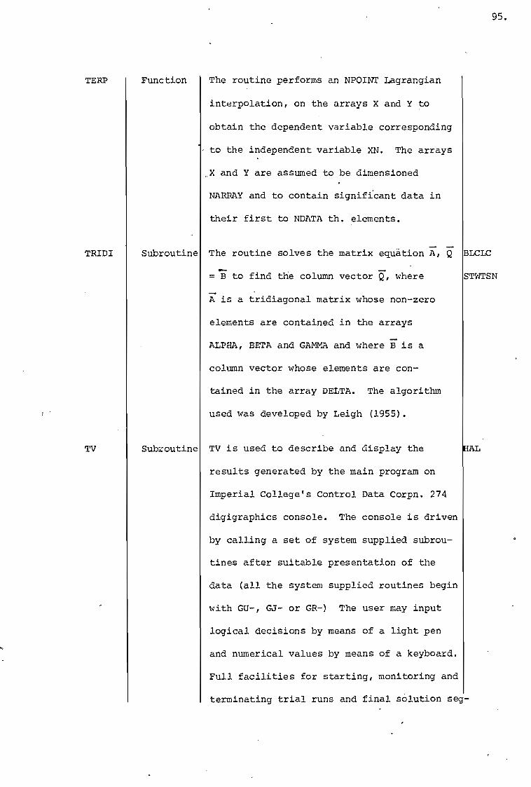
95.
The routine performs an NPOINT Lagrangian
interpolation, on the arrays X and Y to
obtain the dependent variable corresponding
- to the independent variable XN. The arrays
o X and Y are assumed to be dimensioned
NARRAY and to contain significant data in
their first to NDATA th. elements.
— — The routine solves the matrix equation A, Q BLCLC
= B to find the column vector Q, where STWTSN
A is a tridiagonal matrix whose non-zero
elements are contained in the arrays
ALPHA, BETA and GAMMA and where B is a
column vector whose elements are con-
tained in the array DELTA. The algorithm
used was developed by Leigh (1955).
TV is used to describe and display the I
results generated by the main program on
Imperial College's Control Data Corpn. 274
digigraphics console. The console is driven
by calling a set of system supplied subrou-
tines after suitable presentation of the
data (all the system supplied routines begin
with GU-, GJ- or GR-) The user may input
logical decisions by means of a light pen
and numerical values by means of a keyboard.
Full facilities for starting, monitoring and
terminating trial runs and final solution seg-
TERP
Function
TRIDI
Subroutine
TV
Subroutine

96.
ments are provided at the console. See
g7.2 for full details.
This routine contains the shape of the
physical body over which the flow is to
be calculated. The user is required to
supply Fortran expressionsfor the wall
ordinate, Y, and gradient, GRAD, in terms
of the cartesian n co-ordinate X.
Reference to appendix A shows that on
solving the boundary layer equations
numerically, a tridiagonal matrix A and
a column vector B are produced whose ele-
ments are functions of previously calcu-
lated quantities. COEFG calculates the
elements of the matrices produced on differ-
encing the momentum equation and stores
them in the arrays ALPHA, BETA, GAMMA and
DELTA.
This routine performs the same function as
COEFG except that the elements are those
obtained by differencing the energy
equation.
QUADT integrates the transformed velocity
profile to produce a transformed stream
function profile by means of a trapezoidal
rule quadrature.
WALL
Subroutine
COEFG
Subroutine
COEFK
Subroutine
QUADT
Subroutine
HAL
SETUP
TV
BLCLC
STWTSN
BLCLC
STWTSN
BLCLC
STWTSN
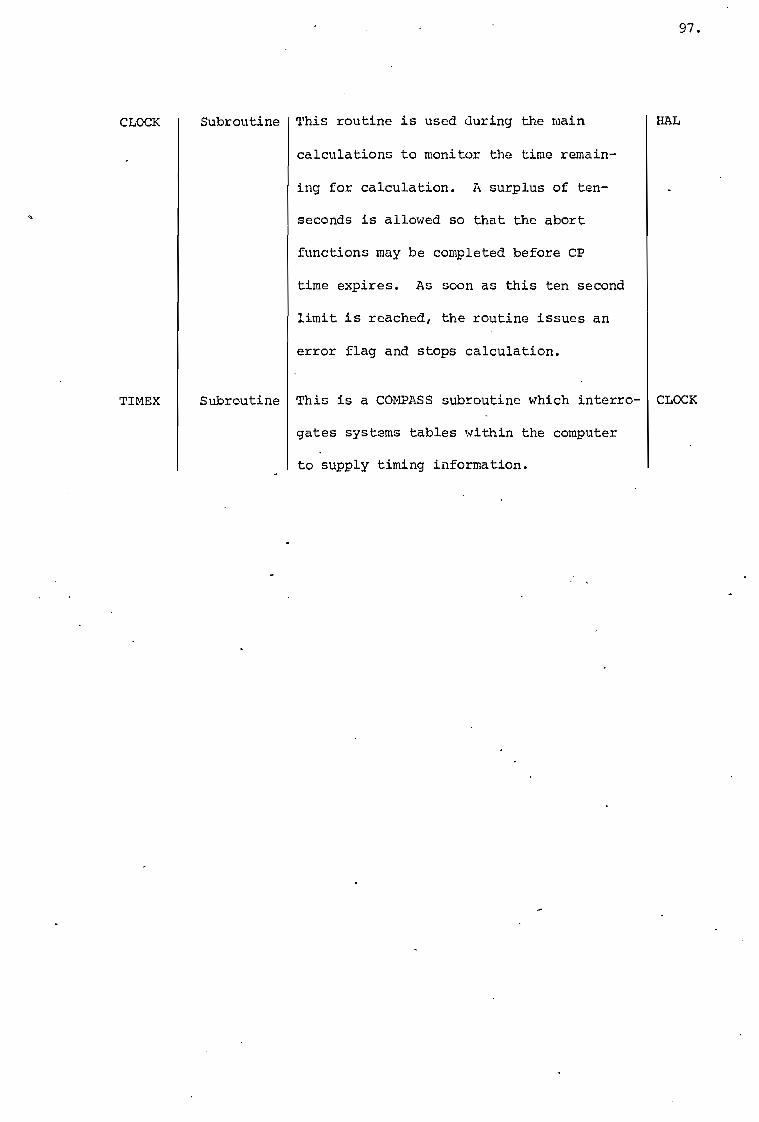
97.
This routine is used during the main
calculations to monitor the time remain-
ing for calculation. A surplus of ten-
seconds is allowed so that the abort
functions may be completed before CP
time expires. As soon as this ten second
limit is reached, the routine issues an
error flag and stops calculation.
This is a COMPASS subroutine which interro-
gates systems tables within the computer
to supply timing information.
CLOCK
Subroutine
TIMEX
Subroutine
HAL
CLOCK
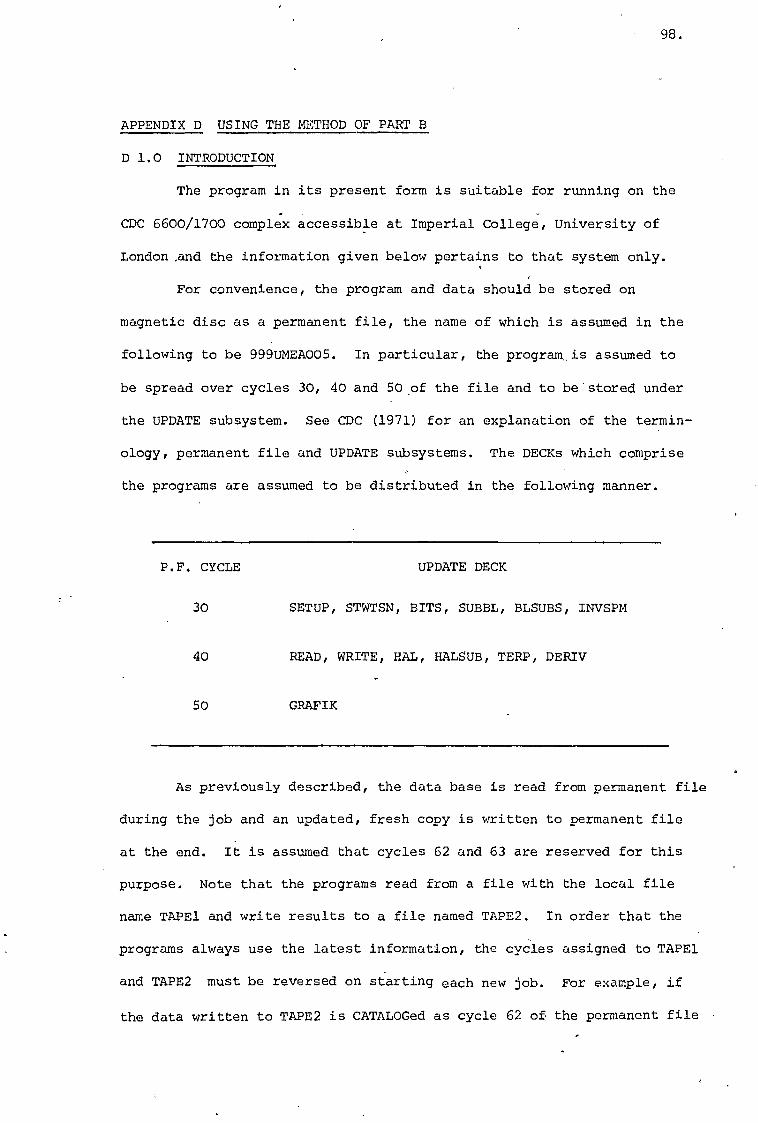
98.
APPENDIX D USING THE METHOD OF PART B
D 1.0 INTRODUCTION
The program in its present form is suitable for running on the
CDC 6600/1700 complex accessible at Imperial College, University of
London And the information given below pertains to that system only.
For convenience, the program and data should be stored on
magnetic disc as a permanent file, the name of which is assumed in the
following to be 999UMEA005. In particular, the program., is assumed to
be spread over cycles 30, 40 and 50 .of the file and to be stored under
the UPDATE subsystem. See CDC (1971) for an explanation of the termin-
ology, permanent file and UPDATE subsystems. The DECKs which comprise
the programs are assumed to be distributed in the following manner.
P.F. CYCLE UPDATE DECK
30 SETUP, STWTSN, BITS, SUBBL, BLSUBS, INVSPM
40 READ, WRITE, HAL, HALSUB, TERP, DERIV
50 GRAFIK
As previously described, the data base is read from permanent file
during the job and an updated, fresh copy is written to permanent file
at the end. It is assumed that cycles 62 and 63 are reserved for this
purpose. Note that the programs read from a file with the local file
name TAPE1 and write results to a file named TAPE2. In order that the
programs always use the latest information, the cycles assigned to TAPE1
and TAPE2 must be reversed on starting each new job. For example, if
the data written to TAPE2 is CATALOGed as cycle 62 of the permanent file
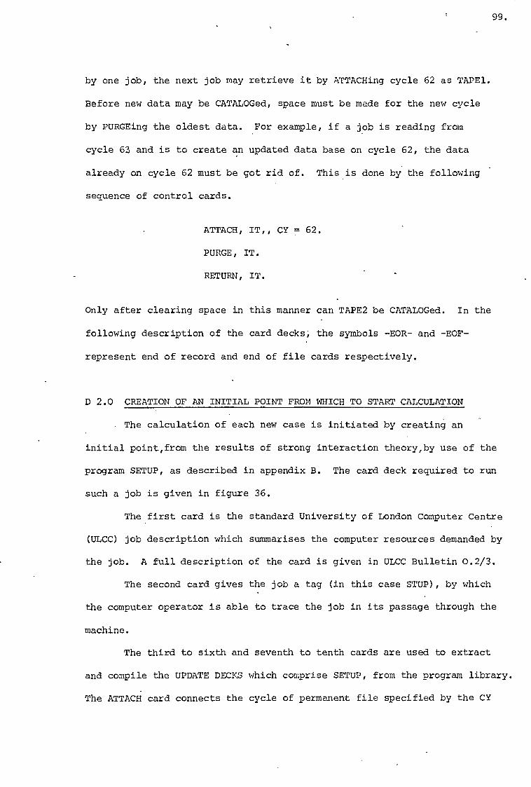
99.
by one job, the next job may retrieve it by ATTACHing cycle 62 as TAPE1.
Before new data may be CATALOGed, space must be made for the new cycle
by PURGEing the oldest data. For example, if a job is reading from
cycle 63 and is to create an updated data base on cycle 62, the data
already on cycle 62 must be got rid of. This is done by the following
sequence of control cards.
ATTACH, IT„ CY = 62.
PURGE, IT.
RETURN, IT.
Only after clearing space in this manner can TAPE2 be CATALOGed. In the
following description of the card decks, the symbols -EOR- and -EOF-
represent end of record and end of file cards respectively.
D 2.0 CREATION OF AN INITIAL POINT FROM WHICH TO START CALCULATION
The calculation of each new case is initiated by creating an
initial point,from the results of strong interaction theory,by use of the
program SETUP, as described in appendix B. The card deck required to run
such a job is given in figure 36.
The first card is the standard University of London Computer Centre
(ULCC) job description which summarises the computer resources demanded by
the job. A full description of the card is given in ULCC Bulletin 0.2/3.
The second card gives the job a tag (in this case STUP), by which
the computer operator is able to trace the job in its passage through the
machine.
The third to sixth and seventh to tenth cards are used to extract
and compile the UPDATE DECKS which comprise SETUP, from the program library.
The ATTACH card connects the cycle of permanent file specified by the CY
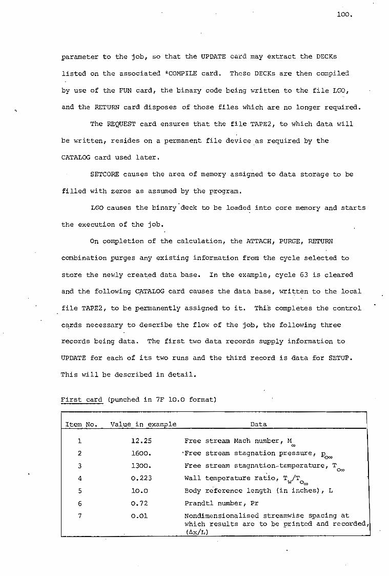
100.
parameter to the job, so that the UPDATE card may extract the DECKS
listed on the associated *COMPILE card. These DECKs are then compiled
by use of the FUN card, the binary code being written to the file LGO,
and the RETURN card disposes of those files which are no longer required.
The REQUEST card ensures that the file TAPE2, to which data will
be written, resides on a permanent file device as required by the
CATALOG card used later.
SETCORE causes the area of memory assigned to data storage to be
filled with zeros as assumed by the program.
LGO causes the binary deck to be loaded into core memory and starts
the execution of the job.
On completion of the calculation, the ATTACH, PURGE, RETURN
combination purges any existing information from the cycle selected to
store the newly created data base. In the example, cycle 63 is cleared
and the following CATALOG card causes the data base, written to the local
file TAPE2, to be permanently assigned to it. This completes the control
cards necessary to describe the flow of the job, the following three
records being data. The first two data records supply information to
UPDATE for each of its two runs and the third record is data for SETUP.
This will be described in detail.
First card (punched in 7F 10.0 format)
Item No. Value in example Data
1 2
12.25
1600.
Free stream Mach number, M co .Free stream stagnation pressure, pom
3 1300. Free stream stagnation-temperature, To=
4 0.223 Wall temperature ratio, Tw/Too,
5 10.0 Body reference length (in inches), L
6 0.72 Prandtl number, Pr
7 0.01 Nondimensionalised streamwise spacing at which results are to be printed and recorded, (ix/L)
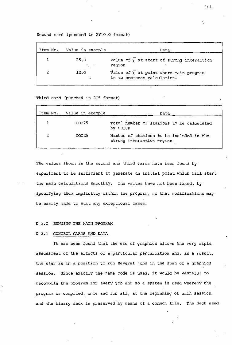
101.
Second card (punched in 2F10.0 format)
Item No. Value in example Data
1 25.0 Value of x at start of strong interaction region
2
12.0 Value of X at point where main program is to commence calculation.
Third card (punched in 215 format)
Item No. Value in example Data
1 00075 Total number of stations to be calculated by SETUP
2
00025 Number of stations to be included in the strong interaction region
The values shown in the second and third cards - have been found by
experiment to be sufficient to generate an initial point which will start
the main calculations smoothly. The values have not been fixed, by
specifying them implicitly within the program, so that modifications may
be easily made to suit any exceptional cases.
D 3.0 RUNNING THE MAIN PROGRAM
D 3.1 CONTROL CARDS AND DATA
It has been found that the use of graphics allows the very rapid
assessment of the effects of a particular perturbation and, as a result,
the user is in a position to run several jobs in the span of a graphics
session. Since exactly the same code is used, it would be wasteful to
recompile the program for every job and so a system is used whereby the
program is compiled, once and for all, at the beginning of each session
and the binary deck is preserved by means of a common file. The deck used
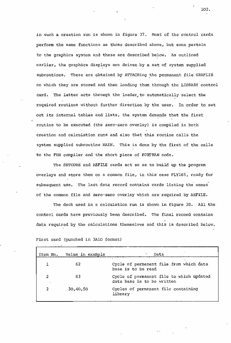
102.
in such a creation run is shown in figure 37. Most of the control cards
perform the same functions as those described above, but some pertain
to the graphics system and these are described below. As outlined
earlier, the graphics displays are driven by a set of system supplied
subroutines. These are obtained by ATTACHing the permanent file GRAFLIB
on which they are stored and then loading them through the LIBRARY control
card. The latter acts through the loader,to automatically select the
required routines without further direction by the user. In order to set
out its internal tables and lists, the system demands that the first
routine to be executed (the zero-zero overlay) is compiled in both
creation and calculation runs and also that this routine calls the
system supplied subroutine MAIN. This is done by the first of the calls
to the FUN compiler and the short piece of FORTRAN code.
The SETCORE and AEFILE cards act so as to build up the program
overlays and store them on a common file, in this case FLY165, ready for
subsequent use. The last data record contains cards listing the names
of the common file and zero-zero overlay which are required by AEFILE.
The deck used in a calculation run is shown in figure 38. All the
control cards have previously been described. The final record contains
data required by the calculations themselves and this is described below.
First card (punched in 3A10 format)
Item No. Value in example Data
1 62 Cycle of permanent file from which data base is to be read
2 63 Cycle of permanent file to which updated data base is to be written
3 30,40,50 Cycles of permanent file containing library
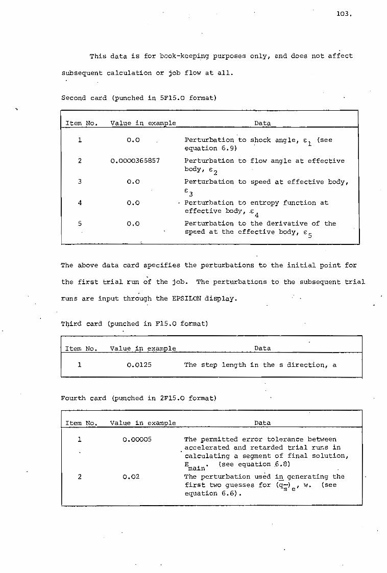
Item No. Value in example
1 0.0
2 0.0000365857
3 0.0
4 0.0
5 0.0
Data
Perturbation to shock angle, el (see equation 6.9)
Perturbation to flow angle at effective body, e2
Perturbation to speed at effective body, e3
- Perturbation to entropy function at effective body, e4
Perturbation to the derivative of the speed at the effective body, e5
The permitted error tolerance between accelerated and retarded trial runs in
of final solution, ,6.8)
calculating a segment E. (see equation main
1 0.00005
2 0.02 The perturbation used first two guesses for equation 6.6).
in generating the (q-E)e, w. (see
Item No. Value in example Data
103.
This data is for book-keeping purposes only, and does not affect
subsequent calculation or job flow at all.
Second card (punched in 5F15.0 format)
The above data card specifies the perturbations to the initial point for
the first trial run of the job. The perturbations to the subsequent trial
runs are input through the EPSILON display.
Third card (punched in F15.0 format)
Item No. Value in example Data
1 0.0125
The step length in the s direction, a
Fourth card (punched in 2F15.0 format)
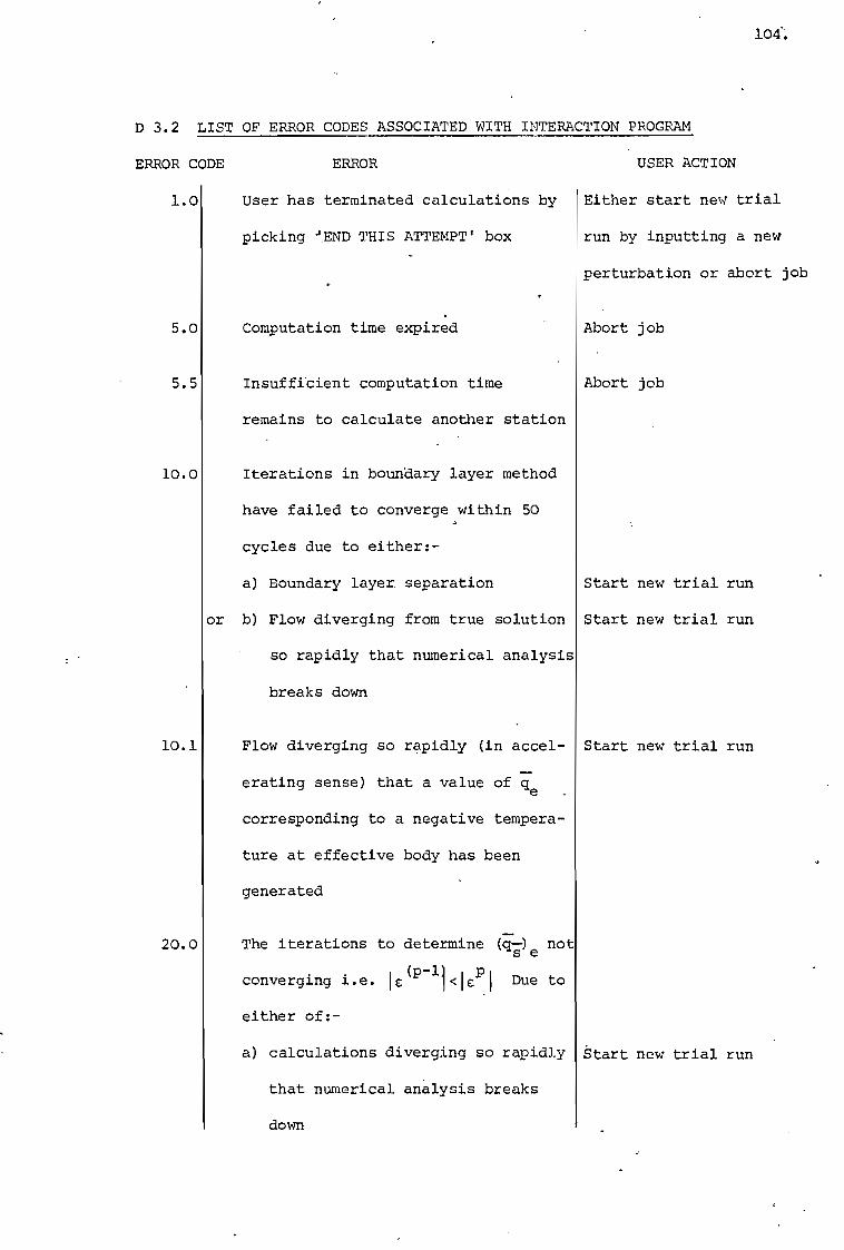
104.
D 3.2 LIST OF ERROR CODES ASSOCIATED WITH INTERACTION PROGRAM
ERROR CODE ERROR
User has terminated calculations by
picking 'END THIS ATTEMPT' box
Computation time expired
Insufficient computation time
remains to calculate another station
USER ACTION
Either start new trial
run by inputting a new
perturbation or abort job
Abort job
Abort job
Start new trial run
Start new trial run
Start new trial run
Start new trial run
Iterations in boundary layer method
have failed to converge within 50
cycles due to either:-
a) Boundary layer separation
or b) Flow diverging from true solution
so rapidly that numerical analysis
breaks down
Flow diverging so rapidly (in accel-
erating sense) that a value of cae
corresponding to a negative tempera-
ture at effective body has been
generated
The iterations to determine (q--s)e not
converging i.e. Ic(p-11<lei Due to
either of:-
a) calculations diverging so rapidly
that numerical analysis breaks
down
1.0
5.0
5.5
10.0
10.1
20.0
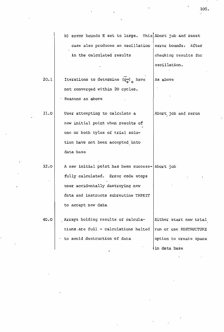
105.
b) error bounds E set to large. This Abort job and reset
case also produces an oscillation error bounds, after
in the calculated results checking results for
oscillation.
Iterations to determine (q--s)e have
not converged within 20 cycles.
- Reasons as above
User attempting to calculate a
new initial point when results of
one or both tyles of trial solu-
tion have not been accepted into
data base
As above
Abort job and rerun
A new initial point has been success- Abort job
fully calculated. Error code stops
user accidentally destroying new
data and instructs subroutine TAPEIT
to accept new data
Arrays holding results of calcula- Either start new trial .
tions-are full - calculations halted run or use RESTRUCTURE
- to avoid destruction of data option to create space
in data base
20.1
31.0
32.0
40.0
106.
'REFERENCES
Bertram, M.H. 1954
Blottner, N. 1964
Brown, S.N. and 1969
Stewartson, K.
Buckmaster, J. 1970
-
Cheng, H.K. et al 1961
Christian et al 1970
Viscous and leading edge thickness effects
on the pressure on the surface of a flat
plate in hypersonic flow.
J. Aero. Sci. 21, pp.430-431.
Non-equilibrium laminar boundary layer flow
for ionised air.
AIAA Jnl. 2, 11, pp.1921-1927.
Laminar Separation.
Annual Review of Fluid Mechanics pp.45-72.
Annual Reviews Inc., Palo Alto, California.
The behaviour of a laminar compressible boun-
dary layer on a cold wall near a point of
zero skin friction.
J. Fluid Mech. 44, part 2, pp.237-247.
Boundary layer displacement and leading edge
bluntness effects in high-temperature hyper-
sonic flow.
J. Aero. Sci. 28, p.353.
Similar solutions of the attached and separated
compressible laminar boundary layer with heat
transfer and pressure gradient.
ARL 70-0023.
107.
Control Data Corpn. 1970 Interactive graphics system, 6000 series,
version 1.
Publication no. 44616800.
Control Data Corpn. 1971 Scdpe reference manual, 6000 series,
version 3.3.
Publication no. 60305200.
Cox, R.N. and 1965 Elements of hypersonic aerodynamics.
Crabtree, L.F. The English Universities Press Ltd.
van Dyke, M.
Fitzhugh, H.A.
Fox, L.
1969 Higher order boundary layer theory.
Annual Review of Fluid Mechanics, pp.265-292.
Annual Reviews Inc., Palo Alto, California.
1969 Numerical studies of the laminar boundary
layer equations for Mach numbers up to 15.
J. Fluid Mech. 36, part 2, p.347.
1957 The numerical solution of two point boundary
value problems in ordinary differential
equations.
Clarendon Press.
Gadd, G.E. 1957 ARC CP no.331.
Garvine, R.W. 1968 Upstream influence in viscous interaction
problems
Physics of Fluids 11, 7, pp.1413-1423.

Georgeff, M.P.
Georgeff, M.P.
108.
1972a A comparison of integral methods for the
prediction of the laminar boundary layer-
shock interaction.
I.C. Aero Report 72-01.
1972b An extension of the Lees-Reeves-Klineberg
method to two and three dimensional boundary
layers with arbitrary wall cooling ratio.
I.C. Aero. Report 72-02.
Holden, M.S. 1971
Howarth, L. • 1938.
von Karman Inst.
for Fluid Mech.
1972
Klineberg, J.M. 1968
Lees, L. 1956
Boundary layer displacement and leading edge
bluntness effects on attached and separated
laminar boundary layers in a compression
corner. Part 2; experimental study.
AIAA Jnl 9, pp.84-93.
On the solution of the laminar boundary layer
equations.
Proc. Roy. Soc. A 164.
Notes for lecture series 44.
Theory of laminar viscous-inviscid interaction
in supersonic flows.
Ph.D. Thesis, Graduate Aeronautical Labs.,
California Institute of Technology.
Influence of the leading edge shock wave on
the laminar boundary layer at hypersonic speeds.
J. Aero. Sci., 23, pp.594-600.
109.
Leigh, D.C.F. 1955 The laminar boundary layer equations; a
method of solution by means of an automatic
computer.
Proc. Comb. Phil. Soc. 51, p.320
Mohammadian, S. 1970 Hypersonic Boundary Layers in Strong
Pressure Gradients:
Ph.D. Thesis, University of London.
NACA 1953 Equations, tables and charts for compressible
flow.
Technical report 1135.
Sells, C.C.L. 1966 Two dimensional laminar boundary layer
programme for a perfect gas.
R and M no.3533.
Smith, A.M.O., and ' 1963 Solution of Prandtl's boundary layer equations,
Clutter, P.W. Douglas Aircraft Engineering paper 1530.
Spalding and 1967 Heat and Mass transfer in Boundary Layers.
Patankar Morgan-Grampian.
Stewartson, K. 1949 Correlated incompressible and compressible
boundary layers.
Proc. Roy. Soc. A200 p.84.
Stewartson, K. 1964 The theory of laminar boundary layers in
compressible flow.
Oxford Mathematical Monographs.
110.
Stollery, J.L. 1970 Hypersonic viscous interaction on curved
surfaces.
J. Fluid Mech. 43, part 3, pp.497-511.
Stollery, J.L. 1971 Hypersonic viscous interaction.
Fluid Dynamics Trans. 6, part 2, pp.545-562.
Wornom, S.F. and
1972 "Displacement Interaction and Surface Curvature Werle, M.J.
Effects on Hypersonic Boundary Layers"
AIAA 10th. Aerospace Science Meeting paper.

FIGURES AND TABLES
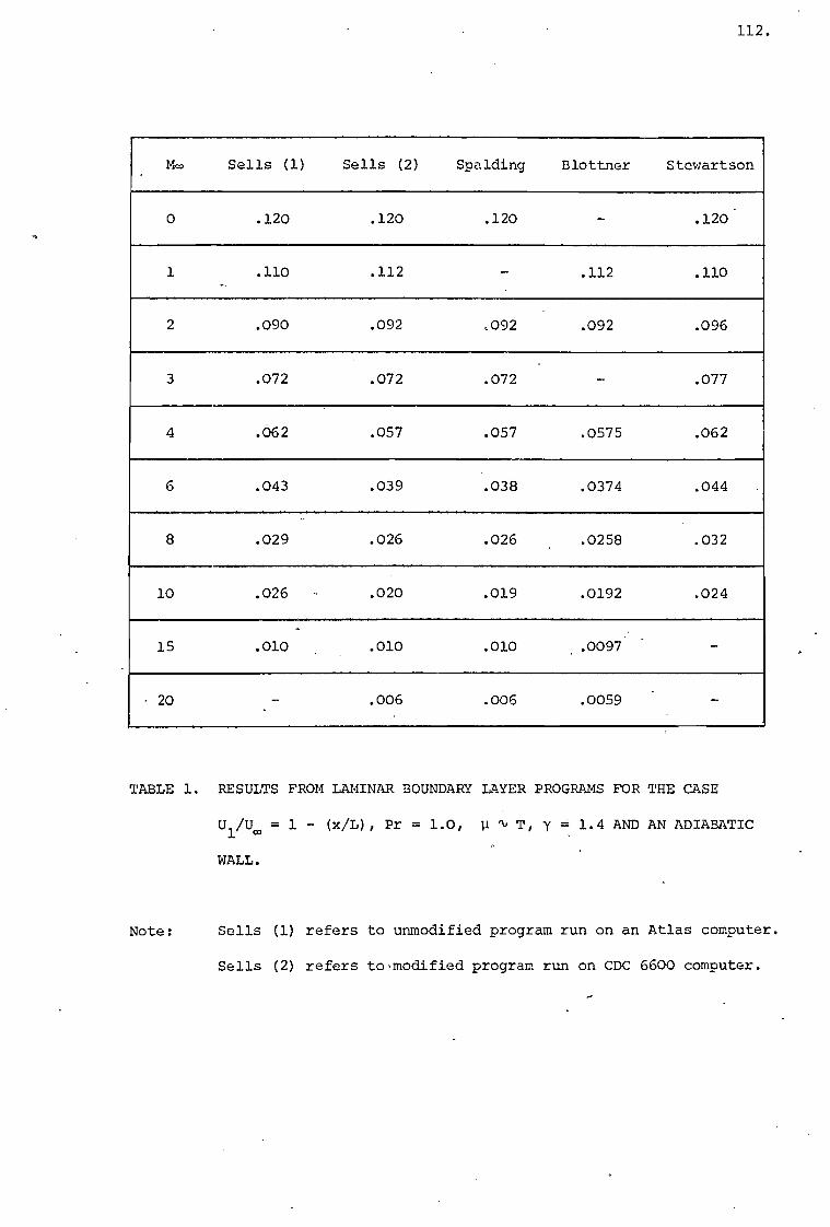
112.
1403 Sells (1) Sells (2) Spalding Blottner Stewartson
0 .120 .120 .120 - .120
1 .110 .112 - .112 .110
2 .090 .092 .092 .092 .096
3 .072 .072 .072 - .077
4 .062 .057 .057 .0575 .062
6 .043 .039 .038 .0374 .044
8 .029 .026 .026 .0258 .032
10 .026 .020 .019 .0192 .024
15 .010 .010 .010 .0097 " -
- 20 - .006 .006 .0059 -
TABLE 1. RESULTS FROM LAMINAR BOUNDARY LAYER PROGRAMS FOR THE CASE
U1 /Uco = 1 - (x/L), Pr = 1.0, p ti T, y = 1.4 AND AN ADIABATIC
WALL.
Note: Sells (1) refers to unmodified program run on an Atlas computer.
Sells (2) refers to-modified program run on CDC 6600 computer.
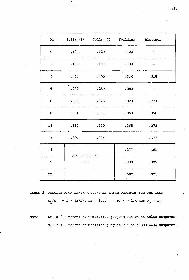
113..
M. Sells (1) Sells (2) Spalding Blottner
0 ,120 .120 .120 -
2 .139 .138 .139 -
4 .206 .205 .204 .208
6 .282 .280 .282 -
8 .324 .326 .328 .333
10 .351 .351 .353 .358
12 .365 .370 .368 .373
13 .380 .384 - .377
14
METHOD BREAKS
DOWN
.377 .381
15 . .380 .385
20 .390 .391
TABLE 2 RESULTS FROM LAMINAR BOUNDARY LAYER PROGRAMS FOR THE CASE
U1/Uco - 1 - (x/L), Pr = 1.0, 11 a T, y = 1.4 AND Tw = Tom.
Note: Sells (1) refers to unmodified program run on an Atlas computer.
Sells (2) refers to modified program run on a CDC 6600 computer.
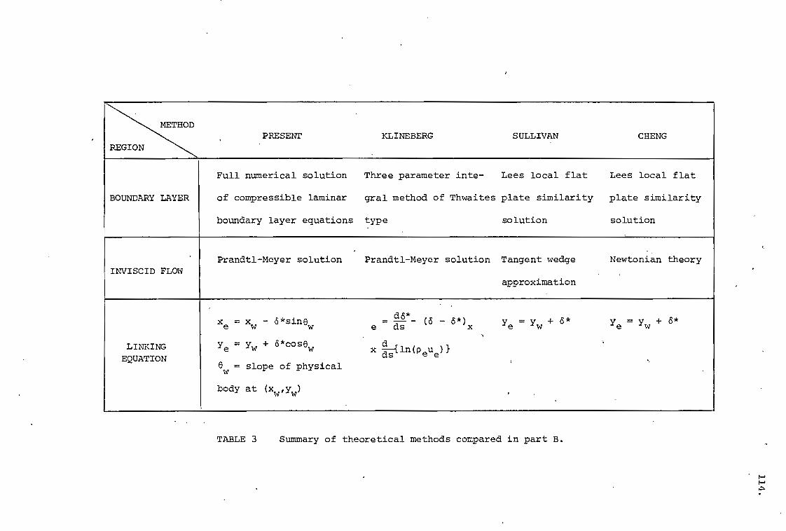
METHOD PRESENT
REGION KLINEBERG SULLIVAN CHENG
BOUNDARY LAYER
Full numerical solution
of compressible laminar
boundary layer equations
Three parameter inte- Lees local flat
gral method of Thwaites plate similarity
type solution
Lees local flat
plate similarity
solution
INVISCID FLOW Prandtl-Meyer solution Prandtl-Meyer solution Tangent wedge
approximation
Newtonian theory
LINKING EQUATION
xe = xw - Pcsinew .
ye = yw + d*cosew
ew = slope of physical
body at (xw,yw)
- . d6* - (6 - 6*)
a = as- ds x
x ---(1n(peue)1 ds
Ye = Yw -I- 6*
,
Ye = Yw + 6*
.
TABLE 3 Summary of theoretical methods compared in part B.
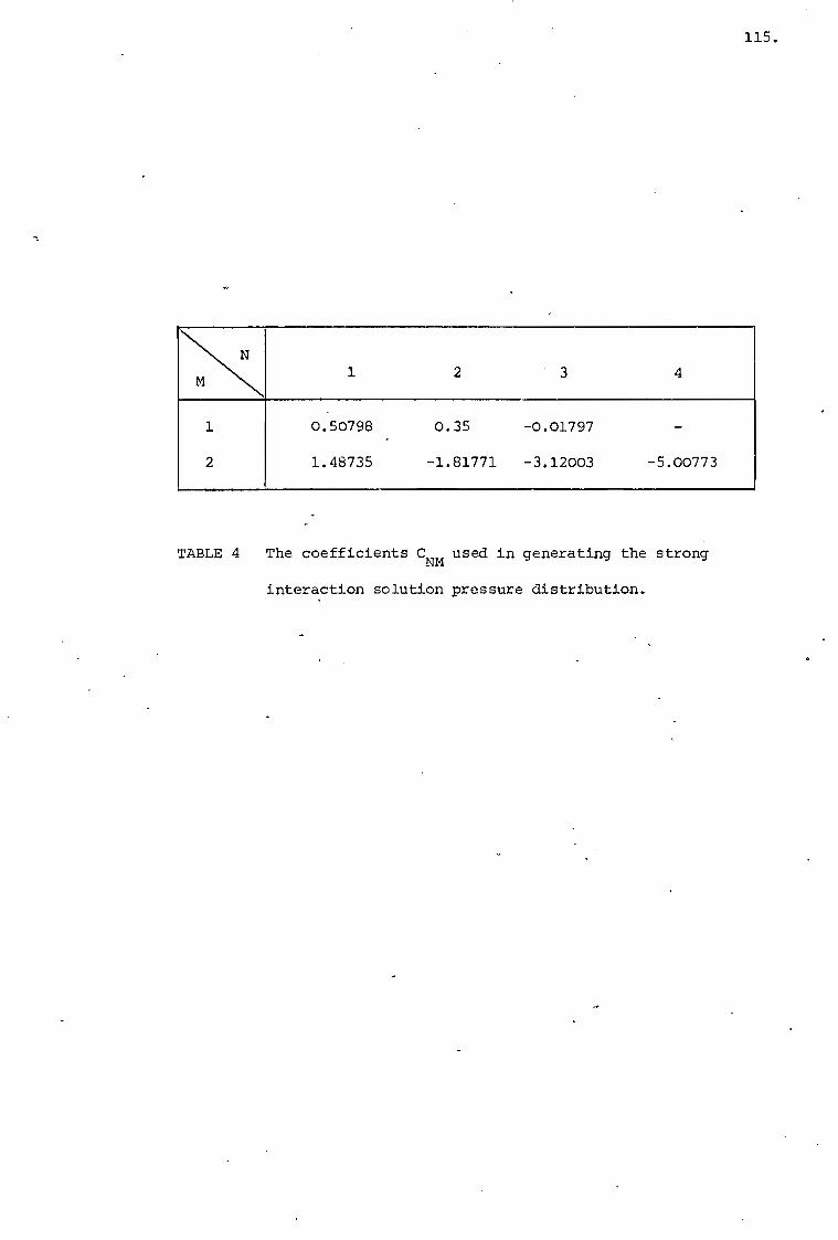
115.
N
M 1 2 3 4
1 0.50798 0.35 -0.01797 -
2 1.48735 -1.81771 -3.12003 -5.00773
TABLE 4 The coefficients CNM used in generating the strong
interaction solution pressure distribution.
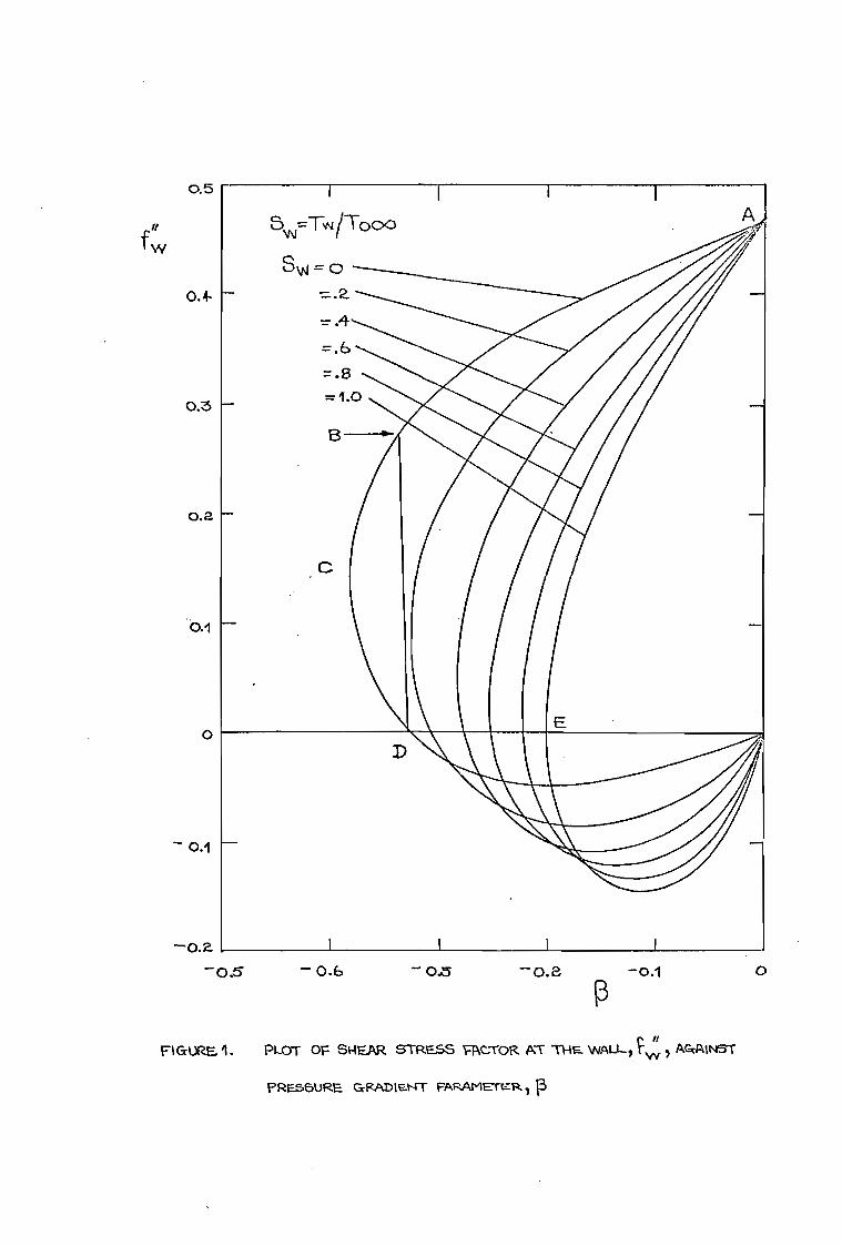
— 0.6 — 0.5 —0.2 —0.1 0
FIGURE. 1. PLOT OF SNEER STRESS FACTOR AT THE. WAU-. r\iv) AcwAINST
PREse•URE GRADIENT pARAmETKR = p
0.5
0.4
0.3
0.2
0.
- 0.1
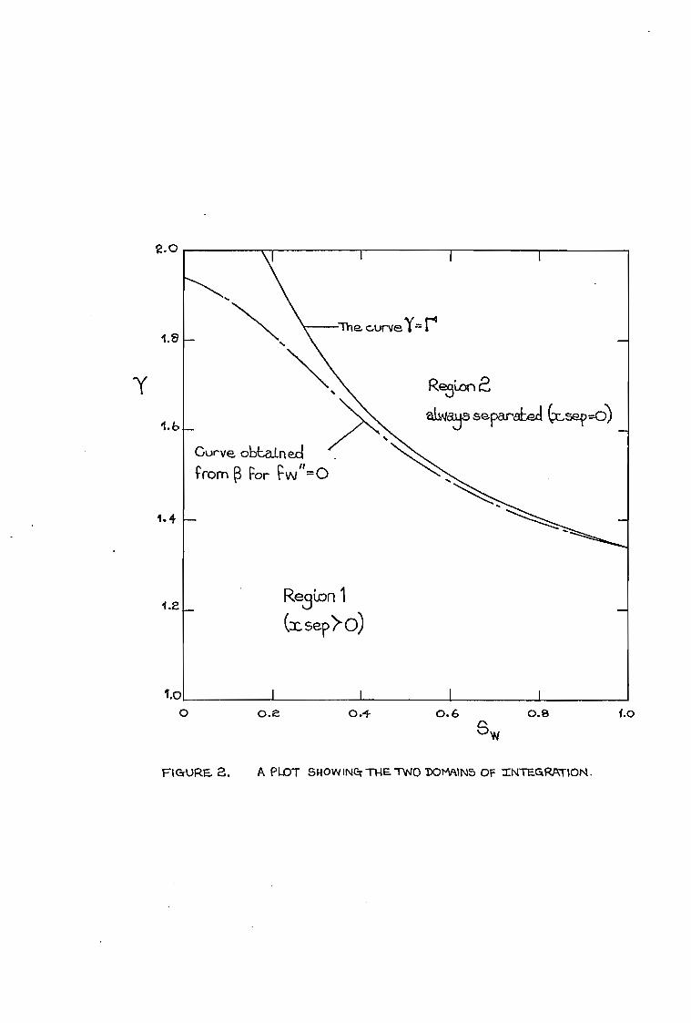
Re3Lon 1 (i sepo)
1.2 _
to
I
0 0.e 0.4 0.6 SW
0.9 1.0
FICTURE. 2. A PLOT SHOw INC; -11-1E TWO DOMAINS OF 'INTE.GRATION.
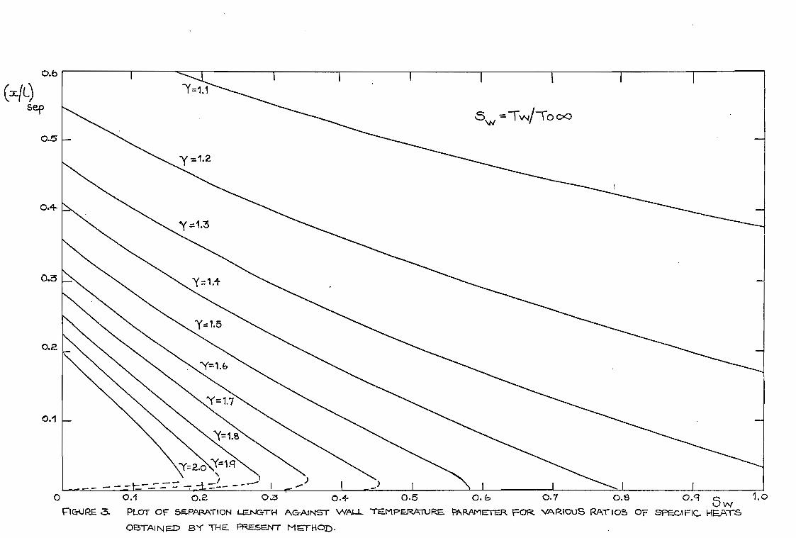
0.5--
0.4
0.3
0.2
0.1
I= 2.o Y'l-q
__....i- ••-• ...,
_- -_-:.-- - - -- o 0.1 0.2 0.3 0.4- 0.5 0.b 0.7 0.8 0.q1....,w 1.0
FIGURE Z. PLOT OF SEPARATION I-MN/GT-14 AG-AiNST WALL 'TEMPERATURE. PARAMETER FOR VARIOUS RAT 105 OF SPECIFIC HEATS OBTAINED BY THE PRESENT M M-14 op•
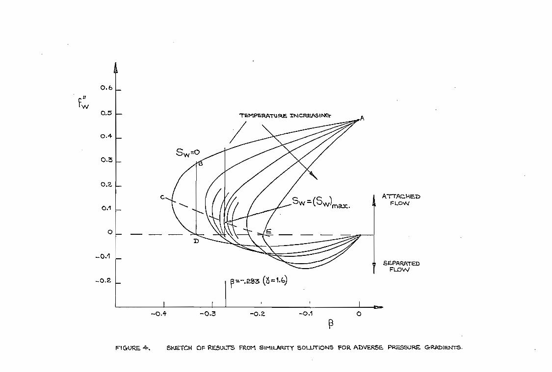
ATTAC-1-1E7) FLOW
0.6
0.5
0.4
0.3
0.2.
0.1
-0.1 SEPARATED
FLOW
=-22,3 (6=1.G)
-0.2
-0.2
0
R -0.4 -0.3
T2MPal4A-TUR.E, It3CREASINer
FIGURE 4. SKETCH OF RESULTS FROM SIMILARrrr SOLUTIONS FOR ADVERSE. PRESSURE GRADIENTS.
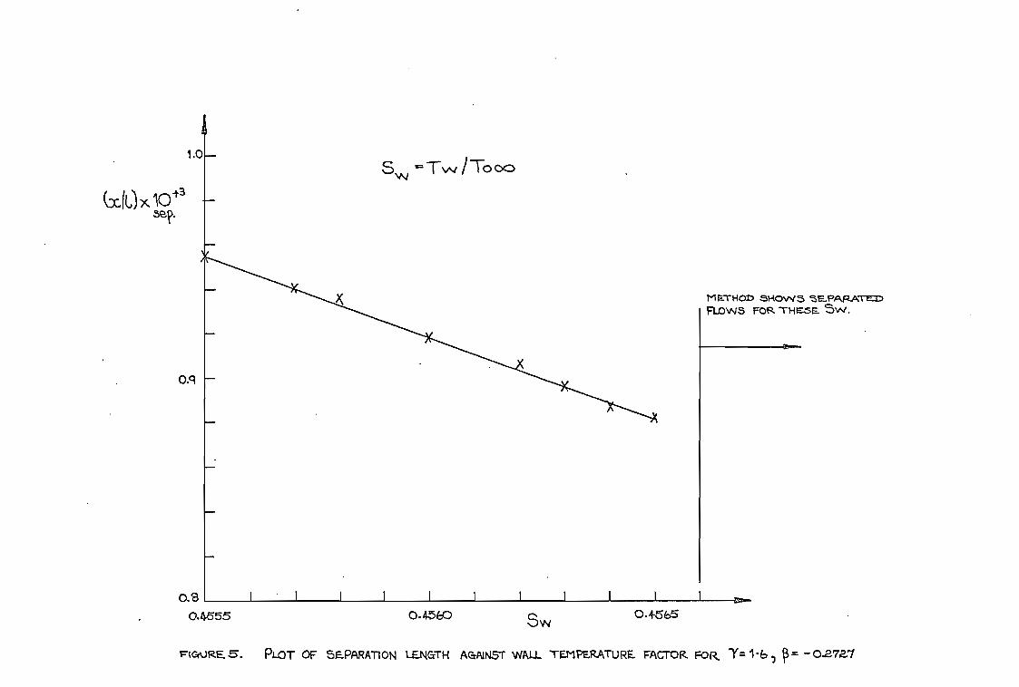
Sw =Tv.' /T000
U(c)x10-'3 ZS?.
0.8 I I I I I I I I I I 0.4555 0.4560
SW 0.4565
Ft x..)RE 5. PLOT OF SEPARATION LENGTH AGAINST WALL TEMPERATURE FACTOR FOR 1=1-61 13= -0272.7
1.0
MR.THOD sHow 3 SEPARATED FLOWS FOR THESE 3w.
0.9
=1-
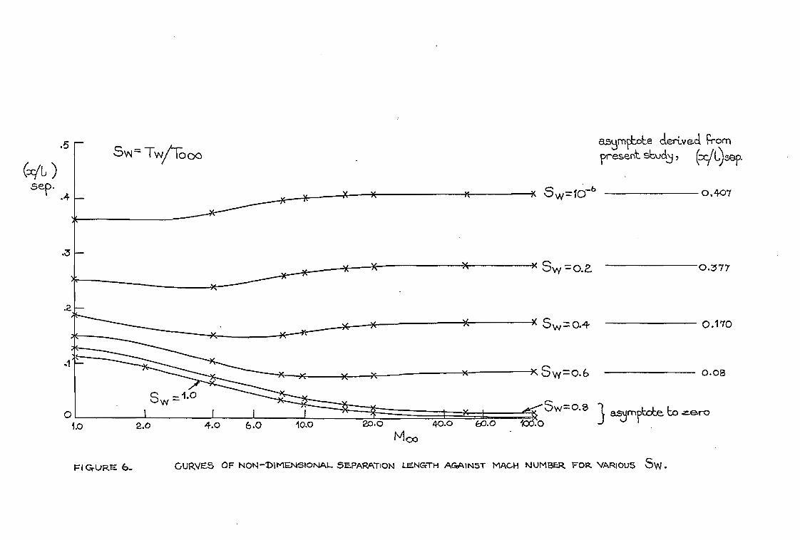
a.zrnFEoLe clerivect From ?resent sbudj , (Dif(,)sef.
0.407
0.7 7
0.110
5111r= TW/T-Poo
)(-----X Sw = 0.4
X----X >f-----X S w = O.6 0.08
1.0 2.0 4.0 6.0 10.0 20.0 40.0 60.0 S =..$ 3 asjrrfae E0 taro
MOO
FIGURE 6. GURVE5 OF NON-DIMENSIONAL. 5E.PARATiON LENGTH AGAINST MACH NUMBER FOR VARIOUS SW.
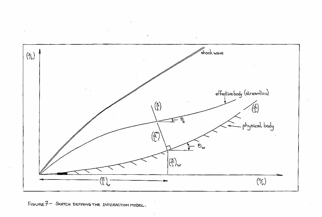
al111■111...
mock wave
eFFechve6ocla (streamline)
1) 4f)
......—__. pt-Ijsical. 6045
I Gi..) RE. 4— SKETCH 1) SS IN IN Ti-'...E. INTERACT{ ON MODEL- •
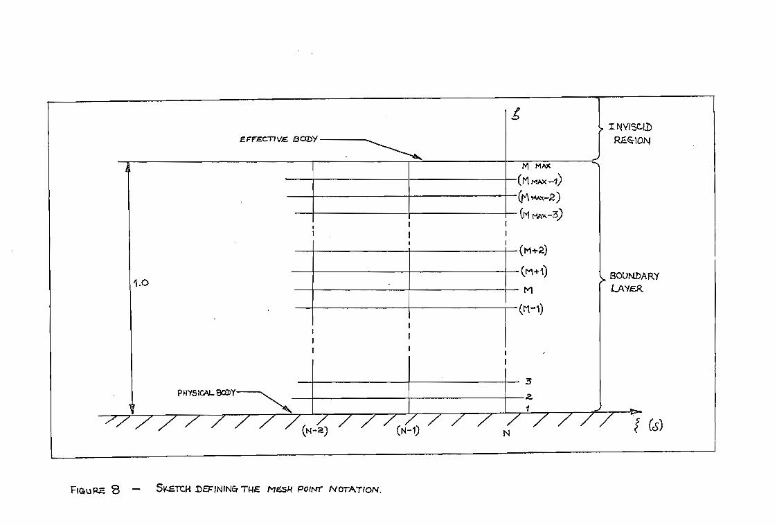
"NOLIA/1.0N 1Niod Hs3W 3H.L •NINI23(1
/ / / / a-N / )/ / /
N) / / /
NPN Java lvDISI.tid
(9) 1
O't
AWE/ 9A L.Loa ./3
AIIVeNCIOEI
NO1-V511 sJ I
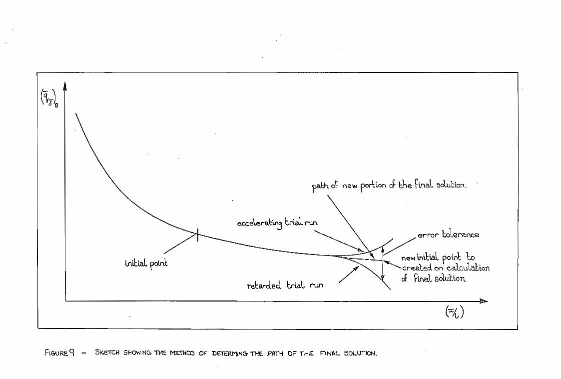
c new portion oc it e tinaL solution.
error tolerance
new initial_ Foin't ko created on cakdalion of Final sold:Lon.
'mit Foini,
regarded trial, run
ar_celeraku-5 trial. run
FiGuRECI - SKETCH SHOWING. METHOD OF DETERMINCT THE. PATH OF THE FINAL SOLUTCN.
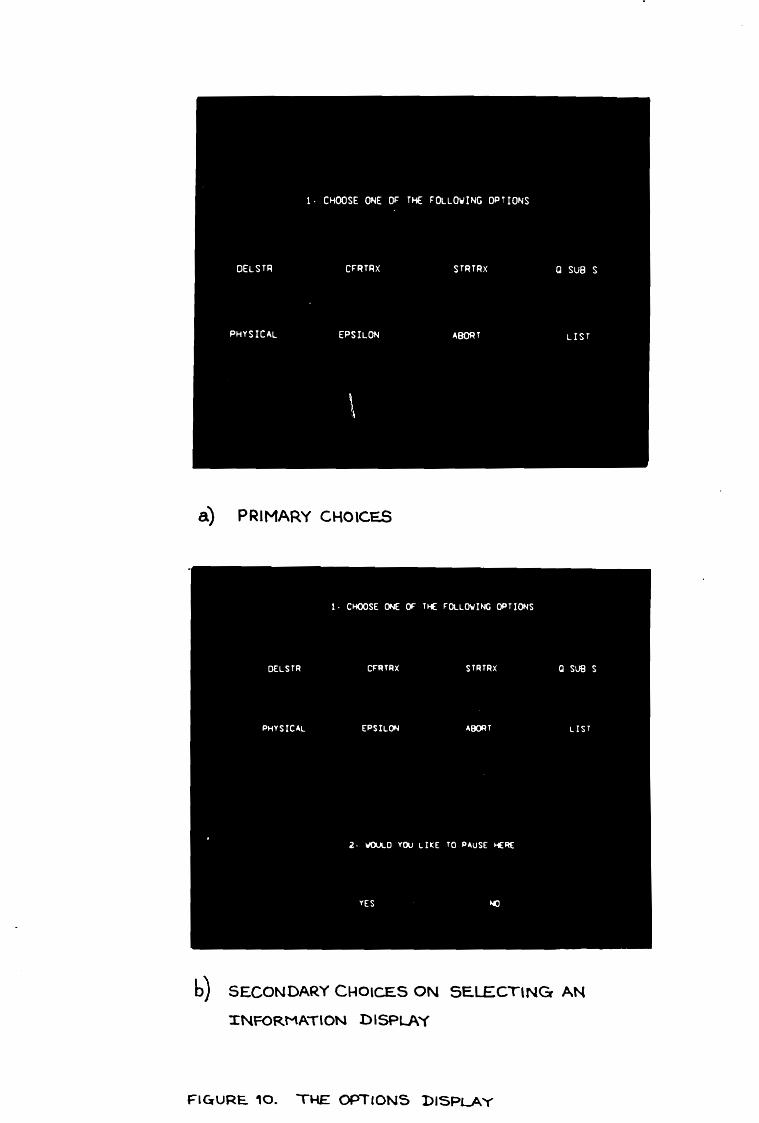
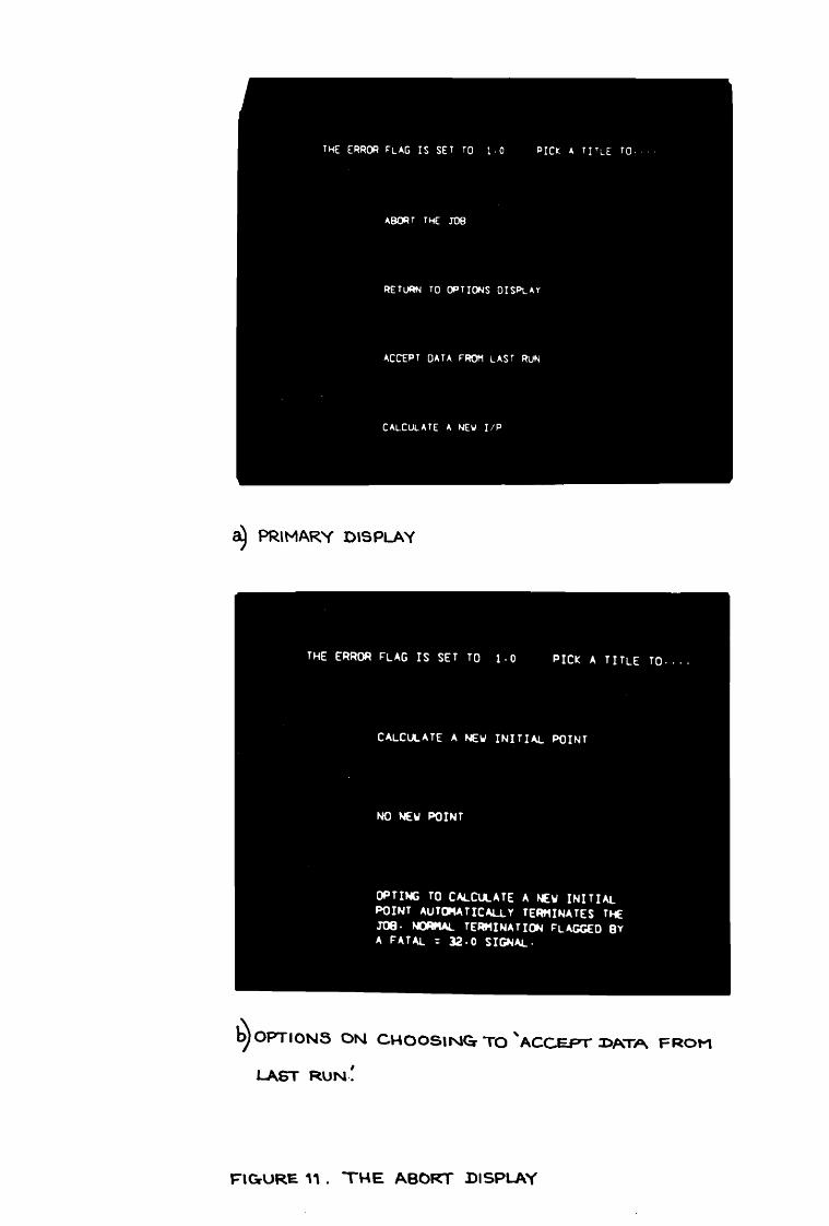
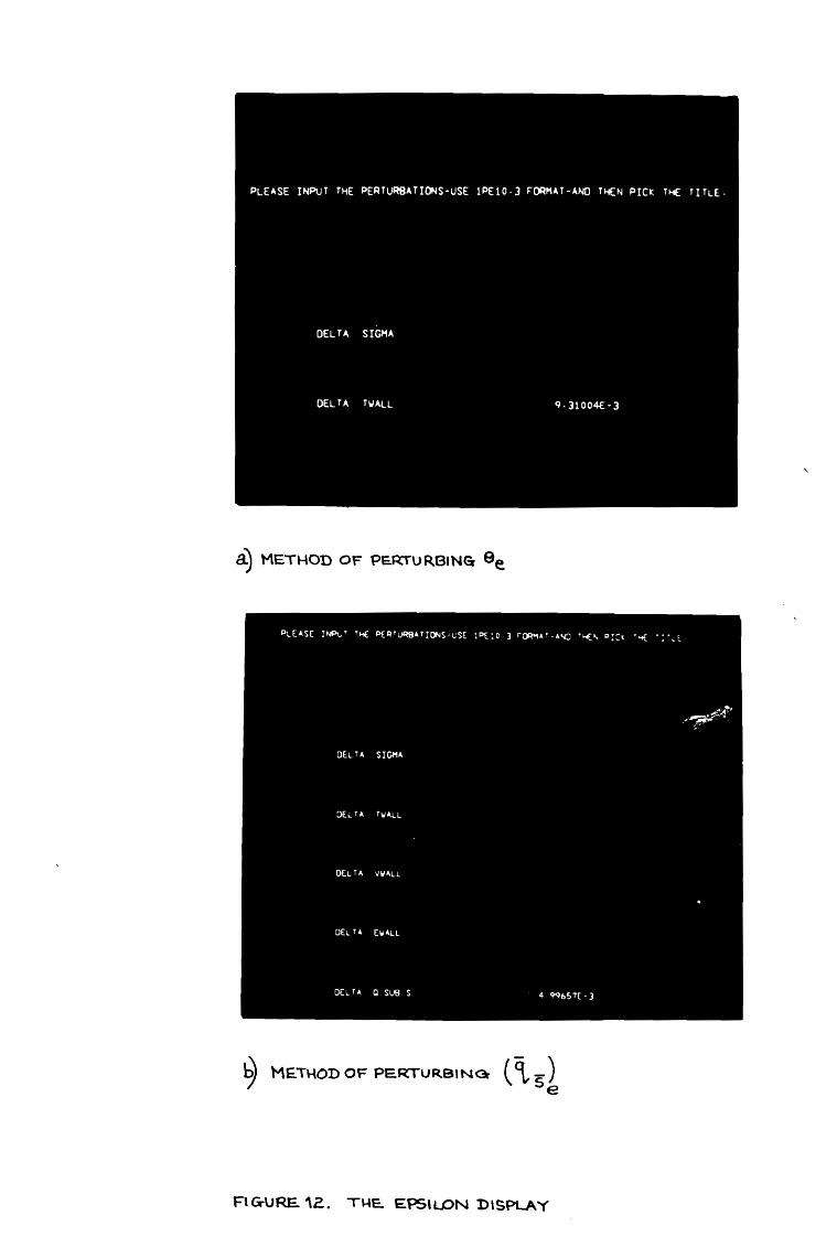
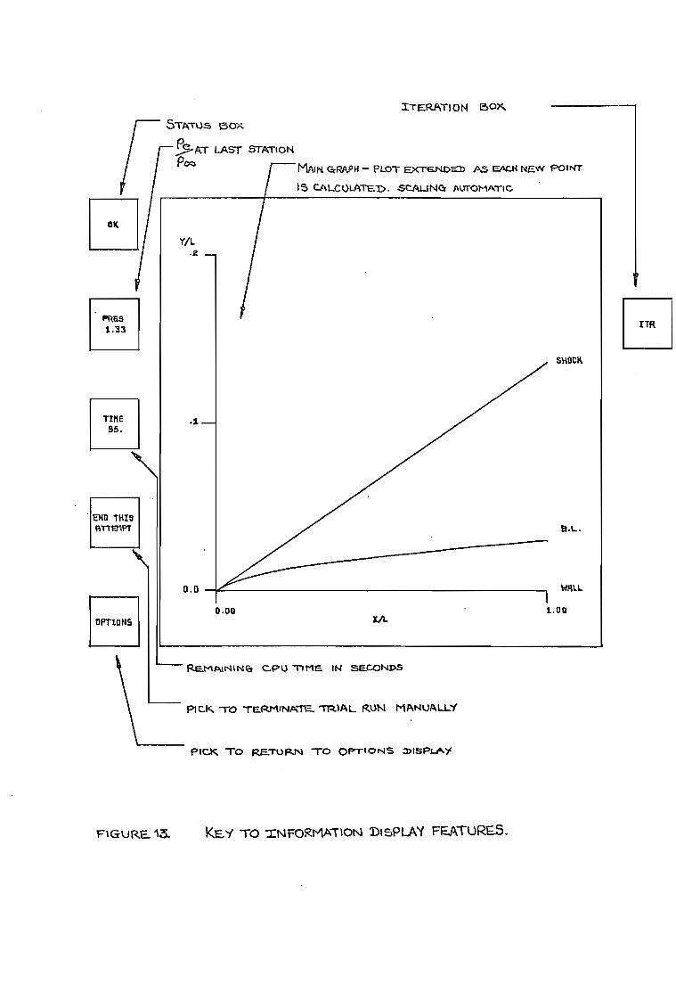
i/L .2
0.0
SHOOK
B.L.
WILL
0.00 1.00
Rat-INNINcIT GPU TIME IN SECONDS
DICK TO TERMINA-Te._ 1121AL RUN MANUALLY
PICK TO RaTURN TO OPTIONS amsPLAY
OK
TIME 95.
OPTIONS
ENO THIS fITTEMPT
I/L
PR Es 1.33
ITER/NT' ON 150,S r STATUS 150):
SAT LAST STATION Pc c, MAIN GRAPH — PLOT EXT,E.NOZ:1) AS EACH NEW POINT
15 CALCULATED. SCALING AUTOMATIC
TTR
FiGuRE.13. KEY TO INFORMATION DISPLAY FEATURE5.
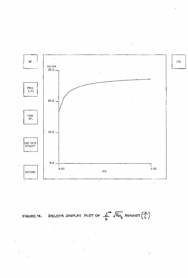
Oi■
DELSTR ?DX __
/TR
PPE3
1.'33
20.0_
TIME 87.
10.0
EN THIS fillEVET
0.0
0.00
OPTIONS
1 1.00
Ftaun..14. 1'ELSTR MISPLAY PLOT OF r14.---; AGAINST (t)
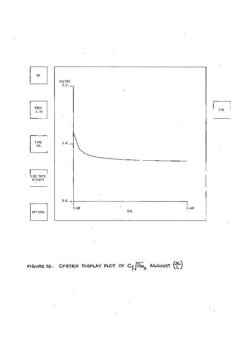
OK
CF1:TP.X 2.0 __
PRE0 1 .3'3
!IR
1111E: 05.
1 .1; ____
END 1H13 RTTEEPT
DC
0.00
X./1. .1.G0
FIGrURE. 15. C5 RTRX DISPLAY PUDT OF CFP;s AGrAil\151. e8
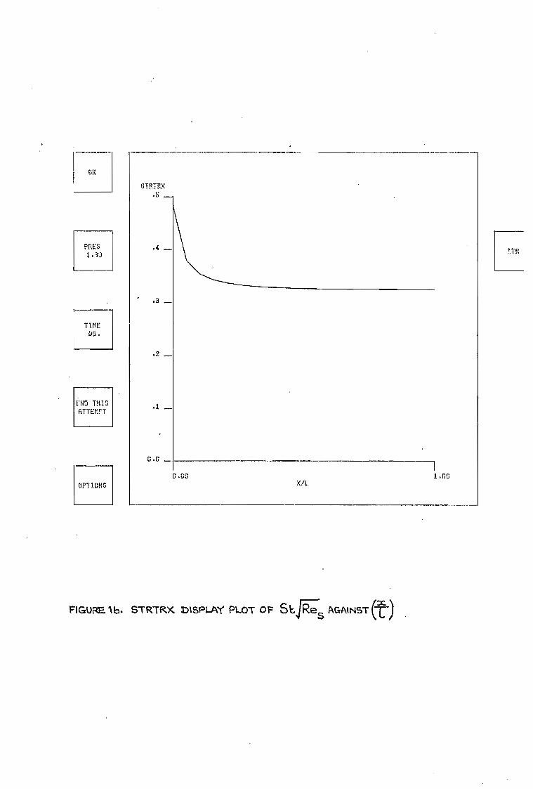
FIGURE. lb. STRTRX DISPLAY PLOT OF asifS AGAINST (t)
OPTIONS
(iTRTRX
.3
.2
O.0
C .00 I .00
.4 _ PRES 1.33
TIME 96 .
t:No THI3 RTTEM!'T
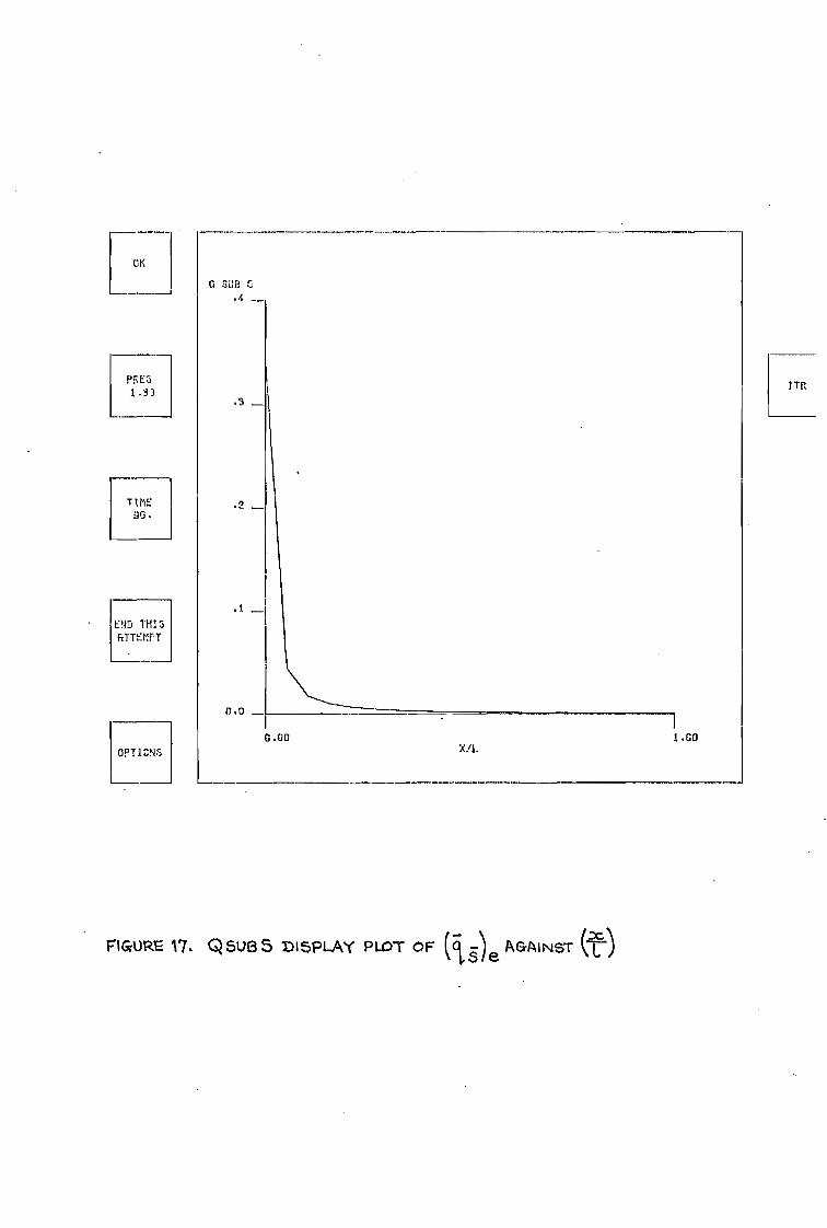
Cf<
ZUB C .4
.3
.2
0.0
1.80
1 .3 3 1Tft
TIME
END TH13 FiTTEMPT
OPT1CNS
FiGrURE 17. Q SOB S DISPLAY PLOT OF f
se AGAINST en
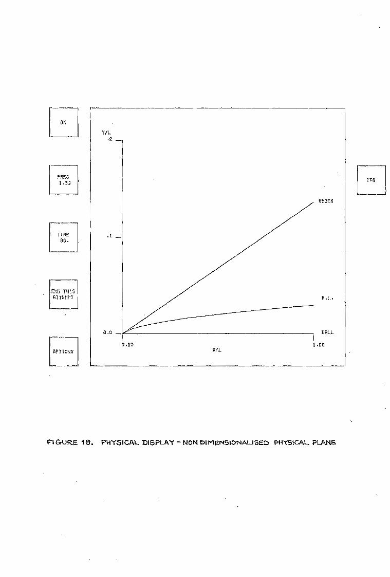
01'T 1CNG
END 1.11S RTTEITT
1 1ME .9G.
OK
PRE3 1.3]
Y/1. .2
Xfl.
0 .0
0.G0 1
SHOCK
NAIL.
GORE 18. PHYSICAL DISPLAY - NON otmeNsioNAu Sat:. PHYSICAL. PLANE.
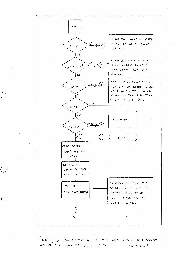
pri FoR Uri DscKtn4 tri (1 0-111 ot-1
czwel,t-rE-K n
Assocl c)r)C -
1-1-us 15 Lor.oCr) grro TE'E
vnelezi,e- Loci
111 F L-11 C-
FriTIIL>io
rlo
'TYPE
Er IA,
rrr pc I Stc,IALS r:::t,rv.P.1.qCNcr or
c Lk.,1-1.,rt ITT IvE4. rrivrptv - L!rCr,fc.
FIcrwrIoN 1??,!! LA`I'S .
C/CiriP!-$ CrICLET/,:t) of rzr.,177 or,1
C: i — F1 oY CoX .
ItviriTtLisE
11 NON ecru vr3Lt4E;
bit 14 ci SES nrr ItrrtrolfT6
Z-z;f3 Pe)v,r, I.
vnt. RE or vtlCunr ,„
FrIT/aL s )c, t4 r LS 1,44 C P3
STATC:- - iv To litior'r Y
5Gr;t P LO
DIart.avr Fir.sT Pin
or ornot/S. ourw,y
arTioti To GC riciccc,,
[—Nue(' 10 -) cuiv?-i- or )1! 1 C1A 1 ,̀'C'.3 TIM 4;1;70) e'r
&PArNics DrS rinY cot.; se:LC — nr, uro)
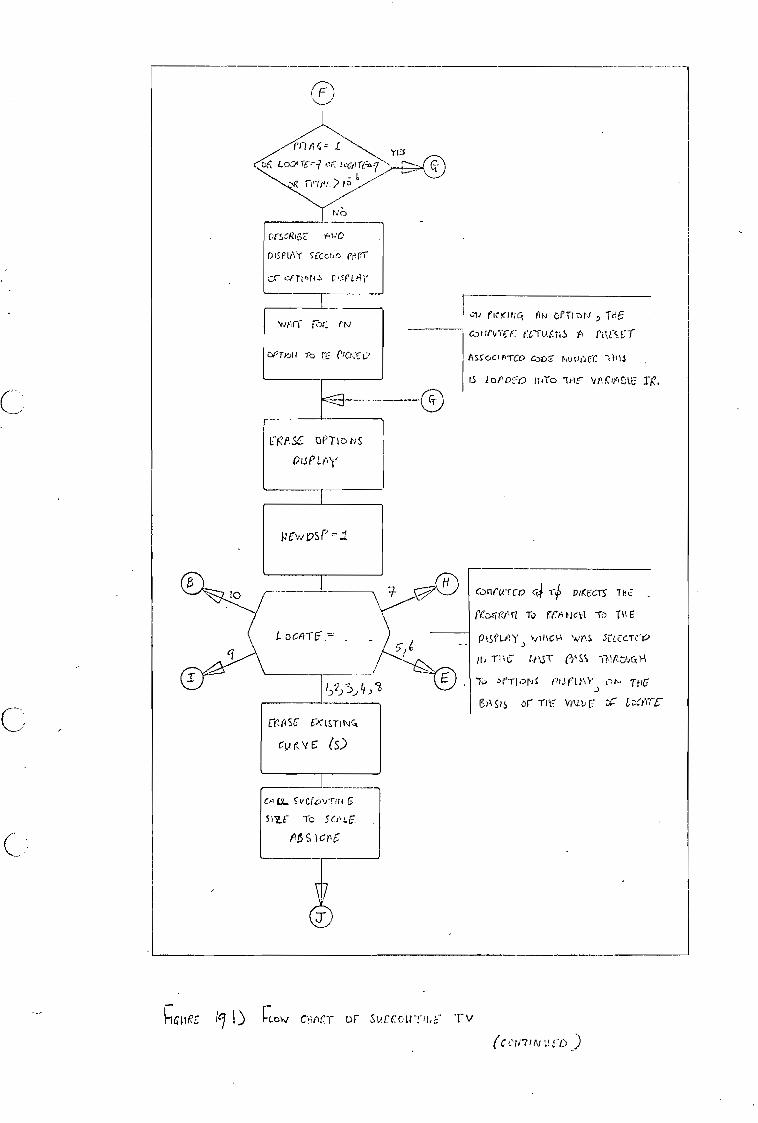
conewrco 4 r vIKE:crs the
ft.'41rzi41-1 To re,; Nett -to TN E
P iSf Lf-11" VII1C1-; `4./r.S 5(71, -crc:K,
T1,C 1-1\51- wss
zq'TIoNS 01.3r1:\ oni T.< IBA or Trff vim., 5 N.-- t DCKFC
10
1,2)3}
W1-111- (ti
U'rlorl Tc Cr CIC.Krc?
V.K PSC T S PisPLioC
fltiK11,16, 111.4 orT:-,m1 , THE
cot-leo-CF: t;cTottB fl riv,- 1.7i-
nssocip-rco 6305 rquorJa. Titls
IS Lopo,s--0 INT° 1HE- )1 OLE lg.
YES z-,f; Lo,..:11-t7-;? or L47,4r6;.7 rp-rpt.} 1; h
rfo prsflofs E
DISPLAY SCccr,r) rer
c P.sr LOY
a:1'1SC 0:1STINC1
CV E (s)
Cit0J -Nt4 5 5)E To
05S ICP5
{-7KneE lq t) C';PCT 01 SLIT Tv !cCt17!N
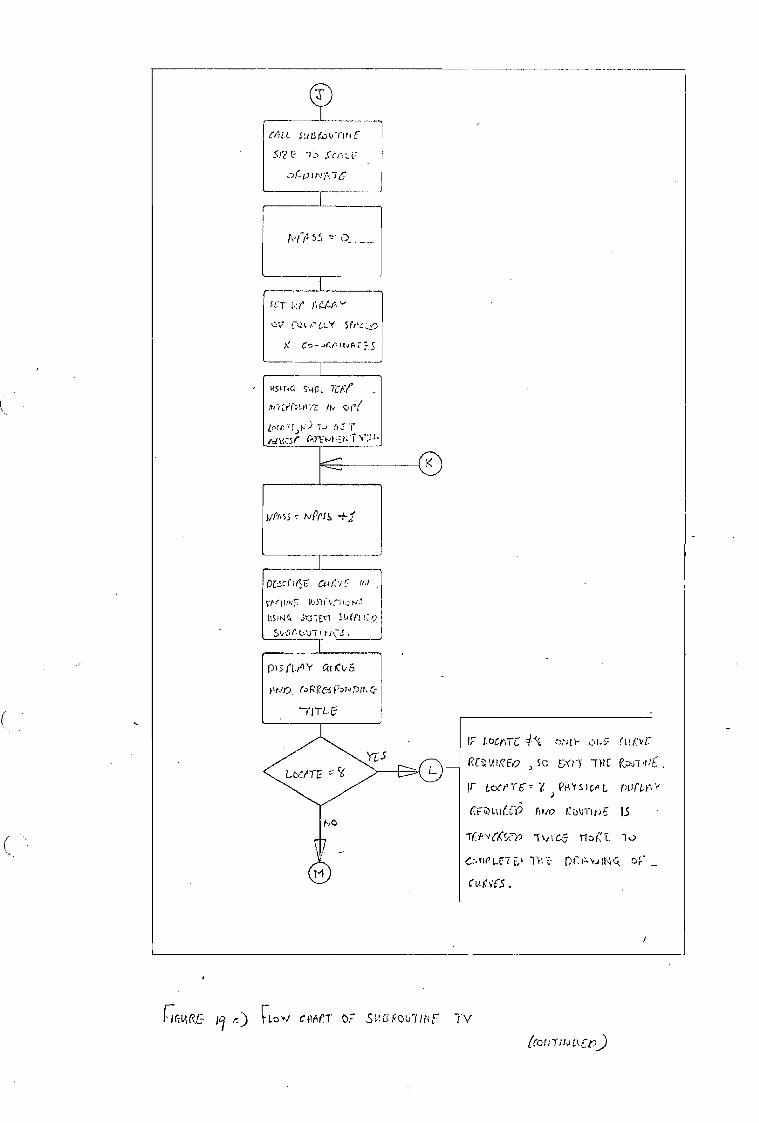
5,7
tv 11-1 5 5
5 CT 1,-:(
c L'e str,c,L.0
C '''t„-
511C SLI(L 71;fif° /ti
tpc 71, VL (41,:•:5r. Ps'Et-t,10-
0615 N POS
Dr,sc 9,)
vretoiF Mir) -SY...V7E11 St/ (f L ,.:7)
Stell Z.,t.“ i'It7.5
Pis (L, ti.ts
rz.R Res ())7 (-t-
--rrri-E
LoCnIC 4:(( op tA"' (-:)14C;
RCOJPEO SO DTI'
LocrIT6- -• ) poysicAL
cLaf,-13 At,,y) rtAiTirJE IS
rl
t' L7 Ey TWE- o'er:
CL13.
No
rultARG- i ) CT SVGrou7itir Tv
tap ti r t7)
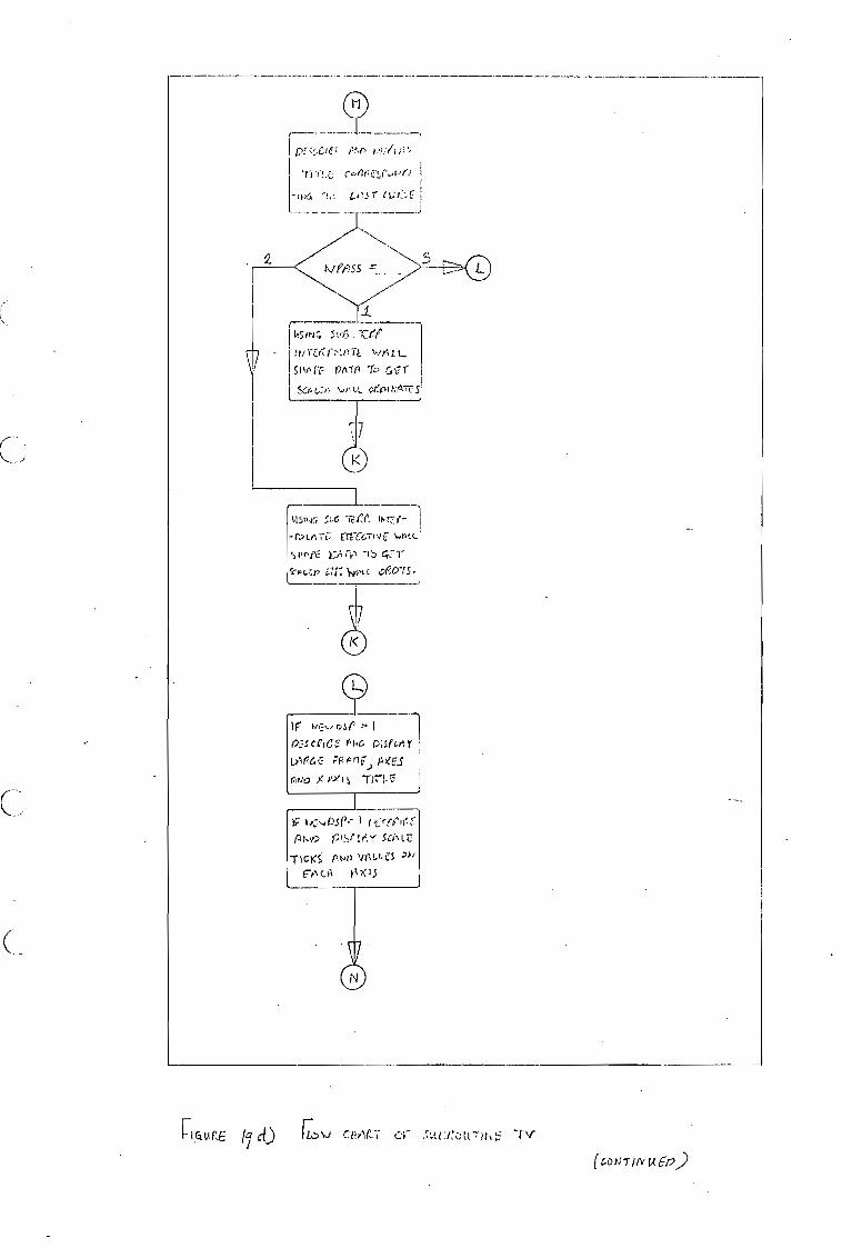
1 OL7Strie::' Pt■C PiStimr tilt76C: PRPelE.i ALES
Ptio x 'xl 'T)71. '15
rt:rtcrec PS(V.Y SMIZT
P.Nn VALueS .>+')
tA,SINe; .1,7fr
!&r: -1L
19A70 T7 G fl
C:ep)tiPsTE'S
7 r
-1 -r.)ircif--, nrccnvc ‘...Atr..
`It'PeC 174-1-r0 -1.. q.:.---r s-pi...-„n lit: }ont- oe075.,
f Tit,,c ccirot-q-? i
ri tAi',E d)
FLoN-1 or s...tixotrrn,t-F
(con17 Vrt-2)
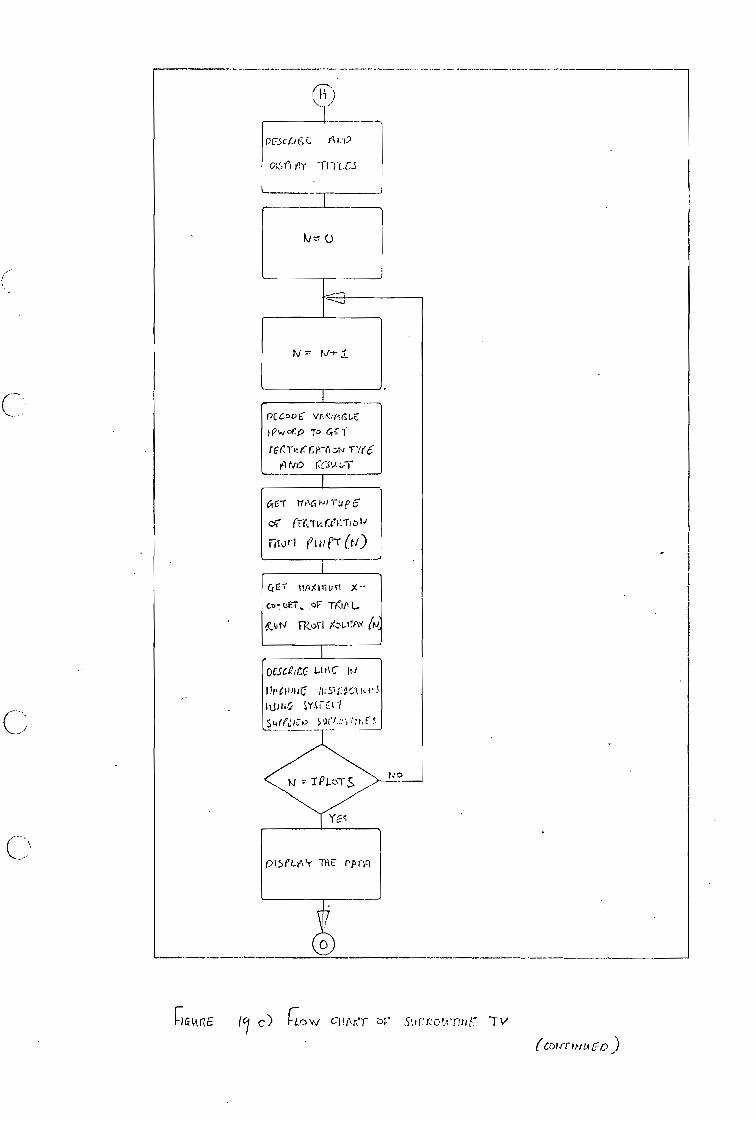
OCSCiet7 /Mt )0 Ilttell NC hjlti& Y&ii 5Liff/,.70
oisn yly 1-1
Li
PE CD viv<0 Pwogn TP 417 1'
re'ret -n.)tq No CC,s LT
arr 111A 1,11-up6
oc
Mori /21 (r4)
Ci tIPX 11 ol X - c. trr, oPTIP.L &tits TRal A:LAW
-ME" Pp-n=1
rialitruE 17 c) FLow crr,er b 3uci:c44.-ritir IV
(COIrrnvIA 6:0 )
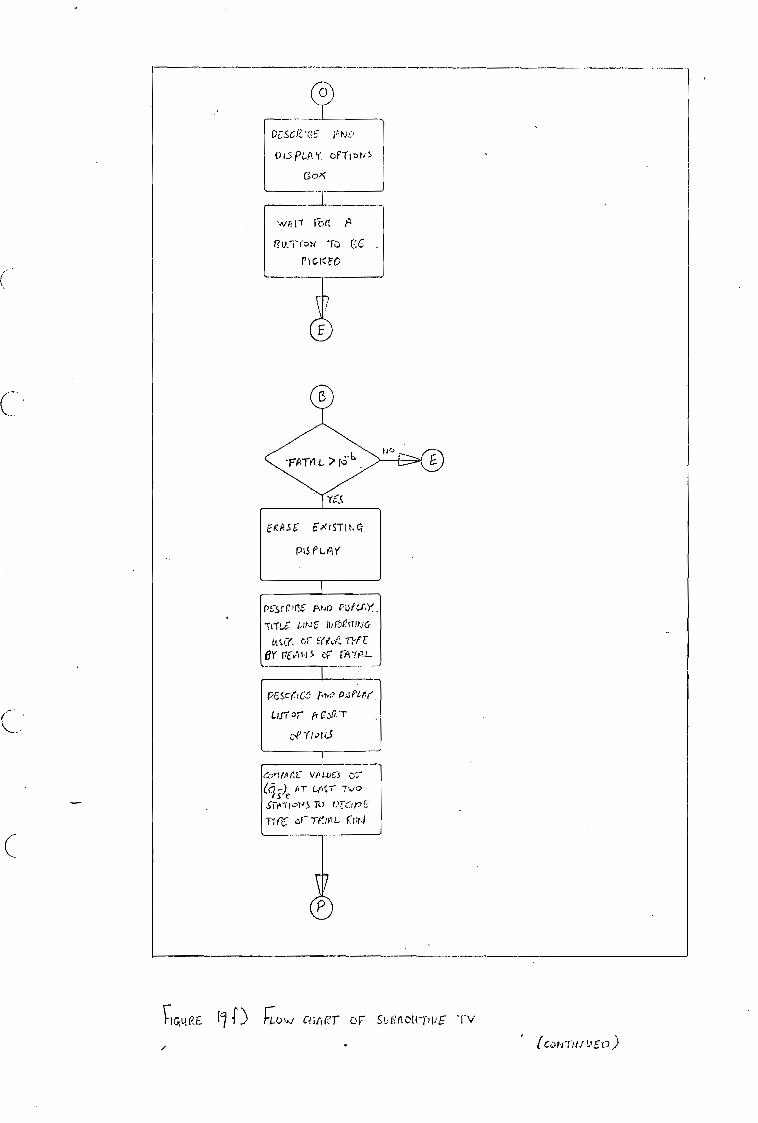
DC.SCk. I r3!-,' Otk
Li PLI1 Y. OPT! Dt; S
GoN
Wrr F.Nt A all,,-rat, TO CC
rICKFO
p5,-scria p,No
TITLE ItirOeflitj&
kcf.(. C &rid. -11f E BY rico-114s css: rtk'frt.t-
r pc,c-re.-, h r.? Dater Lis; or fr .
er...- ee,-)e AT Lt T Tvo
1.7.C.DE "WC or rvt.1
'1Gt t,),(ZE, f) Filow cdiArer OF Stietiott-ppE
rt"))
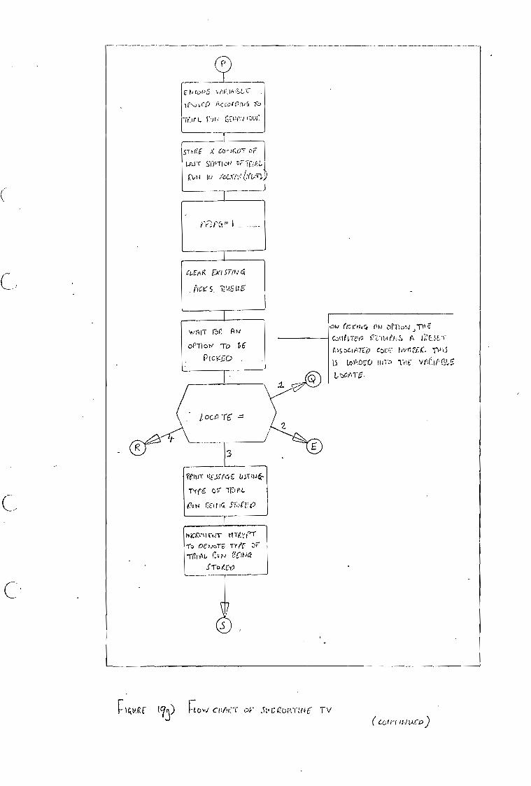
ENci,o5
i+ccocoiw; 7b
1
5-rprZE X. Co-r.)7 oF 1
1.-P,S1' .ST/ITIvi Dr iriPL
'\,,11 IN, A:;LX1‘,•,' 6(1.5r) 1
ct,rfkg Fxr sTIN 4
'inAC-.711C
ON ricroti allots) ,TtlE G711tV1Fr2 )7tsitierl.S A (:E.,!Ci" Ass ocIATEi9 fivrICTI% 1.5 1.0).1%.0 lilt TrI,E7
t,s1-11J4-.
rfr6 IDPL.
Alt+
NERvrivirr- VITE:(01. To 06■Jori: TYPE
{SUN 6CItsia Pro4C-19
FIcva[ (t) 1-tow cp/Vi 31t1;e0ATINC TV
(Cotrilti l,M.7())
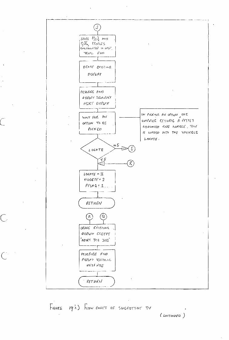
L
Eri cr-:" Eset .s7 )1,
P 1.50-S Y
1
WA a RA oPTIoPi Tz, GE
el CK
PESGe-ite r1 FIO
C IS FLOY Sa)rit),e-(Y
tA,(:;Lei- s(tit`(
O
Li:ET-Rat 3
ocra
CASE 67>eislitick
ourc-r■Y cx-cePT
"Aeto• TilE, aorf j r
PEScrir;6 oisrvy
116-ss
Kcrtiteri
ow PicKiw °Moil -ME
tfi 11 11 •(YES!' A 55 6 6:ATITV 63)."(7 N un G EC 1.'1l1 15 LoilL,Co INT0 71-kE VP0?161.-E
2-ocirTG
C
Flql4e G IC? flow C41/4:".-1 Or `.-,1,t/5 it4E: Tv,
totmworo )

Y(S
PC5ckteZ
J
r /PO
Tr TLC
ST\
ItS,71'; ), ',:vi!rt,ck'
3'.
,,\,,-;)!•1
MC PE-MA (r- Cr-no 14 15
In tv
c7 ri cr fiLiz
eart.7
PG• t n Ii
of s try vtr,- (-13ri -1111C- _
I 1.77•
1,! 6
17. Ca I S
r
LI 6.1w. -c• 17 ,2 Ii
cK
r)aucce 17 ) EIV/ ePtle:r 3r .1.;
)
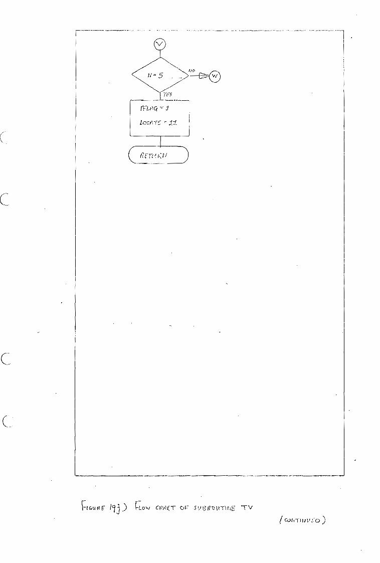
'11-75
rrtilk.-71
tocil -
1Cli FLOsed CPAkT CIF S 13 17 wt-1 r..iE TV
C01471111,t[o )

cse: is& 1,1,D IMS
-C2,6? E-No
iszx
1
prznaC
_ pisr1,117"
P On TS. r Min
015/1,1 re-r5
• a.%,'>\.
pcscricu Nvo
pi.fPielY MC
(Sax'
PE-sal/36' f ,No PIS -roly STA-NS_ 17,2x
pc- z.•.e.r.,:c7 0-P C — .
it'
YCs
firrie gtX
riov6 '77
riatvEt k FLcA, cpryl •.);" ..7:1 ".,(DUTME TV
( ec t47 1 tv ti et))
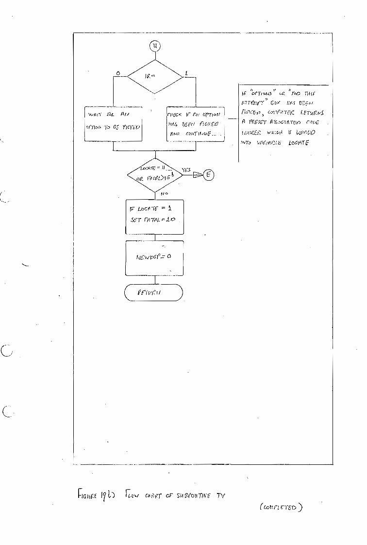
ernoi, _•lz, G; ricri:r2
mil' 1CGK lr At/
(1F,E7ti ncl(Fr9
pm). (01,7- 0.Jutf___
,r Loco I
Scr-T 1" -P Lc)
hirviPSr a
)F orr,nru Mo. 114 if p77-airy G r,(76:r.r
f , Cot TCK ilFTIACNS Fl ri:Escr A.)c-1 ri Tay) c
w G
INT.) c,TIT C
C errtfiri
Fleur 171) Ficv c,4,-)FT of shOrotiTKF TV
( Gott PI ETED
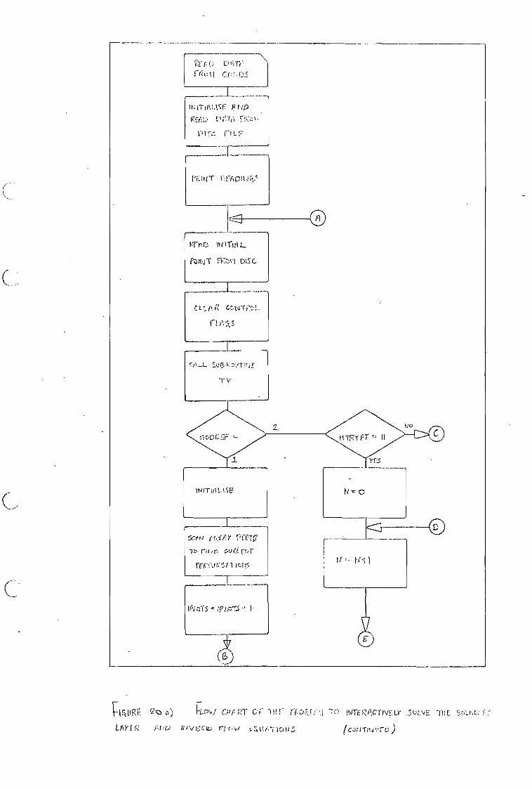
oDE SNE
ITIAL \SE N tiJ
CEt) t? ;1111 c.-1■••*'
Plc.": IILE
CLL Svf3
TV
f D 1%4IThIL
P\jT DI.,c
C L.r.
ri
1r4 iT LICE!
5c.pri PECI5
ovr.tnir
FEVP111 1=1"i_5
---\. C F t) Orr,
J
Fr ! Citt- ))<
C
11iRE Q FL-DV CFRY Cf -1F! (TD:i!,1.11 c it\ITEFACT/VE LY 3LvE
LAY 1'4 it) isciL y (, Lttv.y. 10 ti
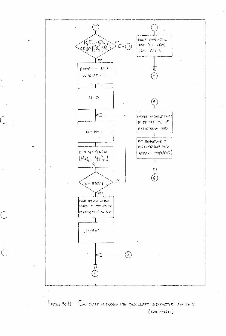
1\1--- 0
NO
YES
veltir ness6te: 1.1.51/4Q _
1Ji1ete cr STP.TIAL$
re PO.!o 1ito4,1.
rrioTT iv-1 NIVYPT I
177:1?- I
itiC01)E vACIAC,LE
P Tfrt arFo J 1
linGNIIPPr :c-
1 1v70
Atr.V/AY eiNCT(i11073)
Fillcr t)
FLOVCWT Cr 1Ott To CR/ C L 4TE ft.i Tri'fICTIV so.'1:T/Cti
( cot rr 11'4 )
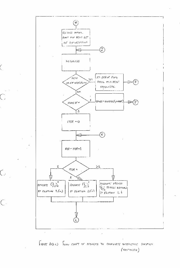
E.9
Itirritu-) E
-J
_ Pi? Im•.
ffr t1Y oveaFL0
3:71 r LriCi
ifkTp.L.
1-11r
QA{LI.S.- oLvOU(!imiktr..®
1 TEC "0
f Ct 1-14 r';1(7. itseirte
ibIKT Mir CIZI7;T GIST i
()r rr,17'er:1'11%ric
>2.
V
ITER rige+1
1.-1
..- ,... 1 , i
EST ITC (..1. ,i)c C.s-rcriATC r 1.- ),
Er rz,-z V.7) 1..1 2.5,0 IT Etifrnot4 2.51)
1
FLos, cHreT tr ricc,ciepTi to ci)Lcu Lfi1 b-s-rrr-F,L7 - 1\,,c sot trrIc,,t
(cotiTINivE b
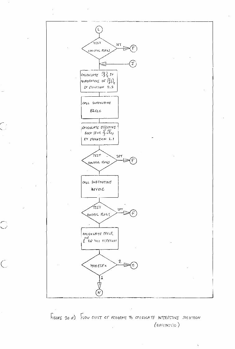
Cno_ StA$rov-riNtr-
INYCL.C.
onars°:. aros
cc14-1-AbL El FG05
cv 0,c
E . czp m‘.1 m./
ci
Col.Cv.LFTE" CI) Pr
q,,tporzp-71.11:17,or 110c
CY Crry-,00 2.3
CPLL StirRouTIN6
137.CLC.
et LC t.) P1-6 FE, boo- ;-rct1
rco,vivilot4 2. I
SET
FICI-11e6 r2Q d) riov C;rLT frO:iC);-11 Cr/cp.:P -1r CrnvFSc)l.tr-nr.w
(cortittiv:::))
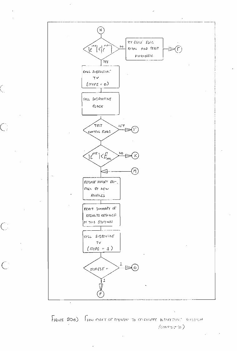
ST CO:a Fti.c,
Fn L t)ND fr INT
pr ,Ar:0511C
CALL. Sugibu'rit4r
"Tv
(rrYfr 0)
1
F.EplAcc iurrorY ho-
fllLc ar itoFILEL
FCINT SurintleY or
PSULTS CM' Cc;
fIT T;I I S
C
20C) FL 0\4 (.7!■ri."F 'to C L' yt ri y
A",er,,T■r; -1) )
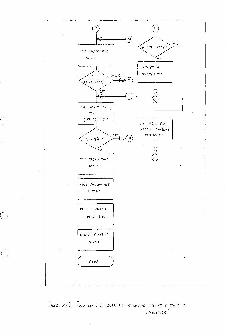
YE5 tiTOPT = aroet
1,10
riTgq1
viliCreT "t'
SIT of FtrAc,
FP-70 Eros DIPGric:11C.
CP 2. t Su f; r,o vTtrt E
ricTi4P,
PE,'7 C1-, CO, rilics
CO Vi
fp VT TETI-lit/A L
PlAquoSTIc
St r
1GLIPE 2C:(77) FLov CPrriT or r-, occeciit TO craccutffrc orTtErc-rriE
(collect-75'D
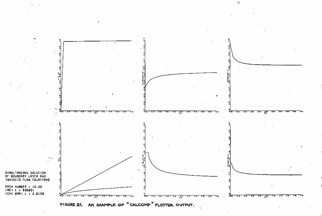
V WRE. 21. AN EXAMPLE, or ' cA.LcomP PLOTTER otrrpwr.
CIO i 11 •••• 1140 ear • • . •••• •••• • • •
4110 IN O W I. . I. ... . 1. •o ogo xn
I II CIO 1.0 91.. go co on
On.
SIMULTANEOUS SOLUTION OF BOUNDARY LAYER AND INVISCID FLOW EQUATIONS
MACH NUMBER = 12.25 IRE1 L = 835651 (CHI BAR) L = 2.0109
P.
s
eos • o e"
I
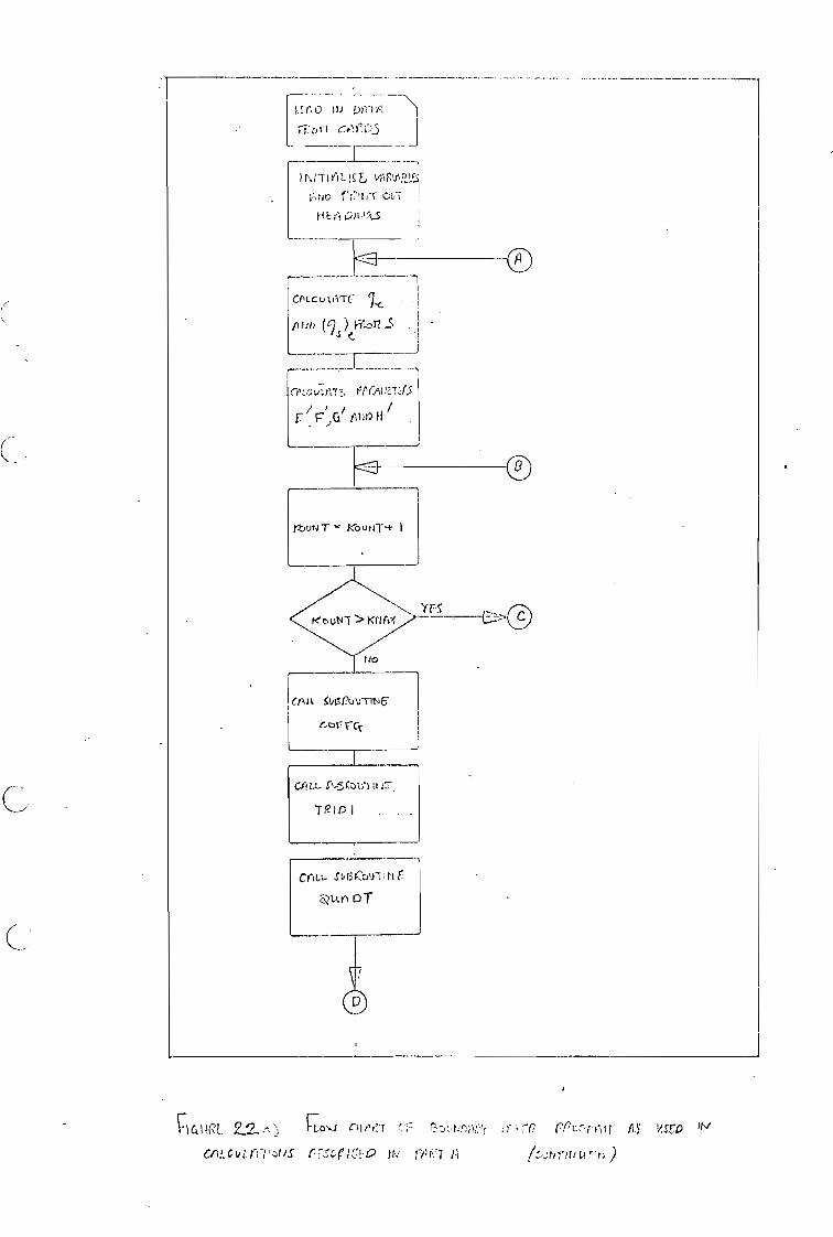
cur c."Ct
criLL sc,( c'fHt tT i
.t.tri DT
CP Lc u LATE 1-c. - - Ma) ) Fito
is n S
1`411' V"i 1_ /SE VASIAP),
No 1";t:1- cl.,-,- ; Fitot:;it ,A.s
r r, 0 III 1,)i-1-1
C1).1')
c:161,(Rt. ("1-) c.r.,ri"01 115 RSCA
cr)Lckitn-p.tiS rrsc-r)c:-o ri, (.1 i )
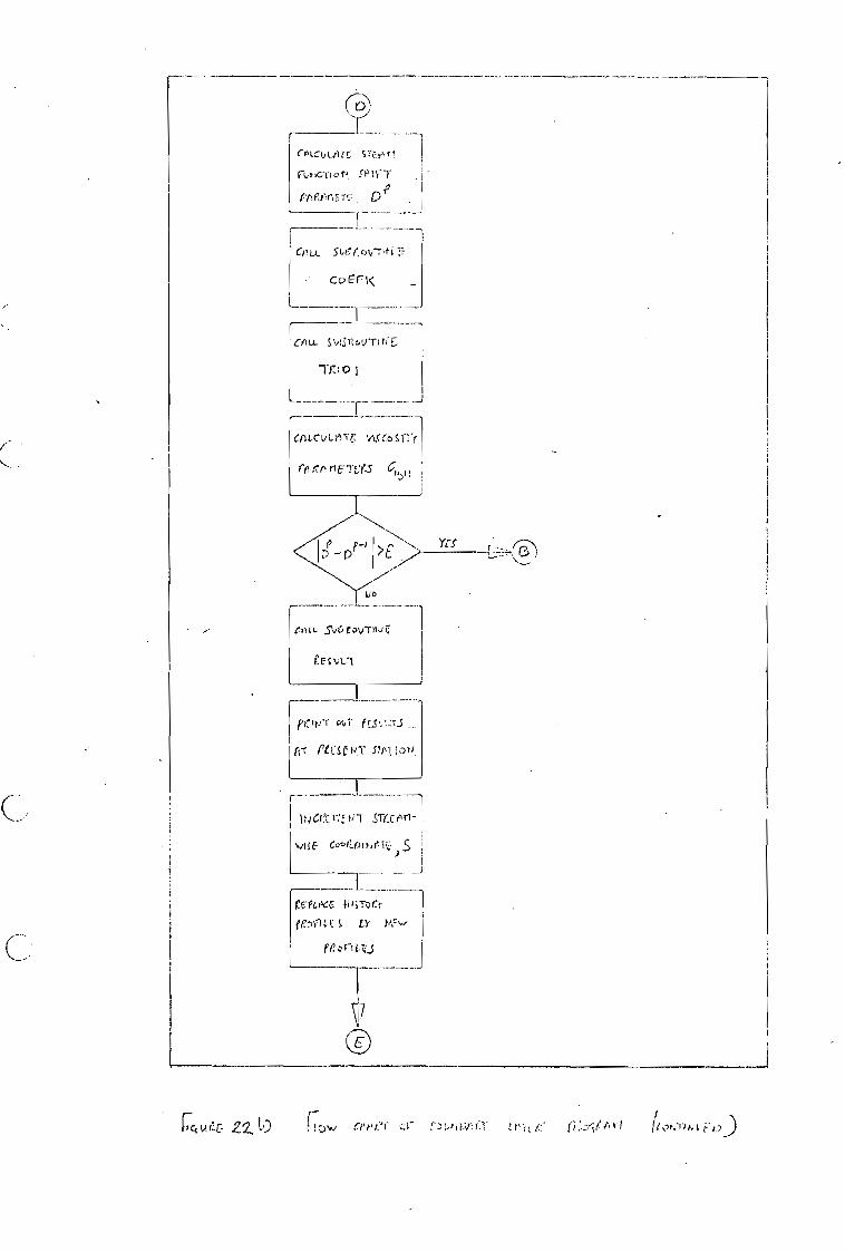
SW:7 IS:AI -TA'
coEnc
T 5
E ET-5
I Yrs DP - P P-I I>E
LID
ett:sc.,141- SinIaN
IN Cet.711E ti 1 ,ST(LC 0 n
\vISE co06.011,,ri - S 1 ) ,
_J 1
rercpcc HIS To rl.- 7
i r? n
vo.c. zz f' ',II 22,r:1-1. r •I W.:4 fog
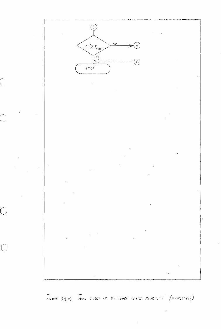
!Yrs
12-4
SI-0P
ric,L1cE
22 c) r-L.‘, r,,._)u,;ppor

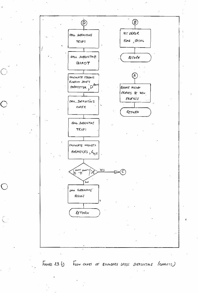
Ye 3
(MICE HIS Tole
Pearl IFS 147v4 frtoricr:s
fErtiglv
et-TokN
mu. SwItto tin 'NE
(?c-.5
staxottriptE
-Ii'! P t
E_
a IAA o
CALGLAAITT ST/Lc-rtri roXil ON Ml 'Fr
g f Ail F-TV1( D
rAtc,vLyr-K. vicc.sri1- reeranzq,ls
IL—ScS ft tTfltf
c?":"F. K
CIAO, 5061.1. 1,11)4 ,17
gqi ,teL t3
raw CA el OF 1:011,1' 1.11Y -Cl; PCADUT ti6 kw1nel FJ
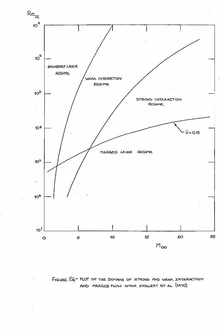
5 0 10 15 2,0
10
106,
BOUNDARY LAYER
REGIME.
STRONG INTERACTION REA1 ME..
10+ ---- 0.15
MERGED LAYER REGIME.
M00
WEAK 1NMRACT/ON REGI ME
105
Rex
riGuRE 24,- PLOT OF THE- DOMAINS OF 5TR3tstCw AND Vig...Ate... INZERACTION
AND MERG-ED FLOW. AFTER STOLLER:I CT AL (1q70)
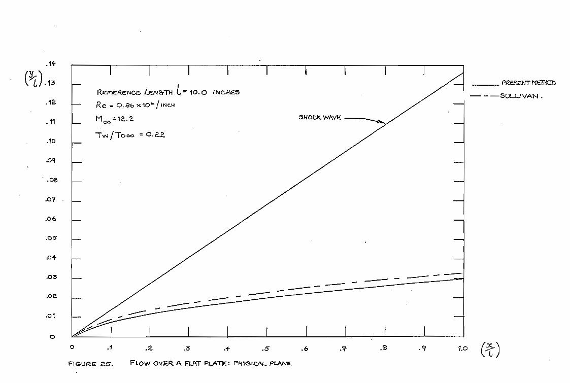
0 .1 .2. .3 .÷ .5 .6 .s .9 1.o
FLOW OVER A FLAT PLATE: PHYSICAL PLANE FIGURE 25.
.12
.11
.10
.09
.08
.07
.06
.05
04
.03
A2
.01
0
PRESENT NETRCID
— —SULLIVAN .
I I I I I I I I
REFERENCE. I.E.nl-TH L17 10-0 INCHES
Re = 0.86 x10b /iNcH
M„=-12..2.
Tw tr000 0.2.2
SHOCK WAVE
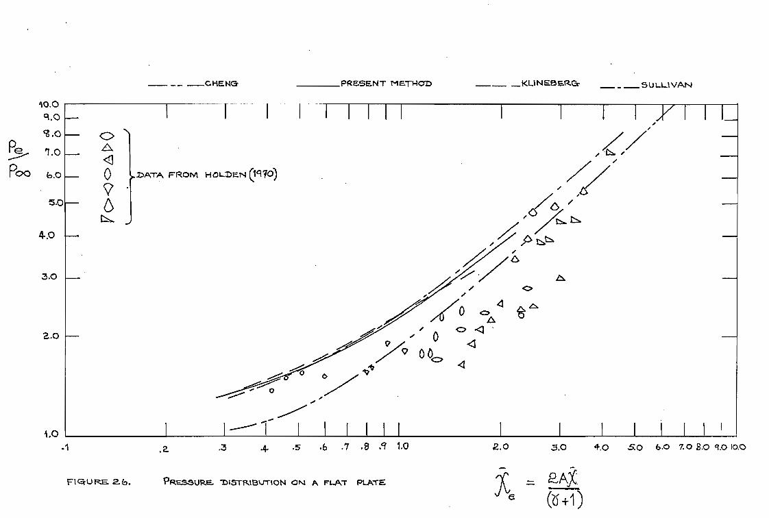
C:>
0
6 L.
9.0 .o
Pe P00 b0
5.0
.DAT'A FROM HOLDEN (1170)
I 1 1 1 1 1 1 1
4.0 —
3.0
2.0
1.0
PRESENT METHOD —KLINEeSS.P.C2- 5 U LLI VAN
.1 .2. .3 .4. .5 .6 .7 .8 1.0 2.0 3.0 4.0 50 6.0 7.0 2.0 9.0 10.0
FR URE.2.6. 'PRESSURE. MISTRIBUTiON ON A FLAT PLATE 2,AX
(6 +1)
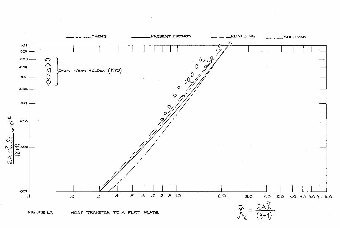
KLI N ESE RG CHENQ PRESENT METH car, SULLIVAN
.01 .00c1
.008
.004
.006
O
4 DATA FROM H OLDEN (1970)
0
.005
.001-
.001 .3 .4 .5 .6 .7 .8 .9 1.0 2.0 3.0 6.0 70 8.0 9.0 10.0
FIGURE TRANSFE...R. ro A FLAT PLATE.
I I 4.0 5.0
.ADC
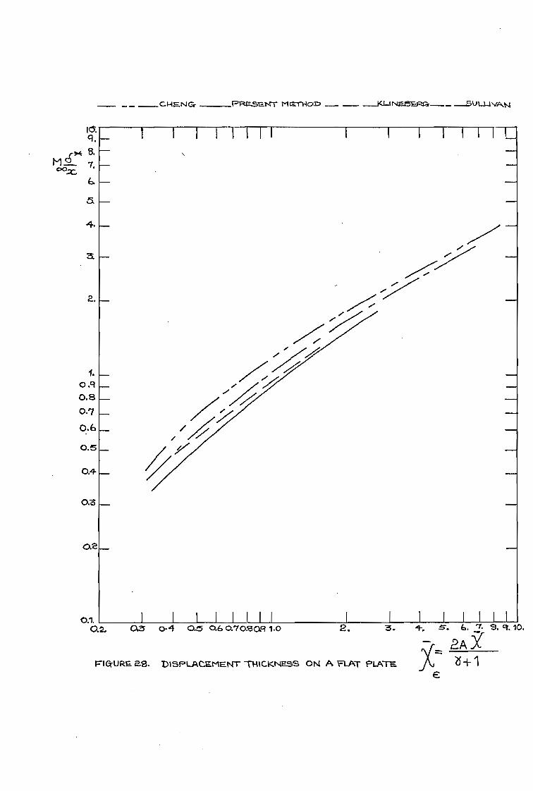
2.
1. o.9 0.8 O.'7
0.6 0.5
0.4
0.3
0.1. 02 0.3 0-4 0.5 0.6 0.70530.4 1.0
— C.1-1 .I■1 Cr PRESS. T41" r**MTHO.T:, — —Kl...( NI.E.....FtGr— - --5U L_L-I VAN
3. 2. 1-.
PICTURE as. DISPLACEMENT 'THICKNESS ON A FLAT PLATE
5-. 6. •1. a 4. 10.
2A Y +1
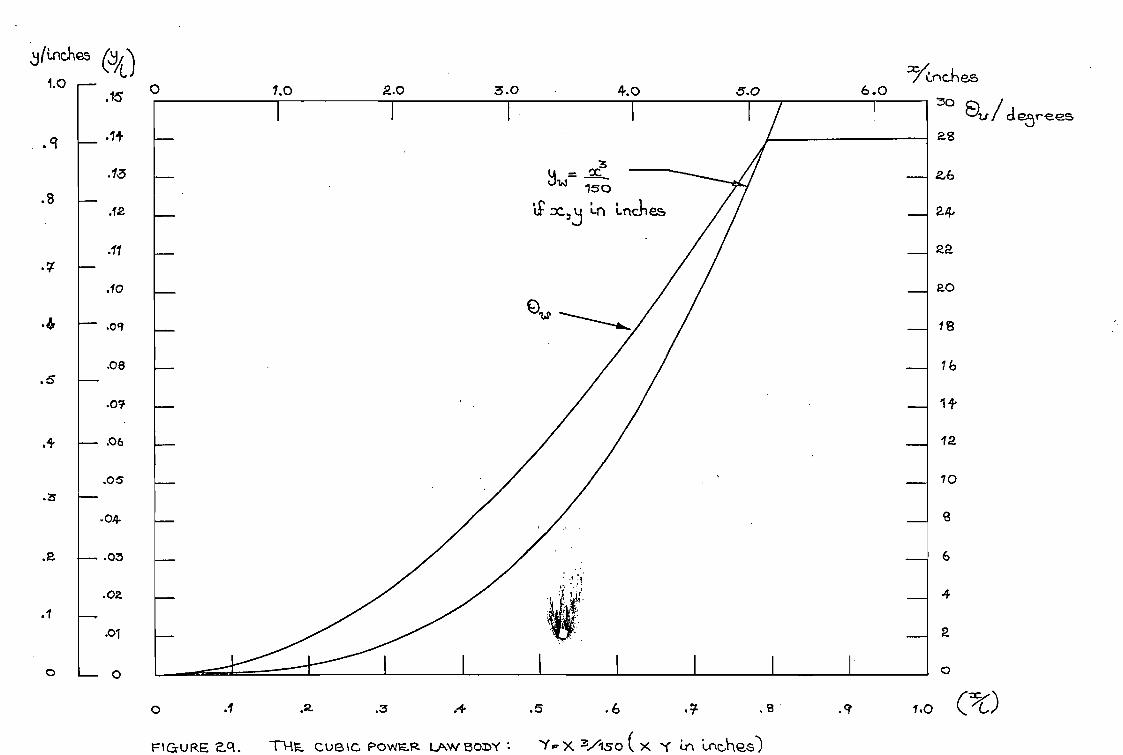
0 V *a' S' a • -4* 9' CI)
Cs'at.pu- Lx? ossVE X Acrocamcn 7:1- mod 'Dien •b-a ain-LDLA
to.
90
90•
b0• 41'
A •
8'
+1.' b
.• 0%9 o• 2 o•v 0'1 p 910 '
C/R) setiouliP
saa-ACcap/rtn ac Lpu')/(x.
0
?1,
9
'tz
8
az
O.9
1. • zo•
co. *a •
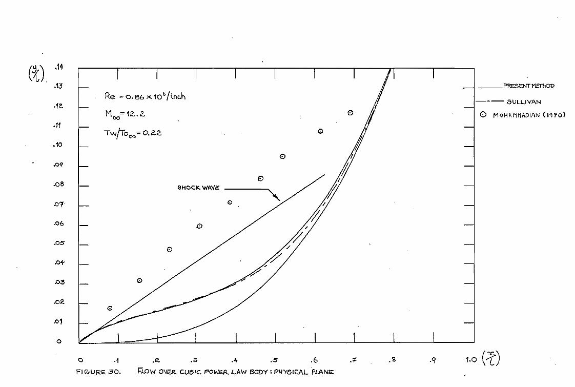
.9 .8 .6 .>~. .3 .4
.11
.10
.08
.07
.06
.05
.03
.02.
.01
0
PR:0■Trti£114^J1)
— 5 U LU VAN
M0101111ADIAN (19?0)
0 .1 FIGURE 30. Row OW..-R. CL/151C PoWW,..R LAW Sony : PHYSICAL PLANE
Re = 0.86 x 1 061inch 1100=12...2.
TwiTocg= 0.22.
O SHOCK WAVE
0
0
0
0
0
0
0
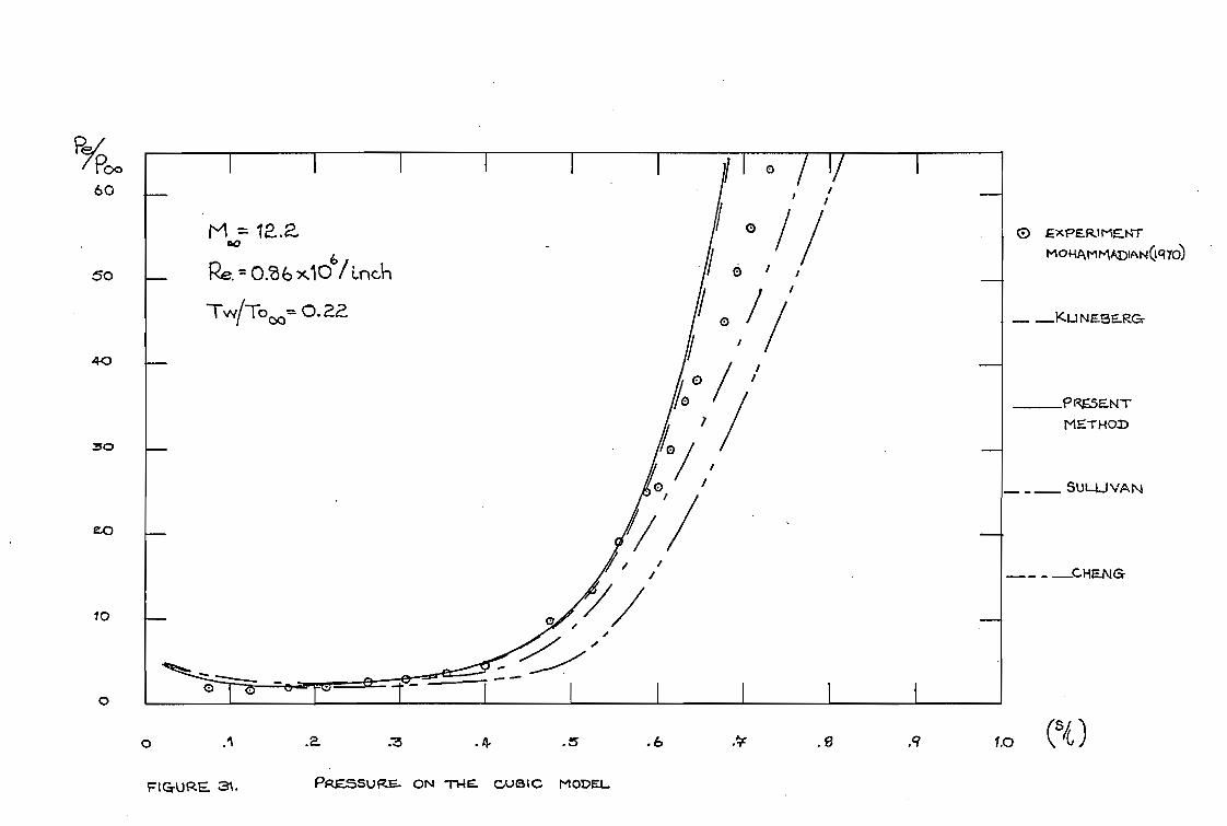
.2. • 4. :3 0 .5 .6 . s .ct
PRE.5SURE. oN -n-15. CUB t C MODEL FIGURE 31.
Proc) 60
50
40
30
10
0
C) xPERINIgt.11- M014/\11 Mialy N(Ici70)
_Ku Na5E.R.Gr
PRE5E.NT MCTHOD
SULLIVAN
— _ CHENG
M = / 0 / 00
Re. = 0.Z 6 x10⁶/ i..ncin 0 /
Tw/Toado= 0.22. I 0 1/
/
//
I I I 1 1
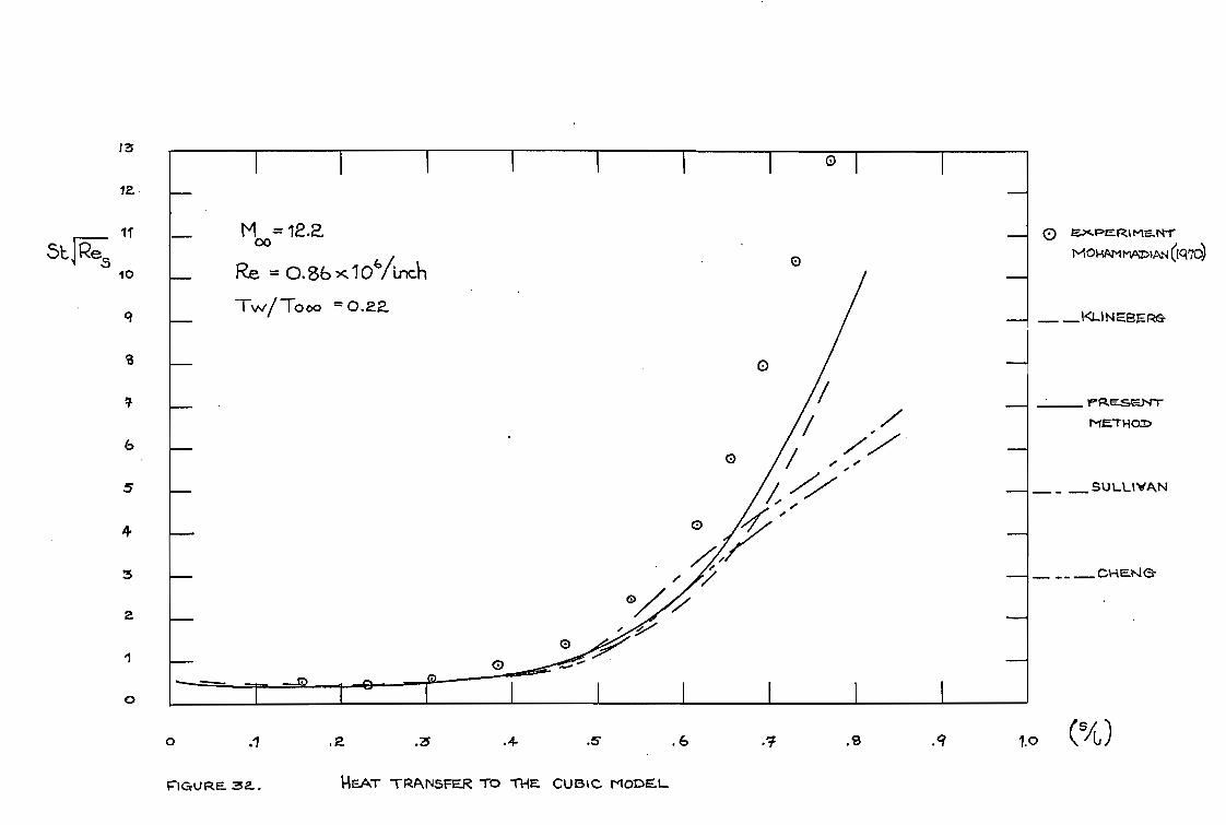
O
Moo= 12.2.
Re = 0.86 x 1 O‘/inch
Tw/ To 00 = 0.22.
CD
0
6
5
4
3
I
0
13
la
Eac.P•MR.1 marsI-r 1•1014X^ImAT);AN (MO)
-K-INE9F.
rcke-smisrr ti="THom
SULLIVAN
o .1 .2. .3 .4 .5 .6 .7 .9 .q 1.0 (54)
F-IURE. 32. NEAT TRANSFER TO THE cur3tc MODEL.
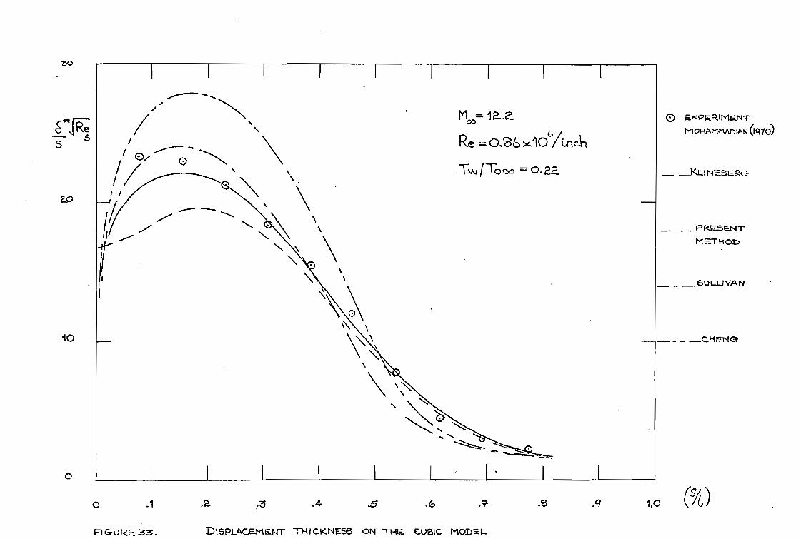
PRFS IT E'T H OD
_ Su U...1 YAN
CHEN G-
1
,<PE.R.IME.NT Mot4AmmazNANI Oct 7'0)
_KLINESERC- I 0/ 0-
7
Moo= 1a..a
Re = 0.88 >4.10‘ And-1
Tw To = 0. 22.
0 .1 .2 .3 .4 .5 4 .7 .8 1,0 (SA)
FIGURE 33. DISPLACEMENT TH I CKNE% ON THC CUt3IC MODEL_
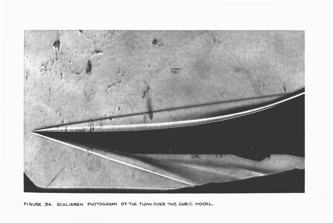
• •-i-aciot4 o 1 iimo -la hi_ -0s3AO N\CTIA "aii.1.. A.0 Hakrel-nO.L011c1 N'atf5 I -1H'JS
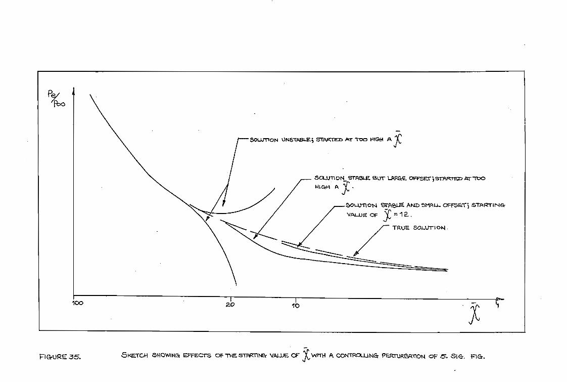
FIGURE 35. 51.e.s-rcm SHOWING EFFEL-I s OF THE STARTING VALUE. CF'
ITH A OZWIROLLING PERTUReATION OF 6. SIG. FIG.
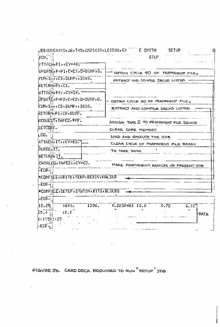
IJ0ECUMEA005, J6, T45, CM2S000, LC1500/ G> E SMITH SETUP
EOX;i=1
STOP
ATTPCH !PI, 5CY=40. ,
0PDA119, P=P1 9 C=-C 1 50=DUMPs Q.
5' C / v DUMP, 9 3 0 0 0 . I ....L___
-ETOkisi,P19c1. _VI
A
PttriCti, P2 9 CY=3 CI.
bPDA:t!6F=P2,C=C2, 0=PUMPIO. 1 -f1
C2v DUMP/1'3000. ,I::;' rA
EXTRACT AND COMPILm. •DEC.}‹.5 L4STEI>.
'RETURN', P2 5 Ca J DUMP.
lig - ft•A
:EQUEST P TAPE2 k:-PF-. ASSIGN TAPE 2. TO PERMANENT FILE 1::\IICE- 1 •
CLEAR CORE. MET-10R.Y.
Lo AD AND exscuTE -rvm. z-oe,
CLEAR CNCL.E. OF PC..-RMANENT PL REAVY
TO TAKE.. DATA
MAKE PERMANC-.NTRF-.50L..7-5 OF PRESENT aoEs
t.Oil- ILEP WRITES TERP,VER I V A HALSUE
EOR-I_ i
COMPIiLE, SETUPS STWTSN B ffS s ELSUITS
-ECIR:1„1
L 1600. 1300. 0.2238461 10.0 ..
. ID :
0( Cr. 5C,C I 25
-
SETCOR.E. • • ....-1:2_L:.-.L._ 60. • ,
AtTACH, IT, II CY=6,:,.- . I..1 .. ..
'UR-C;BriIT.
IRETURINt ,IT.
liCi=ITLLOIG, TAPE2r / CY=63.
-
C. 2
013-rizoN CYCLE. 40 OF PERMANENT FILE*
EXTRACT" AND CCMP1LE. -DEC.AcS U5TE3D
— OBTAIN CYCLE 5O OF PERMANENT FILE.,
FI G-U RE 3b. CARD DECK REQU RED TO RUN TUP SOB
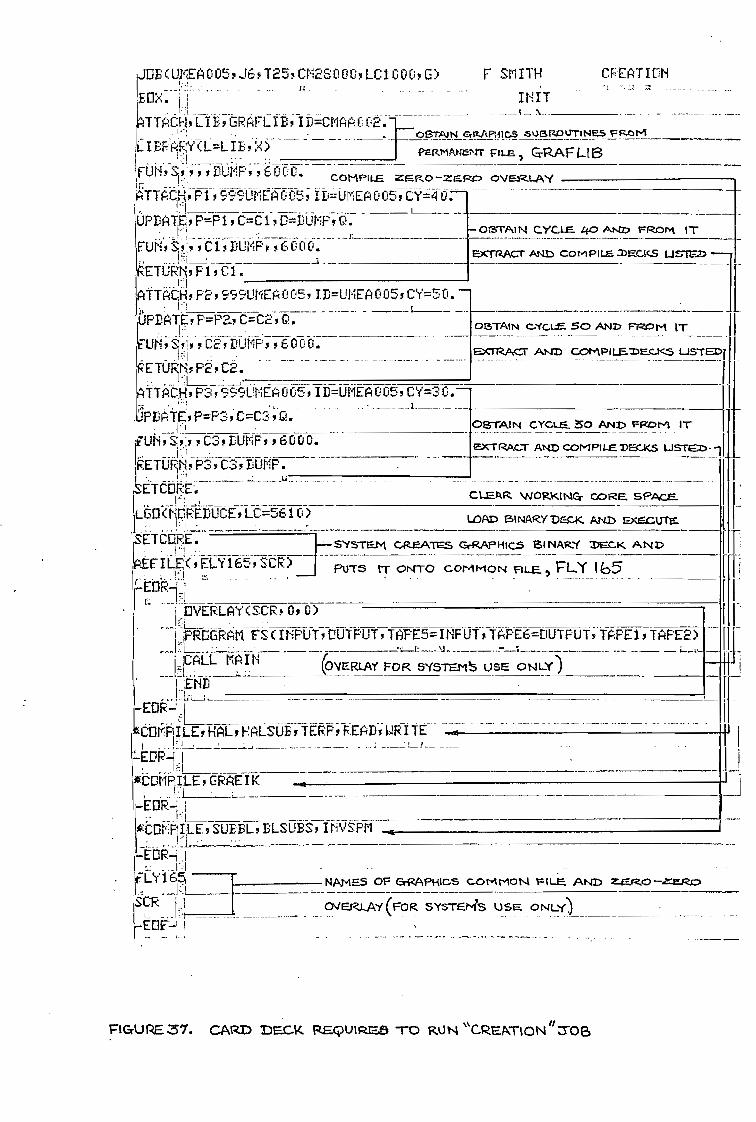
EXTRACT AND COMPILE MECKS USir..D i
1
IJOB<U1NEA 005$ J6 t T.2.5 t CM28000t LC1000$ G) F SMITH IE.OX. 1. 1 INIT ATTACH', L I B9 GRAFLI B1 I D=CM . AA002 ____
. I- OBTAIN CrItAPHIc...S k.+E.F...0%-rri Nes FP..ordi ICIEPARY(L=LIE)- Partmmatsrr nix: I GRAF I-10 1 • - - 'Flii-4 SO y ; DUMP 7 E. OtZ COMPILE E.P..0-ZE.R.c, OVERLAY H! 4TTACH$ P 1 , 99UMEA 005 $ I Ii7UMEA 005 v C1..Y=_ 40.
'UPDATE. P=P 1, C=C130=DUMPI Q. I. 11 FUMPS
'
Y liCI:SDUMF.-'$ f6000a
g l:1 :ETURN,, F 1 9C1 .
, ___L! _ , JATTACH$ P2, 999LIMEA 005 $ I D=UMEA005 s CY=.5 O. —
1--, L______ -1..IPDAT, P=P3.$ C=C2 $ C.
1":1 -LIN/ SI1 5 C21 DUMP y t 6000.
IR41ETU: P2, C2. ATTACH: P3 , ".995,,LIMEA 005 " I D=UMEA 0059CY=30. ,•-■ UPDATE; P-=P3, C=C3; Q.
• • 1 - I UN; 5;::y 1 C3: LUMP: 16000.
C3
kTCOE'. 6OfillUCE,LC=5610)
ETCORE. • i 1 • • FILE ,ELY16 , SCR )
kEvIERLAY (SCR IL 090) kriRpGRAM FS( INPUT, OUTPUT, TAFE5= I NF UT ; TAPE6=OUTPUT, TAPE1 F TAPE2)
- I, \I - 1 i--,-LL kiCALL—fileA I N (OVERLAY FOR SYSTEM USE ONLY) I bit
■Ok
NNAES OF G-RAPHICS COMMON FILE AND Z.E.920 -•r-ERO
OVERLAY (FOR SYSTEM'S USE ONLY')
CREATION
OLSTAIN CYCLE 40 AND FROM IT
EXTRACT AND COMPILEMECKS USTE2Or
OBTAIN CAfc,t_.E. 50 AND FTs'M IT
rt
EOR-11 , _ 1-rt____
.CCIMPIi LE, HAL il, FALSUE, TERP y READ: WRITE -4
1 L ,..,l' . - • i H !.. ILEE1R-41 L--;.1 rC0i±P1-' ILE I GRAFI K
_, ......_ =-E.ER.--i
- _ 1 -- tni<P,I;LE, SUEEL P DLSUES , I NVSPM
-_ , , - ______________ •
SYSTEM CREATES GrRAPHIC5 BI NARY iC.K AND
Pu-rs t7 ONTO COMMON FILE. FLY 165
LOAD BINARY DECK AND EXECUTE.
CLEAR \NORKIN*- CORE SPAcE.
OBTAIN CYCLE 50 AND FROM IT EXTRACT AND COMPILE DECKS LJSTEA.
1i
FIG-URE.Z7. CARD DECK REQUitZENS TO RUN %%CREATION" 3-0 B
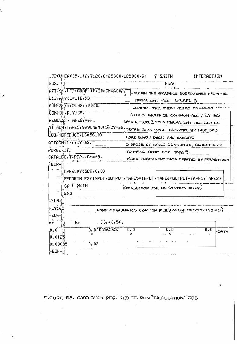
GRAF
-OBTAIN 11-4E G-RAPHICS SUCSROu-rINIES FROM 'T-HE
PERMANENT FILE CTRAFLIB
DE(UMEA005$J121T120$CME5GCOILC5000$G) F SMITH INTERACTION lEnk.
')TTAC+-1$ L IT5$ GRAELIE$ IL=CMAA 0 02.—
IBRARY(L=LIE$ X)
EU, ,I5UMP, EOCJJ. 1=1 comPit..E. THE. Z.E.R0 -Z.ERo OVERLAY COMMON FLY165.. ATTACI-I GRAPHICS COMMON FILE ,FLY 15 REQUES,T$ TAPE2 9 #PF. A55IGrN TAM 2, To A M.RmANE.r•Ii" FILE IDEV C.E T"TACH; TAPE1-$ 999UMEA 0 C.5; CY=62* OBTAIN DATA 13 AsE. c.REATED lEI`( LAST 50e> C-0$ NOREDUCE$ LC:=5610) LOAD BINARY .C-K AND E.K.r_c.trre
AtTi=itkif If/ ;rt.11=63. ISPOS E OF CYCLE CONITAIN tr.* OLDEST DATA
TO MAKE ROOM FOR TAPE e• CAT1# PTAPE2 $ CY=63. palarickwarrr 1!)ATA CREATED BY PReSENTUOB EOR*I
.OVERLAY(SCRI 0, 0)
f ROGRATI FS( INPUT, DUTPUTP TAPE5= I NPUT TAPE6=DUTPUTP TAPE I TAPE2) :-. • .. . . .1 E
JCALL MAIN
END
EOR-21 ritkele p H . . -E0R-i i
71 63
O. H
0..000,05
(OVERLAy FOR USE OF SVSTEM ONL.X)
NAmE. OF GRAPHICS CoMmoN FILE_ (FORUSE. OF SYSTEM ONLY)
0.0000365E57 0.0 0.0
0. 0 DATA
0.02
flGuR.38. CARD DECK REQUIRED TO FZUN "CALCULATION" 3.08