The Nucleus of Interstellar Comet 2I/Borisov

David Jewitt1,2, Man-To Hui3, Yoonyoung Kim4, Max Mutchler5, Harold Weaver6 and

Jessica Agarwal4

1 Department of Earth, Planetary and Space Sciences, UCLA, Los Angeles, CA 90095-1567

2 Department of Physics and Astronomy, UCLA, Los Angeles, CA 90095-1547

3Institute for Astronomy, University of Hawaii, Honolulu, Hawaii 96822

4 Max Planck Institute for Solar System Research, 37077 Gottingen, Germany

5 Space Telescope Science Institute, Baltimore, MD 21218

6 The Johns Hopkins University Applied Physics Laboratory, Laurel, Maryland 20723

jewitt@ucla.edu

Received ; accepted

Astrophysical Journal Letters, in press

arX

iv:1

912.

0542

2v2

[as

tro-

ph.E

P] 8

Jan

202

0

– 2 –

ABSTRACT

We present high resolution imaging observations of interstellar comet

2I/Borisov (formerly C/2019 Q4) obtained using the Hubble Space Telescope.

Scattering from the comet is dominated by a coma of large particles (character-

istic size ∼0.1 mm) ejected anisotropically. Convolution modeling of the coma

surface brightness profile sets a robust limit to the spherical-equivalent nucleus

radius rn ≤ 0.5 km (geometric albedo 0.04 assumed). We obtain an independent

constraint based on the non-gravitational acceleration of the nucleus, finding

rn > 0.2 km (nucleus density ρ = 500 kg m−3 assumed). The profile and the

non-gravitational constraints cannot be simultaneously satisfied if ρ ≤ 25 kg m−3;

the nucleus of comet Borisov cannot be a low density fractal assemblage of the

type proposed elsewhere for the nucleus of 1I/’Oumuamua. We show that the

spin-up timescale to outgassing torques, even at the measured low production

rates, is comparable to or shorter than the residence time in the Sun’s water sub-

limation zone. The spin angular momentum of the nucleus should be changed

significantly during the current solar fly-by. Lastly, we find that the differential

interstellar size distribution in the 0.5 mm to 100 m size range can be represented

by power laws with indices < 4 and that interstellar bodies of 100 m size scale

strike Earth every one to two hundred million years.

Subject headings: comets: general — comets: 2I/2019 Q4 Borisov

– 3 –

1. INTRODUCTION

Comet 2I/Borisov (hereafter simply “2I”) is the second interstellar interloper detected

in the solar system, after 1I/’Oumuamua (“1I”). Scientific interest in these bodies lies in

their role as the first known members of an entirely new population formed, presumably,

by the ejection of planetesimals in the clearing phase of external protoplanetary disks

(e.g. Moro-Martin 2018). Curiously, the first two interstellar objects appear physically quite

different. Whereas ’Oumuamua was an apparently inactive, roughly 100 m scale body with

a large amplitude lightcurve (Bannister et al. 2017, Jewitt et al. 2017, Meech et al. 2017,

Drahus et al. 2018) 2I more closely resembles a typical solar system comet, with a prominent

dust coma that was evident at discovery (Bolin et al. 2019, Guzik et al. 2019, Jewitt and

Luu 2019) and weak spectral lines (Fitzsimmons et al. 2019, McKay et al. 2019) indicative

of on-going activity. Despite appearing inactive, comet 1I exhibited non-gravitational

acceleration (Micheli et al. 2018), likely caused by recoil forces from anisotropic mass loss

(although other explanations have been advanced; Bialy and Loeb 2018, Moro-Martin 2019,

Flekkoy et al. 2019).

Comet 2I passed perihelion on UT 2019 December 8 at distance q = 2.006 AU and

will reach Jupiter’s distance in 2020 July and Saturn’s by 2021 March. Here, we present

pre-perihelion Hubble Space Telescope (HST) observations at heliocentric distance rH =

2.369 AU. A particular objective is to determine the effective size of the nucleus using the

highest resolution data.

2. OBSERVATIONS

All observations were obtained under the Director’s Discretionary Time allocation

GO 16009. We used the WFC3 charge-coupled device (CCD) camera on HST, which has

– 4 –

pixels 0.04′′ wide and gives a Nyquist-sampled resolution of about 0.08′′ (corresponding

to 160 km at the distance of 2I). In order to fit more exposures into the allocated time,

only half of one of two WFC3 CCDs was read-out, providing an 80” x 80” field of view,

with 2I approximately centrally located. The telescope was tracked at the instantaneous

non-sidereal rate of the comet (up to about 100′′ hour−1) and also dithered to mitigate

the effects of bad pixels. All data were taken through the F350LP filter, which has peak

transmission ∼ 28%, an effective wavelength λe ∼ 5846A, and a full width at half maximum,

FHWM ∼ 4758A. In each of four orbits, we obtained six images each of 260 s duration.

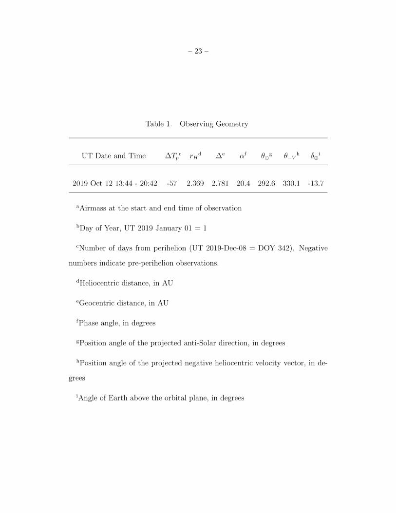
Geometric parameters of the observations are summarized in Table (1).

3. DISCUSSION

Morphology:

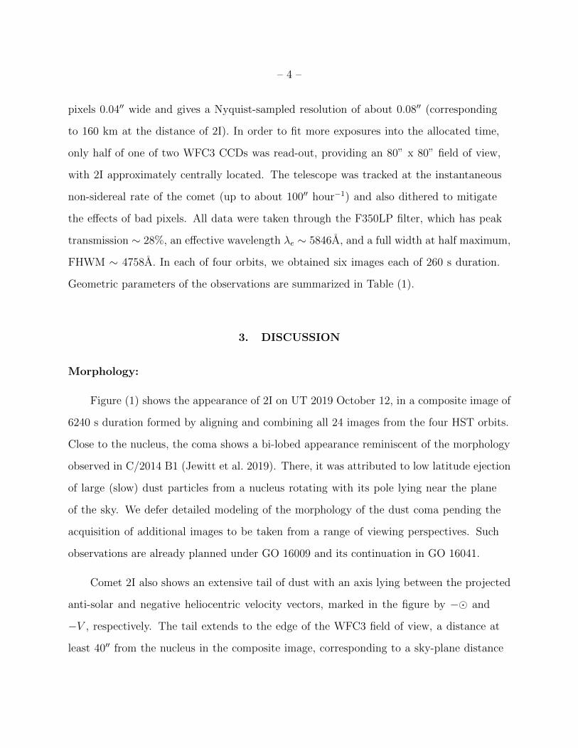
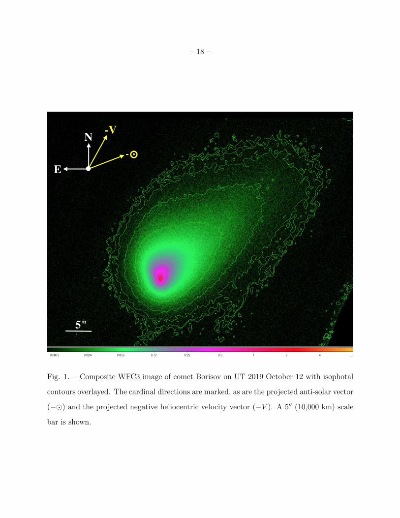
Figure (1) shows the appearance of 2I on UT 2019 October 12, in a composite image of

6240 s duration formed by aligning and combining all 24 images from the four HST orbits.

Close to the nucleus, the coma shows a bi-lobed appearance reminiscent of the morphology

observed in C/2014 B1 (Jewitt et al. 2019). There, it was attributed to low latitude ejection

of large (slow) dust particles from a nucleus rotating with its pole lying near the plane

of the sky. We defer detailed modeling of the morphology of the dust coma pending the

acquisition of additional images to be taken from a range of viewing perspectives. Such

observations are already planned under GO 16009 and its continuation in GO 16041.

Comet 2I also shows an extensive tail of dust with an axis lying between the projected

anti-solar and negative heliocentric velocity vectors, marked in the figure by −� and

−V , respectively. The tail extends to the edge of the WFC3 field of view, a distance at

least 40′′ from the nucleus in the composite image, corresponding to a sky-plane distance

– 5 –

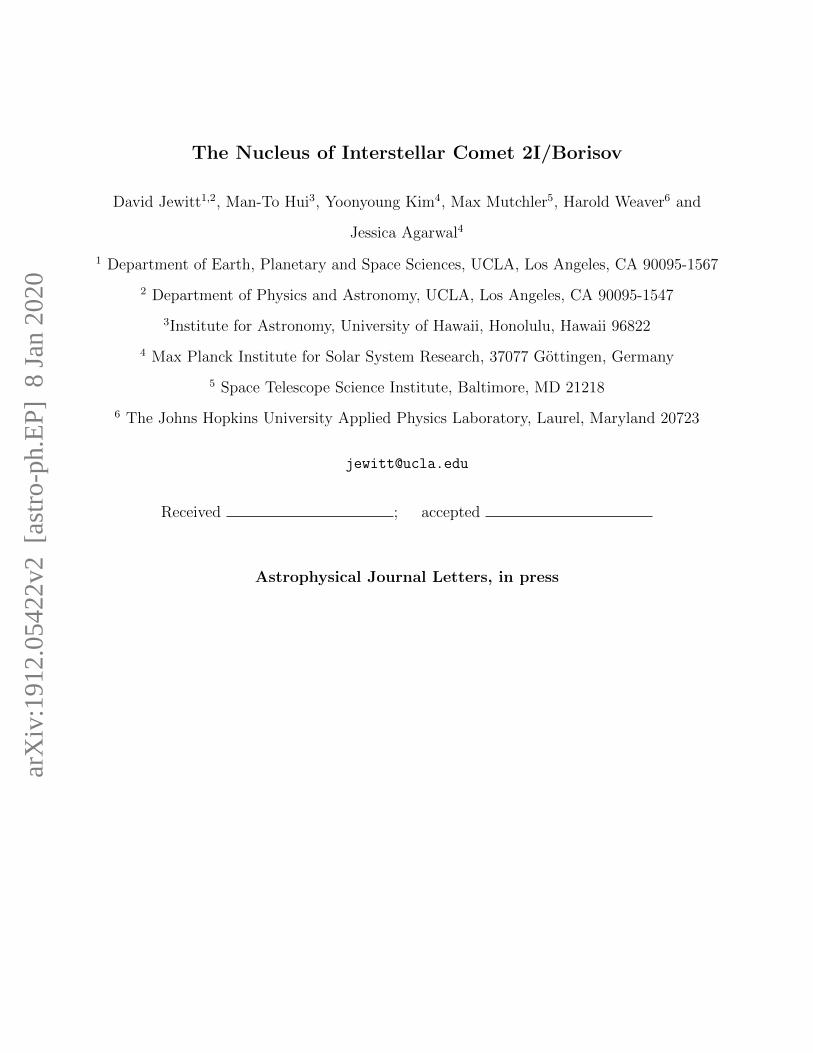
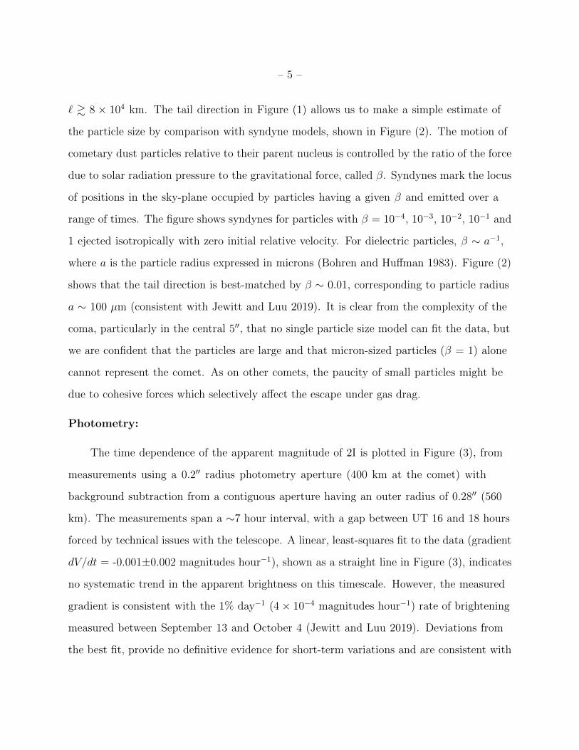
` & 8 × 104 km. The tail direction in Figure (1) allows us to make a simple estimate of

the particle size by comparison with syndyne models, shown in Figure (2). The motion of

cometary dust particles relative to their parent nucleus is controlled by the ratio of the force

due to solar radiation pressure to the gravitational force, called β. Syndynes mark the locus

of positions in the sky-plane occupied by particles having a given β and emitted over a

range of times. The figure shows syndynes for particles with β = 10−4, 10−3, 10−2, 10−1 and

1 ejected isotropically with zero initial relative velocity. For dielectric particles, β ∼ a−1,

where a is the particle radius expressed in microns (Bohren and Huffman 1983). Figure (2)

shows that the tail direction is best-matched by β ∼ 0.01, corresponding to particle radius

a ∼ 100 µm (consistent with Jewitt and Luu 2019). It is clear from the complexity of the

coma, particularly in the central 5′′, that no single particle size model can fit the data, but

we are confident that the particles are large and that micron-sized particles (β = 1) alone

cannot represent the comet. As on other comets, the paucity of small particles might be

due to cohesive forces which selectively affect the escape under gas drag.

Photometry:

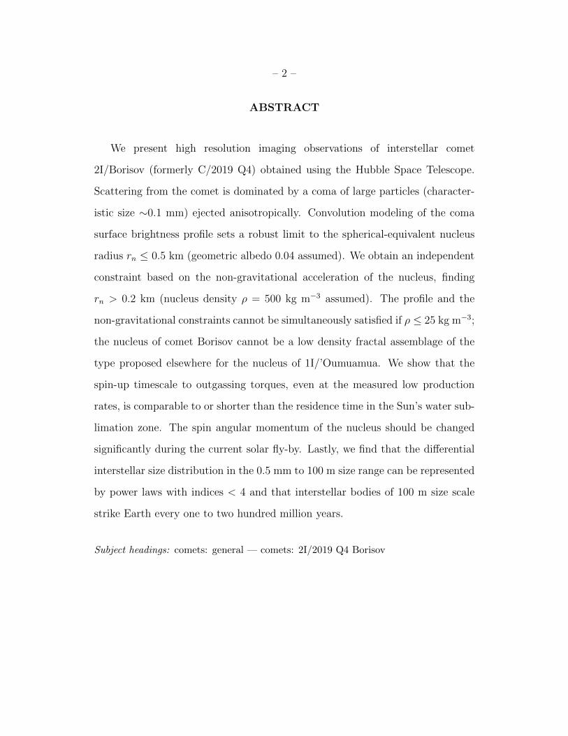
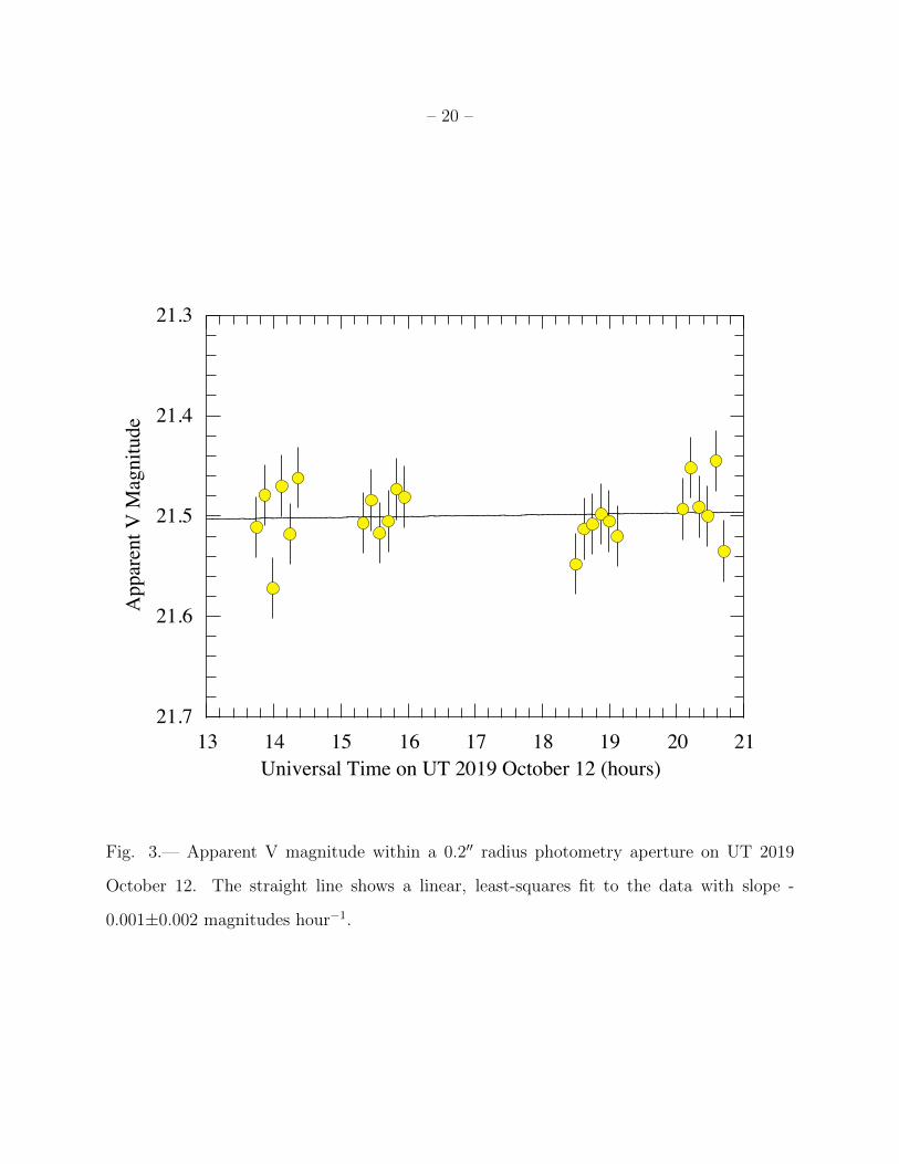
The time dependence of the apparent magnitude of 2I is plotted in Figure (3), from

measurements using a 0.2′′ radius photometry aperture (400 km at the comet) with

background subtraction from a contiguous aperture having an outer radius of 0.28′′ (560

km). The measurements span a ∼7 hour interval, with a gap between UT 16 and 18 hours

forced by technical issues with the telescope. A linear, least-squares fit to the data (gradient

dV/dt = -0.001±0.002 magnitudes hour−1), shown as a straight line in Figure (3), indicates

no systematic trend in the apparent brightness on this timescale. However, the measured

gradient is consistent with the 1% day−1 (4× 10−4 magnitudes hour−1) rate of brightening

measured between September 13 and October 4 (Jewitt and Luu 2019). Deviations from

the best fit, provide no definitive evidence for short-term variations and are consistent with

– 6 –

the 1σ = ±0.03 magnitude statistical errors. We thus find no evidence for modulation

of the light scattered from an ’Oumuamua-like rotating, aspherical nucleus. As we show

below, the most likely explanation is coma dilution within the 0.2′′ photometry aperture,

because the cross-section of the nucleus is small compared to the combined cross-sections of

the dust particles within the projected aperture.

Crude Radius Estimate: The best-fit value of the apparent magnitude from Figure (3)

is V = 21.51±0.04. The absolute magnitude computed from V assuming a linear phase

function of the form Φ(α) = 0.04 magnitudes degree−1 is H = 16.60 ± 0.04 magnitudes,

where the quoted uncertainty reflects only statistical fluctuations. Uncertainties in the

phase function are systematic in nature and dominate the statistical errors. For example,

plausible uncertainties in Φ(α) of ±0.02 magnitudes degree−1 affect our best estimate of H

by ±0.4 magnitudes.

The scattering cross-section corresponding to H, in km2, is calculated from

Ce =1.5× 106

pV10−0.4H (1)

where pV is the geometric albedo. The mean albedo of cometary nuclei is pV ∼ 0.04

(Fernandez et al. 2013) and, using this albedo, Equation (1) gives Ce = 8.6 km2. The

radius of an equal-area circle is re = (Ce/π)1/2, or re = 1.6 km. This constitutes a crude

but absolute upper limit to the radius of the nucleus, because the central 0.2′′ aperture is

strongly contaminated by dust.

Radius from Profile Fitting: To better remove the dust contamination of the

near-nucleus region, we fitted a surface brightness model to the coma and extrapolated

inwards to the location of the nucleus, according to the prescription described in Hui and

Li (2018). For this purpose, the surface brightness was fitted in 1◦ azimuthal segments

– 7 –

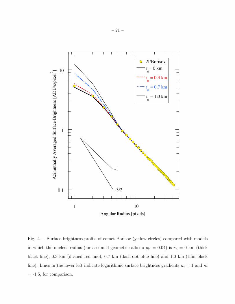
over the radius range 0.24′′ to 1.20′′. The weighted mean surface brightness within a set of

nested annuli is shown in Figure (4). Statistical error bars, computed from the standard

error on the mean of the value at each radius, are smaller than the plot symbols. Systematic

errors, principally due to uncertainties in the background subtraction due to field objects

and internal scattering, were found to be unimportant in the fitted region of the profile.

Consistent profiles were obtained using data from the other three HST orbits and so these

are not shown separately.

The fitted profiles were then convolved with the HST point spread function provided

by TinyTim (Krist et al. 2011), after adding a central point source signal to represent the

nucleus. In the figure we show models in which the effective nucleus radii are rn = 0, 0.3,

0.7 and 1.0 km, respectively (albedo pV = 0.04 assumed). By inspection of the figure, we

conservatively set an empirical upper limit to the radius of the nucleus rn ≤ 0.5 km, far

smaller than the crude estimate given above and showing the importance of accurate dust

subtraction.

Other Radius Constraints: Two other observations can be used to independently

constrain the radius of the nucleus of 2I, although neither is as robust as the limit derived

from the surface brightness profile. Both are based on knowledge of the mass production

rate of 2I.

Cometary non-gravitational motion provides a measure of the nucleus size, essentially

because the sublimation rate is proportional to r2n while the mass is proportional to r3n.

Small nuclei can be measurably accelerated by recoil forces from anisotropic sublimation

while large nuclei cannot. The recoil force resulting from the loss of mass at rate M and at

speed Vth is F = fngMVth, where 0 ≤ fng ≤ 1 is a dimensionless number representing the

degree of anisotropy of the mass loss. Isotropic emission, corresponding to zero net force on

the nucleus, has fng = 0, while perfectly collimated emission has fng = 1. Observations show

– 8 –

that sublimation-driven mass loss from comets is highly anisotropic, occurring primarily

from the sun-facing hemisphere. Through Newton’s law, we set F = 4π/3 ρr3nA, where A is

the non-gravitational acceleration [m s−2] of the nucleus. The effective radius of the nucleus

is then given by

rn =

(3fngMVth

4πρA

)1/3

(2)

We use the mean thermal speed of molecules Vth = (8kT/(πµmH))1/2, where µ = 18 is

the molecular weight of H2O, mH = 1.67× 10−27 kg is the mass of the hydrogen atom and

T is the temperature of the sublimating surface, which we calculated from the equilibrium

sublimation condition (T = 197 K at 2 AU). We find Vth = 480 m s−1. The nucleus density

was assumed to be ρ = 500 kg m−3 (Groussin et al. 2019).

The most direct estimates of the 2I mass loss rate, M , are provided by spectroscopic

detections of the forbidden oxygen ([OI]6300A) line, which give QH2O = (6.3± 1.5)× 1026

(M = 20±5 kg s−1) at rH = 2.38 AU (McKay et al. 2019). Less direct but broadly consistent

estimates are provided by the resonant fluorescence band of CN3880A (Fitzsimmons et

al. 2019). When scaled to OH rates using factors determined in solar system comets (A’Hearn

et al. 1995), the CN detection gives water production rates QH2O = (1.3− 5.1)× 1027 s−1,

corresponding to 40 ≤ M ≤ 150 kg s−1 at rH = 2.66 AU. Of these two measurements, we

consider the one based on [OI] more likely to be accurate, given that the determination

from CN is one additional step removed by the unmeasured OH/CN ratio.

Astrometric data provide a measure of A, with the major limitation that, at the time

of writing, the resulting deviations from purely gravitational orbit solutions are modest

(1′′ to 2′′), and the estimation of A is therefore sensitive to astrometric uncertainties as well

as to the force model employed. The solutions are particularly sensitive to pre-discovery

– 9 –

observations reported by Ye et al. (2019), some of which appear questionable given the low

signal-to-noise ratios in their data.

The most recent available orbit solution is JPL Horizons orbit#48 (dated 2019

December 09), which uses astrometry obtained between UT 2018 December 13 and 2019

December 4. The solution gives A1 = −9.1× 10−8, A2 = 2.3× 10−8 and A3 = −1.2× 10−7.

Using the force model of Marsden et al. (1973), the derived acceleration of the nucleus is

A = 8 × 10−7 m s−2 at rH = 2 AU. To check this, one of us (Man-To Hui) fitted a high

quality sub-set of the astrometric data (enlarged to include astrometry up to 2019 December

8 ) to obtain A1 = (7.1± 7.1)× 10−8, A2 = (1.0± 1.0)× 10−7 and A3 = (−1.6± 1.9)× 10−8,

where the quoted uncertainties are 1σ standard deviations. In view of the errors, the fit

indicates that the three components are not statistically different from zero. Therefore, we

combined the measured values in quadrature to obtain a 3σ limit to the acceleration at

rH = 2.00 AU, A < 7 × 10−7 m s−2. This is numerically close to the value obtained from

JPL#48, but is interpreted as an upper limit to A rather than a detection of it.

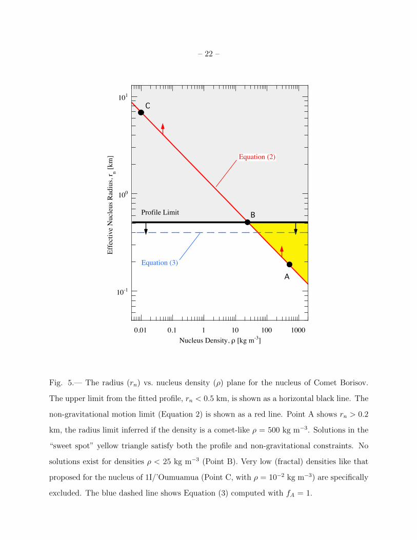
With A < 7× 10−7 m s−2, nominal density ρ = 500 kg m−3 (Groussin et al. 2019), and

fng = 1, Equation (2) gives rn > 0.2 km (point A in Figure 5). This value is consistent with

rn < 0.5 km as obtained from the surface brightness profile and neatly brackets the nucleus

radius, 0.2 ≤ rn ≤ 0.5 km, provided ρ = 500 kg m−3. However, since the density of 2I is

unmeasured, we must also consider other values. In order to satisfy the profile constraint

(rn < 0.5 km) while keeping M and A as measured, Equation (2) requires ρ > 25 kg m−3

(point B in Figure 5). This is interesting because much lower densities (e.g. ρ = 10−2 kg

m−3) have been posited in fractal models of the non-gravitational acceleration of the nucleus

of 1I (Flekkøy et al. 2019, Moro-Martin 2019). Such low densities, when substituted into

(Equation 2) would give rn > 7 km, strongly violating the rn < 0.5 km limit obtained from

the surface brightness profile (point C in Figure 5).

– 10 –

The third and weakest constraint on the nucleus radius is based on the production of

gas. The rate of sublimation in equilibrium with sunlight is proportional to the sublimating

area according to

rn =

(M

2πfAfs

)1/2

. (3)

Here, fA > 0 is the active fraction of the sun-facing hemisphere and fs [kg m−2 s−1] is the

specific rate of sublimation. We solved the equilibrium energy balance equation for water

ice sublimation, neglecting conduction, assuming heating of the sun-facing hemisphere of

the nucleus. At rH = 2.38 AU, the specific rate is fs = 2 × 10−5 kg m−2 s−1, rising to

fs = 3× 10−5 kg m−2 s−1 at perihelion. Substituting active fraction fA = 1, Equation (3)

gives a nominal radius rn = 0.4 km, neatly falling between the bounds set by the profile

and the non-gravitational solutions (for ρ = 500 kg m−3). However, the value of the active

fraction, fA, is not measured in 2I. In well-measured solar system comets, this quantity is

widely scattered from fA . 10−2 to fA ≥ 1, with a tendency to be larger for smaller nuclei

(A’Hearn et al. 1995). Values fA < 1 are possible if the nucleus is largely inert, allowing

solutions with larger rn by Equation (3). Values fA ≥ 1 are possible when the measured gas

is produced in part, or in all, by sublimation from grains in the coma (c.f. Sekanina 2019),

allowing solutions with smaller rn. For these reasons, while noting the amazing concordance

between estimates of the nucleus radius obtained from the three different methods, we

consider the radius constraint from Equation (3) to be the weakest of the three presented

here.

– 11 –

3.1. Spin-Up, Size Distribution and Impact Flux

The upper limit to the radius obtained using HST is an order of magnitude smaller

than limits from ground-based data (e.g. rn . 7 km, Ye et al. 2019). This small radius

renders the nucleus of 2I susceptible to rapid changes in the spin state as a result of

outgassing torques (Jewitt and Luu 2019). The e-folding spin-up timescale for these torques

is

τs =ωρr4n

kTVthM(4)

in which ω = 2π/P is the angular frequency of the nucleus with rotation period P , ρ is the

nucleus bulk density, rn its radius, Vth is the velocity of material leaving the nucleus and M

is the rate of loss of mass (Jewitt 1997). The dimensionless moment arm lies in the range

0 ≤ kT ≤ 1, corresponding to purely isotropic and purely tangential ejection, respectively.

As a guide, we cite the nucleus of 9P/Tempel 1, which had 0.005 ≤ kT ≤ 0.04 (Belton et

al. 2011). We take P = 6 hours, this being the median period of nine sub-kilometer nuclei

as summarized by Kokotanekova et al. (2017). Assuming that the bulk of the outflow

momentum is carried by the gas, we again set Vth = 480 m s−1.

Comet 2I spends ∼ 0.6 year with rH < 3 AU, where sublimation of water is strong

enough to torque the nucleus. Setting τs = 0.6 year in Equation (4) and using the

parameters listed above, we find that a nucleus smaller than rn . 0.3 (kT = 0.005) to 0.5

km (kT = 0.04) could be spun up during the current solar flyby. This is comparable to the

inferred size of 2I, 0.2 ≤ rn ≤ 0.5 km, meaning that we should expect the nucleus spin to

change, possibly by a large amount and conceivably enough to induce rotational breakup.

Observers should be alert to this possibility when taking post-perihelion observations of the

comet.

– 12 –

We briefly consider the implications of the discovery of 2I (at rH = 3.0 AU) in the

context of the number density of interstellar interlopers, N1. Early estimates based on

the detection of 1I alone gave N1(rn > 100 m) ∼ 0.1 AU−3 (Jewitt et al. 2017) and 0.2

AU−3 (Do et al. 2018). At these densities we expect an average of ∼10 to 20 ’Oumuamua

scale or larger objects inside a 3 AU radius sphere at any instant (the vast majority of

which are too distant and faint to be detected in on-going sky surveys). If the number of

interlopers is distributed as a differential power law, dN(rn) ∝ r−qn drn, with index q = 3

to 4 (i.e. cumulative distribution N(r > rn) =∫∞rnN(rn)drn ∝ r1−qn ∝ r−2n to r−3n ), then

the expected number of objects with rn ≥ 0.5 km and rH < 3 AU should fall in the range

0.8 to 0.08, respectively. Given these expected means and assuming Poisson statistics,

the probabilities of there being a single 0.5 km object with rH < 3 AU are 0.36 and 0.07,

respectively. Therefore, the discovery of 2I is consistent with extrapolations based on 1I

alone. It might be thought that the case is complicated by cometary activity, without which

2I would not have been discovered at small solar elongation (in late August a bare rn =

0.5 km nucleus would have had apparent magnitude V ∼ 22.3, fainter than is reached by

any near-Sun survey). However, even without activity, the apparent magnitude of a 0.5 km

nucleus in the orbit of 2I rises to V ∼ 20.7 at perihelion, bright enough to be detected in

several on-going sky surveys (e.g. Catalina Sky Survey, Pan-STARRS). We conclude that,

while 2I’s early detection was certainly enabled by its cometary activity, the nucleus could

have been detected later even if completely inert.

Finally, we consider the impact of interstellar bodies into the Earth. Meteor

observations provide an observational constraint at small sizes. Specifically, survey

observations set an upper limit to the flux of interstellar grains of mass > 2 × 10−7 kg

(radius > 0.5 mm for ρ = 500 kg m−3) of F < 2 × 10−4 km−2 hour−1 (Musci et al. 2012).

(Detection of a 0.5 m scale interstellar impactor has been claimed in a preprint; Siraj and

Loeb 2019). The implied cumulative number density is then N1(> 0.5 mm) = F/∆V ,

– 13 –

where we take ∆V = 50 km s−1 as the nominal impact velocity. Substitution gives

N1(> 0.5 mm) . 4× 1015 AU−3. By comparison with N1(> 100 m) = 0.1 to 0.2 AU−3, we

find that the size distribution of interstellar bodies between 0.5 mm and 100 m in radius can

be represented as a differential power law having index q < 4. In such a distribution, the

total mass is spread widely over a range of particle sizes, not concentrated in the smallest

particles.

At large sizes, the rate of impact of rn & 100 m interstellar bodies into Earth (radius

R⊕ = 6.4×106 m), neglecting gravitational focusing, is τ−1I = N1πR2⊕∆V ∼ (5 to 10)×10−9

year−1, corresponding to an impact interval 100 to 200 Myr. Over the age of the Earth,

there have been ∼25 to 50 such impacts, most of a scale likely to generate airbursts. The

total mass of interstellar material delivered is . 10−12M⊕ (1 M⊕ = 6.0 × 1024 kg). In

comparison, the terrestrial collision rate with (Sun orbiting) interplanetary debris larger

than 100 m is τ−1 ∼ 2 × 10−5 year−1 (Equation 3 of Brown et al. 2002) corresponding to

a collision interval τ = 5 × 104 year. The ratio of the impact fluxes from interstellar to

gravitationally bound projectiles is τI/τ ∼ 10−4, indicating the relative insignificance of the

former.

– 14 –

4. SUMMARY

We used the Hubble Space Telescope to observe the newly-discovered interstellar comet

2I/(2019 Q4) Borisov at the highest angular resolution. Three independent constraints

show that the nucleus is a sub-kilometer body.

1. Measurements of the surface brightness profile provide the most robust (least

model-dependent) constraint on the nucleus radius, rn ≤ 0.5 km (albedo 0.04

assumed). Substantially larger nuclei with this albedo would create a measurable

excess in the central surface brightness profile that is not observed.

2. An empirical limit to the non-gravitational acceleration of the comet sets a limit to

the radius rn > 0.2 km (for density ρ = 500 kg m−3). No solution exists for nucleus

density ρ < 25 kg m−3, ruling out low density fractal structure models as proposed

elsewhere for 1I/’Oumuamua.

3. Gas production from comet Borisov matches that expected from full surface,

equilibrium sublimation of a nucleus rn = 0.4 km in radius. However, this constraint

is weak because the active fraction, fA, is unmeasured; the nucleus could be larger if

fA < 1, or smaller if fA >1, as is possible if sublimation proceeds from volatile-rich

grains in the coma.

4. The spin-up time for a rn ≤ 0.5 km radius nucleus owing to outgassing torques is

comparable to or less than the time spent by Borisov inside 3 AU, where sublimation

of water ice is non-negligible. Therefore, we expect the spin state to change between

the discovery epoch and the final observations in late 2020. Rotational disruption of

the nucleus might also occur.

5. The interstellar differential size distribution from 0.5 mm to 100 m can be represented

– 15 –

by a power law with index q < 4. Interstellar objects with rn & 0.1 km strike Earth

on average once every 108 to 2×108 years.

We thank Davide Farnoccia and Quanzhi Ye for discussions, Jing Li, Chien-Hsiu Lee,

Amaya Moro-Martin and the anonymous referee for comments on the manuscript. This

work was supported under Space Telescope Science Institute program GO 16009. Y.K. and

J.A. were supported by the European Research Council Starting Grant 757390 “CAstRA”.

Facilities: HST.

– 16 –

REFERENCES

A’Hearn, M. F., Millis, R. C., Schleicher, D. O., et al. 1995, Icarus, 118, 223

Bannister, M. T., Schwamb, M. E., Fraser, W. C., et al. 2017, ApJ, 851, L38

Belton, M. J. S., Meech, K. J., Chesley, S., et al. 2011, Icarus, 213, 345

Bialy, S., & Loeb, A. 2018, ApJ, 868, L1

Bohren, C. F., & Huffman, D. R. 1983, Absorption and Scattering of Light by Small

Particles (New York, Chichester, Brisbane, Toronto, Singapore: Wiley)

Bolin, B. T., Lisse, C. M., Kasliwal, M. M., et al. 2019, arXiv e-prints, arXiv:1910.14004

Brown, P., Spalding, R. E., ReVelle, D. O., et al. 2002, Nature, 420, 294

Borisov, G. 2019. Minor Planet Electronic Circular No. 2019-R106 (September 11)

Do, A., Tucker, M. A., & Tonry, J. 2018, ApJ, 855, L10

Drahus, M., Guzik, P., Waniak, W., et al. 2018, Nature Astronomy, 2, 407

Fernandez, Y. R., Kelley, M. S., Lamy, P. L., et al. 2013, Icarus, 226, 1138

Fitzsimmons, A., Hainaut, O., Meech, K. J., et al. 2019, ApJ, 885, L9

Flekkøy, E. G., Luu, J., & Toussaint, R. 2019, ApJ, 885, L41

Fulle, M., Della Corte, V., Rotundi, A., et al. 2015, ApJ, 802, L12

Groussin, O., Attree, N., Brouet, Y., et al. 2019, Space Sci. Rev., 215, 29

Guzik, P., Drahus, M., Rusek, K., et al. 2019, Nature Astronomy, 467

Hui, M.-T., & Li, J.-Y. 2018, PASP, 130, 104501

– 17 –

Jewitt, D. 1997, Earth Moon and Planets, 79, 35

Jewitt, D., Luu, J., Rajagopal, J., et al. 2017, ApJ, 850, L36

Jewitt, D., Kim, Y., Luu, J., et al. 2019, AJ, 157, 103

Jewitt, D., & Luu, J. 2019, ApJ, 886, L29

Kokotanekova, R., Snodgrass, C., Lacerda, P., et al. 2017, MNRAS, 471, 2974

Krist, J. E., Hook, R. N., & Stoehr, F. 2011, Proc. SPIE, 81270J

Marsden, B. G., Sekanina, Z., & Yeomans, D. K. 1973, AJ, 78, 211

McKay, A. J., Cochran, A. L., Dello Russo, N., et al. 2019, arXiv e-prints, arXiv:1910.12785

Meech, K. J., Weryk, R., Micheli, M., et al. 2017, Nature, 552, 378

Micheli, M., Farnocchia, D., Meech, K. J., et al. 2018, Nature, 559, 223

Moro-Martın, A. 2018, ApJ, 866, 131

Moro-Martın, A. 2019, ApJ, 872, L32

Musci, R., Weryk, R. J., Brown, P., et al. 2012, ApJ, 745, 161

Sekanina, Z. 2019, arXiv e-prints, arXiv:1911.06271

Siraj, A., & Loeb, A. 2019, arXiv e-prints, arXiv:1904.07224

Ye, Q., Kelley, M. S. P., Bolin, B. T., et al. 2019, arXiv e-prints, arXiv:1911.05902

This manuscript was prepared with the AAS LATEX macros v5.2.

– 18 –

Fig. 1.— Composite WFC3 image of comet Borisov on UT 2019 October 12 with isophotal

contours overlayed. The cardinal directions are marked, as are the projected anti-solar vector

(−�) and the projected negative heliocentric velocity vector (−V ). A 5′′ (10,000 km) scale

bar is shown.

– 19 –

1.0

0.1

0.010.001

0.0001

Fig. 2.— Comet Borisov on UT 2019 October 12 showing syndynes for particles with β =

10−4, 10−3, 10−2, 10−1 and 1, as marked. The axis of the tail is best represented by β = 0.01,

corresponding to particle radius a ∼ 100 µm. Direction arrows are the same as in Figure

(1).

– 20 –

21.3

21.4

21.5

21.6

21.713 14 15 16 17 18 19 20 21

App

aren

t V M

agni

tude

Universal Time on UT 2019 October 12 (hours)

Fig. 3.— Apparent V magnitude within a 0.2′′ radius photometry aperture on UT 2019

October 12. The straight line shows a linear, least-squares fit to the data with slope -

0.001±0.002 magnitudes hour−1.

– 21 –

0.1

1

10

1 10

2I/Borisovrn= 0 km

rn = 0.3 km

rn = 0.7 km

rn = 1.0 km

Azi

mut

hally

Ave

rage

d Su

rfac

e B

right

ness

[AD

U/s

/pix

el2 ]

Angular Radius [pixels]

-1

-3/2

Fig. 4.— Surface brightness profile of comet Borisov (yellow circles) compared with models

in which the nucleus radius (for assumed geometric albedo pV = 0.04) is rn = 0 km (thick

black line), 0.3 km (dashed red line), 0.7 km (dash-dot blue line) and 1.0 km (thin black

line). Lines in the lower left indicate logarithmic surface brightness gradients m = 1 and m

= -1.5, for comparison.

– 22 –

10-1

100

101

0.01 0.1 1 10 100 1000

Effe

ctiv

e N

ucle

us R

adiu

s, r n [k

m]

Nucleus Density, ρ [kg m-3]

A

B

C

Profile Limit

Equation (2)

Equation (3)

Fig. 5.— The radius (rn) vs. nucleus density (ρ) plane for the nucleus of Comet Borisov.

The upper limit from the fitted profile, rn < 0.5 km, is shown as a horizontal black line. The

non-gravitational motion limit (Equation 2) is shown as a red line. Point A shows rn > 0.2

km, the radius limit inferred if the density is a comet-like ρ = 500 kg m−3. Solutions in the

“sweet spot” yellow triangle satisfy both the profile and non-gravitational constraints. No

solutions exist for densities ρ < 25 kg m−3 (Point B). Very low (fractal) densities like that

proposed for the nucleus of 1I/’Oumuamua (Point C, with ρ = 10−2 kg m−3) are specifically

excluded. The blue dashed line shows Equation (3) computed with fA = 1.

– 23 –

Table 1. Observing Geometry

UT Date and Time ∆Tpc rH

d ∆e αf θ�g θ−V

h δ⊕i

2019 Oct 12 13:44 - 20:42 -57 2.369 2.781 20.4 292.6 330.1 -13.7

aAirmass at the start and end time of observation

bDay of Year, UT 2019 January 01 = 1

cNumber of days from perihelion (UT 2019-Dec-08 = DOY 342). Negative

numbers indicate pre-perihelion observations.

dHeliocentric distance, in AU

eGeocentric distance, in AU

fPhase angle, in degrees

gPosition angle of the projected anti-Solar direction, in degrees

hPosition angle of the projected negative heliocentric velocity vector, in de-

grees

iAngle of Earth above the orbital plane, in degrees