The New Keynesian Model - SSCCnwilliam/Econ714_files/... · The New Keynesian Model ... (3.3) 10.0 (3.3) ... The basic model of monopolistic competition is drawn from Dixit and Stiglitz

The New Keynesian Model

Noah Williams

University of Wisconsin-Madison

Noah Williams (UW Madison) New Keynesian model 1 / 1

Research strategy

policy as systematic and predictable

...the central bank’s stabilization goals can be most effectively

achieved only to the extent that the central bank not only acts

appropriately, but is also understood by the private sector to

predictably act in a certain way. The ability to successfully steer

private-sector expectations is favored by a decision procedure that is

based on a rule, since in this case the systematic character of the

central bank’s actions can be most easily made apparent to the public.

(Woodford 2003, p. 465)


Money, prices, and nominal rigiditiesFlexible-price models

Flexible price models share a common property – the inverse of theaggregate price level, 1/Pt , behaves like a speculative asset price.

Yet this seems at odds with the evidence.

Many researchers accept that some degree of nominal rigidity inprices and/or wages is necessary if a dynamic general equilibriummodel is going to have any chance of matching macro time seriesdata and be useful for policy exercises.


Price Stickiness

Tendency of prices to adjust slowly in economy.

Sources: Monopolistic competition and menu costs.

Under perfect competition, market forces prices to adjust rapidly. Butin many markets, sellers produce differentiated goods with somemarket power: monopolistic competition. Sellers set prices.

Menu costs: costs of changing prices may lead to price stickiness.Even small costs like these may prevent sellers from changing pricesoften.

Since competition isn’t perfect, having the wrong price temporarilywon’t affect the seller’s profits much. The firm will change priceswhen demand or costs of production change enough to warrant theprice change.

We’ll actually study the simpler time-dependent pricing rules, ratherthan menu cost models which lead to state-dependent pricing.


Empirical Evidence on Price Stickiness

Carlton (1986): Industrial prices often fixed for several years, changedmore often the more competitive the industry .

Kashyap (1995): Catalog prices don’t seem to change much from oneissue to the next. Menu costs may not be cause of stickiness .

Bils-Klenow (2004): Half of all goods prices last more that 5.5months. Varies dramatically over types of goods, amount ofcompetition in industry.

Steinsson-Nakamura (2008): Excluding sales, frequency of pricechanges is 9-12 % per month. Median duration regular prices is 8-11months.


Table 2

Monthly Frequency of Price Changes for Selected Categories

% of Price Quotes with Price Changes

% of Price Quotes

with Price Changes, excluding observations with item substitutions

All goods and services 26.1 (1.0) 23.6 (1.0)

Durable Goods 29.8 (2.5) 23.6 (2.5) Nondurable Goods 29.9 (1.5) 27.5 (1.5)

Services 20.7 (1.5) 19.3 (1.6)

Food 25.3 (1.8) 24.1 (1.9) Home Furnishings 26.4 (1.8) 24.2 (1.8)

Apparel 29.2 (3.0) 22.7 (3.1) Transportation 39.4 (1.8) 35.8 (1.9) Medical Care 9.4 (3.2) 8.3 (3.3) Entertainment 11.3 (3.5) 8.5 (3.6)

Other 11.0 (3.3) 10.0 (3.3)

Raw Goods 54.3 (1.9) 53.7 (1.7) Processed Goods 20.5 (0.8) 17.6 (0.7)

Notes: Frequencies are weighted means of category components. Standard errors are in parentheses. Durables, Nondurables and Services coincide with U.S. National Income and Product Account classifications. Housing (reduced to home furnishings in our data), apparel, transportation, medical care, entertainment, and other are BLS Major Groups for the CPI. Raw goods include gasoline, motor oil and coolants, fuel oil and other fuels, electricity, natural gas, meats, fish, eggs, fresh fruits, fresh vegetables, and fresh milk and cream. Data Source: U.S. Department of Labor (1997).


FIGURE 3: PRICE OF TRISCUIT 9.5 oz IN

DOMINICK’S FINER FOODS SUPERMARKET IN CHICAGO

Figure 1

Triscuit 9.5 oz

pric

e

week1 399

1.14

2.65

Source: Chevalier, Kashyap and Rossi (2000)

46



Adding nominal rigiditiesObjectives

1 To examine how the introduction of nominal rigidity affects analysisof macro issues.

2 To see how models employed in policy analysis can be derived whensome degree of nominal rigidity is introduced into the dynamicgeneral equilibrium models examined so far.


Basic new Keynesian modelThree basic components

1 An expectational “IS” curve (Euler equation)

2 An inflation adjustment equation (Phillips curve/price setting)

3 A specification of policy behavior


An optimizing based model

The model consists of households who supply labor, purchase goodsfor consumption, and hold money and bonds, and firms who hirelabor and produce and sell differentiated products in monopolisticallycompetitive goods markets.

The basic model of monopolistic competition is drawn from Dixit andStiglitz (1977).

Each firm set the price of the good it produces, but not all firms resettheir price each period.

Households and firms behave optimally: households maximize theexpected present value of utility and firms maximize profits.


Households

The preferences of a representative household defined over acomposite consumption good Ct , real money balances Mt/Pt , andleisure 1−Nt , where Nt is the time devoted to market employment.

Households maximize

Et

∞

∑i=0

βi

[C 1−σt+i

1− σ+

γ

1− b

(Mt+i

Pt+i

)1−b− χ

N1+ηt+i

1 + η

]. (1)

The composite consumption good consists of differentiate productsproduced by monopolistically competitive final goods producers(firms). There are a continuum of such firms of measure 1, and firm jproduces good cj .


Households

The composite consumption good that enters the household’s utilityfunction is defined as

Ct =

[∫ 1

0c

θ−1θ

jt dj

] θθ−1

θ > 1. (2)

The parameter θ governs the price elasticity of demand for theindividual goods.


Households

The household’s decision problem can be dealt with in two stages.

1 Regardless of the level of Ct , it will always be optimal to purchase thecombination of the individual goods that minimize the cost ofachieving this level of the composite good.

2 Given the cost of achieving any given level of Ct , the householdchooses Ct , Nt , and Mt optimally.


Households

Dealing first with the problem of minimizing the cost of buying Ct ,the household’s decision problem is to

mincjt

∫ 1

0pjtcjtdj

subject to [∫ 1

0c

θ−1θ

jt dj

] θθ−1≥ Ct , (3)

where pjt is the price of good j . Letting ψt be the Lagrangianmultiplier on the constraint, the first order condition for good j is

pjt − ψt

[∫ 1

0c

θ−1θ

jt dj

] 1θ−1

c− 1

θjt = 0.


Households

Rearranging, cjt = (pjt/ψt)−θ Ct . From the definition of the

composite level of consumption (2), this implies

Ct =

∫ 1

0

[(pjtψt

)−θ

Ct

] θ−1θ

dj

θ

θ−1

=

(1

ψt

)−θ [∫ 1

0p1−θjt dj

] θθ−1

Ct .

Solving for ψt ,

ψt =

[∫ 1

0p1−θjt dj

] 11−θ

≡ Pt . (4)


Households

The Lagrange multiplier is the appropriately aggregated price indexfor consumption.

The demand for good j can then be written as

cjt =

(pjtPt

)−θ

Ct . (5)

The price elasticity of demand for good j is equal to θ. As θ → ∞,the individual goods become closer and closer substitutes, and, as aconsequence, individual firms will have less market power.


Households

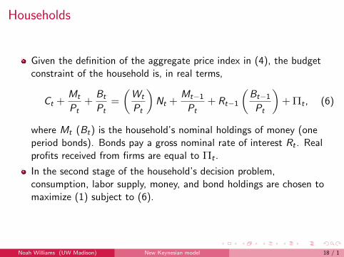
Given the definition of the aggregate price index in (4), the budgetconstraint of the household is, in real terms,

Ct +Mt

Pt+

Bt

Pt=

(Wt

Pt

)Nt +

Mt−1Pt

+ Rt−1

(Bt−1Pt

)+ Πt , (6)

where Mt (Bt) is the household’s nominal holdings of money (oneperiod bonds). Bonds pay a gross nominal rate of interest Rt . Realprofits received from firms are equal to Πt .

In the second stage of the household’s decision problem,consumption, labor supply, money, and bond holdings are chosen tomaximize (1) subject to (6).


Households

The following conditions must also hold in equilibrium

1 the Euler condition for the optimal intertemporal allocation ofconsumption

C−σt = βRtEt

(Pt

Pt+1

)C−σ;t+1 (7)

2 the condition for optimal money holdings:

γ(MtPt

)−bC−σt

=Rt − 1

Rt; (8)

3 the condition for optimal labor supply:

χNηt

C−σt

=Wt

Pt. (9)


Firms

Firms maximize profits, subject to three constraints:

1 The first is the production function summarizing the technologyavailable for production. For simplicity, we have ignored capital, sooutput is a function solely of labor input Njt and an aggregateproductivity disturbance Zt :

cjt = ZtNjt , E(Zt) = 1.

2 The second constraint on the firm is the demand curve each faces.This is given by equation (5).

3 The third constraint is that each period some firms are not able toadjust their price. The specific model of price stickiness we will use isdue to Calvo (1983).


Price adjustment

Each period, the firms that adjust their price are randomly selected: afraction 1−ω of all firms adjust while the remaining ω fraction donot adjust.

I The parameter ω is a measure of the degree of nominal rigidity; alarger ω implies fewer firms adjust each period and the expected timebetween price changes is longer.

For those firms who do adjust their price at time t, they do so tomaximize the expected discounted value of current and future profits.

I Profits at some future date t + s are affected by the choice of price attime t only if the firm has not received another opportunity to adjustbetween t and t + s. The probability of this is ωs .


Price adjustmentThe firm’s decision problem

First consider the firm’s cost minimization problem, which involvesminimizing WtNjt subject to producing cjt = ZtNjt . This problem canbe written as

minNt

WtNt + ϕnt (cjt − ZtNjt) .

where ϕnt is equal to the firm’s nominal marginal cost. The first order

condition impliesWt = ϕn

tZt ,

or ϕnt = Wt/Zt . Dividing by Pt yields real marginal cost as

ϕt = Wt/ (PtZt).


Price adjustmentThe firm’s decision problem

The firm’s pricing decision problem then involves picking pjt tomaximize

Et

∞

∑i=0

ωi∆i ,t+iΠ(

pjtPt+i

, ϕt+i , ct+i

)=

Et

∞

∑i=0

ωi∆i ,t+i

[(pjtPt+i

)1−θ

− ϕt+i

(pjtPt+i

)−θ]Ct+i ,

where the discount factor ∆i ,t+i is given by βi (Ct+i/Ct)−σ andprofits are

Π(pjt) =

[(pjtPt+i

)cjt+i − ϕt+icjt+i

]


Price adjustment

All firms adjusting in period t face the same problem, so all adjustingfirms will set the same price.

Let p∗t be the optimal price chosen by all firms adjusting at time t.The first order condition for the optimal choice of p∗t is

Et

∞

∑i=0

ωi∆i ,t+i

[(1− θ)

(1

pjt

)(p∗tPt+i

)1−θ

+ θϕt+i

(1

p∗t

)(p∗tPt+i

)−θ]Ct+i = 0.

Using the definition of ∆i ,t+i ,

(p∗tPt

)=

(θ

θ − 1

) Et ∑∞i=0 ωi βiC 1−σ

t+i ϕt+i

(Pt+i

Pt

)θ

Et ∑∞i=0 ωi βiC 1−σ

t+i

(Pt+i

Pt

)θ−1 . (10)


The case of flexible prices

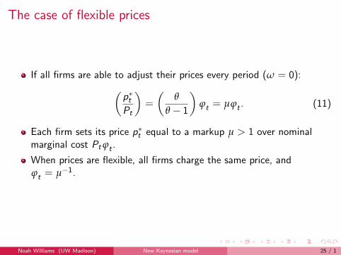
If all firms are able to adjust their prices every period (ω = 0):(p∗tPt

)=

(θ

θ − 1

)ϕt = µϕt . (11)

Each firm sets its price p∗t equal to a markup µ > 1 over nominalmarginal cost Pt ϕt .

When prices are flexible, all firms charge the same price, andϕt = µ−1.


The case of flexible prices

Using the definition of real marginal cost, this means

Wt

Pt=

Zt

µ.

However, the real wage must also equal the marginal rate ofsubstitution between leisure and consumption to be consist withhousehold optimization:

χNηt

C−σt

=Zt

µ. (12)


The case of flexible pricesFlexible-price output

Let a xt denote the percent deviation of a variable Xt around itssteady-state. Then, the steady-state yields

ηnt + σct = zt .

Now using the fact that yt = nt + zt and yt = ct , flexible-priceequilibrium output y ft can be expressed as

y ft =

[1 + η

η + σ

]zt . (13)


The case of sticky prices

When prices are sticky (ω > 0), the firm must take into accountexpected future marginal cost as well as current marginal cost whensetting p∗t .

The aggregate price index is an average of the price charged by thefraction 1−ω of firms setting their price in period t and the averageof the remaining fraction ω of all firms who set prices in earlierperiods.

Because the adjusting firms were selected randomly from among allfirms, the average price of the non-adjusters is just the average priceof all firms that was prevailing in period t − 1.

Thus, the average price in period t satisfies

P1−θt = (1−ω)(p∗t )

1−θ + ωP1−θt−1 . (14)


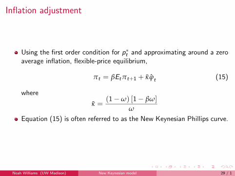
Inflation adjustment

Using the first order condition for p∗t and approximating around a zeroaverage inflation, flexible-price equilibrium,

πt = βEtπt+1 + κ ϕt (15)

where

κ =(1−ω) [1− βω]

ω

Equation (15) is often referred to as the New Keynesian Phillips curve.


Forward-looking inflation adjustment

The New Keynesian Phillips curve is forward-looking; when a firm setsits price, it must be concerned with inflation in the future because itmay be unable to adjust its price for several periods.

Solving forward,

πt = κ∞

∑i=0

βiEt ϕt+i ,

Inflation is a function of the present discounted value of current andfuture real marginal cost.

Inflation depends on real marginal cost and not directly on a measureof the gap between actual output and some measure of potentialoutput or on a measure of unemployment relative to the natural rate,as is typical in traditional Phillips curves.


Real marginal cost and the output gap

The firm’s real marginal cost is equal to the real wage it faces dividedby the marginal product of labor: ϕt = Wt/PtZt .

Because nominal wages have been assumed to be completely flexible,the real wage must equal the marginal rate of substitution betweenleisure and consumption.

In a flexible price equilibrium, all firms set the same price, so (11)implies that ϕ = µ−1. From equation (9), wt − pt = ηnt + σytRecalling that ct = yt , yt = nt + zt , the percentage deviation of realmarginal cost around the flexible price equilibrium is

ϕt = [ηnt + σyt ]− zt = (η + σ)

[yt −

(1 + η

η + σ

)zt

].


Real marginal cost and the output gap

But from (13), this can be written as

ϕt = (η + σ)(yt − y ft

). (16)

Using these results, the inflation adjustment equation (15) becomes

πt = βEtπt+1 + κxt (17)

where κ = (η + σ) κ = (η + σ) (1−ω) [1− βω] /ω andxt ≡ yt − y ft is the gap between actual output and the flexible-priceequilibrium output.

This inflation adjustment or forward-looking Phillips curve relatesoutput, in the form of the deviation around the level of output thatwould occur in the absence of nominal price rigidity, to inflation.


The demand side of the model

Start with Euler condition for optimal consumption choice

C−σt = βRtEt

(Pt

Pt+1

)C−σt+1

Linearize around steady-state:

−σct = (ıt − Etpt+1 + pt)− σEt ct+1

or

ct = Et ct+1 −(

1

σ

)(ıt − Etpt+1 + pt) .

Goods market equilibrium (no capital)

Yt = Ct .


The demand side of the modelLinearization

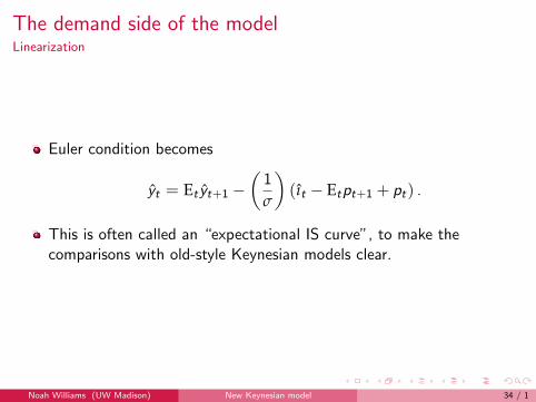
Euler condition becomes

yt = Et yt+1 −(

1

σ

)(ıt − Etpt+1 + pt) .

This is often called an “expectational IS curve”, to make thecomparisons with old-style Keynesian models clear.


Demand and the output gap

Express in terms of the output gap xt = yt − y ft :

yt − y ft = Et

(yt+1 − y ft+1

)−(

1

σ

)(ıt − Etpt+1 + pt)+

(Et y

ft+1 − y ft

),

or

xt = Etxt+1 −(

1

σ

)(rt − rnt ) ,

where rt = ıt − Etpt+1 + pt and

rnt ≡ σ(

Et yft+1 − y ft

).

Notice that the nominal interest rate affects output through theinterest rate gap rt − rnt .


The general equilibrium model

Two equation system

πt = βEtπt+1 + κxt

xt = Etxt+1 −(

1

σ

)(ıt − Etπt+1 − rnt )


The general equilibrium model

Consistent with

I optimizing behavior by households and firmsI budget constraintsI market equilibrium

Two equations but three unknowns: xt , πt , and it – need to specifymonetary policy


Documents

The New Keynesian Model - SSCCnwilliam/Econ714_files/... · The New Keynesian Model ... (3.3) 10.0 (3.3) ... The basic model of monopolistic competition is drawn from Dixit and Stiglitz