The New Generation Gap Economist Division of Consumer ... 2005 and 2015. 9 —U.S. BUREAU OF LABOR STATISTICS ... “Luxury” component. 26 —U.S. BUREAU OF LABOR STATISTICS

1 — U.S. BUREAU OF LABOR STATISTICS • bls.gov

Comparing Economic Status of Pre-Recession Millennialsto Post-Recession ‘September 11ths’

(Preliminary Analysis)

The New Generation Gap:

Geoffrey Paulin, Ph.D.Senior Economist

Division of Consumer Expenditure SurveysAmerican Council on Consumer Interests

April 23, 2017Albuquerque, NM

2 — U.S. BUREAU OF LABOR STATISTICS • bls.gov2 — U.S. BUREAU OF LABOR STATISTICS • bls.gov

The work in progress described herein requires Consumer Expenditure Survey (CE)

microdata to complete…


…However, tabular data provide a basis for preliminary analysis.


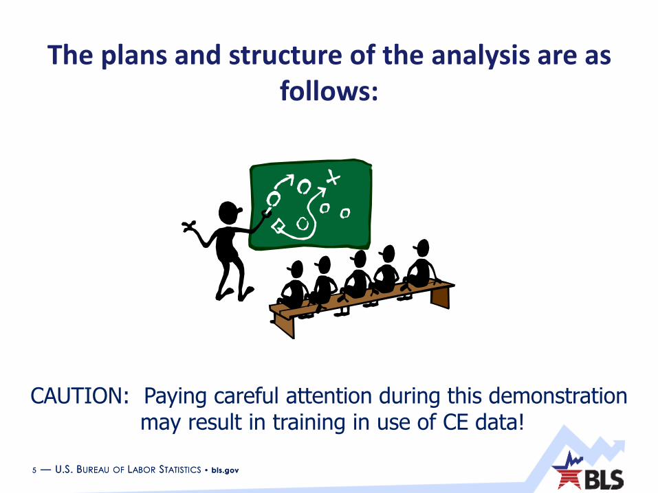
The plans and structure of the analysis are as follows:

CAUTION: Paying careful attention during this demonstrationmay result in training in use of CE data!


Background

Basic question: Are young adults “better off” today than were their counterparts 10 years ago (before/after the recession)?

This is an update in a continuing series exploring this question.

“Early” boomers, “late” boomers, and Generation X;

Late boomers and late Generation X/early Millennials

The youngest and oldest consumers before, during, and after the recent recession (forthcoming)


Tools for Preliminary Analysis

Tabular Data: Selected Age of Reference Person,2005 and 2015


Demographic differences head the tables.

The number of “young adult” consumer units falls more than 2 percent, while the rest of the population grows by 12 percent! Is this due to:

Actual population decline (“baby bust”); or

Young adults returning home after (or never leaving for) college?

Only the Census Bureau knows for sure!*

Homeownership rates are noticeably lower (5 to 6 percentage points) for each group in 2015 than 2005.

Hispanics account for larger percentages (2 to 3 points) of each group in 2015.

*Actually, so do CE Microdata, but remember, this work describes tabular data only.


Changes in Real Income

Ingredients:

Nominal incomes in 2005 and 2015

Value of the Consumer Price Index (CPI) in 2005 and 2015

Source: BLS Websites

CE data: https://www.bls.gov/cex/tables.htm (Selected age of reference person, XLSX format)

CPI data: https://www.bls.gov/cpi/home.htm (Multi-screen data search tool for all urban consumers, current series)


First, compute the CPI adjustment factor:

CPI 2005: 195.3

CPI 2015: 237.017*

Adjustment factor: (237.017/195.3) = 1.214

*CPI started publishing values to three decimal places in January 2007.


After applying the adjustment factor, the following is noted:

Real ($ 2015) Income before taxes 2005 2015 Percent change

Under 30 $46,392 $46,130 -0.6%

30 and over $75,841 $73,417 -5.3%

Incomes have fallen for young adults;but much more for those who are older!


However, “permanent” incomes (proxied by total expenditures) are different:

Real ($ 2015) Average Annual Expenditures 2005 2015 Percent change

Under 30 $41,903 $40,761 -2.7%

30 and over $58,980 $58,463 -1.3%

The percent decline in permanent incomes foryoung adults is twice the rate of those who are older.


Aggregate Shares

1. Compute aggregate dollars for which each group accounts. (E.g., how many billions of dollars did young adults spend on Good X in 2005, and in 2015?)

2. Compute the aggregate share of interest in each time period (i.e., the proportion of TOTAL billions of dollars spent on Good X in each year for which young adults account).

3. Compute the portion of the population for which young adults account.

4. Compare the aggregate share to the population share to see if young adults consistently “over” or “under” spend their share.


Computing Aggregate Shares

Ingredients:

Average annual expenditures (or income) in 2005 and 2015

– Young adults (under 30)

– Older adults (30 and older)

Total numbers of consumer units by each age group in 2005 and 2015

Source: Selected Age of Reference Person table


Example:Consumer Units (CUs) in 2005

Young adults: 18,282,000 (18.2 million)

Older adults: 99,074,000 (99.1 million)

Total population: 117,356,000 (117.4 million)

Average annual food expenditures in 2005

Young adults: $4,564

Older adults: $6,182

Aggregate Expenditure:

Young adults: $83.4 billion ($4,564*18.2 million)

Older adults: $612.5 billion ($6,182*99.1 million)

Total population: $695.9 billion ([$83.4 plus $612.5] billion)


Comparing Population and Aggregate Share: Young Adults

Population share: 15.6 percent

18.2 million (young adult CUs) / 117.4 million (total population CUs)

Aggregate food expenditure share: 12.0 percent

$83.4 billion (aggregate young adult expenditure)

$695.9 billion (aggregate expenditure for total population

$83.4 billion / $695.9 billion = 12.0 percent

Finding: Young adults “underspend” their share (12.0 < 15.6)


The results are similar for this group in 2015:

Population share: 13.9 percent

Aggregate food expenditure share: 10.9 percent


Possible Explanations:

Family Size?

No. Consider Average CU size (in 2005):

– Under 30: 2.3

– 30 and over: 2.5

Income?

Could be.

– Under 30: $38,227 (2005)

– 30 and over: $62,492 (2005)

– Gap is similar in 2015 ($46,130 vs. $73,417)

Other factors?

Indeterminate. Requires microdata for regression analysis.


Next, consider Engel’s Proposition.

I SAID “ENGEL’S PROPOSITION,”

NOT “ANGLES, PREPOSITION!”

Of


Syllogistic Reasoning:

Engel’s Finding (1857): The larger the income, the smaller the share allocated to food.

Axiom: The smaller the share allocated to food, the more “left over” for other spending.

Conclusion: Smaller food shares indicate higher social welfare/economic status.


Note that “Food” has two components:

Food at home

Food purchased at grocery stores and similar outlets

“Necessity” component

Food away from home

Food purchased from restaurants and similar establishments

“Luxury” component


Results for Food at Home:

Under 30 2005 2015

Food (H) $2,291 $2,830

Total Exps. $34,528 $40,761

Share 7.1% 7.2%

30/older 2005 2015

Food (H) $3,481 4,217

Total Exps. $48,599 $58,463

Share 6.6% 6.9%

By this measure, young adults have no change in status, while their elders are slightly “worse off.”


Similarly, one can examine “budget shares”:

Total Food = Food at Home + Food Away from home.

How much of the total food budget is allocated to:

Food at home (“necessity” share)

Food away from home (“luxury” share)


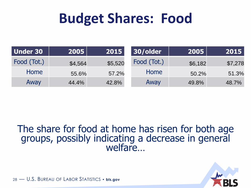
Budget Shares: Food

Under 30 2005 2015

Food (Tot.) $4,564 $5,520

Home 55.6% 57.2%

Away 44.4% 42.8%

30/older 2005 2015

Food (Tot.) $6,182 $7,278

Home 50.2% 51.3%

Away 49.8% 48.7%

The share for food at home has risen for both age groups, possibly indicating a decrease in general

welfare…


…However:

Other possibilities, such as changes in relative prices of food at and away from home, have not yet been examined.

Note that CPI has information on both, available online. (At site cited earlier.)

Also note that expenditures for total food are “nominal.” (The CPI-all adjustment factor would have cancelled out anyway.)


Of major interest during this period is housing.

The “housing bubble” famously burst in or around 2007.

CE data show changes in both:

Spending for owned and rented dwellings before and after this period

Changes in housing tenure, as noted at the beginning of this segment.


Especially because of changing tenure, the analysis is complicated.

Housing expenditures are averaged over ALL consumers.

That is, they represent expenditures as if the “average consumer” is (generally) 60 percent homeowner and 40 percent renter.

At any given time, most consumers are one or the other, not both.


To properly compare across tenures and time:

Examine owned dwelling expenditures separately from rented dwelling expenditures.

Divide owned dwelling expenditures by percent homeowners. This produces an estimated average expenditure on owned dwellings for those who own.

Repeat for renters (substituting “rent” for “own” of course).


While not yet completed for this analysis….

…I hope you will read the paper when it appears in print.


This concludes your introduction to the Selected Age of Reference

Person CE tabular data.

Contact Information


Geoffrey Paulin, Ph.D.Senior Economist

Division of Consumer Expenditure Surveyswww.bls.gov/cex

[email protected]

Documents

The New Generation Gap Economist Division of Consumer ... 2005 and 2015. 9 —U.S. BUREAU OF LABOR STATISTICS ... “Luxury” component. 26 —U.S. BUREAU OF LABOR STATISTICS