The Mundell-Fleming Model with Partial International

445

CHAPTER 22

The Mundell-Fleming Modelwith Partial InternationalCapital Mobility

This chapter adds international capital flows to the basic model, continuing theprocess of adding new factors one by one to our analysis of the balance of pay-ments. Chapter 16 examined the effects of changes in the exchange rate, holding

everything else constant. Then Chapter 17 introduced the level of income, and Chap-ter 18, the interest rate. Chapter 19 focused on international money flows and the price level.

In Chapter 21 we saw in detail that the degree of international capital mobility hasincreased steadily over the past 30 years. This chapter and those to follow will demon-strate that international capital mobility has important implications for the operationof macroeconomic policy. For example, the most dramatic shift of the 1980s in the eco-nomic interaction of the industrialized countries, the emergence of large trade deficitsin the United States, was not primarily caused by changes in trade policy or competi-tiveness. Rather, it had its origin in the international flow of capital to the UnitedStates.This flow of capital, in turn, was caused primarily by fiscal and monetary policiesenacted in Washington, D.C. An analogous shift in fiscal and monetary policies inGermany in the early 1990s had similar consequences for that country. In some waysthe United States is repeating the experiment in the current decade.

In reality, international capital flows depend on many factors. Perhaps the mostimportant are the rates of return that various countries are offering on their assets. Wewill simplify and assume that the rates of return on all assets offered by a given country(other than money) move together sufficiently closely within the country that they canbe represented by a single nominal interest rate, i. In other words, we aggregate togetherbonds, stocks, and other nonmonetary assets. It is further assumed here that the differ-ential between the domestic and foreign interest rate is the only determinant of the netcapital inflow or outflow. Chapters 27 and 28 will add other determinants of the behav-ior of the international portfolio investor besides interest rates: in particular, investors’awareness that future changes in exchange rates will affect the returns they earn.

When investors in a low-interest-rate country buy assets in a high-interest-ratecountry, they exploit the principle of comparative advantage, just as consumers do whenbuying goods from a foreign country that can produce them at lower cost. Chapters 2and 3 introduced the concept of autarky—the hypothetical situation that would prevail

CAVE.6607.cp22.p445-466 6/6/06 12:31 PM Page 445

if a country were closed off from international trade in goods (for example, because ofprohibitively high tariff barriers), so that agents could consume only those goods pro-duced domestically. It was shown that once the country opens up to international trade,the pattern of trade is dictated by the prices that would hold in autarky: If one good sellsfor a lower price in the foreign country than in the domestic country (whether becausedemand for it is lower or supply higher), then domestic residents will import that goodas soon as they have the opportunity.

A similar concept can be applied to international trade in bonds. Autarky nowwould prevail if a country were closed off from international trade in bonds, that is,from borrowing or lending abroad (for example, because of prohibitively high capitalcontrols). In autarky the interest rate in each country would be determined so as toequilibrate the supply and demand for bonds versus money. The last part of Chapter 18introduced monetary policy and the interest rate, i, into the model, but did not allowfor international capital flows. In Figure 18.7, for example, a high interest rate wasrequired for equilibrium in the home country. There had been an increase in govern-ment demand for funds that reduced total national saving, and thus drove up the inter-est rate and crowded out private investment. (Do not be concerned if your recollectionof the graph is hazy; it will be covered again momentarily.)

Imagine now that in autarky a lower interest rate prevails in the foreign country.Once the countries open up to international capital flows, the pattern of trade in bondsis dictated by the rates of return. If the home country has the higher interest rate, thendomestic residents will borrow from abroad, where the cost of funds is lower.Equivalently, foreign residents will lend to the home country, where the rate of returnis higher. Either way, the point is that capital flows from the low-interest-rate countryto the high-interest-rate country.1

We represent the net (private) capital account balance by KA. Thus

(22.1)

To the extent that the domestic interest rate, i, rises above the foreign rate, i*, foreigninvestors will find domestic assets more attractive than their own and will seek toacquire them; domestic residents will be less eager to buy foreign assets and may evenborrow abroad at the lower foreign interest rate. Whether foreigners invest in thehome country or domestic residents borrow abroad, the transaction counts as a capitalinflow and the domestic capital account shows a surplus: KA is positive. Conversely, ifthe domestic interest rate falls below the foreign rate, domestic residents will buy for-eign assets and foreign residents will borrow in the home country; there is a capital out-flow and KA is negative.

Why, if one country is offering a higher interest rate than another, would investorsbe willing to hold any assets of the low-rate country? This is a question well worth ask-ing, and there will be an answer to it that holds even under conditions of perfect inte-gration of financial markets (that is, the possibility of future changes in the exchange

KA 5 KA 1 k(i 2 i*)

446 Chapter 22 ■ The Mundell-Fleming Model with Partial International Capital Mobility

1To carry the analogy with the two-good trade model one step further, the “good” that the foreign countryobtains is the ability to consume more in the future in exchange for consumption today. This point was spelledout in Section 21.5.

CAVE.6607.cp22.p445-466 6/6/06 12:31 PM Page 446

rate, to be introduced in Chapter 27). For the moment, assume there are still sometransaction costs, capital controls, or other impediments to the movement of capitalacross national borders that prevent investors from completely arbitraging away inter-est differentials.2

This chapter inserts the capital flow equation, Equation 22.1, into the model usedto determine national income, Y, in Chapters 17 and 18. The chapter thus returns to theKeynesian assumption made there that the speed of adjustment of goods prices is soslow that it can be ignored in the short run, so that changes in demand are entirelyreflected as changes in output. (As before, much of the analysis developed here wouldalso apply in a world of flexible prices, with changes in the price level substituting forchanges in output when there are changes in aggregate demand.) Because Chapter 18assumed a capital account constrained to zero, the model did not look radically differ-ent from the IS-LM model of traditional closed-economy textbooks. Now, however,international capital flows will change the model radically, particularly regarding theeffects of monetary and fiscal policy.

In this chapter we hold the exchange rate constant. Then in Chapter 23 we con-sider a floating exchange rate regime. At every stage, the discussion explores not justwhat difference it makes to have some degree of capital mobility (k . 0) but also thedifferent implications of high versus low capital mobility. Section 23.3 will also considerthe limiting case of perfect capital mobility (k 5 infinity). This logical progression—from no capital mobility to low, high, and finally perfect capital mobility—mirrors thehistorical evolution of the international financial system as the processes of innovationand liberalization have gradually diminished the barriers between countries.

22.1 The Model

We set down equations for the IS and LM relationships from Chapter 18:

IS: Y = [ 2 b(i) 1 2 ] (s 1 m) (22.2)

LM: M P 5 L(i, Y) (22.3)

The curves appear in the figures used throughout this chapter.To review, the LM curve is the relationship between income, Y, and the interest

rate, i, that gives equilibrium in the money market, where equilibrium is defined as realmoney supply (M P) equal to real money demand. A given curve represents a givenreal money supply. The curve slopes upward because i and Y have opposite effects onmoney demand. An increase in Y raises the demand for money because people under-take more transactions. If there is no accommodating increase in the money supply,then the interest rate will be driven up, reducing the demand for money back to itsoriginal level. If the central bank adopts an expansionary monetary policy, under the

/

/

/ M X A

22.1 ■ The Model 447

2Again, to point out the analogy with trade in goods, the existence of transportation costs, tariffs, or otherimpediments to the movement of goods across national boundaries would prevent the prices for the identicalgoods from being equalized between the two countries.

CAVE.6607.cp22.p445-466 6/6/06 12:31 PM Page 447

assumption that the short-run price level is fixed, the increase in the nominal moneysupply is also an increase in the real money supply. It shifts the LM curve to the rightso that a higher level of Y can be sustained for any given interest rate.

The IS curve is the relationship between output, Y, and the interest rate, i, thatgives equilibrium in the goods market, where equilibrium is defined as a point wherethe amount of goods produced equals the amount of goods demanded. The curveslopes downward because i has a second role (in addition to the return paid to house-holds on nonmonetary assets). It is the cost to firms of borrowing funds to financeinvestment in plant and equipment or the cost to households of borrowing to financethe purchase of an automobile or other consumer durable. An increase in i reducessuch expenditures, and in turn (through the multiplier effect) leads to a lower level ofoutput throughout the economy. Just as the LM curve is drawn contingent on a givenlevel of the money supply, so too is the IS curve drawn contingent on a given level ofgovernment expenditure, G. G is subsumed in the intercept term for the equation,along with the exogenous components of consumer spending and business investment.An increase in any of these exogenous components of spending (D ) shifts the IScurve to the right by an amount equal to the simple Keynesian multiplier, which is DY 5 [1 (s 1 m)]D . Similarly, a reduction in the tax rate would leave householdswith more disposable income and would exogenously increase consumption. The mul-tiplier, 1 (s 1 m), is smaller than it would be if the economy were closed to interna-tional trade (1 s) because some of the spending leaks out into imports from abroad.The effect on income in complete IS-LM equilibrium is smaller still because the highertransaction demand for money drives up the interest rate and discourages investment.

The IS curve shifts to the right not only when there is an exogenous increase indemand for domestic goods coming from domestic residents (A), but also when there isan exogenous increase in demand for domestic goods coming from foreign residents,that is, when there is an increase in net exports (TB). This would be the case, for exam-ple, if there is a shift in foreign tastes toward domestic products or if quotas are imposedon imports. The same occurs if there is a devaluation (assuming the Marshall-Lernercondition is satisfied). It will often be necessary to take into account these sources ofshifts in the IS curve.

The Balance-of-Payments Relationship

In Chapter 18 a third line, labeled TB 5 0, was drawn. At that stage in the analysis thebalance of payments consisted solely of the trade balance because there was no capitalaccount.That can be considered the approximate situation of the world economy in the1950s, when capital flows were not free to respond to rates of return. (This is not to saythat the capital account was literally zero. There was an exogenous component, .)The interest rate had no effect on the balance of payments, so the line representingthe balance of payments was vertical: A unique level of income Y was consistent withbalance-of-payments equilibrium. Any point to the right was a point of deficit becausehigher income means higher imports, and any point to the left a point of surplus becauselower income means lower imports. The position of this line, however, like the position

KA

//

A/

A


CAVE.6607.cp22.p445-466 6/6/06 12:31 PM Page 448

22.1 ■ The Model 449

of the IS curve, shifts to the right when there is a change in the exchange rate. Somepoints that previously represented a trade deficit now represent a trade surplus.

In this chapter the third line, which we will now call the BP line, still representsequilibrium in the overall balance of payments, but this no longer means the trade bal-ance alone. It includes both the trade balance, TB, which depends negatively onincome and positively on the exchange rate as before, and the capital account, KA,which depends positively on the interest differential (i 2 i*) as in Equation 22.1:

BP 5 TB 1 KA 5 0

BP 5 2 2 mY 1 1 k(i 2 i*) 5 0. (22.4)

The third line represents combinations of income and the interest rate that wouldgive an overall balance of payments equal to zero. To help graph it on the same dia-gram as the IS and LM curves, we can solve the equation to show the level of the inter-est differential that corresponds to any given level of income, Y:

i 2 5 2(1 k)( 2 1 ) 1 (m k)Y. (22.5)

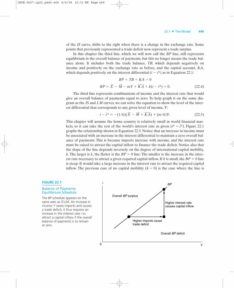
This chapter will assume the home country is relatively small in world financial mar-kets, so it can take the rest of the world’s interest rate as given (i* 5 *). Figure 22.1graphs the relationship shown in Equation 22.5. Notice that an increase in income mustbe associated with an increase in the interest differential to maintain a zero overall bal-ance of payments. This is because imports increase with income, and the interest ratemust be raised to attract the capital inflow to finance the trade deficit. Notice also thatthe slope of the line depends inversely on the degree of international capital mobility,k. The larger is k, the flatter is the BP 5 0 line: The smaller is the increase in the inter-est rate necessary to attract a given required capital inflow. If k is small, the BP 5 0 lineis steep: It would take a large increase in the interest rate to attract the required capitalinflow. The previous case of no capital mobility (k 5 0) is the case where the line is

i

/KA M X/i*

KA M X

FIGURE 22.1

Balance of PaymentsEquilibrium Schedule

The BP schedule appears on thesame axes as IS-LM. An increase inincome Y raises imports and causesa trade deficit; it thus requires anincrease in the interest rate i toattract a capital inflow if the overallbalance of payments is to remain at zero.

BP

Overall BP deficit

Overall BP surplus

Higher imports causetrade deficit

Higher interest ratecauses capital inflow

i

Y0

CAVE.6607.cp22.p445-466 6/6/06 12:31 PM Page 449

vertical: No finite increase in the interest rate would be enough to attract the capital.The slope also depends positively on the marginal propensity to import, m.3

Notice also that an increase in the exchange rate, or anything else that exoge-nously increases the trade balance, still shifts the BP curve to the right: For any giveninterest rate, the condition that the balance of payments is zero would now permit ahigher level of income. (The BP curve shifts to the right by precisely the same distanceas it did in the absence of capital mobility: (1 m)D .)

The economy is always at the intersection of the IS and LM curves, under theassumption that there is always equilibrium in the goods and asset markets.The demandfor goods equals the output of goods supplied, and the demand for money equalsthe supply of money.There is not necessarily any reason to be also on the BP curve.Thebalance of payments will be nonzero, and the economy will be off the BP curve, if thecentral bank is buying or selling foreign exchange reserves. The following discussionassumes that the starting point just happens to be a point where the balance of pay-ments equals zero, so all three curves intersect.

We now use the model to examine the effects, first, of a fiscal expansion and, sec-ond, of a monetary expansion.

22.2 Fiscal Policy and the Degree of Capital Mobility Under Fixed Rates

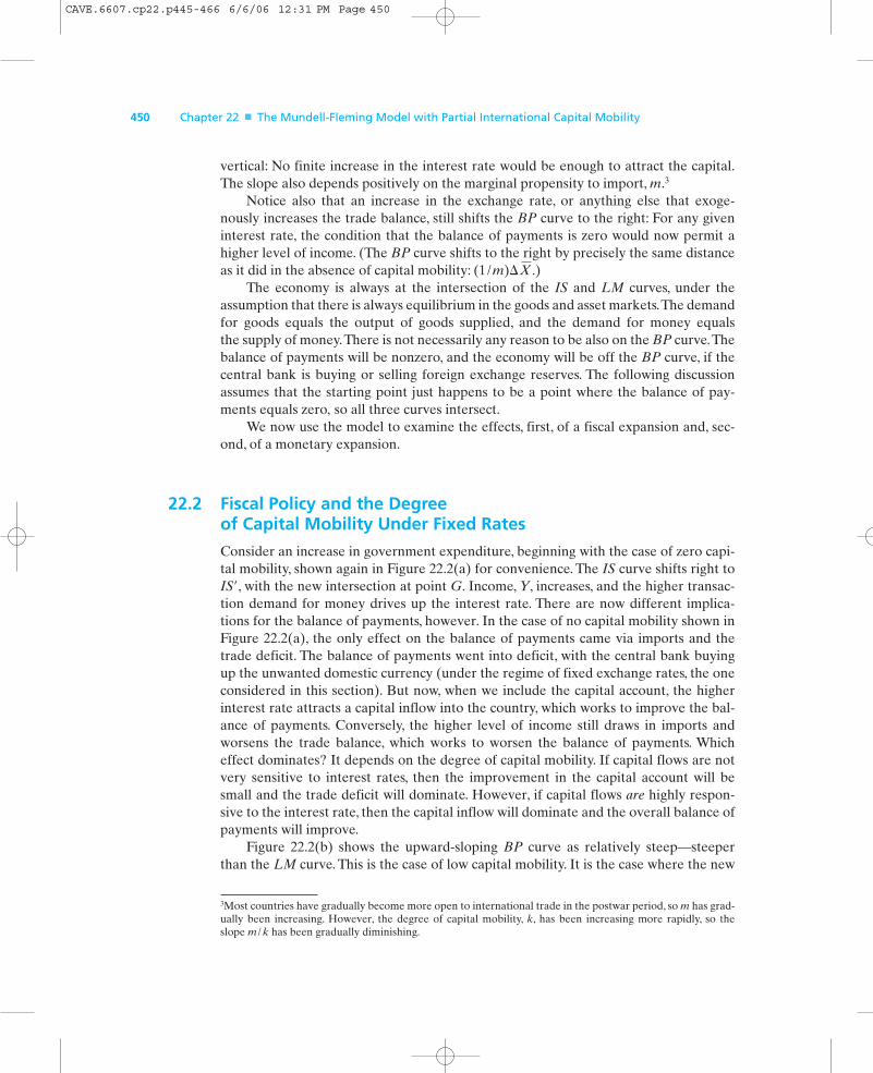
Consider an increase in government expenditure, beginning with the case of zero capi-tal mobility, shown again in Figure 22.2(a) for convenience. The IS curve shifts right toIS9, with the new intersection at point G. Income, Y, increases, and the higher transac-tion demand for money drives up the interest rate. There are now different implica-tions for the balance of payments, however. In the case of no capital mobility shown inFigure 22.2(a), the only effect on the balance of payments came via imports and thetrade deficit. The balance of payments went into deficit, with the central bank buyingup the unwanted domestic currency (under the regime of fixed exchange rates, the oneconsidered in this section). But now, when we include the capital account, the higherinterest rate attracts a capital inflow into the country, which works to improve the bal-ance of payments. Conversely, the higher level of income still draws in imports andworsens the trade balance, which works to worsen the balance of payments. Whicheffect dominates? It depends on the degree of capital mobility. If capital flows are notvery sensitive to interest rates, then the improvement in the capital account will besmall and the trade deficit will dominate. However, if capital flows are highly respon-sive to the interest rate, then the capital inflow will dominate and the overall balance ofpayments will improve.

Figure 22.2(b) shows the upward-sloping BP curve as relatively steep—steeperthan the LM curve. This is the case of low capital mobility. It is the case where the new

X/


3Most countries have gradually become more open to international trade in the postwar period, so m has grad-ually been increasing. However, the degree of capital mobility, k, has been increasing more rapidly, so theslope m k has been gradually diminishing./

CAVE.6607.cp22.p445-466 6/6/06 12:31 PM Page 450

IS-LM intersection at point G occurs to the right of or below the BP curve. Any pointto the right of or below the BP curve is a point of deficit: Either the level of income,and therefore imports, is too high for balance-of-payments equilibrium, or the level ofthe interest rate, and therefore the capital inflow, is too low. Thus the fiscal expansionin Figure 22.2(b) gives a balance-of-payments deficit, as in the case of zero capitalmobility, with the central bank buying up the unwanted domestic currency on theforeign exchange market. Yet there is a difference: The deficit is not as large as in Fig-ure 22.2(a) because the capital inflow does partially offset the trade deficit. This is theonly difference. Y and i are the same as in the earlier case.

In Figure 22.2(c) the BP curve is relatively flat—flatter than the LM curve. This isthe case of high capital mobility. The fiscal expansion again produces the sameincreases in Y and i. Now, however, the new intersection of the IS and LM curvesoccurs at a point, G, to the left of or above the BP curve. The increase in i attracts acapital inflow more than sufficient to finance the higher imports resulting from theincrease in Y. Thus the overall balance of payments is in surplus. Under fixed exchangerates, the central bank is accumulating foreign exchange reserves, not losing them, aswith a lower degree of capital mobility.

Which case, (a), (b), or (c), is most realistic in practice? Clearly, all countries haveat least some degree of capital mobility. The degree of capital mobility for the UnitedStates and Canada has been high enough to put them in category (c) ever since capital

22.2 ■ Fiscal Policy and the Degree of Mobility Under Fixed Rates 451

FIGURE 22.2

Fiscal Expansion Under Fixed Exchange Rates

(a) Regardless of the degree of capital mobility, a fiscal expansion shifts the IS curve out, raising Yand i at G and worsening the TB. If capital mobility is low (b), then the capital inflow, KA, is smallerthan the trade deficit and the overall BP is negative. If it is high (c), then KA is larger than the tradedeficit and BP is positive.

BP

L

G

IS ′ IS ′ IS ′

IS

TB

LM

(a) Zero Capital Mobility

i

Y0

BP

L

G

IS

TB

LM

(b) Low Capital Mobility

i

Y0

+KA

= BP

BPL

G

IS

LM

(c) High Capital Mobility

i

Y0

TB

+KA

= BP

CAVE.6607.cp22.p445-466 6/6/06 12:31 PM Page 451

controls were removed in 1974. Still, many other countries have lagged behind in liber-alizing their financial markets, as we noted in Chapter 21. The United Kingdom wasstill in category (b) in 1978, and Japan in 1984. By now, these countries are in category(c). None is on fixed exchange rates, so the complete analysis relevant to them willhave to await Chapter 23, which deals with floating rates.

Nevertheless, many continental European countries have tried to maintain fixedexchange rates against each other—first, starting in 1979, as part of the EuropeanMonetary System (EMS). Since 1999 many have locked their currencies together per-manently, in the EMU. So this analysis can be applied to them. Consider the exampleof France, which undertook an expansion when the socialists were elected in 1981. Atthe time, capital controls placed the country in category (b). The balance of paymentswent into deficit, so the French franc was in excess supply (vis-à-vis the German mark)and President Mitterrand was forced to reverse the expansion. In other words, Francehad difficulty attracting the foreign capital to finance fiscal expansion.

Subsequently, liberalization moved France from category (b) to category (c), wheremost Western European countries are now. Deficits are easily financed. Germany in1991–1992 undertook quite a large increase in government spending in an effort torebuild the economies of the newly reincorporated Eastern länder.The macroeconomiceffect was to push interest rates up sharply, which attracted a large capital inflow intoGermany and put strong upward pressure on the mark.

Fixed exchange rates are common in small developing countries. However, smallcountries usually have a high marginal propensity to import, so a fiscal expansion leadsto a large trade deficit. Most developing countries naturally have less developed finan-cial markets. As a result, interest rates may not be free to rise in response to a fiscalexpansion. Even if interest rates do rise above the level in the rest of the world, thedegree of capital mobility is likely to be low enough that the overall balance of pay-ments worsens rather than improves. In other words, they are in case (b).

This analysis has assumed that the central bank holds the money supply constant.The effect of the fiscal expansion would be greater if the central bank at the same timewere to follow an expansionary, or “accommodating,” monetary policy so as to preventinterest rates from rising. The Federal Reserve generally followed such a policy in the1960s when expansionary fiscal policies were adopted: the 1964 tax cut originally pro-posed by President Kennedy and the subsequent increases in spending by PresidentJohnson during the Vietnam era. We now consider the effects of an increase in themoney supply itself.

22.3 Monetary Policy and the Degree of Capital Mobility Under Fixed Rates

Figures 22.3(a), (b), and (c) again illustrate the cases of zero, low, and high capitalmobility, respectively. From the initial equilibrium, a monetary expansion shifts the LMcurve to the right. The effects of the increase in the money supply on the interest rateand income are precisely the same in each of the three cases. The interest rate, i, falls,stimulating spending and raising income, Y, to the new intersection point M. In each


CAVE.6607.cp22.p445-466 6/6/06 12:31 PM Page 452

case, higher income means higher imports and a trade deficit. However, the presence ofinternational capital mobility has implications for the balance of payments. This timethere is a capital outflow, resulting from the fact that i has fallen below the foreign rate,i*. Because the capital account moves in the same direction as the trade balance, theoverall balance of payments is in deficit in each of the three cases. Because the lowerinterest rate causes larger capital outflows at higher degrees of capital mobility, theoverall balance of payments must deteriorate by more in case (b) than in case (a), andby more in case (c) than in case (b).

If a country is running a balance-of-payments deficit, as in Figure 22.3(a), (b), and(c), it is losing foreign exchange reserves continuously over time. Because it has only acertain level of reserves, it cannot continue to do this indefinitely. Eventually, it mustadjust. One way would be deliberately reversing the monetary expansion. Yet there isalso the possibility of automatic adjustment of the money supply through the balance-of-payments deficit if the central bank does not sterilize reserve outflows. We considernonsterilized reserve flows momentarily.

A final way to adjust is to let the exchange rate change. A deliberate devaluationwould stimulate net exports and shift the BP curve to the right. The automatic versionof this mechanism of adjustment is to allow the currency to depreciate on the foreignexchange market, when the central bank follows a rule of not intervening, as we willsee in our discussion of floating exchange rates.

22.3 ■ Monetary Policy and the Degree of Capital Mobility Under Fixed Rates 453

FIGURE 22.3

Monetary Expansion Under Fixed Exchange Rates

(a) Regardless of the degree of capital mobility, a monetary expansion shifts the LM curve out,lowering i and raising Y at M, and worsening the TB. (b) With low capital mobility, an outflowthrough the KA supplements the trade deficit, so that the overall BP deficit and speed of reserveoutflow are greater. (c) With high capital mobility, the speed of reserve outflow is greater still.

BP

M IS

TB

LM

LM ′ LM ′ LM ′

(a) Zero Capital Mobility

i

Y0

BP

M IS

TB

LM

(b) Low Capital Mobility

i

Y0

KA+

= BP= BP

BP

M IS

LM

(c) High Capital Mobility

i

Y0

TB

KA+

CAVE.6607.cp22.p445-466 6/6/06 12:31 PM Page 453

So far in this chapter, capital mobility has affected only the balance of payments,not income. However, under either of these two possible (automatic) mechanisms ofadjustment—reserve flows or exchange rate changes—the changes in the balance ofpayments already derived will, in turn, have implications for the level of income.

22.4 When Money Flows Are Not Sterilized

If the central bank does choose to sterilize reserve flows, the economy can remain atpoint M in Figure 22.3 or at point G in Figure 22.2 as long as the stock of reserves holdsout. Now, however, the analysis adopts the assumption of the monetary approach to thebalance of payments: Changes in the level of reserves are not sterilized and thus areallowed to be reflected one for one as changes in the level of the total money supply.The preceding analysis still explains what happens to income and the interest rate in theshort run, but now it is necessary to trace the implications of the money flow over time.

Monetary Expansion and the Capital-Account Offset

We begin by picking up the experiment where the central bank undertakes a deliberateincrease in domestic credit.The combination of a lower interest rate and higher level ofincome at point M is only a short-run equilibrium. Even without any capital mobility,as in Figure 22.3(a), the trade deficit at point M in itself implies that reserves are flow-ing out of the country over time. If the central bank does not choose to sterilize thisloss in reserves, then the money supply is decreasing, which means the LM curve isshifting back to the left over time. The sequence of intersections back along the IScurve is shown by the arrows in Figure 22.3(a). They bring to mind the principle illus-trated in Figure 19.1 where the monetary approach to the balance of payments wasfirst encountered. As the money supply falls, the interest rate rises, discouraging busi-ness investment and other interest-sensitive components of spending.This process con-tinues as long as the balance of payments is still in deficit. In the long run, the economyis back where it started. The entire increase in the money supply has flowed outthrough the balance of payments, leaving no permanent effect on income.

The story is similar when we add some degree of capital mobility as in Fig-ure 22.3(b). Because the lower interest rate induces a deficit on the capital account aswell, the overall balance of payments at point M is in greater deficit than it was in theabsence of capital mobility. As in the case without capital mobility, if the central bankopts not to sterilize the reserve outflow, then the economy follows the sequence ofarrows until in the long run it is back where it started, with no effects. Is this case thenidentical to the case illustrated in Figure 22.3(a)? The two graphs look quite similar,but there is a difference. Because the balance-of-payments deficit is greater in the caseof capital mobility illustrated in Figure 22.3(b), the rate at which the money supplydecreases over time is greater, and therefore the economy returns to its starting pointmore rapidly.

The case of high capital mobility, illustrated in Figure 22.3(c), proceeds in the sameway. The balance-of-payments deficit at point M means that the addition to the money


CAVE.6607.cp22.p445-466 6/6/06 12:31 PM Page 454

supply is flowing out of the country over time. In the long run the economy is againback where it started. What difference does the higher degree of capital mobilitymake? Because the capital outflow is greater for the same differential in interest rates,the rate of reserve loss is even greater in Figure 22.3(c) than in Figure 22.3(b), and sothe return to the long-run equilibrium will be that much faster. The speed with whichincreases in domestic credit flow out through the capital account is called the speed of offset.

Fiscal Expansion and Capital Mobility

We now turn from the experiment where the government undertakes a deliberatemonetary expansion to the experiment where it undertakes a deliberate fiscal expan-sion, such as an increase in government expenditure. Figure 22.2 showed an outwardshift in the IS curve and an increase in income. Recall that the higher level of incomeresulted in a trade deficit, just as in the monetary expansion.

When a fiscal expansion results in a balance-of-payments deficit, the money sup-ply will gradually decrease over time if the central bank does not sterilize the reserveoutflow. The declining money supply will shift the LM curve leftward and the interestrate will rise. We now move up the new IS curve (IS9) in a sequence of IS-LM intersec-tions, with interest-sensitive expenditures declining. As expenditure declines, the tradebalance improves. This process continues until the economy has returned to a zero bal-ance of payments. Only then are we in long-run equilibrium, because only then is themoney supply no longer changing. The arrow in Figure 22.2(a) shows this process for the case of zero capital mobility and reminds us of the lesson learned from Fig-ure 19.B.1: In the long run (point L), the fiscal expansion is completely offset by theoutflow of money and there is no effect on the level of output. In the case of low capi-tal mobility illustrated in Figure 22.2(b), the balance-of-payments deficit that exists atpoint G again means that reserves will be flowing out over time and that under thenonsterilization assumption the money supply and level of income will be decliningover time. In this case, however, the long-run equilibrium at point L features a level ofincome that, although below the short-run level at point G, is still somewhat higherthan before the fiscal expansion.

What about the case of high capital mobility, illustrated in Figure 22.2(c)? We have already seen that the short-run equilibrium at point G is a point of balance-of-payments surplus, rather than deficit. The capital inflow is more than enough to offsetthe trade deficit. This represents a qualitative departure from the other five cases illus-trated. It means that the stock of international reserves is increasing over time, notdecreasing. If the central bank opts not to sterilize, but rather allows the total moneysupply to increase over time, then the LM curve will again shift, but to the right thistime. From point G, the economy moves to the right along the IS9 curve, with thehigher money supply driving down the interest rate and stimulating spending. Thelong-run equilibrium occurs at L, where the capital inflow is no more than is needed tofinance the trade deficit. Unlike the case with low capital mobility, the level of incomein the long run is not just higher than it was before the fiscal expansion, it is also higherthan in the short run.

22.4 ■ When Money Flows Are Not Sterilized 455

CAVE.6607.cp22.p445-466 6/6/06 12:31 PM Page 455

Are Capital Flows and Money Flows the Same Thing?

It is appropriate here to note a pitfall that may be encountered when analyzing inter-national money flows. A capital inflow, such as that resulting from the increase in inter-est rates shown in Figure 22.2, is sometimes referred to as an “inflow of money.” This is permissible terminology because foreign residents are usually paying for the stocksand bonds they buy with money. However, it is important to realize that at the sametime that money is “flowing in” through the capital account, it may be “flowing out”through the trade account. It takes money to buy goods, just as it takes money to buysecurities. Money is only truly flowing in, on net, if the total balance of payments is insurplus—that is, both the trade account and the capital account—as in the short-runequilibrium at point G in Figure 22.2(c). Even then, the total money supply does notincrease unless the central bank allows it to, by refraining from sterilizing the inflow. Itis probably safest to avoid altogether using the term inflow of money to describe aninflow of capital. Then there will be no danger of confusing it with a change in themoney supply. There are many other more suitable synonyms for capital inflow tochoose from (borrowing from abroad, foreign financing, foreign investment in thedomestic country, decrease in the net international investment position, foreign pur-chases of domestic assets, etc.).

As we have seen repeatedly, under the monetary approach to the balance of pay-ments, the overall balance is zero in the long run. At point L in Figure 22.2, however,there must be a continuing capital inflow because the domestic interest rate remainsabove the world interest rate. “Money” is flowing in through the capital account at pre-cisely the same rate as it is flowing out through the current account. Another implica-tion is that in the long run all three curves intersect (at the same point L), not just theIS and LM curves.

22.5 Other Automatic Mechanisms of Adjustment

Within the context of the monetary approach to the balance of payments, the findingsof Figure 22.2(b) and (c) are unfamiliar.As a general rule, it is expected that in the longrun, when the economy has had enough time to adjust to a change in macroeconomicpolicy, there are no real effects left. Yet it has just been shown that under conditions ofcapital mobility, a fiscal expansion seems to have a permanent effect on real output. Itis clear why some effect on output can remain even in the long run in this model: Theonly automatic mechanism of adjustment is the flow of money through the balance ofpayments, which is shut off at point L. However, there are other automatic mechanismsof adjustment that have been omitted here.

One is the adjustment of the price level over time in response to an excess demandfor goods and labor. Inflationary pressure may exist at points like G in Figure 22.2 orM in Figure 22.3, assuming that the starting point before the fiscal or monetary expan-sion was near the point at which the economy was at potential output and full employ-ment. Chapter 19 showed that an increase in the price level reduces the real moneysupply, which works to discourage expenditure and return the economy to its long-run


CAVE.6607.cp22.p445-466 6/6/06 12:31 PM Page 456

equilibrium. Chapter 26 will add the gradual adjustment of goods prices to the modelof this chapter.

Another possible automatic mechanism of adjustment omitted here is changes inthe stock of bonds. This point is particularly relevant in Figure 22.2(b) and 22.2(c). Atpoint L the government is still running a budget deficit and—as a consequence—thecountry is still running a current-account deficit, even though the capital inflow is largeenough to finance these deficits. When the government runs a budget deficit, the sup-ply of government bonds in the hands of the public increases over time, assuming thatthe deficit is not monetized (i.e., assuming that the bonds are not bought by the centralbank—which they are not, under the assumption that the central bank is holding themoney supply constant). Analogously, when the country runs a current-account deficit,the supply of foreign bonds in the hands of the public decreases over time. In otherwords, the public borrows, or runs down the asset position vis-à-vis foreigners that ithas accumulated in the past, to pay for its trade deficit.

The stock of bonds (i.e., the accumulated level of bonds issued, as opposed to theflow, i.e., the deficits), either domestic or foreign, has no role to play in the modeldeveloped in this chapter. However, there are possible effects left out of the model. Forexample, holdings of bonds, along with money and other assets, are a component of thewealth or net worth of households and thus have an effect on the level of spending. Ifspending declines at point L in Figure 22.2(c) because households are running downtheir holdings of foreign bonds at the rate of the current-account deficit, then the IScurve will shift back to the left, just as it does when there is any exogenous fall indomestic spending. The process may continue until the current account is back to zeroand the stock of bonds back to where it started. There is an analogy with the monetaryapproach to the balance of payments, in which the adjustment process continues untilthe overall balance of payments is back to zero and the money supply is back to whereit started. This added possible mechanism of adjustment will not be pursued here. Thediscussion, rather, is based on the model in which changes in the stock of bonds haveno effect, so that it does not matter whether it is changing over time or not.4

22.6 The Pursuit of Internal and External Balance

The last section of Chapter 18 introduced a fundamental principle of policy-making:To attain the two independent policy targets of internal balance (output equal to adesired level) and external balance (the trade balance at a desired level), at least twoindependent policy instruments are required. In Chapter 18 the two policy instrumentswere spending and the exchange rate. In this chapter we have been keeping theexchange rate fixed, ruling out one of the instruments. (Chapter 23 will return to thecase of flexible exchange rates.) A new policy instrument, the money supply, has been

22.6 ■ The Pursuit of Internal and External Balance 457

4These effects are modeled in the portfolio-balance approach. One statement of the approach under fixedexchange rates is Lance Girton and Dale Henderson, “Financial Capital Movements and Central BankBehavior in the Two-Country Short-Run Portfolio-Balance Model,” Journal of Monetary Economics (1976):33–61. Chapter 28 will explain the portfolio-balance approach in the context of floating exchange rates.

CAVE.6607.cp22.p445-466 6/6/06 12:31 PM Page 457

added, however, since the issue was last considered. Monetary and fiscal policy areeach thought of as domestic policy instruments. Will the two, used together, never-theless allow the two targets of external and internal balance to be attained simultane-ously? The answer turns out to be yes, but only because the model now allows forinternational capital movements.5

Figure 22.4 repeats the earlier depiction of the Mundell-Fleming model under fixedexchange rates but emphasizes the government’s objectives more explicitly.The verticalline labeled TB 5 0 marks the unique level of income that corresponds to a trade bal-ance of zero, a possible interpretation of the external balance objective. This level ofincome, however, is incompatible with another objective in this illustration, internal bal-ance. The vertical line labeled Y 5 marks the level of income that corresponds topotential output and the natural rate of unemployment.Any point further to the right isassumed to be undesirable because the excess demand for goods leads to inflationarypressures. (Workers are working overtime and demand higher wages; bottlenecks infactory capacity and supplies of inputs lead suppliers to charge higher prices.) Anypoint to the left of Y 5 , such as point R, is undesirable because it represents highunemployment and idle factories. There is no way to use our two policy instruments toattain both objectives simultaneously:The two vertical lines don’t intersect.

Consider now what happens if the external balance objective is defined as an over-all balance of payments equal to zero, rather than a trade balance of zero. Then we are

Y

Y


5This section, and especially the elaboration in the appendix, is based on R.A. Mundell,“The Appropriate Useof Monetary and Fiscal Policy Under Fixed Exchange Rates,” IMF Staff Papers, 9 (March 1962): 70–77.Mundell (a native Canadian) had in mind particularly the example of policy-making in Canada. Capital mobil-ity became crucial for Canada because of the high degree of integration with the United States, earlier thanfor many other countries.

FIGURE 22.4

External and InternalBalance

IS ′

IS

LM ′

LM

Y = Y

BP = 0

TB = 0

i

Y

E

R

CAVE.6607.cp22.p445-466 6/6/06 12:31 PM Page 458

happy to run a trade deficit, so long as it is offset by a surplus on the capital account.There exists a particular combination of monetary and fiscal expansion, shifting theeconomy from the IS-LM intersection of point R to the intersection of IS9 and LM9 atpoint E, that gives us both internal and external balance. Notice that point E lies on Y 5 , and so is a point of internal balance. At the same time, it lies on the BP 5 0schedule, which Section 22.1 showed to be upward sloping. Intuitively, even though thehigher income implies higher imports and therefore a trade deficit at point E, the inter-est rate is also higher, implying a capital inflow. If the capital inflow is large enough tofinance the trade deficit, the overall balance of payments is zero. This is the case atpoint E. Both objectives are attained. In practice, of course, such a carefully calculatedcombination of policies may be difficult to attain.

Difficulties of Policy-Making

The model and diagrams discussed so far make it sound as if policy-making should beperfectly easy. The government simply ascertains where the economy lies relative tointernal and external balance, calculates how much it needs to move the monetary and fiscal policy levers to restore equilibrium, and proceeds. Is it possible that policy-making is this easy in practice?

Four problems make policy-making much more difficult than this. First, there areconsiderable lags between the time a policy instrument is changed and the time theeconomy responds. Chapter 16 considered a major lag, between an exchange ratechange and its effect on the trade balance: the J-curve. There are also important lagsbetween the time that monetary or fiscal policy is changed and the time that householdsand firms fully adjust their plans for consumer spending and business investment.

If lags were the only problem, it would not be so difficult to select the appropriatepolicies. The policy makers would simply need to plan ahead so that their policychanges would have the desired effects at the right time. However, the process is com-plicated enormously by the existence of uncertainty. There are three kinds of uncer-tainty: (1) uncertainty about the current position of the economy relative to the “full employment” level of output and the desired external balance; (2) uncertaintyabout future disturbances or “shocks” (such as sudden shifts in the demand for moneyor in private spending); and (3) uncertainty about the correct model (such as thecorrect value of the marginal propensities to save and import, the slope of the LMcurve, and other parameters). Any of these three forms of uncertainty can lead to pol-icy errors.

In the 1970s, for example, policy makers saw the United States and the world asbeing at levels of income substantially below full employment, and therefore theydecided to use both fiscal and monetary policy to expand. The expansion began with atax cut by the Ford administration in 1975 and was continued by the Carter administra-tion from 1977 to 1979. Inflation reached double digits by the end of the decade and—inretrospect—the expansion is considered to have been excessive. One way of inter-preting the error is that there were unanticipated shifts in some key economic relation-ships. There was a sizable downward shift in the demand for money—an outward shiftin the LM curve—which meant that the planned rate of money growth translatedinto a higher demand for goods than had been anticipated. In 1979 there was also an

Y

22.6 ■ The Pursuit of Internal and External Balance 459

CAVE.6607.cp22.p445-466 6/6/06 12:31 PM Page 459

unexpected new increase in oil prices associated with the fall of the shah of Iran.(Chapter 26 will examine the effects of such supply shocks.)

The third problem for policy-making is the elusive factor of public expectations,particularly as they relate to inflation. If moving into a zone of excess demand causedthe inflation rate in the current period to rise but had no further implications there-after, then policy makers would have the relatively straightforward task of picking thepreferred point in their inflation/unemployment trade-off. The internal balance linewould be interpreted as the level of demand corresponding to this point, which mightnot be precisely the same as the level corresponding to full employment. In truth, how-ever, there are future periods to consider as well. The trade-off between output andinflation does not stay put over time, as Chapter 26 will show. If inflation is high thisperiod, then the public—particularly workers—will enter the next period with higherexpectations of inflation and higher wage demands, raising the level of inflation (forany given level of output) in the next period. Chapter 26 will show that complicationsresulting from such expectations, even aside from the problems of lags and uncertainty,offer a reason for policy makers to reduce the frequency with which they adjust theirinstrument settings in response to new developments in the economy (fine-tune, to usea pejorative word). Indeed, some economists believe that government should abandonsuch discretionary policy-making altogether and instead should follow preset rules formonetary and fiscal policy.

The fourth difficulty for policy makers is that even if a politician or economist feelsconfident of exactly what policy changes should be made, in practice there are alwaysformidable political constraints that must be overcome before enacting any changes.The government is not a unified, rational agent. Most politicians give at least someweight to their own selfish interests, and even those who might genuinely have the pub-lic welfare at heart will disagree over their interpretation of how to maximize that wel-fare. Most questions are decided more on the basis of simplistic slogans, bureaucraticturf wars, special interest lobbying, congressional politics, and arbitrary historicalprecedents, than on the basis of sound economic logic.

22.7 Summary

This chapter began to show the difference that international capital mobility makes inthe modern world economy in regard to the important questions of policy-making, par-ticularly the effects of monetary and fiscal policy.

The key new assumption is that a country’s capital account depends on the differ-ence between its interest rate and foreign interest rates. We considered fixed exchangerates in this chapter.A monetary expansion leads to a balance-of-payments deficit, a lossin reserves, and consequently a loss over time of any expansionary effects on income asthe money flows out of the country. In this case, capital mobility simply speeds up theprocess as the money flows out not just through the trade account but also through thecapital account. Although capital mobility changes the results in one direction in thecase of monetary policy (giving it a smaller effect on total GDP over time), it changesit in the opposite direction in the case of fiscal policy (giving it a larger effect over time).


CAVE.6607.cp22.p445-466 6/6/06 12:31 PM Page 460

A fiscal expansion causes capital to flow into the country in response to a higher inter-est rate. If capital mobility is sufficiently high, then the overall balance of paymentsincreases rather than decreases. Over time, reserves are gained rather than lost.

Capital mobility will make even more of a difference under floating exchange rates.We turn to this case in the next chapter.

CHAPTER PROBLEMS

1. A country that maintains a fixed exchange rate suffers from unemployment and abalance-of-payments deficit. What combination of G and i is appropriate? (SeeAppendix.)

2. For this question, it will help to use linearized versions of Equations 22.2 and 22.3:

Y 5 ( 2 bi 1 2 ) (s 1 m)

M P 5 KY 2 hi

The appendix presents an economic argument as to why the YY schedule must besteeper than the BB schedule, as long as the degree of capital mobility, k, is greaterthan zero. The slope of the YY line is given by the increase in Y resulting from a fiscalexpansion, divided by the increase in Y given by a monetary expansion. The slope ofthe BB line is given by the decrease in BP resulting from a fiscal expansion, divided bythe decrease in BP resulting from a monetary expansion. Show that the ratio of the twoslopes is greater than 1.

SUGGESTIONS FOR FURTHER READING

Mundell, Robert. “The International Disequilibrium System,” Kyklos, 14 (1961):154–227. The original model under fixed exchange rates, including the role of non-sterilized reserve flows.

Swoboda, Alexander. “Equilibrium, Quasi-Equilibrium and Macroeconomic PolicyUnder Fixed Exchange Rates,” Quarterly Journal of Economics (February 1972):162–171. A clear early explanation of the Mundell-Fleming model, emphasizingthe adjustment to reserve flows over time.

APPENDIX

Zones of Internal and External Balance

To study further the problem of internal and external balance from the viewpoint ofthe government policy maker, we view the same model with a different graph than wasused in Section 22.6. In Figure 22.4, changes in fiscal or monetary policy showed up as

/

/ M X A

Appendix 461

CAVE.6607.cp22.p445-466 6/6/06 12:31 PM Page 461

shifts of the IS or LM curves. Figure 22.A.1, however, shows the two policy instrumentsdirectly on the axes. Here the level of government expenditure, G, appears on the hori-zontal axis. The interest rate, i, the instrument of monetary policy, appears on the verti-cal axis.

Why do we put the interest rate on the vertical axis instead of the money supply?In the absence of exogenous shifts in money demand, it makes no difference which wechoose: When the central bank sets a money supply, it implicitly determines the inter-est rate as well. Here we use the interest rate for the policy instrument, so that theimplications for international capital flows can readily be seen.6 Furthermore, innova-tions in banking, such as payment of interest on checking accounts, have blurred thedistinction between money and other assets. Consequently, the money supply is nolonger considered the superior measure of monetary policy that it was at the beginningof the 1980s. It has once again become standard to focus on the interest rate as theinstrument of monetary policy.

We use Figure 22.A.1 to see the combinations of the two policy instruments consis-tent with the targets. Assume that internal balance and external balance both hold atthe starting point, E. Consider an increase in government expenditure, G, a rightwardmovement from point E. Figure 22.2 showed that such a fiscal expansion affects bothpolicy targets. It raises income and, as a result, raises imports and worsens the tradebalance. (The discussion here is concerned only with the short-run equilibrium at pointG in Figure 22.2. Endogenous effects of reserve flows on the money supply are notunder consideration for the moment because the focus is deliberate changes in mone-tary and fiscal policy.)


FIGURE 22.A.1

External and Internal Balance

The YY schedule shows internal balance (Y atfull employment). It slopes upward because anincrease in G would cause excess demand forgoods at B (which is inflationary), which wouldrequire that the monetary authority raise i toeliminate the excess demand at C. However,the BB schedule is not as steep as the YYschedule when an increase in i has the addedeffect of attracting a capital inflow.

B

B

B

C �

C

Y

Y

E

FI

(II) Inflation, deficit(I) Unemployment,

deficit

(IV) Unemployment, surplus

(III) Inflation, surplus

i

G0

AD

6Also because this is the way Robert Mundell did it originally.

CAVE.6607.cp22.p445-466 6/6/06 12:31 PM Page 462

Consider first external balance. At point B the increase in government spendinghas moved the trade balance into deficit. To eliminate the balance-of-payments deficitresulting from the trade deficit, the government must generate a surplus on the capitalaccount. It can do this by following a contractionary monetary policy. The higher inter-est rate for any given level of income will attract a capital inflow into the country. Thispolicy mix, a fiscal expansion with monetary policy kept sufficiently tight to allowinterest rates to rise, describes well the United States expansion in the years 1981 to1984. The predicted result emerged: a large trade deficit, financed by large-scale bor-rowing from abroad attracted by high interest rates.

If the interest rate rises far enough, the surplus in the capital account will be suffi-cient to offset the deficit in the current account and the overall balance of paymentswill be restored to zero. In terms of Figure 22.A.1, if the increase in G (a rightwardmovement) is accompanied by a sufficiently large increase in i (an upward movement),then overall external balance will be maintained at point C9. Thus the set of combina-tions of G and i that give external balance constitutes an upward-sloping relationship,which is labeled the BB curve. There is no reason necessarily to be on the BB curvebecause there is no reason why the balance of payments must necessarily be zero.Indeed, the advantage of the graph is that it shows where the economy is relative to thepolicy goals. Any point below and to the right of the BB schedule is a point of balance-of-payments deficit because policy is expansionary. One way of thinking of it is that thecapital-account balance is low because the interest rate is low. The other way of think-ing of it is that the current-account balance is low because income is high. Any pointabove and to the left of the schedule is a point of balance-of-payments surplus becausepolicy is tight. The capital-account balance is high because the interest rate is high, orthe current-account balance is high because income is low.

Now consider internal balance. When the government increases G, income goesup. Thus the rightward movement from point E to point B in Figure 22.A.1 causes amove into the zone of excess demand, where the level of income exceeds the full-employment level and creates inflationary pressure. If the government is to restoreinternal balance, it must undertake a monetary contraction, raising the interest rate todampen demand. If the interest rate is increased by enough, it will restore incomeback to the full-employment level. In terms of the graph, if the increase in G is accom-panied by a sufficiently large increase in i, to a point like C, then internal balance ismaintained. Thus the set of combinations of G and i providing internal balance con-stitute another upward-sloping relationship, which is labeled the YY curve. Again,there is not necessarily any reason to be on the YY curve because in the absence ofinstantaneous flexibility in wages and prices there is no reason why output shouldnecessarily be at the full-employment level. Any point below or to the right of the YYschedule is a point of excess demand. Any point above and to the left is a point ofexcess supply.

What determines the relative slope of these two upward-sloping curves? It mightseem, reasoning from the BP curve in the earlier graphs, that the answer to this ques-tion depends on the degree of capital mobility. It is true that the higher the degree ofcapital mobility, the flatter the slope of the BB curve because if k is higher, then it takesa smaller increase in i to attract the necessary capital inflow to finance any given trade

Appendix 463

CAVE.6607.cp22.p445-466 6/6/06 12:31 PM Page 463


deficit. However, it turns out that even if the degree of capital mobility is relatively low,so that the BB curve is relatively steep, it cannot be any steeper than the YY curve. Tosee this, consider the movement from point E to point C, a simultaneous fiscal expan-sion and monetary contraction calculated to leave income unchanged at the full-employment level. Is point C a point of balance-of-payments surplus or deficit? Thereis no reason for the trade balance to have changed, as income is unchanged, butbecause the interest rate is higher, there is a capital inflow that puts the balance of pay-ments in surplus. Only points above and to the left of the BB schedule are points ofsurplus. Therefore C must be above the BB schedule, which implies that the YY sched-ule is steeper.

This logic applies whatever the degree of capital mobility k, so long as it is greaterthan zero. In the event that k is zero, the balance of payments is no higher at C than atC9 or E. In this case the BB curve has the same slope as the YY curve. This is a returnto the situation of no capital mobility, as in Chapter 18, in which case monetary and fis-cal policy are not independent policy instruments. Monetary policy has no extra effecton the balance of payments beyond the same effect that fiscal policy has via incomeand imports. In general, C lies above C9 because the interest rate has an effect on thecapital account above and beyond its effect on the trade balance.

Combinations of Monetary and Fiscal Policy

Figure 22.A.1 is divided into four zones. In zone I there is a payments deficit and excesssupply (unemployment), in zone II a deficit and excess demand (inflation), in zone IIIa payments surplus and excess demand, and in zone IV a surplus and excess supply.There is only one point of full equilibrium, E. Both policy tools are needed to attain it.

We can draw conclusions about the proper direction of change in the policy instru-ments from Figure 22.A.1. Point A lies in zone II. A deficit and inflationary pressurecall for both a contraction of public spending and a rise in the interest rate. The sameproblems at point B, however, would be solved by a policy of fiscal contraction alone;monetary policy is already tight enough to secure overall balance once the appropriatechange in fiscal policy is made. At point C9 external balance and inflationary pressurecoexist. Fiscal policy must be tightened but monetary policy eased somewhat, to keepthe contraction from throwing the balance of payments into surplus as inflationarypressures abate. At point D, however, a monetary contraction must be associated withfiscal expansion to secure a relatively large improvement in the balance of paymentswhile removing only a relatively small amount of inflationary pressure. In zone II, andin zone IV as well, the proper direction of change for both instruments depends on therelative sizes of the internal and external disequilibria.

Conversely, in zone I it is possible to tell unambiguously the right direction ofchange for both instruments. In zone I unemployment and payments deficit are alwaysfought by expansionary fiscal policy coupled with a tightening of monetary policy. Therising interest rate combats the restoration of full employment but does less harmthere than the good it does in eliminating the payments deficit, and the interest rate atany point in zone I is lower than it must be if balance is secured at point E. The corre-sponding statements apply to zone III.

CAVE.6607.cp22.p445-466 6/6/06 12:31 PM Page 464

Appendix 465

Were monetary and fiscal policy used as independent instruments during the eraof fixed exchange rates in the way that this analysis suggests is possible? In the late1950s and early 1960s, the United States suffered from unemployment combined withan external deficit (zone I). Some economists urged, on the basis of these theoreticalconsiderations, that fiscal policy should be eased and monetary policy tightened.Indeed, taxes were cut by the Kennedy administration to pull the country out of reces-sion, and for some time an attempt was made to allow short-term interest rates to riseto attract capital from abroad. Yet for the most part, U.S. fiscal and monetary policymoved in the same direction—either relaxed together or tightened together—in the1950s, 1960s, and 1970s.The first time fiscal and monetary policy went strongly in oppo-site directions was the 1980s. We will elaborate on this episode in the next chapter.

The Assignment Problem

Governments sometimes deal with the diversity of information and goals within thepolicy-making arena by decentralizing, parceling out responsibility for various policytargets to different agencies. One agency might be put in charge of trade policy, forexample. The danger is that agencies might find themselves working at cross-purposes.In such a situation each views the other as representing the sort of political obstacles tosuccessful policy-making noted toward the end of the chapter.

We now examine a very stylized (simplified) version of decentralization. The twoagencies to be examined, the central bank and the treasury, possess the tools of mone-tary policy (either the interest rate or the money supply) and fiscal policy (either gov-ernment spending or tax rates), respectively. This analysis will show that internal andexternal balance (point E in Figure 22.A.1) can be reached if policy makers act inde-pendently and without direct coordination. However, just which responsibility goes towhich authority turns out to be important. That is, one policy goal can be assigned toeach authority, as long as the assignments are made correctly. This is the same problemexamined in Chapter 18, only now the two instruments are fiscal and monetary policy,whereas there they were fiscal policy and the exchange rate.

Suppose, arbitrarily, that government policy makers tell the central bank to pursueexternal balance. It follows the rule: Lower the interest rate when there is an externalsurplus; raise it when there is a deficit.To the treasury, responsible for fiscal policy, goesthe instruction: Raise government spending when there is unemployment; cut it whenthere is inflationary pressure. Suppose that the country finds itself with the combina-tion of deficit and potential inflation indicated by A. The central bank acts first, leapinginto action by raising the interest rate so as to attain external balance at C9. That stepmitigates inflationary pressure but does not eliminate it. The treasury therefore cutsgovernment spending, bringing the economy to point F in Figure 22.A.1. The centralbank now finds it must back off, as a surplus emerges, and lower the interest rate a bitat point I. Because inflation is revived by the interest rate cut, the treasury keeps cut-ting government spending. Their separate actions are pulling the economy towardinternal and external balance at E. This policy assignment appears to work.

Suppose the policy makers had made the opposite assignment, telling the centralbank to look after internal balance and the treasury to mind external balance. Start

CAVE.6607.cp22.p445-466 6/6/06 12:31 PM Page 465


again from A, indicating inflation and an external deficit. The central bank girds itselfto fight inflation, raising the interest rate and bringing the system to C on the YYschedule. What the treasury now observes, however, is not the initial deficit, but anexternal surplus, which it attacks by raising government expenditure. Here is the prob-lem. If the treasury seeks external balance, the system reaches a point on BB directlyeast of C. Inflation is again unleashed, and the central bank hastens to raise the interestrate further. The point indicating the economy’s actual state, rather than approachingE, proceeds northeast in zone III. Thus it moves away from equilibrium, until somehigher authority realizes that something is amiss and changes the policy assignments.What this example indicates is a quite general conclusion: Assigning each target to asingle policy instrument can work, but the assignment must be right. The right assign-ment is determined by a rule of comparative advantage: Give each target to the author-ity whose instrument has the relatively greater influence on it. Figure 22.A.1 shows thatmonetary policy’s comparative advantage under a fixed exchange rate lies in pursuingexternal balance. That is the whole reason why BB is flatter than YY. Chapter 19’sAppendix B referred to the general rule as Mundell’s principle of effective marketclassification.7

7As we see in Chapter 23, monetary and fiscal policy have very different effects under floating exchange ratesthan under fixed rates. One implication is that the correct answer to the assignment problem is probablyreversed. When exchange rate effects are taken into account, fiscal policy has a greater effect on the tradebalance and monetary policy a smaller effect, so that fiscal policy should be assigned to external balance andmonetary policy to internal balance. James Boughton, “Policy Assignment Strategies with Somewhat FlexibleExchange Rates,” in B. Eichengreen, M. Miller, and R. Portes, eds., Exchange Rate Regimes and Macroeco-nomic Policy (London: Academic Press, 1989).

CAVE.6607.cp22.p445-466 6/6/06 12:31 PM Page 466

Documents

The Mundell-Fleming Model with Partial International