The metal-poor end of the Spite plateau: II Chemical and

Astronomy & Astrophysics manuscript no. 41288corr ©ESO 2021October 4, 2021

The metal-poor end of the Spite plateau: II Chemical and dynamicalinvestigation ? ??

A.M. Matas Pinto1, M. Spite1, E. Caffau1, P. Bonifacio1, L. Sbordone2, T. Sivarani3, M. Steffen4, F. Spite1,P. François5, 6, and P. Di Matteo1

1 GEPI, Observatoire de Paris, Université PSL, CNRS, 5 Place Jules Janssen, 92190 Meudon, France2 ESO - European Southern Observatory, Alonso de Cordova 3107, Vitacura, Santiago, Chile3 Indian Institute of Astrophysics, India4 Leibniz-Institut für Astrophysik Potsdam, D-14482 Potsdam, Germany5 GEPI, Observatoire de Paris, Université PSL, CNRS, 77 Av. Denfert-Rochereau, 75014 Paris, France6 UPJV, Université de Picardie Jules Verne, 33 rue St Leu, 80080 Amiens, France

Received May 11, 2021; accepted August 22, 2021

ABSTRACT

Context. The study of old, metal-poor stars deepens our knowledge on the early stages of the universe. In particular, the study of thesestars gives us a valuable insight into the masses of the first massive stars and their emission of ionising photons.Aims. We present a detailed chemical analysis and determination of the kinematic and orbital properties of a sample of 11 dwarf stars.These are metal-poor stars, and a few of them present a low lithium content. We inspected whether the other elements also presentanomalies.Methods. We analysed the high-resolution UVES spectra of a few metal-poor stars using the Turbospectrum code to synthesisespectral lines profiles. This allowed us to derive a detailed chemical analysis of Fe, C, Li, Na, Mg, Al, Si, CaI, CaII, ScII, TiII, Cr,Mn, Co, Ni, Sr, and Ba.Results. We find excellent coherence with the reference metal-poor First Stars sample. The lithium-poor stars do not present anyanomaly of the abundance of the elements other than lithium. Among the Li-poor stars, we show that CS 22882-027 is very probablya blue-straggler. The star CS 30302-145, which has a Li abundance compatible with the plateau, has a very low Si abundance and ahigh Mn abundance. In many aspects, it is similar to the α-poor star HE 1424-0241, but it is less extreme. It could have been formedin a satellite galaxy and later been accreted by our Galaxy. This hypothesis is also supported by its kinematics.

Key words. Stars: abundances - Population II - Line: formation - Line: profile - Galaxy: abundances - Galaxy: evolution

1. Introduction

The lithium observed in metal-poor stars is built up during theBig Bang nucleosynthesis (see e.g. Pitrou et al. 2018). It is avery fragile element that is destroyed by proton fusion when thetemperature reaches about 2 106 K. In a main-sequence star, thiselement is destroyed when the convective zone of the atmospherereaches the layers in which the temperature is higher than itscharacteristic fusion temperature. However, in the atmosphereof warm metal-poor dwarf stars, the convective zone is not sodeep, and the initial lithium abundance is expected to be pre-served. We refer to standard Big Bang nucleosynthesis (SBBN)when we assume that the Universe at the time that primordialnucleosynthesis occurred was homogeneous and isotropic, andthere were only three light neutrinos. Under these assumptions,the amount of lithium produced is a non-monotonic function ofbaryonic density, or equivalently, of the baryon-to-photon ra-

? Based on observations collected at the European Organisationfor Astronomical Research in the Southern Hemisphere (Programmes076.A-0463 PI(Lopez), 077.D-0299 PI(Bonifacio)), 086.D-0871(A) (PIMeléndez).?? The on-line table with equivalent widths discussed in this pa-per is only available in electronic form at the CDS via anony-mous ftp to cdsarc.u-strasbg.fr (130.79.128.5) or via http://cdsweb.u-strasbg.fr/cgi-bin/qcat?J/A+A/

tio. The Planck measurements of the baryonic density (PlanckCollaboration et al. 2016) imply that the lithium abundance inthe Universe after the Big Bang was A(Li) = 2.75 ± 0.02 dex(Pitrou et al. 2018). In warm dwarf stars in the metallicity range−2.9 < [Fe/H] < −1.5, the observed value of the lithium abun-dance is constant (the so-called Spite plateau, as noted by Spite& Spite 1982,a) and close to A(Li)=2.1 dex (Bonifacio et al.2007). This value is over three times lower than the expectedprimordial value.

Bonifacio et al. (2007) studied the lithium abundance of asample of 18 very and extremely metal-poor (VMP and EMP)turnoff stars (−3.5 < [Fe/H] < −2.5). All the stars with a metal-licity higher than [Fe/H]=–2.9 had a lithium abundance compat-ible with the Spite plateau within the measurement uncertain-ties, but surprisingly, in the 10 stars with ([Fe/H] < −3.0, thescatter of the Li abundance was large. The Li abundance wassometimes at the level of the plateau, but sometimes significantlybelow, never above. It was then decided to increase the sampleof the metal-poor turnoff stars in order to refute or confirm thebehaviour of the lithium abundance at low metallicity. A newsample of 11 metal-poor stars was then studied (Sbordone et al.2010, hereafter Paper I), the abundances of iron and lithium werecomputed in this sample, and a meltdown (see Paper I) of thelithium plateau at low metallicity was confirmed (see also e.g.Aoki et al. 2009; Matsuno et al. 2017; Aguado et al. 2019).

Article number, page 1 of 15

arX

iv:2

110.

0024

3v1

[as

tro-

ph.S

R]

1 O

ct 2

021

http://cdsweb.u-strasbg.fr/cgi-bin/qcat?J/A+A/

http://cdsweb.u-strasbg.fr/cgi-bin/qcat?J/A+A/

A&A proofs: manuscript no. 41288corr

The disagreement between the observed abundance of Li in thestars of the plateau and the abundance predicted by the standardBig Bang is known as the cosmological lithium problem and hasrecently been addressed by Molaro et al. (2020) and Simpson etal. (2020), for instance.

The aim of this new paper is to study the other problem thatmight be related to this: the variable decrease in Li abundance atmetallicities lower than [Fe/H] ∼ −3. We present here a com-plete analysis of the abundance of the elements from Li to Bain the 1 VMP or EMP stars studied in Paper I, and search forany definite correlation between the lithium abundance and theabundance of the other elements in these stars, which could con-strain the behaviour of the lithium abundance at extremely lowmetallicity. We also investigate whether there is any correlationbetween the kinematic properties of the stars and their Li abun-dance.

Many of the stars of this sample have already been studied(see Appendix A), but it was important to have a homogeneousstudy of all the stars of this sample. In this appendix we onlyreport recent analyses based on high-resolution spectra.

2. Observations

The observations of the stars we studied are described in de-tail in Paper I (see their Table 1). Briefly, observations were per-formed with the high-resolution spectrograph UVES (Dekker etal. 2000) at the ESO-VLT. The spectra have a resolving powerR ' 40 000 and were centred at 390 nm (spectral range: 330 -451 nm) and 580 nm (spectral range: 479 - 680 nm). For twostars (BS 17572-100 and HE 1413-1954) that were previouslystudied in the frame of the HERES program (Christlieb et al.2004; Barklem et al. 2005) from UVES spectra centred at 437nm(spectral range: 376 - 497 nm), the blue spectra were centred at346 nm (spectral range: 320 - 386 nm). The S/N of the spectraat 400 nm is only about half of the S/N measured at 670 nm (seeTable 1 in Paper I) and thus generally does not exceed 50. Fortwo stars, CS 22188-033 and HE 0148-2611, new UVES spec-tra from the ESO archives, centred at 390 and 580 nm, were alsoused, increasing the S/N ratio of the mean spectrum. The datawere reduced using the standard UVES pipeline with the sameprocedures as used in Bonifacio et al. (2007).

3. Analysis

3.1. Stellar parameters

In Paper I, the stellar temperature was determined by differentmethods: photometry, and the profile of the wings of the hydro-gen lines by using different theories for the self-broadening of Hlines. The surface gravity was derived by enforcing the same Feabundance from the Fe i and Fe ii lines. As usual, the microtur-bulence (vt) was determined by ensuring that the abundance ofiron is independent of the equivalent width of the lines.

In this investigation, we decided to take advantage of the in-formation provided by the Gaia Data Release 2 (Gaia DR2 GaiaCollaboration et al. 2016, 2018; Arenou et al. 2018) to derivethe stellar parameters: effective temperature and surface gravity.In this sample of turnoff stars, the precision of the parallaxes isvery high, always better than 12% and generally better than 5%,which allows a very good determination of these parameters. Forconsistency, we used the reddening E(B-V) given in Table 2 ofPaper I, deduced from the maps of Schlegel et al. (1998) andcorrected as described in Bonifacio et al. (2000). This redden-ing correction was converted into the Gaia photometric system

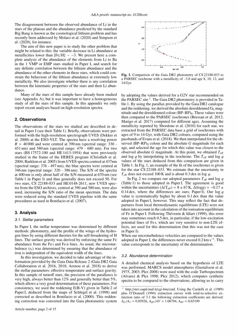
Fig. 1. Comparison of the Gaia DR2 photometry of CS 22188-033 toa PARSEC isochrone with a metallicity of –3.0 and age 8, 10, 12, and14 Gyr.

by adopting the values derived for a G2V star recommended onthe PARSEC site 1. The Gaia DR2 photometry is provided in Ta-ble 1. By using the parallax provided by the Gaia DR2 catalogueand the reddening, we derived the absolute dereddenned G0 mag-nitude and the dereddenned colour (BP–RP)0. These values werethen compared to the PARSEC isochrones (Bressan et al. 2012;Marigo et al. 2017) computed for different ages. Assuming themetallicity reported by Sbordone et al. (2010) for each star, weextracted from the PARSEC data base a grid of isochrones withages of 9 to 14 Gyr, with Gaia DR2 colours, computed using thepassbands of Evans et al. (2018). We then interpolated for the ob-served (BP–RP)0 colour and the absolute G magnitude for eachage, and selected the age for which this value was closest to theobserved absolute G magnitude. At this point, we obtained Teff

and log g by interpolating in the isochrone. The Teff and log gvalues of the stars deduced from this comparison are given inTable 1. In Fig. 1, an example of the fit of the isochrones is givenfor the star CS 22188–033. We estimate that the uncertainty inTeff does not exceed 100 K and is about 0.3 dex in log g.

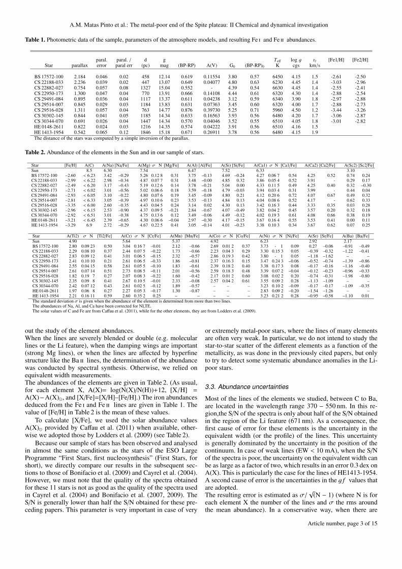
In Fig. 2 we compare our adopted parameters Teff and log g(Table 1) to those adopted in Paper I. The agreement is goodwithin the uncertainties (∆(Teff) = 8 ± 67 K, ∆(logg) = −0.17 ±0.14 dex, where the differences are ours; Paper I). Our log gvalue is systematically higher by about 0.1 dex than the valueadopted in Paper I, however. This may reflect the fact that de-partures from local thermodynamic equilibrium (LTE) were nottaken into account in the calculation of the ionisation equilibriumof Fe in Paper I. Following Thévenin & Idiart (1999), this errormay sometimes reach 0.5 dex, in particular, if the low-excitationpotential lines of Fe i, which are very sensitive to non-LTE ef-fects, are used for this determination (but this was not the casein Paper I).When our microturbulence velocities are compared to the valuesadopted in Paper I, the differences never exceed 0.2 km s−1. Thisvalue corresponds to the uncertainty of the determination.

3.2. Abundance determination

A detailed chemical analysis based on the hypothesis of LTEwas performed. MARCS model atmospheres (Gustafsson et al.1975, 2003; Plez 2008) were used with the code Turbospectrum(Alvarez & Plez 1998; Plez 2012), which computes syntheticspectra to be compared to the observations, allowing us to carry

1 http://stev.oapd.inaf.it/cgi-bin/cmd. Using the Cardelli et al. (1989)plus O’Donnell (1994) extinction curves with total-to-selective ex-tinction ratio of 3.1 the following extinction coefficients are derived:AG/AV = 0.85926, ABP/AV = 1.06794, ARP = 0.65199


http://stev.oapd.inaf.it/cgi-bin/cmd

A.M. Matas Pinto et al.: The metal-poor end of the Spite plateau: II Chemical and dynamical investigation

Table 1. Photometric data of the sample, parameters of the atmosphere models, and resulting Fe i and Fe ii abundances.

paral. paral. / d g Teff log g vt [Fe1/H] [Fe2/H]Star parallax error paral err (pc) mag (BP-RP) A(V) G0 (BP-RP)0 K cgs km/s

BS 17572-100 2.184 0.046 0.02 458 12.14 0.619 0.11554 3.80 0.57 6450 4.15 1.5 -2.61 -2.50CS 22188-033 2.236 0.039 0.02 447 13.07 0.649 0.04077 4.80 0.63 6230 4.45 1.4 -3.03 -2.96CS 22882-027 0.754 0.057 0.08 1327 15.04 0.552 - 4.39 0.54 6630 4.45 1.4 -2.55 -2.41CS 22950-173 1.300 0.047 0.04 770 13.91 0.666 0.14108 4.44 0.61 6320 4.30 1.4 -2.88 -2.54CS 29491-084 0.895 0.036 0.04 1117 13.37 0.611 0.04238 3.12 0.59 6340 3.90 1.8 -2.97 -2.88CS 29514-007 0.845 0.029 0.03 1184 13.83 0.631 0.07363 3.45 0.60 6320 4.00 1.7 -2.88 -2.73CS 29516-028 1.311 0.057 0.04 763 14.77 0.876 0.39730 5.25 0.71 5960 4.50 1.2 -3.44 -3.26CS 30302-145 0.844 0.041 0.05 1185 14.34 0.633 0.16563 3.93 0.56 6480 4.20 1.7 -3.06 -2.87CS 30344-070 0.691 0.026 0.04 1447 14.34 0.570 0.04046 3.52 0.55 6510 4.05 1.8 -3.01 -2.82HE 0148-2611 0.822 0.024 0.03 1216 14.35 0.574 0.04222 3.91 0.56 6510 4.16 1.5HE 1413-1954 0.542 0.065 0.12 1846 15.18 0.671 0.26911 3.78 0.56 6480 4.15 1.9The distance of the stars was computed by a simple inversion of the parallax.

Table 2. Abundance of the elements in the Sun and in our sample of stars.

Star [Fe/H] A(C) A(Na) [Na/Fe] A(Mg) σ N [Mg/Fe] A(Al) [Al/Fe] A(Si) [Si/Fe] A(Ca1) σ N [Ca1/Fe] A(Ca2) [Ca2/Fe] A(Sc2) [Sc2/Fe]Sun 8.5 6.30 7.54 6.47 7.52 6.33 3.10BS 17572-100 –2.60 < 6.23 3.42 –0.29 5.26 0.12 8 0.31 3.75 –0.13 4.69 –0.24 4.27 0.06 7 0.54 4.25 0.52 0.74 0.24CS 22188-033 –2.99 < 6.22 2.98 –0.34 4.87 0.07 7 0.31 3.48 –0.00 4.85 0.32 3.86 0.05 4 0.52 3.91 - 0.29 0.17CS 22882-027 –2.49 < 6.20 3.17 –0.43 5.19 0.12 6 0.14 3.78 –0.21 5.04 0.00 4.33 0.11 5 0.49 4.25 0.40 0.32 –0.30CS 22950-173 –2.71 < 6.02 3.01 –0.56 5.02 0.06 6 0.18 3.59 –0.18 4.79 –0.03 3.94 0.03 4 0.31 3.99 - 0.44 0.04CS 29491-084 –2.93 < 6.05 3.10 –0.22 4.80 0.07 6 0.19 3.45 –0.09 4.80 0.21 4.12 0.20 6 0.72 4.07 0.67 0.49 0.32CS 29514-007 –2.81 < 6.33 3.05 –0.39 4.97 0.10 6 0.23 3.53 –0.13 4.84 0.13 4.04 0.08 6 0.52 4.17 - 0.62 0.33CS 29516-028 –3.35 < 6.00 2.60 –0.35 4.43 0.04 5 0.24 3.14 0.02 4.30 0.13 3.42 0.16 3 0.44 3.33 0.35 0.03 0.28CS 30302-145 –2.96 < 6.15 2.53 –0.90 4.37 0.09 5 –0.21 2.84 –0.67 4.07 –0.49 3.82 0.04 2 0.45 3.57 0.20 0.32 0.18CS 30344-070 –2.92 < 6.51 3.01 –0.38 4.75 0.13 6 0.12 3.49 –0.06 4.49 –0.12 4.02 0.19 3 0.61 4.08 0.66 0.38 0.19HE 0148-2611 –3.21 < 6.45 2.39 –0.65 4.30 0.06 6 –0.04 2.97 –0.30 4.17 –0.15 3.67 0.16 4 0.55 3.53 0.41 0.00 0.11HE 1413-1954 –3.29 6.9 2.72 –0.29 4.67 0.22 5 0.41 3.05 –0.14 4.01 –0.23 3.38 0.10 3 0.34 3.67 0.62 0.07 0.25

Star A(Ti2) σ N [Ti2/Fe] A(Cr) σ N [Cr/Fe] A(Mn) [Mn/Fe] A(Co) σ N [Co/Fe] A(Ni) σ N [Ni/Fe] A(Sr) [Sr/Fe] A(Ba) [Ba/Fe]Sun 4.90 5.64 5.37 4.92 6.23 2.92 2.17BS 17572-100 2.80 0.09 23 0.50 3.04 0.16 7 –0.01 2.12 –0.66 2.69 0.01 2 0.37 3.73 - 1 0.09 0.27 –0.06 –0.91 –0.49CS 22188-033 2.29 0.08 10 0.37 2.44 0.07 5 –0.22 1.73 –0.66 2.23 0.04 3 0.29 3.30 0.15 3 0.05 –0.39 –0.32 –1.22 –0.41CS 22882-027 2.83 0.09 12 0.41 3.01 0.06 5 –0.15 2.32 –0.57 2.86 0.19 3 0.42 3.80 - 1 0.05 –1.18 –1.62 – –CS 22950-173 2.41 0.10 10 0.21 2.61 0.06 5 –0.33 1.86 –0.81 2.37 0.16 3 0.15 3.47 0.24 3 –0.06 –0.52 –0.74 –1.39 –0.86CS 29491-084 2.55 0.04 15 0.58 2.61 0.05 5 –0.10 1.83 –0.61 2.39 0.18 2 0.40 3.38 0.17 3 0.08 –0.17 –0.16 –1.16 –0.40CS 29514-007 2.61 0.07 14 0.51 2.73 0.08 5 –0.11 2.01 –0.56 2.59 0.18 3 0.48 3.39 0.07 2 –0.04 –0.12 –0.23 –0.96 –0.33CS 29516-028 1.82 0.19 7 0.27 2.07 0.08 3 –0.22 1.60 –0.42 2.17 0.01 2 0.60 3.08 0.02 2 0.20 –0.74 –0.31 –1.98 –0.80CS 30302-145 2.35 0.09 8 0.41 2.67 0.10 5 –0.01 2.33 –0.08 2.57 0.04 2 0.61 3.55 0.09 2 0.28 –1.13 –1.09 – –CS 30344-070 2.42 0.07 12 0.43 2.61 0.02 5 –0.12 1.89 –0.57 – – – 3.23 0.10 2 –0.09 –0.17 –0.17 –1.09 –0.35HE 0148-2611 1.97 0.06 8 0.27 2.27 0.05 3 –0.17 1.30 –0.87 – – – 2.83 0.09 2 –0.20 –1.54 –1.26 – –HE 1413-1954 2.21 0.16 11 0.59 2.60 0.35 2 0.25 – – – – – 3.23 0.21 2 0.28 –0.95 –0.58 –1.10 0.01The standard deviation σ is given when the abundance of the element is determined from more than two lines.The abundances of Na, Al, and Ca have been corrected for NLTE.The solar values of C and Fe are from Caffau et al. (2011), while for the other elements, they are from Lodders et al. (2009).

out the study of the element abundances.When the lines are severely blended or double (e.g. molecularlines or the Li feature), when the damping wings are important(strong Mg lines), or when the lines are affected by hyperfinestructure like the Ba ii lines, the determination of the abundancewas conducted by spectral synthesis. Otherwise, we relied onequivalent width measurements.The abundances of the elements are given in Table 2. (As usual,for each element X, A(X)= log(N(X)/N(H))+12, [X/H] =A(X)−A(X)�, and [X/Fe]=[X/H]–[Fe/H].) The iron abundancesdeduced from the Fe i and Fe ii lines are given in Table 1. Thevalue of [Fe/H] in Table 2 is the mean of these values.

To calculate [X/Fe], we used the solar abundance valuesA(X)� provided by Caffau et al. (2011) when available, other-wise we adopted those by Lodders et al. (2009) (see Table 2).

Because our sample of stars has been observed and analysedin almost the same conditions as the stars of the ESO LargeProgramme “First Stars, first nucleosynthesis” (First Stars, forshort), we directly compare our results in the subsequent sec-tions to those of Bonifacio et al. (2009) and Cayrel et al. (2004).However, we must note that the quality of the spectra obtainedfor these 11 stars is not as good as the quality of the spectra usedin Cayrel et al. (2004) and Bonifacio et al. (2007, 2009). TheS/N is generally lower than half the S/N obtained for these pre-ceding papers. This parameter is very important in case of very

or extremely metal-poor stars, where the lines of many elementsare often very weak. In particular, we do not intend to study thestar-to-star scatter of the different elements as a function of themetallicity, as was done in the previously cited papers, but onlyto try to detect some systematic abundance anomalies in the Li-poor stars.

3.3. Abundance uncertainties

Most of the lines of the elements we studied, between C to Ba,are located in the wavelength range 370 – 550 nm. In this re-gion,the S/N of the spectra is only about half of the S/N obtainedin the region of the Li feature (671 nm). As a consequence, thefirst cause of error for these elements is the uncertainty in theequivalent width (or the profile) of the lines. This uncertaintyis generally dominated by the uncertainty in the position of thecontinuum. In case of weak lines (EW < 10 mA), when the S/Nof the spectra is poor, the uncertainty on the equivalent width canbe as large as a factor of two, which results in an error 0.3 dex onA(X). This is particularly the case for the lines of HE1413-1954.A second cause of error is the uncertainties in the g f values thatare adopted.The resulting error is estimated as σ/

√(N − 1) (where N is for

each element X the number of the lines and σ the rms aroundthe mean abundance). In a conservative way, when there are



Fig. 2. Comparison of the Teff and log g we adopted and the values ofthe 3D model adopted in Paper I.

only two lines, an error of 0.15 dex was adopted even if it wasσ < 0.15 dex. In case of only one line, we adopted an error of0.2 dex.

To determine the uncertainties in the abundance determina-tions A(X) or [X/H], the uncertainties in Teff , log g, and micro-turbulence vt must be also considered. For these turnoff metal-poor stars, the adopted uncertainties on Teff , log g, and vt are100 K, 0.3 dex, and 0.2 km s−1(see Sec 3.1). Following Bonifacioet al. (2009), these values correspond to an uncertainty on [Fe/H]of about 0.11 dex. We also computed the error on A(Li) due tothe uncertainty in the atmospheric parameters (not given in Boni-facio et al. 2009). For turnoff stars, this error is about 0.07 dex,and it is dominated by the error on the effective temperature. Thetotal error on A(X) or [X/H] includes errors linked to the choiceof stellar parameters of the model and to observations.

For elements X heavier than Li, the interesting value is theratio [X/Fe]. For most of the elements, an error on, for example,the temperature of the model induces about the same error onA(Fe) and A(X), and as a consequence, the error on [X/Fe] issmall. We have adopted the values given in the Table 4 of Boni-facio et al. (2009), taking into account (linearly) that in our casethe adopted error on log g is three times larger.

3.4. Lithium

3.4.1. 1D LTE computation

The lithium analysis was first conducted by spectral synthesis,investigating the Li 670.7 nm resonance doublet. The adoptedatomic data for the Li doublet are the same as those used byBonifacio et al. (2007) and Sbordone et al. (2010); they are basedon Asplund et al. (2006). They take into account the hyperfinestructure of the lines and also the isotopic components for an as-sumed solar isotopic ratio. The abundance A(Li), based on one-

Table 3. Lithium abundances.

Star EW(Li) A(Li) A(Li)S/N [pm] 1D LTE error 3D NLTE

BS 17572-100 190 1.71 2.19 0.08 2.16CS 22188-033* 220 0.90 1.74 0.08 1.72CS 22882-027 80 < 0.56 < 1.60 0.10 < 1.56CS 22950-173 90 2.25 2.23 0.10 2.20CS 29491-084 100 1.86 2.15 0.10 2.13CS 29514-007 90 2.49 2.27 0.10 2.25CS 29516-028 60 2.46 2.01 0.13 2.02CS 30302-145 70 1.59 2.17 0.12 2.14CS 30344-070 80 1.70 2.22 0.12 2.19HE 0148-2611* 200 1.26 2.08 0.08 2.05HE 1413-1954 50 1.62 2.17 0.13 2.14An asterisk means that new spectra have been obtained.

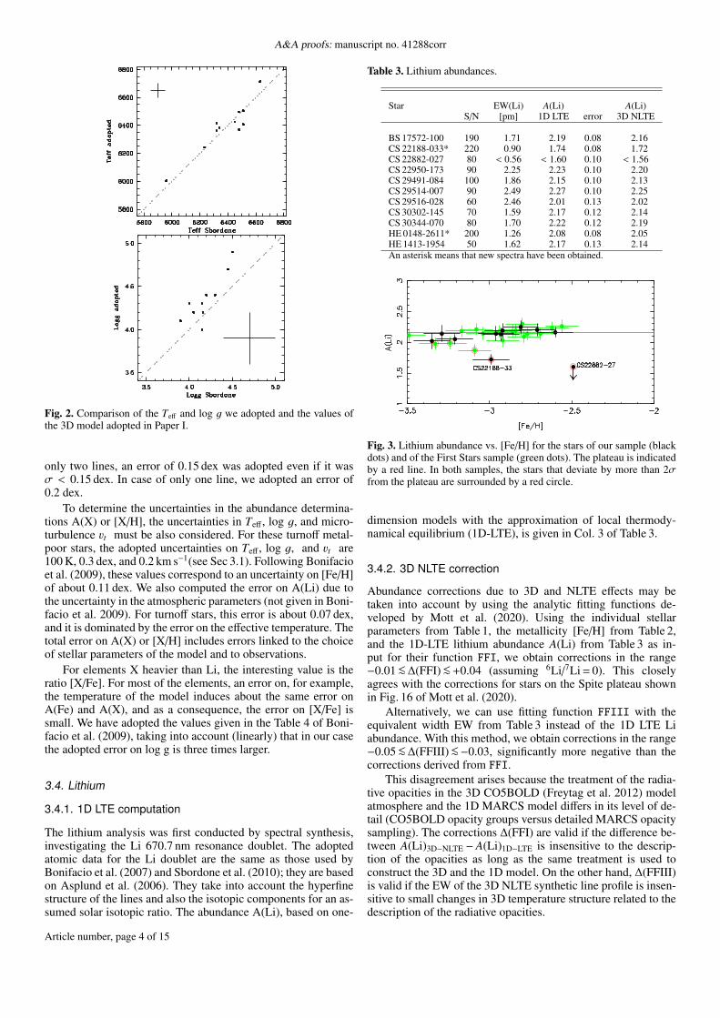
Fig. 3. Lithium abundance vs. [Fe/H] for the stars of our sample (blackdots) and of the First Stars sample (green dots). The plateau is indicatedby a red line. In both samples, the stars that deviate by more than 2σfrom the plateau are surrounded by a red circle.

dimension models with the approximation of local thermody-namical equilibrium (1D-LTE), is given in Col. 3 of Table 3.

3.4.2. 3D NLTE correction

Abundance corrections due to 3D and NLTE effects may betaken into account by using the analytic fitting functions de-veloped by Mott et al. (2020). Using the individual stellarparameters from Table 1, the metallicity [Fe/H] from Table 2,and the 1D-LTE lithium abundance A(Li) from Table 3 as in-put for their function FFI, we obtain corrections in the range−0.01<∼∆(FFI)<∼+0.04 (assuming 6Li/7Li = 0). This closelyagrees with the corrections for stars on the Spite plateau shownin Fig. 16 of Mott et al. (2020).

Alternatively, we can use fitting function FFIII with theequivalent width EW from Table 3 instead of the 1D LTE Liabundance. With this method, we obtain corrections in the range−0.05<∼∆(FFIII)<∼−0.03, significantly more negative than thecorrections derived from FFI.

This disagreement arises because the treatment of the radia-tive opacities in the 3D CO5BOLD (Freytag et al. 2012) modelatmosphere and the 1D MARCS model differs in its level of de-tail (CO5BOLD opacity groups versus detailed MARCS opacitysampling). The corrections ∆(FFI) are valid if the difference be-tween A(Li)3D−NLTE − A(Li)1D−LTE is insensitive to the descrip-tion of the opacities as long as the same treatment is used toconstruct the 3D and the 1D model. On the other hand, ∆(FFIII)is valid if the EW of the 3D NLTE synthetic line profile is insen-sitive to small changes in 3D temperature structure related to thedescription of the radiative opacities.



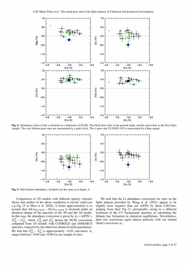
Fig. 4. Abundance ratios of the α-elements as a functions of [Fe/H]. The black dots refer to the present study, and the green dots to the First Starssample. The very lithium-poor stars are surrounded by a pink circle. The α-poor star CS 30302-145 is represented by a blue square.

Fig. 5. Odd element abundance. Symbols are the same as in figure. 4.

Comparison of 1D models with different opacity schemesshows that neither of the above conditions is strictly valid (seee.g. Fig. 15 in Mott et al. 2020). A better approximation is toassume that A(Li)3D−NLTE − A(Li)1D−NLTE is invariant under anidentical change of the opacities in the 3D and the 1D model.In this case, the abundance correction is given by ∆3 = ∆(FFI) +

∆(0)1D − ∆

(1)1D , where ∆

(0)1D and ∆

(1)1D denote the NLTE corrections

computed from 1D models with CO5BOLD and OSMARCSopacities, respectively, but otherwise identical stellar parameters.We find that ∆

(0)1D − ∆

(1)1D is approximately −0.03, and hence ∆3

ranges between −0.04 and +0.00 for our sample of stars.

We note that the Li abundance corrections for stars on theSpite plateau provided by Wang et al. (2021) appear to beslightly more negative than our ∆(FFI) by about 0.003 dex,judging from their Fig. 11, presumably owing to a differenttreatment of the UV background opacities in calculating thelithium line formation in statistical equilibrium. Nevertheless,their raw corrections agree almost perfectly with our refined(final) corrections ∆3.



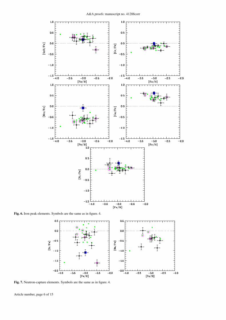
Fig. 6. Iron peak elements. Symbols are the same as in figure. 4.

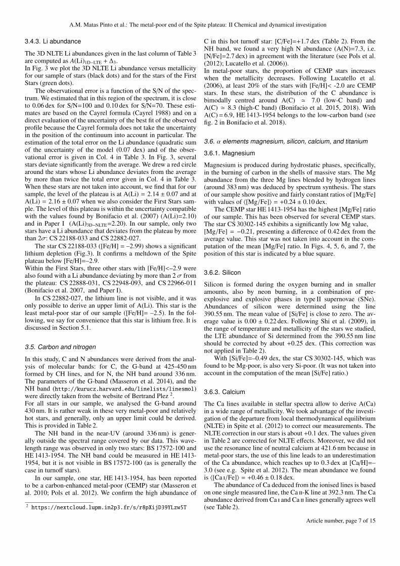
Fig. 7. Neutron-capture elements. Symbols are the same as in figure. 4.



3.4.3. Li abundance

The 3D NLTE Li abundances given in the last column of Table 3are computed as A(Li)1D−LTE + ∆3.In Fig. 3 we plot the 3D NLTE Li abundance versus metallicityfor our sample of stars (black dots) and for the stars of the FirstStars (green dots).

The observational error is a function of the S/N of the spec-trum. We estimated that in this region of the spectrum, it is closeto 0.06 dex for S/N=100 and 0.10 dex for S/N=70. These esti-mates are based on the Cayrel formula (Cayrel 1988) and on adirect evaluation of the uncertainty of the best fit of the observedprofile because the Cayrel formula does not take the uncertaintyin the position of the continuum into account in particular. Theestimation of the total error on the Li abundance (quadratic sumof the uncertainty of the model (0.07 dex) and of the obser-vational error is given in Col. 4 in Table 3. In Fig. 3, severalstars deviate significantly from the average. We drew a red circlearound the stars whose Li abundance deviates from the averageby more than twice the total error given in Col. 4 in Table 3.When these stars are not taken into account, we find that for oursample, the level of the plateau is at A(Li) = 2.14 ± 0.07 and atA(Li) = 2.16 ± 0.07 when we also consider the First Stars sam-ple. The level of this plateau is within the uncertainty compatiblewith the values found by Bonifacio et al. (2007) (A(Li)=2.10)and in Paper I (A(Li)3D−NLTE=2.20). In our sample, only twostars have a Li abundance that deviates from the plateau by morethan 2σ: CS 22188-033 and CS 22882-027.

The star CS 22188-033 ([Fe/H] = –2.99) shows a significantlithium depletion (Fig.3). It confirms a meltdown of the Spiteplateau below [Fe/H]=–2.9.Within the First Stars, three other stars with [Fe/H]<–2.9 werealso found with a Li abundance deviating by more than 2 σ fromthe plateau: CS 22888-031, CS 22948-093, and CS 22966-011(Bonifacio et al. 2007, and Paper I).

In CS 22882-027, the lithium line is not visible, and it wasonly possible to derive an upper limit of A(Li). This star is theleast metal-poor star of our sample ([Fe/H]= –2.5). In the fol-lowing, we say for convenience that this star is lithium free. It isdiscussed in Section 5.1.

3.5. Carbon and nitrogen

In this study, C and N abundances were derived from the anal-ysis of molecular bands: for C, the G-band at 425-450 nmformed by CH lines, and for N, the NH band around 336 nm.The parameters of the G-band (Masseron et al. 2014), and theNH band (http://kurucz.harvard.edu/linelists/linesmol)were directly taken from the website of Bertrand Plez 2.For all stars in our sample, we analysed the G-band around430 nm. It is rather weak in these very metal-poor and relativelyhot stars, and generally, only an upper limit could be derived.This is provided in Table 2.

The NH band in the near-UV (around 336 nm) is gener-ally outside the spectral range covered by our data. This wave-length range was observed in only two stars: BS 17572-100 andHE 1413-1954. The NH band could be measured in HE 1413-1954, but it is not visible in BS 17572-100 (as is generally thecase in turnoff stars).

In our sample, one star, HE 1413-1954, has been reportedto be a carbon-enhanced metal-poor (CEMP) star (Masseron etal. 2010; Pols et al. 2012). We confirm the high abundance of

2 https://nextcloud.lupm.in2p3.fr/s/r8pXijD39YLzw5T

C in this hot turnoff star: [C/Fe]=+1.7 dex (Table 2). From theNH band, we found a very high N abundance (A(N)=7.3, i.e.[N/Fe]=2.7 dex) in agreement with the literature (see Pols et al.(2012); Lucatello et al. (2006)).In metal-poor stars, the proportion of CEMP stars increaseswhen the metallicity decreases. Following Lucatello et al.(2006), at least 20% of the stars with [Fe/H]< -2.0 are CEMPstars. In these stars, the distribution of the C abundance isbimodally centred around A(C) ' 7.0 (low-C band) andA(C) ' 8.3 (high-C band) (Bonifacio et al. 2015, 2018). WithA(C) = 6.9, HE 1413-1954 belongs to the low-carbon band (seefig. 2 in Bonifacio et al. 2018).

3.6. α elements magnesium, silicon, calcium, and titanium

3.6.1. Magnesium

Magnesium is produced during hydrostatic phases, specifically,in the burning of carbon in the shells of massive stars. The Mgabundance from the three Mg lines blended by hydrogen lines(around 383 nm) was deduced by spectrum synthesis. The starsof our sample show positive and fairly constant ratios of [Mg/Fe]with values of 〈[Mg/Fe]〉 = +0.24 ± 0.10 dex.

The CEMP star HE 1413-1954 has the highest [Mg/Fe] ratioof our sample. This has been observed for several CEMP stars.The star CS 30302-145 exhibits a significantly low Mg value,[Mg/Fe] = −0.21, presenting a difference of 0.42 dex from theaverage value. This star was not taken into account in the com-putation of the mean [Mg/Fe] ratio. In Figs. 4, 5, 6, and 7, theposition of this star is indicated by a blue square.

3.6.2. Silicon

Silicon is formed during the oxygen burning and in smalleramounts, also by neon burning, in a combination of pre-explosive and explosive phases in type II supernovae (SNe).Abundances of silicon were determined using the line390.55 nm. The mean value of [Si/Fe] is close to zero. The av-erage value is 0.00 ± 0.22 dex. Following Shi et al. (2009), inthe range of temperature and metallicity of the stars we studied,the LTE abundance of Si determined from the 390.55 nm lineshould be corrected by about +0.25 dex. (This correction wasnot applied in Table 2).

With [Si/Fe]=–0.49 dex, the star CS 30302-145, which wasfound to be Mg-poor, is also very Si-poor. (It was not taken intoaccount in the computation of the mean [Si/Fe] ratio.)

3.6.3. Calcium

The Ca lines available in stellar spectra allow to derive A(Ca)in a wide range of metallicity. We took advantage of the investi-gation of the departure from local thermodynamical equilibrium(NLTE) in Spite et al. (2012) to correct our measurements. TheNLTE correction in our stars is about +0.1 dex. The values givenin Table 2 are corrected for NLTE effects. Moreover, we did notuse the resonance line of neutral calcium at 421.6 nm because inmetal-poor stars, the use of this line leads to an underestimationof the Ca abundance, which reaches up to 0.3 dex at [Ca/H]=–3.0 (see e.g. Spite et al. 2012). The mean abundance we foundis 〈[Ca i/Fe]〉 = +0.46 ± 0.18 dex.

The abundance of Ca deduced from the ionised lines is basedon one single measured line, the Ca ii-K line at 392.3 nm. The Caabundance derived from Ca i and Ca ii lines generally agrees well(see Table 2).


http://kurucz.harvard.edu/linelists/linesmol

https://nextcloud.lupm.in2p3.fr/s/r8pXijD39YLzw5T


However, we note that CS 30302-145 is an exception, and ifwe had used the abundance of Ca deduced from the Ca ii line, thisstar, poor in Mg and Si, would have the lowest value of [Ca/Fe]of our sample ([Ca/Fe]= 0.2 dex).

3.6.4. Titanium

The theoretical studies of core-collapse SNe and hypernovaepredict the ejection of large quantities of titanium (Limongi &Chieffi 2003a,b). The explosion mechanisms have a substan-tial impact on the production of titanium. The abundance of ti-tanium was derived using the lines of ionised titanium, whichis the dominant species in our sample of stars. The titanium-to-iron ratio is very consistent in all the stars of the sample:〈[Ti/Fe]〉 = 0.38 ± 0.17 dex.

3.7. Light odd-Z metals: sodium, aluminium

3.7.1. Sodium

In massive stars, sodium is created mostly during hydrostaticcarbon burning and partly during hydrogen burning through theNeNa cycle (see e.g. Cristallo et al. 2009; Romano et al. 2010).Here we studied the sodium D doublet lines (588.99 nm and589.59 nm), which are the only sodium lines observed in EMPstars. These lines are affected by NLTE effects. In Table 2 weapplied the NLTE corrections provided by Andrievsky et al.(2007). In these warm metal-poor turnoff stars, the correctionis only about −0.07 dex. The mean value of [Na/Fe] in our sam-ple is 〈[Na/Fe]〉 = −0.43 ± 0.22 dex.The Mg-Si-poor star CS 30302-145 has the lowest sodium abun-dance ratio [Na/Fe]=–0.90.

3.7.2. Aluminium

In massive stars, aluminium is a product of carbon and neonburning (Limongi & Chieffi 2003a,b; Nomoto et al. 2013). Weanalysed the resonance doublet of Al i at 394.40 and 396.15 nm.Both lines are sensitive to departure from LTE. We applied thecorrections by Andrievsky et al. (2008). In these metal-poorturnoff stars, the NLTE correction is positive and very signif-icant. It increases the LTE Al abundance by about +0.65 dex.The values given in Table 2 are corrected for NLTE. The mean[Al/Fe] value is –0.12±0.10 dex (if we do not take into accountCS 30302–145).

The [Al/Fe] value of the Mg-Si-poor star CS 30302–145 is0.55 dex lower than the average value (see Fig. 5).

3.8. Elements formed during complete and incomplete Siburning

We included the iron peak elements Sc, Cr, Mn, Fe, Co, and Ni.Iron is the most tightly bound nucleus, and the iron peak ele-ments are the last for which fusion reactions are the main modeof production. In the matter that formed the old very metal-poorstars, these elements were ejected by type II SNe, and their pro-duction occurs during Si burning in the pre-SN phase and in theexplosive phase (Limongi & Chieffi 2003a,b).

3.8.1. Scandium

Scandium is exclusively observed in its singly ionised state.Our scandium abundances were measured using the Sc ii line

at 424.68 nm. When comparing our results with the First Starssample (Bonifacio et al. 2009), we have an excellent agreement.

The nucleosynthesis of this element is linked to the mass ofthe parent stars (Chieffi & Limongi 2002). If the gas out of whichthese stars were formed had been enriched by a few SNe withslightly different masses, we could expect a high dispersion inscandium abundances, which in our case (Fig. 5) is not observed.

There is one exception: the very lithium-poor star CS 22882–027. This star stands out with the lowest scandium abundance atabout 3 σ from the mean.

The chemical evolution models of the Galaxy do not rep-resent the evolution of the abundance of this element well(Kobayashi et al. 2006; Matteucci 2016). They generally under-estimate the scandium abundance at low metallicity.

3.8.2. Chromium

The explosive combustion of silicon is the main source ofchromium (see e.g. Woosley & Weaver 1995; Chieffi & Limongi2002; Umeda & Nomoto 2002). Our LTE analysis based on Cr ilines shows the well-known decrease in [Cr/Fe] with decreasingmetallicity. Following Bergemann & Cescutti (2010), this is aneffect of NLTE on neutral chromium. The NLTE correction isabout +0.4 dex at [Fe/H]=–3 and only +0.2 dex at [Fe/H]=–2.If we apply this correction to our sample of stars and to the starsstudied in Bonifacio et al. (2009), the ratio [Cr/Fe] is practicallyconstant and close to zero in our metallicity range. The valuesgiven in Table 2 are not corrected for NLTE.

3.8.3. Manganese

At low metallicity, manganese is mainly made during siliconburning in core-collapse SNe. Our determination of the abun-dance of Mn in our sample of turnoff stars is based on the res-onance Mn triplet at 403 nm, which is known to be stronglyaffected by departure from LTE (Bergemann & Gehren 2008;Bergemann et al. 2019). This NLTE correction has not been ap-plied in Table 2 or in Fig 6. The average value is 〈[Mn/Fe]〉 =−0.64. Moreover, in Fig. 6, the most metal-poor stars seem to bemore Mn poor, but this can be explained by the strong increasein NLTE correction when the metallicity decreases (see Fig. 9 inBergemann et al. (2019)), but this correction has not been com-puted below [Fe/H]=–3.

Here again the Mg-Si-poor dwarf CS 30302-145 stands outin the sample. It shows a considerably higher manganese abun-dance than the remaining sample (see Fig. 6). This latter valuehas not been taken into account in the computation of the aver-age (its value is 0.56 dex above this average).

3.8.4. Cobalt

In our very metal-poor turnoff stars, the Co abundance is de-rived from the Co i lines at 384.5, 399.5, and 412.1 nm. Theselines are known to be widened by hyperfine splitting structureand are very sensitive to departure from LTE (Bergemann 2008;Bergemann et al. 2010). In our classical LTE analysis, we ob-serve an increase in [Co/Fe] as the stellar metallicity decreases(see Fig. 6), as was noted by McWilliam et al. (1995), Cayrel etal. (2004), and Bergemann et al. (2010), for example. Accord-ing to Bergemann et al. (2010), the NLTE correction leads to aneven stronger increase in [Co/Fe] with decreasing [Fe/H]. Chem-ical evolution models of the Galaxy fail to explain this behaviour(see e.g. Romano et al. 2010; Matteucci 2016). Bergemann et



al. (2010) suggested that compared to the predicted yields, Co isoverproduced relative to Fe in short-lived massive stars.

In Fig. 6 the Mg- and Si-poor dwarf CS 30302-145 has thehighest [Co/Fe] ratio of our sample.

3.8.5. Nickel

The mean value of the nickel-to-iron ratio is about zero (Fig. 6),〈[Ni/Fe]〉 = 0.04 ± 0.15 dex, in good agreement with the data ofBonifacio et al. (2009).The two stars CS 30302-145 and HE 1413-1954 have the high-est values of the Ni abundance with respect to iron, see Fig. 6.The error on the Ni abundance of the second star is very large,however.

3.9. Neutron-capture elements Sr and Ba

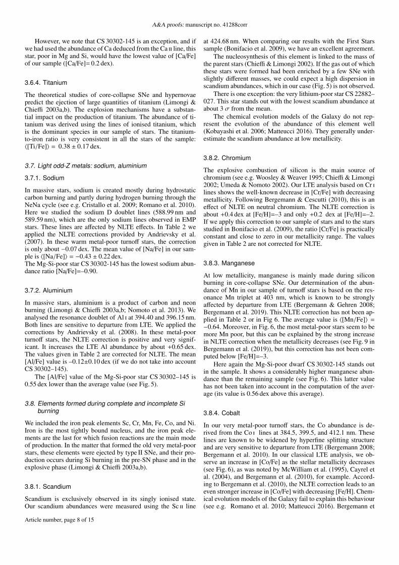
While elements up to iron are formed by nuclear fusion in anexothermic way, for heavier nuclei, fusion reactions become en-dothermic because Fe nuclei are the most tightly bound. As aconsequence, the preferred route for the formation of heaviernuclei is neutron capture (see e.g. Arnould & Goriely 2020;Cowan et al. 2021, and references therein). This capture can oc-cur through two main processes. A very rapid process (main r-process) in violent events such as explosions following the corecollapse of massive SNe, the merging of neutron stars or ofblack holes, jets, gamma ray bursts, etc. A slow process (mains-process) at a rate much lower than the β decay. This occursat the end of the evolution of relatively low-mass stars in theirasymptotic giant branch (AGB) phase. Because these low-massstars have a long lifetime, they could not enrich the matter thatformed the very old metal-poor stars we studied. In our sampleof stars, the abundance of the neutron-capture elements mainlyreflects the products of the main r-process.However, the large scatter of [Sr/Ba] for instance for a given[Ba/Fe] suggests that another mechanism is able to enrich thematter in the early Galaxy (e.g. Spite et al. 2014; Cowan et al.2021). In Fig. 8, the ratio [Sr/Ba] is plotted versus [Ba/Fe] forthe stars of the First Stars sample (dwarfs and giants) and oursample of stars. A star can be Sr rich but Ba poor. Contributionsof fast-rotating massive stars through a non-standard s-process(Meynet et al. 2006; Frischknecht et al. 2012, 2016), or super-massive AGB through an intermediate i-process (Cowan & Rose1977) are generally evoked. The contributions of these other pro-cesses become relatively high only in Ba-poor stars, where thematter that formed the star has been little enriched in heavy ele-ments by the main r−process.

In warm very metal-poor dwarf stars such as those in oursample, only the abundances of Sr and Ba are measurable in thevisible region of the spectrum. In this study, we analysed twoionised strontium lines at 407.7 nm and 421.6 nm and only theBa line at 493.4 nm because the strongest Ba line at 455.4 nmis generally outside the wavelength range of our spectra: theBa 455.4 nm line could be measured only in BS 17572-100 andHE 1413-1954.

We could measure the Ba abundance in the C-rich starHE 1413-1954, and we found (Table 2): [Ba/Fe] = 0.01 ± 0.2.This star, which belongs to the low-C band, is as expected not en-riched in Ba (see e.g. Fig. 6 in Bonifacio et al. 2015). HE 1413-1954 can be classified as a CEMP-no star (following Beers &Christlieb 2005).

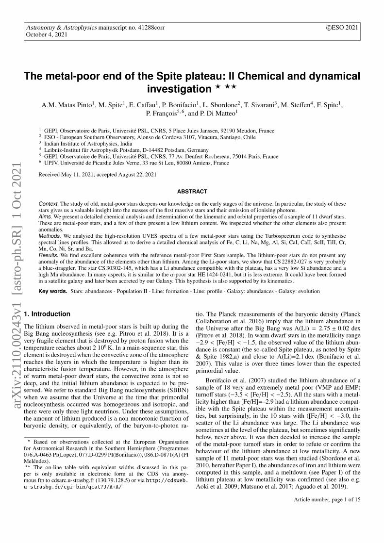
Fig. 8. [Sr/Ba] vs. [Ba/Fe]. Green symbols represent the First Stars,circles show dwarfs, and squares show giants. The black dots representour sample of dwarfs (Ba could be measured in only seven stars of thesample). The three Li-poor dwarf stars (with a measured Ba abundance)are circled in red. The dotted line represents the value [Sr/Ba] providedby the r− process alone. CS 31082-001 is a typical r-rich star, and incontrast, HD 122563, is an r-poor star with a relative enrichment of thefirst peak elements.

4. Kinematic and orbital properties of the starsample

In this section, we compare the kinematic and orbital parame-ters of our 11 stars to the First Stars sample that was extensivelystudied in Di Matteo et al. (2020). In particular, we try to detect,for instance, whether the Li-poor stars (from our sample or theFirst Stars sample) present any special characteristics.We used the GalPot code3 (Dehnen & Binney 1998) togetherwith the galactic model of McMillan (2017) to derive the kine-matical properties of our sample of stars. In this model, the dis-tance of the Sun from the Galactic centre is R� = 8.21 kpcand the local standard of rest (LSR) velocity, VLSR = 233.1km s−1(McMillan 2017). The velocity of the Sun relative to theLSR is U� = 11.1 km s−1, V� = 12.24 km s−1 and W� =7.25 km s−1(McMillan 2017). The disc rotates clockwise, and asa consequence, the z-component of the disc angular momentum,Lz, and the disc azimuthal velocity, Vphi, are negative. A starwith negative Lz and Vphi is prograde.

The positions, proper motions, and parallaxes of our sam-ple of stars are taken from Gaia DR2, but the radial velocitieswere measured on the spectra (Table 1 in Paper I) with a preci-sion of 1 km s−1. The sample of stars we studied has about thesame distance distribution, between 0.4 and 1.9 kpc (Table 1),as the sample of dwarfs studied in the frame of the First Stars(Di Matteo et al. 2020), which is used here also as a chemicalcomparison sample. The error on the parallax for all the stars islower than 12% (see Table 1). The main kinematical data andorbital properties of these stars are presented in Table 4.•X, Y, Z are the galactic coordinates of the stars, and VX , VY , VZtheir velocities in the three directions. X, Y, Z, are given in kpcand the velocities in km s−1.• R =

√X2 + Y2 is the distance of the star to the Galactic centre

in kpc, and VR is the component of the velocity in this direction:VR = (XVX + YVY )/R.• Lz, the z component of the angular momentum, is equal toXVY − YVX .3 https://github.com/PaulMcMillan-Astro/GalPot


https://github.com/PaulMcMillan-Astro/GalPot


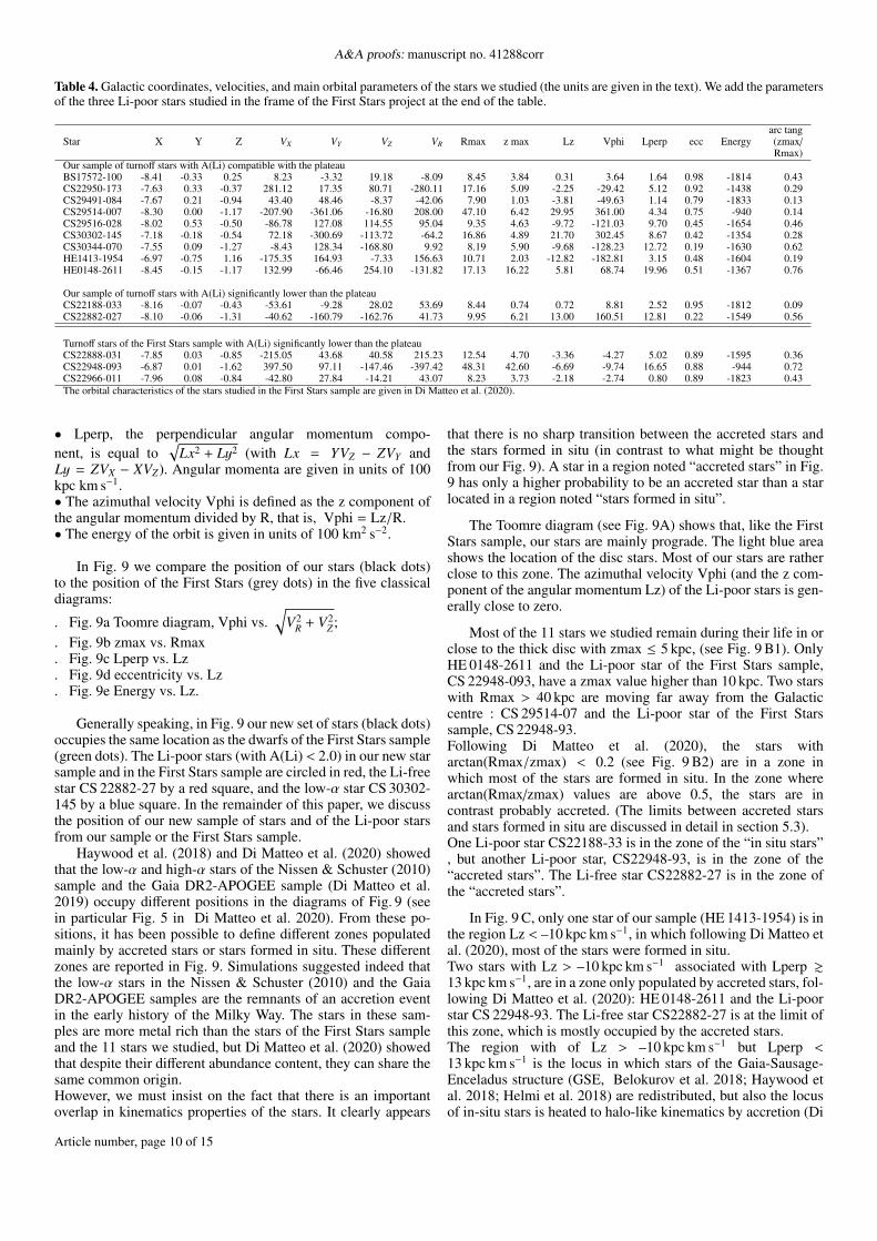
Table 4. Galactic coordinates, velocities, and main orbital parameters of the stars we studied (the units are given in the text). We add the parametersof the three Li-poor stars studied in the frame of the First Stars project at the end of the table.

arc tangStar X Y Z VX VY VZ VR Rmax z max Lz Vphi Lperp ecc Energy (zmax/

Rmax)Our sample of turnoff stars with A(Li) compatible with the plateauBS17572-100 -8.41 -0.33 0.25 8.23 -3.32 19.18 -8.09 8.45 3.84 0.31 3.64 1.64 0.98 -1814 0.43CS22950-173 -7.63 0.33 -0.37 281.12 17.35 80.71 -280.11 17.16 5.09 -2.25 -29.42 5.12 0.92 -1438 0.29CS29491-084 -7.67 0.21 -0.94 43.40 48.46 -8.37 -42.06 7.90 1.03 -3.81 -49.63 1.14 0.79 -1833 0.13CS29514-007 -8.30 0.00 -1.17 -207.90 -361.06 -16.80 208.00 47.10 6.42 29.95 361.00 4.34 0.75 -940 0.14CS29516-028 -8.02 0.53 -0.50 -86.78 127.08 114.55 95.04 9.35 4.63 -9.72 -121.03 9.70 0.45 -1654 0.46CS30302-145 -7.18 -0.18 -0.54 72.18 -300.69 -113.72 -64.2 16.86 4.89 21.70 302.45 8.67 0.42 -1354 0.28CS30344-070 -7.55 0.09 -1.27 -8.43 128.34 -168.80 9.92 8.19 5.90 -9.68 -128.23 12.72 0.19 -1630 0.62HE1413-1954 -6.97 -0.75 1.16 -175.35 164.93 -7.33 156.63 10.71 2.03 -12.82 -182.81 3.15 0.48 -1604 0.19HE0148-2611 -8.45 -0.15 -1.17 132.99 -66.46 254.10 -131.82 17.13 16.22 5.81 68.74 19.96 0.51 -1367 0.76

Our sample of turnoff stars with A(Li) significantly lower than the plateauCS22188-033 -8.16 -0.07 -0.43 -53.61 -9.28 28.02 53.69 8.44 0.74 0.72 8.81 2.52 0.95 -1812 0.09CS22882-027 -8.10 -0.06 -1.31 -40.62 -160.79 -162.76 41.73 9.95 6.21 13.00 160.51 12.81 0.22 -1549 0.56

Turnoff stars of the First Stars sample with A(Li) significantly lower than the plateauCS22888-031 -7.85 0.03 -0.85 -215.05 43.68 40.58 215.23 12.54 4.70 -3.36 -4.27 5.02 0.89 -1595 0.36CS22948-093 -6.87 0.01 -1.62 397.50 97.11 -147.46 -397.42 48.31 42.60 -6.69 -9.74 16.65 0.88 -944 0.72CS22966-011 -7.96 0.08 -0.84 -42.80 27.84 -14.21 43.07 8.23 3.73 -2.18 -2.74 0.80 0.89 -1823 0.43The orbital characteristics of the stars studied in the First Stars sample are given in Di Matteo et al. (2020).

• Lperp, the perpendicular angular momentum compo-nent, is equal to

√Lx2 + Ly2 (with Lx = YVZ − ZVY and

Ly = ZVX − XVZ). Angular momenta are given in units of 100kpc km s−1.• The azimuthal velocity Vphi is defined as the z component ofthe angular momentum divided by R, that is, Vphi = Lz/R.• The energy of the orbit is given in units of 100 km2 s−2.

In Fig. 9 we compare the position of our stars (black dots)to the position of the First Stars (grey dots) in the five classicaldiagrams:

. Fig. 9a Toomre diagram, Vphi vs.√

V2R + V2

Z ;. Fig. 9b zmax vs. Rmax. Fig. 9c Lperp vs. Lz. Fig. 9d eccentricity vs. Lz. Fig. 9e Energy vs. Lz.

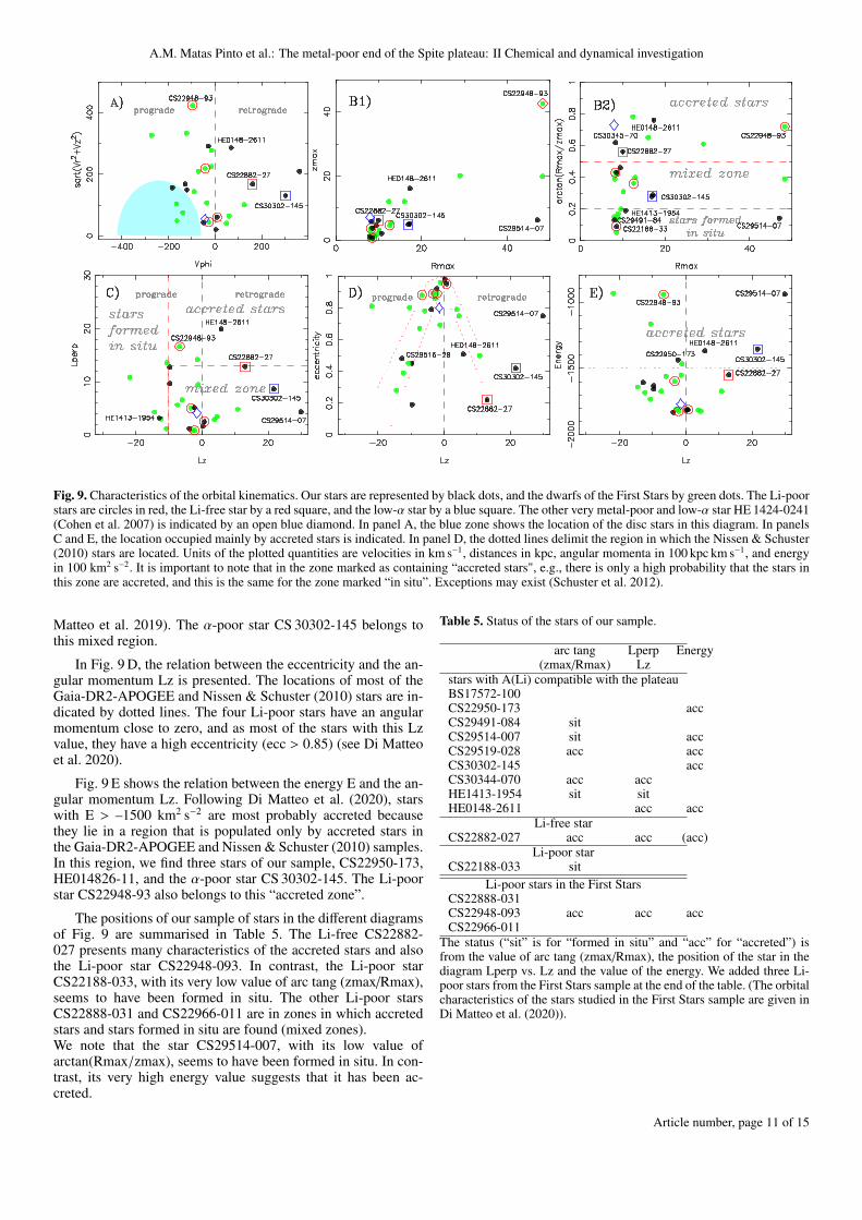
Generally speaking, in Fig. 9 our new set of stars (black dots)occupies the same location as the dwarfs of the First Stars sample(green dots). The Li-poor stars (with A(Li) < 2.0) in our new starsample and in the First Stars sample are circled in red, the Li-freestar CS 22882-27 by a red square, and the low-α star CS 30302-145 by a blue square. In the remainder of this paper, we discussthe position of our new sample of stars and of the Li-poor starsfrom our sample or the First Stars sample.

Haywood et al. (2018) and Di Matteo et al. (2020) showedthat the low-α and high-α stars of the Nissen & Schuster (2010)sample and the Gaia DR2-APOGEE sample (Di Matteo et al.2019) occupy different positions in the diagrams of Fig. 9 (seein particular Fig. 5 in Di Matteo et al. 2020). From these po-sitions, it has been possible to define different zones populatedmainly by accreted stars or stars formed in situ. These differentzones are reported in Fig. 9. Simulations suggested indeed thatthe low-α stars in the Nissen & Schuster (2010) and the GaiaDR2-APOGEE samples are the remnants of an accretion eventin the early history of the Milky Way. The stars in these sam-ples are more metal rich than the stars of the First Stars sampleand the 11 stars we studied, but Di Matteo et al. (2020) showedthat despite their different abundance content, they can share thesame common origin.However, we must insist on the fact that there is an importantoverlap in kinematics properties of the stars. It clearly appears

that there is no sharp transition between the accreted stars andthe stars formed in situ (in contrast to what might be thoughtfrom our Fig. 9). A star in a region noted “accreted stars” in Fig.9 has only a higher probability to be an accreted star than a starlocated in a region noted “stars formed in situ”.

The Toomre diagram (see Fig. 9A) shows that, like the FirstStars sample, our stars are mainly prograde. The light blue areashows the location of the disc stars. Most of our stars are ratherclose to this zone. The azimuthal velocity Vphi (and the z com-ponent of the angular momentum Lz) of the Li-poor stars is gen-erally close to zero.

Most of the 11 stars we studied remain during their life in orclose to the thick disc with zmax ≤ 5 kpc, (see Fig. 9 B1). OnlyHE 0148-2611 and the Li-poor star of the First Stars sample,CS 22948-093, have a zmax value higher than 10 kpc. Two starswith Rmax > 40 kpc are moving far away from the Galacticcentre : CS 29514-07 and the Li-poor star of the First Starssample, CS 22948-93.Following Di Matteo et al. (2020), the stars witharctan(Rmax/zmax) < 0.2 (see Fig. 9 B2) are in a zone inwhich most of the stars are formed in situ. In the zone wherearctan(Rmax/zmax) values are above 0.5, the stars are incontrast probably accreted. (The limits between accreted starsand stars formed in situ are discussed in detail in section 5.3).One Li-poor star CS22188-33 is in the zone of the “in situ stars”, but another Li-poor star, CS22948-93, is in the zone of the“accreted stars”. The Li-free star CS22882-27 is in the zone ofthe “accreted stars”.

In Fig. 9 C, only one star of our sample (HE 1413-1954) is inthe region Lz < –10 kpc km s−1, in which following Di Matteo etal. (2020), most of the stars were formed in situ.Two stars with Lz > –10 kpc km s−1 associated with Lperp &13 kpc km s−1, are in a zone only populated by accreted stars, fol-lowing Di Matteo et al. (2020): HE 0148-2611 and the Li-poorstar CS 22948-93. The Li-free star CS22882-27 is at the limit ofthis zone, which is mostly occupied by the accreted stars.The region with of Lz > –10 kpc km s−1 but Lperp <13 kpc km s−1 is the locus in which stars of the Gaia-Sausage-Enceladus structure (GSE, Belokurov et al. 2018; Haywood etal. 2018; Helmi et al. 2018) are redistributed, but also the locusof in-situ stars is heated to halo-like kinematics by accretion (Di



Fig. 9. Characteristics of the orbital kinematics. Our stars are represented by black dots, and the dwarfs of the First Stars by green dots. The Li-poorstars are circles in red, the Li-free star by a red square, and the low-α star by a blue square. The other very metal-poor and low-α star HE 1424-0241(Cohen et al. 2007) is indicated by an open blue diamond. In panel A, the blue zone shows the location of the disc stars in this diagram. In panelsC and E, the location occupied mainly by accreted stars is indicated. In panel D, the dotted lines delimit the region in which the Nissen & Schuster(2010) stars are located. Units of the plotted quantities are velocities in km s−1, distances in kpc, angular momenta in 100 kpc km s−1, and energyin 100 km2 s−2. It is important to note that in the zone marked as containing “accreted stars", e.g., there is only a high probability that the stars inthis zone are accreted, and this is the same for the zone marked “in situ”. Exceptions may exist (Schuster et al. 2012).

Matteo et al. 2019). The α-poor star CS 30302-145 belongs tothis mixed region.

In Fig. 9 D, the relation between the eccentricity and the an-gular momentum Lz is presented. The locations of most of theGaia-DR2-APOGEE and Nissen & Schuster (2010) stars are in-dicated by dotted lines. The four Li-poor stars have an angularmomentum close to zero, and as most of the stars with this Lzvalue, they have a high eccentricity (ecc > 0.85) (see Di Matteoet al. 2020).

Fig. 9 E shows the relation between the energy E and the an-gular momentum Lz. Following Di Matteo et al. (2020), starswith E > –1500 km2 s−2 are most probably accreted becausethey lie in a region that is populated only by accreted stars inthe Gaia-DR2-APOGEE and Nissen & Schuster (2010) samples.In this region, we find three stars of our sample, CS22950-173,HE014826-11, and the α-poor star CS 30302-145. The Li-poorstar CS22948-93 also belongs to this “accreted zone”.

The positions of our sample of stars in the different diagramsof Fig. 9 are summarised in Table 5. The Li-free CS22882-027 presents many characteristics of the accreted stars and alsothe Li-poor star CS22948-093. In contrast, the Li-poor starCS22188-033, with its very low value of arc tang (zmax/Rmax),seems to have been formed in situ. The other Li-poor starsCS22888-031 and CS22966-011 are in zones in which accretedstars and stars formed in situ are found (mixed zones).We note that the star CS29514-007, with its low value ofarctan(Rmax/zmax), seems to have been formed in situ. In con-trast, its very high energy value suggests that it has been ac-creted.

Table 5. Status of the stars of our sample.

arc tang Lperp Energy(zmax/Rmax) Lz

stars with A(Li) compatible with the plateauBS17572-100CS22950-173 accCS29491-084 sitCS29514-007 sit accCS29519-028 acc accCS30302-145 accCS30344-070 acc accHE1413-1954 sit sitHE0148-2611 acc acc

Li-free starCS22882-027 acc acc (acc)

Li-poor starCS22188-033 sit

Li-poor stars in the First StarsCS22888-031CS22948-093 acc acc accCS22966-011

The status (“sit” is for “formed in situ” and “acc” for “accreted”) isfrom the value of arc tang (zmax/Rmax), the position of the star in thediagram Lperp vs. Lz and the value of the energy. We added three Li-poor stars from the First Stars sample at the end of the table. (The orbitalcharacteristics of the stars studied in the First Stars sample are given inDi Matteo et al. (2020)).



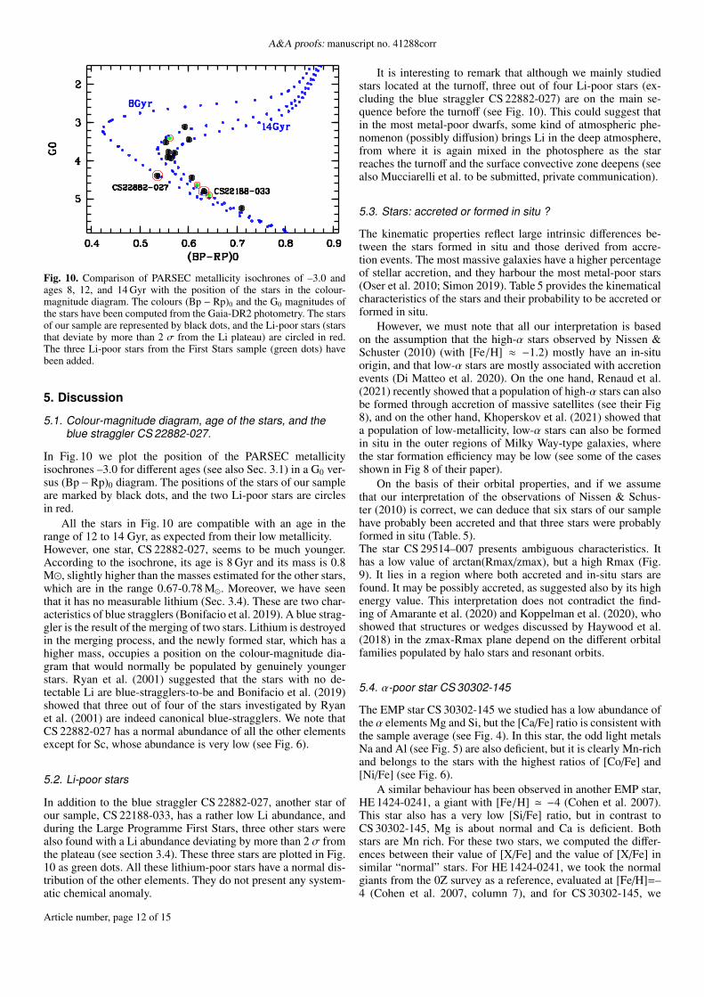
Fig. 10. Comparison of PARSEC metallicity isochrones of –3.0 andages 8, 12, and 14 Gyr with the position of the stars in the colour-magnitude diagram. The colours (Bp − Rp)0 and the G0 magnitudes ofthe stars have been computed from the Gaia-DR2 photometry. The starsof our sample are represented by black dots, and the Li-poor stars (starsthat deviate by more than 2 σ from the Li plateau) are circled in red.The three Li-poor stars from the First Stars sample (green dots) havebeen added.

5. Discussion

5.1. Colour-magnitude diagram, age of the stars, and theblue straggler CS 22882-027.

In Fig. 10 we plot the position of the PARSEC metallicityisochrones –3.0 for different ages (see also Sec. 3.1) in a G0 ver-sus (Bp−Rp)0 diagram. The positions of the stars of our sampleare marked by black dots, and the two Li-poor stars are circlesin red.

All the stars in Fig. 10 are compatible with an age in therange of 12 to 14 Gyr, as expected from their low metallicity.However, one star, CS 22882-027, seems to be much younger.According to the isochrone, its age is 8 Gyr and its mass is 0.8M�, slightly higher than the masses estimated for the other stars,which are in the range 0.67-0.78 M�. Moreover, we have seenthat it has no measurable lithium (Sec. 3.4). These are two char-acteristics of blue stragglers (Bonifacio et al. 2019). A blue strag-gler is the result of the merging of two stars. Lithium is destroyedin the merging process, and the newly formed star, which has ahigher mass, occupies a position on the colour-magnitude dia-gram that would normally be populated by genuinely youngerstars. Ryan et al. (2001) suggested that the stars with no de-tectable Li are blue-stragglers-to-be and Bonifacio et al. (2019)showed that three out of four of the stars investigated by Ryanet al. (2001) are indeed canonical blue-stragglers. We note thatCS 22882-027 has a normal abundance of all the other elementsexcept for Sc, whose abundance is very low (see Fig. 6).

5.2. Li-poor stars

In addition to the blue straggler CS 22882-027, another star ofour sample, CS 22188-033, has a rather low Li abundance, andduring the Large Programme First Stars, three other stars werealso found with a Li abundance deviating by more than 2 σ fromthe plateau (see section 3.4). These three stars are plotted in Fig.10 as green dots. All these lithium-poor stars have a normal dis-tribution of the other elements. They do not present any system-atic chemical anomaly.

It is interesting to remark that although we mainly studiedstars located at the turnoff, three out of four Li-poor stars (ex-cluding the blue straggler CS 22882-027) are on the main se-quence before the turnoff (see Fig. 10). This could suggest thatin the most metal-poor dwarfs, some kind of atmospheric phe-nomenon (possibly diffusion) brings Li in the deep atmosphere,from where it is again mixed in the photosphere as the starreaches the turnoff and the surface convective zone deepens (seealso Mucciarelli et al. to be submitted, private communication).

5.3. Stars: accreted or formed in situ ?

The kinematic properties reflect large intrinsic differences be-tween the stars formed in situ and those derived from accre-tion events. The most massive galaxies have a higher percentageof stellar accretion, and they harbour the most metal-poor stars(Oser et al. 2010; Simon 2019). Table 5 provides the kinematicalcharacteristics of the stars and their probability to be accreted orformed in situ.

However, we must note that all our interpretation is basedon the assumption that the high-α stars observed by Nissen &Schuster (2010) (with [Fe/H] ≈ −1.2) mostly have an in-situorigin, and that low-α stars are mostly associated with accretionevents (Di Matteo et al. 2020). On the one hand, Renaud et al.(2021) recently showed that a population of high-α stars can alsobe formed through accretion of massive satellites (see their Fig8), and on the other hand, Khoperskov et al. (2021) showed thata population of low-metallicity, low-α stars can also be formedin situ in the outer regions of Milky Way-type galaxies, wherethe star formation efficiency may be low (see some of the casesshown in Fig 8 of their paper).

On the basis of their orbital properties, and if we assumethat our interpretation of the observations of Nissen & Schus-ter (2010) is correct, we can deduce that six stars of our samplehave probably been accreted and that three stars were probablyformed in situ (Table. 5).The star CS 29514–007 presents ambiguous characteristics. Ithas a low value of arctan(Rmax/zmax), but a high Rmax (Fig.9). It lies in a region where both accreted and in-situ stars arefound. It may be possibly accreted, as suggested also by its highenergy value. This interpretation does not contradict the find-ing of Amarante et al. (2020) and Koppelman et al. (2020), whoshowed that structures or wedges discussed by Haywood et al.(2018) in the zmax-Rmax plane depend on the different orbitalfamilies populated by halo stars and resonant orbits.

5.4. α-poor star CS 30302-145

The EMP star CS 30302-145 we studied has a low abundance ofthe α elements Mg and Si, but the [Ca/Fe] ratio is consistent withthe sample average (see Fig. 4). In this star, the odd light metalsNa and Al (see Fig. 5) are also deficient, but it is clearly Mn-richand belongs to the stars with the highest ratios of [Co/Fe] and[Ni/Fe] (see Fig. 6).

A similar behaviour has been observed in another EMP star,HE 1424-0241, a giant with [Fe/H] ' −4 (Cohen et al. 2007).This star also has a very low [Si/Fe] ratio, but in contrast toCS 30302-145, Mg is about normal and Ca is deficient. Bothstars are Mn rich. For these two stars, we computed the differ-ences between their value of [X/Fe] and the value of [X/Fe] insimilar “normal” stars. For HE 1424-0241, we took the normalgiants from the 0Z survey as a reference, evaluated at [Fe/H]=–4 (Cohen et al. 2007, column 7), and for CS 30302-145, we



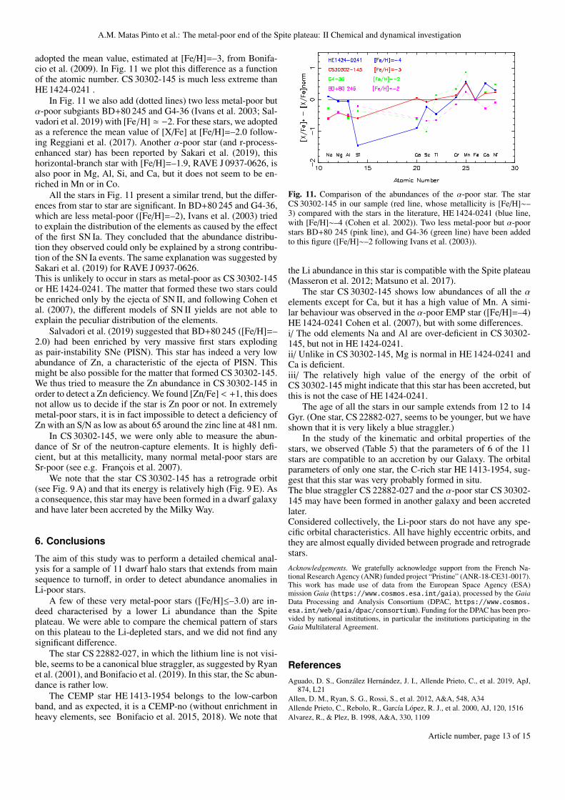
adopted the mean value, estimated at [Fe/H]=–3, from Bonifa-cio et al. (2009). In Fig. 11 we plot this difference as a functionof the atomic number. CS 30302-145 is much less extreme thanHE 1424-0241 .

In Fig. 11 we also add (dotted lines) two less metal-poor butα-poor subgiants BD+80 245 and G4-36 (Ivans et al. 2003; Sal-vadori et al. 2019) with [Fe/H] ' −2. For these stars, we adoptedas a reference the mean value of [X/Fe] at [Fe/H]=–2.0 follow-ing Reggiani et al. (2017). Another α-poor star (and r-process-enhanced star) has been reported by Sakari et al. (2019), thishorizontal-branch star with [Fe/H]=–1.9, RAVE J 0937-0626, isalso poor in Mg, Al, Si, and Ca, but it does not seem to be en-riched in Mn or in Co.

All the stars in Fig. 11 present a similar trend, but the differ-ences from star to star are significant. In BD+80 245 and G4-36,which are less metal-poor ([Fe/H]=–2), Ivans et al. (2003) triedto explain the distribution of the elements as caused by the effectof the first SN Ia. They concluded that the abundance distribu-tion they observed could only be explained by a strong contribu-tion of the SN Ia events. The same explanation was suggested bySakari et al. (2019) for RAVE J 0937-0626.This is unlikely to occur in stars as metal-poor as CS 30302-145or HE 1424-0241. The matter that formed these two stars couldbe enriched only by the ejecta of SN II, and following Cohen etal. (2007), the different models of SN II yields are not able toexplain the peculiar distribution of the elements.

Salvadori et al. (2019) suggested that BD+80 245 ([Fe/H]=–2.0) had been enriched by very massive first stars explodingas pair-instability SNe (PISN). This star has indeed a very lowabundance of Zn, a characteristic of the ejecta of PISN. Thismight be also possible for the matter that formed CS 30302-145.We thus tried to measure the Zn abundance in CS 30302-145 inorder to detect a Zn deficiency. We found [Zn/Fe] < +1, this doesnot allow us to decide if the star is Zn poor or not. In extremelymetal-poor stars, it is in fact impossible to detect a deficiency ofZn with an S/N as low as about 65 around the zinc line at 481 nm.

In CS 30302-145, we were only able to measure the abun-dance of Sr of the neutron-capture elements. It is highly defi-cient, but at this metallicity, many normal metal-poor stars areSr-poor (see e.g. François et al. 2007).

We note that the star CS 30302-145 has a retrograde orbit(see Fig. 9 A) and that its energy is relatively high (Fig. 9 E). Asa consequence, this star may have been formed in a dwarf galaxyand have later been accreted by the Milky Way.

6. Conclusions

The aim of this study was to perform a detailed chemical anal-ysis for a sample of 11 dwarf halo stars that extends from mainsequence to turnoff, in order to detect abundance anomalies inLi-poor stars.

A few of these very metal-poor stars ([Fe/H]≤–3.0) are in-deed characterised by a lower Li abundance than the Spiteplateau. We were able to compare the chemical pattern of starson this plateau to the Li-depleted stars, and we did not find anysignificant difference.

The star CS 22882-027, in which the lithium line is not visi-ble, seems to be a canonical blue straggler, as suggested by Ryanet al. (2001), and Bonifacio et al. (2019). In this star, the Sc abun-dance is rather low.

The CEMP star HE 1413-1954 belongs to the low-carbonband, and as expected, it is a CEMP-no (without enrichment inheavy elements, see Bonifacio et al. 2015, 2018). We note that

Fig. 11. Comparison of the abundances of the α-poor star. The starCS 30302-145 in our sample (red line, whose metallicity is [Fe/H]∼–3) compared with the stars in the literature, HE 1424-0241 (blue line,with [Fe/H]∼–4 (Cohen et al. 2002)). Two less metal-poor but α-poorstars BD+80 245 (pink line), and G4-36 (green line) have been addedto this figure ([Fe/H]∼–2 following Ivans et al. (2003)).

the Li abundance in this star is compatible with the Spite plateau(Masseron et al. 2012; Matsuno et al. 2017).

The star CS 30302-145 shows low abundances of all the αelements except for Ca, but it has a high value of Mn. A simi-lar behaviour was observed in the α-poor EMP star ([Fe/H]=–4)HE 1424-0241 Cohen et al. (2007), but with some differences.i/ The odd elements Na and Al are over-deficient in CS 30302-145, but not in HE 1424-0241.ii/ Unlike in CS 30302-145, Mg is normal in HE 1424-0241 andCa is deficient.iii/ The relatively high value of the energy of the orbit ofCS 30302-145 might indicate that this star has been accreted, butthis is not the case of HE 1424-0241.

The age of all the stars in our sample extends from 12 to 14Gyr. (One star, CS 22882-027, seems to be younger, but we haveshown that it is very likely a blue straggler.)

In the study of the kinematic and orbital properties of thestars, we observed (Table 5) that the parameters of 6 of the 11stars are compatible to an accretion by our Galaxy. The orbitalparameters of only one star, the C-rich star HE 1413-1954, sug-gest that this star was very probably formed in situ.The blue straggler CS 22882-027 and the α-poor star CS 30302-145 may have been formed in another galaxy and been accretedlater.Considered collectively, the Li-poor stars do not have any spe-cific orbital characteristics. All have highly eccentric orbits, andthey are almost equally divided between prograde and retrogradestars.

Acknowledgements. We gratefully acknowledge support from the French Na-tional Research Agency (ANR) funded project “Pristine” (ANR-18-CE31-0017).This work has made use of data from the European Space Agency (ESA)mission Gaia (https://www.cosmos.esa.int/gaia), processed by the GaiaData Processing and Analysis Consortium (DPAC, https://www.cosmos.esa.int/web/gaia/dpac/consortium). Funding for the DPAC has been pro-vided by national institutions, in particular the institutions participating in theGaia Multilateral Agreement.

ReferencesAguado, D. S., González Hernández, J. I., Allende Prieto, C., et al. 2019, ApJ,

874, L21Allen, D. M., Ryan, S. G., Rossi, S., et al. 2012, A&A, 548, A34Allende Prieto, C., Rebolo, R., García López, R. J., et al. 2000, AJ, 120, 1516Alvarez, R., & Plez, B. 1998, A&A, 330, 1109


https://www.cosmos.esa.int/gaia

https://www.cosmos.esa.int/web/gaia/dpac/consortium

https://www.cosmos.esa.int/web/gaia/dpac/consortium


Amarante, J. A. S., Smith, M. C., & Boeche, C. 2020, MNRAS, 492, 3816.doi:10.1093/mnras/staa077

Andrievsky, S. M., Spite, M., Korotin, S. A., et al. 2007, A&A, 464, 1081Andrievsky, S. M., Spite, M., Korotin, S. A., et al. 2008, A&A, 481, 481Aoki, W., Barklem, P. S., Beers, T. C., et al. 2009, ApJ, 698, 1803.

doi:10.1088/0004-637X/698/2/1803Aoki, W., Suda, T., Boyd, R. N., et al. 2013, ApJ, 766, L13Arnould, M. & Goriely, S. 2020, Progress in Particle and Nuclear Physics, 112,

103766Arenou, F., Luri, X., Babusiaux, C., et al. 2018, A&A, 616, A17Asplund, M., Lambert, D. L., Nissen, P. E., et al. 2006, ApJ, 644, 229.

doi:10.1086/503538Barbuy, B. 1983, A&A, 123, 1Barklem, P. S., Christlieb, N., Beers, T. C., et al. 2005, A&A, 439, 129Beers, T. C. & Christlieb, N. 2005, ARA&A, 43, 531.

doi:10.1146/annurev.astro.42.053102.134057Beers, T. C. & Christlieb, N. 2005, ARA&A, 43, 531Beers, T. C., Preston, G. W., & Shectman, S. A. 1992, AJ, 103, 1987Belokurov, V., Erkal, D., Evans, N. W., et al. 2018, MNRAS, 478, 611Bergemann, M. 2008, Physica Scripta Volume T, 133, 014013Bergemann, M. & Gehren, T. 2008, A&A, 492, 823. doi:10.1051/0004-

6361:200810098Bergemann, M. & Cescutti, G. 2010, A&A, 522, A9Bergemann, M., Pickering, J. C., & Gehren, T. 2010, MNRAS, 401, 1334Bergemann, M., Gallagher, A. J., Eitner, P., et al. 2019, A&A, 631, A80Boehm-Vitense, E. 1981, ARA&A, 19, 295.

doi:10.1146/annurev.aa.19.090181.001455Bonifacio, P., Monai, S., & Beers, T. C. 2000, AJ, 120, 2065Bonifacio, P., Molaro, P., Sivarani, T., et al. 2007, A&A, 462, 851Bonifacio, P., Spite, M., Cayrel, R., et al. 2009, A&A, 501, 519Bonifacio, P., Caffau, E., Spite, M., et al. 2015, A&A, 579, A28.

doi:10.1051/0004-6361/201425266Bonifacio, P., Caffau, E., Spite, M., et al. 2018, A&A, 612, A65Bonifacio, P., Caffau, E., Spite, M., et al. 2019, Research Notes of the American

Astronomical Society, 3, 64Bressan, A., Marigo, P., Girardi, L., et al. 2012, MNRAS, 427, 127Caffau, E., Ludwig, H.-G., Steffen, M., Freytag, B., & Bonifacio, P. 2011,

Sol. Phys., 268, 255Cardelli, J. A., Clayton, G. C., & Mathis, J. S. 1989, ApJ, 345, 245.

doi:10.1086/167900Carretta, E., Gratton, R., Cohen, J. G., et al. 2002, AJ, 124, 481Cayrel, R., Depagne, E., Spite, M., et al. 2004, A&A, 416, 1117Cayrel, R. 1988, The Impact of Very High S/N Spectroscopy on Stellar Physics,

132, 345Chieffi, A. & Limongi, M. 2002, ApJ, 577, 281Christlieb, N., Beers, T. C., Barklem, P. S., et al. 2004, A&A, 428, 1027Cohen, J. G., Christlieb, N., Beers, T. C., et al. 2002, AJ, 124, 470Cohen, J. G., McWilliam, A., Christlieb, N., et al. 2007, ApJ, 659, L161Cowan, J. J. & Rose, W. K. 1977, ApJ, 212, 149. doi:10.1086/155030Cowan, J. J., Sneden, C., Lawler, J. E., et al. 2021, Reviews of Modern Physics,

93, 015002Cristallo, S., Straniero, O., Gallino, R., et al. 2009, ApJ, 696, 797Dehnen, W., & Binney, J. 1998, MNRAS, 294, 429Dekker, H., D’Odorico, S., Kaufer, A., et al. 2000, Proc. SPIE, 534Di Matteo, P., Haywood, M., Lehnert, M. D., et al. 2019, A&A, 632, A4Di Matteo, P., Spite, M., Haywood, M., et al. 2020, A&A, 636, A115Evans, D. W., Riello, M., De Angeli, F., et al. 2018, A&A, 616, A4.

doi:10.1051/0004-6361/201832756Freytag, B., Steffen, M., Ludwig, H.-G., et al. 2012, Journal of Computational

Physics, 231, 919. doi:10.1016/j.jcp.2011.09.026Frischknecht, U., Hirschi, R., & Thielemann, F.-K. 2012, A&A, 538, L2.

doi:10.1051/0004-6361/201117794Frischknecht, U., Hirschi, R., Pignatari, M., et al. 2016, MNRAS, 456, 1803.

doi:10.1093/mnras/stv2723François, P., Depagne, E., Hill, V., et al. 2007, A&A, 476, 935.

doi:10.1051/0004-6361:20077706Gaia Collaboration, Prusti, T., de Bruijne, J. H. J., et al. 2016, A&A, 595, A1Gaia Collaboration, Brown, A. G. A., Vallenari, A., et al. 2018, A&A, 616, A1Gustafsson B., Bell R. A., Eriksson K., Nordlund Å., 1975, A&A, 42, 407Gustafsson B., Edvardsson B., Eriksson K., et al. 2003, in Stellar Atmosphere

Modeling, ed. I. Hubeny, D. Mihalas, & K. Werner, ASP Conf. Ser., 288, 331Haywood, M., Di Matteo, P., Lehnert, M. D., et al. 2018, ApJ, 863, 113Helmi, A., Babusiaux, C., Koppelman, H. H., et al. 2018, Nature, 563, 85Hill, V., Plez, B., Cayrel, R., et al. 2002, A&A, 387, 560Ivans, I. I., Sneden, C., James, C. R., et al. 2003, ApJ, 592, 906.

doi:10.1086/375812Khoperskov, S., Haywood, M., Snaith, O., et al. 2021, MNRAS, 501, 5176.

doi:10.1093/mnras/staa3996Kobayashi, C., Umeda, H., Nomoto, K., et al. 2006, ApJ, 653, 1145

Koppelman, H. H., Bos, R. O. Y., & Helmi, A. 2020, A&A, 642, L18.doi:10.1051/0004-6361/202038652

Limongi, M. & Chieffi, A. 2003, Memorie della Società Astronomica ItalianaSupplementi, 3, 58 and http://sait.oats.inaf.it/MSAIS/3/POST/Limongi_talk.pdf

Limongi, M. & Chieffi, A. 2003b, http://sait.oats.inaf.it/MSAIS/3/POST/Limongi_talk.pdf

Lodders, K., Palme, H., & Gail, H.-P. 2009, Landolt Börnstein, 712Lucatello, S., Beers, T. C., Christlieb, N., et al. 2006, ApJ, 652, L37.

doi:10.1086/509780Marigo, P., Girardi, L., Bressan, A., et al. 2017, ApJ, 835, 77Masseron, T., Johnson, J. A., Plez, B., et al. 2010, A&A, 509, A93Masseron, T., Johnson, J. A., Lucatello, S., et al. 2012, ApJ, 751, 14.

doi:10.1088/0004-637X/751/1/14Masseron, T., Plez, B., Van Eck, S., et al. 2014, A&A, 571, A47Matsuno, T., Aoki, W., Beers, T. C., et al. 2017, AJ, 154, 52Matsuno, T., Aoki, W., Suda, T., et al. 2017, PASJ, 69, 24.

doi:10.1093/pasj/psw129Matteucci, F. & Brocato, E. 1990, ApJ, 365, 539Matteucci, F. 2016, Journal of Physics Conference Series, 703, 012004.

doi:10.1088/1742-6596/703/1/012004McMillan, P. J. 2017, MNRAS, 465, 76 (M17)McWilliam, A., Preston, G. W., Sneden, C., et al. 1995, AJ, 109, 2757Meléndez, J., Casagrande, L., Ramírez, I., et al. 2010, A&A, 515, L3Meyer, B. S. 1994, ARA&A, 32, 153Meynet, G., Ekström, S., & Maeder, A. 2006, A&A, 447, 623. doi:10.1051/0004-

6361:20053070Molaro, P., Cescutti, G., & Fu, X. 2020, MNRAS, 496, 2902.

doi:10.1093/mnras/staa1653Mott, A., Steffen, M., Caffau, E., et al. 2020, A&A, 638, A58Nissen, P. E., & Schuster, W. J. 2010, A&A, 511, L10Nomoto, K., Kobayashi, C., & Tominaga, N. 2013, ARA&A, 51, 457O’Donnell, J. E. 1994, ApJ, 422, 158. doi:10.1086/173713Oser, L., Ostriker, J. P., Naab, T., et al. 2010, ApJ, 725, 2312Planck Collaboration, Ade, P. A. R., Aghanim, N., et al. 2016, A&A, 594, A13Pitrou, C., Coc, A., Uzan, J.-P., et al. 2018, Phys. Rep., 754, 1Plez, B. 2008, Physica Scripta Volume T, 133, 014003. doi:10.1088/0031-

8949/2008/T133/014003Plez, B. 2012, Turbospectrum: Code for spectral synthesis, ascl:1205.004Pols, O. R., Izzard, R. G., Stancliffe, R. J., et al. 2012, A&A, 547, A76Preston, G. W., & Sneden, C. 2000, AJ, 120, 1014Reggiani, H., Meléndez, J., Kobayashi, C., et al. 2017, A&A, 608, A46Ren, J., Christlieb, N., & Zhao, G. 2012, A&A, 537, A118Renaud, F., Agertz, O., Read, J. I., et al. 2021, MNRAS, 503, 5846.

doi:10.1093/mnras/stab250Roederer, I. U., Preston, G. W., Thompson, I. B., et al. 2014, AJ, 147, 136Romano, D., Karakas, A. I., Tosi, M., et al. 2010, A&A, 522, A32.

doi:10.1051/0004-6361/201014483Ryan, S. G., Norris, J. E., & Beers, T. C. 1996, ApJ, 471, 254Ryan, S. G., Beers, T. C., Kajino, T., et al. 2001, ApJ, 547, 231Sakari, C. M., Roederer, I. U., Placco, V. M., et al. 2019, ApJ, 874, 148.

doi:10.3847/1538-4357/ab0c02Salvadori, S., Bonifacio, P., Caffau, E., et al. 2019, MNRAS, 487, 4261.

doi:10.1093/mnras/stz1464Sbordone, L., Bonifacio, P., Caffau, E., et al. 2010, A&A, 522, A26 (Paper I)Shi, J. R., Gehren, T., Mashonkina, L., et al. 2009, A&A, 503, 533.

doi:10.1051/0004-6361/200912073Schlegel, D. J., Finkbeiner, D. P., & Davis, M. 1998, ApJ, 500, 525Schuster, W. J., Beers, T. C., Michel, R., et al. 2004, A&A, 422, 527Schuster, W. J., Moreno, E., Nissen, P. E., et al. 2012, A&A, 538, A21.

doi:10.1051/0004-6361/201118035Simon, J. D. 2019, ARA&A, 57, 375. doi:10.1146/annurev-astro-091918-

104453Simpson, J. D., Martell, S. L., Buder, S., et al. 2020, arXiv:2011.02659Sneden, C., Lambert, D. L., & Whitaker, R. W. 1979, ApJ, 234, 964Sneden, C., Preston, G. W., & Cowan, J. J. 2003, ApJ, 592, 504Sneden, C., Cowan, J. J., & Gallino, R. 2008, ARA&A, 46, 241Spite, F. & Spite, M. 1982a, A&A, 115, 357Spite, M., & Spite, F. 1982, Nature, 297, 483Spite, M., Cayrel, R., Hill, V., et al. 2006, A&A, 455, 291Spite, M., Andrievsky, S. M., Spite, F., et al. 2012, A&A, 541, A143Spite, M., Spite, F., Bonifacio, P., et al. 2014, A&A, 571, A40Suda, T., Yamada, S., Katsuta, Y., et al. 2011, MNRAS, 412, 843Tinsley, B. M. 1979, ApJ, 229, 1046Thévenin, F. & Idiart, T. P. 1999, ApJ, 521, 753. doi:10.1086/307578Umeda, H. & Nomoto, K. 2002, ApJ, 565, 385Wallerstein, G. 1962, ApJS, 6, 407Wang, E. X., Nordlander, T., Asplund, M., et al. 2021, MNRAS, 500, 2159Woosley, S. E. & Weaver, T. A. 1995, ApJS, 101, 181Zhang, L., Karlsson, T., Christlieb, N., et al. 2011, A&A, 528, A92


http://sait.oats.inaf.it/MSAIS/3/POST/Limongi_talk.pdf




http://arxiv.org/abs/2011.02659


Appendix A: Comparison with the recent literature

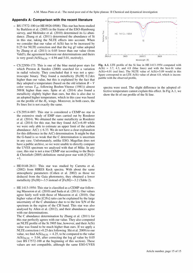
– BS 17572-100 (or HE 0926-0508): This star has been studiedby Barklem et al. (2005) in the frame of the ESO-Hambourgsurvey, and Meléndez et al. (2010) determined its Li abun-dance. Zhang et al. (2011) determined the abundance of Siin this star, taking the NLTE effects into account. Whenwe consider that our value of A(Si) has to be increased by0.25 for NLTE correction and that the log gf value adoptedby Zhang et al. (2011) is 0.05 lower than our value (fromVald3), the agreement between our determinations and theirsis very good (A(Si)NLTE = 4.94 and 5.01, rectively).

– CS 22950-173: This is one of the blue metal-poor stars forwhich Preston & Sneden (2000) searched for a variationin radial velocity. They concluded that it was not a spec-troscopic binary. They found a metallicity [Fe/H] 0.2 dexhigher than our value, but this is explained by the fact thatthey adopted a temperature (based on the old relation B − Vcolor versus Teff , following Boehm-Vitense (1981)) almost500 K higher than ours. Spite et al. (2014) also found ametallicity slightly higher than ours, but this is also due toan adopted higher temperature, which in this case was basedon the profile of the Hα wings. Moreover, in both cases, theFe lines list is not exactly the same.

– CS 29514-007: This star is considered a CEMP-no star inthe extensive study of EMP stars carried out by Roedereret al. (2014). We obtained the same metallicity as Roedereret al. (2014) for this star, but they found A(C)=6.49 whilewe were only able to estimate an upper limit of the carbonabundance: A(C) ≤ 6.33. We do not have a clear explanationfor this difference in the A(C) determination. It might be thatthe G-band is so weak that the C determination is uncertainin any case. Unfortunately, unlike ESO, Magellan does nothave a public archive, so we were unable to directly comparethe UVES spectrum we analysed with that of Mike. In anycase, this star is not a true CEMP star according to the Beers& Christlieb (2005) definition: metal-poor star with [C/Fe]>+1.

– HE 0148-2611: This star was studied by Carretta et al.(2002) from HIRES Keck spectra. With about the sameatmospheric parameters (Cohen et al. 2002) as those wededuced from the Gaia photometry, they obtained a lowermetallicity [Fe/H]=–3.5 instead of [Fe/H]=–3.2 (Table 2).

– HE 1413-1954: This star is classified as a CEMP star follow-ing Masseron et al. (2010) and Suda et al. (2011). Our valuesagree fairly well with those of Masseron et al. (2010). Ourhigher value of the [C/Fe] ratio can be explained by the largeuncertainty of the C abundance due to to the low S/N of thespectrum in the region of the CH band. This star was alsoanalysed by Allen et al. (2012), and their abundances agreewith our determinations.The C abundance determination by Zhang et al. (2011) forthis star perfectly agrees with our value. They also computedan NLTE profile of the Si 3905 line, however, and their A(Si)value was found to be much higher than ours. If we apply aNLTE correction (+0.25 dex following Shi et al. 2009) to ourvalue, we find A(Si)NLTE = 4.25, to be compared to the valueA(Si)NLTE = 5.04, after correcting the log gf value by 0.05(see BS 17572-100 at the beginning of this section). Thesevalues are not compatible, although the same ESO-UVES

Fig. A.1. LTE profile of the Si line in HE 1413-1954 computed withA(Si) = 3.7, 4.3, and 4.8 (blue lines) and with the best-fit valueA(Si)=4.01 (red line). The NLTE value of A(Si)=5.09 would in thisfigure correspond to an LTE A(Si) value of about 4.8, which is incom-patible with the observed profile,

spectra were used. The slight difference in the adopted ef-fective temperature cannot explain this effect. In Fig A.1, weshow the fit of our profile of the Si line.


Documents

The metal-poor end of the Spite plateau: II Chemical and