The Measurement of Precipitable Water Vapor Over Texas

Using the Global Positioning System

by

David Owen Whitlock

March 2000

Center for Space ResearchThe University of Texas at Austin

CSR-TM-00-03

This work was supported by theTexas Higher Education Board Advanced Technology Program

Center for Space ResearchThe University of Texas at Austin

Austin, Texas 78712

Supervised by:Robert S. Nerem

The Measurement of Precipitable Water Vapor Over Texas

Using the Global Positioning System

The goal of this experiment was to demonstrate that the Global Positioning System (GPS)

can be a fast, accurate, and inexpensive method to measure atmospheric precipitable

water vapor (PWV). Data from a network of up to 20 GPS receivers were processed to

measure PWV in near real time (approximately one hour) over the state of Texas. 16

permanent GPS antennas from the Continuously Operating Reference Stations network

(which encompasses sites operated by the Forecast Systems Laboratory, United States

Coast Guard, Federal Aviation Administration/National Travel Safety Board, and the

International GPS Service) as well as four new GPS antennas and receivers (set up by the

Center for Space Research within the state of Texas) were utilized to gather the data. The

four Trimble antennas and receivers were installed as part of this investigation in Austin,

Brownwood, Laredo, and Wichita Falls, Texas. Paroscientific MET3 meteorological

sensors were installed with the GPS equipment to measure surface pressure and

temperature, both of which are necessary to extract PWV from GPS data. GPS data were

gathered hourly from all available sites, then processed using the Jet Propulsion

Laboratory's GIPSY-OASIS II software to estimate the total atmospheric delay of the

GPS signal in the zenith direction. This signal can be converted to PWV with knowledge

of the aforementioned surface atmospheric conditions. The output from this processing

were near real time maps showing PWV over Texas and its surrounding states and time

series of PWV, pressure, and temperature at each individual GPS site.

Table of Contents

CHAPTER 1 - INTRODUCTION. . . . . . . . . . . . . . . . . . . . . . . . . . . . . . . . . . . . . . . . . . . . . . . . . . . . . . . . . . . . . 1

THE GLOBAL POSITIONING SYSTEM .................................................................................. 1Signals...................................................................................................................... 2Observables................................................................................................................ 3

DEFINITION OF PRECIPITABLE WATER VAPOR .................................................................... 4HISTORICAL TECHNIQUES FOR MEASURING WATER VAPOR.................................................. 5

Radiosonde................................................................................................................. 5Water Vapor Radiometer ............................................................................................... 7The Global Positioning System..................................................................................... 9

MOTIVATION FOR PWV MEASUREMENT............................................................................ 9Utility in Weather Forecasting..................................................................................... 10Utility in Climate Monitoring..................................................................................... 10

PREVIOUS EXPERIMENTATION........................................................................................ 11UNAVCO Colorado Campaign.................................................................................... 11Westford Water Vapor Experiment (WWAVE) ................................................................ 12Gradient and Line of Sight Measurements ...................................................................... 13

HOW THE ATMOSPHERE AFFECTS THE GPS SIGNAL........................................................... 14The Atmosphere........................................................................................................ 14The Effect on the GPS Signal...................................................................................... 16

CHAPTER 2 – THEORY OF ATMOSPHERIC DELAY. . . . . . . . . . . . . . . . . . . . . . . . . . . . . . . . . 1 9

THE PHYSICAL EFFECTS OF THE TROPOSPHERE ON THE GPS SIGNAL ................................... 19Excess Path Length ................................................................................................... 19Refractivity .............................................................................................................. 20

HOW GPS CAN BE USED TO MEASURE WATER VAPOR....................................................... 21Basics of the Signal Delay .......................................................................................... 21Separation of Wet Delay from the Hydrostatic Delay........................................................ 22Mapping the Delay to the Zenith.................................................................................. 23Calculation of PWV from Zenith Delay......................................................................... 26

ERRORS IN MEASURING WATER VAPOR........................................................................... 27GPS Orbits .............................................................................................................. 27Multipath Errors ....................................................................................................... 28WVR Errors ............................................................................................................. 30Pressure Sensor Errors................................................................................................ 31Total Errors.............................................................................................................. 31

CHAPTER 3 – THE GPS NETWORK AND COMPUTATIONAL PROCEDURE . . . 3 2

THE GPS NETWORK...................................................................................................... 32GPS SITE INSTALLATION............................................................................................... 34

Site Requirements ..................................................................................................... 35Hardware for Each CSR Installed Site............................................................................ 35Antenna Installation................................................................................................... 36Receiver and PC Set Up ............................................................................................. 38Firmware Configuration ............................................................................................. 39

COMPUTATIONAL PROCEDURE....................................................................................... 39Downloading GPS Data.............................................................................................. 41Daily Station Position Runs ....................................................................................... 43Estimation Background............................................................................................... 43Tropospheric Delay Estimation.................................................................................... 45Post-GIPSY-OASIS Processing................................................................................... 48

CHAPTER 4 - WATER VAPOR RESULTS. . . . . . . . . . . . . . . . . . . . . . . . . . . . . . . . . . . . . . . . . . . . . . . 5 0

NEAR REAL TIME RESULTS............................................................................................ 51Time Series of Maps.................................................................................................. 51Time Series of PWV, Temperature, and Pressure............................................................. 60Discussion of Near Real Time Results .......................................................................... 65

EFFECT OF ORBIT ACCURACY ON PWV ........................................................................... 66Orbit and Polar Motion Data ....................................................................................... 66Orbit Comparison Results .......................................................................................... 67Orbit Data Comparison .............................................................................................. 70One Day Predicted Orbits vs. Precise Orbits ................................................................... 71Two Day Predicted Orbits vs. Precise Orbits................................................................... 72Discussion of Orbit Comparison Results ....................................................................... 73

COMPARISON TO RADIOSONDE MEASURED PWV .............................................................. 73Radiosonde Comparison Results .................................................................................. 74Radiosonde Data Comparison ...................................................................................... 76Discussion of Radiosonde Comparison Results ............................................................... 77

PROBLEMS AND DELAYS IN PROCESSING......................................................................... 78CORS Downloading.................................................................................................. 78Orbit Download ........................................................................................................ 79CSR Machine Delays................................................................................................. 79Summary of Near Real Time Application ...................................................................... 80

CATASTROPHIC ERRORS ............................................................................................... 81Station Position File Errors ........................................................................................ 81Orbit Errors.............................................................................................................. 82Computation Load and Network Errors.......................................................................... 83

CHAPTER 5 - CONCLUSIONS . . . . . . . . . . . . . . . . . . . . . . . . . . . . . . . . . . . . . . . . . . . . . . . . . . . . . . . . . . . . . 8 4

ACCURACY AND WEATHER MODELING............................................................................ 84FUTURE WORK............................................................................................................. 85

Azimuth and Gradient Water Vapor Calculation............................................................... 85Increase the Network.................................................................................................. 86Dual Frequency......................................................................................................... 86

APPENDIX A. . . . . . . . . . . . . . . . . . . . . . . . . . . . . . . . . . . . . . . . . . . . . . . . . . . . . . . . . . . . . . . . . . . . . . . . . . . . . . . . . . . 8 7

BIBLIOGRAPHY . . . . . . . . . . . . . . . . . . . . . . . . . . . . . . . . . . . . . . . . . . . . . . . . . . . . . . . . . . . . . . . . . . . . . . . . . . . . . . . 8 9

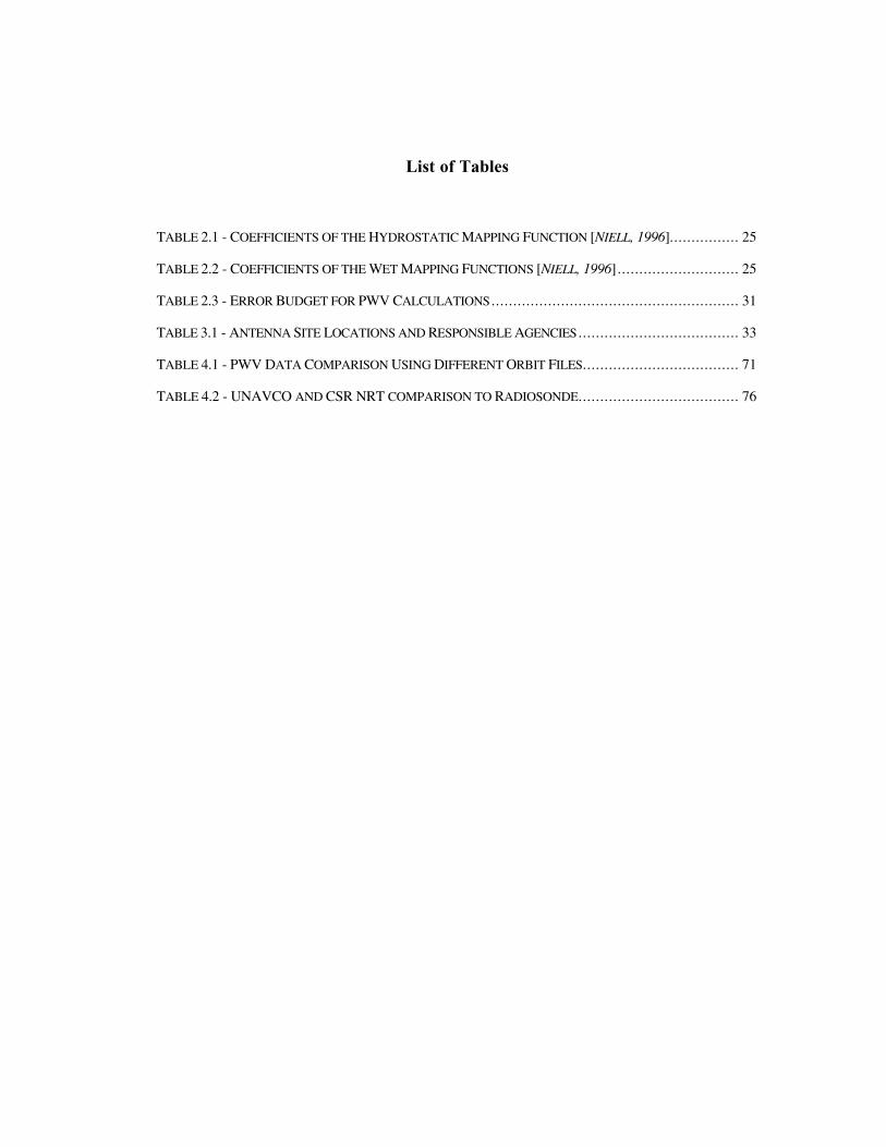
List of Tables

TABLE 2.1 - COEFFICIENTS OF THE HYDROSTATIC MAPPING FUNCTION [NIELL, 1996]................ 25

TABLE 2.2 - COEFFICIENTS OF THE WET MAPPING FUNCTIONS [NIELL, 1996]............................ 25

TABLE 2.3 - ERROR BUDGET FOR PWV CALCULATIONS......................................................... 31

TABLE 3.1 - ANTENNA SITE LOCATIONS AND RESPONSIBLE AGENCIES..................................... 33

TABLE 4.1 - PWV DATA COMPARISON USING DIFFERENT ORBIT FILES.................................... 71

TABLE 4.2 - UNAVCO AND CSR NRT COMPARISON TO RADIOSONDE..................................... 76

List of Figures

FIGURE 1.1 – ALTITUDE RANGE FOR VARIOUS LAYERS OF THE ATMOSPHERE ........................... 15

FIGURE 1.2 – INCREASED SIGNAL DELAY FOR LOWER ELEVATION SATELLITES ......................... 18

FIGURE 2.1 – MULTIPATH COHERENCE FOR FIVE SEPARATE DAYS [ROCKEN ET AL., 1993] ......... 30

FIGURE 3.1 - MAP OF GPS RECEIVER LOCATIONS [WHITLOCK ET AL., 1999]............................. 34

FIGURE 3.2 - LEVELING PLATE (BRWD)............................................................................... 37

FIGURE 3.3 - COMPLETE ANTENNA WITH RAYDOME (BRWD).................................................. 37

FIGURE 3.4 - HARDWARE CONFIGURATION.......................................................................... 38

FIGURE 3.5 - PROCESSING FLOW DIAGRAM FOR ANY HOUR OF DAY 1 (GMT)........................... 40

FIGURE 3.6 - DATA FLOW DIAGRAM FOR CSR SITES............................................................. 42

FIGURE 4.1 - NEAR REAL TIME MAPS.................................................................................. 52

FIGURE 4.1 - NEAR REAL TIME MAPS (CONTINUED)............................................................... 53

FIGURE 4.1 - NEAR REAL TIME MAPS (CONTINUED)............................................................... 54

FIGURE 4.1 - NEAR REAL TIME MAPS (CONTINUED)............................................................... 55

FIGURE 4.1 - NEAR REAL TIME MAPS (CONTINUED)............................................................... 56

FIGURE 4.1 - NEAR REAL TIME MAPS (CONTINUED)............................................................... 57

FIGURE 4.1 - NEAR REAL TIME MAPS (CONTINUED)............................................................... 58

FIGURE 4.1 - NEAR REAL TIME MAPS (CONTINUED)............................................................... 59

FIGURE 4.2 - DAY 2/26/00 TIME SERIES (ARP3).................................................................... 61

FIGURE 4.2 - DAY 2/26/00 TIME SERIES (CSR1).................................................................... 62

FIGURE 4.2 - DAY 2/26/00 TIME SERIES (PATT).................................................................... 63

FIGURE 4.2 - DAY 2/26/00 TIME SERIES (WTFL)................................................................... 64

FIGURE 4.3 - ORBIT COMPARISON FOR FIVE SITES - 2/26/00................................................... 68

FIGURE 4.3 - ORBIT COMPARISON FOR FIVE SITES - 2/26/00 (CONTINUED) ............................... 69

FIGURE 4.3 - ORBIT COMPARISON FOR FIVE SITES - 2/26/00 (CONTINUED) ............................... 70

FIGURE 4.4 - RAPIDLY CHANGING PWV; NRT VS. RADIOSONDE COMPARISON ........................ 74

FIGURE 4.5 - STEADY PWV; NRT VS. RADIOSONDE COMPARISON.......................................... 75

1

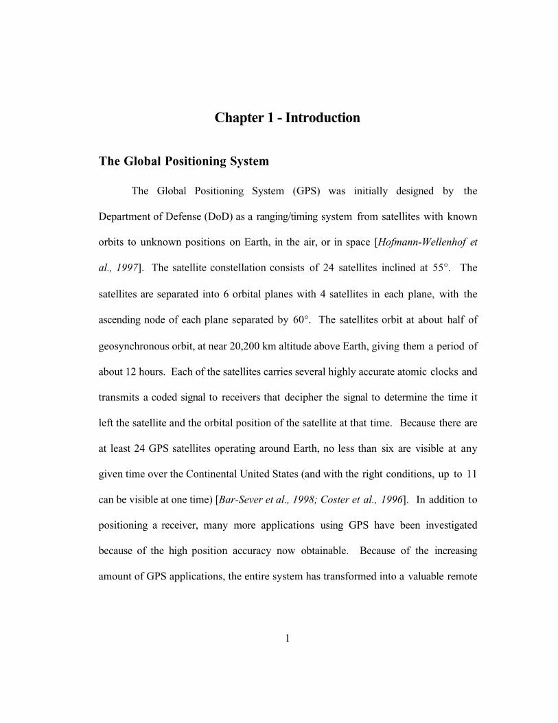
Chapter 1 - Introduction

The Global Positioning System

The Global Positioning System (GPS) was initially designed by the

Department of Defense (DoD) as a ranging/timing system from satellites with known

orbits to unknown positions on Earth, in the air, or in space [Hofmann-Wellenhof et

al., 1997]. The satellite constellation consists of 24 satellites inclined at 55°. The

satellites are separated into 6 orbital planes with 4 satellites in each plane, with the

ascending node of each plane separated by 60°. The satellites orbit at about half of

geosynchronous orbit, at near 20,200 km altitude above Earth, giving them a period of

about 12 hours. Each of the satellites carries several highly accurate atomic clocks and

transmits a coded signal to receivers that decipher the signal to determine the time it

left the satellite and the orbital position of the satellite at that time. Because there are

at least 24 GPS satellites operating around Earth, no less than six are visible at any

given time over the Continental United States (and with the right conditions, up to 11

can be visible at one time) [Bar-Sever et al., 1998; Coster et al., 1996]. In addition to

positioning a receiver, many more applications using GPS have been investigated

because of the high position accuracy now obtainable. Because of the increasing

amount of GPS applications, the entire system has transformed into a valuable remote

2

sensing system in addition to its original use as a navigation tool [Bar-Sever et al.,

1998].

Signals

Each satellite transmits coded data on two frequencies, L1 (1575.42 MHz) and

L2 (1227.6 MHz) [Chen and Herring, 1997; Coster et al., 1996; Hofmann-Wellenhof

et al., 1997; Juan et al., 1997; Ruffini et al., 1998; Ware et al., 1997]. Two distinct

codes, Course-Acquisition (C/A) code and Precision (P) code, are superimposed on

the carrier frequencies, along with satellite ephemerides, system time, satellite clock

corrections, ionospheric modeling coefficients, and satellite status (health)

information.

The C/A code (also known as the Standard Positioning Service) is a

pseudorandom noise (PRN) code that is broadcast on the L1 carrier only. During

initial experimentation, the C/A code produced point-positioning accuracies much

better than expected, so the DoD introduced Selective Availability (SA) to deny this

high accuracy to unauthorized users. SA dithers the clock and satellite position

information to limit accuracy to approximately 100 m in the horizontal direction, and

150 m in the vertical direction.

The P code (also known as the Precise Positioning Service) is a PRN code

transmitted on both the L1 and L2 carrier frequencies, which allows for first order

removal of ionospheric errors. To reserve precise positioning for DoD use, the P code

3

is almost always encrypted to what is referred to as Y code. The Y code is a

combination of the P code and an encryption code called the W code. This protection

of the P code is called Anti-Spoofing, or A-S. A-S is either on or off; there is no

variable effect.

Observables

A pseudorange, or measured range from satellite to receiver, is derived from

the broadcast signal. If four or more satellite signals are received simultaneously, an

approximate three-dimensional position and correction to the less accurate receiver

clock are calculated by the receiver in real time. Because the transmit time and receive

time are different, true range cannot be measured. The pseudorange is derived from

the equation

ρ ρ δ δ= + −( )true r tc (1.1)

where ρ is the observed pseudorange calculated from the light-time equation, ρtrue is

the difference of position of the receiver at the true receive time and the satellite at the

true transmit time, and δt and δr represent the bias created by clock errors in the

satellite and receiver.

Another observable is the carrier phase of the signal, which does not look at

the actual information on the signal, but only the phase of the signal. The carrier

phase is defined by

4

ρ ρ δ δ λφ = + −( ) +true r tc N (1.2)

where

ρ λ φ λφ = − =∆ ΦSR

(1.3)

where the fractional beat phase of the signal is converted into a pseudorange by

scaling with the wavelength, λ. ρtrue and the clock corrections remain the same as for

the code pseudorange definition. The integer number of cycles, N, is unique for each

receiver-satellite combination and is typically not known. Once a receiver has locked

onto a satellite signal, only the fractional beat phase changes while N remains

constant. N, known as the integer ambiguity, can be solved for using the code

pseudoranges, or estimated. If a receiver loses signal lock on a satellite, a new integer

ambiguity must be solved for once the lock is re-established. The use of carrier phase

data can improve the accuracy of positioning to sub-centimeter precision [Blewitt,

1990; Dong and Bock, 1989]

Definition of Precipitable Water Vapor

Precipitable water vapor is defined as the height of liquid water that would

result from condensing all the water vapor in a column from the surface of Earth to the

top of the atmosphere [Bevis et al., 1992; Coster et al., 1996]. PWV is typically

calculated in centimeters or millimeters and is a measure of the amount of water vapor

5

that can be found in the lower atmosphere over a given location. PWV is highly

varying in both space and time.

Historical Techniques for Measuring Water Vapor

Atmospheric precipitable water vapor is not easy to measure in near real time,

primarily because of the difficulty in placing instrumentation where knowledge of

PWV is desired. Outside of GPS, radiosondes and water vapor radiometers are the

industry standard in measuring PWV, although both show many weaknesses,

especially in spatial and temporal resolution.

Radiosonde

A radiosonde is a balloon-launched instrument package that measures

atmospheric conditions above the surface of Earth [Bevis et al., 1996; Bevis et al.,

1992]. They are implemented in a geographical location for which meteorological

characteristics of the troposphere are desired to be known. Radiosondes ascend

through the atmosphere slowly, while communicating atmospheric conditions back to

the ground through a radio communications link.

There are several advantages to using radiosondes to measure water vapor in

the atmosphere. First, the radiosonde measurements can be gathered nearly

anywhere. True humidity, temperature, and pressure values can be obtained without

tedious processing of the data. Finally, since radiosondes have been utilized for many

6

years, they are proven to be reliable and their data are known to be dependable and

accurate.

Unfortunately, there are several drawbacks to the use of radiosondes. Because

of the fundamental nature of balloon-borne instrumentation, the equipment can only

be used once. This makes the use of radiosondes very cost inefficient [Bevis et al.,

1992; Coster et al., 1996]. In fact, most current geographical locations with regular

radiosonde launches are considering a reduction in launch frequency due to excessive

cost [Coster et al., 1996]. Also, in near real time applications, radiosondes are not as

useful as other methods. They take approximately one hour to reach the tropopause

(the upper boundary of the lowest layer of the atmosphere), thus providing little data

on a rapid time scale [Coster et al., 1996]. If data are needed for prediction of

inclement or rapidly changing weather, radiosonde measurements are essentially

useless. There is a severe limit on the two-dimensional geographical space that can be

measured using a radiosonde [Bevis et al., 1992; Coster et al., 1996; Rocken et al.,

1993]. Because water vapor varies on a much finer scale than temperature and wind,

radiosonde measurement of water vapor cannot be accurately modeled in two

dimensions [Anthes, 1983]. Once released, data are abundant for the space in which

the radiosonde travels, but not for other locations surrounding that area [Coster et al.,

1996].

7

Water Vapor Radiometer

A water vapor radiometer (WVR) is a radio telescope, either land-borne or

space-borne, that can determine atmospheric conditions by measuring the background

temperature along a given line of sight [Bevis et al., 1992; Hogg et al., 1981; Rocken et

al., 1993; Ware et al., 1993]. Land-based WVRs measure the background radiation in

deep space to measure calculate the water vapor between the ground and space along

the bore site [Bevis et al., 1992]. Space-based WVRs are installed on satellites and

pointed towards Earth. They measure the background temperature of the Earth’s

surface and estimate the atmospheric conditions between the satellite and Earth in that

manner [Bevis et al., 1992]. Space-based WVRs cannot accurately measure

atmospheric conditions over land or cloud cover, because the background temperature

can vary significantly depending on the surface that the radio waves strike. Space-

based WVRs can be quite useful over oceans and large bodies of water, because the

background temperature is nearly uniform on the surface of the water [Bevis et al.,

1996; Bevis et al., 1992; Coster et al., 1996; Rao et al., 1990; Rocken et al., 1993].

For uses in which WVR data are compared to GPS data, the WVR will be

programmed to point toward visible GPS satellites. For a five satellite array, it takes

about eight minutes to look in each satellite direction and gather data [Rocken et al.,

1993; Ware et al., 1997].

8

The advantages of WVRs are that they are mobile and can be placed nearly

anywhere. Some initialization time is needed to calculate calibration coefficients, but

scientists can place WVRs almost anywhere on the surface of Earth and get

measurements with relative ease [Bevis et al., 1992]. Also, they have near real time

capability. Unlike radiosondes, there is no instrument travel time required to make

meteorological measurements. Once calibrated, the WVR can be pointed, line-of-sight

measurements made, and data accumulated very swiftly. Also, as in the use of

radiosondes, WVRs have been utilized for many years and have proven to be a reliable

method for accurate atmospheric data measurement.

WVRs suffer from similar limitations as the radiosonde, including instrument

cost. A single WVR can cost hundreds of thousands of dollars, so any kind of array

of WVRs for use in mapping or data gathering over a significant two-dimensional

space becomes cost-prohibitive [Coster et al., 1996]. This tends to limit the spatial

resolution of atmospheric data, as most research organizations cannot afford one

WVR, let alone several, to provide accurate atmospheric modeling in a two-

dimensional sense [Rocken et al., 1993]. A major disadvantage unique to the WVR is

that no data can be gathered when the weather is extremely overcast or raining [Bevis

et al., 1992; Niell et al., 1996; Ware et al., 1997].

9

The Global Positioning System

In addition to the more obvious uses, such as high-precision geodesy, an

increasing number of applications for GPS are being developed, especially in the fields

of climatology and meteorology [Bar-Sever et al., 1998]. Because the GPS signal

travels through the entire atmosphere, the signal can be processed on the ground and

atmospheric water vapor extracted. The current technologies used to measure

atmospheric water vapor discussed above can be expensive and may provide little

meaningful data, especially in near real time. Because there are many GPS antennas

continuously operating, a significant quantity of water vapor data can be gathered in

near real time using GPS. Chapter 2 will discuss in detail how GPS can be used to

measure PWV.

Motivation for PWV Measurement

Atmospheric water vapor plays a critical role in atmospheric processes that

act on a variety of temporal and spatial scales [Bevis et al., 1992]. Because water

vapor is the most variable major constituent in our atmosphere, near real time

measurement of PWV can help meteorologists better understand how local weather

and climate are changing over time [Bevis et al., 1992].

10

Utility in Weather Forecasting

Limitations in the quantity and accuracy of water vapor data are a major

source of error in daily forecasts of precipitation and inclement weather. Accurate

information regarding the horizontal and vertical distribution of PWV can lead to

significant improvement in daily weather forecasting. GPS receivers distributed over

small spatial scales (less than 500 km) can provide water vapor data that could be

assimilated into numerical weather forecasts [Rocken et al., 1993]. The distribution of

water vapor is closely coupled to the formation of clouds and subsequent rainfall, as

there is an unusually large latent heat associated with water s change of phase, which

can play a critical role in the evolution of storm systems and severe weather [Bevis et

al., 1993; Bevis et al., 1992]. Due to the high temporal and spatial variance of PWV,

mathematical modeling of water vapor to the accuracy needed for weather prediction

is not feasible. Direct measurement remains the only way to gather accurate water

vapor values useful for weather forecasting.

Utility in Climate Monitoring

Water vapor contributes more than any other atmospheric component to the

greenhouse effect [Bevis et al., 1992; Coster et al., 1996]. In order to understand and

predict changes in Earth s climate on a large time scale, long-term measurement of

PWV on a global scale must be carried out. The increasing number of GPS antennas

throughout the United States and the world can provide atmospheric scientists with

11

an abundance of long term data over land for climate studies to compliment existing

WVR and radiosonde measurements, which are more useful over the oceans [Bevis et

al., 1993; Bevis et al., 1992; Yuan et al., 1993].

Previous Experimentation

Several GPS campaigns have been performed to verify the utility and accuracy

of GPS water vapor measurements. Initial experimentation attempted to verify the

accuracy of GPS measured PWV when compared to WVR or radiosonde

measurements. PWV accuracy of 1 mm has been verified during various experiments

and campaigns [Coster et al., 1996; Nam et al., 1996; Niell et al., 1996; Rocken et al.,

1993; Ware et al., 1993]. Recently, more detailed experimentation and analysis has

been done to investigate the feasibility of measuring delays in the individual directions

of the GPS satellites, whereas initial experimentation only estimated water vapor in

the zenith direction.

UNAVCO Colorado Campaign

The University Navstar Consortium (UNAVCO) performed a two-antenna

GPS campaign to determine the accuracy of PWV measurement with GPS from

September 17, 1992 to November 28, 1992 [Rocken et al., 1993; Ware et al., 1993].

Antennas were placed 50 kilometers apart in Boulder and Platteville, Colorado, with a

meteorological sensor and WVR at each receiver location. No radiosonde balloons

12

were used, and PWV data obtained from GPS were compared to the WVR measured

PWV. Because a relatively short baseline was used, PWV was only estimated and

compared to WVR results at Boulder. When using precise GPS orbits, the experiment

showed sub-millimeter accuracy of PWV values obtained with GPS as compared to

PWV values obtained with a WVR. When broadcast orbits were used for satellite

positions, the accuracy decreased by 30% to an accuracy of about 1 mm of PWV.

This level of accuracy using broadcast orbits demonstrated the near real time

capability of PWV measurement with GPS.

Westford Water Vapor Experiment (WWAVE)

11 GPS antennas were placed within a very short baseline of about 25

kilometers to measure the temporal and spatial variability of PWV over the area

surrounding Westford, Massachusetts [Coster et al., 1996; Niell et al. 1996]. The

data were collected from August 15, 1995 to August 30, 1995. Three of the antennas

were placed within a kilometer radius near the center of the network and

meteorological sensors were placed at eight of the sites. The zenith PWV data

gathered were compared to zenith WVR and radiosonde PWV measurements gathered

at the central location. Accuracy of 1-2 mm of PWV was obtained when comparing

the PWV results estimated with GPS with PWV results obtained by WVR and

radiosondes. From GPS site to GPS site, agreement in PWV of less than 1 mm was

obtained, although this high degree of accuracy can be attributed to some identical

13

error sources (such as orbit errors) seen by each of the receivers. Because of the limit

in radiosonde launches, and the lack of utility of WVRs during rain (it rained twice

during the campaign), the quantity of alternatively measured data for comparison was

limited during the WWAVE experiment.

Gradient and Line of Sight Measurements

When calculating zenith delay, which is converted to PWV, symmetry in the

azimuthal direction is a common assumption. This assumption can be far from valid,

especially during the time when weather systems may be approaching an antenna

from a distinct azimuth direction. This asymmetry can be especially important in

atmospheric correction for horizontal and vertical precise-positioning [Bar-Sever et

al., 1998]. Gradient effects can be as high as 5 cm difference in delay at 7° elevation

[MacMillan, 1995]. By modeling this gradient, a horizontal and vertical position

repeatability increase of nearly 20% is obtainable [Bar-Sever et al., 1998]. GPS can

help model azimuth gradients by analyzing the slant-path water vapor along GPS

signal paths. During a three day campaign in May, 1996, 1.3 mm rms agreement was

found when comparing GPS line of sight delays with WVR measurements [Ware et

al., 1997]. During an experiment in Madrid, Spain, gradient estimates obtained with

GPS and a WVR compared favorably, leading to the belief that GPS slant delay

estimation capability is a strong possibility in the near future [Ruffini et al., 1999].

This capability was also demonstrated in Onsala, Sweden during a similar gradient

14

estimate campaign [Bar-Sever et al., 1998]. By removing the assumption of

atmospheric symmetry in the azimuth direction, an improvement positioning and

atmospheric measurement accuracy can be obtained using GPS.

How the Atmosphere Affects the GPS Signal

The Atmosphere

The atmosphere (Figure 1.1) is made up of several layers. Scientists define

these layers by their atmospheric characteristics, such as temperature, pressure, and

humidity [Brunner and Welsch, 1993]. The closest layer to Earth is the troposphere,

which begins at Earth’s surface and extends to between 9 and 16 kilometers above the

surface. The approximately 7 kilometer region between the troposphere and the next

layer, the stratosphere, is called the tropopause. The tropopause has characteristics

of both the troposphere and stratosphere. From 16 kilometers to 50 kilometers above

Earth’s surface is the stratosphere. The troposphere, tropopause, and stratosphere

compose what is referred to as the neutral atmosphere, as it is electrically neutral.

Above the stratosphere, the atmosphere is electrically charged and called the

ionosphere. From about 50 kilometers to about 80 kilometers is the mesosphere,

which is the lower ionosphere. Outside the mesosphere is the remainder of the

ionosphere, which extends from about 80 kilometers above the surface to the upper

reaches of the atmosphere (extending even beyond 1000 km). Each of these

15

atmospheric regions adversely affects the GPS signal by delaying its arrival at Earth’s

surface by a finite amount of time.

Ionosphere

80 Kilometers

Ionosphere/Mesosphere

50 Kilometers

Stratosphere

16 Kilometers

Tropopause

9 Kilometers

Troposphere

0 Kilometers

Figure 1.1 — Altitude Range for Various Layers of the Atmosphere

16

The Effect on the GPS Signal

The delay of the atmosphere can cause significant errors for precise-

positioning applications. The ionospheric signal delay is dispersive in nature in that

the delay is dependent upon the frequency of the signal [Hofmann-Wellenhof et al.,

1997]. Because GPS broadcasts on two separate frequencies, this error can be

eliminated by the mathematical combination of the two separate frequency signals.

The focus of the research discussed here will be the delay caused by the troposphere,

or neutral atmosphere. Unlike the ionosphere, the delay caused by the troposphere is

non-dispersive, or completely independent of the signal frequency. However, with

accurate knowledge of GPS antenna location and GPS satellite location, the signal

delay errors caused by the troposphere can be measured. Atmospheric delay caused

by the troposphere is typically computed in length. For example, a standard zenith

tropospheric delay would be about 2.3 meters, meaning that the troposphere caused a

GPS receiver to read an extra 2.3 meters distance between itself and a fictitious

satellite at zenith [Bevis et al. 1996; Chen and Herring, 1997].

The delay caused by the troposphere can be categorized into two components,

the hydrostatic delay and the wet delay [Bar-Sever et al., 1998; Bevis et al., 1996;

Bevis et al., 1992; Coster et al., 1996; Gregorius and Blewitt, 1998; Hofmann-

Wellenhof et al., 1997; Rocken et al., 1993; Ware et al., 1997; Yuan et al., 1993]. The

hydrostatic delay is caused by dry gases in the troposphere and the non-dipole

17

component of water refractivity while the wet delay is caused solely by the dipole

component of water refractivity, which we refer to as water vapor [Bar-Sever et al.,

1998]. The hydrostatic delay makes up almost 95% of the total tropospheric delay

and typically does not vary more than 0.5% over the course of a day [Bevis et al.,

1996]. This delay is dependent on the atmospheric pressure and can be estimated by

utilizing the surface pressure on Earth. If surface pressure is known to 0.4 mbar, then

the hydrostatic delay can be estimated within the accuracy of 1 millimeter using well

known models, such as the Saastamoinen model [Bevis et al., 1996; Nam et al., 1996;

Rocken et al., 1993]. The wet delay, however, cannot be estimated using surface

atmospheric measurements. By estimating the total zenith delay, then calculating the

hydrostatic delay from surface pressure, the remaining delay is caused by water vapor

in the atmosphere.

As discussed in the previous section, initial experimentation is being done to

estimate line-of-sight delays in the individual directions to the GPS satellites.

However, in general, mapping functions are used to take signal delays from each

individual GPS satellite and map them to the zenith direction to estimate only one

zenith signal delay, or the delay in signal transmission (measured in length) a GPS

satellite would experience were it at zenith over the GPS antenna. Mapping functions

used for this purpose will be discussed in the next chapter. Of the 2.3 m approximate

zenith delay, about 2.2 m is caused by hydrostatic atmospheric characteristics and

18

approximately 10 cm of range error is caused by water vapor [Bevis et al., 1996; Bevis

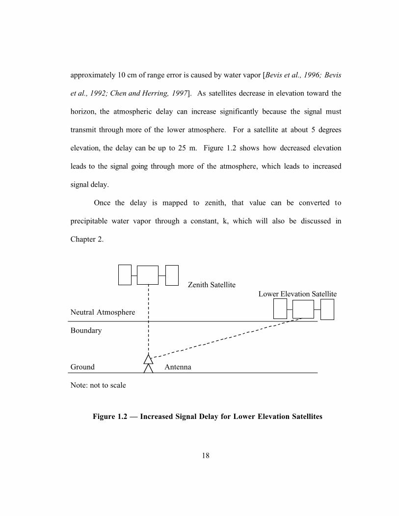
et al., 1992; Chen and Herring, 1997]. As satellites decrease in elevation toward the

horizon, the atmospheric delay can increase significantly because the signal must

transmit through more of the lower atmosphere. For a satellite at about 5 degrees

elevation, the delay can be up to 25 m. Figure 1.2 shows how decreased elevation

leads to the signal going through more of the atmosphere, which leads to increased

signal delay.

Once the delay is mapped to zenith, that value can be converted to

precipitable water vapor through a constant, k, which will also be discussed in

Chapter 2.

Zenith Satellite

Lower Elevation Satellite

Neutral Atmosphere

Boundary

Ground Antenna

Note: not to scale

Figure 1.2 — Increased Signal Delay for Lower Elevation Satellites

19

Chapter 2 — Theory of Atmospheric Delay

The Physical Effects of the Troposphere on the GPS Signal

The neutral, lower atmosphere has two effects on a GPS signal. The first

effect is the delay of the signal due to the troposphere. The second effect is to refract

the GPS signal. The GPS signal will travel on a curved path instead of a straight line.

Both of these effects are due to the changing refractivity of the lower atmosphere in

the ray path of the GPS signal. [Bevis et al., 1992; Yuan et al., 1993]

Excess Path Length

The excess path length is given by the path integral [Bevis et al., 1992; Yuan et

al., 1993]

∆L n s ds GL

= ( ) −∫ (2.1)

where n(s) is the refractive index as a function of position, s, along the path L and G is

the straight line geometric path length through the atmosphere.

Simplified, Equation 2.1 can be expressed as [Bevis et al., 1992; Yuan et al.,

1993]

20

∆L n s ds S GL

= ( ) −[ ] + −[ ]∫ 1 (2.2)

where S is the path length along L.

This separates the change in travel length into the first term, which is the delay

due to the slowing effect of the troposphere and the second term, which is the added

path length due to the bending of the signal. For most elevations over 15°, S — G is

less than a centimeter, meaning the first term is the bulk of the excess length.

Refractivity

It is mathematically easier to use the atmospheric refractivity, N, instead of

refractive index, n, in Equation 2.2 utilizing the relation [Bevis et al., 1992; Yuan et al.,

1993]

N n= −( )10 16(2.3)

where N can be related empirically to temperature, T, pressure, P and water vapor

pressure Pv by [Hofmann-Wellenhof et al., 1997; Smith and Weintraub, 1953]

NP

T

P

Tv=

+

77 6 3 73 105

2. . * (2.4)

or a more accurate and complex representation [Thayer, 1974]

21

N kP

TZ k

P

TZ k

P

TZd

dv

vv

v=

+

+

− − −1

12

13 2

1 (2.5)

in which k1 = (77.604 ± 0.014) K/mbar, k2 = (64.79 ± 0.08) K/mbar, k3 = (3.776 ±

0.004) K2/mbar, Pd is the partial pressure of dry air (in mbar), and Zd

-1 and Zv

-1 are

inverse compressibility factors for dry air and water vapor.

Because of the extreme difficulty in finding values for many of the parameters

in Equations 2.4 and 2.5, the total atmospheric delay is divided into a hydrostatic

delay and a wet delay [Saastamoinen, 1972]. This method of dividing the delay is

ideal for utilizing GPS to measure atmospheric water vapor.

How GPS Can be Used to Measure Water Vapor

Basics of the Signal Delay

For a given measured distance from the ground to the satellite (using both

pseudorange and carrier phase from Equations 1.1 and 1.2), the difference between the

measured range and the actual range can be extremely simplified to

R i t= + +ρ ε ε (2.6)

ε ε εt h w= + (2.7)

where R is the measured range from GPS antenna, ρ is actual range, εi is the

ionospheric error, εt is the tropospheric error , εw is the wet delay error, and εh is the

22

hydrostatic delay. If the satellite orbit and receiver location are known to a good

degree of accuracy, then an estimate of ρ is known. εi can be estimated due to the

frequency dependent nature of the ionospheric delay using a mathematical

combination of the two GPS frequencies. Then, we compute εh from the atmospheric

measurements and measure R from the GPS data leaving the only unknown to be the

error caused by the wet component of the atmosphere, εw.

Separation of Wet Delay from the Hydrostatic Delay

The hydrostatic delay is the cause of the bulk of the total GPS signal delay

due to the troposphere. It can be accurately estimated by measuring local surface

pressure and using the formula [Bevis et al., 1992; Yuan et al., 1993]

∆L ZHDP

f hhs= = ±( ) ( )

−10 2 2779 0 00246 . .,λ

(2.8)

where Ps is surface pressure in mbar and f(λ,h) is the station latitude and height

dependent gravitation function [Bevis et al., 1992]

f h hλ λ, . * cos .( ) = − −( )1 0 00266 2 0 00028 (2.9)

and is close to unity. The wet delay varies much more in time and space than the

hydrostatic delay. It is also much more difficult to measure using atmospheric data

23

exclusively. The formula for calculating it is [Bevis et al., 1996; Bevis et al., 1992;

Yuan et al., 1993]

∆L ZWD kP

Tdz k

P

Tdzw

v v= = +

− ∫∫10 62 3 2'

(2.10)

in which k2 = (17 ± 10) K/mbar, k3 = (3.776 ± 0.03)*105 K

2/mbar (same as Equation

2.5), Pv is the partial pressure of water vapor (only available through radiosondes),

and T is the temperature (K)

Since the integral of the partial pressure cannot be measured in near real time,

it is easier to measure the total delay from GPS measurements, then correct it using

the much more easily calculable hydrostatic delay. The remaining portion of the total

delay is the wet delay.

Mapping the Delay to the Zenith

For GPS measurement of zenith precipitable water vapor, the signal delay in

each direction to each GPS satellite is not generally estimated individually. Instead,

the individual delays are mapped from each individual satellite direction to a single

zenith delay. This mapping method assumes that the delay is independent of

azimuth. However, it does not assume that the delay is independent of elevation.

This assumption could never be made, because of the significant increase in delay that

is seen when the signal travels through much more of the atmosphere at lower

24

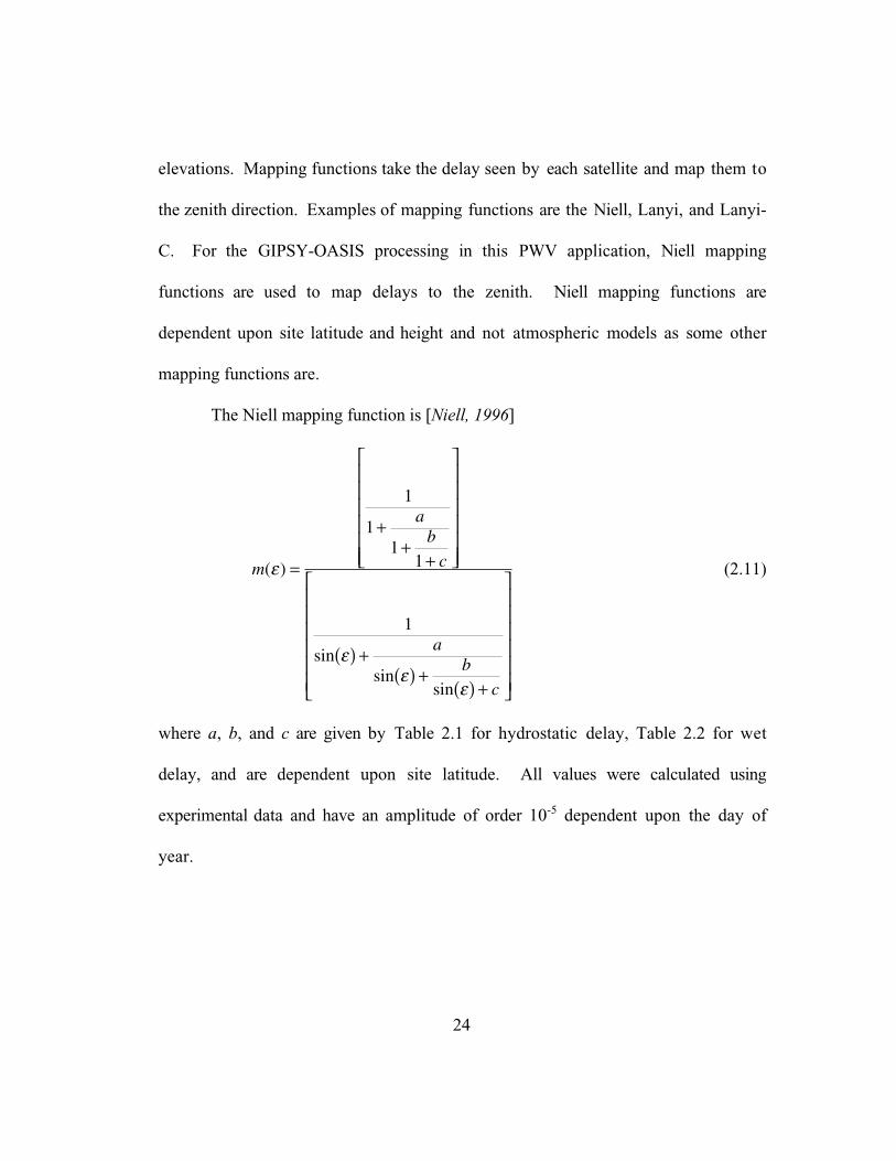
elevations. Mapping functions take the delay seen by each satellite and map them to

the zenith direction. Examples of mapping functions are the Niell, Lanyi, and Lanyi-

C. For the GIPSY-OASIS processing in this PWV application, Niell mapping

functions are used to map delays to the zenith. Niell mapping functions are

dependent upon site latitude and height and not atmospheric models as some other

mapping functions are.

The Niell mapping function is [Niell, 1996]

m

ab

c

ab

c

( )

sinsin

sin

ε

εε

ε

=

++

+

( ) +( ) +

( ) +

1

11

1

1

(2.11)

where a, b, and c are given by Table 2.1 for hydrostatic delay, Table 2.2 for wet

delay, and are dependent upon site latitude. All values were calculated using

experimental data and have an amplitude of order 10-5

dependent upon the day of

year.

25

Latitude (all values are 10-3

)

Coefficient 15° 30° 45° 60° 75°

a 1.2769934 1.2683230 1.2465397 1.2196049 1.2045996

b 2.9153693 2.9152299 2.9288445 2.9022656 2.9024912

c 62.610505 62.837393 63.721774 63.824265 64.258455

Table 2.1 - Coefficients of the Hydrostatic Mapping Function [Niell, 1996]

Latitude (all values are 10-4

)

Coefficient 15° 30° 45° 60° 75°

a 5.8021897 5.6794847 5.8118019 5.9727542 6.1641693

b 14.275268 15.138625 14.572752 15.007428 17.599082

c 434.72961 467.29510 439.08931 446.26982 547.36038

Table 2.2 - Coefficients of the Wet Mapping Functions [Niell, 1996]

The mapping function is adjusted for the height above geoid with [Niell, 1996]

dm

dhf a b cht ht ht

εε

ε( ) =( )

− ( )1sin

, , , (2.12)

where f is Equation 2.11 for

a E

b E

c E

ht

ht

ht

= −= −= −

2 53 5

5 49 3

1 14 3

.

.

.

giving a mapping function height correction of [Niell, 1996]

26

∆mdm

dhHε ε( ) = ( )

(2.13)

where H is the height of the site above geoid.

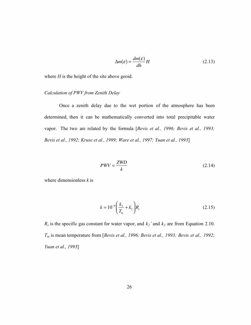
Calculation of PWV from Zenith Delay

Once a zenith delay due to the wet portion of the atmosphere has been

determined, then it can be mathematically converted into total precipitable water

vapor. The two are related by the formula [Bevis et al., 1996; Bevis et al., 1993;

Bevis et al., 1992; Kruse et al., 1999; Ware et al., 1997; Yuan et al., 1993]

PWVZWD

k= (2.14)

where dimensionless k is

kk

Tk R

mv= +

−10 6 32'

(2.15)

Rv is the specific gas constant for water vapor, and k2’ and k3 are from Equation 2.10.

Tm is mean temperature from [Bevis et al., 1996; Bevis et al., 1993; Bevis et al., 1992;

Yuan et al., 1993]

27

T

P

Tdz

P

Tdz

m

v

v=

∫∫ 2

(2.16)

which again is difficult to calculate because of the near impossible task of measuring

the values to integrate. However, the mean temperature has been estimated linearly

[Bevis et al., 1993; Bevis et al., 1992; Yuan et al., 1993]:

T Tm s≅ +70 2 0 72. . (2.17)

where Ts is surface temperature in Kelvin.

Tm has an rms deviation of 4.7 K which contributes to errors in the

measurement of PWV with GPS, but not significantly, as the dependence upon

temperature is weak [Bevis et al., 1996].

Errors in Measuring Water Vapor

Error estimations for PWV measurement using GPS have been performed

previously and this section summarizes these results.

GPS Orbits

GPS orbit errors affect the calculation of receiver-satellite range in Equation

2.6. There are several different levels of accuracy of GPS orbits produced by various

centers around the world (e.g. Jet Propulsion Laboratory, International GPS Service,

GeoForschungsZentrum). First, there are predicted orbits, which are satellite

28

positions extrapolated into the future. These orbits decrease in accuracy from less

than 1 m up to 3 m in satellite position after three days [Gregorius, 1996]. Predicted

orbits are primarily used for near real time applications. Secondly, a slightly more

accurate, quick-time , orbit is available about a day after data is gathered. These

orbits, which are accurate to about 30 - 45 cm, can be used to post-process GPS data

within a few days after they are gathered. Thirdly, in about ten days to two weeks,

the satellites are calculated to their most precise positions, which can then be used for

precise GPS applications. The precise orbits are accurate to 10 - 20 cm.

In addition to these calculated or extrapolated orbits, there are orbit data

broadcast by the GPS satellites that can be used for real time positioning and near real

time geodetic measurements. These orbits, with SA implemented, have accuracy

which allow positioning to only within 100 m horizontal in real time [Hofmann-

Wellenhof et al., 1997].

Orbit errors of 1 in 100 million (centimeter level errors in satellite location)

yield an error of approximately 0.1 mm error in PWV [Rocken et al., 1993; Ware et al.

1997]. For predicted orbit error of 1 m, the PWV error jumps to 1 - 3 mm.

Multipath Errors

Multipath errors affect the measurement of pseudorange and carrier phase in

Equation 2.6. Multipath occurs when a GPS signal reflects off of another surface,

thus reaching the receiver by more than one path [Hofmann-Wellenhof et al., 1997;

29

Rocken et al., 1993]. Multipath is best reduced by antenna design, site location, and

data processing. Most antennas used in precise-positioning have a choke ring, which

helps mitigate multipath. Also, by not locating the antenna near tall buildings or other

reflective surfaces, multipath effects can be significantly reduced. Quality check

software used to improve the quality of GPS data also looks for multipath and can

help eliminate it. Multipath is difficult to quantify when discussing the measurement

of water vapor [Rocken et al., 1993]. The aforementioned UNAVCO-Colorado

experiment showed repeated inaccuracy with respect to hour of the day, when

comparing PWV estimated from WVRs and GPS, due to multipathing. Because

similar degrees of inaccuracy were observed the same time each (sidereal) day (when

satellites are in almost exactly the same position), multipath can be considered the

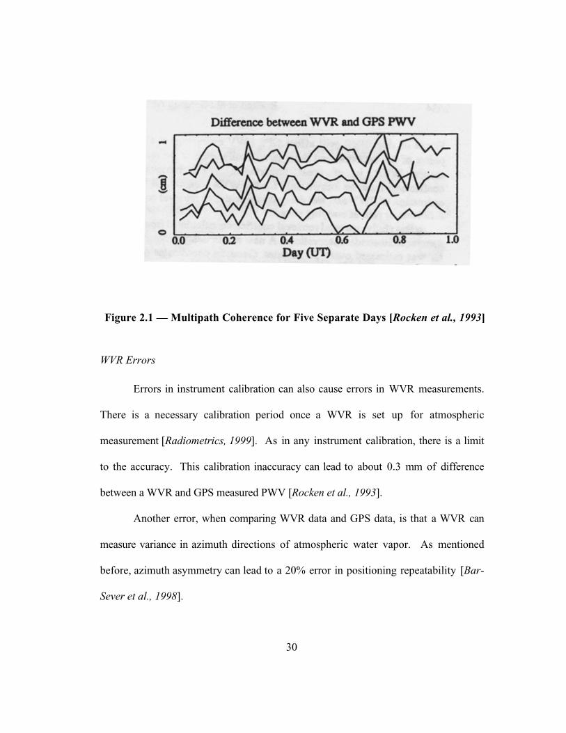
primary source for this error. Figure 2.1 contains PWV time series for five separate

days of data. Please note that data from each day are arbitrarily offset from one

another. For the UNAVCO experiment, about 1 mm of error was attributed to

multipath.

30

Figure 2.1 — Multipath Coherence for Five Separate Days [Rocken et al., 1993]

WVR Errors

Errors in instrument calibration can also cause errors in WVR measurements.

There is a necessary calibration period once a WVR is set up for atmospheric

measurement [Radiometrics, 1999]. As in any instrument calibration, there is a limit

to the accuracy. This calibration inaccuracy can lead to about 0.3 mm of difference

between a WVR and GPS measured PWV [Rocken et al., 1993].

Another error, when comparing WVR data and GPS data, is that a WVR can

measure variance in azimuth directions of atmospheric water vapor. As mentioned

before, azimuth asymmetry can lead to a 20% error in positioning repeatability [Bar-

Sever et al., 1998].

31

Pressure Sensor Errors

Pressure sensor errors affect the calculation of the hydrostatic delay, εd, in

Equation 2.6. As with any measurement device, there are very small errors in

calibration. For an error of 1 mbar, the error in PWV can be about 0.5 mm [Rocken et

al., 1993].

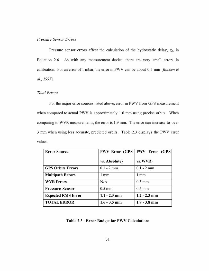
Total Errors

For the major error sources listed above, error in PWV from GPS measurement

when compared to actual PWV is approximately 1.6 mm using precise orbits. When

comparing to WVR measurements, the error is 1.9 mm. The error can increase to over

3 mm when using less accurate, predicted orbits. Table 2.3 displays the PWV error

values.

Error Source PWV Error (GPS

vs. Absolute)

PWV Error (GPS

vs. WVR)

GPS Orbits Errors 0.1 - 2 mm 0.1 - 2 mm

Multipath Errors 1 mm 1 mm

WVR Errors N/A 0.3 mm

Pressure Sensor 0.5 mm 0.5 mm

Expected RMS Error 1.1 - 2.3 mm 1.2 - 2.3 mm

TOTAL ERROR 1.6 - 3.5 mm 1.9 - 3.8 mm

Table 2.3 - Error Budget for PWV Calculations

32

Chapter 3 — The GPS Network and Computational Procedure

The GPS Network

The Continuously Operating Reference Stations (CORS) network gathers data

from 16 GPS receivers in Texas and its surrounding states for near real time PWV

processing. For this project, four additional receivers specifically were placed

strategically to fill in geographical gaps left by the CORS receivers. Because an

Internet connection for data upload was needed at each receiver location, colleges and

universities were ideal choices for these GPS sites. There is no CORS antenna located

near Austin, Texas, with data available hourly (data from the CORS site, AUS5, is

only published once a day), so a GPS antenna was placed on the roof of the building

in which CSR is located. The other permanent GPS sites were installed at universities

in Wichita Falls, Brownwood, and Laredo, Texas. More detail will be presented in the

next section regarding the specifics of the site installations. Table 3.1 shows a

complete list of GPS sites used for near real time PWV processing, and the agency

responsible for their maintenance and upkeep. Figure 3.1 shows a map displaying the

location of each receiver used for the experiment.

33

Site Location Lat. Long. Responsible Agency

ARP3 Aransas Pass, Texas 27.8° 262.9° U.S. Coast Guard

AZCN Aztec, New Mexico 36.8° 252.1° Forecast Systems Lab

BRWD Brownwood, Texas 31.7° 261.0° Center for Space Research

CSR1 Austin, Texas 30.4° 262.3° Center for Space Research

DQUA Dequeen, Arkansas 34.1° 265.7° Forecast Systems Lab

ENG1 English Turn, Louisiana 29.9° 270.1° U.S. Coast Guard

GAL1 Galveston, Texas 29.3° 265.3° U.S. Coast Guard

HKLO Morris, Oklahoma 35.7° 264.1° Forecast Systems Lab

JTNT Jayton, Texas 33.0° 259.0° Forecast Systems Lab

LMNO Lamont, Oklahoma 36.7° 262.5° Forecast Systems Lab

LRDO Laredo, Texas 27.6° 260.6° Center for Space Research

MDO1 Ft. Davis, Texas 30.7° 256.0° International GPS Service

PATT Palestine, Texas 31.8° 264.2° Forecast Systems Lab

PRCO Purcell, Oklahoma 35.0° 262.5° Forecast Systems Lab

SJT2 San Angelo, Texas 31.4° 259.5° FAA/NTSB

TCUN Tucumcari, New Mexico 35.1° 256.4° Forecast Systems Lab

VCIO Vici, Oklahoma 36.1° 260.8° Forecast Systems Lab

WNFL Winnfield, Louisiana 31.9° 267.2° Forecast Systems Lab

WSMN White Sands, New Mexico 32.4° 253.7° Forecast Systems Lab

WTFL Wichita Falls, Texas 33.9° 261.5° Center for Space Research

Table 3.1 - Antenna Site Locations and Responsible Agencies

34

Symbol Legend

CSR

FSL

USCG

IGS

FAA/NTSB

Figure 3.1 - Map of GPS Receiver Locations [Whitlock et al., 1999]

GPS Site Installation

Representatives from Howard Payne University in Brownwood, Texas A&M

International University in Laredo, and Midwestern State University in Wichita Falls

35

agreed to assist the project by hosting GPS equipment at their respective campuses.

For each of these three sites, a Trimble choke ring antenna and Paroscientific MET3

sensor were installed on the roof. Antenna and meteorological sensor cables

connected the antenna to the receiver/PC located in a lab, then the PC was connected

to the Internet for data upload.

Site Requirements

For each potential GPS site location, several criteria must be satisfied to

receive, log, and transfer GPS data. In order to receive good data, the potential GPS

antenna location must have a clear view of the sky. Also, there must not be any

interference in the L-band (1575.4 MHz and 1227.6 MHz for L1 and L2) that would

worsen the signal-to-noise ratio of the GPS signal as received by the antenna. The

GPS receiver and PC must be in a secure environment, with power and Internet

access. Finally, a physical pathway to connect the cable from the antenna and

meteorological sensor on the roof to the receiver in the lab must be established.

Hardware for Each CSR Installed Site

The following were the major hardware items taken and installed at each site:

• 1 Trimble choke ring GPS antenna with spherical raydome and 30 meters of cable

• 1 Trimble 4000SSi receiver with an Office Support Module 2 (OSM2) power unit

• 1 Paroscientific MET3 Sensor with 30 to 60 meters of cable

36

• 1 Linux platform Personal Computer (PC) with monitor

• 1 Uninterrupted Power Supply (UPS)

These hardware items were purchased for the project and installed at the three

selected sites in Brownwood, Wichita Falls, and Laredo. These same items were

installed in Austin at the Center for Space Research facility, except that the cable was

longer (100 m) and needed two signal and DC voltage boosters installed along the

cable. The MET3 cable was also 100 m, and instead of a Linux based PC, a Hewlett

Packard workstation was used. The configuration for the hardware is diagrammed

later, in Figure 3.4.

Antenna Installation

For each antenna installation, a threaded rod was placed in a drilled hole and

fixed with epoxy. A plate (Figure 3.2) to allow for fine leveling of the antenna was

locked onto the threaded rod with thread-locking cement. Once locked onto the plate,

the antenna is leveled and the raydome cover installed to protect the antenna from the

elements (Figure 3.3). The Paroscientific MET3 meteorological sensor was installed

near the antenna, and the antenna and MET3 cables were run together to reach the

receiver and PC in a secure laboratory.

37

Figure 3.2 - Leveling Plate (BRWD)

Figure 3.3 - Complete Antenna with Raydome (BRWD)

38

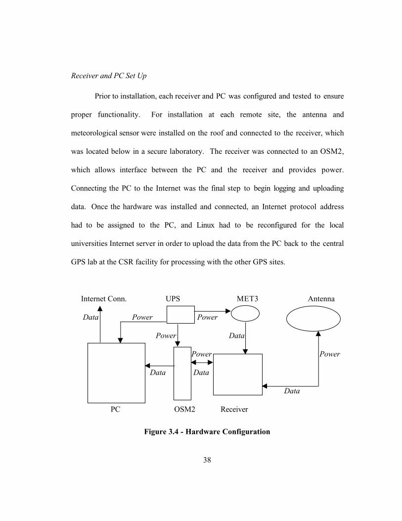
Receiver and PC Set Up

Prior to installation, each receiver and PC was configured and tested to ensure

proper functionality. For installation at each remote site, the antenna and

meteorological sensor were installed on the roof and connected to the receiver, which

was located below in a secure laboratory. The receiver was connected to an OSM2,

which allows interface between the PC and the receiver and provides power.

Connecting the PC to the Internet was the final step to begin logging and uploading

data. Once the hardware was installed and connected, an Internet protocol address

had to be assigned to the PC, and Linux had to be reconfigured for the local

universities Internet server in order to upload the data from the PC back to the central

GPS lab at the CSR facility for processing with the other GPS sites.

Internet Conn. UPS MET3 Antenna

Data Power Power

Power Data

Power Power

Data Data

Data

PC OSM2 Receiver

Figure 3.4 - Hardware Configuration

39

Firmware Configuration

Each Trimble 4000SSi receiver is configured to sample observation data every

15 seconds with a 4° satellite elevation mask. Through the Control Menu via the

MET/TILT Interface , the Repeat String is set for "05 *9900P9N" which samples

the pressure, temperature, and relative humidity automatically every five minutes, and

writes them to the data file. Data files are continuously taken at 60 minute

increments. The data file that is downloaded hourly contains observation,

meteorological, and navigation RINEX data.

Computational Procedure

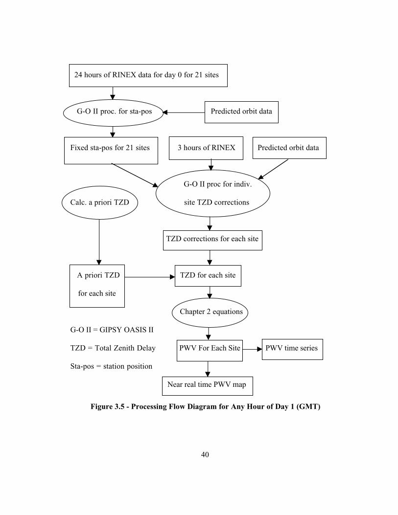
Figure 3.5 summarizes the overall processing procedure. Before the GPS data

is processed for PWV calculations, pre-established positions for the antenna sites

must be estimated. To fix the coordinates of each GPS antenna, the RINEX data for

the entire day for each available GPS site are processed with GIPSY-OASIS from the

Jet Propulsion Laboratory (JPL). This position is then fixed for PWV estimation

purposes for the entire subsequent day. GIPSY-OASIS is also used to process the

near real time GPS data to eventually estimate a tropospheric zenith delay for each

receiver, which are translated into PWV by using the equations in Chapter 2. Time

series for PWV, as well as temperature and pressure, are then produced. For PWV

contour mapping purposes, PWV values are averaged over the hour. This single PWV

value, along with antenna latitude and longitude, is input into Generic Mapping Tools

40

24 hours of RINEX data for day 0 for 21 sites

G-O II proc. for sta-pos Predicted orbit data

Fixed sta-pos for 21 sites 3 hours of RINEX Predicted orbit data

G-O II proc for indiv.

Calc. a priori TZD site TZD corrections

TZD corrections for each site

A priori TZD TZD for each site

for each site

Chapter 2 equations

G-O II = GIPSY OASIS II

TZD = Total Zenith Delay PWV For Each Site PWV time series

Sta-pos = station position

Near real time PWV map

Figure 3.5 - Processing Flow Diagram for Any Hour of Day 1 (GMT)

41

software, which produces a detailed map of PWV over Texas and its surrounding

states [Wessel and Smith, 2000]. These maps and time series are then placed on the

Internet in near real time for the public to use.

Downloading GPS Data

GPS RINEX data are gathered from the CORS network at

ftp://cors.ngs.noaa.gov/cors/rinex

The Trimble receivers installed by the Center for Space Research upload their data

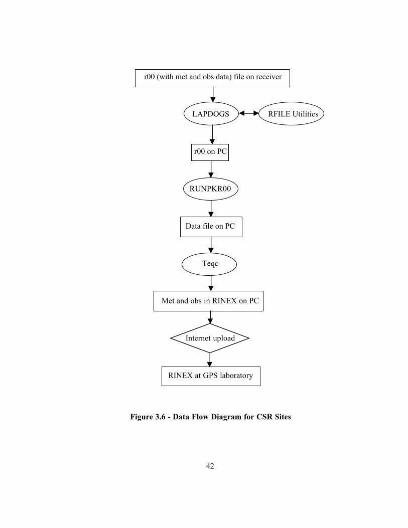
every hour (on the hour) to personal computers at each specific site. Figure 3.6

outlines the data gathering and processing algorithm performed hourly to quality

check and convert the raw data to RINEX format for each CSR installed site. Local

Automated Process for Downloading of Global Sites (LAPDOGS) software, from

UNAVCO, is used to take the raw data from the Trimble 4000 SSi receiver and place

it on the hard drive of the computer. Rfile Utilities software, a series of executable

files acquired from Trimble, is needed to run the LAPDOGS program. The

downloaded data is in r00 format (filename.r00) and must be converted using

runpkr00 (one of the executable files in the Rfile utilities) to data file format

(filename.dat, filename.eph, filename.mes, filename.ion). Next, teqc, also distributed

by UNAVCO, performs a quality check on the data, and converts it to the RINEX

format that is ASCII readable and the data format input to GIPSY-OASIS. Both

meteorological and observation data are converted to RINEX using this procedure.

42

r00 (with met and obs data) file on receiver

LAPDOGS RFILE Utilities

r00 on PC

RUNPKR00

Data file on PC

Teqc

Met and obs in RINEX on PC

Internet upload

RINEX at GPS laboratory

Figure 3.6 - Data Flow Diagram for CSR Sites

43

Finally, the observation and meteorological RINEX files are uploaded to a computer

in the GPS lab at the Center for Space Research for combined processing.

Daily Station Position Runs

Once data for an entire day is available, GIPSY-OASIS takes the site position

and velocity from CORS site log files as a priori, then estimates a new station

position. This position is used for initializing the scheme for the daily PWV

estimation. Initial experimentation showed that fixing the position in this manner gave

more stable PWV estimates, especially when compared to independently determined

PWV data [Gabor, 1997].

Estimation Background

Observations, z, are modeled as a function of parameters, x, as [Gregorius,

1996]

z = F(x) + Data Noise + Mismodeling (3.1)

where F(x) must be linearized using Taylor expansion to

z F x F x F x x x O x= ≈ + − +( ) ( ) ' ( )( ) ( )0 0 0 0 (3.2)

or

δ δz A x= (3.3)

where δz = z - F(x0), A = F’(x0), and δx = (x - x0). x0 are the nominal values of the

model parameters and A is their matrix of change. GIPSY-OASIS tries to find the best

44

solution to Equation 3.3, which is the best least squares agreement between the model

and observations. Next, we introduce pre-fit residuals, v, to Equation 3.3 (and drop

the δ’s for convenience) to get

z Ax v= + (3.4)

where z now represents the observed minus the computed values, A is the partial

derivative matrix of parameters, or design matrix, and then solve for x. This set of

equations yields one equation per observation. We define the parameter covariance

matrix as

P A WAxT

ˆ ( )= −1(3.5)

where W is the a priori weight matrix of the observations and is the inverse of the

covariance of observational errors. The values in W cannot be computer

mathematically, but instead from previous experience. The weighted least squares of

residuals is then

ˆ ˆ min.v WvT = (3.6)

The estimate of the corrections to the initial values assumed for the parameters is then

ˆ ˆx P tx= (3.7)

where

t A WzT= (3.8)

from the normal equations, giving the final solution

x x P t x A WA A WzxT T*

ˆ ( )= + = + −0 0

1(3.9)

45

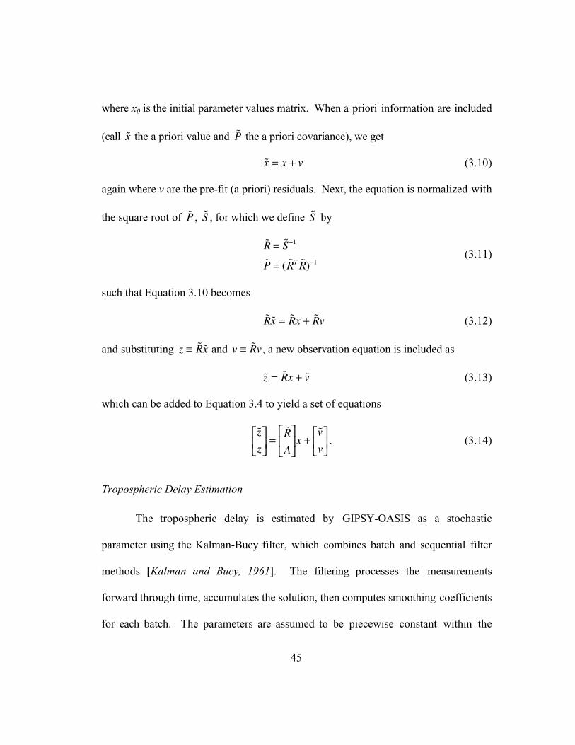
where x0 is the initial parameter values matrix. When a priori information are included

(call x̃ the a priori value and P̃ the a priori covariance), we get

x̃ x v= + (3.10)

again where v are the pre-fit (a priori) residuals. Next, the equation is normalized with

the square root of P̃ , S̃ , for which we define S̃ by

˜ ˜

˜ ( ˜ ˜ )

R S

P R RT

=

=

−

−

1

1(3.11)

such that Equation 3.10 becomes

˜ ˜ ˜ ˜Rx Rx Rv= + (3.12)

and substituting z Rx≡ ˜ ˜ and v Rv≡ ˜ , a new observation equation is included as

˜ ˜ ˜z Rx v= + (3.13)

which can be added to Equation 3.4 to yield a set of equations

˜ ˜ ˜z

z

R

Ax

v

v

=

+

. (3.14)

Tropospheric Delay Estimation

The tropospheric delay is estimated by GIPSY-OASIS as a stochastic

parameter using the Kalman-Bucy filter, which combines batch and sequential filter

methods [Kalman and Bucy, 1961]. The filtering processes the measurements

forward through time, accumulates the solution, then computes smoothing coefficients

for each batch. The parameters are assumed to be piecewise constant within the

46

batch, then the time is updated and a new batch is processed. The user can input the

length of the batches for estimation. For this processing of PWV, data were

processed in 600 second batches, meaning a value for zenith delay was estimated

every 600 seconds. The sequential filter used is a numerically stable and

computationally fast Square Root Information Filter, which is needed for the quantity

of data processed in the near real time PWV calculations [Gregorius, 1996].

The dynamic system is linearized by Taylor expansion and the parameters in

GIPSY-OASIS are split into three categories: satellite states, stochastic parameters,

and constant bias parameters.

The state vector, X, (x from above) is defined as [GIPSY, 1999]

X

x

x

x

sat

sto

bia

=

(3.15)

where rxsat contains the state of the satellite,

rxsto contains the stochastic parameters

(including tropospheric delay) to be estimated, and the vector rxbia contains the

constant bias parameters that corrupt the satellite state. rX includes the individual

state and process noise vectors and the common parameters between satellites, such

as station coordinates. The linearized state propagation (from time tk-1 to tk) and

observation state equations, with process noise added is the system can be

represented by [GIPSY, 1999; Gregorius, 1996].

47

x t

x t

x t

t t t t t t

t t

I

x t

x t

x t

sat k

sto k

bia k

satd

k k sats

k k satb

k k

sto k k

sat k

sto k

bia k

( )( )( )

=( ) ( ) ( )

( )

( )( )( )

− − −

−

−

−

−

Φ Φ ΦΦ

, , ,

,1 1 1

1

1

1

1

0 0

0 0

+ ( )

−

0

01w tk (3.16)

where Φdsat(tk,tk-1) is the deterministic portion of the satellite-state update, Φs

sat

(tk,tk-1) is the stochastic portion of the satellite-state update, Φbsat(tk,tk-1) is the

constant bias parameter portion of the satellite-state update, Φsto(tk,tk-1) is the

stochastic parameters transition matrix, and I is the identity matrix, as the bias

parameters are constants. w(tk-1) is a Gauss-Markov random walk noise vector with

zero mean.

The GPS data are processed to estimate the stochastic parameter of correction

to an initial guess of zenith tropospheric delay. The a priori guess for zenith

tropospheric delay has both a wet component and hydrostatic component. The

hydrostatic guess is [GIPSY, 1999]

2 2927 0 000116. * . *e h− meters (3.17)

which is dependent solely upon the station height above the geoid, as higher elevation

sites have less atmosphere through which the signal travels (meaning less hydrostatic

delay). The wet component guess is 0.10 meters and is a constant. These are just

initial guesses for the GIPSY-OASIS filter and need not be extremely accurate.

For example, the station in Wichita Falls, TX is about 271.48 m above the

geoid. The a priori estimate of dry delay would be 2.228 m based upon Equation

48

3.17, adjusted to 2.328 m to include the wet component guess. The station position

is held fixed while the correction to the a priori (2.328 m) tropospheric delay is then

estimated through time, in 600 second (10 minute) increments.

The clock drift of each receiver clock must also be estimated. To estimate

these drifts, the CORS station in Algonquin Park, Ontario, is included as the reference

clock in the processing as it has a highly accurate hydrogen maser clock. By using a

stable clock, the drift for the other clocks can accurately be estimated.

Post-GIPSY-OASIS Processing

First, the corrections to the initial guess of total zenith atmospheric delay are

combined with the GIPSY-OASIS tropospheric zenith delay output for a corrected

zenith troposphere delay estimate. Once the atmospheric data are gathered, any

meteorological data point and tropospheric zenith delay data point within 100

seconds of one another are considered a sample point. The surface pressure value

from the meteorological data is used to estimate hydrostatic zenith delay, which is

subtracted off of the corrected tropospheric zenith delay. The remaining value is the

wet tropospheric zenith delay. This is converted to zenith PWV using Equation 2.14.

See Appendix A for a sample calculation of PWV using pressure, temperature, and

zenith delay. Several PWV values are gathered over each hour of interest and the

PWV values are averaged over the hour to obtain a single value to include on the

contour map. All PWV values that are estimated are included in the time series

49

graphs. The hourly value of zenith PWV for each site is input into the GMT

software package and a map in JPEG format is produced detailing water vapor over

the Texas region. Then, the PWV, surface pressure, and surface temperature are

graphed in time series using MATLAB for placement on the Internet.

50

Chapter 4 - Water Vapor Results

Automated computer routines were implemented to process all the available

GPS sites once an hour, every hour of every day. For the purpose of data processing

in this project, Greenwich Mean Time (GMT) is the time standard used. This

eliminates any problems with time zone differences and daylight savings time and is

also the method that the GPS networks reference their data with regard to day of year

and GPS week. RINEX data from the non-CSR GPS sites are available in hour long

files about 30 - 40 minutes after the hour. Once the data files are posted, the

automatic script gathers all of the available meteorological and observation data. Any

time the observation data are available, the site is included for processing regardless of

the availability of the meteorological data. Predicted orbits for the GPS satellites are

downloaded, then the data from the most recent three hours are processed. The

GIPSY-OASIS filter seemed most stable when more than one hour was processed, but

the data to be processed were limited to three hours to save computation time. Once

GIPSY-OASIS has completed processing the data, the output from the most recent

hour is converted from zenith delay to PWV. A time series of 24 hours of PWV for

each site is constructed by taking 23 hours of previously converted PWV and adding

the PWV data from the most recent hour to the end. A near real time PWV map and

individual site 24 hour time series graphs are placed on the Internet at:

http://www.csr.utexas.edu/texas_pwv/real_time/total.html

51

In addition to showing how near real time PWV measurement could be done

with GPS, some selected data were post-processed to determine the accuracy of

predicted orbits in the near real time application. A comparison of GPS orbit

accuracy was done for February 26, 2000 in order to see how the PWV results are

affected by predicted orbit inaccuracies.

Near Real Time Results

The contour maps and PWV time series are produced quickly and accurately.

The data are automatically processed hourly, and accurate PWV estimations within

one hour are produced with no human interaction required.

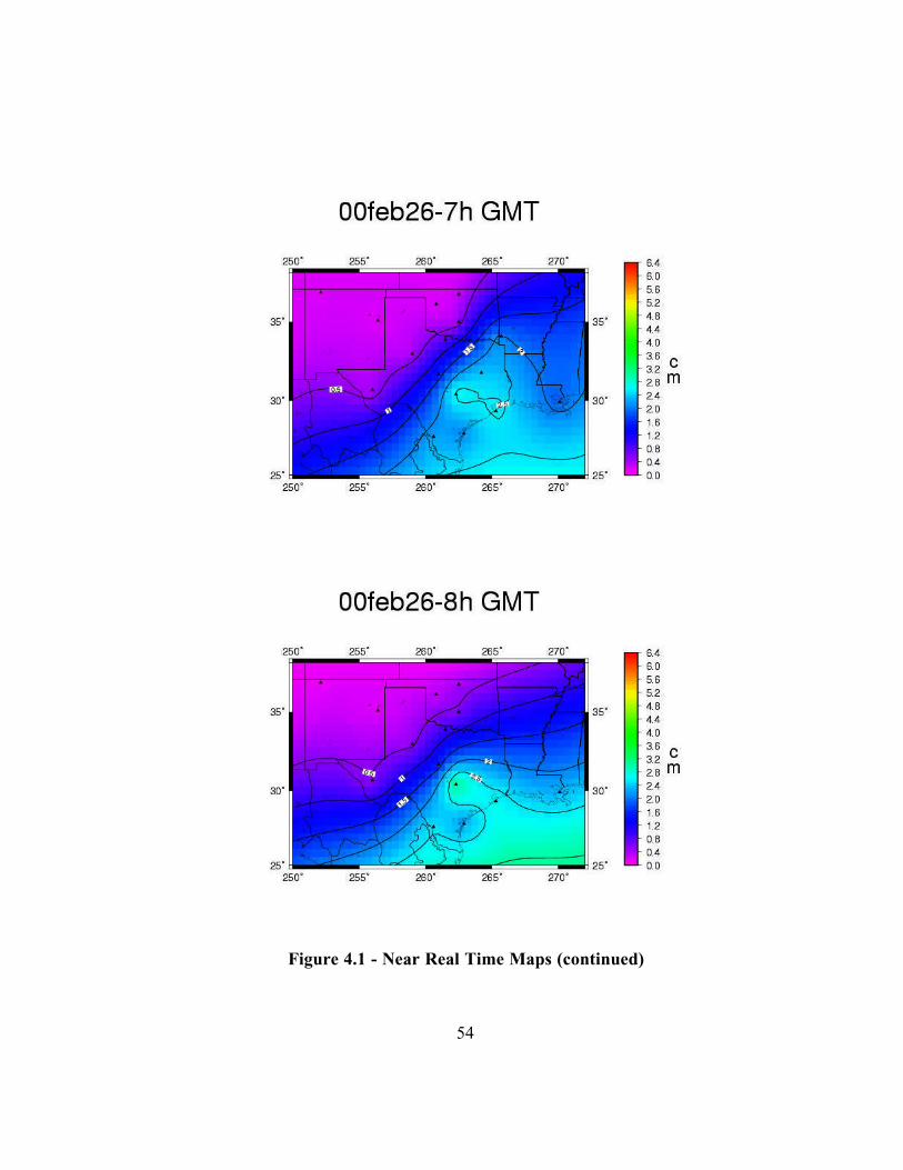
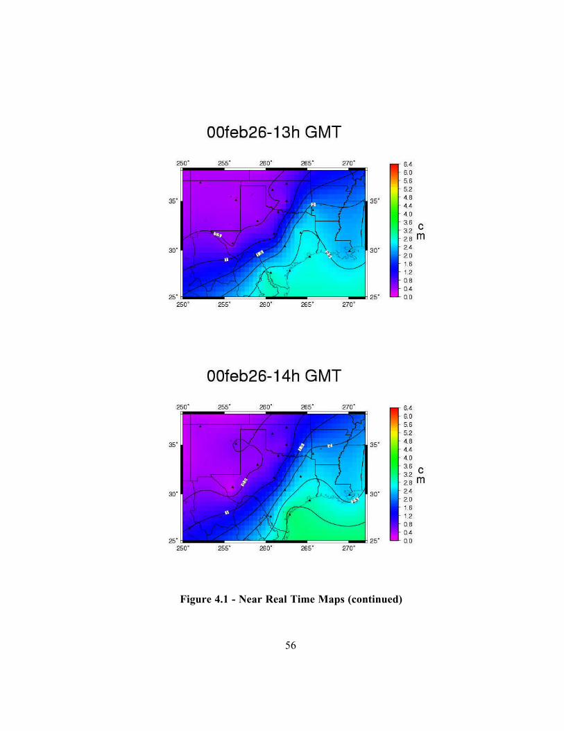
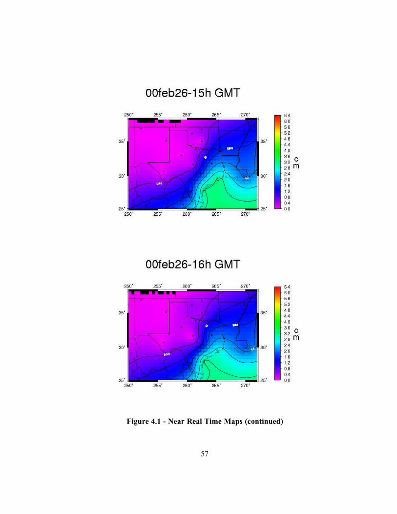
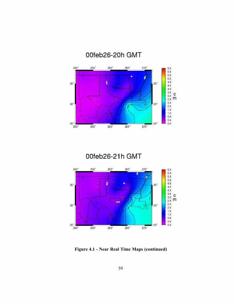
Time Series of Maps

Figure 4.1 is several hourly PWV maps for February 26, 2000. The data from

this day is interesting because it can be seen how rapidly water vapor can change in

time. February 26, 2000, began relatively moist but as a slight cold front pushed

through the Texas region, noticeably dryer air was present by the end of the day. A

significant drop in temperature (up to 9° C) was seen by the GPS sites that

experienced the most significant PWV decrease (Figure 4.2). For these maps and time

series presented here, predicted orbit files were used. Later in the chapter, the result

of changing the type of orbit used will be discussed.

52

Figure 4.1 - Near Real Time Maps

53

Figure 4.1 - Near Real Time Maps (continued)

54

Figure 4.1 - Near Real Time Maps (continued)

55

Figure 4.1 - Near Real Time Maps (continued)

56

Figure 4.1 - Near Real Time Maps (continued)

57

Figure 4.1 - Near Real Time Maps (continued)

58

Figure 4.1 - Near Real Time Maps (continued)

59

Figure 4.1 - Near Real Time Maps (continued)

60

The hour listed in each map title is the beginning of the hour that the map

represents. For instance, if the hour is 0h GMT, this indicates that the data were

averaged over 12:00 a.m. - 1:00 a.m. GMT, or the 0th

hour that day. Similarly for 2h

GMT, the data is for 2:00 a.m. - 3:00 a.m. A 24 hour system is used, so 14h

translates to 2:00 p.m. - 3:00 p.m. GMT. This day contains data for every site

except WSMN and HKLO. SJT2 is included occasionally on the maps, but the

availability of meteorological data is not reliable for that site. The stations in central

and south central Texas (BRWD, CSR1, PATT, JTNT, and ARP3), experience a drop

of 2 - 3 cm of PWV throughout the day.

Time Series of PWV, Temperature, and Pressure

Figure 4.2 shows PWV, pressure, and temperature time series for four

individual sites on the same day. These are the time series that are produced for

public use on the Internet. Pressure and temperature data are taken directly from the

RINEX meteorological data available from each station, while the PWV was estimated

using the algorithm and equations in Chapters 2 and 3. Time is displayed in decimal

day of year, so 57.5 is noon (GMT) on day 57 (February 26, 2000).

61

57 57.1 57.2 57.3 57.4 57.5 57.6 57.7 57.8 57.9

0.5

1

1.5

2

2.5

3

3.5

PWV for arp3

DOY in GMT

PW

V -

in c

m

57 57.1 57.2 57.3 57.4 57.5 57.6 57.7 57.8 57.9

1009

1010

1011

1012

1013

1014

1015

1016

1017

1018

1019

Surface Pressure for arp3

Pre

ssur

e in

mba

r

57 57.1 57.2 57.3 57.4 57.5 57.6 57.7 57.8 57.9

16

18

20

22

24

26

28

Temperature for arp3

DOY in GMT

Tem

pera

ture

in d

egre

es C

Figure 4.2 - Day 2/26/00 Time Series (ARP3)

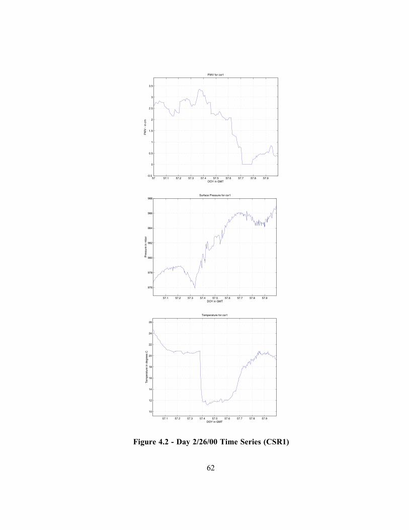
62

57 57.1 57.2 57.3 57.4 57.5 57.6 57.7 57.8 57.9-0.5

0

0.5

1

1.5

2

2.5

3

3.5

PWV for csr1

DOY in GMT

PW

V -

in c

m

57.1 57.2 57.3 57.4 57.5 57.6 57.7 57.8 57.9

976

978

980

982

984

986

988Surface Pressure for csr1

DOY in GMT

Pre

ssur

e in

mba

r

57.1 57.2 57.3 57.4 57.5 57.6 57.7 57.8 57.9

10

12

14

16

18

20

22

24

26

Temperature for csr1

DOY in GMT

Tem

pera

ture

in d

egre

es C

Figure 4.2 - Day 2/26/00 Time Series (CSR1)

63

57 57.1 57.2 57.3 57.4 57.5 57.6 57.7 57.8 57.9

0

0.5

1

1.5

2

2.5

3

3.5

4

PWV for patt

DOY in GMT

PW

V -

in c

m

57 57.1 57.2 57.3 57.4 57.5 57.6 57.7 57.8 57.9

996

997

998

999

1000

1001

1002

1003

1004

1005

Surface Pressure for patt

DOY in GMT

Pre

ssur

e in

mba

r

57 57.1 57.2 57.3 57.4 57.5 57.6 57.7 57.8 57.9

12

14

16

18

20

22

24

Temperature for patt

DOY in GMT

Tem

pera

ture

in d

egre

es C

Figure 4.2 - Day 2/26/00 Time Series (PATT)

64

57 57.1 57.2 57.3 57.4 57.5 57.6 57.7 57.8 57.9-0.5

0

0.5

1

1.5

2

PWV for wtfl

DOY in GMT

PW

V -

in c

m

57.1 57.2 57.3 57.4 57.5 57.6 57.7 57.8 57.9

972

974

976

978

980

982

984Surface Pressure for wtfl

DOY in GMT

Pre

ssur

e in

mba

r

57.1 57.2 57.3 57.4 57.5 57.6 57.7 57.8 57.9

6

8

10

12

14

16

18

20

22

Temperature for wtfl

DOY in GMT

Tem

pera

ture

in d

egre

es C

Figure 4.2 - Day 2/26/00 Time Series (WTFL)

65

Discussion of Near Real Time Results

The small cold front that reduced PWV noticeably throughout the region

moved from the northwest to the southeast on February 26, 2000. PATT and CSR1

saw the most significant temperature and PWV drops. PWV dropped from above 3

cm to near 0 cm over an eight hour period for both sites. The temperature at CSR1

went from 21° C to 12° C in less than an hour (at about 1:00 a.m. Central Standard

Time). A peak value of 3.3 cm of PWV was estimated at the same time as the

temperature drop began, meaning much dryer air in the troposphere was following the

front. PATT saw a decrease in temperature from 21° C to 12.5° C at nearly the same

time as the temperature drop at CSR1. PATT saw a peak value of 3.6 cm PWV at the

same time as the temperature drop began. ARP3, located much further south,

experienced a smaller temperature decrease from 25° C to 18° C about six hours after

the CSR1 and PATT temperature drop. The front had already past WTFL at the

beginning of the day, as no distinct temperature drop was observed. However, the

temperature did not reach the same high at the end of day 57 (16.5° C) as the

beginning of the day (21° C), which is an indication that the cold front had passed

through. The pressure profiles look similar for each of the four sites, with noticeable

pressure increases throughout the day.

66

Effect of Orbit Accuracy on PWV

Three types of orbit files were compared to better understand how the

prediction of satellite orbits affects near real time PWV errors. For comparison, the

precise orbits were used to compare with two levels of predicted orbits. JPL orbits

were chosen as the only orbits for all experimentation because GIPSY-OASIS is JPL

software and the quality of the orbits are highly regarded.

Orbit and Polar Motion Data

For near real time processing, it is desirable to gather the most accurate

predicted GPS orbit and polar motion data available. GIPSY-OASIS requires two

files, YEAR-MO-DY.eci.predict.edited and YEAR-MO-DY.tpeo.predict, where YEAR is

the four digit year (i.e. 1999 or 2000), MO is the two digit month (01-12) and DY is

the two digit day of month (01-31). The first file is a GPS satellite orbit data file (in

.eci format) and the other is an Earth and polar motion data file (in tpeo.nml format)

which is needed to establish the geodetic reference frame. These files are available at:

ftp://sideshow.jpl.nasa.gov/pub/gipsy_products/caveat_emptor/orbits

and are typically updated daily, with each file containing satellite orbit data for the

day in the filename and up to three days before or after. Therefore, 1999-05-

10.eci.predict.edited could be used to evaluate any day between May 7th

and May

13th

. Every hour the automated script looks for the latest of these files for use in

GIPSY-OASIS processing. Once the latest possible day is found, the script will no

67

longer look for a later version (saving computation time and workload) until a new day

is started. The latest possible orbit files are from the day before; for instance

sometime on May 11th

, 1999, the file 1999-05-10.eci.predict.edited will be posted.

For the purpose of discussion here, the date in the title will be labeled the date of the

predicted orbit files. "One day predicted orbits" means that the date in the orbit file

name is one day before the day being processed. "Two day predicted orbits" means

that the date in the orbit file name is two days before the day being processed, and

therefore is expected to be slightly less accurate than the one day predicted orbits.

Sometimes it is necessary to use predicted orbit files that are three days old, but this

was a rare occurrence and will not be implemented for comparison here. For orbit

accuracy comparison, the RINEX data will also be processed using precise orbits,

generally available two weeks after a given date.

Orbit Comparison Results

Figure 4.3 displays the PWV time series graphs of several sites for February

26, 2000. In each case, the three different kinds of orbits are plotted together for

comparison. Figure 4.3 shows how the PWV data differs for ARP3, CSR1, MDO1,

TCUN, and WTFL with respect to orbit accuracy, but not from any independently

measured value.

68

57 57.1 57.2 57.3 57.4 57.5 57.6 57.7 57.8 57.9

0.5

1

1.5

2

2.5

3

3.5

PWV for arp3

DOY in GMT

PW

V i

n cm

57 57.1 57.2 57.3 57.4 57.5 57.6 57.7 57.8 57.90.5

0

0.5

1

1.5

2

2.5

3

3.5

PWV for csr1

DOY in GMT

PW

V i

n cm

------------------------------------------ Precise orbits

+ + + + + + + + + + + + + + + + + One day predicted orbits

. . . . . . . . . . . . . . . . . . . . . . . . . . . . . Two day predicted orbits

Figure 4.3 - Orbit Comparison for Five Sites - 2/26/00

69

57 57.1 57.2 57.3 57.4 57.5 57.6 57.7 57.8 57.90.2

0

0.2

0.4

0.6

0.8

PWV for mdo1

DOY in GMT

PW

V i

n cm

57 57.1 57.2 57.3 57.4 57.5 57.6 57.7 57.8 57.90.2

0.1

0

0.1

0.2

0.3

0.4

0.5

0.6

0.7

0.8

PWV for tcun

DOY in GMT

PW

V i

n cm

------------------------------------------ Precise orbits

+ + + + + + + + + + + + + + + + + One day predicted orbits

. . . . . . . . . . . . . . . . . . . . . . . . . . . . . Two day predicted orbits

Figure 4.3 - Orbit Comparison for Five Sites - 2/26/00 (continued)

70

57 57.1 57.2 57.3 57.4 57.5 57.6 57.7 57.8 57.90.2

0

0.2

0.4

0.6

0.8

1

1.2

1.4

1.6

PWV for wtfl

DOY in GMT

PW

V i

n cm

------------------------------------------ Precise orbits

+ + + + + + + + + + + + + + + + + One day predicted orbits

. . . . . . . . . . . . . . . . . . . . . . . . . . . . . Two day predicted orbits

Figure 4.3 - Orbit Comparison for Five Sites - 2/26/00 (continued)

Orbit Data Comparison

Table 4.1 gives a data comparison for the PWV values estimated for the five

sites that are graphed in time series above. The PWV results from using one day

predicted orbits and two day predicted orbits are compared independently to the

precise orbit case, and a residual for each time epoch is calculated and averaged in an

rms sense. A maximum residual is found each day for each site, by comparing the

individual PWV values at each time epoch. The rms values in Table 4.1 were

calculated by squaring the difference in PWV from the predicted orbits and the precise

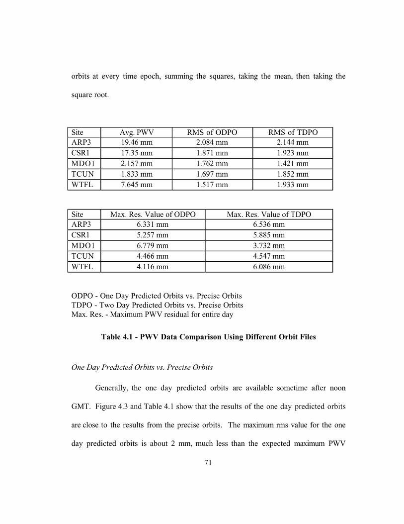
71

orbits at every time epoch, summing the squares, taking the mean, then taking the

square root.

Site Avg. PWV RMS of ODPO RMS of TDPO

ARP3 19.46 mm 2.084 mm 2.144 mm

CSR1 17.35 mm 1.871 mm 1.923 mm

MDO1 2.157 mm 1.762 mm 1.421 mm

TCUN 1.833 mm 1.697 mm 1.852 mm

WTFL 7.645 mm 1.517 mm 1.933 mm

Site Max. Res. Value of ODPO Max. Res. Value of TDPO

ARP3 6.331 mm 6.536 mm

CSR1 5.257 mm 5.885 mm

MDO1 6.779 mm 3.732 mm

TCUN 4.466 mm 4.547 mm

WTFL 4.116 mm 6.086 mm

ODPO - One Day Predicted Orbits vs. Precise Orbits

TDPO - Two Day Predicted Orbits vs. Precise Orbits

Max. Res. - Maximum PWV residual for entire day

Table 4.1 - PWV Data Comparison Using Different Orbit Files

One Day Predicted Orbits vs. Precise Orbits

Generally, the one day predicted orbits are available sometime after noon

GMT. Figure 4.3 and Table 4.1 show that the results of the one day predicted orbits

are close to the results from the precise orbits. The maximum rms value for the one

day predicted orbits is about 2 mm, much less than the expected maximum PWV

72

measurement error of about 3.5 mm and on the order of the expected rms error of 2.3

mm (Table 2.3). The maximum residual is 6.7 mm PWV (MDO1). This error

occurred toward the end of the day (visible in Figure 4.3), and it seems that the one

day predicted orbits estimated two erroneously high PWV values. It should also be

noted that the graphs for TCUN and MDO1 appear at first glance to display PWV

values that do not follow the precise orbits closely, but because the PWV is very low

at these sites, the scale on the graph is much finer than the scale for the other four

sites. Those two sites exhibit two of the smallest three rms of residuals for the day.

The maximum residual for the one day predicted orbit case varies between 4.1 and 6.7

mm for the five chosen sites.

Two Day Predicted Orbits vs. Precise Orbits

Before the one day predicted orbits are made available, the two day predicted

orbits are used for near real time processing. The maximum PWV rms values for these

five sites was 2.1 mm, almost identical to the one day predicted orbit case. The rms

values were slightly higher for 4 of the 5 sites, while MDO1 showed a slightly lower

rms for the two day predicted orbit case (most likely due to the seemingly erroneous

PWV values toward the end of the day for the one day predicted orbit case). The rms

values are still below the expected PWV accuracy. The maximum residuals for the

two day predicted orbits were near identical to the one day predicted orbit case. The

maximum residuals for these five sites using two day predicted orbit files are actually

73

below the worst case for the one day predicted orbits. The maximum residuals for the

five sites vary between 3.7 mm and 6.5 mm.

Discussion of Orbit Comparison Results

The PWV from one day predicted orbits tend to agree with PWV values found

from precise orbits slightly better than two day predicted orbits, but the difference is

less than 0.5 mm rms. It is desirable that the difference be small, because the two day

predicted orbits must be used until the one day predicted orbits are available. The

near real time estimated PWV shows more oscillation and discontinuity than the

precise orbit calculation because the near real time only processes three hours of data

at a time, while the precise orbits estimated PWV is done by processing all 24 hours

of the day at once. By processing the whole day, the daily time series of total zenith

delay (and subsequently PWV) can be smoothed. The comparison discussed here is

only a comparison of the accuracy of the different orbits, not a comparison of the true

PWV accuracy.

Comparison to Radiosonde measured PWV

Data were obtained from the Department of Energy, Atmospheric Radiation

Measurement (ARM) network [ARM, 2000] which contain PWV measurements made

with radiosonde balloons near the four GPS sites in Oklahoma (the only sites in the

network with regular radiosonde data) for comparison to the near real time PWV

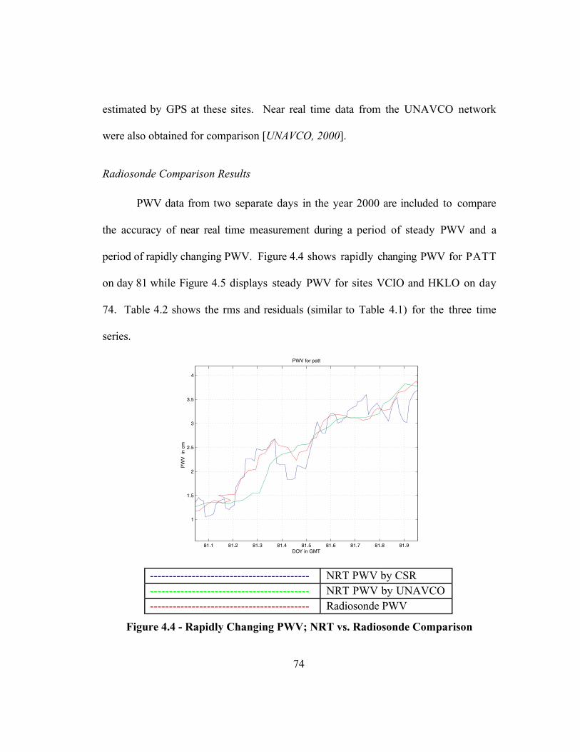
74

estimated by GPS at these sites. Near real time data from the UNAVCO network

were also obtained for comparison [UNAVCO, 2000].

Radiosonde Comparison Results

PWV data from two separate days in the year 2000 are included to compare

the accuracy of near real time measurement during a period of steady PWV and a

period of rapidly changing PWV. Figure 4.4 shows rapidly changing PWV for PATT

on day 81 while Figure 4.5 displays steady PWV for sites VCIO and HKLO on day

74. Table 4.2 shows the rms and residuals (similar to Table 4.1) for the three time

series.

81.1 81.2 81.3 81.4 81.5 81.6 81.7 81.8 81.9

1

1.5

2

2.5

3

3.5

4

PWV for patt

DOY in GMT

PW

V i

n cm

------------------------------------------ NRT PWV by CSR

------------------------------------------ NRT PWV by UNAVCO

------------------------------------------ Radiosonde PWV

Figure 4.4 - Rapidly Changing PWV; NRT vs. Radiosonde Comparison

75

74 74.1 74.2 74.3 74.4 74.5 74.6 74.7 74.8 74.90.6

0.8

1

1.2

1.4

1.6

1.8

2

2.2

2.4

2.6

PWV for vcio

DOY in GMT

PW

V i

n cm

74 74.1 74.2 74.3 74.4 74.5 74.6 74.7 74.8 74.9

0.6

0.8

1

1.2

1.4

1.6

1.8

2

2.2

2.4

2.6

PWV for hklo

DOY in GMT

PW

V i

n cm

------------------------------------------ NRT PWV by CSR

------------------------------------------ NRT PWV by UNAVCO

------------------------------------------ Radiosonde PWV

Figure 4.5 - Steady PWV; NRT vs. Radiosonde Comparison

76

Site Avg. PWV UNAVCO RMS CSR RMS

HKLO 17.44 mm 1.726 mm 2.254 mm

VCIO 15.65 mm 1.576 mm 2.286 mm

PATT 34.64 mm 2.826 mm 2.602 mm

Site UNAVCO Max. Res. Value CSR Max. Res. Value

HKLO 3.227 mm 5.121 mm

VCIO 3.292 mm 4.846 mm

PATT 7.907 mm 6.671 mm

Table 4.2 - UNAVCO and CSR NRT comparison to Radiosonde

Radiosonde Data Comparison

The near real time UNAVCO and CSR estimated PWV are compared

independently to the radiosonde data, and rms of residuals and maximum residual

values are calculated in the same manner as they were when comparing orbit files.

The rms of residuals for near real time PWV estimations are less than 3 mm for

UNAVCO and for CSR. The rms values for the steady PWV case (HKLO and

VCIO) are slightly higher for CSR data compared to UNAVCO data, but are of the

same order of magnitude. The UNAVCO rms is higher for the rapidly changing PWV

case (PATT). The maximum residuals for CSR near real time PWV are higher than

UNAVCO’s by 1.6 - 1.9 mm for the steady PWV case, but much lower for the

rapidly changing PWV case.

77

Discussion of Radiosonde Comparison Results

The rms of residuals between the CSR estimated near real time PWV and

radiosonde data varies from 2.2 mm - 2.6 mm, which is within the allowable error of

3.5 mm and on the order of the expected rms error of 2.3 mm (Table 2.3). The

network and processing algorithms established produce PWV results within the

accuracy expected of independently measured PWV.

During periods of rapidly changing PWV, it is expected that agreement

between independently measured PWV and GPS measured PWV show less agreement

than when PWV values are stable [Nam et al., 1996]. This can be seen in the higher

rms values seen for site PATT for both UNAVCO and CSR measured PWV with

GPS. Figures 4.4 and 4.5 show that the near real time PWV estimations by CSR tend

to oscillate more than the near real time PWV estimations by UNAVCO, yielding

slightly higher maximum residual values. Because the near real time PWV is estimated

in hour segments, it tends to show some slight discontinuities when compared to data

processed in longer segments in which the data is smoothed. However, by not

utilizing smoothing coefficients over longer time periods of data, rapid changes in

PWV over small temporal scales can more accurately estimated, as is seen at time 74.7

for site VCIO in Figure 4.5 or between 81.3 and 81.4 for site PATT in Figure 4.4.

The smoother, UNAVCO solutions to not follow the radiosonde data as well in this

case.

78

Radiosondes have been known to experience problems with their humidity

sensors during periods of rapidly changing weather, which could yield a larger rms for

both UNAVCO and CSR near real time estimated PWV during the rapidly changing

PWV case [Coster et al., 1996; Wade, 1994]

Problems and Delays in Processing

If any step in the entire process is not operating optimally, near real time data

results may not be forthcoming in a timely manner. The following discussion outlines

problems and delays seen repeatedly in the near real time application. These

problems occurred very rarely over the duration of the project, but present issues as

to the feasibility of near real time PWV calculations with GPS.

CORS Downloading

One of the problems in near real time processing is the reliability of the CORS

network posting the RINEX data in near real time. Several times during the 1998,

1999, and 2000 calendar years when data were being processed hourly, CORS data

from one or more sites were not available for unexplained reasons, sometimes for days

at a time. If the data are not available, it obviously cannot be processed. Similarly,

the ftp site from which the data is downloaded occasionally experienced

computational delays. There were times when it could take up to 3 hours just to

download the RINEX data. Generally, this process takes 2 or 3 minutes, so this kind

79

of delay cripples the near real time processing. If the CORS data takes more than a

few minutes to download, the identical delay in the production of output is

experienced.

Orbit Download

Occasionally JPL will delay posting new predicted orbits. Like the CORS

network ftp site, the JPL posted data site can get very slow, sometimes seen in terms

of close to an hour to download the two necessary orbit files. When this delay is

experienced, near real time results are delayed. When operating optimally, it will only

take a few minutes to find the orbit data. Then, once the latest file is found, the script

will not search the JPL server until the next day, eliminating entirely the possibility of

delay. If the orbit files are not present or have not been updated for several days, no

near real time results can be estimated. Because this happens very rarely, no

provision for using broadcast orbits or orbits from another agency was made.

CSR Machine Delays

Because several users at CSR share the computational power of the computer

processor used for near real time PWV processing, delays of significant proportion

can be a result. For instance, if another GIPSY-OASIS routine is running, it can take

up to twice as long for GIPSY-OASIS to process from start to finish. With no other

competing computational workload, hourly processing takes from 10 to 20 minutes.

80

When the CSR computers are filled with several jobs from other users, it can take

from 30 to 65 minutes to complete the processing, causing identical delays in near real

time data results.

Summary of Near Real Time Application

Generally, results from a specific hour are posted on the Internet in less than

one hour after the GPS data collection has ceased. Data file collection begins about 40

minutes after the hour, when CORS posts GPS data files. Then after GIPSY-OASIS

processes for 10 - 20 minutes, the PWV values are estimated and maps and graphs

produced in less than 5 minutes. For example, at 14:00 GMT, data is no longer logged

from the previous hour, 13:00 - 14:00 GMT. At 14:40, the CORS data is ready, then

by 14:55, GIPSY-OASIS is done processing. By 15:00, all the maps and graphs are

done and posted for the time from 13:00 - 14:00. There seems to be little

opportunity to reduce this significantly without access to the data in less than 40

minutes. For instance, data from the four CSR installed sites are available a few

minutes after the hour. If only those sites were to be processed, then processing

could start at 14:05 instead of 14:40.

As a safeguard against repeated crashes of the scripts and overload of

machines, a new hour is only started if GIPSY-OASIS processing from the previous

hour has finished. For instance, if it is taking GIPSY-OASIS 75 minutes to run to

completion (perhaps due to computational workload), most likely the next hour

81

would not be processed. It would only serve to slow down the processing of the

previous hour and output would not be available in a near real time sense anyway. So

during heavy CSR computer use, there are only maps available every two hours,

although this is a rare occurrence as processing usually takes less than 20 minutes.

Catastrophic Errors

Because there are over 20 scripts involved in GIPSY-OASIS processing, there

is a possibility that the processing will fail. To ensure this does not lead to repeated

crashes of the hourly script, many subroutines have been implemented to ensure that

common errors are not fatal. If a routine crashes, the next time the script is run it will

run through properly without human intervention barring any other catastrophic

circumstances. Many times the same error will occur several hours in a row (for

instance if the network at CSR is down and data cannot be written to the directories).

The following are some of the catastrophic errors experienced occasionally during the

near real time processing.

Station Position File Errors

The station position file is the output of the daily processing specifically

designed to estimate station positions. This file is tested to make sure every site has

been included and that GIPSY-OASIS ran through to completion. If both these

criterion are satisfied, the station position file will be updated. If the station position

82

file were updated without station position values for any given station, the hourly

processing cannot be performed. If at least one of the sites is not posting observation

data for an entire day, the entire station position file will not update. Sometimes it

will not update for a few successive days, but this has proven to be enough for

accurate water vapor estimation. Human interaction is required if GIPSY-OASIS runs

all the way through and there were a full compliment of sites, but somehow it does

not run accurately (perhaps because the orbits are not accurate, or one of the RINEX

files has inaccurate data). In this case, the new station position file will be inaccurate

and produce catastrophic results when used the next day in GIPSY-OASIS. Several

old station position files are kept on hand, and the latest, best file must replace the

inaccurate one. Each station position file was arbitrarily set to be accurate for 45

days. If a site is down longer than this, or if at no point during a 45-day period are all

sites present, the station position file will not update and the GIPSY-OASIS

processing will not work with this old file. A new one must be constructed in order

for the near real time processing to continue.

Orbit Errors

Sometimes inaccurate values will be estimated by GIPSY-OASIS due to orbit

file inaccuracy. For instance, an hourly run at 13:00 GMT may run fine, but the run

at 14:00 GMT may show residuals ten times larger, and during each subsequent

hourly run, GIPSY-OASIS may crash altogether. This is generally a sign that the

83

orbit files are inaccurate after a certain time in the orbit file. One reason this might

occur is because of satellite maneuvers, the timing of which are unpredictable [Rocken

et al., 1997]. There is no corrective action to take for this case. Attempts at using

older predicted orbit files have never fixed the problem. Once JPL produces new

predicted orbit files, near real time processing can continue. Of course during the time

the orbit files are inaccurate, no meaningful PWV data can be estimated. This problem

occurs rarely, and typically will become fixed within a few hours.

Computation Load and Network Errors

Occasionally when the CSR machines are overloaded with processing jobs,

GIPSY-OASIS will run into memory problems and fail before completion. Whenever

this was experienced, it seemed to happen several hours in a row. Generally, the

problem would correct itself once the computational load of the computer was

reduced, but a human corrective action would be to change the machine that GIPSY-

OASIS was being processed on, and therefore circumvent the problem. There is no

provision to reprocess the failed run, as the subsequent hourly run will always begin

in less than one hour.

Occasionally, the network that keeps the GPS data, JPL orbits, and GIPSY-

OASIS will be shut down for upgrades or to debug a problem. When this happens,

processing cannot be done. Once the network is back on line, the hourly processing

will continue, however hourly runs that would have occurred will not be redone.

84

Chapter 5 - Conclusions

Accuracy and Weather Modeling

For weather modeling and climate monitoring, it is important to establish the

capability to measure PWV in near real time at an affordable cost [Bevis et al., 1996;

Bevis et al., 1993; Bevis et al., 1992; Coster et al., 1996; Rocken et al., 1993; Yuan et

al., 1993]. Because there is an increasing abundance of GPS data available to the

public, demonstrating PWV estimation capability by using GPS measurements could

be instrumental in establishing this capability. The network of 20 receivers utilized

for this experiment has shown that the Global Positioning System is an accurate and

efficient method for measuring precipitable water vapor. This network has

demonstrated that PWV estimated in near real time with GPS has accuracy of less

than 2.6 mm rms when compared to radiosonde measurements or post-processed GPS

(using precise orbits) PWV estimation. Any network of 12 - 20 GPS receivers over a

relatively small region (such as Texas and its surrounding states) can produce accurate

maps of PWV in near real time (on the order of twenty minutes to an hour after the

processing begins). The addition of more GPS antennas within the network will only

improve accuracy for these maps.

One of the most advantageous features of measuring PWV with GPS is that

minimal time and effort are needed to continue such measurements. No older method

85

of PWV measurement could automate the acquisition of PWV data in this manner.

Expensive equipment and many human hours were needed to gather PWV data using

radiosondes and WVRs. This project has demonstrated that once a network is

established, minimal upkeep is needed for near real time water vapor contour maps

and time series to continually be updated for the established GPS array.

The PWV measurement capability demonstrated by this network establishes

that the accuracy of GPS measured PWV is on the order of the more expensive and

time-consuming methods. Accuracy of much less than 5 mm in near real time PWV

and near 1 mm in post-processed PWV is adequate to apply these measurements to

meteorology and climate studies. The abundance of data available through GPS can

improve weather forecasting beyond the current technology.

Future Work

Azimuth and Gradient Water Vapor Calculation

Recent studies have looked at the feasibility of calculating water vapor

depending on the azimuth direction of the GPS satellite to the antenna and calculating

PWV gradients [Bar-Sever et al., 1998; Chen and Herring, 1997; MacMillan, 1995;

Ruffini et al., 1999]. This experiment only estimates a zenith water vapor and does

not evaluate the calculation of gradients of water vapor depending on the amount of

PWV seen by the GPS antenna in individual azimuth directions. Changes to the way

86

the data are processed in GIPSY-OASIS, or even outside of GIPSY-OASIS, could be

implemented to utilize gradients and produce more accurate PWV estimations.

Increase the Network

Adding sites to the network would improve PWV spatial resolution and better

detect changing weather and weather systems. The CORS network of receivers with

hourly data continues to grow, so adding any new sites within this geographical region

would provide more abundant data. Additional sites could also be installed by CSR in

strategic locations where no antenna is currently present.

Dual Frequency

Recent experimentation has been done to evaluate the use of single frequency

receivers for PWV measurement [Braun et al., 1999]. Because tropospheric delay is

frequency independent, the more expensive dual frequency receivers may not be

needed for this application. If the dispersive delay of the atmosphere can be

estimated in another way, the use of single frequency receivers may be sufficient,

therefore cutting the cost of installing more permanent GPS sites drastically. Single

frequency receivers cost a fraction of what dual frequency receivers cost.

87

Appendix A

Sample PWV conversion

For day 99293 and site CSR1, the corrections to the Estimated Zenith Delay were:

(GIPSY-OASIS output)

54300.00 1.2339962594309721E-04

54900.00 1.3141695581408871E-04

55500.00 1.3714381301953991E-04

56100.00 1.4459015374252298E-04

56700.00 1.4757253778636779E-04

57300.00 1.4757253779790777E-04

read across as second of the day and correction to zenith delay (in km)

So to apply this correction, we must know the initial guess (from Equation

3.17) is 2.3317 for CSR (height 257.98 m). So for 54,300 seconds in day 99293

(which is 15:05 p.m. GMT), the correction to this guess is 1.234 e-4 giving us an

estimated total zenith delay of 2.455 m.

Next we estimate the dry portion of the delay, based upon atmospheric

conditions on the surface.

88

The meteorological data looks something like:

99 10 20 15 0 2 996.0 16.1 49.3

99 10 20 15 5 2 996.0 16.1 49.2

99 10 20 15 10 2 996.1 16.7 46.3

which is read across as year, month, day, hour, minute, second, pressure, temperature,

relative humidity.

So at 15:05, the temperature is 16.1° C or 289.3 K and the pressure is 996.0 mbar

Mean Temperature is calculated by Equation 2.17 to be 278.46 K

f is calculated by Equation 2.9 to be 0.9988

Finally the hydrostatic delay can be estimated as 2.2715 m from Equation 2.8.

The k value using Equation 2.15 is 6.324 and the wet delay is estimated delay

minus hydrostatic delay or 0.1835 cm. Dividing by the k value is Equation 2.14, the

PWV for that epoch is 2.9 cm.

This is the value that will act as part of the hourly average for mapping.

89

Bibliography

Anthes, R., Regional Models of the Atmosphere in Middle Latitudes. Mon. WeatherRev., 111, 1306-1335, 1983.

Atmospheric Radiation Measurement, ARM Archive World Wide Web User

Interface., http://www.archive.arm.gov. March 25, 2000.

Bar-Sever, Y., P. Kroger, J. Borjesson, Estimating Horizontal Gradients of

Tropospheric Path Delay with a Single GPS Receiver. Geophys. Res., 103,

B3, 5019-5033, 1998.

Bevis, M., S. Businger, T. Herring, R. Anthes, C. Rocken, R. Ware, and S. Chiswell,

GPS Meteorology: Mapping Zenith Wet Delays onto Precipitable Water.

Appl. Meteorol., 33, 379-386, 1993.

Bevis, M., S. Businger, T. Herring, C. Rocken, R. Anthes, and R. Ware, GPS

Meteorology: Remote Sensing of Atmospheric Water Vapor Using the Global

Positioning System. Geophys. Res., 97, D14, 15787-15801, 1992.

Bevis, M., S. Chiswell, S. Businger, T. Herring, Y Bock, Estimating Wet Delays Using

Numerical Weather Analyses and Predictions. Radio Science, 31-33, 477-487,

1996.

Blewitt, G., An Automatic Editing Algorithm for GPS Data. Geophys. Res. Lett., 17-

3, 199-202, 1990.

Braun, J., C. Rocken, R. Ware, Operating a Dense L1 GPS Network for Atmospheric

Sensing. Proceedings of the American Geophysical Union Fall 1999 Meeting,

San Francisco, CA, 12-17 December 1999.

Brunner, F., W. Welsch, Effect of the Troposphere on GPS Measurements. GPSWorld, 42-51, January 1993.

Chen, G., T. Herring, Effects of Atmospheric Azimuthal Asymmetry on the Analysis

of Space Geodetic Data. Geophys. Res., 102, B9, 20489-20502, 1997.

90

Coster, A. A. Niell, F. Solheim, V. Mendes, P. Toor, R. Langley, C. Ruggles, The

Westford Water Vapor Experiment: Use of GPS to Determine Total

Precipitable Water Vapor. Proceedings of the Institute of Navigation 52ndAnnual Meeting, Cambridge, MA, USA, 529-538, 19-21 June 1996.

Dong, D. and Y. Bock, GPS Network Analysis with Phase Ambiguity Resolution

Applied to Crustal Deformation Studies in California. Geophys. Res.94, B4,3949-3966, 1989.

Gabor, M., Water Vapor from Ground Based GPS Receivers,

http://www.csr.utexas.edu/texas_pwv/midterm/gabor/gpsground.html, 1997.

GIPSY-OASIS Class, Handouts, Pasadena, California, Spring ’99, May 24-28, 1999.

Gregorius, T., GIPSY-OASIS II, How it Works. Department of Geomatics,

University of Newcastle upon Tyne, 1996.

Gregorius, T., G. Blewitt, The Effect of Weather Fronts on GPS Measurements. GPSWorld, 52-60, May 1998.

Hofmann-Wellenhof, B., H. Lichtenegger, J. Collins, Global Positioning System:

Theory and Practice, Fourth Revised Edition, Springer Wein New York, 389

pp., 1992, rev. 1997.

Hogg, D., F. Guiraud, M. Decker, Measurement of Excess Transmission Length on

Earth-Space Paths. Astron. Astophys., 95, 304-307, 1981.

Juan, J., A. Rius, M. Hernandez-Pajares, J. Sanz, A Two-Layer Model of the

Ionosphere Using Global Positioning System Data. Geophys. Res. Lett., 24-4,

393-396, 1997.

Kalman, R. and R. Bucy, A New Approach to Linear Filtering and Prediction

Problems, Transactions of the ASME, 83D, 95, 1961.

Kruse, L. P., B. Sierk, T. Springer, M. Cocard, GPS-Meteorology: Impact of

Predicted Orbits on Precipitable Water Estimates. Geophys. Res. Lett., 26-14,

2045-2048, 1999.

MacMillan, D. S., Atmospheric Gradients From Very Long Baseline Interferometry

Observations. Geophys. Res. Lett., 22-9, 1041-1044, 1995.

91

Nam, Y. S., D. Kuang, and B. E. Schutz, Comparison of GPS Estimates of Wet

Tropospheric Delays with WVR Measurements. Proceedings of the 9th

International Technical Meeting of the Institute of Navigation (ION-GPS-’96),Kansas City, MO, pp. 827-834.

Niell A. E., Global mapping functions for the atmosphere delay at radio wavelengths.

Geophys. Res., 101, B2, 3227-3246, 1996.

Niell, A., A. Coster, F. Solheim, V. Mendes, P. Toor, R. Langley, C. Ruggles, The

Measurement of Water Vapor by GPS, WVR, and Radiosonde. Presented at11th Working Meeting on European VLBI for Geodesy and Astometry atOnsala Space Observatory, 23-24 August 1996.

Radiometrics Corporation, WVR-1100 Water Vapor and Liquid Water Radiometer

Manual. January 13, 1998.

Rao, P., S. Holmes, R. Anderson, J. Winston, P. Lehr, Weather Satellites: Systems,

Data, and Environmental Applications. Amer. Meteorol. Soc., 503 pp., 1990.

Rocken, C., R. Ware, T. Van Hove, F. Solheim, C. Alber, J. Johnson, Sensing

Atmospheric Water Vapor with the Global Positioning System. Geophys.Res. Lett., 20, 2631-2634, 1993.

Rocken, C., T. Van Hove, R. Ware, Near Real-Time GPS Sensing of Atmospheric

Water Vapor. Geophys. Res. Lett., 24-24, 3221-3224, 1997.

Ruffini, G., E. Cardellach, A. Flores, L. Cucurull, A. Rius, Ionospheric Calibration of

Radar Altimeters Using GPS Tomography. Geophys. Res. Lett., 25-20, 3771-

3774, 1998.

Ruffini, G., L. P. Kruse, A. Rius, B. Burki, L. Cucurull, A. Flores, Estimation of

Tropospheric Zenith Delay and Gradients over the Madrid Area Using GPS

and WVR Data. Geophys. Res. Lett., 26, 447-450, 1999.

Saastamoinen, J., Atmospheric Correction for the Troposphere and Stratosphere in

Radio Ranging of Satellites, The Use of Artificial Satellites for Geodesy.

Geophys. Monogr. Ser., vol. 15 edited by S. W. Henriksen, et al., 247-251,

AGU, Washington, D.C., 1972.

Smith, E. K., S. Weintraub, The Constants in the Equation for Atmospheric

Refractive Index at Radio Frequencies. Proc. IEEE, 41, 1035-1037, 1953.

92

Thayer, D., An Improved Equation for the Radio Refractive Index of Air. Radio Sci.,9, 803-807, 1974.

University NAVSTAR Consortium, Real Time Integrated Atmospheric Water Vapor

and TEC from GPS., http://www.gst.ucar.edu/gpsrg/realtime.html. February

15, 2000.

Wade, C. G., An Evaluation of Problems Affecting the Measurement of Low Relative

Humidity on the United States Radiosonde, Atmos. and Oceanic Tech., 11,

687-700, 1994.

Ware, R., C. Alber, C. Rocken, F. Solheim, Sensing Integrated Water Vapor Along

GPS Ray Paths. Geophys. Res. Lett., 24-4 ,417-420, 1997.

Ware, R., C. Rocken, F. Solheim, T. Van Hove, C. Alber, and J. Johnson, Pointed

Water Vapor Radiometer Corrections For Accurate Global Positioning System

Surveying. Geophys. Res. Lett., 20-23, 2635-2638, 1993.

Wessel, P., W. Smith, The Generic Mapping Tools Version 3.3.4, A Map-making

Tutorial., http://www.soest.hawaii.edu/gmt/gmt/doc/html/tutorial/tutorial.html

March, 2000.

Whitlock, D., R. S. Nerem, P. A. M. Abusali, A GPS Network for Measuring

Precipitable Water Vapor Over Texas. Proceedings of the AmericanGeophysical Union Fall 1999 Meeting, San Francisco, CA, 12-17 December

1999.

Yuan, L., R. Anthes, R. Ware, C. Rocken, W. Bonner, M. Bevis, and S. Businger,

Sensing Climate Change Using the Global Positioning System. Geophys. Res.,

98, D8, 14925-14937, 1993.