2The Measurement of Mortality

2.1 Introduction

This chapter introduces the measurement of mortality by considering in detail the variouskinds of mortality rate used by demographers. In Section 2.2 the crude death rate isdescribed, and in Section 2.3 the calculation of age-specific death rates is illustrated. Section2.4 then explains the rationale behind, and the difference between, two types of mortalityrate commonly used by demographers: initial rates and central rates. These two types ofrate are shown to be manifestations of two different approaches to analysing demographicdata: that based on time periods; and that based on birth cohorts. Section 2.5 introduces theLexis chart as a means of representing and illustrating the difference between initial andcentral rates, and thereby between the period and cohort approaches. In Section 2.6 theformula which is commonly used to convert age-specific death rates of one type intothe other is derived, with the aid of a Lexis chart. Finally, Section 2.7 summarizes theadvantages and disadvantages of the two types of mortality rate.

2.2 The crude death rate

The simplest measure of mortality is the number of deaths. However, this is not of much usefor practical purposes since it is heavily influenced by the number of people who are at riskof dying.

Because of this, as we saw in Section 1.4, demographers typically measure mortality usingrates. A death rate is defined as

number of deaths in a specified time perioddeath rate = number of people exposed to the risk of dying

during that time period

Thus, in order to measure mortality, data are required about the number of deaths, andabout the number of people exposed to the risk of dying. Data on the number of deaths areusually obtained from death registers, and data on the number of people exposed to the riskof dying are typically obtained from a population census. Of course, survey data may alsobe used, especially in countries where death registration is deficient, or the quality of censusdata is suspect.

The simplest conceivable death rate is probably the total number of deaths in a given timeperiod divided by the total population. This measure is called the crude death rate. The time

The measurement of mortality 9

period used is typically one calendar year. Thus

total number of deaths in a given yearcrude death rate =

total population

An immediate issue arises with the measurement of the total population. During anyyear, the population will usually change. At what point in the year, therefore, should itbe measured? Conventionally, the point chosen is half-way through the year (30 June).The population on 30 June is called the mid-year population. Using this definition of thepopulation exposed to the risk of dying, therefore,

total number of deaths in a given yearcrude death rate =

total mid-year population

Denoting the crude death rate in year t by the symbol dt, the total number of deaths in year tby #„ and the total population on 30 June in year t by Pt9 we can write

Now, for simplicity, the subscripts t are usually omitted because, unless otherwise stated,the period of time over which the crude death rate is measured may be assumed to be asingle calendar year. Thus

Since death is a relatively rare event in most populations, the crude death rate is oftensmall. For this reason, it is often expressed as the number of deaths per thousand of thepopulation, or

Thus, for example, the population of Peru on 30 June 1989 has been estimated to be21 113000 (excluding some Indian people in remote areas). It is estimated that therewere 200468 deaths in Peru in 1989. The crude death rate in Peru in 1989 is thereforeequal to 200468/21 113000, which is 0.00950, or, multiplying by 1000, 9.5 per thousand.

2.3 Age-specific death ratesThe crude death rate does not provide a great deal of information about mortality. In par-ticular, the risk of dying varies greatly with age, and the crude death rate indicates nothingabout this variation. Because of this, demographers often find it useful to use age-specificdeath rates. The age-specific death rate at age x years is defined as

age-specific death rate at number of deaths of people aged x yearsage x years population aged x years

in a given calendar year. When we refer to 'age x years', we mean 'aged x last birthday'. Thedenominator, as before, is the mid-year population.

Denoting the age-specific death rate at age x years last birthday by the symbol mx, thenumber of deaths of people aged x years last birthday by 0X, and the population aged x

10 Demographic methods

Note that the subscripts x denote years of age, not calendar years.Age-specific death rates can be calculated for single years of age, or for age groups, such

as 5-9 years last birthday, 10-14 years last birthday, and so on. Because mortality is alsoknown to vary by sex, age-specific death rates are usually calculated separately for malesand females. When age-specific rates are calculated for age groups, a special notation isused to denote the precise age group under consideration. The symbol nOx denotes thenumber of deaths to people between the exact ages x and x 4- n years. The symbol nPx isused to denote the mid-year population of people between the exact ages x and x + n years,and the symbol nmx denotes the age-specific death rate between exact ages x and x + nyears. Thus, for example, the age-specific death rate at ages 5-9 years last birthday, 5w5,is calculated using the formula

To take an example, the male population aged 35-44 years last birthday in England andWales on 30 June 1995 is estimated to have been 3 333 000. The number of deaths reportedin England and Wales of males in this age group during the calendar year 1995 was 5860.The age-specific death rate in 1995 for males aged 35-44 years last birthday was, therefore,5860/3 333 000, or 0.00176. Multiplying this by 1000 gives a rate of 1.76 per thousand.

There is one (and only one) age group for which a different method of calculating age-specific death rates is employed. This is the age group 'under 1 year', or '0 last birthday'.For this age group, the denominator is taken to be the number of live births in the calendaryear in question, rather than the mid-year population aged under 1 year. For example, inEngland and Wales in 1995 there were 648 100 live births, and 3970 deaths to infants under1 year. The infant mortality rate is therefore equal to 3970/648 100, which is 0.00613 or 6.13per thousand births. Notice that this rate refers to both sexes. To measure infant mortality,unlike that of other age groups, demographers quite often use a rate referring to both sexescombined.

2.4 The two types of mortality rateSo far, we have been looking at rates in which the denominator is a mid-year population,and the numerator is the number of deaths during the whole of the relevant calendar year.

This procedure violates the principle of correspondence, described in Section 1.4. Why?Two important reasons are as follows:

1 Someone who dies in the relevant year, but before 30 June, will not be alive on that date,and will not be included in the mid-year population, yet that person's death will beincluded in the numerator.

2 Consider someone whose birthday is on 7 September, and who dies on 9 October.Suppose this person is aged x years last birthday on 30 June. Then when he dies he

years last birthday by Px, we can write

or, if preferred,

The measurement of mortality 11

will be aged x + 1 years last birthday. He will be included in the denominator of the age-specific rate at age x last birthday, but his death will be included in the numerator of theage-specific rate at age x + 1 last birthday.

A similar problem affects the calculation of age-specific death rates for infants aged under 1year when the number of births during the entire year is the denominator. Consider aninfant who died on 31 March 1997 aged nine months. This child was born on 30 June1996. His/her death is included in the numerator for the age-specific death rate at age 0last birthday in 1997, but his/her birth is included in the denominator for the age-specificdeath rate at age 0 last birthday in 1996.

What can be done about this? Can rates be obtained in which the numerator and denomi-nator correspond exactly? Yes, they can, but they require additional data. What we reallyneed is to know the exact period of exposure at each age during the given year for eachperson at risk of dying. Thus, for example, the person whose (x + l)th birthday was on 7September, and who died on 9 October, would be regarded as contributing 250/365 of ayear's exposure during that year at age ;c last birthday (since there are 250 days between 1January and 7 September), and 32/365 of a year's exposure during that year at age x 4- 1last birthday (since there are 32 days between 7 September and 9 October). Summingthese fractions of a year over the whole population under investigation for each year ofage, and using the result in the denominator, would give a rate in which the numeratorand denominator corresponded exactly.

In practice, such detailed information is not usually available except from special (andexpensive) investigations designed to elicit it. Therefore demographers rely on mid-yearpopulations as an approximation to the correct exposed-to-risk. The approximation isusually quite close in large populations.

There is, however, another approach to measuring mortality rates, which does notlead to violations of the principle of correspondence (at least at the 'person level'). Inthis second approach, what is done is to calculate the number of people who have theirjcth birthday during a given period, and then follow them up until either they celebratetheir next birthday, or they die (whichever happens first). Dividing the number who dieby the original number having their xth birthday gives us an age-specific death rate atage x.

This kind of age-specific death rate is often called a q-type rate, and is given the symbol qx,to distinguish it from the first kind of age-specific rate, mx, which is called an m-type rate.Demographers also use the terms initial rates for #-type rates and central rates for m-typerates. This is because in #-type rates the exposed-to-risk is defined at the start, or initiation,of the year of age under investigation (that is, when the members of the exposed-to-riskcelebrate their xth birthday), whereas in m-type rates the exposed-to-risk is an estimateof the number of persons aged x last birthday at the time the events took place. The averageage of these persons is x 4- \ years: they are half-way through (in the 'centre' of) the year ofage in question.

Strictly speaking, #-type rates do not lead to an exposed-to-risk which is exactly right.Those people who die between exact ages x and x 4- 1 years are actually only 'at risk' ofdying for the period between their ;cth birthday and the point at which they die (sinceonce they have died, they are no longer at risk). The #-type rate assumes that suchpeople are at risk for the entire year between exact ages x and x + 1. Thus #-type ratesover-estimate the length of time exposed to risk for every person who dies. Nevertheless,they do get the right number of people in the denominator, which m-type rates calculated

12 Demographic methods

using mid-year populations cannot be relied upon to do. That is what is meant by sayingthat #-type rates maintain the principle of correspondence at the 'person level'.

THE DIFFERENCE BETWEEN THE TWO TYPES OF RATE

The two types of mortality rate are examples of two quite different approaches tomeasuring the components of population change. One approach calculates rates basedon a specific calendar time period (m-type rates). This is known as the period approach.The other approach calculates rates based on the experience of a specific group of peopleborn during a specific calendar period (#-type rates). Since #-type rates are based on a groupof people who celebrate their jcth birthday during a given period, it follows that they mustall have been born during a period of the same length ;c years earlier. Such a group of peopleis known as a birth cohort, and this approach is called the cohort approach.

2.5 The Lexis chart

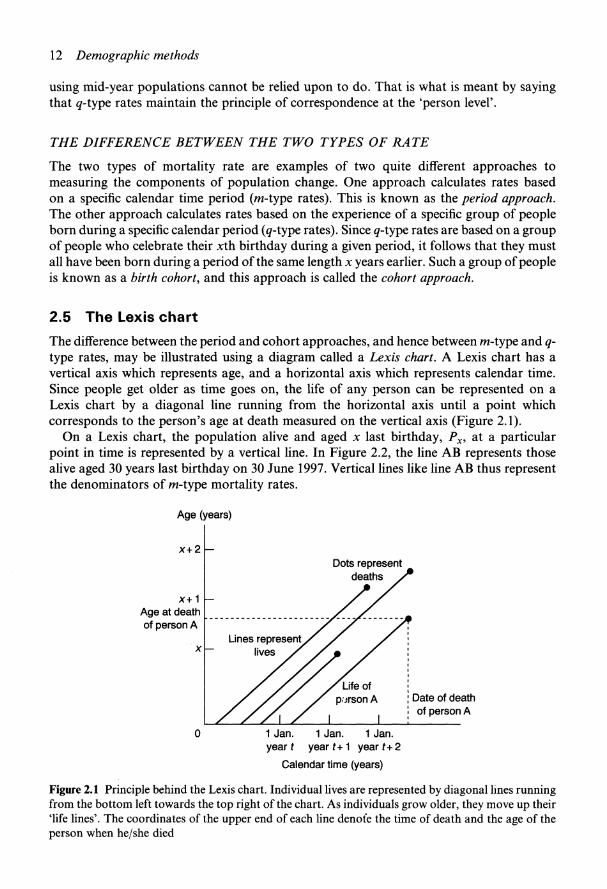
The difference between the period and cohort approaches, and hence between w-type and q-type rates, may be illustrated using a diagram called a Lexis chart. A Lexis chart has avertical axis which represents age, and a horizontal axis which represents calendar time.Since people get older as time goes on, the life of any person can be represented on aLexis chart by a diagonal line running from the horizontal axis until a point whichcorresponds to the person's age at death measured on the vertical axis (Figure 2.1).

On a Lexis chart, the population alive and aged x last birthday, Px, at a particularpoint in time is represented by a vertical line. In Figure 2.2, the line AB represents thosealive aged 30 years last birthday on 30 June 1997. Vertical lines like line AB thus representthe denominators of w-type mortality rates.

Figure 2.1 Principle behind the Lexis chart. Individual lives are represented by diagonal lines runningfrom the bottom left towards the top right of the chart. As individuals grow older, they move up their'life lines'. The coordinates of the upper end of each line denote the time of death and the age of theperson when he/she died

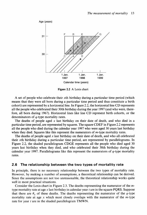
Figure 2.2 A Lexis chart

A set of people who celebrate their .xth birthday during a particular time period (whichmeans that they were all born during a particular time period and thus constitute a birthcohort) are represented by a horizontal line. In Figure 2.2, the horizontal line CD representsall the people who celebrated their 30th birthday during the year 1997 (and who were, there-fore, all born during 1967). Horizontal lines like line CD represent birth cohorts, or thedenominators of #-type mortality rates.

The deaths of people aged x last birthday on their date of death, and who died in aparticular time period, are represented by squares. The square CDEF in Figure 2.2 representsall the people who died during the calendar year 1997 who were aged 30 years last birthdaywhen they died. Squares like this represent the numerators of m-type mortality rates.

The deaths of people aged x last birthday on their date of death, and who all celebratedtheir ;cth birthday during a particular time period, are represented by parallelograms. InFigure 2.2, the shaded parallelogram CDGE represents all the people who died aged 30years last birthday when they died, and who celebrated their 30th birthday during thecalendar year 1997. Parallelograms like this represent the numerators of #-type mortalityrates.

2.6 The relationship between the two types of mortality rate

In principle, there is no necessary relationship between the two types of mortality rate.However, by making a number of assumptions, a theoretical relationship can be derived.Since the assumptions are not too unreasonable, the theoretical relationship works quitewell in most practical situations.

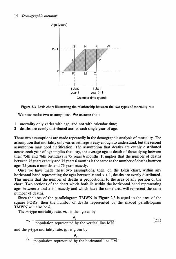
Consider the Lexis chart in Figure 2.3. The deaths representing the numerator of the m-type mortality rate at age x last birthday in calendar year / are in the square PQRS. Supposethat there are Ox of these deaths. The deaths representing the numerator of the g-typemortality rate at age x which most closely overlaps with the numerator of the ra-typerate for year t are in the shaded parallelogram TMWN.

14 Demographic methods

Figure 2.3 Lexis chart illustrating the relationship between the two types of mortality rate

We now make two assumptions. We assume that:

1 mortality only varies with age, and not with calendar time;2 deaths are evenly distributed across each single year of age.

These two assumptions are made repeatedly in the demographic analysis of mortality. Theassumption that mortality only varies with age is easy enough to understand, but the secondassumption may need clarification. The assumption that deaths are evenly distributedacross each year of age implies that, say, the average age at death of those dying betweentheir 75th and 76th birthdays is 75 years 6 months. It implies that the number of deathsbetween 75 years exactly and 75 years 6 months is the same as the number of deaths betweenages 75 years 6 months and 76 years exactly.

Once we have made these two assumptions, then, on the Lexis chart, within anyhorizontal band representing the ages between x and x+l, deaths are evenly distributed.This means that the number of deaths is proportional to the area of any portion of thechart. Two sections of the chart which both lie within the horizontal band representingages between x and x + 1 exactly and which have the same area will represent the samenumber of deaths.

Since the area of the parallelogram TMWN in Figure 2.3 is equal to the area of thesquare PQRS, then the number of deaths represented by the shaded parallelogramTMWN will also be 0X.

The ra-type mortality rate, mx, is then given by

population represented by the horizontal line TM'

population represented by the vertical line MNmx

and the #-type mortality rate, qx, is given by

qx =

(2.1)

The measurement of mortality 15

But, using the assumptions above, the number of deaths in the triangle TMN must be ^9X,and, since all the lives which cross the line TM also cross the line MN, we have

population represented by the vertical line MN + ̂ 0X'

But, from equation (2.1) above,

population represented by the vertical line MN

Thus, substituting from equation (2.3) into equation (2.2), we have

and the 0X cancel to leave

or, as it is often written,

This result is dependent upon the two assumptions we have made. In many practical situa-tions, however, the approximation is satisfactory.

There are certain age groups, though, in which the assumption that deaths are evenlydistributed is not valid. This is particularly true of the first year of life. Most deaths toinfants during the first year of life take place during the first few weeks of that year.Indeed, in low-mortality populations, it is usual for more than half of all the deaths toinfants under the age of 1 year to occur during the first month of life (see Exercise 2.8).Deaths to infants during the first four weeks of life are known as neonatal deaths. Neonataldeaths may be measured using the neonatal death rate, defined as

neonatal death rate =

number of deaths in a given year toinfants aged 28 days or under

number of births in the given year

For example, in the United Kingdom in 1995, there were 732000 live births, and 3070neonatal deaths. The neonatal death rate was therefore equal to 3070/732000, which is0.0042, or 4.2 per thousand births.

2.7 Advantages and disadvantages of the two typesof mortality rate

The two types of mortality rate have their advantages and disadvantages (Table 2.1).Generally speaking, ra-type rates have the advantage of being straightforward to calculatefrom routinely available data. Their disadvantage is that they do not reflect the experienceof'real' people, and, if calculated using mid-year populations, violate the principle of corre-spondence. The advantages and disadvantages of #-type rates are in a sense 'mirror-images'of those of w-type rates.

Qx (2.2)

16 Demographic methods

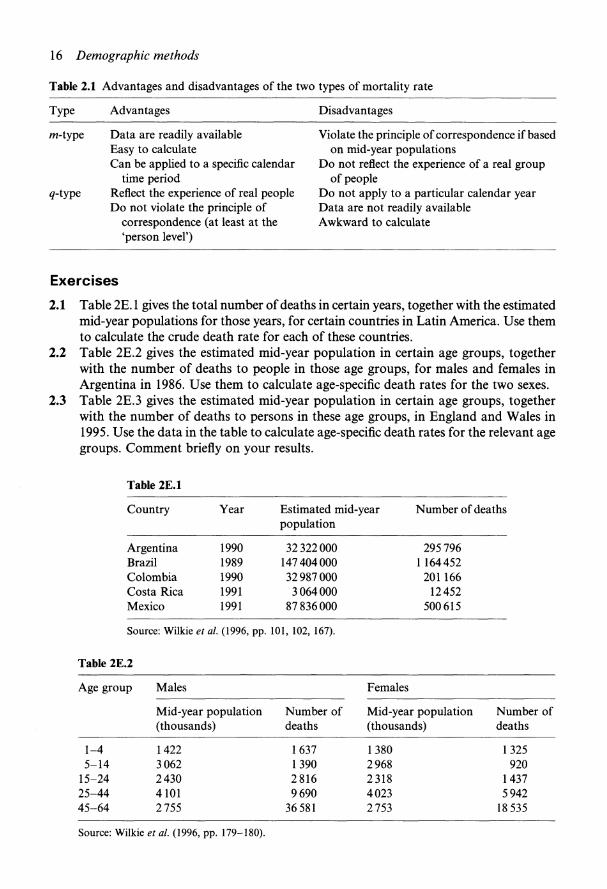
Table 2.1 Advantages and disadvantages of the two types of mortality rate

Type Advantages Disadvantages

m-type

q-type

Data are readily availableEasy to calculateCan be applied to a specific calendar

time periodReflect the experience of real peopleDo not violate the principle of

correspondence (at least at the'person level')

Violate the principle of correspondence if basedon mid-year populations

Do not reflect the experience of a real groupof people

Do not apply to a particular calendar yearData are not readily availableAwkward to calculate

Exercises

2.1 Table 2E. 1 gives the total number of deaths in certain years, together with the estimatedmid-year populations for those years, for certain countries in Latin America. Use themto calculate the crude death rate for each of these countries.

2.2 Table 2E.2 gives the estimated mid-year population in certain age groups, togetherwith the number of deaths to people in those age groups, for males and females inArgentina in 1986. Use them to calculate age-specific death rates for the two sexes.

2.3 Table 2E.3 gives the estimated mid-year population in certain age groups, togetherwith the number of deaths to persons in these age groups, in England and Wales in1995. Use the data in the table to calculate age-specific death rates for the relevant agegroups. Comment briefly on your results.

Table 2E.1

Country

ArgentinaBrazilColombiaCosta RicaMexico

Year

19901989199019911991

Estimated mid-yearpopulation

32322000147404000329870003064000

87836000

Number of deaths

2957961 164452

201 16612452

500615

Source: Wilkie et al. (1996, pp. 101, 102, 167).

Table 2E.2

Age group Males Females

1-45-14

15-2425-4445-64

Mid-year population(thousands)

14223062243041012755

Number ofdeaths

1637139028169690

36581

Mid-year population(thousands)

13802968231840232753

Number ofdeaths

1325920

14375942

18535

Source: Wilkie et al. (1996, pp. 179-180).

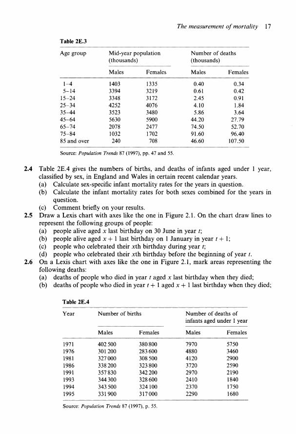
The measurement of mortality 17

Table 2E.3

Age group Mid-year population(thousands)

1-45-14

15-2425-3435-4445-6465-7475-8485 and over

Males

14033394334842523523563020781032240

Females

13353219317240763480590024771702708

Number of deaths(thousands)

Males

0.400.612.454.105.86

44.2074.5091.6046.60

Females

0.340.420.911.843.64

27.7952.7096.40

107.50

Source: Population Trends 87 (1997), pp. 47 and 55.

2.4 Table 2E.4 gives the numbers of births, and deaths of infants aged under 1 year,classified by sex, in England and Wales in certain recent calendar years.(a) Calculate sex-specific infant mortality rates for the years in question.(b) Calculate the infant mortality rates for both sexes combined for the years in

question.(c) Comment briefly on your results.

2.5 Draw a Lexis chart with axes like the one in Figure 2.1. On the chart draw lines torepresent the following groups of people:(a) people alive aged x last birthday on 30 June in year /;(b) people alive aged x + 1 last birthday on 1 January in year / - h i ;(c) people who celebrated their xth birthday during year /;(d) people who celebrated their xih birthday before the beginning of year /.

2.6 On a Lexis chart with axes like the one in Figure 2.1, mark areas representing thefollowing deaths:(a) deaths of people who died in year / aged x last birthday when they died;(b) deaths of people who died in year t + 1 aged x + 1 last birthday when they died;

Table 2E.4

Year Number of births Number of deaths ofinfants aged under 1 year

19711976198119861991199319941995

Males

402500301200327000338 200357830344300343 500331900

Females

380800283 600308 500323 800342200328 600324100317000

Males

79704880412037202970241023702290

Females

57503460290025902190184017501680

Source: Population Trends 87 (1997), p. 55.

18 Demographic methods

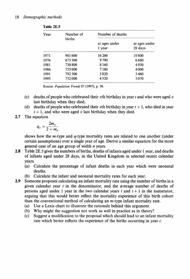
Table 2E.5

Year

197119761981198619911995

Number ofbirths

901 600675 500730800755000792500732000

Number of deaths

at ages under1 year

1620097908160718058204520

at ages under28 days

1080066804930400034603070

Source: Population Trends 87 (1997), p. 50.

(c) deaths of people who celebrated their xth birthday in year / and who were aged xlast birthday when they died;

(d) deaths of people who celebrated their xth birthday in year t + 1 , who died in year/ + 1, and who were aged x last birthday when they died.

2.7 The equation

shows how the m-type and #-type mortality rates are related to one another (undercertain assumptions) over a single year of age. Derive a similar equation for the moregeneral case of an age group of width n years.

2.8 Table 2E.5 gives the numbers of births, deaths of infants aged under 1 year, and deathsof infants aged under 28 days, in the United Kingdom in selected recent calendaryears.(a) Calculate the percentage of infant deaths in each year which were neonatal

deaths.(b) Calculate the infant and neonatal mortality rates for each year.

2.9 Someone proposes calculating an infant mortality rate using the number of births in agiven calendar year t in the denominator, and the average number of deaths ofpersons aged under 1 year in the two calendar years t and t + 1 in the numerator,arguing that this would better reflect the mortality experience of this birth cohortthan the conventional method of calculating an m-type infant mortality rate.(a) Use a Lexis chart to illustrate the rationale behind this argument.(b) Why might the suggestion not work as well in practice as in theory?(c) Suggest a modification to the proposal which should lead to an infant mortality

rate which better reflects the experience of the births occurring in year t.