The Mazur Intersection PropertyIn Banach Spaces And

Related Topics

Pradipta Bandyopadhyaya

Thesis submitted to the Indian Statistical Institute

in partial fulfilment of the requirements

for the award of the degree of

Doctor of Philosophy

CALCUTTA

1991

Acknowledgements

It appears to be customary to begin by thanking one’s supervisor. But I find it

superfluous, particularly since Professor A. K. Roy means much more to me than

merely my supervisor. After all, one normally doesn’t thank his parents for holding

his hands when he is taking his first faltering steps, for teaching him to walk.

Though I consider this entire thesis as a kind of joint venture, Prof. Roy has

allowed me to pass much of it as my own. For the records, only the materials of

Chapter 3 have so far appeared as a joint paper, which too he has permitted me

to include in this thesis without any questions asked.

I joined this Institute as a student more than a decade ago. The list of teachers

who have taught me, nurtured me, encouraged me, made me what I am today, is

naturally bound to read like the whole faculty list. To each of them I owe a lot

and it is impossible for me to choose only few of them for special mention. The

same is also true for the numerous friends and colleagues in the hostel, the division

or outside. Each of them contributed in making this place my “home away from

home”, gave me much-needed moral support. I thank them all.

In the initial days of my research, I had good fortune of many fruitful discus-

sions with Prof. D. van Dulst of University of Amsterdam and Dr. T.S.S.R.K. Rao

of ISI, Bangalore, who were visiting our Institute at that time. My sincere thanks

to both of them.

Last year, I went to New Delhi to participate in a National Seminar and there

I met Dr. D. P. Sinha of Delhi University, who soon became a personal friend. It

is from one of his ideas that the materials of Section 5.3 of this thesis came up.

It’s a pleasure to thank him.

Finally, the manuscript of this thesis was typeset using LATEX. Prof. A. R. Rao

introduced me to LATEX, and Mr. Joydeep Bhanja helped me tailor it according

to my needs. Also, Prof. A. K. Adhikari of the CSU has kindly allowed me to use

the Laser printer there. I am in their debt.

February, 1991 Pradipta Bandyopadhyaya

ii

Contents

1 Introduction 1

2 The MIP for a Family of Closed Bounded Convex Sets 11

2.1. The Set-up and Main Result . . . . . . . . . . . . . . . . . . . 11

2.2. The MIP with Respect to a Norming Subspace F . . . . . . . 18

2.3. A Digression . . . . . . . . . . . . . . . . . . . . . . . . . . . . 23

3 Bochner Lp Spaces and the `p Sums of MIP Spaces 26

3.1. The `p Sums . . . . . . . . . . . . . . . . . . . . . . . . . . . . 26

3.2. Bochner Lp Spaces . . . . . . . . . . . . . . . . . . . . . . . . 28

4 Miscellaneous Results 43

4.1. The Subspace Question . . . . . . . . . . . . . . . . . . . . . . 43

4.2. The MIP and Farthest Points . . . . . . . . . . . . . . . . . . 45

4.3. The MIP in Projective Tensor Product Spaces . . . . . . . . . 48

5 Exposed Points of Continuity and Strongly Exposed Points 62

5.1. The Counterexample . . . . . . . . . . . . . . . . . . . . . . . 62

5.2. A Characterisation Theorem . . . . . . . . . . . . . . . . . . . 64

5.3. A Characterisation of Banach Spaces Containing `1 . . . . . . 67

Reference 69

iii

Chapter 1

Introduction

In the first part of this chapter we explain in general terms the main theme

of this thesis and provide a chapterwise summary of its principal results. The

second part recapitulates some of the known notions and results used in the

subsequent chapters. The numbers given in parentheses correspond to those

in the list of references on page 69.

S. Mazur [40] was the first to consider the following smoothness property

in normed linear spaces, called the Mazur Intersection Property (MIP), or,

more briefly, the Property (I) :

Every closed bounded convex set is the intersection of closed balls

containing it.

He showed that any reflexive Banach space with a Frechet-differentiable norm

has this property.

Later, R. R. Phelps [42] provided a more geometric insight into this prop-

erty by showing that

(a) A normed linear space X has the MIP if the w*-strongly exposed points

of the unit ball B(X∗) of the dual X∗ are norm dense in the unit

sphere S(X∗).

(b) If a normed linear space X has the MIP, every support mapping on X

maps norm dense subsets of S(X) to norm dense subsets of S(X∗).

(c) A finite dimensional normed linear space X has the MIP if and only if

the extreme points of B(X∗) are norm dense in S(X∗).

He also asked whether the sufficient condition (a) is also necessary. To

date, this remains an open question.

1

Nearly two decades later, Phelps’ characterisation (c) was extended by

J. R. Giles, D. A. Gregory and B. Sims [21] to general normed linear spaces,

developing an idea due to F. Sullivan [51], and they proved, inter alia,

Theorem 1.1 For a normed linear space X, the following are equivalent :

(a) The w*-denting points of B(X∗) are norm dense in S(X∗).

(b) X has the MIP.

(c) Every support mapping on X maps norm dense subsets of S(X) to

norm dense subsets of S(X∗).

They also showed that in dual Banach spaces, the MIP implies reflex-

ivity and considered the weaker property that every weak* compact convex

set in a dual space is the intersection of balls (w*-MIP). Investigating the

necessity of Phelps’ condition (a), they showed that it is indeed necessary if,

in addition, the dual X∗ has the w*-MIP, or, X is an Asplund space. They

now asked whether the MIP necessarily implies Asplund. To date, this also

remains open.

Notice that if X is separable and has the MIP, Phelps’ condition (b)

(or, Theorem 1.1(c) above) implies that it has a separable dual and hence is

Asplund. So one asks, is the MIP hereditary, i.e., inherited by subspaces ?

The answer, unfortunately, is no. In Chapter 4, we give an example and

discuss the subspace question in more detail.

However, since the Asplund Property is invariant under equivalent

renorming, a more pertinent question is whether the existence of an equiv-

alent norm with the MIP is hereditary. Some discussions on MIP-related

renorming questions may be found in [9], [47], [54] and [57]. However, in this

work, we do not discuss any renorming problem but concentrate instead on

some of the isometric questions that arise.

Recently, there have appeared several papers dealing with similar inter-

section properties for compact convex sets [54, 47] (called the Property CI),

weakly compact convex sets [57] and compact convex sets with finite affine

dimension [49].

In Chapter 2, we give a unified treatment of the intersection properties

for these diverse classes of sets by considering the MIP for the members of

2

a general family — subject to some mild restrictions — of closed bounded

convex sets in a Banach space and recapture all the known results as special

cases. We also introduce a new condition of separation of convex sets which

is a variant of the following :

Disjoint bounded convex sets are contained in disjoint balls

and this apparently stronger condition turns out to be equivalent to the

intersection property in all known cases. This strengthens the results of Zi-

zler [56]. We should point out that our proofs in this chapter are usually

modifications, refinements and adaptations to our very general set-up of ar-

guments for particular cases to be found in [21], [47] and [54]. This chapter,

which is essentially contained in [3], also provides much of the background

for what follows in the later chapters.

Whitfield and Zizler [55] have also defined the Uniform Mazur Intersection

Property, a property somewhat stronger than the MIP. But in this thesis, we

only briefly touch upon their work.

In Chapter 3, we discuss the question of lifting the MIP and the CI from a

Banach space X to its associated Bochner Lp space and their stability under

`p sums, 1 < p < ∞. In particular, we prove that the `p sum of a family

of Banach spaces has the MIP (or, the CI) if and only if each coordinate

space has it; that the Bochner Lp space for the Lebesgue measure on [0, 1]

always has the CI, while the MIP in X is equivalent to a weaker intersection

property in the Bochner Lp space which turns out to be equivalent to the

MIP if and only if X is Asplund. Most of these results have already appeared

in print in [4].

In Chapter 4, we present a collection of partial results relating to various

aspects of the MIP that raise more question than they answer. Apart from

the subspace question mentioned above, in this chapter we discuss the rela-

tion between the MIP and a farthest point phenomenon that was observed

by K. S. Lau [35], but seems to have passed largely unnoticed since then. Lau

had shown that in a reflexive space the MIP is equivalent to the following :

Every closed bounded convex set is the closed convex hull of its

farthest points.

3

We extend this result to characterise the w*-MIP in w*-Asplund dual spaces

using a result of Deville and Zizler [10]. As far as we know, besides the

work of Tsarkov [53] — who has characterised the MIP in finite-dimensional

spaces in terms of convexity of bounded Chebyshev sets — this is the only

attempt at an intrinsic characterisation of the MIP. We also point out some

new direction of investigation that is indicated by our result.

In this chapter, we also discuss the MIP in projective tensor product

spaces. Ruess and Stegall [46] have shown that the injective tensor product

of two Banach spaces of dimension ≥ 2 never has the MIP. And Sersouri [48]

has shown that in fact there is a two-dimensional compact convex set in

X ⊗ε Y that is not intersection of balls. The situation appears to be much

more difficult for projective tensor product spaces. Here we show that the

projective tensor product of two Banach spaces X and Y never has the

MIP if X and Y are Hilbert spaces or are two-dimensional `p spaces for a

large range of values of p. For this purpose, we characterise the extreme

contractions from `p2 to `q

2 and obtain their closure. The technique used is

similar to [34]. In the process, we reestablish relevant special cases of the

results obtained in [25, 26, 28].

Chapter 5 is somewhat independent of the rest. Here we discuss the

following phenomenon : For a closed bounded convex set K in a Banach

space X and a point xo ∈ K, the following implications are easy to establish :

xo strongly exposed =⇒ xo denting point

⇓ ⇓xo exposed and PC =⇒ xo extreme and PC

where by PC we mean a point of continuity (defined more precisely later).

A recent result (see Theorem 1.5 below) is that xo is denting if and only if

xo is extreme and PC, i.e., the implication down the right hand side above is

reversible. This naturally leads to the conjecture that the implication down

the left hand side above, too, can be reversed, i.e., if xo is exposed and PC

(or, equivalently, xo is an exposed denting point) then xo is strongly exposed.

We show that the conjecture is false by constructing a counterexample in

the Banach space `1 and provide a characterisation of strongly exposed points

4

among points of continuity of a closed bounded convex set. As a corollary,

we deduce that the conjecture is true for the points of weakly compact sets.

We also show that the counterexample, in some sense, is actually typical of

`1, i.e., we characterise Banach spaces containing `1 in terms of the validity

of the above conjecture. We also briefly touch upon the necessity of Phelps’

condition (a) in the light of our characterisation of (w*-) strongly exposed

points. This chapter is a revised version of [2].

Notations, Conventions and

General Preliminaries

General reference to this work are the monographs [7], [13] and [20].

We work only with real Banach spaces. Unless otherwise mentioned, by a

subspace we always mean a norm closed linear subspace. The closed unit

ball and the unit sphere of a Banach space X will be denoted by B(X) and

S(X) respectively. For z ∈ X and r > 0, we denote by Br[z] (resp. Br(z))

the closed (resp. open) ball of radius r and centre z.

For x ∈ S(X), D(x) = f ∈ S(X∗) : f(x) = 1. The set valued map D

is called the duality map and any selection of D is called a support mapping.

For f ∈ S(X∗), we similarly define the inverse duality map as D−1(f) =

x ∈ S(X) : f(x) = 1.For a bounded set K ⊆ X, denote [K] = ∩B : B closed ball containing

K and following Franchetti [19], call a bounded set admissible if K = [K].

In this terminology, a Banach space X has the MIP (resp. the CI) if every

norm closed bounded (resp. norm compact) convex set is admissible.

For K ⊆ X, f ∈ X∗ and α > 0, the set S(K, f, α) = x ∈ K : f(x) >

sup f(K) − α is called the open slice of K determined by f and α. For

A ⊆ X, denote by co(A) (resp. aco(A)) the convex (resp. absolutely convex)

hull of A and by int(A), the norm interior of A. For A ⊆ X, f ∈ X∗,

‖f‖A = sup|f(x)| : x ∈ A, Ao = f ∈ X∗ : ‖f‖A ≤ 1 and for B ⊆ X∗,

A-dia(B) = sup‖b1 − b2‖A : b1, b2 ∈ B. For A1, A2 ⊆ X, dist(A1, A2) =

inf‖x1 − x2‖ : xi ∈ Ai, i = 1, 2. For A ⊆ X, Aσ

denotes the closure of

5

A for the topology σ. Whenever the topology is not specified, we mean the

norm topology.

We identify an element x ∈ X with its canonical image x in X∗∗. Let

K be the image of a closed bounded convex K ⊆ X under this canonical

embedding of X in X∗∗. We denote by K the w*-closure of K in X∗∗. K is

of course a w*-compact convex set.

For a measure space (Ω, Σ, µ) and A ∈ Σ, we denote by χA, the indicator

function of A, and by µ|A the restriction of the measure µ to the σ-field of

measurable subsets of A.

Let X be a real Banach space, let F be a total subspace of X∗ (i.e., F

separates points of X). Let σ denote the σ(X, F ) topology on X. For a

closed bounded convex set K ⊆ X, recall that xo ∈ K is called

(a) a σ-denting point of K if, for each ε > 0, xo 6∈ coσ(K \Bε(xo)).

(b) a σ-point of continuity (σ-PC) for K if the identity map, id : (K, σ) →(K, norm) is continuous at xo.

(c) a very strong extreme point of K if, for every sequence xn of K-valued

Bochner integrable functions on [0, 1] with respect to the Lebesgue

measure, the condition

limn→∞

‖∫ 1

oxn(t)dt− xo‖ = 0 implies lim

n→∞

∫ 1

o‖xn(t)− xo‖dt = 0.

(d) an σ-exposed point of K if there exists f ∈ F such that f exposes xo,

i.e., f(x) < f(xo) for all x ∈ K \ xo.

(e) a σ-strongly exposed point of K if there exists f ∈ F such that f

exposes xo and for any sequence xn ⊆ K, limn

f(xn) = f(xo) implies

that limn‖xn − xo‖ = 0.

In the sequel, whenever σ is the weak topology, i.e., F = X∗, we omit

the prefix σ while referring to the above concepts.

The following lemma is very well-known and can be found in [8, Propo-

sition 25.13] or more recently in [45, Lemma 1.3] :

Lemma 1.2 Let E be a locally convex space, K be a compact convex set in

E and x ∈ K. The following are equivalent :

6

(a) x is an extreme point of K.

(b) The family of open slices containing x forms a local base for the

topology of E at x (relative to K).

In Chapter 5, we note an analogue of this lemma for exposed points.

The following characterisation of a σ-denting point is an immediate con-

sequence of the Hahn-Banach Theorem :

Lemma 1.3 Let X be a Banach space, F be a total subspace of X∗, K be a

closed bounded convex set in X and x ∈ K. The following are equivalent :

(a) x is a σ-denting point of K.

(b) The family of σ-open slices containing x forms a local base for the

norm topology at x (relative to K).

The following lemma is also well-known :

Lemma 1.4 Let K be a closed bounded convex set of a Banach space X.

Then x∗∗ ∈ K is a w*-PC if and only if x∗∗ = x for some x ∈ K and x is

a PC.

The following characterisation of a denting point of a closed bounded

convex set in a Banach space is a consequence of the two lemmas above and

is essentially contained in [38] and [39] :

Theorem 1.5 Let x be an element in a closed bounded convex set K of a

Banach space. Then the following are equivalent :

(a) x is a denting point of K.

(b) x is a w*-denting point of K.

(c) x is a very strong extreme point of K.

(d) For any probability space (Ω, Σ, µ) and any net xα of K-valued

Bochner integrable functions on Ω, the condition

limα‖∫Ω

xα(ω)dµ− x‖ = 0 implies limα

∫Ω‖xα(ω)− x‖dµ = 0.

(e) x is an extreme point of K which is also a PC.

7

Let X be a real Banach space, let F be a norming subspace of X∗ (i.e.,

‖x‖B(F ) = ‖x‖, for all x ∈ X). Then B(X) is σ(X, F )-closed and B(F ) is

w*-dense in B(X∗).

We will need the following generalisation of Lemma 1.4 and Theorem 1.5

(a) ⇐⇒ (e) in the sequel.

Lemma 1.6 Let X be a Banach space, F be a norming subspace of X∗.

(a) A point x∗o ∈ B(X∗) is a w*-PC of B(X∗) if and only if x∗o is a

w*-PC of B(F ).

(b) A point x∗o ∈ B(X∗) is a w*-denting point of B(X∗) if and only if

x∗o is an extreme point and a w*-PC of B(F ).

We will also use the following well-known results :

Lemma 1.7 [42, Lemma 3.1] Let X be a normed linear space and ε > 0. If

f, g ∈ S(X∗) are such that x ∈ B(X) ∩ f−1(0) implies |g(x)| ≤ ε/2, then

either ‖f − g‖ ≤ ε or ‖f + g‖ ≤ ε.

Lemma 1.8 [20, p 205] Let K be a closed bounded convex subset of a Banach

space X. Given f ∈ X∗ \ 0 and xo contained in a slice S of K determined

by f , there exists ε > 0 such that whenever ‖f − g‖ < ε, there is a slice S ′

of K determined by g such that xo ∈ S ′ ⊆ S.

For a Banach space X, a function F : X −→ IR is said to be

(a) Gateaux differentiable at a point x ∈ X if there exists an f ∈ X∗ such

that

limλ→0+

∣∣∣∣∣F (x + λy)− F (x)

λ− f(y)

∣∣∣∣∣ = 0 for all y ∈ B(X) and

(b) Frechet differentiable at x if the convergence is uniform over y ∈ B(X).

In particular, if F is the norm, we have the following duality result :

Theorem 1.9 [20, Theorem 3.5.4] In a Banach space X

(a) the norm is Gateaux differentiable (or smooth) at a point x ∈ S(X)

if and only if D(x) is single-valued and in that case, x w*-exposes D(x)

in B(X∗).

8

(b) the norm is Frechet differentiable at x ∈ S(X) if and only if D(x)

is single-valued and x w*-strongly exposes D(x) in B(X∗).

Recall that a Banach space X is Asplund if every continuous convex

function F : X → IR is Frechet differentiable on a dense Gδ subset of X, and

a dual space X∗ is w*-Asplund if every continuous w*-lower semicontinuous

convex function F : X∗ → IR is Frechet differentiable on a dense Gδ subset

of X∗.

The following characterisation theorem is a classic [7] :

Theorem 1.10 For a Banach space X,

(i) the following are equivalent :

(a) X is Asplund.

(b) Separable subspaces of X have separable dual.

(c) X∗ has the Radon-Nikodym Property (RNP).

(d) X∗ has the RNP with respect to the Lebesgue measure on [0, 1].

(ii) the following are equivalent :

(a) X∗ is w*-Asplund.

(b) X has the RNP.

If X is a Banach space and (Ω, Σ, µ) a measure space, let Lp(µ, X) de-

note the Lebesgue-Bochner function space of p-integrable X-valued functions

defined on Ω, 1 ≤ p < ∞ (see [14]). Recall (from [13]) that if 1p

+ 1q

= 1

(1 < p < ∞), the space Lq(µ, X∗) is isometrically isomorphic to a subspace

of Lp(µ, X)∗ and that they coincide if and only if X∗ has the RNP with

respect to µ. Also recall (from [14] and [31]) that Lp(µ, X)∗ is isometrically

isomorphic to the following two spaces :

(1) Vq(µ, X∗) = the space of all vector measures F : Σ −→ X∗ such that

the q-variation of F is finite, i.e.,

‖F‖q = sup

∑E∈π

‖F (E)‖q

µ(E)qµ(E) : π is a finite partition of Ω

1/q

< ∞,

(2) Lq(µ, X∗; X) = the space of all w*-equivalence classes of X∗-

valued w*-measurable functions h, such that the real-valued function

‖h(·)‖ ∈ Lq(µ, IR).

9

Only the representation given by (1) will be used by us.

[13, Chapter VIII] contains all necessary information on tensor product

spaces. We just recall here that the dual of the projective tensor product,

X⊗π Y , of two Banach spaces X and Y , is L(X, Y ∗), the space of continuous

linear operators from X to Y ∗.

10

Chapter 2

The Mazur IntersectionProperty for a Family of Closed

Bounded Convex Sets

2.1. The Set-up and Main Result

Let X be a real Banach space, let F be a norming subspace of X∗ and let

A = K ⊆ X : K is admissible

ThenA is a family of norm bounded, σ(X, F )-closed convex sets that is closed

under arbitrary intersection, translation and scalar multiplication. Naturally,

A contains all singletons and all closed balls. In this chapter, we denote the

σ(X, F ) topology on X simply by σ.

Taking A as our model, we let C be a family of norm bounded, σ-closed

convex sets with the following properties :

(A1) C is closed under arbitrary intersection, translation and scalar mul-

tiplication.

(A2) C1, C2 ∈ C =⇒ acoσ(C1 ∪ C2) ∈ C.

(A3) C ∈ C, C absolutely convex and f ∈ F =⇒ C ∩ f−1(0) ∈ C.

Note that (A1) implies that C contains all singletons.

Examples : (i) C = all closed bounded convex sets in X, F = X∗

(ii) X = Y ∗, C = all w*-compact convex sets in X, F = Y

(iii) C = all compact convex sets in X, F = any norming subspace

(iv) C = all compact convex sets in X with finite affine dimension,F = any norming subspace

11

(v) C = all weakly compact convex set in X, F = any norming

subspace.

Let F = Co : C ∈ C. Then F is a local base for a locally convex

Hausdorff vector topology τ on X∗, the topology of uniform convergence on

elements of C. Clearly, τ is stronger than the w*-topology on X∗ and weaker

than the norm topology.

Definitions : (1) Denote by Eτ , the set of all extreme points of B(X∗)

which are also points of continuity of the identity map, id : (B(X∗),w*)

−→ (B(X∗), τ).

(2) For C ∈ C, C absolutely convex, ε > 0 and δ > 0, we say that a point

x ∈ S(X) belongs to the set MC,ε,δ(X) if

supyεC,0<λ≤δ

‖x + λy‖+ ‖x− λy‖ − 2

λ< ε

For C = B(X), we write MC,ε,δ(X) simply as Mε,δ(X). Let MC,ε(X) =

∪δ>0MC,ε,δ(X) and for C = B(X) write MC,ε(X) simply as Mε(X), or even

as Mε whenever there is no scope of confusion. Similarly, MC,ε(X) will often

be abbreviated as MC,ε. Notice that ∩ε>0Mε(X) gives the set of points of

S(X) at which the norm is Frechet differentiable.

(3) Hτ = ∩D(MC,ε(X))τ

: C ∈ C, C absolutely convex, C ⊆ B(X)

and ε > 0.

Lemma 2.1 For any absolutely convex C ∈ C, C ⊆ B(X), x ∈ S(X) and

δ > 0, let

d1(C, x, δ) = supyεC,0<λ≤δ

‖x + λy‖+ ‖x− λy‖ − 2

λ

d2(C, x, δ) = C-dia S(B(X∗), x, δ)

d3(C, x, δ) = C-dia [∪D(y) : y ∈ S(X) ∩Bδ(x)]

Then for any α, δ > 0, we have,

(i) d2(C, x, α) ≤ d1(C, x, δ) +2α

δ(ii) d3(C, x, δ) ≤ d2(C, x, δ)

(iii) d1(C, x, δ) ≤ d3(C, x, 2δ)

12

Proof : (i) Fix α, δ > 0. Put d1 = d1(C, x, δ) and d2 = d2(C, x, α).

For each n ≥ 1, we can choose fn, gn ∈ S(B(X∗), x, α) such that

‖fn − gn‖C > d2 − 1n. Choose yn ∈ C such that (fn − gn)(yn) > d2 − 1

n.

Then

‖x + δyn‖+ ‖x− δyn‖ − 2

δ≥ fn(x + δyn) + gn(x− δyn)− 2

δ≥ d2 −

1

n− 2α

δ

Thus, d1 ≥ d2 − 2αδ

.

(ii) immediately follows from the observation that ∪D(y) : y ∈ S(X) ∩Bδ(x) ⊆ S(B(X∗), x, δ).

(iii) Let λ ≤ δ. Observe that for any y ∈ C ⊆ B(X),∥∥∥∥∥ x± λy

‖x± λy‖− x

∥∥∥∥∥ ≤∥∥∥∥∥ x± λy

‖x± λy‖− (x± λy)

∥∥∥∥∥+ λ = |1− ‖x± λy‖ |+ λ

= | ‖x‖ − ‖x± λy‖ |+ λ ≤ 2λ

Let f ∈ D(x + λy

‖x + λy‖) and g ∈ D(

x− λy

‖x− λy‖). Then

‖x + λy‖+ ‖x− λy‖ − 2

λ=

f(x + λy) + g(x− λy)− 2

λ≤ (f − g)(y) ≤ ‖f − g‖C

And we immediately have :

Lemma 2.2 For any absolutely convex C ∈ C, C ⊆ B(X), x ∈ S(X) and

ε > 0, the following are equivalent :

(i) x ∈ MC,ε(X)

(ii) There is a δ ∈ (0, 1) such that C-dia S(B(X∗), x, δ) < ε

(iii) There is a δ ∈ (0, 1) such that C-dia [∪D(y) : y ∈ S(X) ∩Bδ(x)] < ε.

Corollary 2.2.1 For any absolutely convex C ∈ C, C ⊆ B(X) and ε > 0,

MC,ε(X) is an open subset of S(X).

Proof : Follows immediately from the Lemma above and Lemma 1.8.

Remark : In the case of C = B(X), Lemma 2.1 is quantitatively more

precise than Lemma 1 of [55].

Now we have our main result :

13

Theorem 2.3 If X, F and C are as above, consider the following state-

ments :

(a) F ⊆ IR+Eτ

τ

(b) F ⊆ IR+Hτ

τ

(c) If C1, C2 ∈ C are such that there exists f ∈ F with sup f(C1) <

inf f(C2) then there exist disjoint closed balls B1, B2 such that Ci ⊆ Bi,

i = 1, 2.

(d) Every C ∈ C is admissible.

(e) For every norm dense subset A of S(X) and every support mapping

φ : S(X) −→ S(X∗), F ⊆ IR+φ(A)τ.

Then we have (a) ⇒ (b) ⇒ (c) ⇒ (d) ⇒ (e).

(For the reverse implications, see corollaries and remarks at the end of

this section.)

Proof : (a) ⇒ (b) Enough to prove Eτ ⊆ Hτ .

Let f ∈ Eτ . Let C ∈ C, C absolutely convex, C ⊆ B(X) and ε > 0. We

want to prove f ∈ D(MC,ε)τ. Let K ∈ C and 0 < η < ε. We may assume

K ⊆ B(X). Let Ko = acoσ(K ∪ C). Then Ko ⊆ B(X) as B(X) is σ-closed.

Note that Ko ∈ C by (A2).

Since f is an extreme point of the w*-compact convex set B(X∗) and id :

(B(X∗), w∗) → (B(X∗), τ) is continuous at f , it follows from Lemma 1.2 that

w*-slices of B(X∗) containing f form a base for the relative τ -topology at f .

Thus there exist x ∈ S(X) and 0 < δ < 1 such that f ∈ S = S(B(X∗), x, δ)

and Ko-dia(S) < η.

Now, by Lemma 2.2, x ∈ MKo,η ⊆ MC,ε and for any fx ∈ D(x), fx ∈D(MC,ε) and fx ∈ S, so, ‖f − fx‖K ≤ ‖f − fx‖Ko < η.

(b) ⇒ (c) Let C1, C2 ∈ C and f ∈ S(F ) be such that sup f(C1) <

inf f(C2). Let z ∈ X be such that f(z) = 12(sup f(C1) + inf f(C2)) and

put ε = 112

(inf f(C2) − sup f(C1)) > 0. Then, inf f(C2 − z) > 5ε and

inf(−f)(C1− z) > 5ε. We may assume without loss of generality that z = 0,

Ci ⊆ B(X), i = 1, 2 and ‖f‖ = 1. Let K = acoσ(C1 ∪C2), then K ∈ C, K is

absolutely convex and K ⊆ B(X).

14

By (b), there is λ ≥ 0 and g ∈ Hτ such that ‖f − λg‖K < ε. If λ = 0, we

have ‖f‖K < ε and hence, infC2 f < ε, a contradiction. Thus, λ > 0.

Now, g ∈ Hτ ⊆ D(MK,ε/λ)τ. So, we can find x ∈ MK,ε/λ and h ∈ D(x)

such that ‖g − h‖K < ε/λ. By definition, there is a δ > 0 such that

supyεK,0<α≤δ

‖x + αy‖+ ‖x− αy‖ − 2

α<

ε

λ

Choose an integer n > λεδ

. The proof will be complete once we show that

B1 = B(n−1)ε/λ [−nεx/λ] and B2 = B(n−1)ε/λ [nεx/λ] work.

Clearly, B1 and B2 are disjoint. Suppose, if possible, y ∈ C2 and y 6∈ B2.

Then y ∈ K. Take α = λnε

< δ and observe that

‖x + αy‖+ ‖x− αy‖ − 2

α=

‖x + αy‖ − ‖x‖α

+ ‖x

α− y‖ − 1

α

≥ h(y) +(n− 1)ε

λ− nε

λ= h(y)− ε

λ

≥ g(y)− 2ε

λ=

1

λ[λg(y)− 2ε]

>1

λ[f(y)− 3ε] ≥ 1

λ[5ε− 3ε] =

2ε

λ

This contradicts the fact that x ∈ MK,ε/λ. The other inclusion follows sim-

ilarly once we note that K, and hence MK,ε/λ, is symmetric and h ∈ D(x)

implies (−h) ∈ D(−x).

(c) ⇒ (d) Since singletons are in C and every C ∈ C is σ-closed, (d)

follows from (c).

(d) ⇒ (e). (We adapt Phelps’ [42] arguments) Let A be a norm dense

subset of S(X) and φ be a support mapping. Let f ∈ S(F ), K ∈ C and

0 < ε < 1. We may assume K ⊆ B(X) and further that K is absolutely

convex and ‖f‖K > 1 − ε/2 (Let x ∈ B(X) such that f(x) > 1 − ε/2. Let

L = acoσ[x ∪K]. Then L ⊆ B(X), L ∈ C and ‖ · ‖L ≥ ‖ · ‖K). Let u ∈ K

be such that f(u) > 1 − ε/2. Put u′ = εu/4 and D = K ∩ f−1(0). Then

D ∈ C [by (A3)] and u′ 6∈ D. By (c), there exists z ∈ X and r > 0 such that

D ⊆ Br[z] and ‖u′ − z‖ > r.

Let µ = ‖u′ − z‖ − r > 0. Put w = 1r+µ

(ru′ + µz). Then ‖w − z‖ = r.

Put x = 1r(w − z) ∈ S(X). Let C = co[u′ ∪ Br[z]]. Let 0 < δ < µ

(r+µ).

15

If p ∈ Brδ[w], then ‖p − w‖ < rµ(r+µ)

, so, p = w + rµr+µ

· y for some y ∈ X,

‖y‖ < 1. Thus, p = rr+µ

u′ + µr+µ

(z + ry). Now, z + ry ∈ Br(z) and hence,

p ∈ int(C). So, Brδ[w] ⊆ int(C).

Let y ∈ Bδ[x] ∩ A and g = φ(y). Put v = ry + z. Clearly, ‖v − w‖ ≤ rδ,

hence v ∈ int(C) and g(v) = sup g(Br[z]). Now, v ∈ int(C) ⇒ there exists

t ∈ (0, 1) and v′ ∈ Br(z) such that v = tu′ + (1 − t)v′. Thus, g(v) =

tg(u′) + (1 − t)g(v′) < tg(u′) + (1 − t)g(v). Also, 0 ∈ D ⊆ Br[z] =⇒0 ≤ g(v) < g(u′) = 1

4εg(u) ≤ 1

4ε · ‖g‖K . So, 0 < ‖g‖K ≤ ‖g‖ = 1. Put

λ = 1/‖g‖K . Then sup λg(D) ≤ sup λg(Br[z]) = λg(v) < 14ε · ‖λg‖K = ε/4.

By symmetry of D, ‖λg‖D ≤ ε/4.

Now, by Lemma 1.7 applied to the linear space sp(K), spanned by K,

equipped with µK , the gauge or Minkowski functional of K, we have∥∥∥∥∥ f

‖f‖K

+ λg

∥∥∥∥∥K

≤ ε

2or

∥∥∥∥∥ f

‖f‖K

− λg

∥∥∥∥∥K

≤ ε

2

But u ∈ K and ε < 1 implies f(u)/‖f‖K ≥ f(u) > 1 − ε/2 > ε/2 and

λg(u) > 0. Thus, ‖ f

‖f‖K

− λg‖K ≤ ε/2. Then we have

‖f − λg‖K ≤ ε

2+

∥∥∥∥∥ f

‖f‖K

− f

∥∥∥∥∥K

=ε

2+ (1− ‖f‖K) ≤ ε

2+

ε

2= ε

Corollary 2.3.1 If in the set-up of Theorem 2.3, we have that the set

A = x ∈ S(X) : D(x) ∩ Eτ 6= ∅

is norm dense in S(X), then all the statement in Theorem 2.3 are equivalent.

Proof : We simply note that in this case there is a support mapping that

maps A into Eτ and hence, (e) ⇒ (a).

Corollary 2.3.2 [54, 47, 49] In the case of examples (iii), i.e., C = allcompact convex sets in X, F = any norming subspace, and (iv), i.e., C= all compact convex sets in X with finite affine dimension, F = any

norming subspace, all the statements in Theorem 2.3 are equivalent and (c)

can be reformulated as

(c′) Disjoint members of C can be separated by disjoint closed balls.

16

Proof : In example (iii), τ is the bw* topology (see [16] for more on bw*

topology) and in example (iv), τ is the w*-topology on X∗ and in both cases

Fτ

= X∗, so we may as well take F = X∗. Further, as the bw* topol-

ogy agrees with the w*-topology on bounded sets, in both the cases, Eτ =

extreme points of B(X∗). Clearly, in both cases A as in Corollary 2.3.1 is

S(X) and so, in Theorem 2.3 all the statements are equivalent.

Since members of C in both cases are σ-compact, (c) ⇐⇒ (c′).

Remarks : 1. In example (v), i.e., C = all weakly compact convex set

in X, F = any norming subspace, τ is the Mackey topology on X∗ (see [8]

for further information) and again, Fτ

= X∗.

In this case, we do not know whether any of the implications in Theo-

rem 2.3 can be reversed. However, we note that (a) ⇒ (d) in Theorem 2.3

gives a weaker sufficiency condition for MIP for weakly compact sets than

the one used in [57]. And in this case, too, (c) and (c′) of Corollary 2.3.2 are

equivalent.

2. It seems unlikely that, in general, the implications in Theorem 2.3

can be reversed. Nevertheless, it appears to be an interesting and difficult

problem to find conditions on X, F , and C under which this can be done.

In particular, when is the assumption of Corollary 2.3.1 satisfied ? In this

context, the work of Namioka [41] on neighbourhoods of extreme points may

conceivably be relevant.

However, there is yet another situation when the statements can actually

be shown to be equivalent. And particular cases of this yield the character-

isations of MIP and w*-MIP, i.e., examples (i) and (ii). This we take up in

the next section.

3. Note that the subspace F ⊆ X∗ was assumed to be norming in order

to ensure that σ-closure of norm bounded sets remain norm bounded which

is implicit in (A2). However, if (A2) is satisfied, as in examples (iii), (iv)

and (v), for any total subspace F , our results easily carry through with only

minor technical modifications in the proofs.

17

2.2. The MIP with Respect to a Norming

Subspace F

Our standing assumption in this section is that F is a subspace of X∗ such

that

the set TF = x ∈ S(X) : D(x) ∩ S(F ) 6= ∅ is a norm dense

subset of S(X)

(we shall write simply T when there is no confusion). Then F is necessarily

norming. However, one can give examples (see below) of norming subspaces

where this property does not hold. Let C = all norm bounded, σ-closed

convex sets in X. We say that X has F -MIP if every C ∈ C is admissible.

Examples : (i) F = X∗, T = S(X) and we have the MIP.

(ii) X = Y ∗, F = Y , T = D(S(Y )), which is dense by Bishop-Phelps

Theorem [5], and we have the w*-MIP.

Now, since B(X) ∈ C, τ is the norm topology on X∗ and Eτ = w*-

denting points of B(X∗). We need the following reformulation of Lemma

2.2 :

Lemma 2.4 For x ∈ S(X), F, T as above and ε > 0, the following are

equivalent :

(i) x ∈ Mε

(ii) x determines a slice of B(F ) of diameter less than ε

(iii) There exists δ > 0 such that

dia[∪D(y) ∩ S(F ) : y ∈ T ∩Bδ(x)] < ε.

Proof : (i) ⇒ (ii) ⇒ (iii) follows as easy adjustments of Lemma 2.1.

(iii) ⇒ (i) Let δ > 0 be as in (iii). Let do = dia[∪D(y) ∩ S(F ) : y ∈T ∩ Bδ(x)] < ε. Choose δo > 0 such that δ2

o + 2δo < δ and δ2o + 2δo/ε <

(1 − do/ε). Let y ∈ S(X), 0 < λ < δo. Then as in the proof of Lemma 2.1,∥∥∥∥∥ x± λy

‖x + λy‖− x

∥∥∥∥∥ ≤ 2λ.

18

Find x1, x2 ∈ T such that∥∥∥ x+λy‖x+λy‖ − x1

∥∥∥ ≤ λ2 and∥∥∥ x−λy‖x−λy‖ − x2

∥∥∥ ≤ λ2.

Let f1, f2 ∈ S(F ) such that fi ∈ D(xi), i = 1, 2. Observe that ‖xi − x‖ ≤λ2 + 2λ ≤ δ2

o + 2δo < δ, i.e., x1, x2 ∈ T ∩Bδ(x). Thus ‖f1 − f2‖ ≤ do. Now,

0 ≤ 1− f1

(x + λy

‖x + λy‖

)= f1

(x1 −

x + λy

‖x + λy‖

)≤∥∥∥∥∥ x + λy

‖x + λy‖− x1

∥∥∥∥∥ ≤ λ2.

So, f1(x + λy) ≥ (1−λ2)‖x + λy‖. Similarly, f2(x−λy) ≥ (1−λ2)‖x−λy‖.So, we have

‖x + λy‖+ ‖x− λy‖ − 2

λ≤ f1(x + λy) + f2(x− λy)− 2(1− λ2)

λ(1− λ2)

=(f1 + f2)(x)− 2 + λ(f1 − f2)(y) + 2λ2

λ(1− λ2)

≤ ‖f1 − f2‖+ 2λ

1− λ2≤ do + 2λ

1− λ2≤ do + 2δo

1− δ2o

(sincedo + 2λ

1− λ2is increasing in λ). Thus,

supyεS(X),0<λ≤δo

‖x + λy‖+ ‖x− λy‖ − 2

λ≤ do + 2δo

1− δ2o

< ε

by the choice of δo.

Definition : Let DF : T → S(F ) be defined by DF (x) = D(x) ∩ S(F ).

We say that DF is quasi-continuous if for every f ∈ S(F ) and ε > 0, there

exists x ∈ T and δ > 0 such that y ∈ Bδ(x) ∩ T implies DF (y) ⊆ Bε[f ].

Notice that for X = Y ∗ and F = Y , DF is the inverse duality map.

Now, we are in a position to prove :

Theorem 2.5 If X, F and T are as above, the following are equivalent :

(a) The w*-denting points of B(X∗) are norm dense in S(F ).

(b) For every ε > 0, D(Mε) ∩ S(F ) is norm dense in S(F ).

(c) If C1, C2 ∈ C are such that there exists f ∈ F with sup f(C1) <

inf f(C2) then there exist disjoint closed balls B1, B2 such that Ci ⊆ Bi,

i = 1, 2.

(d) X has the F-MIP.

19

(e) DF is quasi-continuous.

(f) For every support mapping φ that maps T into S(F ) and for every

norm dense subset A of T, φ(A) is norm dense in S(F ).

(Observe that since Mε is open and T is dense, D(Mε)∩S(F ) 6= ∅ when-

ever Mε 6= ∅.)Proof : (a) ⇒ (b) Let f be a w*-denting point of B(X∗) and ε > 0. As noted

above f ∈ S(F ). Proceeding as in Theorem 2.3 (we may take K = B(X)

and so, Ko = B(X)), for any 0 < η < ε, there is x ∈ S(X) and α > 0 such

that f ∈ S = S(B(X∗), x, α) and dia(S) < η. Since T is dense in S(X), by

Lemma 1.8, there is y ∈ T and δ > 0 such that f ∈ S ′ = S(B(X∗), y, δ) and

S ′ ⊆ S. Again as in Theorem 2.3, y ∈ Mε ∩T and for any fy ∈ D(y)∩S(F ),

‖fy − f‖ < η.

(b) ⇒ (c) ⇒ (d) ⇒ (f) Just a simplified version of the implication

(b) ⇒ (c) ⇒ (d) ⇒ (e) in Theorem 2.3 where we replace K by B(X).

(e) ⇒ (f) Follows from definitions.

(f) ⇒ (e) Suppose DF is not quasi-continuous. Then there exist f ∈S(F ) and ε > 0 such that for all x ∈ T and δ > 0, there exists y(x, δ) ∈Bδ(x) ∩ T such that DF (y) 6⊆ Bε[f ].

Let A = y(x, δ) : x ∈ T , δ > 0. Then A is dense in T and we can get a

support mapping φ that maps T into S(F ) and φ(A) ∩Bε[f ] = ∅.(e) ⇒ (b) Let f ∈ S(F ) and ε > 0. Let 0 < η < ε/2. By (e), there exists

x ∈ T and δ > 0 such that y ∈ T ∩ Bδ(x) implies D(y) ∩ S(F ) ⊆ Bη[f ].

But then dia[∪D(y) ∩ S(F ) : y ∈ T ∩Bδ(x)] ≤ 2η < ε. So by Lemma 2.4,

x ∈ Mε ∩ T and fx ∈ D(x) ∩ S(F ) implies ‖fx − f‖ < η.

(b) ⇒ (a) For n ≥ 1, let Dn = f ∈ S(F ) : f is contained in a w*-open

slice of B(F ) of diameter < 1n. By Lemma 2.4, D(M1/n) ∩ S(F ) ⊆ Dn.

Thus, for all n ≥ 1, Dn is norm open dense subset of S(F ) and by Baire

Category Theorem, ∩Dn is dense in S(F ). But, it is easy to see that ∩Dn =

w*-denting points of B(X∗).For completeness, we record in full the following immediate consequences,

most of which are well-known results in the MIP literature.

Theorem 2.6 [21, Theorem 2.1 and 3.1] For a Banach space X

20

(1) the following are equivalent :

(a) The w*-denting points of B(X∗) are norm dense in S(X∗).

(b) For every ε > 0, D(Mε(X)) is norm dense in S(X∗).

(c) Whenever C1, C2 are closed bounded convex sets in X with

dist(C1, C2) > 0, there exist disjoint closed balls B1, B2 such that

Ci ⊆ Bi, i = 1, 2.

(d) X has the MIP.

(e) The duality map is quasi-continuous.

(f) Every support mapping maps norm dense subsets of S(X) to norm

dense subsets of S(X∗).

(2) the following are equivalent :

(a) The denting points of B(X) are norm dense in S(X).

(b) For every ε > 0, D−1(Mε(X∗)) is norm dense in S(X).

(c) Disjoint w*-compact convex sets in X∗ can be separated by disjoint

closed balls.

(d) X∗ has the w*-MIP.

(e) The inverse duality map is quasi-continuous.

(f) Every support mapping that maps D(S(X)) into S(X) maps norm

dense subsets of D(S(X)) to norm dense subsets of S(X).

Proof : (1) Let dist(C1, C2) = δ > 0. Let K2 = C2 + Bδ/2B(0). Then C1

and K2 are disjoint closed convex sets and K2 has non-empty interior. Now,

f ∈ X∗ that separates C1 and K2 strictly separates C1 and C2. Thus (1)

follows from Theorem 2.5.

(2) Observe that x : x is a denting point of B(X) = w*-denting points

of B(X∗∗). Now (2) is immediate from Theorem 2.5.

Remark : Since disjoint closed balls always have positive distance, this

result cannot be strengthened. Note that this Theorem and Corllary 2.3.2

considerably strengthen Corollaries on p 341 and p 343 respectively of [56].

In the following proposition, we collect without proof some observations

regarding the MIP. Recall (from [22]) that a norming subspace of X∗ is

minimal if it is contained in all norming subspaces.

21

Proposition 2.7 For a Banach space X

(a) If the norm is Frechet differentiable at all x ∈ S(X), then X has

the MIP and is Asplund. If the norm is smooth at all x ∈ S(X), then

X has the CI.

(b) [42] If X is finite dimensional, then X has the MIP (equivalently,

the CI) if and only if the extreme points of B(X∗) are dense in S(X∗).

In particular, a 2-dimensional space has the MIP if and only if it is

smooth.

(c) [42] If the w*-strongly exposed points of B(X∗) are dense in S(X∗),

X has the MIP.

(d) [21] If X has the MIP and the norm is Frechet differentiable on a

dense subset of S(X), then the w*-strongly exposed points of B(X∗) are

dense in S(X∗). In particular, this happens when X has the MIP and

either X∗ has the w*-MIP or X is Asplund.

(e) [51] If X is separable and has the MIP, then X is Asplund.

(f) If X has the F -MIP, then F is the minimal norming subspace of

X∗. Hence, if X has the MIP, then X∗ contains no proper norming

subspace. In particular, X∗ has the MIP implies X is reflexive.

(g) X has the MIP implies X∗∗ has the w*-MIP.

Remarks : 1. Apropos (d) above, does X has the MIP imply X is

Asplund ? In this context, Sullivan [51] has shown that if for some ε > 0,

Mε = S(X), then X is Asplund.

2. As a strengthening of (f) above, he has also proved that if X is the

range of a norm one projection in a dual space and for some 0 < ε < 1,

D(Mε) is dense in S(X∗), then X is reflexive.

3. On the other hand, Godefroy and Kalton [22] have proved that if X is

the range of a norm one projection in a dual space and every closed bounded

convex set in X is the intersection of finite union of balls, then X is reflexive.

4. Does the minimal norming subspace of the dual, if it exists, always

satisfy our standing assumption of this section ? Does there exist a subspace

22

F of X∗ satisfying our standing assumption that is minimal with respect to

this property ?

5. Is the converse of (g) above true ?

2.3. A Digression

In [21], a version of Lemma 2.4 was proved for X = Y ∗, F = Y using

the Bollobas’ estimates for the Bishop-Phelps Theorem (see [5] and [6]).

Specifically, the authors of [21] used the fact that in this case the following

holds :

(∗)

For every x ∈ S(X) and every sequence fn ⊆ S(F ) such

that fn(x) −→ 1, there exists a sequence xn ⊆ T and

fxn ∈ D(xn) ∩ S(F ) such that ‖xn − x‖ → 0 and ‖fxn − fn‖ → 0.

In fact, one can show that in this situation, the following stronger property

holds (see [20]) :

(∗∗)

For every x ∈ S(X), f ∈ S(F ) and ε > 0 with f(x) > 1− ε2

there exists y ∈ T and fy ∈ D(y) ∩ S(F ) such that ‖x− y‖ ≤ ε

and ‖f − fy‖ ≤ ε.

Using the fact that (∗∗) holds for F = X∗, one can show that (∗∗) also

holds if F is an L-summand in X∗, i.e., there is a projection P on X∗ with

P (X∗) = F such that for any f ∈ X∗, ‖f‖ = ‖Pf‖ + ‖f − Pf‖. Here is a

quick proof.

Let x ∈ S(X), f ∈ S(F ) and 0 < ε < 1 be given such that f(x) > 1− ε2.

Then there exists y ∈ S(X) and y∗ ∈ D(y) such that ‖x − y‖ ≤ ε and

‖f − y∗‖ ≤ ε. Note that ‖f − Py∗‖ ≤ ‖f − y∗‖ ≤ ε < 1, so that Py∗ 6= 0. If

y∗ = Py∗, we are done. Otherwise observe that

1 = ‖y∗‖ = ‖Py∗‖+ ‖y∗ − Py∗‖ and

1 = y∗(y) = Py∗(y) + (y∗ − Py∗)(y)

= ‖Py∗‖(

Py∗

‖Py∗‖

)(y) + ‖y∗ − Py∗‖

(y∗ − Py∗

‖y∗ − Py∗‖

)(y) ≤ 1

23

Thus, Py∗/‖Py∗‖ ∈ D(y) ∩ S(F ), whence y ∈ T . Further∥∥∥∥∥f − Py∗

‖Py∗‖

∥∥∥∥∥ ≤ ‖f − Py∗‖+ (1− ‖Py∗‖)

= ‖f − Py∗‖+ ‖y∗ − Py∗‖ = ‖f − y∗‖ ≤ ε

Clearly, if (∗∗) holds for the pair (X,F ), it also holds for the pair (F, X).

In particular, (∗∗) holds for each of the following :

(1) X = C[0, 1], F = discrete measures on [0, 1],

(2) X = C[0, 1], F = absolutely continuous measures on [0, 1],

(3) X = L1[0, 1], F = C[0, 1].

So, in these cases, (∗) also holds and the proof of [21] can be used to prove

Lemma 2.4.

Another example of a situation in which (∗∗) is satisfied is furnished by

Proposition 3.4 in the next chapter.

However, one can construct examples (see below) to show that (∗∗) does

not, in general, follow from the density of T in S(X). It would be interesting

to know whether (∗) does. Also it would be interesting to find general suffi-

ciency conditions for (∗∗) to hold which would cover at least the case X = Y ∗

and F = Y . In particular, is the following obviously necessary condition also

sufficient for (∗∗) to hold :

T is dense in S(X) and D(T ) ∩ S(F ) is dense in S(F ) ?

But these may be difficult problems.

Example : Let X be a non-reflexive Banach space. Let F ⊆ X∗ be a

norming subspace which is an L-summand in X∗. Let P be the corresponding

L-projection. Let fo ∈ (I−P )(X∗) such that ‖fo‖ = 1 and fo does not attain

its norm on B(X). Let F1 = F⊕1 IRfo. Then F1 is a norming subspace of X∗

and fo ∈ S(F1). Let 0 < ε < 12. Suppose there exists x ∈ S(X), g ∈ S(F1)

such that ‖fo − g‖ < ε and g(x) = 1.

Now, g = f + αfo for some f ∈ F , α ∈ IR. We have

1 = ‖g‖ = ‖f‖+ ‖αfo‖ = ‖f‖+ |α|

24

If α = 0, g = f and we have

ε > ‖fo − g‖ ≥ ‖Pfo − Pg‖ = ‖g‖ = 1

So, α 6= 0. Also, f = 0 implies g = αfo and so fo(x) = ±1, a contradiction

as fo does not attain its norm. Thus, f 6= 0.

But then,

1 = g(x) = f(x) + αfo(x) = ‖f‖ · f

‖f‖(x) + |α|fo

(αx

|α|

)≤ ‖f‖+ |α| = 1

This implies fo(αx/|α|) = 1. Again, a contradiction.

As noted earlier, the pair (X,F ) satisfies (∗∗), so TF is dense in S(X)

and D(TF ) ∩ S(F ) is dense in S(F ). Now, clearly TF1 ⊇ TF , but the above

shows D(TF1) ∩ S(F1) is not dense in S(F1). Consequently, though TF1 is

dense in S(X), (∗∗) is not satisfied.

Also, interchanging the roles of X and F1, the above shows that though

X is a norming subspace of F ∗1 , T

X= D(TF1) ∩ S(F1) is not dense, i.e., our

standing assumption is not satisfied.

Finally, we note that X = C[0, 1], F = discrete measures on [0, 1] and

fo = λ|[0,1/2]− λ|[1/2,1] satisfies the hypothesis of the above example, where λ

denotes the Lebesgue measure.

25

Chapter 3

Bochner Lp Spaces andThe `p Sums of Banach Spaces

with the MIP

3.1. The `p Sums

That the existence of an equivalent renorming with the MIP or the CI is

stable under co or `p sums for 1 < p < ∞ was established by A. Sersouri

[47] using a renorming result for the MIP by R. Deville [9] and for the CI by

himself [47].

We can, however, prove the following direct result for the `p sums,

1 < p < ∞.

Theorem 3.1 Let Xα : α ∈ Γ be a family of Banach spaces. Then the

space X = (⊕α∈ΓXα)`p with the usual `p-norm (1 < p < ∞) has the MIP

(resp. the CI) if and only if for all α ∈ Γ, the space Xα has the MIP (resp.

the CI).

Recall that if X is as above, X∗ = (⊕α∈ΓX∗α)`q , where 1

p+ 1

q= 1. The

following lemma is well-known :

Lemma 3.2 [50, p 154] Let Xα and X be as above. A point x = (xα) ∈S(X) is an extreme point of B(X) if and only if for all α ∈ Γ, either xα = 0

or xα/‖xα‖ is an extreme point of B(Xα).

[50] also contains similar characterisations of various other types of ex-

treme points of B(X). In the dual situation, we can prove

26

Lemma 3.3 Let Xα and X be as above. A point x∗ = (x∗α) ∈ S(X∗) is

a w*-denting point of B(X∗) if and only if for every α, either x∗α = 0 or

x∗α/‖x∗α‖ is a w*-denting point of B(X∗α).

We postpone the proof of Lemma 3.3 till the next section where similar

results will be proved in a more general setting.

Proof of Theorem 3.1 : (The MIP) : Let for all α ∈ Γ, Xα have the MIP.

Let x∗ = (x∗α) ∈ S(X∗). Fix ε > 0. Let Γo = α ∈ Γ : x∗α 6= 0. For α ∈ Γo,

x∗α/‖x∗α‖ ∈ S(X∗α) and since Xα has the MIP, there exists y∗α, a w*-denting

point of B(X∗α), such that

∥∥∥y∗α − x∗α‖x∗α‖

∥∥∥ < ε. Define z∗ = (z∗α) by

z∗α =

‖x∗α‖y∗α if α ∈ Γo

0 otherwise

By Lemma 3.3, z∗ is a w*-denting point of B(X∗) and ‖x∗ − z∗‖q < ε.

Conversely, if X has the MIP, let αo ∈ Γ and x∗αo∈ S(X∗

αo). Fix 0 < ε < 1.

The point x∗ = (x∗α) defined by

x∗α =

x∗αoif α = αo

0 otherwise

is in S(X∗) and hence there exists y∗, a w*-denting point of B(X∗), such

that ‖x∗ − y∗‖q < ε.

Clearly, ‖x∗αo− y∗αo

‖ < ε < 1 and so, y∗αo6= 0. Also, by Lemma 3.3,

y∗αo/‖y∗αo

‖ is a w*-denting point of B(X∗αo

). Now,∥∥∥∥∥x∗αo−

y∗αo

‖y∗αo‖

∥∥∥∥∥ ≤ ‖x∗αo− y∗αo

‖+ |1− ‖y∗αo‖ | < ε + | ‖x∗αo

‖ − ‖y∗αo‖ |

< ε + ‖x∗αo− y∗αo

‖ < 2ε

Hence, Xαo has the MIP.

(The CI ) : Let for all α ∈ Γ, Xα have the CI.

Let x∗ = (x∗α) ∈ S(X∗). Let K be a compact set in X. We may assume

K ⊆ B(X).

Let πα : X −→ Xα be the co-ordinate projection. Then Kα = πα(K) is a

compact set in Xα, for all α ∈ Γ. Fix ε > 0. Choose Γo ⊆ Γ, Γo finite, such

27

that ‖x∗χΓ\Γo‖q < ε and for all α ∈ Γo, x∗α 6= 0. For α ∈ Γo, there exists y∗α,

an extreme point of B(X∗α) and aα ≥ 0 such that ‖x∗α − aαy∗α‖Kα < ε‖x∗α‖q,

where ‖z∗α‖Kα = sup|z∗α(kα)| : kα ∈ Kα. Define u∗ = (u∗α) by

u∗α =

aαy∗α if α ∈ Γo

0 otherwise

Clearly, u∗α/‖u∗α‖ = y∗α is an extreme point of B(X∗α). So, by Lemma 3.2,

u∗/‖u∗‖q is an extreme point of B(X∗) and for any k = (kα) ∈ K, we have

|(x∗ − u∗)(k)| = |∑α∈Γ

(x∗α − u∗α)(kα)|

≤∑

α∈Γo

|(x∗α − aαy∗α)(kα)|+∑

α 6∈Γo

|x∗α(kα)|

≤∑

α∈Γo

‖x∗α − aαy∗α‖Kα + (∑

α 6∈Γo

‖x∗α‖q)1/q(∑

α 6∈Γo

‖kα‖p)1/p

≤ ε∑

α∈Γo

‖x∗α‖q + ε(∑

α 6∈Γo

‖kα‖p)1/p ≤ ε[‖x∗‖qq + ‖k‖p] ≤ 2ε

since x∗ ∈ S(X∗) and k ∈ K ⊆ B(X). Hence ‖x∗ − u∗‖K ≤ 2ε.

Conversely, let X have the CI. Let αo ∈ Γ, x∗αo∈ S(X∗

αo), Kαo ⊆ Xαo

compact. Define x∗ ∈ S(X∗) as in the case of the MIP. Define K = (xα) :

xαo ∈ Kαo and xα = 0 for α 6= αo. Clearly, K is compact and for any

z∗ ∈ X∗, ‖z∗‖K = ‖z∗αo‖Kαo

.

Now, the CI in Xαo clearly follows from that in X.

Remark : It follows from Proposition 4.1 of the next chapter that if the

co or the `∞ sum of a family of Banach spaces has the MIP (or the CI), then

each of them has the MIP (the CI). The converse is not true in general as

the finite-dimensional spaces `∞n , n ≥ 1, fail the CI.

See also Proposition 4.2 below.

3.2. Bochner Lp Spaces

Let X be a Banach space, (Ω, Σ, µ) a measure space, 1 < r < ∞. Let

A ⊆ S(X). Define

28

Mr(A) = f ∈ S(Lr(µ, X)) : f is of the form f =n∑

i=1

xiχEiwith n ≥ 1

arbitrary, Ei ∈ Σ and xi/‖xi‖ ∈ A for all i = 1, 2, . . . , n

Pr(A) = f ∈ S(Lr(µ, X)) : f is of the form f =∞∑i=1

xiχEiwith Ei ∈ Σ

and xi = 0 or xi/‖xi‖ ∈ A for all i ≥ 1 and,

Nr(A) = f ∈ S(Lr(µ, X)) : for almost all t ∈ Ω, either f(t) = 0 or

f(t)/‖f(t)‖ ∈ A

Note that Mr(A) ⊆ Pr(A) ⊆ Nr(A) ⊆ S(Lr(µ, X)).

The following results are well-known :

(1) If A = extreme points of B(X) then Nr(A) ⊆ extreme points of

B(Lr(µ, X)). (See, e.g., [52]).

(2) If A = strongly exposed points of B(X) then Nr(A) ⊇ strongly

exposed points of B(Lr(µ, X)) ⊇ Mr(A) ([32, 23, 24]).

(3) If A = denting points of B(X) then Nr(A) = denting points of

B(Lr(µ, X)) [37].

A survey of similar results may be found in [50]. In the dual situation,

we note that :

(1) If A = extreme points of B(X∗) then Nq(A) ⊆ extreme points of

B(Lq(µ, X∗)). In the following we prove a stronger assertion.

(2) Any w*-denting point or w*-strongly exposed point of B(Vq(µ, X∗)),

being a w*-PC, necessarily belongs to Lq(µ, X∗)) (see Proposition 3.4

below). And it is implicit in [32] that if A = w*-strongly exposed

points of B(X∗) then Mq(A) ⊆ w*-strongly exposed points of

B(Lq(µ, X∗)). Below, we prove by different methods, a similar result

for w*-denting points of B(Vq(µ, X∗)), the proof being more involved

than that for w*-strongly exposed points.

But, first we note the following :

Proposition 3.4 Let Y = Lp(µ, X) and F = Lq(µ, X∗), 1 < p < ∞, 1p

+1q

= 1. Then every simple function in S(Y ) is in T , where T = x ∈ Y :

D(x) ∩ S(F ) 6= ∅. So, T is dense in S(Y ), F is norming and we are in the

29

set-up of section 2.2. Moreover, the pair (Y, F ) satisfies (∗∗) as defined in

section 2.3.

Proof : Let x =∑n

i=1 xiχEibe any simple function in S(Y ) and φ : S(X) −→

S(X∗) be any support mapping. Define

Φ(x) =n∑

i=1

‖xi‖p−1φ

(x∗i‖x∗i ‖

)χEi

Then, Φ(x) ∈ S(Lq(µ, X∗)) ⊆ S(Vq(µ, X∗)) and 〈x, Φ(x)〉 = 1. Thus, Φ(x) ∈D(x) ∩ S(F ). This proves the first part of the Proposition.

Now, let x ∈ S(Lp(X)), f ∈ S(Lq(X∗)) and ε > 0 be such that f(x) > 1−ε2. Choose 0 < η < ε such that 0 < η[2(ε+1)−η] < f(x)−(1−ε2). Let z and

g be simple functions in S(Lp(X)) and S(Lq(X∗)) respectively such that ‖x−z‖p < η and ‖f−g‖q < η. Refining the partitions if necessary, we may assume

that there is a finite partition E1, E2, . . . , En of Ω such that z =∑n

i=1 ziχEi

and g =∑n

i=1 z∗i χEiwhere zi ∈ X, z∗i ∈ X∗. Now, g(z) =

∑ni=1 z∗i (zi)µ(Ei) >

f(x) − 2η > 1 − (ε − η)2, by the choice of η. Now, consider the discrete

measure space Ω′ = 1, 2, . . . , n with measure P , where P (i) = µ(Ei). Then

z and g can be isometrically identified with elements of S(Lp(P, X)) and

S(Lq(P, X∗)) respectively. But as P is discrete, Lp(P, X)∗ = Lq(P, X∗) and

so (∗∗) is satisfied, i.e., there exists vectors (y1, y2, . . . , yn) and (y∗1, y∗2, . . . , y

∗n)

in S(Lp(P, X)) and S(Lq(P, X∗)) respectively such that∑n

i=1 y∗i (yi)P (i) = 1

and [∑n

i=1 ‖zi− yi‖pP (i)]1/p ≤ (ε− η) and [∑n

i=1 ‖z∗i − y∗i ‖qP (i)]1/q ≤ (ε− η).

Put y =∑n

i=1 yiχEiand fy =

∑ni=1 y∗i χEi

. Then y ∈ S(Lp(µ, X)), fy ∈S(Lq(µ, X∗)) and fy(y) = 1. Further ‖x − y‖p ≤ (ε − η) + η = ε and

‖f − fy‖q ≤ ε.

The CI

Lemma 3.5 Let X be a Banach space, (Ω, Σ, µ) a measure space and

1 < q < ∞. Let A = extreme points of B(X∗) ⊆ S(X∗). Then

(a) Mq(A) = Mq(S(X∗))∩ extreme points of B(Vq(µ, X∗)).

(b) Pq(A) = Pq(S(X∗))∩ extreme points of B(Vq(µ, X∗)).

30

Proof : We prove (a), the proof of (b) being an easy adjustment.

Let F =∑n

i=1 x∗i χAi∈ Mq(A). Suppose that there exist G1, G2 ∈

B(Vq(µ, X∗)) with F = 12(G1 + G2).

We will prove that F = G1 = G2, i.e., for any E ∈ Σ with µ(E) > 0,

F (E) = G1(E) = G2(E). Fix any such E ∈ Σ. Put Ao = Ω \ (∪ni=1Ai).

Then π = Ao, A1, . . . , An is a partition of Ω. For i = 0, 1, . . . , n, define

Ei1 = E ∩ Ai and Ei2 = Ec ∩ Ai. Put x∗o = 0.

Now, for any i = 0, 1, . . . , n and j = 1, 2 with µ(Eij) 6= 0, we have

x∗i µ(Eij) = F (Eij) = 12[G1(Eij) + G2(Eij)] or,

x∗i =1

2

[G1(Eij) + G2(Eij)

µ(Eij)

]

So,

‖x∗i ‖ ≤1

2

[‖G1(Eij)‖+ ‖G2(Eij)‖

µ(Eij)

]and hence

‖x∗i ‖q ≤ 1

2

[‖G1(Eij)‖q + ‖G2(Eij)‖q

µ(Eij)q

]by the convexity of the map t −→ tq (q > 1). But then

1 = ‖F‖qq =

n∑i=0

‖x∗i ‖qµ(Ai)

=n∑

i=0

2∑j=1

‖x∗i ‖qµ(Eij) =∑

(i,j):µ(Eij) 6=0‖x∗i ‖qµ(Eij)

≤ 1

2

∑µ(Eij) 6=0

‖G1(Eij)‖q

µ(Eij)qµ(Eij) +

∑µ(Eij) 6=0

‖G2(Eij)‖q

µ(Eij)qµ(Eij)

≤ 1

2[‖G1‖q

q + ‖G2‖qq] ≤ 1

So, we must have

‖x∗i ‖q =1

2

[‖G1(Eij)‖q + ‖G2(Eij)‖q

µ(Eij)q

]for all i, j with µ(Eij) 6= 0

Then the strict convexity of the map t −→ tq gives

‖x∗i ‖ =‖G1(Eij)‖

µ(Eij)=‖G2(Eij)‖

µ(Eij)whenever µ(Eij) 6= 0

31

Thus,

x∗i‖x∗i ‖

=1

2

[G1(Eij)

‖G1(Eij)‖+

G2(Eij)

‖G2(Eij)‖

]whenever µ(Eij) 6= 0

Now, the extremality of x∗i /‖x∗i ‖ implies

x∗i‖x∗i ‖

=G1(Eij)

‖G1(Eij)‖=

G2(Eij)

‖G2(Eij)‖

whence

x∗i =G1(Eij)

µ(Eij)=

G2(Eij)

µ(Eij)whenever µ(Eij) 6= 0

So,

F (E) =n∑

i=0

x∗i µ(Ei1) =n∑

i=0

G1(Ei1) = G1(E)

Similarly, F (E) = G2(E).

The reverse inclusion being obvious, this completes the proof.

Theorem 3.6 For any Banach space X, any finite non-atomic measure

space (Ω, Σ, µ) and 1 < p < ∞, the space Lp(µ, X) has the CI.

Proof : Let τ denote the topology on Vq(µ, X∗) of uniform convergence on

compact subsets of Lp(µ, X). By Proposition 3.4, B(Lq(µ, X∗)) is w*-dense

in B(Vq(µ, X∗)), so Lq(µ, X∗) is τ -dense in Vq(µ, X∗), and simple functions

are norm dense in Lq(µ, X∗). Thus it suffices, by Lemma 3.5(a), to show

that given any simple function F ∈ S(Lq(µ, X∗)), any compact subset K

of Lp(µ, X) and any ε > 0, there exists a function F1 ∈ Mq(A) such that

‖F − F1‖K < ε, where A = extreme points of B(X∗) ⊆ S(X∗).

Now, since K is compact and simple functions are dense in Lp(µ, X),

there exists simple functions g1, g2, . . . , gm such that K ⊆ ∪mi=1Bε/4(gi).

Suppose we have found a function F1 ∈Mq(A) such that |(F−F1)(gj)| < ε/2

for all j = 1, 2, . . . ,m. Then for any g ∈ K, there exists gj such that

‖g − gj‖p < ε/4. So, |(F − F1)(g)| ≤ |(F − F1)(gj)| + |(F − F1)(g − gj)| ≤12ε + (‖F‖q + ‖F1‖q) · ‖g − gj‖p ≤ 1

2ε + 2 · 1

4ε = ε, since ‖F‖q = ‖F1‖q = 1.

Therefore we may as well assume K is a finite set g1, g2, . . . , gm. Fur-

ther, passing to finer partitions if necessary, we may assume there exists a

32

partition A1, A2, . . . , An of Ω such that µ(Ai) > 0 for all i = 1, 2, . . . , n and

each of the functions g1, g2, . . . , gm and F take constant values on each Ai,

i.e., the functions g1, g2, . . . , gm and F have the form F =∑n

i=1 αix∗i χAi

with

x∗i ∈ S(X∗) for all i = 1, 2, . . . , n and gj =∑n

i=1 xijχAifor all j = 1, 2, . . . ,m,

where some of the αi’s and xij’s may be zero and the αix∗i ’s and xij’s need

not all be distinct. Then,

F (gj) =n∑

i=1

αix∗i (xij)µ(Ai) for all j = 1, 2, . . . ,m

Now, µ is finite implies ‖F‖1 =∑n

i=1 |αi|µ(Ai) < ∞. Fix 0 < η < ε/‖F‖1.

Since B(X∗) is w*-compact and convex, by the Krein-Milman Theorem we

have :

for each i = 1, 2, . . . , n, there exists λik ≥ 0, k = 1, 2, . . . , N with∑Nk=1 λik = 1 and x∗i1, x

∗i2, . . . , x

∗iN , extreme points of B(X∗) such

that

|(x∗i −N∑

k=1

λikx∗ik)(xrs)| < η for all r = 1, 2, . . . , n, s = 1, 2, . . . ,m.

Since µ is non-atomic, for each i = 1, 2, . . . , n, there is a partition Ai1,

Ai2, . . . , AiN of Ai such that µ(Aik) = λikµ(Ai) for all k = 1, 2, . . . , N .

Define

F1 =n∑

i=1

N∑k=1

αix∗ikχAik

Then

‖F1‖qq =

n∑i=1

|αi|qN∑

k=1

µ(Aik) =n∑

i=1

|αi|qµ(Ai) = ‖F‖qq = 1

and since each x∗ik ∈ A, F1 ∈Mq(A). Further, for all j = 1, 2, . . . ,m

F1(gj) =n∑

i=1

N∑k=1

αix∗ik(xij)µ(Aik) =

n∑i=1

N∑k=1

αix∗ik(xij)λikµ(Ai)

=n∑

i=1

αiµ(Ai)(N∑

k=1

λikx∗ik)(xij)

and so,

|(F − F1)(gj)| = |n∑

i=1

αiµ(Ai)[x∗i −

N∑k=1

λikx∗ik](xij)|

33

≤n∑

i=1

|αi| · µ(Ai) · |[x∗i −N∑

k=1

λikx∗ik](xij)|

≤ ηn∑

i=1

|αi|µ(Ai) = η‖F‖1 < ε

Remarks : 1. This shows that the CI is indeed much weaker than

smoothness, as Lp(µ, X) is smooth if and only if X is (see [36]).

2. If the existence of an equivalent CI renorming is hereditary, it would

follow from Theorem 3.6 that every Banach space admits an equivalent CI

renorming. This was also noted by Sersouri [47], although in a different

context.

The MIP

Coming to the question of the MIP, we need the following well-known result :

Lemma 3.7 [50, p 158] Let (Ω, Σ, µ) be a measure space, X a Banach space

and 1 ≤ p < ∞. For fn and f in Lp(µ, X), if ‖fn‖p −→ ‖f‖p and fn −→ f

a.e. [µ], then ‖fn − f‖p −→ 0.

Lemma 3.8 Let X be a Banach space, (Ω, Σ, µ) a measure space and

1 < p < ∞, 1p

+ 1q

= 1. Let A = w*-denting points of B(X∗) ⊆ S(X∗).

Then Pq(A) = Pq(S(X∗))∩ w*-denting points of B(Vq(µ, X∗)).

Proof : Let g =∑∞

i=1 x∗i χEi∈ Pq(A). Then by Lemma 3.5(b), g is an

extreme point of B(Vq(µ, X∗)). So, by Lemma 1.6, it suffices to show that g

is a w*-PC of B(Lq(µ, X∗)), i.e., to prove that if gα ⊆ B(Lq(µ, X∗)) is a

net such that gαw∗−→ g then ‖gα − g‖q −→ 0.

Put Eo = Ω \ ∪∞i=1Ei. Then gαχEo

w∗−→ gχEo = 0 and gαχΩ\Eo

w∗−→gχΩ\Eo = g. Now, by the w*-lower semicontinuity of the norm we have :

1 = ‖g‖q ≤ lim infα

‖gα‖q ≤ lim supα

‖gα‖q ≤ 1

and hence

limα‖gα‖q = 1 = ‖g‖q

34

Similarly, we have

limα‖gαχΩ\Eo‖q = 1

Now,

‖gα‖qq = ‖gαχEo‖q

q + ‖gαχΩ\Eo‖qq

so that

lim supα

‖gαχEo‖qq = lim

α(‖gα‖q

q − ‖gαχΩ\Eo‖qq) = 0

Thus, it suffices to show that ‖gαχΩ\Eo − g‖q = 0.

So, we may assume without loss of generality that (Ω, Σ, µ) is σ-finite,

and for almost all t, g(t) 6= 0.

Fix ε > 0, choose N ≥ 1 such that∑∞

i=N+1 ‖x∗i ‖qµ(Ei) < ε. Put F =

∪Ni=1Ei. We have,

‖gχF‖qq ≤ lim inf

α‖gαχF‖q

q ≤ lim supα

‖gαχF‖qq

and,

‖gχΩ\F‖qq ≤ lim inf

α‖gαχΩ\F‖q

q ≤ lim supα

‖gαχΩ\F‖qq

Suppose

‖gχF‖qq < lim sup

α‖gαχF‖q

q

Then there exists a subnet gβα of gα such that

limα‖gβαχF‖q

q = lim supα

‖gαχF‖qq and lim

α‖gβαχΩ\F‖q

q exists.

Then

1 = ‖gαχF‖qq + ‖gαχΩ\F‖q

q < limα‖gβαχF‖q

q + limα‖gβαχΩ\F‖q

q = limα‖gβα‖q

q ≤ 1

a contradiction. So, we have,

‖gχF‖qq = lim

α‖gαχF‖q

q

Similarly,

‖gχΩ\F‖qq = lim

α‖gαχΩ\F‖q

q

35

Now,

‖gα − g‖qq = ‖(gα − g)χF‖q

q + ‖(gα − g)χΩ\F‖qq

≤ ‖(gα − g)χF‖qq + [‖gαχΩ\F‖q + ‖gχΩ\F‖q]

q

≤ ‖(gα − g)χF‖qq + 2q−1[‖gαχΩ\F‖q

q + ‖gχΩ\F‖qq]

(by convexity of the map t → tq).

So, if ‖(gα − g)χF‖q −→ 0, and ε > 0 is given, we can choose αo such

that for all α ≥ αo,

‖(gα − g)χF‖qq < ε and ‖gαχΩ\F‖q

q < ‖gχΩ\F‖qq + ε

i.e., we have for α ≥ αo, ‖gα − g‖qq ≤ ε + 2q−1 · 3ε.

Thus, it suffices to prove ‖(gα − g)χF‖q −→ 0. So, again, without loss

of generality, we may assume µ is finite and g is of the form∑n

i=1 x∗i χEi∈

S(Lq(µ, X∗)) with E1, E2, . . . , En a partition of Ω.

Suppose now, that ‖gα− g‖q 6→ 0. Then there exists εo > 0 and a subnet

gβα with βα ≥ α for all α, such that ‖gβα−g‖q ≥ εo for all α. For notational

simplicity, put Gα = gβα . Then Gα ∈ B(Lq(µ, X∗)) for all α, Gαw∗−→ g and

‖Gα − g‖q ≥ εo for all α.

As noted earlier,

limα‖Gα‖q = 1 = ‖g‖q (1)

Fix A ∈ Σ, µ(A) > 0. Put Ai1 = A ∩ Ei and Ai2 = Ei \ Ai1. Fix Aij

such that µ(Aij) > 0. For any x ∈ X, xχAij∈ Lp(µ, X), so, 〈xχAij

, Gα〉 −→〈xχAij

, g〉, i.e., 〈x,∫Aij

Gαdµ〉 −→ 〈x, x∗i 〉µ(Aij). This implies

1

µ(Aij)

∫Aij

Gαdµw∗−→ x∗i

whence

‖x∗i ‖ ≤ lim infα

1

µ(Aij)‖∫

Aij

Gαdµ‖ ≤ lim infα

1

µ(Aij)

∫Aij

‖Gα‖dµ

≤ lim infα

[1

µ(Aij)

∫Aij

‖Gα‖qdµ

]1/q

(2)

36

Thus, we have

‖x∗i ‖qµ(Aij) ≤ lim infα

∫Aij

‖Gα‖qdµ for all i, j

Adding, we get

1 = ‖g‖qq =

n∑i=1

2∑j=1

‖x∗i ‖qµ(Aij) ≤n∑

i=1

2∑j=1

lim infα

∫Aij

‖Gα‖qdµ

≤ lim infα

n∑i=1

2∑j=1

∫Aij

‖Gα‖qdµ = lim infα

‖Gα‖qq ≤ 1

So,

‖x∗i ‖qµ(Aij) = lim infα

∫Aij

‖Gα‖qdµ for all i, j

Suppose, for some io, jo, we have

‖x∗io‖qµ(Aiojo) < lim sup

α

∫Aiojo

‖Gα‖qdµ

Then,

‖x∗io‖qµ(Aiojo) < lim sup

α

∫Ω‖Gα‖qdµ−

∑(i,j) 6=(io,jo)

∫Aij

‖Gα‖qdµ

= 1− lim inf

α

∑(i,j) 6=(io,jo)

∫Aij

‖Gα‖qdµ

≤ 1−∑

(i,j) 6=(io,jo)

lim infα

∫Aij

‖Gα‖qdµ

= 1−∑

(i,j) 6=(io,jo)

‖x∗i ‖qµ(Aij)

making

1 = ‖g‖qq =

n∑i=1

2∑j=1

‖x∗i ‖qµ(Aij) < 1

So, we must have

‖x∗i ‖qµ(Aij) = limα

∫Aij

‖Gα‖qdµ for all i, j

Now, by (2) above and by the lim sup-version of (2) we have that for all i, j,

‖x∗i ‖µ(Aij) = limα

∫Aij

‖Gα‖dµ

37

Thus,∫A‖g(t)‖dµ =

n∑i=1

‖x∗i ‖µ(Ai1) = limα

n∑i=1

∫Ai1

‖Gα(t)‖dµ = limα

∫A‖Gα(t)‖dµ

Since A ∈ Σ was arbitrary with µ(A) > 0, we have that for all A ∈ Σ with

µ(A) > 0,

limα

∫A‖Gα(t)‖dµ =

∫A‖g(t)‖dµ

whence, in Lq(µ, IR), ‖Gα(·)‖ w∗−→ ‖g(·)‖. Now, since the space Lq(µ, IR) is

uniformly convex and ‖g(·)‖ ∈ S(Lq(µ, IR)), ‖g(·)‖ is a w*-denting point of

B(Lq(µ, IR)) and hence a w*-PC. So, we have∫Ω| ‖Gα(t)− ‖g(t)‖ |qdµ −→ 0 (3)

Again, fix Aij such that µ(Aij) > 0. Then

1

µ(Aij)

∫Aij

Gαdµw∗−→ x∗i

and1

µ(Aij)

∫Aij

‖Gα‖dµ −→ ‖x∗i ‖

so ∫Aij

Gαdµ∫Aij‖Gα‖dµ

w∗−→ x∗i‖x∗i ‖

Since x∗i /‖x∗i ‖ is a w*-PC of B(X∗), this means∥∥∥∥∥∥ x∗i‖x∗i ‖

−∫Aij

Gαdµ∫Aij‖Gα‖dµ

∥∥∥∥∥∥ −→ 0 or

∥∥∥∥∥ x∗i‖x∗i ‖

−∫Aij

Gαdµ

µ(Aij)‖x∗i ‖

∥∥∥∥∥ −→ 0 (as α −→∞)

Choose a net εα such that εα > 0 for all α and εα −→ 0. We have∥∥∥∥∥∫

Aij

Gα(t)

‖Gα(t)‖+ εα

dµ−∫

Aij

Gα(t)

‖x∗i ‖dµ

∥∥∥∥∥=

∥∥∥∥∥∫

Aij

Gα(t)

[‖x∗i ‖ − ‖Gα(t)‖ − εα

‖x∗i ‖(‖Gα(t)‖+ εα)

]dµ

∥∥∥∥∥≤ 1

‖x∗i ‖

∫Aij

| ‖x∗i ‖ − ‖Gα(t)‖ − εα|dµ

≤ 1

‖x∗i ‖

µ(Aij)

1

µ(Aij)

∫Aij

| ‖g(t)‖ − ‖Gα(t)‖ |qdµ

1/q

+ µ(Aij)εα

≤ µ(Aij)

‖x∗i ‖

1

µ(Aij)

∫Aij

| ‖g(t)‖ − ‖Gα(t)‖ |qdµ

1/q

+ εα

38

Now, by (3) and as εα −→ 0, we conclude that∥∥∥∥∥∫

Aij

Gα(t)

‖Gα(t)‖+ εα

dµ−∫

Aij

Gα(t)

‖x∗i ‖dµ

∥∥∥∥∥ −→ 0

whence ∥∥∥∥∥ x∗i‖x∗i ‖

− 1

µ(Aij)

∫Aij

Gα(t)

‖Gα(t)‖+ εα

dµ

∥∥∥∥∥ −→ 0

Now, x∗i /‖x∗i ‖ is a w*-denting, and hence denting, point of B(X∗), so by

Theorem 1.5(d), we get

1

µ(Aij)

∫Aij

∥∥∥∥∥ x∗i‖x∗i ‖

− Gα(t)

‖Gα(t)‖+ εα

dµ

∥∥∥∥∥ −→ 0 (4)

Now, ∫Aij

‖x∗i −Gα(t)‖dµ

= ‖x∗i ‖∫

Aij

∥∥∥∥∥ x∗i‖x∗i ‖

− Gα(t)

‖Gα(t)‖+ εα

+Gα(t)

‖Gα(t)‖+ εα

− Gα(t)

‖x∗i ‖

∥∥∥∥∥ dµ

≤ ‖x∗i ‖[∫

Aij

∥∥∥∥∥ x∗i‖x∗i ‖

− Gα(t)

‖Gα(t)‖+ εα

∥∥∥∥∥ dµ

+∫

Aij

‖Gα(t)‖‖Gα(t)‖+ εα

· | ‖x∗i ‖ − ‖Gα(t)‖ |+ εα

‖x∗i ‖dµ

]

The first term of the sum goes to zero by (4) and the second by (3). Hence

we have ∫Aij

‖x∗i −Gα(t)‖dµ −→ 0 or∫

Aij

‖g(t)−Gα(t)‖dµ −→ 0

Now, since Aij and A were arbitrary, we have actually proved that∫Ω‖g(t)−Gα(t)‖dµ −→ 0

Using this fact and (1), we can choose αn such that both Gαn(t) → g(t)

a.e. [µ] and ‖Gαn‖q → ‖g‖q. Hence, we have, by Lemma 3.7, ‖Gαn−g‖q → 0.

But this contradicts the choice of Gα.The converse follows immediately from Lemma 1.6, Lemma 3.5 and the

observation that if g =∑∞

i=1 xiχEiand y∗α ⊆ B(X∗), y∗α

w∗−→ x∗k/‖x∗k‖ for

some k then gαdef=∑

i6=k x∗i χEi+ ‖x∗k‖y∗αχEk

∈ B(Vq(µ, X∗)) and gαw∗−→ g.

39

Proof of Lemma 3.3 : In the set-up of Lemma 3.8, put X = (⊕α∈ΓXα)`p ,

Ω = Γ, Σ = Power set of Γ and µ = counting measure. Then Lp(µ, X) =

`p(X) and Lp(µ, X)∗ = `q(X∗) = Lq(µ, X∗). Now,

`p(X) = ((xαβ)α∈Γ)β∈Γ :∑α∈Γ

∑β∈Γ

‖xαβ‖p < ∞

Identify X with the subspace ((xαδαβ)α∈Γ)β∈Γ ⊆ `p(X), where

δαβ =

0 if α 6= β

1 if α = β

Then X∗ gets identified with the subspace ((x∗αδαβ)α∈Γ)β∈Γ ⊆ `q(X∗). Ob-

serve that with this identification, a net x∗ρ ⊆ B(X∗) is w*-convergent to

a point x∗o ∈ S(X∗) if and only if the net x∗ρ ⊆ B(`q(X∗)) is w*-convergent

to x∗o ∈ S(`q(X∗)).

Now, Lemma 3.3 follows immediately from Lemma 3.8.

Lemma 3.9 Let X be a Banach space, (Ω, Σ, µ) a probability space and

1 < r < ∞. Let A ⊆ S(X). The following are equivalent :

(a) A is norm dense in S(X).

(b) Mr(A) is norm dense in S(Lr(µ, X)).

(c) Pr(A) is norm dense in S(Lr(µ, X)).

(d) Nr(A) is norm dense in S(Lr(µ, X)).

Proof : Since simple functions in S(Lr(µ, X)) are norm dense (a) implies

(b), and since Mr(A) ⊆ Pr(A) ⊆ Nr(A), (b) =⇒ (c) =⇒ (d).

Now, if x ∈ S(X), xχΩ ∈ S(Lr(µ, X)). So, by (d), there exists a se-

quence fn ⊆ Nr(A) such that ‖fn − xχΩ‖r −→ 0. But then some sub-

sequence fnk converges to xχΩ a.e. [µ]. Now, if t ∈ Ω is such that

‖fnk(t) − xχΩ(t)‖ −→ 0, then ‖fnk

(t) − x‖ −→ 0. Since ‖x‖ = 1, for all

sufficiently large k, ‖fnk(t)‖ 6= 0 and∥∥∥∥∥ fnk

(t)

‖fnk(t)‖

− x

∥∥∥∥∥ −→ 0

As fnk∈ Nr(A), all such fnk

(t)/‖fnk(t)‖ ∈ A. Hence (a) follows.

40

Theorem 3.10 For any Banach space X, finite measure space (Ω, Σ, µ) and

1 < p < ∞ and 1p

+ 1q

= 1, the following are equivalent :

(i) X has the MIP

(ii) Lp(µ, X) has the Lq(µ, X∗)-MIP.

Proof : Define Y , F and T as in Proposition 3.4. Suppose Lp(µ, X) has

the F -MIP. Let A be a norm dense subset of S(X) and φ : S(X) −→S(X∗) be a support mapping. By Lemma 3.9, Mp(A) is norm dense

in S(Lp(µ, X)). Let x =∑n

i=1 xiχEi∈ Mp(A), define Φ(x) as in the

proof of Proposition 3.4. Then, Φ can be extended to a support mapping

Φ : S(Lp(µ, X)) −→ S(Vq(µ, X∗)). Now, Φ maps T into S(F ), Mp(A)

is norm dense in S(Lp(µ, X)) and Lp(µ, X) has the F -MIP, so by Theo-

rem 2.5, Φ(Mp(A)) = Φ(Mp(A)) is norm dense in S(F ). Observe that

Mq(φ(A)) ⊇ Φ(Mp(A)), so that Mq(φ(A)) is norm dense in S(Lq(µ, X∗)).

Now, Lemma 3.9 implies that φ(A) is norm dense in S(X∗).

Since A was an arbitrary dense subset of S(X) and φ an arbitrary support

mapping on X, Theorem 2.6 implies X has the MIP.

Conversely, let X have the MIP. Let A = w*-denting points of B(X∗).By Theorem 2.6, A is norm dense in S(X∗). By Lemma 3.9, Mq(A) is norm

dense in S(Lq(µ, X∗)). And by Lemma 3.8, Mq(A) ⊆ w*-denting points of

Vq(µ, X∗). Again by Theorem 2.5, Lp(µ, X) has the F -MIP.

Theorem 3.11 For any Banach space X, any finite measure space (Ω, Σ, µ)

and 1 < p < ∞, the space Lp(µ, X) has the MIP if and only if X has the

MIP and X∗ has the RNP with respect to µ.

Theorem 3.12 For any Banach space X, any finite measure space (Ω, Σ, µ)

and 1 < p < ∞, X∗ has the w*-MIP if and only if Lp(µ, X)∗ has the w*-MIP.

Proof : As observed earlier, if A = denting points of B(X) then Np(A) =

denting points of B(Lp(µ, X)). Now, the result is immediate from Theo-

rem 2.6 and Lemma 3.9.

Corollary 3.12.1 Let X be a Banach space, let λ denote the Lebesgue mea-

sure on [0, 1], let 1 < p < ∞ and 1p

+ 1q. Then

41

(a) Lp(λ, X) has the CI.

(b) X has the MIP if and only if Lp(λ, X) has the Lq(µ, X∗)-MIP.

(c) Lp(λ, X) has the MIP if and only if X has the MIP and X is As-

plund.

(d) X∗ has the w*-MIP if and only if Lp(λ, X)∗ has the w*-MIP.

Remark : If X has the MIP implies X is Asplund — which is a long-

standing conjecture — then we must have Lp(λ, X) has the MIP. However, in

the light of our results, this would be tantamount to showing that if Lq(λ, X∗)

is the minimal norming subspace of Vq(λ, X∗), then it must be the whole of

the latter space. But that seems unlikely.

42

Chapter 4

Miscellaneous Results

4.1. The Subspace Question

Phelps [42] noted that a two-dimensional space has the MIP if and only if

it is smooth. Now, if the MIP were hereditary, a space X having the MIP

would then have all its two-dimensional subspaces smooth and hence X itself

would be smooth. However, Deville [9] sketches an argument to show that it

is possible to construct a non-smooth norm on IR3 with the MIP and Tsarkov

[53] has produced one such norm. Below, we produce a non-smooth norm on

IR3 with the MIP that is much simpler than the one given by Tsarkov.

Example : In IR3, consider the following set

U = (x, y, z) : |x| ≤ 1, |z| ≤ 1, y2 ≤ (1− x2)(1− z2)

U is a closed bounded symmetric convex set with non-empty interior.

Hence the Minkowski functional of U defines a norm on IR3 equivalent to the

Euclidean norm. The norm turns out to be

‖(x, y, z)‖ =1

2[(|x|+ |z|)2 + y21/2 + (|x| − |z|)2 + y21/2]

The corresponding pre-dual norm on IR3 with the above as the dual norm

is given by

‖(a1, a2, a3)‖ =

|a1|+ |a2| if a2

2 ≤ |a1a3|[(a2

1 + a22)(a

22 + a2

3)

a22

]1/2

otherwise

Observe that the surface of U is given by all those points where one of

the defining inequalities is an equality, and that except for points on the

43

plane y = 0 (where the restricted norm is the `∞ norm on IR2) all the points

on the surface are exposed and hence extreme points of U . So, by Phelps’

characterisation, the pre-dual norm indeed has the MIP. Moreover, the part

of the sphere lying on the plane y = 0 is a square and hence, the pre-dual

norm is not smooth.

And if we consider the subspace a2 = 0, the inherited norm is the `1 norm

on IR2, which clearly lacks the MIP.

Observe further that the usual projection onto this subspace is a norm-

1 projection. So, neither complemented subspaces nor even those comple-

mented by norm-1 projections necessarily inherit the MIP.

We, however, have the following :

Proposition 4.1 If X has the MIP (resp. the CI) and a subspace Y of X

is the range of an M-projection P, i.e., ‖x‖ = max‖Px‖, ‖x− Px‖ for all

x ∈ X, then Y has the MIP (resp. the CI).

Proof : Let K be a closed bounded (resp. compact) convex set in Y . Since

X has the MIP (resp. the CI), there exist xii∈I ⊆ X and rii∈I with

ri > 0 for all i ∈ I, such that K = ∩i∈IBri[xi], where Br[x] = z ∈ X :

‖z − x‖ ≤ r. Let x ∈ K ⊆ Y , then for all i ∈ I, ‖x − xi‖ ≤ ri so that

‖xi − Pxi‖ = ‖(x− xi)− P (x− xi)‖ ≤ ‖x− xi‖ ≤ ri.

Claim : K = ∩i∈Iy ∈ Y : ‖y − Pxi‖ ≤ ri.Firstly, since ‖P‖ = 1, we have K = P (K) ⊆ P [∩i∈IBri

[xi] ⊆ ∩i∈Iy ∈Y : ‖y − Pxi‖ ≤ ri = RHS. Conversely, if x ∈ RHS, for all i ∈ I,

‖x − xi‖ = max‖x − Pxi‖, ‖xi − Pxi‖ ≤ ri, as ‖xi − Pxi‖ ≤ ri. Thus

x ∈ ∩i∈IBri[xi] = K.

Remark : All the known examples where the heredity of the MIP fails

are non-smooth spaces. So, it is pertinent to ask :

Is the property of being a smooth space with the MIP hereditary ?

We note that no counterexample is possible in finite dimensions as smooth-

ness is hereditary and implies the MIP in finite dimensions.

Recall that a property (say, P) is called three space property if for a Banach

space X and a subspace Y of X, Y has P and the quotient space X/Y has

P together implies X has P.

44

Proposition 4.2 For any two Banach spaces X1 and X2, the space X =

X1 ⊕`1 X2 fails to have the MIP. And hence, the MIP is not a three space

property.

Proof : The dual of X is given by X∗ = X∗1 ⊕`∞ X∗

2 , the extreme points of

B(X∗) are of the form (x∗1, x∗2), where x∗i is extreme in B(X∗

i ), which are ‘far

enough’ from norm 1 elements of the form (x∗, 0).

Observe that in this case, for Y = X1, X/Y = X2 and the above shows

that even if both X1 and X2 have the MIP, X does not.

4.2. The MIP and Farthest Points

For a closed and bounded set K in a Banach space X, define

(i) rK(x) = sup‖x−y‖ : y ∈ K, x ∈ X. rK is called the farthest distance

map.

(ii) QK(x) = y ∈ K : ‖x − y‖ = rK(x), x ∈ X. QK is called the

anti-metric projection,

(iii) D(K) = x ∈ X : QK(x) 6= ∅, and

(iv) b(K) = ∪QK(x) : x ∈ D(K), i.e., b(K) is the set of all farthest points

of K.

Call a closed and bounded set K densely remotal if D(K) is norm dense

in X. We note the following :

Lemma 4.3 [10, 35] A closed and bounded set K is densely remotal with

respect to any equivalent norm if and only if K is weakly compact.

Lemma 4.4 [10, Proposition 3] If a dual space X∗ is w*-Asplund, then every

w*-compact set in X∗ is densely remotal with respect to any equivalent dual

norm.

The proofs of the following Lemmas and Theorem are essentially already

contained in [35] and [17]. For the sake of completeness, however, we include

the proofs which have been recast using our terminology.

45

Lemma 4.5 Let X be a Banach space and F be a norming subspace of X∗.

If there exists a σ(X, F )-closed, norm bounded convex set K ⊆ X that is not

admissible, then there exists a σ(X, F )-closed, norm bounded convex set K1 ⊆X with non-empty norm interior (i.e., int(K1) 6= ∅) that is not admissible.

Proof : Let K be as above. Let xo ∈ [K] \K. Since K is σ(X, F )-closed,

there exists f ∈ F such that sup f(K) < f(xo).

Let B be a closed ball such that sup f(B) < sup f(K). Let K1 =

coσ(X,F )(K ∪ B). Then, K1 is σ(X, F )-closed, norm bounded convex set

with int(K1) 6= ∅ and K ⊆ K1. Now, xo ∈ [K] ⊆ [K1] and sup f(K1) ≤sup f(K) < f(xo), i.e., xo /∈ K1.

Theorem 4.6 Let X be a Banach space and F be a norming subspace of

X∗. Consider the following statements :

(a) Any σ(X, F )-closed, norm bounded convex set in X is the σ(X, F )-

closed convex hull of its farthest points.

(b) X has the F -MIP

(c) Any σ(X, F )-closed, norm bounded, densely remotal convex set in

X is the σ(X, F )-closed convex hull of its farthest points.

Then (a) =⇒ (b) =⇒ (c).

(The statements can be shown to be equivalent in some special cases. See

corollaries below.)

Proof : (a) =⇒ (b) Suppose there exists a σ(X, F )-closed, norm bounded

convex set K ⊆ X that is not admissible. By Lemma 4.5, we may assume

int(K) 6= ∅.Let xo ∈ [K] \K and yo ∈ int(K) ⊆ int([K]). Since [K] \K is norm open

in [K], there exists 0 < λ < 1 such that zo = λxo +(1−λ)yo ∈ [K]\K. Note

that zo ∈ int([K]), and hence, so is any point of the form

(∗) αzo + (1− α)x, α ∈ (0, 1], x ∈ K.

Let K1 = co(K ∪ zo). Then K1 is σ(X, F )-closed, norm bounded and

convex. The proof will be complete once we show that b(K1) ⊆ K.

Let x ∈ X. Then B = BrK(x)[x] is a closed ball containing K, and

so, contains [K]. Since each point of the form (∗) is in int([K]), it is in

46

int(B), i.e., its distance from x is strictly less than rK(x). Note that rK(x) ≤rK1(x) ≤ r[K](x) = rK(x). Thus, QK1(x) ⊆ K. Since x ∈ X was arbitrary,

b(K1) ⊆ K.

(b) =⇒ (c) Let K be a σ(X, F )-closed, norm bounded, densely remotal

convex set in X. Clearly, coσ(X,F )(b(K)) ⊆ K. Suppose there exists x ∈K \ coσ(X,F )(b(K)). Since X has the F -MIP, there exists y ∈ X and r > 0

such that coσ(X,F )(b(K)) ⊆ Br[y] and ‖x− y‖ > r. As K is densely remotal,

there exists z ∈ D(K) such that ‖y − z‖ < 13(‖x− y‖ − r). Let x1 ∈ QK(z).

Then x1 ∈ b(K) and hence, ‖x1 − y‖ ≤ r. Now, since x ∈ K, we have

‖x− y‖ ≤ ‖x− z‖+ ‖z − y‖ ≤ rK(z) + ‖z − y‖ = ‖x1 − z‖+ ‖z − y‖

≤ ‖x1 − y‖+ 2‖z − y‖ < r +2

3(‖x− y‖ − r) =

2

3‖x− y‖+

1

3r

But this implies ‖x− y‖ < r, a contradiction that completes the proof.

Corollary 4.6.1 If X∗ is a w*-Asplund dual space, then X∗ has the w*-MIP

if and only if every w*-compact convex set in X∗ is the w*-closed convex hull

of its farthest points.

Proof : Since X∗ is w*-Asplund, by Lemma 4.4, every w*-compact set in

X∗ is densely remotal and the result follows from Theorem 4.6.

Corollary 4.6.2 [35] If X is a reflexive Banach space, then X has the MIP

if and only if every closed bounded convex set in X is the closed convex hull

of its farthest points.

Remarks : 1. In studying the farthest points, the emphasis so far seems

to be on finding conditions on the sets to ensure existence of farthest points.

In view of Theorem 4.6, a natural question is can one give conditions on the

norm to ensure that a ‘reasonably large’ family of sets admit farthest points?

As far as we know, this line of investigation has rarely (see e.g., [18]) been

pursued in the past. In particular, does the F -MIP imply every σ(X, F )-

closed, norm bounded, convex set in X is densely remotal? Is the condition

X∗ is w*-Asplund necessary in Corollary 4.6.1?

In this context, notice that if the norm is strictly convex (respectively,

locally uniformly convex), any farthest point of a closed bounded convex

47

set is also an extreme (resp. denting) point. So, if the MIP implies every

closed bounded convex set admits farthest points, then strictly (resp. locally

uniformly) convex spaces with the MIP necessarily have the Krein-Milman

Property (KMP) (resp. the RNP) (see [7] or [13] for details). However, the

space co, which does not have the KMP, admits a strictly convex Frechet

differentiable norm (see e.g., [11]). Hence the answer must generally be no.

Now, is the answer yes, if in addition, the space has the RNP?

2. As noted before, X has the MIP implies X∗∗ has the w*-MIP. And

if it also implies X is Asplund, then by Corollary 4.6.1, every w*-compact

convex set in X∗∗ is the w*-closed convex hull of its farthest points. Can this

be proved directly?

4.3. The MIP in Projective Tensor Product

Spaces

For two Banach spaces X and Y , the dual of X ⊗π Y is L(X,Y ∗). Now,

the extremal structure of such operator spaces are known only in some very

special cases. See [29] or [34] for a survey. Here we only recall that the

extreme contractions from a Hilbert space to another has been characterised,

by Kadison [33] in the complex case (see also [30]) and by Grzaslewicz [26]

in the real case, as :

Theorem 4.7 For Hilbert spaces E and F , T ∈ L(E, F ) is an extreme

contraction if and only if T or T ∗ is an isometry.

As a corollary we deduce :

Theorem 4.8 For real Hilbert spaces E and F of dimension ≥ 2, E ⊗π F

never has the MIP.

Proof : We simply note that the set of extreme contractions is closed and

is not the whole of S(L(E, F )).

Coming to 2-dimensional `p-spaces, some notations and preliminaries

first. For 1 < p < ∞, x = (x1, x2) ∈ `p2 with ‖x‖ = 1, define

48

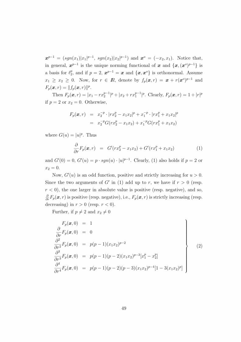
xp−1 = (sgn(x1)|x1|p−1, sgn(x2)|x2|p−1) and xo = (−x2, x1). Notice that,

in general, xp−1 is the unique norming functional of x and x, (xo)p−1 is

a basis for `p2, and if p = 2, xp−1 = x and x, xo is orthonormal. Assume

x1 ≥ x2 ≥ 0. Now, for r ∈ IR, denote by fp(x, r) = x + r(xo)p−1 and

Fp(x, r) = ‖fp(x, r)‖p.

Then Fp(x, r) = |x1− rxp−12 |p + |x2 + rxp−1

1 |p. Clearly, Fp(x, r) = 1 + |r|p

if p = 2 or x2 = 0. Otherwise,

Fp(x, r) = x−p2 · |rxp

2 − x1x2|p + x−p1 · |rxp

1 + x1x2|p

= x−p2 G(rxp

2 − x1x2) + x−p1 G(rxp

1 + x1x2)

where G(u) = |u|p. Thus

∂

∂rFp(x, r) = G′(rxp

2 − x1x2) + G′(rxp1 + x1x2) (1)

and G′(0) = 0, G′(u) = p · sgn(u) · |u|p−1. Clearly, (1) also holds if p = 2 or

x2 = 0.

Now, G′(u) is an odd function, positive and strictly increasing for u > 0.

Since the two arguments of G′ in (1) add up to r, we have if r > 0 (resp.

r < 0), the one larger in absolute value is positive (resp. negative), and so,∂∂r

Fp(x, r) is positive (resp. negative), i.e., Fp(x, r) is strictly increasing (resp.

decreasing) in r > 0 (resp. r < 0).

Further, if p 6= 2 and x2 6= 0

Fp(x, 0) = 1∂

∂rFp(x, 0) = 0

∂2

∂r2Fp(x, 0) = p(p− 1)(x1x2)

p−2

∂3

∂r3Fp(x, 0) = p(p− 1)(p− 2)(x1x2)

p−3[xp1 − xp

2]

∂4

∂r4Fp(x, 0) = p(p− 1)(p− 2)(p− 3)(x1x2)

p−4[1− 3(x1x2)p]

(2)

49

and so, if 1 < q < ∞, for Hpq(x, r) = [Fp(x, r)]q/p, we have,

Hpq(x, 0) = 1∂

∂rHpq(x, 0) = 0

∂2

∂r2Hpq(x, 0) = q(p− 1)(x1x2)

p−2

∂3

∂r3Hpq(x, 0) = q(p− 1)(p− 2)(x1x2)

p−3[xp1 − xp

2]

∂4

∂r4Hpq(x, 0) = q(p− 1)(x1x2)

p−4[(p− 2)(p− 3)

− 3(x1x2)p(p− 2)(p− 3) + (p− q)(p− 1)]

(3)

Now, let 1 < p, q < ∞. Let T : `p2 −→ `q

2, ‖T‖ = 1. Then there exists

x = (x1, x2) ∈ `p2 such that ‖x‖ = 1 = ‖Tx‖. Let Tx = y = (y1, y2).

Let Ixy = T : ‖T‖ ≤ 1, Tx = y. Then for any T ∈ Ixy, (T − xp−1 ⊗ y)

annihilates x and so is of rank ≤ 1, whence (T − xp−1 ⊗ y) = xo ⊗ u, for

some u ∈ `p2. Further, T ∗(yq−1) = xp−1, that is (T ∗ − y ⊗ xp−1) annihilates

yq−1, whence (T ∗− y⊗xp−1) = (yo)q−1⊗ v, for some v ∈ `q2. Combining, T

must be of the form

Ts = xp−1 ⊗ y + sxo ⊗ (yo)q−1, for some s ∈ IR

In other words, Ixy = Ts : s ∈ IR, ‖Ts‖ ≤ 1.As in [34], pre- or post-multiplying by diag(sgn(x1), sgn(x2)),

diag(sgn(y1), sgn(y2)) and permutation matrices, if necessary — each of

which is an isometry — we may assume x1 ≥ x2 ≥ 0, y1 ≥ y2 ≥ 0.

Now, Ts(fp(x, r)) = fq(y, rs), and it follows from the above discussion

that for any r 6= 0, ‖Ts(fp(x, r))‖q = Fq(y, rs) is strictly increasing in s ≥ 0

and strictly decreasing in s ≤ 0, and Fq(y, rs) is unbounded in s. Now, if

r 6= 0,

Fq(y, 0) = 1 = [Fp(x, 0)]q/p < [Fp(x, r)]q/p

so, there exists unique s+(x, y, r) > 0 and unique s−(x, y, r) < 0 such that

Fq(y, rs±) = [Fp(x, r)]q/p (4)

And the quantity on the LHS becomes smaller or larger than the one in the

RHS according as |s| gets smaller or larger. Evidently, such s± also exist for

50

(xo)p−1, which we denote by fp(x,∞). In fact, in this case, |s±(x, y,∞)| =‖(xo)p−1‖/‖(yo)q−1‖. Notice that for fixed x, y, s± is a continuous function

of r 6= 0 and elementary examples show that limr→0 s±(x, y, r) may not even

exist. Let

s∗+(x, y) = infs+(x, y, r) : r 6= 0 s∗∗+ (x, y) = lim infr→0

s+(x, y, r)

s∗−(x, y) = sups−(x, y, r) : r 6= 0 s∗∗− (x, y) = lim supr→0

s−(x, y, r)

where lim infr→0 s+(x, y, r) = supε>0 infs+(x, y, r) : |r| < ε and

lim supr→0 s−(x, y, r) = infε>0 sups−(x, y, r) : |r| < ε. Clearly, s∗∗− ≤s∗− ≤ 0 ≤ s∗+ ≤ s∗∗+ and Ts ∈ Ixy if and only if s∗− ≤ s ≤ s∗+, i.e., Ts∗±

are

end points of Ixy and hence are extreme. Also note that if Jxy = s : Ts is

contractive in a neighbourhood of x, then s∗∗− = inf Jxy and s∗∗+ = sup Jxy.

Now, either s∗± equals s±(x, y, r) for some r 6= 0 (including r = ∞), in

which case s∗± 6= 0 and Ts∗±attain their norm on two linearly independent

vectors, or s∗± = s∗∗± , in which case |s∗∗± | < ∞, s∗∗± ∈ Jxy, in fact, Ts∗∗±∈ Ixy.

Note that T attains its norm on two linearly independent vectors if and

only if T ∗ attains its norm on two linearly independent vectors. Moreover,

any such T is exposed, and hence strongly exposed.

Fix x, y.

Case(I) : (i) p = 2 and either q = 2 or y2 = 0; (ii) q = 2 and either p = 2

or x2 = 0; (iii) p 6= 2 6= q and x2 = 0 = y2.

Ts is a contraction ⇐⇒ Fq(y, rs) ≤ [Fp(x, r)]q/p for all r

⇐⇒ 1 + |rs|q ≤ [1 + |r|p]q/p for all r

⇐⇒ |s|q ≤ [1 + |r|p]q/p − 1

|r|qfor all r 6= 0

Note that the RHS ≡ 1 if p = q and is strictly decreasing (resp. increasing)

in |r| for q > p (resp. q < p).

So, if p = q, s± ≡ ±1, and hence, s∗± = s∗∗± = ±1 and Ts∗±are isometries.

And, if p 6= q, the infimum of the RHS over r 6= 0 yields

|s∗±|q =

1 if q > p

0 if q < p

51

So, if q < p, s∗± = 0, hence Ixy = T0, and

T0 =

x⊗ e1 if p = 2 > q

e∗1 ⊗ y if p > q = 2

e∗1 ⊗ e1 if p > q, p 6= 2 6= q

is an extreme contraction which attains its norm at precisely one point.

And if q > p, s∗± = s±(∞) = ±1 with T±1 attaining its norm at both x

and (xo)p−1. It is interesting to note that if p 6= 2 6= q, T1 in this case is the

identity operator.

In each of the following cases our basic aim is to find extreme contractions

that do not attain their norm on two linearly independent vectors. Then nec-

essarily s∗± = s∗∗± . So, we first assume |s∗∗± | < ∞. If we reach a contradiction,

we conclude that s∗∗± = ±∞, whence s∗± 6= s∗∗± and Ts∗±is not of the desired

type. Otherwise, we check whether s∗∗± ∈ Jxy. If it does not, we are again

done. And if it does, we further check whether Ts∗∗±gives a contraction. If

it does not, we are done, and if it does, we get an extreme contraction. We

then check whether it attains its norm in any direction other than that of x

and only if it does not, we get an extreme contraction of the desired type.

This is exemplified in the analysis below.

To calculate s∗∗± , let rn be a sequence of real numbers such that rn → 0

and s±(rn) → s∗∗± . Since |s∗∗± | < ∞, s±(rn) is a bounded sequence. Now,

by (4),

Fq(y, rns±(rn)) = [Fp(x, rn)]q/p (5)

Case (II) : q 6= 2, y2 > 0 and either p = 2 or x2 = 0.

In this case, subtracting 1 from both side of (5), dividing by r2n and

taking limit as n −→ ∞, we get by L’Hospital’s rule and (2) that LHS −→12q(q − 1)s2(y1y2)

q−2, where s = s∗∗± and

RHS −→

0 if p > 2

∞ if p < 2q

2if p = 2

So, if p < 2, we have a contradiction, whence s∗∗± = ±∞, so that Ts∗±is not

of the desired type, and if p > 2, s∗± = s∗∗± = 0, Ixy = T0 and T0 = e∗1 ⊗ y

is extreme, and clearly of the desired type.

52

If p = 2, we have

s2(q − 1)(y1y2)q−2 = 1 (6)

Now, if the s given by (6) belongs to Jxy, we must have

Fq(y, rs) ≤ [Fp(x, r)]q/p for all small r 6= 0 (7)

By (2), the Taylor expansion of the LHS above around r = 0 is given by

1 +1

2!q(q − 1)r2s2(y1y2)

q−2 +1

3!q(q − 1)(q − 2)r3s3(y1y2)

q−3[yq1 − yq

2]

+1

4!q(q − 1)(q − 2)(q − 3)r4s4(y1y2)

q−4[1− 3(y1y2)q] + · · ·

while that of the RHS is given by

1 +1

2qr2 +

1

8q(q − 2)r4 + · · ·

Comparing the two, we see that the coefficients of 1, r and r2 on both sides

are equal, whence the inequality (7) for small r implies the corresponding

inequality for the coefficient of r3 on both sides, which, for r > 0 and r < 0,

leads to the following equality :

1

6s3q(q − 1)(q − 2)(y1y2)

q−3(yq1 − yq

2) = 0 (8)

Combining equations (6) and (8), we have yq1 = yq

2 = 1/2, s2 =1

(q−1)4(q−2)/q. But again the equality in (8) forces the inequality of the coef-

ficient of r4, i.e.,

1

8q(q − 2) ≥ 1

24s4q(q − 1)(q − 2)(q − 3)(y1y2)

q−4[1− 3(y1y2)q]

or 3(q − 2) ≥ (q − 2)(q − 3)

(q − 1)

Now for q < 2, this leads to a contradiction, so that s∗∗± 6∈ Jxy. And

for q > 2, by [28, Proposition 1], Ts with these parameters is a contraction

that attains its norm only in the direction of x. So for q > 2, Ts with these

parameters is of the desired type and for q < 2, s∗± 6= s∗∗± , so that Ts∗±is not

of the desired type.

53

Case (III) : p 6= 2, x2 > 0 and either q = 2 or y2 = 0.

This is the situation dual to case (II) and hence, if q < 2, s∗± = s∗∗± = 0,

Ixy = T0 and T0 = xp−1 ⊗ e1 is extreme and of the desired type; if q > 2,

s∗± 6= s∗∗± , so that Ts∗±is not of the desired type, and if q = 2, then for p < 2,

s∗± = s∗∗± = ±√

(p− 1)2(2−p)/p, x1 = x2 = (1/2)1/p, Ts∗±is of the desired type,

and for p > 2, Ts∗±is not of the desired type.

Case(IV) : p 6= 2 6= q and x2 > 0, y2 > 0.

In this case too, subtracting 1 from both side of (5), dividing by r2n and

taking limit as n →∞, we get by (2) and (3)

(q − 1)(y1y2)q−2s2 = (p− 1)(x1x2)

p−2 (9)

where s = s∗∗± . Now,

s = ±[(p− 1)(x1x2)

p−2

(q − 1)(y1y2)q−2

]1/2

= ±[(p− 1)(x1x2)

p

(q − 1)(y1y2)q

]1/2

· y1y2

x1x2

Put α =

[(p− 1)(x1x2)

p

(q − 1)(y1y2)q

]1/2

, then s = ±αy1y2

x1x2

, whence

Ts = xp−1 ⊗ y + sxo ⊗ (yo)q−1

=

xp−11 y1 xp−1

2 y1

xp−11 y2 xp−1

2 y2

± αy1y2

x1x2

yq−12 x2 −yq−1

2 x1

−yq−11 x2 yq−1

1 x1

=

xp

1y1

x1

xp2y1

x2xp

1y2

x1

xp2y2

x2

± α

y1y

q2

x1

−y1yq2

x2

−y2yq1

x1

y2yq1

x2

=

y1

x1

(xp1 ± αyq

2)y1

x2

(xp2 ∓ αyq

2)

y2

x1

(xp1 ∓ αyq

1)y2

x2

(xp2 ± αyq

1)

(10)

To continue, in this case, by (2), the Taylor expansion of the LHS of (7)

around r = 0 is given by

1 +1

2!q(q − 1)r2s2(y1y2)

q−2 +1

3!q(q − 1)(q − 2)r3s3(y1y2)

q−3[yq1 − yq

2]

+1

4!q(q − 1)(q − 2)(q − 3)r4s4(y1y2)

q−4[1− 3(y1y2)q] + · · ·

54

while by (3), that of the RHS is given by

1 +1

2!q(p− 1)r2(x1x2)

p−2 +1

3!q(p− 1)(p− 2)r3(x1x2)

p−3[xp1 − xp

2]

+1

4!q(p− 1)r4(x1x2)

p−4[(p− 2)(p− 3)− 3(x1x2)p ·

(p− 2)(p− 3) + (p− q)(p− 1)] + · · ·

So, if s ∈ Jxy, by similar arguments, we must have

s3(q − 1)(q − 2)(y1y2)q−3(yq

1 − yq2) = (p− 1)(p− 2)(x1x2)

p−3(xp1 − xp

2) (11)

and

s4(q − 1)(q − 2)(q − 3)(y1y2)q−4[1− 3(y1y2)

q] ≤ (p− 1)(x1x2)p−4 ·

[(p− 2)(p− 3)1− 3(x1x2)p − 3(p− q)(p− 1)(x1x2)

p] (12)

Eliminating s from (9) and (11) and using the fact that x, y are unit

vectors, we get

(q − 2)2

(q − 1)

[1

(y1y2)q− 4

]=

(p− 2)2

(p− 1)

[1

(x1x2)p− 4

](13)

Also, dividing (12) by the square of (9), we get

(q − 2)(q − 3)

(q − 1)

[1

(y1y2)q− 3

]≤ (p− 2)(p− 3)

(p− 1)

[1

(x1x2)p− 3

]− 3(p− q) (14)

Notice that if p = q, we get from (13) that xi = yi, i = 1, 2, whence from

(9), s = ±1, and from (11), y1 = y2 = x1 = x2 for s = −1. Also, (14) is

consistent with (13) and equality holds. Now in (10), α = 1, and so,

T1 =

1 0

0 1

and T−1 =

0 1

1 0

and hence, clearly, are isometries.

Now, let p 6= q. From (13) and (14), writing1

(x1x2)p= A, we get

(p− 2)2(q − 3)

(q − 2)(p− 1)(A− 4) +

(q − 2)(q − 3)

(q − 1)≤ (p− 2)(p− 3)

(p− 1)(A− 3)− 3(p− q)

55

or [(p− 2)2(q − 3)

(q − 2)(p− 1)− (p− 2)(p− 3)

(p− 1)

]· A

≤ 4(p− 2)2(q − 3)

(q − 2)(p− 1)− 3(p− 2)(p− 3)

(p− 1)− (q − 2)(q − 3)

(q − 1)− 3(p− q)

=

[3(p− 2)2(q − 3)

(q − 2)(p− 1)− 3(p− 2)(p− 3)

(p− 1)

]+

[(p− 2)2(q − 3)

(q − 2)(p− 1)

− (q − 2)(q − 3)

(q − 1)

]− 3(p− q)

Simplifying we get

(q − p)(p− 2)

(p− 1)(q − 2)· A ≤ 2q(q − p)(pq − p− q)

(p− 1)(q − 1)(q − 2)

So, if (a) 1 < q < 2 < p < ∞, or, (b) 1 < p < q < 2, or, (c) 2 < p < q < ∞,

we have

A ≤ 2q(pq − p− q)

(p− 2)(q − 1)i.e., A− 4 ≤ 2(q − 2)(pq − p− q + 2)

(p− 2)(q − 1)(15)

And if (d) 1 < p < 2 < q < ∞, or, (e) 1 < q < p < 2, or, (f) 2 < q < p < ∞,

we have

A ≥ 2q(pq − p− q)

(p− 2)(q − 1)i.e., A− 4 ≥ 2(q − 2)(pq − p− q + 2)

(p− 2)(q − 1)(16)

Now, (x1x2)p = 1/A and xp

1 + xp2 = 1, so 0 < 1/A ≤ 1/4, i.e., A ≥ 4 or

A− 4 ≥ 0.

But since (pq − p − q + 2) = (p − 1)(q − 1) + 1 is always positive for

1 < p, q < ∞, if 1 < q < 2 < p < ∞, i.e., in case (a) above, we reach a

contradiction at this point, whence Ts∗±is not of the desired type.

Summarising the results so far, we have the following

Theorem 4.9 For 1 < p, q < ∞, an operator T : `p2 −→ `q

2 with ‖T‖ = 1 is

an extreme contraction

(i) [26] for p = q = 2, if and only if T is an isometry.

(ii) [28] for p = 2 6= q, if and only if T satisfies one of the following

(a) T attains its norm on two linearly independent vectors.

56

(b) T is of the form

T =

x⊗ ei if q < 2

x⊗ y + sxo ⊗ (yo)q−1 if q > 2

where x is any unit vector and, in the second case, |yi|q = 12

and

s = ± 1√(q−1)

2(q−2)/q.

(iii) [28] for p 6= 2 = q, if and only if T satisfies one of the following

(a) T attains its norm on two linearly independent vectors.

(b) T is of the form

T =

ei ⊗ y if p > 2

xp−1 ⊗ y + sxo ⊗ yo if p < 2

where y is any unit vector and, in the second case, |xi|p = 12

and

s = ±√

(p− 1)2(2−p)/p.

(iv) [25] for p = q, if and only if T satisfies one of the following

(a) T attains its norm on two linearly independent vectors.

(b) T is of the form

T =

e∗i ⊗ y if p > 2, y1y2 6= 0

xp−1 ⊗ ej if p < 2, x1x2 6= 0

(v) for 1 < q < 2 < p < ∞, if and only if T satisfies one of the following

(a) T attains its norm on two linearly independent vectors.

(b) T = xp−1 ⊗ y with x, y unit vectors and x1x2y1y2 = 0.

Remark : In the discussion preceding Theorem 4.9, the conditions (b)

and (e) are dual to (c) and (f) respectively. And in the cases (b) and (c), the

inequality (15) implies

1

2≤ xp

1 ≤1

2

1 +

√√√√(q − 2)(pq − p− q + 2)

q(pq − p− q)

(17)

while in cases (e) and (f), the inequality (16) implies

1

2

1 +

√√√√(q − 2)(pq − p− q + 2)

q(pq − p− q)

≤ xp1 < 1 (18)

57

Now, in cases (b), (c), (e) and (f), we have from (11) that for s < 0, both

sides of (11) must be 0, i.e., we must have xp1 = xp

2 = 1/2 = yq1 = yq

2. But

then in cases (e) and (f), we have a contradiction. So, in these two cases, s∗−

gives extreme contractions not of the desired type.

Also in case (d), (16) is always satisfied and (11) implies that for s > 0,

xp1 = xp

2 = 1/2 = yq1 = yq

2. Now combining Propositions 1 and 2 of [28], we

see easily that for xp1 = xp

2 = 1/2 = yq1 = yq

2 for both s > 0 and s < 0, we

have a contraction that attains its norm only in the direction of x, i.e., we

get extreme contractions of the desired type.

Thus, we are left with the following cases unsolved :

(1) Case (b) with x1 satisfying (17) for s > 0 and xp1 = 1/2 for s < 0 with

y1 given by (13).

(2) Case (e) with x1 satisfying (18) for s > 0 with y1 given by (13).

(3) Case (d) with xp1 > 1/2 and s < 0 with y1 given by (13).

Notice that for 1p+ 1

q= 1, (p < 2), (13) gives xp

i = yqi , i = 1, 2, whence in

this case, Ts — as given by (10) — has a comparatively simpler form.

We proceed now to find the closure of the extreme contractions in the

cases described in Theorem 4.9. In case (i), the set of extreme contractions

is clearly closed. Also, in the cases (ii), (iii) and (v), the set of operators

of the form (b) is clearly closed. And in case (iv), the closure of the set of

operators of the form (b) contains only the operators ei ⊗ ej, i, j = 1, 2 in

addition.

Let us consider the set of operators of the type (a) in cases (ii), (iv) and

(v). Let Tn be a sequence of operators of the type (a). Let Tn −→ T in

operator norm. Let xn = (xn1, xn2) be such that ‖xn‖ = 1 = ‖Tnxn‖. Let

Tnxn = yn = (yn1, yn2). Then Tn is of the form

Tn = xp−1n ⊗ yn + s∗±(xn, yn)xo

n ⊗ (yon)q−1

where s∗±(xn, yn) is as in our earlier discussion. For notational simplicity,

write s∗±(xn, yn) = ±sn. Passing to a subsequence, if necessary, assume

xn → x = (x1, x2), yn → y = (y1, y2) (by compactness of the unit balls of

`p2 and `q

2), and all the sn’s have the same sign, without loss of generality,

positive.

58

Clearly, ‖T‖ = 1 and Tx = y, whence T is of the form

T = xp−1 ⊗ y + sxo ⊗ (yo)q−1

Also, as Tn −→ T , sn = ‖Tn − xp−1n ⊗ yn‖/‖xo

n‖ · ‖(yon)q−1‖ −→ ‖T −

xp−1 ⊗ y‖/‖xo‖ · ‖(yo)q−1‖, i.e., sn is convergent. Clearly, sn → s.

Now, since Tn is of the type (a), there exists zn = xn + rn(xon)p−1 with

rn 6= 0 ∈ IR such that ‖Tnzn‖ = ‖zn‖. Again we may assume all rn’s are

of the same sign, in particular positive and rn → r, where 0 ≤ r ≤ ∞. If

0 < r < ∞, zn → z = x+r(xo)p−1 and ‖Tz‖ = ‖z‖, i.e., T is also of the type

(a). Also, if rn →∞, let un = zn/‖zn‖. Then un → u = (xo)p−1/‖(xo)p−1‖and ‖Tu‖ = 1, so that T again is of the type (a).

Now, suppose rn → 0. Then from ‖Tnzn‖ = ‖zn‖ we have

Fq(yn, rnsn)− [Fp(xn, rn)]q/p = 0 (19)

For (ii), if p = 2 and q < 2, since Tn is of type (a), we have yn1yn2 6= 0 for

all n. And if q > 2, we have two possibilities; either there is a subsequence

for which yn1yn2 = 0, or, eventually yn1yn2 6= 0. In the first case, we restrict

ourselves only to that subsequence, and we have, by case(I), sn = 1 for all n,

whence s = 1. Also, y1y2 = 0. So, T = x ⊗ ei + xo ⊗ ej (i 6= j), and it is

clear that T is of type (a) (see case (I)). And in the second case, we assume

yn1yn2 6= 0 for all n. Then dividing (19) by r2n and taking limit as n → ∞,

we get by L’Hospital’s rule

(q − 1)s2(y1y2)q−2 − 1 = 0 (20)

If q > 2, for y1y2 = 0, this leads to a contradiction, whence either rn 6→ 0

(in which case we get an operator of type(a)), or y1y2 6= 0. In the latter

case, (6) and (20) coincides, i.e., we have s = s∗∗+ (x, y). Now, our analysis in

case (II) shows that only for yq1 = yq

2 = 1/2, s∗∗+ gives a contraction (which is

an extreme contraction of type (b)). And in every other case, we run into a

contradiction, i.e., we must have rn 6→ 0.

And if q < 2, for y1y2 = 0, (20) makes sense only if s = 0. In that case,

T = x ⊗ ei, which, by case (I), is an extreme contraction of the type (b).

59

And for y1y2 6= 0, we again have s = s∗∗+ (x, y) and our analysis in case (II)

shows that this case always leads to a contradiction, whence rn 6→ 0.

So, in both the cases, the closure of the set of operators of the type (a)

contains at most operators of type (b), and therefore, the set of extreme

contractions is closed.

Since case (iii) is just the dual of case (ii), the set of extreme contractions,

in this case too, is closed.

In (iv), i.e., if p = q, by duality, it suffices to consider p > 2. Since Tn

is of type (a), we have three possibilities; either there is a subsequence for

which both xn1xn2 = 0 and yn1yn2 = 0, or, there is a subsequence for which

xn1xn2 6= 0 and yn1yn2 = 0, or, eventually both xn1xn2 6= 0 and yn1yn2 6= 0.

In the first case, we again restrict ourselves only to that subsequence,

and we have, by case(I), sn = 1 for all n, whence s = 1. Also, x1x2 = 0 and

y1y2 = 0. Now again by case (I), T is of type (a).

In the second and the third case, dividing (19) by r2n and taking limit —

through a subsequence if necessary — as n →∞, we get in the second case

(x1x2)p−2 = 0

and in the third case

(y1y2)p−2s2 = (x1x2)

p−2

So, in the second case, y1y2 = 0, and we have a contradiction unless

x1x2 = 0. And in that case, T is of the form diag(1, s) upto isometric factors

of signum or permutation matrices. Now, T is a contraction for −1 ≤ s ≤ 1

and is extreme (in fact, an isometry) only for s = ±1.

In the third case, if x1x2 = 0, we get a contradiction unless y1y2 = 0 or

s = 0. If y1y2 6= 0, s = 0 = s∗±(x, y), whence T is extreme. And if y1y2 = 0,

we get the conclusions as in the second case. If x1x2 6= 0, y1y2 = 0 leads to a

contradiction (and therefore, rn 6→ 0), and if y1y2 6= 0, s = s∗∗+ (x, y), so that

T is an isometry and hence is of type (a).

Thus, in case (iv), the closure of the operators of type (a), and so the

closure of extreme contractions, can have at most operators of the form

diag(1, s), |s| < 1, upto isometric factors of signum or permutation matrices

60

as additional elements. However, we do not have precise description of the

closure.

In case (v), i.e., if 1 < q < 2 < p < ∞, since Tn is of type (a), we must

have xn1xn2yn1yn2 6= 0 for all n. And a similar argument leads to

s2(q − 1)(y1y2)q−2 = (p− 1)(x1x2)

p−2

If x1x2 6= 0 the only situation that does not lead to any contradiction —

either immediate or to the fact that T is a contraction — is both y1y2 = 0

and s = 0. And in that case, s = 0 = s∗±(x, y), so that T is extreme.

And if x1x2 = 0, we must have s = 0, in which case, by cases (I) and (II),

s = 0 = s∗±(x, y) and T is extreme. Thus in this case too, the set of extreme

contractions is closed.

Theorem 4.10 In each of the following cases of 1 < p, q < ∞, `p2 ⊗π `q

2

lacks the MIP :

(i) p and q are conjugate exponents, i.e., 1p

+ 1q

= 1.

(ii) Either p or q is equal to 2.

(iii) 2 < p, q < ∞.

Proof : The dual of `p2 ⊗π `q

2 is L(`p2, `

q′

2 ), where 1q

+ 1q′

= 1 and the closure

of extreme contractions in each of the above cases does not contain norm

1 operators of the form xp−1 ⊗ y, where x and y are unit vectors with

x1x2y1y2 6= 0.

Remark : The fact that operators of the above form do not belong to

the closure of extreme contractions in any of these cases seems to suggest

that this is a general phenomenon. It is possible that this is happens in

higher dimensions as well. Can one give a proof of this without precisely

characterising the extreme contractions ? What seems to be required is a

more tractable necessary condition for extremality, or, for belonging to the

closure of extreme contractions.

61

Chapter 5

Exposed Points of Continuityand Strongly Exposed Points

In this chapter, we make the following change in our notations. For a Banach

space X and A ⊆ X, by Ao, the polar of A, we mean Ao = f ∈ X∗ : f(x) ≤ 1

for all x ∈ A (i.e., we do not take the absolute value of f(x)).

If K is a closed bounded convex set in X and f ∈ X∗, we will say that

f ∈ X∗ supports K at xo ∈ K if f(xo) = M(K, f) and we let S(K, xo) =

f ∈ X∗ : f(xo) = M(K, f). Note that S(K, xo) is a w*-closed convex cone

with vertex 0. We may sometimes abbreviate S(K, xo) by S(xo) when there

is no scope of confusion.

Call xo ∈ K a relatively exposed point of K if for each x ∈ K \ xo there

exists fx ∈ S(K, xo) such that fx(x) < fx(xo). Call xo a vertex of K if for

each x ∈ X \ xo there exists fx ∈ S(K,xo) such that fx(x) 6= fx(xo), or, in

other words, S(K, xo) separates points of X. We can also define w*-relatively

exposed points or w*-vertices similarly. Obviously, a (w*-) vertex is (w*-)

relatively exposed.

5.1. The Counterexample

Let δn : n ≥ 1 denote the canonical basis of `1. Recall that `1 as a dual

space has a w*-topology induced on it. Let

K = cow∗ [ 1

nδ1 + δn : n ≥ 2 ∪ 1

n2δ1 −

1

nδn : n ≥ 2]

From Milman’s Theorem (see [43, p 9]) and the metrizable version of Cho-

quet’s Theorem ([1] or [43]), it follows that x ∈ K if and only if x is of the

62

form

x =∑n≥2

αn(1

nδ1 + δn) +

∑n≥2

βn(1

n2δ1 −

1

nδn)

with αn, βn ≥ 0 and∑

n≥2(αn+βn) ≤ 1 (see [7, Example 3.2.5] for the details

in a similar situation). Observe that (−1, 0, 0, . . .) ∈ co ⊆ `∞ = (`1)∗ exposes

0 = (0, 0, . . .) ∈ K. If f = (an) ∈ `∞ supports K at 0, then 1na1 ± an ≤ 0 for

n ≥ 2, from which it follows that a1 ≤ 0 and |an| ≤ 1n|a1|, (n ≥ 2) and we

see therefore that (an) ∈ co. Since f( 1m

δ1 + δm) = 1m

a1 + am → 0 as m →∞,

S(K, f, α) = y ∈ K : f(y) > −α contains 1m

δ1 + δm for all sufficiently

large m, whence diam[S(K, f, α)] ≥ ‖ 1m

δ1 + δm‖ > 1, showing that 0 is not

strongly exposed.

Next, for m ≥ 2, let fm = (−1,− 1m2 , . . . ,− 1

m2 ,− 1m

,− 1m

, . . .) ∈ `∞ where

the mth coordinate onwards of fm has the value − 1m

and consider the slice

Sm = y ∈ K : fm(y) > − 1m3 determined by fm. Clearly, 0 ∈ Sm and if

x =∑n≥2

αn(1

nδ1 + δn) +

∑n≥2

βn(1

n2δ1 −

1

nδn) ∈ Sm

we must have

− 1

m3< −

m−1∑n=2

αn ·m2 + n

m2n−∑n≥m

αn ·m + n

mn−

m−1∑n=2

βn ·m2 − n

m2n2+∑n≥m

βn ·n−m

n2m

whence it follows that

1

m2>

m−1∑n=2

αn ·n + 1

n· m2 + n

m(n + 1)+∑n≥m

αn ·n + 1

n· m + n

n + 1

+m−1∑n=2

βn ·n + 1

n2· m2 − n

m(n + 1)−∑n≥m

βn ·n−m

n2

≥m−1∑n=2

αn ·n + 1

n+∑n≥m

αn ·n + 1

n+

m− 1

m + 1

m−1∑n=2

βn ·n + 1

n2− 1

4m

on using successively the following easily verified inequalities :

(i) for all m ≥ 1 and n ≤ m,m2 + n

m(n + 1)≥ 1.

(ii) for all m ≥ 1,m + n

n + 1≥ 1.

(iii) for all n ≤ m,m2 − n

m(n + 1)≥ m− 1

m + 1, since

m2 − n

m(n + 1)is decreasing in n.

63

(iv) for all m, n ≥ 1,n−m

n2≤ 1

4m.

Thus,

m + 1

m− 1· m + 4

4m2≥ m + 1

m− 1

∑n≥2

αn ·n + 1

n+

m−1∑n=2

βn ·n + 1

n2

≥∑n≥2

αn ·n + 1

n+

m−1∑n=2

βn ·n + 1

n2

Now,

‖x‖ =∑n≥2

(αn

n+

βn

n2

)+∑n≥2

∣∣∣∣∣αn −βn

n

∣∣∣∣∣ ≤ ∑n≥2

αn ·n + 1

n+∑n≥2

βn ·n + 1

n2

≤ (m + 1)(m + 4)

4m2(m− 1)+∑n≥m

βn ·n + 1

n2≤ (m + 1)(m + 4)

4m2(m− 1)+

m + 1

m2

=5(m + 1)

4m(m− 1)≤ 15

4mfor all m ≥ 2.

Hence, diam(Sm) ≤ 15/2m → 0 as m → ∞ and we conclude that 0 is a

denting point of K.

Remarks : 1. Let Fo be a w*-cluster point of 1nδ1 + δn : n ≥ 2 in

K. Then Fo 6= 0 since Fo(fo) = 1 where fo = (1, 1, . . . , 1, . . .) ∈ `∞. As

S(0) ⊆ co, we must have Fo ∈ ∩ker(f) : f ∈ S(0) and hence 0 is not w*-

relatively exposed in K. This observation proved useful in the formulation

(d) of Theorem 5.3 in the next section.

2. Since S(0) ⊆ co, one in fact has S(0) = (an) ∈ co : a1 ≤ 0 and

|an| ≤ 1n|a1|, n ≥ 2. It is now easy to see that S(0) separates points of `1,

i.e., 0 is a vertex of K.

5.2. A Characterisation Theorem

We need the following lemma :

Lemma 5.1 Let K be a compact convex set in a locally convex space E.

Then

(a) xo ∈ K is exposed by f ∈ E∗ if and only if S(K, f, α) : α > 0forms a local base for the relative topology on K at xo.

64

(b) A relatively exposed point xo ∈ K is exposed if and only if xo is a

Gδ point.

Proof : (a) The sufficiency is obvious and the necessity follows from the

compactness of K.

(b) [We follow [1, p 119]] If xo is exposed by f ∈ E∗, then xo =

∩n≥1S(K, f, 1n) is clearly Gδ.

Conversely, let xo be relatively exposed and xo = ∩n≥1Wn, where Wn is

open in K. Now, an easy compactness argument shows that for any compact

subset F of K with xo 6∈ F , there exists f ∈ E∗ such that f ∈ S(xo) and

f(y) < f(xo) for all y ∈ F .

Since for all n ≥ 1, Wn is open in K, by the above argument, there exists

fn ∈ S(xo) such that fn(y) < fn(xo) for all y ∈ K \Wn. It is now esay to

show that f =∑

n≥112n fn exposes xo.

Theorem 5.2 Let K be a w*-compact convex set in a dual Banach space X∗

and x∗o ∈ K be a w*-PC. The following are equivalent :

(a) x∗o ∈ K is w*-strongly exposed.

(b) x∗o ∈ K is w*-exposed.

(c) x∗o ∈ K is w*-relatively exposed.

Proof : Follows from Lemma 5.1 and the fact that a w*-PC is a w*-Gδ

point.

Theorem 5.3 Let K be a closed bounded convex set in a Banach space X

and xo ∈ K be a PC. The following are equivalent :

(a) xo ∈ K is strongly exposed.

(b) xo ∈ K is w*-strongly exposed.

(c) xo ∈ K is w*-exposed.

(d) xo ∈ K is w*-relatively exposed.

(e) X∗/sp(S(xo)) = π[(K − xo)o] where π : X∗ −→ X∗/sp(S(xo)) is the

quotient map and the closure is with respect to the norm topology.

65

Proof : (a) ⇐⇒ (b) is immediate, while (b) ⇐⇒ (c) ⇐⇒ (d) follows from

Theorem 5.2 and Lemma 1.4.

(d) ⇐⇒ (e) : Using definitions, simple separation arguments and polar

calculations a la the Bipolar Theorem, each of the statement below is easily

seen to be equivalent to the next :

(1) xo is w*-relatively exposed in K.

(2) 0 is w*-relatively exposed in K1, where K1 = K − xo.

(3) K1 ∩ [∩ker(f) : f ∈ S(xo)] = 0.

(4) Koo1 ∩ [sp(S(xo))]

o = 0, · · · (∗)(since ∩ker(f) : f ∈ S(xo) = [sp(S(xo))]

⊥ = [sp(S(xo))]o and K1 =

Koo1 )

(5) [Ko1 ∪ sp(S(xo))]

o = 0.

(6) co[Ko1 ∪ sp(S(xo))] = X∗.

This last condition implies that [sp(S(xo)) + Ko1 ] = X∗ which in turn

means that

X∗/sp(S(xo)) = π(Ko1). · · · (∗∗)

Conversely, suppose that (∗∗) holds and that φ ∈ Koo1 ∩ [sp(S(xo))]

o. We

get immediately

(a) φ ∈ [sp(S(xo))]o = [X∗/sp(S(xo))]

∗, and

(b) M(Ko1 , φ) ≤ 1.

But (a) and (b) together give M(π(Ko1), φ) ≤ 1 and using (∗∗), we see that

φ = 0, thus (∗) holds.

Corollary 5.3.1 If K is weakly compact then xo ∈ K is strongly exposed if

and only if xo is exposed and PC.

Proof : Follows immediately from Theorem 5.2 or from Theorem 5.3, once

we observe that if K is weakly compact, K = K and that xo ∈ K is w*-

exposed if xo ∈ K is exposed.

Corollary 5.3.2 (a) Let K be a closed bounded convex set in a Banach space

X. xo ∈ K is strongly exposed if and only if xo is contained in slices of K

determined by functionals from S(K,xo) of arbitrarily small diameter.

66

(b) Let K be a w*-compact convex set in a dual Banach space X∗. x∗o ∈K is w*-strongly exposed if and only if x∗o is contained in w*-slices of K

determined by functionals from S(K, x∗o) ∩X of arbitrarily small diameter.

Remarks : 1. Note that the proof of (d) ⇐⇒ (e) in Theorem 5.3 does

not use the fact that xo is a PC.

2. If xo is a PC and xo ∈ K is a w*-vertex, or equivalently, xo is a PC and

sp(S(xo)) is dense in X∗, it follows from Theorem 5.3, that xo is strongly

exposed. But, if xo ∈ K is a strongly exposed point with a unique (upto

scalar multiples) exposing functional — this happens for instance for any

boundary point of the unit ball of the Euclidean space IR2 — then sp(S(xo))

is 1-dimensional and thus X∗ 6= sp(S(xo)), i.e., this condition is, in general,

not necessary. And since 0 in our example is a vertex (see Remark 2), the

weaker condition that xo is a PC and xo ∈ K is a vertex is no longer sufficient

for xo to be strongly exposed.

3. As pointed out earlier, ∩ε>0Mε = x ∈ S(X) : the norm is Frechet

differentiable at x and by Theorem 1.9, D(∩ε>0Mε) = w*-strongly exposed

points of B(X∗). We note the following consequence of Corollary 5.3.2(b) :

w*-strongly exposed points of B(X∗) = ∩ε>0D(Mε).

Now, if X has the MIP, for each ε > 0, D(Mε) is dense in S(X∗). And

the necessity of Phelps’ condition (a) reduces to the question whether the

intersection of these dense sets is also dense. Naturally, if each of these sets

was a Gδ, the answer would be yes. So one asks :

Does the quasi-continuity of the duality map force the image of

Mε, an open set, to be Gδ ?

5.3. A Geometric Characterisation of Banach

Spaces Containing `1

Let us say that a closed bounded convex set K in a Banach space X has

Property (P) if every exposed PC in K is strongly exposed; and that a

67

Banach space X has Property (P) if every closed bounded convex set K in

X has Property (P).

It follows from the counterexample and Corollary 5.3.1 above that

(i) If X has the Property (P) then X does not contain a copy of `1.

(ii) If X is reflexive, then X has the Property (P).

The monograph [15] is an excellent introduction to the theory of Banach

spaces not containing `1. Here we show that a weaker version of the Property

(P) is equivalent to X not containing `1, while among a certain class of

Banach spaces, Property (P) implies reflexivity. Specifically we prove :

Theorem 5.4 Let X be a Banach space.

(a) X does not contain a copy of `1 if and only if every norm bounded,

weakly sequentially complete convex set in X has Property (P).

(b) If X is weakly sequentially complete, then X is reflexive if and only

if X has Property (P).

Proof : (a) Since `1 is weakly sequentially complete (see [16]), so is any

closed convex subset of it, in particular, so is the set K in our example of

Section 5.1. Note that if X contains `1, the set K above can be identified

as a norm bounded, weakly sequentially complete convex subset of X which,

by Section 5.1, lacks Property (P).

Conversely, if X does not contain a copy of `1 and K ⊆ X is weakly se-

quentially complete then K is weakly compact. Indeed, if xn is a sequence

in K, then by Rosenthal’s `1 Theorem (see [15] or [12, Chapter XI]), it has a

weak Cauchy subsequence which, by weak sequential completeness, is weakly

convergent. And hence, by Eberlein-Smulian Theorem, K is weakly compact

and, by Corollary 5.3.1, K has the Property (P).

The proof of (b) is similar.

Remark : Can one relax the assumption of weak sequential completeness

in any of the two statements above ?

68

References

[1] E. M. Alfsen, Compact Convex Sets and Boundary Integrals, Ergeb-

nisse der Mathematik und ihrer Grenzgebiete, Band 57, Springer-Verlag,

(1971).

[2] P. Bandyopadhyaya, Exposed Points and Points of Continuity in Closed

Bounded Convex Sets, Presented at the National Seminar on Contem-

porary Analysis organised by the University of Delhi, South Campus,

New Delhi (1990).

[3] P. Bandyopadhyaya, The Mazur Intersection Property for Families of

Closed Bounded Convex Sets in Banach Spaces, submitted to Colloq.

Math.

[4] P. Bandyopadhyaya and A. K. Roy, Some Stability Results for Banach

Spaces with the Mazur Intersection Property, Indagatione Math. New

Series 1, No. 2, (1990), 137–154.

[5] E. Bishop and R. R. Phelps, A Proof that Every Banach Space is Sub-

reflexive, Bull. Amer. Math. Soc. 67 (1961), 97–98.

[6] Bella Bollobas, An Extension to the Theorem of Bishop and Phelps, Bull.

London Math. Soc. 2 (1970), 181–182.

[7] R. D. Bourgin, Geometric Aspects of Convex Sets with the Radon-

Nikodym Property, Lecture Notes in Math., No. 993, Springer-Verlag

(1983).

[8] G. Choquet, Lectures on Analysis, Vol. II, W. A. Benjamin, Inc. New

York (1969).

69

[9] R. Deville, Un Theoreme de Transfert pour la Propriete des Boules,

Canad. Math. Bull. 30 (1987), 295–299.

[10] R. Deville and V. Zizler, Farthest Points in W ∗-Compact Sets, Bull.

Austral. Math. Soc. 38 (1988), 433–439.

[11] J. Diestel, Geometry of Banach Spaces — Selected Topics, Lecture Notes

in Math., No. 485, Springer-Verlag (1975).

[12] J. Diestel, Sequences and Series in Banach Spaces, Graduate Texts in

Math., No. 92, Springer-Verlag (1983).

[13] J. Diestel and J. J. Uhl, Jr., Vector Measures, Math. Surveys 15, Amer.

Math. Soc., Providence, R. I. (1977).

[14] N. Dinculeanu, Vector Measures, Pergamon Press, Oxford (1967).

[15] D. van Dulst, Characterisations of Banach Spaces containing `1, CWI

Tract, Amsterdam (1989).

[16] N. Dunford and J. T. Schwartz, Linear Operators, Vol. I, Interscience,

New York (1958).

[17] M. Edelstein, Farthest Points in Uniformly Convex Banach Spaces, Is-

rael J. Math. 4 (1966), 171–176.

[18] S. Fitzpatrick, Metric Projections and the Differentiability of Distance

Functions, Bull. Austral. Math. Soc. 22 (1980), 291–312.

[19] C. Franchetti, Admissible Sets in Banach Spaces, Rev. Roum. Math.

Pures et Appl. 18 (1973), 25–31.

[20] J. R. Giles, Convex Analysis with Application in the Differentiation of

Convex Functions, Pitman Adv. Publ. Program, Boston, London, Mel-

bourne, (1982).

[21] J. R. Giles, D. A. Gregory and B. Sims, Characterisation of Normed Lin-

ear Spaces with the Mazur’s Intersection Property, Bull. Austral. Math.

Soc. 18 (1978), 105–123.

70

[22] Giles Godefroy and N. Kalton, The Ball Topology and Its Application,

Contemporary Math., 85 (1989).

[23] P. Greim, Strongly Exposed Points in Bochner Lp-spaces, Proc. Amer.

Math. Soc. 88 (1983), 81–84.

[24] P. Greim, A Note on Strong Extreme and Strongly Exposed Points in

Bochner Lp-spaces, Proc. Amer. Math. Soc. 93 (1985), 65–68.

[25] Ryszard Grzaslewicz, Extreme Operators on 2-dimensional `p-spaces,

Colloq. Math. 44 (1981), 309–315.

[26] Ryszard Grzaslewicz, Extreme Contractions on Real Hilbert Spaces,

Math. Ann. 261 (1982), 463–466.

[27] Ryszard Grzaslewicz, Exposed Points of the Unit Ball of L(H), Math.

Z. 193 (1986), 595–596.

[28] Ryszard Grzaslewicz, Extremal Structure of L(`2m, `p

n), Linear and Mul-

tilinear Algebra 24 (1989), 117–125.

[29] Ryszard Grzaslewicz, Survey of Main Results about Extreme Operators

on Classical Banach Spaces, (preprint).

[30] P. R. Halmos, A Hilbert Space Problem Book, New Jersey (1967).

[31] A. Ionescu-Tulcea and C. Ionescu-Tulcea, Topics in the Theory of Lift-

ing, Ergebnisse der Mathematik und ihrer Grenzgebiete, Band 48,

Springer-Verlag, Berlin (1969).

[32] J. A. Johnson, Strongly Exposed Points in Lp(µ, E), Rocky Mountain J.

Math. 10 (1980), 517–519.

[33] R. V. Kadison, Isometries of Operator Algebras, Ann. Math. 54 (1951),

325–338.

[34] C. H. Kan, A Class of Extreme Lp Contractions, p 6= 1, 2, ∞, and Real

2× 2 Extreme Matrices, Illinois J. Math., 30 (1986), 612–635.

71

[35] K.-S. Lau, Farthest Points in Weakly Compact Sets, Israel J. Math. 22

(1975), 168–174.

[36] I. E. Leonard and K. Sundaresan, Smoothness and Duality in Lp(E, µ),

J. Math. Anal. Appl. 46 (1974), 513–522.

[37] B.-L. Lin and P.-K. Lin, Denting Points in Bochner Lp-spaces, Proc.

Amer. Math Soc. 97 (1986), 629–633.

[38] B.-L. Lin, P.-K. Lin and S.L. Troyanski, A Characterization of Denting

Points of a Closed Bounded Convex Set, Longhorn Notes, The University

of Texas at Austin, Functional Analysis Seminar (1985–86), 99–101.

[39] B.-L. Lin, P.-K. Lin and S.L. Troyanski, Characterizations of Denting

Points, Proc. Amer. Math Soc. 102 (1988), 526–528.

[40] S. Mazur, Uber Schwache Konvergenz in den Raumen (Lp), Studia

Math. 4 (1933), 128–133.

[41] I. Namioka, Neighbourhoods of Extreme Points, Israel J. Math. 5 (1967),

145–152.

[42] R. R. Phelps, A Representation Theorem for Bounded Convex Sets,

Proc. Amer. Math. Soc. 11 (1960), 976–983.

[43] R. R. Phelps, Lectures on Choquet’s Theorem, Van Nostrand Math.

Studies, No. 7, D. Van Nostrand Company, Inc., (1966).

[44] R. R. Phelps, Differentiability of Convex Functions on Banach Spaces,

Lecture Notes, University College, London, (1978).

[45] H. Rosenthal, On the Structure of Non-dentable Closed Bounded Convex

Sets, Advances in Math. 70 (1988), 1–58.

[46] W. M. Ruess and C. P. Stegall, Weak*-Denting Points in Duals of Oper-

ator Spaces, Proceedings of the Missouri Conference on Banach Spaces,

Springer Lecture Notes 1166 (1985), 158–168.

72

[47] A. Sersouri, The Mazur Property for Compact Sets, Pacific J. Math. 133

(1988), 185–195.

[48] A. Sersouri, Smoothness in Spaces of Compact Operators, Bull. Austral.

Math. Soc. 38 (1988), 221–225.

[49] A. Sersouri, Mazur’s Intersection Property for Finite Dimensional Sets,

Math. Ann. 283 (1989), 165–170.

[50] M. A. Smith, Rotundity and Extremity in lp(Xi) and Lp(µ, X), Contem-

porary Math., 52 (1986), 143–162.

[51] F. Sullivan, Dentability, Smoothability and Stronger Properties in Ba-

nach Spaces, Indiana Univ. Math. Journal, 26 (1977), 545–553.

[52] K. Sundaresan, Extreme Points of the Unit Cell in Lebesgue-Bochner

Function Spaces I, Proc. Amer. Math. Soc. 23 (1969), 179–184.

[53] I. G. Tsarkov, Bounded Chebysheb Sets in Finite-dimensional Banach

Spaces, Math. Notes, 36 (1984), 530–537.

[54] J. H. M. Whitfield and V. Zizler, Mazur’s Intersection Property of Balls

for Compact Convex Sets, Bull. Austral. Math. Soc. 35 (1987), 267–274.

[55] J. H. M. Whitfield and V. Zizler, Uniform Mazur’s Intersection Property

of Balls, Canad. Math. Bull. 30 (1987), 455–460.

[56] V. Zizler, Note on Separation of Convex Sets, Czechoslovak Math. Jour-

nal 21 (1971), 340–343.

[57] V. Zizler, Renorming Concerning Mazur’s Intersection Property of Balls

for Weakly Compact Convex Sets, Math. Ann. 276 (1986), 61–66.

73