The Maximin Algorithm for Adaptive Arr&s and … · and the limitations of the maximin algorithm. . . . 111 . Contents Preface

The Maximin Algorithm for Adaptive Arr&s and

Frequency-Hoppiig Systems

Don Torrieri and Kesh Bakhru

ARL-TR-2026 December 1999

Approved for public release; distribution unlimited.

DTXCQUALlTYIN8PM2TEDia

Army Research Laboratory . Adelphi, MD 20783-1197

ARL-TR-2026 December 1999

The Maximin Algorithm for Adaptive Arrays and Frequency-Hopping Systems

Don Torrieri Information Science and Technology Directorate, ARL

Kesh Bakhru Cubic Defense Systems

Approved for public release; distribution unlimited.

Abstract

The maximin algorithm adapts the weights of an antenna array to provide simultaneous interference suppression and beamforming in a frequency-hopping communication system. The algorithm is derived and a digital implementation is presented. Simulation experiments illustrate the ability of the maximin algorithm to rapidly form deep nulls in the directions of interference sources. For the full exploitation of an adaptive array for wideband frequency-hopping communications, some form of frequency compensation is necessary. The strengths, limitations, and variations of three methods are examined.

ii

Preface

1.

2.

3.

4.

Recent advances in digital technology and the increased possibility of Army applications of frequency hopping have rekindled our interest in the maximin algorithm, which was originally proposed and studied more than a decade ago. This report modifies and extends the original pub- lished research results. Along with many minor improvements, there are four major revisions:

The theory is derived in terms of complex envelopes rather than analytic signals, because complex envelopes are directly extracted in many mod- ern digital implementations.

The use of a one-sided monitor filter rather than a two-sided band-reject filter is recommended.

A new convergence analysis of this highly nonlinear algorithm is presented.

Far more extensive simulation experiments indicate the potential power and the limitations of the maximin algorithm.

. . . 111

Contents

Preface ...

....................................................................................................................................................... 111

1. Introduction ........................................................................................................................................... 1

2. Derivation .............................................................................................................................................. 2

3. Implementation ..................................................................................................................................... 6

4. Convergence Analysis ....................................................................................................................... 10

5. Description of Simulation ................................................................................................................ 14

6. Frequency Compensation ................................................................................................................. 20

7. Summary .............................................................................................................................................. 26

References ................................................................................................................................................ 28

Distribution ............................................................................................................................................. 29

Report Documentation Page.. ............................................................................................................... 31

Figures

1. Basic configuration of adaptive array for frequency-hopping communications . . . . . . . . . . . . . . . . . . . . . . . . . 2 2. Dehopping and initial processing . . . . . . . . . . . . . . . . . . . . . . . . . . . . . . . . . . . . . . . . . . . . . . . . . . . . . . . . . . . . . . . . . . . . . . . . . . . . . . . . . . . . . . . . . . . . . . . . . . . . . . . 6 3. Adaptive filter that executes maximin algorithm . . . . . . . . . . . . . . . . . . . . . . . . . . . . . . . . . . . . . . . . . . . . . . . . . . . . . . . . . . . . . . . . . . . . . . . . . . . . . 6 4. Transfer functions of filters for complex envelopes . . . . . . . . . . . . . . . . . . . . . . . . . . . . . . .._........................................ 7 5. (a) SINR for single simulation trial with two interference signals, each comprising tones

in every frequency channel, and hopping bandwidth = 30 MHz, (b) array gain pattern at end of trial, and (c) average SINR for 20 trials . . . . . . . . . . . . . . . . . . . . . . . . . . . . . . . . . . . . . . . . . . . . . . . . . . . . . . . . . . . . . . . . . . . . . . . . . 16

6. (a) SINR for single simulation trial with two interference signals, each comprising tones in 25 percent of frequency channels, and hopping bandwidth = 30 MHz, (b) array gain pattern at end of trial, and (c) average SINR for 20 trials . . . . . . . . . . . . . . . . . . . . . . . . . . . . . . . . . . . . . . . . . . . . . . . . . . . . . . . . . . . 17

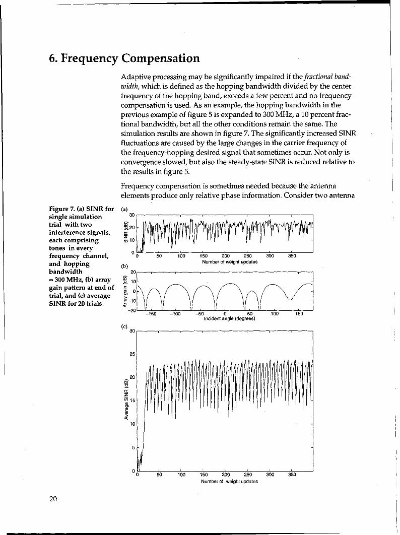
7. (a) SINR for single simulation trial with two interference signals, each comprising tones in every frequency channel, and hopping bandwidth = 300 MHz, (b) array gain pattern at end of trial, and (c) average SINR for 20 trials . . . . . . . . . . . . . . . . . . . . . . . . . . . . . . . . . . . . . . . . . . . . . . . . . . . . . . . . . . . . . . . . . . . . . . . . . 20

8. Two antenna elements of adaptive array receiving plane wave . . . . . . . . . . . . . . . . . . . . . . . . . . . . . . . . . . . . . . . . . . . . . . . . . . . 21 9. Basic configuration of adaptive array with anticipative processing . . . . . . . . . . . . . . . . . . . . . . . . . . . . . . . . . . . . . . . . . . . . 23

Tables

1. System parameters .............................................................................................................................. 14 2. Simulation results with edge length = a.. ......................................................................................... 18 3. Simulation results with edge length = 2it.. ....................................................................................... 19 4. Simulation results with edge length = . and total hopping bandwidth = 300 MHz.. .............. .25

1. Introduction

The maximin algorithm is an adaptive-array algorithm that suppresses interference before it enters the demodulator of a frequency-hopping communication system and thereby provides a spatial processing gain that supplements the inherent processing gain of the frequency-hopping system [l-3]. The algorithm discriminates between the desired signal and the interference on the basis of the distinct spectral characteristics of frequency-hopping signals. The maximin algorithm is so named because the desired signal is enhanced and the interference is suppressed simultaneously The maximin algorithm is a blind adaptive algorithm. Blind algorithms do not require training sequences, decision-directed adaptation, or knowledge of the direction of the desired signal, but instead rely on the basic characteristics of the desired-signal waveform. The maximin algorithm requires only that the frequency-hopping pattern must be known by the receiver.

1

I

2. Derivation

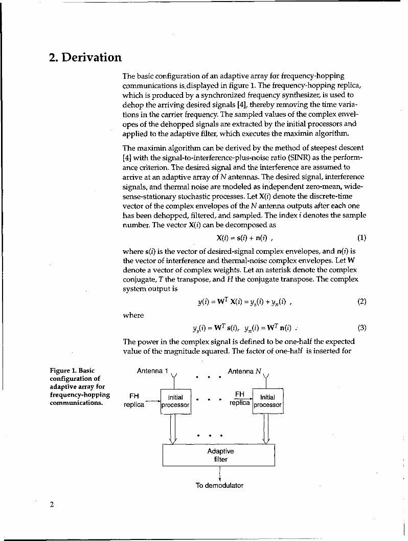
The basic configuration of an adaptive array for frequency-hopping communications is. displayed in figure 1. The frequency-hopping replica, which is produced by a synchronized frequency synthesizer, is used to dehop the arriving desired signals [4], thereby removing the time variations in the carrier frequency. The sampled values of the complex envelopes of the dehopped signals are extracted by the initial processors and applied to the adaptive filter, which executes the maximin algorithm.

The maximin algorithm can be derived by the method of steepest descent [4] with the signal-to-interference-plus-noise ratio (SINR) as the performance criterion. The desired signal and the interference are assumed to arrive at an adaptive array of N antennas. The desired signal, interference signals, and thermal noise are modeled as independent zero-mean, wide- sense-stationary stochastic processes. Let X(i) denote the discrete-time vector of the complex envelopes of the N antenna outputs after each one has been dehopped, filtered, and sampled. The index i denotes the sample number. The vector X(i) can be decomposed as

X(i) = s(i) + n(i) , (1) where s(i) is the vector of desired-signal complex envelopes, and n(i) is the vector of interference and thermal-noise complex envelopes. Let W

denote a vector of complex weights. Let an asterisk denote the complex conjugate, T the transpose, and H the conjugate transpose. The complex system output is

y(i) = WT X(i) = y,_(i) + y,(i) , (2) where

y,(i) = WT s(i), y,(i) = W* n(i) .’ (3)

The power in the complex signal is defined to be one-half the expected value of the magnitude squared. The factor of one-half is inserted for

Figure 1. Basic configuration of adaptive array for frequency-hopping communications.

Antenna 1 . . .

FH Initial . . . FH replica processor

. . . V V

Adaptive filter

I

+ To demodulator

2

consistency with the convention that the power in the complex envelope s(i) is equal to the power in the original bandpass signal (e.g., see Proakis [5]). If W is regarded as deterministic, the desired-signal output power is

‘s = # E[ 1 Y$) 1’1 = $ WHR,,W , (4)

where R,, is the desired-signal correlation matrix,

Rss = E[s*(i) sT(i)] , (5)

and E[x] denotes the expected value of x. The interference-plus-noise output power is

P =LWHR n 2

W nn ’ (6)

where R,, is the interference-plus-noise correlation matrix

R,, = E[n*(i) nT(i)] .

The SINR is

(7)

+ WHR,,W

n WHRn,W * (8)

To use the method of steepest descent in deriving an adaptive algorithm, it is necessary to calculate the gradient of the SINR with respect to the weight vector. In terms of its real part WR and its imaginary part WI, a complex weight vector is defined as

W=W,-jW,, (9)

where j = a. Let V~R and Vwr denote the gradients with respect to W, and WI, respectively. The complex gradient with respect to W is defined as

v,=v WR-I’%1 - (10)

A direct calculation using equations (4) and (6) gives

Let T, denote the time interval between samples. Let m denote the number of samples between weight iterations. The time interval between weight iterations is m T,. The method of steepest descent for discrete-time systems gives the recursive equation for the weight vector:

W(k + 1) = W(k) + p&k) v(k) (12)

where k denotes the weight iteration number, M(k) is a scalar sequence that controls the rate of change in the weight vector, ande(k) is an estimate of the gradient in equation (11) at iteration k. The ideal steepest- descent algorithm results if IV(k) is set equal to equation (11) with W(k) in place of W. However, this algorithm requires the estimation of Rllll, which is unknown in general, and Rss, which is unknown in the absence of information about the direction of the desired signal. To avoid the direct

3

estimation of these two matrices, several approaches are possible. If the desired signal is assumed to be narrowband, then an approximate linear- ization [4] of equation (11) leads to the Howells-Applebaum algorithm. Other approximations lead to the Shor feedback loop [6], which does not completely specify an adaptive algorithm. A third approach leads to the maximin algorithm, which is developed here.

The discrete-time vector s(i) is obtained from a continuous-time vector S(f) of complex envelopes. Each component of S(f) can be decomposed as

SJt) = SiR(t) + j Sir(t), i = 1,2, . . . , N , (13)

where SiR(f) is the real part or in-phase component of Si(f), and SiI(f) is the imaginary part or quadrature component of Si(f). Each S&f), i = 1,2, . . . , N, is a delayed version of the first component &l(f), which is modeled as a zero-mean, wide-sense stationary process. Two fundamental properties of the components of a complex envelope are [4,5]

E[ S lRW s lRcf + @] = E[ S lItf> s lrtf + @]

E[S,,(t) S,,(f + r)] = - EISlr(f) S,,(f + T)] ,

(14)

(15)

where r is an arbitrary delay Using these equations, we obtain

E[s(i) ST(i)] = 0 . (16)

The desired-signal component of the adaptive-filter output can be decomposed as

!&) = Y&) + j Y&) I (17)

where y&i) and ys.i) are the real and imaginary parts of y,(i), respectively. If the weight vector is treated as a constant W, then equations (3), (16), and (17) imply that

E[s*(i) ysR(i)] = E

/

s*(i) (t sT(i)W + + sH(i)W*} = $ E[s*(i) ST(i)] W . (18)

This equation and equation (5) yield

R,, w = 2 E[s*(i) y&i)] . (19)

Similarly, if the interference arriving at each antenna is a delayed version of the interference arriving at antenna 1, and if the thermal noise is independent in each array branch, then

E[n(i) nT(i)] = 0 , (20)

and, hence,

R,, W = 2 W+(i) y&i)] , (21)

4

I

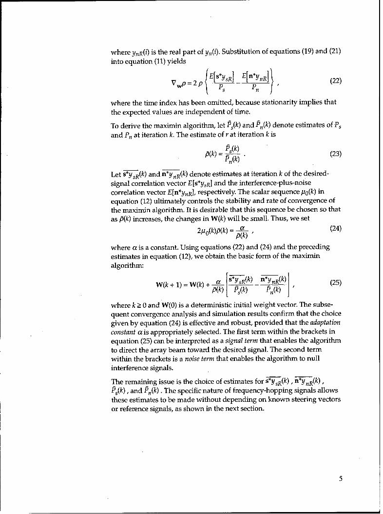
where ynR(i) is the real part of yn(i). Substitution of equations (19) and (21) into equation (11) yields

V,P=2P E[ %R] E[ n*%zR]

p - p I

S n (22)

where the time index has been omitted, because stationarity implies that the expected values are independent of time.

To derive the maximin algorithm, let ps(k) and pn(k) denote estimates of I’, and Pn at iteration k. The estimate of rat iteration k is

(23)

Let s*y,~(k) and n*ynR(k) denote estimates at iteration k of the desired- signal correlation vector E[s*Y,R] and the interference-plus-noise correlation vector E[n*y,R], respectively. The scalar sequence PO(k) in equation (12) ultimately controls the stability and rate of convergence of the maximin algorithm. It is desirable that this sequence be chosen so that as B(k) increases, the changes in W(k) will be small. Thus, we set

where a is a constant. Using equations (22) and (24) and the preceding estimates in equation (12), we obtain the basic form of the maximin algorithm:

(24)

W(k + 1) = W(k) + -E

I

s*y,R(k) n*!/,Rtk)

P(k) p&k) - p,(k) ’ I (25)

where k 2 0 and W(0) is a deterministic initial weight vector. The subsequent convergence analysis and simulation results confirm that the choice given by equation (24) is effective and robust, provided that the adaptation constant a is appropriately selected. The first term within the brackets in equation (25) can be interpreted as a signal term that enables the algorithm to direct the array beam toward the desired signal. The second term within the brackets is a noise term that enables the algorithm to null interference signals.

The remaining issue is the choice of estimates for s*y,#) , n*y,@ , P&k), and PJk) . The specific nature of frequency-hopping signals allows these estimates to be made without depending on known steering vectors or reference signals, as shown in the next section.

5

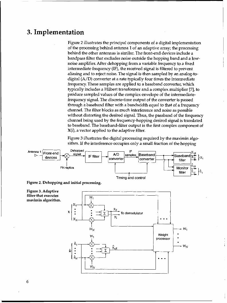
3. Implementation

Figure 2 illustrates the principal components of a digital implementation of the processing behind antenna 1 of an adaptive array; the processing behind the other antennas is similar. The front-end devices include a bandpass filter that excludes noise outside the hopping band and a low- noise amplifier. After dehopping from a variable frequency to a fixed intermediate frequency (IF), the received signal is filtered to prevent aliasing and to reject noise. The signal is then sampled by an analog-to- digital (A/D) converter at a rate typically four times the intermediate frequency. These samples are applied to a baseband converter, which typically includes a Hilbert transformer and a complex multiplier [7], to produce sampled values of the complex envelope of the intermediate- frequency signal. The discrete-time output of the converter is passed through a baseband filter with a bandwidth equal to that of a frequency channel. The filter blocks as much interference and noise as possible without distorting the desired signal. Thus, the passband of the frequency channel being used by the frequency-hopping desired signal is translated to baseband. The baseband-filter output is the first complex component of X(i), a vector applied to the adaptive filter.

Figure 3 illustrates the digital processing required by the maximin algorithm. If the interference occupies only a small fraction of the hopping

Antenna ’ Front-end D- devices

Dehopped IF signal A/D samples Baseband

-‘lR

* IF filter ----c. converter

i---C-Baseband G converter -

x, . filter -+ 1

FH replica

1 Timing and control

I:lR . Monitor -

Figure 2. Dehopping and initial processing.

Figure 3. Adaptive filter that executes maximin algorithm.

To demodulator

6

band, then it is usually absent from X(i) and yx(i). As the weights converge to their steady-state values, the interference component of YR(I’) becomes small, even if the interference is present in X(i). Thus, if the noise power is much less than the desired-signal power, then a suitable estimate of the desired-signal correlation vector is

where yR(i) is the real part of the adaptive-filter output y(i) given in equation (2).

An analogous estimate for n*y,&) is not possible, because when the system hops into a part of the band with interference power, then both the desired signal and the interference are imbedded in X(i). Instead, the receiver observes the interference and noise in a nearby frequency channel that is not currently being used by the desired signal, but will be after a subsequent frequency hop. After a frequency translation, the interference and noise in the nearby monitored channel are extracted by each antenna’s monitor filter from the baseband converter output, as shown in figure 2. The intermediate-frequency filter must have a passband large enough to encompass-both the downconverted frequency channel being used by the desired signal and the downconverted monitored channel.

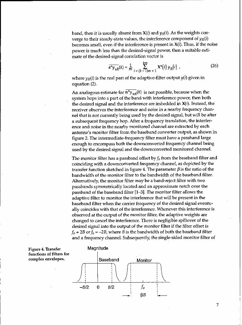
The monitor filter has a passband offset byfo from the baseband filter and coinciding with a downconverted frequency channel, as depicted by the transfer function sketched in figure 4. The parameter p is the ratio of the bandwidth of the monitor filter to the bandwidth of the baseband filter. Alternatively, the monitor filter may be a band-reject filter with two passbands symmetrically located and an approximate notch over the passband of the baseband filter [l-3]. The monitor filter allows the adaptive filter to monitor the interference that will be present in the baseband filter when the carrier frequency of the desired signal eventu- ally coincides with that of the interference. Whenever this interference is observed at the output of the monitor filter, the adaptive weights are changed to cancel the interference. There is negligible spillover of the desired signal into the output of the monitor filter if the filter offset is fO = 2B orfo = -2B, w h ere B is the bandwidth of both the baseband filter and a frequency channel. Subsequently, the single-sided monitor filter of

Figure 4. Transfer Magnitude functions of filters for complex envelopes. Baseband

I I I I I I I 1

i\)y-T\

I

-B/2 0 B/2 I I I I h ;

-I PB Ia-

figure 4 with /I = 1 is assumed, because then the monitor filter passes almost exactly the same interference waveforms as are subsequently passed by the baseband filter.

When the carrier frequency is at or near one of the ends of the hopping band, the monitor filter will not be able to observe interference in the hopping band. However, this effect will be of negligible importance when there are a large number of carrier frequencies.

Let A(i) denote the vector of N discrete-time outputs of the monitor filters and define

9,(i) = wT(i) ii(i) .

The vector

ne(i) = ii(i) exp (-j2 nfo T,)

(27)

(28)

provides an estimate of the baseband-filter input n(i) that will occur when the desired-signal carrier frequency is such that the interference and noise currently in the monitor filter enter the baseband filter. Treating the weight vect r as a con tant so that equation (21) is valid and assuming thatR,,=Epn:(i)nF(id,weobtain

E[n*(i) ynR(i)] = i E[nl(i) n:(i)] W(i) . (2%

From equation (20), it is reasonable to assume that E[ n&i) n:(i)] = 0 . This assumption and equations (27) to (29) yield

E[n*(i) y,~i)] = E $ iiT W(i) + 5 AH(i) W*(i)

(30)

= E[ fi*(i) YOU’D] , where YnR(i) is the real part of P,(i) . This equation implies that a suitable estimate is

(31)

The estimate I?,(k) can be simplified by observing from a straightforward

calculation using equations (3), (16), and (17) that E[y$] = E[&] , so that

equation (4) implies that pS = ~[y,2R] = E[yi] . Similarly, 1”, = ~[y&] = +&a] . Th ere f ore, suitable power estimates are obtained by computing

(32)

(33)

8

In applications where the desired signal may sometimes be absent, it may

be necessary to lower-bound pS(k) by a small positive number chosen to prevent a possible singularity in the maximin algorithm.

The estimates in equations (26), (31), (32), and (33) complete the specifica- tion of the maximin algorithm given by equation (25). If the underlying assumptions are changed, then different versions of these estimates, and hence of the maximin algorithm, result. For example, if the interference occupies large spectral regions of the hopping band, then usually ye will contain significant interference power before the weights converge. To compensate for this power, closely related alternative versions of the maximin algorithm can be derived [l-3]. However, many simulation experiments indicate that the version of the algorithm derived above is the most flexible, nearly always gives a similar or better performance than alternative versions, and is computationally the simplest.

During acquisition of the frequency-hopping pattern, the frequency synthesizer produces different frequencies from those of the received frequency-hopping pulses. Consequently, the desired signal is usually absent from the outputs of the baseband filters, and the maximin algorithm must be modified. During acquisition, a suitable adaptive algorithm is the recursive suppression algorithm [8], which tends to suppress signals arriving from any direction. Cancellation of the desired signal is avoided because of its infrequent appearance in the outputs of the baseband and monitor filters.

During acquisition, the adaptive system forms nulls in the directions of the interference signals, thereby assisting the receiver in synchronizing with the received frequency-hopping signal. Although a grating null might be inadvertently placed on the desired signal during acquisition, the probability of this event can usually be kept small by appropriate placement of the antenna elements [6]. After acquisition is confirmed by the receiver, it activates the maximin algorithm.

9

4. Convergence Analysis

A frequency-hopping signal consisting of pulses transmitted at many different frequencies is a wideband signal. However, the frequency channel associated with a single pulse is usually narrow. Thus, although a frequency-hopping signal may hop over a wide band, it has a narrow instantaneous bandwidth. For a narrowband desired signal, the vector of sampled complex envelopes is well approximated by [4,6]

s(i) = s&i) s, , (34)

where sl(i) is the sampled complex envelope at antenna 1, which serves as a reference point, and So is a steering vector. If the antenna patterns are identical and the antennas are close enough that the signal amplitudes at all the antennas are nearly the same, then component i of the steering vector is exp(ij 2 nfc Ti), where fc is the center frequency and Ti, 2 I i I N,

is the arrival-time delay at antenna i relative to antenna 1. After the substitution of equations (5) and (34) into equation (8), the maximization of the SINR yields the optimal weight vector [4,6]

W, = qR,,1 S;, , (35)

where 77 is an arbitrary constant, and the superscript -1 denotes the inverse. For those pulses that hop over a sufficiently small.band within the hopping band, the optimal weight vector is well approximated by equation (35), with SO evaluated at the center frequency of the small band.

The highly nonlinear nature of the maxirnin algorithm precludes a completely rigorous convergence analysis. However, with enough approximations, the convergence of the mean weight vector to Wo can be demon- strated and bounds on the adaptation constant can be derived. Assume that enough algorithm iterations have occurred that the power estimates are well approximated by the values they would have if the weight vector were equal to Wo. The desired-signal power at an antenna is

P,i=~E[/S,(i)12] I (36)

Using equations (4), (5), (34), (35), and (36), and the fact that Rlzn is Hermi- tian, we obtain

Similarly,

Id2 f,(k) = P,, = $ W,H R,, W. = 2 S; R,1, S; .

Equations (37) and (38) imply that

(37)

10

Assuming the zero-mean stationarity of the signals and the independence of the desired-signal and the interference-plus-noise, we obtain from equations (26), (l), and (2) that

E[ K&k)] = E[ X”( i) Yx( i,]

= E[ s”(i) Y,x(‘)] + E[ n*(i) Y,,(i)] (40)

*

Equation (25) indicates that W(k + 1) depends on S(Z) and n(l) for I5 k, but not directly on S(k + 1) and n(k + 1). Therefore, we make the approxima- tion that W(k) is statistically independent of S(k) and n(k). A calculation similar to equation (18) using equations (16) and (20) then yields

E[ sly,R(k)] = $( R, + R,,) E[W(k)] - (41)

Similarly, equations (30) and (31) imply that

E[n*Y,X(k)] = $ R,, E[W(k)] . WI

Taking the expected value of both sides of equation (25), substituting equations (37) to (42), and simplifying algebraically, we obtain

(p. - 1) R,, -R,, E[VO] t (43)

where k L 0 and E[W(O)] = W(0). Assuming that p. P 1, we set p. - 1= p.

and define

D = PO R,, - R,, . kw

We obtain the approximate result

(45)

A straightforward calculation using equations (5), (34), (36), and (39) yields

DR,1,S;=O. (46)

This equation indicates that R$ Si * IS an eigenvector of D, and the corresponding eigenvalue is 0. Since D is HermitianGit has a complete set of N orthogonal eigenvectors, one of which is R$ So . Thus, we can make the decomposition

E[ W(k)] = q(k) R;i S i + yg: a $4 e i , (47)

where each ai and q(k) are scalar functions and ei is one of the N - 1 eigenvectors orthogonal to R ,A Si . Substituting equation (47) into equation (45) and using the orthogonality of the eigenvectors, we obtain

q(k + I) = q(k) = 77 (48)

aJk+ 1) = l- ai( i = 1,2,. . . , N - 1 , (49)

11

where 77 is an arbitrary constant and 4 is the eigenvalue corresponding to ei. Equations (48), (47), and (35) give

E[ W(k)] = Wo + ygll a i(k) e i ,

which implies that E[W(k)] converges to Wo if and only if each ai converges to 0. From equation (49), it follows that

ai = l-

Therefore, az(k) converges to 0 if and only if

l- 2 Pypso iii <l , i=l,2 ,..., N-l .

(50)

(51)

(52)

As shown subsequently, each 4 is positive. Equation (52) yields the necessary and sufficient convergence condition for the convergence of

E[W(k)]:

4 PO pso O<a< il , (53) max

where Lax is the largest eigenvalue of D.

It remains to show that each 4 is positive. Since the SINR is maximized when W = Wo, it follows from equation (8) that

WH R,, W

WH R,, W <PO f (54)

where the inequality is strict when W f WO. Combining equations (44) and (54) gives

WHDW20, (55)

which proves that the Hermitian matrix D is nonnegative definite. Hence all its eigenvalues must be nonnegative. Since only W = Wo gives an equality in equation (55), setting W = ei implies that

erDei>O, i=l,2 ,..., N-l . (56)

Therefore, 4 = 0 is impossible and

;li>O, i=l,2 ,..., N-l . (57)

The sum of the eigenvalues of a square martrix is equal to its trace. Thus,

amax 5 yg: ai = tr(D) = p$r(R,,) - tr(R,,)

(58)

5 p,tr( R,,) I

where tr(A) denotes the trace of A. Consequently, equation (53) implies that

(59)

12

is a sufficient condition (but not a necessary condition) for the convergence of the mean weight vector to the optimal weight vector.

Assume the interference-plus-noise power in each component of n(i) is

equal to Pni. Then tr(R& = 2N P,i. Let 1 z 1 denote the Euclidean norm of a

vector z. From equations (5), (34), (36), and (37) and the Schwarz inequal-

ity, it follows that Pss, 5 1 W, I2 1 So 1’ Psi . If each component of So is a

complex exponential, 1 So I2 = N and J’s’,0 5 N 1 Wo I2 Psi . Substituting

E[W(O)] = W(0) into equation (50) and using the orthogonal@ of the

eigenvectors gives 1 Wo I<: I W(O) I . Therefore, the upper bound a, = 4 P,,/

tr R,, in equation (59) is approximately bounded by

where p1 = P,JP,i is the SINR in a single baseband-filter output prior to the adaptive filtering and equals the SINR per frequency channel at an antenna input. Since the bound in this inequality is easily calculated, it provides a useful, albeit imperfect, guide in selecting the appropriate value of the adaptation constant.

13

5. Description of Simulation

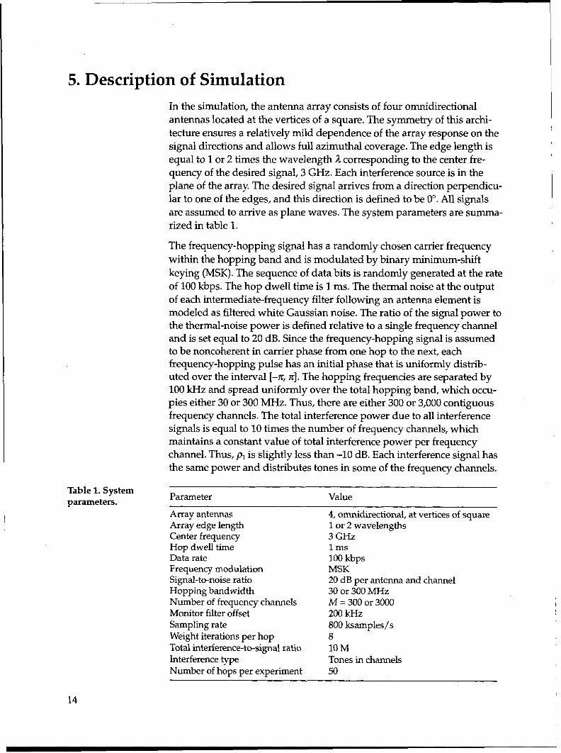
In the simulation, the antenna array consists of four omnidirectional antennas located at the vertices of a square. The symmetry of this archi- tecture ensures a relatively mild dependence of the array response on the signal directions and allows full azimuthal coverage. The edge length is equal to 1 or 2 times the wavelength ;1 corresponding to the center frequency of the desired signal, 3 GHz. Each interference source is in the plane of the array The desired signal arrives from a direction perpendicular to one of the edges, and this direction is defined to be 0”. All signals are assumed to arrive as plane waves. The system parameters are summarized in table 1.

The frequency-hopping signal has a randomly chosen carrier frequency within the hopping band and is modulated by binary minimum-shift keying (MSK). The sequence of data bits is randomly generated at the rate of 100 kbps. The hop dwell time is 1111s. The thermal noise at the output of each intermediate-frequency filter following an antenna element is modeled as filtered white Gaussian noise. The ratio of the signal power to the thermal-noise power is defined relative to a single frequency channel and is set equal to 20 dB. Since the frequency-hopping signal is assumed to be noncoherent in carrier phase from one hop to the next, each frequency-hopping pulse has an initial phase that is uniformly distrib- uted over the interval [-n, ~1. The hopping frequencies are separated by 100 kHz and spread uniformly over the total hopping band, which occupies either 30 or 300 MHz. Thus, there are either 300 or 3,000 contiguous frequency channels. The total interference power due to all interference signals is equal to 10 times the number of frequency channels, which maintains a constant value of total interference power per frequency channel. Thus, p1 is slightly less than -10 dB. Each interference signal has the same power and distributes tones in some of the frequency channels.

Table 1. System parameters.

Parameter Value

Array antennas Array edge length Center frequency Hop dwell time Data rate Frequency modulation Signal-to-noise ratio Hopping bandwidth Number of frequency channels Monitor filter offset Sampling rate Weight iterations per hop Total interference-to-signal ratio Interference type Number of hops per experiment

4, omnidirectional, at vertices of square 1 or 2 wavelengths 3 GHz lms 100 kbps MSK 20 dB per antenna and channel 30 or 300 MHz M = 300 or 3000 200 kHz 800 ksamples/s 8 10M Tones in channels 50

14

Perfect synchronization between the frequency-hopping signals at all the antenna outputs and the frequency synthesizer in the receiver is assumed. The baseband and monitor filters are modeled as digital S-pole Butter- worth filters with the 3-dB bandwidths equal to 100 kHz, the bandwidth of a frequency channel. The monitor filter has a single passband, as depicted in figure 4, with parametersf, = 200 kHz and /? = 1. The sampling rate of the analog-to-digital converter is 800 kilosamples per second. There are 8 weight iterations per hop.

In each of the subsequent simulation experiments, the initial weight vector is W(0) = Wbeam, where

W beam = f1 1 1 1 1 . (61)

This weight vector points the array beam or gain pattern in the direction of the desired signal. Thus, the subsequent simulation experiments indicate the performance of the maximin algorithm after the sudden appearance of interference from various directions. An alternative is to set W(0) = Womni, where

W omni=[ 1 0 0 01.

This weight vector corresponds to an omnidirectional gain pattern. Its use as the initial weight vector is appropriate if one wishes to assess the convergence of the maximin algorithm from a cold start. Since the algorithm then has to form a beam in the direction of the desired signal while simultaneously attempting to null the interference signals, the convergence is slowed relative to what it would be if W(0) = Wbeam. Simulation experiments verify that the steady-state performance is not affected by the choice of Wbeam or Womni as the initial weight vector, so Abeam is always used.

Inequalities (59) and (60) indicate that 0 < a SQ, where a, I 0.8 is sufficient for convergence if the interference signals approximate stationary processes. Simulation experiments confirm that the maximin algorithm does converge to a steady state when 0 < GI I 0.8. It is found that a = 0.2 usually provides close to the fastest convergence and the best performance when each interference signal comprises tones in every frequency channel.

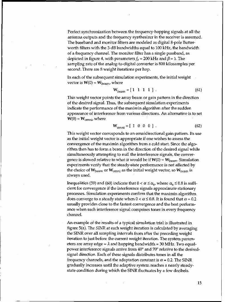
An example of the results of a typical simulation trial is illustrated in figure 5(a). The SINR at each weight iteration is calculated by averaging the SJNR over all sampling intervals from after the preceding weight iteration to just before the current weight iteration. The system parameters are array edge = il and hopping bandwidth = 30 MHz. Two equal- power interference signals arrive from 40” and 70” relative to the desired- signal direction. Each of these signals distributes tones in all the frequency channels, and the adaptation constant is a = 0.2. The SINR gradually increases until the adaptive system reaches a nearly steady- state condition during which the SINR fluctuates by a few decibels.

15

Figure 5. (a) SINR for single simulation trial with two interference signals, each comprising tones in every frequency channel, and hopping bandwidth = 30 MHz, (b) array gain pattern at end of trial, and (cl average SINR for 20 trials.

-0 50 100 150 200 250 300 350

(b) Number of weight updates

is E IO-

-_ -150 -100 -50 0 50 100 150

Incident angle (degrees)

(cl 30 1 I I I

25

II

0 50 100 150 200 250 300 350 Number of weight updates

Figure 5(b) depicts the array gain pattern at the end of the simulation trial. There are nulls of less than -20 dB in the directions of the interference sources. Figure 5(c) shows the average SINR, which is defined as the SINR obtained by averaging over 20 simulation trials at each weight iteration.

If each interference signal independently distributes tones of equal power in every fourth frequency channel to cover 25 percent of the hopping band, then the simulation results are quite different. As shown in figures 6(a) and (c), the convergence is slowed and the fluctuations in SlNR are increased, because the monitor filter only observes each interference signal 25 percent of the time. Between these observations, the weights tend to slowly drift toward the values they would have without the interference. This drift and the occasional large interference levels force the lowering of the adaptation constant to obtain good algorithm convergence, and a = 0.05 is used to generate figure 6. Figure 6(b)

16

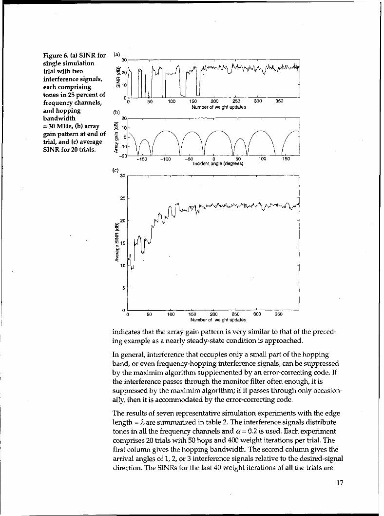
Figure 6. (a) SINR for single simulation trial with two interference signals, each comprising tones in 25 percent of frequency channels, and hopping bandwidth = 30 MHz, (b) array gain pattern at end of trial, and (cl average SINR for 20 trials.

0 I, 0 50 100 150 200 250 300 350

Number of weight updates 04

20, , I I I

Incident angle (degrees)

@) 30 ,

25 -

0’ 0 50 100 150 200 250 300 350

Number of weight updates

indicates that the array gain pattern is very similar to that of the preceding example as a nearly steady-state condition is approached.

In general, interference that occupies only a small part of the hopping band, or even frequency-hopping interference signals, can be suppressed by the maximim algorithm supplemented by an error-correcting code. If the interference passes through the monitor filter often enough, it is suppressed by the maximim algorithm; if it passes through only occasion- ally, then it is accommodated by the error-correcting code.

The results of seven representative simulation experiments with the edge length = ;3. are summarized in table 2. The interference signals distribute tones in all the frequency channels and a! = 0.2 is used. Each experiment comprises 20 trials with 50 hops and 400 weight iterations per trial. The first column gives the hopping bandwidth. The second column gives the arrival angles of 1,2, or 3 interference signals relative to the desired-signal direction. The SINRs for the last 40 weight iterations of all the trials are

17

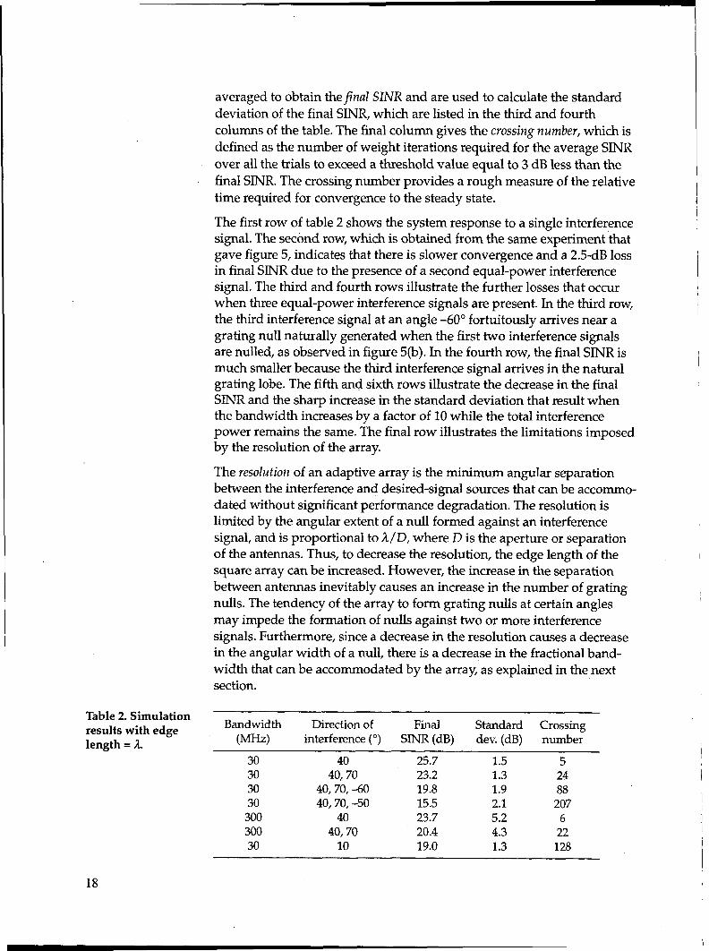
averaged to obtain thefinal SINR and are used to calculate the standard deviation of the final SINR, which are listed in the third and fourth columns of the table. The final column gives the crossing number, which is defined as the number of weight iterations required for the average SINR over all the trials to exceed a threshold value equal to 3 dB less than the final SlNR. The crossing number provides a rough measure of the relative time required for convergence to the steady state.

The first row of table 2 shows the system response to a single interference signal. The second row, which is obtained from the same experiment that gave figure 5, indicates that there is slower convergence and a 2.5-dB loss in final SINR due to the presence of a second equal-power interference signal. The third and fourth rows illustrate the further losses that occur when three equal-power interference signals are present. In the third row, the third interference signal at an angle -60” fortuitously arrives near a grating null naturally generated when the first two interference signals are nulled, as observed in figure 5(b). In the fourth row, the final SINR is much smaller because the third interference signal arrives in the natural grating lobe. The fifth and sixth rows illustrate the decrease in the final SINR and the sharp increase in the standard deviation that result when the bandwidth increases by a factor of 10 while the total interference power remains the same. The final row illustrates the limitations imposed by the resolution of the array.

The reso2ution of an adaptive array is the minimum angular separation between the interference and desired-signal sources that can be accommodated without significant performance degradation. The resolution is limited by the angular extent of a null formed against an interference signal, and is proportional to L/D, where D is the aperture or separation of the antennas. Thus, to decrease the resolution, the edge length of the square array can be increased. However, the increase in the separation between antennas inevitably causes an increase in the number of grating nulls. The tendency of the array to form grating nulls at certain angles may impede the formation of nulls against two or more interference signals. Furthermore, since a decrease in the resolution causes a decrease in the angular width of a null, there is a decrease in the fractional bandwidth that can be accommodated by the array, as explained in the next section.

Table 2. Simulation results with edge length = ;t.

Bandwidth Direction of Final Standard Crossing (MHz) interference (“) SINR (dB) dev. (dB) number

30 40 25.7 1.5 5 30 40,70 23.2 1.3 24 30 40,70, -60 19.8 1.9 88 30 40,70, -50 15.5 2.1 207

300 40 23.7 5.2 6 300 40,70 20.4 4.3 22 30 10 19.0 1.3 128

18

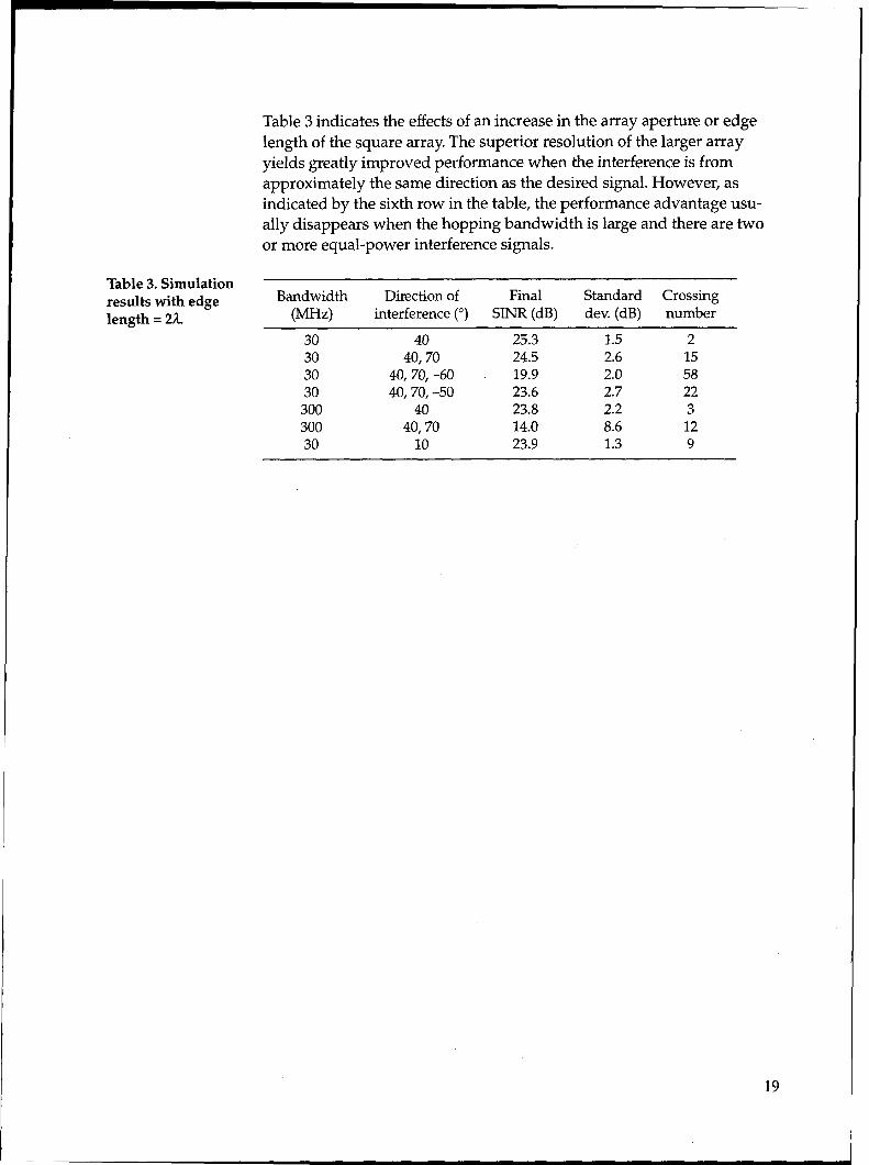
Table 3 indicates the effects of an increase in the array aperture or edge length of the square array. The superior resolution of the larger array yields greatly improved performance when the interference is from approximately the same direction as the desired signal. However, as indicated by the sixth row in the table, the performance advantage usually disappears when the hopping bandwidth is large and there are two or more equal-power interference signals.

Table 3. Simulation results with edge length = 2h

Bandwidth Direction of Final Standard Crossing

W-W interference (“) SINR (dB) dev. (dB) number

30 40 25.3 1.5 2 30 40,70 24.5 2.6 15 30 40, 70, -60 19.9 2.0 58 30 40,70, -50 23.6 2.7 22

300 40 23.8 2.2 3 300 40,70 14.0 8.6 12 30 10 23.9 1.3 9

6. Frequency Compensation

Figure 7. (a) SINR for single simulation trial with two interference signals, each comprising tones in every frequency channel, and hopping bandwidth = 300 MHz, (b) array gain pattern at end of trial, and (cl average SINR for 20 trials.

Adaptive processing may be significantly impaired if thefvactional bandwidth, which is defined as the hopping bandwidth divided by the center frequency of the hopping band, exceeds a few percent and no frequency compensation is used. As an example, the hopping bandwidth in the previous example of figure 5 is expanded to 300 MHz, a 10 percent fractional bandwidth, but all the other conditions remain the same. The simulation results are shown in figure 7. The significantly increased SINR fluctuations are caused by the large changes in the carrier frequency of the frequency-hopping desired signal that sometimes occur. Not only is convergence slowed, but also the steady-state SINR is reduced relative to the results in figure 5.

Frequency compensation is sometimes needed because the antenna elements produce only relative phase information. Consider two antenna

(4


20, I I I

~_~~~(y-y--)~,~-\i -20’ ” 1 ’

-150 -100 -50 0 50 100 150 Incident angle (degrees)

@) 30, 1 I I I

,I 0 50 100 150 200 250 300 350


20

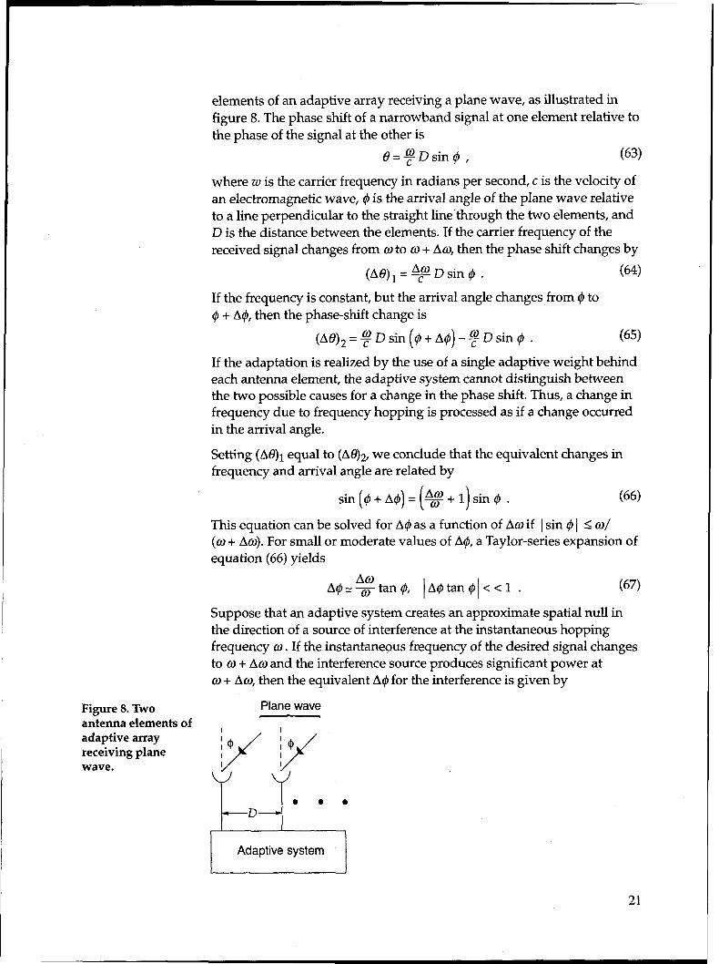
Figure 8. Two antenna elements of adaptive array receiving plane wave.

elements of an adaptive array receiving a plane wave, as illustrated in figure 8. The phase shift of a narrowband signal at one element relative to the phase of the signal at the other is

8=+Dsin@, (63)

where w is the carrier frequency in radians per second, c is the velocity of an electromagnetic wave, 4 is the arrival angle of the plane wave relative to a line perpendicular to the straight line’through the two elements, and D is the distance between the elements. If the carrier frequency of the received signal changes from o to o + do, then the phase shift changes by

(A@), = F D sin 4 . (64)

If the frequency is constant, but the arrival angle changes from C#J to @ + A$, then the phase-shift change is

(A@, = $ D sin ($ + A@) - F 0 sin @ . (65)

If the adaptation is realized by the use of a single adaptive weight behind each antenna element, the adaptive system cannot distinguish between the two possible causes for a change in the phase shift. Thus, a change in frequency due to frequency hopping is processed as if a change occurred in the arrival angle.

Setting (AO), equal to (A@, we conclude that the equivalent changes in frequency and arrival angle are related by

sin(@+A@)=(@+l)sin@. (66)

This equation can be solved for A@ as a function of Ao if 1 sin @ 1 5 co/

(a + Aw). For small or moderate values of A$, a Taylor-series expansion of equation (66) yields

(67)

Suppose that an adaptive system creates an approximate spatial null in the direction of a source of interference at the instantaneous hopping frequency u . If the instantaneous frequency of the desired signal changes to o + Aw and the interference source produces significant power at w + AU, then the equivalent A@ for the interference is given by

Plane wave

Adaptive system

21

equations (66) and (67). If A.o is sufficiently large, A# may be larger than the angular width of the original null. Consequently, after the carrier frequency of the desired signal hops to w + A@, the interference is not immediately nulled, but further adaptation is required to again establish a spatial null. Thus, if the fractional bandwidth is large, then unless (1) the angular width of a null is large, (2) Ao is restricted to small values, or (3) some type of frequency compensation is adopted, the benefit of the adaptive processing may diminish significantly.

The angular width of a null can be increased by decreasing the separation among antennas in the array, but then the resolution may be increased to an unsatisfactory level. The restriction of the frequency change after a hop Aw to a small value keeps the interference near the center of a spatial null and makes it possible for the adaptive system to rapidly increase the interference rejection. However, the variety of hopping patterns is reduced, which diminishes the resistance to frequency-selective fading and increases the susceptibility to wideband interference or jamming, Thus, frequency compensation is the preferred alternative.

Three basic methods of frequency compensation for frequency hopping are parameter-dependent, spectral, and anticipative processing. Parameter-dependent processing introduces additional parameters in an attempt to increase the angular extent and spectral bandwidth of the nulls. For the maximin algorithm, a compatible realization applies v successive discrete-time outputs of each baseband filter and each monitor filter as inputs to the adaptive filter, thereby increasing the number of weights in figure 3 by a factor of v. However, the filters sharply limit the degree of spectral or beam shaping that might be possible using the successive outputs. Simulation results confirm that parameter-dependent processing is ineffective for the maximin algorithm.

Specfrd processing is based on dividing the hopping band into a number of spectral regions and adapting independently when the carrier frequency is in one of the regions. The weights associated with each spectral region are stored in a memory within the weight processor of figure 3. At the end of the signal dwell time at a specific frequency, the weights of the adaptive filter are transferred to the memory. Then the weights associated with the new carrier frequency are transferred from the memory to the filter. These weights are updated during the time interval at the new frequency Transfers between the memory and the filter are controlled by the frequency-hopping code generator. The number of spectral regions N, is ultimately limited by the proportional increase in the required number of iterations to converge to steady state, because only l/N, of the frequency-hopping pulses are associated with each region. However, this increase is slowed by the contraction of each region as N, increases, which expedites the convergence within each region. The relatively slow convergence rate of spectral processing is its major disadvantage; its major advantage is its relatively simple implementation.

22

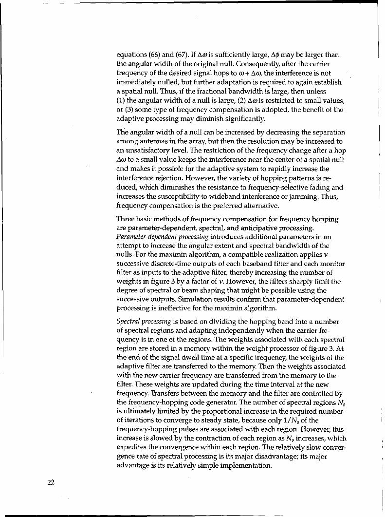
The desired signal is not present in the auxiliary processors because they monitor the frequency channel of the next hop. Consequently, baseband filters can be used as monitor filters to extract various estimates of the interference-plus-noise. These baseband filters allow narrower intermediate-frequency filters and, hence, a lower sampling rate in the auxiliary processor than in the main processor.

Figure 9. Basic configuration of adaptive array with anticipative

. processing.

An anticipative adaptive system begins adaptation toward the optimal weights for a carrier frequency before that frequency is transmitted. Anticipative processing with an auxiliary processor operating in parallel with the main processor is illustrated by figure 9. A time-advanced frequency-hopping replica hops one hopping period ahead of the replica used for dehopping the desired signal. While the main adaptive filter produces the output, the auxiliary filter adapts the weights corresponding to the next hopping frequency. After each hop, the weights associated with the new hopping frequency are transferred from the auxiliary filter to the main filter. Transfers are triggered by the clock that controls the frequency-hopping carrier transitions. The weight vector in the auxiliary filter is not necessarily updated at the same times as the weight vector in the main filter. The auxiliary filter may update its weight vector during the switching times between hops, but in the simulation, the duration of the switching time is assumed to be negligible.

Let W,(l) denote the anticipative weight vector computed by the auxiliary adaptive filter at iteration 2. The recursive equation for W,(l + 1) is derived by modifying the maximin algorithm to allow for the absence of the desired signal in the auxiliary filter and for the measurements by the auxiliary filter. Thus, the signal term within the brackets in equation (25) is discarded, and the remaining equation is simplified. The anticipative maximin algorithm is

wa(z + 1) = w,(z) - al [ “*YnRP)],

V) ’ (68)

where al is the anticipative adaptation constant and the subscript u on the bracketed factor indicates that it is measured by the auxiliary adaptive

Antennas 0 . 0

I /

t To

demodulator

23

filter, which uses the output of a frequency channel that will not be observed by the main adaptive filter until the next hop. The desired- signal power estimate p&l) is the most recent estimate computed by the main adaptive filter and is assumed to be nearly independent of the frequency channel. The bracketed factor is defined by equation (31), with ii(i) interpreted as the discrete-time vector of complex envelopes at the input of the auxiliary adaptive filter and ij&i) as the real part of the filter output.

The weight vector in the main adaptive filter is updated by computing equation (25), except at sampling instants occurring during switching times. At these instants, the weight vector in the main adaptive filter is set equal to that of the auxiliary adaptive filter. The switching times occur when k = nko in the main filter and i = nkl in the auxiliary filter, where b is the number of iterations per hop in the main filter, kl is the number of iterations per hop in the auxiliary filter, and n = 1,2, . . . is the hop number. Thus, the maximin algorithm in the main filter becomes

I , k+ l+nko

(69) W(nko) = W,(nkl) , n = 0, 1, . . . .

The anticipative maximin algorithm, which is closely related to the recursive suppression algorithm [8] for direction finding, attempts to null all signals with power in the hopping band, but does not null the desired signal because it is never present in the baseband filters of the auxiliary adaptive filter. This absence ultimately is due to the system’s knowledge of the frequency-hopping pattern.

One might consider a version of the anticipative maximin algorithm in which the signal term in equation (25) is retained. The signal term cannot be computed by the auxiliary adaptive filter because it does not receive the desired signal. Therefore, the signal term computed by the main adaptive filter is used to enable beamforming by the auxiliary adaptive filter in the direction of the desired signal. However, the signal term does not include frequency compensation, and any beamforming tends to erode the nulls when interference is absent in the monitor filter outputs. Simulation results indicate that this algorithm version can accommodate larger adaptation constants and, hence, expedites the convergence when the interference signals occupy all the frequency channels, but its performance is inferior when interference signals occupy only a fraction of the hopping band. Thus, equation (68) is the preferred form of the anticipative maximin algorithm.

The results of nine simulation experiments are displayed in table 4, where the edge length is a, the hopping bandwidth is 300 MHz, and the fractional bandwidth is 10 percent. The first three rows in table 4 give results for no frequency compensation and a = 0.2 as a reference for comparison.

24

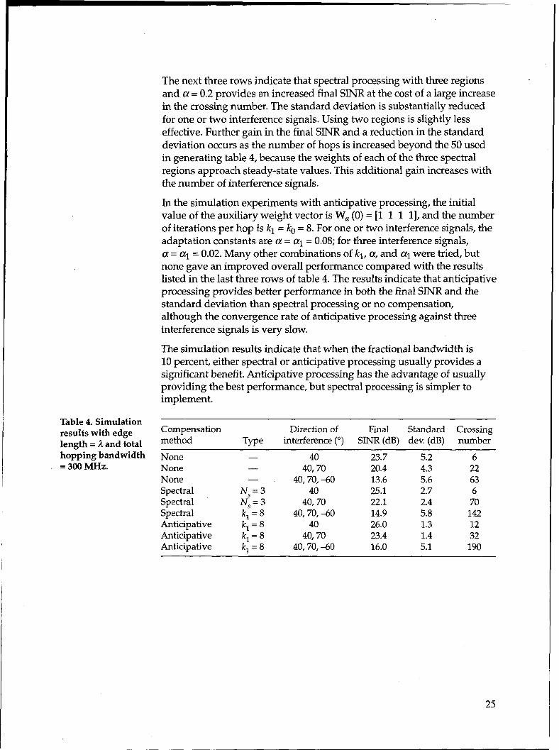
The next three rows indicate that spectral processing with three regions and a = 0.2 provides an increased final SINR at the cost of a large increase in the crossing number. The standard deviation is substantially reduced for one or two interference signals. Using two regions is slightly less effective. Further gain in the final SINR and a reduction in the standard deviation occurs as the number of hops is increased beyond the 50 used in generating table 4, because the weights of each of the three spectral regions approach steady-state values. This additional gain increases with the number of interference signals.

In the simulation experiments with anticipative processing, the initial value of the auxiliary weight vector is W, (0) = [l 1 1 11, and the number of iterations per hop is kl= b = 8. Fo r one or two interference signals, the adaptation constants are a = a1 = 0.08; for three interference signals, a = al = 0.02. Many other combinations of kl, a, and al were tried, but none gave an improved overall performance compared with the results listed in the last three rows of table 4. The results indicate that anticipative processing provides better performance in both the final SINR and the standard deviation than spectral processing or no compensation, although the convergence rate of anticipative processing against three interference signals is very slow.

The simulation results indicate that when the fractional bandwidth is 10 percent, either spectral or anticipative processing usually provides a significant benefit. Anticipative processing has the advantage of usually providing the best performance, but spectral processing is simpler to implement.

Table 4. Simulation results with edge Compensation Direction of Final Standard Crossing

length = A and total method Type interference (“) SINR (dB) dev. (dB) number

hopping bandwidth None - 40 23.7 5.2 6 = 300 MHz. None - 40,70 20.4 4.3 22

None - 40,70, -60 13.6 5.6 63 Spectral N,=3 40 25.1 2.7 6 Spectral N,=3 40,70 22.1 2.4 70 Spectral k, = 8 40,70, -60 14.9 5.8 142 Anticipative k, = 8 40 26.0 1.3 12 Anticipative k, = 8 40,70 23.4 1.4 32 Anticipative k, =8 40,70, -60 16.0 5.1 190

25

I

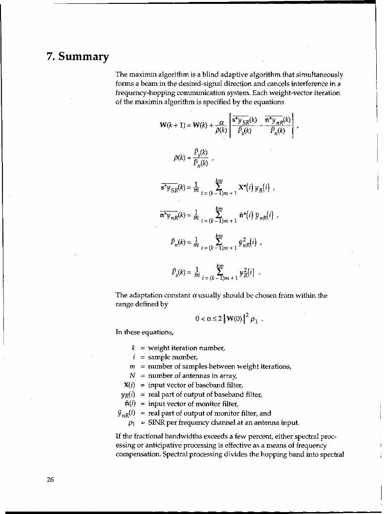
7. Summary

The maximin algorithm is a blind adaptive algorithm that simultaneously forms a beam in the desired-signal direction and cancels interference in a frequency-hopping communication system. Each weight-vector iteration of the maximin algorithm is specified by the equations

&(k) P(k) = f ,

II

km

The adaptation constant a usually should be chosen from within the range defined by

0<a12~W(0)12pl

In these equations,

N=

X(i) =

ydi) = ii(i) =

!Tn#) = Pl =

weight iteration number, sample number, number of samples between weight iterations, number of antennas in array, input vector of baseband filter, real part of output of baseband filter, input vector of monitor filter, real part of output of monitor filter, and SINR per frequency channel at an antenna input.

If the fractional bandwidths exceeds a few percent, either spectral processing or anticipative processing is effective as a means of frequency compensation. Spectral processing divides the hopping band into spectral

26

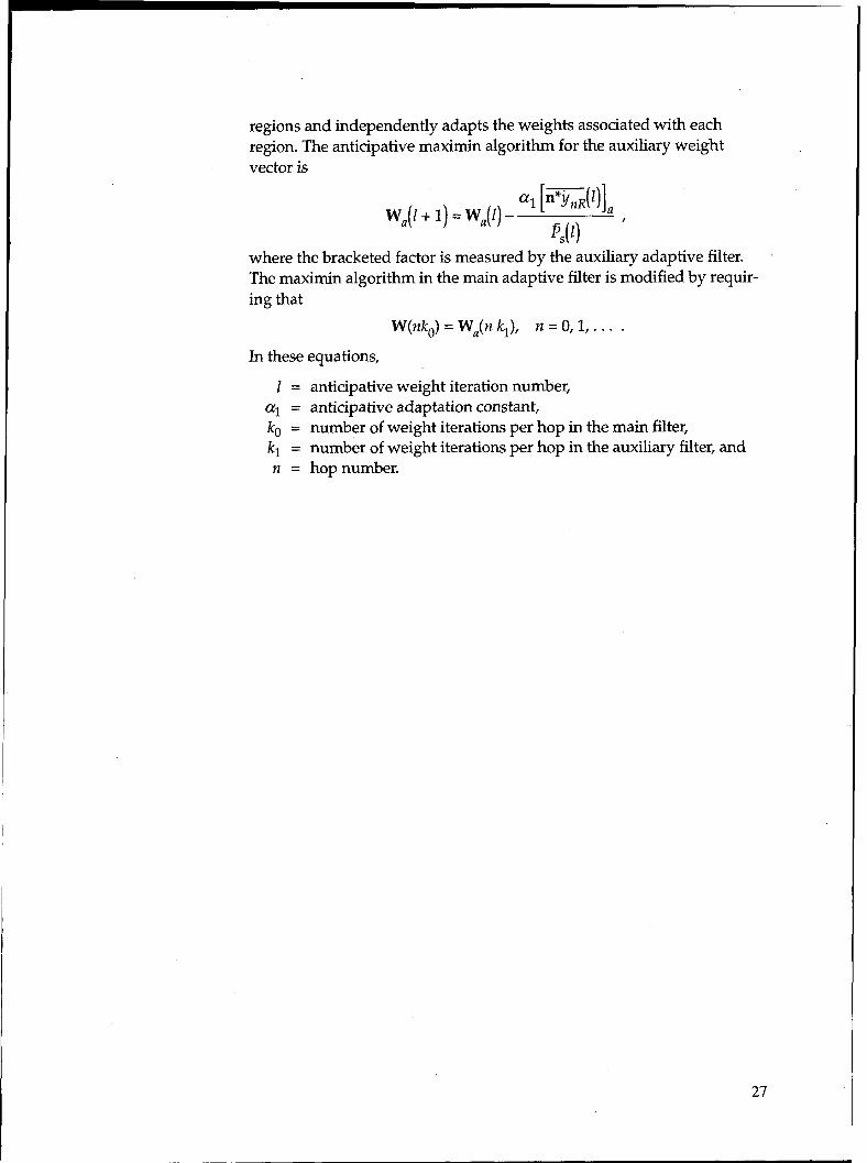
regions and independently adapts the weights associated with each region. The anticipative maximin algorithm for the auxiliary weight vector is

where the bracketed factor is measured by the auxiliary adaptive filter. The maximin algorithm in the main adaptive filter is modified by requir- ing that

W(nQ = W,(n k,), n = 0, 1, . . . .

In these equations,

I= anticipative weight iteration number, al = anticipative adaptation constant, k. = number of weight iterations per hop in the main filter, kl = number of weight iterations per hop in the auxiliary filter, and n= hop number.

27

References

1. K. Bakhru and D. Torrieri, “The maximin algorithm for adaptive arrays and frequency-hopping communications,” IEEE Trans. Antenna Prupug.,

vol. 32, pp. 919-928, September 1984.

2. D. Torrieri and K. Bakhru, “Frequency compensation in an adaptive antenna system for frequency-hopping communications,” IEEE Trans. Aerosp. Electron. Syst., vol. 23, pp. 448467, July 1987.

3. D. Torrieri and K. Bakhru, “An anticipative adaptive array for frequency- hopping communications,” IEEE Trans. Aerosp. Electron. Syst., vol. 24,

pp. 449457, July 1988.

4. D. Torrieri, Principles of Secure Communication Systems, 2nd ed. Boston: Artech House, 1992.

5. J. G. Proakis, Digitid Communicutions, 3rd ed. New York: McGraw-Hill, 1995.

6. R. T. Compton, Adaptive Antennas: Concepfs and Performance. New York: Prentice-Hall, 1988.

7. B. Porat, A Course in Digitd Signal Processing. New York: Wiley, 1997.

8. D. Torrieri and K. Bakhru, “The Effects of Nonuniform and Correlated Noise on Superresolution Algorithms,” IEEE Trans. Antennas Propag., vol. 45, pp. 1214-1218, August 1997.

28

Distribution

Admnstr Telcordia Technologies, Inc. Defns Tech1 Info Ctr Advanced Wireless Technologies Research Attn DTIC-OCP Attn J Liberti 8725 John J Kingman Rd Ste 0944 331 Newman Springs Rd ET Belvoir VA 22060-6218 Red Bank NJ 07701

Cubic Defense Systems Attn K Bakhru (25 copies) 9323 Balboa Avenue San Diego CA 92123

University of Maryland Dept. of Electrical Engineering Attn E Geraniotis College Park MD 20742

Motorola SSTG Attn MS H1175 S Chuprun (4 copies) 8201 E. McDowell Rd Scottsdale AZ 85352

US Army Rsrch Lab Attn AMSRL-CI-AS Mail & Records Mgmt Attn AMSRL-CI-AT Techl Pub (3 copies) Attn AMSRL-CI-LL Techl Lib (3 copies) Attn AMSRL-IS J D Gantt Attn AMSRL-IS-TA J Gowens Attn AMSRL-IS-TP D Torrieri (25 copies) Attn AMSRL-IS-TP R Tobin Adelphi MD 20783-1197

29

REPORT DOCUMENTATION PAGE Form Approved OMB No. 0704-0188

Public reporling burden for this collection of information is estimated to average 1 hour per response. including the time for revi?ving instructiory yching existing data sources, gathering and maintaining the data needed, and completing and reviewing the collection of information. Send COmments regarding this burden estjmate Or any Other aspect Of the- collection of information, including suggestions for reducing this burden, to Washington Headquarters Services. Directorate for fn!OnatlOn OPWatlOnS a?d Rep06 1215 Jefferson Davis Highway, Suite 1204, Arlington, VA 22202.4302, and to the Office of Management and Budget. PapewOlk Reduction PrOleCt (0704.0188). WashIngtOn. DC 20503.

. AGENCY USE ONLY (Leave blank) 2. REPORT DATE 3. REPORT TYPE AND DATES COVERED

December 1999 Final, FY99

,.TITLEANDSUBTITLE The Maximin Algorithm for Adaptive Arrays and 5. FUNDING NUMBERS

Frequency-Hopping Systems DA PR: NA

PE: NA

i. AUTHOR(S) Don Torrieri (ARL), Kesh Bakhru (Cubic Defense Systems)

‘. PERFORMING ORGANIZATION NAME(S) AND ADDRESS

U.S. Army Research Laboratory Attn: AMSRL-IS-T email: [email protected] 2800 Powder Mill Road Adelphi, MD 20783-1197

8. PERFORMING ORGANIZATION REPORT NUMBER

ARL-TR-2026

8. SPONSORINGiMONITORING AGENCY NAME(S) AND ADDRESS

U.S. Army Research Laboratory 2800 Powder Mill Road Adelphi, MD 20783-1197

10. SPONSORlNGlMONlTORlNG AGENCY REPORT NUMBER

1. SUPPLEMENTARY NOTES

ARL I’R: NA AMS code: NA

12a. DlSTRlBUTlONlAVAlLAEIlLtTY STATEMENT Approved for public release; 12b. DlSTRlBUTlON CODE

distribution unlimited.

i3. ABSTRACT (Maximum 200 words)

The maximin algorithm adapts the weights of an antenna array to provide simultaneous interference suppression and beamforming in a frequency-hopping communication system. The algorithm is derived and a digital implementation is presented. Simulation experiments illustrate the ability of the maximin algorithm to rapidly form deep nulls in the directions of interference sources. For the full exploitation of an adaptive array for wideband frequency-hopping communications, some form of frequency compensation is necessary. The strengths, limitations, and variations of three methods are examined.

14. SUBJECT TERMS

Adaptive arrays, frequency hopping, maximin algorithm 15. NUMBER OF PAGES

37 16. PRICE CODE

7. SECURIN CLASSIFICATION OF REPORT

Unclassified

18. SECURITY CLASSIFICATION OF THIS PAGE

Unclassified

19. SECURITY CLASSIFICATION OF ABSTRACT

Unclassified

20. LlYlTATlON OF ABSTRACT

UL

Documents

The Maximin Algorithm for Adaptive Arr&s and … · and the limitations of the maximin algorithm. . . . 111 . Contents Preface