Embed Size (px)
Citation preview

The Market of Medical Office Buildings
by
Yu-Hua Wei
M.Arch., Architecture, 2001 University of Pennsylvania
& B. Arch., Architecture, 1999
Tamkang University
Submitted to the Program in Real Estate Development in Conjunction with the Center for Real Estate in Partial Fulfillment of the Requirements for the Degree of Master of Science in Real Estate Development
at the
Massachusetts Institute of Technology
September, 2012
©2012 Yu-Hua Wei All rights reserved
The author hereby grants to MIT permission to reproduce and to distribute publicly paper and electronic copies of
this thesis document in whole or in part in any medium now known or hereafter created.
Signature of Author_________________________________________________________
Center for Real Estate Yu-Hua Wei
July 30, 2012
Certified by _______________________________________________________________ William C. Wheaton Professor of Economics Thesis Supervisor
Accepted by ______________________________________________________________ David Geltner
Chair, MSRED Committee, Interdepartmental Degree Program in Real Estate Development


The Market of Medical Office Buildings
by
Yu-Hua Wei
Submitted to the Program in Real Estate Development in Conjunction with the Center
for Real Estate on July 30, 2012 in Partial Fulfillment of the Requirements for the Degree of Master of Science in Real Estate Development
ABSTRACT This paper is to define the demand and supply factors and to develop a system to forecast the future development of medical office buildings. At this juncture of time when the health care industry is facing historical changes due to demographic shift, economic challenges and legislative moves, understanding the market mechanism of medical office buildings that provide easy accesses for medical service to aging population, carry lower costs for health care system, and promote the preventive care in medical practices has never been more critical. Medical office buildings as a real estate product type have unique market and development mechanism. They house medical services and have commercial and retail real estate characteristics. To understand the demand and supply of medical office buildings, health care industry that provide medical services, population consuming medical services and real estate industry develop and manage the physical space need to be observed. By using panel regression to analyze historical economic, population and health care employment data across metropolitan areas, we can establish a system that explains the medical office building market. We further quantify the future medical office building demand based on the forecasted economic data and the model established in this paper. The future development of medical office buildings is intricately tied to many factors including the trends predicating the scale and speed of the development. Using the historical events as guidelines and the system established, this paper presents positive outcomes for the demand of medical office buildings under different scenarios. Thesis Supervisor: William C. Wheaton Title: Professor of Economics


Acknowledgment
So many people have helped me to tackle this seemly insurmountable task, and guided me through the process patiently. A simple thank you cannot express my gratitude enough. These people would not have accepted anything more because they are genuinely generous with their knowledge. I would like to thank Sheharyar Bokhar, Lauren Lambie-Hanson and Chunil Kim for sharing their expertise on data processing; I would like to thank Alfonzo Leon, Matt Assia and Walter Markowitz for providing their insights on the health care real estate industry; and to thank many who extended their helping hands without even knowing me in person. I am fortunate enough to have people who helped me, even more fortunate to have people who supported me. The supports coming from their loving and encouraging natures comforted and invigorated me, and got me through the most unproductive moments. I would like to thank the people who endured my shortness and cynicism at times and still managed to care for me. Most importantly, I would like to thank Prof. Wheaton who guided and taught with such grace and acute sentiment. He taught me that pursue of knowledge is a never ending quest; however, with the right information and tools, people can perhaps learn and grow to know a little bit more about this world.


|Table of Contents 7
Contents Chapter 1. Introduction ........................................................................................................................................... 13
1.1 Research Motivation ..................................................................................................................................... 13
1.2 Background.................................................................................................................................................... 14
1.3 Research Methodology ................................................................................................................................. 16
1.4 Summary Conclusion ..................................................................................................................................... 16
1.5 Thesis Structure ............................................................................................................................................. 17
Chapter 2. Literature review ................................................................................................................................... 19
2.1 Definition ....................................................................................................................................................... 19
2.2 Health Care Market ....................................................................................................................................... 19
2.2.1 Aging and Health Care Spending ........................................................................................................... 19
2.2.2 Aging and Medical Services ................................................................................................................... 21
3.2.3 Medical Service Supply ............................................................................................................................... 21
2.3 MOB Market .................................................................................................................................................. 23
2.3.1 Development Mechanism ...................................................................................................................... 23
2.3.2 Ownership .............................................................................................................................................. 24
2.3.3 Capital Market ....................................................................................................................................... 24
2.4 Future Changes.............................................................................................................................................. 25
2.4.1 Health Care Employment Under New Regulation ................................................................................. 26
2.4.2 MOB Market .......................................................................................................................................... 27
2.4.3 Chapter Summary .......................................................................................................................................... 28
Chapter 3. Methodology and Data .......................................................................................................................... 29
3.1 Definition ....................................................................................................................................................... 29
3.1 The Data ........................................................................................................................................................ 29
3.1 Preform panel data analysis .......................................................................................................................... 31
3.2 Forecasts for MOB ......................................................................................................................................... 35
3.3 Chapter Summary .......................................................................................................................................... 35
Chapter 4. Relevant Economic Data Analysis .......................................................................................................... 37
4.1 Introduction................................................................................................................................................... 37
4.2 Demographic, Employment and Income ....................................................................................................... 38
4.2.1 Aging Trend ............................................................................................................................................ 39
4.2.2 Employment and Income Trend ............................................................................................................ 42

8 Table of Contents |
4.3 Health Care Employment and MOB ................................................................................................................ 44
4.3.1 Health Care Practice Trends in Total ........................................................................................................ 44
4.3.2 Health Care Practice Trends in Each MSA ................................................................................................ 45
4.4 Health Care Employment and MOB Trend .................................................................................................... 47
4.5 Chapter Summary .......................................................................................................................................... 48
Chapter 5. Medical Office Building Model .............................................................................................................. 49
5.1 Definition ....................................................................................................................................................... 49
5.2 Top‐Tier: MOB model .................................................................................................................................... 49
5.3 Base‐Tier: Health Care Employment Models ................................................................................................ 53
5.3.1 Offices of Physicians .............................................................................................................................. 53
5.3.2 Offices of Dentists .................................................................................................................................. 56
5.3.3 Offices of Others .................................................................................................................................... 58
5.3.5 Outpatient Care Centers ........................................................................................................................ 60
5.3.6 Medical and Diagnostic Laboratories .................................................................................................... 62
5.3.7 General Medical and Surgical Hospital .................................................................................................. 64
5.3.9 Independent Variables for Health Care Employment ............................................................................ 66
5.4 Chapter Summary .......................................................................................................................................... 67
Chapter 6. Forecasts ................................................................................................................................................ 69
6.1 Definition ....................................................................................................................................................... 69
6.2 Forecast for Health Care Employment .......................................................................................................... 70
6.2.1 Office of Physicians ................................................................................................................................ 71
6.2.2 Office of Dentists ................................................................................................................................... 72
6.2.3 Office of Others ..................................................................................................................................... 75
6.2.4 Outpatient Care Centers ........................................................................................................................ 77
6.2.5 Medical and Diagnostic Laboratories .................................................................................................... 79
6.2.6 General Medical and Surgical Hospitals ................................................................................................ 81
6.2.7 Health Care Employment in 2022 .......................................................................................................... 83
............................................................................................................................................................................. 83
6.3 Forecasts for Medical Office Building ............................................................................................................ 88
6.3.1 MOB Trend ............................................................................................................................................. 88
6.3.2 MOB in 2022 .......................................................................................................................................... 89
6.3 Chapter Summary .............................................................................................................................................. 93
Chapter 7. Conclusion.............................................................................................................................................. 97
Bibliography ............................................................................................................................................................... 103

|Table of Contents 9
Appendix A................................................................................................................................................................. 105
Appendix B ................................................................................................................................................................. 106
Appendix C ................................................................................................................................................................. 107
Appendix D ................................................................................................................................................................ 108
Appendix E ................................................................................................................................................................. 112
Appendix F ................................................................................................................................................................. 113
Appendix G ................................................................................................................................................................ 115
Appendix H1 .............................................................................................................................................................. 116
Appendix H2 .............................................................................................................................................................. 118
Appendix H3 .............................................................................................................................................................. 120
Appendix H4 .............................................................................................................................................................. 122
Appendix H5 .............................................................................................................................................................. 124
Appendix H6 .............................................................................................................................................................. 126
Appendix I .................................................................................................................................................................. 128
APPENDIX J ................................................................................................................................................................ 129
Appendix K ................................................................................................................................................................. 131
Appendix L1 ............................................................................................................................................................... 133
Appendix L2 ............................................................................................................................................................... 135
Appendix L3 ............................................................................................................................................................... 137
Appendix L4 ............................................................................................................................................................... 139
10 Table of Contents |
FIGURES Figure 1‐1 MOB Market ............................................................................................................................................... 15
Figure 2‐1: Annual Rates Of Physician Office Visits And Rates Of Visits With Medications Prescribed Or Continued:
National Ambulatory Medical Care Survey, 1998 And 2008 ....................................................................................... 19
Figure 2‐2: Percent Distribution Of Population And Physician Office Visits: United State, 1998 And 2008 ................ 19
Figure 2‐3: Inpatient Vs Outpatient Surgery Volume 19981‐2005 .............................................................................. 20
Figure 2‐4: MOB Cape Rate And Per Square Footage Sale Price ................................................................................. 23
Figure 2‐5: National Health Expenditure Growth Index .............................................................................................. 24
Figure 2‐6: MOB Trading Volume ................................................................................................................................ 25
Figure 4‐1: Employment, Population, Income, Health Care Employment And Mob Growth Index ............................ 36
Figure 4‐2: Population Composition ............................................................................................................................ 37
Figure 4‐3: Population Changes, 1988‐2011 ................................................................................................................ 39
Figure 4‐4: Population Changes, 2011‐2022 ................................................................................................................ 39
Figure 4‐5: Age Groups Fractional Changes, 1988‐2011 ............................................................................................. 40
Figure 4‐6: Age Groups Fractional Changes, 2011‐2022 ............................................................................................. 40
Figure 4‐7: Percentage Change In Employment Per Captia, 1988‐2011 ...................................................................... 41
Figure 4‐8: Percentage Change In Employment Per Capita, 2011‐2022 ...................................................................... 41
Figure 4‐9: Percentage Change In Income Per Captia, 1988‐2011 .............................................................................. 41
Figure 4‐10: Percentage Change In Income Per Captia, 2011‐2022 ............................................................................ 41
Figure 4‐11: Health Care Employment Composition ................................................................................................... 42
Figure 4‐12: Sectional Health Care Growth Index ....................................................................................................... 43
Figure 4‐13: Fractional Changes In Health Care Employment Sectios, 1988‐2011 ...................................................... 44
Figure 4‐14: Healht Care Employment And Mob Growth Rate ................................................................................... 45
Figure 5‐1: Weighted Influences For MOB .................................................................................................................. 49
Figure 5‐2: Lnphy Time Variables ................................................................................................................................ 53
Figure 5‐3: Lindent Time Variables .............................................................................................................................. 55
Figure 5‐4: Lnothers Time Variables ............................................................................................................................ 57
Figure 5‐5: Lnout Time Variables ................................................................................................................................ 59
Figure 5‐6: Inlabs Time Variables ................................................................................................................................. 61
Figure 5‐7: Lnhosp Time Variables ............................................................................................................................... 63
Figure 5‐8: Coefficients For HC Emply Independent Variables .................................................................................... 64
Figure 5‐9: Coefficient For Time Variables Of HC Emply Models ................................................................................. 65
Figure 6‐1: Offices Of Physicians In 2022 ..................................................................................................................... 69
Figure 6‐2: Lnphy Time Variables ................................................................................................................................ 69
Figure 6‐3: Office Of Physicians In Continuous And Slow Growth In 2022 .................................................................. 70
Figure 6‐4: Offices Of Dentists ..................................................................................................................................... 71
Figure 6‐5 : Lndent Time Variables .............................................................................................................................. 71
Figure 6‐6: Lndent Time Variables ............................................................................................................................... 71
Figure 6‐7: Office Of Other Health Practitioners In 2022 ............................................................................................ 73
Figure 6‐8: Lnothers Time Variables ............................................................................................................................ 73
Figure 6‐9: Office Of Other Health Practitioners In Continuous And Slow Growth ..................................................... 74
Figure 6‐10: Outpatient Care Centers In 2022 ............................................................................................................. 75
Figure 6‐11: Lnout Time Variables ............................................................................................................................... 75

|Table of Contents 11
Figure 6‐12: Outpatient Care Centers .......................................................................................................................... 76
Figure 6‐13: Medical And Diagnostic Laboratories In 2022 ......................................................................................... 77
Figure 6‐14: Lnlab Time Variables ............................................................................................................................... 77
Figure 6‐15: Medical And Diagnostic Laboratories ...................................................................................................... 78
Figure 6‐16: Medical And Surgical Hospital Employment In 2022 ............................................................................... 79
Figure 6‐17: Lnhosp Time Variables ............................................................................................................................. 79
Figure 6‐18: General Medical And Surgical Hospital Employment Continuous And Slow Trends ............................... 80
Figure 6‐19: Income, Employment, Population And Health Care Growth Index ......................................................... 81
Figure 6‐20:Healh Care Employment 2022 .................................................................................................................. 82
Figure 6‐21:Health Care Employment Composition .................................................................................................... 83
Figure 6‐22: Fractional Changes In Health Care Employment, Continuous Trend 2011‐2022 .................................... 84
Figure 6‐23: Fractional Changes In Health Care Employment, Slow Trend 2011‐2022 ............................................... 85
Figure 6‐24: Mob Time Variables ................................................................................................................................. 86
Figure 6‐25: 2022 MOB Stock – Scenario 1 .................................................................................................................. 87
Figure 6‐26: MOB Changes And Growth Rates‐Scenario 1 .......................................................................................... 88
Figure 6‐27: 2022 MOB Stock – Scenario 2 .................................................................................................................. 89
Figure 6‐28: MOB Changes And Growth Rates – Scenario 2 ....................................................................................... 90
Figure 6‐29: 2022 MOB Stock – Scenario 3 .................................................................................................................. 91
Figure 6‐30: MOB Growth Rates – 3 Scenarios ............................................................................................................ 94
Figure 6‐31: MOB In 2022 – 3 Scenarios ...................................................................................................................... 94
Figure 7‐1: Ranking For MOB Growth Rate ................................................................................................................. 97
Figure 7‐2: Ranking For MOB Square Footage Increases ............................................................................................. 98
TABLES Table 2‐1: Top‐Tier Model: MOB ................................................................................................................................. 17
Table 2‐2: Base‐Tier Model: Health Care Employment ............................................................................................... 18
Table 2‐3: Location Vriables MSA ................................................................................................................................ 19
Table 2‐4: Naica Assocation Section 62 ....................................................................................................................... 20
Table 3‐1: Personal Health Care Spending Per Capita ................................................................................................. 24
Table 3‐2: Per Person Spending And Annual Percnetage Change 1963‐2000 ............................................................. 24
Table 5‐1: MOB Regression Result............................................................................................................................... 46
Table 5‐2: Inphy Regression Result .............................................................................................................................. 49
Table 5‐3: Indent Regression Result ............................................................................................................................ 51
Table 5‐4: Inothers Regression Result ......................................................................................................................... 53
Table 5‐5: Inoutpat Regression Result ......................................................................................................................... 55
Table 5‐6: Inlabs Regression Result ............................................................................................................................. 57
Table 5‐7: Inhosp Regression Result ............................................................................................................................ 59
Table 6‐1: MOB Stock .................................................................................................................................................. 88

12 Table of Contents |
(This page is intentionally blank)
Chapter 1 | Introduction 13
Chapter 1. INTRODUCTION
1.1 RESEARCH MOTIVATION
Health care real estate is based on the essential human need for medical services that is
heavily supported by the US government, and protected from the volatility of economic cycles.
Medical office buildings as a specific investment category within health care real estate is with
lower vacancy rates and less volatile cap rate compare to other commercial real estate. They
house out‐patient services that can be physically separated from hospital campus, and have
unique market mechanisms for developments. With the foreseeable increase of demand and
supply for out‐patient services, more discussions and interests for medical office building
investment and development have been generated.
For the demand for medical services, the general demographic trend needs to be
observed. The US population is aging. The population of elderly citizens has been increasing in
number and becoming a larger percentage. The current 45‐64 age group uses the most of the
medical resources because of its share of population and the use of medical services, the age
group of over 65 has the most intense use for medical services. In the near future, the current
large 45‐64 age group will enter the over 65 age group, and the medical services need
demanded by both larger elderly population and higher density will grow exponentially. The
demand of medical services due to aging is not only increasing but also becoming more
concentrated on out‐patient services.
Hospitals and health care systems have incorporated such trends into their practices,
and expanded out‐patient services. Changes in medical service delivery affect the supply of out‐
patient services in addition to the increasing demand driven by demographic shifts. Such
changes include increasing availability of treatments and procedures facilitated by technological
advancement, and the decreasing carrying cost encouraged by regulatory incentives. For the
same reason, more physician practice groups were able to start or expand their practices and
introduce more supply in out‐patient services.
14 Introduction | Chapter 1
The increasing demand and supply for out‐patient services can explain the enlarging
market for medical office buildings, but the unique development mechanism creates a special
profile for such market. The physical characteristics of medical office buildings play a crucial
role in the overall commerce strategy for owners and operators. Medical office buildings that
can be located independently from main campuses at convenient locations can provide easy
accesses to patients and physically expand hospital networks. In addition to physical
characteristics, medical office buildings as real estate properties can act as vehicles for hospitals
and physicians to build mutually beneficial relationships, or as investment opportunities to
many. Hospitals and healthcare systems sometimes help physicians to set up private practices
in medical office buildings on or off campuses to increase physicians’ income.1 By strategically
locating such practices, hospital and health care systems can retain the talent and broaden
referral networks to stay competitive.
It is critical to understand which factors in the supply, demand and development
mechanism is the most influential. This thesis is to analysis the market factors described earlier,
and attempt to explain the relationship among these factors using regression models based on
the historical data. Combining the data analysis and observation for future changes, we can
identify where opportunities are and what risks are involved.
1.2 BACKGROUND
Medical office buildings (MOB) are facilities constructed for medical use and provide
out‐patient medical services related spaces. These include medical professional office buildings,
ambulatory care facilities, surgery centers, ambulatory surgical centers, medical imaging
facilities, outpatient care facilities and wellness centers. Opposite to in‐patient service facilities
providing over‐night stay for patients measured in number of beds, out‐patient service facilities
are measured in square footage conventionally. All medical service facilities stated are included
in MOB stock data in square footage presented in this paper.
1 Cain Brothers, “Physician Ownership Participation in Medical Office Buildings,” Strategies in Capital Finance, Volume 51 (July 2006)

Chapter 1 | Introduction 15
MOB as health care real estate differs from hospitals, and it can be developed and
operated by different organizations. In addition to hospitals and health care systems, physician
practice groups, developers and institutional investors can also be the owners, buyers and
operators in the MOB market. Different ownership structures have been developed to reflect
the regulatory changes and capital market trends, and thus facilitate the MOB market liquidity
and investment interests.
On the tenant side, the inelasticity of the medical service demand reinforces the
steadiness of the medical related practices occupying MOBs. These practices include
professional private entities such as physicians and dentists, independent or codependent
laboratories processing medical samples and others such as imagining suites and surgical
centers affiliated with hospitals and health care systems providing out‐patient medical related
services. Following the general trend of medical service demands, these practices have been
expanding regardless of economic cycles. Adding to the business demand, the physical
specifications needed to each of the specific function and operation limit the flexibility to move
these facilities. These result the low turn‐over and vacancy rate for MOBs in general.
According to the industry analysis from Stifel Nicolaus, MOB comprised 62 % of total
health care real estate value in 2008. The majority of the MOB market is owned and operated
by providers such as hospitals, health care systems and physician owned practices, and the
transition from health care providers to institutional investors has been very gradual2. The
empirical evidence for such phenomenon is also in the low transition volume for MOB3. The
capital market influences on MOB market have been increasing. The capital market force for
future development could play a bigger role because the increasing interests in investment in
MOB and pressure for the efficiency of the provider will open the market to more institutional
investers2.
2 Bernstein, Daniel and Doctrow, Jerry. “Healthcare REITS: Antidote for an Economic Downturn?” Stifel Nicolaus Equity Research Industry Analysis (Winter 2008) 3 Shilling, Gary. “The Outlook for Health Care.” Urban Land Institute, (2011)

16 Introduction | Chapter 1
1.3 RESEARCH METHODOLOGY
In order to find development and investment opportunities, understand differences of
markets, and study the implication of policy changes associated with health care practices, the
relationships among the factors of supply and demand for MOB development based on the
demographic and economic data need to be analyzed and constructed.
Two‐tier model needs to be established for MOB model. Base‐tier model is to use the
demographic and economic data as independent variables to explain the health care
employment by each of the sector that occupies MOB spaces. Top‐tier model is to analyze the
relationship between sectors of health care employment as independent variables for MOB
stocks. Both models are established based on the panel data arranged across twenty‐three
years and 63 MSAs. With the fixed‐effect regression, we can exam the relationship among
independent variables and dependent variable cross‐time and markets.
Once the two‐tier model is established, with the forecasted demographic and economic
data developed by specialized agency, the sectors of health care employment can be estimated
with the base‐tier models. MOB demand can be generated with the forecasted sectional heath
care employment data with two‐tier model in each of the metropolitan area.
Refer to Chapter 3 for a full description of the methodology and data.
1.4 SUMMARY CONCLUSION
The attempt for this paper is to structure relationships among demand and supply
factors that weaved into demographic changes, health care practice, political issues, real estate
market for MOB. We identify the market factors of users, tenants and owners for MOB, and
study what influences for these factors. These influences include health care insurance, health
care regulation and capital market policy captured in the historical economic and health care
employment data will be analyzed and quantified in the data analysis. We organize these
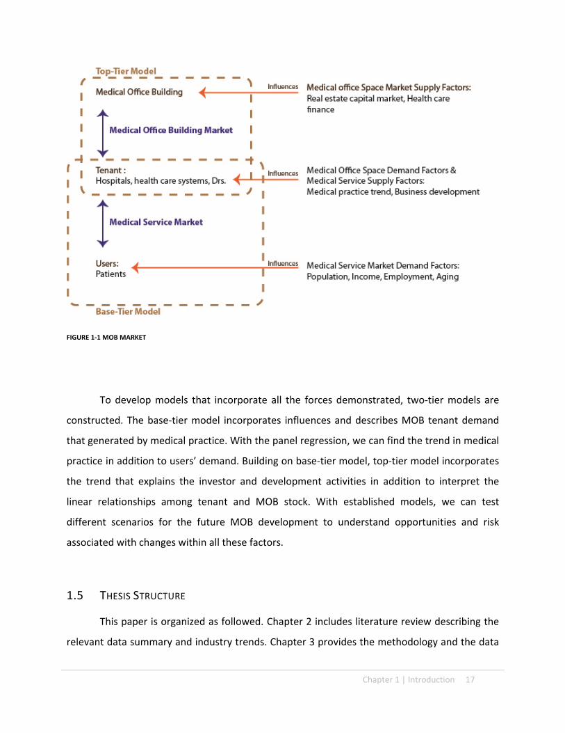
factors and influences in Figure 1‐1, and conclude the data analysis with MOB model. We
incorporate possible changes and provide the MOB demand in quantity.
Chapter 1 | Introduction 17
FIGURE 1‐1 MOB MARKET
To develop models that incorporate all the forces demonstrated, two‐tier models are
constructed. The base‐tier model incorporates influences and describes MOB tenant demand
that generated by medical practice. With the panel regression, we can find the trend in medical
practice in addition to users’ demand. Building on base‐tier model, top‐tier model incorporates
the trend that explains the investor and development activities in addition to interpret the
linear relationships among tenant and MOB stock. With established models, we can test
different scenarios for the future MOB development to understand opportunities and risk
associated with changes within all these factors.
1.5 THESIS STRUCTURE
This paper is organized as followed. Chapter 2 includes literature review describing the
relevant data summary and industry trends. Chapter 3 provides the methodology and the data

18 Introduction | Chapter 1
information. Chapter 4 will be the general observation and analysis of the data, and regression
results for health care industry trend and MOB model will be presented in Chapter 5.
Chapter 6 will be the forecast of MOB based on the forecasted health care employment
information established in tier one model. Conclusions for MOB markets will be presented in
Chapter 7.

Chapter 2 | Literature review 19
Chapter 2. LITERATURE REVIEW
2.1 DEFINITION
As stated in previous chapter, the main purpose of this Chapter is to review the research
paper, studies and relevant statics summaries in order to define the relationship between aging
and health care usage. Many studies also indicate that health care practice changes not only
because of the aging population, but also the health care commerce. We review industry
reports and white papers that discuss how MOB is developed in corresponding to changing
health care practices in the past. Building on the understanding of development mechanism for
MOB, we advance the discussion into what factors are expected to change in corresponding to
future events.
2.2 HEALTH CARE MARKET
The demand for MOB is coming from the demand of medical services, especially
outpatient services. In order to understand how the population consumes outpatient medical
services, we look into medical spending reports and outpatient service surveys to quantify
service demands and trends.
2.2.1 AGING AND HEALTH CARE SPENDING
The fact that elderly requires more medical services is demonstrated in the increasing
health care spending. As Table 2‐1 indicates, the total spending for health care regardless of the
sources of the payment is the highest among the age group older than 65. It amounts almost
three times of the spending for age group 19‐64; age groups in 45‐54 and 55‐64 also have
higher spending per captia comparing to younger groups in 2004.
It is not only the aging that’s contributing to health care spending increases, the study
proves that insurance policies change the pattern of health care spending in different age
groups1 as shown in Table 2‐2. With influences from insurance policies such as enactments of
1 Cutler, David M., Meara, Ellen and White, Chapin. “Trends in Medical Spending By Age, 1963‐2000.” Health Affairs, Volume 23, No. 4 ( July/August, 2004)

20 Literature review | Chapter 2
Medicare and Medicare reform in 1965 and 1999, the medical spending in elderly group has
rapid growth in 1963‐1970 but has declined in 1996‐2000.
Personal Health Care Spending Per Capita (in dollars) Age Group Total
Total Private PHI OOP
Other Private
Total Public Medicare Medicaid
Other Public
Total $5,276 $2,921 $1,898 $802 $221 $2,355 $1,032 $918 $405
0‐18 $2,650 $1,558 $1,096 $338 $124 $1,092 $2 $819 $271
19‐44 $3,370 $2,269 $1,559 $520 $190 $1,100 $87 $662 $351
45‐54 $5,210 $3,760 $2,570 $899 $290 $1,451 $310 $737 $403
55‐64 $7,787 $5,371 $3,784 $1,225 $363 $2,415 $706 $1,026 $683
65‐74 $10,778 $3,851 $2,174 $1,437 $241 $6,927 $5,242 $1,112 $573
75‐84 $16,389 $5,066 $2,428 $2,281 $358 $11,323 $8,675 $2,058 $590
85+ $25,691 $8,304 $2,817 $4,886 $601 $17,387 $10,993 $5,424 $970
0‐18 $2,650 $1,558 $1,096 $338 $124 $1,092 $2 $819 $271
19‐64 $4,511 $3,117 $2,154 $722 $241 $1,395 $239 $738 $417
65+ $14,797 $4,888 $2,351 $2,205 $331 $9,909 $7,242 $2,034 $633
Source: Center for Medicare and Medicaid Studies
TABLE 2‐1: PERSONAL HEALTH CARE SPENDING PER CAPITA
Per Person Spending And Annual Percentage Change In Spending, By Year And Age Group, 1963–2000
Age
Year 0–5 6–64 65–74 75+ All age group
1963 $245 $663 $1,164 $1,928 $684 1970 559 929 2,266 4,381 1,1021977 604 1,160 3,300 7,113 1,5021987 1,195 1,588 6,057 11,513 2,3681996 1,663 2,423 7,219 16,513 3,5002000 1,525 2,888 9,094 15,756 3,962
Annual growth rate (percent)
1963–1970 11.8 4.8 9.5 11.7 6.81970–1987 4.5 3,2 5.8 5.7 4.51987–1996 3.7 4.7 2 4 4.31996–2000 –2.2 4.4 5.8 –1.2 3.11963–2000 4.9 4 5.6 5.7 4.7
SOURCE: Authors’ calculations1. NOTE: Results are presented in inflation‐adjusted July 2002 dollars.
TABLE 2‐2: PER PERSON SPENDING AND ANNUAL PERCNETAGE CHANGE 1963‐2000
Chapter 2 | Literature review 21
2.2.2 AGING AND MEDICAL SERVICES
In National Ambulatory Medical Care Survey in 2007, many conclusions from the
complied data state that 86% of office visits were made to physicians located in metropolitan
statistical areas (MSAs)2 and the visit rate was highest for elderly people 75 years and over.
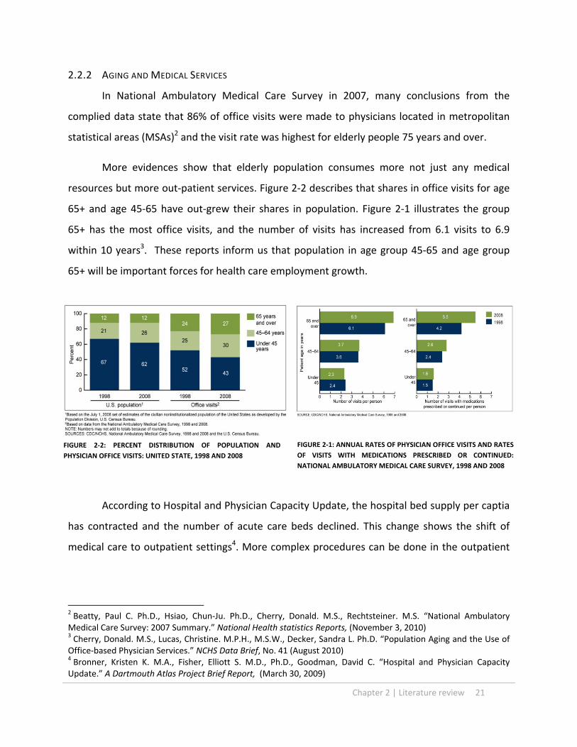
More evidences show that elderly population consumes more not just any medical
resources but more out‐patient services. Figure 2‐2 describes that shares in office visits for age
65+ and age 45‐65 have out‐grew their shares in population. Figure 2‐1 illustrates the group
65+ has the most office visits, and the number of visits has increased from 6.1 visits to 6.9
within 10 years3. These reports inform us that population in age group 45‐65 and age group
65+ will be important forces for health care employment growth.
3.2.3 MEDICAL SERVICE SUPPLY
According to Hospital and Physician Capacity Update, the hospital bed supply per captia
has contracted and the number of acute care beds declined. This change shows the shift of
medical care to outpatient settings4. More complex procedures can be done in the outpatient
2 Beatty, Paul C. Ph.D., Hsiao, Chun‐Ju. Ph.D., Cherry, Donald. M.S., Rechtsteiner. M.S. “National Ambulatory Medical Care Survey: 2007 Summary.” National Health statistics Reports, (November 3, 2010) 3 Cherry, Donald. M.S., Lucas, Christine. M.P.H., M.S.W., Decker, Sandra L. Ph.D. “Population Aging and the Use of Office‐based Physician Services.” NCHS Data Brief, No. 41 (August 2010) 4 Bronner, Kristen K. M.A., Fisher, Elliott S. M.D., Ph.D., Goodman, David C. “Hospital and Physician Capacity Update.” A Dartmouth Atlas Project Brief Report, (March 30, 2009)
FIGURE 2‐2: PERCENT DISTRIBUTION OF POPULATION AND
PHYSICIAN OFFICE VISITS: UNITED STATE, 1998 AND 2008 FIGURE 2‐1: ANNUAL RATES OF PHYSICIAN OFFICE VISITS AND RATES
OF VISITS WITH MEDICATIONS PRESCRIBED OR CONTINUED:
NATIONAL AMBULATORY MEDICAL CARE SURVEY, 1998 AND 2008
22 Literature review | Chapter 2
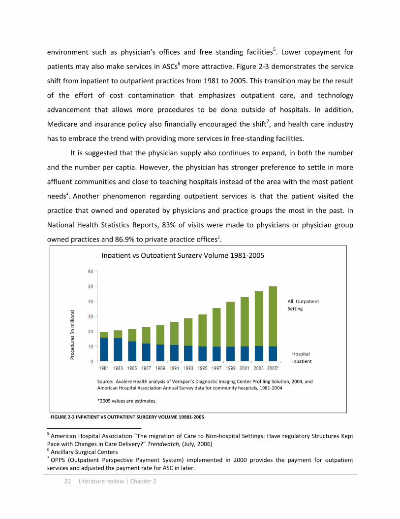
environment such as physician’s offices and free standing facilities5. Lower copayment for
patients may also make services in ASCs6 more attractive. Figure 2‐3 demonstrates the service
shift from inpatient to outpatient practices from 1981 to 2005. This transition may be the result
of the effort of cost contamination that emphasizes outpatient care, and technology
advancement that allows more procedures to be done outside of hospitals. In addition,
Medicare and insurance policy also financially encouraged the shift7, and health care industry
has to embrace the trend with providing more services in free‐standing facilities.
It is suggested that the physician supply also continues to expand, in both the number
and the number per captia. However, the physician has stronger preference to settle in more
affluent communities and close to teaching hospitals instead of the area with the most patient
needs4. Another phenomenon regarding outpatient services is that the patient visited the
practice that owned and operated by physicians and practice groups the most in the past. In
National Health Statistics Reports, 83% of visits were made to physicians or physician group
owned practices and 86.9% to private practice offices2.
5 American Hospital Association “The migration of Care to Non‐hospital Settings: Have regulatory Structures Kept Pace with Changes in Care Delivery?” Trendwatch, (July, 2006) 6 Ancillary Surgical Centers 7 OPPS (Outpatient Perspective Payment System) implemented in 2000 provides the payment for outpatient services and adjusted the payment rate for ASC in later.
Inpatient vs Outpatient Surgery Volume 1981‐2005
Procedures (in m
illions)
All Outpatient
Setting
Hospital
Inpatient
Source: Avalere Health analysis of Verispan’s Diagnostic Imaging Center Profiling Solution, 2004, and American Hospital Association Annual Survey data for community hospitals, 1981‐2004
*2005 values are estimates.
FIGURE 2‐3 INPATIENT VS OUTPATIENT SURGERY VOLUME 19981‐2005

Chapter 2 | Literature review 23
2.3 MOB MARKET
MOB is predicated not just by the space market servicing medical activities, it is also a
real estate product influenced by the real estate capital market. With the understanding of the
expanding health care industry and the demand for outpatient services, we want to understand
how the parties interested in MOB developments respond to such demand. Many hospitals and
health care real estate developers and investors have to be fully aware of the financial
implications for planning, developing, managing and trading MOB in responding to the ever
changing markets in health care and real estate industries.
2.3.1 DEVELOPMENT MECHANISM
Hospitals have expanded their outpatient services with MOB or other ancillary facilities.
Reasons for hospitals to develop MOB are not only for expanding their outpatient services, but
also maintain their relationship with physicians8. Hospitals have provided the equity joint
venture opportunities for physicians for MOB9 as a part of economic integration arrangements,
and this will also expand hospital’s network. However, hospitals need consider how MOBs as
assets presented in their balance sheet before and after the construction. MOB that’s not
classified as hospital facilities could trigger many accounting and rating issues for hospitals10.
Physicians also participated in the development in MOB to generate additional income.
The participation allows physicians to develop and control their practice spaces, and add real
estate investment into their portfolio. Such practice is not new, the trend, however, is shifting
toward back to hospital owning the facility with third party developer or manager11 because the
increasing capital requirement and complexity of the development process, in addition to legal
concerns commend more sophisticated development knowledge.
8 Burns, Lawton Robert., Muller, Ralph W. “Hospital‐Physician Collaboration: Landscape of Economic Integration and Impact on Clinical Integration.” The Milbank Quarterly, Vol. 86, No. 3 (2008) 9 In this paper, we include all ancillary surgical centers, outpatient care centers and medical and diagnostic laboratories in MOB stock. 10 Cain Brothers. “Physician Ownership Participation in Medical Office Buildings.” Strategies in Capital Finance, Vol. 51 (July 2006) 11 Cain Brothers. “Medical Real Estate: Trend in Third Party Development—From Niche to Mainstream” Strategies in Capital Finance, Vol. 46 (July 2005)
24 Literature review | Chapter 2
Third party developers/owner provide many benefits for hospitals and physicians with
regard the MOB development, which include providing expertise in leasing, managing tenant
and hospital relationships, managing operation and eliminate legal risks. Also, the third party
developer can provide capitals and efficiency in development, while many hospitals do not have
such capacities in house and have higher cost of capitals.
2.3.2 OWNERSHIP
MOB could be developed with these options: in‐house owner development, fee‐based
developers and third party developer/owner options. The in‐house owner development and
fee‐based developer options are with single ownership. With the third party developer/owner,
hospital will entry into a ground lease or burn‐off lease with developer to maintain certain type
of control and flexibility11.
After the development phase, many types of ownership structure can apply to owing
MOB. The hospitals could own the asset 100 %, sell off the property to third‐party and operate
under the third‐party owner, or sale of property to joint venture while maintaining an
ownership position 12 . Each of the ownership strategies has its own advantages and
disadvantages, and key issues for considerations are the owner’s control over the property,
relationship with tenants, regulatory issues and the use of equity.
2.3.3 CAPITAL MARKET
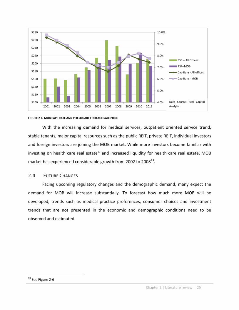
The cash flow returns from well‐managed medical properties can be more stable than
typical commercial real estate investment. Doctors as tenants for MOB typically have longer
lease and lower turnover level than other type of office tenants; and MOBs under master leases
with hospitals as credit tenants are even more stable. Looking at the recent sale price per
square footage, and the cap rate for MOB as shown in Figure 2‐4, the sale per square foot have
surpassed other offices after the recession, and the cap rat become less volatile compare to
offices’ in recent years. Some consider MOB good investment against inflation because of
health care market’s character and robust government support.
12 Cain Brothers. “From Strategic Assets to Tactical Investments: Changing Attitudes Toward Medical Office Building Ownership.” Strategies in Capital Finance, Vol. 41 (Summer 2003)
Chapter 2 | Literature review 25
FIGURE 2‐4: MOB CAPE RATE AND PER SQUARE FOOTAGE SALE PRICE
With the increasing demand for medical services, outpatient oriented service trend,
stable tenants, major capital resources such as the public REIT, private REIT, individual investors
and foreign investors are joining the MOB market. While more investors become familiar with
investing on health care real estate10 and increased liquidity for health care real estate, MOB
market has experienced considerable growth from 2002 to 200813.
2.4 FUTURE CHANGES
Facing upcoming regulatory changes and the demographic demand, many expect the
demand for MOB will increase substantially. To forecast how much more MOB will be
developed, trends such as medical practice preferences, consumer choices and investment
trends that are not presented in the economic and demographic conditions need to be
observed and estimated.
13 See Figure 2‐6
4.0%
5.0%
6.0%
7.0%
8.0%
9.0%
10.0%
$100
$120
$140
$160
$180
$200
$220
$240
$260
$280
2001 2002 2003 2004 2005 2006 2007 2008 2009 2010 2011
PSF ‐‐ All Offices
PSF‐‐MOB
Cap Rate ‐ All offices
Cap Rate ‐ MOB
Data Source: Real Capital
Analytic

26 Literature review | Chapter 2
2.4.1 HEALTH CARE EMPLOYMENT UNDER NEW REGULATION
Health care industry had responded differently to major regulatory changes in the past,
and the implication for future changes is unknown. The US government estimated additional 32
million will be covered by the extended insurance, and the health care reform will focus on the
preventive care and the cost control. With these goals built into the legislation, many cost
savings and additional expanses in health care expense have been projected. The projection of
the national health care expenditures with and without “Patient Protection and Accountable
Care Act” from 2010 to 2019 is indicating the continuous growth in health care spending. The
Figure 2‐5 compiled from the data14 describes that with the expanded health care coverage as
well as the increased efficiency for medical practices, the growth of health care spending will
initially be slower but surpass the original projection in years after, although not in a great scale.
The contradicting arguments of the need of greater health care services and the
shortage of health care employee rise questions concerning how and how much health care
industry will be growing, but the fact that the health care industry needs to grow to respond to
14 See Appendix A
1
1.02
1.04
1.06
1.08
1.1
1.12
1.14
1.16
1.18
1.2
2010 2011 2012 2013 2014 2015 2016 2017 2018 2019
National Health Expenditures as Percentage of GDP Growth Index
Without PPACA With PPACA
Data Source: Center of Medicare and Medicaid, Office of Actuary
FIGURE 2‐5: NATIONAL HEALTH EXPENDITURE GROWTH INDEX

Chapter 2 | Literature review 27
essential human medical service needs suggests that the growing trend is likely to be sustained
through many government incentives.
2.4.2 MOB MARKET
MOB provides many answers to upcoming challenges for health care industry. It is still,
however, a real estate product that ties to the broader real estate market. The recent decline of
real estate market has impacted MOB market in spite of the inelastic demand for health care
services. The vacancy rate for MOB was at 10 to 12 % in 2010, and it will require certain time
for the market to consolidate the empty spaces15. Great amount of over built commercial space
during mid‐2000s’ will also likely to slow down the MOB development. Examples such as new
development adopting and renovating the vacant retail spaces for medical uses are in the news.
The consolidation of the built space will likely to contribute to the slower MOB growth in the
near future.
On the capital market side, the cape rate for MOB has bottomed in 2007 at 7% and
reached 8.2% in 201016. The lowering trading volume in recent MOB market (see Figure 2‐6)
and the sluggish finance recovery suggest that the capital market helped the MOB growth in
the past could become more cautious in the coming years.
FIGURE 2‐6: MOB TRADING VOLUME
15 Cassidy Turley. “Insights: How will Healthcare Reform Impact commercial Real Estate?” cassidyturley.com. 2010. www.cassidyturley.com 16 See Figure 3‐4
$‐
$1,000
$2,000
$3,000
$4,000
$5,000
$6,000
2001 2002 2003 2004 2005 2006 2007 2008 2009 2010 2011
Millions
MOB Trading Volume
Data Source: Real
Capital Analytic

28 Literature review | Chapter 2
2.4.3 CHAPTER SUMMARY
In this chapter, we review topics associated with MOB within health care and real estate
markets. These topics will inform us how to analyze the data and construct the model for
forecasting future MOB.
These topics include the increasing health care expenditure, medical practice changes
and hospital‐physician collaboration and business strategies utilizing MOBs. Additionally, we
look into the development mechanism and capital market activities from real estate
communities because these will determine the feasibility for MOB development.
From the literature review, we conclude the increasing medical outpatient services is
demanding more, health care business development is fortifying and investment activities
encourage MOB development. However, the major demographic, economic and political
changes in the near future will affect all market factors for MOB. These changes will likely to
alter the growth in MOB market. We will define couple possible scenarios from these
assumptions for forecasting MOB demand in the future.

Chapter 3 | Methodology and Data 29
Chapter 3. METHODOLOGY AND DATA
3.1 DEFINITION
The hypothesis of this paper is the MOB demand in the coming years will increase
exponentially because of not only the aging population but also the health care practice trend.
To exam such assumption and forecast MOB development, we need to understand how the
population is aging and how the aging affect the heath care practice. We conduct literature
review (Chapter 2) to learn how aging population consuming medical resources and what type
of medical practices will generate MOB demand. To find the empirical evidences in
demographic, economic and health care practice trends, we will conduct the data analysis on
population, income and health care employment (Chapter 4.) Adding the MOB stock to the data
set, we can construct the models for MOB with health care employment sectors as variables
(Chapter 5.) We will use the model developed for forecasting MOB demand in individual
markets Once the model is established, we will use forecasted economic and demographic data
developed from Moody’s to forecast the MOB stock increases in next 10 year for each of MSA,
assuming the trend for health care practices will continue. We can also forecast the MOB
demand using the assumption of rapid changes in health care practices responding to the
regulation changes (Chapter6.)
3.1 THE DATA
We collect the economic and demographic data from US census Bureau, and obtain the
information of MOB stock defined as office building with medical uses from CoStar1. The data
set is limited by the availability of the MOB stock record, which is traced back to 1988.
The data panel includes time series data of employment, income, population,
population age 45‐65, population age 65+, and sectional health care employment from 1988 to
2011 in 63 metropolitan markets. The data sample consists of 18144 data points, and is
balanced. There are 1512 observations for each of the variables.
1 CoStar group is an organization specialized in commercial real estate information, marketing and analytic services. http://www.costar.com/

30 Methodology and Data | Chapter 3
The sectional health care employment data presented in this paper is collected from the
US census of Bureau, and it is organized by NAICS occupation codes as listed in Table 3‐1. Types
of business establishments included in each section are illustrated. All employment numbers
presented in the data set are in the unit of thousands. We exclude social assistance for the
purpose of this study because of its irrelevance for the use of MOB.
NAICS Association
Section 62 Health Care and Social Assistance Abb.
621 Ambulatory Health Care Services
Off_Phy 6211 Offices of Physicians
M.D. (Doctor of medicine), D.O. (Doctor of osteopathy)
Off_Dent 6212 Office of Dentists
D.D.S. (Doctor of dental surgery), or D.D.Sc. (Doctor of dental science)
Off_Others 6213 Office of Other Health Practitioners
Offices of Chiropractors, Offices of Optometrists, Office of Mental Health practitioners (except Physicians), Office of physical, Occupational and Speech Therapists, and Audiologists, and Office of All Other Health Practitioners
Outpat 6214 Outpatient Care Centers
Family planning centers, Outpatient Mental Health and Substance Abuse Centers, Other outpatient care centers, HMO Medical Centers, Kidney Dialysis Centers, Freestanding Ambulatory Surgical and Emergency Centers, All other outpatient care centers
Labs 6215 Medical and Diagnostic Laboratories
Medical Laboratories, Diagnostic Imaging Centers, Home Health Care Services, Other Ambulatory Health Care Services(Ambulance services), All other Ambulatory Health Care services, All Other miscellaneous Ambulatory Health Care Services
Hosp 622 Hospitals General Medical and Surgical Hospitals, Psychiatric and substance abuse Hospitals, Specialty (Except Psychiatric and Substance abuse) hospitals, Nursing and Residential Care Facilities, Residential Mental Retardation, Mental Health and Substance Abuse Facilities, Residential Mental Health and Substance Abuse Facilities, Community Care Facilities for the Elderly, Continuing Care Retirement Communities, Homes for the Elderly, Other Residential Care Facilities
Soc 624 Social Assistance
Individual and Family Services (Child and Youth Services) Services for the Elderly ad Persons with Disabilities, Other Individual and Family Services, community food and Housing and Emergency and Other Relief Services, Community Housing Services, Temporary Shelters Other Community Housing Services, emergency and Other Relief Services, Vocational Rehabilitation Services, Child Day Care Services
TABLE 3‐1 NAICA ASSOCATION SECTION 62

Chapter 3 | Methodology and Data 31
3.1 PREFORM PANEL DATA ANALYSIS
In order to find relationships among factors, we perform the data analysis across‐time
and across‐market. Using panel regression, we can capture the linear relationship of the
independent variable and dependent variable. The fixed effect generates coefficients for
individual market, and particular year. Since the regression is preformed across sectional and
time series data with the fixed effect, the relationship among the variables will be decomposed
from all regional and temporal factors.
We constructed a two‐tier model. The top‐tier model is to explain the changes in MOB
model responding to the changes in different health care employment. We perform panel
regression using all MSAs and years as dummy variables. The regression equation takes form as
follow, where j and i corresponds to the variable numbers in Table 3‐2, and e is the constant.
IMSA_k and Iyear_i as location and time variables correspond to specific metropolitan area and
particular year. The linear relationship in this model is represented by the coefficient β. It
means that per every 1 unit of increase in Xi, there will be βi square footage increase in Yj. We
extrapolate Xi from base‐tier models and combing with respective βi developed from panel
regression here to derive the value of Yj.
Yj = e + βi Xi +…..+ βn Xn + IMSA_k + Iyear_i (3‐1)

32 Methodology and Data | Chapter 3
Top‐tier Model: MOB
Dependent Variable Independent Variables
Yj Abb. Discription Xi Abb. Discription
Y1 MOB Medical office building stock in s.f.
X1 Off_Phy Offices of Physicians
X2 Off_Dent Office of Dentists
X3 Outpat Outpatient Care Centers
X4 Labs Medical and Diagnostic Laboratories
X5 Hosp Hospitals
TABLE 3‐2: TOP‐TIER MODEL: MOB
For each of the health care employment sectors, we run the panel regression using the
defined variable listed in Table 3‐2. We established that the health care employment
representing medical resources do not have linear relationships with income, population and
aging. Hence, we transfer the data into explanatory variables to define the none‐linear
relationship. The log‐log model explains the elasticity between dependent and independent
variables. By using panel regression with fixed effect, we arrive at six (6) log‐log models with
better fits for sectional health care employment.
In this model, ep is the constant, IMSA_k and Iyear_i are location and time variables. We
can develop values of Yp from the model with given economic and population information.
Once we developed the values of Yp, we will be able to extract the value of Xi for variables in
Equation 3‐2 to develop MOB value (Y1). These models represent Yp elasticity of demand from
Xr. Coefficients βr provide the scale of sensitivities, meaning for every 1 percentage increase in
Xr, there is βr percentage increase in Yp. By bringing in Yp as Xi for Equation 3‐1, we can derive
the value of Yi.
Ln Yp = ep + βr LnXr +…..+ βn LnXn + IMSA_k + Iyear_i (3‐2)

Chapter 3 | Methodology and Data 33
Base tier model: Health Care Employment Dependent Variable Independent Variables
Yp Discription Abb. Abb. Xr Discription Y2 Off_Phy LnY2 lnPhy LnX7 lnEmply_P X7 Employment per captia LnX8 lnIncome_P X8 Income per captia LnX9 lnPop X9 Population LnX10 lnPop4565_P X10 Population45‐65/total popultion LnX11 lnPop65_P X11 Population65+/total popultion
Y3 Off_Dent LnY3 lnDent LnX7 lnEmply_P X7 Employment per captia LnX8 lnIncome_P X8 Income per captia LnX9 lnPop X9 Population LnX10 lnPop4565_P X10 Population45‐65/total popultion LnX11 lnPop65_P X11 Population65+/total popultion
Y4 Off_Others LnY4 lnOther LnX7 lnEmply_P X7 Employment per captia LnX8 lnIncome_P X8 Income per captia LnX9 lnPop X9 Population LnX10 lnPop4565_P X10 Population45‐65/total popultion LnX11 lnPop65_P X11 Population65+/total popultion
Y5 Outpat LnY5 lnOut LnX7 lnEmply_P X7 Employment per captia LnX8 lnIncome_P X8 Income per captia LnX9 lnPop X9 Population LnX10 lnPop4565_P X10 Population45‐65/total popultion LnX11 lnPop65_P X11 Population65+/total popultion
Y6 Labs LnY6 lnLab LnX7 lnEmply_P X7 Employment per captia LnX8 lnIncome_P X8 Income per captia LnX9 lnPop X9 Population LnX10 lnPop4565_P X10 Population45‐65/total popultion LnX11 lnPop65_P X11 Population65+/total popultion
Y7 Hosp LnY7 lnHosp LnX7 lnEmply_P X7 Employment per captia LnX8 lnIncome_P X8 Income per captia LnX9 lnPop X9 Population LnX10 lnPop4565_P X10 Population45‐65/total popultion LnX11 lnPop65_P X11 Population65+/total popultion
TABLE 3‐3 : BASE‐TIER MODEL: HEALTH CARE EMPLOYMENT
We have the data set of variables from 63 MSAs traced back to 1988 which is defined by
the availability of MOB record. The list of MSAs and its corresponding location variable IMSA_K
is shown in Table 3‐3. We eliminate Trenton from the data set because its’ small population.
Each MSA has its own variation of the equation, with corresponding coefficient because
of listed binary location variables. IMSA_k coefficients explain influences from regions, and they
are relative to Albany as the result of function of the panel regression. These influences come
from the local history and regional trend. For the health care employment models, regional
history might be the local history of the health care industry development or influences of local

34 Methodology and Data | Chapter 3
health care regulations; for the MOB model, these might be local real estate development
conditions or different expectation for real estate product from locals.
Similarly, Iyear_i coefficients are binary and generate variations of the equation that
represent only to particular year, and are relative to year 1988. Time coefficients imply the
influence for each of models that are not depicted by all other variables such as locations,
employment, income or population. With series of time coefficients, we can define the trend
line for each model. For health care employment models, influences represented by trend lines
include the health care practice, public health policy and insurances; and for the MOB model,
the trend may represent the forces of real estate capital market and business relationship with
regard MOB.
MSA Location variables MSA
Location variables MSA
Location variables
Albany Jacksonville _IMSA_22 Portland _IMSA_43
Albuquerque _IMSA_2 Kansas City _IMSA_23 Raleigh _IMSA_44
Atlanta _IMSA_3 Las Vegas _IMSA_24 Richmond _IMSA_45
Austin _IMSA_4 Long Island _IMSA_25 Riverside _IMSA_46
Baltimore _IMSA_5 Los Angeles _IMSA_26 Sacramento _IMSA_47
Boston _IMSA_6 Louisville _IMSA_27 Salt Lake City _IMSA_48
Charlotte _IMSA_7 Memphis _IMSA_28 San Antonio _IMSA_49
Chicago _IMSA_8 Miami _IMSA_29 San Diego _IMSA_50
Cincinnati _IMSA_9 Milwaukee _IMSA_30 San Francisco _IMSA_51
Cleveland _IMSA_10 Minneapolis _IMSA_31 San Jose _IMSA_52
Columbus _IMSA_11 Nashville _IMSA_32 Seattle _IMSA_53
Dallas _IMSA_12 New York _IMSA_33 St. Louis _IMSA_54
Denver _IMSA_13 Newark _IMSA_34 Stamford _IMSA_55
Detroit _IMSA_14 Norfolk _IMSA_35 Tampa _IMSA_56
Edison _IMSA_15 Oakland _IMSA_36 Tucson _IMSA_57
Fort Lauderdale _IMSA_16 Oklahoma City _IMSA_37 Tulsa _IMSA_58
Fort Worth _IMSA_17 Orange County _IMSA_38 Ventura _IMSA_59
Hartford _IMSA_18 Orlando _IMSA_39 Washington, DC _IMSA_60
Honolulu _IMSA_19 Philadelphia _IMSA_40 West Palm Beach _IMSA_61
Houston _IMSA_20 Phoenix _IMSA_41 Wilmington _IMSA_62
Indianapolis _IMSA_21 Pittsburgh _IMSA_42
TABLE 3‐4: LIST OF LOCATION VARIABLES

Chapter 3 | Methodology and Data 35
year
Time Variables year
Time Variables year
Time Variables
1988 1996 _Iyear_1996 2004 _Iyear_2004
1989 _Iyear_1989 1997 _Iyear_1997 2005 _Iyear_2005
1990 _Iyear_1990 1998 _Iyear_1998 2006 _Iyear_2006
1991 _Iyear_1991 1999 _Iyear_1999 2007 _Iyear_2007
1992 _Iyear_1992 2000 _Iyear_2000 2008 _Iyear_2008
1993 _Iyear_1993 2001 _Iyear_2001 2009 _Iyear_2009
1994 _Iyear_1994 2002 _Iyear_2002 2010 _Iyear_2010
1995 _Iyear_1995 2003 _Iyear_2003 2011 _Iyear_2011
TABLE 3‐5: LIST OF TIME VARIABLES
3.2 FORECASTS FOR MOB
Given the forecasted employment, income and population data from Moody’s2, the
sectional health care employment in each MSA can be established from the base‐tier model.
The coefficient for each MSA will be produced from the panel regression as the location
variables; however, the coefficient of time variable in 2022 will need to be established via
projection.
The coefficients of time variables represent the influence of time, describing the trend
effects for dependent variables in each of the individual model. For the base case of forecasts,
we will refer to average growths of sectional health care employment forecasted by Moody’s,
and establish the time coefficient in 2022.
Once the each health care employment established, the MOB stock can be developed
for each market. Note that by estimating different trend with time variable, we can forecast
MOB and health care employment with different scenarios.
3.3 CHAPTER SUMMARY
2 Moody’s Corp. is a credit rating agency and provides analytic tools and investment services. http://www.moodys.com/

36 Methodology and Data | Chapter 3
In summary, we build two‐tier model to capture market influences including economic,
demographic, health care practice, real estate trend and policy changes with the methodology
stated in this chapter. The base‐tier models include factors affecting users, patients, for MOB to
develop the health care employment model, and each model includes its own trend line
representing the practice changes for each health care sectors. The top‐tier model
demonstrates the linear relationship between MOB and the health care employment in
sections. With the result from base‐tier model incorporated influences from economic and
demographic factors, as well as the health care practice trends in each sector, adding the MOB
trend representing business development and real estate trend, the top‐tier model explains the
MOB market with all factors discussed.
Using established system and given economic and demographic data in addition to the
estimated trends for all models, we can develop different scenarios for MOB forecasts that
would include different considerations responding to possible changes in the future.

Chapter 4 | Relevant Economic Data Analysis 37
Chapter 4. RELEVANT ECONOMIC DATA ANALYSIS
4.1 INTRODUCTION
As an essential part of the strategic planning for MOB development, medical service
providers often study the need of services as the base of demand. To understand the
fundamental need and preferences for medical services generated by population as the
consumers, the profile of the population including age, sex and income is carefully analyzed as a
part of the planning process. It is also important to position MOBs at convenient locations to
attract medical service consumers. Because MOBs house medical services with such consumer
oriented characters, it is necessary to look at the demographic trend in the past as the first step
to understand how the growth and aging affect the demand of medical services.
While population growth generates the need for medical services, the demand coming
from such need could be influenced by economic factors. We introduce the employment and
income data, and add to the dynamic among factors for medical service demand. We will
observe individual markets with all the factors described above to quantify demands for
medical services based on the forecasted demographic and economic data for the next 10 years.
In addition to the observation of demographic and economic demand drivers, we look at
how medical services supply responding to the demand in the past. The medical service
resources including medical professionals, administrative staffs, equipment and facilities
required to sustain the medical practices within MOB need to be considered during the
development process. We analyze historical heath care employment data in different sectors
representing the development in health care practices, including physicians’ offices, dentists’
offices, outpatient care centers, medical and diagnostic laboratories, and medical and surgical
hospitals defined by NAICS. By reading the shift in health care employment segments and
compare them with total employment and demographic data, we can start to understand how
the health care industry responds to the demand.

38 Relevant Economic Data Analysis | Chapter 4
4.2 DEMOGRAPHIC, EMPLOYMENT AND INCOME
We bring out different age groups for our analysis knowing that the elderly group
consumes the most medical resources and the group age 45‐65 will enter the group age 65+ in
the near future. The total population, population age between 45‐65 and population age 65+,
employment and income in 63 MSA in the US were increasing and the trends of increasing are
projected to continue. The increasing trends, however, differ in different sectors. While the
total population grows steadily, the employment and income1 fluctuated. The health care
employment growth rate is higher than total population and faster than population age 65+,
but not as high as the growth rate for population age 45‐65 from 1988 to 2011. Note that the
growth ranges in health care employment and MOB were similar2.
FIGURE 4‐1: EMPLOYMENT, POPULATION, INCOME, HEALTH CARE EMPLOYMENT AND MOB GROWTH INDEX
1 Income per captia presented here is nominal 2 See Appendix B for full data
1.0
1.2
1.4
1.6
1.8
2.0
2.2
2.4
2.6
2.8
3.0
3.2
3.4
3.6
1988 1990 1992 1994 1996 1998 2000 2002 2004 2006 2008 2010 2012 2014 2016 2018 2020 2022
Employment, Population, Income, Health Care employment and MOB Growth Index
Pop.T F_Pop.TPop.45‐65 F_Pop.45‐65Pop.65+ F_Pop65+Income per captia F_Income per captiaEmply HcemplyF_emply MOB
Data Source: Moody’s Corp., CBRE, Costar

Chapter 4 | Relevant Economic Data Analysis 39
In the same time period, the forecast for employment growth is at the rate closer to population
growth, regardless of the increase in elderly population growth.
4.2.1 AGING TREND
Understanding that population group in 45‐65 and 65+ consume more medical
resources, and knowing that the growth of these groups differs from the population growth, we
exam what is the trend in composition of the age group 45‐65 and 65+ within the total
population in aggregate and in different MSA.
4.2.1.1 TOTAL MSAS
FIGURE 4‐2: POPULATION COMPOSITION
We can see in Figure 4‐2, the percentage of age group 45‐65 increased rapidly from
1990 and plateaued in early 2010s’. The percentage of this group is growing from 18% in 1910
to the peak in 2012 at 26% of the total population and will drop gradually to 24% of the total
population in 20223.
For the age group 65+, the percentage total bottomed in 2002 and stay at 11% of total
population for the next couple of years. While the age group 45‐65 entering the group 65+ at 3 See Appendix C
0%
5%
10%
15%
20%
25%
30%
35%
40%
45%
50%
Population Composition Trend
POP.45‐65
POP.65+
F_POP.45‐65
F_POP.65+
Sum
F_sum
Data Source: Moody’s Corp., CBRE

40 Relevant Economic Data Analysis | Chapter 4
the rate similar to the growth of age 45‐65 from 90s to 2010s, the percentage of the elderly
group increased from 2000s and will continue to increase in the next 20 years. In this data set,
the percentage of the elderly population is forecasted to be at 15% of total the population in
2022. In aggregate, the age group of 45 and up has increased from 29% in 1988 to 37% in 2011,
and is expected to reach 49% of the total population in 63 MSA in 20222.
4.2.1.2 INDIVIDUAL MSA
From 1988 to 2011, the differences in population changes by age groups in different
MSAs are shown in Figure 4‐3, and fractional changes in age groups in Figure 4‐5. The largest
increase in total population is Huston area at 2.48 million, and the largest increases in age 45‐
65 and in age 65+ are Los Angeles (9.57 million) and Huston (2.78 million) respectively. The
largest increase in percentage in age group 45‐65 and 65+ are Albany (10.0 %) and Honolulu
(4.7%) respectively. Notice that each MSA has different patterns on population growth, and all
MSAs have growths in the share of group age 45‐65, ranging from 24% (Les Vegas) to 60%
(Norfolk).
In terms of changes in shares of different age groups in population, all MSA had
increases in shares of population age 45‐65, ranging from 4.9% to 10% in Albany and Las Vegas.
Shares of population age 65+ in twenty three years have slight increases on average of 0.9%.
Honolulu has the largest increase in share at 4.7%, and Fort Lauderdale has lost 6.3% of its
share in this group.
From 2012 to 2022, the differences in population changes by age groups in different
MSAs are shown in Figure 4‐44 and fractional changes in age groups in Figure 4‐64. The largest
increase in total population is Huston area (1.29 million); Cleveland, the MSA with the most loss
of total population, is projected to loss 65,000, approximately 0.3% of its total population. The
largest increases of group age 45‐65 and group age 65+ happen in Atlanta (2.43 million) and Los
Angeles (5.08 million) respectively. MSAs with largest shares of group age 45‐65 and 65+ are
Newark (26.9%) and West Palm Beach (27.6%) in 2022; MSAs with least shares of 45‐65 and 65+
are Salt Lake (21.3%) and Austin (10.6%).
4 Based on the projected data

Chapter 4 | Relevant Economic Data Analysis 41
In terms of changes in shares of different age groups in population, all MSA have lost the
share of population age 45‐65 except the small increase in Salt Lake area (0.02%). Honolulu has
the greatest fractional lost for this particular population group at 4%. Inevitably, shares of age
group 65+ have increased across 63 MSA on the average of 3.5 %. The highest percentage
increase occurs in Albuquerque (6.6%), and the least percentage increase happens in Raleigh
(2.2 %) for the share of group age 65+5.
FIGURE 4‐3: POPULATION CHANGES, 1988‐2011
FIGURE 4‐4:POPULATION CHANGES, 2011‐20225
5 See Appendix D
‐1
‐0.5
0
0.5
1
1.5
2
2.5
3
‐1
‐0.5
0
0.5
1
1.5
2
2.5
3
Albany
Albuquerque
Atlanta
Austin
Baltimore
Boston
Charlotte
Chicago
Cincinnati
Cleveland
Columbus
Dallas
Denver
Detroit
Edison
Fort Lauderdale
Fort W
orth
Hartford
Honolulu
Houston
Indianapolis
Jacksonville
Kansas City
Las Vegas
Long Island
Los Angeles
Louisville
Memphis
Miami
Milw
aukee
Minneapolis
Nashville
New York
Newark
Norfolk
Oakland
Oklahoma City
Orange County
Orlando
Philadelphia
Phoen
ix
Pittsburgh
Portland
Raleigh
Richmond
Riverside
Sacram
ento
Salt Lake City
San Antonio
San Diego
San Francisco
San Jose
Seattle
St. Louis
Stam
ford
Tampa
Trenton
Tucson
Tulsa
Ven
tura
Washington, D
C
West Palm Beach
Wilm
ington
MSAs%
Millions
Population Changes from 1988 to 2011 65+
45‐65
45‐
total population growth
‐0.2
0.0
0.2
0.4
0.6
0.8
‐0.5
0
0.5
1
1.5
2
Albany
Albuquerque
Atlanta
Austin
Baltimore
Boston
Charlotte
Chicago
Cincinnati
Cleveland
Columbus
Dallas
Denver
Detroit
Edison
Fort Lauderdale
Fort W
orth
Hartford
Honolulu
Houston
Indianapolis
Jacksonville
Kansas City
Las Vegas
Long Island
Los Angeles
Louisville
Memphis
Miami
Milw
aukee
Minneapolis
Nashville
New York
Newark
Norfolk
Oakland
Oklahoma City
Orange County
Orlando
Philadelphia
Phoen
ix
Pittsburgh
Portland
Raleigh
Richmond
Riverside
Sacram
ento
Salt Lake City
San Antonio
San Diego
San Francisco
San Jose
Seattle
St. Louis
Stam
ford
Tampa
Trenton
Tucson
Tulsa
Ven
tura
Washington, D
C
West Palm Beach
%
Millions
Population Changes from 2011‐2022
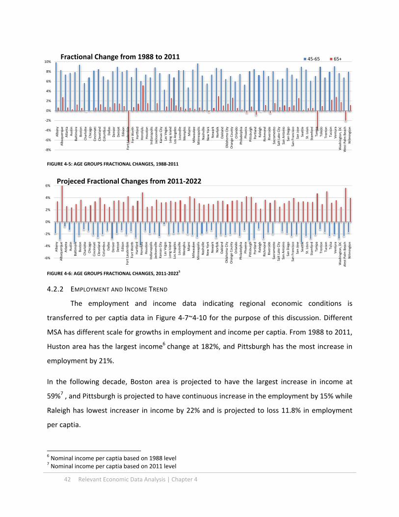
42 Relevant Economic Data Analysis | Chapter 4
FIGURE 4‐5: AGE GROUPS FRACTIONAL CHANGES, 1988‐2011
FIGURE 4‐6: AGE GROUPS FRACTIONAL CHANGES, 2011‐2022
5
4.2.2 EMPLOYMENT AND INCOME TREND
The employment and income data indicating regional economic conditions is
transferred to per captia data in Figure 4‐7~4‐10 for the purpose of this discussion. Different
MSA has different scale for growths in employment and income per captia. From 1988 to 2011,
Huston area has the largest income6 change at 182%, and Pittsburgh has the most increase in
employment by 21%.
In the following decade, Boston area is projected to have the largest increase in income at
59%7 , and Pittsburgh is projected to have continuous increase in the employment by 15% while
Raleigh has lowest increaser in income by 22% and is projected to loss 11.8% in employment
per captia.
6 Nominal income per captia based on 1988 level 7 Nominal income per captia based on 2011 level
‐8%
‐6%
‐4%
‐2%
0%
2%
4%
6%
8%
10%Albany
Albuquerque
Atlanta
Austin
Baltimore
Boston
Charlotte
Chicago
Cincinnati
Cleveland
Columbus
Dallas
Denver
Detroit
Edison
Fort Lauderdale
Fort W
orth
Hartford
Honolulu
Houston
Indianapolis
Jacksonville
Kansas City
Las Vegas
Long Island
Los Angeles
Louisville
Memphis
Miami
Milw
aukee
Minneapolis
Nashville
New York
Newark
Norfolk
Oakland
Oklahoma City
Orange County
Orlando
Philadelphia
Phoen
ix
Pittsburgh
Portland
Raleigh
Richmond
Riverside
Sacram
ento
Salt Lake City
San Antonio
San Diego
San Francisco
San Jose
Seattle
St. Louis
Stam
ford
Tampa
Toledo
Trenton
Tucson
Ven
tura
Washington, D
C
West Palm Beach
Wilm
ington
Fractional Change from 1988 to 2011 45‐65 65+
‐6%
‐4%
‐2%
0%
2%
4%
6%
Albany
Albuquerque
Atlanta
Austin
Baltimore
Boston
Charlotte
Chicago
Cincinnati
Cleveland
Columbus
Dallas
Denver
Detroit
Edison
Fort Lauderdale
Fort W
orth
Hartford
Honolulu
Houston
Indianapolis
Jacksonville
Kansas City
Las Vegas
Long Island
Los Angeles
Louisville
Memphis
Miami
Milw
aukee
Minneapolis
Nashville
New York
Newark
Norfolk
Oakland
Oklahoma City
Orange County
Orlando
Philadelphia
Phoen
ix
Pittsburgh
Portland
Raleigh
Richmond
Riverside
Sacram
ento
Salt Lake City
San Antonio
San Diego
San Francisco
San Jose
Seattle
St. Louis
Stam
ford
Tampa
Trenton
Tucson
Tulsa
Ven
tura
Washington, D
C
West Palm Beach
Wilm
ington
Projeced Fractional Changes from 2011‐2022

Chapter 4 | Relevant Economic Data Analysis 43
FIGURE 4‐7: PERCENTAGE CHANGE IN EMPLOYMENT PER CAPTIA, 1988‐2011
FIGURE 4‐8:PERCENTAGE CHANGE IN EMPLOYMENT PER CAPITA, 2011‐2022
FIGURE 4‐9: PERCENTAGE CHANGE IN INCOME PER CAPTIA, 1988‐2011
FIGURE 4‐10:PERCENTAGE CHANGE IN INCOME PER CAPTIA, 2011‐20225
‐20%
‐15%
‐10%
‐5%
0%
5%
10%
15%
20%
25%
Albany
Albuquerque
Atlanta
Austin
Baltimore
Boston
Charlotte
Chicago
Cincinnati
Cleveland
Columbus
Dallas
Denver
Detroit
Edison
Fort Lauderdale
Fort W
orth
Hartford
Honolulu
Houston
Indianapolis
Jacksonville
Kansas City
Las Vegas
Long Island
Los Angeles
Louisville
Memphis
Miami
Milw
aukee
Minneapolis
Nashville
New York
Newark
Norfolk
Oakland
Oklahoma City
Orange County
Orlando
Philadelphia
Phoen
ix
Pittsburgh
Portland
Raleigh
Richmond
Riverside
Sacram
ento
Salt Lake City
San Antonio
San Diego
San Francisco
San Jose
Seattle
St. Louis
Stam
ford
Tampa
Trenton
Tucson
Tulsa
Ven
tura
Washington, D
C
West Palm Beach
Wilm
ington
Percentage Change in Employment per captia 1988‐2011 Employment per captia
‐15%
‐10%
‐5%
0%
5%
10%
15%
20%
Albany
Albuquerque
Atlanta
Austin
Baltimore
Boston
Charlotte
Chicago
Cincinnati
Cleveland
Columbus
Dallas
Denver
Detroit
Edison
Fort Lauderdale
Fort W
orth
Hartford
Honolulu
Houston
Indianapolis
Jacksonville
Kansas City
Las Vegas
Long Island
Los Angeles
Louisville
Memphis
Miami
Milw
aukee
Minneapolis
Nashville
New York
Newark
Norfolk
Oakland
Oklahoma City
Orange County
Orlando
Philadelphia
Phoen
ix
Pittsburgh
Portland
Raleigh
Richmond
Riverside
Sacram
ento
Salt Lake City
San Antonio
San Diego
San Francisco
San Jose
Seattle
St. Louis
Stam
ford
Tampa
Trenton
Tucson
Tulsa
Ven
tura
Washington, D
C
West Palm Beach
Wilm
ington
Projected Percentage change in Employment per Captia 2011‐2022
50%
100%
150%
200%
Albany
Albuquerque
Atlanta
Austin
Baltimore
Boston
Charlotte
Chicago
Cincinnati
Cleveland
Columbus
Dallas
Denver
Detroit
Edison
Fort Lauderdale
Fort W
orth
Hartford
Honolulu
Houston
Indianapolis
Jacksonville
Kansas City
Las Vegas
Long Island
Los Angeles
Louisville
Memphis
Miami
Milw
aukee
Minneapolis
Nashville
New York
Newark
Norfolk
Oakland
Oklahoma City
Orange County
Orlando
Philadelphia
Phoen
ix
Pittsburgh
Portland
Raleigh
Richmond
Riverside
Sacram
ento
Salt Lake City
San Antonio
San Diego
San Francisco
San Jose
Seattle
St. Louis
Stam
ford
Tampa
Trenton
Tucson
Tulsa
Ven
tura
Washington, D
C
West Palm Beach
Wilm
ington
Percentage Change in Income per captia 1988‐ 2011 Income per captia
30%
80%
Albany
Albuquerque
Atlanta
Austin
Baltimore
Boston
Charlotte
Chicago
Cincinnati
Cleveland
Columbus
Dallas
Denver
Detroit
Edison
Fort Lauderdale
Fort W
orth
Hartford
Honolulu
Houston
Indianapolis
Jacksonville
Kansas City
Las Vegas
Long Island
Los Angeles
Louisville
Memphis
Miami
Milw
aukee
Minneapolis
Nashville
New York
Newark
Norfolk
Oakland
Oklahoma City
Orange County
Orlando
Philadelphia
Phoen
ix
Pittsburgh
Portland
Raleigh
Richmond
Riverside
Sacram
ento
Salt Lake City
San Antonio
San Diego
San Francisco
San Jose
Seattle
St. Louis
Stam
ford
Tampa
Trenton
Tucson
Tulsa
Ven
tura
Washington, D
C
West Palm Beach
Wilm
ington
Projected Percentage Change in Income per captia 2011‐2022

44 Relevant Economic Data Analysis | Chapter 4
4.3 HEALTH CARE EMPLOYMENT AND MOB
Comparing the historical health care employment with MOB stock, we can have a
glimpse of how the health care industry deploys the MOB for providing outpatient services.
Each section of health care services has different requirements of usages of MOB space and
these requirements dictate the scale of demand for the MOB market. In order to predict what
will happen to the MOB market in the future, we need to analyze how these sections grow and
shift in order to understand what drives the demand.
The market of medical services has increased in the past, the evidence lies in the fact
the growth of health care employment out‐paced total population and employment as
illustrated in Figure 4‐1. MOB grew at the similar pace as heath care employment. In the span
of 23 years, total employment grew by 23% and total population grew by 32%. Health care
employment in total, however, grew by 78%. Many factors to which medical practices
responded in recent history involve changes in health insurance practices, public health policies,
medical technology innovations, life style trends and consumer behaviors. We look into how
health care industry changes in responding to the changing market by examining changes in
sectors of health care employment data.
4.3.1 HEALTH CARE PRACTICE TRENDS IN TOTAL
Even though the overall health care industry is growing, not all sectors in health care
employment behave identically. In fact, the general trend for the share of hospital employment
25.2%
9.5%7.4%
7.0%3.1%
48.0%
Health Care Employment in 2011 Off_Phy
Off_Dent
Off_Others
Outpat
Labs
Hosp
21.7%
9.3%
4.7%
5.4%2.8%
56.2%
Health Care Employment in 1988
FIGURE 4‐11: HEALTH CARE EMPLOYMENT COMPOSITION

Chapter 4 | Relevant Economic Data Analysis 45
within health care industry has declined from 56% to 48% as shown in Figure 4‐11. Office of
dentists has slightest increase, and outpatient care center and medical and diagnostic
laboratories all have increases in shares. Shares of office of physicians, office of others,
outpatient centers and medical diagnostic and laboratories have all increased8.
The decreasing share of hospital
employment and increasing shares in others
demonstrate the shift of medical practice
from inpatient care to outpatient services as
discussed in the earlier chapter. The rates
each sectors grow and diminish at are
different though out the time. Figure 4‐12
shows different growth patterns in each
sector. This growth index is based on the
historical health care employment data that
has reflected all factors. Hospitals have been
steadily decreasing in percentage while office
of others had rapid growth in early 90s’ and
the growing trend dipped in late 90s’. Similar to office of others but more subtly, outpatient
center’s growth slowed in late 90s but fastened afterward9. The office of dentists and medical
diagnostic and laboratories had small fluctuations in growths in the past but medical diagnostic
and laboratories was increasing slightly recently. Office of physicians grew steadily and had a
slightly faster growth in late 90s’.
4.3.2 HEALTH CARE PRACTICE TRENDS IN EACH MSA
In terms of health care employment sector changes in individual MSA, the Figure 4‐13
demonstrates that most of the MSAs have lost shares in hospital employment and the
noticeable growth in the employment in other sectors. The largest growths in office of
physician and office of dentists occurred in Norfolk. Honolulu, Sacramento and Trenton have
8 Excluding social assistant because of its unclear usage of MOB 9 See Appendix E
60%
80%
100%
120%
140%
160%
180% Growth Index
Off_phy Off_Dent Off_Others
Outpat Labs Hosp
FIGURE 4‐12: SECTIONAL HEALTH CARE GROWTH INDEX

46 Relevant Economic Data Analysis | Chapter 4
the biggest changes in office of others, outpatient centers and medical diagnostic and
laboratories sectors respectively.
22% loss in hospital employment share happened in the area with the biggest fractional
gain in physicians and dentists, Norfolk. Some MSAs, opposite to the most, have increased
shares in hospital employment, and the largest increase of 6% happened in Seattle.
The most stable health care employment composition is in Boston area from 1988 to
2011, and the most volatile one is the Norfolk market10.
FIGURE 4‐13: FRACTIONAL CHANGES IN HEALTH CARE EMPLOYMENT SECTIOS, 1988‐2011
10 See Appendix F
‐20%
‐15%
‐10%
‐5%
0%
5%
10%
15%
20%Fractional Changes in Health Care Employment Sectors from 1988‐2011
‐20%
‐15%
‐10%
‐5%
0%
5%
10%
15%
20%
‐20%
‐15%
‐10%
‐5%
0%
5%
10%
15%
20%
Off_Phy Off_dent Off_Others Outpat Labs Hosp
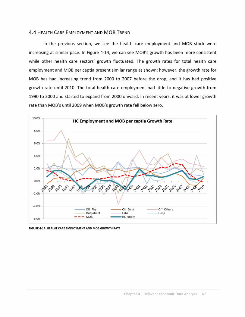
Chapter 4 | Relevant Economic Data Analysis 47
4.4 HEALTH CARE EMPLOYMENT AND MOB TREND
In the previous section, we see the health care employment and MOB stock were
increasing at similar pace. In Figure 4‐14, we can see MOB’s growth has been more consistent
while other health care sectors’ growth fluctuated. The growth rates for total health care
employment and MOB per captia present similar range as shown; however, the growth rate for
MOB has had increasing trend from 2000 to 2007 before the drop, and it has had positive
growth rate until 2010. The total health care employment had little to negative growth from
1990 to 2000 and started to expand from 2000 onward. In recent years, it was at lower growth
rate than MOB’s until 2009 when MOB’s growth rate fell below zero.
FIGURE 4‐14: HEALHT CARE EMPLOYMENT AND MOB GROWTH RATE
‐6.0%
‐4.0%
‐2.0%
0.0%
2.0%
4.0%
6.0%
8.0%
10.0%HC Employment and MOB per captia Growth Rate
Off_Phy Off_Dent Off_OthersOutpatient Labs HospMOB HC emply

48 Relevant Economic Data Analysis | Chapter 4
4.5 CHAPTER SUMMARY
Across 63 MSA, the population will continue to grow, although it will grow at the slower
rate in the next decade. The income will increase and the employment will grow along with
the total population. The health care employment had out‐grow the employment and the
population in the past.
The population age group 45+ is becoming larger share of total US population. The group
age 45‐65 grew larger in the population share and will entering the group age 65+,
increasing the share of the population group age 65+. Although growth patterns of group
age 45‐65, and group age 65+ in most of MSAs agree with the total aging trend, each MSA
has different rate of growths in 45‐65 and 65+, depending on how each MSA grow in
population.
Different MSA has the different outlook for employment and income, such outlook is not
related to the demographic trend. Regional economic matrices will be separate sets of
factors for the MOB growth.
Within the growing health care employment, the shift among sectors illustrates the
changing practice in medical services. The rapid growing sectors such as office of the others,
outpatient care centers and office of physicians represent the trend of increasing outpatient
services.
Regional factors again affect how health care practices change. Some MSA have minor shifts
in the health care employment composition and some have major changes in the medical
practices from 1988 to 2011.
MOB grew along with the overall health care employment, but with different growth
patterns.

Chapter 5 | Medical Office Building Model 49
Chapter 5. MEDICAL OFFICE BUILDING MODEL
5.1 DEFINITION
The purpose of this chapter is to study the how much individual factors influence MOB
in order to set up forecasts for the MOB for individual markets. Using panel regression to
capture the relationships among regional and temporal effects in addition to the assumed
demand and supply factors, we present the results from regressions and construct the system
to explain MOB market in this chapter.
5.2 TOP‐TIER: MOB MODEL
We established that MOB stock changes depend on the following categories: Offices of
Physicians, Office of Dentists, Outpatient Care Centers, Medical and Diagnostic Laboratories,
and General and Surgical Hospitals because generally these are establishments using MOB
spaces. Using the fixed‐effect regression to create dummy variables for each MSA and each
year, we build the model from panel regression result (Table 5‐1) takes form as Equation 5‐1. In
the model, k and g correspond with MSA number and year number respectively1.
MOB = 1,313,392 + IMSA_K + IYEAR_G +120,880 X OFF_PHY + 414,729 X OFF_DENT – 156,728 X
OFF_OTHERS ‐86,499 X OUTPAT + 307,486 X LABS + 67,467 X HOSP
(5‐1)
MOB R2 0.98
_IMSA_1‐62 N 1,488
_Iyear_1988‐2011 * p<0.05
** p<0.01
Off_Phy 120,880 _IMSA_20 7,446,773 _IMSA_44 ‐92,927 _Iyear_1989 100,315
(5.96)** (14.00)** ‐0.63 ‐0.59
Off_Dent 414,729 _IMSA_21 998,298 _IMSA_45 ‐1,816,366 _Iyear_1990 169,235
(6.74)** (4.49)** (19.60)** ‐1
Off_Others ‐156,728 _IMSA_22 ‐1,497,304 _IMSA_46 970,390 _Iyear_1991 179,770
(3.92)** (9.11)** (3.99)** ‐1.09
Outpat ‐86,499 _IMSA_23 ‐1,097,099 _IMSA_47 ‐421,006 _Iyear_1992 186,867
1 See Table 2‐3 for the full list of MSA

50 Medical Office Building Model | Chapter 5
(3.56)** (5.22)** (2.10)* ‐1.15
Labs 307,486 _IMSA_24 2,987,630 _IMSA_48 ‐266,312 _Iyear_1993 177,951
(4.59)** (9.54)** ‐1.54 ‐1.1
Hosp 67,467 _IMSA_25 ‐2,506,095 _IMSA_49 2,116,079 _Iyear_1994 253,423
(4.76)** (5.71)** (14.80)** ‐1.62
_IMSA_2 952,439 _IMSA_26 9,170,975 _IMSA_50 3,205,674 _Iyear_1995 276,852
(5.30)** (7.45)** (13.34)** ‐1.81
_IMSA_3 3,667,331 _IMSA_27 1,084,162 _IMSA_51 ‐1,178,422 _Iyear_1996 282,111
(7.34)** (9.74)** (5.16)** ‐1.87
_IMSA_4 ‐1,002,434 _IMSA_28 1,489,732 _IMSA_52 ‐226,807 _Iyear_1997 303,101
(10.14)** (11.58)** ‐0.83 (2.02)*
_IMSA_5 ‐4,890,677 _IMSA_29 595,377 _IMSA_53 5,945,730 _Iyear_1998 312,519
(10.19)** (2.19)* (11.97)** (2.08)*
_IMSA_6 ‐5,028,434 _IMSA_30 ‐361,581 _IMSA_54 ‐2,186,544 _Iyear_1999 247,201
(3.97)** ‐1.71 (4.61)** ‐1.64
_IMSA_7 1,618,899 _IMSA_31 2,892,374 _IMSA_55 ‐949,174 _Iyear_2000 296,592
(6.10)** (7.74)** (6.45)** ‐1.95
_IMSA_8 ‐4,784,250 _IMSA_32 ‐573,813 _IMSA_56 ‐958,729 _Iyear_2001 298,175
(3.08)** (3.34)** (2.95)** ‐1.9
_IMSA_9 ‐1,236,329 _IMSA_33 ‐15,086,721 _IMSA_57 ‐635,559 _Iyear_2002 287,542
(4.76)** (6.59)** (6.69)** ‐1.78
_IMSA_10 ‐116,483 _IMSA_34 ‐2,693,676 _IMSA_58 462,311 _Iyear_2003 355,225
‐0.26 (8.87)** (5.96)** (2.17)*
_IMSA_11 2,316,078 _IMSA_35 ‐365,149 _IMSA_59 ‐1,009,673 _Iyear_2004 473,335
(11.11)** ‐1.54 (5.83)** (2.73)**
_IMSA_12 2,502,848 _IMSA_36 524,691 _IMSA_60 ‐3,611,993 _Iyear_2005 678,054
(7.01)** ‐1.78 (6.31)** (3.66)**
_IMSA_13 1,850,868 _IMSA_37 976,107 _IMSA_61 1,453,177 _Iyear_2006 869,711
(5.79)** (8.74)** (11.62)** (4.37)**
_IMSA_14 11,113,491 _IMSA_38 3,149,089 _IMSA_62 ‐1,909,516 _Iyear_2007 1,080,818
(12.24)** (9.70)** (15.54)** (5.10)**
_IMSA_15 ‐1,590,801 _IMSA_39 ‐1,082,811 _Iyear_2008 1,298,250
(5.99)** (6.26)** (5.76)**
_IMSA_16 746,153 _IMSA_40 ‐3,870,112 _Iyear_2009 1,465,975
(3.64)** (3.64)** (6.34)**
_IMSA_17 9,370,418 _IMSA_41 4,073,034 _Iyear_2010 1,527,107
(21.99)** (11.10)** (6.52)**
_IMSA_18 ‐643,031 _IMSA_42 ‐1,780,067 _Iyear_2011 1,525,325
(5.05)** (3.71)** (6.40)**
_IMSA_19 ‐1,566,731 _IMSA_43 ‐184,506 _cons 1,313,392
(15.50)** ‐0.9 (6.34)**
TABLE 5‐1: MOB REGRESSION RESULT

Chapter 5 | Medical Office Building Model 51
This model explains how each business demands different amount of MOB spaces with
regard health care sectors. The coefficients presented in the Equation are ratios of how many
square footage used by a thousand of health care employment. For offices of dentists, every
employee uses up to 414.7 square feet for MOB space. This could explain the fact that each
dentist tends to have its own office as the sole practitioner for the business; and for medical
and diagnostic laboratories, every employee occupied 307.5 square feet, including the share of
equipment and supplement space required for laboratories. For every office of physician and
hospital employee, 120.8 and 67.5 square feet of space are generated each for their usage
demands. This might be because physicians and group practices co‐operating these business
establishments and share the spaces with rotating schedule; for hospitals, MOB only
represents a portion of its operating facilities, and this ratio represents partial of its space usage
per employee. Never the less, hospitals have significant demand on MOB space for their large
number of employment.
Negative signs of coefficients presented in the model suggest that certain type of
establishments decrease MOB stocks. The trend in development larger outpatient care center
introducing more efficient use of health care work force and consolidating MOB spaces
resulting every one employee in outpatient care center decreases 86.5 square feet of spaces;
Office of others have more flexibility to setup establishments in more retail/commercial
oriented spaces rather than medical type of
premises, resulting every one employee
decreases 156.7 square feet of MOB spaces.
Although hospitals and physicians has
less impact in MOB per employee in terms of
space usage, the larger number of employee
still signify the large demand for MOB. In
referencing to Figure 4‐11, Hospitals comprise
around 48% and office of physician represent
25% of all health care employment in 2011,
Weighted Influences for MOB
Off_Phy
Off_Dent
Off_Other
Outpat
Labs
Hosp
FIGURE 5‐1:WEIGHTED INFLUENCES FOR MOB

52 Medical Office Building Model | Chapter 5
even with less values of coefficients, hospital and offices of physicians still have significant
impact on MOB. Figure 5‐1 demonstrates health care sectors’ influences that combine absolute
values of coefficients and share of health care employment. Offices of dentists, offices of
physicians and hospitals all have great impacts on MOB spaces, and medical and diagnostic
laboratories with smaller numbers of employment have less demand on MOB space as the
result.
Note that the coefficients for MSA variables range from 11,113,491 (Detroit) to ‐
15,086,721 (New York), demonstrating differences in regions. Local characteristics such as
history in medical development, availability for additional development, political environment,
and geographical condition could all contribute to these differences.
The values of coefficient of time
variable were increasing rapidly from 2002
to 2008 compare to previous decade as
Figure 5‐1 shown. The time variable presents
the trend note dictated by the locality or the
health care employment condition, and
could represent the influences from other
factors such as investment preferences or
policy incentives occurred over the time. We
will use the trend extracted from time
variable to replicate future trend to forecast
MOB in the next chapter.
0
200,000
400,000
600,000
800,000
1,000,000
1,200,000
1,400,000
1,600,000
1,800,000
MOB Time Variable
Coefficient
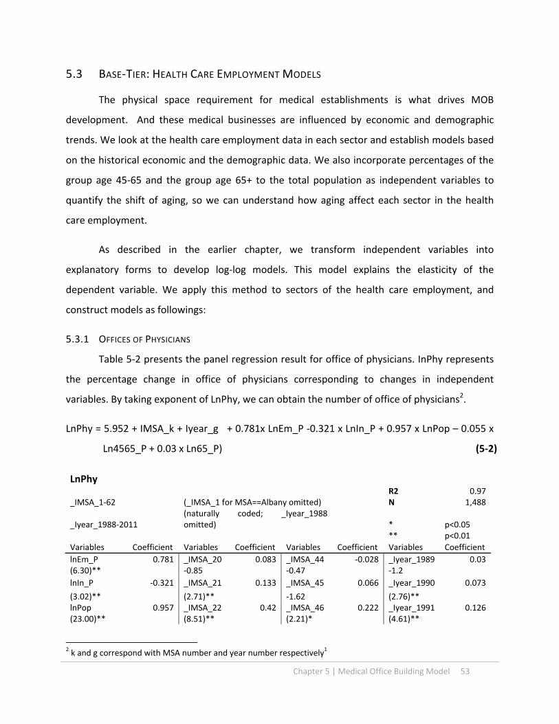
Chapter 5 | Medical Office Building Model 53
5.3 BASE‐TIER: HEALTH CARE EMPLOYMENT MODELS
The physical space requirement for medical establishments is what drives MOB
development. And these medical businesses are influenced by economic and demographic
trends. We look at the health care employment data in each sector and establish models based
on the historical economic and the demographic data. We also incorporate percentages of the
group age 45‐65 and the group age 65+ to the total population as independent variables to
quantify the shift of aging, so we can understand how aging affect each sector in the health
care employment.
As described in the earlier chapter, we transform independent variables into
explanatory forms to develop log‐log models. This model explains the elasticity of the
dependent variable. We apply this method to sectors of the health care employment, and
construct models as followings:
5.3.1 OFFICES OF PHYSICIANS
Table 5‐2 presents the panel regression result for office of physicians. InPhy represents
the percentage change in office of physicians corresponding to changes in independent
variables. By taking exponent of LnPhy, we can obtain the number of office of physicians2.
LnPhy = 5.952 + IMSA_k + Iyear_g + 0.781x LnEm_P ‐0.321 x LnIn_P + 0.957 x LnPop – 0.055 x
Ln4565_P + 0.03 x Ln65_P) (5‐2)
LnPhy R2 0.97
_IMSA_1‐62 (_IMSA_1 for MSA==Albany omitted) N 1,488
_Iyear_1988‐2011 (naturally coded; _Iyear_1988 omitted) * p<0.05
** p<0.01
Variables Coefficient Variables Coefficient Variables Coefficient Variables Coefficient
lnEm_P 0.781 _IMSA_20 0.083 _IMSA_44 ‐0.028 _Iyear_1989 0.03(6.30)** ‐0.85 ‐0.47 ‐1.2
lnIn_P ‐0.321 _IMSA_21 0.133 _IMSA_45 0.066 _Iyear_1990 0.073
(3.02)** (2.71)** ‐1.62 (2.76)** lnPop 0.957 _IMSA_22 0.42 _IMSA_46 0.222 _Iyear_1991 0.126(23.00)** (8.51)** (2.21)* (4.61)**
2 k and g correspond with MSA number and year number respectively1
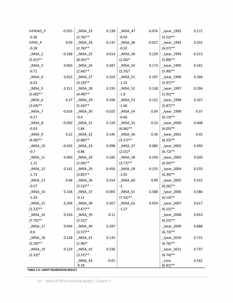
54 Medical Office Building Model | Chapter 5
lnP4565_P ‐0.055 _IMSA_23 0.138 _IMSA_47 0.076 _Iyear_1992 0.171
‐0.36 (2.76)** ‐0.93 (5.52)**
lnP65_P 0.03 _IMSA_24 ‐0.137 _IMSA_48 ‐0.027 _Iyear_1993 0.201
‐0.28 (2.76)** ‐0.32 (6.07)**
_IMSA_2 ‐0.268 _IMSA_25 0.614 _IMSA_49 0.129 _Iyear_1994 0.213
(5.41)** (8.26)** (2.06)* (5.88)**
_IMSA_3 0.063 _IMSA_26 0.287 _IMSA_50 0.173 _Iyear_1995 0.241
‐0.71 (2.66)** (2.35)* (5.99)**
_IMSA_4 0.022 _IMSA_27 0.163 _IMSA_51 0.107 _Iyear_1996 0.266
‐0.25 (4.19)** ‐1.31 (5.97)**
_IMSA_5 0.311 _IMSA_28 0.235 _IMSA_52 0.138 _Iyear_1997 0.294
(5.00)** (4.49)** ‐1.8 (5.95)**
_IMSA_6 0.27 _IMSA_29 0.296 _IMSA_53 0.121 _Iyear_1998 0.327
(3.04)** (5.43)** ‐1.66 (5.87)**
_IMSA_7 ‐0.014 _IMSA_30 ‐0.025 _IMSA_54 0.04 _Iyear_1999 0.37
‐0.27 ‐0.4 ‐0.66 (6.13)**
_IMSA_8 ‐0.002 _IMSA_31 0.129 _IMSA_55 0.52 _Iyear_2000 0.408
‐0.02 ‐1.84 (6.86)** (6.05)**
_IMSA_9 0.21 _IMSA_32 0.145 _IMSA_56 0.36 _Iyear_2001 0.45
(4.00)** (2.88)** (5.27)** (6.35)**
_IMSA_10 ‐0.042 _IMSA_33 0.098 _IMSA_57 0.085 _Iyear_2002 0.495
‐0.7 ‐0.86 (2.01)* (6.72)**
_IMSA_11 0.063 _IMSA_34 0.185 _IMSA_58 0.193 _Iyear_2003 0.505
‐1.15 (2.94)** (3.77)** (6.50)**
_IMSA_12 0.161 _IMSA_35 ‐0.456 _IMSA_59 0.155 _Iyear_2004 0.533
‐1.73 (3.85)** ‐1.92 (6.39)**
_IMSA_13 0.04 _IMSA_36 0.314 _IMSA_60 0.09 _Iyear_2005 0.555
‐0.57 (3.52)** ‐1 (6.26)**
_IMSA_14 0.104 _IMSA_37 ‐0.005 _IMSA_61 0.588 _Iyear_2006 0.586
‐1.29 ‐0.11 (7.42)** (6.14)**
_IMSA_15 0.204 _IMSA_38 0.267 _IMSA_62 0.054 _Iyear_2007 0.617
(3.22)** (3.47)** ‐1.27 (6.15)**
_IMSA_16 0.416 _IMSA_39 0.11 _Iyear_2008 0.653
(7.70)** (2.31)* (6.25)**
_IMSA_17 0.044 _IMSA_40 0.297 _Iyear_2009 0.688
‐0.6 (3.57)** (6.73)**
_IMSA_18 0.228 _IMSA_41 0.133 _Iyear_2010 0.715
(5.29)** (1.96)* (6.76)**
_IMSA_19 0.124 _IMSA_42 0.236 _Iyear_2011 0.737
(2.32)* (3.37)** (6.74)**
_IMSA_43 ‐0.01 _cons ‐3.541 ‐0.18 (6.81)**
TABLE 5‐2: LNPHY REGRESSION RESULT
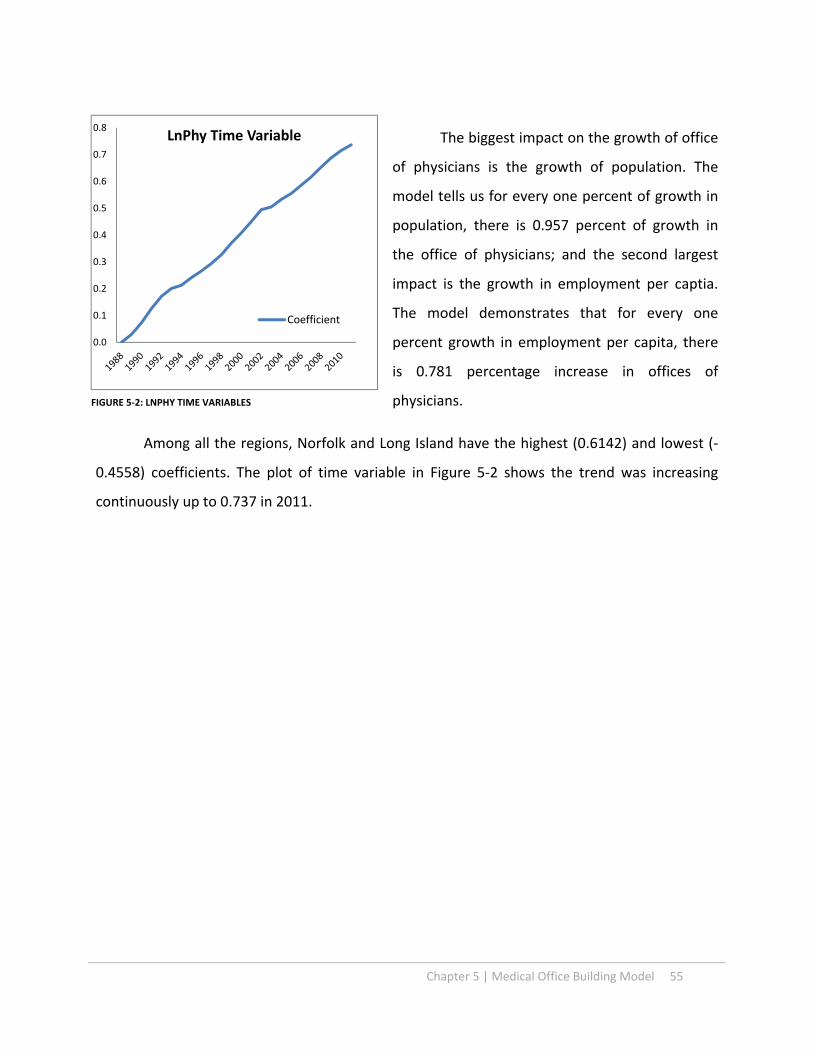
Chapter 5 | Medical Office Building Model 55
The biggest impact on the growth of office
of physicians is the growth of population. The
model tells us for every one percent of growth in
population, there is 0.957 percent of growth in
the office of physicians; and the second largest
impact is the growth in employment per captia.
The model demonstrates that for every one
percent growth in employment per capita, there
is 0.781 percentage increase in offices of
physicians.
Among all the regions, Norfolk and Long Island have the highest (0.6142) and lowest (‐
0.4558) coefficients. The plot of time variable in Figure 5‐2 shows the trend was increasing
continuously up to 0.737 in 2011.
0.0
0.1
0.2
0.3
0.4
0.5
0.6
0.7
0.8LnPhy Time Variable
Coefficient
FIGURE 5‐2: LNPHY TIME VARIABLES

56 Medical Office Building Model | Chapter 5
5.3.2 OFFICES OF DENTISTS
The following table and equation present the panel regression result for office of
physicians. LnDent represents the percentage change in office of dentists corresponding to
changes in independent variables. By taking exponent of LnDent, we can produce the number
of office of dentists2.
LnDent = ‐3.228 + IMSA_k + Iyear_g + 0.371x LnEm_P +0.022 x LnIn_P + 1.18 x LnPop +0.076 x
Ln4565_P + 0.532 x Ln65_P) (5‐3)
LnDent
R2 0.99
_IMSA_1‐62 (_IMSA_1 for MSA==Albany omitted) N 1,488
_Iyear_1988‐2011 (naturally coded; _Iyear_1988 omitted) * p<0.05
** p<0.01
Variables Coefficient Variables Coefficient Variables Coefficient Variables Coefficient
lnEm_P 0.371 _IMSA_20 ‐0.149 _IMSA_44 0.187 _Iyear_1989 ‐0.017
(4.47)** (2.27)* (4.97)** ‐1.01
lnIn_P 0.022 _IMSA_21 ‐0.013 _IMSA_45 0.018 _Iyear_1990 ‐0.022
‐0.28 ‐0.44 ‐0.97 ‐1.17
lnPop 1.18 _IMSA_22 ‐0.009 _IMSA_46 ‐0.094 _Iyear_1991 ‐0.01
(41.07)** ‐0.29 ‐1.21 ‐0.5
lnP4565_P 0.076 _IMSA_23 ‐0.049 _IMSA_47 0.334 _Iyear_1992 ‐0.006
‐0.67 ‐1.8 (8.94)** ‐0.25
lnP65_P 0.532 _IMSA_24 ‐0.12 _IMSA_48 0.491 _Iyear_1993 0.004
(7.24)** (3.47)** (8.30)** ‐0.15
_IMSA_2 0.25 _IMSA_25 0.158 _IMSA_49 ‐0.174 _Iyear_1994 0.011
(8.07)** (3.81)** (4.01)** ‐0.42
_IMSA_3 ‐0.048 _IMSA_26 ‐0.151 _IMSA_50 0.028 _Iyear_1995 0.028
‐0.82 (2.08)* ‐0.6 ‐0.96
_IMSA_4 0.148 _IMSA_27 ‐0.127 _IMSA_51 0.313 _Iyear_1996 0.035
(2.35)* (7.40)** (7.91)** ‐1.07
_IMSA_5 ‐0.097 _IMSA_28 ‐0.141 _IMSA_52 0.598 _Iyear_1997 0.047
(2.96)** (4.38)** (14.61)** ‐1.3
_IMSA_6 ‐0.063 _IMSA_29 ‐0.201 _IMSA_53 0.299 _Iyear_1998 0.054
‐1.22 (5.90)** (7.49)** ‐1.32
_IMSA_7 ‐0.047 _IMSA_30 0.075 _IMSA_54 ‐0.226 _Iyear_1999 0.072
‐1.41 (3.48)** (6.52)** ‐1.64
_IMSA_8 ‐0.22 _IMSA_31 0.05 _IMSA_55 0.314 _Iyear_2000 0.082
(3.46)** ‐1.16 (6.13)** ‐1.66
_IMSA_9 ‐0.083 _IMSA_32 ‐0.072 _IMSA_56 ‐0.246 _Iyear_2001 0.102
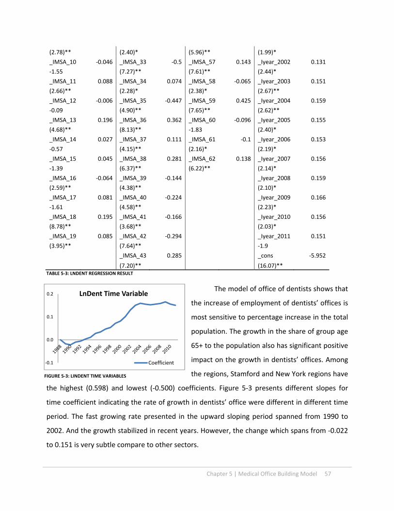
Chapter 5 | Medical Office Building Model 57
(2.78)** (2.40)* (5.96)** (1.99)*
_IMSA_10 ‐0.046 _IMSA_33 ‐0.5 _IMSA_57 0.143 _Iyear_2002 0.131
‐1.55 (7.27)** (7.61)** (2.44)*
_IMSA_11 0.088 _IMSA_34 0.074 _IMSA_58 ‐0.065 _Iyear_2003 0.151
(2.66)** (2.28)* (2.38)* (2.67)**
_IMSA_12 ‐0.006 _IMSA_35 ‐0.447 _IMSA_59 0.425 _Iyear_2004 0.159
‐0.09 (4.90)** (7.65)** (2.62)**
_IMSA_13 0.196 _IMSA_36 0.362 _IMSA_60 ‐0.096 _Iyear_2005 0.155
(4.68)** (8.13)** ‐1.83 (2.40)*
_IMSA_14 0.027 _IMSA_37 0.111 _IMSA_61 ‐0.1 _Iyear_2006 0.153
‐0.57 (4.15)** (2.16)* (2.19)*
_IMSA_15 0.045 _IMSA_38 0.281 _IMSA_62 0.138 _Iyear_2007 0.156
‐1.39 (6.37)** (6.22)** (2.14)*
_IMSA_16 ‐0.064 _IMSA_39 ‐0.144 _Iyear_2008 0.159
(2.59)** (4.38)** (2.10)*
_IMSA_17 0.081 _IMSA_40 ‐0.224 _Iyear_2009 0.166
‐1.61 (4.58)** (2.23)*
_IMSA_18 0.195 _IMSA_41 ‐0.166 _Iyear_2010 0.156
(8.78)** (3.68)** (2.03)*
_IMSA_19 0.085 _IMSA_42 ‐0.294 _Iyear_2011 0.151
(3.95)** (7.64)** ‐1.9
_IMSA_43 0.285 _cons ‐5.952
(7.20)** (16.07)** TABLE 5‐3: LNDENT REGRESSION RESULT
The model of office of dentists shows that
the increase of employment of dentists’ offices is
most sensitive to percentage increase in the total
population. The growth in the share of group age
65+ to the population also has significant positive
impact on the growth in dentists’ offices. Among
the regions, Stamford and New York regions have
the highest (0.598) and lowest (‐0.500) coefficients. Figure 5‐3 presents different slopes for
time coefficient indicating the rate of growth in dentists’ office were different in different time
period. The fast growing rate presented in the upward sloping period spanned from 1990 to
2002. And the growth stabilized in recent years. However, the change which spans from ‐0.022
to 0.151 is very subtle compare to other sectors.
‐0.1
0.0
0.1
0.2 LnDent Time Variable
Coefficient
FIGURE 5‐3: LINDENT TIME VARIABLES
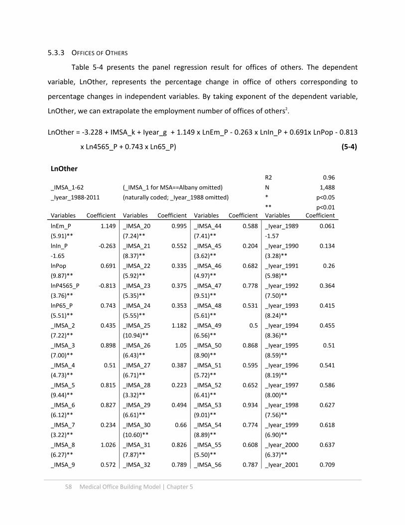
58 Medical Office Building Model | Chapter 5
5.3.3 OFFICES OF OTHERS
Table 5‐4 presents the panel regression result for offices of others. The dependent
variable, LnOther, represents the percentage change in office of others corresponding to
percentage changes in independent variables. By taking exponent of the dependent variable,
LnOther, we can extrapolate the employment number of offices of others2.
LnOther = ‐3.228 + IMSA_k + Iyear_g + 1.149 x LnEm_P ‐ 0.263 x LnIn_P + 0.691x LnPop ‐ 0.813
x Ln4565_P + 0.743 x Ln65_P) (5‐4)
LnOther R2 0.96
_IMSA_1‐62 (_IMSA_1 for MSA==Albany omitted) N 1,488
_Iyear_1988‐2011 (naturally coded; _Iyear_1988 omitted) * p<0.05
** p<0.01 Variables Coefficient Variables Coefficient Variables Coefficient Variables Coefficient
lnEm_P 1.149 _IMSA_20 0.995 _IMSA_44 0.588 _Iyear_1989 0.061
(5.91)** (7.24)** (7.41)** ‐1.57
lnIn_P ‐0.263 _IMSA_21 0.552 _IMSA_45 0.204 _Iyear_1990 0.134
‐1.65 (8.37)** (3.62)** (3.28)**
lnPop 0.691 _IMSA_22 0.335 _IMSA_46 0.682 _Iyear_1991 0.26
(9.87)** (5.92)** (4.97)** (5.98)**
lnP4565_P ‐0.813 _IMSA_23 0.375 _IMSA_47 0.778 _Iyear_1992 0.364
(3.76)** (5.35)** (9.51)** (7.50)**
lnP65_P 0.743 _IMSA_24 0.353 _IMSA_48 0.531 _Iyear_1993 0.415
(5.51)** (5.55)** (5.61)** (8.24)**
_IMSA_2 0.435 _IMSA_25 1.182 _IMSA_49 0.5 _Iyear_1994 0.455
(7.22)** (10.94)** (6.56)** (8.36)**
_IMSA_3 0.898 _IMSA_26 1.05 _IMSA_50 0.868 _Iyear_1995 0.51
(7.00)** (6.43)** (8.90)** (8.59)**
_IMSA_4 0.51 _IMSA_27 0.387 _IMSA_51 0.595 _Iyear_1996 0.541
(4.73)** (6.71)** (5.72)** (8.19)**
_IMSA_5 0.815 _IMSA_28 0.223 _IMSA_52 0.652 _Iyear_1997 0.586
(9.44)** (3.32)** (6.41)** (8.00)**
_IMSA_6 0.827 _IMSA_29 0.494 _IMSA_53 0.934 _Iyear_1998 0.627
(6.12)** (6.61)** (9.01)** (7.56)**
_IMSA_7 0.234 _IMSA_30 0.66 _IMSA_54 0.774 _Iyear_1999 0.618
(3.22)** (10.60)** (8.89)** (6.90)**
_IMSA_8 1.026 _IMSA_31 0.826 _IMSA_55 0.608 _Iyear_2000 0.637
(6.27)** (7.87)** (5.50)** (6.37)**
_IMSA_9 0.572 _IMSA_32 0.789 _IMSA_56 0.787 _Iyear_2001 0.709

Chapter 5 | Medical Office Building Model 59
(8.08)** (12.57)** (8.01)** (6.72)**
_IMSA_10 0.549 _IMSA_33 0.841 _IMSA_57 0.607 _Iyear_2002 0.813
(7.16)** (4.75)** (10.45)** (7.36)**
_IMSA_11 0.574 _IMSA_34 0.653 _IMSA_58 0.096 _Iyear_2003 0.877
(8.04)** (7.34)** ‐1.52 (7.55)**
_IMSA_12 0.985 _IMSA_35 0.031 _IMSA_59 0.873 _Iyear_2004 0.94
(7.84)** ‐0.27 (7.74)** (7.48)**
_IMSA_13 1.003 _IMSA_36 0.828 _IMSA_60 0.809 _Iyear_2005 0.996
(10.30)** (7.83)** (5.82)** (7.46)**
_IMSA_14 1.026 _IMSA_37 0.434 _IMSA_61 0.539 _Iyear_2006 1.043
(8.68)** (7.88)** (5.48)** (7.29)**
_IMSA_15 0.964 _IMSA_38 1.08 _IMSA_62 0.264 _Iyear_2007 1.09
(11.07)** (10.63)** (4.40)** (7.33)**
_IMSA_16 0.683 _IMSA_39 0.428 _Iyear_2008 1.154
(10.36)** (6.38)** (7.44)**
_IMSA_17 0.827 _IMSA_40 1.052 _Iyear_2009 1.234
(9.32)** (8.30)** (8.08)**
_IMSA_18 0.566 _IMSA_41 0.698 _Iyear_2010 1.279
(6.69)** (7.41)** (8.09)**
_IMSA_19 0.046 _IMSA_42 0.828 _Iyear_2011 1.307
‐0.62 (8.58)** (8.02)**
_IMSA_43 0.651 _cons ‐3.228
(6.72)** (4.29)** TABLE 5‐4: LNOTHERS REGRESSION RESULT
The office of others model shows that the increase of employment of others’ offices is
the most elastic to the employment per captia. The growth in share of group age 65+ in
population also has significant positive impact on the growth in others’ offices, but group 45‐65
percentage change has negative impact on the growth of office of others. Among MSAs, Long
Island and Norfolk regions have the highest
(1.182) and the lowest (0.031) coefficients.
The time variable coefficients in Figure 5‐
4 presents gentle upward slope, indicating that
the development trend of others’ offices was
fairly stable with little changes from 1988 to
2011.
0.0
0.1
0.2LnOthers Time Variable
Coefficient
FIGURE 5‐4: LNOTHERS TIME VARIABLES

60 Medical Office Building Model | Chapter 5
5.3.5 OUTPATIENT CARE CENTERS
The following table presents the panel regression result for outpatient care centers. By
taking exponent of dependent variable, lnOutpat, we can get the number of employee for
outpatient care centers.
LnOutpat = ‐5.994 + IMSA_k + Iyear_g + 0.129 x LnEm_P ‐0.449 x LnIn_P + 0.835 x LnPop ‐1.49
x Ln4565_P + 0.34 x Ln65_P (5‐5)
LnOutpat
(_IMSA_1 for MSA==Albany omitted) R2 0.93
(naturally coded; _Iyear_1988 omitted) N 1,488
* p<0.05
** p<0.01 Variables Coefficient Variables Coefficient Variables Coefficient Variables Coefficient
lnEm_P 0.129 _IMSA_20 ‐0.392 _IMSA_44 ‐0.543 _Iyear_1989 0.035
‐0.55 (1.96)* (4.45)** ‐0.65
lnIn_P ‐0.449 _IMSA_21 ‐0.098 _IMSA_45 ‐0.269 _Iyear_1990 0.092
(2.00)* ‐1.01 (3.29)** ‐1.64
lnPop 0.835 _IMSA_22 0.092 _IMSA_46 ‐0.663 _Iyear_1991 0.156
(9.71)** ‐1.04 (3.63)** (2.84)**
lnP4565_P ‐1.49 _IMSA_23 0.219 _IMSA_47 0.419 _Iyear_1992 0.269
(4.89)** (2.04)* (3.54)** (4.22)**
lnP65_P 0.34 _IMSA_24 ‐0.318 _IMSA_48 ‐0.811 _Iyear_1993 0.349
‐1.43 (3.45)** (5.27)** (5.12)**
_IMSA_2 0.784 _IMSA_25 0.375 _IMSA_49 ‐0.573 _Iyear_1994 0.433
(7.38)** (2.56)* (4.64)** (5.75)**
_IMSA_3 ‐0.382 _IMSA_26 0.378 _IMSA_50 0.191 _Iyear_1995 0.511
(2.13)* ‐1.76 ‐1.32 (6.05)**
_IMSA_4 ‐1.115 _IMSA_27 0.305 _IMSA_51 0.735 _Iyear_1996 0.59
(6.36)** (4.99)** (4.72)** (6.21)**
_IMSA_5 0.192 _IMSA_28 ‐0.026 _IMSA_52 0.092 _Iyear_1997 0.671
‐1.66 ‐0.25 ‐0.6 (6.37)**
_IMSA_6 0.872 _IMSA_29 0.29 _IMSA_53 1.05 _Iyear_1998 0.742
(5.00)** (2.94)** (7.37)** (6.20)**
_IMSA_7 ‐0.601 _IMSA_30 0.528 _IMSA_54 0.006 _Iyear_1999 0.78
(5.88)** (4.88)** ‐0.05 (6.01)**
_IMSA_8 ‐0.215 _IMSA_31 0.428 _IMSA_55 ‐0.471 _Iyear_2000 0.855
‐1.06 (3.00)** (3.02)** (5.84)**
_IMSA_9 0.061 _IMSA_32 0.435 _IMSA_56 0.359 _Iyear_2001 0.913
‐0.6 (4.80)** (2.69)** (5.88)**
_IMSA_10 0.393 _IMSA_33 0.47 _IMSA_57 0.314 _Iyear_2002 0.978

Chapter 5 | Medical Office Building Model 61
(4.00)** (2.06)* (4.32)** (6.05)**
_IMSA_11 ‐0.16 _IMSA_34 0.065 _IMSA_58 0.063 _Iyear_2003 1.033
‐1.6 ‐0.49 ‐0.7 (6.05)**
_IMSA_12 ‐0.362 _IMSA_35 0.616 _IMSA_59 ‐0.35 _Iyear_2004 1.113
‐1.91 (2.87)** (2.20)* (6.05)**
_IMSA_13 0.806 _IMSA_36 0.718 _IMSA_60 0.598 _Iyear_2005 1.206
(5.77)** (4.24)** (3.09)** (6.14)**
_IMSA_14 0.362 _IMSA_37 0.071 _IMSA_61 ‐0.225 _Iyear_2006 1.308
(2.35)* ‐0.91 ‐1.64 (6.21)**
_IMSA_15 ‐0.458 _IMSA_38 ‐0.171 _IMSA_62 ‐0.189 _Iyear_2007 1.379
(3.42)** ‐1.1 (2.42)* (6.27)**
_IMSA_16 ‐0.514 _IMSA_39 ‐0.442 _Iyear_2008 1.44
(5.23)** (4.67)** (6.31)**
_IMSA_17 ‐0.555 _IMSA_40 0.517 _Iyear_2009 1.451
(3.94)** (3.21)** (6.55)**
_IMSA_18 0.031 _IMSA_41 0.36 _Iyear_2010 1.486
‐0.41 (2.87)** (6.55)**
_IMSA_19 ‐0.483 _IMSA_42 0.17 _Iyear_2011 1.515
(4.32)** ‐1.37 (6.52)**
_IMSA_43 0.701 _cons ‐5.994
(6.89)** (5.33)** TABLE 5‐5: INOUTPAT REGRESSION RESULT
The model shows that the development of
outpatient care centers is fairly elastic to total
population. The group 45‐65 percentage change
has negative impact on the growth of outpatient
care centers. Among the regions, Seattle and
Austin regions have the highest (1.050) and
lowest (‐0.115) coefficients.
Figure 5‐5 populated with time variables
from the log model for outpatient care centers
shows the rapid increase in coefficient from 1988
to 2011. The range of the value of time
coefficients at 1.51 is the largest among health care employment models, and this implies
outpatient care center has the strongest growing trend among all health care sectors.
0.0
0.1
0.2
0.3
0.4
0.5
0.6
0.7
0.8
0.9
1.0
1.1
1.2
1.3
1.4
1.5
1.6LnOut Time Variables
Coefficient
FIGURE 5‐5: LNOUT TIME VARIABLES

62 Medical Office Building Model | Chapter 5
5.3.6 MEDICAL AND DIAGNOSTIC LABORATORIES
The following table and equation are from the panel regression result for medical and
diagnostic laboratories. By taking exponent of the dependent variable, LnLabs, we can construct
the employment number of medical and diagnostic laboratories for specific area and year.
LnLabs = ‐0.8938 + IMSA_k + Iyear_g + 1.207 x LnEm_P ‐0.832 x LnIn_P + 1.722 x LnPop +0.118
x Ln4565_P + 0.254 x Ln65_P (5‐6)
LnLabs
(_IMSA_1 for MSA==Albany omitted) R2 0.92
(naturally coded; _Iyear_1988 omitted) N 1,488
* p<0.05 ** p<0.01
Variables Coefficient Variables Coefficient Variables Coefficient Variables Coefficient
lnEm_P 1.207 _IMSA_20 ‐0.346 _IMSA_44 0.288 _Iyear_1989 0.063
(5.34)** ‐1.96 (2.78)** ‐1.03
lnIn_P ‐0.832 _IMSA_21 0.611 _IMSA_45 0.651 _Iyear_1990 0.113
(3.97)** (6.21)** (9.78)** ‐1.8
lnPop 1.722 _IMSA_22 0.114 _IMSA_46 ‐0.59 _Iyear_1991 0.164
(20.09)** ‐1.41 (3.56)** (2.55)*
lnP4565_P 0.118 _IMSA_23 0.855 _IMSA_47 ‐0.047 _Iyear_1992 0.267
‐0.4 (8.73)** ‐0.26 (3.86)**
lnP65_P 0.254 _IMSA_24 0.726 _IMSA_48 0.934 _Iyear_1993 0.291
‐1.26 (10.17)** (6.74)** (4.03)**
_IMSA_2 1.564 _IMSA_25 0.71 _IMSA_49 0.619 _Iyear_1994 0.284
(18.33)** (4.96)** (6.60)** (3.73)**
_IMSA_3 ‐0.29 _IMSA_26 ‐0.785 _IMSA_50 0.056 _Iyear_1995 0.294
‐1.8 (3.86)** ‐0.45 (3.53)**
_IMSA_4 0.555 _IMSA_27 0.384 _IMSA_51 0.257 _Iyear_1996 0.301
(3.69)** (6.06)** ‐1.86 (3.28)**
_IMSA_5 0.276 _IMSA_28 0.862 _IMSA_52 0.529 _Iyear_1997 0.295
(2.60)** (9.49)** (3.89)** (2.91)**
_IMSA_6 ‐0.349 _IMSA_29 0.226 _IMSA_53 ‐0.016 _Iyear_1998 0.307
(2.09)* (2.20)* ‐0.13 (2.67)**
_IMSA_7 ‐0.205 _IMSA_30 0.556 _IMSA_54 0.066 _Iyear_1999 0.345
(2.24)* (8.25)** ‐0.6 (2.75)**
_IMSA_8 ‐1.143 _IMSA_31 ‐0.587 _IMSA_55 1.399 _Iyear_2000 0.386
(5.92)** (4.70)** (9.92)** (2.77)**
_IMSA_9 ‐0.231 _IMSA_32 0.671 _IMSA_56 0.703 _Iyear_2001 0.436
(2.41)* (7.84)** (5.72)** (2.99)**
_IMSA_10 ‐0.489 _IMSA_33 ‐0.62 _IMSA_57 0.621 _Iyear_2002 0.484

Chapter 5 | Medical Office Building Model 63
(4.71)** (2.76)** (9.34)** (3.16)**
_IMSA_11 0.469 _IMSA_34 0.178 _IMSA_58 0.178 _Iyear_2003 0.525
(5.33)** ‐1.45 (2.43)* (3.26)**
_IMSA_12 0.24 _IMSA_35 ‐0.805 _IMSA_59 1.187 _Iyear_2004 0.586
‐1.5 (6.91)** (7.44)** (3.38)**
_IMSA_13 0.553 _IMSA_36 0.188 _IMSA_60 ‐0.312 _Iyear_2005 0.637
(3.59)** ‐1.28 ‐1.76 (3.47)**
_IMSA_14 ‐0.554 _IMSA_37 0.825 _IMSA_61 1.055 _Iyear_2006 0.685
(3.80)** (13.17)** (6.99)** (3.48)**
_IMSA_15 0.951 _IMSA_38 0.835 _IMSA_62 1.068 _Iyear_2007 0.745
(8.66)** (6.26)** (13.37)** (3.62)**
_IMSA_16 1.182 _IMSA_39 0.156 _Iyear_2008 0.795
(12.53)** (2.09)* (3.71)**
_IMSA_17 0.078 _IMSA_40 0.074 _Iyear_2009 0.806
‐0.63 ‐0.47 (3.78)**
_IMSA_18 0.801 _IMSA_41 0.147 _Iyear_2010 0.86
(9.32)** ‐1.34 (3.92)**
_IMSA_19 0.976 _IMSA_42 0.191 _Iyear_2011 0.89
(12.03)** ‐1.62 (3.93)**
_IMSA_43 ‐0.049 _cons ‐8.938
‐0.5 (8.34)** TABLE 5‐6:INLABS REGRESSION RESULT
This model shows that the development of
outpatient care centers is the most sensitive to
changes in the total population, and secondly to
changes in the employment. The regression
result also shows that the growth in laboratories
is fairly inelastic to shares of different age
groups, but reacts natively to changes in income
per captia in nominal term. Among different
regions, Albuquerque and Seattle areas have
the highest (1.564) and lowest (‐1.143)
coefficients.
Figure 5‐6 shows moderate increase in time coefficient for LnLabs from 1988 to 1992,
and continuous increase from 1998 to 2011. It represents the growth of laboratories has picked
up since 1998.
0.0
0.1
0.2
0.3
0.4
0.5
0.6
0.7
0.8
0.9
1.0LnLabs Time Variables
Coefficient
FIGURE 5‐6: INLABS TIME VARIABLES

64 Medical Office Building Model | Chapter 5
5.3.7 GENERAL MEDICAL AND SURGICAL HOSPITAL
The panel regression result for medical and surgical hospitals is shown in Table 5‐7 and
the Equation 5‐7 for general medical and surgical hospitals. By taking exponent of dependent
variable, LnHosp, we can establish the employment number of medical and surgical hospitals2.
LnHosp) = ‐2.772 + IMSA_k + Iyear_g ‐ 0.151 x LnEm_P +0.088 x LnIn_P + 0.879 x LnPop +0.154 x
Ln4565_P + 0.312 x Ln65_P) (5‐7)
LnHosp
(_IMSA_1 for MSA==Albany omitted) R2 0.98
(naturally coded; _Iyear_1988 omitted) N 1,488
* p<0.05
** p<0.01
Variables Coefficient Variables Coefficient Variables Coefficient Variables Coefficient
lnEm_P ‐0.151 _IMSA_20 ‐0.136 _IMSA_44 0.117 _Iyear_1989 0.013
‐1.77 (2.23)* (3.00)** ‐0.7
lnIn_P 0.088 _IMSA_21 0.166 _IMSA_45 ‐0.308 _Iyear_1990 0.029
‐1.12 (6.78)** (9.97)** ‐1.49
lnPop 0.879 _IMSA_22 ‐0.1 _IMSA_46 ‐0.707 _Iyear_1991 0.036
(27.71)** (5.49)** (12.45)** ‐1.77
lnP4565_P 0.154 _IMSA_23 ‐0.026 _IMSA_47 ‐0.682 _Iyear_1992 0.032
‐1.47 ‐0.88 (17.45)** ‐1.4
lnP65_P 0.312 _IMSA_24 ‐0.871 _IMSA_48 ‐0.39 _Iyear_1993 0.028
(4.03)** (33.83)** (8.75)** ‐1.17
_IMSA_2 ‐0.43 _IMSA_25 ‐0.107 _IMSA_49 ‐0.446 _Iyear_1994 0.009
(10.49)** (2.11)* (14.32)** ‐0.34
_IMSA_3 ‐0.028 _IMSA_26 ‐0.19 _IMSA_50 ‐0.696 _Iyear_1995 ‐0.003
‐0.52 (2.62)** (16.98)** ‐0.11
_IMSA_4 ‐0.378 _IMSA_27 0.089 _IMSA_51 ‐0.509 _Iyear_1996 ‐0.007
(7.90)** (5.76)** (10.00)** ‐0.22
_IMSA_5 0.311 _IMSA_28 0.023 _IMSA_52 ‐0.553 _Iyear_1997 ‐0.006
(8.66)** ‐0.5 (12.19)** ‐0.16
_IMSA_6 0.42 _IMSA_29 ‐0.089 _IMSA_53 ‐0.428 _Iyear_1998 ‐0.004
(6.74)** (2.55)* (8.84)** ‐0.1
_IMSA_7 ‐0.855 _IMSA_30 0.202 _IMSA_54 0.203 _Iyear_1999 ‐0.012
(29.84)** (9.39)** (4.98)** ‐0.28
_IMSA_8 0.26 _IMSA_31 ‐0.025 _IMSA_55 ‐0.393 _Iyear_2000 ‐0.039
(3.77)** ‐0.55 (7.60)** ‐0.82
_IMSA_9 0.077 _IMSA_32 0.212 _IMSA_56 ‐0.236 _Iyear_2001 ‐0.044
(2.63)** (8.91)** (4.74)** ‐0.85
_IMSA_10 0.316 _IMSA_33 0.242 _IMSA_57 0.251 _Iyear_2002 ‐0.031
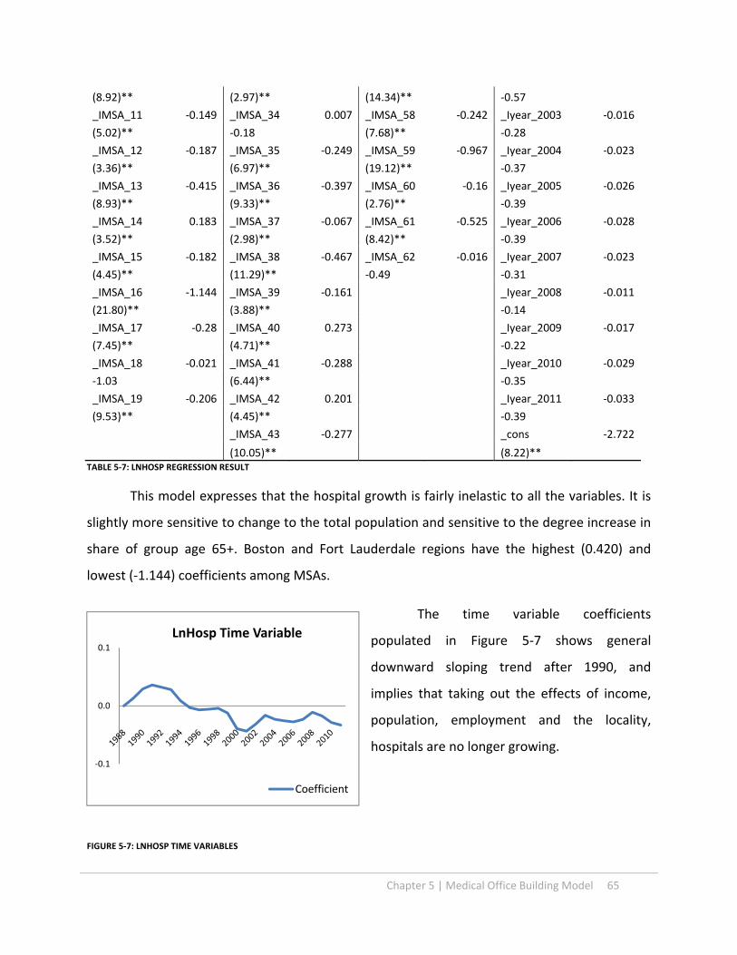
Chapter 5 | Medical Office Building Model 65
(8.92)** (2.97)** (14.34)** ‐0.57
_IMSA_11 ‐0.149 _IMSA_34 0.007 _IMSA_58 ‐0.242 _Iyear_2003 ‐0.016
(5.02)** ‐0.18 (7.68)** ‐0.28
_IMSA_12 ‐0.187 _IMSA_35 ‐0.249 _IMSA_59 ‐0.967 _Iyear_2004 ‐0.023
(3.36)** (6.97)** (19.12)** ‐0.37
_IMSA_13 ‐0.415 _IMSA_36 ‐0.397 _IMSA_60 ‐0.16 _Iyear_2005 ‐0.026
(8.93)** (9.33)** (2.76)** ‐0.39
_IMSA_14 0.183 _IMSA_37 ‐0.067 _IMSA_61 ‐0.525 _Iyear_2006 ‐0.028
(3.52)** (2.98)** (8.42)** ‐0.39
_IMSA_15 ‐0.182 _IMSA_38 ‐0.467 _IMSA_62 ‐0.016 _Iyear_2007 ‐0.023
(4.45)** (11.29)** ‐0.49 ‐0.31
_IMSA_16 ‐1.144 _IMSA_39 ‐0.161 _Iyear_2008 ‐0.011
(21.80)** (3.88)** ‐0.14
_IMSA_17 ‐0.28 _IMSA_40 0.273 _Iyear_2009 ‐0.017
(7.45)** (4.71)** ‐0.22
_IMSA_18 ‐0.021 _IMSA_41 ‐0.288 _Iyear_2010 ‐0.029
‐1.03 (6.44)** ‐0.35
_IMSA_19 ‐0.206 _IMSA_42 0.201 _Iyear_2011 ‐0.033
(9.53)** (4.45)** ‐0.39
_IMSA_43 ‐0.277 _cons ‐2.722
(10.05)** (8.22)** TABLE 5‐7: LNHOSP REGRESSION RESULT
This model expresses that the hospital growth is fairly inelastic to all the variables. It is
slightly more sensitive to change to the total population and sensitive to the degree increase in
share of group age 65+. Boston and Fort Lauderdale regions have the highest (0.420) and
lowest (‐1.144) coefficients among MSAs.
The time variable coefficients
populated in Figure 5‐7 shows general
downward sloping trend after 1990, and
implies that taking out the effects of income,
population, employment and the locality,
hospitals are no longer growing.
FIGURE 5‐7: LNHOSP TIME VARIABLES
‐0.1
0.0
0.1
LnHosp Time Variable
Coefficient

66 Medical Office Building Model | Chapter 5
5.3.9 INDEPENDENT VARIABLES FOR HEALTH CARE EMPLOYMENT
Looking at the coefficients across health care employment models, each variable in the
log form has different implication to different sectors as listed in Table 5‐8. The percentage
change in population impact all sectors, and has the largest impact on the percentage change in
Labs. The coefficient 1.72 represent that with every 1 % increase in population, there is 1.72 %
increase in employment of medical and diagnostic laboratories. Employment per captia also has
significant impact on all sectors except hospitals, and office of others is the most sensitive to
the changes in employment per captia. The third significant influence is the share of group age
65+ to total population. It has positive impact on all sectors, and has the most considerable
impact on the office of the others for 1% increase in the share of group age 65+ brings 0.7 %
increase in offices of others.
On average, health care employment sectors are less sensitive to changes in income per
captia and the share of group age 45‐65. However, outpatient care centers are responsive to
the share of group age 45‐65, and medical and diagnostic laboratories are more sensitive to the
change in income per captia within health care employment sectors.
FIGURE 5‐8: COEFFICIENTS FOR HC EMPLY INDEPENDENT VARIABLES
In addition to the distinct elasticity pattern from each economic and demographic factor
to each sectors, trends derived from time variables of each model present considerable
differences. The time coefficients represent effects responding to time only, and they explain
influences that are not from other variables such as economic, population or aging. As Figure 5‐
9 shows, LnOut has the largest increase in time coefficient and LnHosp reached negative value
in 2011. LnDent’s time variables have stopped increasing since 2003 in contract to other sectors.
Coefficient LnPhy LnDent LnOther LnOut LnLabs LnHosp Average
LnEm_P 0.78072 0.37117 1.14910 0.12944 1.20687 ‐0.15064 0.58111
LnIn_P ‐0.32068 0.02180 ‐0.26294 ‐0.44901 ‐0.83213 0.08765 ‐0.29255
LnPop 0.95688 1.18014 0.69068 0.83533 1.72198 0.87901 1.04400
LnP4565_P ‐0.05524 0.07572 ‐0.81295 ‐1.49027 0.11803 0.15363 ‐0.33518
LnP65_P 0.03043 0.53196 0.74324 0.33981 0.25385 0.31185 0.36852
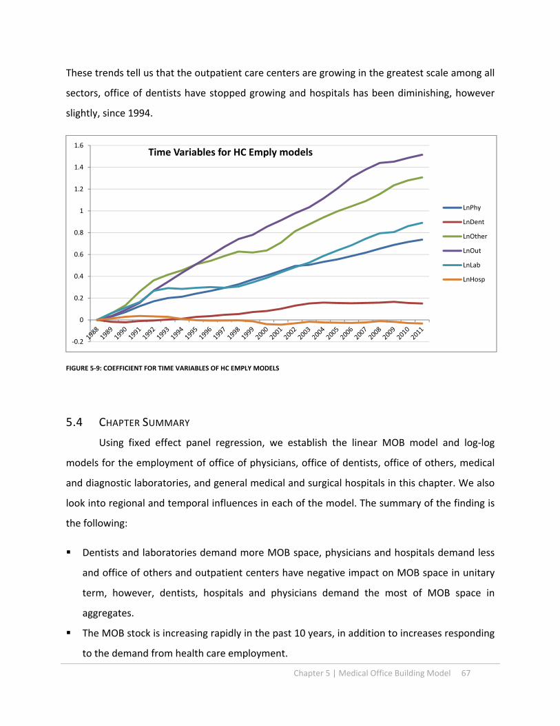
Chapter 5 | Medical Office Building Model 67
These trends tell us that the outpatient care centers are growing in the greatest scale among all
sectors, office of dentists have stopped growing and hospitals has been diminishing, however
slightly, since 1994.
FIGURE 5‐9: COEFFICIENT FOR TIME VARIABLES OF HC EMPLY MODELS
5.4 CHAPTER SUMMARY
Using fixed effect panel regression, we establish the linear MOB model and log‐log
models for the employment of office of physicians, office of dentists, office of others, medical
and diagnostic laboratories, and general medical and surgical hospitals in this chapter. We also
look into regional and temporal influences in each of the model. The summary of the finding is
the following:
Dentists and laboratories demand more MOB space, physicians and hospitals demand less
and office of others and outpatient centers have negative impact on MOB space in unitary
term, however, dentists, hospitals and physicians demand the most of MOB space in
aggregates.
The MOB stock is increasing rapidly in the past 10 years, in addition to increases responding
to the demand from health care employment.
‐0.2
0
0.2
0.4
0.6
0.8
1
1.2
1.4
1.6Time Variables for HC Emply models
LnPhy
LnDent
LnOther
LnOut
LnLab
LnHosp

68 Medical Office Building Model | Chapter 5
The office of physicians has been increasing growth rate and corresponsive to total
employment and population, however, it is inelastic to the share of group age 65+.
The growth in the office of dentist is slight and is sensitive to the growth of total population.
The employment of office of others is more sensitive to employment, corresponsive to
population, share of group age 65+, income per capita and decrease in share of group age
45‐65. Its growth is subtle.
The outpatient care center has the significant increase in growth rate, and is more elastic to
the decrease in share of group age 45‐65 to total population.
The employment of medical and diagnostic laboratories is sensitive to total population and
employment. The growth rate has been increasing subtly.
The employment of general medical and surgical hospitals is not growing. It is fairly inelastic
to employment, income and the share of group age 45‐65, but slightly more sensitive to
total population and the change in the share of group age 65+.

Chapter 6 | Forecasts 69
Chapter 6. FORECASTS
6.1 DEFINITION
In this chapter, we develop different scenarios for MOB forecasts in 2022. We test what
implications are for the MOB under hypotheses as follow: 1) the health care industry continue to
growth and MOB stays with the current development trend as the base case scenario; 2) the
health care industry continues to grow but MOB development trend slows down to the pre‐2002
development trend level, and 3) the worst case scenario is with the combination of the slow
growth for health care industry and the slow trend in the MOB development.
We have defined the relationship among all factors with the tier‐two model established in
the early chapter. We use the employment, income and population data in 2022 projected by
Moody’s corporation to build the data set for independent variables ( Table 2‐2, Xr ) in each of the
health care employment model (Equations 5‐2~5‐7). Location variables (IMSA_k ) are generated
with panel regression, and we develop values of time variables (Iyear_ i) for each model in 2022.
Referring to the average growth of Moody’s sectional health care employment data, we find time
variable coefficients for each model as the continuous growth trend scenario for health care
employment. In addition, we develop a slow growth scenario for health care employment by
lowering the projected value of the time variable.
With the health care employment data as variables (Table 2‐1, Xi) established and location
variables (IMSA_k ) extracted from panel regressions, we construct the coefficient of time variable
in 2022 for MOB model ( Equation 5‐1). We develop different trend lines via running the
regression with coefficients of time variables, and project two time variables representing positive
trend and conservative trends for MOB in 2022.
With these three scenarios, we have a range of the MOB demand corresponding to each
MSA for the next 10 years, and we analyze these outcomes to find the best and the worst markets
for MOB.

70 Forecasts | Chapter 6
6.2 FORECAST FOR HEALTH CARE EMPLOYMENT
In Chapter 5, we establish models (Equation 5‐2~5‐7) for office of physicians, office of
dentists, office of others, outpatient care center, medical and diagnostic laboratories, and general
medical and surgical hospitals using independent variables of employment per capita, income per
captia, total population and fractions of age group 45‐65 and 65+ to total population in each MSAs.
We also obtained the economic and demographic data in 2022 from Moody’s described in Chapter
4, and apply the data to construct forecasts for each sector of health care employment in this
section. With sectors of health care employment, we compare the health care trends, composition
and practice changes in aggregates and across markets.

Chapter 6 | Forecasts 71
6.2.1 OFFICE OF PHYSICIANS
FIGURE 6‐1: OFFICES OF PHYSICIANS IN 2022
Using data of office of physicians projected by Moody’s, we established that the average
growth rate for offices of physicians from 2011 to 2022 is at 25.76%. We find the time variable
value of 0.914 for the Equation 5‐2 applied to all MSAs creates the average growth rate at 25.76%.
Figure 6‐1 is the plot of the continuous growth scenario for office of physician in 2022. Like 2011,
the MSA have the largest number and
the lowest employment numbers of
offices of physicians are Los Angeles
and Albuquerque, with 96.15 and 6.381
in 2022.
We see the continuous increase
in time variables in Figure 6‐2 after
constructing the linear relationship. For
the slow growth scenario, we assume
the trend of office of physician growth
will slow down by 50% after 2011 by
cutting the slop in half, and we reach a
1 All employment number presented in this paper is in the unit of thousands
‐40%
‐20%
0%
20%
40%
60%
80%
100%
120%
‐40
‐20
0
20
40
60
80
100
120
Albany
Albuquerque
Atlanta
Austin
Baltimore
Boston
Charlotte
Chicago
Cincinnati
Cleveland
Columbus
Dallas
Den
ver
Detroit
Edison
Fort Lauderdale
Fort W
orth
Hartford
Honolulu
Houston
Indianapolis
Jacksonville
Kansas City
Las Vegas
Long Island
Los Angeles
Louisville
Mem
phis
Miami
Milw
aukee
Minneapolis
Nashville
New
York
New
ark
Norfolk
Oakland
Oklahoma City
Orange County
Orlando
Philadelphia
Phoenix
Pittsburgh
Portland
Raleigh
Richmond
Riverside
Sacram
ento
Salt Lake City
San Antonio
San Diego
San Francisco
San Jose
Seattle
St. Louis
Stam
ford
Tampa
Tucson
Tulsa
Ventura
Washington, D
CWest Palm Beach
Wilm
ington
Offices of Physicians in 2022 (in 1000s)
Physician 2011 difference Projected Growth Rate
0
0.1
0.2
0.3
0.4
0.5
0.6
0.7
0.8
0.9
1 InPhy Time Variable
historical
Continuous Growth
slow growth
FIGURE 6‐2: LNPHY TIME VARIABLES

72 Forecasts | Chapter 6
time variable value at 0.830. We apply these two time variable values representing lyear 2022 in
two scenarios, with individual IMSA and projected economic and demographic data for each MSA,
and introduce the data for offices of physicians in 20222 presented in Figure 6‐3.
In two scenarios plotted in Figure 6‐3, Los Angles has the highest number of office of
physicians and most increase of 17.23 and 8.84 (thousands) under the continuous growth and
slow growth scenarios, and Norfolk has lost the most of 6.4 and 5.24 (in thousands) under
continuous growth and slower trend.
FIGURE 6‐3: OFFICE OF PHYSICIANS IN CONTINUOUS AND SLOW GROWTH IN 2022
The MSA with largest increase and largest decrease in percentages for offices of physicians
are Sacramento (continuous growth: 74.5%, slow growth: 58.9%) and Norfolk (continuous growth:
‐46.52%, slow growth: ‐36.86%). The growth in Sacramento comes from moderate growth in
employment per captia and moderate growth in population, and Norfolk’s location coefficient and
small population growth contribute the most to its lost. Compare to the continuous growth
scenario, the average growth rate from 2011 to 2022 for slow growth scenario is at the lower level
of 14.5%.
6.2.2 OFFICE OF DENTISTS
2 See Appendix H1 for the full data
‐120%
‐60%
0%
60%
120%
180%
240%
300%
‐40
‐20
0
20
40
60
80
100
Albany
Albuquerque
Atlanta
Austin
Baltimore
Boston
Charlotte
Chicago
Cincinnati
Cleveland
Columbus
Dallas
Den
ver
Detroit
Edison
Fort Lauderdale
Fort W
orth
Hartford
Honolulu
Houston
Indianapolis
Jacksonville
Kansas City
Las Vegas
Long Island
Los Angeles
Louisville
Mem
phis
Miami
Milw
aukee
Minneapolis
Nashville
New
York
New
ark
Norfolk
Oakland
Oklahoma City
Orange County
Orlando
Philadelphia
Phoenix
Pittsburgh
Portland
Raleigh
Richmond
Riverside
Sacram
ento
Salt Lake City
San Antonio
San Diego
San Francisco
San Jose
Seattle
St. Louis
Stam
ford
Tampa
Tucson
Tulsa
Ventura
Washington, D
C
West Palm Beach
Wilm
ington
Offices of Physicians in 2022 (in 1000s)
Continuous growth Slow growth
Growth Rate_Continuous Growth Growth Rate_Slow Growth

Chapter 6 | Forecasts 73
FIGURE 6‐4: OFFICES OF DENTISTS
We establish the time variable value at 0.12 for the year 2002 to simulate the slowly
decreasing trend. With projected economic and population data, it results average of 30.6%
increase in employment in dentists’ offices across MSAs as illustrated in Figure 6‐4. The MSA has
the largest and least number for the employment of offices of dentists is Los Angeles, and the one
has the least is Wilmington in both 2011 and 2022. Los Angeles has 29.5 and 34.4, and wilmington
has 2.0 and 2.3 thousands employment of offices of dentists in the year of 2011 and 2022
respectively.
In Figure 6‐5, the continuous trend
shown is at a gentle downward slope from
2011 to 2022. We set the value for the slow
trend in 2022 at 0.1 to simulate steeper
decline as the slow trend.
The results of two different scenarios
with continuous and slow trend time
variable values are demonstrated in Figure
6‐6, Los Angles has the highest number of
office of dentists and most increase of 9.5
and 8.8 (in thousands) under the continuous
‐40%
‐20%
0%
20%
40%
60%
80%
100%
‐20
‐10
0
10
20
30
40
50
Albany
Albuquerque
Atlanta
Austin
Baltimore
Boston
Charlotte
Chicago
Cincinnati
Cleveland
Columbus
Dallas
Den
ver
Detroit
Edison
Fort Lauderdale
Fort W
orth
Hartford
Honolulu
Houston
Indianapolis
Jacksonville
Kansas City
Las Vegas
Long Island
Los Angeles
Louisville
Mem
phis
Miami
Milw
aukee
Minneapolis
Nashville
New
York
New
ark
Norfolk
Oakland
Oklahoma City
Orange County
Orlando
Philadelphia
Phoenix
Pittsburgh
Portland
Raleigh
Richmond
Riverside
Sacram
ento
Salt Lake City
San Antonio
San Diego
San Francisco
San Jose
Seattle
St. Louis
Stam
ford
Tampa
Tucson
Tulsa
Ventura
Washington, D
CWest Palm Beach
Wilm
ington
Offices of Dentists in 2022 (1000s)
Dentists in 2011 Difference Projected growth rate
FIGURE 6‐6: LNDENT TIME VARIABLES
‐0.05
0
0.05
0.1
0.15
0.2
1989
1991
1993
1995
1997
1999
2001
2003
2005
2007
2009
2011
2013
2015
2017
2019
2021
LnDent Time Variables historical
continuoustrendslow trend
FIGURE 6‐5 : LNDENT TIME VARIABLES

74 Forecasts | Chapter 6
and slow trend scenario, and Norfolk has the most loss of 1.45 and 1.52 (in thousands) under base
case and slow trend scenarios.
The MSAs with largest increase and largest decrease in percentages for office of dentists
are Tucson (continuous trend: 95.1%, slow trend scenario: 91.3%) and Norfolk (continuous trend: ‐
29.0%, slow trend scenario: ‐30.4%). The growth in Tucson comes from moderate growth in
population and growth in the share of group 65+, and Norfolk’s small population growth and
location coefficient contribute the most to its lost. Comparing to the continuous growth scenario,
the average growth rate from 2011 to 2022 in slow growth scenario is at the lower level of 28.0%3.
FIGURE 6‐6: OFFICE OF DENTISTS IN CONTINUOUS AND SLOW GROWTH IN 2022
3 See Appendix H2 for full data
‐80%
‐30%
20%
70%
120%
‐20
‐10
0
10
20
30
40
Albany
Albuquerque
Atlanta
Austin
Baltimore
Boston
Charlotte
Chicago
Cincinnati
Cleveland
Columbus
Dallas
Denver
Detroit
Edison
Fort Lauderdale
Fort W
orth
Hartford
Honolulu
Houston
Indianapolis
Jacksonville
Kansas City
Las Vegas
Long Island
Los Angeles
Louisville
Memphis
Miami
Milw
aukee
Minneapolis
Nashville
New York
Newark
Norfolk
Oakland
Oklahoma City
Orange County
Orlando
Philadelphia
Phoen
ix
Pittsburgh
Portland
Raleigh
Richmond
Riverside
Sacram
ento
Salt Lake City
San Antonio
San Diego
San Francisco
San Jose
Seattle
St. Louis
Stam
ford
Tampa
Tucson
Tulsa
Ven
tura
Washington, D
C
West Palm Beach
Wilm
ington
Offices of Dentists in 2022 (1000s)
continuous trend Slow trend growth rate_continuous growth rate_slow

Chapter 6 | Forecasts 75
6.2.3 OFFICE OF OTHERS
FIGURE 6‐7: OFFICE OF OTHER HEALTH PRACTITIONERS IN 2022
Repeating the process, we establish that the average growth rate for offices of others from
2011 to 2022 is at 50.9%. We find the time variable value of 1.54 in the Equation 5‐4 that will
produce the average growth rate of 50.9% across MSAs. Figure 6‐7 is the plot for projected offices
of dentists in 2022. It shows that in 2011, Chicago has the most of offices of other health
practitioners but New York will have the most in 2022.
With the time variable value at
1.54, we reconstruct the linear
relationship in time variables, and we can
see the flatten trend in growth rate in
Figure 6‐8. For slow growth scenario, we
assume the decreasing in growth rate for
office of dentists will slow down by 50%
after 2011, and we reach a time variable
value at 1.37.
The two different scenarios are
plotted in Figure 6‐9, Los Angeles has the
highest most increase in office of others at
‐20%
30%
80%
130%
180%
‐4
1
6
11
16
21
26
31
36
Albany
Albuquerque
Atlanta
Austin
Baltimore
Boston
Charlotte
Chicago
Cincinnati
Cleveland
Columbus
Dallas
Den
ver
Detroit
Edison
Fort Lauderdale
Fort W
orth
Hartford
Honolulu
Houston
Indianapolis
Jacksonville
Kansas City
Las Vegas
Long Island
Los Angeles
Louisville
Mem
phis
Miami
Milw
aukee
Minneapolis
Nashville
New
York
New
ark
Norfolk
Oakland
Oklahoma City
Orange County
Orlando
Philadelphia
Phoenix
Pittsburgh
Portland
Raleigh
Richmond
Riverside
Sacram
ento
Salt Lake City
San Antonio
San Diego
San Francisco
San Jose
Seattle
St. Louis
Stam
ford
Tampa
Tucson
Tulsa
Ventura
Washington, D
CWest Palm Beach
Wilm
ington
Office of Other Health Practitioners in 2022 (in 1000s)
2011 difference growth rate
FIGURE 6‐8:LNOTHERS TIME VARIABLES
0
0.2
0.4
0.6
0.8
1
1.2
1.4
1.6
1989
1991
1993
1995
1997
1999
2001
2003
2005
2007
2009
2011
2013
2015
2017
2019
2021
LnOthers Time Variable
historical
Continuousgrowthslow growth

76 Forecasts | Chapter 6
9.44 and 11.11 (in thousands) under the continuous growth and slow growth, and Chicago and
Norfolk has the most loss of 1.59 and 0.59 (in thousands) respectively under the continuous
growth and slow growth scenarios.
The MSAs with largest increase and largest decrease in percentages for office of others are
San Francisco (continuous growth: 145.4%, slow growth scenario: 130.1%) and Norfolk
(continuous growth: ‐20.22%, slow growth scenario: ‐14.94%). The growth in San Francisco comes
from strong growth in employment and growth in the share of group 65+, and Norfolk’s location
coefficient, small employment growth and smaller share in 65+ are some obvious reasons for its
lost. Compare to the continuous growth scenario, the average growth rate for office of others
from 2011 to 2022 in slow growth is at lower level at 42.51%4.
FIGURE 6‐9: OFFICE OF OTHER HEALTH PRACTITIONERS IN CONTINUOUS AND SLOW GROWTH
4 See Appendix H3 for the full data
‐0.2
0
0.2
0.4
0.6
0.8
1
1.2
1.4
1.6
1.8
‐5
0
5
10
15
20
25
30
35
40
45
Albany
Albuquerque
Atlanta
Austin
Baltimore
Boston
Charlotte
Chicago
Cincinnati
Cleveland
Columbus
Dallas
Den
ver
Detroit
Edison
Fort Lauderdale
Fort W
orth
Hartford
Honolulu
Houston
Indianapolis
Jacksonville
Kansas City
Las Vegas
Long Island
Los Angeles
Louisville
Mem
phis
Miami
Milw
aukee
Minneapolis
Nashville
New
York
New
ark
Norfolk
Oakland
Oklahoma City
Orange County
Orlando
Philadelphia
Phoenix
Pittsburgh
Portland
Raleigh
Richmond
Riverside
Sacram
ento
Salt Lake City
San Antonio
San Diego
San Francisco
San Jose
Seattle
St. Louis
Stam
ford
Tampa
Tucson
Tulsa
Ventura
Washington, D
CWest Palm Beach
Wilm
ington
Office of Other Health Practitioners in 2022 (in 1000s)
Scenario 1 Base case Growth Rate Scenario 1 Growth rate Base case

Chapter 6 | Forecasts 77
6.2.4 OUTPATIENT CARE CENTERS
FIGURE 6‐10: OUTPATIENT CARE CENTERS IN 2022
Using health care employment data projected by Moody’s, we established that the average
growth rate for outpatient care center from 2011 to 2022 is at 55.2%. We find the time variable
value of 1.78 for Equation 5‐5 that will produce the average growth rate for 62 MSAs at 50.9%.
Figure 6‐10 is populated with the employment of outpatient care centers in 2022. It
indicates Los Angeles will take over New York and become the MSA has the most employment for
outpatient care centers in 2022.
With the time variable value at 1.78,
we reconstruct the linear relationship in time
variables, and we can see the increases in
growth rate in Figure 6‐11. For slow growth
scenario, we assume the increasing in growth
rate for outpatient care center will slow down
by 50% after 2011, and we calculate that time
variable value at 1.64 that satisfies the
equation.
Demonstrated in Figure 6‐12
populated with two scenarios, Los Angeles has
‐50%
50%
150%
250%
350%
450%
‐5
5
15
25
35
45
Albany
Albuquerque
Atlanta
Austin
Baltimore
Boston
Charlotte
Chicago
Cincinnati
Cleveland
Columbus
Dallas
Den
ver
Detroit
Edison
Fort Lauderdale
Fort W
orth
Hartford
Honolulu
Houston
Indianapolis
Jacksonville
Kansas City
Las Vegas
Long Island
Los Angeles
Louisville
Mem
phis
Miami
Milw
aukee
Minneapolis
Nashville
New
York
New
ark
Norfolk
Oakland
Oklahoma City
Orange County
Orlando
Philadelphia
Phoenix
Pittsburgh
Portland
Raleigh
Richmond
Riverside
Sacram
ento
Salt Lake City
San Antonio
San Diego
San Francisco
San Jose
Seattle
St. Louis
Stam
ford
Tampa
Tucson
Tulsa
Ventura
Washington, D
CWest Palm Beach
Wilm
ington
Outpatient Care Centers in 2022
Difference 2011 Projected growth rate
0
0.2
0.4
0.6
0.8
1
1.2
1.4
1.6
1.8
2
1989
1991
1993
1995
1997
1999
2001
2003
2005
2007
2009
2011
2013
2015
2017
2019
2021
LnOut Time Variable
historical
continuousgrowthslow growth
FIGURE 6‐11:LNOUT TIME VARIABLES

78 Forecasts | Chapter 6
the highest most increase in office of others at 8.68 and 12.87 (in thousands) under the
continuous growth and slow growth scenarios, and Oakland has the most loss of 5.57 and 4.00 (in
thousands) for outpatient care center for the two.
FIGURE 6‐12: OUTPATIENT CARE CENTERS
The MSAs with largest increase and largest decrease in percentages for outpatient care
centers are Norfolk (Base case: 437.4%, Slow growth scenario: 371.2%) and San Jose (Base case: ‐
28.7%, slow growth scenario: ‐37.4%). Norfolk’s location coefficient, small income growth and
smaller change in share in 45‐65 are some reasons for its growth. San Jose’s location coefficient
and small population growth cause the loss for outpatient care centers. Compare to the base case
scenario, the average growth rate for office of others from 2011 to 2022 in growth scenario is at
lower level of 36.09%5.
5 See Appendix H4 for the full data
‐0.5
0.5
1.5
2.5
3.5
4.5
‐5
5
15
25
35
45
Albany
Albuquerque
Atlanta
Austin
Baltimore
Boston
Charlotte
Chicago
Cincinnati
Cleveland
Columbus
Dallas
Den
ver
Detroit
Edison
Fort Lauderdale
Fort W
orth
Hartford
Honolulu
Houston
Indianapolis
Jacksonville
Kansas City
Las Vegas
Long Island
Los Angeles
Louisville
Mem
phis
Miami
Milw
aukee
Minneapolis
Nashville
New
York
New
ark
Norfolk
Oakland
Oklahoma City
Orange County
Orlando
Philadelphia
Phoenix
Pittsburgh
Portland
Raleigh
Richmond
Riverside
Sacram
ento
Salt Lake City
San Antonio
San Diego
San Francisco
San Jose
Seattle
St. Louis
Stam
ford
Tampa
Tucson
Tulsa
Ventura
Washington, D
CWest Palm Beach
Wilm
ington
Outpatient Care Centers in 2022 (In 1000s)
slow growth continuous growth growth rate_continuous growth growth rate_slow growth
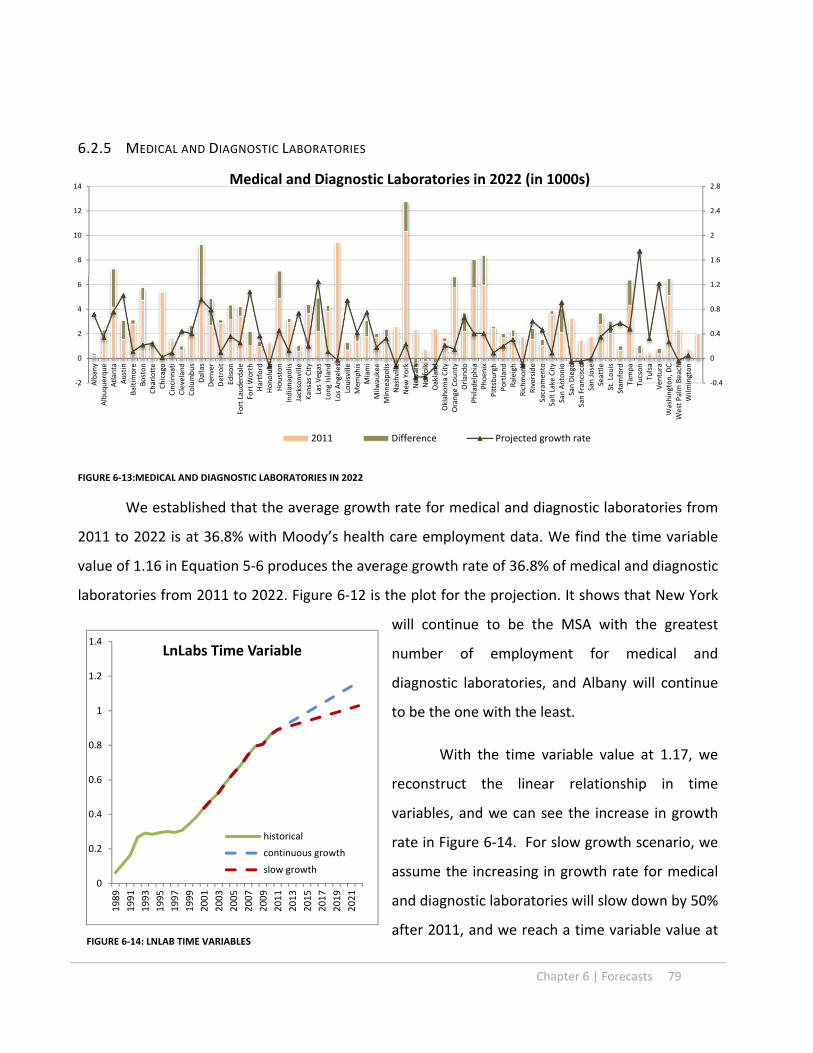
Chapter 6 | Forecasts 79
6.2.5 MEDICAL AND DIAGNOSTIC LABORATORIES
FIGURE 6‐13:MEDICAL AND DIAGNOSTIC LABORATORIES IN 2022
We established that the average growth rate for medical and diagnostic laboratories from
2011 to 2022 is at 36.8% with Moody’s health care employment data. We find the time variable
value of 1.16 in Equation 5‐6 produces the average growth rate of 36.8% of medical and diagnostic
laboratories from 2011 to 2022. Figure 6‐12 is the plot for the projection. It shows that New York
will continue to be the MSA with the greatest
number of employment for medical and
diagnostic laboratories, and Albany will continue
to be the one with the least.
With the time variable value at 1.17, we
reconstruct the linear relationship in time
variables, and we can see the increase in growth
rate in Figure 6‐14. For slow growth scenario, we
assume the increasing in growth rate for medical
and diagnostic laboratories will slow down by 50%
after 2011, and we reach a time variable value at
‐0.4
0
0.4
0.8
1.2
1.6
2
2.4
2.8
‐2
0
2
4
6
8
10
12
14
Albany
Albuquerque
Atlanta
Austin
Baltimore
Boston
Charlotte
Chicago
Cincinnati
Cleveland
Columbus
Dallas
Den
ver
Detroit
Edison
Fort Lauderdale
Fort W
orth
Hartford
Honolulu
Houston
Indianapolis
Jacksonville
Kansas City
Las Vegas
Long Island
Los Angeles
Louisville
Mem
phis
Miami
Milw
aukee
Minneapolis
Nashville
New
York
New
ark
Norfolk
Oakland
Oklahoma City
Orange County
Orlando
Philadelphia
Phoenix
Pittsburgh
Portland
Raleigh
Richmond
Riverside
Sacram
ento
Salt Lake City
San Antonio
San Diego
San Francisco
San Jose
Seattle
St. Louis
Stam
ford
Tampa
Tucson
Tulsa
Ventura
Washington, D
CWest Palm Beach
Wilm
ington
Medical and Diagnostic Laboratories in 2022 (in 1000s)
2011 Difference Projected growth rate
0
0.2
0.4
0.6
0.8
1
1.2
1.4
1989
1991
1993
1995
1997
1999
2001
2003
2005
2007
2009
2011
2013
2015
2017
2019
2021
LnLabs Time Variable
historical
continuous growth
slow growth
FIGURE 6‐14: LNLAB TIME VARIABLES
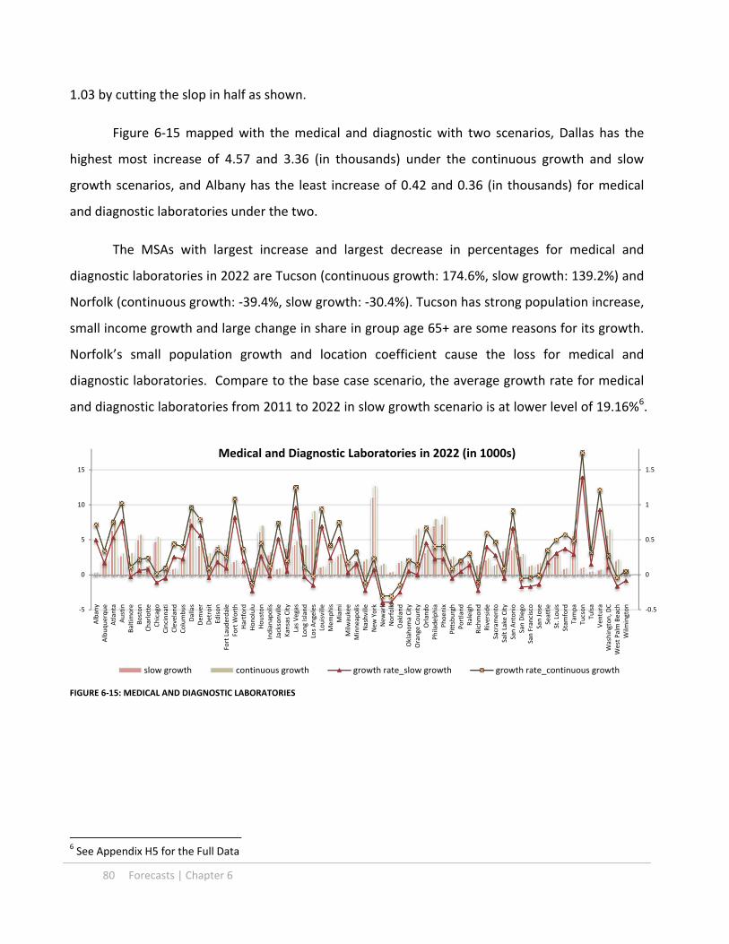
80 Forecasts | Chapter 6
1.03 by cutting the slop in half as shown.
Figure 6‐15 mapped with the medical and diagnostic with two scenarios, Dallas has the
highest most increase of 4.57 and 3.36 (in thousands) under the continuous growth and slow
growth scenarios, and Albany has the least increase of 0.42 and 0.36 (in thousands) for medical
and diagnostic laboratories under the two.
The MSAs with largest increase and largest decrease in percentages for medical and
diagnostic laboratories in 2022 are Tucson (continuous growth: 174.6%, slow growth: 139.2%) and
Norfolk (continuous growth: ‐39.4%, slow growth: ‐30.4%). Tucson has strong population increase,
small income growth and large change in share in group age 65+ are some reasons for its growth.
Norfolk’s small population growth and location coefficient cause the loss for medical and
diagnostic laboratories. Compare to the base case scenario, the average growth rate for medical
and diagnostic laboratories from 2011 to 2022 in slow growth scenario is at lower level of 19.16%6.
FIGURE 6‐15: MEDICAL AND DIAGNOSTIC LABORATORIES
6 See Appendix H5 for the Full Data
‐0.5
0
0.5
1
1.5
‐5
0
5
10
15
Albany
Albuquerque
Atlanta
Austin
Baltimore
Boston
Charlotte
Chicago
Cincinnati
Cleveland
Columbus
Dallas
Den
ver
Detroit
Edison
Fort Lauderdale
Fort W
orth
Hartford
Honolulu
Houston
Indianapolis
Jacksonville
Kansas City
Las Vegas
Long Island
Los Angeles
Louisville
Mem
phis
Miami
Milw
aukee
Minneapolis
Nashville
New
York
New
ark
Norfolk
Oakland
Oklahoma City
Orange County
Orlando
Philadelphia
Phoenix
Pittsburgh
Portland
Raleigh
Richmond
Riverside
Sacram
ento
Salt Lake City
San Antonio
San Diego
San Francisco
San Jose
Seattle
St. Louis
Stam
ford
Tampa
Tucson
Tulsa
Ventura
Washington, D
CWest Palm Beach
Wilm
ington
Medical and Diagnostic Laboratories in 2022 (in 1000s)
slow growth continuous growth growth rate_slow growth growth rate_continuous growth

Chapter 6 | Forecasts 81
6.2.6 GENERAL MEDICAL AND SURGICAL HOSPITALS
FIGURE 6‐16: MEDICAL AND SURGICAL HOSPITAL EMPLOYMENT IN 2022
We use the time variable value of ‐0.04 in the Equation 6‐7 that creates the average
growth rate for hospital employment at 25.4%. Figure 6‐16 is the plot of the continuous growth
for general medical and surgical hospitals in 2022. It shows that New York is the largest market for
medical and surgical hospital employment and Ventura is the smallest across MSAs, both in 2011
and 2022. In 2011, New York had 195.1 and Ventura had 5.4; in 2022, New York has 217.0 and
Ventura has 6.1.
Although the value of the time
coefficient was on decreasing trend, we believe
that the decreasing rate will become benign. In
Figure 6‐17, the continuous trend shown is at
a gentle downward slope from 2011 to 2022.
We set the value for the slow trend in 2022 at ‐
0.06 to simulate steeper decline as the slow
trend.
Figure 6‐19 illustrates the employment
for general medical and surgical hospitals with
two scenarios. Los Angeles has the most
increase of 33.0 and 29.3 (in thousands) under
‐50%
0%
50%
100%
150%
200%
250%
‐50
0
50
100
150
200
250
Albany
Albuquerque
Atlanta
Austin
Baltimore
Boston
Charlotte
Chicago
Cincinnati
Cleveland
Columbus
Dallas
Denver
Detroit
Edison
Fort Lauderdale
Fort W
orth
Hartford
Honolulu
Houston
Indianapolis
Jacksonville
Kansas City
Las Vegas
Long Island
Los Angeles
Louisville
Memphis
Miami
Milw
aukee
Minneapolis
Nashville
New York
Newark
Norfolk
Oakland
Oklahoma City
Orange County
Orlando
Philadelphia
Phoen
ix
Pittsburgh
Portland
Raleigh
Richmond
Riverside
Sacram
ento
Salt Lake City
San Antonio
San Diego
San Francisco
San Jose
Seattle
St. Louis
Stam
ford
Tampa
Tucson
Tulsa
Ven
tura
Washington, D
C
West Palm Beach
Wilm
ington
Medical and Surgical Hospital Employment in 2022 (in 1000s)
Difference 2011 Projected growth rate
‐0.08
‐0.06
‐0.04
‐0.02
0
0.02
0.04
0.06
1989
1991
1993
1995
1997
1999
2001
2003
2005
2007
2009
2011
2013
2015
2017
2019
2021
lnHosp Time Variable slow trend
Continuoustrend
historical
FIGURE 6‐17: LNHOSP TIME VARIABLES

82 Forecasts | Chapter 6
the continuous and slow trend scenarios, and Cleveland has the most decrease of 5.5 and 6.6 (in
thousands) for continuous and slow trend scenarios.
The MSAs with largest increase and largest decrease in percentages for general medical
and surgical hospitals from 2011 to 2022 are Tucson (continuous trend: 168.9%, slow trend:
163.6%) and Long Island (continuous trend: ‐9.3%, slow trend: ‐11.11%). Tucson has strong
population increase and high location coefficient compare to other MSAs. Long Island’s small
population growth causes the loss for general medical and surgical hospitals. Compare to the
continuous trend scenario, the average growth rate for general medical and surgical hospitals
from 2011 to 2022 in slow trend scenario is at higher level of 22.9%7.
FIGURE 6‐18: GENERAL MEDICAL AND SURGICAL HOSPITAL EMPLOYMENT CONTINUOUS AND SLOW TRENDS
7 See Appendix H6 for the full data
‐25%
25%
75%
125%
175%
225%
275%
‐25
25
75
125
175
225
275
Albany
Albuquerque
Atlanta
Austin
Baltimore
Boston
Charlotte
Chicago
Cincinnati
Cleveland
Columbus
Dallas
Denver
Detroit
Edison
Fort Lauderdale
Fort W
orth
Hartford
Honolulu
Houston
Indianapolis
Jacksonville
Kansas City
Las Vegas
Long Island
Los Angeles
Louisville
Memphis
Miami
Milw
aukee
Minneapolis
Nashville
New York
Newark
Norfolk
Oakland
Oklahoma City
Orange County
Orlando
Philadelphia
Phoen
ix
Pittsburgh
Portland
Raleigh
Richmond
Riverside
Sacram
ento
Salt Lake City
San Antonio
San Diego
San Francisco
San Jose
Seattle
St. Louis
Stam
ford
Tampa
Tucson
Tulsa
Ven
tura
Washington, D
C
West Palm Beach
Wilm
ington
General Medical and Surgical Hopital Employment in 2022 (in 1000s)
slow trend continuous trend growth rate_slow trend growth rate_continuous

Chapter 6 | Forecasts 83
6.2.7 HEALTH CARE EMPLOYMENT IN 2022
We incorporate the variables of income, employment, population, shares of age 45‐65 and
65+ into our models, and forecast the individual health care employment sectors. In year 2022, we
estimate that the growth in total health care employment8 will continue to out‐pace the
population, employment and the age group 45‐65 as shown in Figure 6‐209. The group age 65+
continues to growth at great rate. The nominal income per captia growth is also projected to
continue. Our forecasts for health care employment, however, is at lower growth rate than
Moody’s. We estimate that the total health care employment will be 6636.1710 , close to Moody’s
projection at 6611.75, for the continuous trends in all sectors, and it will be 6358.8910 for the slow
growth scenario.
The average growth rate is 28.1% for the continuous growth and 22.6% for the slow
growth case, and 26.4% for Moody’s. The differences in health care employment growth in total
again are presented in the Figure 6‐21. Tucson has the highest growth rates (continuous growth:
8 Excluding social assistance 9 See Appendix I 10 All employment numbers presented in this paper are in the unit of thousands
1
1.05
1.1
1.15
1.2
1.25
1.3
1.35
1.4
1.45
1.5
2011 2012 2013 2014 2015 2016 2017 2018 2019 2020 2021 2022
Growth Index Base on 2011
slow growth
continuous growth
Moody's
pop
45‐65
65+
income per captia
Emply per captia
FIGURE 6‐19: INCOME, EMPLOYMENT, POPULATION AND HEALTH CARE GROWTH INDEX

84 Forecasts | Chapter 6
102.2%; Slow growth: 95.8%) and Cleveland has the lowest growth rate in total health care
employment (continuous growth: 5.7%; slow growth: 2.3%)
FIGURE 6‐20:HEALH CARE EMPLOYMENT 2022
Looking at health care employment sectional shifts in Figure 6‐12, all cases indicate loss of
shares of hospital employment, and gains of shares of outpatient care centers and office of others.
Under the slow growth scenario, share of the office of dentists is at 10.3%, the largest share across
three scenarios; and under the continuous trend scenario, the office of physicians is at 24.8%, less
than the share in 2011. This indicates physicians’ offices are not increasing as fast as other
professional services under this scenario. These differences in shifts among these cases come from
the speed of developing trends represented by time variables in each of the models. Similarly,
Moody’s also projected the shift in health care employment11. All scenarios demonstrate the
continuous shift for health care workforce from hospital setting to other types of medical practices.
11 See Appendix J for projections
‐10%
10%
30%
50%
70%
90%
110%
‐50
50
150
250
350
450
550
Albany
Albuquerque
Atlanta
Austin
Baltimore
Boston
Charlotte
Chicago
Cincinnati
Cleveland
Columbus
Dallas
Denver
Detroit
Edison
Fort Lauderdale
Fort W
orth
Hartford
Honolulu
Houston
Indianapolis
Jacksonville
Kansas City
Las Vegas
Long Island
Los Angeles
Louisville
Memphis
Miami
Milw
aukee
Minneapolis
Nashville
New York
Newark
Norfolk
Oakland
Oklahoma City
Orange County
Orlando
Philadelphia
Phoen
ix
Pittsburgh
Portland
Raleigh
Richmond
Riverside
Sacram
ento
Salt Lake City
San Antonio
San Diego
San Francisco
San Jose
Seattle
St. Louis
Stam
ford
Tampa
Tucson
Tulsa
Ven
tura
Washington, D
C
West Palm Beach
Wilm
ington
Health Care Employment in 2022
Continue growth slow growth growth rate growth rate‐slow

Chapter 6 | Forecasts 85
Figure 6‐23 depicts the shift in all sectors for individual MAS in the continuous trend case.
The shift in medical practice is different considerably across MSAs. Overall, the MAS with the most
stable in health care employment composition is Raleigh, and the most volatile is Norfolk in the
continuous growth scenario. Norfolk lose the most shares in office of physicians (‐14.4%) and
offices of dentists (‐4.34%), but gains the most share in outpatient care centers (+ 14.3%). The
most share gain in office of physicians happens in Sacramento at 7.03 %, most share loss in Tucson
at ‐15.7%. San Jose, San Francisco, Las Vegas and Tuscan has the most increased shares in office of
dentists (2.73%), office of others (4.43%), medical and diagnostic laboratories ( 2.70%), and
general medical and surgical hospitals (14.62 %).
25.4%
9.6%
7.4%3.1%7.0%
47.6%
2011
25.4%
9.2%
9.0%
3.4%
8.7%
44.3%
Moody's
24.8%
9.8%
8.6%
3.2%
8.2%
45.3%
Continuous
23.6%
10.3%
8.4%2.9%
7.5%
47.3%
Slow
physician
dent
others
labs
outpat
hosp
FIGURE 6‐21:HEALTH CARE EMPLOYMENT COMPOSITION
Health Care Employment Composition in 2022

86 Forecasts | Chapter 6
In the slow trend case, Tucson and Austin are the most volatile and stable areas in health
care employment composition. The same set of MSAs have the most gains and losses but with
lesser differences.
FIGURE 6‐22: FRACTIONAL CHANGES IN HEALTH CARE EMPLOYMENT, CONTINUOUS TREND 2011‐202212
12 See Appendix K for the full data
‐20%
‐15%
‐10%
‐5%
0%
5%
10%
15%
20%
Fractional Changes in Health Care Employment Sectors from 2011 to 2022Continuous Trend Projection
Physician Dentists Others
Labs Outpatient Hospitals
‐20%
‐15%
‐10%
‐5%
0%
5%
10%
15%
20%
‐20%
‐15%
‐10%
‐5%
0%
5%
10%
15%
20%

Chapter 6 | Forecasts 87
FIGURE 6‐23: FRACTIONAL CHANGES IN HEALTH CARE EMPLOYMENT, SLOW TREND 2011‐202212
‐20%
‐15%
‐10%
‐5%
0%
5%
10%
15%
20%
Fractional Changes in Health Care Employment Sectors from 2011 to 2022Slow Trend Projection
Off_Phy Off_Dent Off_Others
Labs Outpatient Hosp
‐20%
‐15%
‐10%
‐5%
0%
5%
10%
15%
20%
‐20%
‐15%
‐10%
‐5%
0%
5%
10%
15%
20%

88 Forecasts | Chapter 6
6.3 FORECASTS FOR MEDICAL OFFICE BUILDING
For forecasting MOB stock in 2022, we have two sets of health care employment
forecasted with different scenarios in the prior section. We also develop two different scenarios
with MOB trends: positive trend and conservative trend. We combine these two scenarios with
the health care employment trends to create three scenarios to cast a possible range for future
MOB development in the next 10 years.
6.3.1 MOB TREND
FIGURE 6‐24: MOB TIME VARIABLES
We use MOB time variables to develop the trend line in order to set the time variable
coefficient in 2022. We can see the historical time variable curve describes the positive trend for
MOB development. Two obvious conditions presented here are the general growing trend from
1988 to 2002, and the rapid growth period from 2002 to 2008. In the context of the linear
Equation 5‐1, the trend line represents average 10.3 % annual growth in MOB stock from 1988 to
2002, and 21.1% annual growth from 2002 to 201113. The average annual growth from the time
variable from 1988 to 2011 is at 14.7%14.
13 See Table 5‐1 14 See Appendix L
‐50
0
50
100
150
200
250
1989
1991
1993
1995
1997
1999
2001
2003
2005
2007
2009
2011
2013
2015
2017
2019
2021
x 10000
MOB Time Variable ‐Conservative
Trend from 1988 to 2001
Historical
Projected
‐50
0
50
100
150
200
250
1989
1991
1993
1995
1997
1999
2001
2003
2005
2007
2009
2011
2013
2015
2017
2019
2021
x 10000
MOB Time Variable ‐Postive
Trend from 1988 to 2011
Historical
Projected

Chapter 6 | Forecasts 89
Even though the continuous extreme growth is unlikely to sustain in real estate market,
the upward development trend is in the evidence. We adopt this overall growing trend from 1988
to 2011 as the positive scenario and the slower grow trend from 1988 to 2002 as the conservative
scenario.
The slope for the future trend in the positive scenario is based on the regression result
from time variables from 1988 to 2011(Coefficient 61923.7 R²: 0.75). Starting with the time
variable value at 2011 using the same slop, we project the time variable value at 2206486 as the
positive MOB trend for scenario 1. Similarly, the conservative scenario’s trend line starting at 2011
with the slope developed from regression result from 1988 to 2002 (Coefficient 15107.8, R²: 0.77)
projects the time variable value at 1691510 in 2022, 23% lower than the positive trend. We will
use this value for scenario 2 and 3 for MOB forecasts.
6.3.2 MOB IN 2022
Combining with the projected data for health care employment, we use the MOB model
(5‐1) to develop forecasts in following three scenarios for MOB stock in 2022. Scenario 1) Positive
MOB trend and continue health care employment trend 2) conservative MOB trend and continue
health care employment trend; and 3) conservative MOB trend and slow health care employment
growth.
6.3.2.1 SCENARIO 1
FIGURE 6‐25: 2022 MOB STOCK – SCENARIO 1
‐10
0
10
20
30
40
50
Albany
Albuquerque
Atlanta
Austin
Baltimore
Boston
Charlotte
Chicago
Cincinnati
Cleveland
Columbus
Dallas
Den
ver
Detroit
Edison
Fort Lauderdale
Fort W
orth
Hartford
Honolulu
Houston
Indianapolis
Jacksonville
Kansas City
Las Vegas
Long Island
Los Angeles
Louisville
Mem
phis
Miami
Milw
aukee
Minneapolis
Nashville
New
York
New
ark
Norfolk
Oakland
Oklahoma City
Orange County
Orlando
Philadelphia
Phoenix
Pittsburgh
Portland
Raleigh
Richmond
Riverside
Sacram
ento
Salt Lake City
San Antonio
San Diego
San Francisco
San Jose
Seattle
St. Louis
Stam
ford
Tampa
Tucson
Tulsa
Ventura
Washington, D
C
West Palm Beach
Wilm
ington
2022 MOB stock Scenario 1
stock2011 additional

90 Forecasts | Chapter 6
The total increases for the MOB stock from 2022 to 2011 is at 147.95 million square feet
and average 28% growth rate across 62 MSA, indicating 2.5% average annual increases in MOB.
The MSA with the largest increase in square footage is Los Angeles at 7.2 million square feet and
the one with largest decrease by 2.2 million is Detroit. The MSA with largest increase in
percentage is Tucson (97.1%) and the largest decrease is Detroit (‐6.9%) as shown in Figure 6‐25.
FIGURE 6‐26: MOB CHANGES AND GROWTH RATES‐SCENARIO 1
The large increase in office of dentists and medical and diagnostic laboratories fuel the
growth in MOB for Tucson in 2022. The loss of all health care employment due to the small
increase of population and income contribute to the loss in MOB in Detroit.
Using Moody’s health care employment, the MOB in 2022 grows at the similar rate at 25%
as the projection. Most of the MSA have comparable growth but Norfolk and Oakland have the
biggest differences in growth. The differences in growth in these two projections are ‐45% in
Norfolk and 44% in Oakland. In our projection, health care employment suffers losses in office of
physicians and dentists in Norfolk contributing to the loss of MOB, and Oakland has larger
increases in office of dentists and higher growth in office of physicians compare to Moody’s data,
contributing to the differences in MOB projections.
‐50%
0%
50%
100%
150%
200%
‐2
‐1
0
1
2
3
4
5
6
7
8
Albany
Albuquerque
Atlanta
Austin
Baltimore
Boston
Charlotte
Chicago
Cincinnati
Cleveland
Columbus
Dallas
Den
ver
Detroit
Edison
Fort Lauderdale
Fort W
orth
Hartford
Honolulu
Houston
Indianapolis
Jacksonville
Kansas City
Las Vegas
Long Island
Los Angeles
Louisville
Mem
phis
Miami
Milw
aukee
Minneapolis
Nashville
New
York
New
ark
Norfolk
Oakland
Oklahoma City
Orange County
Orlando
Philadelphia
Phoenix
Pittsburgh
Portland
Raleigh
Richmond
Riverside
Sacram
ento
Salt Lake City
San Antonio
San Diego
San Francisco
San Jose
Seattle
St. Louis
Stam
ford
Tampa
Tucson
Tulsa
Ventura
Washington, D
CWest Palm Beach
Wilm
ington
Millions s.f.
MOB Stock Increae and Growth Rate
Projected projected with Moody's HC emply growth rate growth rate with Moody's HC emply

Chapter 6 | Forecasts 91
6.3.2.3 SCENARIO 2
FIGURE 6‐27: 2022 MOB STOCK – SCENARIO 2
Using the slow growth MOB trend, the total increases for the MOB stock from 2011 to
2022 is at 118.6 million square feet and average 23% growth rate across 62 MSA, indicating 2.0%
annual increase. The MOB increase in total in Scenario 2 is 84% of the MOB increase in scenario 1.
The largest increase in square footage is in Los Angeles at 6.07 million square feet and the
largest decrease is in Detroit by 2.51 million. The MSA with largest increase in percentage is
Tucson (80.4%) and the largest decrease is Norfolk (‐16.8%). This indicates the influence of the
MOB trend line is relatively less than scenario 1, and the large shift of health care employment
such as Tucson’s and Norfolk’s has stronger impact on MOB spaces.
‐5
0
5
10
15
20
25
30
35
40
45
Albany
Albuquerque
Atlanta
Austin
Baltimore
Boston
Charlotte
Chicago
Cincinnati
Cleveland
Columbus
Dallas
Den
ver
Detroit
Edison
Fort Lauderdale
Fort W
orth
Hartford
Honolulu
Houston
Indianapolis
Jacksonville
Kansas City
Las Vegas
Long Island
Los Angeles
Louisville
Mem
phis
Miami
Milw
aukee
Minneapolis
Nashville
New
York
New
ark
Norfolk
Oakland
Oklahoma City
Orange County
Orlando
Philadelphia
Phoenix
Pittsburgh
Portland
Raleigh
Richmond
Riverside
Sacram
ento
Salt Lake City
San Antonio
San Diego
San Francisco
San Jose
Seattle
St. Louis
Stam
ford
Tampa
Tucson
Tulsa
Ventura
Washington, D
CWest Palm Beach
Wilm
ington
Millions
2022 MOB Stock ‐ Scenario 2
addition
Stock 2011
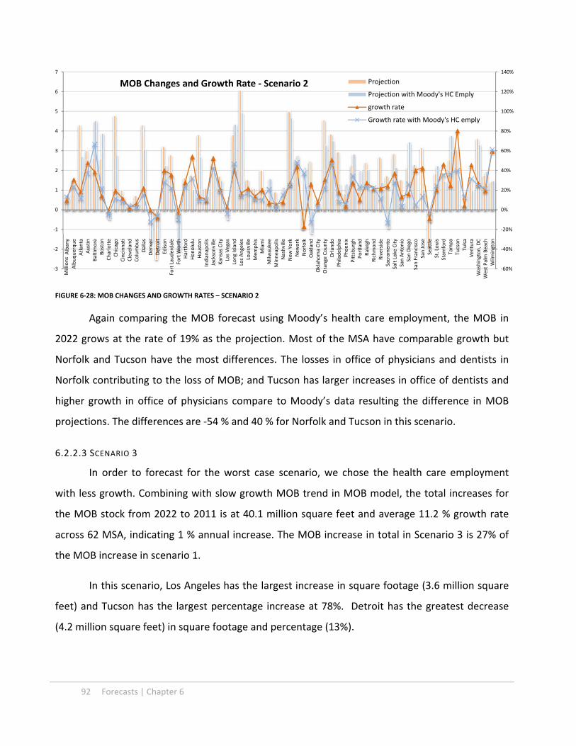
92 Forecasts | Chapter 6
FIGURE 6‐28: MOB CHANGES AND GROWTH RATES – SCENARIO 2
Again comparing the MOB forecast using Moody’s health care employment, the MOB in
2022 grows at the rate of 19% as the projection. Most of the MSA have comparable growth but
Norfolk and Tucson have the most differences. The losses in office of physicians and dentists in
Norfolk contributing to the loss of MOB; and Tucson has larger increases in office of dentists and
higher growth in office of physicians compare to Moody’s data resulting the difference in MOB
projections. The differences are ‐54 % and 40 % for Norfolk and Tucson in this scenario.
6.2.2.3 SCENARIO 3
In order to forecast for the worst case scenario, we chose the health care employment
with less growth. Combining with slow growth MOB trend in MOB model, the total increases for
the MOB stock from 2022 to 2011 is at 40.1 million square feet and average 11.2 % growth rate
across 62 MSA, indicating 1 % annual increase. The MOB increase in total in Scenario 3 is 27% of
the MOB increase in scenario 1.
In this scenario, Los Angeles has the largest increase in square footage (3.6 million square
feet) and Tucson has the largest percentage increase at 78%. Detroit has the greatest decrease
(4.2 million square feet) in square footage and percentage (13%).
‐60%
‐40%
‐20%
0%
20%
40%
60%
80%
100%
120%
140%
‐3
‐2
‐1
0
1
2
3
4
5
6
7Albany
Albuquerque
Atlanta
Austin
Baltimore
Boston
Charlotte
Chicago
Cincinnati
Cleveland
Columbus
Dallas
Den
ver
Detroit
Edison
Fort Lauderdale
Fort W
orth
Hartford
Honolulu
Houston
Indianapolis
Jacksonville
Kansas City
Las Vegas
Long Island
Los Angeles
Louisville
Mem
phis
Miami
Milw
aukee
Minneapolis
Nashville
New
York
New
ark
Norfolk
Oakland
Oklahoma City
Orange County
Orlando
Philadelphia
Phoenix
Pittsburgh
Portland
Raleigh
Richmond
Riverside
Sacram
ento
Salt Lake City
San Antonio
San Diego
San Francisco
San Jose
Seattle
St. Louis
Stam
ford
Tampa
Tucson
Tulsa
Ventura
Washington, D
CWest Palm Beach
Wilm
ington
Millions
MOB Changes and Growth Rate ‐ Scenario 2 Projection
Projection with Moody's HC Emply
growth rate
Growth rate with Moody's HC emply

Chapter 6 | Forecasts 93
FIGURE 6‐29: 2022 MOB STOCK – SCENARIO 3
The strong growth in office of physicians, office of dentists, hospital and laboratories help
with the MOB growth in Tucson. Detroit suffers the most loss due to losses in office of physicians
and hospitals.
6.3 CHAPTER SUMMARY
Population growth, share of elderly group, employment and income all play different roles
in the health care employment in different MSA, and bring drastic different regional growths in
different sectors. The health care employment continues to grow base on the projected economic
and population data, and the trend in health care employment growth will likely to continue. The
area with the large population growth, aging population, and better employment outlook
continue to demand more health care services. Health care practices also continue to shift
towards to outpatient services.
MOB is increasing due to the health care employment increases directly. With scenario 2
and 3, we can see the decreases in health care employment growth diminish the MOB growth by
more than 10%. However, the development trend also has considerable impact on how much
MOB increase. Between scenario 1 and 2 control all other factors, the trend in MOB model slows
the MOB growth by almost 6 %.
‐0.3
‐0.1
0.1
0.3
0.5
0.7
0.9
‐10
‐5
0
5
10
15
20
25
30
35
40
45Albany
Albuquerque
Atlanta
Austin
Baltimore
Boston
Charlotte
Chicago
Cincinnati
Cleveland
Columbus
Dallas
Den
ver
Detroit
Edison
Fort Lauderdale
Fort W
orth
Hartford
Honolulu
Houston
Indianapolis
Jacksonville
Kansas City
Las Vegas
Long Island
Los Angeles
Louisville
Mem
phis
Miami
Milw
aukee
Minneapolis
Nashville
New
York
New
ark
Norfolk
Oakland
Oklahoma City
Orange County
Orlando
Philadelphia
Phoenix
Pittsburgh
Portland
Raleigh
Richmond
Riverside
Sacram
ento
Salt Lake City
San Antonio
San Diego
San Francisco
San Jose
Seattle
St. Louis
Stam
ford
Tampa
Tucson
Tulsa
Ventura
Washington, D
CWest Palm Beach
Wilm
ington
Millions
2022 MOB stock‐ Scenario 3addition
Stock 2011
growth rate

94 Forecasts | Chapter 6
Regional characteristics also weigh in on the development of MOB. Region such as Norfolk
which has the most shifts on medical practice in the past has extreme outcome on the health care
employment changes when the population and employment are only less positive. It introduces
extreme lost in MOB for Norfolk in Scenario 2; whereas Detroit’s losses are due to the
fundamental loss in population and worse employment outlook. Region such as Tucson, which has
large shifts in health care practice in addition to the positive employment outlook, substantial
population growth and increase in the share of age group 65+, has the extreme growth in MOB
spaces. Areas such as Honolulu, Jacksonville and Wilmington also have larger shares of group 65+
and increases for income to demand more health care and MOB growth. Note that the small size
of MOB markets in these regions might contribute to the extreme outcomes15.
The summary of three scenarios from MOB is tabulated in the following in table. We can
see with different average growth rates, regional growths very greatly.
MOB stock 2011 Scenario 1 Scenario 2 Scenario 3
Total 690,137,899 838,069,653 808,716,725 730,265,009
Total increase 147,931,754 118,578,826 40,127,110
Average growth 28.50% 22.52% 11.20%
Max Los Angeles Los Angeles Los Angeles Los Angeles
36,517,625 43,729,752 42,594,049 40,117,312
Min Wilmington Wilmington Wilmington
2,384,653 4,270,281 3,813,624 3,515,484
Max increase Los Angeles Los Angeles Los Angeles
7,212,127 6,076,424 3,599,687
Max decrease Detroit Detroit Detroit
(2,224,645) (2,506,434) (4,153,366)
Max % increase Tucson Tucson Tucson
97.07% 80.43% 78.00%
Max % decrease Detroit Norfolk Detroit
‐6.91% ‐16.85% ‐12.90% TABLE 6‐1: MOB STOCK
Three scenarios for MOB in 2022 populated in Figure 6‐30 and 6‐31 depict the ranges of
differences in growth and MOB stock across 62 MSAs. Between scenario 1 and scenario 2 with the
difference in MOB trend, the results are fairly similar but scenario 2 has slightly less values across
15 See Figure 6‐26

Chapter 6 | Forecasts 95
MSAs with couple exceptions. Here are the greatest differences between these two scenarios
among MSAs: In square footage term, Seattle has 1.39 million square feet less million square feet,
losing 1.83 million square feet in total in Scenario 2; and Chicago has 0.53 million square feet more,
adding total of 4.79 million square feet in MOB development in Scenario 2. In percentage term,
Wilmington has 19% less growth, and its growth rate drop to 59.9%; and Chicago has more 2.3% in
growth, and its growth rate reaches 19.7% in Scenario 2.
Between the Scenario 2 and 3, greater differences in forecasts express the greater
influences of health care employment growth and shifts on MOB market. Dallas has lost 4.5
million square feet in MOB increases in Scenario 3. Dallas’ MOB increases change from 4.3 million
square feet increase to 2.4 million decreases. Norfolk has 0.89 million square feet less in the loss
of MOB. The loss changes from 0.98 million to 0.09 million square feet between the Scenario 2
and 3; Edison has the greatest loss in growth percentage at 31.3%, and the growth rate dropped to
8.9% in Scenario 3; whereas Norfolk has 15.3 % less loss in growth, and reaches 1.6% loss in
growth rate in Scenario 3.
3 scenarios created by changes in MOB trend and health care employment trend have
different reactions across MSAs. Also notice that the MSA with highest populations do not equate
to the largest MOB markets. This also demonstrates the regional characteristics have great
influences on MOB markets.

96 Forecasts | Chapter 6
FIGURE 6‐30: MOB GROWTH RATES – 3 SCENARIOS
FIGURE 6‐31: MOB IN 2022 – 3 SCENARIOS16
16 See Appendix L4 for the full data
‐40%
‐20%
0%
20%
40%
60%
80%
100%Albany
Albuquerque
Atlanta
Austin
Baltimore
Boston
Charlotte
Chicago
Cincinnati
Cleveland
Columbus
Dallas
Den
ver
Detroit
Edison
Fort Lauderdale
Fort W
orth
Hartford
Honolulu
Houston
Indianapolis
Jacksonville
Kansas City
Las Vegas
Long Island
Los Angeles
Louisville
Mem
phis
Miami
Milw
aukee
Minneapolis
Nashville
New
York
New
ark
Norfolk
Oakland
Oklahoma City
Orange County
Orlando
Philadelphia
Phoenix
Pittsburgh
Portland
Raleigh
Richmond
Riverside
Sacram
ento
Salt Lake City
San Antonio
San Diego
San Francisco
San Jose
Seattle
St. Louis
Stam
ford
Tampa
Tucson
Tulsa
Ventura
Washington, D
CWest Palm Beach
Wilm
ington
MOB Growth Rate
Scenario 1 Scenario 2 Scenario 3
‐20%
0%
20%
40%
60%
80%
100%
‐10
0
10
20
30
40
50
Albany
Albuquerque
Atlanta
Austin
Baltimore
Boston
Charlotte
Chicago
Cincinnati
Cleveland
Columbus
Dallas
Denver
Detroit
Edison
Fort Lauderdale
Fort W
orth
Hartford
Honolulu
Houston
Indianapolis
Jacksonville
Kansas City
Las Vegas
Long Island
Los Angeles
Louisville
Memphis
Miami
Milw
aukee
Minneapolis
Nashville
New York
Newark
Norfolk
Oakland
Oklahoma City
Orange County
Orlando
Philadelphia
Phoen
ix
Pittsburgh
Portland
Raleigh
Richmond
Riverside
Sacram
ento
Salt Lake City
San Antonio
San Diego
San Francisco
San Jose
Seattle
St. Louis
Stam
ford
Tampa
Tucson
Tulsa
Ven
tura
Washington, D
C
West Palm Beach
Wilm
ington
Millions
MOB in 2002 ‐ 3 Scenarios
Scenario 1 Scenario 2 Scenario 3 Average growth rate

Chapter 7 | Conclusion 97
Chapter 7. CONCLUSION Our attempt to look into the future medical office building development concerning
upcoming population, economic and political changes in the US presented in this paper is to
utilize a system built from the analysis of the available data and the applicable real estate
research methodology. This system quantifies the dynamic relationships among factors, and
allows us to forecast the MOB market in 2022. We have concluded that medical office building
market will increase on average even under the unfavorable condition. However, substantial
differences in growth among regions are also in the finding, and they can be explained
systematically.
Demographic changes, economic factors, health care practice trend, and real estate
trend as market forces for medical office buildings intricately influent one another. After
developing the basic system that incorporates all forces, and with the projected data from
Moody’s, we believe that the market of medical office buildings will be expanding greatly.
The health care employment growth can explain the growth in medical office buildings
partially. The demographic shift, economic condition and locality have driven the growth in
health care employment. Understandably, the growing population has the biggest impact on
health care employment as it is the most fundamental demand driver for the medical service
market. However, different medical services respond to different demand drivers differently.
For example, office of physicians and medical and diagnostic are sensitive to changes of
employment, and office of dentists and medical and surgical hospitals are affected more by
changes of the share of elderly group additionally. The locality also plays an important role in
health care employment. The area such as Tucson projected to have strong employment and
population growth, combining with the large increase in share of elderly and the greater shift in
health care practice, Tucson is positioned to enjoy strong growth in health care employment.
How different sectors in health care growth also contributes differently to medical office
buildings grow. The strongest demand per employment for medical office building falls on
dentists’ offices, however, greater numbers of employment for physicians’ offices and hospitals
98 Conclusion | Chapter 7
demand more medical office spaces in aggregates. The area such as Honolulu has strong
demand for medical office buildings because of the increase in offices of physicians. Tucson’s
considerable increase in hospital employment, in additional to its growth in total health care
employment, also pushes the growth in medical office buildings higher.
Commercial influences such as capital market and development mechanism also have
their presences in the medical office building market, as it is still belong to the broader real
estate market. More investment activities are involved with the health care real estate in the
recent years due to more liquidity, more stable tenants and strong medical service demand.
Many expect the market for medical office building will continue to grow because of the
upcoming outpatient service demand. Discussions such as hospitals using medical office
buildings as strategies to manage costs, retain talents and improve balances sheets are also
explicit. These influences of market expectation and development preferences represented by
trends in the models predict how much medical office building will grow in addition to the
growth generated by health care practices.
We develop three scenarios for forecasts of future MOB across 62 MSAs, and these
scenarios cast a range of conditions from the continuous growth in both health care and real
estate as Scenario 1, continuous growth in the health care but slow‐down in the real estate as
Scenario 2, and to the slow‐down in both markets as Scenario 3. The following Figures
demonstrate the performances of each market by ranks as shown in Figure 7‐1. Each market
has different reasons for strong growth or loss but in aggregates, these are the best market and
the worst markets in the next 10 years: the strongest markets for growth across three scenarios
are Tucson, Wilmington, Honolulu and Jacksonville. The consistently weak markets in growth
rates are Detroit, Fort Worth, Charlotte and Seattle.
The markets with largest square footage increases and decreases across are Los Angeles
and Detroit as shown in Figure 7‐2; MOB markets in areas such as New York and Orange county
with large square footage increases in scenario 1 and 2, but have less in scenario 3, have
stronger dependency on health care employment; whereas Washington DC area is less
influenced by in the health care growth, and it reflects on the less square footage difference
Chapter 7 | Conclusion 99
between scenario 2 and scenario 3. Beside Detroit, both Fort Worth and Seattle have square
footage decrease in all scenarios. Norfolk has strong health care shift have less loss when the
shift was stalled by the slowing down of health care employment, resulting less loss in square
footage in MOB in scenario 3.
These significant differences across regions prove that MOB market is highly dependent
on local conditions. These local conditions could be the local economic reality, different
population growth pattern, health care development or the real estate development. Although
the MOB market in the US in general is positive, local MOB markets are telling each of its own
stories.
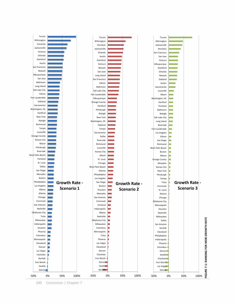
100 Conclusion | Chapter 7
‐50% 0% 50% 100%
Detroit
Seattle
Fort Worth
Norfolk
Charlotte
Las Vegas
Denver
Cleveland
Minneapolis
Columbus
Phoenix
Houston
Indianapolis
Milwaukee
Tulsa
Oklahoma City
Nashville
San Antonio
Cincinnati
Chicago
Atlanta
Albany
Los Angeles
Philadelphia
Boston
Memphis
San Diego
Dallas
St. Louis
Portland
West Palm Beach
Riverside
Pittsburgh
Miami
Kansas City
Orange County
Louisville
Tampa
Richmond
Raleigh
New York
Hartford
Washington, DC
Sacramento
Oakland
Fort Lauderdale
Edison
Salt Lake City
Long Island
Baltimore
San Jose
Albuquerque
Newark
San Francisco
Austin
Stamford
Orlando
Ventura
Jacksonville
Honolulu
Wilmington
Tucson
Growth Rate ‐Scenario 1
‐50% 0% 50% 100%
Norfolk
Seattle
Detroit
Fort Worth
Charlotte
Denver
Cleveland
Las Vegas
Phoenix
Tulsa
Minneapolis
Columbus
Milwaukee
Oklahoma City
Nashville
Albany
Indianapolis
Portland
Cincinnati
San Antonio
Memphis
Houston
Boston
San Diego
Los Angeles
Philadelphia
Atlanta
West Palm Beach
Chicago
St. Louis
Miami
Kansas City
Louisville
Richmond
Riverside
Dallas
Sacramento
Tampa
Oakland
Washington, DC
New York
Raleigh
Pittsburgh
Hartford
Orange County
Albuquerque
Fort Lauderdale
Salt Lake City
Baltimore
Edison
San Francisco
Long Island
San Jose
Newark
Ventura
Stamford
Austin
Orlando
Jacksonville
Honolulu
Wilmington
Tucson
Growth Rate ‐Scenario 2
‐50% 0% 50% 100%
Detroit
Las Vegas
Fort Worth
Charlotte
Seattle
Denver
Columbus
Phoenix
Indianapolis
Philadelphia
Cleveland
Norfolk
San Antonio
Dallas
Milwaukee
Nashville
Houston
Minneapolis
Oklahoma City
Chicago
Atlanta
St. Louis
Cincinnati
Tulsa
Tampa
Pittsburgh
New York
Kansas City
Memphis
Orange County
Albany
Boston
West Palm Beach
Richmond
San Diego
Edison
Los Angeles
Fort Lauderdale
Riverside
Long Island
Salt Lake City
Raleigh
Baltimore
Portland
Hartford
Washington, DC
Miami
Louisville
Sacramento
Austin
Oakland
Newark
Orlando
Stamford
Albuquerque
Ventura
San Jose
San Francisco
Honolulu
Jacksonville
Wilmington
Tucson
Growth Rate ‐Scenario 3
FIGURE 7‐1: RANKING FOR M
OB GROWTH
RATE

Chapter 7 | Conclusion 101
‐5 0 5 10
Detroit
Seattle
Fort Worth
Norfolk
Charlotte
Cleveland
Las Vegas
Tulsa
Denver
Albany
Milwaukee
Columbus
Oklahoma City
Nashville
Minneapolis
Cincinnati
Richmond
Indianapolis
Memphis
Ventura
San Antonio
Wilmington
Hartford
Portland
Phoenix
St. Louis
Louisville
West Palm Beach
Stamford
Honolulu
Pittsburgh
Albuquerque
Kansas City
Sacramento
San Diego
Raleigh
Newark
Miami
Baltimore
San Francisco
Jacksonville
Fort Lauderdale
Tampa
Salt Lake City
Riverside
Edison
Philadelphia
Austin
Oakland
San Jose
Houston
Tucson
Boston
Long Island
Dallas
Orlando
Chicago
Atlanta
Orange County
Washington, DC
New York
Los Angeles
Difference in MOB
‐Scenario 1
‐5 0 5 10
Detroit
Seattle
Norfolk
Fort Worth
Charlotte
Denver
Cleveland
Tulsa
Las Vegas
Albany
Milwaukee
Oklahoma City
Nashville
Columbus
Phoenix
Portland
Minneapolis
Cincinnati
Richmond
Indianapolis
Memphis
Wilmington
Ventura
Albuquerque
San Antonio
Louisville
Hartford
Kansas City
Sacramento
West Palm Beach
Honolulu
St. Louis
Stamford
Miami
San Diego
Pittsburgh
San Francisco
Jacksonville
Raleigh
Oakland
Newark
Tampa
Boston
Baltimore
Riverside
Fort Lauderdale
Salt Lake City
Philadelphia
Austin
Tucson
San Jose
Edison
Washington, DC
Long Island
Houston
Orlando
Atlanta
Dallas
Orange County
Chicago
New York
Los Angeles
Millions
Difference in MOB
‐Scenario 2
‐5 0 5
Detroit
Fort Worth
Seattle
Las Vegas
Denver
Phoenix
Charlotte
Columbus
Philadelphia
Dallas
Indianapolis
Cleveland
San Antonio
Houston
Norfolk
Minneapolis
Milwaukee
Nashville
Oklahoma City
St. Louis
Cincinnati
Tulsa
Pittsburgh
Richmond
Albany
Tampa
Chicago
Kansas City
Memphis
Atlanta
Edison
West Palm Beach
Hartford
Fort Lauderdale
Ventura
Baltimore
New York
Orange County
Salt Lake City
Wilmington
San Diego
Stamford
Louisville
Long Island
Raleigh
Portland
Honolulu
Austin
Boston
Albuquerque
Miami
Riverside
Newark
Sacramento
San Francisco
Jacksonville
Washington, DC
Orlando
San Jose
Oakland
Tucson
Los Angeles
Difference in MOB
‐Scenario 3
FIGURE 7‐2 : RANKING FOR M
OB SQUARE FO
OTA
GE INCREA
SE

102 Conclusion | Chapter 7
(This page is intentionally blank)

| Bibliography 103
BIBLIOGRAPHY American Hospital Association “The migration of Care to Non‐hospital Settings: Have regulatory Structures Kept
Pace with Changes in Care Delivery?” Trendwatch, (July, 2006) Beatty, Paul C. Ph.D., Hsiao, Chun‐Ju. Ph.D., Cherry, Donald. M.S., Rechtsteiner. M.S. “National Ambulatory Medical
Care Survey: 2007 Summary.” National Health statistics Reports, (November 3, 2010) Bernstein, Daniel and Doctrow, Jerry. “Healthcare REITS: Antidote For an Economic Downturn?” Stifel Nicolaus
Equity Research Industry Analysis (Winter 2008) Bronner, Kristen K. M.A., Fisher, Elliott S. M.D., Ph.D., Goodman, David C. “Hospital and Physician Capacity Update.”
A Dartmouth Atlas Project Brief Report, (March 30, 2009) Burns, Lawton Robert., Muller, Ralph W. “Hospital‐Physician Collaboration: Landscape of Economic Integration and
Impact on Clinical Integration.” The Milbank Quarterly, Vol. 86, No. 3 (2008) Cain Brothers, “Physician Ownership Participation in Medical Office Buildings,” Strategies in Capital Finance,
Volume 51 (July 2006) Cain Brothers. “From Strategic Assets to Tactical Investments: Changing Attitudes Toward Medical Office Building
Ownership.” Strategies in Capital Finance, Vol. 41 (Summer 2003) Cain Brothers. “Medical Real Estate: Trend in Third Party Development—From Niche to Mainstream” Strategies in
Capital Finance, Vol. 46 (July 2005) Cassidy Turley. “Insights: How will Healthcare Reform Impact commercial Real Estate?” cassidyturley.com. 2010.
www.cassidyturley.com Cherry, Donald. M.S., Lucas, Christine. M.P.H., M.S.W., Decker, Sandra L. Ph.D. “Population Aging and the Use of
Office‐based Physician Services.” NCHS Data Brief, No. 41 (August 2010) Cutler, David M., Meara, Ellen and White, Chapin. “Trends in Medical Spending By Age, 1963‐2000.” Health Affairs,
Volume 23, No. 4 ( July/August, 2004) Shilling, Gary. “The Outlook for Health Care.” Urban Land Institute, (2011)

104 Bibliography |
(This page is intentionally blank)

Appendix D | Appendix A 105
APPENDIX A
National Health Expenditure Projections 2009‐2019
Prior Law baseline 2010 2011 2012 2013 2014 2015 2016 2017 2018 2019
Total, CY
2010‐2019
Health Expenditures
(NHE) $2,632.2 $2,778.7 $2,944.4 $3,125.4 $3,325.5 $3,551.5 $3,798.5 $4,067.7 $4,358.8 $4,670.6 $35,253.3
Medicare $515.5 $550.5 $591.0 $634.1 $679.7 $732.1 $790.4 $857.2 $930.9 $1,010.9 $7,292.3
Medicaid/CHIP $436.1 $473.0 $512.4 $553.4 $593.9 $641.7 $696.6 $755.9 $821.7 $893.2 $6,377.9
Federal $282.2 $277.9 $292.7 $315.9 $337.8 $364.3 $395.0 $427.9 $464.6 $504.5 $3,662.8
State & Local $153.9 $195.1 $219.6 $237.6 $256.1 $277.4 $301.5 $328.0 $357.1 $388.7 $2,715.1
Other Public $307.7 $325.1 $343.9 $364.6 $386.6 $410.5 $436.4 $464.0 $493.2 $523.6 $4,055.5
Out of Pocket $285.1 $297.7 $308.9 $322.3 $340.3 $359.4 $379.1 $400.2 $422.8 $446.7 $3,562.4
Sponsored Private
Health Insurance $847.0 $879.0 $919.3 $966.0 $1,024.5 $1,088.4 $1,156.0 $1,228.7 $1,305.6 $1,387.3 $10,801.8
Other Private Health
Insurance* $49.2 $51.0 $54.6 $57.7 $59.4 $61.5 $63.5 $65.9 $68.2 $70.6 $601.7
Other Private† $191.6 $202.4 $214.5 $227.3 $241.1 $257.8 $276.4 $296.0 $316.4 $338.3 $2,561.8
Gross Domestic
Product (GDP)‡ 17.8% 17.9% 18.1% 18.3% 18.6% 19.0% 19.4% 19.8% 20.3% 20.8%
New Law PPACA 2010 2011 2012 2013 2014 2015 2016 2017 2018 2019
Total, CY
2010‐2019
Health Expenditures
(NHE) 2,636.4 2,774.4 2,932.7 3,101.5 3,358.8 3,615.9 3,875.2 4,139.6 4,413.1 4,716.5 35,564.0
Medicare 516.0 545.7 577.1 604.8 626.1 682.1 726.1 778.1 836.4 897.9 6,790.2
Medicaid/CHIP 434.2 471.4 513.3 557.7 657.3 716.6 779.4 832.7 900.8 977.9 6,841.4
Federal 281.2 277.4 294.5 321.4 398.3 435.7 478.2 503.6 543.8 588.7 4,122.7
State & Local 153.0 194.1 218.9 236.3 259.0 280.8 301.2 329.1 357.1 389.2 2,718.7
Other Public 312.3 325.2 344.0 364.9 381.7 406.2 434.6 463.4 493.5 523.6 4,049.4
Out of Pocket 285.1 297.9 308.6 321.6 313.6 323.9 334.7 352.5 381.4 405.8 3,325.1
Sponsored Private
Health Insurance 848.2 881.0 921.3 968.3 1,038.8 1,112.3 1,160.7 1,212.2 1,259.7 1,336.1 10,738.7
Other Private Health
Insurance* 49.3 50.9 54.1 57.0 14.9 14.9 14.5 14.2 13.9 13.6 297.4
Other Private† 191.4 202.3 214.3 227.2 234.8 251.9 272.8 293.4 314.5 335.6 2,538.1
Exchange — — — — 91.7 107.9 152.4 193.1 212.8 225.8 983.7
Gross Domestic
Product (GDP)‡ 17.8% 17.9% 18.0% 18.2% 18.8% 19.3% 19.8% 20.2% 20.5% 21.0%
22‐Apr‐10
*In the prior‐law baseline, other private health insurance includes private Medicare supplemental coverage and individual coverage. In the new‐law
estimates, other private health insurance includes only those with Medicare supplemental coverage.†In the NHE accounts, other private spending includes philanthropic giving and income from non‐pa ent sources, such as parking and investment income,
for institutional providers.‡Based on Gross Domes c Product (GDP) projec ons that accompanied the February 24, 2009 NHE projec ons release for 2008‐2018.
(http://www.cms.hhs.gov/NationalHealthExpendData/downloads/proj2008.pdf )
Source: Centers for Medicare & Medicaid Services, Office of the Actuary.
Table 5 — Estimated Increases (+) or Decreases (–) in National Health Expenditures under the Patient Protection and Affordable Care Act, as Enacted and
Amended, in bil l ions
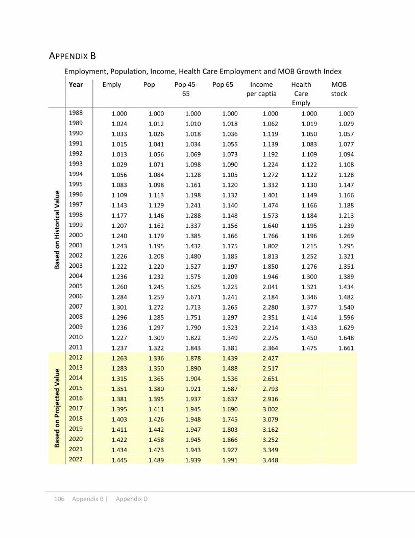
106 Appendix B | Appendix D
APPENDIX B
Employment, Population, Income, Health Care Employment and MOB Growth Index
Year Emply Pop Pop 45‐65
Pop 65 Income per captia
Health Care Emply
MOB stock
Based on Historical V
alue
1988 1.000 1.000 1.000 1.000 1.000 1.000 1.000
1989 1.024 1.012 1.010 1.018 1.062 1.019 1.029
1990 1.033 1.026 1.018 1.036 1.119 1.050 1.057
1991 1.015 1.041 1.034 1.055 1.139 1.083 1.077
1992 1.013 1.056 1.069 1.073 1.192 1.109 1.094
1993 1.029 1.071 1.098 1.090 1.224 1.122 1.108
1994 1.056 1.084 1.128 1.105 1.272 1.122 1.128
1995 1.083 1.098 1.161 1.120 1.332 1.130 1.147
1996 1.109 1.113 1.198 1.132 1.401 1.149 1.166
1997 1.143 1.129 1.241 1.140 1.474 1.166 1.188
1998 1.177 1.146 1.288 1.148 1.573 1.184 1.213
1999 1.207 1.162 1.337 1.156 1.640 1.195 1.239
2000 1.240 1.179 1.385 1.166 1.766 1.196 1.269
2001 1.243 1.195 1.432 1.175 1.802 1.215 1.295
2002 1.226 1.208 1.480 1.185 1.813 1.252 1.321
2003 1.222 1.220 1.527 1.197 1.850 1.276 1.351
2004 1.236 1.232 1.575 1.209 1.946 1.300 1.389
2005 1.260 1.245 1.625 1.225 2.041 1.321 1.434
2006 1.284 1.259 1.671 1.241 2.184 1.346 1.482
2007 1.301 1.272 1.713 1.265 2.280 1.377 1.540
2008 1.296 1.285 1.751 1.297 2.351 1.414 1.596
2009 1.236 1.297 1.790 1.323 2.214 1.433 1.629
2010 1.227 1.309 1.822 1.349 2.275 1.450 1.648
2011 1.237 1.322 1.843 1.381 2.364 1.475 1.661
Based on Projected Value
2012 1.263 1.336 1.878 1.439 2.427
2013 1.283 1.350 1.890 1.488 2.517
2014 1.315 1.365 1.904 1.536 2.651
2015 1.351 1.380 1.921 1.587 2.793
2016 1.381 1.395 1.937 1.637 2.916
2017 1.395 1.411 1.945 1.690 3.002
2018 1.403 1.426 1.948 1.745 3.079
2019 1.411 1.442 1.947 1.803 3.162
2020 1.422 1.458 1.945 1.866 3.252
2021 1.434 1.473 1.943 1.927 3.349
2022 1.445 1.489 1.939 1.991 3.448

Appendix D | Appendix C 107
APPENDIX C
Population for Total 62 MSAs
Year Total Population
Population 45‐65
Population 65+
Share of 45‐65
Share of 65+
Share of 45+
Historical V
alue
1988 130178 24045 14945 18.5% 11.5% 30.0%
1989 131773 24279 15212 18.4% 11.5% 30.0%
1990 133580 24487 15489 18.3% 11.6% 29.9%
1991 135517 24865 15766 18.3% 11.6% 30.0%
1992 137500 25712 16032 18.7% 11.7% 30.4%
1993 139359 26400 16295 18.9% 11.7% 30.6%
1994 141158 27133 16512 19.2% 11.7% 30.9%
1995 142981 27911 16731 19.5% 11.7% 31.2%
1996 144923 28795 16916 19.9% 11.7% 31.5%
1997 147013 29846 17044 20.3% 11.6% 31.9%
1998 149158 30964 17155 20.8% 11.5% 32.3%
1999 151319 32145 17273 21.2% 11.4% 32.7%
2000 153476 33309 17429 21.7% 11.4% 33.1%
2001 155534 34438 17564 22.1% 11.3% 33.4%
2002 157257 35597 17708 22.6% 11.3% 33.9%
2003 158822 36724 17887 23.1% 11.3% 34.4%
2004 160428 37863 18070 23.6% 11.3% 34.9%
2005 162136 39062 18306 24.1% 11.3% 35.4%
2006 163864 40180 18545 24.5% 11.3% 35.8%
2007 165536 41191 18906 24.9% 11.4% 36.3%
2008 167228 42100 19379 25.2% 11.6% 36.8%
2009 168848 43043 19771 25.5% 11.7% 37.2%
2010 170420 43805 20154 25.7% 11.8% 37.5%
2011 172087 44324 20643 25.8% 12.0% 37.8%
Projected Value
2012 173901 45161 21509 26.0% 12.4% 38.3%
2013 175768 45435 22236 25.8% 12.7% 38.5%
2014 177679 45789 22956 25.8% 12.9% 38.7%
2015 179624 46201 23712 25.7% 13.2% 38.9%
2016 181623 46565 24461 25.6% 13.5% 39.1%
2017 183640 46764 25250 25.5% 13.7% 39.2%
2018 185665 46830 26078 25.2% 14.0% 39.3%
2019 187700 46817 26951 24.9% 14.4% 39.3%
2020 189759 46777 27883 24.7% 14.7% 39.3%
2021 191807 46713 28801 24.4% 15.0% 39.4%
2022 193850 46634 29751 24.1% 15.3% 39.4% Data Source: CBRE, Moody’s Corp

108 Appendix D | Appendix D
APPENDIX D
Population Changes
Changes from 1988‐2011 Percentage Changes from 1988‐2011
MSA Total Pop.
Pop. 45‐65
Pop. 65+ Pop.
Employ per captia
Income per captia
45‐65 group share change
65+ group share change
Albany 74.42 101.45 16.60 9.3% 0.95% 135.9% 10.0% 0.7%
Albuquerque 314.83 139.45 56.13 53.8% ‐7.51% 131.7% 9.4% 2.7%
Atlanta 2383.23 836.69 249.25 80.5% ‐17.95% 116.3% 7.9% 1.0%
Austin 965.09 290.17 84.10 117.8% ‐0.90% 137.9% 8.4% 0.5%
Baltimore 388.07 307.77 82.36 16.6% ‐1.08% 161.7% 8.5% 1.4%
Boston 632.27 669.91 122.32 12.3% ‐7.18% 153.7% 9.6% 0.8%
Charlotte 812.28 264.05 83.55 82.0% ‐14.13% 129.8% 6.2% 0.0%
Chicago 1328.65 878.77 174.14 17.7% ‐4.99% 132.4% 7.2% 0.3%
Cincinnati 322.28 246.99 54.09 17.7% 1.74% 133.1% 8.7% 0.8%
Cleveland ‐33.89 174.72 29.98 ‐1.6% 0.83% 124.3% 8.8% 1.7%
Columbus 480.88 228.71 63.86 34.9% ‐1.52% 127.4% 7.7% 0.9%
Dallas 1815.99 616.40 180.92 71.4% ‐12.02% 126.4% 7.3% 0.9%
Denver 1043.44 434.93 137.23 56.1% ‐5.01% 159.8% 8.7% 1.6%
Detroit 69.74 421.47 93.91 1.6% ‐5.85% 117.0% 9.2% 1.9%
Edison 488.10 288.89 91.77 26.1% ‐3.07% 142.0% 8.1% 1.0%
Fort Lauderdale 553.00 263.09 4.08 45.6% 0.29% 107.0% 9.0% ‐6.3%
Fort Worth 869.43 317.03 96.58 65.5% ‐3.47% 135.8% 7.7% 1.0%
Hartford 94.86 130.45 31.90 8.5% ‐12.99% 136.5% 9.2% 1.6%
Honolulu 137.44 99.70 59.45 16.7% ‐0.61% 138.2% 7.8% 4.7%
Houston 2479.94 885.80 278.60 68.2% ‐3.45% 182.7% 7.7% 1.7%
Indianapolis 518.08 235.76 59.90 37.0% ‐0.38% 122.4% 7.2% 0.1%
Jacksonville 464.63 213.59 72.69 51.8% ‐2.97% 139.8% 9.5% 1.7%
Kansas City 447.91 246.98 62.07 27.7% ‐4.15% 138.6% 7.9% 0.5%
Las Vegas 1322.30 361.03 162.22 202.7% ‐13.30% 111.8% 4.9% 1.4%
Long Island 231.87 252.22 103.19 8.8% 0.10% 127.9% 7.1% 2.6%
Los Angeles 1265.68 956.96 257.00 14.6% ‐17.86% 127.1% 7.5% 1.3%
Louisville 246.14 158.95 40.81 23.4% 0.31% 135.2% 8.6% 0.8%
Memphis 277.12 162.79 34.90 26.3% 1.30% 148.7% 8.6% 0.5%
Miami 648.29 268.09 98.45 34.6% ‐7.09% 136.6% 5.4% 0.3%
Milwaukee 150.82 160.71 25.56 10.7% 1.78% 143.5% 8.5% 0.4%
Minneapolis 852.23 475.18 115.90 34.5% ‐3.85% 142.1% 10.0% 1.0%
Nashville 597.27 232.90 66.15 58.0% ‐7.53% 138.9% 7.5% 0.1%
New York 1229.56 865.68 127.83 11.8% ‐8.08% 149.5% 5.3% ‐0.3%
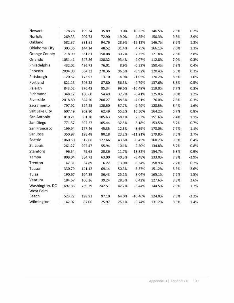
Appendix D | Appendix D 109
Newark 178.78 199.24 35.89 9.0% ‐10.52% 146.5% 7.5% 0.7%
Norfolk 269.33 209.73 72.90 19.0% 4.85% 150.3% 9.8% 2.9%
Oakland 582.37 331.51 94.76 28.9% ‐12.12% 146.7% 8.6% 1.3%
Oklahoma City 303.36 144.14 48.52 31.4% 4.75% 166.1% 7.0% 1.3%
Orange County 718.99 361.61 150.08 30.7% ‐7.35% 121.8% 7.6% 2.8%
Orlando 1051.41 347.86 128.32 93.4% ‐4.07% 112.8% 7.0% ‐0.3%
Philadelphia 432.02 496.73 76.01 8.9% ‐0.53% 150.4% 7.8% 0.4%
Phoenix 2094.08 634.32 270.36 96.5% ‐9.92% 120.4% 6.3% 0.3%
Pittsburgh ‐120.52 173.97 3.10 ‐4.9% 21.05% 170.2% 8.5% 1.0%
Portland 821.13 346.38 87.80 56.3% ‐4.79% 137.6% 8.8% ‐0.5%
Raleigh 843.52 276.43 85.34 99.6% ‐16.48% 119.0% 7.7% 0.3%
Richmond 348.12 180.60 54.49 37.7% ‐6.41% 125.0% 9.0% 1.2%
Riverside 2018.80 644.50 208.27 88.3% ‐4.01% 76.0% 7.6% ‐0.3%
Sacramento 797.92 324.25 120.50 57.7% ‐9.49% 128.5% 8.4% 1.6%
Salt Lake City 607.49 202.80 62.49 55.2% 16.50% 164.2% 6.7% 0.8%
San Antonio 810.21 301.20 105.63 58.1% 2.53% 151.6% 7.4% 1.1%
San Diego 771.57 397.27 105.44 32.5% 3.18% 153.5% 8.7% 0.7%
San Francisco 199.94 177.46 45.35 12.5% ‐8.69% 178.0% 7.7% 1.1%
San Jose 350.97 198.48 80.18 23.2% ‐11.21% 179.8% 7.3% 2.7%
Seattle 1060.50 512.06 127.66 43.6% ‐0.45% 168.2% 9.3% 0.4%
St. Louis 261.27 297.47 55.94 10.1% 2.50% 134.8% 8.7% 0.8%
Stamford 96.54 79.65 20.36 11.7% ‐13.82% 154.7% 6.3% 0.9%
Tampa 809.04 384.72 63.90 40.3% ‐3.48% 133.0% 7.9% ‐3.9%
Trenton 42.31 34.89 6.22 13.0% 8.34% 158.9% 7.2% 0.2%
Tucson 330.79 141.12 69.14 50.3% ‐5.37% 151.2% 8.3% 2.6%
Tulsa 190.67 104.39 36.43 25.1% 8.04% 165.1% 7.2% 1.5%
Ventura 184.67 106.26 39.24 28.3% 0.42% 127.6% 8.8% 2.6%
Washington, DC 1697.86 769.29 242.51 42.2% ‐3.44% 144.5% 7.9% 1.7%
West Palm Beach 523.72 198.92 97.10 64.0% ‐10.46% 124.0% 7.3% ‐2.2%
Wilmington 142.02 87.06 25.97 25.1% ‐5.74% 131.2% 8.5% 1.4%
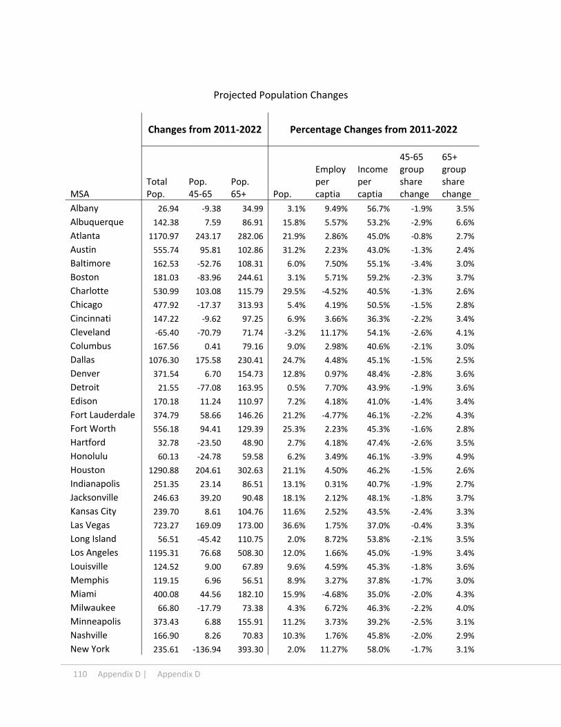
110 Appendix D | Appendix D
Projected Population Changes
Changes from 2011‐2022 Percentage Changes from 2011‐2022
MSA Total Pop.
Pop. 45‐65
Pop. 65+ Pop.
Employ per captia
Income per captia
45‐65 group share change
65+ group share change
Albany 26.94 ‐9.38 34.99 3.1% 9.49% 56.7% ‐1.9% 3.5%
Albuquerque 142.38 7.59 86.91 15.8% 5.57% 53.2% ‐2.9% 6.6%
Atlanta 1170.97 243.17 282.06 21.9% 2.86% 45.0% ‐0.8% 2.7%
Austin 555.74 95.81 102.86 31.2% 2.23% 43.0% ‐1.3% 2.4%
Baltimore 162.53 ‐52.76 108.31 6.0% 7.50% 55.1% ‐3.4% 3.0%
Boston 181.03 ‐83.96 244.61 3.1% 5.71% 59.2% ‐2.3% 3.7%
Charlotte 530.99 103.08 115.79 29.5% ‐4.52% 40.5% ‐1.3% 2.6%
Chicago 477.92 ‐17.37 313.93 5.4% 4.19% 50.5% ‐1.5% 2.8%
Cincinnati 147.22 ‐9.62 97.25 6.9% 3.66% 36.3% ‐2.2% 3.4%
Cleveland ‐65.40 ‐70.79 71.74 ‐3.2% 11.17% 54.1% ‐2.6% 4.1%
Columbus 167.56 0.41 79.16 9.0% 2.98% 40.6% ‐2.1% 3.0%
Dallas 1076.30 175.58 230.41 24.7% 4.48% 45.1% ‐1.5% 2.5%
Denver 371.54 6.70 154.73 12.8% 0.97% 48.4% ‐2.8% 3.6%
Detroit 21.55 ‐77.08 163.95 0.5% 7.70% 43.9% ‐1.9% 3.6%
Edison 170.18 11.24 110.97 7.2% 4.18% 41.0% ‐1.4% 3.4%
Fort Lauderdale 374.79 58.66 146.26 21.2% ‐4.77% 46.1% ‐2.2% 4.3%
Fort Worth 556.18 94.41 129.39 25.3% 2.23% 45.3% ‐1.6% 2.8%
Hartford 32.78 ‐23.50 48.90 2.7% 4.18% 47.4% ‐2.6% 3.5%
Honolulu 60.13 ‐24.78 59.58 6.2% 3.49% 46.1% ‐3.9% 4.9%
Houston 1290.88 204.61 302.63 21.1% 4.50% 46.2% ‐1.5% 2.6%
Indianapolis 251.35 23.14 86.51 13.1% 0.31% 40.7% ‐1.9% 2.7%
Jacksonville 246.63 39.20 90.48 18.1% 2.12% 48.1% ‐1.8% 3.7%
Kansas City 239.70 8.61 104.76 11.6% 2.52% 43.5% ‐2.4% 3.3%
Las Vegas 723.27 169.09 173.00 36.6% 1.75% 37.0% ‐0.4% 3.3%
Long Island 56.51 ‐45.42 110.75 2.0% 8.72% 53.8% ‐2.1% 3.5%
Los Angeles 1195.31 76.68 508.30 12.0% 1.66% 45.0% ‐1.9% 3.4%
Louisville 124.52 9.00 67.89 9.6% 4.59% 45.3% ‐1.8% 3.6%
Memphis 119.15 6.96 56.51 8.9% 3.27% 37.8% ‐1.7% 3.0%
Miami 400.08 44.56 182.10 15.9% ‐4.68% 35.0% ‐2.0% 4.3%
Milwaukee 66.80 ‐17.79 73.38 4.3% 6.72% 46.3% ‐2.2% 4.0%
Minneapolis 373.43 6.88 155.91 11.2% 3.73% 39.2% ‐2.5% 3.1%
Nashville 166.90 8.26 70.83 10.3% 1.76% 45.8% ‐2.0% 2.9%
New York 235.61 ‐136.94 393.30 2.0% 11.27% 58.0% ‐1.7% 3.1%

Appendix D | 111
Newark 71.19 ‐11.14 75.81 3.3% 8.48% 50.5% ‐1.4% 3.0%
Norfolk 134.19 ‐12.94 80.88 8.0% 3.03% 45.9% ‐2.6% 3.6%
Oakland 342.56 29.82 145.53 13.2% 0.25% 38.4% ‐2.1% 3.6%
Oklahoma City 158.13 7.86 61.53 12.4% 5.15% 58.8% ‐2.2% 3.0%
Orange County 371.46 24.10 166.91 12.1% 2.04% 49.3% ‐2.1% 3.6%
Orlando 723.65 133.82 197.41 33.2% ‐2.47% 35.2% ‐1.8% 3.7%
Philadelphia 153.10 ‐87.23 205.22 2.9% 9.35% 47.7% ‐2.4% 3.4%
Phoenix 1253.47 219.44 393.97 29.4% ‐4.61% 40.4% ‐1.4% 4.3%
Pittsburgh ‐16.51 ‐76.96 96.20 ‐0.7% 14.97% 58.8% ‐3.1% 4.2%
Portland 476.00 48.99 143.57 20.9% ‐2.85% 47.1% ‐2.8% 3.2%
Raleigh 722.13 151.81 124.52 42.7% ‐11.23% 33.3% ‐1.2% 2.2%
Richmond 141.94 0.30 70.30 11.2% 1.87% 45.7% ‐2.8% 3.7%
Riverside 531.26 35.88 213.67 12.3% 4.47% 43.2% ‐1.8% 3.2%
Sacramento 311.42 30.86 129.71 14.3% 1.31% 41.0% ‐2.0% 3.7%
Salt Lake City 361.02 77.29 85.36 21.1% ‐2.11% 39.4% 0.0% 2.6%
San Antonio 491.46 77.11 139.61 22.3% 4.88% 45.1% ‐1.6% 3.1%
San Diego 558.39 67.49 195.04 17.7% ‐1.70% 39.6% ‐1.9% 3.5%
San Francisco 163.33 ‐0.67 102.59 9.1% 7.92% 44.8% ‐2.3% 4.0%
San Jose 216.95 10.61 94.58 11.7% 4.03% 52.8% ‐2.1% 3.4%
Seattle 455.58 ‐10.48 187.36 13.0% 4.38% 55.8% ‐3.4% 3.5%
St. Louis 139.46 ‐31.24 119.19 4.9% 5.67% 52.8% ‐2.3% 3.4%
Stamford 27.71 ‐18.52 35.83 3.0% 6.09% 43.7% ‐2.8% 3.4%
Tampa 440.65 53.06 232.43 15.6% 0.41% 49.0% ‐2.1% 4.8%
Trenton 17.44 ‐0.09 13.81 4.7% 6.72% 44.2% ‐1.2% 3.0%
Tucson 331.38 64.04 119.81 33.5% ‐4.79% 41.0% ‐1.7% 5.1%
Tulsa 78.00 ‐4.01 43.08 8.2% 4.19% 40.6% ‐2.4% 3.2%
Ventura 107.91 8.90 46.97 12.9% 5.72% 48.0% ‐2.1% 3.6%
Washington, DC 739.22 16.37 240.04 12.9% 0.38% 42.7% ‐2.8% 2.5%
West Palm Beach 469.71 82.06 205.97 35.0% ‐9.42% 35.9% ‐2.4% 5.7%
Wilmington 56.64 2.32 38.07 8.0% 3.44% 51.6% ‐1.7% 4.0%
Data Source: CBRE, Moody’s

112 Appendix E | Appendix D
APPENDIX E
Total Health Care Employment Growth Index
year Off_phy Off_Dent Off_Others Outpat Labs Hosp
1988 1.0000 1.0000 1.0000 1.0000 1.0000 1.0000
1989 1.0039 0.9794 1.0479 0.9954 1.0116 0.9978
1990 1.0082 0.9635 1.0936 1.0031 0.9984 0.9949
1991 1.0123 0.9518 1.1611 0.9977 1.0038 0.9899
1992 1.0144 0.9417 1.2083 1.0493 1.0301 0.9805
1993 1.0244 0.9475 1.2394 1.0801 1.0265 0.9703
1994 1.0357 0.9665 1.2733 1.1305 1.0072 0.9561
1995 1.0555 0.9886 1.3168 1.1582 0.9971 0.9390
1996 1.0672 0.9983 1.3268 1.1747 0.9926 0.9307
1997 1.0803 1.0129 1.3413 1.1965 0.9656 0.9213
1998 1.0882 1.0209 1.3430 1.1937 0.9561 0.9175
1999 1.1163 1.0351 1.2869 1.1656 0.9801 0.9105
2000 1.1380 1.0508 1.2710 1.1731 0.9903 0.8996
2001 1.1503 1.0581 1.2992 1.1661 1.0149 0.8907
2002 1.1524 1.0592 1.3364 1.1638 1.0087 0.8872
2003 1.1367 1.0682 1.3610 1.1609 1.0193 0.8895
2004 1.1430 1.0701 1.3835 1.1738 1.0491 0.8822
2005 1.1453 1.0667 1.4217 1.2048 1.0646 0.8749
2006 1.1480 1.0607 1.4397 1.2409 1.0690 0.8697
2007 1.1533 1.0561 1.4615 1.2442 1.0749 0.8659
2008 1.1505 1.0458 1.4867 1.2558 1.0732 0.8656
2009 1.1559 1.0342 1.5203 1.2616 1.0694 0.8623
2010 1.1612 1.0219 1.5521 1.2802 1.1079 0.8560
2011 1.1608 1.0189 1.5757 1.2886 1.1100 0.8537

Appendix D | Appendix F 113
APPENDIX F
Regional Health Care Employment Changes
Changes from 1988‐2011
MSA Off_Phy Off_dent Off_Others Outpat Labs Hosp
Albany 9.92% ‐0.05% 0.67% 0.70% ‐0.33% ‐10.91%
Albuquerque ‐1.13% ‐0.50% 1.23% 15.60% 2.47% ‐17.67%
Atlanta 3.79% 0.46% 0.75% 1.22% 0.00% ‐6.23%
Austin 1.64% 1.13% 3.28% 2.15% 1.28% ‐9.47%
Baltimore ‐2.49% 0.12% 3.48% 2.00% ‐0.22% ‐2.89%
Boston 1.35% ‐0.12% 1.54% ‐0.17% ‐0.52% ‐2.08%
Charlotte 2.03% 1.12% 4.00% 4.99% 1.55% ‐13.70%
Chicago 3.30% 0.60% 6.18% 0.42% 0.26% ‐10.77%
Cincinnati 1.84% ‐0.79% 2.06% 1.52% 0.17% ‐4.80%
Cleveland ‐1.62% ‐0.47% 0.96% 1.36% ‐1.36% 1.13%
Columbus 2.67% 0.83% 2.37% 2.02% 0.42% ‐8.31%
Dallas 11.33% 1.87% 3.72% ‐0.66% ‐0.17% ‐16.09%
Denver ‐2.99% ‐0.57% 3.29% 3.55% ‐4.83% 1.54%
Detroit 4.05% ‐0.89% 0.99% 0.66% ‐0.60% ‐4.21%
Edison 7.03% 0.71% 3.19% 3.61% 0.58% ‐15.11%
Fort Lauderdale 3.75% ‐1.10% 3.10% 3.64% 2.81% ‐12.20%
Fort Worth 3.72% 0.40% 2.32% 0.81% ‐0.05% ‐7.21%
Hartford 7.15% ‐0.94% ‐2.59% 2.30% ‐0.12% ‐5.81%
Honolulu 2.50% 2.68% 7.75% 1.08% 2.88% ‐16.90%
Houston 7.99% 1.12% 2.08% 0.42% 1.13% ‐12.73%
Indianapolis 4.83% 0.60% 3.96% ‐0.85% 2.19% ‐10.73%
Jacksonville 8.06% ‐0.83% 2.76% 1.47% 0.31% ‐11.76%
Kansas City 2.21% 0.43% 3.94% ‐0.24% 2.99% ‐9.34%
Las Vegas 4.36% 1.77% 0.37% 0.27% 1.53% ‐8.29%
Long Island 5.26% ‐2.04% 3.36% ‐0.63% ‐0.15% ‐5.79%
Los Angeles 1.03% 0.71% 1.45% 1.41% 1.09% ‐5.69%
Louisville 0.06% 0.42% 5.73% 3.88% ‐0.19% ‐9.90%
Memphis ‐3.62% ‐1.19% 1.83% 3.56% 0.49% ‐1.07%
Miami 2.63% 0.05% 1.71% 4.43% ‐0.80% ‐8.02%
Milwaukee 11.78% ‐0.34% 0.44% ‐2.84% 0.76% ‐9.80%
Minneapolis 2.61% ‐1.97% 0.90% 0.15% 0.10% ‐1.78%
Nashville 2.47% 1.09% 1.60% 2.38% 1.82% ‐9.35%
New York 6.58% 0.60% 3.39% 1.23% ‐0.64% ‐11.15%
Newark 4.99% 0.87% 3.94% 3.78% 1.46% ‐15.05%
Norfolk 21.63% 6.93% 7.10% ‐14.38% 1.23% ‐22.50%
Oakland ‐7.00% ‐1.50% ‐0.50% 15.05% 1.72% ‐7.78%
Oklahoma City 3.11% 0.49% 2.59% 1.11% 0.53% ‐7.82%

114 | Appendix D
Orange County 0.34% 0.34% 5.74% 0.25% 1.57% ‐8.25%
Orlando 4.33% ‐2.00% 1.91% ‐0.87% 0.36% ‐3.72%
Philadelphia 4.37% 0.86% 2.02% 3.13% ‐0.37% ‐10.02%
Phoenix 4.52% 0.47% 2.67% 3.91% 1.80% ‐13.36%
Pittsburgh 9.30% 0.30% 7.44% 1.73% 0.16% ‐18.94%
Portland 3.44% 2.83% 6.55% ‐0.14% ‐0.07% ‐12.61%
Raleigh 0.53% 1.65% 3.70% 1.93% 1.94% ‐9.76%
Richmond 3.13% ‐0.84% 1.94% 3.29% 2.06% ‐9.59%
Riverside 5.84% ‐3.17% ‐1.75% 1.18% 0.34% ‐2.44%
Sacramento ‐11.90% ‐1.22% ‐1.73% 15.80% ‐3.44% 2.49%
Salt Lake City 3.44% 1.65% 2.97% ‐0.30% 4.43% ‐12.19%
San Antonio 5.69% 2.80% 3.13% 3.60% 0.59% ‐15.80%
San Diego 7.62% 1.99% 2.18% ‐7.71% 1.83% ‐5.92%
San Francisco ‐5.06% 0.46% 1.09% 14.10% 0.24% ‐10.83%
San Jose ‐10.57% ‐1.05% 0.65% 8.86% ‐1.18% 3.29%
Seattle ‐4.18% ‐1.45% 4.44% ‐5.07% ‐0.11% 6.38%
St. Louis 1.90% ‐0.77% 2.69% 2.47% ‐1.57% ‐4.73%
Stamford 3.47% ‐1.90% 3.38% 0.24% ‐1.44% ‐3.75%
Tampa 6.17% ‐0.67% ‐1.13% 1.90% ‐0.34% ‐5.92%
Trenton 1.79% ‐0.74% 0.42% 2.37% 4.97% ‐8.81%
Tucson 10.11% 1.50% 2.79% 5.35% 0.09% ‐19.84%
Tulsa 5.65% 0.71% 1.90% 0.41% ‐0.10% ‐8.57%
Ventura 6.53% 1.50% 3.44% 2.51% ‐4.00% ‐9.99%
Washington, DC 1.25% 0.14% 2.89% 3.41% 1.10% ‐8.80%
West Palm Beach 7.08% 0.06% 2.51% 2.86% 4.19% ‐16.70%
Wilmington ‐0.68% ‐1.30% 3.53% 0.37% 0.00% ‐1.92%
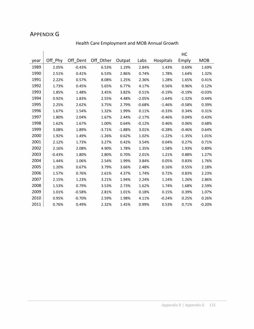
Appendix D | Appendix G 115
APPENDIX G
Health Care Employment and MOB Annual Growth
year Off_Phy Off_Dent Off_Other Outpat Labs HospitalsHC
Emply MOB
1989 2.05% ‐0.43% 6.53% 1.19% 2.84% 1.43% 0.69% 1.69%
1990 2.51% 0.41% 6.53% 2.86% 0.74% 1.78% 1.64% 1.32%
1991 2.22% 0.57% 8.08% 1.25% 2.36% 1.28% 1.65% 0.41%
1992 1.73% 0.45% 5.65% 6.77% 4.17% 0.56% 0.96% 0.12%
1993 1.85% 1.48% 3.45% 3.82% 0.51% ‐0.19% ‐0.19% ‐0.03%
1994 0.92% 1.83% 2.55% 4.48% ‐2.05% ‐1.64% ‐1.32% 0.44%
1995 2.25% 2.62% 3.75% 2.79% ‐0.68% ‐1.46% ‐0.58% 0.39%
1996 1.67% 1.54% 1.32% 1.99% 0.11% ‐0.33% 0.34% 0.31%
1997 1.80% 2.04% 1.67% 2.44% ‐2.17% ‐0.46% 0.04% 0.43%
1998 1.62% 1.67% 1.00% 0.64% ‐0.12% 0.46% 0.06% 0.68%
1999 3.08% 1.89% ‐3.71% ‐1.88% 3.01% ‐0.28% ‐0.46% 0.64%
2000 1.92% 1.49% ‐1.26% 0.62% 1.02% ‐1.22% ‐1.35% 1.01%
2001 2.12% 1.73% 3.27% 0.42% 3.54% 0.04% 0.27% 0.71%
2002 2.16% 2.08% 4.90% 1.78% 1.35% 1.58% 1.93% 0.89%
2003 ‐0.43% 1.80% 2.80% 0.70% 2.01% 1.21% 0.88% 1.27%
2004 1.44% 1.06% 2.54% 1.99% 3.84% 0.05% 0.83% 1.76%
2005 1.20% 0.67% 3.79% 3.66% 2.48% 0.16% 0.55% 2.18%
2006 1.57% 0.76% 2.61% 4.37% 1.74% 0.72% 0.83% 2.23%
2007 2.15% 1.23% 3.21% 1.94% 2.24% 1.24% 1.26% 2.86%
2008 1.53% 0.79% 3.53% 2.73% 1.62% 1.74% 1.68% 2.59%
2009 1.01% ‐0.58% 2.81% 1.01% 0.18% 0.15% 0.39% 1.07%
2010 0.95% ‐0.70% 2.59% 1.98% 4.11% ‐0.24% 0.25% 0.26%
2011 0.76% 0.49% 2.32% 1.45% 0.99% 0.53% 0.71% ‐0.20%

Appendix D | Appendix H1 116
APPENDIX H1
InDent=‐3.228 + lMSA_k + lyear_g + 0.371*lnEm_P+0.022*lnIn_P+1.18*lnPop+0.076*lnP4565_P+0.532*lnP65_P (5‐3)
Office of Dentists
Postive Trend Conservative Trend References Time Variables
MSA lnDent Dent Growth rate
lnDent Dent Growth rate
Moody's project.
2011 Moody's Growth Rate
year Historical Postive Conser.
Albany 2.8409 2.8550 20.1% 1.0241 2.7847 17.7% 2.3650 2.8550 20.7% 1988Albuquerque 4.1196 3.6100 47.4% 1.3957 4.0380 44.5% 2.7950 3.6100 29.2% 1989 ‐0.0174Atlanta 20.6717 19.7825 39.8% 3.0088 20.2624 37.1% 14.7825 19.7825 33.8% 1990 ‐0.0218Austin 7.0913 7.0850 44.4% 1.9389 6.9509 41.6% 4.9100 7.0850 44.3% 1991 ‐0.0098Baltimore 9.3532 10.9550 18.3% 2.2157 9.1680 16.0% 7.9050 10.9550 38.6% 1992 ‐0.0057Boston 24.1145 23.5100 13.4% 3.1628 23.6370 11.2% 21.2600 23.5100 10.6% 1993 0.0036Charlotte 6.4010 6.5025 29.1% 1.8365 6.2743 26.6% 4.9575 6.5025 31.2% 1994 0.0111Chicago 30.0654 28.6950 14.4% 3.3834 29.4700 12.1% 26.2825 28.6950 9.2% 1995 0.0281Cincinnati 6.9964 6.5125 22.2% 1.9254 6.8578 19.7% 5.7275 6.5125 13.7% 1996 0.0346Cleveland 7.2482 6.7900 13.0% 1.9608 7.1047 10.8% 6.4150 6.7900 5.8% 1997 0.0470Columbus 6.7689 6.5050 18.0% 1.8923 6.6349 15.6% 5.7375 6.5050 13.4% 1998 0.0539Dallas 17.5091 17.3900 26.6% 2.8427 17.1624 24.1% 13.8300 17.3900 25.7% 1999 0.0723Denver 13.1378 10.5150 43.3% 2.5555 12.8777 40.4% 9.1700 10.5150 14.7% 2000 0.0817Detroit 17.3484 16.7475 16.1% 2.8335 17.0049 13.8% 14.9400 16.7475 12.1% 2001 0.1020Edison 9.4413 9.6500 16.0% 2.2251 9.2544 13.7% 8.1400 9.6500 18.6% 2002 0.1307Fort Lauderdale 6.6641 6.0600 37.6% 1.8767 6.5322 34.9% 4.8425 6.0600 25.1% 2003 0.1509Fort Worth 8.3459 6.9075 61.4% 2.1018 8.1807 58.2% 5.1725 6.9075 33.5% 2004 0.1594Hartford 5.0770 4.8475 19.5% 1.6047 4.9765 17.2% 4.2475 4.8475 14.1% 2005 0.1553Honolulu 3.5676 3.2025 20.1% 1.2519 3.4969 17.7% 2.9700 3.2025 7.8% 2006 0.1527Houston 21.2271 19.6275 43.4% 3.0353 20.8068 40.6% 14.8000 19.6275 32.6% 2007 0.1557Indianapolis 6.5765 6.3350 17.7% 1.8635 6.4462 15.4% 5.5875 6.3350 13.4% 2008 0.1586Jacksonville 4.8737 4.0500 52.8% 1.5639 4.7772 49.8% 3.1900 4.0500 27.0% 2009 0.1655Kansas City 7.2224 6.4775 30.8% 1.9572 7.0793 28.2% 5.5200 6.4775 17.3% 2010 0.1557Las Vegas 7.4786 7.0350 42.4% 1.9920 7.3305 39.6% 5.2525 7.0350 33.9% 2011 0.1508Long Island 12.7991 12.2275 24.2% 2.5294 12.5457 21.7% 10.3075 12.2275 18.6% 2012 0.1477 0.1462Los Angeles 37.0570 32.3700 34.5% 3.5925 36.3233 31.8% 27.5600 32.3700 17.5% 2013 0.1452 0.1415Louisville 3.9372 4.0350 19.5% 1.3505 3.8592 17.1% 3.2950 4.0350 22.5% 2014 0.1424 0.1369Memphis 3.5148 3.4050 20.4% 1.2370 3.4452 18.0% 2.9200 3.4050 16.6% 2015 0.1396 0.1323

Appendix D | Appendix H1 117
Miami 8.2425 7.0350 34.6% 2.0893 8.0793 31.9% 6.1250 7.0350 14.9% 2016 0.1368 0.1277Milwaukee 5.9817 5.8375 20.8% 1.7687 5.8632 18.4% 4.9525 5.8375 17.9% 2017 0.1340 0.1231Minneapolis 13.7460 11.4275 38.6% 2.6007 13.4738 35.9% 9.9175 11.4275 15.2% 2018 0.1312 0.1185Nashville 4.8897 5.1300 14.0% 1.5671 4.7929 11.7% 4.2900 5.1300 19.6% 2019 0.1284 0.1138New York 32.8010 32.0200 11.3% 3.4705 32.1515 9.1% 29.4625 32.0200 8.7% 2020 0.1256 0.1092Newark 8.0492 8.8850 7.9% 2.0656 7.8898 5.8% 7.4575 8.8850 19.1% 2021 0.1228 0.1046Norfolk 3.5637 5.5825 ‐29.0% 1.2508 3.4931 ‐30.4% 5.0200 5.5825 11.2% 2022 0.1200 0.1000Oakland 13.1652 9.9400 53.8% 2.5576 12.9045 50.7% 8.5625 9.9400 16.1%Oklahoma City 4.6676 4.1175 23.7% 1.5206 4.5752 21.3% 3.7725 4.1175 9.1%Orange County 15.7358 14.5750 27.9% 2.7359 15.4242 25.3% 12.3075 14.5750 18.4%Orlando 8.5634 7.4975 64.1% 2.1275 8.3938 60.9% 5.2175 7.4975 43.7%Philadelphia 17.7356 17.8350 15.7% 2.8556 17.3844 13.4% 15.3350 17.8350 16.3%Phoenix 17.1003 15.1875 48.0% 2.8191 16.7617 45.0% 11.5575 15.1875 31.4%Pittsburgh 7.3509 8.3650 8.7% 1.9748 7.2053 6.6% 6.7600 8.3650 23.7%Portland 11.5093 11.8100 27.3% 2.4232 11.2814 24.8% 9.0425 11.8100 30.6%Raleigh 7.9196 7.4750 47.4% 2.0493 7.7628 44.5% 5.3725 7.4750 39.1%Richmond 4.4722 4.1150 25.8% 1.4779 4.3837 23.3% 3.5550 4.1150 15.8%Riverside 12.4432 10.7250 41.0% 2.5012 12.1968 38.2% 8.8250 10.7250 21.5%Sacramento 10.7000 8.3575 52.3% 2.3502 10.4881 49.3% 7.0250 8.3575 19.0%Salt Lake City 9.0675 8.0050 35.8% 2.1847 8.8879 33.1% 6.6775 8.0050 19.9%San Antonio 6.8415 7.0700 16.9% 1.9030 6.7060 14.6% 5.8500 7.0700 20.9%San Diego 12.3554 11.4275 35.8% 2.4941 12.1108 33.1% 9.1000 11.4275 25.6%San Francisco 10.1134 7.9250 49.7% 2.2939 9.9131 46.8% 6.7550 7.9250 17.3%San Jose 12.0060 9.8200 50.9% 2.4654 11.7683 47.9% 7.9575 9.8200 23.4%Seattle 18.9733 16.8525 42.8% 2.9230 18.5976 39.9% 13.2900 16.8525 26.8%St. Louis 8.6374 8.7300 17.2% 2.1361 8.4664 14.8% 7.3725 8.7300 18.4%Stamford 3.8987 3.6800 11.1% 1.3406 3.8215 8.9% 3.5100 3.6800 4.8%Tampa 10.1599 10.3350 44.6% 2.2984 9.9587 41.7% 7.0275 10.3350 47.1%Tucson 4.6593 3.1200 95.2% 1.5189 4.5670 91.3% 2.3875 3.1200 30.7%Tulsa 2.7243 2.8075 8.8% 0.9822 2.6703 6.6% 2.5050 2.8075 12.1%Ventura 3.5988 3.0400 39.8% 1.2606 3.5275 37.0% 2.5750 3.0400 18.1%Washington, DC 21.7416 20.0500 30.4% 3.0592 21.3111 27.8% 16.6775 20.0500 20.2%West Palm Beach 6.1945 6.0000 53.6% 1.8037 6.0718 50.6% 4.0325 6.0000 48.8%Wilmington 2.4887 2.2700 23.7% 0.8917 2.4394 21.2% 2.0125 2.2700 12.8% Average 30.6% 28.0% 21.6%

118 Appendix H2 | Appendix D
APPENDIX H2
InDent=‐3.228 + lMSA_k + lyear_g + 0.371*lnEm_P+0.022*lnIn_P+1.18*lnPop+0.076*lnP4565_P+0.532*lnP65_P (5‐3)
Office of Dentists
Continuous Growth Slow Growth References Time Variables
MSA lnDent Dent Growth rate
lnDent Dent Growth rate
Moody's project.
2011 Moody's Growth Rate
year Historical Postive Conser.
Albany 0.9734 2.6470 11.9% 1.0242 2.7848 17.7% 2.3650 2.8550 20.7% 1988Albuquerque 1.3450 3.8383 37.3% 1.3958 4.0381 44.5% 2.7950 3.6100 29.2% 1989 ‐0.0174
Atlanta 2.9581 19.2606 30.3% 3.0088 20.2631 37.1% 14.7825 19.7825 33.8% 1990 ‐0.0218
Austin 1.8882 6.6072 34.6% 1.9389 6.9511 41.6% 4.9100 7.0850 44.3% 1991 ‐0.0098
Baltimore 2.1650 8.7147 10.2% 2.2158 9.1683 16.0% 7.9050 10.9550 38.6% 1992 ‐0.0057
Boston 3.1121 22.4683 5.7% 3.1628 23.6378 11.2% 21.2600 23.5100 10.6% 1993 0.0036
Charlotte 1.7858 5.9641 20.3% 1.8365 6.2745 26.6% 4.9575 6.5025 31.2% 1994 0.0111
Chicago 3.3327 28.0130 6.6% 3.3834 29.4710 12.1% 26.2825 28.6950 9.2% 1995 0.0281
Cincinnati 1.8747 6.5188 13.8% 1.9254 6.8581 19.7% 5.7275 6.5125 13.7% 1996 0.0346
Cleveland 1.9101 6.7534 5.3% 1.9608 7.1049 10.8% 6.4150 6.7900 5.8% 1997 0.0470
Columbus 1.8416 6.3068 9.9% 1.8924 6.6351 15.6% 5.7375 6.5050 13.4% 1998 0.0539
Dallas 2.7920 16.3138 18.0% 2.8428 17.1629 24.1% 13.8300 17.3900 25.7% 1999 0.0723
Denver 2.5048 12.2410 33.5% 2.5555 12.8781 40.4% 9.1700 10.5150 14.7% 2000 0.0817
Detroit 2.7828 16.1641 8.2% 2.8335 17.0055 13.8% 14.9400 16.7475 12.1% 2001 0.1020
Edison 2.1744 8.7968 8.1% 2.2251 9.2547 13.7% 8.1400 9.6500 18.6% 2002 0.1307
Fort Lauderdale 1.8260 6.2092 28.2% 1.8768 6.5324 34.9% 4.8425 6.0600 25.1% 2003 0.1509
Fort Worth 2.0511 7.7762 50.3% 2.1018 8.1809 58.2% 5.1725 6.9075 33.5% 2004 0.1594
Hartford 1.5540 4.7305 11.4% 1.6048 4.9767 17.2% 4.2475 4.8475 14.1% 2005 0.1553
Honolulu 1.2012 3.3240 11.9% 1.2519 3.4970 17.7% 2.9700 3.2025 7.8% 2006 0.1527
Houston 2.9846 19.7780 33.6% 3.0353 20.8074 40.6% 14.8000 19.6275 32.6% 2007 0.1557
Indianapolis 1.8128 6.1275 9.7% 1.8635 6.4464 15.4% 5.5875 6.3350 13.4% 2008 0.1586
Jacksonville 1.5132 4.5410 42.4% 1.5639 4.7774 49.8% 3.1900 4.0500 27.0% 2009 0.1655
Kansas City 1.9065 6.7293 21.9% 1.9572 7.0796 28.3% 5.5200 6.4775 17.3% 2010 0.1557
Las Vegas 1.9413 6.9680 32.7% 1.9921 7.3307 39.6% 5.2525 7.0350 33.9% 2011 0.1508
Long Island 2.4787 11.9254 15.7% 2.5294 12.5461 21.7% 10.3075 12.2275 18.6% 2012 0.1415 0.1462
Los Angeles 3.5418 34.5273 25.3% 3.5925 36.3245 31.8% 27.5600 32.3700 17.5% 2013 0.1323 0.1415
Louisville 1.2998 3.6684 11.3% 1.3505 3.8593 17.1% 3.2950 4.0350 22.5% 2014 0.1231 0.1369

Appendix D | Appendix H2 119
Memphis 1.1863 3.2749 12.2% 1.2370 3.4454 18.0% 2.9200 3.4050 16.6% 2015 0.1139 0.1323
Miami 2.0386 7.6798 25.4% 2.0893 8.0795 31.9% 6.1250 7.0350 14.9% 2016 0.1046 0.1277
Milwaukee 1.7180 5.5733 12.5% 1.7687 5.8634 18.4% 4.9525 5.8375 17.9% 2017 0.0954 0.1231
Minneapolis 2.5500 12.8076 29.1% 2.6008 13.4742 35.9% 9.9175 11.4275 15.2% 2018 0.0862 0.1185
Nashville 1.5164 4.5559 6.2% 1.5672 4.7930 11.7% 4.2900 5.1300 19.6% 2019 0.0770 0.1139
New York 3.4198 30.5618 3.7% 3.4705 32.1526 9.1% 29.4625 32.0200 8.7% 2020 0.0677 0.1093
Newark 2.0149 7.4997 0.6% 2.0656 7.8901 5.8% 7.4575 8.8850 19.1% 2021 0.0585 0.1046
Norfolk 1.2001 3.3204 ‐33.9% 1.2508 3.4932 ‐30.4% 5.0200 5.5825 11.2% 2022 0.0493 0.1000
Oakland 2.5069 12.2665 43.3% 2.5576 12.9049 50.7% 8.5625 9.9400 16.1%
Oklahoma City 1.4699 4.3490 15.3% 1.5207 4.5753 21.3% 3.7725 4.1175 9.1%
Orange County 2.6852 14.6616 19.1% 2.7360 15.4247 25.3% 12.3075 14.5750 18.4%
Orlando 2.0768 7.9788 52.9% 2.1275 8.3941 60.9% 5.2175 7.4975 43.7%
Philadelphia 2.8049 16.5249 7.8% 2.8556 17.3850 13.4% 15.3350 17.8350 16.3%
Phoenix 2.7684 15.9329 37.9% 2.8191 16.7622 45.0% 11.5575 15.1875 31.4%
Pittsburgh 1.9241 6.8491 1.3% 1.9749 7.2056 6.6% 6.7600 8.3650 23.7%
Portland 2.3724 10.7236 18.6% 2.4232 11.2818 24.8% 9.0425 11.8100 30.6%
Raleigh 1.9986 7.3790 37.3% 2.0494 7.7630 44.5% 5.3725 7.4750 39.1%
Richmond 1.4272 4.1669 17.2% 1.4779 4.3838 23.3% 3.5550 4.1150 15.8%
Riverside 2.4505 11.5938 31.4% 2.5012 12.1972 38.2% 8.8250 10.7250 21.5%
Sacramento 2.2995 9.9695 41.9% 2.3503 10.4885 49.3% 7.0250 8.3575 19.0%
Salt Lake City 2.1340 8.4485 26.5% 2.1847 8.8882 33.1% 6.6775 8.0050 19.9%
San Antonio 1.8523 6.3744 9.0% 1.9030 6.7062 14.6% 5.8500 7.0700 20.9%
San Diego 2.4434 11.5120 26.5% 2.4941 12.1112 33.1% 9.1000 11.4275 25.6%
San Francisco 2.2432 9.4230 39.5% 2.2939 9.9134 46.8% 6.7550 7.9250 17.3%
San Jose 2.4147 11.1864 40.6% 2.4654 11.7686 47.9% 7.9575 9.8200 23.4%
Seattle 2.8723 17.6781 33.0% 2.9231 18.5982 39.9% 13.2900 16.8525 26.8%
St. Louis 2.0854 8.0478 9.2% 2.1361 8.4667 14.8% 7.3725 8.7300 18.4%
Stamford 1.2899 3.6325 3.5% 1.3407 3.8216 8.9% 3.5100 3.6800 4.8%
Tampa 2.2477 9.4663 34.7% 2.2985 9.9590 41.7% 7.0275 10.3350 47.1%
Tucson 1.4682 4.3412 81.8% 1.5189 4.5672 91.3% 2.3875 3.1200 30.7%
Tulsa 0.9315 2.5383 1.3% 0.9822 2.6704 6.6% 2.5050 2.8075 12.1%
Ventura 1.2099 3.3531 30.2% 1.2606 3.5276 37.0% 2.5750 3.0400 18.1%
Washington, DC 3.0085 20.2574 21.5% 3.0593 21.3118 27.8% 16.6775 20.0500 20.2%
West Palm 1.7530 5.7716 43.1% 1.8037 6.0720 50.6% 4.0325 6.0000 48.8%
Wilmington 0.8410 2.3188 15.2% 0.8918 2.4395 21.2% 2.0125 2.2700 12.8%
Average 21.7% 28.0% 21.6%
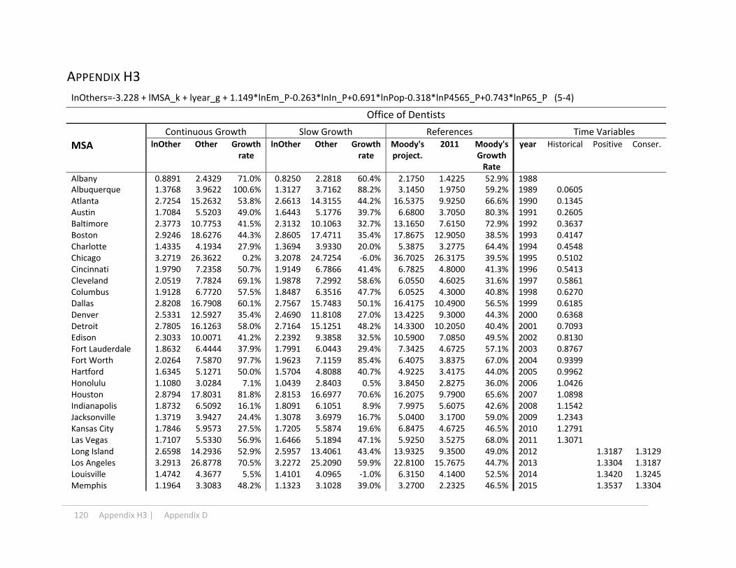
120 Appendix H3 | Appendix D
APPENDIX H3
InOthers=‐3.228 + lMSA_k + lyear_g + 1.149*lnEm_P‐0.263*lnIn_P+0.691*lnPop‐0.318*lnP4565_P+0.743*lnP65_P (5‐4)
Office of Dentists
Continuous Growth Slow Growth References Time Variables
MSA lnOther Other Growth rate
lnOther Other Growth rate
Moody's project.
2011 Moody's Growth Rate
year Historical Positive Conser.
Albany 0.8891 2.4329 71.0% 0.8250 2.2818 60.4% 2.1750 1.4225 52.9% 1988Albuquerque 1.3768 3.9622 100.6% 1.3127 3.7162 88.2% 3.1450 1.9750 59.2% 1989 0.0605 Atlanta 2.7254 15.2632 53.8% 2.6613 14.3155 44.2% 16.5375 9.9250 66.6% 1990 0.1345 Austin 1.7084 5.5203 49.0% 1.6443 5.1776 39.7% 6.6800 3.7050 80.3% 1991 0.2605 Baltimore 2.3773 10.7753 41.5% 2.3132 10.1063 32.7% 13.1650 7.6150 72.9% 1992 0.3637Boston 2.9246 18.6276 44.3% 2.8605 17.4711 35.4% 17.8675 12.9050 38.5% 1993 0.4147Charlotte 1.4335 4.1934 27.9% 1.3694 3.9330 20.0% 5.3875 3.2775 64.4% 1994 0.4548 Chicago 3.2719 26.3622 0.2% 3.2078 24.7254 ‐6.0% 36.7025 26.3175 39.5% 1995 0.5102 Cincinnati 1.9790 7.2358 50.7% 1.9149 6.7866 41.4% 6.7825 4.8000 41.3% 1996 0.5413 Cleveland 2.0519 7.7824 69.1% 1.9878 7.2992 58.6% 6.0550 4.6025 31.6% 1997 0.5861 Columbus 1.9128 6.7720 57.5% 1.8487 6.3516 47.7% 6.0525 4.3000 40.8% 1998 0.6270Dallas 2.8208 16.7908 60.1% 2.7567 15.7483 50.1% 16.4175 10.4900 56.5% 1999 0.6185Denver 2.5331 12.5927 35.4% 2.4690 11.8108 27.0% 13.4225 9.3000 44.3% 2000 0.6368 Detroit 2.7805 16.1263 58.0% 2.7164 15.1251 48.2% 14.3300 10.2050 40.4% 2001 0.7093 Edison 2.3033 10.0071 41.2% 2.2392 9.3858 32.5% 10.5900 7.0850 49.5% 2002 0.8130 Fort Lauderdale 1.8632 6.4444 37.9% 1.7991 6.0443 29.4% 7.3425 4.6725 57.1% 2003 0.8767 Fort Worth 2.0264 7.5870 97.7% 1.9623 7.1159 85.4% 6.4075 3.8375 67.0% 2004 0.9399Hartford 1.6345 5.1271 50.0% 1.5704 4.8088 40.7% 4.9225 3.4175 44.0% 2005 0.9962Honolulu 1.1080 3.0284 7.1% 1.0439 2.8403 0.5% 3.8450 2.8275 36.0% 2006 1.0426 Houston 2.8794 17.8031 81.8% 2.8153 16.6977 70.6% 16.2075 9.7900 65.6% 2007 1.0898 Indianapolis 1.8732 6.5092 16.1% 1.8091 6.1051 8.9% 7.9975 5.6075 42.6% 2008 1.1542 Jacksonville 1.3719 3.9427 24.4% 1.3078 3.6979 16.7% 5.0400 3.1700 59.0% 2009 1.2343 Kansas City 1.7846 5.9573 27.5% 1.7205 5.5874 19.6% 6.8475 4.6725 46.5% 2010 1.2791Las Vegas 1.7107 5.5330 56.9% 1.6466 5.1894 47.1% 5.9250 3.5275 68.0% 2011 1.3071Long Island 2.6598 14.2936 52.9% 2.5957 13.4061 43.4% 13.9325 9.3500 49.0% 2012 1.3187 1.3129 Los Angeles 3.2913 26.8778 70.5% 3.2272 25.2090 59.9% 22.8100 15.7675 44.7% 2013 1.3304 1.3187 Louisville 1.4742 4.3677 5.5% 1.4101 4.0965 ‐1.0% 6.3150 4.1400 52.5% 2014 1.3420 1.3245 Memphis 1.1964 3.3083 48.2% 1.1323 3.1028 39.0% 3.2700 2.2325 46.5% 2015 1.3537 1.3304
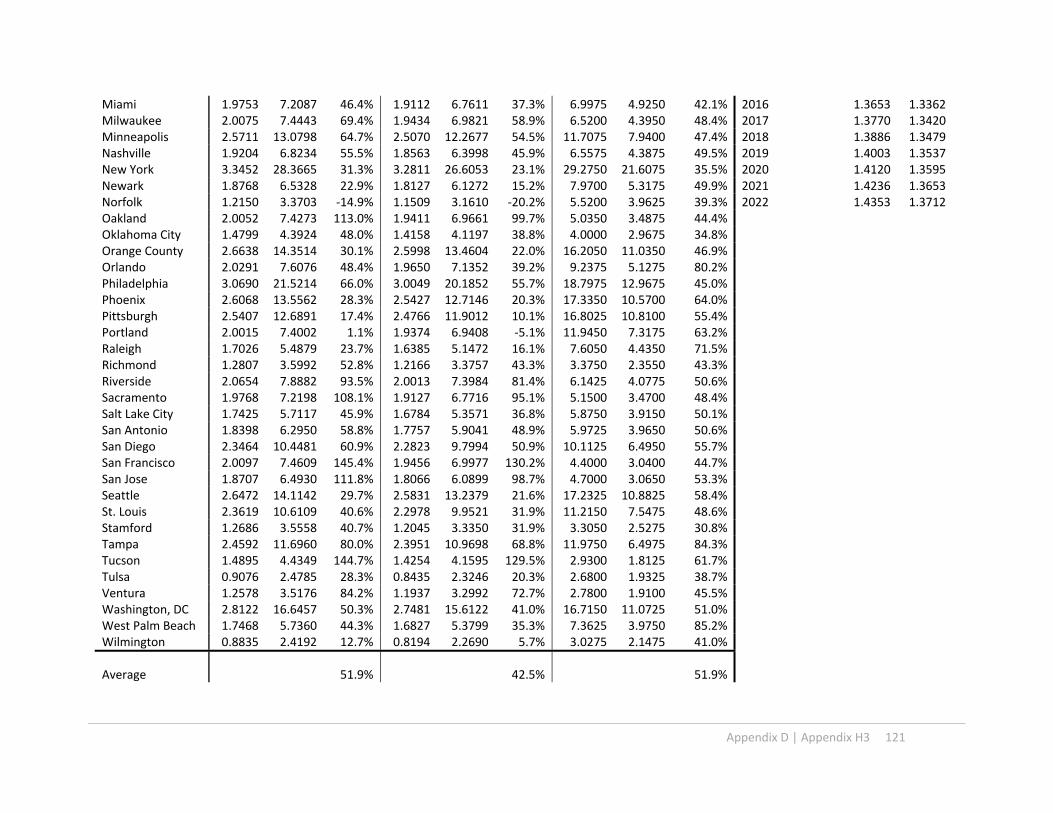
Appendix D | Appendix H3 121
Miami 1.9753 7.2087 46.4% 1.9112 6.7611 37.3% 6.9975 4.9250 42.1% 2016 1.3653 1.3362 Milwaukee 2.0075 7.4443 69.4% 1.9434 6.9821 58.9% 6.5200 4.3950 48.4% 2017 1.3770 1.3420 Minneapolis 2.5711 13.0798 64.7% 2.5070 12.2677 54.5% 11.7075 7.9400 47.4% 2018 1.3886 1.3479 Nashville 1.9204 6.8234 55.5% 1.8563 6.3998 45.9% 6.5575 4.3875 49.5% 2019 1.4003 1.3537New York 3.3452 28.3665 31.3% 3.2811 26.6053 23.1% 29.2750 21.6075 35.5% 2020 1.4120 1.3595Newark 1.8768 6.5328 22.9% 1.8127 6.1272 15.2% 7.9700 5.3175 49.9% 2021 1.4236 1.3653 Norfolk 1.2150 3.3703 ‐14.9% 1.1509 3.1610 ‐20.2% 5.5200 3.9625 39.3% 2022 1.4353 1.3712 Oakland 2.0052 7.4273 113.0% 1.9411 6.9661 99.7% 5.0350 3.4875 44.4%Oklahoma City 1.4799 4.3924 48.0% 1.4158 4.1197 38.8% 4.0000 2.9675 34.8%Orange County 2.6638 14.3514 30.1% 2.5998 13.4604 22.0% 16.2050 11.0350 46.9%Orlando 2.0291 7.6076 48.4% 1.9650 7.1352 39.2% 9.2375 5.1275 80.2%Philadelphia 3.0690 21.5214 66.0% 3.0049 20.1852 55.7% 18.7975 12.9675 45.0%Phoenix 2.6068 13.5562 28.3% 2.5427 12.7146 20.3% 17.3350 10.5700 64.0%Pittsburgh 2.5407 12.6891 17.4% 2.4766 11.9012 10.1% 16.8025 10.8100 55.4%Portland 2.0015 7.4002 1.1% 1.9374 6.9408 ‐5.1% 11.9450 7.3175 63.2%Raleigh 1.7026 5.4879 23.7% 1.6385 5.1472 16.1% 7.6050 4.4350 71.5%Richmond 1.2807 3.5992 52.8% 1.2166 3.3757 43.3% 3.3750 2.3550 43.3%Riverside 2.0654 7.8882 93.5% 2.0013 7.3984 81.4% 6.1425 4.0775 50.6%Sacramento 1.9768 7.2198 108.1% 1.9127 6.7716 95.1% 5.1500 3.4700 48.4%Salt Lake City 1.7425 5.7117 45.9% 1.6784 5.3571 36.8% 5.8750 3.9150 50.1%San Antonio 1.8398 6.2950 58.8% 1.7757 5.9041 48.9% 5.9725 3.9650 50.6%San Diego 2.3464 10.4481 60.9% 2.2823 9.7994 50.9% 10.1125 6.4950 55.7%San Francisco 2.0097 7.4609 145.4% 1.9456 6.9977 130.2% 4.4000 3.0400 44.7%San Jose 1.8707 6.4930 111.8% 1.8066 6.0899 98.7% 4.7000 3.0650 53.3%Seattle 2.6472 14.1142 29.7% 2.5831 13.2379 21.6% 17.2325 10.8825 58.4%St. Louis 2.3619 10.6109 40.6% 2.2978 9.9521 31.9% 11.2150 7.5475 48.6%Stamford 1.2686 3.5558 40.7% 1.2045 3.3350 31.9% 3.3050 2.5275 30.8%Tampa 2.4592 11.6960 80.0% 2.3951 10.9698 68.8% 11.9750 6.4975 84.3%Tucson 1.4895 4.4349 144.7% 1.4254 4.1595 129.5% 2.9300 1.8125 61.7%Tulsa 0.9076 2.4785 28.3% 0.8435 2.3246 20.3% 2.6800 1.9325 38.7%Ventura 1.2578 3.5176 84.2% 1.1937 3.2992 72.7% 2.7800 1.9100 45.5%Washington, DC 2.8122 16.6457 50.3% 2.7481 15.6122 41.0% 16.7150 11.0725 51.0%West Palm Beach 1.7468 5.7360 44.3% 1.6827 5.3799 35.3% 7.3625 3.9750 85.2%Wilmington 0.8835 2.4192 12.7% 0.8194 2.2690 5.7% 3.0275 2.1475 41.0%
Average 51.9% 42.5% 51.9%

122 Appendix H4 | Appendix D
APPENDIX H4
InOut=‐5.994 + lMSA_k + lyear_g + 0.129*lnEm_P‐0.449*lnIn_P+835*lnPop‐1.94*lnP4565_P+0.34*lnP65_P (5‐5)
Outpatient Care Centers
Continuous Growth Slow Growth References Time Variables
MSA lnOut Outpat. Growth rate
lnOther Other Growth rate
Moody's project.
2011 Moody's Growth Rate
year Historical Postive Conser.
Albany 0.8715 2.3905 28.0% 0.7402 2.0963 12.3% 2.9100 1.8675 55.8% 1988Albuquerque 2.0437 7.7192 20.5% 1.9124 6.7691 5.7% 10.4225 6.4050 62.7% 1989 0.0625 Atlanta 2.1799 8.8452 41.2% 2.0485 7.7565 23.9% 10.5575 6.2625 68.6% 1990 0.1125 Austin 0.7915 2.2068 23.8% 0.6602 1.9352 8.6% 3.2800 1.7825 84.0% 1991 0.1637 Baltimore 2.0568 7.8209 36.5% 1.9255 6.8583 19.7% 10.2050 5.7300 78.1% 1992 0.267Boston 3.2431 25.6136 45.2% 3.1118 22.4611 27.4% 24.9800 17.6350 41.7% 1993 0.2915Charlotte 1.1880 3.2806 10.6% 1.0567 2.8769 ‐3.0% 4.9925 2.9650 68.4% 1994 0.2843 Chicago 2.6404 14.0193 52.4% 2.5091 12.2937 33.6% 12.7200 9.2000 38.3% 1995 0.2944 Cincinnati 1.8549 6.3909 50.4% 1.7235 5.6043 31.9% 6.1650 4.2500 45.1% 1996 0.3012 Cleveland 1.9966 7.3642 39.6% 1.8653 6.4578 22.4% 7.0825 5.2750 34.3% 1997 0.2949 Columbus 1.5820 4.8645 55.0% 1.4506 4.2658 36.0% 4.5200 3.1375 44.1% 1998 0.3066Dallas 2.1416 8.5131 59.1% 2.0103 7.4652 39.5% 8.5700 5.3500 60.2% 1999 0.3447Denver 2.8167 16.7210 56.2% 2.6853 14.6630 36.9% 15.7100 10.7075 46.7% 2000 0.3862 Detroit 2.5975 13.4305 48.2% 2.4662 11.7774 29.9% 12.4250 9.0650 37.1% 2001 0.436 Edison 1.2201 3.3874 ‐5.6% 1.0887 2.9705 ‐17.3% 5.5300 3.5900 54.0% 2002 0.4838 Fort Lauderdale 1.1531 3.1679 1.5% 1.0217 2.7780 ‐11.0% 4.9975 3.1225 60.0% 2003 0.5254 Fort Worth 1.3812 3.9798 68.1% 1.2499 3.4900 47.4% 4.0500 2.3675 71.1% 2004 0.5858Hartford 1.1449 3.1422 19.1% 1.0136 2.7554 4.5% 3.8375 2.6375 45.5% 2005 0.6375Honolulu 0.8235 2.2785 11.0% 0.6922 1.9980 ‐2.7% 2.8025 2.0525 36.5% 2006 0.6847 Houston 2.2708 9.6870 39.2% 2.1394 8.4947 22.1% 11.8050 6.9575 69.7% 2007 0.7446 Indianapolis 1.6720 5.3226 85.0% 1.5406 4.6674 62.2% 4.0775 2.8775 41.7% 2008 0.7949 Jacksonville 1.4977 4.4715 22.6% 1.3664 3.9211 7.5% 5.9350 3.6475 62.7% 2009 0.8055 Kansas City 2.0090 7.4556 115.5% 1.8776 6.5379 89.0% 5.2175 3.4600 50.8% 2010 0.8598Las Vegas 1.6452 5.1819 104.4% 1.5138 4.5441 79.3% 4.3250 2.5350 70.6% 2011 0.8902Long Island 2.0983 8.1520 59.8% 1.9669 7.1487 40.1% 7.8350 5.1025 53.6% 2012 0.9153 0.9028 Los Angeles 3.5279 34.0539 60.8% 3.3966 29.8625 41.0% 31.5575 21.1825 49.0% 2013 0.9404 0.9153

Appendix D | Appendix H4 123
Louisville 1.6465 5.1888 28.0% 1.5152 4.5502 12.3% 6.3275 4.0525 56.1% 2014 0.9655 0.9279 Memphis 1.3813 3.9801 18.9% 1.2500 3.4902 4.3% 4.9400 3.3475 47.6% 2015 0.9906 0.9404 Miami 2.4019 11.0442 31.6% 2.2706 9.6849 15.4% 12.3675 8.3900 47.4% 2016 1.0157 0.9530 Milwaukee 2.0076 7.4454 108.7% 1.8762 6.5290 83.0% 5.4450 3.5675 52.6% 2017 1.0408 0.9655Minneapolis 2.5349 12.6147 59.9% 2.4035 11.0620 40.2% 11.9250 7.8900 51.1% 2018 1.0659 0.9781Nashville 1.9985 7.3778 51.9% 1.8671 6.4697 33.2% 7.3775 4.8575 51.9% 2019 1.0910 0.9906 New York 3.5026 33.2017 42.7% 3.3713 29.1152 25.1% 32.6825 23.2675 40.5% 2020 1.1161 1.0032 Newark 1.5245 4.5928 5.3% 1.3931 4.0275 ‐7.7% 6.6475 4.3625 52.4% 2021 1.1412 1.0157 Norfolk 2.2498 9.4857 437.4% 2.1184 8.3182 371.3% 2.5000 1.7650 41.6% 2022 1.1663 1.0283 Oakland 2.5462 12.7581 ‐23.9% 2.4148 11.1878 ‐33.2% 25.2375 16.7600 50.6%Oklahoma City 1.4978 4.4717 65.9% 1.3664 3.9213 45.5% 3.6800 2.6950 36.5%Orange County 1.8984 6.6755 54.7% 1.7671 5.8539 35.7% 6.5800 4.3150 52.5%Orlando 1.6809 5.3703 61.9% 1.5495 4.7093 42.0% 6.1150 3.3175 84.3%Philadelphia 2.9417 18.9476 31.7% 2.8103 16.6155 15.5% 21.4250 14.3875 48.9%Phoenix 3.0665 21.4660 64.5% 2.9351 18.8239 44.2% 21.9225 13.0525 68.0%Pittsburgh 1.8894 6.6152 20.2% 1.7580 5.8010 5.4% 8.6575 5.5050 57.3%Portland 2.6397 14.0094 83.7% 2.5084 12.2851 61.1% 12.5200 7.6275 64.1%Raleigh 1.2690 3.5572 34.5% 1.1376 3.1193 17.9% 4.5650 2.6450 72.6%Richmond 1.0665 2.9051 11.6% 0.9351 2.5475 ‐2.1% 3.8800 2.6025 49.1%Riverside 1.9889 7.3077 68.7% 1.8576 6.4082 47.9% 6.7775 4.3325 56.4%Sacramento 2.2812 9.7888 ‐19.5% 2.1499 8.5840 ‐29.4% 18.7325 12.1550 54.1%Salt Lake City 1.0378 2.8231 65.3% 0.9065 2.4756 45.0% 2.5900 1.7075 51.7%San Antonio 1.4525 4.2737 17.5% 1.3211 3.7477 3.0% 5.5850 3.6375 53.5%San Diego 2.3904 10.9180 206.0% 2.2591 9.5742 168.4% 5.7125 3.5675 60.1%San Francisco 2.1331 8.4413 7.0% 2.0018 7.4023 ‐6.2% 12.0450 7.8900 52.7%San Jose 1.6291 5.0991 ‐28.7% 1.4977 4.4715 ‐37.5% 11.5750 7.1500 61.9%Seattle 3.1872 24.2204 89.2% 3.0559 21.2393 65.9% 20.6625 12.8025 61.4%St. Louis 1.9466 7.0051 19.9% 1.8153 6.1429 5.1% 8.8600 5.8425 51.6%Stamford 0.2801 1.3233 59.0% 0.1488 1.1604 39.4% 1.1075 0.8325 33.0%Tampa 2.4751 11.8828 61.4% 2.3437 10.4202 41.5% 13.8675 7.3625 88.4%Tucson 1.7608 5.8170 83.2% 1.6294 5.1010 60.7% 5.1900 3.1750 63.5%Tulsa 1.2195 3.3856 168.2% 1.0882 2.9689 135.2% 1.7750 1.2625 40.6%Ventura 0.6082 1.8371 117.4% 0.4769 1.6110 90.7% 1.2300 0.8450 45.6%Washington, DC 3.0847 21.8615 64.5% 2.9534 19.1707 44.2% 20.4550 13.2900 53.9%West Palm Beach 1.4194 4.1347 65.1% 1.2881 3.6258 44.7% 4.7375 2.5050 89.1%Wilmington 0.5568 1.7450 40.4% 0.4254 1.5302 23.2% 1.8275 1.2425 47.1%
Average 55.2% 36.1% 55.2%

124 Appendix H5 | Appendix D
APPENDIX H5
InLabs=‐0.8938 + lMSA_k + lyear_g + 1.207*lnEm_P‐832*lnIn_P+1.722*lnPop+0.118*lnP4565_P+0.254*lnP65_P (5‐6)
Medical and diagnostic laboratories
Continuous Growth Slow Growth References Time Variables
MSA lnLabs Labs Growth rate
lnLabs Labs Growth rate
Moody's project.
2011 Moody's Growth Rate
year Historical Postive Conser.
Albany ‐0.8752 0.4168 71.9% ‐1.0133 0.3630 49.7% 0.3250 0.2425 34.0% 1988Albuquerque 0.8479 2.3347 34.0% 0.7098 2.0336 16.7% 2.5200 1.7425 44.6% 1989 0.0625 Atlanta 1.9897 7.3131 75.7% 1.8516 6.3701 53.0% 6.2050 4.1625 49.1% 1990 0.1125 Austin 1.1373 3.1184 102.8% 0.9992 2.7162 76.7% 2.4725 1.5375 60.8% 1991 0.1637 Baltimore 1.1397 3.1259 11.1% 1.0016 2.7228 ‐3.2% 4.4300 2.8125 57.5% 1992 0.267Boston 1.7541 5.7784 21.8% 1.6161 5.0333 6.1% 5.8325 4.7450 22.9% 1993 0.2915Charlotte 0.3268 1.3865 24.1% 0.1887 1.2077 8.1% 1.6375 1.1175 46.5% 1994 0.2843 Chicago 1.7042 5.4970 1.9% 1.5661 4.7882 ‐11.2% 6.6225 5.3950 22.8% 1995 0.2944 Cincinnati 0.4770 1.6112 9.4% 0.3390 1.4035 ‐4.7% 1.8650 1.4725 26.7% 1996 0.3012 Cleveland 0.0129 1.0130 44.2% ‐0.1252 0.8823 25.6% 0.8400 0.7025 19.6% 1997 0.2949 Columbus 0.9806 2.6660 40.1% 0.8425 2.3222 22.1% 2.4025 1.9025 26.3% 1998 0.3066Dallas 2.2314 9.3130 96.2% 2.0934 8.1121 70.9% 6.6350 4.7475 39.8% 1999 0.3447Denver 1.5848 4.8782 79.5% 1.4467 4.2491 56.4% 3.4950 2.7175 28.6% 2000 0.3862 Detroit 1.1532 3.1683 9.6% 1.0151 2.7597 ‐4.5% 3.6750 2.8900 27.2% 2001 0.436 Edison 1.4774 4.3814 36.2% 1.3393 3.8164 18.6% 4.2775 3.2175 32.9% 2002 0.4838 Fort Lauderdale 1.4463 4.2474 25.2% 1.3082 3.6997 9.1% 4.7700 3.3925 40.6% 2003 0.5254 Fort Worth 0.7817 2.1852 108.6% 0.6436 1.9034 81.7% 1.5650 1.0475 49.4% 2004 0.5858Hartford 0.3166 1.3725 36.9% 0.1786 1.1955 19.3% 1.2700 1.0025 26.7% 2005 0.6375Honolulu 0.1270 1.1354 ‐12.0% ‐0.0111 0.9890 ‐23.3% 1.5725 1.2900 21.9% 2006 0.6847 Houston 1.9630 7.1204 45.2% 1.8249 6.2022 26.5% 7.3100 4.9025 49.1% 2007 0.7446 Indianapolis 1.1935 3.2986 12.8% 1.0554 2.8733 ‐1.8% 3.7625 2.9250 28.6% 2008 0.7949 Jacksonville 0.0469 1.0480 73.9% ‐0.0912 0.9128 51.5% 0.8475 0.6025 40.7% 2009 0.8055 Kansas City 1.4834 4.4078 20.6% 1.3453 3.8394 5.0% 4.7975 3.6550 31.3% 2010 0.8598Las Vegas 1.5961 4.9335 125.0% 1.4580 4.2973 96.0% 3.2750 2.1925 49.4% 2011 0.8902Long Island 1.4581 4.2978 11.2% 1.3201 3.7436 ‐3.1% 5.1900 3.8650 34.3% 2012 0.9153 0.9028
Los Angeles 2.2224 9.2293 ‐2.4% 2.0843 8.0391 ‐15.0% 12.5575 9.4600 32.7% 2013 0.9404 0.9153
Louisville 0.2787 1.3215 94.3% 0.1407 1.1510 69.3% 0.9350 0.6800 37.5% 2014 0.9655 0.9279
Memphis 0.7032 2.0202 42.0% 0.5651 1.7597 23.7% 1.8525 1.4225 30.2% 2015 0.9906 0.9404
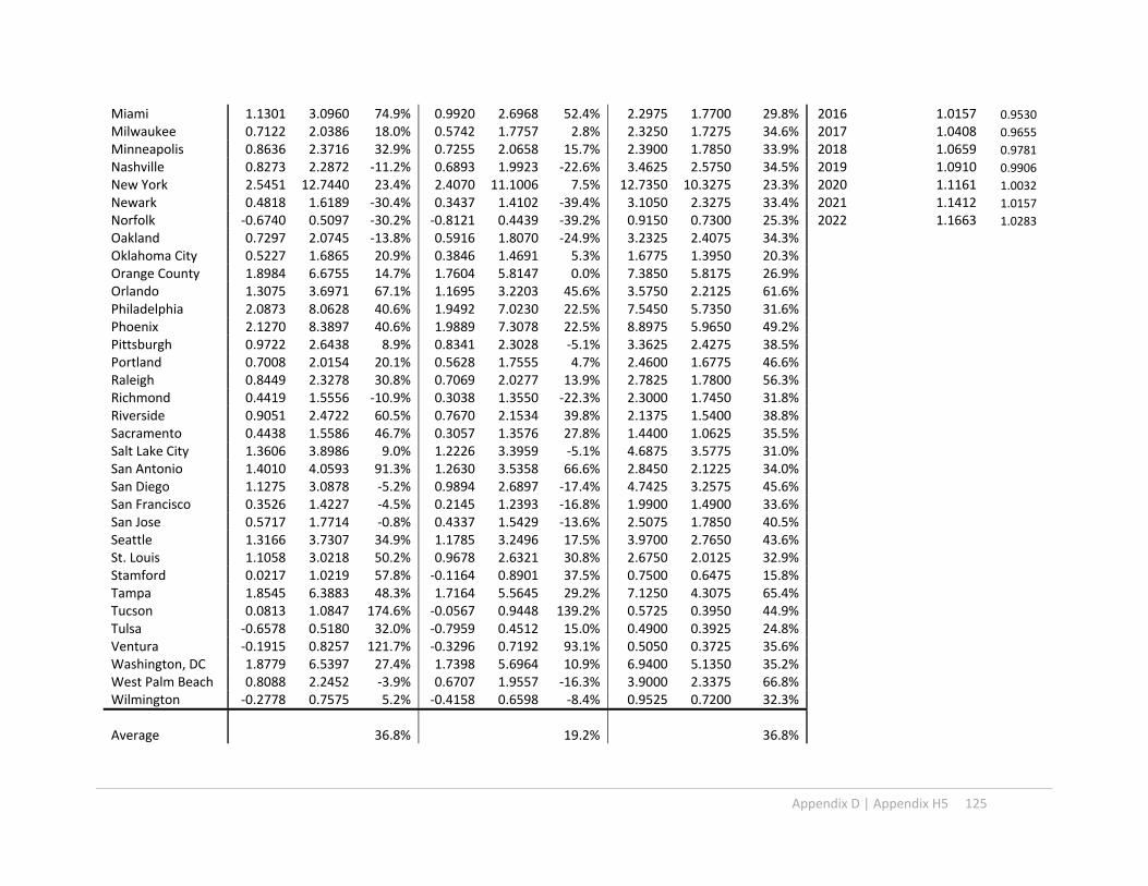
Appendix D | Appendix H5 125
Miami 1.1301 3.0960 74.9% 0.9920 2.6968 52.4% 2.2975 1.7700 29.8% 2016 1.0157 0.9530
Milwaukee 0.7122 2.0386 18.0% 0.5742 1.7757 2.8% 2.3250 1.7275 34.6% 2017 1.0408 0.9655
Minneapolis 0.8636 2.3716 32.9% 0.7255 2.0658 15.7% 2.3900 1.7850 33.9% 2018 1.0659 0.9781
Nashville 0.8273 2.2872 ‐11.2% 0.6893 1.9923 ‐22.6% 3.4625 2.5750 34.5% 2019 1.0910 0.9906
New York 2.5451 12.7440 23.4% 2.4070 11.1006 7.5% 12.7350 10.3275 23.3% 2020 1.1161 1.0032
Newark 0.4818 1.6189 ‐30.4% 0.3437 1.4102 ‐39.4% 3.1050 2.3275 33.4% 2021 1.1412 1.0157
Norfolk ‐0.6740 0.5097 ‐30.2% ‐0.8121 0.4439 ‐39.2% 0.9150 0.7300 25.3% 2022 1.1663 1.0283
Oakland 0.7297 2.0745 ‐13.8% 0.5916 1.8070 ‐24.9% 3.2325 2.4075 34.3%Oklahoma City 0.5227 1.6865 20.9% 0.3846 1.4691 5.3% 1.6775 1.3950 20.3%Orange County 1.8984 6.6755 14.7% 1.7604 5.8147 0.0% 7.3850 5.8175 26.9%Orlando 1.3075 3.6971 67.1% 1.1695 3.2203 45.6% 3.5750 2.2125 61.6%Philadelphia 2.0873 8.0628 40.6% 1.9492 7.0230 22.5% 7.5450 5.7350 31.6%Phoenix 2.1270 8.3897 40.6% 1.9889 7.3078 22.5% 8.8975 5.9650 49.2%Pittsburgh 0.9722 2.6438 8.9% 0.8341 2.3028 ‐5.1% 3.3625 2.4275 38.5%Portland 0.7008 2.0154 20.1% 0.5628 1.7555 4.7% 2.4600 1.6775 46.6%Raleigh 0.8449 2.3278 30.8% 0.7069 2.0277 13.9% 2.7825 1.7800 56.3%Richmond 0.4419 1.5556 ‐10.9% 0.3038 1.3550 ‐22.3% 2.3000 1.7450 31.8%Riverside 0.9051 2.4722 60.5% 0.7670 2.1534 39.8% 2.1375 1.5400 38.8%Sacramento 0.4438 1.5586 46.7% 0.3057 1.3576 27.8% 1.4400 1.0625 35.5%Salt Lake City 1.3606 3.8986 9.0% 1.2226 3.3959 ‐5.1% 4.6875 3.5775 31.0%San Antonio 1.4010 4.0593 91.3% 1.2630 3.5358 66.6% 2.8450 2.1225 34.0%San Diego 1.1275 3.0878 ‐5.2% 0.9894 2.6897 ‐17.4% 4.7425 3.2575 45.6%San Francisco 0.3526 1.4227 ‐4.5% 0.2145 1.2393 ‐16.8% 1.9900 1.4900 33.6%San Jose 0.5717 1.7714 ‐0.8% 0.4337 1.5429 ‐13.6% 2.5075 1.7850 40.5%Seattle 1.3166 3.7307 34.9% 1.1785 3.2496 17.5% 3.9700 2.7650 43.6%St. Louis 1.1058 3.0218 50.2% 0.9678 2.6321 30.8% 2.6750 2.0125 32.9%Stamford 0.0217 1.0219 57.8% ‐0.1164 0.8901 37.5% 0.7500 0.6475 15.8%Tampa 1.8545 6.3883 48.3% 1.7164 5.5645 29.2% 7.1250 4.3075 65.4%Tucson 0.0813 1.0847 174.6% ‐0.0567 0.9448 139.2% 0.5725 0.3950 44.9%Tulsa ‐0.6578 0.5180 32.0% ‐0.7959 0.4512 15.0% 0.4900 0.3925 24.8%Ventura ‐0.1915 0.8257 121.7% ‐0.3296 0.7192 93.1% 0.5050 0.3725 35.6%Washington, DC 1.8779 6.5397 27.4% 1.7398 5.6964 10.9% 6.9400 5.1350 35.2%West Palm Beach 0.8088 2.2452 ‐3.9% 0.6707 1.9557 ‐16.3% 3.9000 2.3375 66.8%Wilmington ‐0.2778 0.7575 5.2% ‐0.4158 0.6598 ‐8.4% 0.9525 0.7200 32.3%
Average 36.8% 19.2% 36.8%
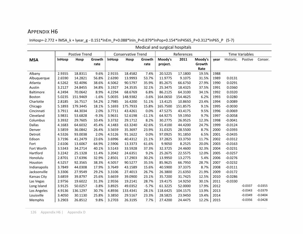
126 Appendix H6 | Appendix D
APPENDIX H6
InHosp=‐2.772 + lMSA_k + lyear_g ‐ 0.151*lnEm_P+0.088*lnIn_P+0.879*lnPop+0.154*lnP4565_P+0.312*lnP65_P (5‐7)
Medical and surgical hospitals
Postive Trend Conservative Trend References Time Variables
MSA lnHosp Hosp Growth rate
lnHosp Hosp Growth rate
Moody's project.
2011 Moody's Growth Rate
year Historic. Postive Conser.
Albany 2.9355 18.8311 9.6% 2.9155 18.4582 7.4% 20.5225 17.1800 19.5% 1988Albuquerque 2.6590 14.2821 56.8% 2.6390 13.9993 53.7% 11.9775 9.1075 31.5% 1989 0.0131 Atlanta 4.5262 92.4096 38.6% 4.5062 90.5797 35.9% 85.2675 66.6750 27.9% 1990 0.0291 Austin 3.2127 24.8455 34.8% 3.1927 24.3535 32.1% 25.3475 18.4325 37.5% 1991 0.0360 Baltimore 4.2494 70.0642 8.9% 4.2294 68.6769 6.8% 86.2125 64.3100 34.1% 1992 0.0320Boston 5.0235 151.9469 ‐1.6% 5.0035 148.9382 ‐3.6% 164.0650 154.4625 6.2% 1993 0.0280Charlotte 2.8185 16.7517 54.2% 2.7985 16.4200 51.1% 13.4125 10.8650 23.4% 1994 0.0089 Chicago 5.1893 179.3445 18.1% 5.1693 175.7933 15.8% 165.7500 151.8575 9.1% 1995 ‐0.0030 Cincinnati 3.7911 44.3034 2.0% 3.7711 43.4261 0.0% 47.5275 43.4175 9.5% 1996 ‐0.0069 Cleveland 3.9831 53.6828 ‐9.3% 3.9631 52.6198 ‐11.1% 64.9275 59.1950 9.7% 1997 ‐0.0058 Columbus 3.3932 29.7605 10.4% 3.3732 29.1712 8.2% 30.2775 26.9525 12.3% 1998 ‐0.0041Dallas 4.1683 64.6032 45.4% 4.1483 63.3240 42.6% 55.4100 44.4200 24.7% 1999 ‐0.0124Denver 3.5859 36.0842 26.4% 3.5659 35.3697 23.9% 31.0325 28.5500 8.7% 2000 ‐0.0393 Detroit 4.5326 93.0038 2.0% 4.5126 91.1622 0.0% 97.0925 91.1850 6.5% 2001 ‐0.0435 Edison 3.7196 41.2479 23.6% 3.6996 40.4312 21.1% 37.2825 33.3750 11.7% 2002 ‐0.0312 Fort 2.6106 13.6067 64.9% 2.5906 13.3373 61.6% 9.9050 8.2525 20.0% 2003 ‐0.0163 Fort Worth 3.5343 34.2714 40.1% 3.5143 33.5928 37.3% 32.3725 24.4600 32.3% 2004 ‐0.0231Hartford 3.2242 25.1328 11.4% 3.2042 24.6351 9.2% 25.2675 22.5575 12.0% 2005 ‐0.0257Honolulu 2.8701 17.6396 32.9% 2.8501 17.2903 30.2% 13.9950 13.2775 5.4% 2006 ‐0.0276 Houston 4.5257 92.3565 38.3% 4.5057 90.5277 35.5% 85.9625 66.7950 28.7% 2007 ‐0.0232 Indianapolis 3.7849 44.0308 17.9% 3.7649 43.1589 15.6% 40.5900 37.3375 8.7% 2008 ‐0.0111 Jacksonville 3.3306 27.9549 29.2% 3.3106 27.4013 26.7% 26.3800 21.6350 21.9% 2009 ‐0.0172 Kansas City 3.6859 39.8797 25.6% 3.6659 39.0900 23.1% 35.7200 31.7425 12.5% 2010 ‐0.0286Las Vegas 2.9756 19.6022 31.3% 2.9556 19.2141 28.7% 19.4175 14.9250 30.1% 2011 ‐0.0330Long Island 3.9125 50.0257 ‐3.8% 3.8925 49.0352 ‐5.7% 61.3225 52.0000 17.9% 2012 ‐0.0337 ‐0.0355
Los Angeles 4.9136 136.1297 30.7% 4.8936 133.4341 28.1% 118.6425 104.1575 13.9% 2013 ‐0.0343 ‐0.0379
Louisville 3.4050 30.1130 25.8% 3.3850 29.5167 23.3% 28.5825 23.9450 19.4% 2014 ‐0.0349 ‐0.0404
Memphis 3.2903 26.8512 9.8% 3.2703 26.3195 7.7% 27.4200 24.4475 12.2% 2015 ‐0.0356 ‐0.0428

Appendix D | Appendix H6 127
Miami 3.9131 50.0547 20.6% 3.8931 49.0636 18.2% 46.8750 41.5100 12.9% 2016 ‐0.0362 ‐0.0453
Milwaukee 3.6244 37.5032 14.4% 3.6044 36.7606 12.1% 37.5900 32.7875 14.6% 2017 ‐0.0368 ‐0.0477
Minneapolis 4.0656 58.3001 3.8% 4.0456 57.1457 1.7% 65.4700 56.1650 16.6% 2018 ‐0.0375 ‐0.0502
Nashville 3.6709 39.2887 10.1% 3.6509 38.5108 7.9% 40.6950 35.6925 14.0% 2019 ‐0.0381 ‐0.0526
New York 5.4300 228.1484 16.9% 5.4100 223.6307 14.6% 217.0275 195.1400 11.2% 2020 ‐0.0387 ‐0.0551
Newark 3.7419 42.1779 20.3% 3.7219 41.3427 17.9% 38.9875 35.0600 11.2% 2021 ‐0.0394 ‐0.0575
Norfolk 3.2624 26.1123 36.1% 3.2424 25.5952 33.4% 20.8825 19.1800 8.9% 2022 ‐0.0400 ‐0.0600
Oakland 3.5954 36.4305 45.2% 3.5754 35.7091 42.4% 28.3000 25.0850 12.8%Oklahoma City 3.2164 24.9379 23.6% 3.1964 24.4440 21.2% 21.5700 20.1750 6.9%Orange County 3.6184 37.2776 27.6% 3.5984 36.5394 25.0% 32.6250 29.2200 11.7%Orlando 3.7555 42.7547 36.6% 3.7355 41.9081 33.8% 43.8600 31.3100 40.1%Philadelphia 4.7870 119.9394 19.2% 4.7670 117.5644 16.9% 110.7775 100.5900 10.1%Phoenix 4.2291 68.6562 35.4% 4.2091 67.2968 32.7% 65.3100 50.7075 28.8%Pittsburgh 4.0417 56.9255 15.8% 4.0217 55.7983 13.5% 56.9425 49.1500 15.9%Portland 3.5971 36.4909 33.6% 3.5771 35.7683 30.9% 33.6100 27.3175 23.0%Raleigh 3.8031 44.8381 37.7% 3.7831 43.9503 35.0% 44.5525 32.5675 36.8%Richmond 2.9971 20.0273 1.4% 2.9771 19.6308 ‐0.6% 22.4225 19.7525 13.5%Riverside 3.6588 38.8140 20.9% 3.6388 38.0455 18.5% 37.7850 32.1125 17.7%Sacramento 3.1445 23.2078 7.1% 3.1245 22.7483 5.0% 25.4750 21.6675 17.6%Salt Lake City 3.1076 22.3684 35.8% 3.0876 21.9254 33.1% 17.6950 16.4725 7.4%San Antonio 3.3869 29.5741 38.4% 3.3669 28.9885 35.7% 26.2875 21.3650 23.0%San Diego 3.4612 31.8547 32.1% 3.4412 31.2240 29.5% 28.5800 24.1175 18.5%San Francisco 3.1488 23.3089 38.9% 3.1288 22.8473 36.2% 19.4150 16.7775 15.7%San Jose 3.0864 21.8987 14.9% 3.0664 21.4651 12.7% 22.4850 19.0525 18.0%Seattle 3.7565 42.7969 2.5% 3.7365 41.9495 0.5% 51.7100 41.7400 23.9%St. Louis 4.1869 65.8213 ‐4.0% 4.1669 64.5179 ‐5.9% 80.3100 68.5800 17.1%Stamford 2.6357 13.9535 3.3% 2.6157 13.6772 1.3% 13.6250 13.5075 0.9%Tampa 3.9271 50.7580 26.1% 3.9071 49.7529 23.6% 55.7850 40.2675 38.5%Tucson 3.6075 36.8741 168.9% 3.5875 36.1439 163.6% 17.2400 13.7125 25.7%Tulsa 2.7836 16.1773 ‐9.3% 2.7636 15.8570 ‐11.1% 19.4900 17.8325 9.3%Ventura 2.0240 7.5688 40.6% 2.0040 7.4189 37.8% 6.0725 5.3825 12.8%Washington, 4.4102 82.2899 20.0% 4.3902 80.6604 17.6% 79.0225 68.5975 15.2%West Palm 3.2294 25.2640 64.2% 3.2094 24.7638 61.0% 22.3700 15.3825 45.4%Wilmington 2.7727 16.0014 ‐0.1% 2.7527 15.6845 ‐2.1% 17.7500 16.0225 10.8%
Average 25.4% 22.9% 18.0%

128 Appendix I | Appendix D
APPENDIX I
Employment, Population, Income, Health Care Employment and MOB Growth Index 2011‐2022
Year Provided Projected
population population age 45‐65
Population 65+
Income per
captia
Emply per
capita
Moody's HC
Emply
Continuous growth
Slow growth
2011 1.0000 1.0000 1.0000 1.0000 1.0000 1.0000 1.0000 1.0000
2012 1.0101 1.0054 1.0347 1.0280 1.0044 1.0260 1.0230 1.0182
2013 1.0209 1.0115 1.0697 1.0661 1.0093 1.0504 1.0459 1.0364
2014 1.0320 1.0193 1.1044 1.1239 1.0229 1.0791 1.0689 1.0546
2015 1.0433 1.0285 1.1408 1.1837 1.0396 1.1131 1.0918 1.0728
2016 1.0550 1.0366 1.1768 1.2353 1.0504 1.1432 1.1148 1.0910
2017 1.0667 1.0411 1.2148 1.2717 1.0495 1.1622 1.1378 1.1092
2018 1.0785 1.0425 1.2546 1.3041 1.0437 1.1772 1.1607 1.1274
2019 1.0903 1.0423 1.2967 1.3391 1.0388 1.1940 1.1837 1.1456
2020 1.1023 1.0414 1.3416 1.3775 1.0353 1.2120 1.2066 1.1638
2021 1.1142 1.0400 1.3858 1.4186 1.0329 1.2303 1.2296 1.1820
2022 1.1261 1.0382 1.4315 1.4608 1.0305 1.2479 1.2525 1.2002
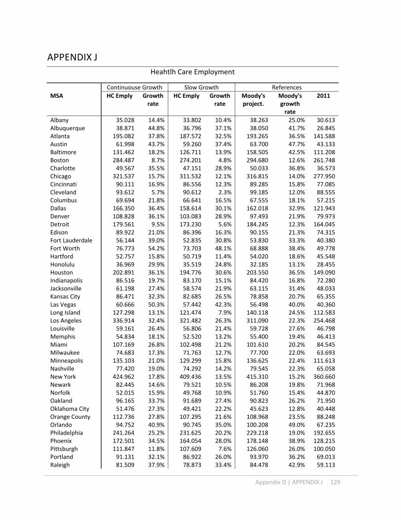
Appendix D | APPENDIX J 129
APPENDIX J
Heahtlh Care Employment
Continuouse Growth Slow Growth References
MSA HC Emply Growth rate
HC Emply Growth rate
Moody's project.
Moody's growth rate
2011
Albany 35.028 14.4% 33.802 10.4% 38.263 25.0% 30.613Albuquerque 38.871 44.8% 36.796 37.1% 38.050 41.7% 26.845Atlanta 195.082 37.8% 187.572 32.5% 193.265 36.5% 141.588Austin 61.998 43.7% 59.260 37.4% 63.700 47.7% 43.133Baltimore 131.462 18.2% 126.711 13.9% 158.505 42.5% 111.208Boston 284.487 8.7% 274.201 4.8% 294.680 12.6% 261.748Charlotte 49.567 35.5% 47.151 28.9% 50.033 36.8% 36.573Chicago 321.537 15.7% 311.532 12.1% 316.815 14.0% 277.950Cincinnati 90.111 16.9% 86.556 12.3% 89.285 15.8% 77.085Cleveland 93.612 5.7% 90.612 2.3% 99.185 12.0% 88.555Columbus 69.694 21.8% 66.641 16.5% 67.555 18.1% 57.215Dallas 166.350 36.4% 158.614 30.1% 162.018 32.9% 121.943Denver 108.828 36.1% 103.083 28.9% 97.493 21.9% 79.973Detroit 179.561 9.5% 173.230 5.6% 184.245 12.3% 164.045Edison 89.922 21.0% 86.396 16.3% 90.155 21.3% 74.315Fort Lauderdale 56.144 39.0% 52.835 30.8% 53.830 33.3% 40.380Fort Worth 76.773 54.2% 73.703 48.1% 68.888 38.4% 49.778Hartford 52.757 15.8% 50.719 11.4% 54.020 18.6% 45.548Honolulu 36.969 29.9% 35.519 24.8% 32.185 13.1% 28.455Houston 202.891 36.1% 194.776 30.6% 203.550 36.5% 149.090Indianapolis 86.516 19.7% 83.170 15.1% 84.420 16.8% 72.280Jacksonville 61.198 27.4% 58.574 21.9% 63.115 31.4% 48.033Kansas City 86.471 32.3% 82.685 26.5% 78.858 20.7% 65.355Las Vegas 60.666 50.3% 57.442 42.3% 56.498 40.0% 40.360Long Island 127.298 13.1% 121.474 7.9% 140.118 24.5% 112.583Los Angeles 336.914 32.4% 321.482 26.3% 311.090 22.3% 254.468Louisville 59.161 26.4% 56.806 21.4% 59.728 27.6% 46.798Memphis 54.834 18.1% 52.520 13.2% 55.400 19.4% 46.413Miami 107.169 26.8% 102.498 21.2% 101.610 20.2% 84.545Milwaukee 74.683 17.3% 71.763 12.7% 77.700 22.0% 63.693Minneapolis 135.103 21.0% 129.299 15.8% 136.625 22.4% 111.613Nashville 77.420 19.0% 74.292 14.2% 79.545 22.3% 65.058New York 424.962 17.8% 409.436 13.5% 415.310 15.2% 360.660Newark 82.445 14.6% 79.521 10.5% 86.208 19.8% 71.968Norfolk 52.015 15.9% 49.768 10.9% 51.760 15.4% 44.870Oakland 96.165 33.7% 91.689 27.4% 90.823 26.2% 71.950Oklahoma City 51.476 27.3% 49.421 22.2% 45.623 12.8% 40.448Orange County 112.736 27.8% 107.295 21.6% 108.968 23.5% 88.248Orlando 94.752 40.9% 90.745 35.0% 100.208 49.0% 67.235Philadelphia 241.264 25.2% 231.625 20.2% 229.218 19.0% 192.655Phoenix 172.501 34.5% 164.054 28.0% 178.148 38.9% 128.215Pittsburgh 111.847 11.8% 107.609 7.6% 126.060 26.0% 100.050Portland 91.131 32.1% 86.922 26.0% 93.970 36.2% 69.013Raleigh 81.509 37.9% 78.873 33.4% 84.478 42.9% 59.113

130 APPENDIX J | Appendix D
Richmond 45.070 11.0% 43.168 6.3% 48.718 20.0% 40.605Riverside 103.512 37.7% 98.706 31.3% 94.695 26.0% 75.170Sacramento 70.495 26.6% 67.027 20.3% 72.120 29.5% 55.705Salt Lake City 60.600 31.1% 57.896 25.2% 55.775 20.6% 46.233San Antonio 73.682 37.2% 70.214 30.8% 68.475 27.5% 53.685San Diego 97.144 35.9% 92.202 29.0% 93.393 30.7% 71.470San Francisco 67.530 47.1% 64.341 40.1% 57.970 26.2% 45.918San Jose 64.133 28.9% 61.363 23.3% 64.960 30.5% 49.770Seattle 136.841 28.1% 129.546 21.3% 143.535 34.4% 106.813St. Louis 119.436 6.8% 115.345 3.2% 136.783 22.3% 111.813Stamford 34.797 13.4% 33.292 8.5% 32.968 7.4% 30.693Tampa 124.182 33.5% 118.187 27.1% 139.673 50.2% 92.995Tucson 62.559 102.2% 60.560 95.8% 41.755 35.0% 30.935Tulsa 35.211 9.7% 33.685 5.0% 36.603 14.1% 32.085Ventura 24.341 42.7% 23.163 35.8% 20.965 22.9% 17.060Washington, DC 201.862 29.6% 192.566 23.6% 194.420 24.8% 155.770West Palm Beach 62.883 50.4% 59.999 43.5% 65.143 55.8% 41.800Wilmington 30.014 7.3% 28.960 3.5% 32.605 16.6% 27.975
Total 6636.174 6358.892 6611.745Average 28.1% 22.6% 26.4%

Appendix D | Appendix K 131
APPENDIX K
Changes from 2011‐2022 ‐ Continuous Trend Case
Changes from 2011‐2022 ‐ Slow Trend Case
MSA Off_Phy
Off_d
ent
Off_O
thers
Outpat
Labs
Hosp
Off_Phy
Off_d
ent
Off_O
thers
Outpat
Labs
Hosp
Albany ‐1.4% 0.4% 2.3% 0.4% 0.7% ‐2.4% ‐2.8% 0.7% 2.1% 0.3% 0.1% ‐0.4%
Albuquerque ‐1.4% 0.2% 2.8% ‐0.5% ‐4.0% 2.8% ‐2.0% 0.8% 2.7% ‐1.0% ‐5.5% 4.9%
Atlanta ‐2.2% 0.2% 0.8% 0.8% 0.1% 0.3% ‐3.5% 0.6% 0.6% 0.5% ‐0.3% 2.2%
Austin 1.4% 0.1% 0.3% 1.5% ‐0.6% ‐2.7% ‐0.1% 0.6% 0.1% 1.0% ‐0.9% ‐0.8%
Baltimore 2.5% 0.0% 1.3% ‐0.2% 0.8% ‐4.5% 1.3% 0.3% 1.1% ‐0.4% 0.3% ‐2.5%
Boston 1.1% 0.4% 1.6% 0.2% 2.3% ‐5.6% 0.0% 0.7% 1.4% 0.0% 1.5% ‐3.6%
Charlotte ‐1.2% ‐0.6% ‐0.5% ‐0.3% ‐1.5% 4.1% ‐2.7% 0.0% ‐0.6% ‐0.5% ‐2.0% 5.8%
Chicago ‐0.6% ‐0.1% ‐1.3% ‐0.2% 1.1% 1.1% ‐1.8% 0.2% ‐1.5% ‐0.4% 0.6% 2.9%
Cincinnati 3.6% 0.3% 1.8% ‐0.1% 1.6% ‐7.2% 2.2% 0.7% 1.6% ‐0.3% 1.0% ‐5.1%
Cleveland 3.7% 0.5% 3.1% 0.3% 1.9% ‐9.5% 2.6% 0.8% 2.9% 0.2% 1.2% ‐7.6%
Columbus 0.5% ‐0.3% 2.2% 0.5% 1.5% ‐4.4% ‐0.8% 0.1% 2.0% 0.2% 0.9% ‐2.4%
Dallas ‐5.5% ‐0.8% 1.5% 1.7% 0.7% 2.4% ‐6.9% ‐0.3% 1.3% 1.2% 0.3% 4.3%
Denver ‐1.1% 0.6% ‐0.1% 1.1% 2.0% ‐2.5% ‐2.0% 1.3% ‐0.2% 0.7% 0.8% ‐0.7%
Detroit ‐1.5% 0.6% 2.8% 0.0% 2.0% ‐3.8% ‐2.6% 0.9% 2.5% ‐0.2% 1.3% ‐1.9%
Edison ‐1.6% ‐0.5% 1.6% 0.5% ‐1.1% 1.0% ‐2.8% 0.0% 1.3% 0.1% ‐1.4% 2.8% Fort Lauderdale ‐0.7% ‐0.1% ‐0.1% ‐0.8% ‐2.1% 3.8% ‐1.9% 0.6% ‐0.1% ‐1.4% ‐2.5% 5.3%
Fort Worth 0.7% 0.5% 2.2% 0.7% 0.4% ‐4.5% ‐0.7% 0.9% 1.9% 0.5% 0.0% ‐2.6%
Hartford ‐1.2% 0.3% 2.2% 0.4% 0.2% ‐1.9% ‐2.5% 0.7% 2.0% 0.2% ‐0.4% 0.0%
Honolulu 4.0% ‐0.8% ‐1.7% ‐1.5% ‐1.1% 1.1% 2.7% ‐0.4% ‐1.9% ‐1.7% ‐1.6% 3.0%
Houston ‐3.8% 0.5% 2.2% 0.2% 0.1% 0.7% ‐5.2% 1.0% 2.0% ‐0.1% ‐0.3% 2.6%
Indianapolis ‐0.8% ‐0.1% ‐0.2% ‐0.2% 2.2% ‐0.8% ‐2.1% 0.2% ‐0.4% ‐0.6% 1.6% 1.3%
Jacksonville ‐2.0% 1.3% ‐0.2% 0.5% ‐0.3% 0.6% ‐3.5% 1.7% ‐0.3% 0.3% ‐0.9% 2.7%
Kansas City 0.0% ‐0.1% ‐0.3% ‐0.5% 3.3% ‐2.5% ‐1.2% 0.3% ‐0.4% ‐0.9% 2.6% ‐0.3%
Las Vegas 0.0% ‐0.7% 0.4% 2.7% 2.3% ‐4.7% ‐1.1% 0.0% 0.3% 2.0% 1.6% ‐2.9%
Long Island 1.3% 0.9% 2.9% ‐0.1% 1.9% ‐6.9% ‐0.1% 1.4% 2.7% ‐0.4% 1.4% ‐5.0%
Los Angeles ‐2.2% 0.2% 1.8% ‐1.0% 1.8% ‐0.5% ‐3.5% 0.7% 1.6% ‐1.2% 1.0% 1.4%
Louisville 1.2% ‐0.4% ‐1.5% 0.8% 0.1% ‐0.3% 0.0% ‐0.1% ‐1.6% 0.6% ‐0.6% 1.8%
Memphis 1.7% 0.1% 1.2% 0.6% 0.0% ‐3.7% 0.3% 0.4% 1.1% 0.3% ‐0.6% ‐1.5%
Miami ‐0.1% 0.4% 0.9% 0.8% 0.4% ‐2.4% ‐1.4% 0.8% 0.8% 0.5% ‐0.5% ‐0.3%
Milwaukee ‐6.4% 0.2% 3.1% 0.0% 4.4% ‐1.3% ‐7.4% 0.6% 2.8% ‐0.2% 3.5% 0.8%
Minneapolis 0.9% 1.3% 2.6% 0.2% 2.3% ‐7.2% ‐0.4% 1.7% 2.4% 0.0% 1.5% ‐5.2%
Nashville 1.3% ‐0.3% 2.1% ‐1.0% 2.1% ‐4.1% 0.2% 0.0% 1.9% ‐1.3% 1.2% ‐2.0%
New York ‐1.3% ‐0.5% 0.7% 0.1% 1.4% ‐0.4% ‐2.5% ‐0.2% 0.5% ‐0.2% 0.7% 1.6%

132 Appendix K | Appendix D
Newark ‐0.6% ‐0.6% 0.5% ‐1.3% ‐0.5% 2.4% ‐1.9% ‐0.2% 0.3% ‐1.5% ‐1.0% 4.3%
Norfolk ‐14.4% ‐4.3% ‐2.4% ‐0.6% 14.3% 7.5% ‐15.3% ‐4.0% ‐2.5% ‐0.7% 12.8% 9.7%
Oakland 3.5% 1.8% 2.9% ‐1.2% ‐10.0% 3.0% 2.4% 2.5% 2.8% ‐1.4% ‐11.1% 4.9% Oklahoma City ‐1.4% ‐0.3% 1.2% ‐0.2% 2.0% ‐1.4% ‐2.5% 0.1% 1.0% ‐0.5% 1.3% 0.6% Orange County ‐0.6% 0.0% 0.2% ‐0.7% 1.0% 0.0% ‐1.8% 0.7% 0.0% ‐1.2% 0.6% 1.6%
Orlando ‐1.6% 1.3% 0.4% 0.6% 0.7% ‐1.4% ‐3.0% 1.7% 0.2% 0.3% 0.3% 0.5%
Philadelphia 0.2% ‐0.6% 2.2% 0.4% 0.4% ‐2.5% ‐1.0% ‐0.3% 2.0% 0.1% ‐0.3% ‐0.4%
Phoenix ‐3.2% 0.9% ‐0.4% 0.2% 2.3% 0.3% ‐4.3% 1.4% ‐0.5% ‐0.2% 1.3% 2.3%
Pittsburgh ‐2.5% ‐0.2% 0.5% ‐0.1% 0.4% 1.8% ‐3.7% 0.1% 0.3% ‐0.3% ‐0.1% 3.8%
Portland ‐1.6% ‐0.5% ‐2.5% ‐0.2% 4.3% 0.5% ‐2.6% 0.1% ‐2.6% ‐0.4% 3.1% 2.4%
Raleigh 0.5% 0.6% ‐0.8% ‐0.2% ‐0.1% ‐0.1% ‐0.8% 1.0% ‐1.0% ‐0.4% ‐0.5% 1.8%
Richmond 1.7% 1.2% 2.2% ‐0.8% 0.0% ‐4.2% 0.3% 1.6% 2.0% ‐1.2% ‐0.5% ‐2.3%
Riverside 1.1% 0.3% 2.2% 0.3% 1.3% ‐5.2% ‐0.4% 0.9% 2.1% 0.1% 0.7% ‐3.4%
Sacramento 7.0% 2.6% 4.0% 0.3% ‐7.9% ‐6.0% 5.9% 3.4% 3.9% 0.1% ‐9.0% ‐4.3% Salt Lake City ‐2.4% 0.5% 1.0% ‐1.3% 1.0% 1.3% ‐3.7% 1.2% 0.8% ‐1.9% 0.6% 3.0%
San Antonio ‐0.5% ‐1.6% 1.2% 1.6% ‐1.0% 0.3% ‐1.8% ‐1.2% 1.0% 1.1% ‐1.4% 2.3%
San Diego ‐5.6% 0.0% 1.7% ‐1.4% 6.2% ‐1.0% ‐6.8% 0.7% 1.5% ‐1.6% 5.4% 0.8% San Francisco 3.2% 0.3% 4.4% ‐1.1% ‐4.7% ‐2.0% 2.0% 1.0% 4.3% ‐1.3% ‐5.7% ‐0.3%
San Jose 4.7% 2.7% 4.0% ‐0.8% ‐6.4% ‐4.1% 3.4% 3.6% 3.8% ‐1.1% ‐7.1% ‐2.6%
Seattle 0.4% 1.4% 0.1% 0.1% 5.7% ‐7.8% ‐0.5% 2.2% 0.0% ‐0.1% 4.4% ‐6.0%
St. Louis 2.1% 0.6% 2.1% 0.7% 0.6% ‐6.2% 0.9% 0.9% 1.9% 0.5% 0.1% ‐4.3%
Stamford 0.2% ‐0.2% 2.0% 0.8% 1.1% ‐3.9% ‐1.3% 0.3% 1.8% 0.6% 0.8% ‐2.1%
Tampa ‐2.8% 0.6% 2.4% 0.5% 1.7% ‐2.4% ‐4.0% 1.0% 2.3% 0.1% 0.9% ‐0.4%
Tucson ‐15.1% ‐0.3% 1.2% 0.5% ‐1.0% 14.6% ‐16.0% 0.0% 1.0% 0.3% ‐1.8% 16.6%
Tulsa 2.8% ‐0.1% 1.0% 0.2% 5.7% ‐9.6% 1.4% 0.3% 0.9% 0.1% 4.9% ‐7.6%
Ventura ‐6.3% ‐0.3% 3.3% 1.2% 2.6% ‐0.5% ‐7.5% 0.4% 3.0% 0.9% 2.0% 1.1% Washington, DC ‐0.2% 0.1% 1.1% ‐0.1% 2.3% ‐3.3% ‐1.4% 0.6% 1.0% ‐0.3% 1.4% ‐1.3% West Palm Beach ‐1.8% 0.2% ‐0.4% ‐2.0% 0.6% 3.4% ‐3.2% 0.7% ‐0.5% ‐2.3% 0.1% 5.3%
Wilmington 1.2% 1.1% 0.4% 0.0% 1.4% ‐4.0% ‐0.1% 1.4% 0.2% ‐0.3% 0.8% ‐2.0%

Appendix D | Appendix L1 133
APPENDIX L1 MOB=1313392 + lMSA_k + lyear_g +120880*Off_Phy+414729*Off_Dent ‐156728*Off_Others ‐ 86499 * Outpat + 307486* Labs +67467*Hosp (5‐1)
Medical Office Building
Scenario 1 Reference Time Variables
MSA 2011 MOB
MOB Growth rate
W Moody's HC Emply.
Growth rate
year Historic. Positive
Albany 5,453,962 6,492,636 19.0% 6,689,579 22.7% 1988 Albuquerque 4,774,886 7,089,831 48.5% 6,417,513 34.4% 1989 100,315
Atlanta 23,367,741 27,651,152 18.3% 26,605,266 13.9% 1990 169,235
Austin 6,338,648 9,592,875 51.3% 9,211,378 45.3% 1991 179,770
Baltimore 6,815,682 9,704,035 42.4% 11,873,776 74.2% 1992 186,867
Boston 18,236,550 21,955,065 20.4% 22,640,198 24.1% 1993 177,952
Charlotte 10,244,875 10,594,955 3.4% 10,286,696 0.4% 1994 253,423
Chicago 24,288,432 28,525,366 17.4% 27,598,750 13.6% 1995 276,852
Cincinnati 8,456,160 9,891,643 17.0% 9,642,233 14.0% 1996 282,111
Cleveland 9,806,688 10,512,560 7.2% 10,705,645 9.2% 1997 303,101
Columbus 11,324,002 12,402,697 9.5% 12,172,412 7.5% 1998 312,520
Dallas 19,593,469 23,718,037 21.1% 23,179,903 18.3% 1999 247,201
Denver 13,260,064 14,116,030 6.5% 12,167,122 ‐8.2% 2000 296,592
Detroit 32,198,639 29,973,994 ‐6.9% 30,736,032 ‐4.5% 2001 298,175
Edison 8,009,995 11,171,911 39.5% 10,788,599 34.7% 2002 287,542
Fort Lauderdale 7,830,102 10,860,919 38.7% 10,082,434 28.8% 2003 355,225
Fort Worth 20,845,076 20,522,082 ‐1.5% 19,254,990 ‐7.6% 2004 473,335
Hartford 5,766,105 7,724,141 34.0% 7,614,751 32.1% 2005 678,054
Honolulu 3,263,759 5,479,452 67.9% 4,825,915 47.9% 2006 869,711
Houston 28,127,819 31,744,152 12.9% 31,335,589 11.4% 2007 1,080,818
Indianapolis 10,844,270 12,344,947 13.8% 12,456,745 14.9% 2008 1,298,250
Jacksonville 4,544,375 7,495,795 64.9% 6,993,233 53.9% 2009 1,465,975
Kansas City 8,042,803 10,385,027 29.1% 10,054,365 25.0% 2010 1,527,107
Las Vegas 12,533,038 13,326,042 6.3% 12,582,675 0.4% 2011 1,525,325 1,525,325
Long Island 9,284,204 13,065,335 40.7% 14,141,693 52.3% 2012 1,587,249
Los Angeles 36,517,625 43,729,752 19.7% 41,970,757 14.9% 2013 1,649,172
Louisville 7,084,105 9,204,291 29.9% 8,759,658 23.7% 2014 1,711,096
Memphis 8,152,767 9,822,561 20.5% 9,535,200 17.0% 2015 1,773,020
Miami 9,958,670 12,835,188 28.9% 11,487,374 15.4% 2016 1,834,944
Milwaukee 7,639,098 8,710,205 14.0% 9,748,442 27.6% 2017 1,896,867
Minneapolis 16,512,875 17,896,961 8.4% 17,377,413 5.2% 2018 1,958,791
Nashville 7,452,794 8,606,523 15.5% 9,110,452 22.2% 2019 2,020,715
New York 18,576,417 24,520,192 32.0% 23,750,582 27.9% 2020 2,082,639
Newark 5,710,576 8,576,892 50.2% 8,980,888 57.3% 2021 2,144,562
Norfolk 5,788,962 5,857,609 1.2% 8,454,431 46.0% 2022 2,206,486
Oakland 9,448,132 12,896,809 36.5% 8,778,454 ‐7.1%
Oklahoma City 7,809,326 8,920,402 14.2% 8,496,613 8.8%
Orange County 14,922,867 19,345,690 29.6% 18,732,382 25.5%
Orlando 7,570,802 11,744,802 55.1% 11,605,452 53.3%

134 Appendix L1 | Appendix D
Philadelphia 16,168,428 19,400,538 20.0% 18,007,789 11.4%
Phoenix 20,583,252 22,597,710 9.8% 22,408,215 8.9%
Pittsburgh 8,151,062 10,404,813 27.6% 11,489,917 41.0%
Portland 8,741,725 10,736,528 22.8% 11,268,984 28.9%
Raleigh 8,758,395 11,520,764 31.5% 11,313,390 29.2%
Richmond 4,667,278 6,133,410 31.4% 6,236,796 33.6%
Riverside 12,237,119 15,382,886 25.7% 14,162,873 15.7%
Sacramento 7,144,696 9,601,017 34.4% 6,733,266 ‐5.8%
Salt Lake City 7,685,357 10,807,877 40.6% 10,354,243 34.7%
San Antonio 11,378,791 13,239,046 16.3% 12,300,618 8.1%
San Diego 13,070,580 15,776,053 20.7% 17,019,236 30.2%
San Francisco 5,704,052 8,606,131 50.9% 6,490,932 13.8%
San Jose 7,416,427 10,972,180 47.9% 8,954,869 20.7%
Seattle 20,791,466 20,341,762 ‐2.2% 20,707,043 ‐0.4%
St. Louis 9,152,267 11,211,858 22.5% 11,909,381 30.1%
Stamford 4,060,886 6,263,230 54.2% 6,034,849 48.6%
Tampa 10,244,043 13,314,464 30.0% 14,522,650 41.8%
Tucson 3,812,736 7,513,878 97.1% 5,855,889 53.6%
Tulsa 5,974,093 6,817,788 14.1% 7,251,002 21.4%
Ventura 3,193,810 5,020,333 57.2% 4,725,870 48.0%
Washington, DC 13,418,704 18,001,768 34.2% 17,236,441 28.5%
West Palm Beach 9,001,719 11,126,783 23.6% 11,442,179 27.1%
Wilmington 2,384,653 4,270,281 79.1% 4,365,800 83.1%
Average 28.5% 25.0%

Appendix D | Appendix L2 135
APPENDIX L2 MOB=1313392 + lMSA_k + lyear_g +120880*Off_Phy+414729*Off_Dent ‐156728*Off_Others ‐ 86499 * Outpat + 307486* Labs +67467*Hosp (5‐1)
Medical Office Building
Scenario 2 Reference Time Variables
MSA 2011 MOB
MOB Grow. rate
W Moody's HC Emply.
Grow. rate
year Historic. Conserv.
Albany 5,453,962 5,981,322 9.7% 6,174,603 13.2% 1988
Albuquerque 4,774,886 6,249,875 30.9% 5,902,537 23.6% 1989
Atlanta 23,367,741 27,691,326 18.5% 26,090,291 11.7% 1990
Austin 6,338,648 9,364,515 47.7% 8,696,403 37.2% 1991
Baltimore 6,815,682 9,444,606 38.6% 11,358,800 66.7% 1992
Boston 18,236,550 20,835,809 14.3% 22,125,222 21.3% 1993
Charlotte 10,244,875 10,158,932 ‐0.8% 9,771,720 ‐4.6% 1994
Chicago 24,288,432 29,078,036 19.7% 27,083,774 11.5% 1995
Cincinnati 8,456,160 9,449,752 11.7% 9,127,257 7.9% 1996
Cleveland 9,806,688 10,033,753 2.3% 10,190,669 3.9% 1997
Columbus 11,324,002 12,052,721 6.4% 11,657,437 2.9% 1998
Dallas 19,593,469 23,919,078 22.1% 22,664,927 15.7% 1999
Denver 13,260,064 13,243,960 ‐0.1% 11,652,147 ‐12.1% 2000
Detroit 32,198,639 29,692,205 ‐7.8% 30,221,056 ‐6.1% 2001
Edison 8,009,995 11,229,524 40.2% 10,273,624 28.3% 2002
Fort Lauderdale 7,830,102 10,629,353 35.7% 9,567,458 22.2% 2003
Fort Worth 20,845,076 20,319,121 ‐2.5% 18,740,014 ‐10.1% 2004
Hartford 5,766,105 7,380,859 28.0% 7,099,776 23.1% 2005
Honolulu 3,263,759 5,029,342 54.1% 4,310,939 32.1% 2006
Houston 28,127,819 31,931,208 13.5% 30,820,613 9.6% 2007
Indianapolis 10,844,270 11,932,616 10.0% 11,941,769 10.1% 2008
Jacksonville 4,544,375 6,935,082 52.6% 6,478,258 42.6% 2009
Kansas City 8,042,803 9,740,450 21.1% 9,539,390 18.6% 2010
Las Vegas 12,533,038 12,841,428 2.5% 12,067,699 ‐3.7% 2011 Long Island 9,284,204 13,081,592 40.9% 13,626,717 46.8% 2012 Los Angeles 36,517,625 42,594,049 16.6% 41,455,781 13.5% 2013 Louisville 7,084,105 8,618,290 21.7% 8,244,682 16.4% 2014 Memphis 8,152,767 9,249,473 13.5% 9,020,224 10.6% 2015 Miami 9,958,670 11,988,443 20.4% 10,972,398 10.2% 2016 Milwaukee 7,639,098 8,195,140 7.3% 9,233,466 20.9% 2017 Minneapolis 16,512,875 17,422,223 5.5% 16,862,437 2.1% 2018 Nashville 7,452,794 8,043,597 7.9% 8,595,476 15.3% 2019 New York 18,576,417 23,586,977 27.0% 23,235,606 25.1% 2020 Newark 5,710,576 8,229,728 44.1% 8,465,912 48.2% 2021 Norfolk 5,788,962 4,813,662 ‐16.8% 7,939,455 37.1% 2022 Oakland 9,448,132 11,920,724 26.2% 8,263,478 ‐12.5%
Oklahoma City 7,809,326 8,398,567 7.5% 7,981,638 2.2%
Orange County 14,922,867 19,494,669 30.6% 18,217,406 22.1%
Orlando 7,570,802 11,423,345 50.9% 11,090,477 46.5%
Philadelphia 16,168,428 19,108,193 18.2% 17,492,813 8.2%
Phoenix 20,583,252 21,398,551 4.0% 21,893,239 6.4%

136 | Appendix D
Pittsburgh 8,151,062 10,415,216 27.8% 10,974,942 34.6%
Portland 8,741,725 9,649,870 10.4% 10,754,008 23.0%
Raleigh 8,758,395 11,172,797 27.6% 10,798,414 23.3%
Richmond 4,667,278 5,678,472 21.7% 5,721,820 22.6%
Riverside 12,237,119 14,918,124 21.9% 13,647,897 11.5%
Sacramento 7,144,696 8,863,827 24.1% 6,218,291 ‐13.0%
Salt Lake City 7,685,357 10,542,764 37.2% 9,839,267 28.0%
San Antonio 11,378,791 12,898,911 13.4% 11,785,642 3.6%
San Diego 13,070,580 15,220,436 16.4% 16,504,261 26.3%
San Francisco 5,704,052 8,006,360 40.4% 5,975,956 4.8%
San Jose 7,416,427 10,577,775 42.6% 8,439,893 13.8%
Seattle 20,791,466 18,952,618 ‐8.8% 20,192,067 ‐2.9%
St. Louis 9,152,267 11,008,774 20.3% 11,394,406 24.5%
Stamford 4,060,886 5,941,360 46.3% 5,519,874 35.9%
Tampa 10,244,043 12,783,335 24.8% 14,007,674 36.7%
Tucson 3,812,736 6,879,352 80.4% 5,340,913 40.1%
Tulsa 5,974,093 6,224,349 4.2% 6,736,026 12.8%
Ventura 3,193,810 4,650,711 45.6% 4,210,894 31.8%
Washington, DC 13,418,704 17,035,637 27.0% 16,721,466 24.6%
West Palm 9,001,719 10,750,316 19.4% 10,927,204 21.4%
Wilmington 2,384,653 3,813,624 59.9% 3,850,824 61.5%
Average 22.5% 18.5%

Appendix D | Appendix L3 137
APPENDIX L3 MOB=1313392 + lMSA_k + lyear_g +120880*Off_Phy+414729*Off_Dent ‐156728*Off_Others ‐ 86499 * Outpat + 307486* Labs +67467*Hosp (5‐1)
Medical Office Building
Scenario 3 Time Variables
MSA 2011 MOB MOB Grow. rate
year Historic. Conserv.
Albany 5,453,962 5,870,925 7.6% 1988Albuquerque 4,774,886 6,230,403 30.5% 1989 100,315
Atlanta 23,367,741 23,950,201 2.5% 1990 169,235
Austin 6,338,648 7,775,693 22.7% 1991 179,770
Baltimore 6,815,682 7,821,424 14.8% 1992 186,867
Boston 18,236,550 19,686,086 7.9% 1993 177,952
Charlotte 10,244,875 9,511,884 ‐7.2% 1994 253,423
Chicago 24,288,432 24,766,880 2.0% 1995 276,852
Cincinnati 8,456,160 8,700,078 2.9% 1996 282,111
Cleveland 9,806,688 9,612,368 ‐2.0% 1997 303,101
Columbus 11,324,002 10,863,721 ‐4.1% 1998 312,520
Dallas 19,593,469 19,356,370 ‐1.2% 1999 247,201
Denver 13,260,064 12,371,910 ‐6.7% 2000 296,592
Detroit 32,198,639 28,045,273 ‐12.9% 2001 298,175
Edison 8,009,995 8,724,934 8.9% 2002 287,542
Fort 7,830,102 8,706,621 11.2% 2003 355,225
Fort Worth 20,845,076 18,974,440 ‐9.0% 2004 473,335
Hartford 5,766,105 6,627,704 14.9% 2005 678,054
Honolulu 3,263,759 4,574,272 40.2% 2006 869,711
Houston 28,127,819 27,967,809 ‐0.6% 2007 1,080,818
Indianapolis 10,844,270 10,626,173 ‐2.0% 2008 1,298,250
Jacksonville 4,544,375 6,611,219 45.5% 2009 1,465,975
Kansas City 8,042,803 8,522,982 6.0% 2010 1,527,107
Las Vegas 12,533,038 11,208,239 ‐10.6% 2011 1,525,325 1,525,325
Long Island 9,284,204 10,554,553 13.7% 2012 1,540,433
Los Angeles 36,517,625 40,117,312 9.9% 2013 1,555,541
Louisville 7,084,105 8,323,350 17.5% 2014 1,570,648
Memphis 8,152,767 8,690,904 6.6% 2015 1,585,756
Miami 9,958,670 11,504,387 15.5% 2016 1,600,864
Milwaukee 7,639,098 7,578,073 ‐0.8% 2017 1,615,972
Minneapolis 16,512,875 16,423,634 ‐0.5% 2018 1,631,079
Nashville 7,452,794 7,409,716 ‐0.6% 2019 1,646,187
New York 18,576,417 19,621,909 5.6% 2020 1,661,295
Newark 5,710,576 7,318,657 28.2% 2021 1,676,403
Norfolk 5,788,962 5,699,500 ‐1.5% 2022 1,691,510
Oakland 9,448,132 12,018,070 27.2%
Oklahoma City 7,809,326 7,900,172 1.2%
Orange County 14,922,867 16,035,639 7.5%
Orlando 7,570,802 9,761,555 28.9%
Philadelphia 16,168,428 15,846,360 ‐2.0%
Phoenix 20,583,252 19,829,251 ‐3.7%
Pittsburgh 8,151,062 8,542,034 4.8%
Portland 8,741,725 10,042,151 14.9%

138 Appendix L3 | Appendix D
Raleigh 8,758,395 10,044,209 14.7%
Richmond 4,667,278 5,069,997 8.6%
Riverside 12,237,119 13,804,624 12.8%
Sacramento 7,144,696 8,759,329 22.6%
Salt Lake City 7,685,357 8,803,032 14.5%
San Antonio 11,378,791 11,211,497 ‐1.5%
San Diego 13,070,580 14,221,743 8.8%
San Francisco 5,704,052 7,700,721 35.0%
San Jose 7,416,427 9,733,285 31.2%
Seattle 20,791,466 19,325,873 ‐7.0%
St. Louis 9,152,267 9,381,549 2.5%
Stamford 4,060,886 5,267,327 29.7%
Tampa 10,244,043 10,688,451 4.3%
Tucson 3,812,736 6,786,710 78.0%
Tulsa 5,974,093 6,227,555 4.2%
Ventura 3,193,810 4,183,483 31.0%
Washington, 13,418,704 15,488,555 15.4%
West Palm 9,001,719 9,726,746 8.1%
Wilmington 2,384,653 3,515,484 47.4%
Average 11.2%
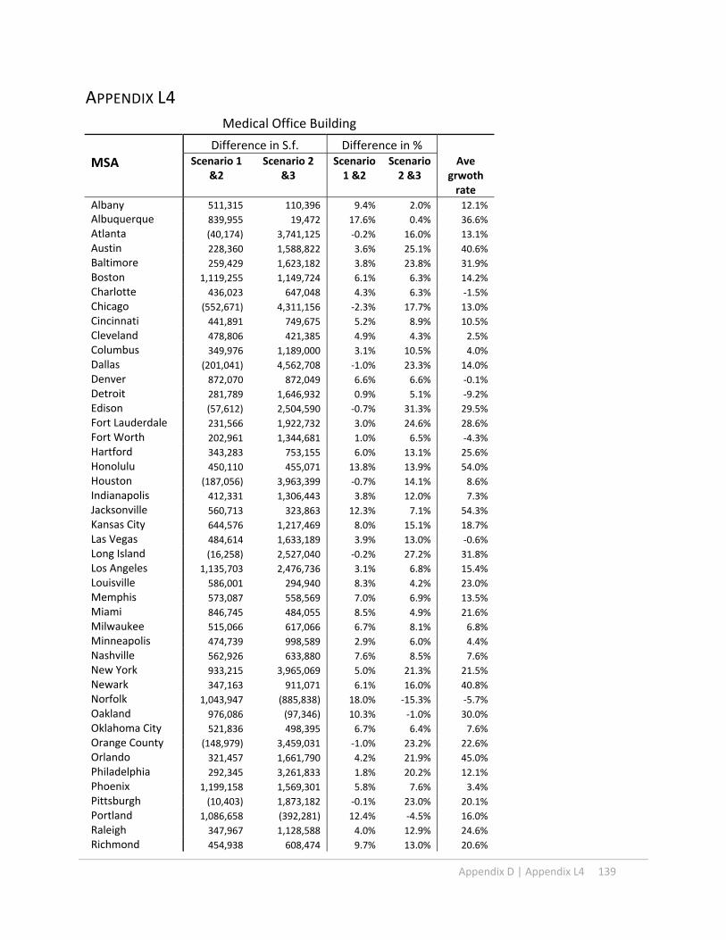
Appendix D | Appendix L4 139
APPENDIX L4
Medical Office Building
Difference in S.f. Difference in %
MSA Scenario 1 &2
Scenario 2 &3
Scenario 1 &2
Scenario 2 &3
Ave grwoth rate
Albany 511,315 110,396 9.4% 2.0% 12.1%
Albuquerque 839,955 19,472 17.6% 0.4% 36.6%
Atlanta (40,174) 3,741,125 ‐0.2% 16.0% 13.1%
Austin 228,360 1,588,822 3.6% 25.1% 40.6%
Baltimore 259,429 1,623,182 3.8% 23.8% 31.9%
Boston 1,119,255 1,149,724 6.1% 6.3% 14.2%
Charlotte 436,023 647,048 4.3% 6.3% ‐1.5%
Chicago (552,671) 4,311,156 ‐2.3% 17.7% 13.0%
Cincinnati 441,891 749,675 5.2% 8.9% 10.5%
Cleveland 478,806 421,385 4.9% 4.3% 2.5%
Columbus 349,976 1,189,000 3.1% 10.5% 4.0%
Dallas (201,041) 4,562,708 ‐1.0% 23.3% 14.0%
Denver 872,070 872,049 6.6% 6.6% ‐0.1%
Detroit 281,789 1,646,932 0.9% 5.1% ‐9.2%
Edison (57,612) 2,504,590 ‐0.7% 31.3% 29.5%
Fort Lauderdale 231,566 1,922,732 3.0% 24.6% 28.6%
Fort Worth 202,961 1,344,681 1.0% 6.5% ‐4.3%
Hartford 343,283 753,155 6.0% 13.1% 25.6%
Honolulu 450,110 455,071 13.8% 13.9% 54.0%
Houston (187,056) 3,963,399 ‐0.7% 14.1% 8.6%
Indianapolis 412,331 1,306,443 3.8% 12.0% 7.3%
Jacksonville 560,713 323,863 12.3% 7.1% 54.3%
Kansas City 644,576 1,217,469 8.0% 15.1% 18.7%
Las Vegas 484,614 1,633,189 3.9% 13.0% ‐0.6%
Long Island (16,258) 2,527,040 ‐0.2% 27.2% 31.8%
Los Angeles 1,135,703 2,476,736 3.1% 6.8% 15.4%
Louisville 586,001 294,940 8.3% 4.2% 23.0%
Memphis 573,087 558,569 7.0% 6.9% 13.5%
Miami 846,745 484,055 8.5% 4.9% 21.6%
Milwaukee 515,066 617,066 6.7% 8.1% 6.8%
Minneapolis 474,739 998,589 2.9% 6.0% 4.4%
Nashville 562,926 633,880 7.6% 8.5% 7.6%
New York 933,215 3,965,069 5.0% 21.3% 21.5%
Newark 347,163 911,071 6.1% 16.0% 40.8%
Norfolk 1,043,947 (885,838) 18.0% ‐15.3% ‐5.7%
Oakland 976,086 (97,346) 10.3% ‐1.0% 30.0%
Oklahoma City 521,836 498,395 6.7% 6.4% 7.6%
Orange County (148,979) 3,459,031 ‐1.0% 23.2% 22.6%
Orlando 321,457 1,661,790 4.2% 21.9% 45.0%
Philadelphia 292,345 3,261,833 1.8% 20.2% 12.1%
Phoenix 1,199,158 1,569,301 5.8% 7.6% 3.4%
Pittsburgh (10,403) 1,873,182 ‐0.1% 23.0% 20.1%
Portland 1,086,658 (392,281) 12.4% ‐4.5% 16.0%
Raleigh 347,967 1,128,588 4.0% 12.9% 24.6%
Richmond 454,938 608,474 9.7% 13.0% 20.6%
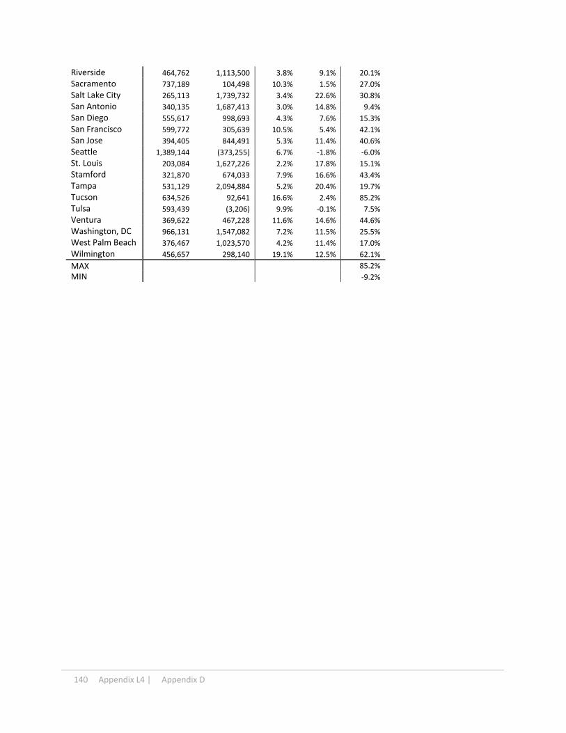
140 Appendix L4 | Appendix D
Riverside 464,762 1,113,500 3.8% 9.1% 20.1%
Sacramento 737,189 104,498 10.3% 1.5% 27.0%
Salt Lake City 265,113 1,739,732 3.4% 22.6% 30.8%
San Antonio 340,135 1,687,413 3.0% 14.8% 9.4%
San Diego 555,617 998,693 4.3% 7.6% 15.3%
San Francisco 599,772 305,639 10.5% 5.4% 42.1%
San Jose 394,405 844,491 5.3% 11.4% 40.6%
Seattle 1,389,144 (373,255) 6.7% ‐1.8% ‐6.0%
St. Louis 203,084 1,627,226 2.2% 17.8% 15.1%
Stamford 321,870 674,033 7.9% 16.6% 43.4%
Tampa 531,129 2,094,884 5.2% 20.4% 19.7%
Tucson 634,526 92,641 16.6% 2.4% 85.2%
Tulsa 593,439 (3,206) 9.9% ‐0.1% 7.5%
Ventura 369,622 467,228 11.6% 14.6% 44.6%
Washington, DC 966,131 1,547,082 7.2% 11.5% 25.5%
West Palm Beach 376,467 1,023,570 4.2% 11.4% 17.0%
Wilmington 456,657 298,140 19.1% 12.5% 62.1%
MAX 85.2%
MIN ‐9.2%