Wei Tian Miaojie Yu September 2, 2015

No.E2015003 September 2015

Distribution, Outward FDI, and Productivity Heterogeneity:

Evidence from Chinese Firms

Wei Tian Miaojie Yu

September 2, 2015

Distribution, Outward FDI, and Productivity Heterogeneity:Evidence from Chinese Firms�

Wei Tiany Miaojie Yuz

September 2, 2015

Abstract

This is the �rst paper to examine distribution-oriented outward FDI using Chinese multi-

national �rm�level data. Distribution outward FDI refers to Chinese parent �rms in man-

ufacturing that penetrate foreign markets through wholesale trade a¢ liates that resell ex-

portable goods. Our estimations correct for rare-events bias and show that distribution

FDI are more (less) productive than non-FDI (non-distribution FDI) �rms. As cross-border

communications costs (transportation costs) increase, there is a higher the probability that

�rms engage in distribution FDI (non-distribution FDI). Our endogenous income-threshold

estimates show that high-productivity Chinese �rms invest more in high-income countries,

but not necessarily in low-income countries.

JEL: F13, O11, P51

Keywords: Distribution FDI, Firm Productivity, Linder Hypothesis, Rare-Events Cor-

rections, Threshold Estimates

�We thank seminar and conference participants of HKUST, Keio, Gakushuin, Nankai, Leuven, Hitotsubashi,the 17 NBER-CCER Annual Conference and the 1st Comparative Economics World Congress for their helpfulcomments and suggestions. We appreciate Hitotsubashi Institute of Advanced Studies for generous hosting.However, all errors are ours.

ySchool of International Trade and Economics, University of International Business and Economics, Beijing,China. Email: [email protected].

zCorresponding author. China Center for Economic Research (CCER), National School of Development,Peking University, Beijing 100871, China. Phone: +86-10-6275-3109, Email: [email protected].

1 Introduction

Distribution-oriented outward foreign direct investment (FDI) refers to the phenomenon of home

parent manufacturing �rms that penetrate foreign markets through wholesale trade a¢ liates

that resell exportable goods. Distribution-oriented outward FDI is an important phenomenon

in developed countries like the United States (Hanson et al. 2001), and in developing countries

like China. However, there is relatively scant research on this topic. The present paper aims to

�ll this gap.

Outward FDI can be broken down into two main categories: distribution-oriented and non-

distribution production-oriented FDI. Distribution FDI includes the business-service foreign

a¢ liates and the wholesale foreign a¢ liates. The business-service FDI mainly refers to building

overseas business o¢ ce to explore foreign market, to promote sales, and to serve customers in

the hosting countries. Similarly, the wholesale FDI refer to oversea intermediaries of parent

�rms to help exporting and sales in the host countries.

In the United States, the wholesale foreign a¢ liates accounted for over 20% of total foreign

sales by multinationals even in a decade ago. The number of wholesale foreign a¢ liates is

around 50 percent of that of production foreign a¢ liates. In a developing country like China,

the proportion of distribution FDI is even higher. According to the report by the Ministry of

Commerce (MOC 2013), China�s outward FDI has increased dramatically in the new century.

China�s outward FDI �ow accounts for 7.6 percent of global FDI �ow and ranks third in the

world, following the United States and Japan, and �rst among developing countries. More

importantly, the share of China�s distribution outward FDI increased from around 28 percent

in 2004 to around 40 percent in 2013. The FDI stock in the business-service sector accounts for

roughly 30% of the total FDI in 2013, ranking top in all industries. The wholesale FDI ranks

fourth and accounts for 14% of the total FDI stock. By sharp contrast, production FDI only

accounts for 6% in the same period. In addition, distribution FDI is highly correlated with �rm

exports and has distinct characters from those of production FDI.

This raises two questions. First, compared with building production plants overseas, why is

distribution outward FDI so popular? What causes some �rms to engage in distribution outward

FDI? Second, which investment characteristics in the host country matter for �rms to engage

in distribution FDI?

Previous pioneering works such as Hanson et al. (2001) and Horstmann and Markusen (1996)

1

make signi�cant e¤orts for us to understand the characteristics of distribution FDI. However,

we are not still entirely clear why some �rms choose distribution FDI while others do not, and

why distribution FDI is more popular in some countries like China than in other countries.

The present paper seeks to answer such questions. We argue that distribution FDI plays an

important auxiliary but signi�cant role to boost China�s exports. In accompany with China�s

fast productivity growth in the new century (Feenstra et al., 2014), distribution FDI provides a

cheaper alternative for a bunch of Chinese exporting �rms to realize the cost-saving e¤ects in

reducing the cross-border communication costs.

The current paper presents four main �ndings. First, �rms with distribution outward FDI are

found to be more productive than non-FDI �rms, but less productive than non-distribution FDI

�rms. These �ndings imply that the popularity of distribution outward FDI may be attributed

to the fact that most Chinese exporting �rms are insu¢ ciently productive to set up overseas

production lines. As a compromise, they set up a service or distribution center abroad to promote

exports. This �nding echoes the stylized fact that China�s exports have increased rapidly in the

new century (even with the appreciation of the RMB since 2005). In addition, we �nd strong

sorting behavior between production FDI, distribution FDI, and non-FDI exports. To explain

these �ndings, inspired by Oldenski (2012), we extend the model of Helpman et al. (2004) to

understand this sorting behavior. Our estimates are based on a comprehensive FDI decision

data set covering all Chinese FDI manufacturing �rms during 2000-08. However, it is important

to stress that only a very small proportion of �rms in our large sample engaged in FDI activity.

Thus, the standard nonlinear binary estimates would have downward estimation bias (King and

Zeng 2001). We thus correct for such rare-events estimation bias in the paper.

Second, we distinguish the cross-border communications costs that occur during distribu-

tion and sales (like the costs of import procedures, promoting goods, and services before and

after sales) from the usual transportation costs (i.e., iceberg transportation costs and tari¤s) to

demonstrate the importance of distribution outward FDI for exporting �rms. We �nd that the

higher are the cross-border communications costs, the higher is the probability that �rms en-

gage in distribution outward FDI. By contrast, the higher are the iceberg transportation costs,

the higher is the probability that �rms engage in non-distribution (or production) outward

FDI. These �ndings are intuitive in the sense that, by setting up a business o¢ ce or wholesale

and retail subsidiary, the �rm can largely reduce the asymmetric rent charged by local agents

2

(Horstmann and Markusen 1996). By contrast, �rms can save on transportation costs when

exporting is replaced by production FDI. These �ndings are also highly consistent with our

theoretical predictions.

Third, by allowing for �rm heterogeneity in choosing host destinations, we �nd that the role

of a �rm�s productivity in its FDI �ow di¤ers by destination income. Highly productive �rms are

more likely to invest in rich countries, but not necessarily in poor countries. This �nding persists

when we check the intensive margin of the Linder hypothesis that rich countries receive more

FDI �ows. By estimating an endogenous threshold of income in host countries, our threshold

regressions �nd support for the Linder hypothesis on FDI volume to high-income countries.

Fourth, we �nd strong evidence on the intensive margin of distribution-oriented FDI. We

�nd that �rm productivity signi�cantly boosts distribution FDI �ow once �rms self-select into

distribution FDI. Di¤erent from previous studies on Chinese outward FDI, we were able to

obtain con�dential information on the outward FDI �ow for total FDI �ow and distribution

FDI �ow in Zhejiang province, one of the most important FDI provinces in China. This is a

novel �nding in the literature on understanding China�s outward FDI, as the publicly released

nationwide FDI decision data set has the substantial pitfall that data on �rms�FDI �ows are

unavailable.

The paper makes the following four contributions to the literature. First, it enriches the

understanding of distribution outward FDI. As documented by Boatman (2007), as distribution

FDI does not save production costs, distribution FDI has received little attention in the liter-

ature from theoretical and empirical works, except a few exceptions, such as Horstmann and

Markusen (1996), Hanson et al. (2001), and Kimura and Lee (2006). We show that distribution

FDI is complementary to �rm export as a type of downward vertical FDI. As illustrated in our

theoretical framework, �rms face a trade-o¤ between variable cost and �xed cost. Firms engaged

in exporing without FDI, regardless of distribution or production orientation, bear an additional

variable cost of cross-border communications (Oldenski 2012). However, �rms engaged in dis-

tribution FDI have a larger �xed cost. The trade-o¤ between variable cost and �xed cost can be

interpreted as a new form of the standard concentration-proximity trade-o¤. Thus, productivity

heterogeneity plays an important role in understanding distribution FDI. Only highly productive

�rms would self-select into distribution FDI.

Second, the paper enriches the understanding of China�s distribution FDI. Di¤erent from

3

China�s exports, on which there is already a fairly large micro-level literature (see Qiu and

Xue (2014) for a recent survey), few papers have investigated China�s FDI, especially from

the �rm-level perspective, despite that China�s FDI �ows have become the third largest in the

world. Even for the extensive margin of China�s FDI, it has been only recently that China�s

government (more precisely, the Ministry of Commerce) has released universal, nationwide, �rm-

level FDI decision data (i.e., which �rms engage in FDI activity). With this data set, we are now

able to explore whether the well-accepted Melitz-type e¤ects apply to China. Based on Melitz

(2003), Helpman et al. (2004) predict that to enter foreign markets through foreign a¢ liates,

�rms have to pay extra high �xed costs to cover additional expenses, such as investigating the

regulatory environment in the foreign market. Only pro�table, high-productivity �rms can do

so. Our binary estimates �nd that the sorting predictions among non-FDI, distribution FDI,

and production FDI work well in China. Thus, di¤erent from the mixed �ndings on Chinese

exports and �rm productivity,1 we con�rm that the sorting behaviors among domestic sales,

exporting, and FDI proposed by Helpman et al. (2004) apply to Chinese FDI �rms.

Third and more importantly, we explore the intensive margin of �rm FDI �ows (on all FDI

and distribution FDI), which is almost completely absent in previous studies because of the

unavailability of data. As introduced in detail in the next section, although the Ministry of

Commerce of China released the list of FDI �rms (henceforth, the FDI decision data set), the

data set does not report each �rm�s FDI volume in all years. To overcome this data challenge,

we accessed a con�dential FDI data set compiled by the Department of Commerce in Zhejiang

province, which reports �rms�FDI volume in addition to all other information covered in the

FDI decision data set. Thanks to this novel data set, we are able to explore the intensive margin

of �rm FDI in China.

Finally, the paper contributes to the literature on empirical identi�cation. We adopt razor-

edge econometric techniques to deal with the related empirical challenges; the techniques can be

applied to other projects facing a similar problem or data constraints. An empirical challenge is

rare-events estimation bias. As there are much fewer FDI �rms than non-FDI �rms in our FDI

data sets (i.e., the nationwide FDI decision data and Zhejiang�s FDI �ow data), conventional

1Lu (2010) �nds that Chinese exporters are less productive. However, Dai et al. (2012) and Yu (2015) argue

that that �nding was because of the presence of China�s processing exporters, which are less productive than

non-exporters and non-processing exporters. Once processing exporters are excluded, Chinese exporters are more

productive than non-exporters, in line with the theoretical predictions of Melitz (2003).

4

binary estimates, like logit or probit, would face a downward estimation bias of �rms� FDI

probability, which will be discussed carefully. We adopt the rare-events logit method proposed

by King and Zeng (2001, 2002) to correct for possible estimation bias. We �nd that the marginal

e¤ect of �rm productivity on FDI probability with rare-events corrections is much larger than

that without the corrections, especially for the Zhejiang subsample.

Another novel econometric application is that we use the endogenous threshold regressions

developed by Hansen (1999, 2000). Recent studies �nd that the conventional Linder (1961)

export hypothesis can extend to and work for FDI: high-income countries usually absorb more

FDI (Fajgelbaum et al. 2011). We are particularly interested in whether �rm productivity has

a heterogeneous impact on �rm distribution FDI volume by destination income. The empirical

challenge is where to set the line for high-income and low-income host countries. We take a

di¤erent approach from previous studies that set the cuto¤ lines at a predetermined level as

adopted from the World Bank. We instead allow �rms to choose their endogenous cuto¤s based

on their productivity performance. Hence, we are able to estimate the endogenous average

income threshold for �rms�FDI decision. Our threshold regressions �nd strong support for the

Linder hypothesis for FDI volume to high-income countries.

The present study is related to four strands of the literature on FDI. The �rst strand is �rm

heterogeneity of productivity and FDI. Inspired by Melitz (2003), Helpman et al. (2004) develop

the concentration-proximity trade-o¤ initiated by Markusen (1984) to �nd �rms�sorting behav-

ior: low-productivity �rms self-select to sell in domestic markets, whereas high-productivity

�rms sell in domestic and foreign markets. However, only the most productive �rms self-select

to engage in FDI. The sorting pattern is mainly determined by the trade-o¤ between transporta-

tion costs and the �xed costs of FDI. By assuming that �rm production requires headquarter

services and manufactured components, Antràs and Helpman (2004) ascertain that a �rm�s pro-

ductivity ranking in�uences the �rm�s choice between outsourcing and FDI, which is con�rmed

by Federico (2009), who uses Italian manufacturing �rm-level data. Yet, the sorting pattern

proposed by Helpman et al. (2004) is challenged by Bhattacharya et al. (2010), who use data

on the Indian software industry. Di¤erent from those �ndings in the services industry, we �nd

that the predictions of Helpman et al. (2004) work well for Chinese �rms. In particular, �rms

engaged in distribution FDI are more productive than non-FDI �rms.

The second strand is related to the literature on the nexus between distribution-oriented and

5

production-oriented FDI. Horstmann and Markusen (1996) is the pioneering work on distribution

FDI. They argue that �rms have two options in foreign markets: export or distribution FDI.

Exporters need to �nd a local agent to explore the size of the market. However, this may

generate asymmetric information. Foreign local agents have an information advantage over

home exporters, as the �rm�s e¤ort and information on market size are private information.

Thus, home exporters have to pay additional information rent. By contrast, building a wholly-

owned distribution a¢ liate requires extra �xed costs. So �rms will make decisions by considering

the trade-o¤ between the two. Di¤erent from Horstmann and Markusen (1996), Hanson et al.

(2001) implicitly assume that �rm export and distribution-oriented FDI are complementary, as

distribution FDI is set up to promote exports. They compare the trade-o¤ between distribution-

and production-oriented FDI and �nd that �rms operating in countries with high income tax

would prefer distribution FDI rather than production FDI, to avoid paying the high corporate

tax. Our paper is in line with Hanson et al. (2001), in searching for the trade-o¤ among

exporting, distribution FDI, and production FDI.

The third strand is related to the literature on the nexus between exports and FDI. Early

works, such as Froot and Stein (1991), �nd that depreciation in the host country would absorb

more FDI because of the declining investment cost in the host countries. In search of the rela-

tionship between exports and FDI, Blonigen (2001, 2005) �nds a possible substitution between

Japanese FDI to the United States and Japanese exports of �nal goods to the United States in

the automobile market, although intermediate goods are complementary. Recent works exam-

ine this nexus beyond the traditional concentration-proximity models. For instance, Oldenski

(2012) explores the role of communication of complex information in the traditional proximity-

concentration model of the decision between exports and FDI. She �nds evidence that �rms

would prefer exporting if the activities require complex within-�rm communication. Instead,

�rms would prefer FDI if the goods and services require direct communication with consumers.

Based on Russ (2007), Ramondo et al. (2013) �nd that countries with less volatile �uctuations

are served relatively more by foreign a¢ liates than by exporters. Similarly, inspired by Jovanovic

(1982), Conconi et al. (2014) �nd that �rms are more likely to export rather than engage in FDI

when they face uncertainty about foreign market demand. So exporting and (horizontal) FDI

may be complements in a dynamic setup, although they are substitutes in the static setting.

The last related strand of the literature is research on China�s FDI. Because of the unavail-

6

ability of micro-level data, previous works have examined the industrial characteristics of FDI

but abstracted away the role of �rm activity. Huang and Wang (2011) argue that Chinese FDI

�rms have di¤erent objectives for their investment. Echoing this, Kolstad and Wiig (2012) �nd

that Chinese FDI is attracted to three destinations: countries with lower institutional quality,

countries that are rich in natural resources, and large markets. Most recent, related works tend

to explore what determines the FDI of Chinese �rms. Using the same universal nationwide FDI

decision data set, Wang et al. (2012) �nd that government support and the industrial structure

of Chinese �rms play an important role in interpreting the FDI decision of Chinese �rms. Re-

cently, Wang et al. (2015) use China�s �rm-level data and �nd that access to external �nance

increases the probability that �rms engage in outward FDI. Chen and Tang (2014) also �nd that

�rm productivity and the probability of �rm FDI are positively correlated; yet, because of lack

of data, they remain silent on the intensive margin of �rms�FDI. The present paper aims to �ll

this gap and take a step further to explore the income heterogeneity of �rms�FDI.

The rest of the paper is organized as follows. Section 2 extends Melitz et al. (2004) to

show sorting equilibrium by productivity heterogeneity. Section 3 describes our data sample,

followed by a careful scrutiny of measures of �rm productivity. Section 4 examines the role of

�rm productivity in the �rm�s FDI decision. Section 5 explores the intensive margin of FDI

�ows. Section 6 discusses the �rm�s investment destination and Section 7 concludes.

2 Model

We construct a theoretical framework by extending Helpman et al. (2004) to capture the behav-

ior of distribution FDI. We assume that each country has a representative constant elasticity of

substitution utility function as follows:

U = (

Zx(')

��1� d')

��1

where x(') is the consumption of product ', and � > 1:

Each �rm in country i produces one product using labor as the only input, and the �rm

has a random labor productivity ' following Pareto distribution, where Pr(' > x) = ( bx)k; k >

��1; b > 1. So 1' is the variable production cost for each unit of goods produced. The �rm �rst

decides whether to enter the market. If entry, a sunk cost of fE is required. After the entry, the

�rm observes his productivity '. to set up the production plant. If the �rm would like to serve

7

foreign countries, there are three possible ways: (1) export without any foreign investment, (2)

export but at the same time set up a foreign a¢ liate to promote exports, and (3) set up a foreign

plant to produce and sell overseas. The �rm must pay a �xed cost fX for the �rst choice; a �xed

cost fX +fS for the second choice, where fS is the up-front cost to set up a foreign a¢ liate; and

a �xed cost fM for the third choice to build a foreign plant. Here we assume that the �xed costs

satisfy the following ranking fM > fX + fS > fX > fD.2 We will validate these assumptions in

the empirical part of the paper as well.

An iceberg transportation cost � ij > 1 is needed for export, which means � ij units of product

are required for one unit sold in country j. But if the �rm builds a distribution a¢ liation, the

transportation cost may be reduced to �� ij , 0 < � < 1; �� ij > 1. The discount factor �

captures the cost reduction of investing in a trading subsidiary, which allows �rms to distribute

their products independently.

Oldenski (2012) points out that the expenses incurred during communications between the

domestic �rm and foreign customers are crucial when �rms are making the decision whether to

export or build an overseas plant. It is important to distinguish cross-border communications

costs from transportation costs. Cross-border communications cost are incurred after the goods

are transported to the destination and can be reduced by setting up a local business o¢ ce, that

is, distribution FDI, which makes the import procedure and service more e¤ective. However,

transportation costs can be only phased out when the goods are no longer imported but produced

locally, that is, via production FDI. Another di¤erence is that cross-border communications

costs are irrelevant to �rm productivity, since those costs are incurred after the transportation.

Transportation costs are iceberg costs, which vary across �rms with di¤erent productivity.

To capture these aspects, similar to Berman et al. (2012), we introduce a linear cross-border

communication cost in our model. We assume that �rms that only export have to pay �j units

of labor for the communications costs additional to production costs, but those who build an

overseas distribution foreign a¢ liate do not. The value of �j captures the cost-saving e¤ects from

establishing a business o¢ ce, which helps �rms to serve foreign customers by promoting sales

and improving after-sales services. In this way, a destination country with a poor doing-business

2Note that �xed costs for production FDI can be decomposed into two components: �xed cost for production(fPM ) and �xed cost for setting up the �rm�s own distribution center (fS) which is similar to the �xed cost ofdistribution FDI. As an usual assumption in the literature, �xed cost for production in production-type FDI isassumed to be higher than its counterpart for exports: fPM > fX . We thus have fM = fPM + fS > fX + fS .

8

environment may be associated with a poor record in enforcing contracts, which would generate

more communications costs. Di¤erent from production FDI, which saves transportation costs,

distribution FDI mainly reduces the cross-border communications costs incurred.

As in Helpman et al. (2004), wages (w) are equal to unity across countries by introducing

a homogenous good sector in which one unit of labor is used to produce one unit of output.

The homogenous good can be traded freely and an exogenous fraction of income is spent on it.

The marginal cost for each product sold, MCd = w' ;MC

e =� ijw' + �jw;MC

s =�� ijw' ;MCm =

wj' , represents the marginal cost for selling in the domestic market, exporting without foreign

investment, exporting as well as distribution investment, and building a foreign production plant.

The derived demand for product ' is

Xj(') = LjP��1j [pcj(')]

��

where Lj is labor income in country j, pcj(') =��1MC

c; c = d; e; s;m is the price of product

' if it is sold domestically, exported without a foreign distribution a¢ liate, exported with a

distribution a¢ liate, and exported with a production a¢ liate, respectively. Pj is the aggregate

price level in which its exact expression is shown in Appendix A. Inspired by Berman et al.

(2012), the pro�ts for domestic sales, exports, distribution FDI, and production FDI are as

follows:

�di = (1

')1��Bi � fD (1)

�eij = (� ij'+ �j)

1��Bj � fX (2)

�sij = (�j� ij

')1��Bj � fX � fS (3)

�mij = (1

')1��Bj � fM , (4)

where Bj = 1�

��1

�1��LjP

��1j . The productivity cut-o¤ points satisfy �di = 0; �eij =

0; �sij = �eij ; �

mij = �

sij explicitly:

( 1d'dj )1�� = fDBi; (

�j� ijd'sj )1�� ( � ijd'sj + �j)1�� = fSBj

(� ijd'ej + �j)1�� = fX

Bj; ( 1d'mj )1�� (�j� ijd'mj )1�� = fM�fS�fX

Bj

9

where c'dj ; c'ej ; c'sj ;d'mj is the productivity cut-o¤ point for each mode, respectively. As freeentry, the expected pro�t of �rm entry is zero. The expected pro�t after entry equals the entry

cost fE :

Z 1

d'di �di dG(') +

NXj=1;j 6=i

"Z d'sijd'eij �

eijdG(') +

Z ['mij

d'sij �sijdG(') +

Z 1

['mij�mijdG(')

#= fE (5)

Equations (1) to (5) jointly solve the equilibrium c'dj , d'eij , d'sij , ['mij , and Bj for eachcountry i; j. Note that the equilibrium is irrelevant to the market size (Lj). For simplicity,

countries are assumed to be symmetric following Melitz (2003). As �j = �; � ij = � ; �j = �;

every country has the same productivity cut-o¤ points c'd, c'e, c's, c'm, and B. We thus havefollowing �ndings.

Proposition 1 When every country is symmetric, fXfD > �1��, f1

1��X � 1

�(fX + fS)1

1�� > ��,

fM > fX + fS��1

1��1 (��1 � 1) where � is any upper bound of B

11�� , we have c'd < c'e < c's <c'm.

Proof. See Appendix A for details.

Proposition 1 suggests that the most productive �rms engage in production FDI, the next

most productive �rms engage in distribution FDI and export, the even next most productive

�rms only export, the further next productive �rms do not export but only sell in the domestic

market, and the least productive �rms exit. The intuition is straightforward: only the most

productive �rms can overcome the highest �xed costs to build an overseas production plant

and bene�t from the cost-saving e¤ect of cross-border communications costs and transportation

costs. Less productive �rms, like most of the Chinese FDI �rms, can only a¤ord the �xed

costs of building international business services or distribution centers to reduce cross-border

communications costs to promote their exports. The sorting equilibria for di¤erent cuto¤ points

are shown in Figure 1.

[Insert Figure 1 Here]

Proposition 2 (i) An increase in export-speci�c communication cost � raises c'e; lowers c's;but does not a¤ect c'm:

10

(ii) An increase in iceberg transportation cost � increases c'e and c's, and decreases c'm:Proof. See Appendix B for details.

Proposition 2 implies that higher cross-border communications costs � and lower foreign

tari¤s (lower �) increase the probability of distribution foreign investment. This is because

most of the cross-border communications costs can be reduced via distribution FDI. Thus, a

higher increases the attractiveness of distribution FDI compared with exporting only, but does

not alter the bene�t of production FDI. However, the transportation costs still exist as long as

goods are exported. So a higher tari¤ imposed by importing countries promotes production FDI

and hampers export and distribution FDI. We now turn to test these theoretical predictions.

3 Data and Measures

To investigate the impact of �rm productivity on distribution FDI, we rely on three disaggregated

data sets. The �rst data set provides the list of FDI �rms in China since 1980. This data set is

crucial for understanding �rms�FDI decision. However, the data set does not report any FDI

values. To examine the role of the intensive margin, we rely on another �rm-level FDI data

set, which contains information on the universal �rm-level FDI activity in Zhejiang province of

China. Finally, we merge the �rm-level manufacturing production data with the two FDI data

sets to explore the nexus between FDI and �rm productivity.

3.1 FDI Decision Data

The nationwide data set of Chinese �rms�FDI decisions was obtained from the Ministry of

Commerce of China (MOC). MOC requires every Chinese FDI �rm to report its detailed invest-

ment activity since 1980. To invest abroad, every Chinese �rm is required by the government

to apply to the MOC and its former counterpart, the Ministry of Foreign Trade and Economic

Cooperation of China, for approval and registration. MOC requires such �rms to provide the

following information: the �rm�s name, the names of the �rm�s foreign subsidiaries, the type

of ownership (i.e., state-owned enterprise (SOE) or private �rm), the investment mode (e.g.,

trading-oriented a¢ liates, mining-oriented a¢ liates), and the amount of foreign investment (in

U.S. dollars). Once a �rm�s application is approved by MOC, MOC will release the information

mentioned above, as well as other information, such as the date of approval and the date of

11

registration abroad, to the public. All such information is available except the amount of the

�rm�s investment, which is considered to be con�dential information to the �rms.

Since 1980, MOC has released information on new FDI �rms every year. Thus, the nation-

wide FDI decision data indeed report FDI starters by year. The database even reports speci�c

modes of investment: trading o¢ ce, wholesale center, production a¢ liate, foreign resource uti-

lization, processing trade, consulting service, real estate, research and development center, and

other unspeci�ed types. Here trading o¢ ces and wholesale centers are classi�ed as distribution

FDI, whereas the rest are referred to as non-distribution FDI. However, since this data set does

not report �rms�FDI �ows, researchers are not able to explore the intensive margin of �rm FDI

with this data set.

3.2 FDI Flow Data

To explore the intensive margin, we use another data set, which is compiled by the Department

of Commerce of Zhejiang province. The most novel aspect of this data set is that it includes data

on �rms�FDI �ows (in current U.S. dollars). The data set covers all �rms with headquarters

located (and registered) in Zhejiang and is a short, unbalanced panel from 2006 to 2008. In

addition to the variables covered in the nationwide FDI data set, the Zhejiang data set provides

each �rm�s name, city where it has its headquarters, type of ownership, industry classi�cation,

investment destination countries, and stock share from its Chinese parent company.

Although this data set seems ideal for examining the role of the intensive margin of �rm FDI,

the disadvantage is also obvious: the data set is for only one province in China.3 Regrettably, as

is the case for many other researchers, we cannot access similar databases from other provinces.

Still, as discussed in Appendix C, we believe that Zhejiang�s �rm-level FDI �ow data are a good

proxy for understanding the universal Chinese �rm�s FDI �ows. In particular, the FDI �ows

from Zhejiang province are outstanding in the whole of China; the distribution of both types of

ownership and that of Zhejiang�s FDI �rms�destinations and industrial distributions are similar

to those for the whole of China.3To our knowledge, almost all previous work was not able to access nationwide universal outward FDI �ow

data. An outstanding exception is Wang et al. (2012), who use nationwide �rm-level outward FDI data toinvestigate the driving force of outward FDI of Chinese �rms. However, the study uses data only from 2006 to2007; hence, it cannot explore the possible e¤ects of the �nancial crisis in 2008.

12

3.3 Firm-Level Production Data

Our last database is the �rm-level production data compiled by China�s National Bureau of

Statistics in an annual survey of manufacturing enterprises. The data set covers around 162,885

�rms in 2000 and 410,000 �rms in 2008 and, on average, accounts for 95 percent of China�s total

annual output in all manufacturing sectors. The data set includes two types of manufacturing

�rms: universal SOEs and non-SOEs whose annual sales are more than RMB 5 million (or

equivalently $830,000 under the current exchange rate). The data set is particularly useful for

calculating measured total factor productivity (TFP), since the data set provides more than 100

�rm-level variables listed in the main accounting statements, such as sales, capital, labor, and

intermediate inputs.

As highlighted by Feenstra et al. (2014) and Yu (2015), some samples in this �rm-level

production data set are noisy and somewhat misleading, largely because of mis-reporting by

some �rms. To guarantee that our estimation sample is reliable and accurate, we screen the

sample and omit outliers by adopting the following criteria. First, we eliminate a �rm if its

number of employees is less than eight workers, since otherwise such an entity would be identi�ed

as self-employed. Second, a �rm is included only if its key �nancial variables (e.g., gross value

of industrial output, sales, total assets, and net value of �xed assets) are present. Third, we

include �rms based on the requirements of the Generally Accepted Accounting Principles.4

3.4 Data Merge

We then merge the two �rm-level FDI data sets (i.e., nationwide FDI decision data and Zhe-

jiang�s FDI �ow data) with the manufacturing production database. Although the two data

sets share a common variable� the �rm�s identi�cation number� their coding systems are com-

pletely di¤erent. Hence, we use alternative methods to merge the three data sets. The matching

procedure involves three steps. First, we match the three data sets (i.e., �rm production data,

nationwide FDI decision data, and Zhejiang FDI �ow data) by using each �rm�s Chinese name

and year. If a �rm has an exact Chinese name in a particular year in all three data sets, it is

considered an identical �rm. Still, this method could miss some �rms since the Chinese name for

4 In particular, an observation is included in the sample only if the following observations hold: (1) total assetsare greater than liquid assets; (2) total assets are greater than the total �xed assets and the net value of �xedassets; (3) the established time is valid (i.e., the opening month should be between January and December); and(4) the �rm�s sales must be higher than the required threshold of RMB 5 million.

13

an identical company may not have the exact Chinese characters in the two data sets, although

they share some common strings.5 Our second step is to decompose a �rm name into several

strings referring to its location, industry, business type, and speci�c name, respectively. If a

company has all identical strings, such a �rm in the three data sets is classi�ed as an identical

�rm.6 Finally, to avoid possible mistakes, all approximate string-matching procedures are done

manually.

Row (1) of Table 1 reports the number of manufacturing �rms and row (2) reports the

number of FDI starting �rms by year during 2000-08. Row (3) reports the number of matching

FDI manufacturing �rms.7 The share of FDI manufacturing �rms over total manufacturing

�rms shown in row (5) suggests that FDI indeed is a rare event� the share is less than 1 percent

each year. The number of FDI manufacturing �rms increased dramatically after 2004. More

importantly, row (6) shows that the share of distribution FDI manufacturing �rms over total FDI

manufacturing �rms increased from around 14 percent in 2000 to 55 percent in 2008, suggesting

that distribution FDI has become more and more important over time.

[Insert Table 1 Here]

By using these two methods, we match Zhejiang�s manufacturing �rms with Zhejiang�s FDI

�ow �rms. As shown in the lower module of Table 1, of 1,270 FDI �rm-years in Zhejiang province

from 2006 to 2008, 407 FDI �rms are engaging in manufacturing sectors, suggesting that around

two-thirds of Zhejiang FDI parent �rms are from service sectors or are trading intermediates

(Ahn et al. 2010). Table 2 reports the summary statistics of �rm characteristics for nationwide

manufacturing �rms and Zhejiang�s manufacturing �rms, respectively. The small mean of FDI

indicator in both samples ascertains that FDI is a rare event during the sample periods.

Finally, as the main interest of this paper is how �rm productivity a¤ects distribution FDI,

we carefully measure TFP. The augmented Olley-Pakes TFP is constructed following Brandt

5For example, "Ningbo Hangyuan communication equipment trading company" shown in the FDI data setand "(Zhejiang) Ningbo Hangyuan communication equipment trading company" shown in the National Bureauof Statistics of China production data set are the same company but do not have exactly the same Chinesecharacters.

6 In the example above, the location fragment is "Ningbo," the industry is "communication equipment," thebusiness type is "trading company," and the speci�c name is "Hangyuan."

7Note that we merge FDI data and manufacturing production data by �rm name rather than by name-year.Number of FDI manufacturing �rms in row (3) reports not only FDI starting �rms, but also FDI continuing �rms.Thus, it is possible that there are fewer FDI starters than matched FDI manufacturing �rms, as shown in 2007and 2008.

14

et al. (2012) and Yu (2015). Appendix D provides the detailed steps of our measured TFP. In

particular, we estimate the production function for exporting and non-exporting �rms separately

in each industry. The idea is that di¤erent industries may use di¤erent technology; hence, �rm

TFP must be estimated for each industry. Equally important, even within an industry, exporting

�rms may use completely di¤erent technology than non-exporting �rms. For example, some

exporters, like processing exporters, only receive imported material passively (Feenstra and

Hanson 2005) and hence do not have their own technology choice. We hence estimate TFP for

exporters and non-exporters separately.


We now turn to describe distribution FDI in our merged data set. In both FDI data sets,

there is a variable used to describe the type of �rm FDI, which includes mining, construction,

R&D, production, processing trade, market seeking, wholesale, business service, and product

design. As our main interest is of distribution FDI, both wholesale FDI and business-service FDI

are classi�ed to distribution FDI, following the o¢ cial de�nition of MOC of China. Appendix

Table 1 reports the proportion of distribution FDI in our sample. In the nationwide FDI data,

the number of distribution FDI �rms accounts for roughly half of whole FDI �rm. Such a

proportion even increases to 60% after merging with the production data set. Similarly, nearly

76% samples are distribution FDI in Zhejiang FDI data. The percentage also rises to 80% after

merging with production data. All these suggest that distribution FDI is important in China

today.

4 Extensive Margin of FDI

This section discusses how a �rm�s productivity a¤ects the �rm�s decision to engage in FDI (i.e.,

the extensive margin). Before running the regressions, we provide several preliminary statistical

tests to enrich our understanding of the di¤erence in productivity between distribution FDI and

non-FDI �rms (and non-distribution FDI �rms), following a careful scrutiny of the e¤ect of �rm

productivity on the decision to engage in (distribution) FDI.

15

4.1 Descriptive Analysis on Productivity Di¤erences

Proposition 1 suggests that �rms� sales decision can be sorted by their productivity. Low-

productivity �rms serve in domestic markets, high-productivity �rms export, higher-productivity

�rms engage in distribution FDI, and even higher-productivity �rms participate in non-distribution

FDI. Figure 2 exhibits the productivity distributions for non-FDI �rms, distribution FDI �rms,

and non-distribution FDI �rms, respectively. Overall, �rm productivity for distribution FDI is

lower than for non-distribution FDI, but higher than for non-FDI �rms.

[Insert Figure 2 Here]

Eaton et al. (2011) �nd that higher-productivity �rms are usually larger. If so, we would

observe that, compared with non-FDI �rms, FDI �rms on average are larger, more productive,

and export more. Table 3 checks the di¤erence between non-FDI and FDI �rms on their TFP,

labor, sales, and exports. Compared with non-FDI �rms, distribution FDI �rms are found to be

more productive, hire more workers, sell more, and export more. By sharp contrast, compared

with non-distribution FDI �rms, distribution FDI �rms are found to be less productive, hire

fewer workers, sell less, and export less. The t-values for these variables are strongly signi�cant

at the conventional statistical level.


However, the simple t-test comparisons may not be su¢ cient to conclude that distribution

FDI �rms are more productive than non-FDI �rms, since FDI �rms are very di¤erent from non-

FDI �rms in terms of size (number of employees and sales) and experience in foreign markets,

as already seen.

We thus follow Imbens (2004) and perform propensity score matching (PSM) by choosing the

number of �rm employees, �rm sales, and �rm exports as covariates. Each FDI �rm is matched

to its most similar non- FDI �rm. Since there are observations with identical propensity score

values, the sort order of the data could a¤ect the results. We thus perform a random sort before

adopting the PSM approach. Column (3) in Table 3 reports the estimates for average treatment

for the treated (ATT). The coe¢ cient of ATT for distribution FDI manufacturing �rms is 0.442

(compared with non-FDI �rms) and highly statistically signi�cant, suggesting that, overall,

productivity for distribution FDI �rms is higher than that for similar non-FDI �rms during the

16

period 2000-08. Strikingly, compared with non-distribution FDI �rms, the coe¢ cient of ATT

for distribution FDI is insigni�cant.

To check this out, we examine productivity di¤erence by year for each type of �rm: non-

FDI, distribution FDI, and non-distribution FDI �rms. Table 4 shows that FDI �rms are more

productive than non-FDI �rms by year during the sample period 2000-08.8 The productivity

di¤erence between distribution FDI �rms and non-FDI �rms is signi�cantly positive before 2003.

This is possibly because most of the investors in the early years were SOE �rms, which are less

productive but are able to invest abroad with the support of the government. The gap roughly

declines over the period (especially after 2004), also suggesting that distribution FDI �rms

may not enjoy much productivity gain via learning from investing. Regarding the productivity

di¤erence between distribution and non-distribution FDI �rms, distribution FDI �rms overall

are less productive than non-distribution FDI �rms, although such a trend reverses before 2004,

mainly because of the very rare outliers of distribution FDI �rms.


4.2 Extensive Margin of FDI

To examine whether �rm productivity plays a key role in the �rm�s decision to engage in dis-

tribution FDI, we start by checking whether productivity a¤ects the �rm�s FDI decision, as

distribution FDI is a type of FDI. In particular, we consider the following empirical speci�ca-

tion:

Pr(OFDIijt = 1) = �0 + �1 lnTFPit + �X+$j + �t + "it; (1)

where OFDIijt and lnTFPijt represents FDI indicator and the log productivity of �rm i in

industry j in year t, respectively. X denotes other �rm characteristics, such as �rm size (produced

by �rm�s log of employment) and types of ownership (i.e., foreign invested �rms or SOEs).9 For

instance, SOEs might be less likely to invest abroad because of low e¢ ciency (Hsieh and Klenow

8Note that TFP in 2008 is calculated and estimated di¤erently. As in Feenstra et al. (2014), we use de�ated�rm value added to measure production and exclude intermediate inputs (materials) as one kind of factor input.However, we are not able to use value added to estimate �rm TFP in 2008, since it is absent in the data set. Weinstead use industrial output to replace value added in 2008. Thus, we have to be cautious in comparing TFP in2008 with TFP in previous years.

9Here, a �rm that has investment from foreign countries or Hong Kong/Macao/Taiwan is de�ned as a foreign

�rm, following Feenstra et al. (2014).

17

2009). In addition, larger �rms are more likely to invest abroad because they may have an

additional advantage to realize increasing returns to scale. Inspired by Oldenski (2012), we also

include a �rm export indicator in the estimations, since an exporting �rm could �nd it easier to

invest abroad, given that it would have an information advantage on foreign markets compared

with non-exporting �rms. Moreover, as the measured TFP cannot be compared over industries,

we normalize TFP in each industry to a range between zero and one, following Arkolakis and

Muendler (2011) and Groizard et al. (2014).

Finally, as stressed by Ishikawa et al. (2010) and Ishikawa and Morita (2015), a host country

has some regulations for foreign investment. Such a concern may be relevant and important

for Chinese FDI, in particular in the mining industries. Although Chinese parent �rms in

mining industries are not covered in our data set, foreign investment regulation may be present

for some manufacturing industries. To this purpose, the error term is decomposed into three

components: (1) industry-speci�c �xed e¤ects, (2) year-speci�c �xed e¤ects �t to control for

�rm-invariant factors such as Chinese RMB appreciation, and (3) an idiosyncratic e¤ect "it with

normal distribution "it s N(0; �2i ) to control for other unspeci�ed factors. Industry and year

�xed e¤ects are used to capture possible industry heterogeneity due to foreign regulations and

other possible industry-variant and year-variant factors.

We start from a simple linear probability model (LPM) to conduct our empirical analysis. It

is worthwhile to stress that it is inappropriate to perform �rm-speci�c �xed e¤ects here, given

that our nationwide outward FDI data are pooled cross-section data, as we only know the year

that �rms start to engage in FDI but do not know the year that �rms continue or cease FDI.

Table 5 (except the last column) thus only includes observations with FDI starters and non-

FDI �rms. We include the two-digit Chinese industry classi�cation (CIC) level industry-speci�c

�xed e¤ects in the LPM estimates in column (1) in Table 5. The key coe¢ cient of �rm TFP

is positive and signi�cant, although its magnitude seems very small. We suspect that this is

due to the well-known drawback of using the linear probability model, which is that there is no

justi�cation for why the speci�cation is linear. In addition, the predicted probability could be

less than zero or greater than one, which does not make sense. We therefore perform the probit

and logit estimations using two-digit CIC-level �xed e¤ects in columns (2) and (3), respectively,

and the result is con�rmed.10

10Note that the coe¢ cients shown in the probit estimates are not marginal e¤ects.

18


4.3 Estimates with Rare Events Corrections

Our estimations above may still face some bias. As observed from Tables 1 and 2, of the total

1,138,450 observations, on average only 0.44 percent of �rms engage in FDI. Thus, our sample

exhibits the features of rare events that occur infrequently but may have important economic

implications. As highlighted by King and Zeng (2001, 2002), standard econometric methods

such as logit and probit would underestimate the probability of rare events, although maximum

likelihood estimators are still consistent. To see this, consider a simpli�ed logit regression of the

FDI dummy on �rm TFP.

Pr(OFDIit = 1) = �(�1 lnTFPit) =exp(�1 lnTFPit)

1 + exp(�1 lnTFPit); (2)

where �(�) is the logistic cumulative density function (henceforth CDF). Since �̂1 > 0, as shownin columns (1)-(3) of Table 5, the probability of OFDIit = 1 is positively associated with �rm

TFP; most of the zero-FDI observations will be to the left and the observation with OFDIit = 1

will be to the right with little overlap. Since there are around 1.5 million observations with

zero FDI, the standard binary estimates can easily estimate the illustrated probability density

function curve without error, as shown by the solid line in Figure 3.11 However, since only

0.44 percent of the observations have positive FDI, any standard binary estimates of the dashed

density line for �rm TFP when OFDIit = 1 will be poor. Because the minimum of the observed

rare FDI sample is larger than that of the unobserved FDI population, the cuto¤ point that best

classi�es non-FDI and FDI would be too far from the density of observations with OFDIit = 1.

This will cause a systematic bias toward the left tail and result in an underestimation of the

rare events with OFDIit = 1 (See King and Zeng (2001, 2002) for a detailed discussion).

As recommended by King and Zeng (2001, 2002), the rare-events estimation bias can be

corrected as follows. We �rst estimate the �nite sample bias of the coe¢ cients, bias(�̂), to

obtain the bias-corrected estimates �̂�bias(�̂), where �̂ denotes the coe¢ cients obtained fromthe conventional logistic estimates.12 Column (4) in Table 5 reports the logit estimates with

11To illustrate the idea in a simple way, the distribution curves are drawn to be normal, although this need not

be the case.12Chen (2014) also adopts this method to explore how negative climate shocks (e.g., severe drought, locust

plagues) a¤ected peasant uprisings.

19

rare-events corrections. The coe¢ cient of �rm TFP is slightly larger than its counterpart in

column (5), suggesting that the estimation bias is not so severe.

An alternative approach to correct possible rare-events estimation errors is to use the comple-

mentary log-log model.13 The idea is that the distributions of standard binary nonlinear models,

such as probit and logit, are symmetric to the original point. So the speed of convergence toward

the probability that OFDIit = 1 is the same as that for OFDIit = 0. This violates the feature of

the rare events, which exhibit faster convergence toward the probability that OFDIit = 1. The

complementary log-log model can address this issue, since the model has a left-skewed extreme

value distribution, which also exhibits a faster convergence speed toward the probability that

OFDIit = 1 (Cameron and Trivedi, 2005). The complementary log-log model in column (5) in

Table 5 shows that the coe¢ cient of �rm TFP is fairly close to its counterparts in conventional

logit estimates and rare-events logit estimates, suggesting that the estimation bias caused by the

property of "rare events" is not so severe in our estimates. One possible reason is that we still

do not control for possible reverse causality of FDI on �rm productivity, which will be addressed

shortly.

So far we include foreign multinational �rms in the regressions. But there may be a concern

that such foreign �rms do not really �t with our analysis for two reasons. First, we only observe

a selected sample of foreign �rms that have already chosen to be present in China. Second, it is

possible that some Chinese domestic �rms invest in Hong Kong and Macao and hence should be

treated as "multinational" �rms, which in turn invest back in China. To avoid such bound-back

behavior, we drop foreign �rms in column (6) and still �nd similar results.

Another issue is about our FDI decision data per se. As we only observe �rms that engage

in new FDI, it is good enough for us to examine �rms that transition from non-FDI to (any type

of) FDI. However, as we do not have information on �rms exiting FDI, we are not able to control

for this. A possible concern is that some �rms were SOEs but then were privatized. Since these

�rms may have made FDI decisions in the past that were not pro�t maximizing, once privatized,

the �rms may decide to unload assets that are not pro�table. We indeed observe some indirect

evidence from the regressions. The coe¢ cients of SOEs in our previous tables are negative and

signi�cant, suggesting that SOEs are less likely to engage in FDI activity.

13The CDF of the complementary log-log model is C(X0�) = 1 � exp(� exp(X0�)) with margin e¤ect

exp(� exp(X0�)) exp(X0�)�.

20

To address this concern, we run two experiments. First, we drop SOEs from the sample to

see whether our main result is a¤ected by SOEs. The estimates in column (7) in Table 5 show

that our main results are not changed by doing so. Finally, for the sake of completeness, we

include �rms that ever employed FDI and non-FDI �rms in the last column in Table 5.14 In

any case, our benchmark �ndings are insensitive to such robustness checks. Highly productive

�rms are more likely to engage in FDI.

4.4 Multinomial Logit Estimates with Distribution FDI

We now examine whether this �nding� that highly productive �rms are more likely to engage

in FDI� applies to distribution FDI �rms. Table 6 is our �rst key table. The regressands in

columns (1)-(2) are FDI mode, in which zero refers to non-FDI, one is distribution FDI, and

two is non-distribution FDI. We again use �rm relative TFP to measure �rm productivity in

all estimates. As �rms�decisions to engage in non-FDI or distribution FDI or non-distribution

FDI are made simultaneously, we adopt the multinomial logit model in which the regressand in

column (1) is distribution FDI, whereas that in column (2) is non-distribution FDI. The positive

and signi�cant sign of �rm productivity in column (1) suggests that highly productive �rms are

more likely to engage in distribution FDI than non-FDI. The coe¢ cient of �rm productivity

in column (2) is again positive and signi�cant. More importantly, its magnitude is larger than

its counterpart in column (1), suggesting that even higher productive �rms are more likely to

engage in non-distribution FDI.15 Finally, we �nd that larger �rms are more likely to invest

abroad, whereas SOEs are less likely to do so. Exporting �rms are more likely to engage in

distribution FDI by employing their information advantage (Oldenski 2012), which is in line

with the intuition that distribution FDI serves trade.

There are four important caveats for these key �ndings. First, our theoretical model and

empirical regressions discuss three options of �rm choice: non-FDI, distribution FDI, and non-

distribution FDI. However, it is possible that some �rms do not directly export their products

and hence have no incentive to set up their own distribution center abroad. Instead, they may

14 If a �rm ever engaged in FDI, we assume that it always engages in FDI afterward during the sample.15To ensure that the �ndings above are not driven by the mass of non-FDI �rms, we also drop non-FDI �rms and

perform the logit (probit) estimates in which the regressand is the distribution FDI indicator (i.e., zero refers to

non-distribution FDI and one refers to distribution FDI). It turns out that �rm TFP has negative and signi�cant

coe¢ cients in all the experiments. Such �ndings, which are not reported here to save space although they are

available upon request, thus are consistent with the sorting behavior illustrated by our theoretical model above.

21

rely on domestic trade intermediaries to sell their products abroad (Ahn et al. 2010). As we

have already dropped those �rms, our current estimates would not su¤er from such a concern.

Second, another possible option buried in �rms�non-FDI choice is that �rms contract with

outside �rms to undertake distribution for them. This is particularly true when �rms export

intermediate inputs.16 Of course, in an Antras-Helpman (2004) type of setting like ours, such

�rms will be less productive than �rms that undertake distribution themselves. However, our

ranking of �rm productivity will only hold where there are incomplete contracts in distribution

that make integration an attractive option. There may be a concern about whether the ranking

is still valid if some industries are more or less perfectly contractible (Feenstra and Hanson 2005).

To address this concern, we �rst identify the 20 most contract-intensive three-digit-level

Chinese industries strictly following Nunn (2007).17 Such industries mainly concentrate on

equipment manufacturing and electronic components. By dropping from the sample industries

in which �rms almost always contract out distribution, the estimates in columns (3) and (4)

with our restricted sample con�rm that our previous �ndings are still strongly robust.

The third caveat is the striking �nding (in columns (1)-(4)) that foreign (i.e., non-Chinese)

invested �rms are less likely to engage in FDI activity. One possible reason is that most foreign

�rms engage in processing trade, as found in Dai et al. (2012). Usually, processing exporters

are less productive and enjoy special tari¤ treatment in China (Yu 2015). Such �rms do not

�t with our story and need to be dropped. Since the �rm-level production data do not include

�rms�processing status, we instead drop from the sample pure exporters, that is, �rms that sell

all their products abroad, by taking advantage of the fact that processing �rms have to export

all their products by law. The multinomial logit estimates in columns (5)-(6) without foreign

�rms and pure exporters show robust evidence.

The last caveat is on mergers and acquisitions (henceforth M&A). There may be a concern

that non-FDI �rms may acquire a (domestic FDI or foreign) �rm to use its distribution center

as well. If so, our previous regressions may su¤er estimation bias as even low-productive non-

FDI �rms can have their own foreign distribution network. However, this is not a problem

if a non-FDI �rm acquires a domestic FDI �rm. In this case, the �rm indeed has to report

16By contrast, �rms that export �nal goods and have no own distribution center, by default, have to �nd local

agents to distribute their products.17We �rst make concordance between North American IO six-digit and HS eight-digit codes, following another

concordance between HS eight-digit and Chinese Industries Classi�cation (CIC) three-digit codes.

22

such an activity next year to the MOC and is classi�ed as an FDI �rm.18 By contrast, there

would be some estimation bias if a non-FDI �rm directly acquires foreign �rms. To rule out

this situation, we use the nationwide M&A data compiled by Bloomberg to identify Chinese

non-FDI manufacturing �rms with complete foreign acquisition deals.19 Columns (7) and (8)

drop foreign-invested �rms and non-FDI �rms with foreign acquisitions and still �nd robust

results.


4.5 Endogeneity of Firm Productivity

Table 4 shows that the productivity mean of �rms engaging in (distribution) FDI is increasing

over time, suggesting that �rms may have learning e¤ects from investing. Firms that engage

in investment may be able to absorb better technology or gain managerial e¢ ciency from host

countries (Oldenski 2012), which in turn boosts �rm productivity. To exclude this e¤ect, the

sample we use only includes non-FDI �rms and FDI starters, which means as long as the �rm

starts to invest abroad, it will no longer appear in the sample the next year. But the potential

spillover e¤ect of existing FDI �rms may also lead to a possible endogeneity problem.

To mitigate the endogeneity issue, we adopt an instrumental variable approach. Admittedly,

it is an empirical challenge to �nd an ideal instrument. Here we use the lag of �rms� on-

the-job training expenses as the instrument of �rm productivity. The economic rationale is

straightforward. As highlighted by Acemoglu and Pischke (1998) and Yeaple (2005), �rms

with more on-the-job training expenses usually are more productive. However, �rms with more

training expenses will not necessarily have more FDI. A one-year time lag is also helpful to avoid

that possibility that �rms�FDI decision reversely a¤ects last year�s on-the-job training. The

simple correlation between �rms�FDI decision and �rm�s lagged training expenses is close to nil

(0.06), as shown in the sample. Note that we only have training data for 2004-2007. Thus, our

IV estimates cover observations during 2005-2008 only.

We perform IV probit estimates in column (1) in Table 7. In column (2) we once again use

the rare-events logit estimates with endogenous TFP. This is done in two steps. In the �rst-stage

estimation, we regress the lag of �rms�training expenses as an excluded variable on �rm TFP, as

18Our FDI decision data set includes M&A activities, although it does not have a variable to stand this out.19We thank Cheng Chen of HKU to kindly share us with such data.

23

well as other included variables such as indicators of SOE, foreign, exporter, and log labor. The

standard errors of all the coe¢ cients are bootstrapped with 100 replicates. The bottom module

of Table 7 shows that the coe¢ cient of log �rm training expenses is positively correlated with

�rm TFP and strongly signi�cant at the conventional statistical level. The F-statistic is greater

than 10, which suggests that the IV is not weak in the statistical sense. After correcting for

rare-events estimates bias, the coe¢ cient of �tted �rm TFP in the rare-events logit in column

(2) is found to be much larger than the regular logit estimates, suggesting that regular binary

estimates face a severe downward bias once correcting for endogeneity bias.

Columns (3) and (4) report the IV multinomial logit estimation results. Once the �tted �rm

TFP is obtained from the �rst-step IV estimates, we regress the multinomial logit estimates

in which the regressand is one for distribution FDI and two for non-distribution FDI. Again,

the coe¢ cients of �rm TFP for distribution FDI and non-distribution FDI are positive and

signi�cant. The magnitude of �rm TFP for non-distribution FDI is even larger, which con�rms

our sorting equilibrium.


4.6 Discussions of Fixed Costs Ordering

Our theoretical model is built on the assumptions on the ordering of �xed costs for non-FDI

�rms, distribution FDI �rms, and non-distribution FDI �rms. Although such assumptions are

standard and used in other research, such as Helpman et al. (2004), it is still curious whether

the ordering of various �xed costs can be validated by the data pattern. Table 8 picks up this

task.

In general, it is challenging to check directly the validity of the �xed-costs ordering, as data

on the �xed costs for non-FDI �rms and (non-)distribution FDI �rms, to our best knowledge,

are unavailable. Still, Table 8 attempts to o¤er some indirect evidence to validate the ordering

assumption. As suggested by Dai et al. (2012), we use �rms�log advertising expenses to proxy

for �rms��xed costs.20 The idea is that FDI �rms spend more on advertising fees to understand

the environment in foreign markets and market penetration.

We thus construct two indicators: (1) a non-FDI indicator that equals one if a �rm has no

20Note that the Chinese manufacturing �rm-level production data set only provides �rm advertising expenses

during 2004-2007.

24

FDI and zero otherwise, and (2) a non-distribution FDI indicator that equals one if a �rm has

non-distribution FDI and zero otherwise. The default omitted group is distribution FDI �rms.

Our underlying assumption is that distribution FDI �rms have higher �xed costs than non-FDI

�rms but lower �xed costs than non-distribution FDI �rms. If this ordering is supported by the

data, it should be observed that the non-FDI indicator has a negative and signi�cant coe¢ cient,

whereas the non-distribution FDI indicator has a positive and signi�cant coe¢ cient.

These outcomes are exactly what we observe in Table 8. The estimates in column (1) start

from a simple regression with two indicators as well as year-speci�c and two-digit industry �xed

e¤ects. Column (2) includes several �rm-characteristic control variables to control for �rm size

(proxied by log �rm labor), �rm type of ownership (foreign �rms or SOE), and �rm export

status.

Column (3) drops foreign �rms from the sample and, more importantly, includes an additional

export dummy to distinguish the di¤erence between domestic advertising and foreign advertising,

as our data only report �rms�whole advertising expenses but do not report market-speci�c

advertising expenses. It is also possible that a �rm�s advertising share in foreign countries

would increase with the number of countries that it served. If so, it is possible that the �rm�s

export intensity would increase with the number of investing destinations. We thus include a

dummy for �rm export intensity and its interaction with industries in column (4) and still �nd

similar results. In any case, the anticipated signs of the non-FDI indicator and non-distribution

FDI indicator strongly validate our assumption of �rms��xed-cost ordering discussed in the

theoretical framework.


5 Type-2 Tobit Estimates of Intensive Margin

Thus far, we can safely conclude that high-productivity Chinese manufacturing �rms are more

likely to engage in distribution FDI. We now turn to explore the role of �rm productivity

in FDI �ow. Since we only have Zhejiang province�s FDI �ow data, we start by examining

whether our previous �ndings based on nationwide FDI decision data hold for Zhejiang�s FDI

manufacturing �rms, as discussed carefully in Appendix C. The estimates in Appendix Table 3

and their associated discussions in Appendix E clearly suggest that all our previous �ndings on

the extensive margin of FDI hold well for the Zhejiang subsample.

25

To examine the intensive margin of �rm productivity in FDI �ow, we start from the simple

OLS estimates in columns (1)-(2) in Table 9 by using di¤erent measures of �rm productivity.

We see that highly productive �rms have more FDI �ow regardless of the measure of �rm

productivity. Replacing the regressand with log FDI of distribution FDI �rms yields similar

results as shown in columns (3) and (4).

However, there may still be a concern that the FDI decision and FDI �ow are strongly corre-

lated. To address this question, we appeal to a bivariate sample selection model, or equivalently,

a Type-2 Tobit model (Cameron and Trivedi 2005). The Type-2 Tobit speci�cation includes:

(i) an FDI participation equation where OFDIDit denotes distribution FDI:

OFDIDit =

�0

1

if Uit < 0

if Uit � 0; (3)

where Uit denotes a latent variable faced by �rm i; and (ii) an "outcome" equation whereby the

�rm�s distribution FDI �ow is modeled as a linear function of other variables. In particular, we

use a logit model to estimate the following selection equation:

Pr(OFDIDit = 1) = Pr(Uit � 0) = �( 0 + 1 lnTFPit + 2SOEit (4)

+ 3FIEit + 4FXit + 5 lnLit + 6Tenureit + �j + �t)

where �(:) is the logistic CDF. In addition to the logarithm of �rm productivity, a �rm�s FDI

decision is also a¤ected by other factors, such as the �rm�s ownership (whether it is an SOE or

a foreign �rm), export status (FX equals one if a �rm exports and zero otherwise), and size

(measured by the logarithm of the number of employees).

Our estimations here include three steps. Because FDI �rms may improve their productivity

via investment abroad, in the �rst step, �rm TFP is instrumented by the lag of log training ex-

penses, as introduced above.21 In the second step, our Type-2 Tobit model requires an excluded

variable that a¤ects the �rm�s FDI decision but does not a¤ect its FDI �ow. Here the �rm�s

tenure (Tenureit) serves this purpose, since the literature �nds that a �rm�s tenure is highly

correlated with the �rm�s export decision (Amiti and Davis 2011). It was shown in our previous

estimates that the export decision and the FDI decision are highly correlated. By contrast, the

simple correlation between FDI �ow and export status is close to nil (0.07), which con�rms that

tenure can serve as an excluded variable in the third-step Heckman estimates. For the third

21Note that standard errors in Table 9 are bootstrapped with 100 replicates.

26

step, we include the two-digit CIC industrial dummies �j and year dummies �t to control for

other unspeci�ed factors.

Table 9 reports the estimation results for the bivariate sample selection model. As shown

in column (5), high-productivity �rms are more likely to engage in distribution FDI. We then

include the computed inverse Mills ratio obtained in the third-step Heckman estimates in col-

umn (6) with the log distribution of FDI �ow. The positive and signi�cant coe¢ cient of �rm

TFP suggests that high-productivity �rms have more distribution FDI. Finally, columns (7)-(9)

perform another robustness check of the Heckman estimates in which the regressand in the �rst

step is the indicator of total FDI and that in the second step is log total FDI �ow in column

(8) and log distribution FDI �ow in column (9). It turns out that our previous �ndings are not

changed at all in such robustness checks.


6 Investment Destination

Thus far, we have found evidence that high-productivity �rms are more likely to invest abroad.

Once a �rm invests, the higher is its productivity, the more the �rm invests abroad. The �rm�s

investment decision follows the sorting behavior predicted by Proposition 1. High-productivity

�rms engage in distribution FDI and even higher productive �rms participate in non-distribution

FDI. As argued before, the importance of distribution FDI is that it can reduce the cross-border

communications costs of exporting �rms for service and distribution overseas. We now check

whether the investment environment and income in the destination country a¤ect the �rm�s

distribution FDI decision.

6.1 Communication Costs in Destination Markets

Proposition 2 of our theoretical model states that an increase in cross-border communications

costs (iceberg transport costs) would increase the probability of distribution (non-distribution)

foreign investment. We now turn to examine whether this theoretical prediction is supported

by the data.

To measure cross-border communications costs, we use data from the World Bank�s Doing

Business project. We �rst use the host country�s days of import document preparation as a

27

proxy for cross-border communications costs. It is important to stress that these import costs

are destination-country-speci�c, independent of industries (or �rms), but depend on the import

volume. For each unit of a given product exported to a given country, such costs are roughly

the same across di¤erent exporting �rms, regardless of �rm productivity. And such costs for

distribution FDI are much lower than for non-FDI �rms. These features are consistent with

the characteristics of cross-border communications costs sketched in our theoretical model. To

make a further distinction between communications costs and transportation costs, we include

the destination country�s simple average import tari¤s as a proxy for transportation costs. In

addition, we control for log bilateral distance. These data are all publicly available from the

World Bank.22

Table 10 is our second key table. Columns (1) and (2) present the multinomial logit estimates;

the regressand in column (1) is distribution FDI and that in column (2) is non-distribution

FDI. Several interesting �ndings merit special attention. First, the coe¢ cients of �rm relative

productivity in columns (1) and (2) are all positive and signi�cant. The magnitude of �rm TFP

in column (2) is higher than its counterpart in column (1). These �ndings are similar to our

above �ndings and consistent with our theoretical predictions.

Second and more importantly, the coe¢ cient of days of import document preparation in

column (1) is positive and signi�cant, whereas its counterpart in column (2) is insigni�cant,

indicating that an increase in cross-border communications costs raises the probability of distri-

bution FDI but not necessary that of non-distribution FDI, since higher cross-border commu-

nications costs attract more exporting �rms to establish a foreign business o¢ ce to reduce such

costs, exactly as predicted by our theoretical model.

Third, our theoretical model also predicts that an increase in iceberg transportation costs

would increase the probability of �rms engaging in non-distribution FDI but is ambiguous on

the probability of �rms participating in distribution FDI, since distribution FDI does not reduce

iceberg transportation costs as long as the �rm exports. If this prediction is supported by the

data, the iceberg transportation costs variable should exhibit a positive coe¢ cient in column (2).

We hence use the import country�s simple-average tari¤s as a proxy for iceberg transportation

22Note that, in all regressions in Tables 10-12, we drop all tax-haven destinations, such as Hong Kong and

Virgin Islands, from the sample, as Chinese FDI �rms usually do not really invest in such regions but only use

them as exprôt instead. Similarly, it is very likely that �rms will switch their FDI type from distribution FDI

this year to non-distribution FDI next year, as shown in Appendix Table 2.

28

costs. The coe¢ cient of import tari¤s has a positive and signi�cant sign in column (2) in Table

10.

There may be curiosity about whether these results are driven by the income level of the des-

tination country, as high-income countries usually have more transparent and e¢ cient customs

processes. And the probability of �rms engaging in outward FDI would decrease as countries

are further apart. We hence include per capita gross domestic product (GDP) and log bilateral

distance as control variables in the multinomial logit estimates in all estimates. To control for

other unspeci�ed factors, in addition to the standard year-speci�c �xed e¤ects and two-digit

industry-speci�c �xed e¤ects, we include the interaction between the year dummy and log bi-

lateral distance, given that bilateral distance is time-invariant, in columns (3) and (4) in Table

10. Finally, as a robustness check, the last two columns in Table 10 drop China�s multinational

�rms (i.e., �rms with foreign indicator equal to one). The results are similar to those found

earlier.

We now discuss the economic magnitude of our �ndings in Table 10. As shown in columns

(5) and (6), a 1 percentage point increase in �rm relative TFP increases by 4.2 percent the

probability of distribution FDI rather than other modes. By contrast, a 1 percentage point

increase in �rm relative TFP increases by 4.4 percent the probability of non-distribution FDI.

Similarly, one more day spent on import documentation increases the probability of distribution

FDI by 0.3 percent. Finally, a 1 percentage point increase in the destination�s import tari¤s

increases the probability of non-distribution FDI by 0.2 percent.


6.2 Investment Decision by Destination Income

As seen in Table 10, destination countries� income plays an important role in FDI decisions.

It is worthwhile to take a step forward to consider whether �rm productivity matters for host

countries�income. Interestingly, the literature o¤ers divergent answers to this question. Head

and Ries (2003) use Japanese data and �nd that �rms investing in poor countries have even

lower productivity than do non-FDI �rms. However, studies like Damijan et al. (2007) �nd that

the income level of the host country has no signi�cant e¤ect on Slovenian �rms�FDI decision.

We consider a multinomial logit model to explore the role of �rm productivity in the decision

to engage in FDI in di¤erent income destinations. We �rst split our Zhejiang sample into

29

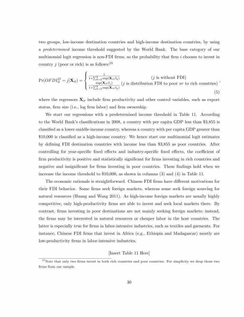
two groups, low-income destination countries and high-income destination countries, by using

a predetermined income threshold suggested by the World Bank. The base category of our

multinomial logit regression is non-FDI �rms, so the probability that �rm i chooses to invest in

country j (poor or rich) is as follows:23

Pr(OFDIDit = jjXit) =

8><>:1

1+P3k=2 exp(Xit�k)

exp(Xit�j)

1+P3k=2 exp(Xit�k)

(j is without FDI)(j is distribution FDI to poor or to rich countries)

;

(5)

where the regressors Xit include �rm productivity and other control variables, such as export

status, �rm size (i.e., log �rm labor) and �rm ownership.

We start our regressions with a predetermined income threshold in Table 11. According

to the World Bank�s classi�cations in 2008, a country with per capita GDP less than $3,855 is

classi�ed as a lower-middle-income country, whereas a country with per capita GDP greater than

$10,000 is classi�ed as a high-income country. We hence start our multinomial logit estimates

by de�ning FDI destination countries with income less than $3,855 as poor countries. After

controlling for year-speci�c �xed e¤ects and industry-speci�c �xed e¤ects, the coe¢ cient of

�rm productivity is positive and statistically signi�cant for �rms investing in rich countries and

negative and insigni�cant for �rms investing in poor countries. These �ndings hold when we

increase the income threshold to $10,000, as shown in columns (3) and (4) in Table 11.

The economic rationale is straightforward. Chinese FDI �rms have di¤erent motivations for

their FDI behavior. Some �rms seek foreign markets, whereas some seek foreign sourcing for

natural resources (Huang and Wang 2011). As high-income foreign markets are usually highly

competitive, only high-productivity �rms are able to invest and seek local markets there. By

contrast, �rms investing in poor destinations are not mainly seeking foreign markets; instead,

the �rms may be interested in natural resources or cheaper labor in the host countries. The

latter is especially true for �rms in labor-intensive industries, such as textiles and garments. For

instance, Chinese FDI �rms that invest in Africa (e.g., Ethiopia and Madagascar) mostly are

low-productivity �rms in labor-intensive industries.


23Note that only two �rms invest in both rich countries and poor countries. For simplicity we drop those two

�rms from our sample.

30

6.3 Threshold Estimates of the Linder Hypothesis

Beyond the conventional wisdom that FDI is determined by a proximity-concentration trade-

o¤, Fajgelbaum et al. (2011) argue that the per capita income of host countries is positively

correlated with market size. With trade costs, �rms are more likely to engage in FDI rather than

export when host markets are large (Markusen 1984). Thus, the standard Linder hypothesis,

which stresses that high-income countries have relatively large trade volume, applies to �rm FDI

behavior: high-income countries usually absorb more FDI. Our �nal exercise is to see whether

the Linder hypothesis for FDI works in China.

The �rst necessary step to perform this task is to classify destination country groups by

income. A common and simple way to do this is to use the World Bank�s classi�cation, as in

Table 10. However, this classi�cation su¤ers from two pitfalls. First, the threshold varies by

year. There are no clear and time-invariant cuto¤s for the income groups. Second, even if the

cuto¤s are �xed, the e¤ect of �rm productivity on �rm FDI may not exactly correspond to

the predetermined income cuto¤s. That is, host countries�per capita GDP is an endogenous

threshold for FDI �rms in response to productivity movement.

To overcome these empirical challenges, Hansen (1999, 2000) provides an econometric ap-

proach that considers endogenous threshold regressions. To motivate this, consider an empirical

speci�cation with a country�s per capita GDP (pcgdp) as a threshold variable:

�OFDIit = �Xit + �itOFDIit = �Xit + �it

if pcgdpit < T

if pcgdpit � T; (6)

where T is the threshold parameter to be estimated. OFDIit is �rm i�s FDI �ow in year t. Xit

refers to all regressors, including �rm productivity. Without loss of generality, �it is i.i.d with

normal distribution: �it~N(0; �2i ). By using an indicator function I(�), we can re-express Equ.(6) as:

OFDIit = �Xit � I(pcgdpit < T ) + �Xit � I(pcgdpit � T ) + �it:

As this is a nonlinear regression, we can use the nonlinear squares approach to minimize

the sum of squared residuals. Since the estimators also include the threshold parameter T̂ , the

most convenient computational method to obtain the linear squares estimate is via concentration.

Thus, the optimal threshold parameter T̂ is chosen to minimize the concentrated sum of squared

errors function so that T̂ = argmin SSR(�(T ); �(T ); T ). Based on this, Hansen (1999, 2000)

31

developed an asymptotic distribution theory for the threshold regression estimates.

Table 12 presents the threshold regression results. By comparison, we start from a regression

without considering the threshold e¤ect in columns (1) and (2). By abstracting away all other

variables, we see that �rm TFP is positively correlated to �rm log FDI �ow, as shown in column

(1). The speci�cation in column (2) yields similar results by controlling industry-speci�c �xed

e¤ects and year-speci�c �xed e¤ects. The threshold regression results are reported in columns

(3) and (4). The estimated threshold parameter of host countries�log per capita GDP is 10.73

(or equivalently, per capita GDP is $45,524). As before, the coe¢ cient of �rm productivity is

positive and statistically signi�cant for high-income FDI destinations. However, for low-income

host countries, where per capita GDP is lower than the estimated threshold, the e¤ect of �rm

productivity on �rm FDI �ow is statistically insigni�cant, suggesting that �rm productivity is

not a crucial determinant of �rm FDI �ow. This �nding is robust even when we control for

year-speci�c �xed e¤ects and industry-speci�c �xed e¤ects in columns (5) and (6), suggesting

that the Linder hypothesis for FDI volume to high-income destination countries holds but may

not exist for FDI volume to low-income countries. This result con�rms that Chinese �rms�

investment in poor countries may not be labeled as "horizontal" FDI: tari¤-jumping motivation

or seeking foreign markets may not be a top priority for these �rms (Kolstad and Wiig 2012).


7 Concluding Remarks

This paper is one of the �rst to explore how �rm heterogeneity in�uences the volume of Chinese

distribution FDI. The rich data set enabled us to examine not only the extensive margin, but

also the intensive margin of Chinese outward FDI.

We found that �rms with distribution FDI are more productive than non-FDI �rms, but less

productive than non-distribution FDI �rms. These �ndings re�ect the fact that many Chinese

exporters are insu¢ ciently productive to build up production lines in foreign markets. As a com-

promise, such �rms set up foreign distribution centers to promote their exports. We also found

that with higher cross-border communications costs (iceberg transport costs), there is a higher

probability that �rms engage in distribution (non-distribution) FDI. Finally, high-productivity

�rms invest more in high-income countries but not necessarily in low-income countries.

32

References[1] Acemoglu, Daron and Jörn-Ste¤en Pischke (1998), "Why do Firms Train? Theory and

Evidence," Quarterly Journal of Economics, pp.79-119.

[2] Ahn, JaeBin, Amit Khandelwal, and Shang-jin Wei (2010), "The Role of Intermediaries inFacilitating Trade," Journal of International Economics 84(1), pp. 73-85.

[3] Amiti, Mary and Donald Davis (2011), "Trade, Firms, and Wages: Theory and Evidence,"Review of Economic Studies 79, pp. 1-36.

[4] Amiti, Mary, and Jozef Konings (2007), "Trade Liberalization, Intermediate Inputs, andProductivity: Evidence from Indonesia," American Economic Review 97(5), pp. 1611-1638.

[5] Antràs, Pol and Elhanan, Helpman (2004), "Global Sourcing," Journal of Political Economy112, pp. 552-580.

[6] Arkolakis, Costas and Marc-Andreas Muendler (2011), "The Extensive Margin of ExportingProducts: A Firm-level Analysis," mimeo, Yale University.

[7] Berman, Nicolas, Philippe Martin and Thierry Mayer, (2012), �How Do Di¤erent ExportersReact to Exchange Rate Changes?�Quarterly Journal of Economics, 127, pp. 437-492.

[8] Bhattacharya Rudrani, Ila Patnaik, and Ajay Shah (2010), "Productivity and OutboundFDI in Software Services: a Reversal of the HMYModel," working paper, National Instituteof Public Finance and Policy, New Delhi.

[9] Blonigen, Bruce (2001), "In Search of Substitution between Foreign Production and Ex-ports," Journal of International Economics 53(1), pp. 81-104.

[10] Blonigen, Bruce (2005), �A Review of the Empirical Literature on FDI Determinants,�Atlantic Economic Journal 33, pp. 383�403.

[11] Boatman, Kara (2007), �What Determines Distribution FDI?� Journal of Business andPublic A¤airs, 1(1).

[12] Brandt, Loren, Johannes Van Biesebroeck, and Yifan Zhang (2012), "Creative Account-ing or Creative Destruction? Firm-level Productivity Growth in Chinese Manufacturing?"Journal of Development Economics, 97, pp. 339-351.

[13] Cameron, Colin and Pravin Trivedi (2005), Microeconometrics: Methods and Applications,Cambridge University Press.

[14] Chen, Qiang (2014), "Climate Shocks, State Capacity, and Peasant Uprisings in NorthChina during 25-1911 CE.," Economica, forthcoming.

[15] Chen, Wenjie and Heiwai Tang (2014), "The Dragon is Flying West: Micro-Level Evidenceof Chinese Direct Investment," Asian Development Review 31(2), pp. 109-140.

[16] Conconi, Paola, André Sapir, and Maurizio Zanardi (2014), "The InternationalizationProcess of Firms: from Exports to FDI", mimeo, Lancaster University Management School.

[17] Dai, Mi, Madhura Maitra, and Miaojie Yu (2012), �Unexceptional Exporter Performancein China? The Role of Processing Trade,�mimeo, Peking University.

33

[18] Damijan, Joze P, Saso Polanec and Janez Prasnikar (2007), "FDI and Productivity: Micro-evidence from Slovenia," The World Economy, 30 (1), pp. 135�155.

[19] De Loecker, Jan (2011), "Product Di¤erentiation, Multiproduct Firms, and Estimating theImpact of Trade Liberalization on Productivity," Econometrica, 79(5), pp. 1407�1451.

[20] Eaton Jonathan, Samuel Kortum, and Francis Kramarz (2011), "An Anatomy of Interna-tional Trade: Evidence from French Firms," Econometrica 79(5), pp. 1453-1498.

[21] Fajgelbaum Pablo, Gene Grossman, and Elhanan Helpman (forthcoming), "A Linder Hy-pothesis for Foreign Direct Investment," Review of Economic Studies.

[22] Federico, Stefano (2009), "Outsourcing versus Integration at Home and Abroad," workingpaper, Bank of Italy.

[23] Feenstra, Robert and Gordon Hanson (2005),"Ownership and Control in Outsourcing toChina: Estimating the Property-Rights Theory of the Firm," Quarterly Journal of Eco-nomics 120(2), pp. 729-762.

[24] Feenstra, Robert, Zhiyuan Li, and Miaojie Yu (2014), "Exports and Credit Constraintsunder Incomplete Information: Theory and Evidence from China," Review of Economicsand Statistics, 96(4), pp.729-744.

[25] Froot, Kenneth and Jeremy Stein (1991), "Exchange Rates and Foreign Direct Investment:An Imperfect Capital Markets Approach", Quarterly Journal of Economics, pp.1191-1217.

[26] Groizard, Luis, Priya Ranjan, Antonio Rodriguez-Lopez (2015), "Trade Costs and JobFlows: Evidence from Establishment-Level Data," Economic Inquiry 53(1), pp. 173-204.

[27] Goldberg, Pinelopi, Amit Khandelwal, Nina Pavcnik, and Petia Topalova (2010), "ImportedIntermediate Inputs and Domestic Product Growth: Evidence from India," Quarterly Jour-nal of Economics 125 (4), pp. 1727-1767.

[28] Hansen, Bruce (1999), "Threshold e¤ects in non-dynamic panels: Estimation, testing andinference," Journal of Econometrics 93, 345-368.

[29] Hansen, Bruce (2000), "Sample Splitting and Threshold Estimation," Econometrica 68(3),pp. 575-603.

[30] Hanson, Gordon H., Mataloni, Raymond J., Slaughter, Mathhew J. (2001), �ExpansionStrategies of U.S. Multinational Firms,� National Bureau of Economic Research (Cam-bridge, MA) Working Paper No. 8433.

[31] Head, Keith and John Ries (2003), "Heterogeneity and the FDI versus Export Decisionof Japanese Manufacturers," Journal of the Japanese International Economies 17(4), pp.448�67.

[32] Halpern, Laszlo, Miklos Koren, and Adam Szeidl (2010), "Imported Inputs and Productiv-ity," University of California, Berkeley, Mimeo.

[33] Helpman, Elhanan, Marc J. Melitz and Steven R. Yeaple (2004), "Export vs. FDI," Amer-ican Economic Review 94(1), pp. 300�16.

34

[34] Horstmann, Ignatius J. and James R. Markusen (1996), �Exploring New Markets: DirectInvestment, Contractual Relations and the Multinational Enterprise,� International Eco-nomic Review, 37(1), pp. 1-19.

[35] Hsieh, Chang-Tai and Peter Klenow (2009), "Misallocation and Manufacturing TFP inChina and India," Quarterly Journal of Economics 124(4), pp. 1403-48.

[36] Huang, Yiping and Bijun Wang (2011), �Chinese Direct Investment: Is There a ChinaModel?�China & World Economy 19(4), pp. 1-21.

[37] Imbens, Guido (2004), "Nonparametric Estimation of Average Treatment E¤ects UnderExogeneity: A Review," Review of Economics and Statistics 86(1), pp. 4-29.

[38] Ishikawa, Jota, Hodaka Morita, and Hiroshi Mukunnoki (2010), �FDI in Post-ProductionServices and Product Market Competition,�Journal of International Economics 82(1), pp.73-84.

[39] Ishikawa, Jota and Hodaka Morita (2015), �Trade Liberalization and Aftermarket Servicesfor Imports,�mimeo, Hitotsubashi University.

[40] Jovanovic, Boyan J.(1982), "Selection and the Evolution of Industry," Econometrica 50,pp. 649-670.

[41] Kimura, Fuku and Hyun-Hoon Lee (2006), "The Gravity Equation in International Tradein Services," Review of International Economics, 142(1), pp 92-121.

[42] King, Gary and Langche Zeng (2001), "Logistic Regression in Rare Events Data," PoliticalAnalysis 9(2), pp. 137-163.

[43] King, Gary and Langche Zeng (2002), "Estimating Absolute, Relative, and AttributableRisks in Case-Control Studies," Statistics in Medicine 21, pp. 1409-1427.

[44] Kolstad Ivar and Arne Wilg (2012), "What determines Chinese FDI?" Journal of WorldBusiness, 47(1), pp. 26-34.

[45] Levinsohn, James and Amil Petrin (2003), "Estimating Production Functions Using Inputsto Control for Unobservable," Review of Economic Studies 70(2), pp. 317-341.

[46] Linder, Sta¤en Burenstam (1961), An Essay on Trade and Transformation, Stockholm:Almqvist and Wiksell.

[47] Lu Dan (2010), "Exceptional Exporter Performance? Evidence from Chinese Manufactur-ing Firms," mimeo, University of Chicago.

[48] Markusen, James R. (1984), "Multinationals, Multi-Plant Economies, and the Gains fromTrade," Journal of International Economics 16 (3-4), pp. 205-26.

[49] Melitz, Marc (2003), "The Impact of Trade on Intra-industry Reallocations and AggregateIndustry Productivity," Econometrica 71(6), pp. 1695�725.

[50] Nunn, Nathan (2007), "Relationship-speci�city, Incomplete Contracts, and the Pattern ofTrade," Quarterly Journal of Economics, May 2007, pp. 569-600.

[51] Oldenski, Lindsay (2012), "Export Versus FDI and the Communication of Complex Infor-mation,"Journal of International Economics 87, 312-322.

35

[52] Olley, Steven and Ariel Pakes (1996), "The Dynamics of Productivity in the Telecommu-nications Equipment Industry," Econometrica 64(6), pp. 1263-1297.

[53] Qiu, Larry, D. and Ying Xue (2014), "Understanding China�s Foreign Trade: a LiteratureReview (I)," China Economic Journal, 7(2), pp. 168-186.

[54] Ramondo, Natalia, Veronica Rapporport, Kim J. Ruhl (2014), "The Proximity-Concentration Tradeo¤ under Uncertainty," Review of Economic Studies, forthcoming.

[55] Russ, Katheryn N.(2007), "The Endogeneity of the Exchange Rate as a Determinant of FDI:A Model of Money, Entry, and Multinational Firms," Journal of International Economics71(2), pp. 344-372.

[56] Wang, Bijun, Yuyan Tan, Miaojie Yu, and Yiping Huang (2015), " Direct Investment, FirmProductivity, and Credit Constraints: Evidence from Chinese Firms," Paci�c EconomicReview, forthcoming.

[57] Wang, Chengqi, Junjie Hong, Mario Kafouros, Agyenim Boateng (2012), "What DrivesFDI of Chinese Firms? Testing the Explanatory Power of Three Theoretical Frameworks,"International Business Review, 21(3). pp. 425-438.

[58] Yeaple, Stephen (2005), �A Simple Model of Firm Heterogeneity, International Trade, andWages,�Journal of International Economics 65(1), pp.1-20.

[59] Yu, Miaojie (2015), "Processing Trade, Tari¤Reductions, and Firm Productivity: Evidencefrom Chinese Firms," Economic Journal, 125 (June), pp. 943�988.

36

Table1:FDIShareinNumberofManufacturingFirms(2000-08)

Firmtype

2000

2001

2002

2003

2004

2005

2006

2007

2008

NationwideFDIdecisiondata

(1)Mfg.�rms

84,974

100,091

110,522

129,720

200,989

198,285

248,601

258,246

222,312

(2)FDIstarting�rms

197

340

444

587

972

984

1,081

1,140

1,018

(3)FDImfg.�rms

1417

2030

103

431

761

1,168

1,183

(4)DistributionFDImfg.�rms2

23

440

224

407

616

656

(5)FDIshare(%)

0.23

0.34

0.40

0.45

0.48

0.49

0.43

0.44

0.46

(6)DistributionFDIshare(%)

14.2

11.7

15.0

13.3

38.8

51.9

53.5

52.7

55.4

Zhejiang�sFDI�owdata

(7)Mfg.�rms

35,887

39,465

27,433

(8)FDI�rms

424

419

427

(9)FDImfg.Firms

113

163

131

(10)FDIshare(%)

0.31

0.41

0.48

Note:Dataarefrom

theMinistryofCommerceofChina

andtheauthors�calculations.FDIshare(%=(2)/(1))isobtainedby

dividing

the

numberofFDIstarting�rmsbythenumberofmanufacturing�rmsnationwideandinZhejiangprovince,respectively.DistributionFDIshare

(=(4)/(3))isobtainedbydividingthenumberofdistributionFDImanufacturing�rmsbythenumberoftotalFDImanufacturing�rms.For

Zhejiang�rms,theFDIdecisiondataareavailableeveryyearduringthesample,buttheFDI�owdataareavailableonlyfor2006-08,forwhich

thereare1,270FDI�rmsinZhejiangand407ofthem

aremanufacturing�rms.

37

Table 2: Summary Statistics of Key VariablesSample Covered: Nationwide (2000-08) Zhejiang (2006-08)Variable Mean Std. dev. Mean Std. dev.Firm log FDI 3.27 1.53Firm FDI indicator 0.004 0.066 0.003 0.05Firm TFP (Olley-Pakes) 3.61 1.18 4.08 0.94Firm export indicator 0.29 0.451 0.42 0.49SOE indicator 0.05 0.219 0.002 0.047Foreign indicator 0.20 0.402 0.16 0.366Firm log labor 4.78 1.115 4.45 0.983

38

Table3:Di¤erencebetweenNon-FDIandFDIFirms

Category

#ofobs.

Mean

Variable

TFP

LogEmployees

Sales

Export

PropensityScoreMatching

Unmatched

Matched

(1)

(2)

(3)

(4)

(5)

(6)

FDIFirmsvs.Non-FDIFirms

(i)Non-FDI�rms

1,137,097

3.604

3.811

4.742

96,560

18,615

(ii)FDI�rms

3,727

4.289

4.289

5.844

3,334,672

1,285,675

Di¤erence=(ii)-(i)

0.685***

0.478***

1.102***

3,238,112***

1,267,060***

(35.41)

(9.54)

(61.34)

(150.3)

(120.1)

(iii)DistributionFDI�rms

1,954

4.180

4.180

5.604

1,245,375

460,793

Di¤erence=(iii)-(i)

0.576***

0.442***

0.862***

1,148,815***

442,178***

(21.55)

(8.44)

(34.83)

(50.37)

(39.22)

(iv)Non-DistributionFDI�rms1,773

4.411

4.411

6.109

5,637,258

2,194,766

Di¤erence=(iii)-(iv)

-0.231***

-0.086

-0.505***

-4,391,884***

-1,733,972***

(-5.73)

(-1.39)

(-8.45)

(-9.19)

(-7.63)

Note:Numbersinparenthesesaret-values.***denotessigni�canceatthe1%

level.Columns(2)and(3)reporttheTFPcomparisonbyusing

thenearest-matchingpropensityscorematching(PSM

)approach.Column(2)isunmatchedwhereascolumn(3)istheaveragetreatmentonthe

treated(ATT)approach.ThetreatedgroupisFDI�rms,whereasthecontrolgroupisnon-FDI�rms.Firmsize(inloglabor),exports,and

salesareusedascovariatestoobtainthepropensityscore.Sincethereareobservationswithidenticalpropensityscorevalues,thesortorderof

thedatacoulda¤ecttheresults.Thesortorderismadetoberandom

beforeadoptingthePSM

approach.

39

Table4:TFPDi¤erencebetweenDistributionFDIFirmsandotherFirmsbyYear

FirmTFP

2000

2001

2002

2003

2004

2005

2006

2007

2008

(1)Non-FDIFirms

3.109

3.001

3.218

3.283

3.065

3.421

3.540

3.659

4.966

(2)AllFDIFirms

4.396

4.190

4.376

5.309

4.163

3.855

3.738

3.738

5.194

(3)DistributionFDIFirms

5.514

5.564

5.888

4.514

3.855

3.634

3.578

3.744

5.150

(4)Non-DistributionFDIFirms

4.210

4.007

4.109

5.432

4.358

4.093

3.923

4.026

5.248

TFPDi¤erence=(3)-(1)

2.404***

2.562***

2.670***

1.231***

0.790***

0.213***

0.038

0.085**

0.184***

(3.23)

(3.49)

(4.50)

(2.43)

(4.56)

(3.09)

(0.73)

(2.01)

(5.14)

TFPDi¤erence=(3)-(4)

1.304***

1.557***

1.778***

-0.917

-0.502***

-0.458***

-0.344***

-0.282***

-0.098*

(2.03)

(2.75)

(3.55)

(-1.44)

(-1.90)

(-4.34)

(-4.45)

(-4.35)

(-1.79)

NumberofObservations

39,337

46,957

51,760

105,348

151,546

170,635

193,644

220,517

157,353

Note:Numbersinparenthesesaret-values.***(**,*)denotessigni�canceatthe1%

(5%,10%)level.Thetablereports�rmTFPdi¤erence

betweendistributionFDIandnon-distributionFDI�rmsand�rmTFPdi¤erencebetweendistributionFDIandnon-FDI�rms.

40

Table5:E¤ectsofFirmProductivityonFDIDecision(2000-08)

Regressand:Indicatorof

FDIStarter

EverFDI

EconometricMethod:

LPM

Probit

Logit

RareEvent

Complementary

Logit

Logit

Logit

Logit

Log-Log

Variable:

(1)

(2)

(3)

(4)

(5)

(6)

(7)

(8)

FirmRelativeTFP

0.001***

0.321***

1.076***

1.086***

1.084***

1.079***

0.988***

0.893***

(4.54)

(5.11)

(5.62)

(5.68)

(5.61)

(4.66)

(5.11)

(7.69)

SOEIndicator

-0.001***

-0.310***

-0.874***

-0.876***

-0.878***

-0.963***

�-0.613***

(-3.91)

(-5.17)

(-4.95)

(-4.96)

(-4.85)

(-5.43)

(-5.96)

ForeignIndicator

-0.001***

-0.183***

-0.577***

-0.575***

-0.573***

�-0.578***

-0.704***

(-5.26)

(-7.77)

(-8.18)

(-8.16)

(-8.76)

(-8.18)

(-15.55)

LogFirmLabor

0.001***

0.208***

0.615***

0.614***

0.610***

0.642***

0.605***

0.577***

(15.59)

(26.18)

(28.33)

(28.30)

(29.31)

(25.56)

(27.13)

(42.90)

ExportIndicator

0.002***

0.431***

1.373***

1.373***

1.372***

1.460***

1.370***

1.096***

(15.27)

(19.91)

(19.64)

(19.63)

(20.46)

(19.19)

(19.40)

(27.60)

SOEDropped

No

No

No

No

No

No

Yes

No

ForeignFirmsDropped

No

No

No

No

No

Yes

No

No

YearFixedE¤ects

Yes

Yes

Yes

Yes

Yes

Yes

Yes

Yes

IndustryFixedE¤ects

Yes

Yes

Yes

Yes

Yes

Yes

Yes

Yes


1,138,450

1,137,309

1,137,309

1,138,450

1,138,450

896,958

1,097,537

1,139,683

Note:Theregressand

istheFDIindicator.Numbersinparenthesesaret-values.***denotessigni�canceatthe1%

level.Column(6)drops

foreign�rmsfrom

thesamplewhereascolumn(7)dropsSOEsfrom

thesample.

41

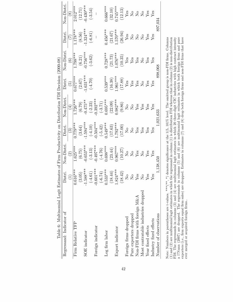
Table6:MultinomialLogitEstimatesofFirmProductivityonDistributionFDIDecision(2000-08)


Distri.

Non-Distri.

Distri.

Non-Distri.

Distri.

Non-Distri.

Distri.

Non-Distri.

(1)

(2)

(3)

(4)

(5)

(6)

(7)

(8)

FirmRelativeTFP

0.616***

1.625***

0.779***

1.726***

0.677***

1.798***

1.178***

2.012***

(3.05)

(6.75)

(3.64)

(6.79)

(2.67)

(6.21)

(8.56)

(12.71)

SOEindicator

-1.588***

-0.653***

-1.594***

-0.475**

-1.631***

-0.756***

-1.324***

-0.430***

(-4.61)

(-3.13)

(-4.10)

(-2.23)

(-4.70)

(-3.62)

(-6.81)

(-3.54)

Foreignindicator

-0.601***

-0.497***

-0.504***

-0.392***

��

(-6.74)

(-4.76)

(-5.42)

(-3.71)

Log�rmlabor

0.533***

0.698***

0.549***

0.695***

0.539***

0.728***

0.456***

0.666***

(18.44)

(23.44)

(17.63)

(22.09)

(16.38)

(21.73)

(21.67)

(32.10)

Exportindicator

1.824***

0.967***

1.792***

0.982***

1.961***

1.076***

1.570***

0.745***

(18.42)

(10.27)

(17.00)

(9.86)

(17.88)

(10.35)

(26.94)

(12.13)

Foreign�rmsdropped

No

No

No

No

Yes

Yes

Yes

Yes

Pureexportersdropped

No

No

No

No

Yes

Yes

No

No

Non-FDI�rmswithforeignM&A

Yes

Yes

Yes

Yes

Yes

Yes

No

No

Mostcontratableindustriesdropped

No

No

Yes

Yes

No

No

No

No

Year�xede¤ects

Yes

Yes

Yes

Yes

Yes

Yes

Yes

Yes

Industry�xede¤ects

Yes

Yes

Yes

Yes

Yes

Yes

Yes

Yes

Numberofobservations

1,138,450

1,021,633

898,068

897,034

Note:Numbersinparenthesesaret-values.***(**,*)denotessigni�canceatthe1(5,10)%

level.Theomittedgroupisnon-FDI�rms.Columns

(1)and(2)aremultinomiallogitestimatesinwhichtheregressandincolumn(1)isdistributionFDIwhereasthatincolumn(2)isnon-distribution

FDI.Theregressandsincolumns(3)and(4)aremultinomiallogitestimatesinwhich20three-digitCICindustrieswithhighcontractintensity

al?Nunn(2007)aredropped.Theregressandsincolumns(5)and(6)aremultinomiallogitestimatesinwhichbothforeign�rmsandpure

exporters(i.e.,�rmexportsequal�rmsales)aredropped.Estimatesincolumns(7)and(8)dropbothforeign�rmsandnon-FDI�rmsthathave

evermergedoracquiredforeign�rms..

42

Table 7: IV Estimates of Firm Productivity on FDI Decision (2005-08)Econometric method: Probit Rare events Multinomial Logit

LogitRegressand: FDI Indicator for All FDI All FDI Distribution Non-Distribution

(1) (2) (3) (4)Firm TFP 0.854*** 4.575*** 1.376*** 1.487***

(31.24) (7.40) (3.54) (3.62)SOE Indicator 0.149*** 0.799*** -0.969*** 0.160

(3.43) (2.80) (-2.41) (0.62)Foreign Indicator -0.091*** -0.524*** -0.720*** -0.467***

(-5.33) (-6.34) (-6.73) (-3.83)Log Firm Labor 0.094*** 0.532*** 0.510*** 0.685***

(8.31) (18.40) (14.89) (17.52)Export Indicator 0.260*** 1.562*** 1.858*** 1.021***

(10.89) (18.92) (15.84) (9.07)Year-speci�c Fixed E¤ects Yes Yes Yes YesIndustry-speci�c Fixed E¤ects Yes Yes Yes YesNumber of Observations 484,212 484,212 484,212 484,212

First-Stage RegressionIV: Log Firm Training Expenses 0.028***

(30.40)

Notes: The regressands in columns (1), (2), and (5) are the FDI indicator whereas those in columns (3) and(6) are the distribution FDI indicator and those in columns (4) and (7) are the non-distribution FDI indicator.Numbers in parenthesis are bootstrapped t-values. ***(**) denotes signi�cance at the 1(5)% level. The estimatesin column (1) are probit IV estimates, whereas those in columns (2) and (5) are IV rare-events logit estimates.Columns (3)-(4) are IV multinomial logit estimates. The omitted group is non-FDI �rms. The instrument is theone-year lag of �rm�s log training expenses from the period 2005 to 2008.

43

Table 8: Advertising Expenses by Di¤erent Types of Firms (2004-07)Regressand: Log Firm Advertising Expenses (1) (2) (3) (4)Non FDI Indicator -1.32*** -0.56*** -0.62*** -0.77***

(-8.33) (-5.53) (-4.27) (-5.23)Non-Distribution FDI Indicator 0.57** 0.32** 0.32 0.22

(2.33) (2.14) (1.38) (0.97)SOE Indicator -0.54*** -0.53*** -0.56***

(-19.13) (-13.69) (-14.52)Foreign Indicator 0.22*** � �

(16.32)Log Firm Labor 0.70*** 0.69*** 0.72***

(138.07) (88.20) (92.69)Export Indicator -0.02 0.08***

(-1.58) (4.75)Export Share � 2-digit Industry Fixed E¤ects No No No YesYear Fixed E¤ects Yes Yes Yes Yes2-digit Industry Fixed E¤ects Yes Yes Yes YesNumber of Observations 128,028 128,026 99,679 98,424R-squared 0.06 0.22 0.23 0.23

Notes: The regressand is �rm log advertising expenses. Numbers in parentheses are t-values clustered at the�rm level. ***(**,*) denotes signi�cance at the 1(5, 10)% level. The omitted group is distribution FDI �rms.Columns (3) and (4) drop foreign �rms from the sample. Column (4) includes the interaction terms betweenexport intensity (i.e., �rm exports over �rm total sales) with two-digit industry �xed e¤ects.

44

Table9:IntensiveEstimatesofDistributionFDIvsTotalFDIFlowforZhejiangFirms(2006-08)

EconometricMethod:

OLS

Heckman

1st -step

2nd-step

1st-step

2nd-step

Regressand:

LogFDIof

LogFDIof

Dist.FDILogDist.

FDI

Log

LogDist.

AllFDIFirms

Dist.FDIFirms

Dummy

FDI

Dummy

FDI

FDI

(1)

(2)

(3)

(4)

(5)

(6)

(7)

(8)

(9)

FirmRelativeTFP

0.922*

0.866*

(1.92)

(1.88)

FirmTFP

0.204*

0.193*

0.720***

4.968***

0.703***

3.429*

4.751***

(1.90)

(1.88)

(4.01)

(2.66)

(4.12)

(1.92)

(2.86)

SOEIndicator

2.492***

2.488***

2.689***

-0.329

1.141

(7.09)

(7.08)

(7.77)

(-0.85)

(1.40)

ForeignIndicator

0.081

0.080

0.097

0.097

-0.185***

-1.158**

-0.150***

-0.643

-0.880**

(0.39)

(0.39)

(0.46)

(0.46)

(-3.06)

(-2.15)

(-2.69)

(-1.40)

(-2.00)

LogFirmLabor

0.314***

0.315***

0.339***

0.340***

0.133**

1.162***

0.149**

0.986***

1.294***

(4.03)

(4.04)

(4.53)

(4.54)

(2.03)

(3.44)

(2.35)

(2.61)

(3.58)

ExportIndicator

-0.603**

-0.600**

-0.647**

-0.647**

0.527***

2.987**

0.502***

1.754

2.645**

(-2.04)

(-2.03)

(-2.05)

(-2.05)

(5.45)

(2.10)

(5.71)

(1.33)

(2.15)

FirmTenure

0.002

0.003

(0.39)

(1.00)

Inversermillsratio

7.506**

5.207*

7.372***

(2.58)

(1.82)

(2.79)

YearFixedE¤ects

Yes

Yes

Yes

Yes

Yes

Yes

Yes


Yes

Yes

Yes

Yes

Yes

Yes

Yes


251

251

210

210

60198

251

60,358

251

210

R-squared

0.13

0.13

0.15

0.15

�0.16

�0.15

0.18

.First-stageEstimates

IV:LogFirmTraining

��

��

0.049***

�0.011***

��

(21.86)

(22.29)

Note:Numbersinparenthesesare(bootstrapped)t-values.***(**,*)denotessigni�canceatthe1%

(5%,10%)level.TheregressandintheOLS

estimatesincolumns(1)-(2)aretotalFDI�owwhereasthoseincolumns(3)-(4)aredistributionFDI�ow.Therestofthetableisthethree-step

HeckmanIV

estimates:(i)The�rststageregresses�rmTFPontheone-yearlagof�rm�slogtrainingexpenses.(ii)Thesecond

stageisthe

probitestimates,whichregressthe�rmdistributionFDIindicatoronthe�ttedvariablesofTFPobtainedfrom

(i).Firmtenureservesasthe

exclusivevariable,whichisonlyincludedinthesecond-stagebutnotinthethird-stage.(iii)Thethird-stageestimatesincolumn(6)regress

logdistributionFDIon�ttedTFPandothercontrolvariables.TheinverseMillsratiocalculatedfrom

thesecond-stageisinsertedinthethird

stageasanadditionalregressor.Theestimatesincolumns(7)-(9)aresimilartotheestimatesincolumns(5)and(6)excepttheregressand

of

thesecondstageis�rmtheFDIindicatorandthatofthethirdstageis�rm�slogFDI�owincolumn(8)and�rm�slogdistributionFDI�owin

column(9).

45

Table10:MultinomialLogitEstimatesbyHostInvestmentEnvironment(2006-2008)


Dist.

Non-Dist.

Dist.

Non-Dist.

Dist.

Non-Dist.

(1)

(2)

(3)

(4)

(5)

(6)

FirmRelativeTFP

3.41***

4.84**

3.41***

4.84**

4.24***

4.38*

(3.17)

(2.08)

(3.17)

(2.08)

(3.02)

(1.94)

DaysofImportDocumentPreparation

0.26*

-0.19

0.26*

0.03

0.30*

0.05

(1.76)

(-0.83)

(1.70)

(0.12)

(1.65)

(0.20)

ImportTari¤s

0.08

0.13**

0.07

0.17**

0.04

0.17*

(1.51)

(2.04)

(1.43)

(2.18)

(0.66)

(1.95)

SOEIndicator

-10.85***

3.22***

-14.92***

2.82**

-10.86***

3.21***

(-72.12)

(3.00)

(-75.15)

(2.44)

(-68.68)

(2.94)

ForeignIndicator

0.60**

0.43

0.52*

0.39

��

(2.24)

(0.74)

(1.94)

(0.66)

Logper-capitaGDP

0.97***

0.33

0.97***

0.65

0.81**

0.60

(3.36)

(0.92)

(3.37)

(1.56)

(2.48)

(1.19)

ForeignFirmsDropped

No

No

No

No

Yes

Yes

LogBilateralDistancecontrolled

Yes

Yes

Yes

Yes

Yes

Yes

Year-speci�cFixedE¤ects

Yes

Yes

Yes

Yes

Yes

Yes

YearDummy�LogBilateralDistance

No

No

Yes

Yes

Yes

Yes

Industry-speci�cFixedE¤ects

Yes

Yes

Yes

Yes

Yes

Yes


1,999,441

1,999,441

1,679,207

Note:Numbersinparenthesesare(bootstrapped)t-values.***(**,*)denotessigni�canceatthe1%

(5%,10%)level.Theregressandsincolumns

(1),(3),and(5)aretheindicatorofdistributionFDI,whereasthoseincolumns(2),(4),and(6)aretheindicatorofnon-distributionFDI.The

omittedgroupisnon-FDI�rms.

46

Table11:MultinomialLogitEstimatesoftheDistributionFDIDecisionbyDestinationIncome(2006-08)

Predeterminedincomethreshold

GDPPC=$3,885

GDPPC=$10,000

Regressand:DistributionFDIdecision

Dist.FDItopoorDist.FDItorich

Dist.FDItopoorDist.FDItorich

(1)

(2)

(3)

(4)

FirmRelativeTFP

0.058

1.371***

0.377

1.420***

(0.04)

(3.06)

(0.36)

(3.03)

Logoflabor

0.500***

0.656***

0.668***

0.637***

(3.05)

(10.44)

(5.49)

(9.46)

Exportindicator

1.569***

2.302***

1.974***

2.254***

(3.05)

(8.47)

(4.28)

(8.00)

SOEindicator

-15.33***

-15.67***

-17.70***

-17.44***

(-25.21)

(-55.99)

(-35.42)

(-61.60)

Foreignindicator

-0.773

-0.177

-1.016**

-0.086

(-1.25)

(-1.04)

(-2.12)

(-0.49)

Year-speci�c�xede¤ects

Yes

Yes

Yes

Yes

Industry-speci�c�xede¤ects

Yes

Yes

Yes

Yes


100,806

100,806

Note:TheregressandisthedistributionFDIindicatorinwhichzerodenotesnotanytypeofFDI,onereferstodistributionFDItopoorcountries,

andtwodenotesdistributionFDItorichcountries.Numbersinparenthesesaret-values.***(**)denotessigni�canceatthe1%

(5%)level.The

sampleinthistablecoversZhejiangmanufacturing�rmsduring2006-08.Two-digitChineseindustryclassi�cationindustry-speci�c�xede¤ects

areincludedinalltheestimations.

47

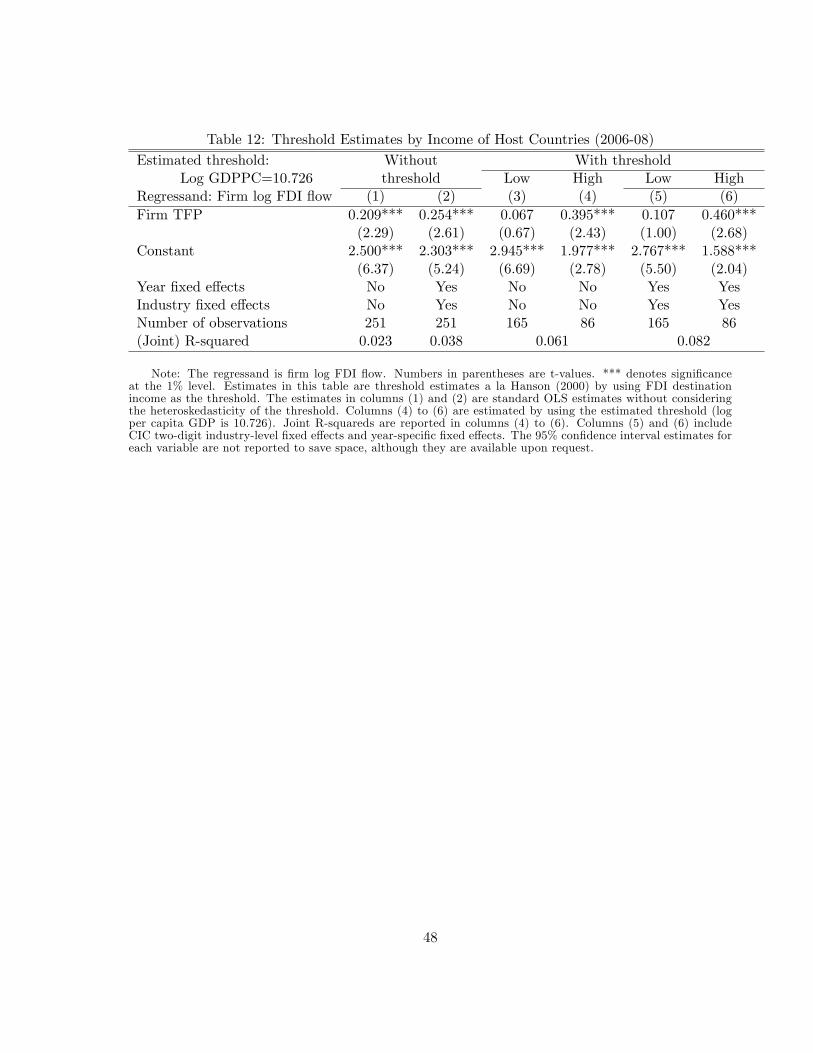
Table 12: Threshold Estimates by Income of Host Countries (2006-08)Estimated threshold: Without With threshold

Log GDPPC=10.726 threshold Low High Low HighRegressand: Firm log FDI �ow (1) (2) (3) (4) (5) (6)Firm TFP 0.209*** 0.254*** 0.067 0.395*** 0.107 0.460***

(2.29) (2.61) (0.67) (2.43) (1.00) (2.68)Constant 2.500*** 2.303*** 2.945*** 1.977*** 2.767*** 1.588***

(6.37) (5.24) (6.69) (2.78) (5.50) (2.04)Year �xed e¤ects No Yes No No Yes YesIndustry �xed e¤ects No Yes No No Yes YesNumber of observations 251 251 165 86 165 86(Joint) R-squared 0.023 0.038 0.061 0.082

Note: The regressand is �rm log FDI �ow. Numbers in parentheses are t-values. *** denotes signi�canceat the 1% level. Estimates in this table are threshold estimates a la Hanson (2000) by using FDI destinationincome as the threshold. The estimates in columns (1) and (2) are standard OLS estimates without consideringthe heteroskedasticity of the threshold. Columns (4) to (6) are estimated by using the estimated threshold (logper capita GDP is 10.726). Joint R-squareds are reported in columns (4) to (6). Columns (5) and (6) includeCIC two-digit industry-level �xed e¤ects and year-speci�c �xed e¤ects. The 95% con�dence interval estimates foreach variable are not reported to save space, although they are available upon request.

48

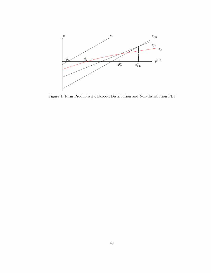
Figure 1: Firm Productivity, Export, Distribution and Non-distribution FDI

49

0.1

.2.3

.4K

erna

l Den

sity

of L

og T

FP

5 0 5 10 15x

Non OFDI firmDistribution OFDI firmOther OFDI firm

Figure 2: Firm Productivity by Firm Type

50

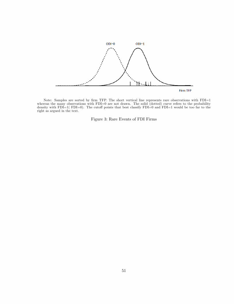
Note: Samples are sorted by �rm TFP. The short vertical line represents rare observations with FDI=1whereas the many observations with FDI=0 are not drawn. The solid (dotted) curve refers to the probabilitydensity with FDI=1( FDI=0). The cuto¤ points that best classify FDI=0 and FDI=1 would be too far to theright as argued in the text.

Figure 3: Rare Events of FDI Firms

51

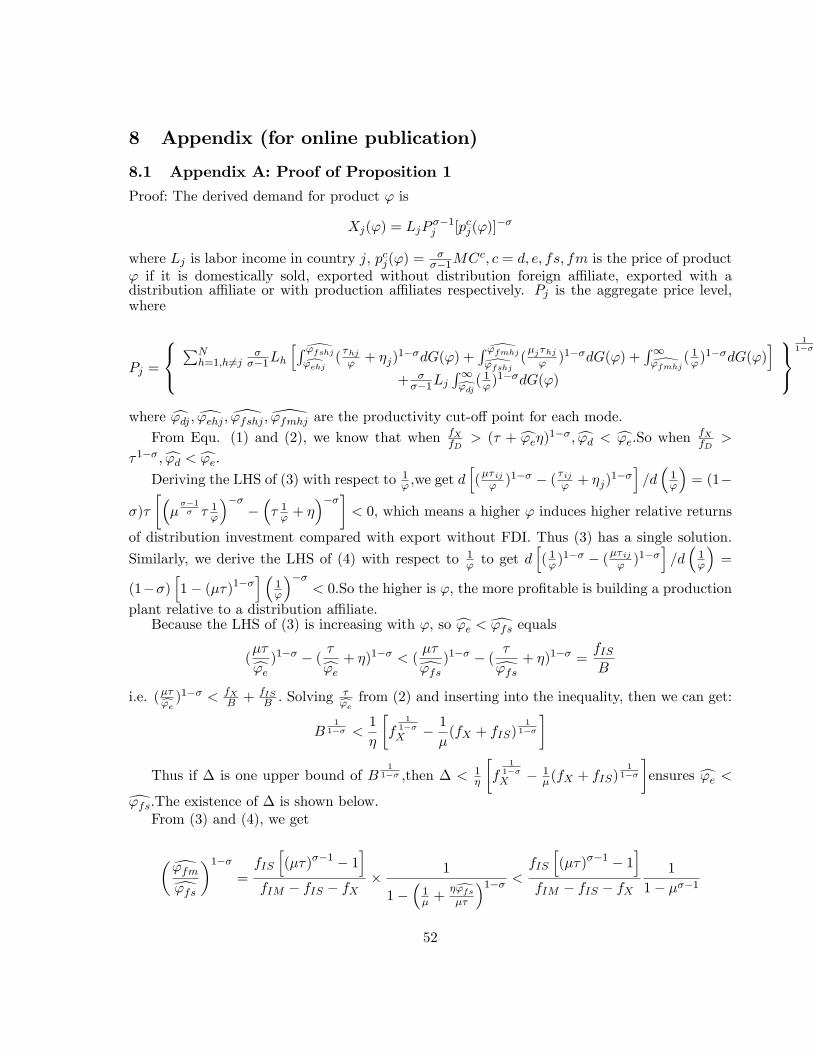
8 Appendix (for online publication)

8.1 Appendix A: Proof of Proposition 1Proof: The derived demand for product ' is

Xj(') = LjP��1j [pcj(')]

��

where Lj is labor income in country j, pcj(') =��1MC

c; c = d; e; fs; fm is the price of product' if it is domestically sold, exported without distribution foreign a¢ liate, exported with adistribution a¢ liate or with production a¢ liates respectively. Pj is the aggregate price level,where

Pj =

8<:PNh=1;h 6=j

��1Lh

hR\'fshjd'ehj ( �hj' + �j)1��dG(') +

R \'fmhj\'fshj

(�j�hj' )1��dG(') +

R1\'fmhj

( 1')1��dG(')

i+ ��1Lj

R1d'dj ( 1')1��dG(')9=;

11��

where c'dj ; d'ehj ; ['fshj ;\'fmhj are the productivity cut-o¤ point for each mode.From Equ. (1) and (2), we know that when fX

fD> (� + c'e�)1��;c'd < c'e:So when fX

fD>

�1��;c'd < c'e:Deriving the LHS of (3) with respect to 1

' ;we get dh(�� ij' )1�� ( � ij' + �j)

1��i=d�1'

�= (1�

�)�

��1� � 1'

�� 1' + �

��< 0, which means a higher ' induces higher relative returns

of distribution investment compared with export without FDI. Thus (3) has a single solution.

Similarly, we derive the LHS of (4) with respect to 1' to get d

h( 1')

1�� (�� ij' )1��i=d�1'

�=

(1��)h1� (��)1��

i �1'

��< 0:So the higher is ', the more pro�table is building a production

plant relative to a distribution a¢ liate.Because the LHS of (3) is increasing with ', so c'e <d'fs equals

(��c'e )1�� ( �c'e + �)1�� < ( ��d'fs )1�� ( �d'fs + �)1�� = fIS

B

i.e. (��c'e )1�� < fXB + fIS

B : Solving�c'e from (2) and inserting into the inequality, then we can get:

B1

1�� <1

�

�f

11��X � 1

�(fX + fIS)

11��

�Thus if � is one upper bound of B

11�� ;then � < 1

�

�f

11��X � 1

�(fX + fIS)1

1��

�ensures c'e <d'fs:The existence of � is shown below.

From (3) and (4), we get

�d'fmd'fs�1��

=fIS

h(��)��1 � 1

ifIM � fIS � fX

� 1

1��1� +

�d'fs��

�1�� < fIS

h(��)��1 � 1

ifIM � fIS � fX

1

1� ��1

52

So when fIM > fX + fIS��1

1��1 (��1 � 1);the above equation is smaller than one, thend'fs < d'fm.

Now we turn to the proof of the existence of �. Since ' follows the Pareto distribution, we

haveR1' dG(') =

�b'

�k;R1' (

1')1��dG(') = kbk

k�(��1)

�b'

�k�(��1):

When every country is symmetric, from (5) we get

B =EF

V Profit1 + (N � 1)Rd'fsc'e

��' + �

�1��dG(')

where EF is the expected �xed cost of entry

EF = fE + fD(bc'd )k + (N � 1)fX

�(bc'e )k � ( bd'fs )k

�+(N � 1) (fX + fIS)

�(bd'fs )k � ( bd'fm )k

�+ (N � 1)fIM (

bd'fm )k= fE + fD(

bc'd )k + (N � 1)fX(bc'e )k

+(N � 1)fIS(bd'fs )k + (N � 1) (fIM � fX � fIS) (

bd'fm )k> fE

And V Profit1 is the expected of variable pro�t of selling domestically, export with distrib-ution FDI and building an overseas production plant.

V Profit1 =kbk

k � (� � 1)

24 ( 1c'd )k�(��1) + (N � 1) (��)1��( 1d'fs )k�(��1) � ( 1d'fm )k�(��1)

�+(N � 1)( 1d'fm )k�(��1)

35=

kbk

k � (� � 1)

24 ( 1c'd )k�(��1) + (N � 1) (��)1�� ( 1d'fs )k�(��1)+(N � 1)

�1� (��)1��

�( 1d'fm )k�(��1)

35We assume b > 1; so 0 < ( 1b')k�(��1) < 1 for any b':Thus, the above equation satis�esV Profit1 <kbk

k�(��1)N:

(N � 1)Rd'fsc'e

��' + �

�1��dG(') is the expected pro�t from export without FDI, and

(N � 1)Z d'fsc'e

��

'+ �

�1��dG(') < (N � 1)

Z d'fsc'e

��d'fs + �

�1��dG(')

= (N � 1)bk��d'fs + �

�1�� (1c'e )k � ( 1d'fs )k

�< (N � 1)bk

��d'fs + �

�1��< (N � 1)bk�1��

53

So B > fEkbk

k�(��1)N+(N�1)bk�1��;and � =

�fE

kbk

k�(��1)N+(N�1)bk�1��

� 11��

is an upper bound of

B1

1�� :

8.2 Appendix B: Proof of Proposition 2

It is obvious from Equ. (2), (3) and (4) that an increase in � raises c'e; lowersd'fs;and does nota¤ect d'fm; a decrease in � decreases c'e; does not a¤ect c'e and increases d'fm; and a decreasein � decreases c'e and increases d'fm: We only need to verify a decrease in � decreases d'fs:Derive the LHS of (3) with respect to � so that we get d

h(�� ij' )1�� ( � ij' + �j)

1��i=d (�) =

(1��)'

��1�

�'

��' + �

��< 0:So a lower � leads to a higher relative variable pro�t from

engaging in distribution FDI, thus generates a lowerd'fs:It is worthwhile to note that when � is su¢ ciently small, � is large and fIS is not large

enough,d'fs could be smaller than c'e:For example, suppose � = 2;and fIS < fX( �+�� 1);thenfrom (2) and (3) we get

( �c'e + �)�1( ��d'fs )�1 � ( �d'fs + �)�1 =

fXfIS

Rearrange it to get

c'ed'fs =fXfIS

(� + �c'e)� 1

�� 1

� + �d'fs�

=fXfIS

�� + �c'e��

� � + �c'e� + �d'fs

�

Suppose c'ed'fs < 1;then �+�c'e�+�d'fs < 1,then c'ed'fs > fX

fIS

��+�c'e�� 1

�> fX

fIS( �+�� 1) > 1;contradicts.

So in this case, c'ed'fs > 1; i:e:c'e >d'fs: (Q.E.D.)8.3 Appendix C: Distribution of Zhejiang FDI FirmsZhejiang�s �rm-level FDI �ow data are a good proxy for understanding the nationwide Chinese�rms�FDI �ow for the following reasons. First, the FDI �ow from Zhejiang province is out-standing in the whole of China. Firms in Zhejiang have engaged in FDI since 1982. Such �rmswere the pioneers of Chinese FDI activity. As reported by MOC, only around 10 �rms beganto engage in FDI before 1982. Since then, Zhejiang has maintained a fast growth rate similarto that of other large eastern provinces, such as Guangdong, Jiangsu, and Shandong. In 2008,Zhejiang had 2,809 FDI �rms (including green�eld �rms and M&A �rms), accounting for 21percent of all FDI �rms in China, and became the largest province in the number of FDI �rms.In terms of FDI �ow, Zhejiang�s FDI also maintained a high plateau, ranking at the very top inthe entire country from 2006 to 2009. Zhejiang�s FDI accounted for 16 percent of the country�sFDI �ow and became the largest FDI province in 2010.

Second, the distribution of type of ownership of FDI �rms in Zhejiang province is consistentwith that across the country. According to the Statistical Bulletin of China�s outward Foreign

54

Direct Investment (MOC, 2013) of the Ministry of Commerce, 75 percent of all Chinese FDI�rms are private limited liability corporations in terms of the number of �rms.24 In Zhejiangprovince, 70 percent of FDI �rms are private �rms.

Third, the distribution of Zhejiang FDI �rms�destinations is similar to that of the wholecountry. Up to 2009, Chinese FDI �rms invested in 177 countries (regimes) and 71.4 percentof FDI volume was invested in Asia. Hong Kong is the most important destination for ChineseFDI �rms.25 This observation also applies to Zhejiang�s FDI �rms. Most FDI �rms in Zhejianginvest in Asia, Europe, and North America. Hong Kong and the United States are the twodestinations with the largest investments. The most common investment mode is to set upproduction a¢ liates and create a marketing network by establishing a trade-oriented o¢ ce.

Finally, the industrial distribution of Zhejiang�s FDI �rms is similar to that for the wholeof China. According to the Statistical Bulletin of China�s outward Foreign Direct Investment(MOC, 2013), the top sector for Chinese FDI �rmss investment is retail and wholesale. This issimilar to the case of Zhejiang. The lower module of Table 1 shows the number of FDI �rms in2006�08, resulting in a total of 1,270 FDI �rm-year observations in the database.

8.4 Appendix D: TFP MeasureThe main interest of this paper is to investigate how �rm productivity a¤ects �rm FDI. Hence,it is crucial to measure �rm productivity accurately. Traditionally, TFP is measured by theestimated Solow residual between the true data on output and its �tted value using the OLSapproach. However, the OLS approach su¤ers from two problems, namely, simultaneity bias andselection bias. Following Amiti and Konings (2007) and Yu (2015) in assuming a Cobb-Douglasproduction function, we adopt the augmented Olley-Pakes semi-parametric approach to dealwith simultaneity bias and selection bias in measured TFP. In particular, we tailor the standardOlley-Pakes approach to �t the data for China with the following extensions.

First, we use de�ated prices at the industry level to measure TFP. Previous studies, suchas De Loecker (2011), stressed the estimation bias of using monetary terms to measure outputwhen estimating the production function. In that way, one actually estimates an accountingidentity. Hence, we use di¤erent price de�ators for inputs and outputs. Admittedly, it would beideal to adopt �rm-speci�c prices as the de�ators. Unfortunately, the �rm-level data set doesnot provide su¢ cient information to measure prices of products. Following previous studies,such as Goldberg et al. (2010), we adopt industry-level input and output de�ators for TFPmeasures. As in Brandt et al. (2012), the output de�ators are constructed using "referenceprice" information from China�s Statistical Yearbooks, whereas input de�ators are constructedbased on output de�ators and China�s national Input-Output Table (2002).

Third, it is important to construct the real investment variable when using the Olley-Pakes(1996) approach.26 As usual, we adopt the perpetual inventory method to investigate the law ofmotion for real capital and real investment. The nominal and real capital stocks are constructed

24 In 2013, SOEs accounted for only 8 percent of the total number of outward FDI �rms, although they accountedfor 55.5 percent of total outward FDI volume.25Note that it is possible that some Chinese ODI �rms take Hong Kong as an international investment exprót

since Hong Kong is a popular "tax haven." This phenomenon is beyond the scope of the present paper, althoughit would be interesting for future research.26 In the literature, the Levinsohn and Petrin (2003) approach is also popular in constructing TFP in which

materials (i.e., intermediate inputs) are used as a proxy variable. This approach is appropriate for �rms in

countries not using a large amount of imported intermediate inputs. However, such an approach may not directly

apply to China, given that Chinese �rms substantially rely on imported intermediate inputs, which have prices

that are signi�cantly di¤erent from those of domestic intermediate inputs (Halpern et al., 2011).

55

as in Brandt et al. (2012). Rather than assigning an arbitrary number for the depreciationratio, we use the exact �rm�s real depreciation provided by the Chinese �rm-level data set.27

In particular, by assuming that the expectation of future realization of the unobserved pro-ductivity shock, �it, relies on its contemporaneous value, �rm i�s investment is modeled as anincreasing function of unobserved productivity and log capital, kit � lnKit. Following previousworks such as Amiti and Konings (2007), the Olley�Pakes approach was revised by adding the�rm�s export decision as an extra argument in the investment function since most �rms�exportdecisions are determined in the previous period:

Iit = ~I(lnKit; �it; EFit); (7)

where EFit is a dummy to measure whether �rm i exports in year t. Therefore, the inversefunction of (7) is �it = ~I�1(lnKit; Iit; EFit).28 The unobserved productivity also depends on logcapital and the �rm�s export decisions. Accordingly, the estimation speci�cation can now bewritten as:

lnYit = �0 + �l lnLit + g(lnKit; Iit; EFit) + �it; (8)

where g(lnKit; Iit; EFit) is de�ned as �k lnKit+ ~I�1(lnKit; Iit; EFit). Following Olley and Pakes

(1996) and Amiti and Konings (2007), fourth-order polynomials are used in log-capital, log-investment, �rm�s export dummy, and import dummy to approximate g(�):29 In addition, sincethe �rm dataset is from 2000 to 2006, we include a WTO dummy (i.e., one for a year after 2001and zero for before) to characterize the function g(�) as follows:

g(kit; Iit; EFit) = (1 + EFit)4Xh=0

4Xq=0

�hqkhitI

qit: (9)

After �nding the estimated coe¢ cients �̂m and �̂l, we calculate the residual Rit which is de�nedas Rit � lnYit � �̂l lnLit.

The next step is to obtain an unbiased estimated coe¢ cient of �k. To correct the selectionbias, Amiti and Konings (2007) suggest estimating the probability of a survival indicator on ahigh-order polynomial in log-capital and log-investment. One can then accurately estimate thefollowing speci�cation:

Rit = �k lnKit + ~I�1(gi;t�1 � �k lnKi;t�1; p̂ri;t�1) + �it; (10)

where p̂ri denotes the �tted value for the probability of the �rm �s exit in the next year. Sincethe speci�c "true" functional form of the inverse function ~I�1(�) is unknown, it is appropriate touse fourth-order polynomials in gi;t�1 and lnKi;t�1 to approximate that. In addition, (10) alsorequires the estimated coe¢ cients of the log-capital in the �rst and second term to be identical.Therefore, non-linear least squares seem to be the most desirable econometric technique. Finally,the Olley�Pakes type of TFP for each �rm i in industry j is obtained once the estimatedcoe¢ cient �̂k is obtained:

TFPOPit = lnYit � �̂k lnKit � �̂l lnLit: (11)

27Note that even with the presence of exporting behavior, the data still exhibit a monotonic relationship betweenTFP and investment.28Olley and Pakes (1996) show that the investment demand function is monotonically increasing in the produc-

tivity shock �ik, by making some mild assumptions about the �rm�s production technology.29Using higher order polynomials to approximate g(�) does not change the estimation results.

56

8.5 Appendix E: Extensive Margin Estimates of Zhejiang SampleAppendix Table 3 examines whether our previous �ndings based on nationwide FDI decisiondata hold for Zhejiang�s FDI manufacturing �rms. The linear probability model estimates incolumn (1) con�rm that Zhejiang�s high-productivity manufacturing �rms are more likely toengage in FDI during the sample period 2006�08. The probit estimates in column (2) yieldsimilar �ndings with a slightly larger coe¢ cient of �rm TFP. Of 100,743 manufacturing �rmsduring the sample period, there are only 407 FDI manufacturing �rms, as shown in the lowermodule of Table 1. That is, the probability of FDI is only 0.39 percent, suggesting that �rmFDI activity is also a rare event in Zhejiang province during the sample period and the standardlogit estimation results may have a downward bias. In Table 8, we again correct for such bias byusing rare-events logit estimates in column (3) and complementary log-log estimates in column(4). The estimated coe¢ cients of �rm productivity are much larger than their counterparts incolumns (1) and (2), indicating that the downward bias in the regular estimates is fairly large.The increases in the odds ratio caused by �rm productivity are similar to their counterparts inTable 5.

Columns (5) and (6) perform multinomial estimates in which the regressand is distributionFDI in column (5) and non-distribution FDI in column (6). The coe¢ cient of �rm productivity incolumn (5) is still positive and signi�cant whereas that in column (6) is positive but insigni�cant.A less important but interesting �nding is that the SOE control variable turns to be positiveand signi�cant. We suspect such striking �ndings are due to the inclusion of processing FDIin the category of non-distribution FDI. By dropping such processing FDI in the multinomialestimates in columns (7) and (8), the coe¢ cient of �rm productivity in column (8) once again ispositive and signi�cant; more importantly, its magnitude is larger than that of distribution FDI,indicating that high-productivity �rms are more likely to engage in non-distribution FDI. Thecoe¢ cients of SOE variable turns to be negative, though still insigni�cant, as in other previousestimates.

57

Appendix Table 1: Summary Statistics of Distribution FDIFirm Number Nationwide FDI data Zhejiang FDI data

2000-2007 2006-2008Distribution FDI Other FDI Distribution FDI Other FDI

Before Merge 2039 48% 2205 967 76% 304After Merge 203 59% 142 337 83% 68

Note: The FDI type in Zhejiang data is classi�ed to 12 types including wholesale, business o¢ ce, production,processing trade, R&D, construction, mining, market seeking, agriculture, housing, and product design.

Appendix Table 2: Transitional Matrix of FDI Mode for FDI FirmsYear t+1

Year t Distri. FDI non-Distri. FDIDistri. FDI 0.91 0.09non-Distri. FDI 0.25 0.75

Note: Each number in the table is the probability of the �rm�s outward FDI mode in t+1, conditional on theFDI mode in t. Non-FDI �rms in both periods are dropped.

58

AppendixTable3:ExtensiveMarginEstimatesforZhejiangFirms(2006-08)

EconometricMethod:

LPM

Probit

Rareevents

Comp.

MultinomialLogit

MultinomialLogit

logit

log-log

Distribution

Non-Dist.

Distribution

Non-Dist.

Regressand:FDIIndicator

(1)

(2)

(3)

(4)

(5)

(6)

(7)

(8)

FirmRelativeTFP

0.006***

0.292**

0.882***

0.879***

0.961***

0.500

0.962***

1.648*

(6.56)

(2.55)

(2.73)

(2.80)

(2.77)

(0.65)

(2.77)

(1.66)

SOEIndicator

0.003***

0.244***

0.678***

0.672***

0.660***

0.702***

-12.695

-12.791

(14.38)

(11.88)

(12.74)

(12.22)

(10.53)

(5.11)

(-0.03)

(-0.01)

ForeignIndicator

-0.003

-0.343

-0.387

-0.854

-13.078

0.627

-0.222

0.398

(-0.77)

(-0.91)

(-0.39)

(-0.84)

(-0.03)

(0.57)

(-1.34)

(0.93)

LogFirmLabor

-0.002***

-0.065

-0.172

-0.175

-0.221

0.178

0.660***

0.666***

(-3.92)

(-1.23)

(-1.16)

(-1.19)

(-1.33)

(0.50)

(10.53)

(3.94)

ExportIndicator

0.003***

0.664***

2.111***

2.127***

2.187***

1.866***

2.188***

3.112***

(8.60)

(10.43)

(9.67)

(9.86)

(9.09)

(3.82)

(9.09)

(3.03)

FirmTenure

0.328**

0.502

0.004

0.034***

(2.01)

(1.36)

(0.41)

(2.81)

ProcessingFDIDropped

No

No

No

No

�No

�Yes

YearFixedE¤ects

Yes

Yes

Yes

Yes

Yes

Yes

Yes

Yes


Yes

Yes

Yes

Yes

Yes

Yes

Yes

Yes


100,847

100,743

100,847

100,847

100,847

100,847

100,832

100,832

Notes:Theregressandsincolumns(1)-(4)aretheFDIindicator.Numbersinparenthesesaret-values.***(**,*)denotessigni�canceatthe1(5,

10)%

level.Themultinomiallogitestimatesincolumns(5)-(6)includeallnon-FDIandFDI�rmswhereasthoseincolumns(7)-(8)includeall

�rmsexceptprocessingFDI�rms.Thebasetypesinallmultinomiallogitestimatesarenon-FDI�rms.

59

Documents

Wei Tian Miaojie Yu September 2, 2015