The Manipulation Potential of Libor and EuriborAlexander Eisl* Rainer Jankowitsch† Marti G. Subrahmanyam‡

First Version: December 12, 2012This Version: February 8, 2017

AbstractThe London Interbank Offered Rate (Libor) and the Euro Interbank Offered Rate (Eu-

ribor) are two key benchmark interest rates used in a plethora of financial contracts. Theintegrity of the rate-setting processes has been under intense scrutiny since 2007. We ana-lyze Libor and Euribor submissions by the individual banks and shed light on the underlyingmanipulation potential for the actual and several alternative rate-setting procedures. Wefind that such alternative fixings could significantly reduce the effect of manipulation. Wealso explore related issues such as the sample size and the particular questions asked of thebanks in the rate-setting process.Keywords: Money markets, Libor, Euribor, manipulation, collusionJEL classification: G01, G14, G18

*This paper was previously distributed under the title “Are Interest Rate Fixings Fixed? An Analysis of Liborand Euribor.” We thankfully acknowledge financial support from Inquire Europe. We are grateful to the editor,John Doukas, and two anonymous referees for their helpful comments on prior drafts. We thank Viral Acharya,Stefan Bogner, Rohit Deo, Michiel De Pooter, Darrell Duffie, Jeff Gerlach, Alois Geyer, Kurt Hornik, Jan Jindra,Stefan Pichler, Anthony Saunders, Joel Shapiro, James Vickery, participants at the 2013 FMA Meeting, the20th Annual Global Finance Conference, the 75th International Atlantic Economic Conference, the 22nd AnnualMeeting of the European Financial Management Association, the 7th Meielisalp Rmetrics Workshop, and theMarie Curie ITN - Conference on Financial Risk Management & Risk Reporting, as well as seminar participantsat the Bombay Stock Exchange Institute, New York University, Waseda University, and SAC Capital Advisors,for useful comments and suggestions.

*WU (Vienna University of Economics and Business), Department of Finance, Accounting and Statistics,Welthandelsplatz 1, 1020 Vienna, Austria; email: alexander.eisl@wu.ac.at

†WU (Vienna University of Economics and Business), Department of Finance, Accounting and Statistics,Welthandelsplatz 1, 1020 Vienna, Austria; email: rainer.jankowitsch@wu.ac.at

‡New York University, Stern School of Business, Department of Finance, 44 West Fourth Street, Room 9-68,New York, NY 10012; email: msubrahm@stern.nyu.edu

1

,

1 Introduction

One of the most important developments during the depths of the global financial crisis following

the collapse of Lehman Brothers on September 15, 2008 was the discussion of the possible

manipulation of the London Interbank Offered Rate (Libor) and its financial cousin, the Euro

Interbank Offered Rate (Euribor), two key market benchmark interest rates. Although there

had been prior conjectures of this possibility, new reports received heightened attention against

the backdrop of jittery financial markets following the Lehman bankruptcy. Since spot and

derivatives contracts with notional amounts running into the hundreds of trillions of dollars are

linked to Libor and related benchmarks, any serious questions about the integrity of these rates

could potentially cause massive chaos in global markets (see, e.g., the discussion in Wheatley

(2012b)).

Given the nervousness in the market at the time, the British Bankers’ Association (BBA)

and the Bank of England (BoE) tried to reassure the market about the integrity of the rate-

setting process. Although the attention of market participants shifted elsewhere for a while,

there were persistent rumors, and even press reports, about the investigation, and possible

prosecution, of the panel banks that submitted quotes to the BBA. The matter resurfaced in

the financial headlines in the summer of 2012, when the Commodities and Futures Trading

Commission (CFTC), the futures markets regulator in the United States, announced that it

was imposing a $200 million penalty on Barclays Bank plc for attempted manipulation of,

and false reporting concerning, Libor and Euribor benchmark interest rates, from as early as

2005.1 As part of the non-prosecution agreement between the US Department of Justice and

Barclays, communications between individual traders and rate submitters were made public,

providing evidence of the manipulation of the reference rates on particular days. The results

of an independent review led by Martin Wheatley, discussing potential changes to the Libor1In December 2012, UBS AG also settled for a substantial penalty of $1.5 billion as a consequence of its role

in manipulating global benchmark interest rates. More recently, Rabobank has agreed to a $1 billion settlementand RBS to total payments of more than $612 million. In addition, Barclays and Deutsche Bank face privatelaw suits, and several bankers involved in the scandal have faced criminal charges. Several banks have admittedto wrongdoing regarding Yen Libor, and the European Union antitrust commission has initiated proceedingsagainst several banks for collusion to manipulate financial benchmarks, fining six leading institutions $2.3 billionin December 2013.

2

benchmark rates at a general level, were presented in the UK in September 2012. Investigations

in different jurisdictions, some of which started in 2009, are still ongoing.

In this paper, we analyze the individual submissions of the panel banks for the calculations

of the respective benchmark rates (the “fixings”), in detail, for the time period January 2005

to December 2012.2 In particular, we explore the statistical properties of these contributions

and discuss the potential effect of manipulation by panel members, quantifying their possible

impact on the final rate. In line with the argument of Kyle and Viswanathan (2008), we define

manipulation to be any submission that differs from an honest and truthful answer to the

question asked of the panel banks.3 Furthermore, we explicitly take into account the possibility

of collusion between several market participants. Our setup allows us to quantify such effects

for the actual rate-setting process in place during our sample period, and compare it to several

alternative rate-fixing procedures. Moreover, we can determine the effect of the panel size on

manipulation outcomes. These results allow us to comment on important details of the rate-

setting process, as well as on broader questions, such as the use of actual transaction data as

an alternative information source.

A dispassionate appraisal of the events of the past few years and the discussion among

market professionals, journalists and regulators suggests that two conceptually distinct issues

became conflated in the heat of the discussion. The first relates to the potential for manipulation

of Libor and Euribor — which are both determined by similar methodologies, but subject to the

supervision of different bodies — under the current method of eliciting quotes from a given panel

of banks. This issue naturally leads to a discussion of how the effect of manipulation might

be mitigated, if not eliminated, by the use of an alternative definition of the rate, without

altering the method of collecting the basic data from the panel of banks. The second and

logically separate issue relates to changing the nature of the data themselves, for example,

by only collecting data on actual transactions rather than using submitted quotes and, thus,

introducing greater transparency and reliability into the process. The latter would be a much

more fundamental change, and raises additional questions about how the liquidity of the rates2The choice of the end date is dictated by changes in the procedure implemented as a consequence of the

Wheatley report in 2013.3Kyle and Viswanathan (2008) define manipulation as any trading strategy that reduces price efficiency or

market liquidity.

3

for different maturities and currencies would be affected under the restriction of being based on

transactions data.4

Within the context of the current rate-setting process, there are three factors that potentially

affect the cross-sectional and time-series variation in the submissions, which, in turn, influence

the computation of the trimmed mean used to set the rate. The first is the variation in the credit

quality of the banks represented by the panel. Depending on the particular question asked of the

panel banks, the rate submitted by a bank reflects, to a certain degree, the credit risk premium

built into the borrowing rates.5 If the banks have very different credit qualities in the judgment

of the market, the rates submitted could reflect this variation. The second is the variation in

the liquidity positions of the banks in the panel, which reflect their need for additional funding.

If some banks are flush with funds of a given maturity in a currency, while others are starved

of them, the rates they submit for this currency/maturity should be very different, even if their

credit standings are similar. The third is due to the potential manipulation of the rates, as

has been alleged and even demonstrated in at least some cases, by regulatory and legal action.

Since it is impossible to disentangle the effect of manipulation from the credit risk and liquidity

effects, without detailed data on the other two effects, we address questions based solely on

the contribution data, relating to the potential for manipulation, given the historical pattern of

rate submissions taking the unobserved credit risk and liquidity factors as given.

In this paper, we focus the presentation on three representative rates, Australian Dollar

Libor (AUD Libor), US Dollar Libor (USD Libor) and Euribor, for the three-month tenor. The

results for all other currencies and tenors are reported in summarized form. The purpose of

choosing these three rates for our empirical analysis is to gain an idea of the extent to which

the panel size, as well as the rate-setting process and the question asked of the panel banks,

affects the final rate that is set. The number of panel banks is smallest for AUD Libor (7 banks)

and largest for Euribor (42 banks), with USD Libor lying in between (18 banks).6 Also, the

questions asked for Euribor and Libor submissions are quite different, as will be discussed later

on.4In 2014, the Market Participtants Group on Reforming Interest Rate Benchmarks lead by Darrell Duffie

submitted its final report discussing various of these issues, see Market Participants Group on Reforming InterestRate Benchmarks (2014).

5See Section 2 for details of the underlying questions used in the rate-setting process.6These panel sizes correspond to the last day of the sample period, i.e., December 31, 2012.

4

Our empirical analysis consists of three parts. First, we examine how closely individual

submissions are related to the final rate that is set. Specifically, we estimate how often an

individual bank’s submission is below, within, and above the window that is used for the cal-

culation of the trimmed mean. Furthermore, we analyze the time-series evolution of individual

submissions with respect to the final rate. Second, we compute the effect on the rate of actions

by one bank seeking to move the rate in the direction it desires.7 We do this by setting the

lowest submission on a given day equal to the highest one. The difference between the ob-

served (historical) rate and the new resulting benchmark rate is our measure of the potential

for manipulation.8 We repeat this exercise for collusive action by two or three banks aiming

to move the rate in their favor.9 We analyze the differences in the effects of manipulation for

different panel sizes and methodologies used to elicit rate submissions. Third, we quantify such

effects for alternative rate-fixing procedures that have been discussed in the literature, in the

press, or by regulators (see, e.g., Wheatley (2012a)) as well as some other alternatives that we

propose. These methodologies include both static, relying only on the submissions from the

same day, and dynamic approaches, incorporating submissions from the same and prior days.

Of course, changing the calculation methodology also has an impact on the final rate. Thus,

we also evaluate the effect of a methodology change on the final reference rate.10

Analyzing the individual submissions, we find that the range between the lowest and highest

submissions is 11.73 bp for 3M AUD Libor, 13.29 bp for 3M USD Libor and 16.61 bp for 3M

Euribor, on average. During the crisis these ranges are significantly greater peaking around

100 bp. Although economically significant, these differences are much smaller compared to

the reported cross-sectional variation in CDS spreads with ranges of around 200 bp during the

crisis years, see e.g. King and Lewis (2014). Interestingly, the composition of the set of panel

banks whose submissions fall within the calculation window, after eliminating contributions at

the highest and lowest ends, is very volatile. For the 3M AUD and 3M USD Libor panels, the

submissions of most panel banks are within the calculation window around 50% of the time.7The bank may wish to do so either to influence the market’s perception of its credit quality or its liquidity,

or to influence the profitability of its existing trading positions linked to these reference rates.8See Section 5.2 for more details.9Note, that this analysis is similar to Frunza (2013) who focus on showing cartel-type manipulation during

the crisis for USD Libor based on its relation to US Treasury rates and CDS spreads. However, our setup isconcentrated on potential individual manipulations.

10See Duffie and Stein (2015) for a discussion of benchmark rates.

5

For the Euribor panel, this figure is around 70%. Thus, the banks reporting the highest and

lowest rates often change over time. Furthermore, we show that banks that are not in the

calculation window switch regularly between being below and being above it. Thus, actual

manipulations may have used the full range within the observed submissions without risking

immediate detection.

To address our main research question, we focus on the potential effect of manipulation on

the rate-setting process. Taking the observed submissions as given, we quantify the effects on

the final rate of one, two or three banks changing their submissions in order to manipulate the

rate in a certain direction. Our results clearly document that, although a trimmed mean is used,

even manipulation by one bank could result in an average rate change of 1.16 bp (3M AUD

Libor), 0.48 bp (3M USD Libor) or 0.17 bp (3M Euribor). Obviously, the collusion of several

banks accentuates this effect: three banks could have an effect of 3.50 bp (3M AUD Libor), 1.61

bp (3M USD Libor) or 0.53 bp (3M Euribor). These effects are again higher during the crisis.11

Given the tremendous sizes of the outstanding amounts of spot and derivatives contracts linked

to these reference rates, banks can profit even from basis point changes.12 Furthermore, these

results clearly show that panel size plays a crucial role in the potential effect of manipulation.

Euribor has the highest number of contributing banks (42 vs. 7 and 18) and the potential to

manipulate it is considerably smaller than that for 3M AUD Libor and 3M USD Libor.

In addition, we analyze the potential effect of the manipulation of alternative static and

dynamic rate-setting processes. In the static setup, the final rate is calculated based on the

individual submissions of the current day (as applied in the currently used trimmed mean

approach). Here, we consider two actual alternatives — the median of the submitted rates and

a random draw13 — and compare the effects to those obtained when using the untrimmed and

trimmed mean. We confirm that, as expected, the use of an untrimmed mean leads to the highest

potential for manipulation. Compared to the trimmed mean, the random draw alternative does

not reduce the average effect of potential manipulation; indeed, the outcome becomes more11Note, that we do not address the question of whether rates were too low during the crisis as such potential

cartel-type manipulations affecting all rates can only be shown based on other financial market data, see Frunza(2013) and King and Lewis (2014), for example.

12For example, as of September 30, 2008, Deutsche Bank calculated that it could make or lose 68 million eurosfrom a basis point change in Libor or Euribor. A Wall Street Journal article claimed that the bank made $654million in 2008, profiting from small changes in these benchmark interest rates (see Eaglesham (2013)).

13This methodology was proposed by Wheatley (2012b).

6

volatile. Interestingly, the use of the median of the submitted rates, an extreme version of

the trimmed mean, substantially reduces the possible impact of manipulation. The effect on

the final rate is approximately one third lower than for the trimmed mean and random draw

methodologies. Thus, we find evidence that switching the rate-setting process to the median

rate, a relatively simple change, could substantially reduce the potential for manipulation in

most cases.

In the dynamic setup, we first present approaches calculating the final rate based on submis-

sions of the current day (as in the static approaches), while additionally using the time-series

of past submissions to detect outliers on this day. In particular, we test alternative rate-setting

methods that eliminate outliers based on the absolute changes in the individual submissions

compared to the previous submissions of the banks. We present results where we use the same

number of outliers as in the current setup, but combine outlier detection based on the cross-

section and time-series of submissions, in equal proportions. We then combine the dynamic

outlier elimination with the trimmed mean and median, to calculate the final rate, and show

the resulting potential manipulation effects. Interestingly, we find that the manipulation effects

using such dynamic methodologies are up to 50% lower than those using their static counter-

parts. In particular, combining time-series outlier elimination with the median of the remaining

submissions results in the lowest manipulation potential overall.

In addition, we analyze whether using the submissions of multi-day windows for the calcula-

tion of the final rate based on static or time-series outlier detection can reduce the manipulation

potential. Obviously, the effect of individual manipulations, given a certain manipulation fre-

quency, will decrease, when the length of the multi-day window is increased. However, there

is a clear tradeoff involved as new information is incorporated more slowly and, thus, the fi-

nal rate might deviate significantly from the actual fixing (see, e.g., Duffie et al. (2013) for a

discussion of sampling noise over multi-day windows based on a subset of Libor transactions).

We use multiple-day windows of up to five days. As expected, we find significant reductions

concerning the manipulation potential, e.g., using the static trimmed mean approach based on

a five day average reduces the potential from 0.48 bp to 0.11 bp for 3M USD Libor. However,

this decrease in the manipulation potential comes with a significant deviation of the final rate

from the original rates that may outweigh the positive effect of the reduction. Interestingly, we

7

find that times-series outlier detection without multi-day windows provides similar reductions

of the manipulation potential without the negative effects on the resulting rates compared to

applying static approaches using multi-day sampling.

It should be noted that a potential change in the calculation mechanism may lead to a new

equilibrium and, thus, may change the behavior of banks when deciding on their respective

submissions. In particular, time-series outlier detection and multi-day windows might increase

manipulation frequencies as a reaction to the decreasing effect of manipulation. For example,

dynamic outlier detection might make it profitable to manipulate rates on consecutive days to

preclude the possibility that a certain submission is eliminated because of its absolute change.

However, such increased manipulation frequencies could also increase the cost of manipulation

as detection becomes more likely. As we do not model this cost structure, we do not evaluate

the performance of the presented alternative measures along these lines.

Overall, we find that both the panel size and the calculation methodology influence the

manipulation potential, i.e., a large panel size, the use of median rates and outlier elimination

based on large daily changes in the submissions, substantially reduce the possible impact indi-

vidual banks can have on the final rate. Moreover, we analyze the effects of these alternative

methods on the level and volatility of the rate itself, and find the possible impact on Libor and

Euribor to be much smaller compared to the reduction of the manipulation potential that we

document. In contrast, using multi-day windows mitigates the manipulation potential as well;

however, we find significant deviations of these reference rates from the original rates.

Although a change in the calculation methodology could be implemented fairly easily, in-

creasing the panel size for the Libor rates, under the current setup, could be more challenging.

Given that banks are explicitly asked about their own funding rate for Libor, enlarging the

sample might introduce even more heterogeneity, in terms of credit, liquidity, and outstanding

positions, across the panel banks. Thus, increasing the sample size might only be reasonable

when asking about the money market funding costs of a (hypothetical) prime bank, as in the

case of the Euribor.

8

2 Description of the Rate-Setting Process

In this section, we outline the institutional details and the methodology for the calculation of

the reference rates that have been applied throughout our observation period.14 Overall, the

general methodologies used for calculating Libor and Euribor are broadly similar. However,

they differ in several ways that could affect the possible impact of manipulation. Both Libor

and Euribor reference rates are published daily, for a range of maturities, and are based on

submissions from a pre-defined set of panel banks.

The Libor reference rates are set under the auspices of the BBA, with the assistance of

Thomson Reuters, the calculation agent.15 Reference rates are published for ten currencies and

fifteen maturities (or tenors).16 On every London business day between 11:00 and 11:10 a.m.,

the individual submissions are received by the calculation agent. For each currency, there is

an individual panel of banks contributing rates for all tenors. (A bank may submit rates for

multiple currencies.) The smallest panel size is 6 banks, for SEK and DKK, and the largest

panel is 18 banks, for USD. A bank has to base its contribution on answering the following

question:

Libor Question: “At what rate could you borrow funds, were you to do so by asking for and

then accepting inter-bank offers in a reasonable market size just prior to 11 am?” (British

Bankers’ Association, 2012)

In the then prevailing routine, all panel banks submit contributions every day. Based on the

individual submissions, a trimmed mean is calculated for each currency and tenor by discarding

the top and bottom 25% of the contributions. The final rates are rounded to five digits and

distributed by mid-day London time.14Note that changes to this setup have been implemented in 2013, based on the Wheatley report (Wheatley,

2012a). Initial changes have been based on the discontinuation of certain Libor currencies and tenors. As ourdata set ends before the implementation of these recommendations, we present here the Libor calculation thatcorresponds to our sample period prior to 2013.

15Note that the administration of the Libor rates was transferred by the BBA on January 31, 2014 to ICEBenchmark Administration Limited, formerly known as NYSE Euronext Rates Administration Ltd.

16The ten currencies are the British Pound (GBP), US Dollar (USD), Japanese Yen (JPY), Swiss Franc (CHF),Canadian Dollar (CAD), Australian Dollar (AUD), Euro (EUR), Danish Krone (DKK), Swedish Krona (SEK)and New Zealand Dollar (NZD). The fifteen tenors comprise O/N (or S/N), 1W, 2W, and 1M, 2M, ..., 12M.Following the recommendations of the Wheatley review, all maturities for NZD, DKK, SEK, AUD and CADwere discontinued over the course of the first half of 2013. By the end of May 2013, all tenors except for O/N(S/N), 1W, 1M, 2M, 3M, 6M and 12M had been discontinued for the remaining five currencies (CHF, EUR,GBP, JPY and USD).

9

The Euribor reference rates are set under the aegis of the EBF. Again, Thomson Reuters is

the screen service provider, and is responsible for computing and also publishing the final rates.

Reference rates are available for fifteen tenors (1W, 2W, 3W, 1M, 2M, ..., 12M). Panel banks

are required to submit their contributions directly, no later than 10:45 a.m. CET on the day

in question. On December 31, 2012, the panel consisted of 42 banks. A bank has to base its

contribution on the following implicit definition:

Euribor Question: “Contributing panel banks must quote the required euro rates to the best

of their knowledge; these rates are defined as the rates at which euro interbank term

deposits are being offered within the EMU zone by one prime bank to another at 11.00

a.m. Brussels time.” (European Banking Federation, 2012)

Not all panel banks have to submit contributions to the reference rates on each day. Under

normal conditions, at least 50% of the panel banks must quote in order for the Euribor to be

established. Based on the individual submissions, a trimmed mean is calculated for each tenor

by discarding the top and bottom 15% of the contributions. The final rates are rounded to

three digits and are distributed by 11:00 a.m. CET.

Both Libor and Euribor are ostensibly designed to be robust to outliers. This is done using

the trimmed mean approach, described above: a specific number of contributions are discarded

before the final fixing is calculated as the average of the remaining contributions. The exact

number of excluded panel banks depends on the original panel size, but can be approximately

50% (top and bottom 25%) for Libor, and 30% (top and bottom 15%) for Euribor. The

number excluded for different panel sizes, and the rounding approaches applied, are shown in

Tables 1 and 2.

Obviously, this approach is designed to make Libor and Euribor robust with respect to

outliers. However, even a single contributing bank can manipulate the final fixing by submitting

a high or low rate. For example, if just one bank changes its contribution, e.g., instead of

truthfully reporting a low rate it reports a high rate, then, even though this contribution

will be discarded, it will nonetheless shift the calculation window, i.e., the set of banks that

contribute to the trimmed mean, by one bank, in the direction of including a panel bank with

a higher rate, and discarding one with a lower rate.

10

Table 3 shows this effect based on an example of the rate-setting for the three month

AUD Libor on the last day of our sample, December 31, 2012. In the first row, we show the

contributions submitted by the seven panel banks on that day. For the given panel size, the

lowest and highest contributions are excluded in the trimming process. Thus, AUD Libor is

calculated as the average of the contributions of the remaining five banks, i.e., banks 2 to 6.

In the second row, we show the effect of a change in a single contribution on the final Libor

fixing. If the bank with the lowest contribution instead submits a contribution equal to that of

the bank with the highest contribution, then the calculation panel used to determine the Libor

fixing will be shifted. Bank 1 will move to the top of the (sorted) panel and its contribution

will be excluded during the trimming process. Instead of Bank 1, Bank 2 will now be excluded

on the lower end, and Bank 7 will enter the calculation panel. Consequently, in the calculation

of the average, the contribution of Bank 2 (3.23%) will be replaced by the contribution of Bank

7 (3.30%). This will increase the Libor fixing by 1.4 bp.

This example applies to both the Libor and the Euribor, as both use a trimmed mean

approach. However, two important interconnected differences should be highlighted when com-

paring Libor and Euribor rates. First of all, we can observe fairly large differences in the panel

sizes. Whereas Euribor relies on 42 banks, some Libor rates are only based on as few as 6 banks

and, even for USD, the currency with the largest panel size for Libor, the panel size is only 18

banks.17 The second difference is related to the different questions asked of the banks for Libor

and Euribor. Whereas Libor is supposed to reflect the average of all the panel banks’ individual

borrowing rates, Euribor is designed to represent the rate at which deposits are offered from one

(hypothetical) prime bank to another.18 In the absence of manipulation, the Libor approach

has the advantage that contributions should have a one-to-one relation with the rates applying

to the actual transactions of a particular bank. However, this comes with the disadvantage of

incorporating the individual credit and liquidity statuses of the panel banks into the reference

rate. Thus, for Libor to be meaningful, the selection of the panel banks is more crucial than

it is for Euribor. Of course, this limits the number of banks that can potentially be included17Since the scandal became public, many banks have stopped contributing to Euribor, which reduced the panel

size to 20 banks.18More recently, questions have been raised about the precise definition of a “prime bank’’ and the need to

make it more explicit.

11

in the panel. Therefore, it is particularly interesting to compare the potential to manipulate

between Libor and Euribor.

3 A Review of the Literature

Libor and similar benchmarks have recently received considerable media attention. In partic-

ular, one report does provide some early, indirect evidence on manipulation: In a Wall Street

Journal article published shortly after the onset of the financial crisis, Mollencamp and White-

house (2008) claim that banks have been submitting low Libor rates to avoid signaling their

own deteriorating credit quality. The authors use CDS spreads to construct an alternative

benchmark and conclude that, compared to these estimates, the actual Libor rates have been

too low. Along the same lines, King and Lewis (2014) analyze the relation of Libor submissions

and CDS spreads as well, accounting for the possibility of strategic misreporting.

However, using CDS data might lead to noisy estimates, since CDS spreads typically reflect

longer term rates, and hence are not necessarily perfect proxies for short-term credit quality.

Moreover, as pointed out in Abrantes-Metz et al. (2012), there are other factors, such as liquidity,

that influence CDS spreads, particularly in crisis periods. Given these issues, Abrantes-Metz

et al. (2012) focus on the ordinal information contained in CDS spreads and check whether

contributors with high CDS spreads also report higher Libor rates. In addition, they compare

Libor to other short-term funding rates, e.g., the federal funds effective rate. They do find

patterns that hint at possible abnormalities, but conclude that there is no clear evidence to

support the allegation of the manipulation of Libor rates. In another study, however, Abrantes-

Metz et al. (2011) suggest that the conjecture regarding abnormal levels of the aggregate Libor

calculation is supported by the data: Libor rates do not follow Benford’s law for the second-digit

distribution.

Snider and Youle (2014) expand on the results provided by Mollencamp and Whitehouse

(2008) and focus on a second — potentially even more important — incentive for manipulation.

Given the large notional volumes referencing Libor (and, of course, other reference rates like

Euribor), panel banks could have substantial incentives to manipulate Libor submissions so as

to move the fixing in their favor. Snider and Youle (2014) argue that, given the incentives

for manipulation due to portfolio effects, a bunching effect around particular points should

12

be observed. In other words, contributions just above or below the cut-off points used for

the trimming procedure should be observed with higher frequency.19 The authors also find

evidence of this particular behavior. Based on similar ideas, Gandhi et al. (2016) estimate a

crude proxy of weekly Libor positions of the submitting banks, and show a relation between

these positions and the submissions. Abrantes-Metz et al. (2012) analyze the participation rate

of each individual panel bank, i.e., the frequency with which a bank’s quote is not discarded

in the outlier elimination process, and find that, from August 2007 onwards, the composition

of the panel within the window is less stable than before that date. This is interpreted as a

potential sign of manipulation. Frunza (2013) focuses on showing cartel-type manipulation,

for USD Libor, during the crisis, based on its relation to US Treasury rates and CDS spreads.

Furthermore, Fouquau and Spieser (2015) use tests of non-stationarity, analyzing breaks in

the data during the crisis period to detect manipulations, and threshold regression models, to

determine periods of abnormal behavior. This analysis allows the identification of groups of

banks that followed different submission policies before and after the breaks.

The second strand of the literature deals with possible reforms and improvements to the

Libor rate-setting process. Following the alleged Libor manipulation by several large investment

banks, Martin Wheatley was requested by the UK government to lead an expert group tasked

with identifying improvements and amendments to the current Libor fixing process, including

institutional details surrounding the Libor contribution process. The initial discussion paper

(see Wheatley (2012b)) raised several questions that have triggered strong responses from the

industry. The final version of the Wheatley Review (Wheatley, 2012a) argues very much in

favor of reforming the current Libor system rather than replacing it with a new benchmark.

It is suggested that the number of tenors and currencies of Libor submissions be reduced, and

that panel banks be required to keep records of their actual transactions to permit validation by

regulatory authorities. Furthermore, the impact of the panel size and alternative rate-setting

methods are discussed at an abstract level, but not with any detailed empirical analysis. In

contrast to these suggestions, Abrantes-Metz and Evans (2012) propose changes that would

increase the importance of transaction-based data in the rate-setting process, by forcing panel19The theoretical explanation for this effect is based on the costs of misreporting, and the panel banks’ ability to

predict the cut-off point. Thus, given that lowering the Libor submissions below the predicted cut-off point wouldonly lead to higher costs, with no additional manipulation effect, banks will only manipulate their contributionsto this extent.

13

banks to commit to trading at the reported rates. However, it will only be possible to evaluate

this proposal empirically, once detailed transaction data become available. Along similar lines,

Duffie et al. (2013) study the potential of a calculation method based on transactions data

and a multi-day sampling window, using a small sub-sample of transactions identified based

on Fedwire data, where this identification is based on an algorithm presented by Kuo et al.

(2013). Another group of papers presents theoretical models analyzing the strategic decision

of a submitting bank. Chen (2013) explores the interaction between the dispersion of a bank’s

borrowing costs and its submission, incorporating the signaling of creditworthiness. Coulter

and Shapiro (2013) propose a new Libor mechanism including a second stage in which panel

banks can challenge the Libor submissions of other banks. In their framework, this mechanism

leads to truthful submissions. In a contemporaneous paper, Youle (2014) provides a model

based on a noncooperative game of incomplete information for the three months USD Libor.

The paper shows, within this setup, that a change to the median instead of a trimmed mean

can reduce manipulations. However, the paper ignores a salient feature of the manipulations

that have been uncovered: the collusion between banks. Duffie and Dworczak (2014) develop a

robust estimator for transactions-based benchmark rates.

In this paper, we focus on the quantification of the potential effects of manipulated indi-

vidual contributions on the final rate, explicitly taking into account the possibility of collusion

between several banks. Furthermore, we test, in detail, how these effects change when alter-

native rate-setting procedures are implemented, including the suggestions mentioned in the

Wheatley report, and additionally using methodologies based on the time-series of submissions.

No other paper has yet extensively analyzed the potential impact of manipulation on the final

rate, to the best of our knowledge. We emphasize that we refrain from modeling the underlying

incentive structure for manipulations, e.g., by applying a game theoretic model, as the incentive

to manipulate in a realistic setup has to be based on the position of the bank or even of the

individual trading desks (as documented by released communications) and this information is

simply not available.

14

Although Libor, as well as Euribor, are, in principle, designed to be more robust20 to

manipulation attempts than simple, untrimmed averages, they are not immune to manipulation

attempts by even a single bank, as explained in Section 2.21 Clearly, the selection of the panel

and the rate-setting process influence the manipulation impact that this procedure can have

on the benchmark interest rates. We fill the gap in the literature by quantifying the potential

impact of manipulation on the current procedure, and the reduction in this impact that would

be seen if alternative procedures were used.

4 Data Description

In this paper, we focus our discussion on three reference rates in order to analyze the potential

effects of manipulation: AUD Libor, USD Libor and Euribor. These rates differ substantially

in terms of their respective contributing bank panel sizes, spanning the differences across cur-

rencies, allowing us to study this aspect in detail. We choose the AUD Libor as it is a liquid

currency with one of the smallest panel sizes of all the Libor rates (7 banks, on December 31,

2012).22 The USD Libor has the largest panel size of all Libor rates (18 banks) and is one of

the most widely referenced rates in global markets. The third reference rate we investigate is

Euribor, which features a very large panel size (42 banks), compared to all Libor rates. More-

over, Euribor panel banks are not asked to contribute their own funding rate but rather that of

a hypothetical prime bank. Thus, whereas Libor contributions potentially differ more because

of individual panel banks’ credit quality and liquidity, Euribor contributions should essentially

only differ because of each panel bank’s estimation error in determining the “true” funding rate

of a prime bank.

For these three reference rates, we focus on the three-month tenor. This maturity is an

important reference point for many derivatives contracts and loans that are linked to these rates.20In general, robust statistics are concerned with methods that can deal with “wrong” measurements. For

estimators of location parameters, this often means the ability to detect “outliers” and avoid their impact on theestimation result. However, it is difficult to apply these methodologies directly to the context of manipulation fortwo reasons. First, manipulated submissions can have an impact without being outliers. Second, manipulatedsubmissions that are correctly identified as outliers can also have an impact.

21Abrantes-Metz and Evans (2012) also show this with a simple example.22The panel sizes for DKK and SEK are even smaller, but these currencies are not as widely used as the

other currencies. In fact, Libor rates for both currencies will be discontinued following the implementation ofthe recommendations of Wheatley (2012a).

15

Thus, manipulation incentives might be particularly pronounced for this tenor. However, we

comprehensively analyze all tenors and currencies and present the results in summarized form.

Our data set comprises the daily individual contributions of all the panel banks and the

final reference rates, for the time period from January 2005 to December 2012.23 Data for

the Libor rates and contributions are obtained from Bloomberg, while the Euribor rates and

contributions are published by the EBF on its Euribor website. We exclude a few days with

data errors, for which we cannot reproduce the final fixings using the individual contributions

provided by Bloomberg or EBF. The most common reasons for these discrepancies are missing

contributions from individual panel banks, and apparent data errors. In total, we have 2, 020

days available.24

As the ongoing investigations indicate that manipulation attempts may have commenced

as early as 2005, we cover the whole relevant time period, including a few calm years prior

to the beginning of the recent financial crisis, and the years since. Thus, our data set offers

the possibility to study manipulation effects based on different panel sizes, the two underlying

funding rate questions, and varying economic conditions.

5 Results

5.1 Descriptive Statistics

This section provides summary statistics for the reference rates and the contributions submitted

by the individual panel banks for the 3M AUD Libor, 3M USD Libor and 3M Euribor. Fig-

ures 1–3 show the time-series of the three reference rates. We present, within these figures, the

cross-sectional standard deviation of the individual contributions, the range (i.e., the difference

between the highest and lowest contribution), and the panel size on each day.25

The three time-series of the reference rates paint a similar picture, with an increase in the

interest rates from 2005 until mid-2007, and a rapid decrease following the financial crisis.23As a result of the reform suggestions, several changes to the computation and publication of Libor have been

implemented in the course of 2013. For example, the NZD Libor was discontinued after February 2013. Startingin July 2013 the publication of individual submissions for Libor rates is delayed by three months. Thus, we endour sample period before these changes in the Libor procedure were implemented. Due to data quality issuesand missing panel banks, we do not use data for the time-period before 2005.

24We exclude 2 days for the AUD Libor, 17 days for the USD Libor, and 37 days for the Euribor, due to theaforementioned missing data and apparent errors.

25The panel size represents the actual number of contributions submitted on a given day.

16

Analyzing the individual contributions, we find that, for AUD and USD Libor, the panel sizes

stay basically unchanged; it is only at the end of the observation period that the panel size

for AUD reduces from 8 to 7 banks, and that for USD Libor increases from 16 to 18 banks.

Interestingly, the number of banks actually submitting to the Euribor panel on a given day is

more volatile over time, for two reasons: First, the panel size changes more often and, second,

not all banks make submissions every day. However, even the smallest actual panel contains 37

banks, which is twice the size of the panel for USD Libor.

Analyzing the cross-sectional standard deviation and the range of quotes, we find that,

particularly during the financial crisis, the dispersion of the individual contributions is quite

high. For example, around the time of the Lehman default, the range of quotes is above 100

bp for 3M AUD and 3M USD Libor, and just below this value in the case of 3M Euribor.

Considering the full sample period, the range between the lowest and highest submissions is

11.73 bp for 3M AUD Libor, 13.29 bp for 3M USD Libor and 16.61 bp for 3M Euribor, on

average. The standard deviations show virtually identical findings. Note that, even for 3M

Euribor, the cross-section of contributions is volatile, even though all contributing banks submit

their estimates of the funding costs for a hypothetical prime bank, in this case. Although

economically significant, these differences are much smaller compared to the reported cross-

sectional variation in CDS spreads, with ranges of around 200 bp, during the crisis years (see

e.g., King and Lewis (2014)). Potentially, this may be because the submitted rates are more

linked to short-term credit risk compared to longer term CDS spreads. In addition, banks may

try to influence the market’s perception of their credit quality by submitting lower rates.

Given that the cross-sectional contributions are quite well dispersed, a question arises as

to whether the contributions of the individual panel banks become more stable over time. In

this respect, it is particularly interesting to look at whether the relative position of one bank

compared to the other banks changes over time. If the credit and liquidity risk of an individual

bank, or its error in estimating the relevant funding costs, do not vary much over time, then

manipulation attempts could be detected by identifying banks whose relative positions change

dramatically, e.g., reporting a low rate one day and a high rate the next.

To analyze this issue, in Tables 4–6 we show the frequencies with which banks appear in

the calculation panel (i.e., the bank’s contribution is not discarded in the trimming process),

17

for all panel banks and for all three reference rates, as well as the frequencies with which their

submissions are below and above the calculation panel. All these frequencies are shown for the

whole time period and for two subperiods: for the normal period from January 2005 to June

2007, and the crisis period from July 2007 to December 2012.

Overall, we find that banks switch regularly between being within the calculation panel and

falling outside the panel and being discarded. Looking at the frequencies for the AUD Libor

banks, UBS has the lowest frequency of being in the calculation panel, at 41%, and HSBC the

highest, at 85%. Most of the banks are in the calculation panel on around 50% of all days, which

is basically identical to the percentage of banks included in the calculation panel. Roughly the

same result is found for USD Libor and Euribor. The only difference for Euribor is that the

frequencies are generally higher, as only 30% of all submissions are discarded in this case. These

results also hold, in general, when analyzing the two subperiods. However, here we find that, in

the crisis periods, some banks are discarded from the calculation panel with higher frequencies.

Turning to the frequencies for being outside of the calculation panel, we find that banks

often have similar frequencies for being above and being below. In other words, typically, banks

show no pattern of being often discarded from the calculation panel because of reporting rates

that are always too high or always too low. For example, for the AUD Libor, Deutsche Bank is

below the panel in 19% of all cases, and above it in 26% of all cases. The results for USD Libor

and Euribor are quite similar. Again, only in the crisis period do we find that some banks are

below the panel more frequently than they are above it.

The reported frequencies provide a first indication of the time-series volatility of the in-

dividual contributions. However, the observed frequencies could arise because of long-term

movements in the individual contributions. That is, a particular bank’s contributions could be

above the calculation panel for several months, then in the calculation panel for some months

and, finally, below the other quotes. Thus, in the next step, we explore the day-to-day changes

in the individual rates.

To analyze this issue, we explore the time-series of the ranks of the contributions and,

furthermore, we plot the differences between the actual bank contributions and the final rate.

Tables 7–9 present the means and standard deviations of the daily absolute rank changes for

each bank for the three reference rates. Note that we have normalized the rank by the panel

18

size so as to be able to compare the results across currencies. In other words, the highest

contribution has rank one. Again, we present results for the whole time period and the two

subperiods. Analyzing AUD Libor banks, the daily absolute rank change of a bank is around

13.5% of the panel size (e.g., HSBC has the lowest average rank change with 7% and HBOS

has the highest with 18%). Thus, the daily change in rank is quite high for all banks. The

standard deviation is around 15.8%, and shows the same variation as the mean across banks.

These numbers are similar in both subperiods. However, we observe somewhat smaller average

rank changes in the crisis period, of around 12.9%, potentially because of more pronounced

differences in credit or liquidity risk. We find similar results for the USD Libor and Euribor

panel banks. Overall, the observed rank changes indicate that virtually all banks have frequent

rank changes. Figure 4 shows the time-series of the ranks for representative panel banks. We

present two banks per reference rate, although the patterns for the other banks are similar.

These time-series confirm that the rank of an individual bank’s rate submissions tends to be

quite volatile on a day-to-day basis.

Focusing on the differences between the actual bank contributions and the final rate, we de-

fine for every day, t, the spread over Libor/Euribor as the difference, di,t, between an individual

submissions, si,t, of bank i, and the final interest rate fixing, ft, on that day.

di,t = si,t − ft (1)

Figure 5 shows the time-series evolution of the spread over AUD Libor, USD Libor and

Euribor for the same representative panel banks as used in the previous figure. The results

confirm that individual panel banks’ contributions are volatile and show a high degree of day-

to-day variation. In addition, it happens rather frequently that banks go from being below the

final fixing to being above it, from one day to the next.

Thus, actual manipulating banks may have used the full range within the observed submis-

sions, without risking immediate detection. We use this finding when quantifying the potential

effect of manipulation in our main analysis. Furthermore, given these results, we find a clear

need for mandatory transaction reporting to a central data repository, with delayed public

dissemination, to ensure greater transparency. This mechanism would be a first step toward

validating individual rate submissions, and thus might allow a data-driven identification of ma-

19

nipulation.26 Similar transparency projects have been implemented for different OTC markets

in the last decade: In the US corporate bond market since 2004, the US municipal bond mar-

ket since 2005, and the US fixed-income securitized product market since 2011, the reporting

of all transactions by broker/dealers has been mandatory. Many studies have analyzed these

transparency projects and documented the positive effects of increased transparency.27 Thus,

transparency in the underlying money markets would certainly foster confidence among market

participants in the reliability of important benchmark interest rates.

5.2 A First Look at Manipulation

In this section, we quantify the effects of potential manipulation based on the actual rate-

setting process currently in place. We present results for one bank seeking to move the rate

in a particular direction, and then repeat this analysis for the collusive action of two or three

banks. We analyze AUD Libor, USD Libor and Euribor, so that we can compare the effects on

rate fixing of different sample sizes and the underlying questions asked of the panel banks to

elicit their submissions.

We use the following approach to quantify the potential effects of manipulation: For each

day, we start with the observed individual contributions made by the panel banks, as well as

the actual rate fixing, on each day. Then, we change the lowest observed contribution, making

it equal to the highest observed contribution, for the case of a manipulation by one bank (see

Table 3 for an example).28 The difference between the observed (historical) benchmark rate

and the resulting benchmark rate, after changing this one contribution is our measure of the

potential effect of manipulation. Of course, different approaches could have been chosen, e.g.,

by changing the lowest contribution within the calculation panel or the contribution in the

center of the calculation panel (or by randomly drawing one contribution and changing it).29

However, we think that our approach offers important insights, for two reasons: First, we are26As a result of the investigations, several changes to the Libor mechanism have already been implemented.

For example, many illiquid currencies and tenors have been discontinued, individual submissions are publishedwith a delay and the administration has been transferred from the BBA to ICE Benchmark Administration Ltd.

27See, e.g., Bessembinder et al. (2006), Harris and Piwowar (2006), Edwards et al. (2007), Green (2007), Greenet al. (2007), Goldstein et al. (2007), Friewald et al. (2012) and Friewald et al. (ming).

28Note that potential manipulation in the opposite direction, i.e., setting the highest contribution equal tothe lowest value, results in essentially identical effects. Thus, the approach could also be interpreted as reversingactual manipulations and measuring the impact.

29We provide a set of robustness checks based on simulations analyzing the effect of strategic submissions andof pre-manipulated data in the Internet Appendix.

20

interested in the potential to manipulate the reference rate in a certain direction. This potential

is obviously maximized at the lower and upper ends of the range of contributions. Second, given

the substantial volatility we document in the individual contributions, we consider it reasonable

to assume that, if manipulation is considered by a bank, it will make use of the full range of

potential values in order to maximize its impact on the reference rate.30 Note that we use the

same approach when considering the manipulation potential for two or three banks, in that,

here, we set the lowest two (or three) contributions equal to the highest observed contribution.31

Figure 6 shows the time-series of the impact of manipulation attempts by one, two and three

banks, for the three reference rates. Our results clearly show that, even though a trimmed mean

is used, a manipulation attempt by one bank has an economically significant effect: on average

1.16 bp for AUD Libor, 0.48 bp for USD Libor and 0.17 bp in the case of Euribor.32 The

reference rates are not robust to manipulation, even by a single bank, as discussed in Section 2.

Thus, individual banks or particular traders within a bank can profit from the manipulation

even without colluding with other banks. Of course, we find that (as expected) the effect of

manipulation increases significantly when there is collusion between several banks. For example,

the average effect for USD Libor increases to 1.01 bp (two banks) and 1.61 bp (three banks),

respectively.33 In addition, the time-series shows that the potential to manipulate became

much more pronounced during the financial crisis, as the range of the individual contributions

increased (as discussed in Section 5.1).34 Thus, we find that the average manipulation effect of

three banks in the time period January 2005 to June 2007, compared to the time period July

2007 to December 2012, is 1.25 bp versus 4.51 bp for AUD Libor, 0.16 bp versus 2.25 bp for

USD Libor and 0.13 bp versus 0.71 bp for Euribor.35

30Note that we do not incorporate the banks’ incentives to manipulate in the estimation of the measure fortwo reasons. As stated earlier, modeling the incentive structure would require us to know the precise exposureof each of the panel members to Libor or Euribor. However, this information is simply not available. Also,there are often multiple trading desks within a particular bank, with disparate exposures to the reference rate.Hence, there is no clear desirable direction for manipulation for the bank. This creates an additional challengein analyzing the incentive effect, as the actual observed manipulations were often initiated by individual tradersseeking to optimize their own position.

31Note that this analysis is similar to that in Frunza (2013), who focus on showing cartel-type manipulationduring the crisis for USD Libor, based on its relation to US Treasury rates and CDS spreads.

32These effects are also statistically significantly different from zero at the 1 percent level using a one-samplet-test.

33These differences are statistically significant at the 1 percent level using a Student t-test.34Note, that in our analysis we do not focus on possible cartel-type manipulation as, e.g., in Frunza (2013).35These differences are statistically significant at the 1 percent level using a Student t-test.

21

In addition, these results allow us to discuss the effect of panel size on the potential for

manipulation. We find the expected result that this potential is largest in the case of AUD Libor,

at 3.50 bp for three banks, and smallest in the case of Euribor, at 0.53 bp, again for three banks.

Thus, using larger panels to provide the information on which a reference rate is based reduces

the potential for individual banks to manipulate the final rate. We will present a more detailed

discussion of the panel size in the next section, after discussing the manipulation effects under

alternative rate-setting processes. In Table 10, we present the manipulation potential based on

three banks for all currencies and tenors. These results confirm the findings presented based on

the 3M tenor of AUD Libor, USD Libor and Euribor.

Overall, we find significant potential to manipulate the reference rates under the current rate-

setting process. Our results clearly document that even a single bank can have an important

manipulation impact. However, this potential is particularly strong in the case of smaller

panel sizes and where collusion with other banks is possible. Furthermore, we find that the

manipulation potential was particularly strong during the financial crisis, as the range of the

individual submissions increased due to increased heterogeneity among the panel banks with

regard to credit and funding risk.

5.3 Static Alternative Rate Fixings

In this section, we analyze three alternative rate-fixing methodologies, and discuss how they

influence the potential for manipulation. These alternative fixings are all static, in the sense

that only the information from the submissions on a particular day is used to detect outliers,

as is the case with the currently applied trimmed mean methodology. The first alternative

is simply the untrimmed mean, which we include so as to have a simple, naive benchmark.

In addition, we consider two other rate-setting processes as real alternatives to the present

method, and focus our analysis of static alternatives on these results. We look at the median

and a random draw of the individual contributions. The use of the median of the submissions is

an obvious alternative, as it is the numerical value separating the higher half of a sample from

the lower half, meaning that the importance attached to outliers is reduced. In the random

draw approach, the individual submissions are first trimmed according to the current rules, and

then one of the submissions in the calculation panel is randomly selected to represent the final

22

rate for the day in question. The motivation behind this approach is to make it more difficult

for manipulating banks to predict the final rate. Both methods are briefly mentioned in the

Wheatley report (see Wheatley (2012a)) as potential improvements on the present rate-setting

process. We report the results for the present process (the trimmed mean) in this section as

well, to allow a direct comparison of the methods.

We use the same procedure to evaluate the effects of potential manipulation attempts under

these alternative rate-setting procedures that we applied earlier for the trimmed mean. In

other words, we change the one, two or three lowest contributions by individual banks, setting

them equal to the highest observed contribution, and then calculate the resulting (manipulated)

benchmark rate and compare it to the original rate according to the given rate-setting procedure.

In the case of the random draw approach, we define the random number selecting the relevant

submission to be the same in the original and the manipulated set. That is, the same position

within the calculation panel is drawn for the manipulated set. Thus, we assume that the

randomly drawn position is not influenced by the submitted values, which is a reasonable

approach.

Table 11 reports the time-series averages and standard deviations of the manipulation effects.

Starting with the manipulation effect of one bank, we find the following results: First of all,

we can confirm that the untrimmed mean indeed offers the highest potential for manipulation,

for all reference rates. For example, for USD Libor, the effect is 0.78 bp for the untrimmed

mean versus 0.48 bp for the trimmed mean. Interestingly, we find that the median provides the

smallest potential, for all reference rates: for example, for Euribor, we observe 0.08 bp for the

median versus 0.17 bp for the trimmed mean.36 The random draw method provides the same

level of manipulation potential as the trimmed mean. However, the standard deviation of the

manipulation potential increases, i.e., the outcome of a manipulation attempt becomes more

volatile. For example, for AUD Libor, the standard deviation is 1.25 bp for the trimmed mean

and 3.26 bp for the random draw.37

As mentioned in Wheatley (2012b), changing the rate-setting mechanism also affects the

Libor itself. Thus, we compare the manipulation effects to the average impact on the final rate

itself. For the 3M USD Libor, we find that the average daily difference between the trimmed36The results are statistically significant at the 1 percent level using a two-sample Student t-test.37The standard deviations are significantly different at the 1 percent level using an F-test for equal variances.

23

mean and the median is −0.02 bp, with a standard deviation of 0.39 bp.38 Thus, the median

yields a Libor that is, on average, marginally lower than the Libor calculated using a trimmed

mean, i.e., the resulting rate is not biased in a certain direction. However, the standard deviation

shows that moderate differences between the rates arise. Therefore, we analyze whether these

differences arise because the median approach results in a more volatile rate. Thus, we compare

how the daily variation of the 3M USD Libor (i.e., the change of Libor from day t− 1 to t) is

affected by the change of the rate-setting mechanism. To this end, we calculate the average of

the absolute daily changes of the Libor, i.e. |ft − ft−1|, for the median and the trimmed mean.

Using the median increases this average only slightly by 0.01 bp.39 Thus, the impact on the

rate itself (level and volatility) seems to be much smaller than the possible reduction of the

manipulation potential.

Analyzing the manipulation effects in the case of collusion by two or three banks provides

interesting insights as well. Focusing first on the USD Libor and Euribor, we find (as expected)

that, for all static alternative rate-setting processes, the manipulation effects increase with the

number of colluding banks. The increases from one to two or three banks are comparable to

the increases discussed in the case of the trimmed mean (see Section 5.2). Furthermore, we find

basically the same results as in the case of one bank when comparing the different rate-setting

processes: The untrimmed mean offers the highest potential, whereas the median offers the

lowest among the methodologies. Again, a random draw is comparable to the trimmed mean

but with higher standard deviation. These findings provide two important results: First of all,

the use of the median rather than the trimmed mean would reduce the manipulation potential

significantly. That is, for USD Libor, in the case of two manipulating banks, the effect falls

from 1.01 bp to 0.74 bp, and in the case of three banks, from 1.61 to 1.28 bp. For Euribor

we find similar effects: the manipulation potential decreases from 0.35 to 0.18 bp in the case

of two banks, and from 0.53 to 0.27 bp in the case of three banks. Second, panel size is an

important driver of the manipulation potential under the alternative rate-setting procedures as

well as under the prevailing procedure. For the median, in the case of two (three) banks, we find38For each rate-setting methodology, we calculate the rate for each day of our sample period. We then calculate

the difference between two approaches for each day, and average these differences over our sample period. Notethat the mean difference is not statistically significantly different from zero.

39We also calculate these values for the three month AUD Libor and Euribor and find qualitatively similarresults.

24

effects of 0.74 bp (1.28 bp) for USD Libor versus 0.18 bp (0.27 bp) for Euribor. Thus, we find

smaller effects on the final rate for Euribor, where the largest panel is used. Again, all these

differences are statistically significant at the 1 percent level, and we find much lower effects on

the rates by changing the rate-setting mechanism, compared to the manipulation potential.

When analyzing the same potential in the case of collusion for AUD Libor, we find important

differences that are related to the smaller sample size in this case. These differences allow us

to discuss the alternative rate-setting procedures in more detail. The main difference between

the findings is that, when three banks collude (which means three out of seven or eight banks

manipulate, in the case of AUD Libor), the untrimmed mean provides the lowest potential,

whereas the median provides the highest potential to manipulate. This result can be explained

by the small sample size. The median is only effective in eliminating outliers as long the

underlying distribution of the individual contributions is approximately symmetric. Obviously,

with three out of seven or eight values falsely reporting at the upper end of the range of

contributions, this is not the case any more. Therefore, the median is not effective in mitigating

manipulation effects in this case.40 A similar effect can be observed for the trimmed mean, as

well. Thus, this result demonstrates that, for a very small sample size, the effect of collusion

cannot be efficiently mitigated by choosing a particular rate-setting procedure. In this case,

the sample size needs to be increased so that, if a reasonable number of banks were to collude,

it would still be a small subset of the whole sample. Thus, this result also highlights that

for potential large-scale manipulations the validation of submissions using transaction data is

of importance as alternative rate-setting procedures based on submissions cannot efficiently

mitigate these effects.

In our sample, using the median does not change the final rate to a large extent.41 However,

a bank that can correctly guess the median rate might have a large impact with a relatively

small change of its submission. For example, the median bank itself can achieve the maximum

potential to manipulate by changing its submission by this amount. In contrast, in case of the

trimmed mean, the submission must be manipulated to a larger extent.40Note, that such a setup is comparable to the case of cartel-type manipulation as, e.g., in Frunza (2013).41Note that this is in contrast to the findings of Market Participants Group on Reforming Interest Rate

Benchmarks (2014) who conclude that, in the case of Euribor, the median results in lower rates and lowerstandard deviations.

25

5.4 Dynamic Alternative Rate Fixings

The static rate-setting methodologies only take the cross-section of the submissions on a given

day into account, and hence ignore the pattern of submissions over time. In this section,

we present dynamic alternative rate-fixing methodologies. Such methodologies use the time-

series information of past submissions in addition to the present cross-section of submissions to

detect outliers. Our analysis of the individual submissions shows a large amount of time-series

noise in the data: the ranks of the individual submissions change frequently. Thus, dynamic

outlier elimination can potentially be used to reduce this time-series noise. One reason for such

noise could be that banks measure their own funding costs or credit risk with error.42 On the

other hand, it may be a tell-tale sign of manipulation, if a bank’s submission on one day differs

substantially from its submission on the previous day. Thus, the manipulation impact would also

be captured by eliminating such large changes and dropping them from the computation of the

trimmed mean (or other rate-fixing procedures). We implement such a dynamic methodology

in conjunction with the current methodology using the trimmed mean, and also in conjunction

with the best alternative static fixing, i.e., the median.43

We design the dynamic approach such that the total number, k, of excluded observations

is at most equal to the number excluded in the trimming procedures currently used for Libor

and Euribor, to maintain comparability. We exclude cross-sectional and time-series outliers

in equal proportions. In most cases, this corresponds to exactly k/2 for each component and,

thus, to an identical number of excluded outliers as in the static case. However, to avoid bias,

we can only exclude an even number of observations when identifying cross-sectional outliers,

as we have to trim the same number from the lower and upper ends. Thus, if k/2 is uneven,

we consider (k − 1)/2 cross-sectional outliers. We exclude the remaining outliers based on the

absolute daily changes, i.e., considering the time-series; thus, the approach allows us to exactly

determine the number of dynamic outliers, based on the specific number of total outliers, k.

When identifying the outliers for day t, we first exclude the defined number of outliers,

based on absolute daily changes ci,t and, then, apply the cross-sectional filtering (using either

the trimmed mean or the median). Thus, we rank the banks according to ci,t:42Note that, in certain periods, the funding situation of banks may indeed dramatically change. However, only

transaction data would allow us to directly quantify such changes within the rate-setting procedure.43We drop the use of the random-draw approach as it does not add any additional value.

26

ci,t = |si,t − si,t−1| (2)

In the presence of ties (i.e., banks with equal absolute changes ci,t), we exclude only those

outliers that are uniquely identified. Thus, in such cases, we eliminate less than k outliers

overall. Although ties represent the same absolute change, the submissions are, most likely, not

equal. Thus, it is not possible to exclude a fraction of these submissions, without potentially

biasing the final fixing.44 Figure 7 illustrates this approach and compares the static and dynamic

trimming procedures.

Note that the approach we have presented here represents a first, simple example of how

time-series information can be used in the rate-setting process using information from two

successive days. Of course, many different alternatives exist, e.g., using the information on

several past submissions, including the volatility of past submissions, or using a different number

or sequence when identifying time-series outliers. However, our approach represents a very

tractable algorithm that already provides very interesting results, as discussed below.

In our analysis, we use the same procedures as in the static cases to evaluate the effects of

potential manipulation under the dynamic rate-setting procedures. In other words, we change

the one, two or three lowest contributions by individual banks, setting them equal to the

highest observed contribution, and then calculate the resulting (manipulated) benchmark rate

and compare it to the original rate under the applied rate-setting procedure. Table 12 presents

the manipulation effects of the dynamic approaches. Analyzing the results of the dynamic

trimmed mean approach, the manipulation impact of one bank is 0.11 bp for Euribor, 0.24 bp

for USD Libor and 0.79 bp for AUD Libor. Comparing these results to their static counterparts,

we find that the dynamic approach leads to much lower effects, the static results being 0.17

bp for Euribor, 0.48 bp for USD Libor and 1.16 bp for AUD Libor. Interestingly, the dynamic

median approach again performs better than the dynamic trimmed mean procedure, the results

for one manipulating bank being 0.04 bp for Euribor, 0.17 bp for USD Libor and 0.55 bp for

AUD Libor. We find similar results for the manipulation effects of two and three banks; for

USD Libor, for example, having three manipulating banks has an impact of 0.73 bp for the44It would be possible to randomly draw from the tied submissions, but we wish to refrain from incorporating

a random selection issue into this mechanism. In principle, ties could also be broken using additional statistics(e.g., using differences from the mean), but this would make the calculation methodology even more complex.

27

trimmed mean approach, and 0.53 bp for the median approach.45 Thus, similarly to the static

cases, the median approach performs consistently and statistically significantly better than the

alternatives. Again, the results show the importance of sample size. We also checked the impact

of the dynamic median approach on the rate itself for the three month USD Libor. Changing the

methodology to a dynamic mechanism has an impact on the Libor itself, with a mean difference

of −0.02 bp and a standard deviation of 0.64 bp. Thus, a Libor calculated using the dynamic

approach would have been slightly lower on average, with a moderate standard deviation.

Overall, the dynamic approaches perform better than the static ones. Interestingly, we find

that the manipulation effects for the dynamic methodologies are reduced by up to 50%, relative

to their static counterparts. In particular, combining time-series outlier elimination with the

median of the remaining submissions results in the lowest manipulation potential overall.

The intuition behind the result that the dynamic methodology reduces the manipulation

impact substantially can be explained as follows: In the case of the static trimmed mean

methodology, only the highest and lowest submissions are dropped each day. The manipulation

potential is, thus, determined by the trimmed range on that day. In other words, a bank that

submits a very high submission (instead of a low one) is, of course, identified as an outlier, but

the effect of the manipulation is that the submission just above the calculation window enters

the trimmed range and the lowest submission in the window drops out. Thus, the impact

corresponds to the full range of the calculation window. However, in the dynamic methodology,

it is likely that the manipulated submission will be identified as a time-series outlier. In this

case, a submission that would have been considered as a time-series outlier in the case of no

manipulation enters the calculation window. This entering submission could be anywhere along

the submission spectrum, and hence, on average, the effect of the manipulation corresponds to

just half of the range. A trivial example of this effect is the following: If the “true” submission

of the manipulating bank had already been excluded due to being a time-series outlier, then the

manipulation attempt of the bank would not change the Libor rate in the dynamic approach in

expectation, since the manipulated submission would again be an outlier in the cross-sectional

trimming.45Note that all these effects and differences are statistically significant at the 1 percent level.

28

Overall, we show, for the static and dynamic alternative rate-fixing procedures, that the

panel size and the calculation method used to determine the final rate are important factors

affecting the manipulation potential. A large panel size and the use of median rates, in combi-

nation with the elimination of outliers based on the time-series of submissions, can significantly

reduce this potential. Note that the dynamic approach can be further adapted to specific needs

by defining the length of the time-series used and, potentially, by incorporating the volatility

of past submissions as a trimming criterion. Moreover, we find the possible impact of such

a modification on Libor and Euribor to be much smaller compared to the reduction in the

manipulation potential.

It is important to note here that a potential change in the calculation mechanism may lead

to a new equilibrium and, thus, may change the behavior of banks when deciding on their

submissions. In particular, calculation methods based on the time-series of submissions might

increase the manipulation frequencies as a reaction to the decreasing effect of manipulation.

For example, dynamic outlier detection might make it profitable to manipulate rates on con-

secutive days to avoid the possibility that a certain submission is eliminated because of its

absolute change. However, this increased manipulation frequency could also increase the cost

of manipulation as detection becomes more likely. As we do not model this cost structure and

the possibility of detection, we do not evaluate the performance of the presented alternative

measures along these lines.

5.5 Dynamic Rate Fixings Based on Multi-Day Windows

In addition to static and dynamic outlier detection methodologies, we also investigate how using

a multi-day window to calculate the benchmark rate affects both the manipulation potential as

well as the rate itself. For example, Duffie et al. (2013) analyze transaction data derived from

Fed wire data and compare several sampling window sizes for USD Libor. They show that the

volatility of the resulting rates is reduced when using longer calculation windows. However,

they do not present the resulting new rates and, thus, do not directly compare these rates to

the original rates, i.e., they do not explore the potential effects on the benchmark rate itself.

However, such an analysis is essential when analyzing rates based on multi-day windows,

since using a moving average may have a strong impact on the final rate itself. Depending on

29

the length of the window, the benchmark rates react differently to changing market conditions

and, thus, could be significantly different from the rates calculated today. As for the effect

of multi-day windows on the manipulation potential, it is likely that using an average rate

calculated over a number of days would make it more difficult to manipulate the reference rate.

On the one hand, because a single manipulation on one day would be averaged out to a certain

degree and, on the other hand, since banks deciding to manipulate on multiple days to avoid

this effect face an increasing risk of detection.

We implement a multi-day window approach for both the static and dynamic versions ex-

plained in Sections 5.3 and 5.4 for 3M USD Libor.46 In the static cases, we perform the outlier

detection for the individual days using the trimmed mean and median approaches and, then,

calculate the average of the resulting single-day Libor rates for different window-lengths of one

to five days.47 Thus, the resulting rate corresponds to a moving average of the static approaches.

(Note that a window of one day is equivalent to the static approaches presented in Section 5.3

and is presented to allow a direct comparison.) We implement the same methodology for the

dynamic approach, i.e., we determine the dynamic outliers based on differences between con-

secutive days, as described in Section 5.4. Then, we calculate Libor as a moving average over

the selected sampling window.

To calculate the manipulation potential, we use the approach that one bank manipulates

the rate once within the sampling window.48 Thus, based on the longest multi-day window of

five days, we implicitly assume that the manipulation frequency of the relevant bank is once

a week, at most. Note that if we allow manipulations on each day of the window, the trivial

result of a multi-day approach is that it cannot reduce the manipulation potential. Thus,

assuming a manipulation only once in the sampling window provides interesting results as the

reported reduction in manipulation potential (see below) can be considered to be the maximum

effect that would diminish linearly with higher manipulation frequencies. Furthermore, the

information that was made public concerning the actual manipulation of the rates indicates

that the manipulation most likely took place at low frequencies. However, we do not model46Note that we do not report the results for AUD Libor and Euribor to conserve space. However, we find

similar effects for theses rates.47We also calculate the rates for longer time-windows and find the same patterns. However, the difference

between the new and original rates would be much higher.48Note that we do not present results for two and three banks manipulating the reference rate to conserve

space. However, we find similar results compared to one bank.

30

the cost and risk of detection and, therefore, cannot derive optimal manipulation frequencies.

In addition, we have to decide on the day of the manipulation within the multi-day window.

Here, we assume that a bank can optimally time the manipulation. Thus, we change the lowest

submission, making it equal to the highest submission on the day where such a change has the

highest manipulation impact within the multi-day window.

We calculate the mean manipulation potential (including standard deviations) as well as the

daily differences between the new reference rates and the original Libor rate based on the simple

trimmed mean.49 Table 13 shows the results of these approaches. As expect, we find significant

reductions concerning the manipulation potential. Using the static trimmed mean approach

based on a five day average reduces the manipulation potential from 0.48 bp to 0.11 bp. This

potential reduces roughly in a linear fashion, when increasing the sampling window from one

up to five days. The dynamic approach based on the median provides the lowest manipulation

potential in the multi-day window setup, i.e., the potential reduces from 0.17 bp to 0.09 bp. It

is interesting to note that the differences across the methods becomes smaller when increasing

the number of days in the window. Thus, for five day windows, the difference between the

static trimmed mean and the dynamic median approach is extremely small. Thus, the longer

the window, the more the individual manipulation averages out, and the less important is

the outlier elimination methodology. Thus, multi-day approaches are effective in reducing the

manipulation potential, and a five day window provides very low potentials of around 0.1 bp

across all methods.

However, we find that this decrease in the manipulation potential comes with a significant

deviation from the original rates that may outweigh the positive effect of the reduction. The

average of these deviations is close to zero across all methods, e.g., for the static trimmed

mean approach based on five days the mean difference is 0.23 bp. Thus, the multi-day window

approaches do not affect the level of the Libor rate. However, we find significant economic

effects, when analyzing the standard deviation of these differences, e.g., again for the static

trimmed mean approach, we find 1.48 bp for a two day window, and 4.67 bp for a five day

window. The results are again similar across methods. As expected, the longer the window

the slower is new information incorporated in the reference rate. Interestingly, we find when49Obviously, the static approach using the trimmed mean based on a one day window is equivalent to the

current mechanism yielding a difference of zero.

31

comparing the different methods that times-series outlier detection without multi-day windows

provides similar reductions of the manipulation potential, without the negative effects on the

resulting rates, compared to applying static approaches using multi-day sampling. Overall,

we find that multi-day window approaches effectively reduce manipulation incentives assuming

that manipulation frequencies do not increase due to detection risk. However, these approaches

result in significant deviations from the original rates. As discussed in the previous section,

incorporating the cost of detection and its feedback effect on manipulation strategies is beyond

the scope of our paper.

6 Conclusion

Market reference interest rates such as Libor and Euribor, or their regional variants in Tokyo

and other financial centers, play an important role in many financial contracts around the

world. The integrity of these instruments, and of the markets themselves, depends crucially

on the confidence that market participants place in the reliability and veracity of these rates.

Unfortunately, developments in London and in other global financial centers have shaken this

confidence, due to widespread allegations of manipulation in recent years. While prosecutors are

currently engaged in taking action against the purported manipulators, regulators, including

the Bank of England and the European Central Bank, are grappling with the issue of how

to reform the rate-setting process, without creating too much confusion about the nature of

the contracts or inducing potential litigation among contracting parties that use these rates as

benchmarks in their contracts. We believe that our analysis provides useful additional findings

for this reform.

In this paper, we quantify and explore the potential effects of the manipulation of Libor and

Euribor, in detail. The focus of our study is on the analysis of the individual submissions of the

panel banks for the calculations of the respective benchmark rates, for the time period January

2005 to December 2012. We present detailed results for 3M AUD Libor, 3M USD Libor and 3M

Euribor, as representative examples. We report summarized results for all other currencies and

tenors, which are in line with our conclusions regarding the detailed results. In our analysis,

we explicitly take into account the possibility of collusion between several market participants.

Furthermore, our setup allows us to quantify potential manipulation effects for the actual rate-

32

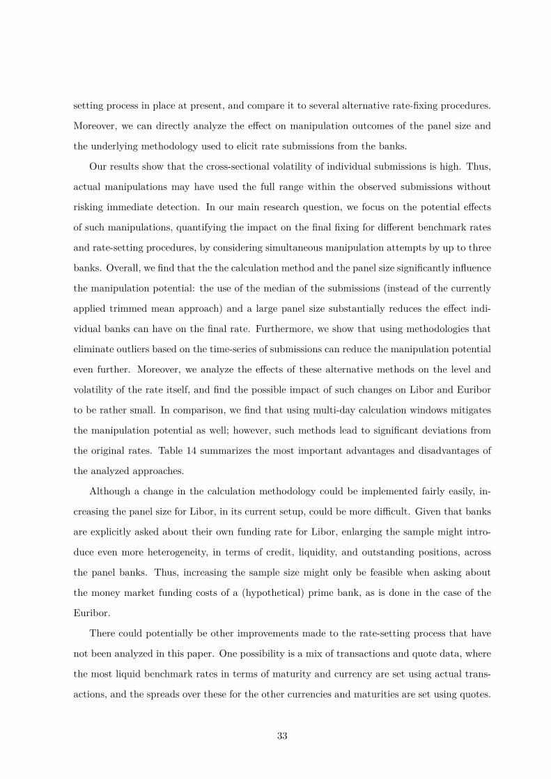
setting process in place at present, and compare it to several alternative rate-fixing procedures.

Moreover, we can directly analyze the effect on manipulation outcomes of the panel size and

the underlying methodology used to elicit rate submissions from the banks.

Our results show that the cross-sectional volatility of individual submissions is high. Thus,

actual manipulations may have used the full range within the observed submissions without

risking immediate detection. In our main research question, we focus on the potential effects

of such manipulations, quantifying the impact on the final fixing for different benchmark rates

and rate-setting procedures, by considering simultaneous manipulation attempts by up to three

banks. Overall, we find that the the calculation method and the panel size significantly influence

the manipulation potential: the use of the median of the submissions (instead of the currently

applied trimmed mean approach) and a large panel size substantially reduces the effect indi-

vidual banks can have on the final rate. Furthermore, we show that using methodologies that

eliminate outliers based on the time-series of submissions can reduce the manipulation potential

even further. Moreover, we analyze the effects of these alternative methods on the level and

volatility of the rate itself, and find the possible impact of such changes on Libor and Euribor

to be rather small. In comparison, we find that using multi-day calculation windows mitigates

the manipulation potential as well; however, such methods lead to significant deviations from

the original rates. Table 14 summarizes the most important advantages and disadvantages of

the analyzed approaches.

Although a change in the calculation methodology could be implemented fairly easily, in-

creasing the panel size for Libor, in its current setup, could be more difficult. Given that banks

are explicitly asked about their own funding rate for Libor, enlarging the sample might intro-

duce even more heterogeneity, in terms of credit, liquidity, and outstanding positions, across

the panel banks. Thus, increasing the sample size might only be feasible when asking about

the money market funding costs of a (hypothetical) prime bank, as is done in the case of the

Euribor.

There could potentially be other improvements made to the rate-setting process that have

not been analyzed in this paper. One possibility is a mix of transactions and quote data, where

the most liquid benchmark rates in terms of maturity and currency are set using actual trans-

actions, and the spreads over these for the other currencies and maturities are set using quotes.

33

Such alternatives can be analyzed once a complete transaction data set is available. However,

we find a clear need for an extensive transparency initiative that would make transaction report-

ing to a central database mandatory, as this would at least lead to the first step in validating

individual rate submissions and, thus, might allow a data-driven identification of manipulation

attempts.

34

A Robustness Checks (Internet Appendix)

A.1 Simulation Study of Manipulation Impact

In this appendix, we carry out a set of robustness checks using a simulation study. This setup

enables us to present our results in a controlled environment without needing to allow for

any strategic submissions by the panel banks. For that purpose, we model the distribution of

individual contributions. This allows us to simulate the banks’ submissions and analyze the

properties of different rate-setting methodologies. In particular, we estimate the manipulation

effects based on these simulated submissions and compare the results with the empirical data.

Even more importantly, the simulation provides us with the opportunity to investigate how the

manipulation impact changes if we apply our analyses to data that have already been manip-

ulated (see Section A.2). This addresses an issue related to the use of the actual submissions,

which may already be the result of manipulation.

We design the simulation study such that it resembles a representative case, by choosing to

mimic the 3M USD Libor. Thus, in our simulation, 16 banks contribute to the final rate by

submitting their individual submissions si (i.e., n = 16; this corresponds to the panel size of

the 3M USD Libor during most of the sample period). In a first step, we analyze the empirical

distribution of the banks’ contributions to 3M USD Libor in our data set, so as to derive a

suitable distribution function for the simulation study. For that purpose, we standardize the

individual submissions observed on each day, t, as they show a strong time-dependence:

si,t =si,t − µ̂t

σ̂t(3)

where µ̂t and σ̂t are the mean and standard deviation of the submissions on a given day,

respectively. Figure 8 shows the distribution of these standardized submissions. Overall, we

discover a symmetric distribution with fat tails. While this distribution does not strictly follow

any given theoretical distribution, it can be reasonably approximated using a Student’s t-

distribution, with the degrees of freedom chosen such that the kurtosis is approximately equal

to that of our estimated distribution.50 The estimated kurtosis is 1.56, which corresponds to50We tested different specifications, in particular the normal and log-normal distributions, but the results were

basically identical.

35

approximately df = 8 degrees of freedom. Thus, for each simulated day we draw n = 16

submissions according to:

si ∼ t(µ, σ, df) (4)

The set of n submissions will be denoted by s. We are interested in the manipulation

potential for the different rate-setting procedures analyzed in the prior sections. Therefore, we

define manipulation as in the previous sections: Let m be the number of manipulating banks,

then we set the m lowest submissions equal to the highest one. We denote the set of manipulated

contributions as sm:

sm := {s(i)}m<i≤n ∪mi=1 max(si, ..., sn) (5)

The function used to calculate the final fixing for each rate-setting methodology r is called

f r. The manipulation potential is thus calculated as

dr = f r(sm)− f r(s) (6)

In particular, this setup allows us to compare the manipulation effects for different rate-

setting procedures r. We calibrate the selected t-distribution such that it resembles an “average”

day in our sample period. To this end, we take the mean of the historic average of the 3M USD

Libor fixings during our sample period, given by µ = 235 bp. We set the standard deviation

equal to the average standard deviation of the daily submissions, i.e., σ = 3.42 bp. We estimate

the manipulation impact for the untrimmed mean, trimmed mean and median (we do not

present the random draw approach, as it basically provides the same impact as the trimmed

mean), and we show the results obtained using three manipulating banks. We produce 20, 000

scenarios (i.e., the number of simulated days) in our simulation. Table 15 shows the parameters

used for the simulation and the resulting manipulation potential.

The trimmed mean approach yields a simulated manipulation impact of 1.69 bp on average.

This value corresponds well with the one observed empirically (i.e., 1.61 bp). The simulation

confirms that the average manipulation impact is the highest when applying the untrimmed

mean, at 2.02 bp, and that when applying the median is the lowest, at 1.51 bp. In addition,

36

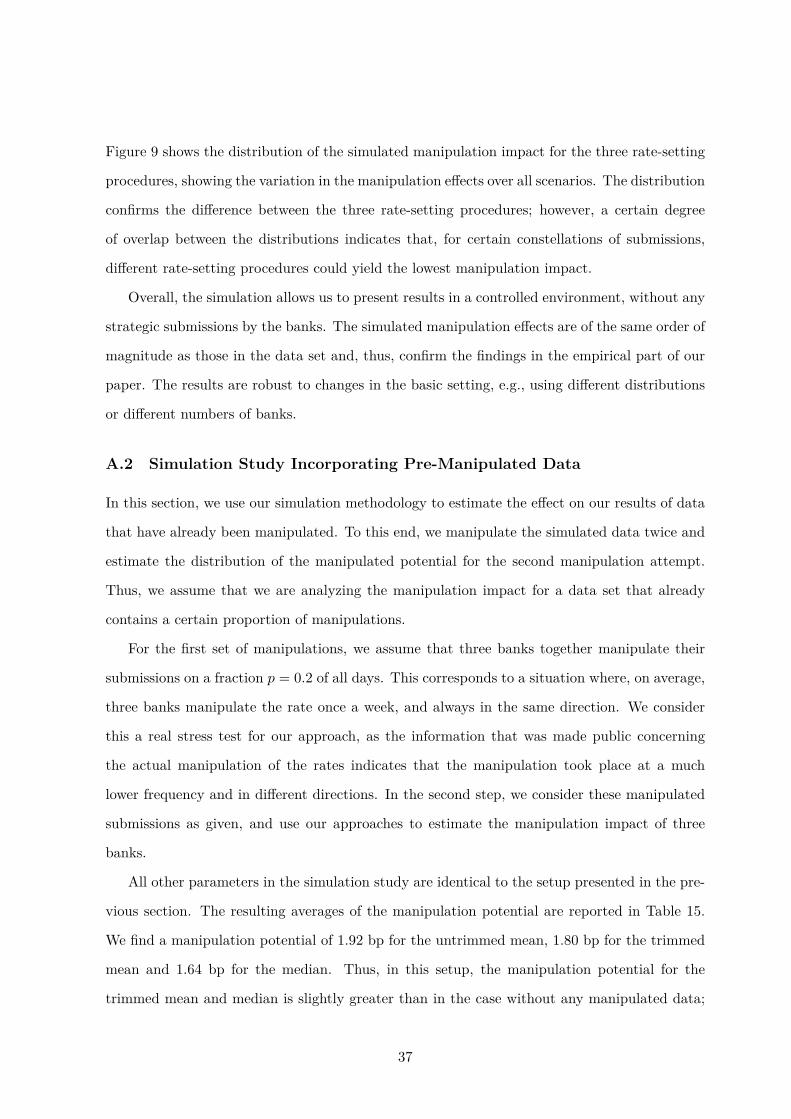
Figure 9 shows the distribution of the simulated manipulation impact for the three rate-setting

procedures, showing the variation in the manipulation effects over all scenarios. The distribution

confirms the difference between the three rate-setting procedures; however, a certain degree

of overlap between the distributions indicates that, for certain constellations of submissions,

different rate-setting procedures could yield the lowest manipulation impact.

Overall, the simulation allows us to present results in a controlled environment, without any

strategic submissions by the banks. The simulated manipulation effects are of the same order of

magnitude as those in the data set and, thus, confirm the findings in the empirical part of our

paper. The results are robust to changes in the basic setting, e.g., using different distributions

or different numbers of banks.

A.2 Simulation Study Incorporating Pre-Manipulated Data

In this section, we use our simulation methodology to estimate the effect on our results of data

that have already been manipulated. To this end, we manipulate the simulated data twice and

estimate the distribution of the manipulated potential for the second manipulation attempt.

Thus, we assume that we are analyzing the manipulation impact for a data set that already

contains a certain proportion of manipulations.

For the first set of manipulations, we assume that three banks together manipulate their

submissions on a fraction p = 0.2 of all days. This corresponds to a situation where, on average,

three banks manipulate the rate once a week, and always in the same direction. We consider

this a real stress test for our approach, as the information that was made public concerning

the actual manipulation of the rates indicates that the manipulation took place at a much

lower frequency and in different directions. In the second step, we consider these manipulated

submissions as given, and use our approaches to estimate the manipulation impact of three

banks.

All other parameters in the simulation study are identical to the setup presented in the pre-

vious section. The resulting averages of the manipulation potential are reported in Table 15.

We find a manipulation potential of 1.92 bp for the untrimmed mean, 1.80 bp for the trimmed

mean and 1.64 bp for the median. Thus, in this setup, the manipulation potential for the

trimmed mean and median is slightly greater than in the case without any manipulated data;

37

however, we find the manipulation impact to be of the same order of magnitude as before. Fur-

thermore, we still observe the same ranking when comparing different rate-setting procedures,

with the application of the median approach resulting in the lowest impact.

Figure 10 shows the density estimates for the manipulation potential using the pre-manipu-

lated submissions, providing further evidence that using underlying data containing a certain

proportion of manipulated contributions does not change the overall nature of the resulting

manipulation impact.

38

References

Abrantes-Metz, R. M. and Evans, D. S. (2012). Replacing the Libor with a transparent and

reliable index of interbank borrowing: Comments on the Wheatley Review of Libor initial

discussion paper. University of Chicago Institute for Law & Economics Olin Research Paper

No. 620.

Abrantes-Metz, R. M., Kraten, M., Metz, A. D., and Seos, G. S. (2012). Libor manipulation?

Journal of Banking & Finance, 36:136–150.

Abrantes-Metz, R. M., Villas-Boas, S. B., and Judge, G. (2011). Tracking the Libor rate.

Applied Economics Letters, 18:10:893–899.

Bessembinder, H., Maxwell, W., and Venkataraman, K. (2006). Market transparency, liquid-

ity externalities, and institutional trading costs in coporate bonds. Journal of Financial

Economics, 82:251–288.

British Bankers’ Association (2012). BBA Libor explained: The basics. http://www.bbalibor.

com/bbalibor-explained/the-basics.

Chen, J. (2013). Libor’s poker: Interbank borrowing costs and strategic reporting. Working

paper.

Coulter, B. and Shapiro, J. (2013). A mechanism for Libor. Working paper.

Duffie, D. and Dworczak, P. (2014). Robust benchmark design. Working paper.

Duffie, D., Skeie, D. R., and Vickery, J. I. (2013). A sampling-window approach to transactions-

based Libor fixing. Federal Reserve Bank of New York Staff Report Number 513.

Duffie, D. and Stein, J. C. (2015). Reforming Libor and other financial market benchmarks.

Journal of Economics Perspectives, 29(2):191–212.

Eaglesham, J. (2013). Bank made huge bet, and profit, on Libor. Wall Street Journal, Jan, 9.

Edwards, A., Harris, L., and Piwowar, M. (2007). Corporate bond market transaction costs

and transparency. Journal of Finance, 62:1421–1451.

39

European Banking Federation (2012). Euribor frequently asked questions. http://www.

euribor-ebf.eu/assets/files/Euribor%20FAQs%20Final.pdf.

Fouquau, J. and Spieser, P. K. (2015). Statistical evidence about Libor manipulation: A

”sherlock holmes” investigation. Journal of Banking & Finance, 50:632–643.

Friewald, N., Jankowitsch, R., and Subrahmanyam, M. (2012). Illiquidity or credit deterioration:

A study of liquidity in the US corporate bond market during financial crises. Journal of

Financial Economics, 105:18–36.

Friewald, N., Jankowitsch, R., and Subrahmanyam, M. (Forthcoming). Transparency and liq-

uidity in the structured product market. Review of Asset Pricing Studies.

Frunza, M. (2013). Market manipulation and moral hazard: Can the Libor be fixed? Working

paper.

Gandhi, P., Golez, B., Jackwerth, J. C., and Plazzi, A. (2016). Financial market misconduct

and public enforcement: The case of Libor manipulation. Working paper.

Goldstein, M., Hotchkiss, E., and Sirri, E. (2007). Transparency and liquidity: A controlled

experiment on corporate bonds. Review of Financial Studies, 20:235–273.

Green, R., Hollified, B., and Schürhoff, N. (2007). Dealer intermediation and price behavior in

the aftermarket for new bond issues. Journal of Financial Economics, 82:643–682.

Green, R. C. (2007). Presidential address: Issuers, underwriter syndicates, and aftermarket

transparency. Journal of Finance, 62:1529–1550.

Harris, L. and Piwowar, M. (2006). Secondary trading costs in the municipal bond market.

Journal of Finance, 61:1361–1397.

King, T. B. and Lewis, K. F. (2014). What drives bank funding spreads? Federal Reserve Bank

of Chicago WP 2014-23.

Kuo, D., Skeie, D. R., Vickery, J. I., and Youle, T. (2013). Identifing term interbank loans from

Fedwire payments data. FRB of New York Staff Report No. 603.

40

Kyle, A. S. and Viswanathan, S. (2008). How to define illegal price manipulation. American

Economic Review, 98:274–279.

Market Participants Group on Reforming Interest Rate Benchmarks (2014). Final report. http:

//www.financialstabilityboard.org/publications/r_140722b.pdf.

Mollencamp, C. and Whitehouse, M. (2008). Study casts doubt on key rate. Wall Street Journal,

May 29.

Snider, C. A. and Youle, T. (2014). The fix is in: Detecting portfolio driven manipulation of

the Libor. Working paper.

Wheatley, M. (2012a). The Wheatley Review of Libor: Final report. http://cdn.

hm-treasury.gov.uk/wheatley_review_libor_finalreport_280912.pdf.

Wheatley, M. (2012b). The Wheatley Review of Libor: Initial discussion paper. http://www.

hm-treasury.gov.uk/d/condoc_wheatley_review.pdf.

Youle, T. (2014). How much did manipulation distort the Libor? Working paper.

41

Figures

Jän 042005

Jul 032006

Jän 022008

Jul 012009

Jän 042011

Jul 022012

45

67

8

1) 3M AUD Libor

Per

cent

Jän 042005

Jul 032006

Jän 022008

Jul 012009

Jän 042011

Jul 022012

7.0

7.2

7.4

7.6

7.8

8.0

2) Panel Size

Num

ber

of P

anel

Ban

ks

Jän 042005

Jul 032006

Jän 022008

Jul 012009

Jän 042011

Jul 022012

010

2030

40

3) Std Deviation

Bas

is P

oint

s

Jän 042005

Jul 032006

Jän 022008

Jul 012009

Jän 042011

Jul 022012

020

4060

8010

012

0

4) Range

Bas

is P

oint

s

Figure 1. Descriptive statistics for the 3M AUD LiborThis figure shows the summary plots for the three month AUD Libor. Subfigure 1 shows the time-seriesof this reference rate. Subfigure 2 presents the panel size of banks contributing to the AUD Libor. Basedon the individual contributions, subfigures 3 and 4 show the cross-sectional standard deviation and therange, i.e., the difference between the highest and the lowest contribution, on each day. Our data setcontains the reference rate and the underlying contributions, obtained from Bloomberg for the timeperiod from January 2005 to December 2012.

42

Jan 042005

Jul 032006

Jan 022008

Jul 012009

Jan 042011

Jul 022012

12

34

51) 3M USD Libor

Per

cent

Jan 042005

Jul 032006

Jan 022008

Jul 012009

Jan 042011

Jul 022012

1617

1819

20

2) Panel Size

Num

ber

of P

anel

Ban

ks

Jan 042005

Jul 032006

Jan 022008

Jul 012009

Jan 042011

Jul 022012

010

2030

40

3) Std Deviation

Bas

is P

oint

s

Jan 042005

Jul 032006

Jan 022008

Jul 012009

Jan 042011

Jul 022012

050

100

150

4) Range

Bas

is P

oint

s

Figure 2. Descriptive statistics for the 3M USD LiborThis figure shows the summary plots for the three month USD Libor. Subfigure 1 shows the time-seriesof this reference rate. Subfigure 2 presents the panel size of banks contributing to the USD Libor. Basedon the individual contributions, subfigures 3 and 4 show the cross-sectional standard deviation and therange, i.e., the difference between the highest and the lowest contribution, on each day. Our data setcontains the reference rate and the underlying contributions, obtained from Bloomberg for the timeperiod from January 2005 to December 2012.

43

Jan 042005

Jul 032006

Jan 022008

Aug 032009

Feb 012011

Jul 312012

01

23

45

1) 3M Euribor

Per

cent

Jan 042005

Jul 032006

Jan 022008

Aug 032009

Feb 012011

Jul 312012

3840

4244

4648

2) Panel Size

Num

ber

of P

anel

Ban

ks

Jan 042005

Jul 032006

Jan 022008

Aug 032009

Feb 012011

Jul 312012

05

1015

3) Std Deviation

Bas

is P

oint

s

Jan 042005

Jul 032006

Jan 022008

Aug 032009

Feb 012011

Jul 312012

020

4060

8010

012

0

4) Range

Bas

is P

oint

s

Figure 3. Descriptive statistics for the 3M EuriborThis figure shows the summary plots for the three month Euribor. Subfigure 1 shows the time-series ofthis reference rate. Subfigure 2 presents the panel size of banks contributing to the Euribor. Based on theindividual contributions, subfigures 3 and 4 show the cross-sectional standard deviation and the range,i.e., the difference between the highest and the lowest contribution, on each day. Our data set containsthe reference rate and the underlying contributions, obtained from the European Banking Federation forthe time period from January 2005 to December 2012.

44

Jan 042005

Jul 032006

Jan 022008

Jul 012009

Jan 042011

Jul 022012

0.2

0.4

0.6

0.8

1.0

3M AUD Libor: Deutsche Bank

Rel

ativ

e R

ank

Jan 042005

Jul 032006

Jan 022008

Jul 012009

Jan 042011

Jul 022012

0.2

0.4

0.6

0.8

1.0

3M AUD Libor: Lloyds

Rel

ativ

e R

ank

Jan 042005

Jul 032006

Jan 022008

Jul 012009

Jan 042011

Jul 022012

0.2

0.4

0.6

0.8

1.0

3M USD Libor: JPM

Rel

ativ

e R

ank

Jan 042005

Jul 032006

Jan 022008

Jul 012009

Jan 042011

Jul 022012

0.2

0.4

0.6

0.8

1.0

3M USD Libor: Barclays

Rel

ativ

e R

ank

Jan 042005

Jul 032006

Jan 022008

Aug 032009

Aug 012011

0.0

0.2

0.4

0.6

0.8

1.0

3M Euribor: Citibank

Rel

ativ

e R

ank

Jan 042005

Jul 032006

Jan 022008

Aug 032009

Aug 012011

0.0

0.2

0.4

0.6

0.8

1.0

3M Euribor: Societe Generale

Rel

ativ

e R

ank

Figure 4. Ranks of panel banks’ contributionsThis figure shows the evolution of the ranks of selected panel banks’ contributions for the three monthAUD Libor, USD Libor and Euribor over time. To make the results comparable accross currencies,we standardize the ranks such that the bank with the highest rank (i.e., highest contribution) has arank of 1. For each reference rate, we present the results for two representative panel banks. Our dataset contains the reference rates and the underlying contributions, obtained from Bloomberg and theEuropean Banking Federation for the time period from January 2005 to December 2012.

45

Jan 042005

Jul 032006

Jan 022008

Jul 012009

Jan 042011

Jul 022012

−30

−20

−10

010

20

3M AUD Libor: Deutsche Bank

Spr

ead

in b

p

Jan 042005

Jul 032006

Jan 022008

Jul 012009

Jan 042011

Jul 022012

−10

0−

500

50

3M AUD Libor: Lloyds

Spr

ead

in b

p

Jan 042005

Jul 032006

Jan 022008

Jul 012009

Jan 042011

Jul 022012

−50

−40

−30

−20

−10

0

3M USD Libor: JPM

Spr

ead

in b

p

Jan 042005

Jul 032006

Jan 022008

Jul 012009

Jan 042011

Jul 022012

−20

020

4060

80

3M USD Libor: Barclays

Spr

ead

in b

p

Jan 042005

Jul 032006

Jan 022008

Aug 032009

Aug 012011

−30

−20

−10

010

3M Euribor: Citibank

Spr

ead

in b

p

Jan 042005

Jul 032006

Jan 022008

Aug 032009

Aug 012011

−40

−30

−20

−10

010

3M Euribor: Societe Generale

Spr

ead

in b

p

Figure 5. Difference between the final fixing and panel banks’ contributionsThis figure shows the difference between the individual contributions of selected panel banks and thefinal fixings for the three month AUD Libor, USD Libor and Euribor over time. For each reference rate,we present the results for two representative panel banks. Our data set contains the reference rates andthe underlying contributions, obtained from Bloomberg and the European Banking Federation for thetime period from January 2005 to December 2012.

46

Jan 042005

Jul 032006

Jan 022008

Jul 012009

Jan 042011

Jul 022012

05

1015

20

Impact of 1 Bank (AUD Libor)

Date

Impa

ct in

bp

Jan 042005

Jul 032006

Jan 022008

Jul 012009

Jan 042011

Jul 022012

05

1015

20

Impact of 2 Banks (AUD Libor)

Date

Impa

ct in

bp

Jan 042005

Jul 032006

Jan 022008

Jul 012009

Jan 042011

Jul 022012

05

1015

20

Impact of 3 Banks (AUD Libor)

Date

Impa

ct in

bp

Jan 042005

Jul 032006

Jan 022008

Jul 012009

Jan 042011

Jul 022012

05

1015

20

Impact of 1 Bank (USD Libor)

Date

Impa

ct in

bp

Jan 042005

Jul 032006

Jan 022008

Jul 012009

Jan 042011

Jul 022012

05

1015

20Impact of 2 Banks (USD Libor)

Date

Impa

ct in

bp

Jan 042005

Jul 032006

Jan 022008

Jul 012009

Jan 042011

Jul 022012

05

1015

20

Impact of 3 Banks (USD Libor)

Date

Impa

ct in

bp

Jan 042005

Jul 032006

Jan 022008

Aug 032009

Aug 012011

05

1015

20

Impact of 1 Bank (Euribor)

Impa

ct in

bp

Jan 042005

Jul 032006

Jan 022008

Aug 032009

Aug 012011

05

1015

20

Impact of 2 Banks (Euribor)

Impa

ct in

bp

Jan 042005

Jul 032006

Jan 022008

Aug 032009

Aug 012011

05

1015

20

Impact of 3 Banks (Euribor)

Impa

ct in

bp

Figure 6. Potential manipulation effectThis figure shows the potential manipulation impact using the current rate-setting methodology for thethree month AUD Libor, USD Libor and Euribor. For each day, we report the impact one, two or threecolluding banks could have on the final fixing. We use the following approach to quantify these effects:We start out with the observed individual contributions made by the panel banks to the final rate. Then,we change the lowest observed contribution, making it equal to the highest observed contribution, for thecase of a manipulation by one bank. The difference between the observed (historic) benchmark rate andthe resulting benchmark rate after changing this one contribution is our measure of the potential effect ofmanipulation. We use the same approach when considering the manipulation potential for two or threebanks, i.e., we set the lowest two (or three) contributions equal to the highest observed contribution.Our data set contains the reference rates and the underlying contributions, obtained from Bloombergand the European Banking Federation for the time period from January 2005 to December 2012.

47

..

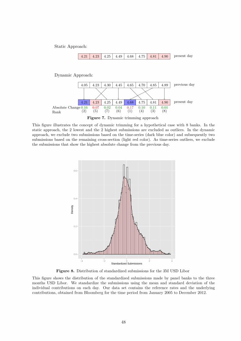
4.21

.

4.23

.

4.25

.

4.49

.

4.68

.

4.75

.

4.81

.

4.90

.

4.21

.

4.23

.

4.25

.

4.49

.

4.68

.

4.75

.

4.81

.

4.90

.

4.05

.

4.23

.

4.30

.

4.45

.

4.65

.

4.70

.

4.85

.

4.89

.

0.16

.

0.07

.

0.02

.

0.04

.

0.17

.

0.10

.

0.11

.

0.01

.

(2)

.

(5)

.

(7)

.

(6)

.

(1)

.

(4)

.

(3)

.

(8)

.

Absolute Change

.

Rank

.

present day

.

present day

.

previous day

.

Static Approach:

.Dynamic Approach:

Figure 7. Dynamic trimming approachThis figure illustrates the concept of dynamic trimming for a hypothetical case with 8 banks. In thestatic approach, the 2 lowest and the 2 highest submissions are excluded as outliers. In the dynamicapproach, we exclude two submissions based on the time-series (dark blue color) and subsequently twosubmissions based on the remaining cross-section (light red color). As time-series outliers, we excludethe submissions that show the highest absolute change from the previous day.

0.0

0.2

0.4

0.6

−4 −2 0 2 4Standardized Submissions

Den

sity

Figure 8. Distribution of standardized submissions for the 3M USD LiborThis figure shows the distribution of the standardized submissions made by panel banks to the threemonths USD Libor. We standardize the submissions using the mean and standard deviation of theindividual contributions on each day. Our data set contains the reference rates and the underlyingcontributions, obtained from Bloomberg for the time period from January 2005 to December 2012.

48

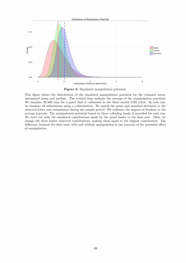
0.00

0.25

0.50

0.75

0 2 4 6 8Manipulation Potential in Basis Points

Den

sity Median

Trimmed

Untrimmed

Distribution of Manipulation Potential

Figure 9. Simulated manipulation potentialThis figure shows the distribution of the simulated manipulation potential for the trimmed mean,untrimmed mean and median. The vertical lines indicate the average of the manipulation potential.We simulate 20, 000 runs for a panel that is calibrated to the three month USD Libor. In each run,we simulate 16 submissions using a t-distribution. We match the mean and standard deviation to theobserved Libor rate submissions during the sample period. We calibrate the degrees of freedom to theaverage kurtosis. The manipulation potential based on three colluding banks is provided for each run:We start out with the simulated contributions made by the panel banks to the final rate. Then, wechange the three lowest observed contributions, making them equal to the highest contribution. Thedifference between the final rates with and without manipulation is our measure of the potential effectof manipulation.

49

0.0

0.2

0.4

0.6

0.8

0 2 4 6 8Manipulation Potential in Basis Points

Den

sity Median

Trimmed

Untrimmed

Distribution of Potential Manipulation In Presence of Pre−Manipulated Data

Figure 10. Simulated manipulation potential based on pre-manipulated dataThis figure shows the distribution of manipulation potential where we simulate pre-manipulated data,representing a robustness check as the observed empirical data may contain a certain degree of manip-ulation as well. The vertical lines show the average of the manipulation potential. We simulate 20, 000runs for a panel that is calibrated to the three month USD Libor. In each run, we simulate 16 sub-missions using a t-distribution. We match the mean and standard deviation to the observed Libor ratesubmissions during the sample period. We calibrate the degrees of freedom to the average kurtosis. Weassume that on a fraction of 0.2 of all days three banks manipulate the rate up. We then consider thesemanipulated submissions as given and we change the three lowest observed contributions, making themequal to the highest contribution. The difference between the final rates with and without this secondmanipulation is our measure of the manipulation potential in each run.

50

Tables

Table 1. Trimming approach for the Libor panelThis table shows the number of excluded bank submissions on each side of the Libor panel given theselected panel size. In principle, the highest and lowest 25% of all submissions are excluded. However, aparticular rounding approach is applied for non-integer numbers. For example for a panel of size 7, thehighest and lowest contributions are excluded, although 25% of the panel represents 1.75 contributions.This approach ensures that not more than 55% of the submissions are removed.

Panel size Nr. of excluded banks6 - 7 18 - 10 211 - 14 315 - 18 419 - 20 5

Table 2. Trimming approach for the Euribor panelThis table shows the number of excluded bank submissions on each side of the Euribor panel giventhe selected panel size. In principle, the highest and lowest 15% of all submissions are excluded. Thecommon method of rounding is applied to non-integer numbers. For example, for a panel of size 18, thethree highest and three lowest contributions are excluded.

Panel size Nr. of excluded banks12 - 16 217 - 23 324 - 29 430 - 36 537 - 43 644 - 45 7

Table 3. Effect on 3M AUD Libor rate when changing lowest submissionThis table shows the calculation of the three month AUD Libor rate on December 31, 2012. On this daythe AUD Libor panel consisted of 7 banks. Thus, the highest and lowest contributions were removed inthe trimming process. The first row shows the actual contributions on that day. The contributions ofbanks 2–6 are used to calculate the Libor rate, yielding a final fixing of 3.238%. In the second row, weillustrate the effect on this rate if a single contribution were different (e.g., because of manipulation). Ifthe bank with the lowest contribution (Bank 1) had instead submitted a contribution equal to that ofthe bank with the highest contribution (Bank 7), the fixing on that day would then be the average ofthe contributions of banks 3–7, i.e., the calculation window would shift by one bank. In this case, thefinal fixing would be 3.252%, an increase of 1.4 bp.

3.20 3.23 3.23 3.24 3.24 3.25 3.30

3.23 3.23 3.24 3.24 3.25 3.30 3.30

Bank 1

Bank 2

Bank 3

Bank 7

Bank 4

Bank 5

Bank 6

Bank 1

51

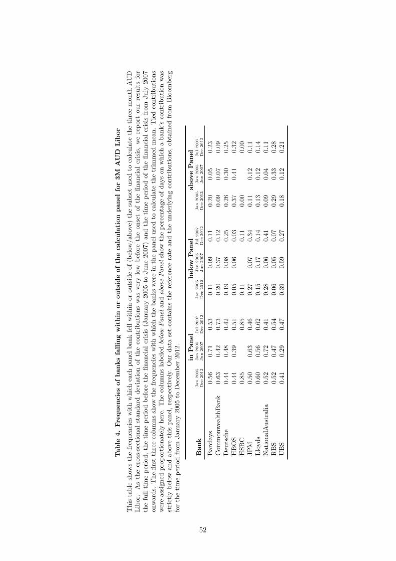
Tabl

e4.

Freq

uenc

ies

ofba

nks

falli

ngw

ithi

nor

outs

ide

ofth

eca

lcul

atio

npa

nelf

or3M

AU

DLi

bor

Thi

sta

ble

show

sth

efre

quen

cies

with

whi

chea

chpa

nelb

ank

fell

with

inor

outs

ide

of(b

elow

/abo

ve)

the

subs

etus

edto

calc

ulat

eth

eth

ree

mon

thA

UD

Libo

r.A

sth

ecr

oss-

sect

iona

lst

anda

rdde

viat

ion

ofth

eco

ntrib

utio

nswa

sve

rylo

wbe

fore

the

onse

tof

the

finan

cial

crisi

s,we

repo

rtou

rre

sults

for

the

full

time

perio

d,th

etim

epe

riod

befo

reth

efin

anci

alcr

isis

(Jan

uary

2005

toJu

ne20

07)

and

the

time

perio

dof

the

finan

cial

crisi

sfro

mJu

ly20

07on

ward

s.T

hefir

stth

ree

colu

mns

show

the

frequ

enci

esw

ithw

hich

the

bank

swe

rein

the

pane

luse

dto

calc

ulat

eth

etr

imm

edm

ean.

Tie

dco

ntrib

utio

nswe

reas

signe

dpr

opor

tiona

tely

here

.T

heco

lum

nsla

bele

dbe

low

Pane

land

abov

ePa

nels

how

the

perc

enta

geof

days

onw

hich

aba

nk’s

cont

ribut

ion

was

stric

tlybe

low

and

abov

eth

ispa

nel,

resp

ectiv

ely.

Our

data

set

cont

ains

the

refe

renc

era

tean

dth

eun

derly

ing

cont

ribut

ions

,obt

aine

dfro

mBl

oom

berg

for

the

time

perio

dfro

mJa

nuar

y20

05to

Dec

embe

r20

12.

inP

anel

belo

wP

anel

abov

eP

anel

Ban

kJa

n20

05Dec

2012

Jan20

05Ju

n20

07Ju

l20

07Dec

2012

Jan20

05Dec

2012

Jan20

05Ju

n20

07Ju

l20

07Dec

2012

Jan20

05Dec

2012

Jan20

05Ju

n20

07Ju

l20

07Dec

2012

Barc

lays

0.56

0.71

0.53

0.11

0.09

0.11

0.20

0.05

0.23

Com

mon

weal

thBa

nk0.

630.

420.

730.

200.

370.

120.

090.

070.

09D

euts

che

0.44

0.48

0.42

0.19

0.08

0.25

0.26

0.30

0.25

HBO

S0.

440.

390.

510.

050.

060.

030.

370.

410.

32H

SBC

0.85

0.85

0.11

0.11

0.00

0.00

JPM

0.50

0.63

0.46

0.27

0.07

0.34

0.11

0.12

0.11

Lloy

ds0.

600.

560.

620.

150.

170.

140.

130.

120.

14N

atio

nalA

ustr

alia

0.52

0.72

0.41

0.28

0.06

0.41

0.09

0.04

0.11

RBS

0.52

0.47

0.54

0.06

0.05

0.07

0.29

0.33

0.28

UBS

0.41

0.29

0.47

0.39

0.59

0.27

0.18

0.12

0.21

52

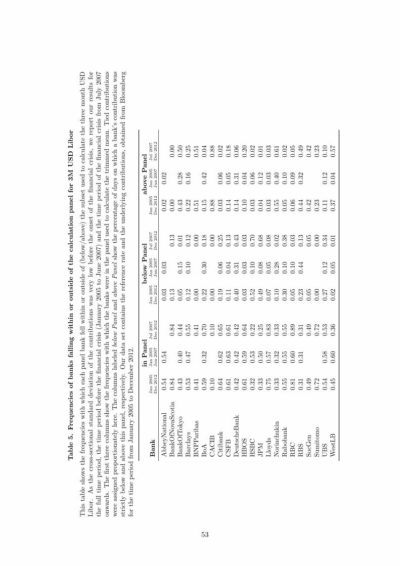
Tabl

e5.

Freq

uenc

ies

ofba

nks

falli

ngw

ithi

nor

outs

ide

ofth

eca

lcul

atio

npa

nelf

or3M

USD

Libo

rT

his

tabl

esh

ows

the

frequ

enci

esw

ithw

hich

each

pane

lban

kfe

llw

ithin

orou

tsid

eof

(bel

ow/a

bove

)th

esu

bset

used

toca

lcul

ate

the

thre

em

onth

USD

Libo

r.A

sth

ecr

oss-

sect

iona

lst

anda

rdde

viat

ion

ofth

eco

ntrib

utio

nswa

sve

rylo

wbe

fore

the

onse

tof

the

finan

cial

crisi

s,we

repo

rtou

rre

sults

for

the

full

time

perio

d,th

etim

epe

riod

befo

reth

efin

anci

alcr

isis

(Jan

uary

2005

toJu

ne20

07)

and

the

time

perio

dof

the

finan

cial

crisi

sfro

mJu

ly20

07on

ward

s.T

hefir

stth

ree

colu

mns

show

the

frequ

enci

esw

ithw

hich

the

bank

swe

rein

the

pane

luse

dto

calc

ulat

eth

etr

imm

edm

ean.

Tie

dco

ntrib

utio

nswe

reas

signe

dpr

opor

tiona

tely

here

.T

heco

lum

nsla

bele

dbe

low

Pane

land

abov

ePa

nels

how

the

perc

enta

geof

days

onw

hich

aba

nk’s

cont

ribut

ion

was

stric

tlybe

low

and

abov

eth

ispa

nel,

resp

ectiv

ely.

Our

data

set

cont

ains

the

refe

renc

era

tean

dth

eun

derly

ing

cont

ribut

ions

,obt

aine

dfro

mBl

oom

berg

for

the

time

perio

dfro

mJa

nuar

y20

05to

Dec

embe

r20

12.

inP

anel

belo

wP

anel

abov

eP

anel

Ban

kJa

n20

05Dec

2012

Jan20

05Ju

n20

07Ju

l20

07Dec

2012

Jan20

05Dec

2012

Jan20

05Ju

n20

07Ju

l20

07Dec

2012

Jan20

05Dec

2012

Jan20

05Ju

n20

07Ju

l20

07Dec

2012

Abb

eyN

atio

nal

0.54

0.54

0.03

0.03

0.02

0.02

Bank

OfN

ovaS

cotia

0.84

0.84

0.13

0.13

0.00

0.00

Bank

OfT

okyo

0.43

0.40

0.44

0.05

0.15

0.01

0.43

0.28

0.50

Barc

lays

0.53

0.47

0.55

0.12

0.10

0.12

0.22

0.16

0.25

BNPP

arib

as0.

410.

410.

000.

000.

510.

51Bo

A0.

590.

320.

700.

220.

300.

180.

150.

420.

04C

AC

IB0.

100.

100.

000.

000.

880.

88C

itiba

nk0.

640.

620.

650.

190.

060.

250.

030.

060.

02C

SFB

0.61

0.63

0.61

0.11

0.04

0.13

0.14

0.05

0.18

Deu

tsch

eBan

k0.

420.

420.

420.

400.

310.

430.

140.

310.

06H

BOS

0.61

0.59

0.64

0.03

0.03

0.03

0.10

0.04

0.20

HSB

C0.

320.

530.

220.

520.

100.

700.

030.

060.

02JP

M0.

330.

500.

250.

490.

080.

680.

040.

120.

01Ll

oyds

0.75

0.57

0.83

0.07

0.05

0.08

0.03

0.03

0.03

Nor

inch

ukin

0.33

0.32

0.33

0.10

0.28

0.02

0.55

0.40

0.61

Rab

oban

k0.

550.

550.

550.

300.

100.

380.

050.

100.

02R

BC0.

810.

600.

890.

050.

100.

030.

060.

090.

05R

BS0.

310.

310.

310.

230.

440.

130.

440.

320.

49So

cGen

0.49

0.49

0.05

0.05

0.42

0.42

Sum

itom

o0.

720.

720.

000.

000.

230.

23U

BS0.

540.

580.

530.

270.

120.

340.

110.

120.

10W

estL

B0.

450.

600.

360.

020.

050.

010.

370.

040.

57

53

Tabl

e6.

Freq

uenc

ies

ofba

nks

falli

ngw

ithi

nor

outs

ide

ofth

eca

lcul

atio

npa

nelf

or3M

Eur

ibor

Thi

stab

lesh

owst

hefre

quen

cies

with

whi

chea

chpa

nelb

ank

fell

with

inor

outs

ide

of(b

elow

/abo

ve)t

hesu

bset

used

toca

lcul

ate

the

thre

em

onth

Eurib

or.

As

the

cros

s-se

ctio

nals

tand

ard

devi

atio

nof

the

cont

ribut

ions

was

very

low

befo

reth

eon

set

ofth

efin

anci

alcr

isis,

were

port

our

resu

ltsfo

rth

efu

lltim

epe

riod,

the

time

perio

dbe

fore

the

finan

cial

crisi

s(J

anua

ry20

05to

June

2007

)an

dth

etim

epe

riod

ofth

efin

anci

alcr

isis

from

July

2007

onwa

rds.

The

first

thre

eco

lum

nssh

owth

efre

quen

cies

with

whi

chth

eba

nks

were

inth

epa

nelu

sed

toca

lcul

ate

the

trim

med

mea

n.T

ied

cont

ribut

ions

were

assig

ned

prop

ortio

nate

lyhe

re.

The

colu

mns

labe

led

belo

wPa

nela

ndab

ove

Pane

lsho

wth

epe

rcen

tage

ofda

yson

whi

cha

bank

’sco

ntrib

utio

nwa

sst

rictly

belo

wan

dab

ove

this

pane

l,re

spec

tivel

y.O

urda

tase

tco

ntai

nsth

ere

fere

nce

rate

and

the

unde

rlyin

gco

ntrib

utio

ns,

obta

ined

from

the

Euro

pean

Bank

ing

Fede

ratio

nfo

rth

etim

epe

riod

from

Janu

ary

2005

toD

ecem

ber

2012

.in

Pan

elb

elow

Pan

elab

ove

Pan

elB

ank

Jan20

05Dec

2012

Jan20

05Ju

n20

07Ju

l20

07Dec

2012

Jan20

05Dec

2012

Jan20

05Ju

n20

07Ju

l20

07Dec

2012

Jan20

05Dec

2012

Jan20

05Ju

n20

07Ju

l20

07Dec

2012

ABN

Amro

0.68

0.73

0.62

0.07

0.05

0.09

0.14

0.06

0.22

AIB

Group

0.50

0.79

0.37

0.01

0.03

0.00

0.39

0.02

0.55

Ban

caIntesa

0.87

0.80

0.90

0.02

0.01

0.02

0.01

0.01

0.01

Ban

caMPS

0.86

0.70

0.94

0.03

0.07

0.01

0.06

0.12

0.03

Ban

coBilb

ao0.47

0.13

0.62

0.24

0.53

0.12

0.38

0.73

0.22

Ban

coSa

ntan

der

0.77

0.79

0.76

0.06

0.05

0.07

0.08

0.03

0.10

Ban

kof

Irelan

d0.87

0.77

0.92

0.03

0.05

0.02

0.03

0.04

0.02

Ban

kof

Tok

yoMitsubishi

0.49

0.31

0.57

0.38

0.38

0.38

0.17

0.52

0.00

Ban

quePostale

0.62

0.62

0.19

0.19

0.15

0.15

Barclay

s0.71

0.78

0.68

0.16

0.06

0.20

0.06

0.05

0.07

BayernLB

0.63

0.43

0.73

0.24

0.39

0.17

0.12

0.28

0.05

BCEE

0.84

0.81

0.86

0.07

0.01

0.10

0.01

0.01

0.00

Belfiu

s0.63

0.77

0.55

0.02

0.01

0.02

0.25

0.02

0.38

BNL

0.76

0.76

0.06

0.06

0.05

0.05

BNP

Paribas

0.50

0.57

0.47

0.33

0.27

0.35

0.12

0.17

0.10

Cap

ita

0.87

0.87

0.90

0.00

0.00

0.00

0.00

0.00

0.02

Cecab

ank

0.59

0.74

0.52

0.08

0.06

0.08

0.23

0.07

0.31

Cecab

ank

0.00

0.00

0.00

0.00

0.00

0.00

CGD

0.64

0.80

0.57

0.01

0.01

0.01

0.26

0.01

0.38

CIC

0.59

0.59

0.58

0.20

0.18

0.21

0.14

0.19

0.12

Citiban

k0.56

0.50

0.58

0.33

0.33

0.33

0.07

0.21

0.01

Com

merzb

ank

0.87

0.67

0.96

0.06

0.15

0.01

0.03

0.09

0.01

Credite

AgricoleCIB

0.69

0.80

0.64

0.16

0.01

0.23

0.05

0.02

0.06

Dan

skeBan

k0.81

0.79

0.82

0.06

0.01

0.09

0.04

0.01

0.05

DekaBan

k0.07

0.07

0.00

0.00

0.84

0.84

Deu

tscheBan

k0.39

0.42

0.38

0.40

0.40

0.39

0.23

0.32

0.18

Dexia

0.71

0.71

0.09

0.09

0.17

0.17

Dresdne

rBan

k0.83

0.77

0.92

0.02

0.03

0.01

0.02

0.01

0.02

DZBan

k0.58

0.75

0.50

0.20

0.07

0.25

0.14

0.07

0.16

Erste

Ban

k0.43

0.73

0.29

0.02

0.07

0.00

0.45

0.09

0.62

Fortis

0.63

0.55

0.70

0.11

0.19

0.03

0.25

0.27

0.22

HSB

C0.67

0.68

0.67

0.20

0.11

0.24

0.08

0.16

0.05

HVB

0.78

0.78

0.06

0.06

0.05

0.05

ING

0.86

0.77

0.90

0.04

0.05

0.04

0.04

0.06

0.03

JPM

0.52

0.72

0.44

0.35

0.06

0.49

0.03

0.08

0.00

KBC

0.80

0.82

0.79

0.02

0.03

0.01

0.11

0.02

0.15

laCaixa

0.97

0.97

0.00

0.00

0.01

0.01

LB

Bad

en-W

ürttem

berg

0.79

0.71

0.82

0.08

0.10

0.08

0.05

0.06

0.05

LB

Berlin

0.90

0.81

0.95

0.02

0.04

0.01

0.02

0.02

0.01

LB

Hessen-Thü

ring

en0.78

0.80

0.76

0.01

0.03

0.00

0.12

0.03

0.16

Natexis

0.69

0.71

0.61

0.09

0.08

0.13

0.11

0.09

0.19

Nationa

lBan

kof

Greece

0.84

0.82

0.85

0.01

0.01

0.00

0.07

0.02

0.09

Natixis

0.69

0.62

0.72

0.09

0.18

0.05

0.17

0.17

0.17

Norde

a0.93

0.80

0.99

0.00

0.01

0.00

0.00

0.01

0.00

NordLB

0.73

0.72

0.74

0.12

0.11

0.12

0.08

0.09

0.07

Poh

jola

0.96

0.96

0.03

0.03

0.00

0.00

Rab

oban

k0.60

0.77

0.52

0.31

0.03

0.43

0.01

0.02

0.01

RBI

0.82

0.80

0.84

0.07

0.00

0.10

0.01

0.00

0.01

RBS

0.84

0.84

0.09

0.09

0.05

0.05

Sanp

aolo

IMI

0.90

0.90

0.00

0.00

0.00

0.00

SocieteGen

erale

0.58

0.43

0.64

0.18

0.29

0.13

0.22

0.40

0.13

Sven

ska

0.90

0.82

0.93

0.01

0.02

0.00

0.03

0.02

0.03

UBIBan

ca1.00

1.00

0.00

0.00

0.00

0.00

UBS

0.56

0.73

0.48

0.21

0.08

0.27

0.16

0.05

0.20

Unicred

it0.88

0.80

0.91

0.03

0.02

0.04

0.02

0.02

0.02

WestLB

0.77

0.70

0.81

0.04

0.10

0.01

0.12

0.09

0.13

54

Table 7. Rank changes of banks for 3M AUD LiborThis table shows the mean and standard deviation of the daily absolute rank changes for the panelbanks contributing to the three month AUD Libor. As the cross-sectional standard deviation of thecontributions was very low before the onset of the financial crisis, we report our results for the full timeperiod, the time period before the financial crisis (January 2005 to June 2007) and the time periodof the financial crisis from July 2007 onwards. To make the results comparable across currencies, westandardize the ranks such that the bank with the highest rank (i.e., highest contribution) has a rankof 1. For example, a rank change of 0.25 means that a bank’s rank change corresponds to a quarterof the panel. Our data set contains the reference rate and the underlying contributions, obtained fromBloomberg for the time period from January 2005 to December 2012.

Mean StdDevBank Jan 2005

Dec 2012Jan 2005Jun 2007

Jul 2007Dec 2012

Jan 2005Dec 2012

Jan 2005Jun 2007

Jul 2007Dec 2012

Barclays 0.13 0.20 0.12 0.16 0.16 0.16CommonwealthBank 0.17 0.15 0.18 0.17 0.15 0.18Deutsche 0.11 0.13 0.10 0.14 0.14 0.14HBOS 0.18 0.18 0.19 0.18 0.19 0.17HSBC 0.07 0.07 0.10 0.10JPM 0.11 0.20 0.08 0.16 0.18 0.13Lloyds 0.16 0.18 0.14 0.18 0.17 0.18NationalAustralia 0.15 0.18 0.13 0.16 0.15 0.17RBS 0.13 0.16 0.12 0.16 0.16 0.16UBS 0.12 0.10 0.13 0.16 0.13 0.17

55

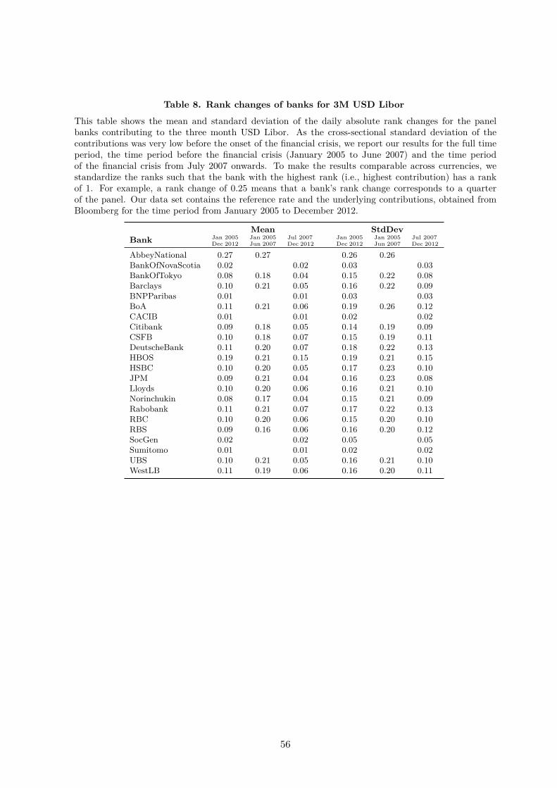
Table 8. Rank changes of banks for 3M USD LiborThis table shows the mean and standard deviation of the daily absolute rank changes for the panelbanks contributing to the three month USD Libor. As the cross-sectional standard deviation of thecontributions was very low before the onset of the financial crisis, we report our results for the full timeperiod, the time period before the financial crisis (January 2005 to June 2007) and the time periodof the financial crisis from July 2007 onwards. To make the results comparable across currencies, westandardize the ranks such that the bank with the highest rank (i.e., highest contribution) has a rankof 1. For example, a rank change of 0.25 means that a bank’s rank change corresponds to a quarterof the panel. Our data set contains the reference rate and the underlying contributions, obtained fromBloomberg for the time period from January 2005 to December 2012.

Mean StdDevBank Jan 2005

Dec 2012Jan 2005Jun 2007

Jul 2007Dec 2012

Jan 2005Dec 2012

Jan 2005Jun 2007

Jul 2007Dec 2012

AbbeyNational 0.27 0.27 0.26 0.26BankOfNovaScotia 0.02 0.02 0.03 0.03BankOfTokyo 0.08 0.18 0.04 0.15 0.22 0.08Barclays 0.10 0.21 0.05 0.16 0.22 0.09BNPParibas 0.01 0.01 0.03 0.03BoA 0.11 0.21 0.06 0.19 0.26 0.12CACIB 0.01 0.01 0.02 0.02Citibank 0.09 0.18 0.05 0.14 0.19 0.09CSFB 0.10 0.18 0.07 0.15 0.19 0.11DeutscheBank 0.11 0.20 0.07 0.18 0.22 0.13HBOS 0.19 0.21 0.15 0.19 0.21 0.15HSBC 0.10 0.20 0.05 0.17 0.23 0.10JPM 0.09 0.21 0.04 0.16 0.23 0.08Lloyds 0.10 0.20 0.06 0.16 0.21 0.10Norinchukin 0.08 0.17 0.04 0.15 0.21 0.09Rabobank 0.11 0.21 0.07 0.17 0.22 0.13RBC 0.10 0.20 0.06 0.15 0.20 0.10RBS 0.09 0.16 0.06 0.16 0.20 0.12SocGen 0.02 0.02 0.05 0.05Sumitomo 0.01 0.01 0.02 0.02UBS 0.10 0.21 0.05 0.16 0.21 0.10WestLB 0.11 0.19 0.06 0.16 0.20 0.11

56

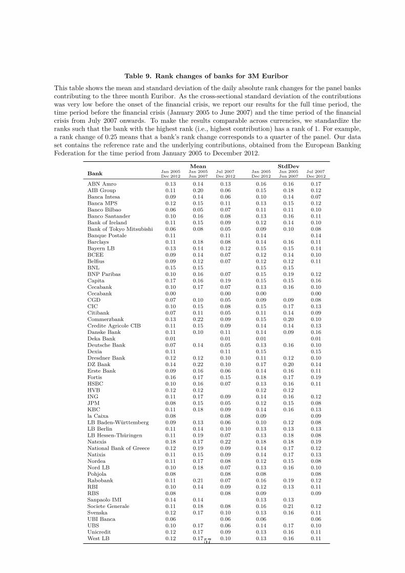
Table 9. Rank changes of banks for 3M EuriborThis table shows the mean and standard deviation of the daily absolute rank changes for the panel bankscontributing to the three month Euribor. As the cross-sectional standard deviation of the contributionswas very low before the onset of the financial crisis, we report our results for the full time period, thetime period before the financial crisis (January 2005 to June 2007) and the time period of the financialcrisis from July 2007 onwards. To make the results comparable across currencies, we standardize theranks such that the bank with the highest rank (i.e., highest contribution) has a rank of 1. For example,a rank change of 0.25 means that a bank’s rank change corresponds to a quarter of the panel. Our dataset contains the reference rate and the underlying contributions, obtained from the European BankingFederation for the time period from January 2005 to December 2012.

Mean StdDevBank Jan 2005

Dec 2012Jan 2005Jun 2007

Jul 2007Dec 2012

Jan 2005Dec 2012

Jan 2005Jun 2007

Jul 2007Dec 2012

ABN Amro 0.13 0.14 0.13 0.16 0.16 0.17AIB Group 0.11 0.20 0.06 0.15 0.18 0.12Banca Intesa 0.09 0.14 0.06 0.10 0.14 0.07Banca MPS 0.12 0.15 0.11 0.13 0.15 0.12Banco Bilbao 0.06 0.05 0.07 0.11 0.11 0.10Banco Santander 0.10 0.16 0.08 0.13 0.16 0.11Bank of Ireland 0.11 0.15 0.09 0.12 0.14 0.10Bank of Tokyo Mitsubishi 0.06 0.08 0.05 0.09 0.10 0.08Banque Postale 0.11 0.11 0.14 0.14Barclays 0.11 0.18 0.08 0.14 0.16 0.11Bayern LB 0.13 0.14 0.12 0.15 0.15 0.14BCEE 0.09 0.14 0.07 0.12 0.14 0.10Belfius 0.09 0.12 0.07 0.12 0.12 0.11BNL 0.15 0.15 0.15 0.15BNP Paribas 0.10 0.16 0.07 0.15 0.19 0.12Capita 0.17 0.16 0.19 0.15 0.15 0.16Cecabank 0.10 0.17 0.07 0.13 0.16 0.10Cecabank 0.00 0.00 0.00 0.00CGD 0.07 0.10 0.05 0.09 0.09 0.08CIC 0.10 0.15 0.08 0.15 0.17 0.13Citibank 0.07 0.11 0.05 0.11 0.14 0.09Commerzbank 0.13 0.22 0.09 0.15 0.20 0.10Credite Agricole CIB 0.11 0.15 0.09 0.14 0.14 0.13Danske Bank 0.11 0.10 0.11 0.14 0.09 0.16Deka Bank 0.01 0.01 0.01 0.01Deutsche Bank 0.07 0.14 0.05 0.13 0.16 0.10Dexia 0.11 0.11 0.15 0.15Dresdner Bank 0.12 0.12 0.10 0.11 0.12 0.10DZ Bank 0.14 0.22 0.10 0.17 0.20 0.14Erste Bank 0.09 0.16 0.06 0.14 0.16 0.11Fortis 0.16 0.17 0.15 0.18 0.17 0.19HSBC 0.10 0.16 0.07 0.13 0.16 0.11HVB 0.12 0.12 0.12 0.12ING 0.11 0.17 0.09 0.14 0.16 0.12JPM 0.08 0.15 0.05 0.12 0.15 0.08KBC 0.11 0.18 0.09 0.14 0.16 0.13la Caixa 0.08 0.08 0.09 0.09LB Baden-Württemberg 0.09 0.13 0.06 0.10 0.12 0.08LB Berlin 0.11 0.14 0.10 0.13 0.13 0.13LB Hessen-Thüringen 0.11 0.19 0.07 0.13 0.18 0.08Natexis 0.18 0.17 0.22 0.18 0.18 0.19National Bank of Greece 0.12 0.19 0.09 0.14 0.17 0.12Natixis 0.11 0.15 0.09 0.14 0.17 0.13Nordea 0.11 0.17 0.08 0.12 0.15 0.08Nord LB 0.10 0.18 0.07 0.13 0.16 0.10Pohjola 0.08 0.08 0.08 0.08Rabobank 0.11 0.21 0.07 0.16 0.19 0.12RBI 0.10 0.14 0.09 0.12 0.13 0.11RBS 0.08 0.08 0.09 0.09Sanpaolo IMI 0.14 0.14 0.13 0.13Societe Generale 0.11 0.18 0.08 0.16 0.21 0.12Svenska 0.12 0.17 0.10 0.13 0.16 0.11UBI Banca 0.06 0.06 0.06 0.06UBS 0.10 0.17 0.06 0.14 0.17 0.10Unicredit 0.12 0.17 0.09 0.13 0.16 0.11West LB 0.12 0.17 0.10 0.13 0.16 0.1157

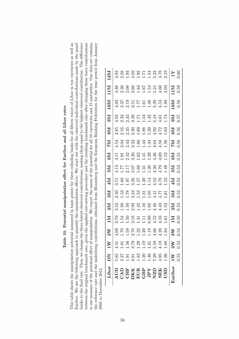
Tabl

e10

.P

oten

tial

man

ipul

atio

neff

ect

for

Eur

ibor

and

allL

ibor

rate

sT

his

tabl

esh

ows

the

man

ipul

atio

npo

tent

ialm

easu

red

inba

sispo

ints

for

thre

eco

lludi

ngba

nks

for

allfi

fteen

teno

rsof

Libo

rin

ten

curr

enci

esas

well

asEu

ribor

.W

eus

eth

efo

llow

ing

appr

oach

toqu

antif

yth

em

anip

ulat

ion

effec

ts:W

est

arto

utw

ithth

eob

serv

edin

divi

dual

cont

ribut

ions

mad

eby

the

pane

lba

nkst

oth

efin

alra

te.T

hen,

wech

ange

the

thre

elo

west

obse

rved

cont

ribut

ions

,mak

ing

them

equa

lto

the

high

esto

bser

ved

cont

ribut

ion.

The

diffe

renc

ebe

twee

nth

eor

igin

albe

nchm

ark

rate

,giv

enth

eap

plie

dra

te-s

ettin

gpr

oced

ure

and

the

resu

lting

benc

hmar

kra

teaf

terc

hang

ing

thes

eth

ree

cont

ribut

ions

isou

rmea

sure

ofth

epo

tent

iale

ffect

ofm

anip

ulat

ion.

We

repo

rtth

em

ean

ofth

epo

tent

ialf

oral

l10

curr

enci

esan

d15

mat

uriti

es.

Our

data

setc

onta

ins

the

refe

renc

era

tean

dth

eun

derly

ing

cont

ribut

ions

,obt

aine

dfro

mBl

oom

berg

and

the

Euro

pean

Bank

ing

Fede

ratio

nfo

rth

etim

epe

riod

from

Janu

ary

2005

toD

ecem

ber

2012

.

Libo

rO

N1W

2W1M

2M3M

4M5M

6M7M

8M9M

10M

11M

12M

AU

D5.

854.

414.

093.

793.

523.

503.

714.

134.

114.

544.

854.

824.

934.

864.

82C

AD

2.27

1.81

1.70

1.54

1.50

1.53

1.68

1.77

1.91

2.04

2.16

2.32

2.37

2.30

2.28

CH

F1.

911.

561.

591.

501.

501.

781.

972.

172.

422.

432.

352.

322.

192.

081.

93D

KK

8.01

3.79

3.70

3.18

2.93

3.24

3.26

3.07

3.20

3.23

3.30

3.39

3.51

3.66

4.02

EU

R1.

821.

291.

321.

311.

421.

531.

571.

601.

621.

661.

691.

711.

771.

841.

92G

BP

1.20

1.19

1.20

1.11

1.16

1.31

1.30

1.31

1.41

1.43

1.88

1.54

1.61

1.67

1.71

JPY

1.46

1.31

1.19

0.99

1.02

1.05

1.14

1.20

1.29

1.34

1.39

1.42

1.46

1.54

1.54

NZD

7.29

5.58

4.98

4.72

4.48

4.41

4.52

4.30

4.36

4.64

4.92

5.18

5.39

5.21

5.23

SEK

4.95

4.18

4.20

4.16

4.43

4.77

4.78

4.79

4.69

4.58

4.72

4.61

4.53

4.60

4.78

USD

1.90

1.88

1.84

1.61

1.53

1.61

1.52

1.49

1.52

1.56

1.63

1.74

1.89

2.03

2.19

Eur

ibor

1W2W

3W1M

2M3M

4M5M

6M7M

8M9M

10M

11M

1Y0.

550.

530.

540.

500.

530.

530.

530.

530.

550.

560.

560.

570.

580.

590.

60

58

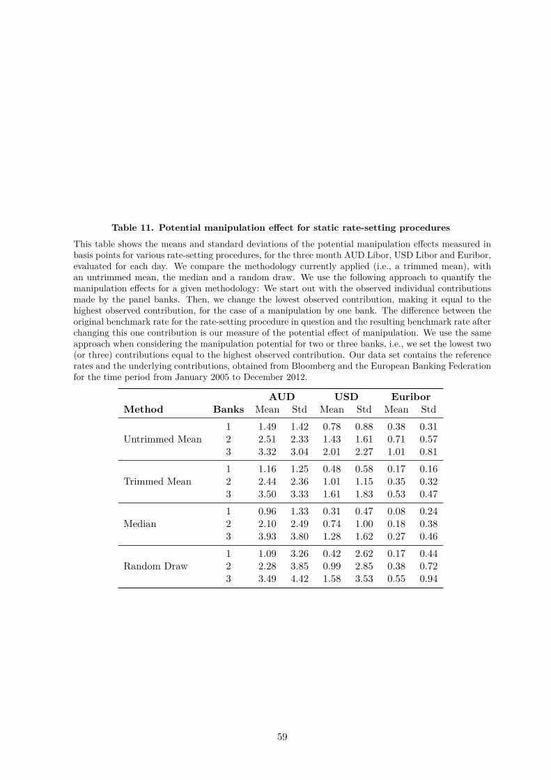
Table 11. Potential manipulation effect for static rate-setting proceduresThis table shows the means and standard deviations of the potential manipulation effects measured inbasis points for various rate-setting procedures, for the three month AUD Libor, USD Libor and Euribor,evaluated for each day. We compare the methodology currently applied (i.e., a trimmed mean), withan untrimmed mean, the median and a random draw. We use the following approach to quantify themanipulation effects for a given methodology: We start out with the observed individual contributionsmade by the panel banks. Then, we change the lowest observed contribution, making it equal to thehighest observed contribution, for the case of a manipulation by one bank. The difference between theoriginal benchmark rate for the rate-setting procedure in question and the resulting benchmark rate afterchanging this one contribution is our measure of the potential effect of manipulation. We use the sameapproach when considering the manipulation potential for two or three banks, i.e., we set the lowest two(or three) contributions equal to the highest observed contribution. Our data set contains the referencerates and the underlying contributions, obtained from Bloomberg and the European Banking Federationfor the time period from January 2005 to December 2012.

AUD USD EuriborMethod Banks Mean Std Mean Std Mean Std

Untrimmed Mean1 1.49 1.42 0.78 0.88 0.38 0.312 2.51 2.33 1.43 1.61 0.71 0.573 3.32 3.04 2.01 2.27 1.01 0.81

Trimmed Mean1 1.16 1.25 0.48 0.58 0.17 0.162 2.44 2.36 1.01 1.15 0.35 0.323 3.50 3.33 1.61 1.83 0.53 0.47

Median1 0.96 1.33 0.31 0.47 0.08 0.242 2.10 2.49 0.74 1.00 0.18 0.383 3.93 3.80 1.28 1.62 0.27 0.46

Random Draw1 1.09 3.26 0.42 2.62 0.17 0.442 2.28 3.85 0.99 2.85 0.38 0.723 3.49 4.42 1.58 3.53 0.55 0.94

59

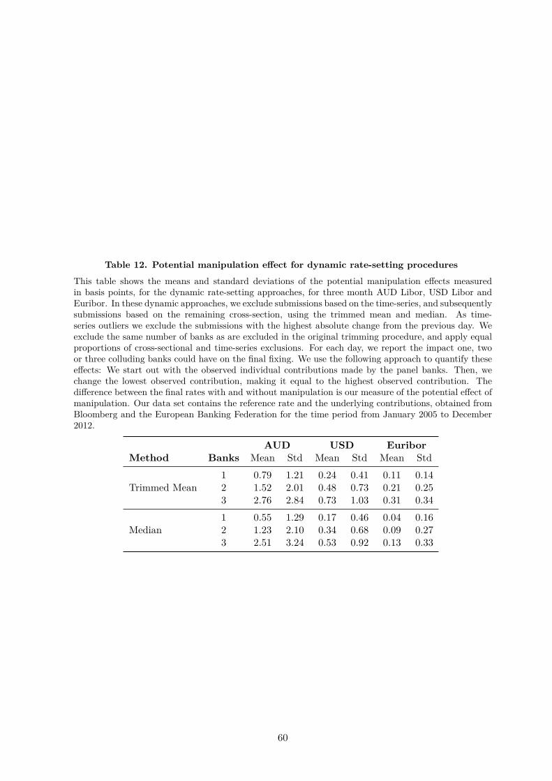
Table 12. Potential manipulation effect for dynamic rate-setting proceduresThis table shows the means and standard deviations of the potential manipulation effects measuredin basis points, for the dynamic rate-setting approaches, for three month AUD Libor, USD Libor andEuribor. In these dynamic approaches, we exclude submissions based on the time-series, and subsequentlysubmissions based on the remaining cross-section, using the trimmed mean and median. As time-series outliers we exclude the submissions with the highest absolute change from the previous day. Weexclude the same number of banks as are excluded in the original trimming procedure, and apply equalproportions of cross-sectional and time-series exclusions. For each day, we report the impact one, twoor three colluding banks could have on the final fixing. We use the following approach to quantify theseeffects: We start out with the observed individual contributions made by the panel banks. Then, wechange the lowest observed contribution, making it equal to the highest observed contribution. Thedifference between the final rates with and without manipulation is our measure of the potential effect ofmanipulation. Our data set contains the reference rate and the underlying contributions, obtained fromBloomberg and the European Banking Federation for the time period from January 2005 to December2012.

AUD USD EuriborMethod Banks Mean Std Mean Std Mean Std

Trimmed Mean1 0.79 1.21 0.24 0.41 0.11 0.142 1.52 2.01 0.48 0.73 0.21 0.253 2.76 2.84 0.73 1.03 0.31 0.34

Median1 0.55 1.29 0.17 0.46 0.04 0.162 1.23 2.10 0.34 0.68 0.09 0.273 2.51 3.24 0.53 0.92 0.13 0.33

60

Table 13. Potential manipulation effects for multi-day window proceduresThis table shows the means and standard deviations of the potential manipulation effects measured inbasis points, for rate-setting approaches based on multi-day windows for three month USD Libor. Wecombine four outlier detection methods, i.e., trimmed mean and median based on the presented cross-sectional (static) and time-series (dynamic) procedures, and combine these approaches with a movingaverage calculation based on multi-day windows of up to five days. For each day, we report the impactone bank could have on the final fixing, assuming that this bank manipulates once in the multi-daywindow and is able to optimally time this manipulation, i.e., we change the lowest contribution to thehighest on the day where this change results in the highest impact. The difference between the finalrates with and without manipulation is our measure of the potential effect of manipulation. In addition,we provide the means and standard deviations of the difference between the different multi-day ratesand the original Libor rate. Our data set contains the reference rate and the underlying contributions,obtained from Bloomberg and the European Banking Federation for the time period from January 2005to December 2012.

Method Window Impact Libor change(days) Mean Std Dev Mean Std Dev

Static trimmed mean 1 0.48 0.58 0.00 0.00Static trimmed mean 2 0.26 0.30 0.06 1.48Static trimmed mean 3 0.18 0.21 0.11 2.65Static trimmed mean 4 0.14 0.16 0.17 3.70Static trimmed mean 5 0.11 0.13 0.23 4.67Static median 1 0.31 0.47 -0.02 0.39Static median 2 0.19 0.27 0.04 1.58Static median 3 0.15 0.20 0.10 2.74Static median 4 0.12 0.16 0.16 3.78Static median 5 0.10 0.13 0.21 4.75Dynamic trimmed mean 1 0.24 0.41 0.10 0.59Dynamic trimmed mean 2 0.17 0.25 0.15 1.68Dynamic trimmed mean 3 0.13 0.19 0.21 2.81Dynamic trimmed mean 4 0.10 0.15 0.27 3.84Dynamic trimmed mean 5 0.09 0.13 0.33 4.80Dynamic median 1 0.17 0.46 -0.02 0.64Dynamic median 2 0.14 0.30 0.04 1.73Dynamic median 3 0.12 0.23 0.10 2.87Dynamic median 4 0.10 0.19 0.16 3.91Dynamic median 5 0.09 0.16 0.21 4.87

61

Table 14. Summary of advantages and disadvantages of various rate-setting proceduresThis table shows a summary of the findings for the analyzed rate-setting approaches. We provide a shortdescription of the various methodologies and list their most important advantages and disadvantages.In particular, we compare the potential for manipulation and the effect on the benchmark rate acrossthese different rate-setting procedures.

Method Description Advantages Disadvantages

Static Untrimmed Mean The benchmark rate iscalculated as the average of allsubmissions on a particularday.

• Very simple method. • Influenced by any outlier ormanipulation.

• Highest manipulationpotential overall.

Static Trimmed Mean Currently used methodology;average of trimmedsubmissions on a particularday.

• Influence of outliers is reducedcompared to the untrimmedmean.

• Higher potential formanipulation than othermethodologies (exceptcompared to the untrimmedmean).

Static Median Uses the median of allsubmissions on a particularday.

• Influence of outliers issignificantly reduced comparedto all other static approaches.

• Lowest manipulation potentialof all other static approaches.

• Only minor effects on thebenchmark rate itself,compared to the original rate.

• Some banks (e.g. the medianbank) can achieve themaximum manipulationpotential with little effort.

Static Random Draw The benchmark rate iscalculated by randomlyselecting one of thesubmissions on a particularday.

• Manipulation outcomebecomes more volatile. Thismight reduce incentives tomanipulate.

• On average, manipulationpotential is unchangedcompared to the trimmedmean.

• Benchmark rate becomes morevolatile.

Dynamic Approaches Use previous submissions foroutlier detection in additionto the cross-section.

• Substantial reduction ofmanipulation potentialcompared to static approaches.

• Small effects on benchmarkrate itself, compared to theoriginal rate.

Time Window Approaches The benchmark rate iscalculated as an average of thesubmissions over multipledays.

• Manipulations taking place ona single day are averaged outover the sample window.

• Overall lowest manipulationpotential.

• Significant effects onbenchmark rate itself,compared to original rate.

• Resulting benchmark rate is amoving average and does notrespond immediately toeconomic conditions.

62

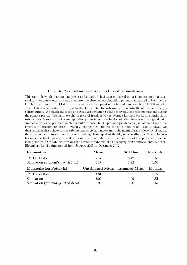
Table 15. Potential manipulation effect based on simulationsThis table shows the parameters (mean and standard deviation measured in basis points, and kurtosis)used for the simulation study, and compares the observed manipulation potential measured in basis pointsfor the three month USD Libor to the simulated manipulation potential. We simulate 20, 000 runs fora panel that is calibrated to this particular Libor rate. In each run, we simulate 16 submissions using at-distribution. We match the mean and standard deviation to the observed Libor rate submissions duringthe sample period. We calibrate the degrees of freedom to the average kurtosis based on standardizedsubmissions. We calculate the manipulation potential of three banks colluding based on the original data,simulated data and pre-manipulated simulated data. In the pre-manipulated case, we assume that threebanks have already submitted upwardly manipulated submissions on a fraction of 0.2 of all days. Wethen consider these three sets of submissions as given, and estimate the manipulation effects by changingthe three lowest observed contributions, making them equal to the highest contribution. The differencebetween the final rates with and without this manipulation is our measure of the potential effect ofmanipulation. Our data set contains the reference rate and the underlying contributions, obtained fromBloomberg for the time period from January 2005 to December 2012.

Parameters Mean Std Dev Kurtosis3M USD Libor 235 3.42 1.56Simulation (Student’s t with 8 df) 235 3.42 1.50

Manipulation Potential Untrimmed Mean Trimmed Mean Median3M USD Libor 2.01 1.61 1.28Simulation 2.02 1.69 1.51Simulation (pre-manipulated data) 1.92 1.80 1.64

63