The local economy impacts

of social cash transfers

A comparative analysis of seven

sub-Saharan countries

i

The local economy impacts of social

cash transfers

A comparative analysis of seven sub-

Saharan countries

Karen Thome

Economic Research Service (ERS), U.S. Department of Agriculture

J. Edward Taylor

University of California-Davis

Mateusz Filipski International Food Policy Research Institute (IFPRI)

Benjamin Davis Food and Agriculture Organization of the United Nations (FAO)

Sudhanshu Handa University of North Carolina at Chapel Hill

FOOD AND AGRICULTURE ORGANIZATION OF THE UNITED NATIONS

Rome, 2016

ii

The From Protection to Production (PtoP) programme, jointly with the United

Nations Children’s Fund (UNICEF), is exploring the linkages and strengthening

coordination between social protection, agriculture and rural development.

PtoP is funded principally by the United Kingdom Department for International

Development (DFID), the Food and Agriculture Organization of the United

Nations (FAO) and the European Union.

The programme is also part of the Transfer Project, a larger effort together with

UNICEF, Save the Children and the University of North Carolina, to support

the implementation of impact evaluations of cash transfer programmes in sub-

Saharan Africa.

For more information, please visit PtoP website: www.fao.org/economic/ptop

The designations employed and the presentation of material in this information product do not imply the expression of any opinion whatsoever on the part of the Food and Agriculture Organization of the United Nations (FAO) concerning the legal or development status of any country, territory, city or area or of its authorities, or concerning the delimitation of its frontiers or boundaries. The mention of specific companies or products of manufacturers, whether or not these have been patented, does not imply that these have been endorsed or recommended by FAO in preference to others of a similar nature that are not mentioned. The views expressed in this information product are those of the authors and do not necessarily reflect the views or policies of FAO. © FAO, 2016 FAO encourages the use, reproduction and dissemination of material in this information product. Except where otherwise indicated, material may be copied, downloaded and printed for private study, research and teaching purposes, or for use in non-commercial products or services, provided that appropriate acknowledgement of FAO as the source and copyright holder is given and that FAO’s endorsement of users’ views, products or services is not implied in any way. All requests for translation and adaptation rights, and for resale and other commercial use rights should be made via www.fao.org/contact-us/licence-request or addressed to copyright@fao.org. FAO information products are available on the FAO website (www.fao.org/publications) and can be purchased through publications-sales@fao.org

iii

Contents

Introduction .............................................................................................................................. 1

1. LEWIE in theory ............................................................................................................ 3

2. LEWIE in Practice .......................................................................................................... 6

2.1. Model structure ............................................................................................................ 6

2.2. Zone of Influence ......................................................................................................... 7

2.3. Model assumptions ...................................................................................................... 8

2.4. Data .............................................................................................................................. 9

2.5. LEWIE multipliers ..................................................................................................... 10

2.6. Model validation ........................................................................................................ 11

3. LEWIE findings ............................................................................................................ 12

3.1. Income multipliers ..................................................................................................... 12

3.2. Real versus nominal SCT multipliers ........................................................................ 17

3.3. Production multipliers ................................................................................................ 18

3.4. Distribution of spillovers across households ............................................................. 20

4. Conclusion ................................................................................................................. 22

References ............................................................................................................................... 23

1

Introduction

Africa has taken centre stage in the use of social cash transfer (SCT) programmes to combat

extreme poverty and vulnerability. Between 2000 and 2009, over 120 cash transfer programmes

were implemented in sub-Saharan Africa, by both governmental and non-governmental

institutions (Garcia and Moore, 2012). These programmes increasingly form part of formal

government social protection systems and range from small pilots to national, domestically

financed large-scale initiatives. These programmes vary in detail but share the same basic

approach: distributing cash transfers – usually unconditional – to individuals in ultra-poor

households and, most often, to women. Income eligibility for SCTs is typically determined

through proxy means testing and/or community-based wealth rankings. Some programmes have

additional eligibility criteria, such as the presence of orphans and vulnerable children (OVC) and

disabled adults in the household. Thus, beneficiary households are often both asset and labour

poor.

The main goal of SCT programmes is usually to improve human health and welfare outcomes in

poor and vulnerable households. However, SCTs may have productive as well as social impacts

in beneficiary households. SCTs have the immediate impact of raising purchasing power in

beneficiary households, and possibly loosening cash constraints on input purchases, financing

productive investments in credit-constrained environments and reducing income risk. They may

also affect production in non-beneficiary households through market spillovers. These spillovers

are difficult to identify experimentally because they are second-order impacts diffused over a

population that is large relative to the beneficiary population. Nevertheless the sum of these

impacts may be large, resulting in significant SCT income multipliers. That is, a dollar

transferred to a poor household may increase total income in the local economy by more than a

dollar.

By treating beneficiaries, however, SCTs also treat the local economies of which they form a

part. Beneficiaries’ spending transmits the impacts of SCT programmes to non-beneficiaries,

potentially creating production and income spillovers.

This article presents findings on the local economy impacts of seven African country SCT

programmes evaluated as part of the UN Food and Agriculture Organization’s (FAO) “From

Protection to Production” (PtoP) project.1 The countries are Ethiopia, Ghana, Kenya, Lesotho,

Malawi, Zambia and Zimbabwe (Table 1). The PtoP project has facilitated expansion of the

evaluations of SCT programmes to include productive and local-economy impacts.2 Local

economy-wide impact evaluation (or LEWIE; see Taylor and Filipski, 2014; Taylor et al., 2016)

employs simulation methods to reveal the full impact of cash transfers on local economies,

including spillovers they create to non-beneficiaries. It does this by linking agricultural

household models together into a general-equilibrium model of the local economy, in most cases

a treated village or village cluster.

1 Descriptions and reports from each of the impact evaluations can be found at the Transfer Project

(http://www.cpc.unc.edu/projects/transfer) and the PtoP (www.fao.org/economic/ptop) websites. The story of each

of the impact evaluations is told in Davis et al. (2016). 2 The results of evaluations of impacts in the beneficiary households are available on the PtoP website:

www.fao.org/economic/ptop/publications/reports/ (accessed 24 March 2015).

2

Table 1 Cash transfer programmes with LEWIE models

Country Programme Year

programme

began

Implementing

ministry

Target group

Ethiopia Tigray Social Cash

Transfer Programme

Pilot (SCTPP)

2011 Tigray Bureau of

Labour and Social

Affairs

Labour-constrained,

ultra-poor female,

elderly, or disabled

Ghana Livelihood

Empowerment

Against Poverty

(LEAP)

2008 Ministry of Gender,

Children and Social

Protection

Extreme poor with

elderly, disabled or

OVC member

Kenya Cash Transfers for

Orphans and

Vulnerable Children

(CT-OVC)

2004 Ministry of Home

Affairs, Department of

Children’s Services

Poor households with

OVC

Lesotho Child Grants

Programme (CGP)

2009 Ministry of Social

Development

Poor households with

OVC

Malawi Social Cash Transfer

Programme (SCTP) –

Expansion

2006 Ministry of Gender,

Children and Social

Welfare

Ultra-poor, labour-

constrained

Zambia Child Grant (CG)

model of the Social

Cash Transfer (SCT)

programme

2010 Ministry of

Community

Development, Mother

and Child Health

Household with a child

under 5 years old in

three poor districts

Zimbabwe Harmonized Social

Cash Transfer

(HSCT)

2011 Ministry of Public

Service, Labour and

Social Welfare

Food poor and labour-

constrained

Our LEWIE analysis finds evidence of significant spillovers, resulting in SCT income

multipliers that are considerably greater than one in most cases. Nevertheless, there is wide

variation in SCT multipliers across programmes, market settings, and household groups. Most

spillovers accrue to non-beneficiary households. Integration with outside markets shifts impacts

out of local economies, reducing local income multipliers. Local supply constraints may result in

price inflation which creates a divergence of real from nominal income multipliers for

beneficiaries as well as non-beneficiaries. The existence of income spillovers reveals that SCT

programmes have local economy impacts beyond the treated households, which could yield large

benefits for rural developments.

3

1. LEWIE in theory

A cash transfer generates spillovers if it affects households other than the intended recipients in

any way, for example, by altering their incomes, production, consumption decisions, access to

information, perceptions or even social interactions. LEWIE focuses exclusively on local

economic spillovers generated when a SCT-recipient household spends its cash transfer. These

spillovers result from general-equilibrium effects of SCTs in local economies. In economic

systems prices transmit the influences of market shocks from one actor to another. Prices are

central to LEWIE models because these models are a structural representation of how local

economies work and how they adjust to exogenous income shocks, including SCTs.

If the local economy were perfectly integrated with outside markets (i.e. if all goods were

tradable with the rest of the world), increased spending by recipient households would have no

impact on prices or on local production. Recipients would purchase goods and services from

suppliers outside the local economy at prevailing market prices. In this case, the SCT would not

create spillovers. The SCT recipients’ demand would not be large enough to affect prices in the

larger economy so prices would not convey impacts to local producers who, in turn, would not

increase production.

There are many reasons why goods in poor rural economies might not be tradable with the

outside world. Foods may be too perishable or bulky to buy or sell in distant markets. Many

services, from haircuts to prepared foods and construction, require close proximity of suppliers

to consumers. Locally-supplied goods and factors may be imperfect substitutes for those

obtainable through trade with outside markets (e.g. black versus white teff in Ethiopia or family

versus hired labour in agricultural production). Goods that are obviously tradable have a non-

tradable component. For example, the purchase of a bar of soap in a local grocery store will have

a tradable (wholesale price plus transport cost to the village) and a non-tradable (a grocery mark-

up from which wages and profits come and a possible within-village transport cost) component;

witness the substantial variation in retail prices across space. Poor roads, communications and

marketing infrastructure easily can turn what might be a tradable good – e.g. livestock or cassava

– into a nontradable, produced to supply local demand, while severely limiting labour mobility.

The existence of non-tradable goods and services with locally-determined (endogenous) prices is

a necessary condition for SCTs to generate spillovers affecting local prices and/or production.

Unlike tradable goods, which have a fixed price determined outside the local economy, markets

for non-tradable goods must clear locally (i.e. local supply must equal local demand). When

beneficiary households spend a cash transfer on non-tradable goods the local purveyors of the

goods are affected.

Spillovers create the potential for the local benefits of SCTs to exceed the amount of cash

transferred to beneficiary households. SCT multipliers are the ratio of local income gains to

transfers. A SCT multiplier that is greater than one implies positive programme spillovers.

The presence of a non-tradable good, by definition, generates spillovers, but this alone is not

sufficient to generate positive real (inflation-adjusted) SCT multipliers; there must be an

accompanying supply response. Increases in local demand from SCTs exert upward pressure on

4

local prices. The result may be expansionary (production/supply increases), or inflationary (price

increases) or a combination of the two. The expansionary response is what generates positive

local real income multipliers. Inflation, on the other hand, erodes the real value of programme

benefits. Whether and to what extent local prices actually increase depend on the elasticity of the

local supply response. Real multipliers may be less than one if supply constraints result in

substantial local price inflation.

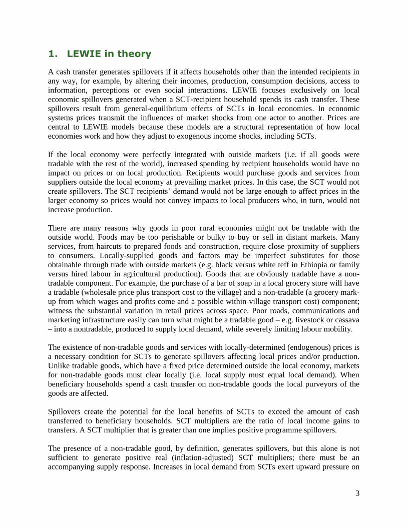
Figure 1 illustrates how SCT spillovers can create multipliers and how the size of the multiplier

depends on the local supply response (for an algebraic representation, see Filipski et al., 2015).

First consider the extreme case where local supply of a good is fixed at S2. As the SCT shifts

demand for the good from D to D’, the price increases from P1 to P2, but there is no real

expansionary effect on the economy. The quantity produced and consumed remains at Q1. This is

the worst possible outcome in terms of local economic growth because the full impact of the

SCT programme is inflationary; higher prices transfer benefits of SCTs to the owners of factors

of production while adversely affecting demanders of non-tradable consumer goods and inputs.

At the other extreme, a perfectly elastic supply response is represented by a flat supply curve, S1.

In this case, increased demand stimulates the local supply of the good, which increases from Q1

to Q2. The price does not change. Graphically, this scenario looks similar to the integrated

markets case where price is fixed exogenously and no spillovers are generated. However, when

the good is non-tradable, a perfectly elastic supply generates positive income spillovers for the

households that own the factors of production, without raising consumption costs. This is the

best possible outcome in terms of local multiplier creation because in this case the SCT is purely

expansionary and not inflationary.

In between these two extremes lie many other possibilities in which the SCT creates both local

economic expansion and inflation. Supply curve S3 depicts one of these many possibilities. The

increase in demand results in a production increase from Q1 to Q3 and in a price increase from P1

to P3. The expansionary versus inflationary impact depends on the slope of the supply curves for

non-tradables.

5

Figure 1 Illustration of possible impacts of SCT in a local market for a non-

tradable good

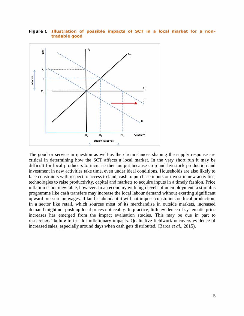
The good or service in question as well as the circumstances shaping the supply response are

critical in determining how the SCT affects a local market. In the very short run it may be

difficult for local producers to increase their output because crop and livestock production and

investment in new activities take time, even under ideal conditions. Households are also likely to

face constraints with respect to access to land, cash to purchase inputs or invest in new activities,

technologies to raise productivity, capital and markets to acquire inputs in a timely fashion. Price

inflation is not inevitable, however. In an economy with high levels of unemployment, a stimulus

programme like cash transfers may increase the local labour demand without exerting significant

upward pressure on wages. If land is abundant it will not impose constraints on local production.

In a sector like retail, which sources most of its merchandise in outside markets, increased

demand might not push up local prices noticeably. In practice, little evidence of systematic price

increases has emerged from the impact evaluation studies. This may be due in part to

researchers’ failure to test for inflationary impacts. Qualitative fieldwork uncovers evidence of

increased sales, especially around days when cash gets distributed. (Barca et al., 2015).

6

2. LEWIE in Practice

If we can simulate the local economy-wide impacts of SCTs, both nominal and real SCT

multipliers can be calculated for total income, for individual household groups and for different

production activities. LEWIE models are the basis for simulating the impacts of SCTs in the

seven programmes we examine. Their use in programme impact evaluation parallels a broad shift

from in vivo to in silico methods in the sciences (Taylor, 2015).

LEWIE models are structural general-equilibrium (GE) models that nest different groups of

households within a local economy, where they interact in markets. Each household may

participate in different income-generating activities and spend its income on goods and services

inside and outside of the local economy. Theory and empirical findings inform the design of

LEWIE, as with any simulation model. Data from baseline household surveys carried out as part

of each country’s impact evaluation reveal the production activities in which households

participate, the technologies they employ, the markets in which they transact and household

expenditure patterns. Targeted business surveys provide additional data to model production

activities for which the household surveys may not yield a sufficient sample size for econometric

estimation.

2.1. Model structure

Household groups, activities and factors form the backbone of the LEWIE model. We

aggregated household groups, activities and factors based on their significance in the local

economy and their importance to the stated goals of the SCT programmes.

Defining the household groups for LEWIE is straightforward – we follow the same criteria used

to determine households’ eligibility for SCTs. Our models include at least two households

groups: eligible households, which receive the cash transfer, and non-eligible households, which

are in the same (treated) communities but do not receive the transfer. In Kenya, we further

disaggregated the ineligible households into two groups: those not satisfying the poverty

criterion, and those satisfying the poverty criterion but not the requirement that orphans or

vulnerable children are in the household.

The LEWIE model structure is centred on the principal economic activities in which these

households participate, the households’ income sources and the goods and services on which

households spend their income. Households participate in productive activities (crop and

livestock production, retail, service and other production activities), which produce commodities

and services for sale within a given region and for sale (export) outside the region. The

productive activities use a combination of factors, including hired and family labour, land,

capital and purchased inputs (e.g. fertilizer) to produce their output. They may also purchase

commodities to use as intermediate inputs. Examples of these include local crops for food

processing, feed for livestock or imported goods for retail businesses. The activities,

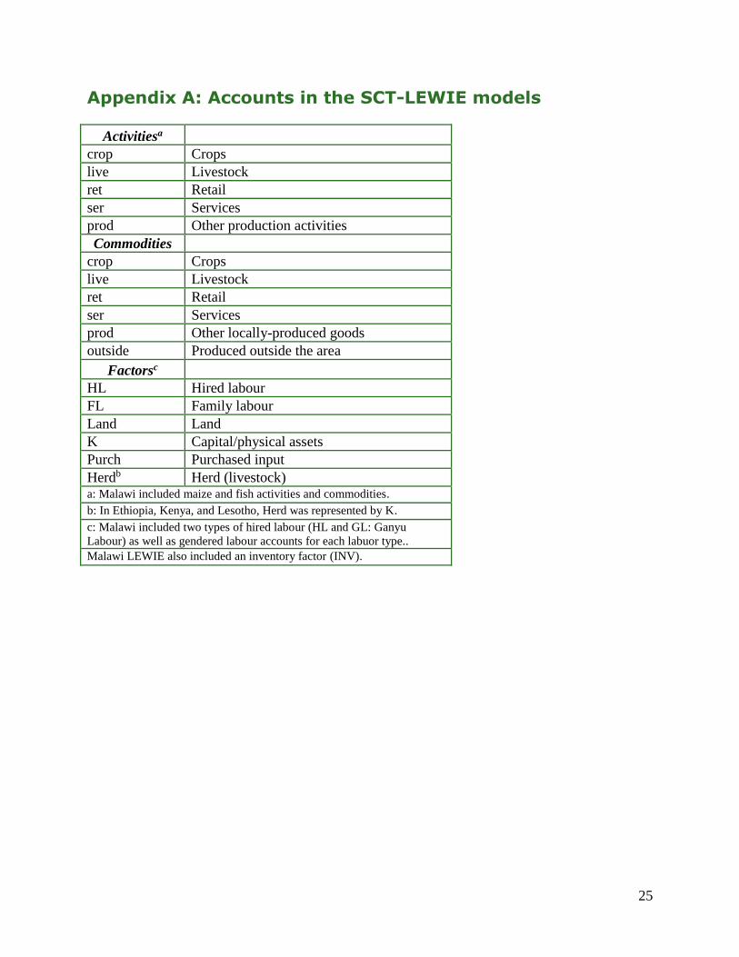
commodities and factors modelled in the SCT-LEWIEs are summarized in Appendix A.

As for expenditure, households can purchase any of the goods and services produced by local

activities or supplied by markets outside the local economy (project-area “imports”). They can

also give transfers to other households, or spend money on health care or savings. In addition to

7

income from productive activities and from selling labour or other factors, households may

receive transfers from other households and from exogenous sources, including the SCT

programme itself.

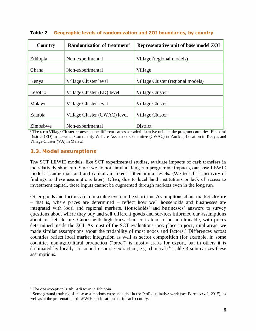
2.2. Zone of Influence

We designate a “Zone of Influence” (ZOI) as the geographic boundary of the local economy of

interest for the local economy analysis. It is the area over which LEWIE simulates the SCT

programme’s impacts and across which we calculate the SCT multipliers. In the SCT-LEWIEs

constructed for PtoP, the ZOI varies from a representative village (Ghana) to an entire district

(Zimbabwe). The choice of ZOI definition is closely linked to the programme evaluation design,

and more specifically, over how large an area we wish to document the impacts of the SCT

intervention. For example, many of the SCT programmes were randomized at the village cluster

(VC) level. In those cases it made sense to define the ZOI as a village cluster and estimate SCT

multipliers for this economic space. Table 2 presents the geographic levels at which

randomization occurred and the ZOI boundaries for each country evaluation.

In local GE analysis, goods and services fall in to two broad categories: tradable and non-

tradable. The classification of goods as tradable or non-tradable depends on where prices are

determined (we discuss the assumptions about market closure for specific items in the next

section). The prices of tradables are determined in markets outside the ZOI – thus they are

exogenous to the LEWIE. Assuming the ZOI is a price taker in larger (regional, national, or

international) markets, the prices of tradables cannot change as a result of the SCT programme.

By contrast, the prices of non-tradables are determined within the ZOI. These prices can be

affected as SCTs impact the demand for goods and services supplied within the ZOI. Local

markets and trading centres can play a role in transmitting programme impacts, and we included

these markets within our ZOIs wherever possible.

The ZOI boundaries are important for LEWIE because any purchases of goods or services

supplied by markets outside the ZOI represent leakages from the perspective of the local

economy. That is, they shift impacts from within the ZOI to markets and households outside the

ZOI. As with any kind of general-equilibrium (GE) analysis, there is no right or wrong way to

define a ZOI. Aggregate general-equilibrium models exist for regions, countries and even groups

of countries. In LEWIE, as in aggregate models, the larger the geographic area over which we

cast our net, the more potential impacts we will capture. For example, expenditures in a nearby

town do not create impacts in a village LEWIE, but they do in a district-level LEWIE that

includes both village and town. On the other hand, the wider the net is cast, the smaller the ratio

of treated to non-treated households and the less relevant the programme impacts relative to

aggregate income in the economy.

8

Table 2 Geographic levels of randomization and ZOI boundaries, by country

Country Randomization of treatmenta Representative unit of base model ZOI

Ethiopia Non-experimental Village (regional models)

Ghana Non-experimental Village

Kenya Village Cluster level Village Cluster (regional models)

Lesotho Village Cluster (ED) level Village Cluster

Malawi Village Cluster level Village Cluster

Zambia Village Cluster (CWAC) level Village Cluster

Zimbabwe Non-experimental District a The term Village Cluster represents the different names for administrative units in the program countries: Electoral

District (ED) in Lesotho; Community Welfare Assistance Committee (CWAC) in Zambia; Location in Kenya; and

Village Cluster (VA) in Malawi.

2.3. Model assumptions

The SCT LEWIE models, like SCT experimental studies, evaluate impacts of cash transfers in

the relatively short run. Since we do not simulate long-run programme impacts, our base LEWIE

models assume that land and capital are fixed at their initial levels. (We test the sensitivity of

findings to these assumptions later). Often, due to local land institutions or lack of access to

investment capital, these inputs cannot be augmented through markets even in the long run.

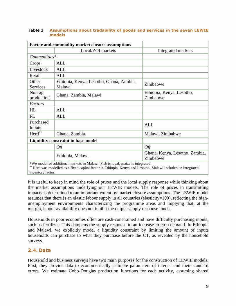
Other goods and factors are marketable even in the short run. Assumptions about market closure

– that is, where prices are determined – reflect how well households and businesses are

integrated with local and regional markets. Households’ and businesses’ answers to survey

questions about where they buy and sell different goods and services informed our assumptions

about market closure. Goods with high transaction costs tend to be non-tradable, with prices

determined inside the ZOI. As most of the SCT evaluations took place in poor, rural areas, we

made similar assumptions about the tradability of most goods and factors.3 Differences across

countries reflect local market integration as well as sector composition (for example, in some

countries non-agricultural production (“prod”) is mostly crafts for export, but in others it is

dominated by locally-consumed resource extraction, e.g. charcoal).4 Table 3 summarizes these

assumptions.

3 The one exception is Abi Adi town in Ethiopia. 4 Some ground truthing of these assumptions were included in the PtoP qualitative work (see Barca, et al., 2015), as

well as at the presentation of LEWIE results at forums in each country.

9

Table 3 Assumptions about tradability of goods and services in the seven LEWIE

models

Factor and commodity market closure assumptions

Local/ZOI markets Integrated markets

Commodities*

Crops ALL

Livestock ALL

Retail ALL

Other

Services

Ethiopia, Kenya, Lesotho, Ghana, Zambia,

Malawi Zimbabwe

Non-ag

production Ghana, Zambia, Malawi

Ethiopia, Kenya, Lesotho,

Zimbabwe

Factors

HL ALL

FL ALL

Purchased

Inputs

ALL

Herd** Ghana, Zambia Malawi, Zimbabwe

Liquidity constraint in base model

On Off

Ethiopia, Malawi Ghana, Kenya, Lesotho, Zambia,

Zimbabwe *We modelled additional markets in Malawi. Fish is local; maize is integrated. ** Herd was modelled as a fixed capital factor in Ethiopia, Kenya and Lesotho. Malawi included an integrated

inventory factor.

It is useful to keep in mind the role of prices and the local supply response while thinking about

the market assumptions underlying our LEWIE models. The role of prices in transmitting

impacts is determined to an important extent by market closure assumptions. The LEWIE model

assumes that there is an elastic labour supply in all countries (elasticity=100), reflecting the high-

unemployment environments characterizing the programme areas and implying that, at the

margin, labour availability does not inhibit the output-supply response much.

Households in poor economies often are cash-constrained and have difficulty purchasing inputs,

such as fertilizer. This dampens the supply response to an increase in crop demand. In Ethiopia

and Malawi, we explicitly model a liquidity constraint by limiting the amount of inputs

households can purchase to what they purchase before the CT, as revealed by the household

surveys.

2.4. Data

Household and business surveys have two main purposes for the construction of LEWIE models.

First, they provide data to econometrically estimate parameters of interest and their standard

errors. We estimate Cobb-Douglas production functions for each activity, assuming shared

10

technologies across all households (households have the same production function for a

particular activity). We also estimate marginal budget shares for each household group,

corresponding to a Stone-Geary utility function with no subsistence minima. The consumption

items include all the commodities produced by local activities plus outside goods, transfers to

other households and savings.

The survey data also provide initial values for all variables in the model, including production

and input levels, household demands, the value of transfers, other exogenous income and labour

market income received by each household group. The values of all of these variables differ –

often substantially – across household groups. The data sources are summarized in Appendix B

and a more detailed description of the LEWIE methodology, data and survey design process can

be found in Taylor et al. (2016).

Estimates of parameters and their standard errors, along with the starting values for all variables,

are entered onto EXCEL data input sheets (Appendix C) that interface with GAMS, where

LEWIE model resides. LEWIE uses the initial values and estimated production and expenditure

functions to create a base GE model of the project-area economy in which all actors’ incomes

equal their expenditures, and quantities supplied equal quantities demanded. The base model, in

turn, is used to simulate the impacts of the SCT programmes. The LEWIE model generates a

social accounting matrix (SAM) of the local economy as an intermediate output.

2.5. LEWIE multipliers

LEWIE multipliers are calculated by dividing the impact on the value of the outcome of interest

(income, production, etc.) by the amount transferred to eligible poor households. Income

multipliers take the total change in recipient and non-recipient household incomes and divide it

by the amount transferred, which is the cost of the SCT programme. The interpretation of the

multiplier is the amount of local income generated for each US dollar transferred to a recipient

household. If this total income multiplier exceeds one, it means that the SCT creates positive

spillovers in the local economy, such that US$1 transferred to poor households raises local

income by more than US$1. LEWIE income multipliers can also be calculated for each

household group by taking the group’s income change divided by the total cost of the SCT

programme. A LEWIE income multiplier that is greater than zero for non-beneficiary households

is evidence of positive spillovers from treated to non-treated households. A LEWIE income

multiplier that is greater than one for beneficiary households is evidence of positive feedback

effects of these spillovers on programme-eligible households.

Production multipliers are calculated as the change in production value divided by the SCT

programme cost. They represent the change in production per US$1 transferred to eligible

households. Production multipliers greater than zero are evidence of productive spillovers of

SCTs.

Unless local supply is perfectly elastic, the price of goods increases as a result of the increase in

local demand stimulated by the SCT. In this case, real (inflation-adjusted) income may be a

more accurate way to describe the SCT’s impact than nominal (non-inflation-adjusted) income.

We adjust for inflation by dividing the income change by a household-specific Laspeyres

consumer price index (CPI) generated from price change within the simulation. Real income

11

multipliers generally are smaller than nominal multipliers for SCT programmes because income

gains are partially offset by price inflation. The more elastic the local supply response, the more

nominal and real multipliers tend to converge with one another.

2.6. Model validation

Validation is always a concern in GE (as with all simulation) modelling. Econometric estimation

of production and expenditure function parameters generates standard errors along with

parameter estimates. By drawing repeatedly from all of the parameter distributions and

recreating a new base GE model from each draw, we construct confidence intervals (CIs) around

the LEWIE multipliers obtained from our simulations following Taylor and Filipski, 2014. If the

model’s parameters were estimated imprecisely this will be reflected in wider CIs around income

and production multipliers. Structural interactions within the model may magnify or dampen the

effects of imprecise parameter estimates on simulated confidence bands.

This novel Monte Carlo method of constructing confidence intervals allows us to compare

results from different modelling scenarios and test the robustness of multiplier estimates to

model assumptions. We can use confidence intervals to test for the significance of SCT impacts,

including the null hypothesis that spillover effects on production are zero and that income

multipliers are unitary – that is, a US dollar transferred to a recipient household adds no more

than a US dollar to the local economy. Similarly, we can use simulated CIs to compare real and

nominal income multipliers.

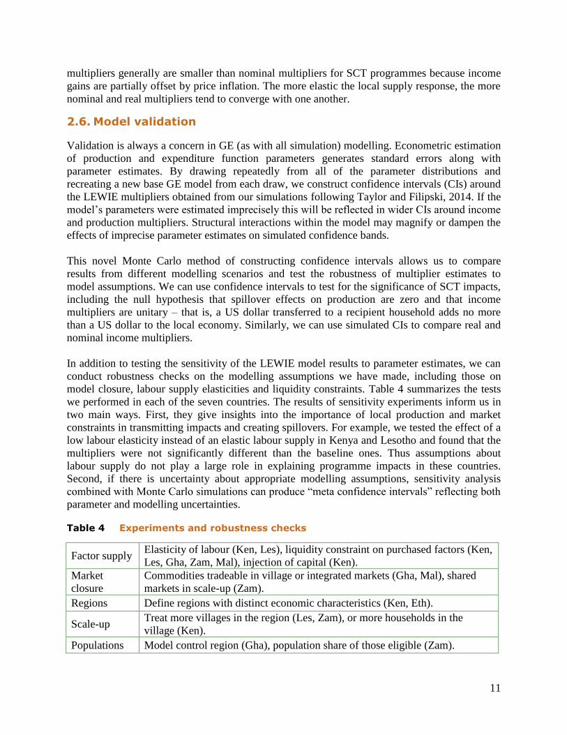
In addition to testing the sensitivity of the LEWIE model results to parameter estimates, we can

conduct robustness checks on the modelling assumptions we have made, including those on

model closure, labour supply elasticities and liquidity constraints. Table 4 summarizes the tests

we performed in each of the seven countries. The results of sensitivity experiments inform us in

two main ways. First, they give insights into the importance of local production and market

constraints in transmitting impacts and creating spillovers. For example, we tested the effect of a

low labour elasticity instead of an elastic labour supply in Kenya and Lesotho and found that the

multipliers were not significantly different than the baseline ones. Thus assumptions about

labour supply do not play a large role in explaining programme impacts in these countries.

Second, if there is uncertainty about appropriate modelling assumptions, sensitivity analysis

combined with Monte Carlo simulations can produce “meta confidence intervals” reflecting both

parameter and modelling uncertainties.

Table 4 Experiments and robustness checks

Factor supply Elasticity of labour (Ken, Les), liquidity constraint on purchased factors (Ken,

Les, Gha, Zam, Mal), injection of capital (Ken).

Market

closure

Commodities tradeable in village or integrated markets (Gha, Mal), shared

markets in scale-up (Zam).

Regions Define regions with distinct economic characteristics (Ken, Eth).

Scale-up Treat more villages in the region (Les, Zam), or more households in the

village (Ken).

Populations Model control region (Gha), population share of those eligible (Zam).

12

3. LEWIE findings

We find that all seven SCT programmes generate significant spillovers in the local economy.

The nominal programme income multipliers range from 1.27 in Malawi to 2.52 in Ethiopia-

Hintalo (Figure 2). All are significantly greater than 1.0; none of the confidence bands of the

multipliers include 1; thus, each US dollar transferred to a poor household adds more than a US

dollar to total income in the local economy. The income spillovers from SCTs equal the

multiplier minus one – that is, they range from 0.27 to 1.52 per US dollar transferred to eligible

households. This is the key result of our analysis.

The rest of this paper explores differences in multipliers across households and activities along

with the factors shaping income and production multipliers across the seven SCT programmes.

Figure 2 Nominal income multipliers with 95 percent confidence intervals for SCT

programmes in seven African countries

3.1. Income multipliers

What shapes differences in the magnitudes of multipliers across countries? The answer to this

question is complex but also important if one goal of SCT programmes is to provide a stimulus

for local economic growth. SCT multipliers illustrate the potential for cash injections to stimulate

growth in the rural economy. Ideally, we would perform a formal meta-analysis of multipliers

across project sites (Vogel, 1994); however, there is not a sufficient number of data points (sites)

to do this. We take a more descriptive approach in what follows.

Differences in multiplier magnitudes are evident both across and within county boundaries. In

Ethiopia, the SCT nominal multiplier ranges from 1.35 in Abi-Adi, an urban location, to 2.52 in

13

Hintalo, a relatively isolated rural one. Significantly, exactly the same data collection methods

and teams were used to carry out the LEWIE studies at these two locales. The same is true for

the Nyanza and Garissa regions in Kenya, for which the multiplier ranges from 1.31 to 1.84. The

size of the confidence band also varies because of differences in precision in the estimation of

expenditure and production functions across sites.

The magnitudes of SCT income multipliers are determined by a number of different factors.

Multiplier magnitudes reflect the definition of the ZOI, the nature of local production activities

and their supply response and the integration of the ZOI with outside markets. It is instructive to

compare the multipliers within Kenya and Ethiopia. Programme income spillovers begin to

accrue when a beneficiary household spends the cash. Table 5 shows eligible households’

expenditure shares on local agricultural products, at shared ZOI markets, at local businesses and

outside the ZOI5. They were estimated econometrically using data from the baseline surveys in

each country. (Ineligible households show similar patterns, but generally with more spending in

markets outside of the ZOI and less on local agriculture than eligible households).

Beneficiaries in the Nyanza region of Kenya spend 26 percent of their income outside the ZOI,

while in the pastoral Garissa, region only 7 percent of beneficiary spending is outside the ZOI.

The larger direct consumption leakage in Nyanza partially explains why the SCT multiplier is

larger in Garissa than in Nyanza. This spending has no linkage to local production and thus

cannot contribute to a local income multiplier.

Local (ZOI) versus exogenous spending by eligible households is only loosely linked to

multiplier size, however, as other mitigating factors related to the local production response to

increased demand determine the magnitude of the multiplier. For example, Hintalo and Adi-Abi,

Ethiopia, both have very low shares of beneficiary spending outside of the ZOI (1.5 percent and

0.1 percent respectively), but different SCT total income multipliers.

5 ‘Local’ spending includes purchases from store or households within a village or village cluster, depending on the

ZOI definition in a given country. Shared ZOI markets are shared across villages (or village clusters), and include

rotating markets and trading centers.

14

Table 5 Eligible household expenditure locations

Shared

ZOI

markets

Local

agriculture

Local

business Outside ZOI

Ethiopia (Abi-Adi) 0.5% 8.2% 91.1% 0.1%

Ethiopia (Hintalo) 76.7% 0.3% 22.3% 1.5%

Ghana 10.9% 20.1% 34.0% 35.0%

Kenya (Garissa) 0.8% 14.7% 77.4% 7.1%

Kenya (Nyanza) 9.9% 3.8% 60.2% 26.1%

Lesotho 22.0% 36.0% 28.9% 13.1%

Malawi 32.6% 18.7% 40.7% 8.0%

Zambia 7.5% 39.5% 49.5% 3.5%

Zimbabwe 3.7% 42.8% 39.9% 13.7%

Retail activities purchase many of the goods they sell in markets outside the ZOI at fixed prices.

However mark-ups are sensitive to local supply and demand as well as to the costs of labour and

other locally-supplied inputs. Thus retail activities have both a tradable and non-tradable

component, and retail prices may change somewhat in response to changes in local demand.

Since most of their merchandise is sourced outside the ZOI, retail activities tend to create a

major leakage for the local economy, transmitting SCT impacts elsewhere. This is good news for

production and incomes in other parts of the country, but we expect to see a negative relationship

between retail spending and local SCT multipliers. Purchased inputs, locally-produced tradables

(e.g. handicrafts) and, of course, household purchases outside the ZOI all involve tradable goods,

whose prices are determined in outside markets.

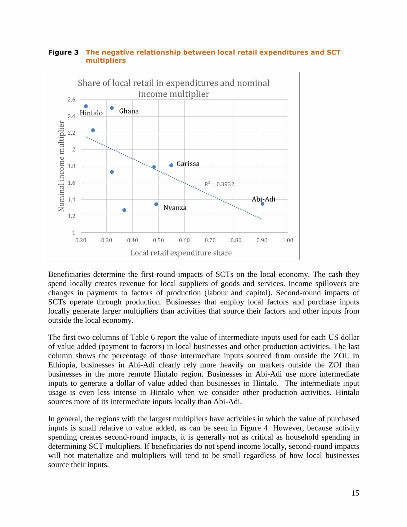
Figure 3 plots SCT nominal income multipliers against the share of retail in total local

expenditures. It is clear that there is a negative correlation between the two: the more their

budget households spend on retail, the smaller the nominal income multiplier. The two Ethiopia

sites define the extremes in this figure. Hintalo has a low retail share and large nominal SCT

multiplier, and Abi-Adi has a retail share approaching 1.0 and a correspondingly low multiplier.

Ghana has a slightly higher than expected multiplier (2.5) relative to its retail share (0.32). In

Ghana, as in the other sites, local retail businesses have large purchases of goods outside the

local economy relative to their value-added. However, other businesses rely heavily on locally-

produced inputs (Table 6). Malawi and Nyanza, Kenya, have slightly lower multipliers than

expected (1.27 and 1.34, respectively) given their retail shares (0.49 and 0.55). This is partly

because crop markets are relatively well-integrated at those sites so local spending on crops does

not have an appreciable effect on local crop production and incomes – the change in crop

demand is met largely by outside markets, not by local production.

15

Figure 3 The negative relationship between local retail expenditures and SCT

multipliers

Beneficiaries determine the first-round impacts of SCTs on the local economy. The cash they

spend locally creates revenue for local suppliers of goods and services. Income spillovers are

changes in payments to factors of production (labour and capitol). Second-round impacts of

SCTs operate through production. Businesses that employ local factors and purchase inputs

locally generate larger multipliers than activities that source their factors and other inputs from

outside the local economy.

The first two columns of Table 6 report the value of intermediate inputs used for each US dollar

of value added (payment to factors) in local businesses and other production activities. The last

column shows the percentage of those intermediate inputs sourced from outside the ZOI. In

Ethiopia, businesses in Abi-Adi clearly rely more heavily on markets outside the ZOI than

businesses in the more remote Hintalo region. Businesses in Abi-Adi use more intermediate

inputs to generate a dollar of value added than businesses in Hintalo. The intermediate input

usage is even less intense in Hintalo when we consider other production activities. Hintalo

sources more of its intermediate inputs locally than Abi-Adi.

In general, the regions with the largest multipliers have activities in which the value of purchased

inputs is small relative to value added, as can be seen in Figure 4. However, because activity

spending creates second-round impacts, it is generally not as critical as household spending in

determining SCT multipliers. If beneficiaries do not spend income locally, second-round impacts

will not materialize and multipliers will tend to be small regardless of how local businesses

source their inputs.

R² = 0.3932

1

1.2

1.4

1.6

1.8

2

2.2

2.4

2.6

0.20 0.30 0.40 0.50 0.60 0.70 0.80 0.90 1.00

No

min

al in

com

e m

ult

ipli

er

Local retail expenditure share

Share of local retail in expenditures and nominal income multiplier

Abi-Adi

Hintalo

Garissa

Nyanza

Ghana

16

Figure 4 The inverse relationship between intermediate input shares and SCT

income multipliers

Table 6 Ratios of input purchases to value added in local businesses, by source

Study site

Ratio of intermediate input value to value

added

Percent of

intermediate inputs

from outside ZOI

All business All activities All activities

Ethiopia (Abi-Adi) 0.695 0.604 0.875

Ethiopia (Hintalo) 0.486 0.028 0.721

Ghana 1.118 0.413 0.549

Kenya (Garissa) 0.728 0.587 0.820

Kenya (Nyanza) 1.052 0.992 0.941

Lesotho 2.661 1.038 0.943

Malawi 1.614 0.969 0.272

Zambia 0.850 0.693 0.250

Zimbabwe 2.775 2.043 0.471

* Value-added weighted average of retail, production, and services.

R² = 0.3351

1.2

1.4

1.6

1.8

2

2.2

2.4

2.6

0 0.2 0.4 0.6 0.8

No

min

al i

nco

me

mu

ltip

lier

Intermediate input share

Share of intermediate inputs in output

value, all activities

17

3.2. Real versus nominal SCT multipliers

According to microeconomic theory, prices transmit the impacts of SCTs through the economy.

If changes in local demand result in price increases, a given rise in nominal income will not

translate into the same increase in welfare because consumption costs will rise. Real income

multipliers take into account price changes by dividing nominal income by a local consumer

price index before and after the transfer. The changes in prices are determined within the model;

they depend on how much demand increases (or decreases) for a given commodity and the

elasticity of the supply response. Household groups may experience different rates of inflation

because they do not consume the same bundle of goods.

Figure 5 compares real and nominal income multipliers from SCTs in each of the seven

countries. In all cases, the real income multipliers are smaller than the nominal income

multipliers. This is because as SCTs increase local demand producers move up the supply curve

(see Figure 1) and this puts upward pressure on the local price. Prices of tradables are set outside

the ZOI, so they do not change; however, prices of non-tradables are determined locally and rise

unless supply is perfectly elastic. As prices change, so does the local CPI, and nominal and real

income multipliers diverge.

The gap between nominal and real multipliers varies widely from one study site to another. In

some countries, such as Malawi, the nominal and real multipliers are similar in magnitude. The

nominal income multiplier is only 8 percent higher than the real multiplier in Malawi (1.27

versus 1.18). In others, in particular Lesotho and Ghana, the real multiplier is much smaller than

the nominal one. The nominal multiplier is 64 percent higher in Lesotho (2.23:1.26) and 67

percent higher in Ghana (2.50:1.50). Gaps also vary within countries. In Ethiopia, the gap

between nominal and real multiplier is relatively small for Abi-Adi (10 percent: 1.35:1.23) but

large for Hintalo (39 percent: 2.52:1.81). In Kenya it is larger for Garissa (47 percent: 1.81:1.23)

than Nyanza (24 percent 1.34:1.08).

The main driver of the difference between the real and nominal multipliers is the elasticity of

supply of local goods. In economies that are able to easily increase the supply of a good, prices

change little and the nominal and real multipliers are relatively similar in magnitude.

18

Figure 5 Real and nominal SCT income multipliers with 90% confidence bounds

Greater integration with markets outside the ZOI lessens the potential for price inflation because

increases in local demand are met by purchasing goods outside the local economy at fixed prices.

This leads to similar real and nominal multipliers. However, outside market integration also

increases leakages, which reduce the multiplier as cash leaves the local economy through trade.

Isolation from markets (and large expenditures on non-tradable goods) can generate large

nominal income multipliers, by “trapping” cash inside the local economy. However, if the local

supply response is inelastic, market isolation also creates the potential for price inflation. The

more flexible the local supply response, the smaller the gap between nominal and real multipliers

in isolated economies.

Market integration or isolation is reflected in market closure in GE models (Table 3). Prices of

crops, livestock and services are determined locally because most basic food and service

demands are met by local production activities. Almost all local labour demand is met through

locally-supplied hired or family labour; hired-worker and family wages are thus determined in

the local economy.

3.3. Production multipliers

SCT multipliers are created by productive spillovers in local economies. Production multipliers

reveal which sectors are stimulated by the SCT. They provide insights into why some SCT

multipliers are higher than others.

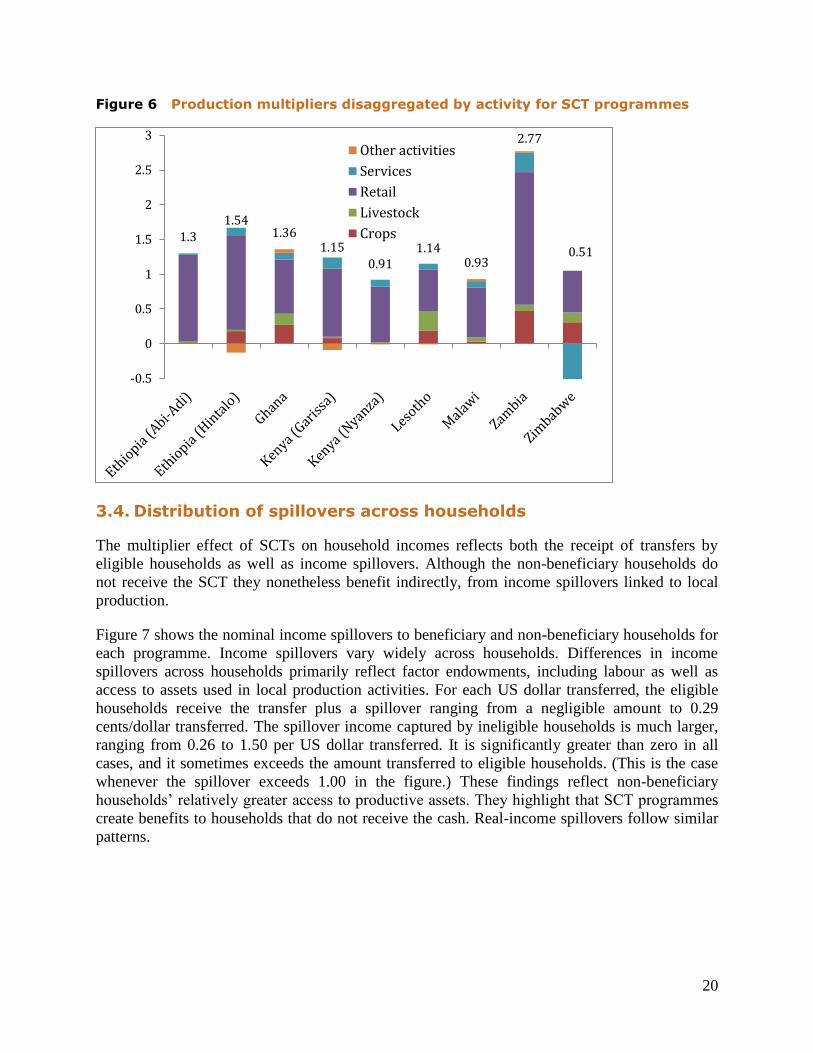
Figure 6 shows the total production multiplier for each country as well as the decomposition by

production activity. Retail production has the largest sector multiplier in every SCT-LEWIE.

This is to be expected because the largest share of expenditure by beneficiaries is on retail.

19

Crop production also benefits significantly from SCT programmes at all sites except Abi-Adi in

Ethiopia, Nyanza in Kenya and in Malawi. The absence of agricultural stimulus is expected in

Abi-Adi, an urban site. In Malawi, maize is an important local production activity; however,

maize markets are integrated to such an extent that maize prices are unresponsive to local supply

and demand. This essentially eliminates a stimulus to maize production, as do severe liquidity

constraints on crop activities. Nyanza, Kenya, is similar to the Malawi sites in that its agricultural

production is highly integrated with outside markets.

The crop production multiplier tends to be disproportionately large in areas where local crops

constitute a significant consumption share and their price is influenced by local supply and

demand. This is particularly the case in Zambia, Zimbabwe and Ghana, and, to a somewhat

lesser extent, in Hintalo, Ethiopia and in Lesotho. The livestock multiplier, predictably, is largest

in Lesotho, but it is also noteworthy in Ghana and Zimbabwe. The services multiplier is most

notable in Zambia.

Multipliers for the “other production” activity (prod) are very small or negative in all countries.

This is partially because households spend a small share of their income on these goods. In

Ethiopia, Kenya and Lesotho, other production is an integrated market, meaning that its price

does not change as a result of the SCT. In those cases the sector shrinks as households reallocate

factors in favour of producing non-tradables, whose prices rise as a result of the SCT program. In

Zimbabwe, both services and other production are integrated markets, and both of those sectors

contract as a result of the SCT. This finding is analogous to the Dutch disease phenomenon, in

which an economy’s non-tradable sectors expand but its tradable sectors contract when a new

source of external income appears.6 In Zimbabwe, services are tradable in local markets, which

lie outside the village focus of the LEWIE model there. This explains the negative impact there.

These findings offer insights into the multiplier effects of SCTs presented in Figure 3. In Ghana,

even though households spend a large share of their income on retail goods, the production

multiplier per cedi spent locally is relatively large. The opposite is true for Malawi, which has

among the lowest production multipliers among all of the sites shown in the figures.

6 Historically in the Netherlands, the new source of income was from the discovery of North Sea oil. In the present

case, it is the SCT. See Ebrahim-zadeh, C. 2003. Ebrahim-zadeh notes: “Although the [Dutch] disease is generally

associated with a natural resource discovery, it can occur from any development that results in a large inflow of

foreign currency, including a sharp surge in natural resource prices, foreign assistance, and foreign direct

investment.” In the classic Dutch disease, an inflow of foreign currency increases the exchange rate, making the

production of tradables uncompetitive with the outside world. In the case of SCTs, upward pressure on local prices

increases the real (that is, price-adjusted) exchange rate, even though the project area shares the same currency as

the rest of the country.

20

Figure 6 Production multipliers disaggregated by activity for SCT programmes

3.4. Distribution of spillovers across households

The multiplier effect of SCTs on household incomes reflects both the receipt of transfers by

eligible households as well as income spillovers. Although the non-beneficiary households do

not receive the SCT they nonetheless benefit indirectly, from income spillovers linked to local

production.

Figure 7 shows the nominal income spillovers to beneficiary and non-beneficiary households for

each programme. Income spillovers vary widely across households. Differences in income

spillovers across households primarily reflect factor endowments, including labour as well as

access to assets used in local production activities. For each US dollar transferred, the eligible

households receive the transfer plus a spillover ranging from a negligible amount to 0.29

cents/dollar transferred. The spillover income captured by ineligible households is much larger,

ranging from 0.26 to 1.50 per US dollar transferred. It is significantly greater than zero in all

cases, and it sometimes exceeds the amount transferred to eligible households. (This is the case

whenever the spillover exceeds 1.00 in the figure.) These findings reflect non-beneficiary

households’ relatively greater access to productive assets. They highlight that SCT programmes

create benefits to households that do not receive the cash. Real-income spillovers follow similar

patterns.

1.3

1.541.36

1.15

0.911.14

0.93

2.77

0.51

-0.5

0

0.5

1

1.5

2

2.5

3Other activities

Services

Retail

Livestock

Crops

21

Figure 7 Distribution of spillover of nominal income multipliers among

households

Figure 8 shows eligible households’ share of the local population and the percentage of the total

nominal spillover income they capture. Where there are relatively more eligible households, they

capture proportionately more of the spillover income. In every case, the percentage of spillovers

going to eligible households is less, however, than those households’ share of the ZOI

population. This reflects the eligibility criteria of the SCT programmes: eligible households are

targeted because they are poorer and have less access to productive assets (including labour and

land). Eligible and ineligible households’ engagement in agriculture and business activities also

determines their share of SCT spillovers.

Figure 8 The share of spillovers going to eligible households increases with

eligible households’ share of local population

22

4. Conclusion

Social cash transfers create income spillovers within local economies. Our LEWIE simulations

from seven different SCT programmes in Africa reveal that each US dollar transferred to poor

eligible households generates an additional 0.27 to 1.52 of local income. In other words, the total

income multipliers from SCTs range from 1.27 to 2.52. Most of the spillover goes to households

that are not eligible for transfers because they do not meet the poverty or other eligibility criteria

of the programmes and are positioned to respond to increased demand for local products. The

SCT programmes primarily target poor regions, in which the average income of ineligible

households is greater than beneficiary households but still relatively low. Average PPP-adjusted

baseline incomes of ineligible households range from US$300 (Ethiopia, Hintalo) to US$1,865

(Kenya, Nyanza). Our findings reveal that ineligible households as a group are indirect

beneficiaries of SCT programmes, even though they do not receive a cash transfer.

SCTs can play an important role in social protection by smoothing consumption in the poorest

and most vulnerable households. The presence of income spillovers in both eligible and

ineligible households demonstrates that SCTs can play a second role, as an economic stimulant.

Prices transmit impacts of SCTs through local economies. As local demands for goods and

services increase, an elastic supply response will result in local economic expansion, while an

unresponsive or inelastic supply may lead to price inflation that erodes the benefits to eligible

households and real-income spillovers to non-beneficiaries. An important lesson from LEWIE is

that complementary interventions aimed at lessening constraints on local production could

increase SCT multipliers and decrease the potential for inflationary impacts.

The more integrated a local economy is with outside markets, the smaller the potential

inflationary impact of SCT programmes will be, because increases in local demand are met by

outside markets instead of putting upward pressure on local prices. If prices are set in markets

outside the local economy, they cannot convey impacts to local producers, spillovers do not

materialize and SCT multipliers on the local economy tend to be lower. We can see this clearly

at the most integrated study sites, where most income is spent in retail establishments which sell

goods from outside markets. There, nominal and real SCT multipliers do not diverge greatly, but

both are lower than in places which are more isolated from outside markets.

Thanks to the spillovers they create, SCTs can play an important role in rural development

strategy. In most poor rural areas that are the target of SCT programs, the local economy is

imperfectly integrated with outside markets, and this isolation gives rise to a potential for large

multipliers, especially if there is a robust local supply response. Although integration with

outside markets leads to lower program multipliers, it can benefit households in other ways, for

example, by providing them with consumption goods at low cost.

23

References

Barca, V., Brook, S., Holland, J., Otulana, M. & Pozarny, P. 2015. Qualitative research and

analyses of the economic impacts of cash transfer programmes in Sub-Saharan Africa.

PtoP report. Rome, FAO.

Davis, B., Handa, S., Hypher, N., Winder Rossi, N., Winters, P. & Yablonski, J., eds. (in press)

From evidence to action: The story of cash transfers and impact evaluation in sub-

Saharan Africa. Oxford,UK, Oxford University Press.

Ebrahim-zadeh, C. 2013. "Back to Basics – Dutch Disease: Too much wealth managed

unwisely" In Finance and Development, a quarterly magazine of the IMF, 40 (1), March

(www.imf.org/external/pubs/ft/fandd/2003/03/ebra.htm)

Filipski, M., Taylor, J.E., Thome, K.E. & Davis, B. 2015. Effects of treatment beyond the

treated: a general-equilibrium impact evaluation of Lesotho’s cash grants programme.

Agricultural Economics 46:227-243.

Garcia, M. & Moore, C. M. T. 2012. The Cash Dividend: The Rise of Cash Transfer Programs in

Sub-Saharan Africa. Washington, DC, World Bank.

Kagin, J., Taylor, J.E., Alfani, F. & Davis, B. 2014. Local Economy-wide Impact Evaluation

(LEWIE) of Ethiopia’s Social Cash Transfer Pilot Programme . PtoP report. Rome,

FAO, and Washington, DC, World Bank.

Taylor, J.E. 2015. Cash transfer spillovers: A Local Economy-wide Impact Evaluation (LEWIE).

Policy in Focus 11(1):17-18. (Available at http://www.ipc-

undp.org/pub/eng/PIF31_The_Impact_of_Cash_Transfers_on_Local_Economies.pdf)

Taylor, J.E., Thome, K. & Filipski, M. 2014. Evaluating local general-equilibrium impacts of

Lesotho’s Child Grants Programme. PtoP report. Rome, FAO, and Washington, DC,

World Bank.

Taylor, J.E., Thome, K. & Filipski, J. Local Economy-wide Impact Evaluation of Social Cash

Transfer programmes, in Davis, B., Handa, S., Hypher, N., Winder Rossi, N., Winters, P.

& Yablonski, J., eds, From evidence to action: The story of cash transfers and impact

evaluation in sub-Saharan Africa. Oxford, UK, Oxford University Press.

Taylor, J.E., Kagin, J., Filipski, M., Thome, K & Handa, S. 2013. Evaluating general-

equilibrium impacts of Kenya's Cash Transfer Programme for Orphans and Vulnerable

Children. PtoP report. Rome, FAO, and Washington, DC, World Bank.

Taylor, J.E., Thome, K., Davis, B., Seidenfeld, D. & Handa, S. 2014. Evaluating local general-

equilibrium impacts of Zimbabwe’s Harmonized Social Cash Transfer programme

(HSCT). PtoP report. Rome, FAO.

24

Thome, K., Taylor, J.E., Davis, B., Handa, S., Seidenfeld, D. & Tembo, G. 2014. Local

Economy-wide Impact Evaluation (LEWIE) of Zambia’s Child Grant Programme.

PtoP report. Rome, FAO, and Washington, DC, World Bank.

Thome, K., Taylor, J.E., Tsoka, M., Mvula, P., Davis, B. & Handa, S. 2015. Local Economy-

wide Impact Evaluation (LEWIE) of Malawi's Social Cash Transfer (SCT) Programme.

PtoP report. Rome, FAO.

Thome, K., Taylor, J.E., Kagin, J., Davis, B., Darko Osei, R., Osei-Akoto, I. & Handa, S. 2014.

Local Economy-wide Impact Evaluation (LEWIE) of Ghana’s Livelihood Empowerment

Against Poverty (LEAP) programme. PtoP report. Rome, FAO, and Washington, DC,

World Bank.

Vogel, S. J. (1994). Structural changes in agriculture: production linkages and agricultural

demand-led industrialization. Oxford Economic Papers, 136-156.

25

Appendix A: Accounts in the SCT-LEWIE models

Activitiesa

crop Crops

live Livestock

ret Retail

ser Services

prod Other production activities

Commodities

crop Crops

live Livestock

ret Retail

ser Services

prod Other locally-produced goods

outside Produced outside the area

Factorsc

HL Hired labour

FL Family labour

Land Land

K Capital/physical assets

Purch Purchased input

Herdb Herd (livestock) a: Malawi included maize and fish activities and commodities.

b: In Ethiopia, Kenya, and Lesotho, Herd was represented by K.

c: Malawi included two types of hired labour (HL and GL: Ganyu

Labour) as well as gendered labour accounts for each labuor type..

Malawi LEWIE also included an inventory factor (INV).

26

Appendix B: Data sources for the SCT-LEWIE models

Country

Business

enterprise

surveys (BES)

Eligible hhs

(expenditures

and incomes)

Ineligible hhs

(expenditures

and incomes)

Locations and sources of

economic transactions

Ethiopia Baseline Baseline Baseline Baseline

Ghana Follow-up Baseline ISSER (2010)

(rural households)

Follow-up, locations

collected for eligible

households only, trading

partners from Zambia

Kenya Follow-up 2

(2011)

Follow-up 1

(2009) 2005 KIHBS

Follow-up 2, collected for

eligible households only

Lesotho Baseline Baseline Baseline Baseline

Malawi Baseline Baseline Baseline Baseline

Zambia Follow-up Baseline LSMS (2010)

(rural households)

Follow-up, collected for

eligible households only

Zimbabwe Baseline Baseline Baseline Baseline

27

Appendix C: Data input sheet for retail activity

Panel I Variable descriptions

Variable Type of parameter

INTD Intermediate Inputs for Activity (Value)

FD Factor Demand (Value)

beta coefficient from Cobb-Douglas production function

se standard error from Cobb-Douglas production function

acobb shift parameter from Cobb-Douglas production function

acobbse standard error on shift parameter from Cobb-Douglas production

function

alpha coefficient from expenditure function

alphase standard error from expenditure function

cmin consumption minimum

Commodity Activity/Commodity modeled (see Appendix A for definitions)

Commodity2 Commodity used as intermediate input

Factor Factor used in activity (see Appendix A for definitions)

28

Panel II Input sheets for Ethiopia and Kenya

Ethiopia Abi-Adi Ethiopia Hintalo Kenya Garissa Kenya Nyanza

Variable Commodity Commodity2 Factor HH HH HH HH HH HH HH HH HH HH

A B A B A B C A B C

INTD ret crop

INTD ret live

INTD ret ret

32468 3605793 21600 1747373 812 71 7489 11330 24883 70241

INTD ret ser

8977 997022 0 0 401 35 3700 2485 5458 15407

INTD ret prod

17161 1905826 316 25590 138 12 1276 568 1249 3524

INTD ret outside

514320 57119278 83187 6729654 6485 564 59781 72913 160139 452047

FD ret

FL 153511 17048629 44054 3563890 4775 1580 54265 22230 54668 246508

FD ret

HL 223373 24807315 127955 10351233 1720 569 19547 8007 19692 88794

FD ret

K 93012 10329673 19863 1606848 1937 641 22014 9018 22177 100001

beta ret

FL 0.327 0.327 0.230 0.230 0.566 0.566 0.566 0.566 0.566 0.566

beta ret

HL 0.475 0.475 0.667 0.667 0.204 0.204 0.204 0.204 0.204 0.204

beta ret

K 0.198 0.198 0.104 0.104 0.230 0.230 0.230 0.230 0.230 0.230

se ret

FL 0.117 0.117 0.195 0.195 0.209 0.209 0.209 0.209 0.209 0.209

se ret

HL 0.116 0.116 0.151 0.151 0.038 0.038 0.038 0.038 0.038 0.038

se ret

K 0.084 0.084 0.110 0.110 0.000 0.000 0.000

acobb ret

6.075 6.075 7.536 7.536 10.608 10.608 10.608 10.608 10.608 10.608

acobbse ret

0.774 0.774 1.203 1.203 0.258 0.258 0.258 0.258 0.258 0.258

alpha ret

0.903 0.958 0.219 0.014 0.550 0.695 0.841 0.492 0.631 0.365

alphase ret

0.012 0.006 0.013 0.003 0.028 0.042 0.014 0.013 0.015 0.034

cmin ret 0 0 0 0 0 0 0 0 0 0

29

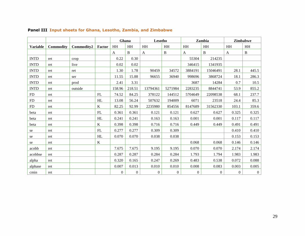
Panel III Input sheets for Ghana, Lesotho, Zambia, and Zimbabwe

Ghana Lesotho Zambia Zimbabwe

Variable Commodity Commodity2 Factor HH HH HH HH HH HH HH HH

A B A B A B A B

INTD ret crop

0.22 0.30

55304 214235

INTD ret live

0.02 0.02

346415 1341935

INTD ret ret

1.30 1.78 90459 34572 3884191 15046491 28.1 445.5

INTD ret ser

11.55 15.88 96655 36940 998696 3868724 18.1 286.3

INTD ret prod

2.41 3.31

3687 14284 0.7 10.5

INTD ret outside

158.96 218.51 13794361 5271984 2283235 8844741 53.9 855.2

FD ret

FL 74.52 84.25 378122 144512 5704649 22098538 68.1 237.7

FD ret

HL 13.08 56.24 507632 194009 6071 23518 24.4 85.3

FD ret

K 82.25 92.99 2235980 854556 8147689 31562330 103.1 359.6

beta ret

FL 0.361 0.361 0.121 0.121 0.627 0.627 0.325 0.325

beta ret

HL 0.241 0.241 0.163 0.163 0.001 0.001 0.117 0.117

beta ret

K 0.398 0.398 0.716 0.716 0.449 0.449 0.491 0.491

se ret

FL 0.277 0.277 0.309 0.309 0.410 0.410

se ret

HL 0.070 0.070 0.038 0.038 0.153 0.153

se ret

K

0.068 0.068 0.146 0.146

acobb ret

7.675 7.675 9.195 9.195 0.070 0.070 2.174 2.174

acobbse ret

0.287 0.287 0.284 0.284 1.793 1.794 1.983 1.983

alpha ret

0.320 0.165 0.247 0.269 0.483 0.538 0.072 0.088

alphase ret

0.007 0.013 0.010 0.010 0.008 0.083 0.003 0.005

cmin ret 0 0 0 0 0 0 0 0

30

Panel IV Input sheet for Malawi

Malawi

Variable Commodity Commodity2 Factor HH HH

A B

INTD ret zoi

698 36019

INTD ret outside

454 23418

INTD ret crop

4 227

INTD ret maize

1 63

INTD ret live

101 5191

INTD ret fish

0 26

INTD ret ser

84 4334

INTD ret ret

85 4364

FD ret

FLF 100 2470

FD ret

FLM 780 19326

FD ret

HLF 2 55

FD ret

HLM 3 69

FD ret

K 72 2431

FD ret

INV 374 9262

beta ret

FLF 0.040 0.040

beta ret

FLM 0.313 0.313

beta ret

HLF 0.001 0.001

beta ret

HLM 0.001 0.001

beta ret

K 0.084 0.084

beta ret

INV 0.150 0.150

se ret

FLF 0.072 0.072

se ret

FLM 0.079 0.079

se ret

HLF

se ret

HLM

se ret

K 0.029 0.029

se ret

INV 0.047 0.047

acobb ret

8.560 8.560

acobbse ret

0.449 0.449

alpha ret

0.368 0.401

alphase ret

0.012 0.013

cmin ret 0 0

Food and Agriculture Organization of the United Nations (FAO) di

Viale delle Terme di Caracalla

00153 Rome, Italy

The From Protection to Production (PtoP) programme, jointly implemented by FAO and UNICEF, is contributing to the generation of solid evidence on

the impact of cash transfer programmes in Sub-Saharan Africa.

PtoP seeks to understand the potential effects of such programmes on

food security, nutrition, as well as their contribution to rural livelihoods and economic growth at household and community levels in Ethiopia,

Ghana, Kenya, Malawi, Lesotho, Zambia and Zimbabwe. 7

7This publication has been produced with the assistance of the European Union. The contents of this publication are the sole responsibility of FAO and can in no way be taken to reflect the views of the European Union.

I5375E

/1/0

2.1

6