HETEROGENEOUS IMPACTS OF CONDITIONAL CASH TRANSFERS: EVIDENCE FROM …ftp.iza.org/dp3653.pdf · 2008-08-21 · IZA Discussion Paper No. 3653 August 2008 ABSTRACT Heterogeneous Impacts

IZA DP No. 3653

Heterogeneous Impacts of Conditional Cash Transfers:Evidence from Nicaragua

Ana C. Dammert

DI

SC

US

SI

ON

PA

PE

R S

ER

IE

S

Forschungsinstitutzur Zukunft der ArbeitInstitute for the Studyof Labor

August 2008

Heterogeneous Impacts of

Conditional Cash Transfers: Evidence from Nicaragua

Ana C. Dammert Carleton University

and IZA

Discussion Paper No. 3653 August 2008

IZA

P.O. Box 7240 53072 Bonn

Germany

Phone: +49-228-3894-0 Fax: +49-228-3894-180

E-mail: [email protected]

Any opinions expressed here are those of the author(s) and not those of IZA. Research published in this series may include views on policy, but the institute itself takes no institutional policy positions. The Institute for the Study of Labor (IZA) in Bonn is a local and virtual international research center and a place of communication between science, politics and business. IZA is an independent nonprofit organization supported by Deutsche Post World Net. The center is associated with the University of Bonn and offers a stimulating research environment through its international network, workshops and conferences, data service, project support, research visits and doctoral program. IZA engages in (i) original and internationally competitive research in all fields of labor economics, (ii) development of policy concepts, and (iii) dissemination of research results and concepts to the interested public. IZA Discussion Papers often represent preliminary work and are circulated to encourage discussion. Citation of such a paper should account for its provisional character. A revised version may be available directly from the author.

mailto:[email protected]

IZA Discussion Paper No. 3653 August 2008

ABSTRACT

Heterogeneous Impacts of Conditional Cash Transfers: Evidence from Nicaragua

In the last decade, the most popular policy tool used to increase human capital in developing countries has been the conditional cash transfer program. A large literature has shown significant mean impacts on schooling, health, and child labor. This paper examines heterogeneous effects using random-assignment data from the Red de Proteccion Social in rural Nicaragua. Using interactions between the targeting criteria and the treatment indicator, estimates suggest that children located in more impoverished localities experienced a larger impact of the program on schooling in 2001, but this finding is reversed in 2002. Estimated quantile treatment effects indicate that there is considerable heterogeneity in the impacts of the program on the distribution of food expenditures, as well as total expenditures. In particular, households at the lower end of the expenditure distribution experienced a smaller increase in expenditures. This paper also presents evidence of the rank invariance assumption to help clarify the interpretation of the quantile treatment effect in the development literature context. JEL Classification: O15, I38 Keywords: Nicaragua, conditional cash transfers, quantile treatment effect Corresponding author: Ana C. Dammert Department of Economics Carleton University Loeb B-846 1125 Colonel by Drive Ottawa, Ontario, K1S 5B6 Canada E-mail: [email protected]

mailto:[email protected]

2

I. INTRODUCTION

The most popular policy tool used in the last decade in developing countries to

increase human capital has been the conditional cash transfer program, which provides cash

payments to households conditional on regular school attendance and visiting health clinics.

Many governments implemented experimental frameworks to assess the impacts of

conditional cash transfers on employment, schooling, and health among poor eligible

households (PROGRESA in Mexico and PRAF in Honduras, among others). Though

conditional cash transfers have achieved quantified success in reaching the poor and bringing

about short-term improvements in consumption, education, and health (Schultz 2004; Gertler

2004; Rawlings and Rubio 2003), most of the literature has focused on mean impacts. As

Heckman, Smith, and Clements (1997) point out, however, judgments about the “success” of

a social program should depend on more than the average impact. For example, it may be of

interest to investigate whether social programs have differential effects for any subpopulation

defined by covariates, for example gender effects, or whether there is heterogeneity in the

effect of treatment. Knowledge of whether a program’s impacts are concentrated among a

few individuals is important for the effectiveness of the program in reaching its target

population.

This paper contributes to the small but growing literature on the estimation of

heterogeneous effects of conditional cash transfers in developing countries. This type of

program has received a great deal of attention among policymakers, influencing adoption of

new policies in Latin and Central America. The assessment of heterogeneous impacts is done

with a unique data set from a social experiment in Nicaragua designed to evaluate a

conditional cash transfer program targeted to poor rural households, the Red de Proteccion

Social (hereafter RPS) or Social Safety Net. The analysis takes advantage of the random

assignment of localities to treatment and control groups so that program participation is not

3

correlated in expectation with either observed or unobserved individual characteristics and

outcome differences provide an unbiased estimate of the true mean impact of the program.

The purpose of this paper is to investigate the degree of heterogeneity in program impacts of

the RPS program for education, health, and nutrition in Nicaragua. This paper explores the

heterogeneity of impacts as a function of observable characteristics (age, gender, poverty, and

household head characteristics) and the criteria used by the RPS to select beneficiaries. This

paper also investigates the overall heterogeneity of program impacts using quantile treatment

effects (QTE), which allows us to test whether conditional transfers lead to larger or smaller

changes in some parts of the outcome distribution.

This paper adds to the existing literature in several ways. First, the existing literature

on conditional cash transfers focuses on mean impacts, in the full sample and in demographic

subgroups. This paper goes beyond mean impacts and interaction variables and tests whether

there are heterogeneous impacts of conditional cash transfers on the distribution of

expenditures. Conditional cash programs, such as the RPS, have differential effects on

household behavior given that transfers affect regular school attendance and health visits. For

example, the school cash transfer is conditional on regular attendance of children age 7 to 13

years who have not yet completed the 4th

grade. For households with children age 7 to 13

years who have not completed fourth grade and are not attending school, the program has

income effects of the cash transfer and substitution effects of a lower price of schooling

driven by the attendance requirement. Some households may have to bear the cost of

children’s foregone labor earnings due to the implicit reduction in labor time, in which case

the impact on household expenditures may be negative if the RPS transfer does not make up

for losses in income from market work. The monetary transfer received to buy food (or food

cash transfer), however, has a positive effect on household expenditure. The net effect on

expenditures could be positive or negative. Conditional cash transfers have differential effects

4

based on whether the household is meeting the requirements prior to the implementation of

the program. Knowing more about this heterogeneity is relevant to anti-poverty policies

(Ravallion, 2005).

Second, the literature on QTE has been limited mostly to the US context. Recent

papers have used QTE to assess the impacts of training programs on labor outcomes such as

Heckman, Smith, and Clements (1997); Black, Smith, Berger, and Noel (2002); Abadie,

Angrist, and Imbens (2002); and Firpo (2007). Bitler, Gelbach, and Hoynes (2005, 2006)

examine the impact of welfare reform experiments on earnings and total income. Overall, the

main finding is that variation in the impact of treatment across persons is an important aspect

of the evaluation problem. To the best of my knowledge, Djebbari and Smith’s (2005) study

represents the first to analyze heterogeneous impacts of social programs in a developing

country using QTE.

Third, QTE corresponds, for any fixed percentile, to the horizontal distance between

two cumulative distribution functions. Under the rank preservation assumption, QTE can be

interpreted as the treatment effect for individuals at particular quantiles of the control group

outcome distribution or the treatment effect for each quantile in the distribution (Bitler,

Gelbach, and Hoynes, 2005). Without the rank preservation assumption, QTE represents how

various quantiles of the outcome distribution change in the treatment and control groups, but

we cannot make inference on the impact on any particular person. This paper presents

evidence of rank invariance in the RPS context to help clarify the interpretation of the QTE

impacts for the development literature.

The main results show that impact estimates vary among the eligible population. From

the analysis on subgroups, the estimates show that boys experienced a larger positive impact

of the program on schooling and a negative impact on the probability of engaging in labor

activities and hours worked. The estimates also show that older children experienced a

5

smaller impact of the program on schooling and participation in labor activities. There are

also differential impacts by whether the child is living with a male head of household and

with education of the head of household. To assess the effectiveness of the targeting criteria,

the analysis considers the interaction between the treatment indicator and marginality index

and household per capita expenditures, separately. The main results show that children

located in more impoverished areas experienced a larger impact on schooling and a smaller

impact on working hours.

From the QTE analysis, the estimates suggest that the positive program impact in per

capita food expenditures and total per capita expenditures is smaller for households who are

in the lower tail of the expenditure distribution. The estimates show that program impacts are

larger for households who had lower levels of food shares prior to the program. These

findings are consistent with the theoretical prediction that treatment effects on expenditures

are lower for households whose costs of complying with the program requirements are

highest. Tests of the null hypothesis of constant treatment effects reveal that these findings

could not have been revealed using mean impact analysis. Finally, joint tests of rank

preservation show that the distributions of observable characteristics in all ranges of the

expenditures distribution do not vary significantly between the treatment and control group.

The rest of the paper is organized as follows. Section II presents the RPS Program and

data and Section III outlines the theoretical framework. Section IV outlines the empirical

strategy and this is followed by a discussion of the empirical results in Section V. Section VI

concludes.

6

II. THE RPS PROGRAM

II.1 Program Structure and Benefits

Nicaragua is a lower-middle income country. With an estimated per capita GDP of

US$817 in 2004, Nicaragua remains the second poorest country in the Latin America and

Caribbean region after Haiti. In 2000, the Nicaraguan government implemented the Red de

Proteccion Social or Social Safety Net to encourage educational attainment and help

impoverished households in rural areas. Phase I of the program started with a budget of

US$11 million, representing approximately 0.2 percent of Nicaragua’s GDP (Maluccio and

Flores 2005). With financial assistance from the Inter-American Development Bank and the

government of Nicaragua, the RPS program was expanded in 2002 with a US$20 million

budget for coverage for an additional three years. The RPS program provided benefits

conditional on school attendance and health checkups, where participants were identified

using a detailed targeting process aimed at reaching poor people in rural areas.

For Phase I of the RPS, the Government of Nicaragua selected the departments of

Madriz and Matagalpa from the northern part of the Central Region. This selection was based

on the departments’ ability to implement the program in terms of institutional and local

government capacity, high poverty levels within the communities, and proximity to the

capital of Nicaragua. In 1998, approximately 80 percent of the rural population in Madriz and

Matagalpa was poor and half was extremely poor.

Targeting of poor households was implemented at the RPS headquarters in two

stages: (1) officials selected six municipalities within these two departments based on criteria

similar to those used at the department level, (2) officials selected eligible comarcas within

the selected municipalities based on the marginality index constructed from the 1995

National Population and Housing Census. Comarcas (hereafter called localities) are

administrative areas within municipalities including between one and five small communities

7

averaging 100 households each. This marginality index used locality-level information on the

illiteracy rate of persons over age 5, access to basic infrastructure (running water and

sewage), and average family size. The higher the value of the marginality index, the more

impoverished the area. Out of 59 localities, 42 eligible rural localities were identified as

having a high or very high marginality index and thus pre-selected for the program.1

Program benefits are conditional income transfers composed of (Table 1):

1. Each eligible household received money to buy food (called the food cash transfer)

every other month. In order to receive this transfer, a household member (typically the

mother) is required to attend educational workshops and bring their children under the

age of five for preventive health care appointments (including vaccinations and

growth monitoring). Children younger than age two were seen monthly and those

between age two and five, every other month. In September 2000, the food transfer

was US$224 a year, representing 13 percent of total annual household expenditures in

beneficiary households before the program.

2. Contingent on enrollment and regular attendance, each household with children age 7

to 13 who had not completed the fourth grade of primary school received a fixed cash

transfer every other month. 2,3

In addition, for each eligible child in the household

enrolled in school, the household received an annual lump sum transfer for school

supplies and uniforms (called the school supplies transfer).4 In September 2000, the

school attendance transfer and the school supplies transfer were US$112 and US$21,

respectively.

To enforce compliance with program requirements, beneficiaries did not receive the

transfer if they failed to carry out the conditions previously described. Less than 1 percent of

households were expelled during the first two years of delivering transfers, though 5 percent

8

voluntarily left the program, e.g., by dropping out or migrating out of the program area

(Maluccio and Flores, 2005).

II.2 The Experimental Design and Data

The evaluation design is based on an experiment with randomization of localities into

treatment and control groups. One-half of the 42 localities were randomly selected into the

program. The selection was done at a public event in which the localities were ordered by

their marginality index scores and stratified into seven groups of six localities each. Within

each group, randomization was achieved by blindly drawing one of six colored balls without

replacement; the first three were selected in the program and the other three in the control

group.5

All households in selected localities are interviewed before and after the random

assignment. The evaluation dataset consists of panel-data observations for 1,359 households

over 3 rounds of survey (baseline: September 2000, follow-ups: October 2001 and October

2002). Surveys at the individual and household level collected information on socioeconomic

and demographic characteristics such as parental schooling, labor market outcomes, health,

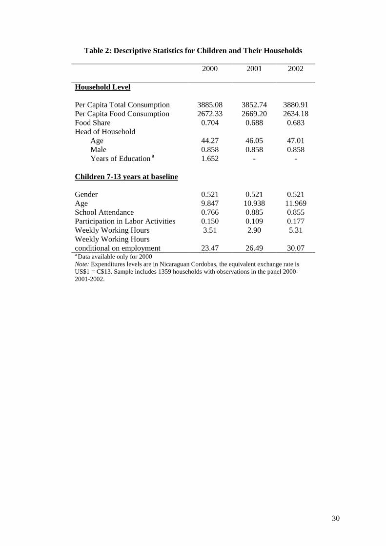
nutrition, and attributes of the physical infrastructure of the household, among others.6 Table

2 presents descriptive statistics for each year. Prior to the program, the mean per capita

consumption was 3885 Nicaraguan Cordobas (hereafter C$) or about US$298.9 a year, with

70 percent allocated to food consumption. Table 2 also shows that 77 percent of children

aged 7 to 13 years attend school and 15 percent participate in labor activities for an average

of 23.5 hours per week.

The randomization is at the locality level rather than at the household or individual

level. One reason for doing the random assignment at the locality level was to avoid spillover

effects between treated and untreated individuals in the same locality. This was part of the

9

motivation for doing the random assignment at the village level in the PROGRESA

evaluation as well.7 Assignment by randomization at the locality level ensures the treatment

and control groups are similar on average in terms of observable and unobservable

characteristics. There is a chance, however, of observing some non-randomness in terms of

differences between localities selected for the control and treatment groups at the household

level prior to the program, since estimates of average quantities are more reliable with large

sample sizes and the sample subject to randomization is small (42 localities) (Behrman and

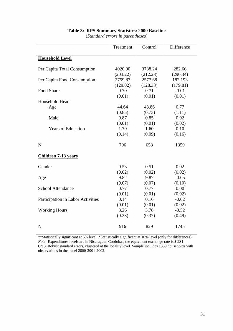
Todd, 1999). Table 3 shows t-tests of the equality of means at the household and individual

level. Main results show that the majority of variables measured prior to the random

assignment do not differ between the treatment and control groups, which suggest that the

sample is well balanced across these groups.8

III. THEORETICAL FRAMEWORK

This section outlines a model of household decision-making in the presence of

conditional cash transfers in order to get a better understanding of potential heterogeneous

impacts of the RPS program. The model is based on Skoufias and Parker (2001) and Djebbari

and Smith (2005). The analysis begins first by considering household time allocation in the

absence of the conditional cash transfer. Neoclassical models of household decision-making

are commonly employed in this analysis. In this framework, parents make decisions about the

allocation of a child’s schooling time, the time of other household members, and the purchase

of goods and services. Parents will invest in each child’s schooling up to the point where the

marginal costs of a child’s time in school equal the marginal benefits considering the

opportunity cost of schooling, which is the foregone earning from work.

The opportunity cost of children’s time is likely to vary with observed characteristics.

For example, it is expected to see gender and age differences in child labor if boys and girls

10

have different returns to education or older children have a comparative advantage in the

labor market. It is important to note that the RPS does not provide higher payments for

female enrollment in school as in PROGRESA where the main idea was to equalize the

incentive for girls in the face of higher wages, on average, for boys in the labor market. Girls

in secondary school received slightly higher subsidies (by about $2 per month) than boys in

Mexico.

The existing literature on heterogeneity of treatment effects predominantly looks at

the impact of the program as if it varies with observed characteristics or subgroups of the

population. In the case of conditional cash transfers, other papers have found evidence of

differential impacts on schooling and child labor for girls vs. boys, and primary school-age

children vs. secondary school-age children, and by socioeconomic status (for example

Maluccio and Flores (2005) for RPS; Skoufias (2005) for PROGRESA; Schady and Araujo

(2006) in Ecuador; Behrman, Sengupta, and Todd (2005) for PROGRESA; Filmer and

Schady (2008) for Cambodia; Djebbari and Smith (2005) for PROGRESA).

The conditionality of the transfer has important effects on household behavior as well.

The monetary school and food cash transfers are linked to the school attendance of children

aged 7 to 13, participation in health clinics, and other criteria. If they were not conditioned,

transfers would act as a pure income effect. Conditionality of the transfers results in changes

in the marginal cost of investment in schooling. If children participate in the program with

full compliance of the requirements, time devoted to schooling changes: children now receive

transfers for attendance and school supplies but lose wages for the extra time the child

devotes to schooling. What matters is the ratio of the child’s wage and the marginal increase

in income due to the transfer.

11

Participation and compliance with the RPS program might affect household behavior as

follows: 9

Households with no children in the targeted age ranges or with children under age 5

(but without children aged 7 to 13 who have not completed the fourth grade) receive

the food cash transfer. These transfers will have a pure income effect and it is

expected that these households will have higher expenditures after the program.

Households with children aged 7 to 13 years old who have completed fourth grade at

primary school and are attending school without the program will be eligible to

receive food transfers but not school transfers. Food cash transfers will have a pure

income effect and it is expected that these households will have higher expenditures

after the program.

Households with children aged 7 to 13 years, who have not completed fourth grade

but are attending school even without the program, are eligible for both the food and

school cash transfers. These transfers will have a pure income effect and it is expected

that these households will have higher expenditures after the program.

For households with children aged 7 to 13 years who have not completed fourth grade

and are not attending school without the program, the RPS program combines the

income effect of the school transfer with the substitution effect of a lower price of

schooling driven by the attendance requirement. Some households may have to bear

the cost of children’s foregone labor earnings due to the implicit reduction in labor

time, in which case the impact on household expenditures may be negative if the RPS

transfer does not make up for losses in income from market work. Thus the program

impact on household expenditures may be negative. At the same time, the food cash

transfer will have an income effect. The net effect of the school and food transfer on

expenditures could be positive or negative for these households.

12

In sum, the predicted effect on expenditures is heterogeneous. At the top of the

expenditures distribution, or the richest households among the eligible ones, households are

meeting or almost meeting program requirements prior to the program and thus, the impacts

will be larger. For some part of the bottom of the expenditures distribution are located

households who are not meeting the requirements (e.g. children are not going to school the

minimum required time) and for which the cost of participation is the highest (children’s

contribution is significant), for them the program impacts could be positive or negative.

These households are likely to be the ones who rely greatly on child labor. As Basu and

Van’s (1998) seminal model shows a household will send children to work if adult income or

family income from non-child labor sources becomes very low. In between these extremes,

the effect of the program depends on whether the child is attending school the minimum

required time or not. The extent to which the program has a significant impact on different

parts of the expenditure distribution can only be determined through empirical analysis.

IV. EMPIRICAL STRATEGY

Let 1Y denote the potential outcomes of interest in the presence of treatment, 1iT ,

and 0Y without treatment 0iT . Each individual experiences only one of these treatment and

untreated outcomes, thus the critical objective is to establish a credible comparison group or a

group of individuals who in the absence of the program would have had outcomes similar to

those who were exposed to the program. In this paper the treatment and control group are

randomly selected, so that program participation is not correlated in expectation with either

observed or unobserved individual characteristics and outcome differences provide an

unbiased estimate of the true mean impact of the program.10

What we are interested is in estimating the expected average effect that the RPS

program have on different outcomes, or the average treatment effect (ATE),

13

1 0 ( )ATE E Y Y . The literature also focuses on the mean impact of treatment on the treated

(ATET), given by 1 0 ( | 1)ATET E Y Y T . Under the assumptions of no equilibrium

effects and no randomization bias, the randomized experiment identifies the ATET (Djebbari

and Smith, 2008).

I.V.1 Impacts at the Subgroup Level

The first method generates impact estimates that vary among the eligible population

by considering variation in impacts as a function of observable characteristics through the

interaction of the treatment indicator in equation (1) with a variety of individual and locality

characteristics as follows:

0 1 2 3* *i i i i i i iy C T T C X , (1)

where iy is some outcome measure,

iC is the characteristic of interest, iT is a dummy

variable representing whether the locality was randomly assigned to the treatment or control

group, and *i iT C represent the interactions between the characteristics and the treatment

indicator.

The interpretation of the coefficients is as follows: for example, in the specification

that tests for heterogeneous impacts by gender, iC is a dummy variable equal to one if the

child is male, the coefficient 1is an estimate of the difference in the outcome between boys

and girls, the RPS effect for girls is given by2, the corresponding effect for boys is given by

the sum of the coefficients2 3

. If 3is statistically significant different from zero, there is

evidence of heterogeneity of treatment effects by gender.

iC also includes characteristics of the head of household and locality. I also use a

criterion used by PRS to select beneficiaries, the locality marginality index. Program officials

using data from the 1995 Nicaraguan Household Survey, collected prior to the program,

14

constructed this index. Following the analysis in Djebbari and Smith (2005) for Mexico, the

impact of conditional cash transfers is expected to be largest for households living in more

impoverished localities as defined by the marginality index. If the targeting mechanism is

efficient, then households in the most marginal localities get a greater program impact than

less marginal places. Equation (1) also controls for other baseline household and individual

characteristics (iX ) to take into account any differences that were present despite

randomization and to increase the precision of the coefficient estimates. The standard errors

are clustered at the locality level.

I.V.2 Quantile Treatment Effects

The method described in the previous section emphasized differences in means. While

the mean is important, comparisons of means only account for shifts in the central tendency

of a distribution. For many questions, knowledge of distributional parameters is required; for

example, the proportion that benefit from treatment, the proportion that gain at least a fixed

amount, or the quantiles of treatment effect (Heckman, Smith, and Clements, 1997). One

particular feature of interest in the RPS context is the behavior at the left tail of the

consumption distribution, as this measures consumption of those households that most likely

are not meeting the requirements (children are not going to school the minimum required

time) and for which the cost of participation is the highest (children’s contribution is

significant). In order to capture responses across the entire distribution of consumption, the

second econometric method uses the QTE approach.

Most of the existing literature on QTE is based on social experiments in employment,

training and welfare programs in the US. Heckman, Smith, and Clemens (1997), find strong

evidence that heterogeneity is an important feature of impact distributions using experimental

data from the National Job Training Partnership Act Study. Black, Smith, Berger, and Noel

15

(2002), using experimental data from the Worker Profiling and Reemployment Services

program, find that the estimated impact of treatment varies widely across quantiles of the

outcome distributions. The pattern of impacts suggests that the treatment has its largest effect

on persons whose probability of unemployment insurance benefit exhaustion without

treatment would be of moderate duration. In evaluating the economic effects of welfare

reform, Bitler, Gelbach, and Hoynes (2005, 2006) find strong evidence against the common

effect assumption using experimental data from the Connecticut’s Job First Waiver program

and the Canadian Self-Sufficiency Project. Their estimates suggest substantial heterogeneity

in the impact of welfare reform on earnings and total income, which is consistent with the

predictions from the static labor supply model.

Let 1Y and

0Y denote the outcome of interest in the treated and control states with

corresponding cumulative distribution functions 1 1( ) Pr[ ]F y Y y and

0 0( ) Pr[ ]F y Y y .

Let denote the quantile of each distribution

( ) inf{ : ( ) }, T 0,1Ty T y F y , (2)

where “ inf ” is the smallest attainable value of y that satisfies the condition stated in the

braces. The quantile treatment effect at quantile is defined as ( 1) ( 0)QTE y T y T .

For example, suppose that y represents family income in a given year, 0.25y is that level of

income for households in the treatment (control) group such that 25 percent of treatment

(control) households have income below it. 0.25

QTE is given by the difference between the

income of households in the 25th

percentile of the treated distribution and the 25th

percentile

of the control distribution.

The impact estimate for a given quantile is the coefficient on the treatment

indicator from the corresponding quantile regression as follows:

( | ) ( ) ( ) , (0,1)iiQ y T T , (3)

16

where ( | )iQ y T denotes the quantile of expenditures conditional on treatment.11

As presented above in table 2, the RPS sample is well balanced and there are few

statistical differences in the observable characteristics in the two groups. To correct for any

differences not accounted for by the randomization of localities into treatment and control

groups and to obtain more precise estimates, I have included covariates as in Djebbari and

Smith (2005).12

The vector of control variables includes characteristics of the head of

household (age, education, gender, employment) and household demographic composition.13

The advantage of the QTE approach relative to the common effect model is that the impact of

the program on different quantiles of the outcome distribution does not have to be constant.

Note that although average differences equal differences in averages, the treatment

effect at quantile is not the quantile of the difference (Y1- Y0). The QTE corresponds, for

any fixed percentile, to the horizontal distance between two cumulative distribution

functions. Under the rank preservation assumption, QTE can be interpreted as the treatment

effect for individuals at particular quantiles of the control group outcome distribution or the

treatment effect for the person located at quantile in the distribution (Heckman, Smith and

Clements 1997; Bitler et al. 2005). Without the rank preservation assumption, QTE

represents how various quantiles of the outcome distribution change in the treatment and

control groups, but we cannot make inference on the impact on any particular person.

Rank preservation across treatment status is a strong assumption as it requires that the

rank of the potential outcome for a given individual would be the same under treatment as

under non-treatment. There are two ways to deal with cases where the rank invariance

assumption is not valid. Heckman, Smith, and Clements (1997) suggest computing bounds

for the QTE, allowing for several possibilities of reordering of the ranks. The second

approach argues that even without this assumption, QTE estimates are informative about the

overall impacts of the program and therefore still meaningful parameters for policy purposes.

17

In the absence of rank invariance, the interpretation of QTE is the difference in the treated

and control distributions, not the treatment effects for identifiable people in either distribution

(Bitler, et al., 2005 and 2006). The last section of the paper analyzes whether the rank

invariance assumption is valid in the RPS context.

Outcomes of Interest

The outcomes of interest in the empirical section include household and individual

level variables. The RPS program aims at improving the educational and health outcomes of

children. I focus on children aged 7 to 13 years old at the baseline because they are most

likely to be affected by the conditionality of the cash transfers. Outcomes of interest include

child labor (participation and working hours) and school attendance. Child labor refers to

children who are engaged in market work, which includes wage employment, self-

employment, agriculture, unpaid work in a family business, and helping on the family farm.14

Impacts for schooling and child labor outcomes are estimated using OLS. One important

feature of the data is the presence of a substantial number of children reporting zero hours of

work, thus I also include the estimates from the Tobit regression.

To analyze the QTE on household welfare the empirical literature uses household

consumption rather than income because data on expenditures are likely to be more accurate

and consumption expenditures have a stronger link with current levels of welfare (Deaton

1997). At the household level, this paper analyzes three outcomes of interest: per capita total

expenditure, per capita food expenditure, and food share of total expenditures. The analysis

of food expenditures is important because one of the keys of the program is supplementing

income to increase expenditures on food so as to improve household nutrition. The

expenditure variables include food, non-food items, and the value of food produced and

consumed at home.15

18

V. RESULTS

V.1 Impacts along Observable Characteristics

Table 4 reports estimated coefficients of the treatment indicator interacted with

covariates of interest. The main results show that the program has different impacts on

children with different observable characteristics. For example, boys aged 7 to 13 years

experienced a statistically significant larger impact on school attendance than girls. Estimates

suggest that the RPS program increased school attendance by 12 percentage points for girls

and by 18 percentage points for boys in 2001. In addition, the reduction in the probability of

engaging in market activities is larger for boys. Estimates show that boys experienced a

greater impact of the program on reducing the probability of engaging in market work and

hours worked. The results show that the RPS program decreased participation in labor

activities for boys by 11 percentage points in 2001 and 14 percentage points in 2002, while

the negative effect of the RPS program on labor participation for girls is small, just one

percentage point in both years. These findings are important given that the program did not

provide differential transfers to boys and girls. For instance, PROGRESA provided slightly

more money to girls enrolled in secondary school and the results show that the program had a

greater impact on secondary age girls (Skoufias and Parker, 2001). In addition, it is important

to note that this definition of work does not include other activities usually not remunerated

and performed in the same household, such as taking care of younger siblings, cleaning, and

cooking, among other household chores. A broader definition including detailed household

chores may decrease this gender difference in participation rates.

The coefficient on the interaction term between treatment and age shows that older

children experienced a smaller impact of the program on schooling, as well as on the

probability of engaging in market work and hours worked. This is related to previous findings

that with higher age potential earnings increase, thus transfers might not be high enough to

19

compensate for foregone earnings. The interaction with household head education shows that

children with more educated head of households experienced a smaller impact of the program

on schooling. The empirical literature has shown that more educated parents use the

information provided in health clinics about nutrition more efficiently and value schooling

more and child labor less (Strauss and Thomas, 1996). Thus, school attendance among

children living in more educated households would be higher and the margins for

improvement lower than among children in households with lower parental education. In

addition, children living with a male head of household experienced a smaller impact of the

program on school attendance, participation in labor activities, and hours worked. Similarly,

children living in larger households experienced a smaller impact of the program on school

attendance, labor force participation and hours worked.

The last rows show the effect of the treatment interacted with the marginality index

and household per capita expenditures, separately, to analyze the targeting mechanism of the

program. Based on the marginality index, I group households into quintiles and interact the

treatment indicator with the index categories. 16

If the actual targeting of the program is

efficient then the impact in schooling should decrease from the poorest index (expenditures)

quantiles to the richest index (expenditures) quantiles. As the estimates from Table 4 show,

children living in more impoverished areas experienced larger impacts of the program on

school attendance in 2001. Similar results are obtained with the interaction of the treatment

indicator and quintiles of household per capita expenditures. In 2002, however, children

living in more impoverished areas experienced a smaller impact of the program on schooling.

For example, children in the first quintile of the marginality index (poorest) experienced an

increased in school attendance of 8 percentage points, whereas children in the highest quintile

experienced an increase in schooling of 19 percentage points. The estimates also show that

children in the poorest households experienced smaller impacts of the program on the

20

probability of engaging in labor activities. Most of the interactions between the treatment

indicator and the quintiles of the marginality index (expenditures), however, are not

statistically significant. Finally, the last row in Table 4 rejects the null hypothesis that all of

the coefficients on the interaction terms equal zero.

V.2 Quantile Treatment Effect Regression

The quantile treatment effects provide information on how the impact at the

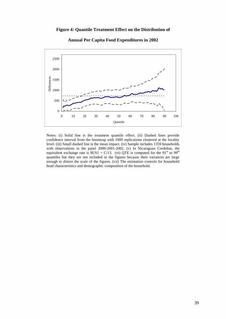
household level varies at different points of the expenditure distribution. Figures 1 through 6

plot the quantiles using post-treatment data. The solid line represents the estimate of the RPS

treatment in a given quantile. The associated 95 percent confidence intervals are obtained

from the bootstrap with 1000 replications clustered at the locality level. These bootstrap

confidence intervals are plotted on the graph with dashed lines. For comparison purposes, the

mean treatment effect is plotted as a small dashed line.17

Overall, RPS treatment group expenditures are greater than control group

expenditures, yielding positive impacts at each quantile of the distribution. For per capita

total expenditures and per capita food expenditures, the difference increases from the lowest

percentile to the highest percentile of the distribution. These findings suggest that households

with lower expenditures tend to receive lower positive impacts from the program. As the

theoretical framework suggests the impacts are greater for households with higher

expenditures who are more likely meeting or almost meeting program requirements prior to

the program. For households with lower expenditures who are more likely not meeting the

requirements and for whom the cost of participation is therefore the highest, program impacts

are still positive but smaller than for households at the upper end of the distribution. These

results are similar to Djebbari and Smith’s (2005) QTE findings for the Mexican’s

PROGRESA. They find that program impacts on wealth and nutrition are greater for

21

households who were at higher levels of wealth and nutrition prior to the program. Similarly,

for the share of food expenditure, the difference decreased from the lowest percentile to the

highest percentile suggesting that the program impacts are higher for households who had

lower levels of food shares prior to the program.18

Figure 1 shows that in 2001 the program impact on per capita total expenditures varies

from about C$707 (US$ 54) to C$3087 (US$ 237). In 2002, the program impact on per capita

total expenditures varies from about C$264 (US$20) to C$1293 (US$99) for the highest

percentile (Figure 2). Many of the impacts are quite large compared to the mean impacts of

C$1184 and C$820 in 2001 and 2002, respectively. These results suggest that households at

the top of the outcome distribution receive more than five times the impact that households

with lower expenditures do.

I test whether a constant treatment effect could lead to a range as large as that

observed for the QTE point estimate as in Bitler et al. (2006). The test is as follows: first,

keep only observations in the control group and assign a uniformly distributed random

number to the ith

household in the bth

bootstrap sample.19

Second, sort the sample of

households using this random number and assign t=1 to households with a random number

higher than 0.5 and in the bth

sample and t=0 to the remaining households in this bootstrap

sample. Third, add the estimated mean treatment effect to households with t=1 to create a

synthetic null treatment group distribution. Finally, use the synthetic null treatment group and

the remaining control group to construct the QTE under the null hypothesis. From the

resulting individual distributions, we can generate a confidence interval for testing the

maximum minus minimum range, which compares the distribution for the range under the

null with the real-data QTE range. This confidence interval is estimated with 1000 bootstrap

replications. The test of constant treatment effects suggests that the null constant treatment

range is [3187.1, 3384.1] and [2987.9, 3198.2] at a confidence level above 95 percent for

22

2001 and 2002, respectively. The QTE range estimated using the data is 2380.3 and 1029.8

for 2001 and 2002. These results show that the mean treatment effect is not sufficient to

characterize RPS’s effects on total per capita expenditures.20

Consistent with the RPS program’s goal, additional expenditures as a result of the

transfers were spent predominantly on food. Results for food expenditures suggest a large

degree of treatment impact heterogeneity. In 2001, the program impact on per capita food

expenditures varies from about C$367 (US$28) to C$3780 (US$290) for the highest

percentile of the distribution (Figure 3). In 2002, the program impact on per capita food

expenditures varies from about C$174 (US$13) to C$1846 (US$142) for the highest

percentile of the distribution (Figure 4). The mean impacts are C$1004 and C$733 for 2002

and 2001, which are far below the impacts at the top of the distribution. The confidence

interval for a null of constant treatment effects is [1963.6, 2104.9] and [1993.8, 2186.4] at a

confidence level of above 95 percent, while the estimated range over all quantiles in the real

data is 3412.2 and 1671.7 for 2001 and 2002, respectively. The positive impact of the

program for households with the highest per capita food expenditures prior to the program is

almost seven times the impact for households with lower food expenditures, which is not

captured by the mean treatment effect estimate.

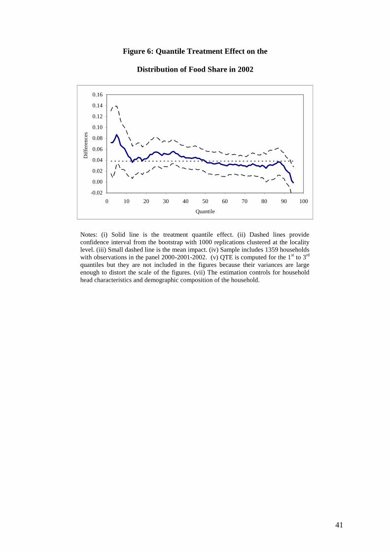
To further explore the impacts of RPS on the distribution of expenditures, Figures 5

and 6 show QTEs for the share of food expenditures in the household budget. In 2001, the

program impact on food share ranges from about 7.79 percentage points to -0.18 percentage

points for the highest percentile. In 2002, the program impact on food share varies from about

8.65 percentage points to -1.42 percentage points for the highest percentile. The mean

impacts are about 4.0 and 3.8 percentage points in 2001 and 2002. The impact is higher for

households who have a lower share of food expenditures prior to the program. Maluccio and

23

Flores (2005) have shown that not only the number of food items purchased increased but

also their nutritional value.

Rank Preservation and Rank Reversal

The main QTE findings show that the impact of the RPS program varied across the

distribution of total and food expenditures. As previously discussed, the impact of the

treatment on the distribution is not the distribution of treatment effects. This interpretation is

valid only under the rank preservation assumption. This section examines whether there is

evidence consistent with rank preservation. As in Bitler et al. (2005), I use the treatment and

control distributions of demographic characteristics to see if there is evidence against rank

preservation or rank reversal in each quartile. For example, if the distribution of observable

characteristics in some range of the expenditures distribution varies significantly between the

treatment and control group, this would be evidence against rank preservation. Note,

however, that rank reversal may have occurred among unobservables even if observable

characteristics do not change.

Tables 5 and 6 present the mean difference by quartile and the p-value for statistical

significance. Each row corresponds to a demographic variable separated by household head

characteristics (gender, education, age, and employment) and household demographic

composition (girls 0-5 years, boys 0-5 years, girls 6-15 years, and boys 6-15 years). The test

is performed for a total of 8 variables and, thus, tables 5 and 6 present 32 tests for each

distribution and year. Panel A classifies people by their position (quartile) in the per capita

total expenditure distribution and Panel B classifies people by their position in the per capita

food expenditure distribution. Table 5 presents the results from the exercise using the 2001

data, whereas Table 6 presents the results using the 2002 data.

24

Of the 128 differences, 18 are statistically significant at the 10 percent level or below

in 2001 and 2002. The individual test suggests that some rank reversal may be present based

on these demographic characteristics. The joint test for the significance of the differences

within a given quantile range, however, fails to reject the null for all ranges of per capita food

expenditure and per capita total expenditure.21

While the individual tests suggest that some

rank reversal may be present along observables, the joint test results show that strict rank

reversal is not rejected.

VI. SUMMARY AND CONCLUSIONS

This paper assesses the importance of heterogeneity in impacts of conditional cash

transfers using a social experiment from a poverty alleviation program in Nicaragua.

Heterogeneity in program impacts is expected to arise because of the design and

implementation of the program. The theoretical model shows that program impacts vary with

observable characteristics, the targeting dimension, and the conditionality of the program.

The first part of the paper analyzes impacts at the subgroup level by estimating the

interaction between the treatment indicator and covariates of interest. The estimates also

show that children living in more impoverished localities experienced larger impacts of the

program on schooling in 2001, but this result is reversed in 2002. The second part of the

paper analyzes quantile treatment effects. The results suggest evidence against the common

effect assumption. The estimates show that the impact of the program is lower for households

who were at a lower level of expenditures prior to the program. That is, the RPS program has

a greater effect on households who would otherwise have had a high per capita total and food

expenditures. Quantile treatment effect estimates show there was considerable heterogeneity

in the impacts of the RPS on the distributions of expenditures, which is missed by looking

only at average treatment effects. As the theoretical framework suggests, the impacts are

25

greater for households with higher expenditures who are more likely to be meeting or almost

meeting program requirements prior to the program. For households with lower expenditures

who are more likely to not be meeting the requirements, and for whom the cost of

participation is the highest, program impacts are still positive but smaller than for households

at the upper end of the distribution. Tests of the null hypothesis of constant treatment effects

reveal that these findings could not have been obtained using mean impact analysis. In

addition, joint tests of rank preservation show that the distributions of observable

characteristics in all ranges of the expenditures distribution do not vary significantly between

the treatment and control group. These results have important implications for the

implementation and evaluation of conditional cash transfers that are spreading rapidly in

developing countries.

26

REFERENCES

Abadie, Alberto, Joshua Angrist, and Guido W. Imbens. 2002. Instrumental Variables

Estimation of Quantile Treatment Effects. Econometrica 70(1):91-117.

Basu, K., Hoang Van, P., 1998. The Economics of Child Labor. American Economic Review,

88: 412-427.

Behrman, Jere R., and Petra Todd. 1999. Randomness in the Experimental Samples of

PROGRESA (Education, Health, and Nutrition Program). Report submitted to

PROGRESA. International Food Policy Research Institute, Washington, D.C.

Behrman, Jere R., Piyali Sengupta, and Petra Todd. 2005. Progressing through PROGRESA:

An Impact Assessment of a School Subsidy Experiment in Rural Mexico. Economic

Development and Cultural Change 54(1): 237–275.

Bitler, Marianne, Jonah Gelbach, and Hilary Hoynes. 2005. Distributional Impacts of the

Self-Sufficiency Project. NBER Working Paper No. 11626. September.

---------------------------------. 2006. What Mean Impact Miss: Distributional Effects of

Welfare Reform Experiments. American Economic Review, 96(4):988-1012.

Black, Dan, Jeffrey Smith, Mark C. Berger, and Brett J. Noel. 2003. Is The Threat of

Reemployment Services More Effective Than The Services Themselves?

Experimental Evidence from the UI System. American Economic Review 93: 1313-

1327.

Deaton, Angus. 1997. The Analysis of Household Surveys: A Microeconometric Approach to

Development Policy. Washington D.C: Johns Hopkins University Press.

Djebbari, Habiba, and Jeffrey Smith. 2005. Heterogeneous Program Impacts in PROGRESA.

Unpublished Manuscript. Department of Economics, Laval University.

------------------------------------------. 2008. Heterogeneous Program Impacts in PROGRESA.

IZA Working Paper No 3362. Forthcoming in Journal of Econometrics.

27

Duflo, Esther, Glennerster, Rachel and Kremer, Michael. 2007. Using Randomization in

Development Economics Research: A Toolkit, in T. Paul Schultz and John Strauss,

eds., Handbook of Development Economics, Volume 4, Amsterdam: North Holland.

Filmer, Deon, and Norbert Schady. 2008. Getting Girls into School: Evidence from a

Scholarship Program in Cambodia. Economic Development and Cultural Change

56(3): 581–617.

Firpo, Sergio. 2007. Efficient Semiparametric Estimation of Quantile Treatment Effects.

Econometrica 75(January): 259-276.

Gertler, Paul. 2004. Do Conditional Cash Transfers Improve Child Health? Evidence from

PROGRESA's Control Randomized Experiment. American Economic Review Papers

and Proceedings 94(2):336-341.

Heckman, James, Jeffrey Smith, and Nancy Clements. 1997. Making the Most Out of

Programme Evaluations and Social Experiments: Accounting for Heterogeneity in

Program Impacts. The Review of Economic Studies 64: 487-535.

Heckman, James, Robert LaLonde, and Jeffrey Smith. 1999. The Economics and

Econometrics of Active Labor Market Programs in Orley Ashenfelter and David Card

(eds.), Handbook of Labor Economics, Volume 3A. Amsterdam: North-Holland, 1865-

2097.

Heckman, James and Jeffrey Smith. 1995. Assessing the Case for Social Experiments.

Journal of Economic Perspectives 9: 85-110.

Koenker, Roger, and Gilbert Basset. 1978. Regression quantiles. Econometrica 46(1): 33-50.

Maluccio, John, and Rafael Flores. 2005. Impact Evaluation of a Conditional Cash Transfer

Program: The Nicaraguan Red de Proteccion Social, FCND Discussion Paper, No.

141, IFPRI, Washington D.C.

28

Maluccio, John, Alexis Murphy, and Fernando Regalia. 2006. Does Supply Matter? Initial

Supply Conditions and the Effectiveness of Conditional Cash Transfers for Schooling

in Nicaragua. Inter-American Development Bank. Manuscript.

Ravallion, Martin. 2005. Evaluating Anti-Poverty Programs in T. Paul Schultz and John

Strauss (eds.), Handbook of Development Economics Volume 4. Forthcoming.

Rawlings, Laura, and Gloria Rubio. 2003. Evaluating the Impact of Conditional Cash

Transfer Programs: Lessons from Latin America. World Bank Policy Research

Working Paper No. 3119. Washington D.C.

Schady, Norbert, and Maria Caridad Araujo. 2006. Cash Transfers, Conditions, School

Enrollment, and Child Work: Evidence from a Randomized Experiment in Ecuador.

World Bank Policy Research Working Paper 3930.

Schultz, T. Paul. 2004. School Subsidies for the Poor: Evaluating the Mexican Progresa

Poverty Program. Journal of Development Economics 74(1): 199-250.

Skoufias, Emmanuel, and Susan Parker. 2001. Conditional Cash Transfers and Their Impact

on Child Work and Schooling: Evidence from the PROGRESA Program in Mexico.

Economia 2: 45–96.

Skoufias, Emmanuel. 2005. PROGRESA and Its Impacts on the Welfare of Rural

Households in Mexico. IFPRI Research Report No. 139. International Food Policy

Research Institute, Washington, D.C.

29

Table 1: Nicaraguan RPS Beneficiary Requirements

Household Type

With no

targeted

children

With

children

aged 0-5

With children

aged 7 -13 who

have not

completed 4th

grade

(A) (B) (C)

Attend bimonthly health education

workshops

Bring children to prescheduled health care

appointments

Monthly ( 0-2 years)

Bimonthly (2-5 years)

Adequate weight gain for children under 5a

Enrollment in grades 1 to 4 of all targeted

children in the household

Regular attendance (85%) of all targeted

children in the household

Promotion at end of school year b

Bono a la Oferta or Teacher transfer

Up-to-date vaccination for all children under

5 years

a This requirement was discontinued in Phase II in 2003

b This condition was not enforced

Source: Maluccio and Flores (2005)

30

Table 2: Descriptive Statistics for Children and Their Households

2000

2001 2002

Household Level

Per Capita Total Consumption 3885.08 3852.74 3880.91

Per Capita Food Consumption 2672.33 2669.20 2634.18

Food Share 0.704 0.688 0.683

Head of Household

Age 44.27 46.05 47.01

Male 0.858 0.858 0.858

Years of Education a 1.652 - -

Children 7-13 years at baseline

Gender 0.521 0.521 0.521

Age 9.847 10.938 11.969

School Attendance 0.766 0.885 0.855

Participation in Labor Activities 0.150 0.109 0.177

Weekly Working Hours 3.51 2.90 5.31

Weekly Working Hours

conditional on employment 23.47 26.49 30.07 a Data available only for 2000

Note: Expenditures levels are in Nicaraguan Cordobas, the equivalent exchange rate is

US$1 = C$13. Sample includes 1359 households with observations in the panel 2000-

2001-2002.

31

Table 3: RPS Summary Statistics: 2000 Baseline

(Standard errors in parentheses)

Treatment

Control Difference

Household Level

Per Capita Total Consumption 4020.90 3738.24 282.66

(203.22) (212.23) (290.34)

Per Capita Food Consumption 2759.87 2577.68 182.193

(129.02) (128.33) (179.81)

Food Share 0.70 0.71 -0.01

(0.01) (0.01) (0.01)

Household Head

Age 44.64 43.86 0.77

(0.85) (0.73) (1.11)

Male 0.87 0.85 0.02

(0.01) (0.01) (0.02)

Years of Education 1.70 1.60 0.10

(0.14) (0.09) (0.16)

N 706 653 1359

Children 7-13 years

Gender 0.53 0.51 0.02

(0.02) (0.02) (0.02)

Age 9.82 9.87 -0.05

(0.07) (0.07) (0.10)

School Attendance 0.77 0.77 0.00

(0.01) (0.01) (0.02)

Participation in Labor Activities 0.14 0.16 -0.02

(0.01) (0.01) (0.02)

Working Hours 3.26 3.78 -0.52

(0.33) (0.37) (0.49)

N 916 829 1745

**Statistically significant at 5% level, *Statistically significant at 10% level (only for differences).

Note: Expenditures levels are in Nicaraguan Cordobas, the equivalent exchange rate is $US1 =

C/13. Robust standard errors, clustered at the locality level. Sample includes 1359 households with

observations in the panel 2000-2001-2002.

32

Table 4: RPS Program Impacts along Observables Characteristics for children 7 to 13 years at baseline


2001 2002

School

Attendance

Participation

in labor

activities

Hours

Worked

(OLS)

Hours

Worked

(Tobit)

School

Attendance

Participation

in labor

activities

Hours

Worked

(OLS)

Hours

Worked

(Tobit)

T*male 0.060** -0.099** -4.034** -8.085 0.063** -0.124** -4.771** -7.330

(0.03) (0.04) (1.07) (9.27) (0.03) (0.04) (1.41) (7.59)

T 0.117** -0.012 -0.383 -12.335 0.110** -0.014 -0.901 -11.778

(0.03) (0.01) (0.31) (8.52) (0.02) (0.02) (0.67) (8.74)

T*age -0.003 -0.019** -0.739** -1.677 0.018 0.000 -0.716* 3.712**

(0.01) (0.01) (0.30) (1.91) (0.01) (0.01) (0.38) (1.75)

T 0.185* 0.145* 5.605* 1.068 -0.068 -0.073 5.165** -65.299**

(0.10) (0.08) (2.81) (23.47) (0.02) (0.11) (3.96) (24.75)

T*Household Head Schooling -0.028** -0.006 -0.203 -1.328 -0.014* -0.007 -0.029 -0.612

(0.01) (0.01) (0.22) (1.90) (0.01) (0.01) (0.26) (1.44)

T 0.195** -0.053** -2.148** -16.812** 0.165** -0.067* -3.352** -16.408**

(0.03) (0.03) (0.80) (5.77) (0.03) (0.04) (1.01) (5.70)

T*Household Head is Male -0.019 0.076* 2.577* 35.752** -0.034 0.005 0.588 -1.361

(0.07) (0.04) (1.39) (13.54) (0.07) (0.06) (2.20) (10.54)

T 0.165** -0.131** -4.759** -51.842** 0.172** -0.082 -3.905* -16.191

(0.06) (0.04) (1.25) (12.70) (0.07) (0.06) (2.26) (12.08)

T*Household Size -0.002 0.011** 0.172 2.377** -0.006 -0.001 0.003 -0.383

(0.01) (0.01) (0.15) (1.19) (0.01) (0.01) (0.27) (1.41)

T 0.164** -0.155** -3.921** -39.437** 0.195** -0.070 -3.410 -14.120

(0.07) (0.05) (1.28) (11.56) (0.05) (0.09) (2.69) (15.04) **Statistically significant at 5% level, *Statistically significant at 10% level. Note: Expenditures levels are in Nicaraguan Cordobas, the equivalent exchange rate is $US1 = C/13.

Robust standard errors, clustered at the locality level. Sample includes 1359 households with observations in the panel 2000-2001-2002.

33

Table 4: RPS Program Impacts along Observables Characteristics for children 7 to 13 years at baseline (continued)


2001 2002

School

Attendance

Participation

in labor

activities

Hours

Worked

(OLS)

Hours

Worked

(Tobit)

School

Attendance

Participation

in labor

activities

Hours

Worked

(OLS)

Hours

Worked

(Tobit)

Quintiles of the Marginality Index

T 0.190** -0.078* -3.117** -24.558** 0.081** -0.072 -1.262 -15.598

(0.08) (0.05) (1.38) (11.17) (0.03) (0.08) (1.25) (11.52)

T*2nd

Quintile -0.039 -0.001 -0.036 2.590 0.112** -0.008 -2.443 -3.149

(0.11) (0.06) (1.88) (15.22) (0.05) (0.09) (2.20) (15.89)

T*3rd

Quintile -0.122 0.100* 3.495** 24.086 -0.018 0.075 0.374 9.348

(0.10) (0.06) (1.70) (17.03) (0.05) (0.09) (2.16) (15.85)

T*4th

Quintile -0.056 0.005 0.689 8.794 0.069 0.009 -2.396 4.925

(0.09) (0.05) (1.81) (12.04) (0.06) (0.11) (2.31) (14.58)

T*5th

Quintile (richest) -0.012 0.017 0.537 4.535 0.107* -0.055 -5.112** -13.667

` (0.11) (0.06) (1.74) (13.35) (0.06) (0.09) (1.92) (14.32)

Quintiles of Household Per Capita Expenditures

T 0.197** -0.032 -2.219* -13.496* 0.200** -0.062 -2.749** -17.976**

(0.06) (0.04) (1.20) (8.38) (0.05) (0.04) (1.36) (7.65)

T*2nd

Quintile -0.001 -0.058 -1.501 -17.453 -0.030 -0.055 -1.228 -4.258

(0.06) (0.05) (1.75) (12.42) (0.06) (0.06) (1.99) (10.06)

T*3rd

Quintile -0.033 0.014 1.547 6.149 -0.103 0.012 -0.048 5.637

(0.06) (0.05) (1.42) (11.30) (0.07) (0.06) (1.83) (10.74)

T*4th

Quintile -0.147** -0.075* -0.748 -14.530 -0.133* 0.010 -0.079 7.082

(0.06) (0.04) (1.42) (10.62) (0.07) (0.06) (1.95) (10.29)

T*5th

Quintile (richest) -0.080 -0.040 -0.562 -3.207 -0.031 -0.048 -1.640 -2.381

(0.06) (0.06) (1.35) (15.80) (0.07) (0.06) (2.02) (10.90)

F-test for the null that all

interactions=0 (p-value)a

4.55

(0.000)

2.48

(0.013)

3.97

(0.000)

23.97b

(0.031)

2.98

(0.004)

2.01

(0.045)

2.28

(0.023)

22.08b

(0.054) **Statistically significant at 5% level, *Statistically significant at 10% level.

a F-test obtained from a equation including all interactions and main effects.

bChi-square test

Note: Expenditures levels are in Nicaraguan Cordobas, the equivalent exchange rate is $US1 = C/13. Robust standard errors, clustered at the locality level. Sample includes 1359

households with observations in the panel 2000-2001-2002.

34

Table 5: Tests of Rank Reversal from Distribution of Observables for Ranges in Expenditure Distribution, 2001

25q 25 50q 50 75q 75q

Mean Diff p-value Mean Diff p-value Mean Diff p-value Mean Diff p-value

Panel A: Per capita Total Expenditure

Distribution Ranges

Household Head is male 0.000 0.016 -0.001 0.609 -0.002 0.497 0.000 0.112

Household Head Years of Education 0.007 0.605 -0.007 0.345 0.004 0.050 0.011 0.058

Household Head is employed 0.000 0.856 0.002 0.441 -0.001 0.649 0.000 0.445

Household Head age -0.012 0.178 0.029 0.816 0.037 0.661 -0.003 0.455

Girls 0-5 years -0.003 0.567 0.001 0.527 0.001 0.972 -0.005 0.617

Girls 5-15 years 0.004 0.515 0.001 0.986 0.002 0.948 -0.009 0.816

Boys 0-5 years 0.005 0.948 0.000 0.513 -0.005 0.002 -0.006 0.178

Boys 5-15 years 0.003 0.820 0.001 0.341 -0.002 0.048 -0.009 0.074

Panel B: Per capita Food Distribution

Ranges

Household Head is male 0.000 0.192 0.001 0.633 -0.004 0.503 0.000 0.150

Household Head Years of Education 0.008 0.583 -0.011 0.593 -0.009 0.140 0.011 0.130

Household Head is employed -0.001 0.463 0.004 0.439 -0.001 0.411 0.000 0.687

Household Head age -0.007 0.108 -0.083 0.471 0.171 0.749 -0.014 0.301

Girls 0-5 years -0.003 0.525 -0.001 0.549 0.003 0.926 -0.004 0.583

Girls 5-15 years 0.007 0.359 -0.002 0.864 -0.002 0.333 -0.009 0.443

Boys 0-5 years 0.004 0.317 0.004 0.523 -0.007 0.002 -0.005 0.062

Boys 5-15 years 0.003 0.497 -0.002 0.222 0.007 0.036 -0.010 0.098

Note: Mean treatment-control differences and p-values for tests of individual differences being significant for each observable characteristic at each quartile. P-values obtained

from the bootstrap with 1000 replications clustered at the locality level. Null distribution derived as in Bitler et. al. (2005).

35

Table 6: Tests of Rank Reversal from Distribution of Observables for Ranges in Expenditure Distribution, 2002

25q 25 50q 50 75q 75q

Mean Diff p-value Mean Diff p-value Mean Diff p-value Mean Diff p-value

Panel A: Per capita Total Expenditure

Distribution Ranges

Household Head is male 0.000 0.695 -0.001 0.371 0.000 0.629 -0.001 0.271

Household Head Years of Education 0.009 0.854 0.011 0.160 0.000 0.749 0.005 0.573

Household Head is employed 0.000 0.617 0.002 0.934 0.000 0.467 -0.001 0.495

Household Head age 0.107 0.391 -0.108 0.774 -0.036 0.383 0.061 0.291

Girls 0-5 years 0.006 0.982 -0.002 0.196 0.000 0.539 -0.007 0.379

Girls 5-15 years -0.003 0.022 0.011 0.112 0.004 0.389 -0.013 0.820

Boys 0-5 years 0.006 0.948 0.000 0.156 -0.001 0.056 -0.007 0.122

Boys 5-15 years 0.005 0.583 -0.002 0.028 0.003 0.944 -0.010 0.110

Panel B: Per capita Food Distribution

Ranges

Household Head is male 0.000 0.365 0.001 0.695 -0.003 0.948 0.000 0.425

Household Head Years of Education 0.014 0.160 0.011 0.904 -0.010 0.902 0.006 0.471

Household Head is employed 0.000 0.665 0.002 0.788 -0.001 0.894 0.000 0.583

Household Head age 0.087 0.423 -0.075 0.170 -0.046 0.866 0.059 0.273

Girls 0-5 years 0.007 0.733 -0.002 0.443 -0.001 0.481 -0.006 0.435

Girls 5-15 years 0.000 0.032 0.012 0.255 0.000 0.084 -0.012 0.890

Boys 0-5 years 0.004 0.471 0.005 0.072 -0.004 0.361 -0.006 0.092

Boys 5-15 years 0.004 0.950 0.002 0.008 0.004 0.549 -0.011 0.248

Note: Mean treatment-control differences and p-values for tests of individual differences being significant for each observable characteristic. P-values obtained from the

bootstrap with 1000 replications clustered at the locality level. Null distribution derived as in Bitler et. al. (2005).

36

Figure 1: Quantile Treatment Effect on the Distribution of

Annual Per Capita Total Expenditures in 2001

-100

400

900

1400

1900

2400

0 10 20 30 40 50 60 70 80 90 100

Quantile

Dif

fere

nce

s

Notes: (i) Solid line is the treatment quantile effect. (ii) Dashed lines provide

confidence interval from the bootstrap with 1000 replications clustered at the locality

level. (iii) Small dashed line is the mean impact. (iv) Sample includes 1359 households

with observations in the panel 2000-2001-2002. (v) In Nicaraguan Cordobas, the

equivalent exchange rate is $US1 = C/13. (vi) QTE is computed for the 91st to 99

th

quantiles but they are not included in the figures because their variances are large

enough to distort the scale of the figures. (vii) The estimation controls for household

head characteristics and demographic composition of the household.

37



-100

400

900

1400

1900

2400

0 10 20 30 40 50 60 70 80 90 100

Quantile

Dif

fere

nce

s






th




38


Annual Per Capita Food Expenditures in 2001

0

500

1000

1500

2000

2500

0 10 20 30 40 50 60 70 80 90 100

Quantile

Dif

fere

nce

s






th




39



0

500

1000

1500

2000

2500

0 10 20 30 40 50 60 70 80 90 100

Quantile

Dif

fere

nce

s






th




40

Figure 5: Quantile Treatment Effect on the

Distribution of Food Share in 2001

-0.02

0.00

0.02

0.04

0.06

0.08

0.10

0.12

0.14

0.16

0 10 20 30 40 50 60 70 80 90 100

Quantile

Dif

fere

nce

s




with observations in the panel 2000-2001-2002. (v) QTE is computed for the 1st to 3

rd




41

Figure 6: Quantile Treatment Effect on the

Distribution of Food Share in 2002

-0.02

0.00

0.02

0.04

0.06

0.08

0.10

0.12

0.14

0.16

0 10 20 30 40 50 60 70 80 90 100

Quantile

Dif

fere

nce

s




with observations in the panel 2000-2001-2002. (v) QTE is computed for the 1st to 3

rd




42

Appendix Figure A.1: Quantile Treatment Effect on the Distribution of


-1200

-700

-200

300

800

1300

1800

0 10 20 30 40 50 60 70 80 90 100

Quantile

Dif

fere

nces






th


enough to distort the scale of the figures

43

Figure A.2: Quantile Treatment Effect on the Distribution of


-1200

-700

-200

300

800

1300

1800

0 10 20 30 40 50 60 70 80 90 100

Quantile

Dif

fere

nces






th


enough to distort the scale of the figures.

44

* I am grateful for helpful comments and suggestions from Dan Black, Jeff Kubik, Jose

Galdo, Hugo Ñopo, the editor, and two anonymous referees. I also thank comments and

suggestions received at LACEA in Bogota and the Third IZA/World Bank Conference on

Employment and Development in Rabat. I am grateful to IFPRI for permission to use the

data. Some of the revision on this article was completed while the author was a postdoctoral

fellow in the Economics Department at McMaster University, Canada. Any errors or

omissions are my own responsibility. Correspondence to: Ana C. Dammert, Department of

Economics and NPSIA, Carleton University, Loeb B846, 1125 Colonel by Drive, Ottawa

K1S5B6, Canada.

1 The RPS program did not identify poor households within targeted localities as in

PROGRESA. See Maluccio and Flores (2005) for an assessment of the targeting procedure.

2 Children are required to enroll and attend classes at least 85 percent of the time, i.e., no

more than 5 absences every 2 months without valid excuse.

3 This design seems to embody a perverse incentive for students to keep repeating the 4th

grade so that families can continue to receive the subsidy. In order to eliminate this problem,

the program design included a number of causes for which the household may be expelled

from the program, among them, if the beneficiary child failed to be promoted to the next

grade. This condition, however, was deemed unfair and never enforced. Thanks to the referee

for pointing this out.

4 The lump sum transfer for school supplies and uniforms varies with the number of eligible

children while the school attendance transfer is a lump sum per household, regardless of the

number of children.

5 The evaluation was designed to last for one year but because of delays in funding the

implementation of the program was postponed in control localities until 2003.

45

6 In panel data, both non-response and attrition are potential concerns for the empirical

analysis. In 2001 and 2002, about 92 percent and 88 percent of the targeted households were

re-interviewed, respectively. The principal reasons for failure to interview targeted sample

households were that household members were temporarily absent or that the dwelling

appeared to be uninhabited. Maluccio and Flores (2005) examine the correlates of the

observed attrition and conclude that attrition is not a major concern for estimating program

effects and emphasize that using only the balanced panel is likely to slightly underestimate

the effects.

7 For PROGRESA, Behrman and Todd (1999) found that treatment and control groups had

similar mean outcomes at the locality level before the program; however, they find small

differences at the household and individual level. Thanks to the referee for pointing this out.

8 Maluccio and Flores (2005) analyze 15 indicators and find small differences only in

household size and number of children younger than 5 years old.

9 In the RPS data, approximately 20 percent of the beneficiary households had no targeted

children, 25 percent only children under age 5, 20 percent only children ages 7–13, and the

remaining 35 percent both under 5 year-olds and 7–13 year-olds.

10 See Duflo, Glennerster, and Kremer (2007) for a methodological discussion of

randomization of experiments in developing countries.

11 See Koenker and Basset (1978).

12 Including covariates in the estimation of quantile treatment effects changes somewhat the

nature of the treatment effect being estimated and the assumption that underlies it (see

Djebbari and Smith 2008). Thanks to the referee for pointing this out.

13 Unreported regressions show that the QTE estimates, without controlling for covariates, are

in the 95 percent range of the QTE estimates controlling for covariates. With non-

46

experimental data, the estimation can adjust for differences in baseline observable

characteristics by using propensity score weighting as in Bitler et al. (2006) and Firpo (2007).

14 Labor laws in Nicaragua establish age fourteen as the basic minimum age for work.

Children between the ages of 14 and 17 can work a maximum of six hours per day but not at

night. The employment of youth is prohibited in places that endanger their health and safety

such as mines, garbage dumps, and night entertainment venues (i.e. nightclubs, bars, etc.).

Government enforcement, however, is far from strict.

15 See Maluccio and Flores (2005) for more detailed information on the constructed variables.

16 Quintiles of the marginality index are defined such as the lowest quintile includes people

with the highest marginality index (poorest), whereas the highest quintile includes those with

the lowest marginality index (richest).

17 The bootstrap samples are drawn in a manner that mimics the stratified cluster sample

design of the RPS survey by first drawing localities for each bootstrap sample and then

sampling within the selected localities for each bootstrap sample. QTEs are calculated for

each bootstrap sample and the process is repeated 1,000 times. The standard deviation of a

QTE over the bootstrap replications is an estimator of the standard error.

18 Figures A.1 and A.2 show the QTE estimates for the year before random assignment. The

structure of the figures is identical to tat of Figures 1 to 6before; they show the mean effect,

the QTEs, and the bootstrap 95 percent confidence interval of the QTEs. The effects are

statistically not significantly different from zero for all quantiles.

19 Note that each bootstrap sample has the same size as the control group and sampling is

made with replacement from the observations from the control group only.

20 Using the bootstrap, we can compare the mean range from the null of constant treatment

effect with the mean range from the real data. One-sided tests show that we can reject the null

of equality at the 5 percent level for all variables and years, separately.

47

21

See Bitler et al. (2005) for a detailed explanation of the joint test for the significance of the

demographic variables.

Documents

HETEROGENEOUS IMPACTS OF CONDITIONAL CASH TRANSFERS: EVIDENCE FROM …ftp.iza.org/dp3653.pdf · 2008-08-21 · IZA Discussion Paper No. 3653 August 2008 ABSTRACT Heterogeneous Impacts