Embed Size (px)
Citation preview
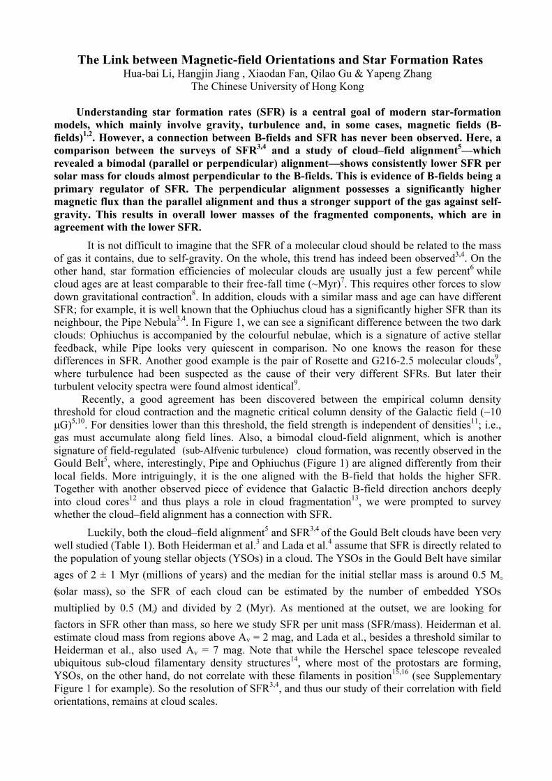
The Link between Magnetic-field Orientations and Star Formation Rates Hua-bai Li, Hangjin Jiang , Xiaodan Fan, Qilao Gu & Yapeng Zhang
The Chinese University of Hong Kong Understanding star formation rates (SFR) is a central goal of modern star-formation models, which mainly involve gravity, turbulence and, in some cases, magnetic fields (B-fields)1,2. However, a connection between B-fields and SFR has never been observed. Here, a comparison between the surveys of SFR3,4 and a study of cloud–field alignment5—which revealed a bimodal (parallel or perpendicular) alignment—shows consistently lower SFR per solar mass for clouds almost perpendicular to the B-fields. This is evidence of B-fields being a primary regulator of SFR. The perpendicular alignment possesses a significantly higher magnetic flux than the parallel alignment and thus a stronger support of the gas against self-gravity. This results in overall lower masses of the fragmented components, which are in agreement with the lower SFR.
It is not difficult to imagine that the SFR of a molecular cloud should be related to the mass of gas it contains, due to self-gravity. On the whole, this trend has indeed been observed3,4. On the other hand, star formation efficiencies of molecular clouds are usually just a few percent6 while cloud ages are at least comparable to their free-fall time (~Myr)7. This requires other forces to slow down gravitational contraction8. In addition, clouds with a similar mass and age can have different SFR; for example, it is well known that the Ophiuchus cloud has a significantly higher SFR than its neighbour, the Pipe Nebula3,4. In Figure 1, we can see a significant difference between the two dark clouds: Ophiuchus is accompanied by the colourful nebulae, which is a signature of active stellar feedback, while Pipe looks very quiescent in comparison. No one knows the reason for these differences in SFR. Another good example is the pair of Rosette and G216-2.5 molecular clouds9, where turbulence had been suspected as the cause of their very different SFRs. But later their turbulent velocity spectra were found almost identical9. Recently, a good agreement has been discovered between the empirical column density threshold for cloud contraction and the magnetic critical column density of the Galactic field (~10 µG)5,10. For densities lower than this threshold, the field strength is independent of densities11; i.e., gas must accumulate along field lines. Also, a bimodal cloud-field alignment, which is another signature of field-regulated (sub-Alfvenic turbulence) cloud formation, was recently observed in the Gould Belt5, where, interestingly, Pipe and Ophiuchus (Figure 1) are aligned differently from their local fields. More intriguingly, it is the one aligned with the B-field that holds the higher SFR. Together with another observed piece of evidence that Galactic B-field direction anchors deeply into cloud cores12 and thus plays a role in cloud fragmentation13, we were prompted to survey whether the cloud–field alignment has a connection with SFR.
Luckily, both the cloud–field alignment5 and SFR3,4 of the Gould Belt clouds have been very well studied (Table 1). Both Heiderman et al.3 and Lada et al.4 assume that SFR is directly related to the population of young stellar objects (YSOs) in a cloud. The YSOs in the Gould Belt have similar ages of 2 ± 1 Myr (millions of years) and the median for the initial stellar mass is around 0.5 M� (solar mass), so the SFR of each cloud can be estimated by the number of embedded YSOs multiplied by 0.5 (M�) and divided by 2 (Myr). As mentioned at the outset, we are looking for factors in SFR other than mass, so here we study SFR per unit mass (SFR/mass). Heiderman et al. estimate cloud mass from regions above Av = 2 mag, and Lada et al., besides a threshold similar to Heiderman et al., also used Av = 7 mag. Note that while the Herschel space telescope revealed ubiquitous sub-cloud filamentary density structures14, where most of the protostars are forming, YSOs, on the other hand, do not correlate with these filaments in position15,16 (see Supplementary Figure 1 for example). So the resolution of SFR3,4, and thus our study of their correlation with field orientations, remains at cloud scales.
(sub-Alfvenic turbulence)
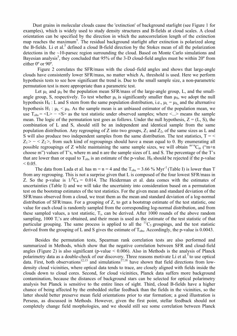
Dust grains in molecular clouds cause the 'extinction' of background starlight (see Figure 1 for examples), which is widely used to study density structures and B-fields at cloud scales. A cloud orientation can be specified by the direction in which the autocorrelation length of the extinction map reaches the maximum5. The residual background starlight after extinction is polarized along the B-fields. Li et al.5 defined a cloud B-field direction by the Stokes mean of all the polarization detections in the ~10-parsec region surrounding the cloud. Based on Monte Carlo simulations and Bayesian analysis5, they concluded that 95% of the 3-D cloud-field angles must be within 20º from either 0º or 90º. Figure 2 correlates the SFR/mass with the cloud–field angles and shows that large-angle clouds have consistently lower SFR/mass, no matter which Av threshold is used. Here we perform hypothesis tests to see how significant the trend is. Due to the small sample size, a non-parametric permutation test is more appropriate than a parametric test. Let µL and µS be the population mean SFR/mass of the large-angle group, L, and the small-angle group, S, respectively. To test whether µL is significantly smaller than µS, we adopt the null hypothesis H0 : L and S stem from the same population distribution, i.e., µL = µS, and the alternative hypothesis H1 : µL < µS. As the sample mean is an unbiased estimator of the population mean, we use Tobs = <L> − <S> as the test statistic under observed samples; where <...> means the sample mean. The logic of the permutation test goes as follows. Under the null hypothesis, Z = (L, S), the combination of L and S, should still be an independent and identical sample from the same population distribution. Any regrouping of Z into two groups, Z1 and Z2, of the same sizes as L and S will also produce two independent samples from the same distribution. The test statistics, T = < Z1 > − < Z2 >, from such kind of regroupings should have a mean equal to 0. By enumerating all possible regroupings of Z while maintaining the same sample sizes, we will obtain m+nCm (“m+n choose m”) values of T’s, where m and n are the sample sizes of L and S. The percentage of the T’s that are lower than or equal to Tobs is an estimate of the p-value. H0 should be rejected if the p-value < 0.05. The data from Lada et al. has m = n = 4 and the Tobs = 3.66 % Myr-1 (Table I) is lower than T from any regrouping. This is not a surprise given that L is composed of the four lowest SFR/mass in Z. So the p-value is 1/8C4 = 0.014. The Heiderman et al. data comes with the estimates of uncertainties (Table I) and we will take the uncertainty into consideration based on a permutation test on the bootstrap estimates of the test statistics. For the given mean and standard deviation of the SFR/mass observed from a cloud, we treat them as the mean and standard deviation of a log-normal distribution of SFR/mass. For a grouping of Z, to get a bootstrap estimate of the test statistic, one value for each cloud is randomly sampled from the corresponding log-normal distribution, and from these sampled values, a test statistic, Ti, can be derived. After 1000 rounds of the above random sampling, 1000 Ti’s are obtained, and their mean is used as the estimate of the test statistic of that particular grouping. The same process is applied to all the 11C5 groupings, and the test statistic derived from the grouping of L and S gives the estimate of Tobs. Accordingly, the p-value is 0.0043.
Besides the permutation tests, Spearman rank correlation tests are also performed and summarized in Methods, which show that the negative correlation between SFR and cloud-field angles (Figure 2) is also significant (p-value < 0.006). Also in Methods is the analysis of Planck polarimetry data as a double-check of our discovery. Three reasons motivate Li et al.5 to use optical data. First, both observations12,13 and simulations17,18 have shown that field directions from low-density cloud vicinities, where optical data tends to trace, are closely aligned with fields inside the clouds down to cloud cores. Second, for cloud vicinities, Planck data suffers more background contamination, because the distances of background stars can be selected for optical polarimetry analysis but Planck is sensitive to the entire lines of sight. Third, cloud B-fields have a higher chance of being affected by the embedded stellar feedback than the fields in the vicinities, so the latter should better preserve mean field orientations prior to star formation; a good illustration is Perseus, as discussed in Methods. However, given the first point, stellar feedback should not completely change field morphologies, and we should still see some correlation between Planck
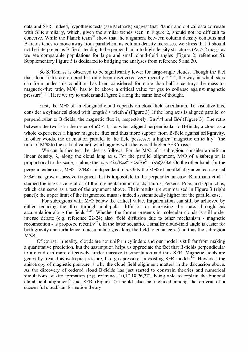
data and SFR. Indeed, hypothesis tests (see Methods) suggest that Planck and optical data correlate with SFR similarly, which, given the similar trends seen in Figure 2, should not be difficult to conceive. While the Planck team30 show that the alignment between column density contours and B-fields tends to move away from parallelism as column density increases, we stress that it should not be interpreted as B-fields tending to be perpendicular to high-density structures (AV > 2 mag), as we see comparable populations for large and small cloud-field angles (Figure 2; reference 5). Supplementary Figure 5 is dedicated to bridging the analyses from reference 5 and 30.
So SFR/mass is observed to be significantly lower for large-angle clouds. Though the fact that cloud fields are ordered has only been discovered very recently10,12,13, the way in which stars can form under this condition has been considered for more than half a century: the mass-to-magnetic-flux ratio, M/Φ, has to be above a critical value for gas to collapse against magnetic pressure19,20. Here we try to understand Figure 2 along the same line of thought.
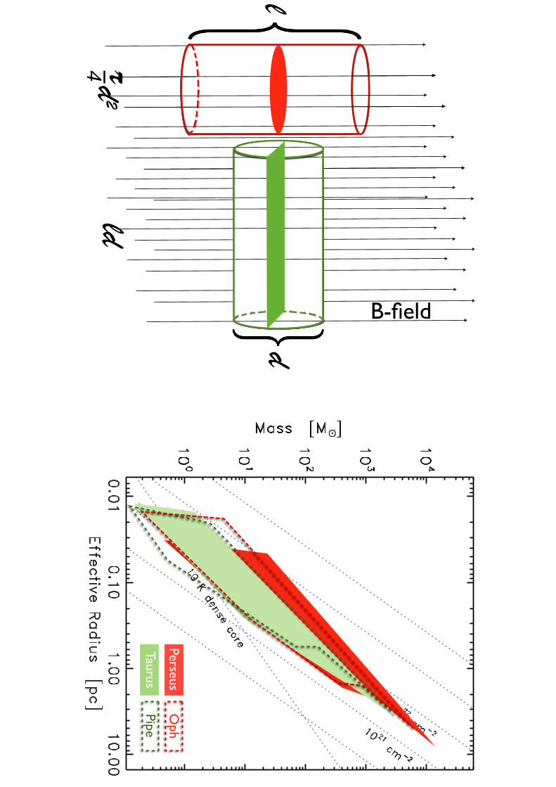
First, the M/Φ of an elongated cloud depends on cloud-field orientation. To visualize this, consider a cylindrical cloud with length l > width d (Figure 3). If the long axis is aligned parallel or perpendicular to B-fields, the magnetic flux is, respectively, Bπd2/4 and Bld (Figure 3). The ratio between the two is in the order of d/l < 1, i.e. when aligned perpendicular to B-fields, a cloud as a whole experiences a higher magnetic flux and thus more support from B-field against self-gravity. In other words, the orientation parallel to the field possesses a higher “magnetic criticality” (the ratio of M/Φ to the critical value), which agrees with the overall higher SFR/mass. We can further test the idea as follows. For the M/Φ of a subregion, consider a uniform linear density, λ, along the cloud long axis. For the parallel alignment, M/Φ of a subregion is proportional to the scale, s, along the axis: 4λs/Bπd2 ≃ λs/Bd2 = (s/d)λ/Bd. On the other hand, for the perpendicular case, M/Φ = λ/Bd is independent of s. Only the M/Φ of parallel alignment can exceed λ/Bd and grow a massive fragment that is impossible in the perpendicular case. Kaufmann et al.21 studied the mass-size relation of the fragmentation in clouds Taurus, Perseus, Pipe, and Ophiuchus, which can serve as a test of the argument above. Their results are summarised in Figure 3 (right panel): the upper limit of the fragmented mass is indeed systematically higher for the parallel case. For subregions with M/Φ below the critical value, fragmentation can still be achieved by either reducing the flux through ambipolar diffusion or increasing the mass through gas accumulation along the fields19,20. Whether the former presents in molecular clouds is still under intense debate (e.g. reference 22-24; also, field diffusion due to other mechanism - magnetic reconnection - is proposed recently25). In the latter scenario, a smaller cloud-field angle is easier for both gravity and turbulence to accumulate gas along the field to enhance λ (and thus the subregion M/Φ). Of course, in reality, clouds are not uniform cylinders and our model is still far from making a quantitative prediction, but the assumption helps us appreciate the fact that B-fields perpendicular to a cloud can more effectively hinder massive fragmentation and thus SFR. Magnetic fields are generally treated as isotropic pressure, like gas pressure, in existing SFR models1,2. However, the anisotropy of magnetic pressure is why the cloud-field alignment matters in the discussion above. As the discovery of ordered cloud B-fields has just started to constrain theories and numerical simulations of star formation (e.g. reference 10,17,18,26,27), being able to explain the bimodal cloud-field alignment5 and SFR (Figure 2) should also be included among the criteria of a successful cloud/star-formation theory.
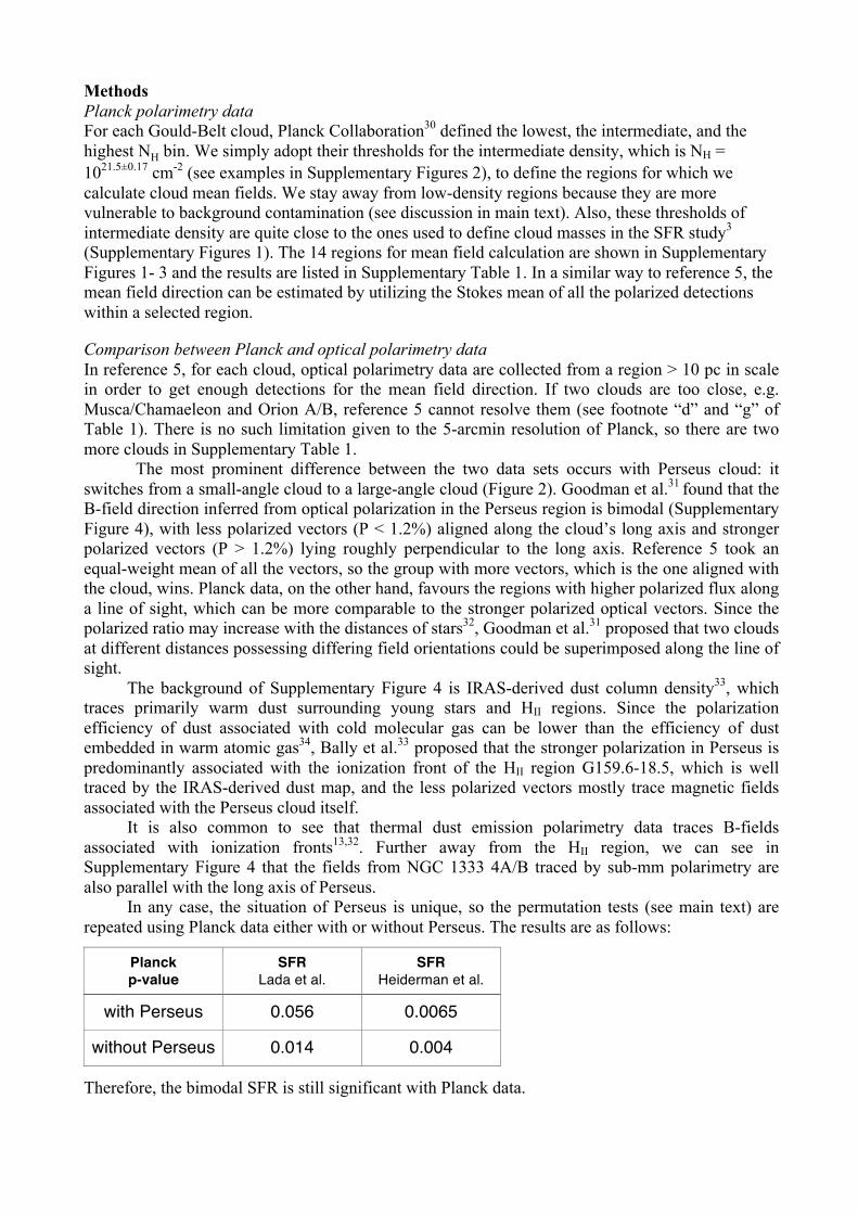
Methods Planck polarimetry data For each Gould-Belt cloud, Planck Collaboration30 defined the lowest, the intermediate, and the highest NH bin. We simply adopt their thresholds for the intermediate density, which is NH = 1021.5±0.17 cm-2 (see examples in Supplementary Figures 2), to define the regions for which we calculate cloud mean fields. We stay away from low-density regions because they are more vulnerable to background contamination (see discussion in main text). Also, these thresholds of intermediate density are quite close to the ones used to define cloud masses in the SFR study3 (Supplementary Figures 1). The 14 regions for mean field calculation are shown in Supplementary Figures 1- 3 and the results are listed in Supplementary Table 1. In a similar way to reference 5, the mean field direction can be estimated by utilizing the Stokes mean of all the polarized detections within a selected region.
Comparison between Planck and optical polarimetry data In reference 5, for each cloud, optical polarimetry data are collected from a region > 10 pc in scale in order to get enough detections for the mean field direction. If two clouds are too close, e.g. Musca/Chamaeleon and Orion A/B, reference 5 cannot resolve them (see footnote “d” and “g” of Table 1). There is no such limitation given to the 5-arcmin resolution of Planck, so there are two more clouds in Supplementary Table 1. The most prominent difference between the two data sets occurs with Perseus cloud: it switches from a small-angle cloud to a large-angle cloud (Figure 2). Goodman et al.31 found that the B-field direction inferred from optical polarization in the Perseus region is bimodal (Supplementary Figure 4), with less polarized vectors (P < 1.2%) aligned along the cloud’s long axis and stronger polarized vectors (P > 1.2%) lying roughly perpendicular to the long axis. Reference 5 took an equal-weight mean of all the vectors, so the group with more vectors, which is the one aligned with the cloud, wins. Planck data, on the other hand, favours the regions with higher polarized flux along a line of sight, which can be more comparable to the stronger polarized optical vectors. Since the polarized ratio may increase with the distances of stars32, Goodman et al.31 proposed that two clouds at different distances possessing differing field orientations could be superimposed along the line of sight. The background of Supplementary Figure 4 is IRAS-derived dust column density33, which traces primarily warm dust surrounding young stars and HII regions. Since the polarization efficiency of dust associated with cold molecular gas can be lower than the efficiency of dust embedded in warm atomic gas34, Bally et al.33 proposed that the stronger polarization in Perseus is predominantly associated with the ionization front of the HII region G159.6-18.5, which is well traced by the IRAS-derived dust map, and the less polarized vectors mostly trace magnetic fields associated with the Perseus cloud itself. It is also common to see that thermal dust emission polarimetry data traces B-fields associated with ionization fronts13,32. Further away from the HII region, we can see in Supplementary Figure 4 that the fields from NGC 1333 4A/B traced by sub-mm polarimetry are also parallel with the long axis of Perseus. In any case, the situation of Perseus is unique, so the permutation tests (see main text) are repeated using Planck data either with or without Perseus. The results are as follows:
Planck p-value
SFR Lada et al.
SFR Heiderman et al.
with Perseus 0.056 0.0065
without Perseus 0.014 0.004
Therefore, the bimodal SFR is still significant with Planck data.

Spearman rank correlation test While reference 5 has concluded a 3-D bimodal cloud-field alignment, and we adopted this point of view to show that SFR/mass can also be divided into two groups, it is difficult to distinguish “two clusters” from “one decreasing trend” for the plots in Figure 2. The mass-to-flux model we proposed to explain Figure 2 is consistent with both possibilities. So here we study how significant the decreasing trend is. We use Spearman rank correlation (SRC) test, which is based on the Pearson Correlation Coefficient between the ranks of two marginal observations. Since the SRC test is based purely on ranks instead of the original quantities, it is insensitive to outliers. For our cases, SRC(rankSFR, rankcf) are between the ranks of SFR, rankSFR, and the ranks of cloud-field angles, rankcf; they are as follows:
SRC (p-value)
SFR Lada et al.
SFR Heiderman et al.
Optical -0.83 (0.006)
-0.75 (≈ 0)
Planck -0.61 (0.043)
-0.81 (≈ 0)
SRC ranges within ± 1; the more positive/negative a SRC is, the more positively/negatively correlated are the ranks. SRC ≈ 0 means no correlation. Therefore, a negative correlation between SFR and cloud-field angles, i.e. a decreasing trend in Figure 2, is clearly based on the observed SRCs (SRCobs) in the above table. In a similar way to the permutation tests for the bimodality, we perform a permutation test for the decreasing trend. For the SFR from Lada et al.4, we randomly permute rankSFR to generate rankSFR_rand_i, for i = 1, 2, ..., k, where k is the total number of permutations used for p-value estimation. We adopt the null hypothesis H0 : SRC(rankSFR, rankcf) = 0, and the alternative hypothesis H1 : SRC(rankSFR, rankcf) < 0. The p-value is thus estimated by the relative frequency to obtain SRC(rankSFR_rand_i, rankcf) < SRCobs. The p-values in the table above are estimated with k = 1000. For the SFR and their uncertainties from Heiderman et al.3, again, we treat them as the means and standard deviations of log-normal distributions. To obtain a bootstrap sample, we sample one value for each cloud from their corresponding log-normal distribution. In a similar way to the Lada et al. data, a p-value can be estimated by permutation for this particular bootstrap sample. By repeating this sampling N times, we obtained N resampling p-values (p1, p2, ..., pN), which resulted from N independent and identically distributed samples. Let
data from Heiderman et al., we treat them as the mean and standard deviation of a log-normal distribution,which denotes what we may observe from this cloud. To get a bootstrap sample, we sample one value for eachcloud from their corresponding log-normal distribution. The classical exact permutation test is applied on thisparametric bootstrap sample to get a p-value. By repeating this resampling-test procedure for N times, wehave N resampling p-values (p1, · · · , pN ), which are resulted from N independent and identically distributed
samples. Let Sobs
= �2P
N
t=1 log(pt). Theoretically, under the null hypothesis H0 is true, S follows a chi-squaredistribution with degree of freedom 2N . If the alternative hypothesis H1 is true, these resampling p-values shallbe small and S shall be large. Thus the final p-value is equal to Pr(�2
2N > Sobs
), where �22N is a chi-square
random variable with degree of freedom 2N . The pseudo-code of this algorithm is given in Algorithm 1. ForN = 1000, the resulting p-value is nearly zero no matter which case we use to treat the cloud Chamaeleon.
Exact permutation test on bootstrap estimates of the test statistic. In this algorithm, we firstenumerate all possible regroupings of the clouds (i.e., simultaneously regroup the mean and standard deviationdata). For each regrouping, we sample a value from the corresponding log-normal distribution of each cloud,thus producing a parametric bootstrap sample for this regrouping and resulting in a test statistic T
b
. Theresampling is repeated for N times for each regrouping. We take the mean test statistic T
B
= 1N
PN
b=1 Tb
as thebootstrap estimate of the test statistic from this regrouping. The K mean test statistic values from all possibleregroupings are compared with the mean test statistic TB
obs
calculated from the original grouping to estimatethe final p-value. The pseudo-code of this algorithm is given in Algorithm 2. Taking N = 1000, this algorithmgives p-value= 0.00476 < 0.05 for the case (a) and (b), and p-value= 0.0043 < 0.05 for the case (c).
Algorithm 2: Exact permutation test on bootstrap estimates of the test statistic
1 Input:2 Z = (X,Y ), where X and Y are observations from the large- and small-angle group respectivley;3 s = (s
X
, sY
), where sX
and sY
are the corresponding observation uncertainty (standard deviation);4 N : bootstrap resample size;5 Output: p-value of the test;6 Initials: n=length(X); m=length(Y); K = Cn
n+m
;
7 Step 1:Obtain the empirical distribution of test statistic under null hypothesis8 for t in 1:K do9 get the t-th regrouping (X⇤, Y ⇤) and (s⇤
X
, s⇤Y
);10 for b in 1:N do11 for i in 1:n do12 sample X
B
[i] from a log-normal distribution with mean=X⇤[i] and standard deviation=s⇤X
[i]);13 end14 for i in 1:m do15 sample Y
B
[i] from a log-normal distribution with mean=Y ⇤[i] and standard deviation=s⇤Y
[i]);16 end17 T [b] = X
B
� YB
, i.e., the mean di↵rence
18 end
19 TB
[t] = 1N
PN
b=1 T [b]
20 end21 Step 2: Obtain the test statistic from the original observed data22 for b in 1:N do23 for i in 1:n do24 sample X
B
[i] from a log-normal distribution with mean=X[i] and standard deviation=sX
[i]);25 end26 for i in 1:m do27 sample Y
B
[i] from a log-normal distribution with mean=Y [i] and standard deviation=sY
[i]);28 end29 T [b] = X
B
� YB
, i.e., the mean di↵rence
30 end
31 TB
obs
= 1N
PN
b=1 T [b]
32 p-value= 1K
PK
t=1(TB
[t] TB
obs
)
In conclusion, both algorithms showed that the large-angle group has a significantly smaller mean SFR/massvalue than the small-angle group.
2
, Sobs is known to follow a chi-square distribution with degree of freedom 2N if H0 is true. Thus the p-value is estimated by the right-tail probability P(!2
2N > Sobs). The decreasing trends are highly significant based on the p-values reported in the above table, where N=1000. Data availability The observational data that support the plots within this paper and other findings of this study can be found from references 3-5 and 30. The Planck 353 GHz data can be downloaded from http://pla.esac.esa.int/pla/#maps.
References 1. Padoan, P. et al in Protostars and Planets VI (eds Beuther, H., Klessen, R., Dullemond,
C. & Henning, Th.) 77-100 (Univ. Arizona Press, 2014) 2. Federrath, C. & Klessen, R. The star formation rate of turbulent magnetized clouds: comparing
theory, simulations, and observations. Astrophys. J. 761, 156 (2012) 3. Heiderman, A., Evans, N. J., II, Allen, L., Huard, T. & Heyer, M. The star formation rate and gas
surface density relation in the Milky Way: implications for extragalactic studies. Astrophys. J. 723, 1019-1037 (2010)
4. Lada, C., Lombardi, M. & Alves, J. On the star formation rates in molecular clouds. Astrophys. J. 724, 687-693 (2010)
5. Li, H.-b., Fang, M., Henning, T. & Kainulainen, J. The link between magnetic fields and filamentary clouds: bimodal cloud orientations in the Gould Belt. Mon. Not. R. Astron. Soc. 436, 3707-3719 (2013)
6. Krumholz, M., Dekel, A. & McKee, C. A universal, local star formation law in galactic clouds, nearby galaxies, high-redshift disks, and starbursts. Astrophys. J. 745, 69 (2012)
7. Lada, C. Star formation in the galaxy: an observational overview. Prog. Theor. Phys. Supplement. 158, 1-23 (2005)
8. Federrath C. Inefficient star formation through turbulence, magnetic fields and feedback. Mon. Not. R. Astron. Soc. 450, 4035-4042 (2015)
9. Heyer, M., Williams, J. & Brunt, C. Turbulent gas flows in the Rosette and G216-2.5 molecular clouds: assessing turbulent fragmentation descriptions of star formation. Astrophys. J. 643, 956-964 (2006)
10. Li, H.-b. et al. in Protostars and Planets VI (eds Beuther, H., Klessen, R., Dullemond, C. & Henning, Th.) 101-123 (Univ. Arizona Press, 2014) 11. Crutcher, R., Wandelt, B., Heiles, C., Falgarone, E. & Troland, T. Magnetic fields in interstellar clouds from Zeeman observations: inference of total field strengths by Bayesian analysis. Astrophys. J. 725, 466-479 (2010) 12. Li, H.-b., Dowell, C. D., Goodman, A., Hildebrand, R. & Novak, G. Anchoring magnetic field in trbulent molecular clouds. Astrophys. J. 704, 891-897 (2009) 13. Li, H.-b. et al. Self-similar fragmentation regulated by magnetic fields in a region forming massive stars. Nature 520, 518-521 (2015) 14. Arzoumanian, D. et al. Characterizing interstellar filaments with Herschel in IC 5146. Astron. Astrophys. 529, L6 (2011) 15. Gutermuth, R. et al. A Spitzer Survey of young stellar clusters within one kiloparsec of the Sun: cluster core extraction and basic structural analysis. Astrophys. J. 184, 18-83 (2009) 16. Stutz, A. & Gould, A. Slingshot mechanism in Orion: kinematic evidence for ejection of protostars by fliaments. Astron. Astrophys. 590, A2 (2016) 17. Otto, F., Ji, W. & Li, H.-b. Velocity anisotropy in self-gravitating molecular clouds. I. simulation Astrophys. J. 836, 95 (2017) 18. Li, P. S., McKee, C. F. & Klein, R. I. Magnetized interstellar molecular clouds – I. comparison between simulations and Zeeman observations. Mon. Not. R. Astron. Soc. 452, 2500-2527 (2015) 19. Mestel, L. Quart. J. R. Problems of Star Formation - II. Quart. J. Roy. Astron. Soc. 6, 265 (1965) 20. Strittmatter, P. A. Gravitational collapse in the presence of a magnetic field. Mon. Not. R. Astr. Soc. 132, 359 (1966) 21. Kauffmann, J., Pillai, T., Shetty, R., Myers, P., Goodman, A. The mass-size relation from clouds to cores. II. solar neighborhood clouds. Astrophys. J. 716, 433-445 (2010) 22. Crutcher, R., Hakobian, N. & Troland, T. Testing magnetic star formation theory. Astrophys. J. 692, 844-855 (2009) 23. Mouschovias, T. & Tassis, K. Testing molecular-cloud fragmentation theories: self-consistent analysis of OH Zeeman observations. Mon. Not. R. Astron. Soc. 400, L15-L19 (2009) 24. Bertram, E., Federrath, C., Banerjee, R. & Klessen, R. S. Statistical analysis of the mass-to-flux ratio in turbulent cores: effects of magnetic field reversals and dynamo amplification. Mon. Not.

R. Astron. Soc. 420, 3163-3173 (2012) 25. Lazarian, A., Esquivel, A. & Crutcher, R. Magnetization of cloud cores and envelopes and other observational consequences of reconnection diffusion. Astrophys. J. 757, 154 (2012) 26. Crutcher, R. Magnetic fields in molecular clouds. Annu. Rev. Astron. Astrophys. 50, 29-63 (2012) 27. Klein, R. I., Li, P. & McKee, C. F. in Numerical Modeling of Space Plasma Flows ASTRONUM-2014. (eds Pogorelov, N., Audit, E. & Zank, G.), 498, 91-101 (Astron. Soc. Pacific Press, 2015) 28. Alves, F., Franco, G. & Girart, J. M. Optical polarimetry toward the Pipe nebula: revealing the importance of the magnetic field. Astron. Astrophys. 486, L13-L16 (2008) 29. Heiles, C. 9286 stars: an agglomeration of stellar polarization catalogs. Astronphys. J. 119, 923- 927 (2000) 30. Planck Collaboration Int. XXXV. Probing the role of the magnetic field in the formation of structure in molecular clouds. Astron. Astrophys. 586, A138 (2016)
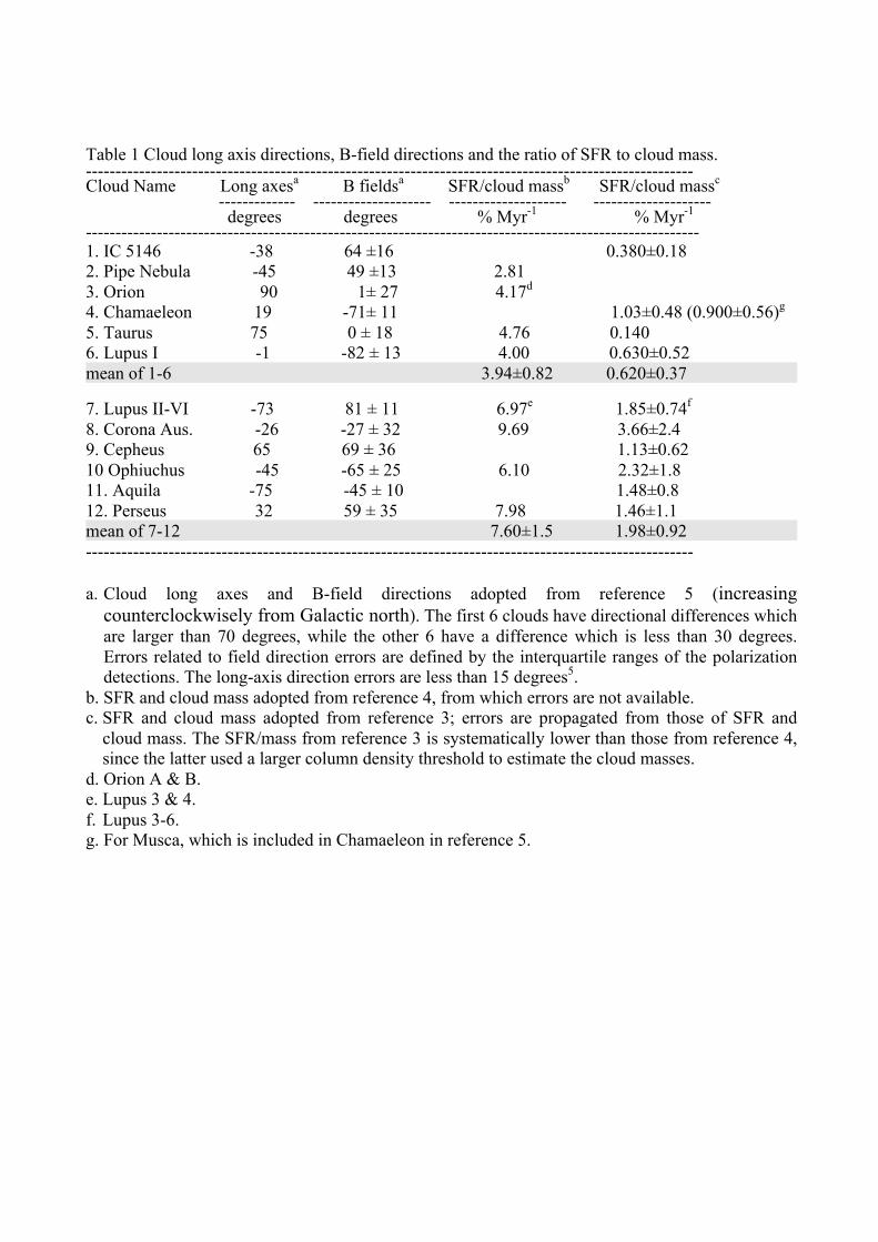
Table 1 Cloud long axis directions, B-field directions and the ratio of SFR to cloud mass. ------------------------------------------------------------------------------------------------------- Cloud Name Long axesa B fieldsa SFR/cloud massb SFR/cloud massc ------------- -------------------- -------------------- -------------------- degrees degrees % Myr-1 % Myr-1 -------------------------------------------------------------------------------------------------------- 1. IC 5146 -38 64 ±16 0.380±0.18 2. Pipe Nebula -45 49 ±13 2.81 3. Orion 90 1± 27 4.17d 4. Chamaeleon 19 -71± 11 1.03±0.48 (0.900±0.56)g 5. Taurus 75 0 ± 18 4.76 0.140 6. Lupus I -1 -82 ± 13 4.00 0.630±0.52 mean of 1-6 3.94±0.82 0.620±0.37 7. Lupus II-VI -73 81 ± 11 6.97e 1.85±0.74f 8. Corona Aus. -26 -27 ± 32 9.69 3.66±2.4 9. Cepheus 65 69 ± 36 1.13±0.62 10 Ophiuchus -45 -65 ± 25 6.10 2.32±1.8 11. Aquila -75 -45 ± 10 1.48±0.8 12. Perseus 32 59 ± 35 7.98 1.46±1.1 mean of 7-12 7.60±1.5 1.98±0.92 ------------------------------------------------------------------------------------------------------- a. Cloud long axes and B-field directions adopted from reference 5 (increasing
counterclockwisely from Galactic north). The first 6 clouds have directional differences which are larger than 70 degrees, while the other 6 have a difference which is less than 30 degrees. Errors related to field direction errors are defined by the interquartile ranges of the polarization detections. The long-axis direction errors are less than 15 degrees5.
b. SFR and cloud mass adopted from reference 4, from which errors are not available. c. SFR and cloud mass adopted from reference 3; errors are propagated from those of SFR and
cloud mass. The SFR/mass from reference 3 is systematically lower than those from reference 4, since the latter used a larger column density threshold to estimate the cloud masses.
d. Orion A & B. e. Lupus 3 & 4. f. Lupus 3-6. g. For Musca, which is included in Chamaeleon in reference 5.

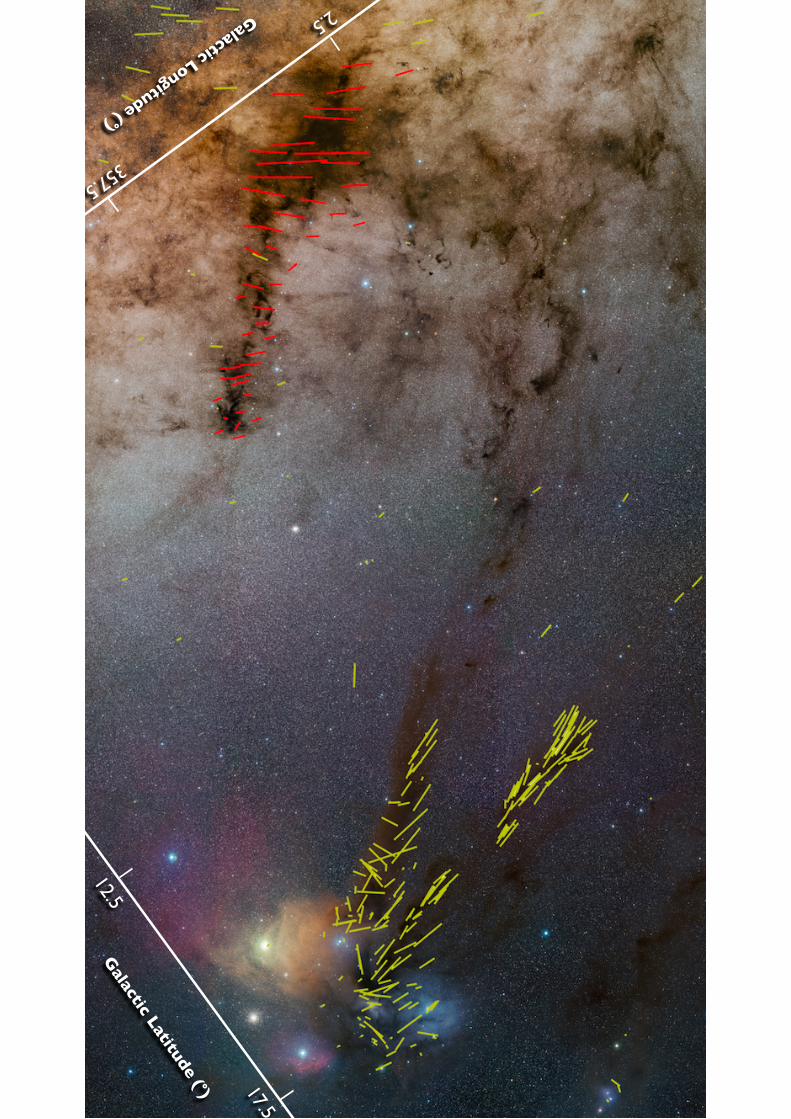
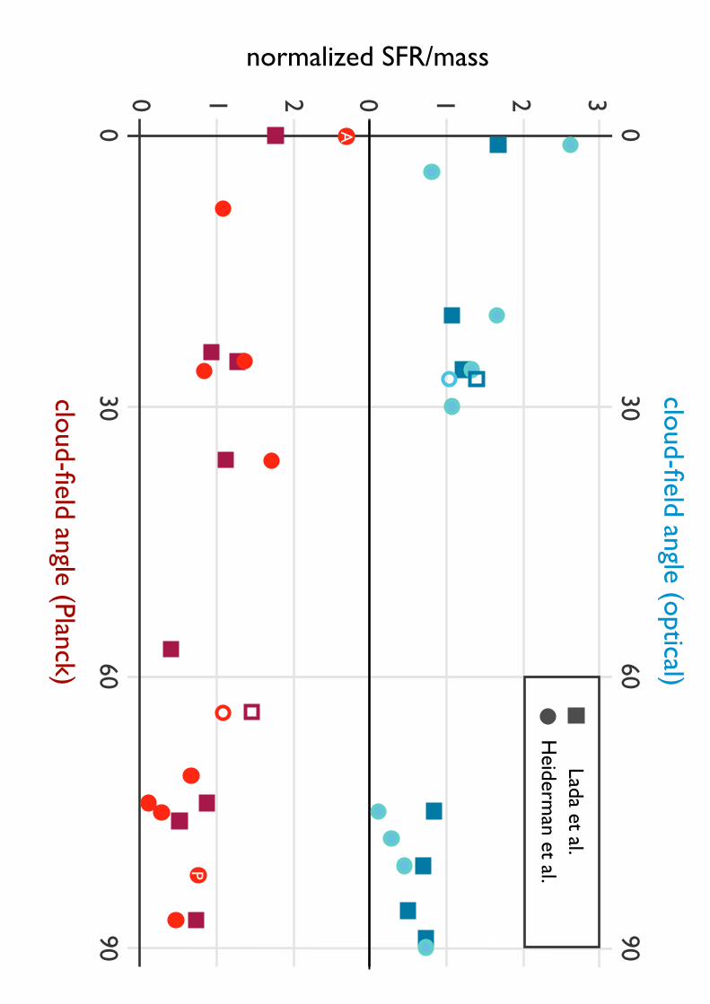
Figure 1 - Filamentary clouds and B-fields in the Pipe-Ophiuchus region. The dark lanes are clouds traced by the extinction of the background starlight (photo credit: Stéphane Guisard). The line segments indicate B-field directions inferred from the polarization of the background starlight. Pipe Nebula, overlapped with the red lines28, tends to be perpendicular to the B-fields. On the other hand, Ophiuchus cloud, covered by the yellow lines29, is largely aligned with the fields. They are not special cases from the Gould Belt, where most molecular clouds are elongated and tend to be aligned either parallel or perpendicular to local B-fields5. Figure 2 - SFR per unit mass versus cloud-field alignment for the Gould Belt clouds. The SFR and cloud mass are adopted from the surveys performed by Heiderman et al.3 and Lada et al.4 (Table I). For each survey, the SFR/mass is normalized to the mean. The cloud long axes and B-field directions based on optical data in the upper plot are adopted from Li et al.5 (Table I). In the lower plot, we replace the B-field directions from Li et al.5 with Planck 353 GHz polarization data30 (Methods; Supplementary Table 1). Perseus cloud, shown as hollow symbols, has significantly different mean field directions based on optical and Planck data (see the main text and Methods for discussion). The “alignment parameters” used in reference 30 are shown in Supplementary Figure 5 for the clouds noted as (for aligned) and (for perpendicular) to illustrate the connection between the two analyses. Figure 3 - Left: An illustration of how the magnetic flux of an elongated cloud can vary with the cloud-field alignment. A cross-section perpendicular to the B-field is highlighted for the cylindrical cloud when it is parallel (red) or perpendicular (green) to the local field. The area of each cross-section is shown below the cloud. Right: The distribution of mass-size relation, m(r), of the fragmentation from four Gould-Belt clouds21. Comparable to the left panel, the areas within the red dashed line or red shaded region are from small-angle clouds, based on the optical polarimetry data. The large-angle clouds, within the green dashed line or green shaded region, have an overall lower fragmented mass. The dotted dark lines are for references, which follow either m(r) µ r2 or m(r) µ r for an isothermal equilibrium sphere at 10K.

Acknowledgements The research was supported by Hong Kong Research Grant Council, projects T12/402/13N, ECS24300314 and GRF14600915; also by CUHK Direct Grant for Research, project 4053126 ‘Analyzing Simulation Data of Star Formation’. H.L. appreciates the conference “Star Formation in Different Environments 2016”, where the discussion, especially with Christopher Matzner and Juan Diego Soler, inspired the direction we present this work. Q.G. thanks Yi Wang for the discussion on Planck data analysis. Author contributions H.L. designed and executed the experiment. H.J. and X.F. were in charge of the statistical tests. Q.G. and Y.Z. were responsible for the Planck data analysis. Competing financial interests The authors declare no competing financial interests. Corresponding author Hua-bai Li
2.5 357.5
Galactic Longitude (°)
12.5 17.5
Galactic Latitude (°)
cloud-field angle (Planck)
normalized SFR/mass
0 30 60 90
3210210
0 30 60 90
cloud-field angle (optical)
Lada et al.H
eiderman et al.
A
P
B-field
{
ld
ldd2
π4
No.1,2010
MA
SS–SIZE
RE
LA
TIO
NFR
OM
CL
OU
DS
TO
CO
RE
S.II.435
Figure
1.Mass–size
relationsfor
theclouds
listedin
Table1.In
mostclouds,data
fromtw
odifferentobservationaltechniques
(e.g.,dustextinctionand
emission)
arecom
binedto
providea
comprehensive
pictureprobing
aw
iderange
ofspatialscales.Solid
blacklines
highlightcloudregions
containingthe
mostm
assivecloud
fragmentfound
forsmallradii.G
reenlines
startingin
circlesindicate
theglobalm
ass–sizerelations
discussedin
Section2.1.2.T
heother
dottedlines
givereference
mass–size
relationsas
discussedin
Section2.1.3.In
Orion
A,published
dataextracted
usingC
LU
MPFIN
D-like
approachesare
plotted(diam
ondsm
arkSC
UB
Adata,
crossesindicate
CO
observations)instead
ofusing
thecontour-based
scheme
employed
here.Further,thetriangle
indicatesthe
large-scaleO
rionA
extinctionm
assm
easurementdiscussed
inthe
text.
PipeN
ebulaare
examined
here.Asa
generalreferenceto
cloudsalso
forming
high-mass
stars,w
einclude
theO
rionA
cloud.T
hen,them
orerem
oteG
10.15−0.34
(hereafterG10;∼
2.1
kpc)and
G11.11−
0.12com
plexes(hereafter
G11;
∼3.6
kpc)are
studiedto
builda
firstbridge
toward
thestudy
ofrelatively
distantsitesof
high-mass
starform
ation(see
Pillaietal.2007fordistances
andreferences;G
10is
furtherdiscussedby
Wood
&C
hurchwell
1989and
Thom
psonet
al.2006,
while
Pillaiet
al.2006b
studyG
11).N
otethat
G11
isan
InfraredD
arkC
loud(IR
DC
;seeM
entenet
al.2005and
Beuther
etal.2007forreview
s).A
datasum
mary
forour
sample
isprovided
inTable
1.This
includesparam
etersused
forthesource
extraction.
2.2.1.Data
andA
nalysis
The
extinctionm
apanalysis
forO
phiuchus(R
idgeet
al.2006)and
thePipe
Nebula
(Lom
bardietal.2006)isanalogous
tothe
onefor
thePerseus
cloudcarried
outin
PaperI.
The
visualextinction
inthe
PipeN
ebulam
apis
reducedby
1.34
mag
(reductionof
0.15
mag
inA
K ),following
theanalysis
byL
ombardi
etal.
(2008).For
Taurus,w
euse
them
apby
Row
les&
Froebrich(2009).
Itsresolution
variesthroughout
them
ap.T
hisis
analogousto
aregion-dependent
smoothing,
which
may
affectm
assestim
ates(Section
4.1in
PaperI).W
ethus
usethis
map
with
caution.In
Taurus(K
auffmann
etal.
2008)andO
phiuchus(E
nochetal.2007),the
processingofthe
dustem
issionm
apsfollow
sthe
PerseusB
olocamanalysis
ofPaperI.N
otethatthe
TaurusM
AM
BO
maps
donotcoverallof
thecloud
andm
aytherefore
givea
biasedview
ofthedense
coreconditions.Pipe
Nebula
regionsw
ithhigh
column
densitym
ustbe
probedin
detail.Todo
this,we
includea
SCU
BA
map
forB
68(A
lvesetal.2001),w
hichis
kindlyprovided
byJ.A
lves.R
oman-Z
unigaet
al.(2009)m
appedthe
Pipe’sB
59region
inextinction.W
eprocess
thesem
apsusing
ouranalysis
scheme.
Forall
sources,Table
1lists
thefree
parameters
usedin
oursource
extractionalgorithm
.T
heresulting
mass–size
relationsform
partof
Figure1.To
illustratesom
easpects
ofthe
spatialcloud
structure,Figure1
highlights(in
black)foreverycloud
them
ass–sizeevolution
ofthe
most
massive
fragment
foundat
small
radii.N
otethat,
inTaurus
andthe
PipeN
ebula,thesefragm
entsdo
notform
partofthe
largestcloudfragm
entsfound
inthe
maps.
InO
rionA
,nodata
suitedfora
reliabledendrogram
structureanalysis
ofcolumn
densitiesis
yetavailable.Instead,we
usethe
Row
les&
Froebrich(2009)
extinctionm
apsto
derivea
singlem
assand
sizem
easurement
onthe
largestscales
probedby
thatmap.O
nsm
allerscales,the
extinctionm
apis
notreliablebecause
oftoo
fewbackground
sources.Forreference,w
ealso
plotmass
andsize
measurem
entsfor
13CO
clumps
inO
rion,aspublished
elsewhere
(Bally
etal.1987;theirTable
1,plustext
statements).T
hesedata
are,however,notused
inthe
quantitativeanalysis.
At
smaller
scales,w
efold
inpublished
datafrom
PerseusOph
PipeTaurus
No.1,2010
MA
SS–SIZE
RE
LA
TIO
NFR
OM
CL
OU
DS
TO
CO
RE
S.II.435
Figure
1.Mass–size
relationsfor
theclouds
listedin
Table1.In
mostclouds,data
fromtw
odifferentobservationaltechniques
(e.g.,dustextinctionand
emission)
arecom
binedto
providea
comprehensive
pictureprobing
aw
iderange
ofspatialscales.Solid
blacklines
highlightcloudregions
containingthe
mostm
assivecloud
fragmentfound
forsmallradii.G
reenlines
startingin
circlesindicate
theglobalm
ass–sizerelations
discussedin
Section2.1.2.T
heother
dottedlines
givereference
mass–size
relationsas
discussedin
Section2.1.3.In
Orion
A,published
dataextracted
usingC
LU
MPFIN
D-like
approachesare
plotted(diam
ondsm
arkSC
UB
Adata,
crossesindicate
CO
observations)instead
ofusing
thecontour-based
scheme
employed
here.Further,thetriangle
indicatesthe
large-scaleO
rionA
extinctionm
assm
easurementdiscussed
inthe
text.
PipeN
ebulaare
examined
here.Asa
generalreferenceto
cloudsalso
forming
high-mass
stars,w
einclude
theO
rionA
cloud.T
hen,them
orerem
oteG
10.15−0.34
(hereafterG10;∼
2.1
kpc)and
G11.11−
0.12com
plexes(hereafter
G11;
∼3.6
kpc)are
studiedto
builda
firstbridge
toward
thestudy
ofrelatively
distantsitesof
high-mass
starform
ation(see
Pillaietal.2007fordistances
andreferences;G
10is
furtherdiscussedby
Wood
&C
hurchwell
1989and
Thom
psonet
al.2006,
while
Pillaiet
al.2006b
studyG
11).N
otethat
G11
isan
InfraredD
arkC
loud(IR
DC
;seeM
entenet
al.2005and
Beuther
etal.2007forreview
s).A
datasum
mary
forour
sample
isprovided
inTable
1.This
includesparam
etersused
forthesource
extraction.
2.2.1.Data
andA
nalysis
The
extinctionm
apanalysis
forO
phiuchus(R
idgeet
al.2006)and
thePipe
Nebula
(Lom
bardietal.2006)isanalogous
tothe
onefor
thePerseus
cloudcarried
outin
PaperI.
The
visualextinction
inthe
PipeN
ebulam
apis
reducedby
1.34
mag
(reductionof
0.15
mag
inA
K ),following
theanalysis
byL
ombardi
etal.
(2008).For
Taurus,w
euse
them
apby
Row
les&
Froebrich(2009).
Itsresolution
variesthroughout
them
ap.T
hisis
analogousto
aregion-dependent
smoothing,
which
may
affectm
assestim
ates(Section
4.1in
PaperI).W
ethus
usethis
map
with
caution.In
Taurus(K
auffmann
etal.
2008)andO
phiuchus(E
nochetal.2007),the
processingofthe
dustem
issionm
apsfollow
sthe
PerseusB
olocamanalysis
ofPaperI.N
otethatthe
TaurusM
AM
BO
maps
donotcoverallof
thecloud
andm
aytherefore
givea
biasedview
ofthedense
coreconditions.Pipe
Nebula
regionsw
ithhigh
column
densitym
ustbe
probedin
detail.Todo
this,we
includea
SCU
BA
map
forB
68(A
lvesetal.2001),w
hichis
kindlyprovided
byJ.A
lves.R
oman-Z
unigaet
al.(2009)m
appedthe
Pipe’sB
59region
inextinction.W
eprocess
thesem
apsusing
ouranalysis
scheme.
Forall
sources,Table
1lists
thefree
parameters
usedin
oursource
extractionalgorithm
.T
heresulting
mass–size
relationsform
partof
Figure1.To
illustratesom
easpects
ofthe
spatialcloud
structure,Figure1
highlights(in
black)foreverycloud
them
ass–sizeevolution
ofthe
most
massive
fragment
foundat
small
radii.N
otethat,
inTaurus
andthe
PipeN
ebula,thesefragm
entsdo
notform
partofthe
largestcloudfragm
entsfound
inthe
maps.
InO
rionA
,nodata
suitedfora
reliabledendrogram
structureanalysis
ofcolumn
densitiesis
yetavailable.Instead,we
usethe
Row
les&
Froebrich(2009)
extinctionm
apsto
derivea
singlem
assand
sizem
easurement
onthe
largestscales
probedby
thatmap.O
nsm
allerscales,the
extinctionm
apis
notreliablebecause
oftoo
fewbackground
sources.Forreference,w
ealso
plotmass
andsize
measurem
entsfor
13CO
clumps
inO
rion,aspublished
elsewhere
(Bally
etal.1987;theirTable
1,plustext
statements).T
hesedata
are,however,notused
inthe
quantitativeanalysis.
At
smaller
scales,w
efold
inpublished
datafrom
Supplementary Information
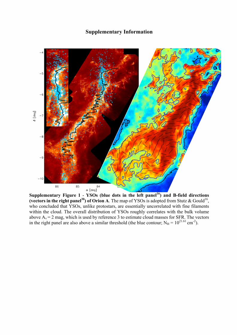
Supplementary Figure 1 - YSOs (blue dots in the left panel16) and B-field directions (vectors in the right panel30) of Orion A. The map of YSOs is adopted from Stutz & Gould16, who concluded that YSOs, unlike protostars, are essentially uncorrelated with fine filaments within the cloud. The overall distribution of YSOs roughly correlates with the bulk volume above Av = 2 mag, which is used by reference 3 to estimate cloud masses for SFR. The vectors in the right panel are also above a similar threshold (the blue contour; NH = 1021.61 cm-2).

Supplementary Figure 2 – An illustration of how the polarization data from reference 30 is adopted in this study. Left: Adopted from Planck Collaboration30 are the column density maps, log
10(NH/cm2), overlapped with magnetic field directions (vectors) inferred from the 353
GHz polarization data. Taurus and CrA are shown as examples. The thresholds of intermediate density30 are indicated by the blue contours. Right: We collected the Planck 353 GHz polarization data above the intermediate-density thresholds and calculated the mean B-field directions. Another example, Orion A, is shown in Supplementary Figure 1 (right panel). The maps of the rest 11 clouds are given in Supplementary Figure 3.
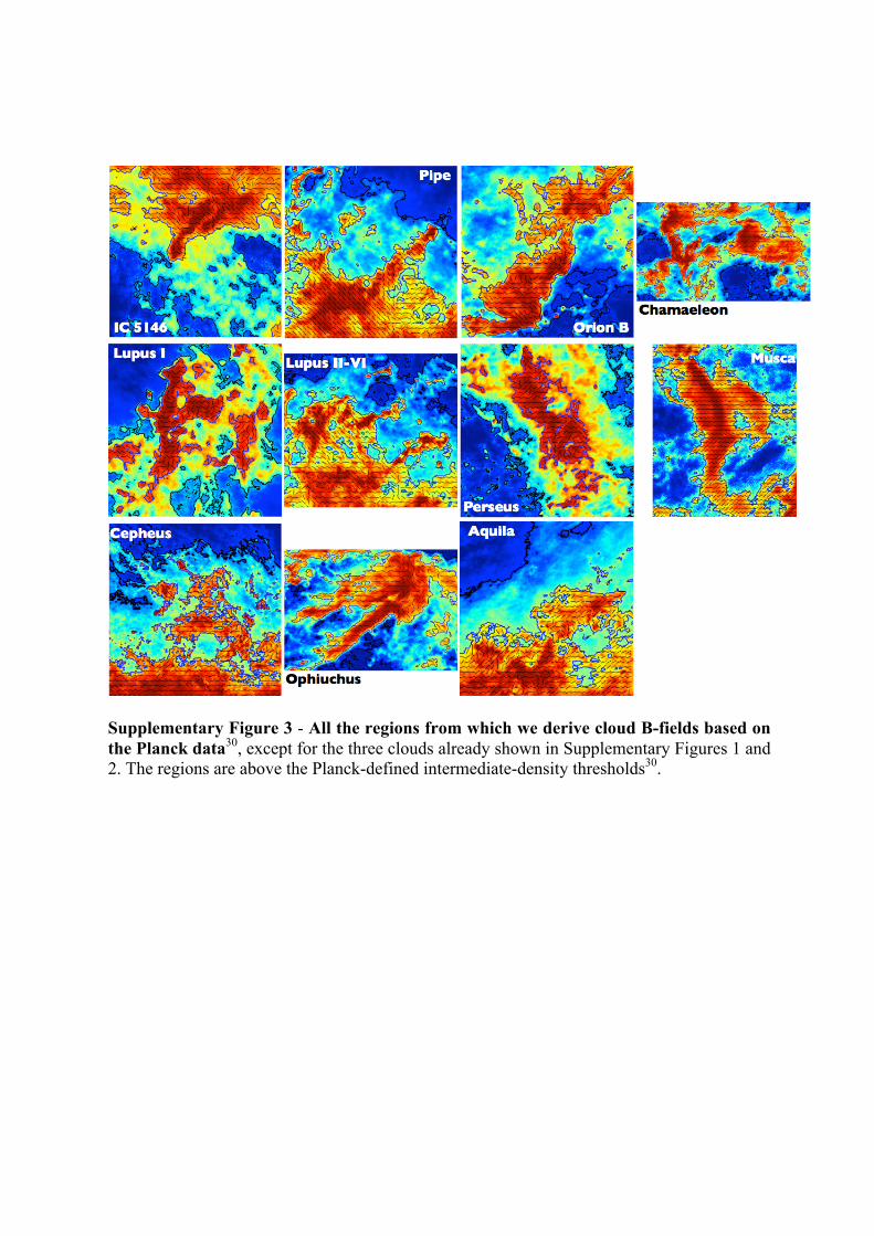
Supplementary Figure 3 - All the regions from which we derive cloud B-fields based on the Planck data30, except for the three clouds already shown in Supplementary Figures 1 and 2. The regions are above the Planck-defined intermediate-density thresholds30.
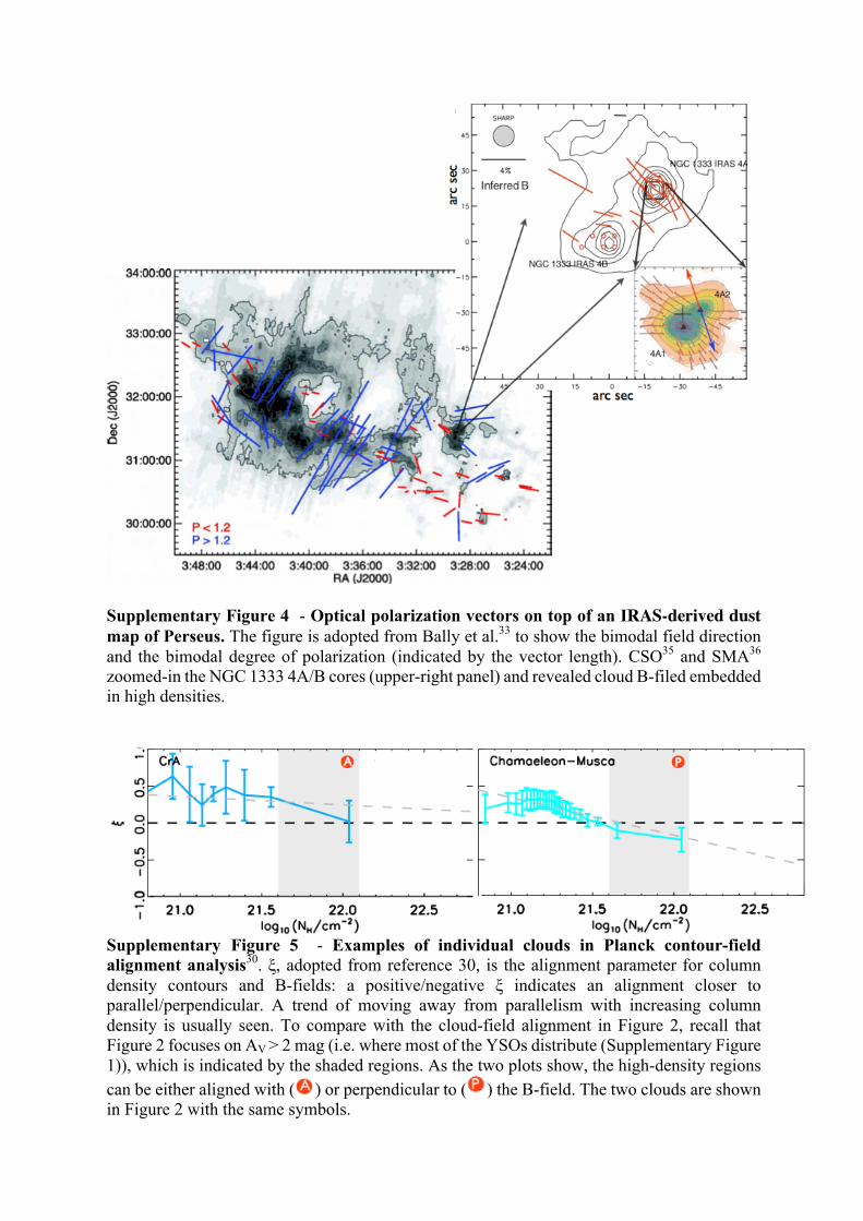
Supplementary Figure 4 - Optical polarization vectors on top of an IRAS-derived dust map of Perseus. The figure is adopted from Bally et al.33 to show the bimodal field direction and the bimodal degree of polarization (indicated by the vector length). CSO35 and SMA36 zoomed-in the NGC 1333 4A/B cores (upper-right panel) and revealed cloud B-filed embedded in high densities.
Supplementary Figure 5 - Examples of individual clouds in Planck contour-field alignment analysis30. ξ, adopted from reference 30, is the alignment parameter for column density contours and B-fields: a positive/negative ξ indicates an alignment closer to parallel/perpendicular. A trend of moving away from parallelism with increasing column density is usually seen. To compare with the cloud-field alignment in Figure 2, recall that Figure 2 focuses on AV > 2 mag (i.e. where most of the YSOs distribute (Supplementary Figure 1)), which is indicated by the shaded regions. As the two plots show, the high-density regions can be either aligned with ( ) or perpendicular to ( ) the B-field. The two clouds are shown in Figure 2 with the same symbols.
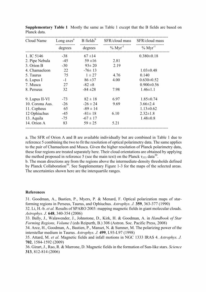
Supplementary Table 1 Mostly the same as Table 1 except that the B fields are based on Planck data. ------------------------------------------------------------------------------------------------------- Cloud Name Long axesa B fieldsb SFR/cloud mass SFR/cloud mass -------------- ------------- -------------------- -------------------- degrees degrees % Myr-1 % Myr-1 -------------------------------------------------------------------------------------------------------- 1. IC 5146 -38 67 ±14 0.380±0.18 2. Pipe Nebula -45 59 ±16 2.81 3. Orion B -30 93± 20 2.19 4. Chamaeleon 22 -76± 13 1.03±0.48 5. Taurus 75 1 ± 27 4.76 0.140 6. Lupus I -1 86 ±37 4.00 0.630±0.52 7. Musca 27 -82 ±8 0.900±0.56 8. Perseus 32 -84 ±28 7.98 1.46±1.1 9. Lupus II-VI -73 82 ± 18 6.97 1.85±0.74 10. Corona Aus. -26 -26 ± 24 9.69 3.66±2.4 11. Cepheus 65 -89 ± 14 1.13±0.62 12 Ophiuchus -45 -81± 18 6.10 2.32±1.8 13. Aquila -75 -67 ± 17 1.48±0.8 14. Orion A 83 59 ± 25 5.21 ------------------------------------------------------------------------------------------------------- a. The SFR of Orion A and B are available individually but are combined in Table 1 due to reference 5 combining the two to fit the resolution of optical polarimetry data. The same applies to the pair of Chamaeleon and Musca. Given the higher resolution of Planck polarimetry data, these four regions are treated separately here. Their cloud orientations are obtained by applying the method proposed in reference 5 (see the main text) on the Planck τ353 data30. b. The mean directions are from the regions above the intermediate-density thresholds defined by Planck Collaboration30. See Supplementary Figure 1-3 for the maps of the selected areas. The uncertainties shown here are the interquartile ranges.
References 31. Goodman, A., Bastien, P., Myers, P. & Menard, F. Optical polarization maps of star-forming regions in Perseus, Taurus, and Ophiuchus. Astrophys. J. 359, 363-377 (1990) 32. Li, H.-b. et al. Results of SPARO 2003: mapping magnetic fields in giant molecular clouds. Astrophys. J. 648, 340-354 (2006) 33. Bally, J., Walawender, J., Johnstone, D., Kirk, H. & Goodman, A. in Handbook of Star Forming Regions, Volume I (eds Reipurth, B.) 308 (Astron. Soc. Pacific Press, 2008) 34. Arce, H., Goodman, A., Bastien, P., Manset, N. & Sumner, M. The polarizing power of the interstellar medium in Taurus. Astrophys. J. 499, L93-L97 (1998) 35. Attard, M. et al. Magnetic fields and infall motions in NGC 1333 IRAS 4. Astrophys. J. 702, 1584-1592 (2009) 36. Girart, J., Rao, R. & Marrone, D. Magnetic fields in the formation of Sun-like stars. Science 313, 812-814 (2006)