The Linear Frame Element - University of British Columbiainrisk.sites.olt.ubc.ca/files/2012/11/The-Linear-Frame-Element.pdfThe Linear Frame Element Updated December 24, ... body motion

Professor Terje Haukaas University of British Columbia, Vancouver www.inrisk.ubc.ca

The Linear Frame Element Updated December 24, 2014 Page 1

The Linear Frame Element The beam element, called frame element here to emphasize that it can be used to model columns too, is by far the most popular finite element in structural analysis. A variety of alternatives exist, from 2D Euler-Bernoulli beams to 3D beams with torsion, shear deformation, and geometric stiffness contributions. Figure 1 shows four element configurations related to 2D structural analysis with axial and bending deformation. The two lower-most drawings show “basic” configurations; they have DOFs that are sufficient only for describing deformation, not rigid-body motions. What distinguishes the two lower-most configurations is inclusion of axial deformation. The upper-most drawings in Figure 1 show the “local” configuration, also with and without axial deformation. These are capable of describing any deformation pattern, including rigid body motion. Transformation from the local configuration to a global structural coordinate system is addressed in the document on the computational stiffness method.

Figure 1: Beam element configurations for 2D structural analysis.

The stiffness matrix for each element configuration in Figure 1 is known from the classical stiffness method. For reference, they are:

Kb =

4EIL

2EIL

2EIL

4EIL

⎡

⎣

⎢⎢⎢⎢

⎤

⎦

⎥⎥⎥⎥

(1)

2 1

3

4

3 1

2

z, w

x, u 2 1

4

5 2

1 3 6

z, w

x, u

x, u

x, u

z, w z, w



Kb =

EAL

0 0

0 4EIL

2EIL

0 2EIL

4EIL

⎡

⎣

⎢⎢⎢⎢⎢⎢⎢

⎤

⎦

⎥⎥⎥⎥⎥⎥⎥

(2)

Kl =

12EIL3

−6EIL2

−12EIL3

−6EIL2

−6EIL2

4EIL

6EIL2

2EIL

−12EIL3

6EIL2

12EIL3

6EIL2

−6EIL2

2EIL

6EIL2

4EIL

⎡

⎣

⎢⎢⎢⎢⎢⎢⎢⎢⎢⎢

⎤

⎦

⎥⎥⎥⎥⎥⎥⎥⎥⎥⎥

(3)

Kl =

EAL

0 0 −EAL

0 0

0 12EIL3

−6EIL2

0 −12EIL3

−6EIL2

0 −6EIL2

4EIL

0 6EIL2

2EIL

−EAL

0 0 EAL

0 0

0 −12EIL3

6EIL2

0 12EIL3

6EIL2

0 −6EIL2

2EIL

0 6EIL2

4EIL

⎡

⎣

⎢⎢⎢⎢⎢⎢⎢⎢⎢⎢⎢⎢⎢⎢⎢⎢

⎤

⎦

⎥⎥⎥⎥⎥⎥⎥⎥⎥⎥⎥⎥⎥⎥⎥⎥

(4)

To illustrate the finite element method, consider the 2D beam element in its basic configuration, without axial deformations. It is selected to employ the weak form of the BVP, with the principle of virtual displacements as a starting point. To this end, consider the equality of internal and external virtual work as a starting point:

δWint = δWext (5)

In particular, the principle of virtual displacements reads

σ δε dVV∫ = qz δwdx

0

L

∫ (6)

Substitution of material law yields



Eεδε dVV∫ = qz δwdx

0

L

∫ (7)

Substitution of kinematics yields

E ⋅ z2 ⋅w ''δw ''dVV∫ = qz δwdx

0

L

∫ (8)

Separation of the left-hand side integral into a cross-section integral and a longitudinal integral yields

EI ⋅w ''δw ''dx0

L

∫ = qz δwdx0

L

∫ (9)

This is the weak form of the BVP for beam bending. The all-important discretization of this problem by means of shape functions follows. The element has two basic DOFs related to bending. Imagine the element in a horizontal position with the coordinate x running from 0 at the left end to L at the right end. Let the clockwise rotation of the left end be denoted u1 and let the clockwise rotation at the right end be denoted u2. Third-order polynomial shape functions are possible, given two rotational DOFs and zero displacement at the element ends. Consequently, the shape functions are:

w(x) = Nu = N1(x) N2 (x)⎡⎣

⎤⎦

u1u2

⎧⎨⎪

⎩⎪

⎫⎬⎪

⎭⎪ (10)

where

N1(x) = −

1L2x3 +

2Lx2 − x

N2 (x) = −1L2x3 +

1Lx2

(11)

Substitution into the weak form yields

EI ⋅ N ''u( ) ⋅ N ''δu( ) dx0

L

∫ − qz Nδu( ) dx0

L

∫ = 0 (12)

where δu is the virtual nodal deformations because the virtual displacements are discretized by the same shape functions as the actual displacements. Rearranging yields

δu EI ⋅N ''TN '' dx0

L

∫⎡⎣⎢⎤⎦⎥

u − qz NT dx

0

L

∫( ) = 0 (13)

Furthermore, because the virtual displacements are arbitrary the parenthesis must be zero for this equation to be generally valid. Consequently, it is rewritten

EI ⋅N ''T N ''dx0

L

∫⎡

⎣⎢

⎤

⎦⎥

Stiffness matrix, K

u = qzNdx0

L

∫Load vector, F

(14)



where the stiffness matrix and load vector are identified. Again it is noted that the finite element method yields integral expressions for the stiffness matrix and the load vector. Substitution of Eq. (11) into Eq. (14) and assuming that the distributed element load is uniform yields

4EIL

2EIL

2EIL

4EIL

⎡

⎣

⎢⎢⎢⎢

⎤

⎦

⎥⎥⎥⎥

u1u2

⎧⎨⎪

⎩⎪

⎫⎬⎪

⎭⎪=

−qzL

2

12qzL

2

12

⎧

⎨⎪⎪

⎩⎪⎪

⎫

⎬⎪⎪

⎭⎪⎪

(15)

This stiffness matrix is equal to that of the classical stiffness method because the third-order polynomial shape functions match the solution of the differential equation for beam bending. Under such circumstances the finite element method is exact. Notice that the right-hand side load vector has the correct sign for upward-acting qz and clockwise rotation DOFs.

Shear Deformation The inclusion of shear deformation in the stiffness matrix for beam elements is possible by employing the unit virtual load method to establish the flexibility matrix, followed by inversion to obtain the stiffness matrix. This takes place in the basic element configuration. As a starting point, recall that the a stiffness coefficient kij is “force along degree of freedom number i due to a unit displacement/rotation along degree of freedom number j.” However, the unit virtual load method yields deformations, not forces. For that reason it is convenient to first establish the flexibility coefficients fij instead of stiffness coefficients kij. Subsequently, the flexibility matrix is inverted to obtain the stiffness matrix. Figure 2 shows the virtual and real section force diagrams used to obtain f11, f12, f21, and f22, where fij is the displacement or rotation along degree of freedom number i due to a unit force along degree of freedom number j. Each flexibility coefficient is computed by evaluating the virtual work integral

fij =M ⋅δMEI0

L

∫ dx + V ⋅δVGAv0

L

∫ dx (16)

By employing the “quick integration” formulas from the unit virtual work method, the following results are obtained:

f11 =13EI

⋅1⋅1⋅L + 1GAv

⋅ − 1L

⎛⎝⎜

⎞⎠⎟ ⋅ − 1

L⎛⎝⎜

⎞⎠⎟ ⋅L = L

3EI+ 1GAvL

(17)

f21 = − 16EI

⋅1⋅1⋅L + 1GAv

⋅ − 1L

⎛⎝⎜

⎞⎠⎟ ⋅ − 1

L⎛⎝⎜

⎞⎠⎟ ⋅L = − L

6EI+ 1GAvL

(18)

f12 = − 16EI

⋅1⋅1⋅L + 1GAv

⋅ − 1L

⎛⎝⎜

⎞⎠⎟ ⋅ − 1

L⎛⎝⎜

⎞⎠⎟ ⋅L = − L

6EI+ 1GAvL

(19)



f22 =13EI

⋅1⋅1⋅L + 1GAv

⋅ − 1L

⎛⎝⎜

⎞⎠⎟ ⋅ − 1

L⎛⎝⎜

⎞⎠⎟ ⋅L = L

3EI+ 1GAvL

(20)

Figure 2: Beam cases for virtual work computations.

The results are summarized by the equation

θ1θ2

⎡

⎣⎢⎢

⎤

⎦⎥⎥=

f11 f12f21 f22

⎡

⎣⎢⎢

⎤

⎦⎥⎥

M1

M 2

⎡

⎣⎢⎢

⎤

⎦⎥⎥

(21)

By defining the auxiliary coefficient

α =12EIGAvL

2 (22)

and summarizing the above results, the flexibility matrix in the basic element configuration is:

f12

f22

f11

f21

Real:

1

1

–1/L

M

V

Virtual:

1

1

–1/L

δM

δV

Real:

1

1

–1/L

M

V

Virtual:

–1/L

δM

δV

1

1 Virtual:

–1/L

δM

δV

1

1

Real:

1

1

–1/L

M

V

Virtual:

1

1

–1/L

δM

δV

Real:

1

1

–1/L

M

V



θ1θ2

⎡

⎣⎢⎢

⎤

⎦⎥⎥= L6EI

⋅2 + α

2⎛⎝⎜

⎞⎠⎟ − 1− α

2⎛⎝⎜

⎞⎠⎟

− 1− α2

⎛⎝⎜

⎞⎠⎟ 2 + α

2⎛⎝⎜

⎞⎠⎟

⎡

⎣

⎢⎢⎢⎢⎢

⎤

⎦

⎥⎥⎥⎥⎥

M1

M 2

⎡

⎣⎢⎢

⎤

⎦⎥⎥

(23)

In passing, it is noted that the expression for a for a rectangular cross-section with zero Poisson’s ratio is

α =12 ⋅E ⋅ b ⋅h

3

12E2⋅ 56⋅b ⋅h ⋅L2

= 125⋅ hL

⎛⎝⎜

⎞⎠⎟2

(24)

which reasonably suggests that beams with higher h/L ratio exhibits more shear deformation. Next, inversion of the flexibility matrix in Eq. (23) yields the stiffness matrix in the basic configuration, modified with shear deformation:

Kb =EI

(1+α )L⋅

4 +α( ) 2 −α( )2 −α( ) 4 +α( )

⎡

⎣⎢⎢

⎤

⎦⎥⎥

(25)

Transformation to the local coordinate system with the transformation matrix that is shown in the document on the computational stiffness method yields:

Kl =1

(1+α )⋅

12EIL3

−6EIL2

−12EIL3

−6EIL2

−6EIL2

(4 +α ) ⋅EIL

6EIL2

(2 −α ) ⋅EIL

−12EIL3

6EIL2

12EIL3

6EIL2

−6EIL2

(2 −α ) ⋅EIL

6EIL2

(4 +α ) ⋅EIL

⎡

⎣

⎢⎢⎢⎢⎢⎢⎢⎢⎢⎢

⎤

⎦

⎥⎥⎥⎥⎥⎥⎥⎥⎥⎥

(26)

To ease the extraction of values from Eq. (26) in hand calculations, the stiffness coefficients in Eq. (26) are provided for two fundamental beam cases in Figure 3.



Figure 3: Amendment of fundamental beam cases with shear deformation terms.

Geometric Stiffness Significant axial compressive force in a beam-column member reduces its lateral stiffness. Conversely, axial tension force increases the lateral stiffness. This change in stiffness due to axial force is called geometric stiffness, and is often referred to a “P-delta effects.” In this section, the finite element approach is utilized to amend the stiffness matrix for frame members. The resulting geometric stiffness matrix is approximate because the shape functions differ from the solution to the differential equation. The expression for the exact geometric stiffness matrix is more complicated, and is presented under the theory for beam members with axial force. In the following, the principle of virtual displacements is first employed with polynomial shape functions. Start by considering the differential equation for beam bending, amended with the P-delta effect. In the absence of distributed load q, the weighted and integrated version reads

EI ⋅w ''''+ P ⋅w ''( )δwdx0

L

∫ = 0 (27)

Integration by parts and cancelling boundary terms yield

EI ⋅w ''δw ''dx0

L

∫ − P ⋅w 'δw 'dx0

L

∫ = 0 (28)

Discretization of the real and virtual displacement fields by shape functions, i.e., w(x)=Nu and δw(x)=Nδu, where the vector u collects the displacements along the degrees of freedom, yields

EI ⋅N ''T ⋅N ''dx0

L

∫ − P ⋅ N 'T ⋅N 'dx0

L

∫kG

⎛

⎝

⎜⎜⎜

⎞

⎠

⎟⎟⎟⋅u = 0 (29)

(2 −α ) ⋅EI(1+α ) ⋅L

(4 +α ) ⋅EI(1+α ) ⋅L

6EI(1+α ) ⋅L2

− 6EI(1+α ) ⋅L2

− 6EI(1+α ) ⋅L2

− 6EI(1+α ) ⋅L2

− 12EI(1+α ) ⋅L3

12EI(1+α ) ⋅L3

θ = 1.0

Δ = 1.0



where the geometric stiffness matrix, kG, is defined. Two paths can now be followed to obtain the geometric stiffness matrix in the local element configuration. Because the basic configuration neglects rigid-body movement of the element, using the shape functions for that configuration will miss the “P/L terms.” In other words, the P-delta effects associated with rigid-body movement of the element will be missed if the integral in Eq. (29) is conducted in the basic element configuration. For that reason, the following third-order polynomial shape functions for the beam element in the local configuration are employed:

N1(x) =2x3

L3− 3x

2

L2+1

N2 (x) = − x3

L2+ 2x

2

L− x

N3(x) = − 2x3

L3+ 3x

2

L2

N4 (x) = − x3

L2+ x

2

L

(30)

As a result, the following total stiffness matrix is obtained:

k =

12EIL3

− 6EIL2

−12EIL3

− 6EIL2

− 6EIL2

4EIL

6EIL2

2EIL

−12EIL3

6EIL2

12EIL3

6EIL2

− 6EIL2

2EIL

6EIL2

4EIL

⎡

⎣

⎢⎢⎢⎢⎢⎢⎢⎢⎢⎢

⎤

⎦

⎥⎥⎥⎥⎥⎥⎥⎥⎥⎥

− P ⋅

65L

− 110

− 65L

− 110

− 110

2L15

110

− L30

− 65L

110

65L

110

− 110

− L30

110

2L15

⎡

⎣

⎢⎢⎢⎢⎢⎢⎢⎢⎢⎢

⎤

⎦

⎥⎥⎥⎥⎥⎥⎥⎥⎥⎥

kG! "###### $######

(31)

If the integration had been conducted in the basic configuration, as mentioned above, it would be necessary to add the “P/L terms” to the result:

kG = P ⋅

15L

− 110

− 15L

− 110

− 110

2L15

110

− L30

− 15L

110

15L

110

− 110

− L30

110

2L15

⎡

⎣

⎢⎢⎢⎢⎢⎢⎢⎢⎢⎢

⎤

⎦

⎥⎥⎥⎥⎥⎥⎥⎥⎥⎥

+

PL

0 − PL

0

0 0 0 0

− PL

0 PL

0

0 0 0 0

⎡

⎣

⎢⎢⎢⎢⎢⎢⎢

⎤

⎦

⎥⎥⎥⎥⎥⎥⎥

(32)

To ease the extraction of values from Eq. (31) in hand calculations, the stiffness coefficients in Eq. (31) are provided for two fundamental beam cases in Figure 4.



Figure 4: Amendment of fundamental beam cases with geometric stiffness terms.

Exact Geometric Stiffness Matrix The geometric stiffness matrix in Eq. (31) is approximate because polynomial shape functions are employed while the solution above contains trigonometric functions. As an alternative, column by column of the exact stiffness matrix can be established by solving the differential equation for this problem, which is provided in the document on beam members with axial force. According to the classical stiffness method, the columns of the stiffness matrix are established by setting the degrees of freedom shown in Figure 5 equal to one, one at a time.

Figure 5: Degrees of freedom for beam element.

The first column of the stiffness matrix is obtained by setting u1=1 and u2=u3=u4=0 and computing the force along each degree of freedom:

F1 = V (0) = EI ⋅w '''(0)F2 = M (0) = EI ⋅w ''(0)F3 = −V (L) = −EI ⋅w '''(L)F4 = −M (L) = −EI ⋅w ''(L)

(33)

To simplify expressions, R.K. Livesley introduced the following auxiliary functions in his book entitled “Matrix Methods of Structural Analysis” published by Pergamon Press in Oxford, UK in 1975:

2EIL

+ PL30

4EIL

! 2PL15

6EIL2

! P10

! 6EIL2

+ P10

! 6EIL2

+ P10

! 6EIL2

+ P10

!12EIL3

+ 6P5L

12EIL3

! 6P5L

! = 1.0

! = 1.0

u4

u3 u1

u2



φ1 =β

tan(β)

φ2 =13⋅β 2

1−φ1

φ3 =14⋅φ1 +

34⋅φ2

φ4 = −12⋅φ1 +

32⋅φ2

φ5 = φ1 ⋅φ2

(34)

where

β =L2⋅

PEI

(35)

which leads to the following exact stiffness matrix, including both elastic stiffness and geometric stiffness:

K =2EIL3

⋅

6φ5 −3Lφ2 −6φ5 −3Lφ2−3Lφ2 2L2φ3 3Lφ2 L2φ4−6φ5 3Lφ2 6φ5 3Lφ2−3Lφ2 L2φ4 −3Lφ2 2L2φ3

⎡

⎣

⎢⎢⎢⎢⎢

⎤

⎦

⎥⎥⎥⎥⎥

(36)

Torsion While other documents describe the theory of St. Venant torsion and warping torsion, the stiffness matrix for a beam element with torsional DOFs is presented here. First it is noted that elements that only carry torque by St. Venant torsion have a rather simple stiffness matrix. In fact, the solution to the differential equation for St. Venant torsion yields

φ = TGJ

⋅L (37)

for an element with length L subjected to constant torque, T. This immediately produces the following stiffness matrix for St. Venant torsion:

kSt .V . =

GJL

−GJL

−GJL

GJL

⎡

⎣

⎢⎢⎢⎢

⎤

⎦

⎥⎥⎥⎥

(38)

The more general element carries torque with both shear and axial stresses, i.e., both St. Venant torsion and warping torsion. For this situation, consider the full set of DOFs shown in Figure 6. Two of the DOFs represent ordinary rotation around the x-axis, while



the other two represent warping deformation. In particular, the DOFs written in terms of deformation are:

u =

u1u2u3u4

⎧

⎨

⎪⎪

⎩

⎪⎪

⎫

⎬

⎪⎪

⎭

⎪⎪

=

φx=0φ 'x=0φx=Lφ 'x=L

⎧

⎨

⎪⎪

⎩

⎪⎪

⎫

⎬

⎪⎪

⎭

⎪⎪

(39)

and the DOFs written in terms of forces are:

F =

F1F2F3F4

⎧

⎨

⎪⎪

⎩

⎪⎪

⎫

⎬

⎪⎪

⎭

⎪⎪

=

Tx=0Bx=0

Tx=LBx=L

⎧

⎨

⎪⎪

⎩

⎪⎪

⎫

⎬

⎪⎪

⎭

⎪⎪

(40)

i.e., the two warping-related DOFs correspond to the bi-moment defined in the theory of warping torsion.

Figure 6: DOFs for torsion.

The starting point for the derivation of the stiffness matrix is the complete differential equation for torsion, including the equilibrium equation mx=–dT/dx, on residual form:

−GJ ⋅φ ''+ ECw ⋅φ ''''−mx = 0 (41)

Weighting and integrating yields:

−GJ ⋅φ ''+ ECw ⋅φ ''''−mx( )0

L

∫ δφ dx = 0 (42)

Integration by parts and cancellation of boundary terms yield:

GJ ⋅φ 'δφ 'dx0

L

∫ + ECw ⋅φ ''δφ ''dx0

L

∫ − mx δφ dx0

L

∫ = 0 (43)

Next, the real and virtual rotation fields are discretized with the same third-order polynomial shape functions:

φ(x) = Nuδφ(x) = Nδu

(44)

1 2

3 4

x



where u is the vector of DOFs in Eq. (39) and the vector N consists of the functions:

N1(x) =2x3

L3− 3x

2

L2+1

N2 (x) =x3

L2− 2x

2

L+ x

N3(x) = − 2x3

L3+ 3x

2

L2

N4 (x) =x3

L2− x

2

L

(45)

The only difference between these shape functions and the ones in Eq. (30) is that the sign of N2 and N4 are flipped. This is done because those two functions here represent the amount of φ-rotation along the member due to a unit value of dφ/dx at the end, rather than clockwise bending rotation at the member ends. For example, N4 represents the amount of rotation along the member when dφ/dx=1 (positive unit slope) at the right-most end. Substitution of Eq. (44) into Eq. (43) and the observation that the virtual DOFs are arbitrary yields:

GJ ⋅N 'T N 'dx0

L

∫kSt .V .

⋅u+ ECw ⋅N ''T N ''dx

0

L

∫kwarping

⋅u = mxN

T dx0

L

∫F

⇒ ku = F (46)

where:

k =

6GJ5L

GJ10

− 6GJ5L

GJ10

2GJL15

−GJ10

−GJL30

6GJ5L

−GJ10

2GJL15

⎡

⎣

⎢⎢⎢⎢⎢⎢⎢⎢⎢⎢

⎤

⎦

⎥⎥⎥⎥⎥⎥⎥⎥⎥⎥

+

12ECw

L36ECw

L2−12ECw

L36ECw

L2

4ECw

L− 6ECw

L22ECw

L12ECw

L3− 6ECw

L2

4ECw

L

⎡

⎣

⎢⎢⎢⎢⎢⎢⎢⎢⎢⎢

⎤

⎦

⎥⎥⎥⎥⎥⎥⎥⎥⎥⎥

(47)

To compute axial and shear stresses from torsion it is necessary to compute section forces beyond those directly available in F in Eq. (40). Specifically, the shear stress from St. Venant torsion requires TSt.V. and the shear stress from warping torsion requires B’, i.e., Twarp. Eq. (47) shows that these two contributions to the total torque, T, are readily obtained in matrix analysis simply by evaluating the two contributions to the forces separately, as F=(kSt.V.+kwarp)u, with the two stiffness matrices given in Eq. (47).

Exact Stiffness Matrix for Torsion The stiffness matrix in Eq. (47) is an approximation, because the solution to the differential equation for combined St. Venant torsion and warping torsion is more complex than the simple third-order polynomials that were employed as shape functions here. The exact stiffness matrix based on the solution to the differential equation is:



k = GJ2(α − β )

⋅

2 ⋅αL

β − 2 ⋅αL

β

L2⋅ β + 1

β− 1α

⎛⎝⎜

⎞⎠⎟

−β − L2⋅ −β + 1

β− 1α

⎛⎝⎜

⎞⎠⎟

2 ⋅αL

−β

L2⋅ β + 1

β− 1α

⎛⎝⎜

⎞⎠⎟

⎡

⎣

⎢⎢⎢⎢⎢⎢⎢⎢⎢⎢⎢

⎤

⎦

⎥⎥⎥⎥⎥⎥⎥⎥⎥⎥⎥

(48)

where

α = L2⋅ GJECw

(49)

and

β = tanh(α ) = eα − e−α

eα + e−α (50)

Shear Walls An element that is employed in “shear wall analysis” is shown in Figure 7. The objective of shear wall analysis is to determine the forces on lateral force resisting systems consisting of columns and shear walls. In particular, the objective of the type of analysis considered here is to determine the forces along the three DOFs shown in Figure 7. While the transformation matrices for the assembly of the stiffness matrix for the entire floor is provided in the document on matrix structural analysis, the element stiffness matrix is discussed here.

Figure 7: Shear wall element.

u1,wall

u2,wall

u3,wall



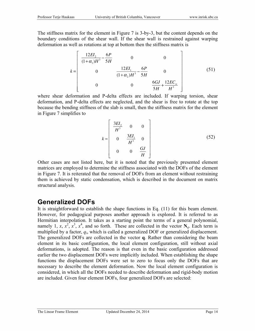
The stiffness matrix for the element in Figure 7 is 3-by-3, but the content depends on the boundary conditions of the shear wall. If the shear wall is restrained against warping deformation as well as rotations at top at bottom then the stiffness matrix is

k =

12EI2(1+α1)H

3 −6P5H

0 0

0 12EI1(1+α 2 )H

3 −6P5H

0

0 0 6GJ5H

+ 12ECw

H 3

⎡

⎣

⎢⎢⎢⎢⎢⎢⎢⎢

⎤

⎦

⎥⎥⎥⎥⎥⎥⎥⎥

(51)

where shear deformation and P-delta effects are included. If warping torsion, shear deformation, and P-delta effects are neglected, and the shear is free to rotate at the top because the bending stiffness of the slab is small, then the stiffness matrix for the element in Figure 7 simplifies to

k =

3EI2H 3 0 0

0 3EI1H 3 0

0 0 GJH

⎡

⎣

⎢⎢⎢⎢⎢⎢⎢

⎤

⎦

⎥⎥⎥⎥⎥⎥⎥

(52)

Other cases are not listed here, but it is noted that the previously presented element matrices are employed to determine the stiffness associated with the DOFs of the element in Figure 7. It is reiterated that the removal of DOFs from an element without restraining them is achieved by static condensation, which is described in the document on matrix structural analysis.

Generalized DOFs It is straightforward to establish the shape functions in Eq. (11) for this beam element. However, for pedagogical purposes another approach is explored. It is referred to as Hermitian interpolation. It takes as a starting point the terms of a general polynomial, namely 1, x, x2, x3, x4, and so forth. These are collected in the vector Nq. Each term is multiplied by a factor, qi, which is called a generalized DOF or generalized displacement. The generalized DOFs are collected in the vector q. Rather than considering the beam element in its basic configuration, the local element configuration, still without axial deformations, is adopted. The reason is that even in the basic configuration addressed earlier the two displacement DOFs were implicitly included. When establishing the shape functions the displacement DOFs were set to zero to focus only the DOFs that are necessary to describe the element deformation. Now the local element configuration is considered, in which all the DOFs needed to describe deformation and rigid-body motion are included. Given four element DOFs, four generalized DOFs are selected:



w(x) = Nqq = 1 x x2 x3{ }q1q2q3q4

⎧

⎨

⎪⎪

⎩

⎪⎪

⎫

⎬

⎪⎪

⎭

⎪⎪

(53)

Next, the generalized DOFs are related to the actual DOFs by the equation u = Aq (54)

In turn, the sought shape functions N in Eq. (14) are obtained by combining Eqs. (53) and (54):

w(x) = Nqq = NqA−1

N

u (55)

The matrix A is established by writing each actual DOF, ui, in terms of the element displacement, w(x):

u1 = w(0) = q1u2 = − ′w (0) = q2u3 = w(L) = q1 + q2L + q3L

2 + q4L3

u4 = − ′w (L) = q2 + q3L + q4L2

(56)

which is summarized in the A-matrix:

u1u2u3u4

⎧

⎨

⎪⎪

⎩

⎪⎪

⎫

⎬

⎪⎪

⎭

⎪⎪

=

1 0 0 00 1 0 01 L L2 L3

0 1 L L2

⎡

⎣

⎢⎢⎢⎢

⎤

⎦

⎥⎥⎥⎥

A

q1q2q3q4

⎧

⎨

⎪⎪

⎩

⎪⎪

⎫

⎬

⎪⎪

⎭

⎪⎪

(57)

Eq. (55) yields the sought shape functions, N = NqA−1 , which substituted into Eq. (14)

produces the stiffness matrix in Eq. (3). This is the same result as any other approach based on polynomial functions for Euler-Bernoulli beams, because for this element the solution to the differential equation is indeed polynomial.

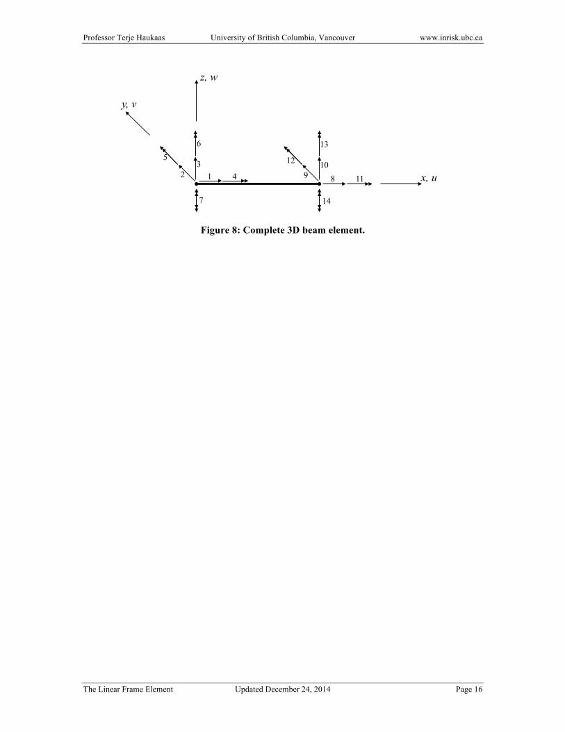
Complete Stiffness Matrix Figure 8 shows the complete 3D element with 7 DOFs per node, including the warping DOFs, number 7 and 14. This is the DOF numbering that is utilized in the structural analysis program St.



Figure 8: Complete 3D beam element.

3 1 2 x, u

z, w

y, v

4

6 5

7

10 8 9 11

13

12

14

Documents

The Linear Frame Element - University of British Columbiainrisk.sites.olt.ubc.ca/files/2012/11/The-Linear-Frame-Element.pdfThe Linear Frame Element Updated December 24, ... body motion