THE LEAST-MEAN-SQUARE (LMS) ALGORITHMscs.etc.tuiasi.ro/iciocoiu/courses/PAS/course/course3/1.pdf · 78 Chapter 3 The Least-Mean-Square (LMS) Algorithm If good estimates of matrix

3THE LEAST-MEAN-SQUARE (LMS)

ALGORITHM

3.1 INTRODUCTION

The least-mean-square (LMS) is a search algorithm in which a simplification of the gradient vectorcomputation is made possible by appropriately modifying the objective function [1]-[2]. The LMSalgorithm, as well as others related to it, is widely used in various applications of adaptive filteringdue to its computational simplicity [3]-[7]. The convergence characteristics of the LMS algorithmare examined in order to establish a range for the convergence factor that will guarantee stability.The convergence speed of the LMS is shown to be dependent on the eigenvalue spread of theinput signal correlation matrix [2]-[6]. In this chapter, several properties of the LMS algorithmare discussed including the misadjustment in stationary and nonstationary environments [2]-[9] andtracking performance [10]-[12]. The analysis results are verified by a large number of simulationexamples. Appendix B, section B.1, complements this chapter by analyzing the finite-wordlengtheffects in LMS algorithms.

The LMS algorithm is by far the most widely used algorithm in adaptive filtering for several reasons.The main features that attracted the use of the LMS algorithm are low computational complexity,proof of convergence in stationary environment, unbiased convergence in the mean to the Wienersolution, and stable behavior when implemented with finite-precision arithmetic. The convergenceanalysis of the LMS presented here utilizes the independence assumption.

3.2 THE LMS ALGORITHM

In Chapter 2 we derived the optimal solution for the parameters of the adaptive filter implementedthrough a linear combiner, which corresponds to the case of multiple input signals. This solution leadsto the minimum mean-square error in estimating the reference signal d(k). The optimal (Wiener)solution is given by

wo = R−1p (3.1)

where R = E[x(k)xT (k)] and p = E[d(k)x(k)], assuming that d(k) and x(k) are jointly wide-sensestationary.

P.S.R. Diniz, Adaptive Filtering, DOI: 10.1007/978-0-387-68606-6_3, © Springer Science+Business Media, LLC 2008

78 Chapter 3 The Least-Mean-Square (LMS) Algorithm

If good estimates of matrix R, denoted by R(k), and of vector p, denoted by p(k), are available,a steepest-descent-based algorithm can be used to search the Wiener solution of equation (3.1) asfollows:

w(k + 1) = w(k)− μgw(k)= w(k) + 2μ(p(k)− R(k)w(k)) (3.2)

for k = 0, 1, 2, . . ., where gw(k) represents an estimate of the gradient vector of the objectivefunction with respect to the filter coefficients.

One possible solution is to estimate the gradient vector by employing instantaneous estimates for Rand p as follows:

R(k) = x(k)xT (k)p(k) = d(k)x(k) (3.3)

The resulting gradient estimate is given by

gw(k) = −2d(k)x(k) + 2x(k)xT (k)w(k)= 2x(k)(−d(k) + xT (k)w(k))= −2e(k)x(k) (3.4)

Note that if the objective function is replaced by the instantaneous square error e2(k), instead of theMSE, the above gradient estimate represents the true gradient vector since

∂e2(k)∂w

=[2e(k)

∂e(k)∂w0(k)

2e(k)∂e(k)∂w1(k)

. . . 2e(k)∂e(k)∂wN (k)

]T= −2e(k)x(k)= gw(k) (3.5)

The resulting gradient-based algorithm is known1 as the least-mean-square (LMS) algorithm, whoseupdating equation is

w(k + 1) = w(k) + 2μe(k)x(k) (3.6)

where the convergence factor μ should be chosen in a range to guarantee convergence.

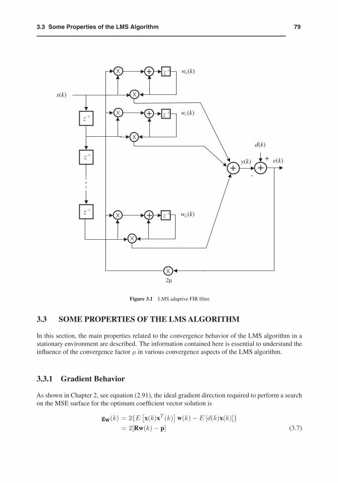
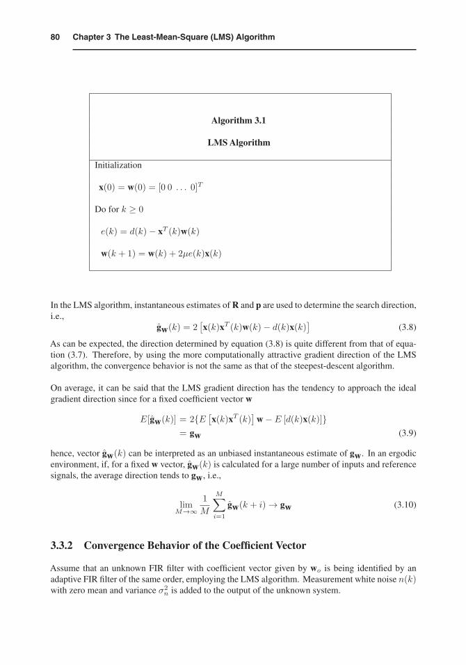
Fig. 3.1 depicts the realization of the LMS algorithm for a delay line input x(k). Typically, oneiteration of the LMS requires N + 2 multiplications for the filter coefficient updating and N + 1multiplications for the error generation. The detailed description of the LMS algorithm is shown inthe table denoted as Algorithm 3.1.

It should be noted that the initialization is not necessarily performed as described in Algorithm 3.1,where the coefficients of the adaptive filter were initialized with zeros. For example, if a roughidea of the optimal coefficient value is known, these values could be used to form w(0) leading to areduction in the number of iterations required to reach the neighborhood of wo.

1Because it minimizes the mean of the squared error.

793.3 Some Properties of the LMS Algorithm

w0 (k)

w1 (k)

wN (k)

+

++-

y(k)

d(k)

x(k)

e(k)

2μ

+

+

+

z -1

z -1

z -1

z -1

z -1z -1

Figure 3.1 LMS adaptive FIR filter.

3.3 SOME PROPERTIES OF THE LMS ALGORITHM

In this section, the main properties related to the convergence behavior of the LMS algorithm in astationary environment are described. The information contained here is essential to understand theinfluence of the convergence factor μ in various convergence aspects of the LMS algorithm.

3.3.1 Gradient Behavior

As shown in Chapter 2, see equation (2.91), the ideal gradient direction required to perform a searchon the MSE surface for the optimum coefficient vector solution is

gw(k) = 2{E [x(k)xT (k)]

w(k)− E [d(k)x(k)]}= 2[Rw(k)− p] (3.7)


Algorithm 3.1

LMS Algorithm

Initialization

x(0) = w(0) = [0 0 . . . 0]T

Do for k ≥ 0

e(k) = d(k)− xT (k)w(k)

w(k + 1) = w(k) + 2μe(k)x(k)

In the LMS algorithm, instantaneous estimates of R and p are used to determine the search direction,i.e.,

gw(k) = 2[x(k)xT (k)w(k)− d(k)x(k)

](3.8)

As can be expected, the direction determined by equation (3.8) is quite different from that of equa-tion (3.7). Therefore, by using the more computationally attractive gradient direction of the LMSalgorithm, the convergence behavior is not the same as that of the steepest-descent algorithm.

On average, it can be said that the LMS gradient direction has the tendency to approach the idealgradient direction since for a fixed coefficient vector w

E[gw(k)] = 2{E [x(k)xT (k)]

w− E [d(k)x(k)]}= gw (3.9)

hence, vector gw(k) can be interpreted as an unbiased instantaneous estimate of gw. In an ergodicenvironment, if, for a fixed w vector, gw(k) is calculated for a large number of inputs and referencesignals, the average direction tends to gw, i.e.,

limM→∞

1M

M∑i=1

gw(k + i)→ gw (3.10)

3.3.2 Convergence Behavior of the Coefficient Vector

Assume that an unknown FIR filter with coefficient vector given by wo is being identified by anadaptive FIR filter of the same order, employing the LMS algorithm. Measurement white noise n(k)with zero mean and variance σ2

n is added to the output of the unknown system.


The error in the adaptive-filter coefficients as related to the ideal coefficient vector wo, in eachiteration, is described by the N + 1-length vector

Δw(k) = w(k)− wo (3.11)

With this definition, the LMS algorithm can alternatively be described by

Δw(k + 1) = Δw(k) + 2μe(k)x(k)= Δw(k) + 2μx(k)

[xT (k)wo + n(k)− xT (k)w(k)

]= Δw(k) + 2μx(k)

[eo(k)− xT (k)Δw(k)

]=[I− 2μx(k)xT (k)

]Δw(k) + 2μeo(k)x(k) (3.12)

where eo(k) is the optimum output error given by

eo(k) = d(k)− wTo x(k)= wTo x(k) + n(k)− wTo x(k)= n(k) (3.13)

The expected error in the coefficient vector is then given by

E[Δw(k + 1)] = E{[I− 2μx(k)xT (k)]Δw(k)}+ 2μE[eo(k)x(k)] (3.14)

If it is assumed that the elements of x(k) are statistically independent of the elements of Δw(k) andeo(k), equation (3.14) can be simplified as follows:

E[Δw(k + 1)] = {I− 2μE[x(k)xT (k)]}E[Δw(k)]= (I− 2μR)E[Δw(k)] (3.15)

The first assumption is justified if we assume that the deviation in the parameters is dependent onprevious input signal vectors only, whereas in the second assumption we also considered that theerror signal at the optimal solution is orthogonal to the elements of the input signal vector. The aboveexpression leads to

E[Δw(k + 1)] = (I− 2μR)k+1E[Δw(0)] (3.16)

Equation (3.15) premultiplied by QT , where Q is the unitary matrix that diagonalizes R through asimilarity transformation, yields

E[QTΔw(k + 1)

]= (I− 2μQTRQ)E

[QTΔw(k)

]= E [Δw′(k + 1)]= (I− 2μΛ)E [Δw′(k)]

=

⎡⎢⎢⎢⎢⎣

1− 2μλ0 0 · · · 0

0 1− 2μλ1...

......

. . ....

0 0 1− 2μλN

⎤⎥⎥⎥⎥⎦E [Δw′(k)]

(3.17)


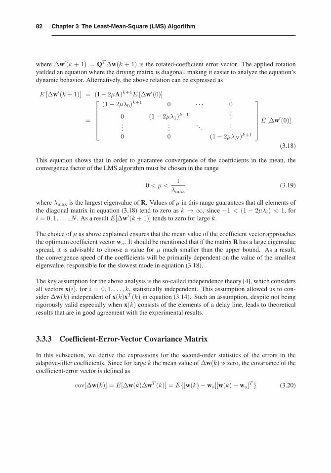
where Δw′(k + 1) = QTΔw(k + 1) is the rotated-coefficient error vector. The applied rotationyielded an equation where the driving matrix is diagonal, making it easier to analyze the equation’sdynamic behavior. Alternatively, the above relation can be expressed as

E [Δw′(k + 1)] = (I− 2μΛ)k+1E [Δw′(0)]

=

⎡⎢⎢⎢⎢⎣

(1− 2μλ0)k+1 0 · · · 0

0 (1− 2μλ1)k+1...

......

. . ....

0 0 (1− 2μλN )k+1

⎤⎥⎥⎥⎥⎦E [Δw′(0)]

(3.18)

This equation shows that in order to guarantee convergence of the coefficients in the mean, theconvergence factor of the LMS algorithm must be chosen in the range

0 < μ <1

λmax(3.19)

where λmax is the largest eigenvalue of R. Values of μ in this range guarantees that all elements ofthe diagonal matrix in equation (3.18) tend to zero as k → ∞, since −1 < (1 − 2μλi) < 1, fori = 0, 1, . . . , N . As a result E[Δw′(k + 1)] tends to zero for large k.

The choice of μ as above explained ensures that the mean value of the coefficient vector approachesthe optimum coefficient vector wo. It should be mentioned that if the matrix R has a large eigenvaluespread, it is advisable to choose a value for μ much smaller than the upper bound. As a result,the convergence speed of the coefficients will be primarily dependent on the value of the smallesteigenvalue, responsible for the slowest mode in equation (3.18).

The key assumption for the above analysis is the so-called independence theory [4], which considersall vectors x(i), for i = 0, 1, . . . , k, statistically independent. This assumption allowed us to con-sider Δw(k) independent of x(k)xT (k) in equation (3.14). Such an assumption, despite not beingrigorously valid especially when x(k) consists of the elements of a delay line, leads to theoreticalresults that are in good agreement with the experimental results.

3.3.3 Coefficient-Error-Vector Covariance Matrix

In this subsection, we derive the expressions for the second-order statistics of the errors in theadaptive-filter coefficients. Since for large k the mean value of Δw(k) is zero, the covariance of thecoefficient-error vector is defined as

cov[Δw(k)] = E[Δw(k)ΔwT (k)] = E{[w(k)− wo][w(k)− wo]T } (3.20)


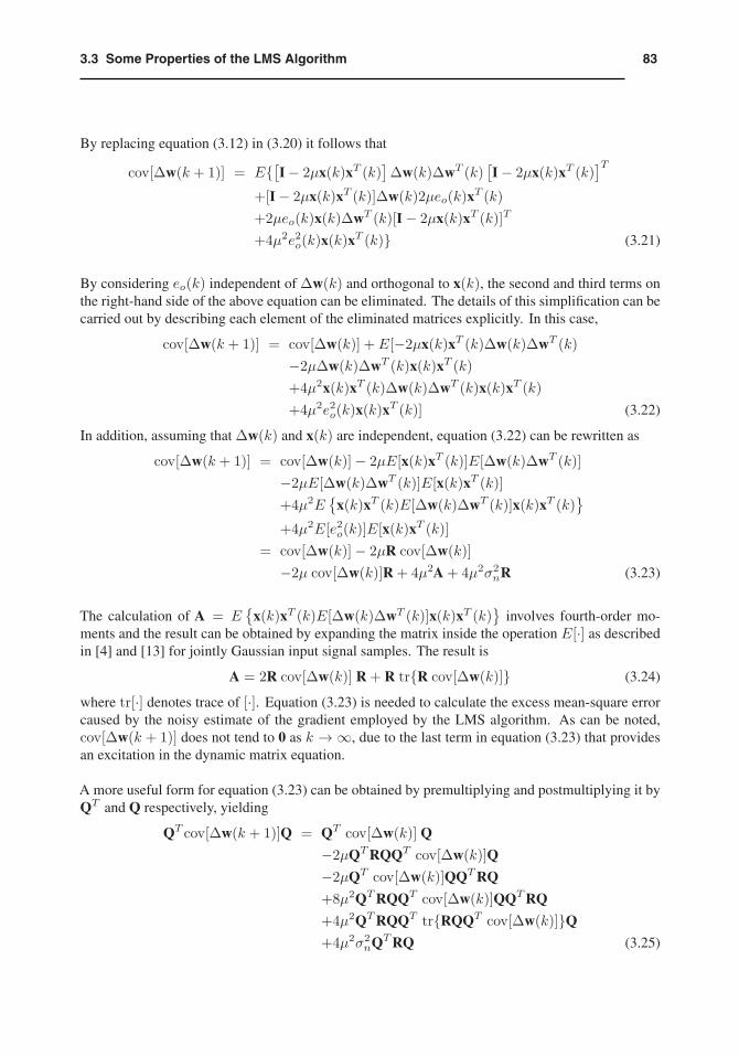
By replacing equation (3.12) in (3.20) it follows that

cov[Δw(k + 1)] = E{[I− 2μx(k)xT (k)]Δw(k)ΔwT (k)

[I− 2μx(k)xT (k)

]T+[I− 2μx(k)xT (k)]Δw(k)2μeo(k)xT (k)+2μeo(k)x(k)ΔwT (k)[I− 2μx(k)xT (k)]T

+4μ2e2o(k)x(k)xT (k)} (3.21)

By considering eo(k) independent of Δw(k) and orthogonal to x(k), the second and third terms onthe right-hand side of the above equation can be eliminated. The details of this simplification can becarried out by describing each element of the eliminated matrices explicitly. In this case,

cov[Δw(k + 1)] = cov[Δw(k)] + E[−2μx(k)xT (k)Δw(k)ΔwT (k)−2μΔw(k)ΔwT (k)x(k)xT (k)+4μ2x(k)xT (k)Δw(k)ΔwT (k)x(k)xT (k)+4μ2e2o(k)x(k)xT (k)] (3.22)

In addition, assuming that Δw(k) and x(k) are independent, equation (3.22) can be rewritten as

cov[Δw(k + 1)] = cov[Δw(k)]− 2μE[x(k)xT (k)]E[Δw(k)ΔwT (k)]−2μE[Δw(k)ΔwT (k)]E[x(k)xT (k)]+4μ2E

{x(k)xT (k)E[Δw(k)ΔwT (k)]x(k)xT (k)

}+4μ2E[e2o(k)]E[x(k)xT (k)]

= cov[Δw(k)]− 2μR cov[Δw(k)]−2μ cov[Δw(k)]R + 4μ2A + 4μ2σ2

nR (3.23)

The calculation of A = E{

x(k)xT (k)E[Δw(k)ΔwT (k)]x(k)xT (k)}

involves fourth-order mo-ments and the result can be obtained by expanding the matrix inside the operation E[·] as describedin [4] and [13] for jointly Gaussian input signal samples. The result is

A = 2R cov[Δw(k)] R + R tr{R cov[Δw(k)]} (3.24)

where tr[·] denotes trace of [·]. Equation (3.23) is needed to calculate the excess mean-square errorcaused by the noisy estimate of the gradient employed by the LMS algorithm. As can be noted,cov[Δw(k + 1)] does not tend to 0 as k → ∞, due to the last term in equation (3.23) that providesan excitation in the dynamic matrix equation.

A more useful form for equation (3.23) can be obtained by premultiplying and postmultiplying it byQT and Q respectively, yielding

QT cov[Δw(k + 1)]Q = QT cov[Δw(k)] Q

−2μQTRQQT cov[Δw(k)]Q−2μQT cov[Δw(k)]QQTRQ

+8μ2QTRQQT cov[Δw(k)]QQTRQ

+4μ2QTRQQT tr{RQQT cov[Δw(k)]}Q+4μ2σ2

nQTRQ (3.25)


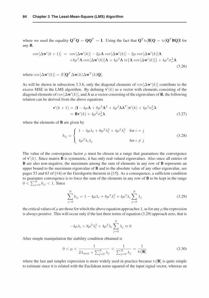
where we used the equality QTQ = QQT = I. Using the fact that QT tr[B]Q = tr[QTBQ]I forany B,

cov[Δw′(k + 1)] = cov[Δw′(k)]− 2μΛ cov[Δw′(k)]− 2μ cov[Δw′(k)]Λ+8μ2Λ cov[Δw′(k)]Λ + 4μ2Λ tr{Λ cov[Δw′(k)]}+ 4μ2σ2

nΛ

(3.26)

where cov[Δw′(k)] = E[QTΔw(k)ΔwT (k)Q].

As will be shown in subsection 3.3.6, only the diagonal elements of cov[Δw′(k)] contribute to theexcess MSE in the LMS algorithm. By defining v′(k) as a vector with elements consisting of thediagonal elements of cov[Δw′(k)], andλ as a vector consisting of the eigenvalues of R, the followingrelation can be derived from the above equations

v′(k + 1) = (I− 4μΛ + 8μ2Λ2 + 4μ2λλT )v′(k) + 4μ2σ2nλ

= Bv′(k) + 4μ2σ2nλ (3.27)

where the elements of B are given by

bij =

⎧⎨⎩

1− 4μλi + 8μ2λ2i + 4μ2λ2

i for i = j

4μ2λiλj for i �= j(3.28)

The value of the convergence factor μ must be chosen in a range that guarantees the convergenceof v′(k). Since matrix B is symmetric, it has only real-valued eigenvalues. Also since all entries ofB are also non-negative, the maximum among the sum of elements in any row of B represents anupper bound to the maximum eigenvalue of B and to the absolute value of any other eigenvalue, seepages 53 and 63 of [14] or the Gershgorin theorem in [15]. As a consequence, a sufficient conditionto guarantee convergence is to force the sum of the elements in any row of B to be kept in the range0 <

∑Nj=0 bij < 1. Since

N∑j=0

bij = 1− 4μλi + 8μ2λ2i + 4μ2λi

N∑j=0

λj (3.29)

the critical values ofμ are those for which the above equation approaches 1, as for anyμ the expressionis always positive. This will occur only if the last three terms of equation (3.29) approach zero, that is

−4μλi + 8μ2λ2i + 4μ2λi

N∑j=0

λj ≈ 0

After simple manipulation the stability condition obtained is

0 < μ <1

2λmax +∑Nj=0 λj

<1∑Nj=0 λj

=1

tr[R](3.30)

where the last and simpler expression is more widely used in practice because tr[R] is quite simpleto estimate since it is related with the Euclidean norm squared of the input signal vector, whereas an


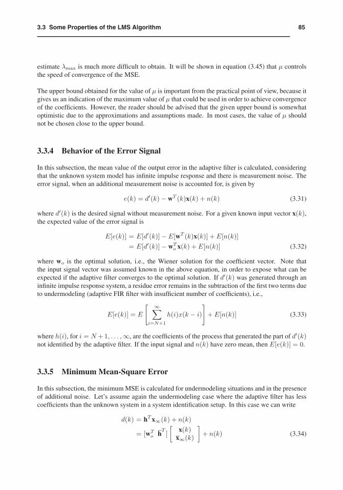
estimate λmax is much more difficult to obtain. It will be shown in equation (3.45) that μ controlsthe speed of convergence of the MSE.

The upper bound obtained for the value of μ is important from the practical point of view, because itgives us an indication of the maximum value of μ that could be used in order to achieve convergenceof the coefficients. However, the reader should be advised that the given upper bound is somewhatoptimistic due to the approximations and assumptions made. In most cases, the value of μ shouldnot be chosen close to the upper bound.

3.3.4 Behavior of the Error Signal

In this subsection, the mean value of the output error in the adaptive filter is calculated, consideringthat the unknown system model has infinite impulse response and there is measurement noise. Theerror signal, when an additional measurement noise is accounted for, is given by

e(k) = d′(k)− wT (k)x(k) + n(k) (3.31)

where d′(k) is the desired signal without measurement noise. For a given known input vector x(k),the expected value of the error signal is

E[e(k)] = E[d′(k)]− E[wT (k)x(k)] + E[n(k)]= E[d′(k)]− wTo x(k) + E[n(k)] (3.32)

where wo is the optimal solution, i.e., the Wiener solution for the coefficient vector. Note thatthe input signal vector was assumed known in the above equation, in order to expose what can beexpected if the adaptive filter converges to the optimal solution. If d′(k) was generated through aninfinite impulse response system, a residue error remains in the subtraction of the first two terms dueto undermodeling (adaptive FIR filter with insufficient number of coefficients), i.e.,

E[e(k)] = E

[ ∞∑i=N+1

h(i)x(k − i)]

+ E[n(k)] (3.33)

where h(i), for i = N +1, . . . ,∞, are the coefficients of the process that generated the part of d′(k)not identified by the adaptive filter. If the input signal and n(k) have zero mean, then E[e(k)] = 0.

3.3.5 Minimum Mean-Square Error

In this subsection, the minimum MSE is calculated for undermodeling situations and in the presenceof additional noise. Let’s assume again the undermodeling case where the adaptive filter has lesscoefficients than the unknown system in a system identification setup. In this case we can write

d(k) = hT x∞(k) + n(k)

= [wTo hT][

x(k)x∞(k)

]+ n(k) (3.34)


where wo is a vector containing the firstN +1 coefficients of the unknown system impulse response,h contains the remaining elements of h. The output signal of an adaptive filter withN+1 coefficientsis given by

y(k) = wT (k)x(k)

In this setup the MSE has the following expression

ξ = E{d2(k)− 2wTo x(k)wT (k)x(k)− 2hT

x∞(k)wT (k)x(k)−2[wT (k)x(k)]n(k) + [wT (k)x(k)]2}

= E

{d2(k)− 2[wT (k) 0T∞]

[x(k)

x∞(k)

][wTo h

T][

x(k)x∞(k)

]−2[wT (k)x(k)]n(k) + [wT (k)x(k)]2

}= E[d2(k)]− 2[wT (k) 0T∞]R∞

[woh

]+ wT (k)Rw(k) (3.35)

where

R∞ = E

{[x(k)

x∞(k)

][xT (k) xT∞(k)]

}and 0∞ is an infinite length vector whose elements are zeros. By calculating the derivative of ξwith respect to the coefficients of the adaptive filter, it follows that (see derivations around equations(2.91) and (2.148))

wo = R−1trunc {p∞}N+1 = R−1trunc{

R∞

[woh

]}N+1

= R−1trunc{R∞h}N+1 (3.36)

where trunc{a}N+1 represents a vector generated by retaining the first N + 1 elements of a. Itshould be noticed that the results of equations (3.35) and (3.36) are algorithm independent.

The minimum mean-square error can be obtained from equation (3.35), when assuming the inputsignal is a white noise uncorrelated with the additional noise signal, that is

ξmin = E[e2(k)]min =∞∑

i=N+1

h2(i)E[x2(k − i)] + E[n2(k)]

=∞∑

i=N+1

h2(i)σ2x + σ2

n (3.37)

This minimum error is achieved when it is assumed that the adaptive-filter multiplier coefficients arefrozen at their optimum values, refer to equation (2.148) for similar discussion. In case the adaptivefilter has sufficient order to model the process that generated d(k), the minimum MSE that can beachieved is equal to the variance of the additional noise, given by σ2

n. The reader should note that theeffect of undermodeling discussed in this subsection generates an excess MSE with respect to σ2

n.


3.3.6 Excess Mean-Square Error and Misadjustment

The result of the previous subsection assumes that the adaptive-filter coefficients converge to theiroptimal values, but in practice this is not so. Although the coefficient vector on average convergesto wo, the instantaneous deviation Δw(k) = w(k) − wo, caused by the noisy gradient estimates,generates an excess MSE. The excess MSE can be quantified as described in the present subsection.The output error at instant k is given by

e(k) = d(k)− wTo x(k)−ΔwT (k)x(k)= eo(k)−ΔwT (k)x(k) (3.38)

thene2(k) = e2o(k)− 2eo(k)ΔwT (k)x(k) + ΔwT (k)x(k)xT (k)Δw(k) (3.39)

The so-called independence theory assumes that the vectors x(k), for all k, are statistically indepen-dent, allowing a simple mathematical treatment for the LMS algorithm. As mentioned before, thisassumption is in general not true, especially in the case where x(k) consists of the elements of a delayline. However, even in this case the use of the independence assumption is justified by the agreementbetween the analytical and the experimental results. With the independence assumption, Δw(k) canbe considered independent of x(k), since only previous input vectors are involved in determiningΔw(k). By using the assumption and applying the expected value operator to equation (3.39), wehave

ξ(k) = E[e2(k)]= ξmin − 2E[ΔwT (k)]E[eo(k)x(k)] + E[ΔwT (k)x(k)xT (k)Δw(k)]= ξmin − 2E[ΔwT (k)]E[eo(k)x(k)] + E{tr[ΔwT (k)x(k)xT (k)Δw(k)]}= ξmin − 2E[ΔwT (k)]E[eo(k)x(k)] + E{tr[x(k)xT (k)Δw(k)ΔwT (k)]} (3.40)

where in the fourth equality we used the property tr[A · B] = tr[B ·A]. The last term of the aboveequation can be rewritten as

tr{E[x(k)xT (k)]E[Δw(k)ΔwT (k)]

}Since R = E[x(k)xT (k)] and by the orthogonality principle E[eo(k)x(k)] = 0, the above equationcan be simplified as follows:

ξ(k) = ξmin + E[ΔwT (k)RΔw(k)] (3.41)

The excess in the MSE is given by

Δξ(k)�= ξ(k)− ξmin = E[ΔwT (k)RΔw(k)]= E{tr[RΔw(k)ΔwT (k)]}= tr{E[RΔw(k)ΔwT (k)]} (3.42)

By using the fact that QQT = I, the following relation results

Δξ(k) = tr{E[QQTRQQTΔw(k)ΔwT (k)QQT ]

}= tr{QΛ cov[Δw′(k)]QT } (3.43)


Therefore,Δξ(k) = tr{Λ cov[Δw′(k)]} (3.44)

From equation (3.27), it is possible to show that

Δξ(k) =N∑i=0

λiv′i(k) = λT v′(k) (3.45)

Since

v′i(k + 1) = (1− 4μλi + 8μ2λ2

i )v′i(k) + 4μ2λi

N∑j=0

λjv′j(k) + 4μ2σ2

nλi (3.46)

and v′i(k + 1) ≈ v′

i(k) for large k, we can apply a summation operation to the above equation inorder to obtain

N∑j=0

λjv′j(k) =

μσ2n

∑Ni=0 λi + 2μ

∑Ni=0 λ

2i v

′i(k)

1− μ∑Ni=0 λi

≈ μσ2n

∑Ni=0 λi

1− μ∑Ni=0 λi

=μσ2

ntr[R]1− μtr[R]

(3.47)

where the term 2μ∑Ni=0 λ

2i v

′i(k) was considered very small as compared to the remaining terms of

the numerator. This assumption is not easily justifiable, but is valid for small values of μ.

The excess mean-square error can then be expressed as

ξexc = limk→∞

Δξ(k) ≈ μσ2ntr[R]

1− μtr[R](3.48)

This equation, for very small μ, can be approximated by

ξexc ≈ μσ2ntr[R] = μ(N + 1)σ2

nσ2x (3.49)

where σ2x is the input signal variance and σ2

n is the additional-noise variance.

The misadjustment M , defined as the ratio between the ξexc and the minimum MSE, is a commonparameter used to compare different adaptive signal processing algorithms. For the LMS algorithm,the misadjustment is given by

M�=ξexc

ξmin≈ μtr[R]

1− μtr[R](3.50)


3.3.7 Transient Behavior

Before the LMS algorithm reaches the steady-state behavior, a number of iterations are spent in thetransient part. During this time, the adaptive-filter coefficients and the output error change from theirinitial values to values close to that of the corresponding optimal solution.

In the case of the adaptive-filter coefficients, the convergence in the mean will follow (N + 1)geometric decaying curves with ratios rwi = (1− 2μλi). Each of these curves can be approximatedby an exponential envelope with time constant τwi as follows (see equation (3.18)) [2]:

rwi = e−1τwi = 1− 1

τwi+

12!τ2

wi

+ · · · (3.51)

where for each iteration, the decay in the exponential envelope is equal to the decay in the originalgeometric curve. In general, rwi is slightly smaller than one, especially for the slowly decreasingmodes corresponding to small λi and μ. Therefore,

rwi = (1− 2μλi) ≈ 1− 1τwi

(3.52)

then

τwi =1

2μλifor i = 0, 1, . . . , N . Note that in order to guarantee convergence of the tap coefficients in the mean,μ must be chosen in the range 0 < μ < 1/λmax (see equation (3.19)).

According to equation (3.30), for the convergence of the MSE the range of values for μ is 0 < μ <1/tr[R], and the corresponding time constant can be calculated from matrix B in equation (3.27), byconsidering the terms in μ2 small as compared to the remaining terms in matrix B. In this case, thegeometric decaying curves have ratios given by rei = (1 − 4μλi) that can be fitted to exponentialenvelopes with time constants given by

τei =1

4μλi(3.53)

for i = 0, 1, . . . , N . In the convergence of both the error and the coefficients, the time required forthe convergence depends on the ratio of eigenvalues of the input signal correlation matrix.

Returning to the tap coefficients case, if μ is chosen to be approximately 1/λmax the correspondingtime constant for the coefficients is given by

τwi ≈ λmax

2λi≤ λmax

2λmin(3.54)

Since the mode with the highest time constant takes longer to reach convergence, the rate of conver-gence is determined by the slowest mode given by τwmax = λmax/(2λmin). Suppose the convergenceis considered achieved when the slowest mode provides an attenuation of 100, i.e.,

e−k

τwmax = 0.01


this requires the following number of iterations in order to reach convergence:

k ≈ 4.6λmax

2λmin

The above situation is quite optimistic because μ was chosen to be high. As mentioned before, inpractice we should choose the value ofμmuch smaller than the upper bound. For an eigenvalue spreadapproximating one, according to equation (3.30) let’s choose μ smaller than 1/[(N + 3)λmax].2 Inthis case, the LMS algorithm will require at least

k ≈ 4.6(N + 3)λmax

2λmin≈ 2.3(N + 3)

iterations to achieve convergence in the coefficients.

The analytical results presented in this section are valid for stationary environments. The LMSalgorithm can also operate in the case of nonstationary environments, as shown in the followingsection.

3.4 LMS ALGORITHM BEHAVIOR IN NONSTATIONARY

ENVIRONMENTS

In practical situations, the environment in which the adaptive filter is embedded may be nonstationary.In these cases, the input signal autocorrelation matrix and/or the cross-correlation vector, denotedrespectively by R(k) and p(k), are/is varying with time. Therefore, the optimal solution for thecoefficient vector is also a time-varying vector given by wo(k).

Since the optimal coefficient vector is not fixed, it is important to analyze if the LMS algorithmwill be able to track changes in wo(k). It is also of interest to learn how the tracking error in thecoefficients given by E[w(k)] − wo(k) will affect the output MSE. It will be shown later that theexcess MSE caused by lag in the tracking of wo(k) can be separated from the excess MSE causedby the measurement noise, and therefore, without loss of generality, in the following analysis theadditional noise will be considered zero.

The coefficient-vector updating in the LMS algorithm can be written in the following form

w(k + 1) = w(k) + 2μx(k)e(k)= w(k) + 2μx(k)[d(k)− xT (k)w(k)] (3.55)

Sinced(k) = xT (k)wo(k) (3.56)

the coefficient updating can be expressed as follows:

w(k + 1) = w(k) + 2μx(k)[xT (k)wo(k)− xT (k)w(k)] (3.57)

2This choice also guarantees the convergence of the MSE.

913.4 LMS Algorithm Behavior in Nonstationary Environments

Now assume that an ensemble of a nonstationary adaptive identification process has been built, wherethe input signal in each experiment is taken from the same stochastic process. The input signal isconsidered stationary. This assumption results in a fixed R matrix, and the nonstationarity is caused bythe desired signal that is generated by applying the input signal to a time-varying system. With theseassumptions, by using the expected value operation to the ensemble, with the coefficient updatingin each experiment given by equation (3.57), and additionally assuming that w(k) is independent ofx(k) yields

E[w(k + 1)] = E[w(k)] + 2μE[x(k)xT (k)]wo(k)− 2μE[x(k)xT (k)]E[w(k)]= E[w(k)] + 2μR{wo(k)− E[w(k)]} (3.58)

If the lag in the coefficient vector is defined by

lw(k) = E[w(k)]− wo(k) (3.59)

equation (3.58) can be rewritten as

lw(k + 1) = (I− 2μR)lw(k)− wo(k + 1) + wo(k) (3.60)

In order to simplify our analysis, we can premultiply the above equation by QT , resulting in adecoupled set of equations given by

l′w(k + 1) = (I− 2μΛ)l′w(k)− w′o(k + 1) + w′

o(k) (3.61)

where the vectors with superscript are the original vectors projected onto the transformed space. Ascan be noted, each element of the lag-error vector is determined by the following relation

l′i(k + 1) = (1− 2μλi)l′i(k)− w′oi(k + 1) + w′

oi(k) (3.62)

where l′i(k) is the ith element of l′w(k). By properly interpreting the above equation, we can say thatthe lag is generated by applying the transformed instantaneous optimal coefficient to a first-orderdiscrete-time lag filter denoted as L

′′i (z), i.e.,

L′i(z) = − z − 1

z − 1 + 2μλiW ′oi(z) = L

′′i (z)W

′oi(z) (3.63)

The discrete-time filter transient response converges with a time constant of the exponential envelopegiven by

τi =1

2μλi(3.64)

which is of course different for each individual tap. Therefore, the tracking ability of the coefficientsin the LMS algorithm is dependent on the eigenvalues of the input signal correlation matrix.

The lag in the adaptive-filter coefficients leads to an excess mean-square error. In order to calculatethe excess MSE, suppose that each element of the optimal coefficient vector is modeled as a first-orderMarkov process. This nonstationary situation can be considered somewhat simplified as comparedwith some real practical situations. However, it allows a manageable mathematical analysis while


retaining the essence of handling the more complicated cases. The first-order Markov process isdescribed by

wo(k) = λwwo(k − 1) + nw(k) (3.65)

where nw(k) is a vector whose elements are zero-mean white noise processes with variance σ2w, and

λw < 1. Note that (1− 2μλi) < λw < 1, for i = 0, 1, . . . , N , since the optimal coefficients valuesmust vary slower than the adaptive-filter tracking speed, i.e., 1

2μλi< 1

1−λw . This model may not

represent an actual system when λw → 1, since the E[wo(k)wTo (k)] will have unbounded elementsif, for example, nw(k) is not exactly zero mean. A more realistic model would include a factor(1 − λw)

p2 , for p ≥ 1, multiplying nw(k) in order to guarantee that E[wo(k)wTo (k)] is bounded.

In the following discussions, this case will not be considered since the corresponding results can beeasily derived (see problem 14).

From equations (3.62) and (3.63), we can infer that the lag-error vector elements are generatedby applying a first-order discrete-time system to the elements of the unknown system coefficientvector, both in the transformed space. On the other hand, the coefficients of the unknown systemare generated by applying each element of the noise vector nw(k) to a first-order all-pole filter,with the pole placed at λw. For the unknown coefficient vector with the above model, the lag-error vector elements can be generated by applying each element of the transformed noise vectorn′

w(k) = QTnw(k) to a discrete-time filter with transfer function

Hi(z) =−(z − 1)z

(z − 1 + 2μλi)(z − λw)(3.66)

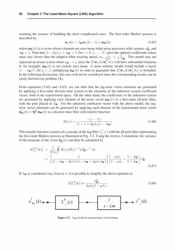
This transfer function consists of a cascade of the lag filter L′′i (z) with the all-pole filter representing

the first-order Markov process as illustrated in Fig. 3.2. Using the inverse Z-transform, the varianceof the elements of the vector l′w(k) can then be calculated by

E[l′2i (k)] =

12πj

∮Hi(z)Hi(z−1)σ2

wz−1 dz

=[

1(1− λw − 2μλi)(1− λw + 2μλiλw)

] [ −μλi1− μλi +

1− λw1 + λw

]σ2

w

(3.67)

If λw is considered very close to 1, it is possible to simplify the above equation as

E[l′2i (k)] ≈ σ2

w4μλi(1− μλi) (3.68)

Figure 3.2 Lag model in nonstationary environment.

933.4 LMS Algorithm Behavior in Nonstationary Environments

Any error in the coefficient vector of the adaptive filter as compared to the optimal coefficient filtergenerates an excess MSE (see equation (3.41)). Since the lag is one source of error in the adaptive-filter coefficients, then the excess MSE due to lag is given by

ξlag = E[lTw(k)Rlw(k)]= E{tr[Rlw(k)lTw(k)]}= tr{RE[lw(k)lTw(k)]}= tr{ΛE[l′w(k)l′Tw (k)]}

=N∑i=0

λiE[l′2i (k)]

≈ σ2w

4μ

N∑i=0

11− μλi (3.69)

If μ is very small, the MSE due to lag tends to infinity indicating that the LMS algorithm, in thiscase, cannot track any change in the environment. On the other hand, for μ appropriately chosenthe algorithm can track variations in the environment leading to an excess MSE. This excess MSEdepends on the variance of the optimal coefficient disturbance and on the values of the input signalautocorrelation matrix eigenvalues, as indicated in equation (3.69). On the other hand, if μ is verysmall and λw is not very close to 1, the approximation for equation (3.67) becomes

E[l′2i (k)] ≈ σ2

w1− λ2

w(3.70)

As a result the MSE due to lag is given by

ξlag ≈ (N + 1)σ2w

1− λ2w

(3.71)

It should be noticed that λw closer to 1 than the modes of the adaptive filter is the common operationregion, therefore the result of equation (3.71) is not discussed further.

Now we analyze how the error due to lag interacts with the error generated by the noisy calculationof the gradient in the LMS algorithm. The overall error in the taps is given by

Δw(k) = w(k)− wo(k) = {w(k)− E[w(k)]}+ {E[w(k)]− wo(k)} (3.72)

where the first error in the above equation is due to the additional noise and the second is the errordue to lag. The overall excess MSE can then be expressed as

ξtotal = E{[w(k)− wo(k)]TR[w(k)− wo(k)]}≈ E{(w(k)− E[w(k)])TR(w(k)− E[w(k)])}

+E{(E[w(k)]− wo(k))TR(E[w(k)]− wo(k))} (3.73)

since 2E{(w(k)−E[w(k)])TR(E[w(k)]−wo(k))} ≈ 0, if we consider the fact that wo(k) is keptfixed in each experiment of the ensemble. As a consequence, an estimate for the overall excess MSE


can be obtained by adding the results of equations (3.48) and (3.69), i.e.,

ξtotal ≈ μσ2ntr[R]

1− μtr[R]+σ2

w4μ

N∑i=0

11− μλi (3.74)

If small μ is employed, the above equation can be simplified as follows:

ξtotal ≈ μσ2ntr[R] +

σ2w

4μ(N + 1) (3.75)

Differentiating the above equation with respect to μ and setting the result to zero yields an optimumvalue for μ given by

μopt =

√(N + 1)σ2

w4σ2

ntr[R](3.76)

The μopt is supposed to lead to the minimum excess MSE. However, the user should bear in mind thatthe μopt can only be used if it satisfies stability conditions, and if its value can be considered smallenough to validate equation (3.75). Also this value is optimum only when quantization effects arenot taken into consideration, where for short-wordlength implementation the best μ should be chosenfollowing the guidelines given in the Appendix B. It should also be mentioned that the study of themisadjustment due to nonstationarity of the environment is considerably more complicated whenthe input signal and the desired signal are simultaneously nonstationary [8], [10]-[17]. Therefore,the analysis presented here is only valid if the assumptions made are valid. However, the simplifiedanalysis provides a good sample of the LMS algorithm behavior in a nonstationary environment andgives a general indication of what can be expected in more complicated situations.

The results of the analysis of the previous sections are obtained assuming that the algorithm is im-plemented with infinite precision3. However, the widespread use of adaptive-filtering algorithms inreal-time requires their implementation with short wordlength, in order to meet the speed require-ments. When implemented with short-wordlength precision the LMS algorithm behavior can be verydifferent from what is expected in infinite precision. In particular, when the convergence factor μtends to zero it is expected that the minimum mean-square error is reached in steady state; however,due to quantization effects the MSE tends to increase significantly if μ is reduced below a certainvalue. In fact, the algorithm can stop updating some filter coefficients ifμ is not chosen appropriately.Appendix B, section B.1, presents detailed analysis of the quantization effects in the LMS algorithm.

3.5 COMPLEX LMS ALGORITHM

The LMS algorithm for complex signals, which often appear in communications applications, isderived in Appendix A. References [18]-[19] provide details related to complex differentiationrequired to generate algorithms working in environments with complex signals.

3This is an abuse of language, by infinite precision we mean very long wordlength.

953.6 Examples

By recalling that the LMS algorithm utilizes instantaneous estimates of matrix R, denoted by R(k),and of vector p, denoted by p(k), given by

R(k) = x(k)xH(k)p(k) = d∗(k)x(k) (3.77)

The actual objective function being minimized is the instantaneous square error |e(k)|2. Accordingto the derivations in section A.3, the expression of the gradient estimate is

gw∗{e(k)e∗(k)} = −e∗(k)x(k) (3.78)

By utilizing the output error definition for the complex environment case and the instantaneousgradient expression, the updating equations for the complex LMS algorithm are described by{

e(k) = d(k)− wH(k)x(k)

w(k + 1) = w(k) + μce∗(k)x(k)

(3.79)

If the convergence factor μc = 2μ, the expressions for the coefficient updating equation of thecomplex and real cases have the same form and the analysis results for the real case equally appliesto the complex case4.

An iteration of the complex LMS requires N + 2 complex multiplications for the filter coefficientupdating and N + 1 complex multiplications for the error generation. In a non-optimized form eachcomplex multiplication requires four real multiplications. The detailed description of the complexLMS algorithm is shown in the table denoted asAlgorithm 3.2. As for any adaptive-filtering algorithm,the initialization is not necessarily performed as described in Algorithm 3.2, where the coefficientsof the adaptive filter are started with zeros.

3.6 EXAMPLES

In this section, a number of examples are presented in order to illustrate the use of the LMS algorithmas well as to verify theoretical results presented in the previous sections.

3.6.1 Analytical Examples

Some analytical tools presented so far are employed to characterize two interesting types of adaptive-filtering problems. The problems are also solved with the LMS algorithm.

Example 3.1

A Gaussian white noise with unit variance colored by a filter with transfer function

4The missing factor 2 here originates from the term 12 in definition of the gradient that we opted to use in order to be

coherent with most literature, in actual implementation the factor 2 of the real case is usually incorporated to the μ.


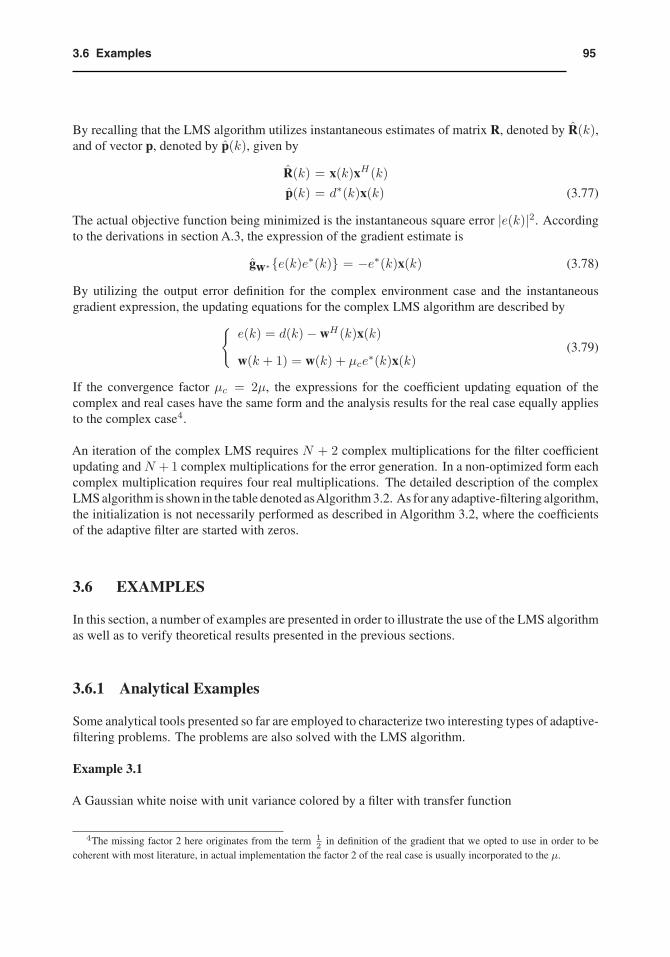
Algorithm 3.2

Complex LMS Algorithm

Initialization

x(0) = w(0) = [0 0 . . . 0]T

Do for k ≥ 0

e(k) = d(k)− wH(k)x(k)

w(k + 1) = w(k) + μce∗(k)x(k)

Hin(z) =1

z − 0.5is transmitted through a communication channel with model given by

Hc(z) =1

z + 0.8

and with the channel noise being Gaussian white noise with variance σ2n = 0.1.

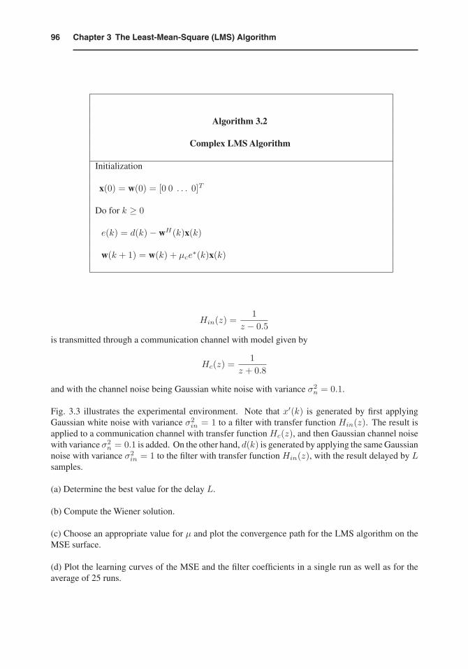
Fig. 3.3 illustrates the experimental environment. Note that x′(k) is generated by first applyingGaussian white noise with variance σ2

in = 1 to a filter with transfer function Hin(z). The result isapplied to a communication channel with transfer function Hc(z), and then Gaussian channel noisewith variance σ2

n = 0.1 is added. On the other hand, d(k) is generated by applying the same Gaussiannoise with variance σ2

in = 1 to the filter with transfer function Hin(z), with the result delayed by Lsamples.

(a) Determine the best value for the delay L.

(b) Compute the Wiener solution.

(c) Choose an appropriate value for μ and plot the convergence path for the LMS algorithm on theMSE surface.

(d) Plot the learning curves of the MSE and the filter coefficients in a single run as well as for theaverage of 25 runs.

973.6 Examples

Solution:

(a) In order to determine L, we will examine the behavior of the cross-correlation between theadaptive-filter input signal denoted by x′(k) and the reference signal d(k).

e(k)y(k)

n(k)

x(k)

d(k)

+-+ Adaptivefilter

HcinH

x (k),

(z) (z)

z -L

Figure 3.3 Channel equalization of Example 3.1.

The cross-correlation between d(k) and x′(k) is given by

p(i) = E[d(k)x′(k − i)]=

12πj

∮Hin(z)z−LziHin(z−1)Hc(z−1)σ2

in

dz

z

=1

2πj

∮1

z − 0.5z−Lzi

z

1− 0.5zz

1 + 0.8zσ2in

dz

z

where the integration path is a counterclockwise closed contour corresponding to the unit circle.

The contour integral of the above equation can be solved through the Cauchy’s residue theorem. ForL = 0 and L = 1, the general solution is

p(0) = E[d(k)x′(k)] = σ2in[0.5

−L+1 10.75

11.4

]

where in order to obtain p(0), we computed the residue at the pole located at 0.5. The values of thecross-correlation for L = 0 and L = 1 are respectively

p(0) = 0.47619p(0) = 0.95238

For L = 2, we have that

p(0) = σ2in[0.5

−L+1 10.75

11.4− 2] = −0.09522

where in this case we computed the residues at the poles located at 0.5 and at 0, respectively. ForL = 3, we have

p(0) = σ2in[

0.5−L+1

1.05− 3.4] = 0.4095


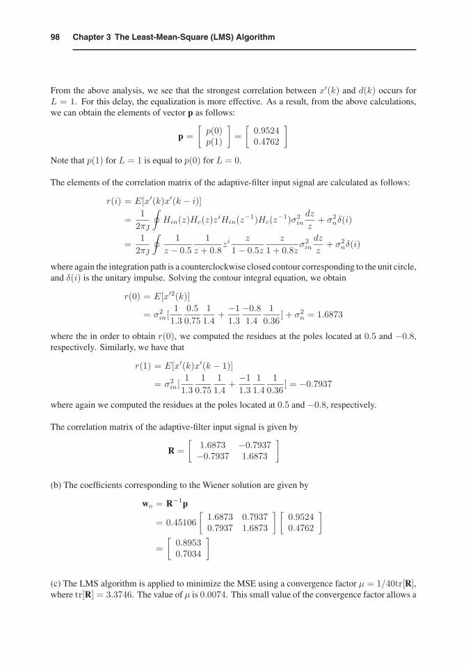
From the above analysis, we see that the strongest correlation between x′(k) and d(k) occurs forL = 1. For this delay, the equalization is more effective. As a result, from the above calculations,we can obtain the elements of vector p as follows:

p =[p(0)p(1)

]=[

0.95240.4762

]Note that p(1) for L = 1 is equal to p(0) for L = 0.

The elements of the correlation matrix of the adaptive-filter input signal are calculated as follows:

r(i) = E[x′(k)x′(k − i)]=

12πj

∮Hin(z)Hc(z)ziHin(z−1)Hc(z−1)σ2

in

dz

z+ σ2

nδ(i)

=1

2πj

∮1

z − 0.51

z + 0.8zi

z

1− 0.5zz

1 + 0.8zσ2in

dz

z+ σ2

nδ(i)

where again the integration path is a counterclockwise closed contour corresponding to the unit circle,and δ(i) is the unitary impulse. Solving the contour integral equation, we obtain

r(0) = E[x′2(k)]

= σ2in[

11.3

0.50.75

11.4

+−11.3−0.81.4

10.36

] + σ2n = 1.6873

where the in order to obtain r(0), we computed the residues at the poles located at 0.5 and −0.8,respectively. Similarly, we have that

r(1) = E[x′(k)x′(k − 1)]

= σ2in[

11.3

10.75

11.4

+−11.3

11.4

10.36

] = −0.7937

where again we computed the residues at the poles located at 0.5 and −0.8, respectively.

The correlation matrix of the adaptive-filter input signal is given by

R =[

1.6873 −0.7937−0.7937 1.6873

]

(b) The coefficients corresponding to the Wiener solution are given by

wo = R−1p

= 0.45106[

1.6873 0.79370.7937 1.6873

] [0.95240.4762

]

=[

0.89530.7034

]

(c) The LMS algorithm is applied to minimize the MSE using a convergence factor μ = 1/40tr[R],where tr[R] = 3.3746. The value of μ is 0.0074. This small value of the convergence factor allows a

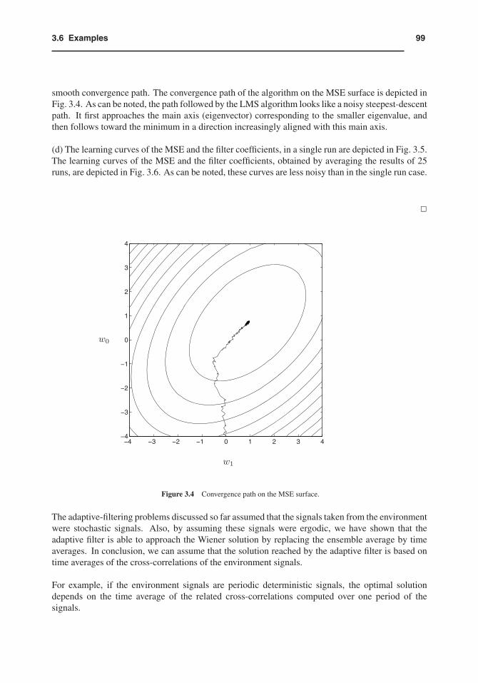
993.6 Examples

smooth convergence path. The convergence path of the algorithm on the MSE surface is depicted inFig. 3.4. As can be noted, the path followed by the LMS algorithm looks like a noisy steepest-descentpath. It first approaches the main axis (eigenvector) corresponding to the smaller eigenvalue, andthen follows toward the minimum in a direction increasingly aligned with this main axis.

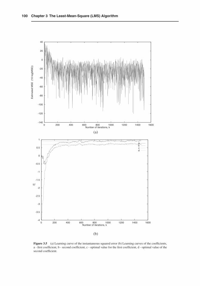
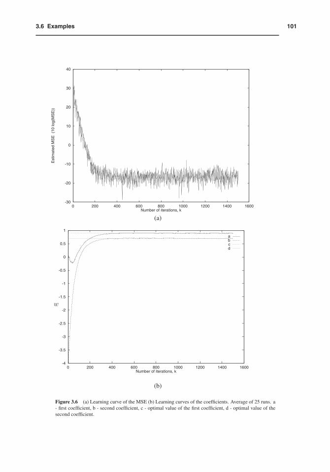
(d) The learning curves of the MSE and the filter coefficients, in a single run are depicted in Fig. 3.5.The learning curves of the MSE and the filter coefficients, obtained by averaging the results of 25runs, are depicted in Fig. 3.6. As can be noted, these curves are less noisy than in the single run case.

�

w0

−4 −3 −2 −1 0 1 2 3 4−4

−3

−2

−1

0

1

2

3

4

w1

Figure 3.4 Convergence path on the MSE surface.

The adaptive-filtering problems discussed so far assumed that the signals taken from the environmentwere stochastic signals. Also, by assuming these signals were ergodic, we have shown that theadaptive filter is able to approach the Wiener solution by replacing the ensemble average by timeaverages. In conclusion, we can assume that the solution reached by the adaptive filter is based ontime averages of the cross-correlations of the environment signals.

For example, if the environment signals are periodic deterministic signals, the optimal solutiondepends on the time average of the related cross-correlations computed over one period of thesignals.


-140

-120

-100

-80

-60

-40

-20

0

20

40

0 200 400 600 800 1000 1200 1400 1600

Est

imat

ed M

SE

(10

log(

MS

E))

Number of iterations, k

(a)

w

-4

-3.5

-3

-2.5

-2

-1.5

-1

-0.5

0

0.5

1

0 200 400 600 800 1000 1200 1400 1600


abcd

(b)

Figure 3.5 (a) Learning curve of the instantaneous squared error (b) Learning curves of the coefficients,a - first coefficient, b - second coefficient, c - optimal value for the first coefficient, d - optimal value of thesecond coefficient.

1013.6 Examples

-30

-20

-10

0

10

20

30

40

0 200 400 600 800 1000 1200 1400 1600

Est

imat

ed M

SE

(10

log(

MS

E))


(a)

w

-4

-3.5

-3

-2.5

-2

-1.5

-1

-0.5

0

0.5

1

0 200 400 600 800 1000 1200 1400 1600


abcd

(b)

Figure 3.6 (a) Learning curve of the MSE (b) Learning curves of the coefficients. Average of 25 runs. a- first coefficient, b - second coefficient, c - optimal value of the first coefficient, d - optimal value of thesecond coefficient.


Note that in this case, the solution obtained using an ensemble average would be time varying sincewe are dealing with a nonstationary problem. The following examples illustrate this issue.

Example 3.2

Suppose in an adaptive-filtering environment, the input signal consists of

x(k) = cos(ω0k)

The desired signal is given byd(k) = sin(ω0k)

where ω0 = 2πM . In this case M = 7.

Compute the optimal solution for a first-order adaptive filter.

Solution:

In this example, the signals involved are deterministic and periodic. If the adaptive-filter coefficientsare fixed, the error is a periodic signal with period M . In this case, the objective function that willbe minimized by the adaptive filter is the average value of the squared error defined by

E[e2(k)] =1M

M−1∑m=0

[e2(k −m)

]= E[d2(k)]− 2wT p + wT Rw (3.80)

where

R =[

E[cos2(ω0k)] E[cos(ω0k) cos(ω0(k − 1))]E[cos(ω0k) cos(ω0(k − 1))] E[cos2(ω0k)]

]

and

p =[E[sin(ω0k) cos(ω0k)] E[sin(ω0k) cos(ω0k − 1)]

]TThe expression for the optimal coefficient vector can be easily derived.

wo = R−1p

Now the above results are applied to the problem described. The elements of the vector p arecalculated as follows:

1033.6 Examples

p =1M

M−1∑m=0

[d(k −m)x(k −m)

d(k −m)x(k −m− 1)

]

=1M

M−1∑m=0

[sin(ω0(k −m)) cos(ω0(k −m))

sin(ω0(k −m)) cos(ω0(k −m− 1))

]

=12

[0

sin(ω0)

]

=[

00.3909

]

The elements of the correlation matrix of the adaptive-filter input signal are calculated as follows:

r(i) = E[x(k)x(k − i)]

=1M

M−1∑m=0

[cos(ω0(k −m)) cos(ω0(k −m− i))]

where

r(0) = E[cos2(ω0(k))] = 0.5r(1) = E[cos(ω0(k)) cos(ω0(k − 1))] = 0.3117

The correlation matrix of the adaptive-filter input signal is given by

R =[

0.5 0.31170.3117 0.5

]

The coefficients corresponding to the optimal solution are given by

wo = R−1p =[ −0.7972

1.2788

]

�

Example 3.3

(a) Assume the input and desired signals are deterministic and periodic with period M . Study theLMS algorithm behavior.

(b) Choose an appropriate value for μ in the previous example and plot the convergence path for theLMS algorithm on the average error surface.


Solution:

(a) It is convenient at this point to recall the coefficient updating of the LMS algorithm

w(k + 1) = w(k) + 2μx(k)e(k) = w(k) + 2μx(k)[d(k)− xT (k)w(k)

]This equation can be rewritten as

w(k + 1) =[I− 2μx(k)xT (k)

]w(k) + 2μd(k)x(k) (3.81)

The solution of equation (3.81), as a function of the initial values of the adaptive-filter coefficients,is given by

w(k + 1) =k∏i=0

[I− 2μx(i)xT (i)

]w(0) +

k∑i=0

⎧⎨⎩

k∏j=i+1

[I− 2μx(j)xT (j)

]2μd(i)x(i)

⎫⎬⎭(3.82)

where we define that∏kj=k+1[·] = 1 for the second product.

Assuming the value of the convergence factor μ is small enough to guarantee that the LMS algorithmwill converge, the first term on the right-hand side of the above equation will vanish as k →∞. Theresulting expression for the coefficient vector is given by

w(k + 1) =k∑i=0

⎧⎨⎩

k∏j=i+1

[I− 2μx(j)xT (j)

]2μd(i)x(i)

⎫⎬⎭

The analysis of the above solution is not straightforward. Following an alternative path based onaveraging the results in a period M , we can reach conclusive results.

Let us define the average value of the adaptive-filter parameters as follows:

w(k + 1) =1M

M−1∑m=0

w(k + 1−m)

Similar definition can be applied to the remaining parameters of the algorithm.

Considering that the signals are deterministic and periodic, we can apply the average operation toequation (3.81). The resulting equation is

w(k + 1) =1M

M−1∑m=0

[I− 2μx(k −m)xT (k −m)

]w(k −m) +

1M

M−1∑m=0

2μd(k −m)x(k −m)

= [I− 2μx(k)xT (k)] w(k) + 2μd(k)x(k) (3.83)

For large k and smallμ, it is expected that the parameters converge to the neighborhood of the optimalsolution. In this case, we can consider that w(k + 1) ≈ w(k) and that the following approximation

1053.6 Examples

is valid

x(k)xT (k)w(k) ≈ x(k)xT (k) w(k)

since the parameters after convergence wander around the optimal solution. Using these approxima-tions in (3.83), the average values of the parameters in the LMS algorithm for periodic signals aregiven by

w(k) ≈ x(k)xT (k)−1d(k)x(k) = R−1p

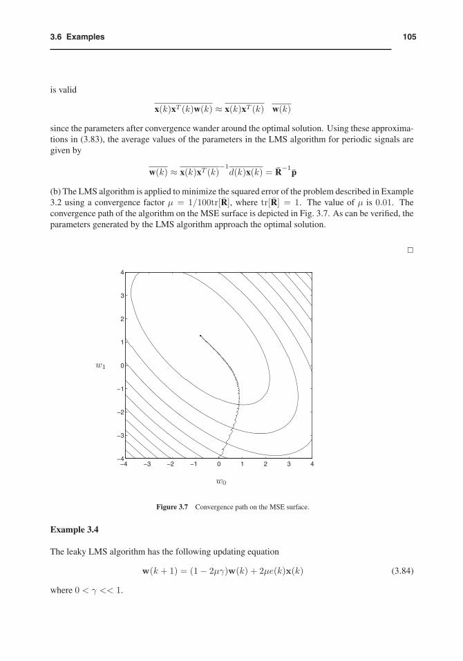
(b) The LMS algorithm is applied to minimize the squared error of the problem described in Example3.2 using a convergence factor μ = 1/100tr[R], where tr[R] = 1. The value of μ is 0.01. Theconvergence path of the algorithm on the MSE surface is depicted in Fig. 3.7. As can be verified, theparameters generated by the LMS algorithm approach the optimal solution.

�

w1

−4 −3 −2 −1 0 1 2 3 4−4

−3

−2

−1

0

1

2

3

4

w0

Figure 3.7 Convergence path on the MSE surface.

Example 3.4

The leaky LMS algorithm has the following updating equation

w(k + 1) = (1− 2μγ)w(k) + 2μe(k)x(k) (3.84)

where 0 < γ << 1.


(a) Compute the range of values of μ such that the coefficients converge in average.

(b) What is the objective function this algorithm actually minimizes?

(c) What happens to the filter coefficients if the error and/or input signals become zero?

Solution:

(a) By utilizing the error expression we generate the coefficient updating equation given by

w(k + 1) = {I− 2μ[x(k)xT (k) + γI]}w(k) + 2μd(k)x(k)

By applying the expectation operation it follows that

E[w(k + 1)] = {I− 2μ[R + γI]}E[w(k)] + 2μp

The inclusion of γ is equivalent to add a white noise to the input signal x(n), such that a value of γis added to the eigenvalues of the input signal autocorrelation matrix. As a result, the condition forthe stability in the mean for the coefficients is expressed as

0 < μ <1

λmax + γ

The coefficients converge to a biased solution with respect to the Wiener solution and are given by

E[w(k)] = [R + γI]−1p

for k →∞.

(b) Equation (3.84) can be rewritten in a form that helps us to recognize the gradient expression.

w(k + 1) = w(k) + 2μ(−γw(k) + e(k)x(k))= w(k)− 2μ(γw(k)− d(k)x(k) + x(k)xT (k)w(k)) (3.85)

By inspection we observe that in this case the gradient is described by

gw(k) = 2γw(k)− 2e(k)x(k) = 2γw(k)− 2d(k)x(k) + 2x(k)xT (k)w(k)

The corresponding objective function that is indeed minimized is given by

ξ(k) = {γ||w(k)||2 + e2(k)}

(c) For zero input or zero error signal after some initial iterations, the dynamic updating equation(3.84) has zero excitation. Since the eigenvalues of the transition matrix {I− 2μ[x(k)xT (k) + γI]}are smaller than one, then the adaptive-filter coefficients will tend to zero for large k.

�

1073.6 Examples

3.6.2 System Identification Simulations

In this subsection, a system identification problem is described and solved by using the LMS algo-rithm. In the following chapters the same problem will be solved using other algorithms presentedin the book. For the FIR adaptive filters the following identification problem is posed:

Example 3.5

An adaptive-filtering algorithm is used to identify a system with impulse response given below.

h = [0.1 0.3 0.0 − 0.2 − 0.4 − 0.7 − 0.4 − 0.2]T

Consider three cases for the input signal: colored noises with variance σ2x = 1 and eigenvalue spread

of their correlation matrix equal to 1.0, 20, and 80, respectively. The measurement noise is Gaussianwhite noise uncorrelated with the input and with variance σ2

n = 10−4. The adaptive filter has 8coefficients.

(a) Run the algorithm and comment on the convergence behavior in each case.

(b) Measure the misadjustment in each example and compare with the theoretical results where ap-propriate.

(c) Considering that fixed-point arithmetic is used, run the algorithm for a set of experiments andcalculate the expected values for ||Δw(k)Q||2 and ξ(k)Q for the following case:

Additional noise: white noise with variance σ2n = 0.0015

Coefficient wordlength: bc = 16 bitsSignal wordlength: bd = 16 bitsInput signal: Gaussian white noise with variance σ2

x = 1.0

(d) Repeat the previous experiment for the following casesbc = 12 bits, bd = 12 bits.bc = 10 bits, bd = 10 bits.

(e) Suppose the unknown system is a time-varying system whose coefficients are first-order Markovprocesses with λw = 0.99 and σ2

w = 0.0015. The initial time-varying-system multiplier coefficientsare the ones above described. The input signal is Gaussian white noise with variance σ2

x = 1.0, andthe measurement noise is also Gaussian white noise independent of the input signal and of theelements of nw(k), with variance σ2

n = 0.01. Simulate the experiment described, measure the totalexcess MSE, and compare to the calculated results.


Solution:

(a) The colored input signal is generated by applying Gaussian white noise, with variance σ2v , to a

first-order filter with transfer function

H(z) =z

z − aAs can be shown from the equation (2.83), the input signal correlation matrix in this case is given by

R =σ2v

1− a2

⎡⎢⎢⎢⎣

1 a · · · a7

a 1 · · · a6

......

. . ....

a7 a6 · · · 1

⎤⎥⎥⎥⎦

The proper choice of the value of a, in order to obtain the desired eigenvalue spread, is not astraightforward task. Some guidelines are now discussed. For example, if the adaptive filter is offirst order, the matrix R is two by two with eigenvalues

λmax =σ2v

1− a2 (1 + a)

and

λmin =σ2v

1− a2 (1− a)

respectively. In this case, the choice of a is straightforward.

In general, it can be shown that

λmax

λmin≤ |Hmax(ejω)|2|Hmin(ejω)|2

For a very large order adaptive filter, the eigenvalue spread approaches

λmax

λmin≈ |Hmax(ejω)|2|Hmin(ejω)|2 =

{1 + a

1− a}2

where the details to reach this result can be found in page 124 of [20].

Using the above relations as guidelines, we reached the correct values of a. These values area = 0.6894 and a = 0.8702 for eigenvalue spreads of 20 and 80, respectively.

Since the variance of the input signal should be unity, the variance of the Gaussian white noise thatproduces x(k) should be given by

σ2v = 1− a2

1093.6 Examples

For the LMS algorithm, we first calculate the upper bound for μ (μmax) to guarantee the algorithmstability, and run the algorithm for μmax, μmax/5, and μmax/10.

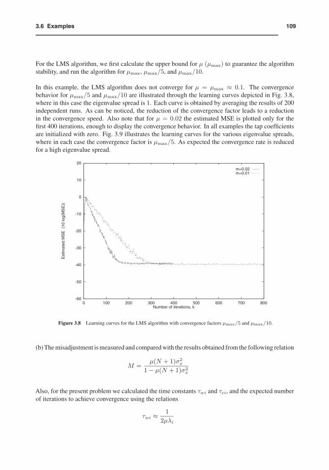
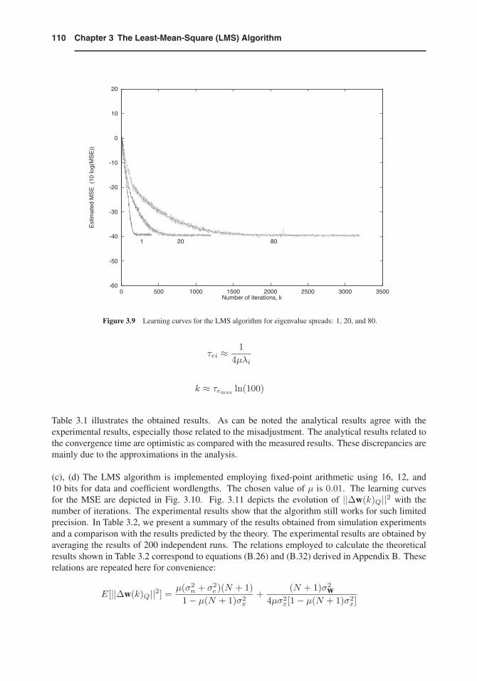
In this example, the LMS algorithm does not converge for μ = μmax ≈ 0.1. The convergencebehavior for μmax/5 and μmax/10 are illustrated through the learning curves depicted in Fig. 3.8,where in this case the eigenvalue spread is 1. Each curve is obtained by averaging the results of 200independent runs. As can be noticed, the reduction of the convergence factor leads to a reductionin the convergence speed. Also note that for μ = 0.02 the estimated MSE is plotted only for thefirst 400 iterations, enough to display the convergence behavior. In all examples the tap coefficientsare initialized with zero. Fig. 3.9 illustrates the learning curves for the various eigenvalue spreads,where in each case the convergence factor is μmax/5. As expected the convergence rate is reducedfor a high eigenvalue spread.

-60

-50

-40

-30

-20

-10

0

10

20

0 100 200 300 400 500 600 700 800

Est

imat

ed M

SE

(10

log(

MS

E))


m=0.02m=0.01

Figure 3.8 Learning curves for the LMS algorithm with convergence factors μmax/5 and μmax/10.

(b) The misadjustment is measured and compared with the results obtained from the following relation

M =μ(N + 1)σ2

x

1− μ(N + 1)σ2x

Also, for the present problem we calculated the time constants τwi and τei, and the expected numberof iterations to achieve convergence using the relations

τwi ≈ 12μλi


-60

-50

-40

-30

-20

-10

0

10

20

0 500 1000 1500 2000 2500 3000 3500

Est

imat

ed M

SE

(10

log(

MS

E))


1 20 80

Figure 3.9 Learning curves for the LMS algorithm for eigenvalue spreads: 1, 20, and 80.

τei ≈ 14μλi

k ≈ τemax ln(100)

Table 3.1 illustrates the obtained results. As can be noted the analytical results agree with theexperimental results, especially those related to the misadjustment. The analytical results related tothe convergence time are optimistic as compared with the measured results. These discrepancies aremainly due to the approximations in the analysis.

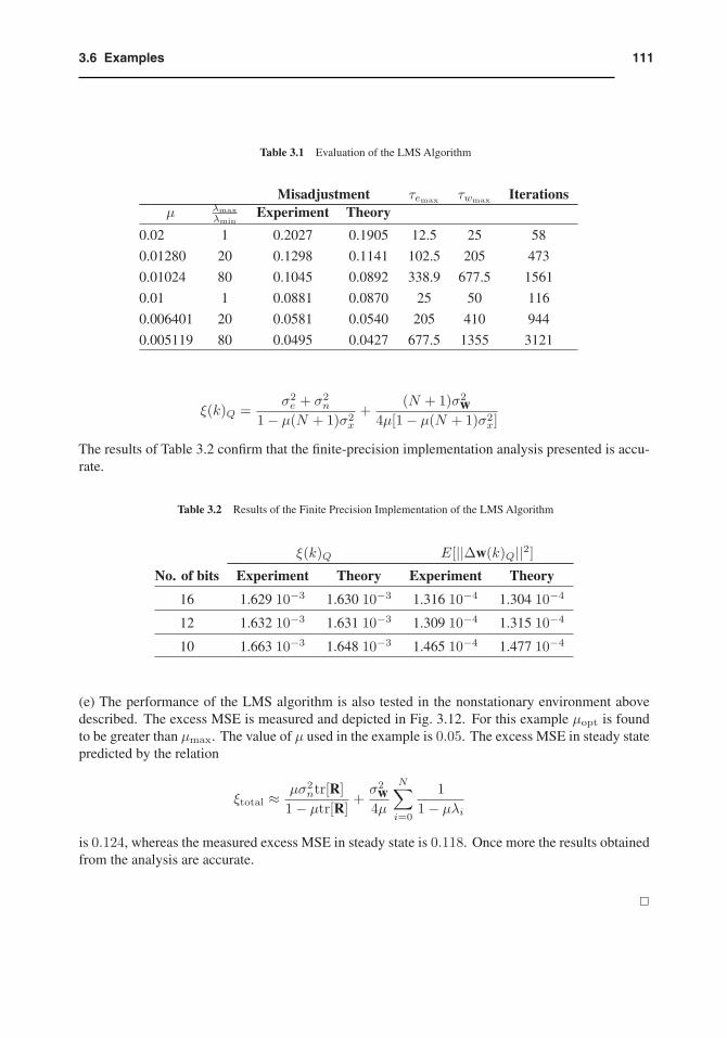
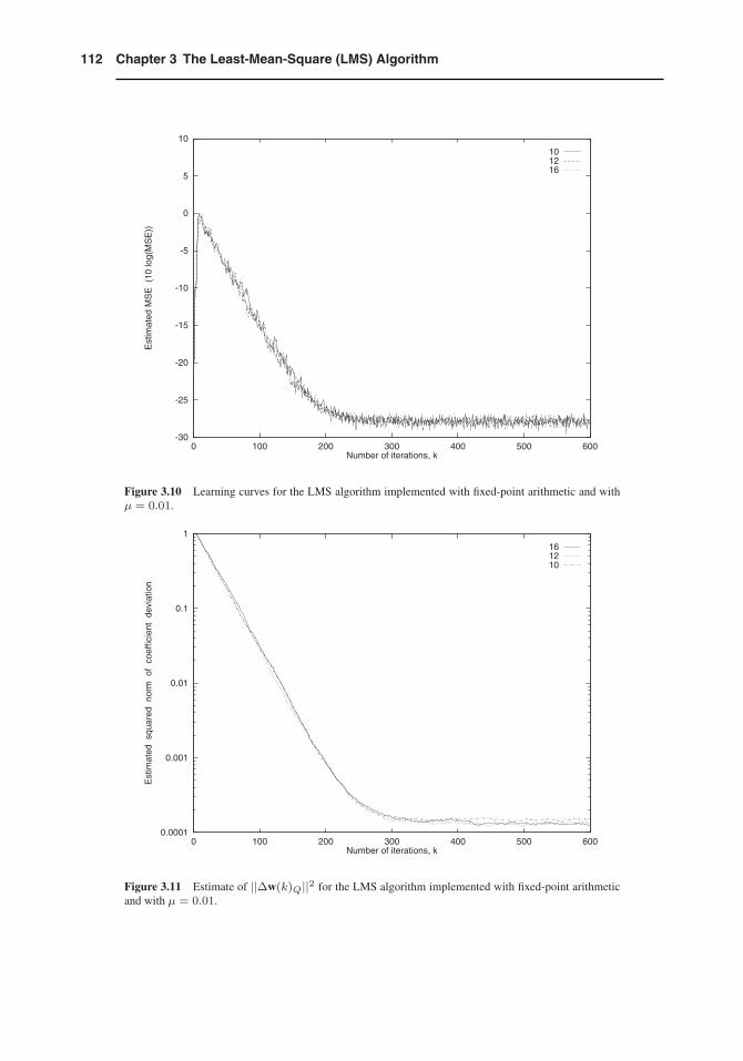
(c), (d) The LMS algorithm is implemented employing fixed-point arithmetic using 16, 12, and10 bits for data and coefficient wordlengths. The chosen value of μ is 0.01. The learning curvesfor the MSE are depicted in Fig. 3.10. Fig. 3.11 depicts the evolution of ||Δw(k)Q||2 with thenumber of iterations. The experimental results show that the algorithm still works for such limitedprecision. In Table 3.2, we present a summary of the results obtained from simulation experimentsand a comparison with the results predicted by the theory. The experimental results are obtained byaveraging the results of 200 independent runs. The relations employed to calculate the theoreticalresults shown in Table 3.2 correspond to equations (B.26) and (B.32) derived in Appendix B. Theserelations are repeated here for convenience:

E[||Δw(k)Q||2] =μ(σ2

n + σ2e)(N + 1)

1− μ(N + 1)σ2x

+(N + 1)σ2

w4μσ2

x[1− μ(N + 1)σ2x]

1113.6 Examples

Table 3.1 Evaluation of the LMS Algorithm

Misadjustment τemax τwmax Iterationsμ λmax

λminExperiment Theory

0.02 1 0.2027 0.1905 12.5 25 58

0.01280 20 0.1298 0.1141 102.5 205 473

0.01024 80 0.1045 0.0892 338.9 677.5 1561

0.01 1 0.0881 0.0870 25 50 116

0.006401 20 0.0581 0.0540 205 410 944

0.005119 80 0.0495 0.0427 677.5 1355 3121

ξ(k)Q =σ2e + σ2

n

1− μ(N + 1)σ2x

+(N + 1)σ2

w4μ[1− μ(N + 1)σ2

x]

The results of Table 3.2 confirm that the finite-precision implementation analysis presented is accu-rate.

Table 3.2 Results of the Finite Precision Implementation of the LMS Algorithm

ξ(k)Q E[||Δw(k)Q||2]No. of bits Experiment Theory Experiment Theory

16 1.629 10−3 1.630 10−3 1.316 10−4 1.304 10−4

12 1.632 10−3 1.631 10−3 1.309 10−4 1.315 10−4

10 1.663 10−3 1.648 10−3 1.465 10−4 1.477 10−4

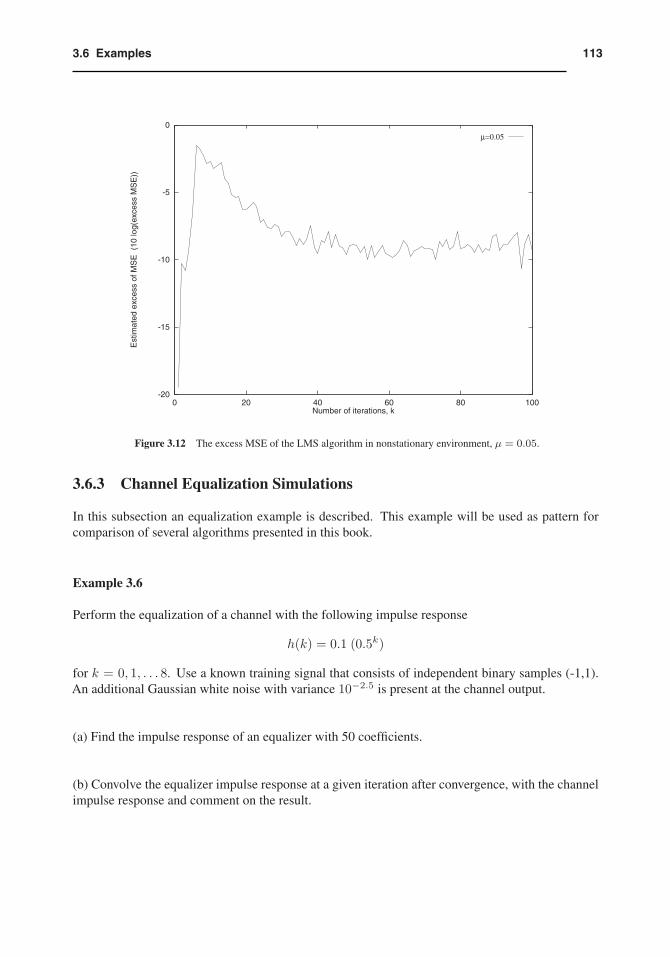
(e) The performance of the LMS algorithm is also tested in the nonstationary environment abovedescribed. The excess MSE is measured and depicted in Fig. 3.12. For this example μopt is foundto be greater than μmax. The value of μ used in the example is 0.05. The excess MSE in steady statepredicted by the relation

ξtotal ≈ μσ2ntr[R]

1− μtr[R]+σ2

w4μ

N∑i=0

11− μλi

is 0.124, whereas the measured excess MSE in steady state is 0.118. Once more the results obtainedfrom the analysis are accurate.

�


-30

-25

-20

-15

-10

-5

0

5

10

0 100 200 300 400 500 600

Est

imat

ed M

SE

(10

log(

MS

E))


101216

Figure 3.10 Learning curves for the LMS algorithm implemented with fixed-point arithmetic and withμ = 0.01.

0.0001

0.001

0.01

0.1

1

0 100 200 300 400 500 600

Est

imat

ed s

quar

ed n

orm

of

coef

ficie

nt d

evia

tion


161210

Figure 3.11 Estimate of ||Δw(k)Q||2 for the LMS algorithm implemented with fixed-point arithmeticand with μ = 0.01.

1133.6 Examples

-20

-15

-10

-5

0

0 20 40 60 80 100

Est

imat

ed e

xces

s of

MS

E (

10 lo

g(ex

cess

MS

E))


μ=0.05

Figure 3.12 The excess MSE of the LMS algorithm in nonstationary environment, μ = 0.05.

3.6.3 Channel Equalization Simulations

In this subsection an equalization example is described. This example will be used as pattern forcomparison of several algorithms presented in this book.

Example 3.6

Perform the equalization of a channel with the following impulse response

h(k) = 0.1 (0.5k)

for k = 0, 1, . . . 8. Use a known training signal that consists of independent binary samples (-1,1).An additional Gaussian white noise with variance 10−2.5 is present at the channel output.

(a) Find the impulse response of an equalizer with 50 coefficients.

(b) Convolve the equalizer impulse response at a given iteration after convergence, with the channelimpulse response and comment on the result.


Solution:

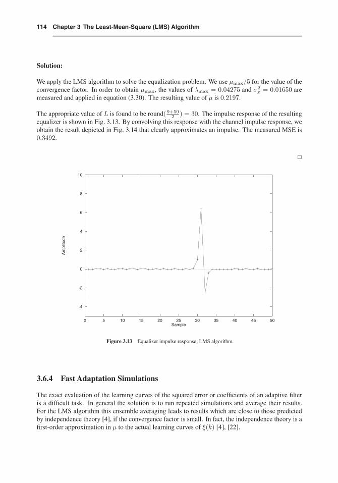
We apply the LMS algorithm to solve the equalization problem. We use μmax/5 for the value of theconvergence factor. In order to obtain μmax, the values of λmax = 0.04275 and σ2

x = 0.01650 aremeasured and applied in equation (3.30). The resulting value of μ is 0.2197.

The appropriate value of L is found to be round( 9+502 ) = 30. The impulse response of the resulting

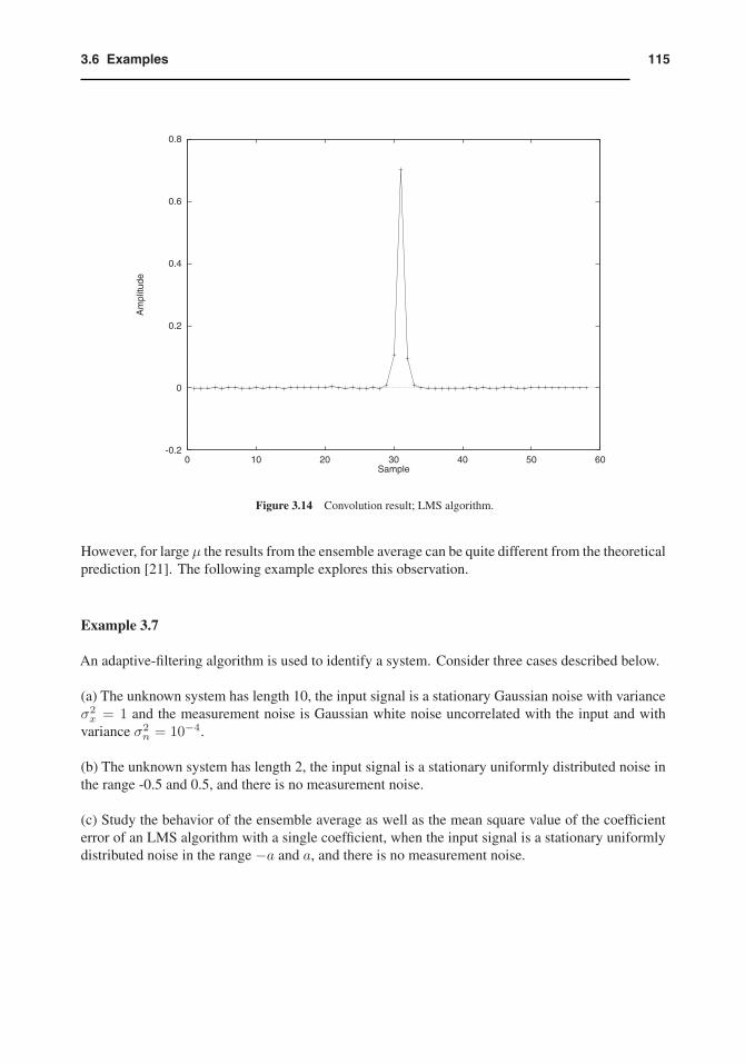
equalizer is shown in Fig. 3.13. By convolving this response with the channel impulse response, weobtain the result depicted in Fig. 3.14 that clearly approximates an impulse. The measured MSE is0.3492.

�

-4

-2

0

2

4

6

8

10

0 5 10 15 20 25 30 35 40 45 50

Am

plitu

de

Sample

Figure 3.13 Equalizer impulse response; LMS algorithm.

3.6.4 Fast Adaptation Simulations

The exact evaluation of the learning curves of the squared error or coefficients of an adaptive filteris a difficult task. In general the solution is to run repeated simulations and average their results.For the LMS algorithm this ensemble averaging leads to results which are close to those predictedby independence theory [4], if the convergence factor is small. In fact, the independence theory is afirst-order approximation in μ to the actual learning curves of ξ(k) [4], [22].

1153.6 Examples

-0.2

0

0.2

0.4

0.6

0.8

0 10 20 30 40 50 60

Am

plitu

de

Sample

Figure 3.14 Convolution result; LMS algorithm.

However, for large μ the results from the ensemble average can be quite different from the theoreticalprediction [21]. The following example explores this observation.

Example 3.7

An adaptive-filtering algorithm is used to identify a system. Consider three cases described below.

(a) The unknown system has length 10, the input signal is a stationary Gaussian noise with varianceσ2x = 1 and the measurement noise is Gaussian white noise uncorrelated with the input and with

variance σ2n = 10−4.

(b) The unknown system has length 2, the input signal is a stationary uniformly distributed noise inthe range -0.5 and 0.5, and there is no measurement noise.

(c) Study the behavior of the ensemble average as well as the mean square value of the coefficienterror of an LMS algorithm with a single coefficient, when the input signal is a stationary uniformlydistributed noise in the range −a and a, and there is no measurement noise.


Solution:

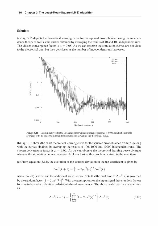
(a) Fig. 3.15 depicts the theoretical learning curve for the squared error obtained using the indepen-dence theory as well as the curves obtained by averaging the results of 10 and 100 independent runs.The chosen convergence factor is μ = 0.08. As we can observe the simulation curves are not closeto the theoretical one, but they get closer as the number of independent runs increases.

0.0001

0.001

0.01

0.1

1

10

0 200 400 600 800 1000

MSE

(L

og s

cale

)


10 runs100 runs

theory

Figure 3.15 Learning curves for the LMS algorithm with convergence factorμ = 0.08, result of ensembleaverages with 10 and 100 independent simulations as well as the theoretical curve.

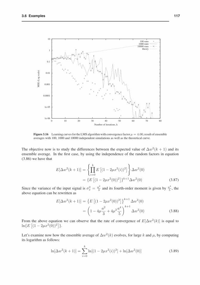
(b) Fig. 3.16 shows the exact theoretical learning curve for the squared error obtained from [23] alongwith the curves obtained by averaging the results of 100, 1000 and 10000 independent runs. Thechosen convergence factor is μ = 4.00. As we can observe the theoretical learning curve divergeswhereas the simulation curves converge. A closer look at this problem is given in the next item.

(c) From equation (3.12), the evolution of the squared deviation in the tap coefficient is given by

Δw2(k + 1) =[1− 2μx2(k)

]2Δw2(k)

where Δw(0) is fixed, and the additional noise is zero. Note that the evolution of Δw2(k) is governed

by the random factor[1− 2μx2(k)

]2. With the assumptions on the input signal these random factors

form an independent, identically distributed random sequence. The above model can then be rewrittenas

Δw2(k + 1) =

{k∏i=0

[1− 2μx2(i)

]2}Δw2(0) (3.86)

1173.6 Examples

1e-06

1e-05

0.0001

0.001

0.01

0.1

1

10

0 10 20 30 40 50 60 70 80

MSE

(L

og s

cale

)


100 runs1000 runs

10000 runstheory

Figure 3.16 Learning curves for the LMS algorithm with convergence factorμ = 4.00, result of ensembleaverages with 100, 1000 and 10000 independent simulations as well as the theoretical curve.

The objective now is to study the differences between the expected value of Δw2(k + 1) and itsensemble average. In the first case, by using the independence of the random factors in equation(3.86) we have that

E[Δw2(k + 1)] =

{k∏i=0

E[(1− 2μx2(i))2

]}Δw2(0)

= {E [(1− 2μx2(0))2]}k+1Δw2(0) (3.87)

Since the variance of the input signal is σ2x = a2

3 and its fourth-order moment is given by a4

5 , theabove equation can be rewritten as

E[Δw2(k + 1)] ={E[(1− 2μx2(0))2

]}k+1Δw2(0)

=(

1− 4μa2

3+ 4μ2 a

4

5

)k+1

Δw2(0) (3.88)

From the above equation we can observe that the rate of convergence of E[Δw2(k)] is equal toln{E [(1− 2μx2(0))2

]}.Let’s examine now how the ensemble average of Δw2(k) evolves, for large k and μ, by computingits logarithm as follows:

ln[Δw2(k + 1)] =k∑i=0

ln[(1− 2μx2(i))2] + ln[Δw2(0)] (3.89)


By assuming that ln[(1 − 2μx2(i))2] exists and by employing the law of large numbers [13], weobtain

ln[Δw2(k + 1)]k + 1

=1

k + 1

{k∑i=0

ln[(1− 2μx2(i))2] + ln[Δw2(0)]

}(3.90)

which converges asymptotically to

E{ln[(1− 2μx2(i))2]}For large k, after some details found in [21], from the above relation it can be concluded that

Δw2(k + 1) ≈ Ce(k+1)E{ln[(1−2μx2(i))2]} (3.91)

whereC is a positive number which is not a constant and will be different for each run of the algorithm.In fact, C can have quite large values for some particular runs. In conclusion, the ensemble averageof Δw2(k+ 1) decreases or increases with a time constant close to E{ln[(1− 2μx2(i))2]}−1. Alsoit converges to zero if and only if E{ln[(1 − 2μx2(i))2]} < 0, leading to a distinct convergencecondition on 2μx2(i) from that obtained by the mean-square stability. In fact, there is a range ofvalues of the convergence factor in which the ensemble average converges but the mean-square valuediverges, explaining the convergence behavior in Fig. 3.16.

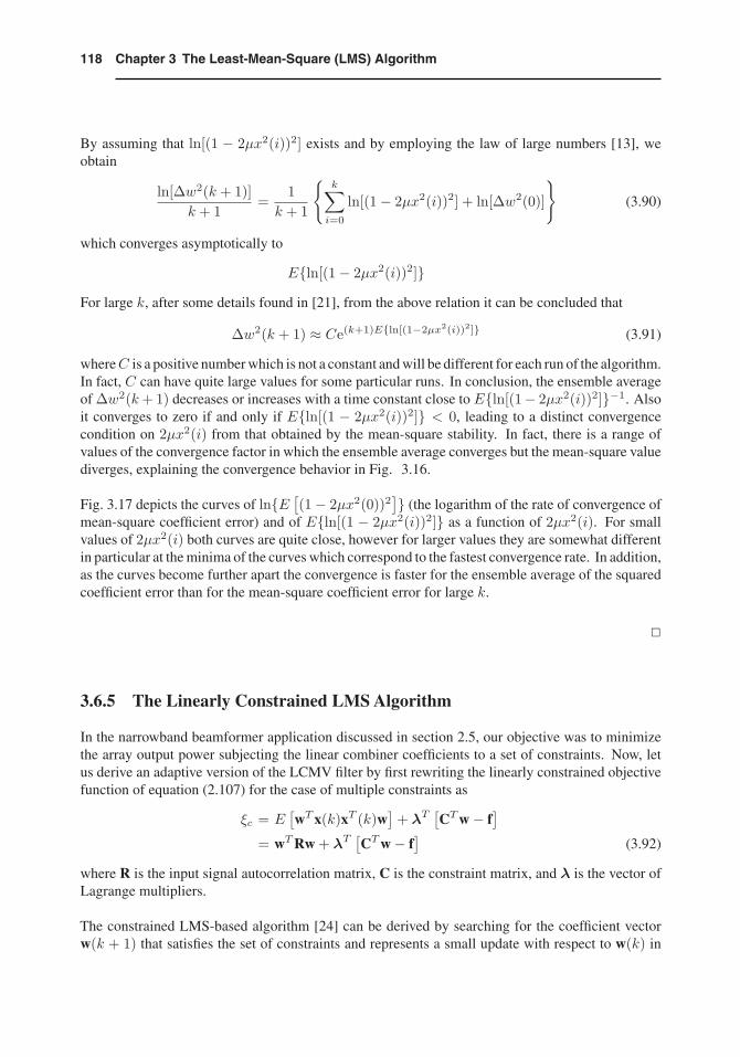
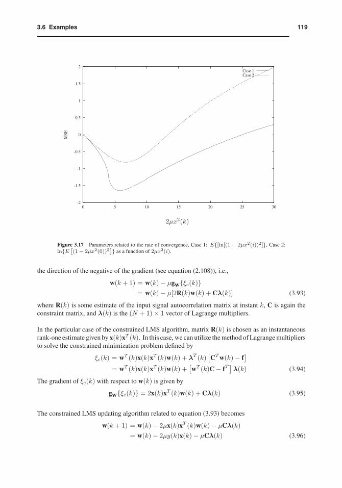
Fig. 3.17 depicts the curves of ln{E [(1− 2μx2(0))2]} (the logarithm of the rate of convergence of

mean-square coefficient error) and of E{ln[(1 − 2μx2(i))2]} as a function of 2μx2(i). For smallvalues of 2μx2(i) both curves are quite close, however for larger values they are somewhat differentin particular at the minima of the curves which correspond to the fastest convergence rate. In addition,as the curves become further apart the convergence is faster for the ensemble average of the squaredcoefficient error than for the mean-square coefficient error for large k.

�

3.6.5 The Linearly Constrained LMS Algorithm

In the narrowband beamformer application discussed in section 2.5, our objective was to minimizethe array output power subjecting the linear combiner coefficients to a set of constraints. Now, letus derive an adaptive version of the LCMV filter by first rewriting the linearly constrained objectivefunction of equation (2.107) for the case of multiple constraints as

ξc = E[wT x(k)xT (k)w

]+ λT

[CTw− f

]= wTRw + λT

[CTw− f

](3.92)

where R is the input signal autocorrelation matrix, C is the constraint matrix, and λ is the vector ofLagrange multipliers.

The constrained LMS-based algorithm [24] can be derived by searching for the coefficient vectorw(k + 1) that satisfies the set of constraints and represents a small update with respect to w(k) in

1193.6 Examples

-2

-1.5

-1

-0.5

0

0.5

1

1.5

2

0 5 10 15 20 25 30

MSE

Case 1Case 2

2μx2(k)

Figure 3.17 Parameters related to the rate of convergence, Case 1: E{[ln[(1 − 2μx2(i))2]}, Case 2:ln{E [

(1 − 2μx2(0))2]} as a function of 2μx2(i).

the direction of the negative of the gradient (see equation (2.108)), i.e.,

w(k + 1) = w(k)− μgw{ξc(k)}= w(k)− μ[2R(k)w(k) + Cλ(k)] (3.93)

where R(k) is some estimate of the input signal autocorrelation matrix at instant k, C is again theconstraint matrix, and λ(k) is the (N + 1)× 1 vector of Lagrange multipliers.

In the particular case of the constrained LMS algorithm, matrix R(k) is chosen as an instantaneousrank-one estimate given by x(k)xT (k). In this case, we can utilize the method of Lagrange multipliersto solve the constrained minimization problem defined by

ξc(k) = wT (k)x(k)xT (k)w(k) + λT (k)[CTw(k)− f

]= wT (k)x(k)xT (k)w(k) +

[wT (k)C− fT

]λ(k) (3.94)

The gradient of ξc(k) with respect to w(k) is given by

gw{ξc(k)} = 2x(k)xT (k)w(k) + Cλ(k) (3.95)

The constrained LMS updating algorithm related to equation (3.93) becomes

w(k + 1) = w(k)− 2μx(k)xT (k)w(k)− μCλ(k)= w(k)− 2μy(k)x(k)− μCλ(k) (3.96)


If we apply the constraint relation CTw(k + 1) = f to the above expression, it follows that

CTw(k + 1) = f

= CTw(k)− 2μCT x(k)xT (k)w(k)− μCTCλ(k)= CTw(k)− 2μy(k)CT x(k)− μCTCλ(k) (3.97)

By solving the above equation for μλ(k) we get

μλ(k) =[CTC

]−1CT [w(k)− 2μy(k)x(k)]− [CTC

]−1f (3.98)

If we substitute equation (3.98) in the updating equation (3.96), we obtain

w(k + 1) = P[w(k)− 2μy(k)x(k)] + fc (3.99)

where fc = C(CTC)−1f and P = I − C(CTC)−1CT . Notice that the updated coefficient vectorgiven in equation (3.99) is a projection onto the hyperplane defined by CTw = 0 of an unconstrainedLMS solution plus a vector fc that brings the projected solution back to the constraint hyperplane.

If there is a reference signal d(k), the updating equation is given by

w(k + 1) = Pw(k) + 2μe(k)Px(k) + fc (3.100)

In the case of the constrained normalized LMS algorithm (see section 4.4), the solution satisfieswT (k+ 1)x(k) = d(k) in addition to CTw(k+ 1) = f [25]. Alternative adaptation algorithms maybe derived such that the solution at each iteration also satisfies a set of linear constraints [26].

For environments with complex signals and complex constraints, the updating equation is given by

w(k + 1) = Pw(k) + μce∗(k)Px(k) + fc (3.101)

where CHw(k + 1) = f, fc = C(CHC)−1f and P = I− C(CHC)−1CH .

An efficient implementation for constrained adaptive filters was proposed in [27], which consistsof applying a transformation to the input signal vector based on Householder transformation. Themethod can be regarded as an alternative implementation of the generalized sidelobe canceller struc-ture, but with the advantages of always utilizing orthogonal/unitary matrices and rendering lowcomputational complexity.

Example 3.8

An array of antennas with four elements, with inter-element spacing of 0.15 meters, receives signalsfrom two different sources arriving at 90◦ and 30◦ of angles with respect to the axis where theantennas are placed. The desired signal impinges on the antenna at 90◦. The signal of interest isa sinusoid of frequency 20MHz and the interferer signal is a sinusoid of frequency 70MHz. Thesampling frequency is 2GHz.

Use the linearly-constrained LMS algorithm in order adapt the array coefficients.

1213.7 Concluding Remarks

Solution:

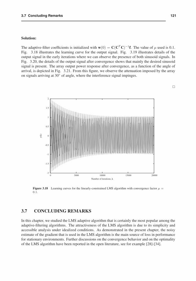
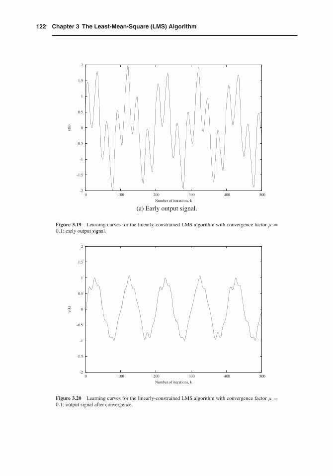
The adaptive-filter coefficients is initialized with w(0) = C(CTC)−1f. The value of μ used is 0.1.Fig. 3.18 illustrates the learning curve for the output signal. Fig. 3.19 illustrates details of theoutput signal in the early iterations where we can observe the presence of both sinusoid signals. InFig. 3.20, the details of the output signal after convergence shows that mainly the desired sinusoidsignal is present. The array output power response after convergence, as a function of the angle ofarrival, is depicted in Fig. 3.21. From this figure, we observe the attenuation imposed by the arrayon signals arriving at 30◦ of angle, where the interference signal impinges.

�

-2

-1.5

-1

-0.5

0

0.5

1

1.5

2

0 5000 10000 15000 20000

y(k)


Figure 3.18 Learning curves for the linearly-constrained LMS algorithm with convergence factor μ =0.1.

3.7 CONCLUDING REMARKS

In this chapter, we studied the LMS adaptive algorithm that is certainly the most popular among theadaptive-filtering algorithms. The attractiveness of the LMS algorithm is due to its simplicity andaccessible analysis under idealized conditions. As demonstrated in the present chapter, the noisyestimate of the gradient that is used in the LMS algorithm is the main source of loss in performancefor stationary environments. Further discussions on the convergence behavior and on the optimalityof the LMS algorithm have been reported in the open literature, see for example [28]-[34].


-2

-1.5

-1

-0.5

0

0.5

1

1.5

2

0 100 200 300 400 500

y(k)


(a) Early output signal.

Figure 3.19 Learning curves for the linearly-constrained LMS algorithm with convergence factor μ =0.1; early output signal.

-2

-1.5

-1

-0.5

0

0.5

1

1.5

2

0 100 200 300 400 500

y(k)


Figure 3.20 Learning curves for the linearly-constrained LMS algorithm with convergence factor μ =0.1; output signal after convergence.

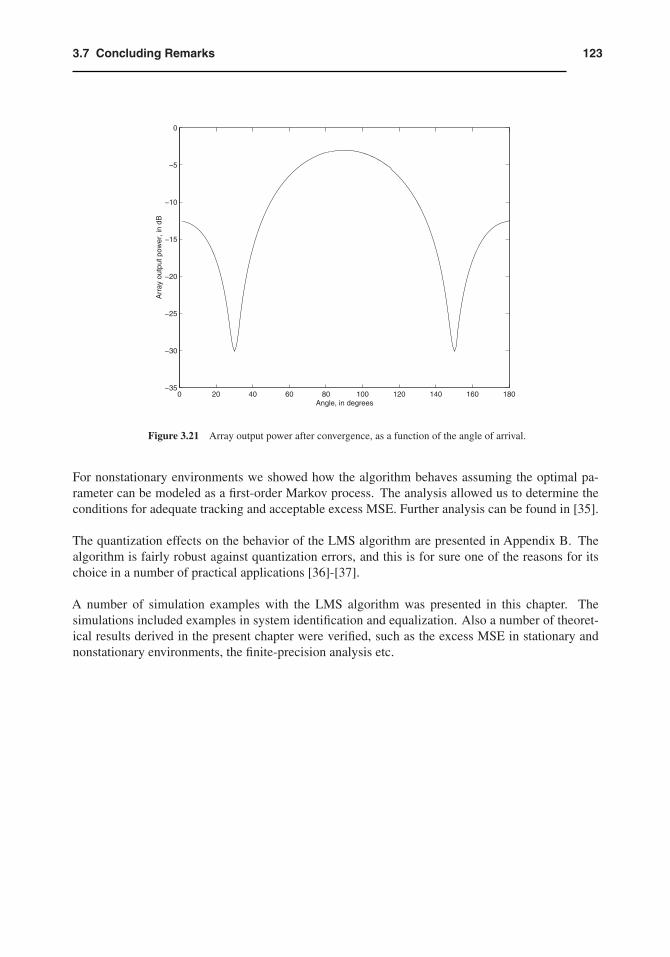
1233.7 Concluding Remarks

0 20 40 60 80 100 120 140 160 180−35

−30

−25

−20

−15

−10

−5

0

Angle, in degrees

Arr

ay o

utpu

t pow

er, i

n dB

Figure 3.21 Array output power after convergence, as a function of the angle of arrival.

For nonstationary environments we showed how the algorithm behaves assuming the optimal pa-rameter can be modeled as a first-order Markov process. The analysis allowed us to determine theconditions for adequate tracking and acceptable excess MSE. Further analysis can be found in [35].

The quantization effects on the behavior of the LMS algorithm are presented in Appendix B. Thealgorithm is fairly robust against quantization errors, and this is for sure one of the reasons for itschoice in a number of practical applications [36]-[37].

A number of simulation examples with the LMS algorithm was presented in this chapter. Thesimulations included examples in system identification and equalization. Also a number of theoret-ical results derived in the present chapter were verified, such as the excess MSE in stationary andnonstationary environments, the finite-precision analysis etc.


3.8 REFERENCES

1. B. Widrow and M. E. Hoff, “Adaptive switching circuits,” WESCOM Conv. Rec., pt. 4, pp.96-140, 1960.

2. B. Widrow, J. M. McCool, M. G. Larimore, and C. R. Johnson, Jr., “Stationary and nonstationarylearning characteristics of the LMS adaptive filters,” Proceedings of the IEEE, vol. 64, pp.1151-1162, Aug. 1976.

3. G. Ungerboeck, “Theory on the speed of convergence in adaptive equalizers for digital com-munication,” IBM Journal on Research and Development, vol. 16, pp. 546-555, Nov. 1972.

4. J. E. Mazo, “On the independence theory of equalizer convergence,” The Bell System TechnicalJournal, vol. 58, pp. 963-993, May 1979.

5. B. Widrow and S. D. Stearns, Adaptive Signal Processing, Prentice Hall, Englewood Cliffs, NJ,1985.

6. S. Haykin, Adaptive Filter Theory, Prentice Hall, Englewood Cliffs, NJ, 4th edition, 2002.

7. M. G. Bellanger, Adaptive Digital Filters and Signal Analysis, Marcel Dekker, Inc., New York,NY, 2nd edition, 2001.

8. D. C. Farden, “Tracking properties of adaptive signal processing algorithms,” IEEE Trans. onAcoust., Speech, and Signal Processing, vol. ASSP-29, pp. 439-446, June 1981.

9. B. Widrow and E. Walach, “On the statistical efficiency of the LMS algorithm with nonstationaryinputs,” IEEE Trans. on Information Theory, vol. IT-30, pp. 211-221, March 1984.

10. O. Macchi, “Optimization of adaptive identification for time varying filters,” IEEE Trans. onAutomatic Control, vol. AC-31, pp. 283-287, March 1986.

11. A. Benveniste, “Design of adaptive algorithms for the tracking of time varying systems,” Int. J.Adaptive Control and Signal Processing, vol. 1, pp. 3-29, Jan. 1987.

12. W. A. Gardner, “Nonstationary learning characteristics of the LMS algorithm,” IEEE Trans. onCircuits and Systems, vol. CAS-34, pp. 1199-1207, Oct. 1987.

13. A. Papoulis, Probability, Random Variables, and Stochastic Processes, McGraw Hill, NewYork,NY, 3rd edition, 1991.

14. F. J. Gantmacher, The Theory of Matrices, Chelsea Publishing Company, vol. 2, NewYork, NY,1964.

15. G. H. Golub and C. F. Van Loan, Matrix Computations, John Hopkins University Press, Balti-more, MD, 3rd edition, 1996.

16. V. Solo, “The limiting behavior of LMS,” IEEE Trans. on Acoust., Speech, and Signal Process-ing, vol-37, pp. 1909-1922, Dec. 1989.

17. N. J. Bershad and O. M. Macchi, “Adaptive recovery of a chirped sinusoid in noise, Part 2:Performance of the LMS algorithm,” IEEE Trans. on Signal Processing, vol. 39, pp. 595-602,March 1991.

1253.8 References

18. D. H. Brandwood, “A complex gradient operator and its application in adaptive array theory,”IEE Proceedings Parts F and G, vol. 130, pp. 11-16, Feb. 1983.

19. A. Hjørungnes and D. Gesbert, “Complex-valued matrix differentiation: Techniques and keyresults,” IEEE Trans. on Signal Processing, vol. 55, pp. 2740-2746, June 2007.

20. D. G. Manolakis, V. K. Ingle, and S. M. Kogon, Statistical and Adaptive Signal Processing,McGraw Hill, New York, NY, 2000.

21. V. H. Nascimento andA. H. Sayed, “On the learning mechanism of adaptive filters,” IEEE Trans.on Signal Processing, vol. 48, pp. 1609-1625, June 2000.

22. O. Macchi and E. Eweda, “Second-order convergence analysis of stochastic adaptive linearfilter,” IEEE Trans. on Automatic Control, vol. AC-28, pp. 76-85, March 1983.

23. S. Florian and A. Feuer, “Performance analysis of the LMS algorithm with a tapped delayline (two-dimensional case),” IEEE Trans. on Acoust., Speech, and Signal Processing, vol.ASSP-34, pp. 1542-1549, Dec. 1986.

24. O. L. Frost III, “An algorithm for linearly constrained adaptive array processing,” Proceedingsof the IEEE, vol. 60, pp. 926-935, Aug. 1972.

25. J. A. Apolinario Jr., S. Werner, T. I. Laakso, and P. S. R. Diniz, “Constrained normalizedadaptive filtering for CDMA mobile communications,” Proc. 1998 EUSIPCO-European SignalProcessing Conference, Rhodes, Greece, pp. 2053-2056, Sept. 1998.

26. J. A. Apolinario Jr., M. L. R. de Campos, and C. P. Bernal O., “The Constrained conjugate-gradient algorithm,”IEEE Signal Processing Letters, vol. 7, pp. 351-354, Dec. 2000.

27. M. L. R. de Campos, S. Werner, and J. A. Apolinario, Jr., “Constrained adaptation algorithmsemploying Householder transformation,” IEEE Transactions on Signal Processing, vol. 50, pp.2187-2195, Sept. 2002.

28. A. Feuer and E. Weinstein, “Convergence analysis of LMS filters with uncorrelated Gaussiandata,” IEEE Trans. on Acoust., Speech, and Signal Processing, vol. ASSP-33, pp. 222-230,Feb. 1985.

29. D. T. Slock, “On the convergence behavior of the LMS and normalized LMS algorithms,” IEEETrans. on Signal Processing, vol. 40, pp. 2811-2825, Sept. 1993.

30. W. A. Sethares, D. A. Lawrence, C. R. Johnson, Jr., and R. R. Bitmead, “Parameter drift in LMSadaptive filters,” IEEE Trans. on Acoust., Speech, and Signal Processing, vol. ASSP-34, pp.868-878, Aug. 1986.

31. S. C. Douglas, “Exact expectation analysis of the LMS adaptive filter,” IEEE Trans. on SignalProcessing, vol. 43, pp. 2863-2871, Dec. 1995.

32. H. J. Butterweck, “Iterative analysis of the state-space weight fluctuations in LMS-type adaptivefilters,” IEEE Trans. on Signal Processing, vol. 47, pp. 2558-2561, Sept. 1999.

33. B. Hassibi, A. H. Sayed, and T. Kailath, “H∞ optimality of the LMS Algorithm,” IEEE Trans.on Signal Processing, vol. 44, pp. 267-280, Feb. 1996.


34. O. J. Tobias, J. C. M. Bermudez, and N. J. Bershad, “Mean weight behavior of the filtered-XLMS algorithm,” IEEE Trans. on Signal Processing, vol. 48, pp. 1061-1075, April 2000.

35. V. Solo, “The error variance of LMS with time varying weights,” IEEE Trans. on SignalProcessing, vol. 40, pp. 803-813, April 1992.

36. S. U. Qureshi, “Adaptive Equalization,” Proceedings of the IEEE, vol-73, pp. 1349-1387, Sept.1985.

37. M. L. Honig, “Echo cancellation of voiceband data signals using recursive least squares andstochastic gradient algorithms,” IEEE Trans. on Communications, vol. COM-33, pp. 65-73,Jan. 1985.

38. V. H. Nascimento and J. C. M. Bermudez, “Probability of divergence for the least-mean fourthalgorithm,” IEEE Trans. on Signal Processing, vol. 54, pp. 1376-1385, April 2006.

3.9 PROBLEMS

1. The LMS algorithm is used to predict the signal x(k) = cos(πk/3) using a second-order FIRfilter with the first tap fixed at 1, by minimizing the mean squared value of y(k). Calculate anappropriate μ, the output signal, and the filter coefficients for the first 10 iterations. Start withwT (0) = [1 0 0].

2. The signalx(k) = −0.85x(k − 1) + n(k)

is applied to a first-order predictor, where n(k) is Gaussian white noise with variance σ2n = 0.3.

(a) Compute the Wiener solution.

(b) Choose an appropriate value for μ and plot the convergence path for the LMS algorithm onthe MSE error surface.

(c) Plot the learning curves for the MSE and the filter coefficients in a single run as well as forthe average of 25 runs.

3. Assuming it is desired to minimize the objective functionE[e4(k)] utilizing a stochastic gradienttype of algorithm such as the LMS. The resulting algorithm is called least-mean fourth algorithm[38]. Derive this algorithm.

4. The data-reusing LMS algorithm has the following updating equation

el(k) = d(k)− wTl (k)x(k)

wl+1(k) = wl(k) + 2μel(k)x(k) (3.102)

for l = 0, 1, . . . , L− 1, and

w(k + 1) = wL(k) = wL−1(k) + 2μeL−1(k)x(k) (3.103)

where w0(k) = w(k).

1273.9 Problems



(c) Compare its convergence speed and computational complexity with the LMS algorithm.

5. The momentum LMS algorithm has the following updating equation

w(k + 1) = w(k) + 2μe(k)x(k) + γ[w(k)−w(k − 1)] (3.104)

for |γ| < 1.



(c) Show that this algorithm can have faster convergence and higher misadjustment than theLMS algorithm.

6. An LMS algorithm can be updated in a block form. For a block of length 2 the updatingequations have the following form.[

e(k)e(k − 1)

]=[

d(k)d(k − 1)

]−[

xT (k)w(k)xT (k − 1)w(k − 1)

]

=[

d(k)d(k − 1)

]−[

xT (k)xT (k − 1)

]w(k − 1)

−[

0 2μxT (k)x(k − 1)0 0

] [e(k)

e(k − 1)

]

This relation, in a more compact way, is equivalent to[e(k)

e(k − 1)

]=[

1 −2μxT (k)x(k − 1)0 1

]{[d(k)

d(k − 1)

]−[

xT (k)xT (k − 1)

]w(k − 1)

}(3.105)

Derive an expression for a block of length L+ 1.

7. Use the LMS algorithm to identify a system with the transfer function given below. The inputsignal is a uniformly distributed white noise with variance σ2

x = 1, and the measurement noiseis Gaussian white noise uncorrelated with the input with variance σ2

n = 10−3. The adaptivefilter has 12 coefficients.

H(z) =1− z−12

1− z−1

(a) Calculate the upper bound for μ (μmax) to guarantee the algorithm stability.(b) Run the algorithm for μmax/2, μmax/10, and μmax/50. Comment on the convergencebehavior in each case.(c) Measure the misadjustment in each example and compare with the results obtained byequation (3.50).(d) Plot the obtained FIR filter frequency response at any iteration after convergence is achievedand compare with the unknown system.


8. Repeat the previous problem using an adaptive filter with 8 coefficients and interpret the results.

9. Repeat problem 2 in case the input signal is a uniformly distributed white noise with varianceσ2nx

= 0.5 filtered by an all-pole filter given by

H(z) =z

z − 0.9

10. Perform the equalization of a channel with the following impulse response

h(k) = ku(k)− (2k − 9)u(k − 5) + (k − 9)u(k − 10)

Using a known training signal that consists of a binary (-1,1) random signal, generated byapplying a white noise to a hard limiter (the output is 1 for positive input samples and -1 fornegative). An additional Gaussian white noise with variance 10−2 is present at the channeloutput.(a) Apply the LMS with an appropriate μ and find the impulse response of an equalizer with100 coefficients.(b) Convolve one of the equalizer’s impulse response after convergence with the channel impulseresponse and comment on the result.

11. Under the assumption that the elements of x(k) are jointly Gaussian, show that equation (3.24)is valid.

12. In a system identification problem the input signal is generated by an autoregressive processgiven by

x(k) = −1.2x(k − 1)− 0.81x(k − 2) + nx(k)

where nx(k) is zero-mean Gaussian white noise with variance such that σ2x = 1. The unknown

system is described by

H(z) = 1 + 0.9z−1 + 0.1z−2 + 0.2z−3

The adaptive filter is also a third-order FIR filter, and the additional noise is zero-mean Gaussianwhite noise with variance σ2

n = 0.04. Using the LMS algorithm:(a) Choose an appropriate μ, run an ensemble of 20 experiments, and plot the average learningcurve.(b) Plot the curve obtained using equations (3.41), (3.45), and (3.46), and compare the results.(c) Compare the measured and theoretical values for the misadjustment.(d) Calculate the time constants τwi and τei, and the expected number of iterations to achieveconvergence.

13. In a nonstationary environment the optimal coefficient vector is described by

wo(k) = −λ1wo(k − 1)− λ2wo(k − 2) + nw(k)

where nw(k) is a vector whose elements are zero-mean Gaussian white processes with varianceσ2

w. Calculate the elements of the lag-error vector.

14. Repeat the previous problem for

wo(k) = λwwo(k − 1) + (1− λw)nw(k)

1293.9 Problems

15. The LMS algorithm is applied to identify a 7th-order time-varying unknown system whosecoefficients are first-order Markov processes with λw = 0.999 and σ2

w = 0.001. The initialtime-varying-system multiplier coefficients are

wTo =

[0.03490 − 0.011 − 0.06864 0.22391 0.55686 0.35798 − 0.0239 − 0.07594]

The input signal is Gaussian white noise with variance σ2x = 0.7, and the measurement noise is

also Gaussian white noise independent of the input signal and of the elements of nw(k), withvariance σ2

n = 0.01.(a) For μ = 0.05, compute the excess MSE.(b) Repeat (a) for μ = 0.01.(c) Compute μopt and comment if it can be used.

16. Simulate the experiment described in problem 15, measure the excess MSE, and compare to thecalculated results.

17. Reduce the value of λw to 0.97 in problem 15, simulate, and comment on the results.

18. Suppose a 15th-order FIR digital filter with multiplier coefficients given below is identifiedthrough an adaptive FIR filter of the same order using the LMS algorithm.(a) Considering that fixed-point arithmetic is used, compute the expected value for ||Δw(k)Q||2and ξ(k)Q, and the probable number of iterations before the algorithm stops updating, for thefollowing case:

Additional noise: white noise with variance σ2n = 0.0015

Coefficient wordlength: bc = 16 bitsSignal wordlength: bd = 16 bitsInput signal: Gaussian white noise with variance σ2

x = 0.7μ = 0.01

Hint: Utilize the formulas for the time constant in the LMS algorithm and equation (B.28).(b) Simulate the experiment and plot the learning curves for the finite- and infinite-precisionimplementations.(c) Compare the simulated results with those obtained through the closed form formulas.

wTo = [0.0219360 0.0015786 − 0.0602449 − 0.0118907 0.13753790.0574545 − 0.3216703 − 0.5287203 − 0.2957797 0.0002043 0.290670−0.0353349 − 0.068210 0.0026067 0.0010333 − 0.0143593]

19. Repeat the above problem for the following cases(a) σ2

n = 0.01, bc = 12 bits, bd = 12 bits, σ2x = 0.7, μ = 2.0 10−3.

(b) σ2n = 0.1, bc = 10 bits, bd = 10 bits, σ2

x = 0.8, μ = 1.0 10−4.(c) σ2

n = 0.05, bc = 14 bits, bd = 14 bits, σ2x = 0.8, μ = 2.0 10−3.

20. Find the optimal value of μ (μopt) that minimizes the excess MSE given in equation (B.32), andcompute for μ = μopt the expected value of ||Δw(k)Q||2 and ξ(k)Q for the examples describedin problem 19.

21. Repeat problem 18 for the case where the input signal is a first-order Markov process withλx = 0.95.


22. A digital channel model can be represented by the following impulse response:

[−0.001 − 0.002 0.002 0.2 0.6 0.76 0.9 0.78 0.67 0.580.45 0.3 0.2 0.12 0.06 0 − 0.2 − 1 − 2 − 1 0 0.1]

The channel is corrupted by Gaussian white noise with power spectrum given by

|S(ejω)|2 = κ′|ω|3/2

where κ′ = 10−1.5. The training signal consists of independent binary samples (-1,1).

Design an FIR equalizer for this problem and use the LMS algorithm. Use a filter of order 50and plot the learning curve.

23. For the previous problem, using the maximum of 51 adaptive filter coefficients, implement aDFE equalizer and compare the results with those obtained with the FIR filter. Again use theLMS algorithm.

24. Implement with fixed-point arithmetic the DFE equalizer of problem 23, using the LMS algo-rithm with 12 bits of wordlength for data and coefficients.

25. Use the complex LMS algorithm to equalize a channel with the transfer function given below.The input signal is a four Quadrature Amplitude Modulation (QAM)5 signal representing a

randomly generated bit stream with the signal to noise ratio σ2x

σ2n

= 20 at the receiver end, that is,x(k) is the received signal without taking into consideration the additional channel noise. Theadaptive filter has 10 coefficients.

H(z) = (0.34− 0.27j) + (0.87 + 0.43j)z−1 + (0.34− 0.21j)z−2

(a) Calculate the upper bound for μ (μmax) to guarantee the algorithm stability.(b) Run the algorithm for μmax/2, μmax/10, and μmax/50. Comment on the convergencebehavior in each case.(c) Plot the real versus imaginary parts of the received signal before and after equalization.(d) Increase the number of coefficients to 20 and repeat the experiment in (c).

26. In a system identification problem the input signal is generated from a four QAM of the form

x(k) = xre(k) + jxim(k)

where xre(k) and xim(k) assume values ±1 randomly generated. The unknown system isdescribed by

H(z) = 0.32 + 0.21j+ (−0.3 + 0.7j)z−1 + (0.5− 0.8j)z−2 + (0.2 + 0.5j)z−3

The adaptive filter is also a third-order complex FIR filter, and the additional noise is zero-meanGaussian white noise with variance σ2

n = 0.4. Using the complex LMS algorithm, choose anappropriate μ, run an ensemble of 20 experiments, and plot the average learning curve.

5TheM -ary QAM constellation points are represented in by si = ai + jbi, with ai = ±d,±3d, . . . ,±(√M−1)d, and

bi = ±d,±3d, . . . ,±(√M−1)d. The parameter d is represents half of the distance between two points in the constellation.

Documents

THE LEAST-MEAN-SQUARE (LMS) ALGORITHMscs.etc.tuiasi.ro/iciocoiu/courses/PAS/course/course3/1.pdf · 78 Chapter 3 The Least-Mean-Square (LMS) Algorithm If good estimates of matrix