ESPResSo Tutorial

The Lattice Boltzmann Method inESPResSo: Polymer Diffusion and

Electroosmotic Flow

October 9, 2016Institute for Computational Physics, Stuttgart University

E

E_

_

_

_

_

_

_

_

_

_

+

xy

z

1

Before you start:With this tutorial you can get started using the Lattice-Boltzmann method for scien-tific applications. We give a brief introduction about the theory and how to use it inESPResSo. We have selected three interesting problems for which LB can be appliedand which are well understood. You can start with any of them.The tutorial is relatively long and working through it carefully is work for at least afull day. You can however get a glimpse of different aspects by starting to work onthe tasks.Note: LB can not be used as a black box. It is unavoidable to spend time learning thetheory and gaining practical experience.

Contents

1 Introduction 3

2 The LBM in brief 4

3 The LB interface in ESPResSo 7

4 Drag force on objects 10

5 Polymer Diffusion 11

6 Poiseuille flow ESPResSo 14

2

1 Introduction

In this tutorial, you will learn basics about the Lattice Boltzmann Method (LBM) with specialfocus on the application on soft matter simulations or more precisely on how to apply it incombination with molecular dynamics to take into account hydrodynamic solvent effects withoutthe need to introduce thousands of solvent particles.

The LBM – its theory as well as its applications – is still a very active field of research. Afteralmost 20 years of development there are many cases in which the LBM has proven to be fruitful,in other cases the LBM is considered promising, and in some cases it has not been of any help.We encourage you to contribute to the scientific discussion of the LBM because there is still alot that is unknown or only vaguely known about this fascinating method.

Tutorial Outline

This tutorial should enable you to start a scientific project applying the LB method withESPResSo. In the first part we summarize a few basic ideas behind LB and describe the in-terface. In the second part we suggest three different classic examples where hydrodynamics areimportant. These are

• Hydrodynamic resistance of settling particles. We measure the drag force of singleparticles and arrays of particles when sedimenting in solution.

• Polymer diffusion. We show that the diffusion of polymers is accelerated by hydrody-namic interactions.

• Poiseuille flow. We reproduce the flow profile between two walls.

Notes on the ESPResSo version you will need

With Version 3.1 ESPResSo has learned GPU support for LB. We recommend however version3.3, to have all features available. We absolutely recommend using the GPU code, as it is much(100x) faster than the CPU code.

For the tutorial you will have to compile in the following features:PARTIAL_PERIODIC, EXTERNAL_FORCES, CONSTRAINTS, ELECTROSTATICS,LB_GPU, LB_BOUNDARIES_GPU, LENNARD_JONES.

All necessary files for this tutorial are located in the directoryespresso/doc/tutorials/python/04-lattice_boltzmann/scripts.

3

2 The LBM in brief

Linearized Boltzmann equation

Here we want to repeat a few very basic facts about the LBM. You will find much better intro-ductions in various books and articles, e.g. [1, 2]. It will however help clarifying our choiceof words and we will eventually say something about the implementation in ESPResSo. It isvery loosely written, with the goal that the reader understands basic concepts and how they areimplemented in ESPResSo.

The LBM essentially consists of solving a fully discretized version of the linearized Boltz-mann equation. The Boltzmann equation describes the time evolution of the one particle distri-bution function f (x, p, t), which is the probability to find a molecule in a phase space volumedxdp at time t.The function f is normalized so that the integral over the whole phase space isthe total mass of the particles: ∫

f (x, p) dxdp = Nm,

where N denotes the particle number and m the particle mass. The quantity f(x, p) dxdpcorresponds to the mass of particles in this particular cell of the phase space, the population.

Discretization

The LBM discretizes the Boltzmann equation not only in real space (the lattice!) and time, butalso the velocity space is discretized. A surprisingly small number of velocities, in 3D usually19, is sufficient to describe incompressible, viscous flow correctly. Mostly we will refer tothe three-dimensional model with a discrete set of 19 velocities, which is conventionally calledD3Q19. These velocities, ~ci, are chosen so that they correspond to the movement from onelattice node to another in one time step. A two step scheme is used to transport informationthrough the system: In the streaming step the particles (in terms of populations) are transportedto the cell where they corresponding velocity points to. In the collision step, the distributionfunctions in each cell are relaxed towards the local thermodynamic equilibrium. This will bedescribed in more detail below.

The hydrodynamic fields, the density, the fluid momentum density, the pressure tensor canbe calculated straightforwardly from the populations: They correspond to the moments of thedistribution function:

ρ =∑

fi (1)

~j = ρ~u =∑

fi~ci (2)

Παβ =∑

fi~ciα~ci

β (3)

Here the Greek indices denotes the cartesian axis and the Latin indices indicate the number inthe disrete velocity set. Note that the pressure tensor is symmetric. It is easy to see that theseequations are linear transformations of the fi and that they carry the most important information.They are 10 independent variables, but this is not enough to store the full information of 19

4

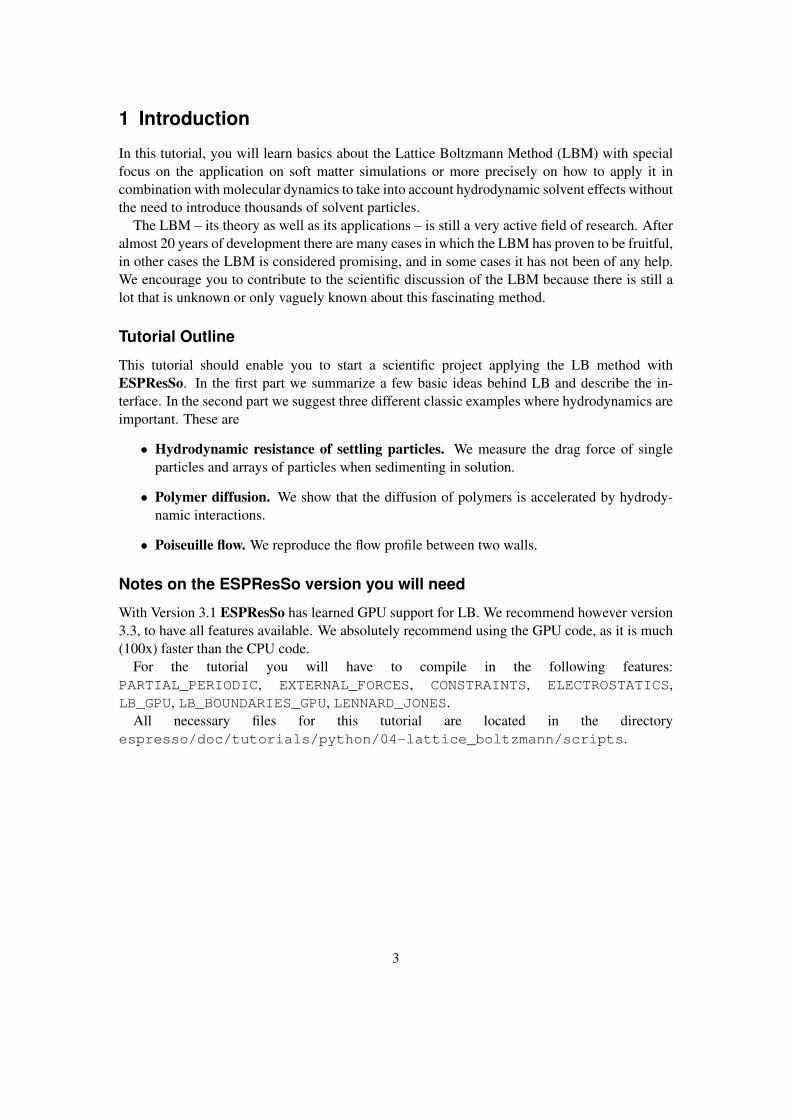
Figure 1: The 19 velocity vectors ~ci for a D3Q19 lattice. From the central grid point, the velocityvectors point towards all 18 nearest neighbours marked by filled circles. The 19thvelocity vector is the rest mode (zero velocity).

populations. Therefore 9 additional quantities are introduced. Together they form a differentbasis set of the 19-dimensional population space, the modes space and the modes are denotedby mi. The 9 extra modes are referred to as kinetic modes or ghost modes. It is possible toexplicitly write down the base transformation matrix, and its inverse and in the ESPResSo LBMimplementation this basis transformation is made for every cell in every LBM step. It is possibleto write a code that does not need this basis transformation, but it has been shown, that this onlycosts 20% of the computational time and allows for larger flexibility.

The second step: collision

The second step is the collision part, where the actual physics happens. For the LBM it is as-sumed that the collision process linearly relaxes the populations to the local equilibrium, thusthat it is a linear (=matrix) operator acting on the populations in each LB cell. It should conservethe particle number and the momentum. At this point it is clear why the mode space is helpful.A 19 dimensional matrix that conserves the first 4 modes (with the eigenvalue 1) is diagonal inthe first four rows and columns. Some struggling with lattice symmetries shows that four inde-pendent variables are anough to characterize the linear relaxation process so that all symmetriesof the lattice are obeyed. Two of them are closely related to the shear and bulk viscosity of thefluid, and two of them do not have a direct physical equivalent. They are just called relaxationrates of the kinetic modes.

The equilibrium distribution to which the populations relax is obtained from maximizing theinformation entropy

∑fi log fi under the constraint that the density and velocity take their

particular instantaneous values.In mode space the equilbrium distribution is calculated much from the local density and veloc-

5

ity. The kinetic modes 11-19 have the value 0 in equilibrium. The collision operator is diagonalin mode space and has the form

m?i = γi

(mi −meq

i

)+m

eqi .

Here m?i is the ith mode after the collision. In words we would say: Each mode is relaxed

towards it’s equilibrium value with a relaxation rate γi. The conserved modes are not relaxed,or, the corresponding relaxation parameter is one.

By symmetry consideration one finds that only four independent relaxation rates are allowed.We summarize them here.

m?i = γimi

γ1 = · · · = γ4 = 1

γ5 = γb

γ6 = · · · = γ10 = γs

γ11 = · · · = γ16 = γodd

γ17 = · · · = γ19 = γeven

To include hydrodynamic fluctuations of the fluid, random fluctuations are added to the non-conserved modes 4 . . . 19 on every LB node so that the LB fluid temperature is well defined andthe corresponding fluctuation formula, according to the fluctuation dissipation theorem holds.An extensive discussion of this topic is found in [3]

Particle coupling

Particles are coupled to the LB fluid with the force coupling: The fluid velocity at the positionof a particle is calculated by a multilinear interpolation and a force is applied on the particle thatis proportional to the velocity difference between particle and fluid:

~FD = −γ (v − u) (4)

The opposite force is distributed on the surrounding LB nodes. Additionally a random force isadded to maintain a constant temperature, according to the fluctuation dissipation theorem.

6

v(t)

u(1,t) u(2,t)

u(3,t) u(4,t)

u(r,t)

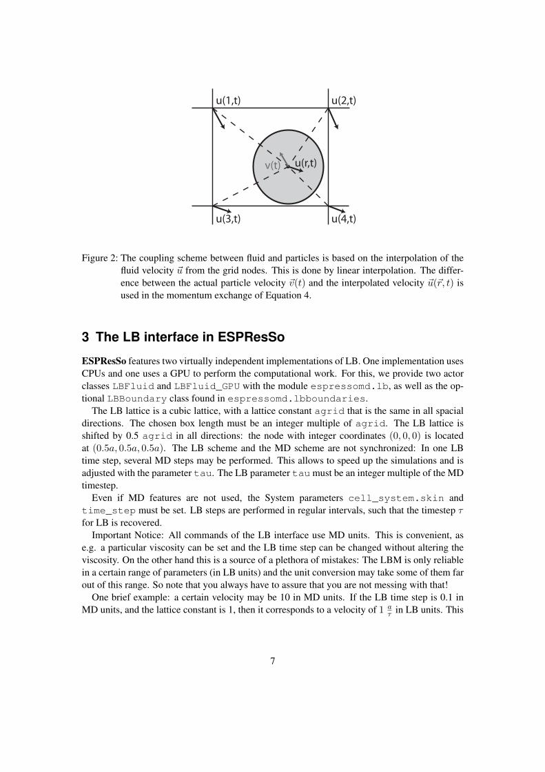
Figure 2: The coupling scheme between fluid and particles is based on the interpolation of thefluid velocity ~u from the grid nodes. This is done by linear interpolation. The differ-ence between the actual particle velocity ~v(t) and the interpolated velocity ~u(~r, t) isused in the momentum exchange of Equation 4.

3 The LB interface in ESPResSo

ESPResSo features two virtually independent implementations of LB. One implementation usesCPUs and one uses a GPU to perform the computational work. For this, we provide two actorclasses LBFluid and LBFluid_GPU with the module espressomd.lb, as well as the op-tional LBBoundary class found in espressomd.lbboundaries.

The LB lattice is a cubic lattice, with a lattice constant agrid that is the same in all spacialdirections. The chosen box length must be an integer multiple of agrid. The LB lattice isshifted by 0.5 agrid in all directions: the node with integer coordinates (0, 0, 0) is locatedat (0.5a, 0.5a, 0.5a). The LB scheme and the MD scheme are not synchronized: In one LBtime step, several MD steps may be performed. This allows to speed up the simulations and isadjusted with the parameter tau. The LB parameter tau must be an integer multiple of the MDtimestep.

Even if MD features are not used, the System parameters cell_system.skin andtime_step must be set. LB steps are performed in regular intervals, such that the timestep τfor LB is recovered.

Important Notice: All commands of the LB interface use MD units. This is convenient, ase.g. a particular viscosity can be set and the LB time step can be changed without altering theviscosity. On the other hand this is a source of a plethora of mistakes: The LBM is only reliablein a certain range of parameters (in LB units) and the unit conversion may take some of them farout of this range. So note that you always have to assure that you are not messing with that!

One brief example: a certain velocity may be 10 in MD units. If the LB time step is 0.1 inMD units, and the lattice constant is 1, then it corresponds to a velocity of 1 a

τ in LB units. This

7

is the maximum velocity of the discrete velocity set and therefore causes numerical instabilitieslike negative populations.

The LBFluid class

The LBFluid class provides an interface to the LB-Method in the ESPResSo core. Wheninitializing an object, one can pass the aforementioned parameters as keyword arguments. Pa-rameters are given in MD units. The available keyword arguments are:

dens The density of the fluid.agrid The lattice constant of the fluid. It is used to

determine the number of LB nodes per directionfrom box_l. They have to be compatible.

visc The kinematic viscositytau The time step of LB. It has to be an integer mul-

tiple of System.time_step.fric The friction coefficient γ for the coupling

scheme.ext_force An external force applied to every node. This is

given as a list, tuple or array with three compo-nents.

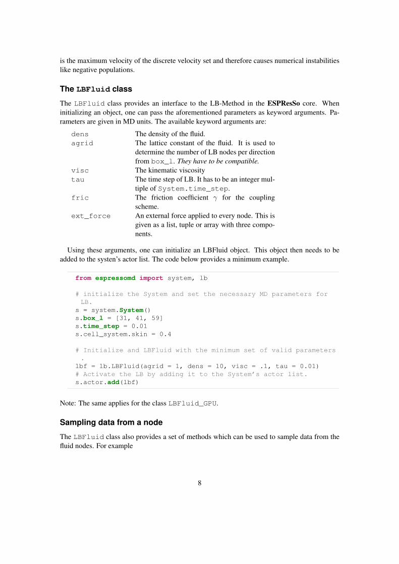
Using these arguments, one can initialize an LBFluid object. This object then needs to beadded to the systen’s actor list. The code below provides a minimum example.

from espressomd import system, lb

# initialize the System and set the necessary MD parameters forLB.

s = system.System()s.box_l = [31, 41, 59]s.time_step = 0.01s.cell_system.skin = 0.4

# Initialize and LBFluid with the minimum set of valid parameters.

lbf = lb.LBFluid(agrid = 1, dens = 10, visc = .1, tau = 0.01)# Activate the LB by adding it to the System’s actor list.s.actor.add(lbf)

Note: The same applies for the class LBFluid_GPU.

Sampling data from a node

The LBFluid class also provides a set of methods which can be used to sample data from thefluid nodes. For example

8

lbf[X,Y,Z].quantity

returns the quantity of the node with (X,Y, Z) coordinates. Note thatthe indexing in every direction starts with 0. The possible properties are:velocity the fluid velocity (list of three floats)pi the stress tensor (list of six floats: Πxx, Πxy,

Πyy, Πxz , Πyz , Πzz)pi_neq the nonequilbrium part of the stress tensor, com-

ponents as above.population the 19 populations of the D3Q19 lattice.boundary The boundary index.density the local density.

The LBBoundary class

The LBBoundary class represents a boundary on the LBFluid lattice. It is dependent on theclasses of the module espressomd.shapes as it derives its geometry from them. For theinitialization, the arguments shape and velocity are supported. The shape argument takesan object from the shapes module and the velocity argument expects a list, tuple or arraycontaining 3 floats. Setting the velocity will results in a slip boundary condition.

Note that the boundaries are not constructed through the periodic boundary. If, for example,one would set a sphere with its center in one of the corner of the boxes, a sphere fragment willbe generated. To avoid this, make sure the sphere, or any other boundary, fits inside the originalbox.

This part of the LB implementation is still experimental, so please tell us about your experi-ence with it. In general even the simple case of no-slip boundary is still an important researchtopic in the lb community and in combination with point particle coupling not much experienceexists. This means: Do research on that topic, play around with parameters and figure out whathappens.

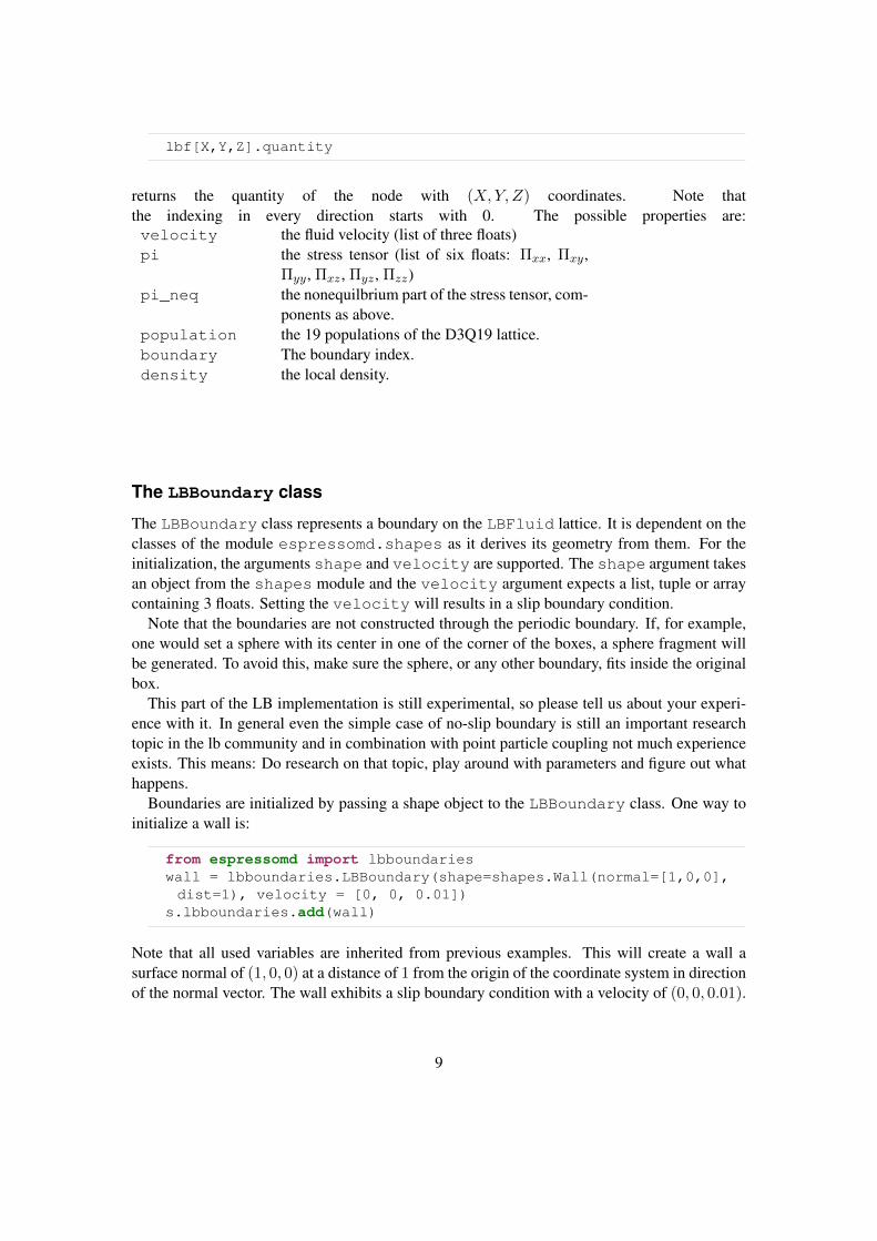
Boundaries are initialized by passing a shape object to the LBBoundary class. One way toinitialize a wall is:

from espressomd import lbboundarieswall = lbboundaries.LBBoundary(shape=shapes.Wall(normal=[1,0,0],dist=1), velocity = [0, 0, 0.01])

s.lbboundaries.add(wall)

Note that all used variables are inherited from previous examples. This will create a wall asurface normal of (1, 0, 0) at a distance of 1 from the origin of the coordinate system in directionof the normal vector. The wall exhibits a slip boundary condition with a velocity of (0, 0, 0.01).

9

For the a no-slip condition, leave out the velocity argument or set it so zero. Please refer to theuser guide for a complete list of constraints.

Currently only the so called link bounce back method is implemented, where the effectivehydrodynamic boundary is located midway between two nodes. This is the simplest and yet arather effective approach for boundary implementation. Using the shape objects distance func-tion, the nodes determine once during initialisation whether they are boundary or fluid nodes.

4 Drag force on objects

As a first test, we measure the drag force on different objects in a simulation box. Under lowReynolds number conditions, an object with velocity ~v experiences a drag force ~FD proportionalto the velocity:

~FD = −γ~v,

where γ is denoted the friction coefficient. In general γ is a tensor thus the drag force is generallynot parallel to the velocity. For spherical particles the drag force is given by Stokes’ law:

~FD = −6πηa~v,

where a is the radius of the sphere.In this task you will measure the drag force on falling objects with LB and ESPResSo. In

the sample script lb_stokes_force.py a spherical object at rest is centered in a squarechannel. Bounce back boundary conditions are assumed on the sphere. At the channel boundarythe velocity is fixed by using appropriate boundary conditions. Within a few hundred or thousandintegration steps a steady state develops and the force on the sphere converges.

Radius dependence of the drag force

Measure the drag force for three different input radii of the sphere. How good is the agreementwith Stokes’ law? Calculate an effective radius from Stokes’ law and the drag force measuredin the simulation. Is there a clear relation to the input radius? Remember how the bounce backboundary condition work and how good spheres can be represented by them.

Visualization of the flow field

The script produces vtk files of the flow field. Visualize the flow field with paraview. Openparaview by typing it on the command line. Make sure you are in the folder where the filesare located. So the agenda is:

• Click in the menu File, Open...

• Choose the files with flow field fluid...vtk

• Click Apply

10

• Add a stream tracer filter Filters, Alphabetical, Stream tracer

• Change the seed type from point source to high resolution line source

• Click Apply

• Rotate the visualization box to see the stream lines.

• Use the play button in the bar below the menu bar to show the time evolution.

System size dependence

Measure the drag force for a fixed radius but varying system size. Does the drag force increaseof decrease with the system size? Can you find a qualitative explanation?

5 Polymer Diffusion

In these exercises we want to use the LBM-MD-Hybrid to reproduce a classic result of polymerphysics: The dependence of the diffusion coefficient of a polymer on its chain length. If nohydrodynamic interactions are present, one expects a scaling law D ∝ N−1 and if they arepresent, a scaling law D ∝ N−ν is expected. Here ν is the Flory exponent that plays a veryprominent role in polymer physics. It has a value of ∼ 3/5 in good solvent conditions in 3D.Discussions of these scaling laws can be found in polymer physics textbooks like [4–6].

The reason for the different scaling law is the following: When being transported, everymonomer creates a flow field that follows the direction of its motion. This flow field makes iteasier for other monomers to follow its motion. This makes a polymer long enough diffuse morelike compact object including the fluid inside it, although it does not have clear boundaries. Itcan be shown that its motion can be described by its hydrodynamic radius. It is defined as:

〈 1

Rh〉 = 〈 1

N2

∑i 6=j

1

|ri − rj |〉 (5)

This hydrodynamic radius exhibits the scaling law Rh ∝ Nν and the diffusion coefficient oflong polymer is proportional to its inverse. For shorter polymers there is a transition region. Itcan be described by the Kirkwood-Zimm model:

D =D0

N+kBT

6πη〈 1

Rh〉 (6)

Here D0 is the monomer diffusion coefficient and η the viscosity of the fluid. For a finite systemsize the second part of the diffusion is subject of a 1/L finite size effect, because hydrodynamicinteractions are proportional to the inverse distance and thus long ranged. It can be taken intoaccount by a correction:

D =D0

N+kBT

6πη〈 1

Rh〉(

1− 〈RhL〉)

(7)

11

It is quite difficult to prove this formula with good accuracy. It will need quite some computertime and a careful analysis. So please don’t be too disappointed if you don’t manage to do so.

We want to determine the diffusion coefficient from the mean square distance that a particletravels in the time t. For large t it is be proportional to the time and the diffusion coefficientoccurs as prefactor:

∂〈r2 (t)〉∂t

= 2dD. (8)

Here d denotes the dimensionality of the system, in our case 3. This equation can be foundin virtually any simulation textbook, like [7]. We will therefore set up a polymer in an LBfluid, simulate for an appropriate amount of time, calculate the mean square displacement as afunction of time and obtain the diffusion coefficient from a linear fit. However we make a coupleof steps in between and divide the full problem into subproblems that allow to (hopefully) fullyunderstand the process.

5.1 Step 1: Diffusion of a single particle

Our first step is to investigate the diffusion of a single particle that is coupled to an LB fluid bythe point coupling method. Take a look at the script single_particle_diffusion.py.The script takes the LB-friction coefficient as an argument. Start with an friction coefficient of1.0:

/ p a t h / t o / p y p r e s s o s i n g l e _ p a r t i c l e _ d i f f u s i o n . py 1 . 0

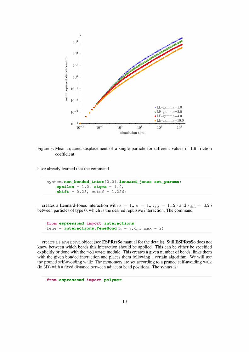
In this script an LB fluid and a single particle are created and thermalized. The randomforces on the particle and within the LB fluid will cause the particle to move. The mean squareddisplacement is calculated during the simulation via a multiple-tau correlator. Run the simulationscript and plot the output data msd_1.0.dat. To load the file into a numpy array, one can usenumpy.loadtxt. Zoom in on the origin of the plot. What do you see for short times? Whatdo you see on a longer time scale? Produce a double-logarithmic plot to assess the power law.

Can you give an explanation for the quadratic time dependency for short times? Use the func-tion curve_fit from the module scipy.optimize to produce a fit for the linear regimeand determine the diffusion coefficient.

Run the simulation again with different values for the friction coefficient, e.g. 1. 2. 4. 10.Calculate the diffusion coefficient for all cases and plot them as a function of γ. What relationdo you observe?

5.2 Step 2: Diffusion of a polymer

One of the typical applications of ESPResSo is the simulation of polymer chains with a bead-spring-model. For this we need a repulsive interaction between all beads, for which one usuallytakes a shifted and truncated Lennard-Jones (so called Weeks-Chandler-Anderson) interaction,and additionally a bonded interaction between adjacent beads to hold the polymer together. You

12

10−2 10−1 100 101 102 10310−4

10−3

10−2

10−1

100

101

102

103

simulation time

meansquared

displacement

LB-gamma=1.0LB-gamma=2.0LB-gamma=4.0LB-gamma=10.0

Figure 3: Mean squared displacement of a single particle for different values of LB frictioncoefficient.

have already learned that the command

system.non_bonded_inter[0,0].lennard_jones.set_params(epsilon = 1.0, sigma = 1.0,shift = 0.25, cutof = 1.226)

creates a Lennard-Jones interaction with ε = 1., σ = 1., rcut = 1.125 and εshift = 0.25between particles of type 0, which is the desired repulsive interaction. The command

from espressomd import interactionsfene = interactions.FeneBond(k = 7,d_r_max = 2)

creates a FeneBond object (see ESPResSo manual for the details). Still ESPResSo does notknow between which beads this interaction should be applied. This can be either be specifiedexplicitly or done with the polymer module. This creates a given number of beads, links themwith the given bonded interaction and places them following a certain algorithm. We will usethe pruned self-avoiding walk: The monomers are set according to a pruned self-avoiding walk(in 3D) with a fixed distance between adjacent bead positions. The syntax is:

from espressomd import polymer

13

# mpc: monomers per chainmpc = 30poly = polymer.Polymer(N_P=1, MPC = mpc, bond=fene, bond_length =1)

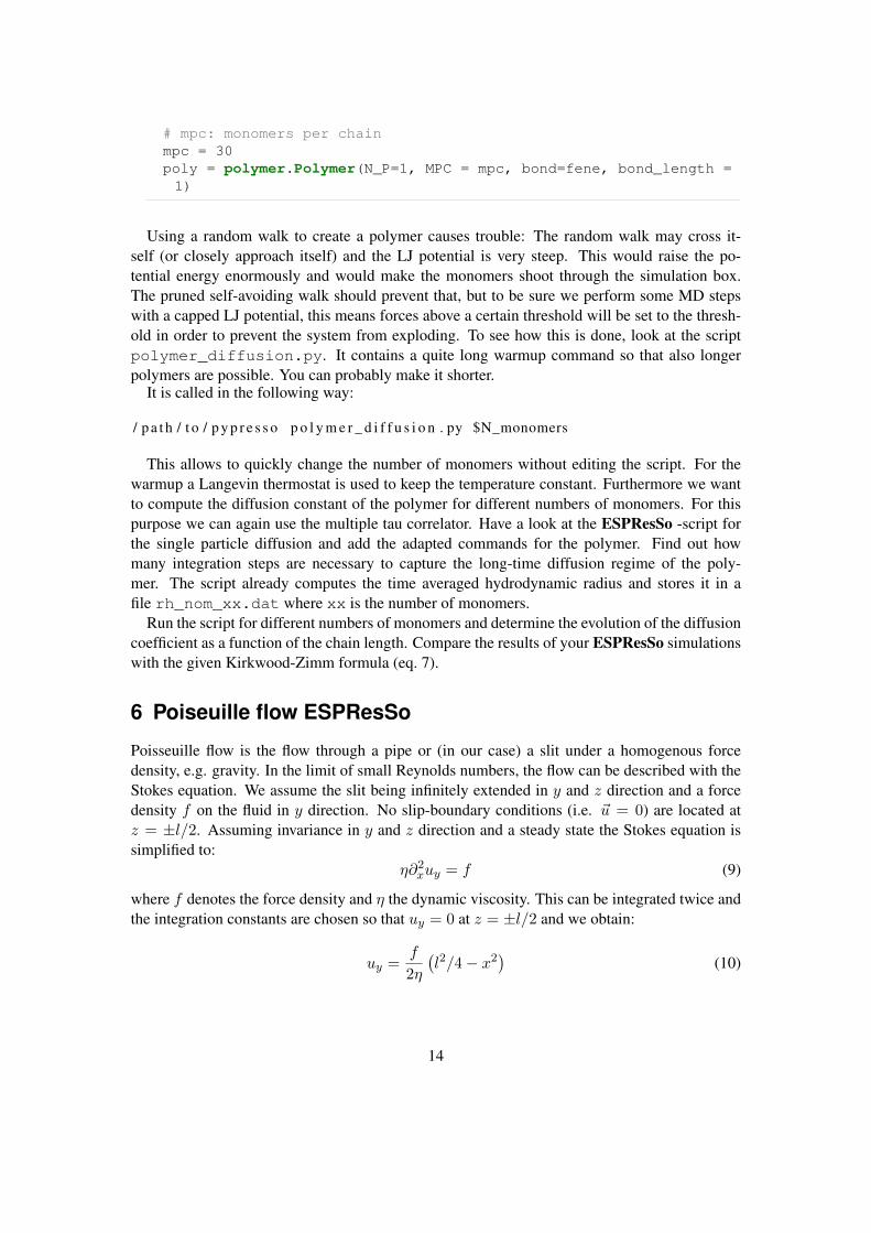
Using a random walk to create a polymer causes trouble: The random walk may cross it-self (or closely approach itself) and the LJ potential is very steep. This would raise the po-tential energy enormously and would make the monomers shoot through the simulation box.The pruned self-avoiding walk should prevent that, but to be sure we perform some MD stepswith a capped LJ potential, this means forces above a certain threshold will be set to the thresh-old in order to prevent the system from exploding. To see how this is done, look at the scriptpolymer_diffusion.py. It contains a quite long warmup command so that also longerpolymers are possible. You can probably make it shorter.

It is called in the following way:

/ p a t h / t o / p y p r e s s o p o l y m e r _ d i f f u s i o n . py $N_monomers

This allows to quickly change the number of monomers without editing the script. For thewarmup a Langevin thermostat is used to keep the temperature constant. Furthermore we wantto compute the diffusion constant of the polymer for different numbers of monomers. For thispurpose we can again use the multiple tau correlator. Have a look at the ESPResSo -script forthe single particle diffusion and add the adapted commands for the polymer. Find out howmany integration steps are necessary to capture the long-time diffusion regime of the poly-mer. The script already computes the time averaged hydrodynamic radius and stores it in afile rh_nom_xx.dat where xx is the number of monomers.

Run the script for different numbers of monomers and determine the evolution of the diffusioncoefficient as a function of the chain length. Compare the results of your ESPResSo simulationswith the given Kirkwood-Zimm formula (eq. 7).

6 Poiseuille flow ESPResSo

Poisseuille flow is the flow through a pipe or (in our case) a slit under a homogenous forcedensity, e.g. gravity. In the limit of small Reynolds numbers, the flow can be described with theStokes equation. We assume the slit being infinitely extended in y and z direction and a forcedensity f on the fluid in y direction. No slip-boundary conditions (i.e. ~u = 0) are located atz = ±l/2. Assuming invariance in y and z direction and a steady state the Stokes equation issimplified to:

η∂2xuy = f (9)

where f denotes the force density and η the dynamic viscosity. This can be integrated twice andthe integration constants are chosen so that uy = 0 at z = ±l/2 and we obtain:

uy =f

2η

(l2/4− x2

)(10)

14

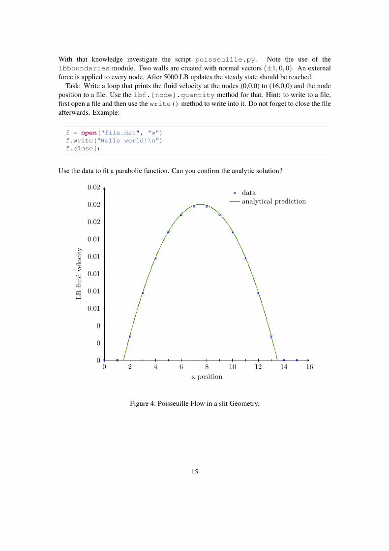
With that knowledge investigate the script poisseuille.py. Note the use of thelbboundaries module. Two walls are created with normal vectors (±1, 0, 0). An externalforce is applied to every node. After 5000 LB updates the steady state should be reached.

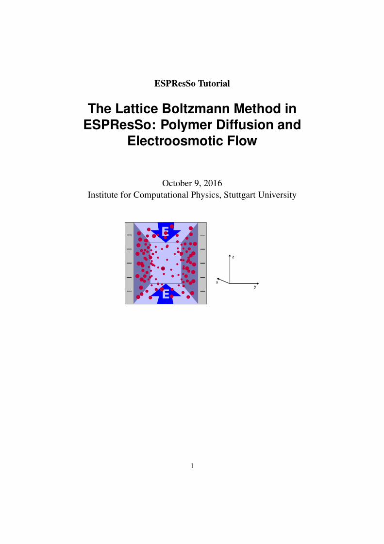
Task: Write a loop that prints the fluid velocity at the nodes (0,0,0) to (16,0,0) and the nodeposition to a file. Use the lbf.[node].quantity method for that. Hint: to write to a file,first open a file and then use the write() method to write into it. Do not forget to close the fileafterwards. Example:

f = open("file.dat", "w")f.write("Hello world!\n")f.close()

Use the data to fit a parabolic function. Can you confirm the analytic solution?

0 2 4 6 8 10 12 14 160

0

0

0.01

0.01

0.01

0.01

0.01

0.02

0.02

0.02

x position

LB

flu

idve

loci

ty

dataanalytical prediction

Figure 4: Poisseuille Flow in a slit Geometry.

15

References

[1] S Succi. The lattice Boltzmann equation for fluid dynamics and beyond. Clarendon Press,Oxford, 2001.

[2] B. Dünweg and A. J. C. Ladd. Advanced Computer Simulation Approaches for Soft MatterSciences III, chapter II, pages 89–166. Springer, 2009.

[3] B. Dünweg, U. Schiller, and A.J.C. Ladd. Statistical mechanics of the fluctuating lattice-boltzmann equation. Phys. Rev. E, 76:36704, 2007.

[4] P. G. de Gennes. Scaling Concepts in Polymer Physics. Cornell University Press, Ithaca,NY, 1979.

[5] M. Doi. Introduction do Polymer Physics. Clarendon Press, Oxford, 1996.

[6] Michael Rubinstein and Ralph H. Colby. Polymer Physics. Oxford University Press, Oxford,UK, 2003.

[7] Daan Frenkel and Berend Smit. Understanding Molecular Simulation. Academic Press,San Diego, second edition, 2002.

16