ESPResSo Tutorial

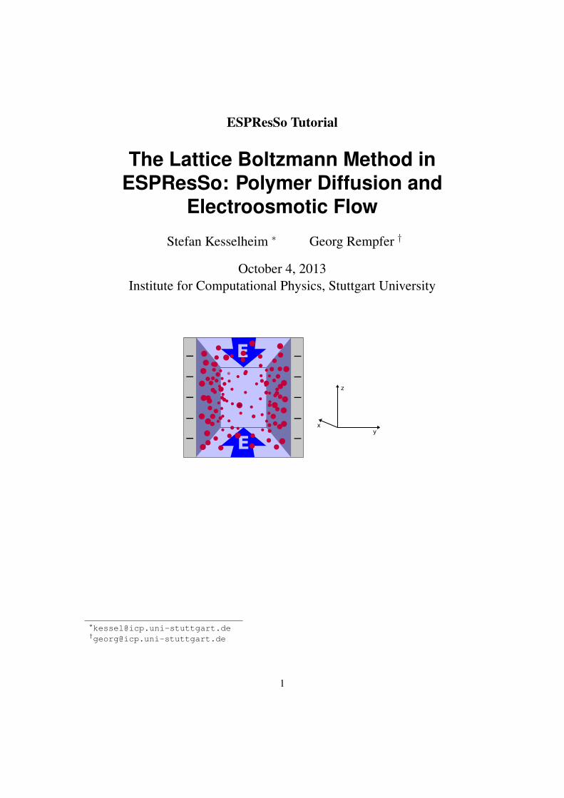
The Lattice Boltzmann Method inESPResSo: Polymer Diffusion and

Electroosmotic Flow

Stefan Kesselheim ∗ Georg Rempfer †

October 4, 2013Institute for Computational Physics, Stuttgart University

E

E_

_

_

_

_

_

_

_

_

_

+

xy

z

∗kessel@icp.uni-stuttgart.de†georg@icp.uni-stuttgart.de

1

Before you start:With this tutorial you can get started using the Lattice-Boltzmann method for sci-entific applications. We give a brief introduction about the theory and how to useit ESPResSo. We have selected three interesting problems, for which LB can beapplied, but which are well understood. You can start with any of them.The tutorial relatively long, and working through it carefully is work for at least a fullday. You can however get a glimpse of different aspects by starting to work on thetasks.Note: LB can not be used as a black box. It is unavoidable to spend time learning thetheory and gaining practical experience.

Contents

1 Introduction 3

2 The LBM in brief 4

3 The LB interface in ESPResSo 7

4 Drag force on objects 11

5 Polymer Diffusion 12

6 Electro-osmotic flow in a slit pore 16

2

1 Introduction

In this tutorial, you will learn basics about the Lattice Boltzmann Method (LBM) with specialfocus on the application on soft matter simulations, or more precisely on how to apply it incombination with molecular dynamics to take into account hydrodynamic solvent effects withoutthe need to introduce thousands of solvent particles.

The LBM – its theory as well as its applications – is still a very active field of research. Afteralmost 20 years of development there are many cases in which the LBM has proven to be fruitful,in other cases the LBM is considered promising, and in some cases it has not been of any help.We encourage you to contribute to the scientific discussion of the LBM because there is still alot that is unknown or only vaguely known about this fascinating method.

Tutorial Outline

This tutorial should enable you to start a scientific project applying the LB method withESPResSo. In the first part summarize a few basic ideas behind LB, and describe the inter-face. In the second part we suggest three different classic examples, where hydrodynamics areimportant. These are

• Hydrodynamic resistance of settling particles. We measure the drag force of singleparticles and arrays of particles when sedimenting in solution.

• Polymer diffusion. We show that the diffusion of polymers is accelerated by hydrody-namic interactions.

• Electroosmotic flow. We reproduce the flow pattern created by between charged wallswhen an electric field is applied.

Notes on the ESPResSo version you will need

With Version 3.1 ESPResSo has learned GPU support for LB. We recommend however version3.2, to have all features available. We absolutely recommend using the GPU code, as it is much(100x) faster than the CPU code.

For the tutorial you will have to compile in the following features:PARTIAL_PERIODIC, ELECTROSTATICS, EXTERNAL_FORCES, CONSTRAINTS,LB_GPU, LB_BOUNDARIES_GPU, LENNARD_JONES.

All necessary files for this tutorial are located in the directory lb_tutorial/src.

3

2 The LBM in brief

Linearized Boltzmann equation

Here we want to repeat a few very basic facts about the LBM. You will find much better intro-ductions in various books and articles, e.g. [1, 2]. It will however help clarifying our choiceof words and we will eventually say something about the implementation in ESPResSo. It isvery loosely written, with the goal that the reader understands basic concepts and how they areimplemented in ESPResSo.

The LBM essentially consists of solving a fully discretized version of the linearized Boltz-mann equation. The Boltzmann equation describes the time evolution of the one particle distri-bution function f (x, p, t), which is the probability to find a molecule in a phase space volumedxdp at time t.The function f is normalized so that the integral over the whole phase space isthe total mass of the particles: ∫

f (x, p) dxdp = Nm,

where N denotes the particle number and m the particle mass. The quantity f(x, p) dxdpcorresponds to the mass of particles in this particular cell of the phase space, the population.

Discretization

The LBM discretizes the Boltzmann equation not only in real space (the lattice!) and time, butalso the velocity space is discretized. A surprisingly small number of velocities, in 3D usually19, is sufficient to describe incompressible, viscous flow correctly. Mostly we will refer tothe three-dimensional model with a discrete set of 19 velocities, which is conventionally calledD3Q19. These velocities, ~ci, are chosen so that they correspond the movement from one latticenode to another in one time step. A two step scheme is used to transport information throughthe system: In the streaming step the particles (in terms of populations) are transported to thecell where they corresponding velocity points to. In the collision step, the distribution functionsin each cell are relaxed towards the local thermodynamic equilibrium. This will be described inmore detail below.

The hydrodynamic fields, the density, the fluid momentum density, the pressure tensor can becalculated straightforwardly from the populations: They correspond the to the moments of thedistribution function:

ρ =∑

fi (1)

~j = ρ~u =∑

fi~ci (2)

Παβ =∑

fi~ciα~ci

β (3)

Here the Greek indices denotes the cartesian axis and the Latin indices indicate the number inthe disrete velocity set. Note that the pressure tensor is symmetric. It is easy to see that theseequations are linear transformations of the fi and that they carry the most important information.They are 10 independent variables, but this is not enough to store the full information of 19

4

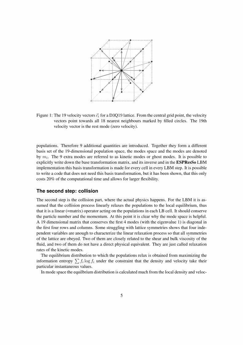
Figure 1: The 19 velocity vectors ~ci for a D3Q19 lattice. From the central grid point, the velocityvectors point towards all 18 nearest neighbours marked by filled circles. The 19thvelocity vector is the rest mode (zero velocity).

populations. Therefore 9 additional quantities are introduced. Together they form a differentbasis set of the 19-dimensional population space, the modes space and the modes are denotedby mi. The 9 extra modes are referred to as kinetic modes or ghost modes. It is possible toexplicitly write down the base transformation matrix, and its inverse and in the ESPResSo LBMimplementation this basis transformation is made for every cell in every LBM step. It is possibleto write a code that does not need this basis transformation, but it has been shown, that this onlycosts 20% of the computational time and allows for larger flexibility.

The second step: collision

The second step is the collision part, where the actual physics happens. For the LBM it is as-sumed that the collision process linearly relaxes the populations to the local equilibrium, thusthat it is a linear (=matrix) operator acting on the populations in each LB cell. It should conservethe particle number and the momentum. At this point it is clear why the mode space is helpful.A 19 dimensional matrix that conserves the first 4 modes (with the eigenvalue 1) is diagonal inthe first four rows and columns. Some struggling with lattice symmetries shows that four inde-pendent variables are anough to characterize the linear relaxation process so that all symmetriesof the lattice are obeyed. Two of them are closely related to the shear and bulk viscosity of thefluid, and two of them do not have a direct physical equivalent. They are just called relaxationrates of the kinetic modes.

The equilibrium distribution to which the populations relax is obtained from maximizing theinformation entropy

∑fi log fi under the constraint that the density and velocity take their

particular instantaneous values.In mode space the equilbrium distribution is calculated much from the local density and veloc-

5

ity. The kinetic modes 11-19 have the value 0 in equilibrium. The collision operator is diagonalin mode space and has the form

m?i = γi

(mi −meq

i

)+m

eqi .

Here m?i is the ith mode after the collision. In words we would say: Each mode is relaxed is

relaxed towards its equilibrium value with a relaxation rate γi. The conserved modes are notrelaxed, or, the corresponding relaxation parameter is one.

By symmetry consideration one finds that only four independent relaxation rates are allowed.We summarize them here.

m?i = γimi

γ1 = · · · = γ4 = 1

γ5 = γb

γ6 = · · · = γ10 = γs

γ11 = · · · = γ16 = γodd

γ17 = · · · = γ19 = γeven

To include hydrodynamic fluctuations of the fluid, random fluctuations are added to the non-conserved modes 4 . . . 19 on every LB node so that the LB fluid temperature is well defined andthe corresponding fluctuation formula, according to the fluctuation dissipation theorem holds.An extensive discussion of this topic is found in [3]

Particle coupling

Particles are coupled to the LB fluid with the force coupling: The fluid velocity at the positionof a a particle is, is calculated by a multilinear interpolation and a force is applied on the particlethat is proportional to the velocity difference between particle and fluid:

~FD = −γ (v − u) (4)

The opposite force is distributed on the surrounding LB nodes. Additionally a random force isadded to maintain a constant temperature, according to the fluctuation dissipation theorem.

6

v(t)

u(1,t) u(2,t)

u(3,t) u(4,t)

u(r,t)

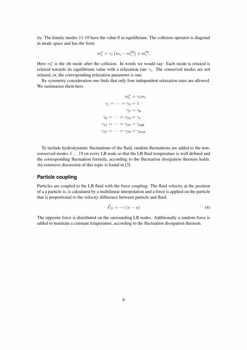
Figure 2: The coupling scheme between fluid and particles is based on the interpolation of thefluid velocity ~u from the grid nodes. This is done by linear interpolation. The differ-ence between the actual particle velocity ~v(t) and the interpolated velocity ~u(~r, t) isused in the momentum exchange of Equation 4.

3 The LB interface in ESPResSo

ESPResSo features two virtually independent implementations of LB. lbfluidThe LB lattice is a cubic lattice, with a lattice constant agrid that is the same in all spacial

directions. The chosen box length must be an integer multiple if agrid. The LB lattice isshifted by 0.5 agrid in all directions: the node with integer coordinates (0, 0, 0) is located at(0.5a, 0.5a, 0.5). The LB scheme and the MD scheme are not synchronized: In one LB timestep typically several MD steps are performed. This allows to speed up the simulations and isadjusted with the parameter tau. The LB parameter tau must be an integer multiple of the MDtimestep.

Even if MD features are not used, a few MD parameters must be set, although they are ir-relevant to the LB module. These is mainly skin, but also the MD timestep has to be set, asthe command integrate is used to propagate MD steps. LB steps are performed in regularintervals.

ESPResSo has three main commands for the LB module: lbfluid, lbnode, andlbboundary. lbfluid is mainly used to set up parameters and does everything that concernsthe whole fluid. lbnode involves readout and manipulation of single LB cells. lbboundaryallows to set boundaries, currently only the bounce back boundary method is implemented tomodel no-slip walls. Additionally the command thermostat lb is used to set the tempera-ture.

Important Notice: All commands of the LB interface use MD units. This is convenient, ase.g. a particular viscosity can be set and the LB time step can be changed without altering theviscosity. On the other hand this is a source of a plethora of mistakes: The LBM is only reliable

7

in a certain range of parameters (in LB units) and the unit conversion may take some of them farout of this range. So note that you always have to assure that you are not messing with that!

One brief example: a certain velocity may be 10 in MD units. If the LB time step is 0.1 inMD units, and the lattice constant is 1, then it corresponds to a velocity of 1 in LB units. Thisis the maximum velocity of the discrete velocity set and therefore causes numerical instabilitieslike negative populations.

The lbfluid command

The lbfluid command sets global parameters of the LBM. Every parameter is given in theform lbfluid name value. All parameters except for gamma_odd and gamma_evenare given in MD units. All parameters except for ext_force accept one scalar floating pointargument.dens The density of the fluid.grid The lattice constant of the fluid. It is used to

determine the number of LB nodes per directionfrom box_l. They have to be compatible.

visc The kinematic viscositytau The time step of LB. It has to be equal or larger

than the MD time step.friction The friction coefficient γ for the coupling

scheme.ext_force An external force applied to every node with

three components.gamma_odd Relaxation parameter for the odd kinetic modes.gamma_even Relaxation parameter for the even kinetic

modes.

A good starting point for an MD time step of 0.01 is the command line

l b f l u i d g r i d 1 . 0 dens 10 . v i s c . 1 t a u 0 . 0 1 f r i c t i o n 10 .

The lbnode command

The lbnode command allows to inspect and modify single LB nodes The general syntax is:

lbnode X Y Z command a rgumen t s

Note that the indexing in every direction starts with 0. The possible commands are:print Print one or several quantities to the TCL inter-

face.set Set one quantity to a particular value (can be a

vector)

8

For both commands you have to specify what quantity should be printed or modified. Print

allows the following arguments:

rho the density (scalar).u the fluid velocity (three floats: ux, uy, uz)pi the fluid velocity (six floats: Πxx, Πxy, Πyy,

Πxz , Πyz , Πzz)pi_neq the nonequilbrium part of the pressure tensor,

components as above.pop the 19 population (check the order from the

source code please).Example: The line

puts [ lbnode 0 0 0 p r i n t u ]

prints the fluid velocity in node 0 0 0 to the screen. The command set allows to change thedensity or fluid velocity in a single node. Setting the other quantities can easily be implemented.Example:

puts [ lbnode 0 0 0 s e t u 0 . 0 1 0 . 0 . ]

The lbboundary command

The lbboundary allows to set boundary conditions for the LB fluid. In general periodicboundary conditions are applied in all directions, and only if LB boundaries are constructedfinite geometries are used. This part of the LB implementation is still experimental, so pleasetell us about your experience with it. In general even the simple case of no-slip boundary is stillan important research topic in the lb community, and in combination with point particle couplingnot much experience exists. This means: Do research on that topic, play around with parametersand find out what happens.

The lbboundary command is supposed to resemble exactly the constraint commandof ESPResSo: Just replace the keyword constraint with the word lbboundary andESPResSo will create walls with the same shape as the corresponding constraint. Example:The commands

l b b o u n d a r y w a l l d i s t 1 . normal 1 . 0 . 0 .l b b o u n d a r y w a l l d i s t −9. normal −1. 0 . 0 .

create a channel with walls parallel to the yz plane with width 8.Currently only the so called link bounce back method is implemented, where the effective

hydrodynamic boundary is located midway between two nodes. This is the simplest and yet a

9

rather effective approach for boundary implementation. The lbboundary command checksfor every LB node if it is inside the constraint or outside and flags it as a boundary node or not.This means if the lattice constant is set to 1, the above command yields exactly the same as this:

l b b o u n d a r y w a l l 0 . 1 0 0 normal 1 . 0 . 0 .l b b o u n d a r y w a l l −8.1 0 0 normal −1. 0 . 0 .

This has to be kept in mind, when you use the LB boundaries.Currently only the shapes wall, sphere and cylinder are implemented, but to implement others

is straightforward. If you need them, please let us know.

10

4 Drag force on objects

As a first test, we measure the drag force on different objects in a simulation box. Und lowReynolds number conditions, a object with velocity ~v experiences a drag force ~FD proportionalto the velocity:

~FD = −γ~v,

where γ is denoted the friction coefficient. In general, it is a tensor, thus the drag force is notalways parallel to the velocity. For spherical particles, the drag force is given by Stokes’ law:

~FD = −6πηa~v,

where a is the radius of the sphere.In this task, you measure the drag force on falling objects with LB and ESPResSo. In the

sample script lb_stokes_force.tcl a spherical object at rest is centered in a squarechannel. Bounce back boundary conditions are assumed on the sphere. On the channel boundarythe velocity is fixed, by using appropriate boundary conditions. Within a few 100 or 1000integration step a steady state develops and the force on the sphere converges.

Radius dependence of the drag force

Measure the drag force for three different input radii of the sphere. How good is the agreementwith Stokes’ law? Calculate an effective radius from Stokes’ law and the drag force measuredin the simulation. Is there a clear relation to the input radius?Remember how the bounce back boundary conditions work, and how good spheres can be rep-resented by them.

Visualization of the flow field

The script produces vtk files of the flow field as output. Visualize the flow field withparaview. Open paraview by typing it on the command line. Make sure you are in thefolder where the files are located. Do the following steps:

• Click in the menu File, Open...

• Choose the files with the flow field fluid...vtk

• Click Apply

• Add a stream tracer filter Filters, Alphabetical, Stream Tracer

• Change the seed type from point source to high resolution line source

• Click Apply

• Rotate the display to see the stream lines.

• Use the play button in the bar below the menu bar to show the time evolution.

11

System size dependence

Measure the drag force for a fixed radius varying the system size. Does the drag force increaseor decrease with the systems size? Can you find a qualitative explanation?

Dimensionless form of the Stokes’ equation

The flow field is governed, under small applied velocities, by the time-dependent Stokes equa-tion:

ρ∂

∂t~u+ η∇2~u−∇~p = 0,

where the fluid velocity on the boundaries is given as boundary condition. We want to answerthe question: On what time scale does the flow field converge to a stationary state? The resultis a function of the viscosity, the system size and the density of the fluid. Interestingly it doesnot depend on the magnitude of ~v. You can try to find the answer by playing with the simulationparameters: Vary the viscosity, the density and the system size, and monitor, how quickly theforce converges.

To answer that question by theory it is necessary to express the Stokes’ equation in dimen-sionless form. To obtain it, express all length scales in units of the system size l and all times inunits of τ , the time scale we want to obtain. Partial derivatives transform as:

∂

∂x=

1

l

∂

∂ (x/l)

∂

∂t=

1

τ

∂

∂ (t/τ)

5 Polymer Diffusion

In these exercises we want to use the LBM-MD-Hybrid to reproduce a classic result of polymerphysics: The dependence of the diffusion coefficient of a polymer on its chain length. If nohydrodynamic interactions are present, one expects a scaling law D ∝ N−1 and if they arepresent, a scaling law D ∝ N−ν is expected. Here ν is the Flory exponent that plays a veryprominent role in polymer physics. It has a value of ∼ 3/5 in good solvent conditions in 3D.Discussions of these scaling laws can be found in polymer physics textbooks like [4–6].

The reason for the different scaling law is the following: When being transported, everymonomer creates a flow field that follows the direction of its motion. This flow field makes iteasier for other monomers to follow its motion. This makes a polymer long enough diffuse morelike compact object including the fluid inside it, although it does not have clear boundaries. Itcan be shown that its motion can be described by its hydrodynamic radius. It is defined as:

〈 1

Rh〉 = 〈 1

N2

∑i 6=j

1

|ri − rj |〉 (5)

This hydrodynamic radius exhibits the scaling law Rh ∝ Nν and the diffusion coefficient oflong polymer is proportional to its inverse. For shorter polymers there is a transition region. It

12

can be described by the Kirkwood-Zimm model:

D =D0

N+kBT

6πη〈 1

Rh〉 (6)

Here D0 is the monomer diffusion coefficient and η the viscosity of the fluid. For a finite systemsize the second part of the diffusion is subject of a 1/L finite size effect, because hydrodynamicinteractions are proportional to the inverse distance and thus long ranged. It can be taken intoaccount by a correction:

D =D0

N+kBT

6πη〈 1

Rh〉(

1− 〈RhL〉)

(7)

It is quite difficult to prove this formula with good accuracy. It will need quite some computertime and a careful analysis. So please don’t be too disappointed if you don’t manage to do so.

We want to determine the diffusion coefficient from the mean square distance that a particletravels in the time t. For large t it is be proportional to the time and the diffusion coefficientoccurs as prefactor:

∂〈r2 (t)〉∂t

= 2dD. (8)

Here d denotes the dimensionality of the system, in our case 3. This equation can be foundin virtually any simulation textbook, like [7]. We will therefore set up a polymer in an LBfluid, simulate for an appropriate amount of time, calculate the mean square displacement as afunction of time and obtain the diffusion coefficient from a linear fit. However we make a coupleof steps in between and divide the full problem into subproblems that allow to (hopefully) fullyunderstand the process.

5.1 Step 1: Diffusion of a single particle

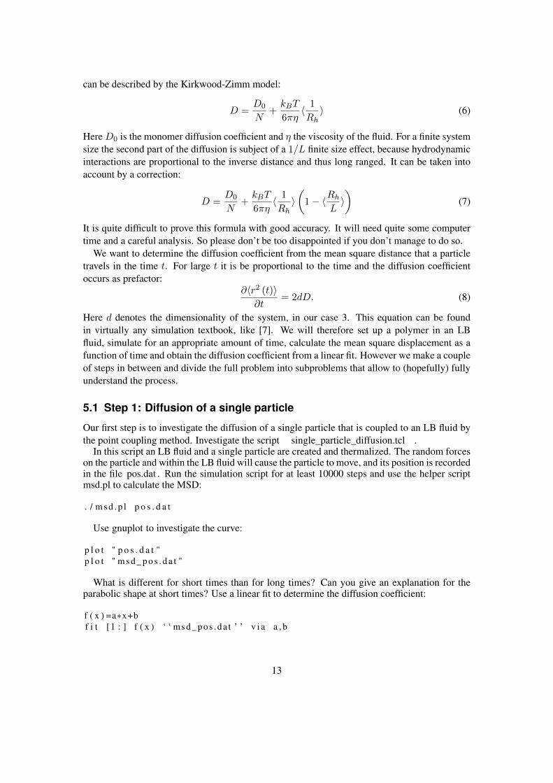
Our first step is to investigate the diffusion of a single particle that is coupled to an LB fluid bythe point coupling method. Investigate the script single_particle_diffusion.tcl .

In this script an LB fluid and a single particle are created and thermalized. The random forceson the particle and within the LB fluid will cause the particle to move, and its position is recordedin the file pos.dat . Run the simulation script for at least 10000 steps and use the helper scriptmsd.pl to calculate the MSD:

. / m s d . p l p o s . d a t

Use gnuplot to investigate the curve:

p l o t " p o s . d a t "p l o t " m s d _ p o s . d a t "

What is different for short times than for long times? Can you give an explanation for theparabolic shape at short times? Use a linear fit to determine the diffusion coefficient:

f ( x ) =a∗x+bf i t [1 : ] f ( x ) ‘ ‘ msd_pos .da t ’ ’ v i a a , b

13

-0.02

0

0.02

0.04

0.06

0.08

0.1

0.12

0.14

0 0.1 0.2 0.3 0.4 0.5 0.6 0.7 0.8 0.9 1

mea

n sq

uare

dis

plac

emen

t in

MD

uni

ts

time in MD units

Mean square displacement

Figure 3: Mean square displacement of a single particle

The square brackets in the fit command tell gnuplot only to use the range right of x = 1 forthe fit.

The file energy.dat contains the kinetic energy of the particle as a function of the elapsedsimulation time. Investigate it, by plotting it with gnuplot. Calculate the average value of thekinetic energy e.g. by fitting a constant function with gnuplot. What value would you expectfrom a working thermostat?

Run the simulation again with different values for the friction coefficient, e.g. 1. 2. 4. 10.Calculate the diffusion coefficient for all cases and use gnuplot to make a plot of D as a functionof γ. What do you observe? The tiny helper script fit_lin.sh (with argument msd_pos.dat)will help you with that. It contains a (quite ugly) gnuplot one-liner that does the fitting and justreturns the slope. The fit is performed in the range 5 to 40 that has proved to work good for runsof ∼ 100000 steps. You have to modify the script to change that range. Is there any differencebetween the friction coefficient that you put in, and the diffusion coefficient you obtain?

5.2 Step 2: Diffusion of a polymer

One of the typical applications of ESPResSo is the simulation of polymer chains with a bead-spring-model. For this we need a repulsive interaction between all beads, for which one usuallytakes a shifted and truncated Lennard-Jones (so called Weeks-Chandler-Anderson) interaction,and additionally a bonded interaction between adjacent beads to hold the polymer together. Youhave already learned that the command

14

i n t e r 0 0 l e n n a r d− j o n e s 1 . 1 . 1 . 1 2 5 0 . 2 5 0 .

creates a Lennard-Jones interaction with ε = 1. σ = 1. rcut = 1.125 and εshift = 0.25between particles of type 0, the desired repulsive interaction. The command

i n t e r 0 FENE 7 . 2 .

creates a FENE (see ESPResSo manual for the details) bond interaction. Still ESPResSo doesnot know between which beads this interaction should be applied. This can be either be specifiedexplicitly or done with the polymer command. This creates a given number of beads, links themwith the given bonded interaction and places them following a certain algorithm. We will usethe pruned self-avoiding walk: The monomers are set according to a pruned self-avoiding walk(in 3D) with a fixed distance between adjacent bead positions. The syntax is:

polymer $N_polymers $N_monomers 1 . 0 t y p e s 0 mode PSAW bond 0

Using a random walk to create a polymer causes trouble: The random walk may cross it-self (or closely approach itself) and the LJ potential is very steep. This would raise the po-tential energy enormously and would make the monomers shoot through the simulation box.The pruned self-avoiding walk should prevent that, but to be sure we perform some MD stepswith a capped LJ potential, this means forces above a certain threshold will be set to the thresh-old in order to prevent the system from exploding. To see how this is done, look at the scriptpolymer_diffusion.tcl . It contains a quite long warmup command so that also longer polymers

are possible. You can probably make it shorter. Also the runtime can be reduced. You shouldfind out about necessary number of steps by yourself.

It is called in the following way:

/ p a t h / t o / E s p r e s s o p o l y m e r _ d i f f u s i o n $N_monomers

This allows to quickly change the number of monomers without editing the script. Changethe variable vmd_output to yes to look at the diffusing polymer. For the warmup a Langevinthermostat is used to keep the temperature constant. You will have to add the LB command byyourself.

Run the script with a polymer of chain length 16 and look at the output files which are identicalto the output files of the single_particle_diffusion.tcl script. Use msd.pl and fit_lin.sh tocalculate the diffusion coefficient as a function of the chain length. If you are familiar withshell scripting, write a script that automatically changes the chain length. Additionally the scriptwrites the file rh.dat that contains the instantaneous value of the hydrodynamic radius. Thescript average.sh allows to calculate its average value.

With the help of the single particle script now add the LB fluid and calculate the MSD again.What do you observe? Do not forget to remove the Langevin thermostat after the warmup. Thiscan be done with the command

thermos ta t o f f

Can you confirm the behaviour of eq. 7 when a LB fluid is added? Not very easy to answeris the question of the statistical accuracy of the data. A good way is to run the same simulation

15

several times so that it produced statistically independent data and then calculate the standarddeviation of the mean, like in lab experiments.

To check the Kirkwood-Zimm formula (eq. 7) we have used shell scripts of the followingtype:

n= " 10 20 30 40 50 60 80 90 100 "f o r i i n $n ; do

mkdir $ icd $ i~ / e s p r e s s o− g i t / e s p r e s s o / b i n / E s p r e s s o . . / p o l y m e r _ d i f f u s i o n . t c l $ icd . .

done

n= " 10 20 30 40 50 60 80 90 100 "f o r i i n $n ; do

cd $ i. . / . . / s r c / m s d . p l p o s . d a t > / dev / n u l l. . / . . / s r c / a c f _ c o l u m n w i s e . p l v . d a t > / dev / n u l la= ‘ . . / . . / s r c / f i t _ l i n . s h msd_pos .da t ‘b= ‘ . . / . . / s r c / a v e r a g e . s h r h . d a t ‘echo " $ i $a $b "cd . .

done

Maybe this is a helpful starting point for you.

6 Electro-osmotic flow in a slit pore

Electro-osmotic flow (EOF) is the motion of water (or another liquid) induced by an electricfield. It can occur e.g. in porous media, in synthetic capillaries and in vicinity of charged sur-faces. Charged objects in an electrolyte solution attract ions of one species and repel ions of theother species, which gives rise to a net charge density in its neighbourhood. If an external elec-tric field is applied, these ions are accelerated in the direction of the electric field (or oppositelyif negatively charged) which causes also an acceleration of the surrounding water. In regionswith zero net charge, the force on the fluid exerted by both ion species cancels, thus chargedinterfaces are necessary.

Conceptually electro-osmotic flow is closely related to electrophoresis, where a charged object(e.g. a polyelectrolyte) is moved by an electric field and the surrounding counterions create aflow field in the opposite direction.

In this exercise the electrokinetic equations, that allow for a classical description of the phe-nomenon, are introduced and you will learn how to simulate this effect with ESPResSo with theLBM. The special case of planar charged walls in the regime of low salt concentration can besolved analytically and you will see that we can reproduce the classical results quite well, butyou will also learn about the deficiencies of both approaches. We will concentrate on the casewhere only one species of ions (counterions) is present. The generalization to multiple specieshowever is straightforward.

16

6.1 The electrokinetic equations

We want to describe a system in which ions can diffuse under an applied field embedded in afluid. We therefore assume that a linear convection diffusion equation is valid:

~j = −D∇ρ− ρ (µze∇Φ + ~u) ,

Here ~j corresponds to the ion flux density, D corresponds to the diffusion coefficient of theions, c to their concentration, µ to their (electrophoretic) mobility, ~E to the local electric fieldand ~u to the fluid velocity.

We assume that fluid fulfills the incompressible Navier-Stokes equation. The term ρze ~Eappears as source term due to the acceleration of the fluid caused by the ions. In the limit ofsmall Reynolds numbers we can leave out the convection term and reduce to the Stokes equation.

η∆~u = ~∇p− ρze ~E (9)

Here we have assumed that the system reaches a steady state and therefore the time derivativewas dropped. The incompressibility (=continuity) equation holds:

~∇ · ~u = 0 (10)

For the electrostatic potential we make the following mean field approximation: The electricpotential is caused not by single ions, but their density. This means every ion is not exposed tothe instantaneous electrostatic potential but the smeared out potential of all other ions. Then thePoisson equation reads as:

∆Φ = −ρze/ε (11)

We will later see that this approximation is avoided in a molecular dynamics simulation ofexplicit ions.

This set of coupled partial differential equations is called the electrokinetic equations. In gen-eral the solution is difficult, but the planar geometry will allow us to find an analytical solution.

6.2 The slit pore geometry

We want to investigate the simplest case where EOF occurs: The flow of water through thevolume between two parallel charged planes in the xy-plane. We assume that the planes areinfinitely extended in the directions parallel to the plane and that the number of ions exactlycancels the charge of both planes and that the external electric field is exerted in x direction andthat the position of the planes is at x = ±l/2.

We assume that all quantities to not change in y and z directions because of translationalinvariance (the great advantage of our geometry) and drop all derivatives with respect to it. Theonly exception is the electrostatic potential which we assume to decay linearly in y-directiondue to an external field.

Due to continuity in x-direction and translational invariance resp. symmetry the fluid velocityand flux density in x direction must be zero and we can write down the Poisson equation and the

17

diffusion equation in x direction:

∂2xΦ = −ρze/ε (12)

0 = −D∂xρ− ρµze∂xΦ (13)

This significantly smaller set of equations corresponds to the 1D Poisson-Boltzmann equation.It can be solved using the Ansatz:

ρ = c exp

(− zeΦkBT

)(14)

Then one obtains a single ordinary differential equation that has to be solved under the boundarycondition that the walls bear a charge density σ, thus electric field jumps at x = ±l/2. Thisyields:

ρ(y) =εC2

2kBT· 1

cos2(

qC2kBT

· y) , ∣∣∣∣ qC

2kBT· y∣∣∣∣ < π

2.

Here the parameter C has to fulfill the following transcendental equation:

C · tan

(qd

4kBT· C)

= −σε, 0 ≤ C <

πkBT

2d|q|.

Now this charge density can be included in the Stokes equation and one can obtain the fluidprofile from integrating twice and choosing the integration constanst so that ~u = 0 is fulfilled atx = ±l/2:

uy(x) =2EεkBT

ηq·{

log

[cos

(qC

2kBT· x)]− log

[cos

(dqC

4kBT

)]},

Obtaining the particle flux profile is the easy:

jy/ρ = µE + uy. (15)

Before simulating the full system, we make two steps in between, because we need to knowhow to have walls in an ESPResSo simulation. First we want to simulate Poisseuille flow,the famous parabolic flow profile, in a slit geometry and then we want to simulation particlesbetween two walls. Finally we combine it all to simulate the full system.

6.3 Poiseuille flow ESPResSo

Poisseuille flow is the flow through a pipe or (in our case) a slit under a homogenous forcedensity, e.g. gravity. In the limit of small Reynolds numbers, the flow can be described with theStokes equation. We assume the slit being infinitely extended in y and z direction and an forcedensity f on the fluid in y direction. No slip-boundary conditions (i.e. ~u = 0) are located at

18

z = ±l/2. Assuming invariance in y and z direction and a steady state the Stokes equation issimplified to:

η∂2xuy = f (16)

where f denotes the force density and η the dynamic viscosity. This can be integrated twice andthe integration constants are chosen so that uy = 0 at z = ±l/2 and we obtain:

uy =f

2η

(l2/4− x2

)(17)

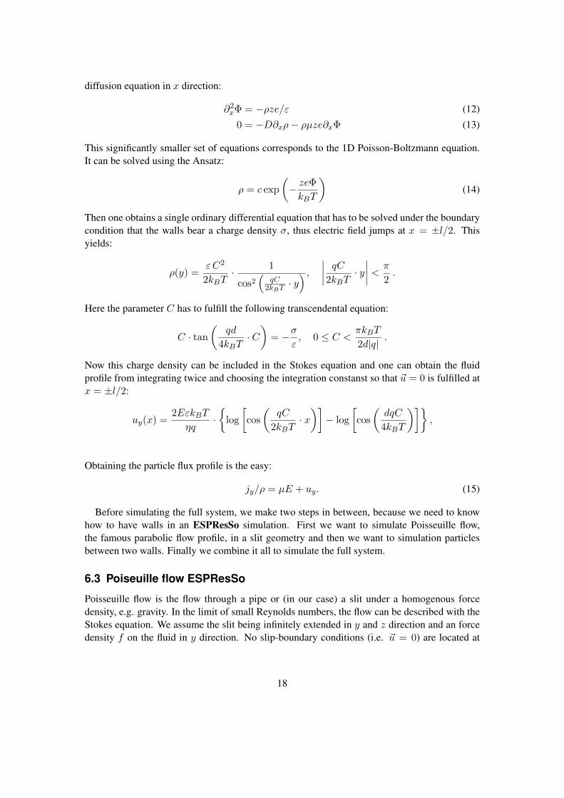
With that knowledge investigate the script poisseuille.tcl. Note the lbboundary command. Twowalls are created with normal vectors (±1, 0, 0). An external force is applied to every node.After 1000 LB updates the steady state should be reached.

Task: Write a loop that prints the fluid velocity at the nodes (0,0,0) to (16,0,0) and the nodeposition to a file. Use the lbnode command for that. Hint: to write to a file, first open a file andthen use the puts command to write into it. Do not forget to close the file afterwards. Example:

s e t o f i l e [ open " f i l e . t x t " "w" ]puts $ o f i l e " h e l l o wor ld ! "c l o s e $ o f i l e

Use gnuplot to fit a parabolic profile. Can you confirm the analytic solution?

-0.01

-0.005

0

0.005

0.01

0.015

0.02

0.025

0 2 4 6 8 10 12 14 16

flui

d ve

loci

ty (

MD

uni

ts)

position in nm

Velocity Profile

Figure 4: Poisseuille Flow in a slit Geometry.

19

6.4 Constraints in ESPResSo

The constraint command of ESPResSo creates walls in the system. They have a particular“particle” type and interact with the particles present in the system with the potential definedbetween them. This means the distance of every particle to the constraint is calculated and usedas the distance in the interaction potential.

To set up a planar channel like the LB channel before one would use the commands:

c o n s t r a i n t w a l l d i s t 0 . 5 normal 1 . 0 . 0 . type 1c o n s t r a i n t w a l l d i s t −8.5 normal −1. 0 . 0 . type 1i n t e r 0 1 l e n n a r d− j o n e s 1 . 1 . 1 . 2 2 5 0 . 2 5 0

This wall is felt only by particles of type 0 and has an effective width of 6, as the potential goessteeply up at positions x = 1.5 and x = 7.5.

The syntax of the wall constraint looks weird at first, because a negative distance from theorigin (first argument) is given, but the idea is that this distance times the normal vector is apoint of the plane. For inclined walls this syntax is more easy to understand.

ESPResSo complains every time a particle penetrates the wall, as it does not expect the par-ticles to do so. This complaint should be taken serious, because that means the particle hasovercome LJ potential barrier, which is physically impossible. This usually tells you to reducethe applied time step.

To set up a system we have, of course to make sure, that our initial configuration obeys theconstraints. The easiest thing is to generate particle particle positions randomly and check ifit obeys the constraint. If not we repeat this process for every particle until a configuration isfound, that is within the allowed range. Look at the script boundaries.tcl and see how that issolved. What does the script do?

6.5 Simulating EOF in ESPResSo

The last thing that is missing for the simulation of EOF is how to create a charged wall. Thiscan be done with particles, using the fix command. The command

part 0 pos 1 . 1 . 1 . q 1 . f i x 1 1 1

create a particle at the position (1, 1, 1) with charge 1 that is fixed in all the spacial dimensions.In eof.tcl two walls are created. Now use the material from the other two scripts to run the

final system. Our we want to obtain a 10 Nanometer wide channel centered x = 7.5

1. Create constraints at x = 1.5 and x = 13.5 and create a particle-wall interaction. Howcan you assure that the particles creating the wall charges are not affected by interactionpotential.

2. Use the particle creation method from boundaries.tcl to create particles in the system.Create a repulsive potential between them.

3. Charge the particles so that the overall system is neutral.

4. Add an electrostatic interaction with a Bjerrum length of 0.7 (the room temperature Bjer-rum length of water in nanometer).

20

5. First do not exert an external force on the particles. Use a Langevin thermostat to bringthe system to equilibrium. It will take some time for the ions to move towards the chargedwalls. You can use vmd to look see the process.

6. Use the density profile method from boundaries.tcl to determine the ion concentrationprofile. How many samples do you need to get a reasonable concentration profile.

7. Plot the concentration profile with gnuplot. Compare with the the Poisson-Boltzmannresult.

8. Introduce an LB fluid with planar walls boundaries at 2.5 and 12.5. Do not forget toremove the external force if you copy&paste from poisseuille.tcl .

9. Add an external force of 0.1 to all particles that do not form the charged wall in y-direction.Now run the system for enough time steps to get a good flux and velocity profile.

10. Finally calculate the velocity profile. You will have to average over several steps. Keepin mind that number crunching with tcl is slow and that you will not need to average overtoo many samples.

11. Compare the flux and velocity profiles with the result from theory. Do they agree?

12. Now increase the charge density on the walls. Can you observe differences between theoryand Computer simulations? They will likely be caused by the fact, that MD simulationsof explicit ions automatically take into account ion correlations and the effect of the finitesize of ions.

Following this list should in principle enable you to simulate the system. However we havefigured out that quite some traps are on the way to the full system. You might have to makewarmup steps in between, play with the time step and so on until your simulation script isreally stable. If something happens, make sure you check all the stages in between, or makesimplifications e.g. disabling the electrostatic interactions. This is however part of the processto learn ESPResSo. If it takes you some time, do not be disappointed, but consider it a part ofyour learning curve.

References

[1] S Succi. The lattice Boltzmann equation for fluid dynamics and beyond. Clarendon Press,Oxford, 2001.

[2] B. Dünweg and A. J. C. Ladd. Advanced Computer Simulation Approaches for Soft MatterSciences III, chapter II, pages 89–166. Springer, 2009.

[3] B. Dünweg, U. Schiller, and A.J.C. Ladd. Statistical mechanics of the fluctuating lattice-boltzmann equation. Phys. Rev. E, 76:36704, 2007.

[4] P. G. de Gennes. Scaling Concepts in Polymer Physics. Cornell University Press, Ithaca,NY, 1979.

21

[5] M. Doi. Introduction do Polymer Physics. Clarendon Press, Oxford, 1996.

[6] Michael Rubinstein and Ralph H. Colby. Polymer Physics. Oxford University Press, Oxford,UK, 2003.

[7] Daan Frenkel and Berend Smit. Understanding Molecular Simulation. Academic Press,San Diego, second edition, 2002.

22