The lattice Boltzmann method as a basis for ocean ...rsalmon/salmon.1999a.pdf · Numerical ocean circulation modelers usually follow one of two strategies. Numerical models based

The lattice Boltzmann method as a basisfor ocean circulation modeling

by Rick Salmon1

ABSTRACTWe construct a lattice Boltzmann model of a single-layer, ‘‘reduced gravity’’ ocean in a square

basin, with shallow water or planetary geostrophic dynamics, and boundary conditions of no slip orno stress. When the volume of the moving upper layer is sufficientlysmall, the motionless lower layeroutcrops over a broad area of the northern wind gyre, and the pattern of separated and isolatedwestern boundary currents agrees with the theory of Veronis (1973). Because planetary geostrophicdynamics omit inertia, lattice Boltzmann solutions of the planetary geostrophic equations do notrequire a lattice with the high degree of symmetry needed to correctly represent the Reynolds stress.This property gives planetary geostrophic dynamics a signi� cant computational advantage over theprimitive equations, especially in three dimensions.

1. Introduction

Numerical ocean circulation modelers usually follow one of two strategies. Numericalmodels based upon the primitive equations represent the � rst strategy. In primitiveequation models, inertia-gravity waves are present even though these waves are unimpor-tant contributors to the large-scale ocean circulation.The presence of inertia-gravity wavesseverely limits the size of the time step in primitive equation models. However, because ofthe inertia-gravity waves, the primitive equations comprise relatively few diagnosticequations and are, therefore, relatively easy to code and solve.

The second strategy employs balanced dynamical equations like the quasi-geostrophicor semi-geostrophic equations. In numerical models based upon balanced dynamics,inertia-gravity waves are absent; therefore, the time step can be much larger. However, theapproximations used to � lter out the inertia-gravity waves require the solution of addi-tional, typically elliptic, and frequently nonlinear diagnostic equations. The in� nitepropagation speed associated with the diagnostic equations is a direct result of the balancecondition that � lters out inertia-gravity waves. In complex geometry, that is, with realisticocean bathymetry, the only practical methods for solving the diagnostic equations areiterative. Unfortunately, iterative solution of the diagnostic equations can be more difficult

1. Scripps Institution of Oceanography, University of California, La Jolla, California, 92093-0225, U.S.A.email: [email protected]

Journal of Marine Research, 57, 503–535, 1999

503

and less efficient than time-stepping the primitive equations, even when the solutionsthemselves are nearly geostrophic.

Lattice Boltzmann methods (hereafter LB) offer a third modeling strategy that, unlikeboth the primitive and balanced dynamical equations, is completely prognostic. Thus LBocean models contain not only inertia-gravity waves but sound waves as well. In fact,because LB models contain an arbitrary number of dependent variables (corresponding tothe arbitrary number of links between neighboring lattice points), LB models typicallycontain more types of waves than are actually present in the dynamical equations ofinterest. These extra modes, which we shall call fast modes, play a role that is closelyanalogous to the role played by inertia-gravity waves in solutions of the primitiveequations. Although unimportant contributors to the whole solution, the fast modes carryinformation rapidly throughout the � ow, removing the need for diagnostic equations of anykind.

Despite the presence of many fast modes, LB methods are efficient because the fastmodes can be made to propagate at speeds which, although much faster than the slowmodes of real physical interest, are very much slower than, for example, the speed of realsound waves. Thus LB methods resemble still another well-known scheme for modelingbalanced dynamics, in which fast modes are not removed but instead simply slowed downby making parameter adjustments to the physics. However, compared to other methods forslowing down fast waves, LB methods, which amount to a technique of slowing andattenuation, seem more sophisticated.

Usually, but perhaps mainly for historical reasons, we regard the LB equations asequations governing the average behavior of an underlying lattice gas. Lattice gases arehighly idealized models of the complete molecular dynamics of real � uids. However,because much of the energy in lattice gases is thermal energy, lattice gases constitute rathernoisy models of macroscopic � uids. A principal advantage of the LB method over thelattice gas method is that LB � lters out this noise. Thus LB models are, in a sense, balancedmodels, which despite their many degrees of freedom and high proportion of fast modes,� lter out the ultra fast modes corresponding to thermal motions.

The great practical advantage of LB models lies in the extraordinary simplicity of the LBequations, their numerical stability, and in the fact that the LB equations are massivelyparallel: At each timestep, the LB solution algorithm proceeds without consulting theconditions at the neighboring lattice points. Thus each lattice point could have its ownprocessor. These practical advantages more than compensate for the extra storage associ-ated with the greater number of dependent variables.

While it is their potential for parallel processing that virtually guarantees that LBmethods will play an important role in ocean circulation modeling, it is their mathematicalsimplicity that seems most appealing.With only slight exaggeration, one could say that theLB method never requires the computation of a derivative. Nevertheless, one can interpretthe LB equations as � nite-difference approximations to a simple and completely hyper-

504 Journal of Marine Research [57, 3

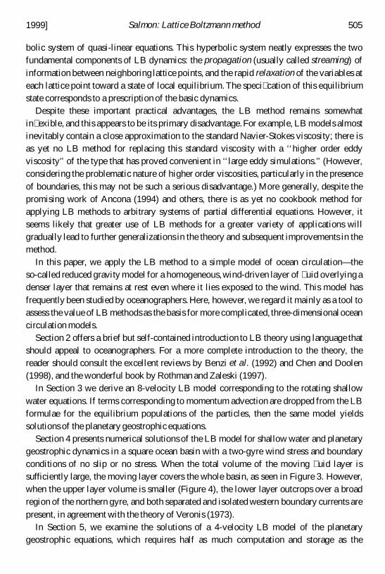
bolic system of quasi-linear equations. This hyperbolic system neatly expresses the twofundamental components of LB dynamics: the propagation (usually called streaming) ofinformation between neighboring lattice points, and the rapid relaxation of the variables ateach lattice point toward a state of local equilibrium. The speci� cation of this equilibriumstate corresponds to a prescription of the basic dynamics.

Despite these important practical advantages, the LB method remains somewhatin� exible, and this appears to be its primary disadvantage.For example, LB models almostinevitably contain a close approximation to the standard Navier-Stokes viscosity; there isas yet no LB method for replacing this standard viscosity with a ‘‘higher order eddyviscosity’’ of the type that has proved convenient in ‘‘large eddy simulations.’’ (However,considering the problematic nature of higher order viscosities, particularly in the presenceof boundaries, this may not be such a serious disadvantage.) More generally, despite thepromising work of Ancona (1994) and others, there is as yet no cookbook method forapplying LB methods to arbitrary systems of partial differential equations. However, itseems likely that greater use of LB methods for a greater variety of applications willgradually lead to further generalizations in the theory and subsequent improvements in themethod.

In this paper, we apply the LB method to a simple model of ocean circulation—theso-called reduced gravity model for a homogeneous,wind-driven layer of � uid overlying adenser layer that remains at rest even where it lies exposed to the wind. This model hasfrequently been studied by oceanographers.Here, however, we regard it mainly as a tool toassess the value of LB methods as the basis for more complicated, three-dimensionaloceancirculation models.

Section 2 offers a brief but self-contained introduction to LB theory using language thatshould appeal to oceanographers. For a more complete introduction to the theory, thereader should consult the excellent reviews by Benzi et al. (1992) and Chen and Doolen(1998), and the wonderful book by Rothman and Zaleski (1997).

In Section 3 we derive an 8-velocity LB model corresponding to the rotating shallowwater equations. If terms corresponding to momentum advection are dropped from the LBformulae for the equilibrium populations of the particles, then the same model yieldssolutions of the planetary geostrophic equations.

Section 4 presents numerical solutions of the LB model for shallow water and planetarygeostrophic dynamics in a square ocean basin with a two-gyre wind stress and boundaryconditions of no slip or no stress. When the total volume of the moving � uid layer issufficiently large, the moving layer covers the whole basin, as seen in Figure 3. However,when the upper layer volume is smaller (Figure 4), the lower layer outcrops over a broadregion of the northern gyre, and both separated and isolated western boundary currents arepresent, in agreement with the theory of Veronis (1973).

In Section 5, we examine the solutions of a 4-velocity LB model of the planetarygeostrophic equations, which requires half as much computation and storage as the

1999] 505Salmon: Lattice Boltzmann method

8-velocity model of Sections 3 and 4. In Sections 5 and 6, we speculate that thethree-dimensional analogue of the 4-velocity model holds great promise as the basis for athree-dimensional global ocean circulation model.

Lattice gas models and LB models have been widely used in � uid mechanics for aboutten years, and several applications treat problems of geophysical � uid dynamics. Forexample, Benzi et al. (1998) present results from a 512-processor LB calculation ofRayleigh-Benard convection on a 2563 lattice. However, I have not seen the LB methodapplied to rotating � ow. Since, therefore, few oceanographers are likely to be familiar withthe LB method, this paper is designed to be as self-contained as possible.

2. The lattice Boltzmann method

We illustrate the lattice Boltzmann method by application to the uni-directional waveequation,

h

t1 cR(h)

h

x5 0, (2.1)

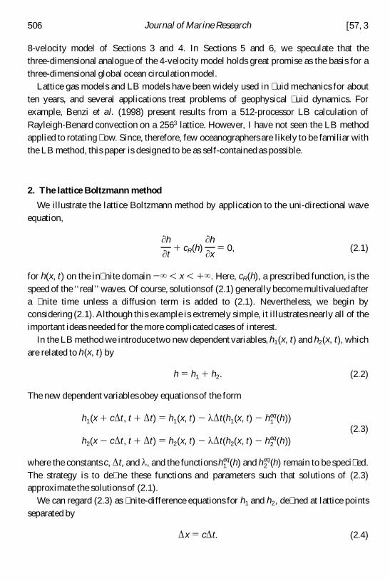
for h(x, t) on the in� nite domain 2 ` , x , 1 ` . Here, cR(h), a prescribed function, is thespeed of the ‘‘real’’waves. Of course, solutionsof (2.1) generally become multivaluedaftera � nite time unless a diffusion term is added to (2.1). Nevertheless, we begin byconsidering (2.1). Although this example is extremely simple, it illustrates nearly all of theimportant ideas needed for the more complicated cases of interest.

In the LB method we introduce two new dependent variables, h1(x, t) and h2(x, t), whichare related to h(x, t) by

h 5 h1 1 h2. (2.2)

The new dependent variables obey equations of the form

h1(x 1 c D t, t 1 D t) 5 h1(x, t) 2 l D t(h1(x, t) 2 h1eq(h))

h2(x 2 c D t, t 1 D t) 5 h2(x, t) 2 l D t(h2(x, t) 2 h2eq(h))

(2.3)

where the constants c, D t, and l , and the functions h1eq(h) and h2

eq(h) remain to be speci� ed.The strategy is to de� ne these functions and parameters such that solutions of (2.3)approximate the solutions of (2.1).

We can regard (2.3) as � nite-difference equations for h1 and h2, de� ned at lattice pointsseparated by

D x 5 cD t. (2.4)


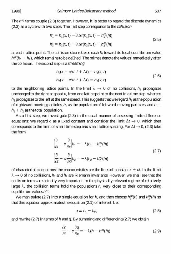
The heq terms couple (2.3) together. However, it is better to regard the discrete dynamics(2.3) as a cycle with two steps. The � rst step corresponds to the collision

h81 5 h1(x, t) 2 l D t(h1(x, t) 2 h1eq(h))

h82 5 h2(x, t) 2 l D t(h2(x, t) 2 h2eq(h))

(2.5)

at each lattice point. The collision step relaxes each hi toward its local equilibrium valueh i

eq(h1 1 h2), which remains to be de� ned. The primes denote the values immediately afterthe collision.The second step is a streaming

h1(x 1 cD t, t 1 D t) 5 h81(x, t)

h2(x 2 cD t, t 1 D t) 5 h82(x, t)(2.6)

to the neighboring lattice points. In the limit l ® 0 of no collisions, h1 propagatesunchanged to the right at speed c, from one lattice point to the next in a time step, whereash2 propagates to the left at the same speed. This suggests that we regard h1 as the populationof rightward-moving particles, h2 as the population of leftward-moving particles, and h 5h1 1 h2 as the total population.

As a � rst step, we investigate (2.3) in the usual manner of assessing � nite-differenceequations: We regard c as a � xed constant and consider the limit D t ® 0, which thencorresponds to the limit of small time step and small lattice spacing. For D t ® 0, (2.3) takethe form

1 t1 c

x 2 h1 5 2 l (h1 2 h1eq(h))

1 t2 c

x 2 h2 5 2 l (h2 2 h2eq(h))

(2.7)

of characteristic equations; the characteristics are the lines of constant x 6 ct. In the limitl ® 0 of no collisions, h1 and h2 are Riemann invariants. However, we shall see that thecollision terms are actually very important. In the physically relevant regime of relativelylarge l , the collision terms hold the populations hi very close to their correspondingequilibrium values h i

eq.We manipulate (2.7) into a single equation for h, and then choose h1

eq(h) and h2eq(h) so

that this equation approximates the equation (2.1) of interest. Let

q ; h1 2 h2, (2.8)

and rewrite (2.7) in terms of h and q. By summing and differencing (2.7) we obtain

h

t1 c

q

x5 2 l (h 2 heq(h)) (2.9)


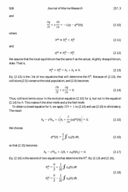
and

q

t1 c

h

x5 2 l (q 2 qeq(h)) (2.10)

where

heq ; h1eq 1 h2

eq (2.11)

and

qeq ; h1eq 2 h2

eq. (2.12)

We assume that the local equilibrium has the same h as the actual, slightly disequilibrium,state. That is,

h1eq 1 h2

eq 5 h1 1 h2 ; h. (2.13)

Eq. (2.13) is the � rst of two equations that will determine the h ieq. Because of (2.13), the

collisions (2.5) conserve the total population, and (2.9) becomes

h

t1 c

q

x5 0. (2.14)

Thus, collision terms occur in the evolution equation (2.10) for q, but not in the equation(2.14) for h. This makes h the slow mode and q the fast mode.

To obtain a closed equation for h, we apply / t 1 l to (2.14) and use (2.10) to eliminate q.The result

htt 2 c2hxx 1 l 1 ht 1

x(cqeq(h)) 2 5 0. (2.15)

We choose

qeq(h) 51

ce cR(h) dh, (2.16)

so that (2.15) becomes

htt 2 c2hxx 1 l (ht 1 cR(h)hx) 5 0. (2.17)

Eq. (2.16) is the second of two equations that determine the h ieq. By (2.13) and (2.16),

h1eq 5

h

21

1

2c e cR(h) dh

h2eq 5

h

22

1

2ce cR(h) dh.

(2.18)


If we take the lattice spacing D x as given, then, by (2.4), the choice of c corresponds to thechoice of time step D t. Thus the LB dynamics (2.3) is completely speci� ed by (2.18) andthe choice of c and l .

Eq. (2.17) represents the sum of the ‘‘textbook’’ wave equation, with propagation speedc, plus l multiplied by the equation (2.1) of interest. Therefore we should choose l largeenough so that the last two terms in (2.17) dominate the � rst two terms. The second term in(2.17) is a diffusion term of the kind required to keep (2.1) well behaved. On the otherhand, the � rst term in (2.17) is unphysical, from the standpoint of (2.1). In summary then,our strategy should be to choose l and c such that

* htt * ½ * c2hxx * ½ * l cRhx * . (2.19)

Then, neglecting only the smallest term, (2.17) becomes

ht 1 cR(h)hx 5c2

lhxx, (2.20)

the diffusive form of (2.1). From (2.20), we see that for � xed D x and D t, and hence � xed c,l controls the diffusion coefficient c2/l .

Suppose that cR(h) is nearly uniform, either because h is nearly uniform, or becausecR(h) is a nearly constant function. Then since ht < cRhx, we have htt < cR

2hxx, and the � rstinequality in (2.19) corresponds to

cR , c. (2.21)

By (2.4), this is just the usual CLF criterion,

cR ,D x

D t, (2.22)

that the physical wave cannot propagate farther than a lattice distance D x in a time step D t.If we include the effects of the � rst term in (2.17) (still assuming ht < cRhx), then (2.20)becomes

ht 1 cR(h)hx 5c2 2 cR

2

lhxx. (2.23)

Thus, violation of the CLF criterion leads to instability in the form of a negative diffusionin (2.23).

The present example is an especially simple one. In more complicated cases, particularlythose involving more than one space dimension, such a direct analysis of the full set ofpopulation equations becomes impractical. In these cases, it is better to use an approxima-tion method—the Chapman-Enskog expansion—that explicitly tracks only the slowmodes. Because it treats the more numerous fast modes only implicitly, the Chapman-


Enskog expansion can be carried to a higher order in D t. This higher accuracy is important.For example, (2.20) suggests that the diffusion can be made arbitrarily small by making larbitrarily large, whereas general experience with equations like (2.3) leads us to expectthat l cannot be made much larger than about D t 2 1. Using the more accurate result of theChapman-Enskog expansion, we � nd that the diffusion can indeed be made arbitrarilysmall, but by making l close to the well-de� ned upper bound 2/ D t. This insight provescritical for applications.

The Chapman-Enskog expansion is a dual expansion in D t and in the nearness of each hi

to h ieq. The populations remain near their local equilibrium values because the decay

parameter l is large. Thus e ; 1/ l is the second small parameter. We assume that D t and ehave the same small size, and we take the h i

eq to be given by (2.18). Expanding (2.3) in D t,we obtain

(Di 1 1�2D tDi2 1 · · ·)hi 5 2 l (hi 2 h i

eq), i 5 1, 2 (2.24)

where

D1 5

t1 c

xand D2 5

t2 c

x. (2.25)

Then, expanding the hi about their prescribed equilibrium values,

hi 5 h ieq 1 e h i

(1) 1 e 2h i(2) 1 · · · , e ; l 2 1, (2.26)

and substituting (2.26) into (2.24), we obtain

1 Di 11

2D tDi

2 1 · · · 2 (h ieq 1 e hi

(1) 1 · · ·) 5 21

e( e hi

(1) 1 e 2h i(2) 1 · · ·). (2.27)

To the � rst two orders in D t or e , (2.27) takes the form

G i(0) 1 G i

(1) 5 0, (2.28)

where

G i(0) 5 Dih i

eq 1 h i(1) (2.29)

contains all the order one terms and

G i(1) 5 1�2 D tDi

2hieq 1 e Dih i

(1) 1 e hi(2) (2.30)

contains all the terms of order D t or e .To get a closed equation for the slow mode h(x, t), we sum (2.28) over i and use the

conservation property (2.13) of (2.18), which implies that

oi

h i(1) 5 o

ih i

(2) 5 · · · 5 0. (2.31)


Thus, by (2.18),

oi

G i(0) 5 o

iDih i

eq 5 h

t1 cR(h)

h

x. (2.32)

Similarly,

oi

G i(1) 5

1

2D t o

i

D i2h i

eq 1 e oi

Dih i(1). (2.33)

To consistent order, we may simplify (2.33) by substituting for h i(1) from the leading order

approximation to (2.28), namely

h i(1) 5 2 Dih i

eq. (2.34)

Thus, to consistent order,

oi

G i(1) 5

1

2D t o

iD i

2h ieq 2 e o

iDi(Dihi

eq) 5 1 D t

22

1

l 2 oi

D i2h i

eq. (2.35)

Using (2.18) again, and the fact that ht 5 2 cRhx at leading order, we � nd that, to consistentorder,

oi

D i2hi

eq 5 htt 1 2(cRhx)t 1 c2hxx < (c2 2 cR2 )hxx . (2.36)

Thus, to the � rst two orders in D t and e , the Chapman-Enskog expansion yields

ht 1 cR(h)hx 5 1 1l 2D t

2 2 (c2 2 cR2 )hxx, (2.37)

a more accurate version of (2.23). Once again, if c is much larger than cR, then (2.37)becomes

ht 1 cR(h)hx 5 1 1l 2D t

2 2 c2hxx. (2.38)

Compare (2.38) to the corresponding but less accurate result (2.20). According to (2.38),the diffusion coefficient decreases with increasing l , vanishing as l approaches the criticalvalue 2/D t. For still larger l , the solutions of the LB equations become unstable.

3. The shallow-water equations

In this section we derive the LB approximation to the shallow water equations,

h

t1

xa(u a h) 5 0 (3.1)


and

t(ua h) 1

xbPa b 5 Fa , (3.2)

where

P a b 5 1�2gh2d a b 1 u a ub h. (3.3)

Here, h is the � uid depth, (u1, u2) ; (u, v) ; u is the � uid velocity,g is the gravity constant,and F a is the sum of all the forces including Coriolis force. Repeated Greek subscripts aresummed from 1 to 2.

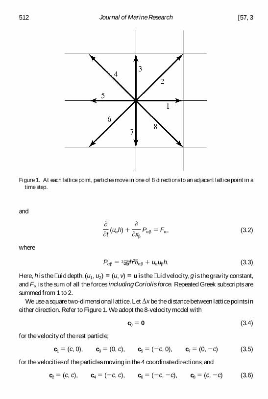
We use a square two-dimensional lattice. Let D x be the distance between lattice points ineither direction. Refer to Figure 1. We adopt the 8-velocity model with

c0 5 0 (3.4)

for the velocity of the rest particle;

c1 5 (c, 0), c3 5 (0, c), c5 5 ( 2 c, 0), c7 5 (0, 2 c) (3.5)

for the velocities of the particles moving in the 4 coordinate directions; and

c2 5 (c, c), c4 5 ( 2 c, c), c6 5 ( 2 c, 2 c), c8 5 (c, 2 c) (3.6)

Figure 1. At each lattice point, particles move in one of 8 directions to an adjacent lattice point in atime step.


for the particle velocities in the 4 diagonal directions. We take cD t 5 D x, so that all theparticles (except the rest particle) move from lattice point to adjacent lattice point in atimestep D t.

As in Section 2, we regard hi(x, t) as the populationof particles with velocity ci at latticepoint x and time t. The equations

h(x, t) 5 oi5 0

8

hi(x, t) (3.7)

and

hu(x, t) 5 oi 5 0

8

cihi(x, t) (3.8)

relate the 9 populations 5 hi(x, t), i 5 0, 86 at lattice point x and time t to the � uid depthh(x, t) and velocity u(x, t) at the same location and time. Since c0 5 0, the rest particles donot contribute to the momentum. The three physical variables h, u, and v are the slowmodes of the LB model. Thus there are 9 2 3 5 6 fast modes.

Once again, the LB dynamics comprises two steps: a collision step, which adjusts thepopulations at each lattice point, followed by a streaming step, in which particles move tothe neighboring lattice points. The collision step is governed by

h8i(x, t) 5 hi(x, t) 2 l D t(hi(x, t) 2 h ieq(x, t)) (3.9)

where l is the decay coefficient, and the prime denotes the value immediately after thecollision.The equilibrium populations

heq(x) ; 5 h0eq(x), h1

eq(x), . . . , h8eq(x) 6 (3.10)

remain to be de� ned. The streaming step is governed by

hi(x 1 ciD t, t 1 D t) 1 h8i(x, t) 1D t

6c2cia 1 12 Fa (x, t) 1

1

2Fa (x 1 ci D t, t 1 D t) 2 (3.11)

where ci a is the component of ci in the a -direction. Once again, repeated Greek indices aresummed. Note that the forcing term in (3.11) represents an average of the values at thedeparture point (x, t) and the arrival point (x 1 ciD t, t 1 D t) of the streaming particle; thisproves essential to maintaining second order accuracy in the Chapman-Enskog expansion.Combining (3.9) and (3.11) into a single formula, we obtain the complete LB dynamics

hi(x 1 ci D t, t 1 D t) 2 hi(x, t) 2D t

6c2cia 1 12 F a (x, t) 1

1

2Fa (x 1 ci D t, t 1 D t) 2

5 2 l D t(hi(x, t) 2 h ieq(x, t)).

(3.12)

Once again, our strategy is to choose the constants c, D t, and l , and the 9 functions


h ieq(h, u, v) (where h, u, v are de� ned by (3.6–8)) such that the slow modes computed from

(3.12) approximately satisfy the shallow water equations.The choices

h0eq 5 h 2

5gh2

6c22

2h

3c2u · u (3.13)

h ieq 5

gh2

6c21

h

3c2ci a ua 1

h

2c4ci a cib u a u b 2

h

6c2u · u, odd i (3.14)

h ieq 5

gh2

24c21

h

12c2cia ua 1

h

8c4ci a cib ua u b 2

h

24c2u · u, even i (3.15)

have the important properties that

oi

h ieq 5 h, (3.16)

oi

ci a h ieq 5 hu a , (3.17)

and

oi

cia ci b h ieq 5

1

2gh2d a b 1 ua u b h. (3.18)

As always, the equilibrium populationsh ieq depend only on the slow modes h, u, and v. The

speci� c choices (3.13–15) are somewhat arbitrary, but we shall see that the properties(3.16–18) guarantee that the slow mode dynamics approximates the shallow-water equa-tions (3.1–3). The properties (3.16) and (3.17) correspond to the conservation of mass andmomentum, respectively, by the collisions (3.9). Property (3.18) makes the momentum � uxof the LB particles equal to the momentum � ux (3.3) of the shallow water equations. For amotivated derivation of (3.13–15), see the Appendix.

The LB dynamics (3.12) comprises 9 evolution equations for the 9 population variableshi. Because there are so many dependent variables, a direct analysis of the full set ofequations like that performed in Section 2 is rather difficult. However, most of thedependent variables represent fast modes. Therefore, the Chapman-Enskog expansion,which pursues only the slow modes, remains relatively easy. Once again, the Chapman-Enskog expansion is a dual expansion in D t and e ; l 2 1, which are assumed to be of thesame order. The smallness of D t (for � xed c) corresponds to the assumption that thepopulation variables vary slowly on the scale of the lattice spacing and the time step. Thesmallness of e corresponds to the assumption that the collisions hold the populations neartheir equilibrium values (3.13–15). Expanding (3.12) in D t, and substituting

hi 5 h ieq 1 e h i

(1) 1 e 2h i(2) 1 · · · (3.19)


we obtain

1 Di 11

2D t Di

2 1 · · ·2 (h ieq 1 e h i

(1) 1 · · ·) 21

6c2cia 1 1 1

1

2D t Di 1 · · ·2 F a (x, t)

5 21

e( e h i

(1) 1 e 2h i(2) 1 · · ·)

(3.20)

where

Di ;

t1 cia

xa. (3.21)

To the � rst two orders in e or D t, (3.20) is

G i(0) 1 G i

(1) 5 0, (3.22)

where

G i(0) 5 Dih i

eq 21

6c2cia Fa 1 h i

(1) (3.23)

contains the order one terms, and

G i(1) 5

1

2D tD i

2h ieq 1 e Dih i

(1) 2D t

12c2ci a DiFa 1 e h i

(2) (3.24)

contains the terms of order D t or e . As in Section 2, we may consistently use the leadingorder balance in (3.22) to simplify the next order terms. Thus solving G i

(0) 5 0 for Dihieq and

substituting the result into (3.24) yields

G i(1) < 1 e 2

D t

2 2 Dih i(1) 1 e hi

(2). (3.25)

To obtain the slow mode dynamics, we apply Siand S

icia to (3.22). Since the heq de� ned

by (3.13–15) satisfy (3.16) and (3.17), it follows from (3.19) that

oi

h i(1) 5 o

i

h i(2) 5 o

i

ci a h i(1) 5 o

i

ci a h i(2) 5 0. (3.26)

Therefore (3.23) implies that

oi

G i(0) 5 o

iDih i

eq 5 h

t1

xa(hu a ), (3.27)

and (3.25) implies that

oi

G i(1) 5 0. (3.28)


Thus the LB dynamics implies the shallow water continuity equation (3.1) with an acuracyof O( e 2).

To obtain the corresponding momentum equation,we use (3.23), (3.26) and (3.16–18) tocompute

oi

ci a G i(0) 5

t(u a h) 1

x bPa b 2 F a , (3.29)

where Pa b is given by (3.3). Similarly, from (3.25) we obtain

oi

ci a G i(1) 5 1 e 2

D t

2 2

x bo

i

cia ci b h i(1). (3.30)

Thus, with an accuracy of O( e 2), the LB dynamics implies

t(u a h) 1

xbPa b 2 Fa 5 2

xbT a b (3.31)

where the viscous tensor

T a b 5 1 e 2D t

2 2 oi

cia ci b h i(1) (3.32)

represents the higher order terms. To consistent order, we may substitute the leading orderbalance

h i(1) 5 2 Dih i

eq 11

6c2cia Fa (3.33)

into the higher order term (3.32). We obtain

T a b 5 1 D t

22 e 2 1

t o i

ci a cib h ieq 1

x go

i

cia ci b cig h ieq 2 . (3.34)

If we choose c2 ¾ gh—the analog of c ¾ cR in Section 2—then the contribution of the / t-term in (3.34) is negligible. Using (3.14–15) to evaluate the other term, we obtain

T a b 5 1 D t

22 e 2 1

3c2 5 = · (hu)d a b 1

x a(hub ) 1

xb(hu a ) 6 . (3.35)

Thus

T a b

x b5 1 D t

22 e 2 1

3c2 5 2

xa= · (hu) 1

2

xb x b(hua ) 6 . (3.36)


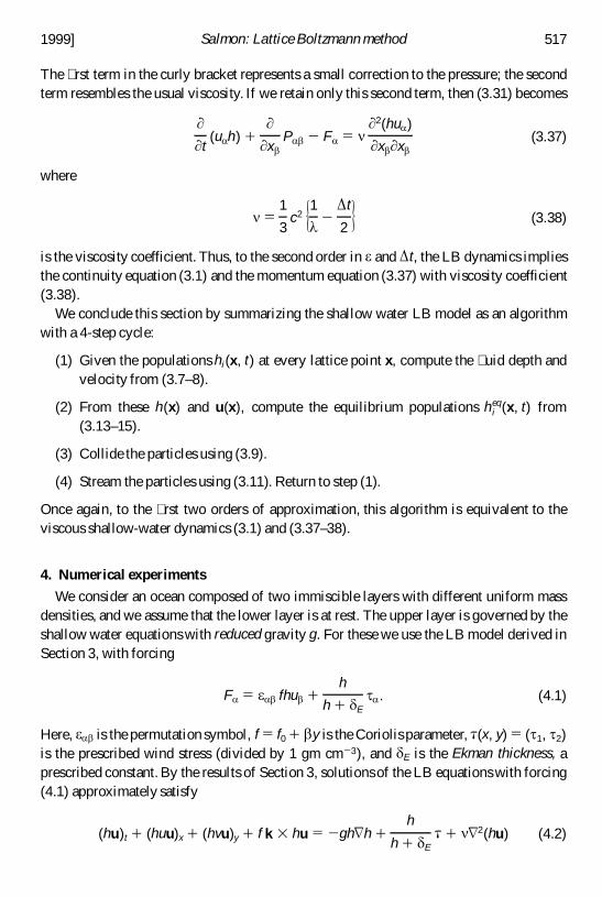
The � rst term in the curly bracket represents a small correction to the pressure; the secondterm resembles the usual viscosity. If we retain only this second term, then (3.31) becomes

t(u a h) 1

x bP a b 2 F a 5 n

2(hu a )

xb xb(3.37)

where

n 51

3c2 5 1l 2

D t

2 6 (3.38)

is the viscosity coefficient. Thus, to the second order in e and D t, the LB dynamics impliesthe continuity equation (3.1) and the momentum equation (3.37) with viscosity coefficient(3.38).

We conclude this section by summarizing the shallow water LB model as an algorithmwith a 4-step cycle:

(1) Given the populations hi(x, t) at every lattice point x, compute the � uid depth andvelocity from (3.7–8).

(2) From these h(x) and u(x), compute the equilibrium populations h ieq(x, t) from

(3.13–15).

(3) Collide the particles using (3.9).

(4) Stream the particles using (3.11). Return to step (1).

Once again, to the � rst two orders of approximation, this algorithm is equivalent to theviscous shallow-water dynamics (3.1) and (3.37–38).

4. Numerical experiments

We consider an ocean composed of two immiscible layers with different uniform massdensities, and we assume that the lower layer is at rest. The upper layer is governed by theshallow water equations with reduced gravity g. For these we use the LB model derived inSection 3, with forcing

Fa 5 e a b fhub 1h

h 1 d Et a . (4.1)

Here, e a b is the permutation symbol, f 5 f0 1 b y is the Coriolis parameter, t (x, y) 5 ( t 1, t 2)is the prescribed wind stress (divided by 1 gm cm 2 3), and d E is the Ekman thickness, aprescribed constant. By the results of Section 3, solutions of the LB equations with forcing(4.1) approximately satisfy

(hu)t 1 (huu)x 1 (hvu)y 1 f k 3 hu 5 2 gh = h 1h

h 1 d Et 1 n = 2(hu) (4.2)


and

h

t1 = · (hu) 5 0, (4.3)

where = 5 ( x, y) and

n 5 1 1l 21

l max2 c2

3, (4.4)

with l max 5 2/ D t and c 5 D x/ D t as before.Models like (4.2–3), often called one-and-one-half layer models or reduced gravity

models, are frequently studied prototypes for the more complex multi-layer or continu-ously strati� ed ocean circulation models. The atypical features of (4.2) are the quotientpreceding the wind stress, and the presence, inside the viscous Laplacian, of the factor h.The latter is a typical feature of LB calculations, an example of the ‘‘in� exibility’’mentioned in Section 1. If u varies on a smaller lengthscale than h, then the viscosity in(4.2) is practically the same as standard Navier-Stokes viscosity. However, in the presentapplication, there is no compelling reason to prefer one form of viscosity over the other. Itis even conceivable that the dissipation operator in (4.2), which arises naturally from thecollide-and-stream algorithm, may have advantages over more arbitrarily chosen dissipa-tion operators. Of course, one could turn off the viscosity in (4.2) by setting l 5 l max, andthen insert a completely arbitrary dissipation into the forcing Fa . However, that wouldviolate the aesthetic principle that LB dynamics should be based on the simplest feasibleset of operations.

As for the quotient in the wind forcing term, we imagine that all of the momentum put inby the wind stress is mixed downward through an ‘‘Ekman layer’’ of depth d E bysmall-scale processes not contained in the model. If the upper layer depth h is much greaterthan d E, then the quotient in (4.1) is near unity, and the upper layer absorbs nearly all of themomentum put in by the wind. However, if h , d E then the upper layer absorbs only afraction, h/d E, of the wind momentum; the rest is lost to the lower layer, which neverthelessremains at rest because of its great presumed thickness. This forcing strategy, which can beviewed as an alternative to interfacial friction, avoids the unrealistic behavior that coulddevelop if a � nite amount of wind mometum were spread over a vanishing upper layerdepth. In all the solutions discussed, d E 5 100 m.

We solve (4.2–3) in the square box, 0 , x, y , L 5 4000 km. All the solutions discussedhave 100 lattice points in each direction. Thus D x 5 40 km. The reduced gravity has thevalue g 5 .002 3 9.8 m sec 2 2. For an upper layer depth of h 5 500 m, this corresponds toan internal gravity wave speed (gh)1/2 of 270 km day2 1. We choose c 5 540 km day2 1 toful� ll the CLF criterion that c be larger than the speed of the gravity waves, the fastestwaves present in the shallow water equations. Then D t 5 D x/c 5 .075 day. We take f0 52 p day2 1 and b 5 f0/6400 km. For h 5 500 m, this corresponds to an internal deformation


radius (gh)1/2/f0 of 43 km, and an internal Rossby wave speed gh b / f 02 of 1.8 km day2 1, at

the southern boundary.At this speed, Rossy waves cross the basin in about 6 years.In all the experiments discussed, t y 5 0, and

t x 5 sin2 ( p y/L) dyn cm2 2. (4.5)

Thus the wind blows west to east with a maximum force at mid-latitude, and both the windstress and its curl vanish at the northern and southern boundaries. The anticipatedcirculation has two gyres.

The relaxation coefficient l controls the viscosity n . Since l is of order D t 2 1, theviscosity n has scale size c2 D t 5 cD x 5 25 3 108 cm2 sec2 1. This corresponds to a Munkboundary layer thickness d M ; ( n / b )1/3 of 280 km, which is too large. Realistically smallviscosity relies on the cancellation between terms in (4.4) as l ® l max. In all of theexperiments discussed, l 5 0.95 3 l max corresponding to v 5 0.033 c D x and d M 5 90 km,about 2 lattice spacings.The ability to reduce the viscosity by choosing l very close to l max

is absolutely vital for the practical application of LB methods. Otherwise the high intrinsicviscosity of LB dynamics makes the solutions unrealistically diffusive. Recall that thel max-term in (4.4) arises from a second order term in D t in the Chapman-Enskogexpansion.

The streaming step (3.11) requires the forcing Fa (x 1 ci D t, t 1 D t) at the particledestination and the new time. Since the forcing (4.1) involves the depth and velocity(which depend on the hi), (3.11) is an implicit equation for hi at the new time. We solve(3.11) using a predictor-corrector method. In the predictor, we evaluate both forcing termsin (3.11) at the departure location and time. In each corrector, we evaluate the forcing termat the destination by using the previous iterate. Although 1 or 2 correctors seemedsufficient, all the solutions discussed use 4 correctors. The need for a predictor/correctormethod to accommodate the Coriolis force somewhat compromises the efficiency andaesthetics of the LB model.

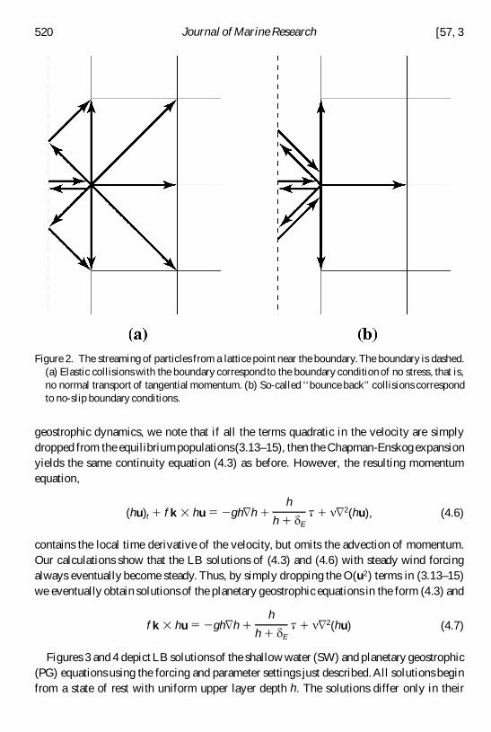
We consider all of the lattice points to lie within the � uid. The collision step is the sameat all lattice points. At the lattice points closest to the boundary, we modify the streamingstep (3.11) to incorporate the boundary conditions.All the experiments discussed used oneof two algorithms. In the algorithm corresponding to no stress, particles streaming towardthe boundary experience elastic collisions, as shown in Figure 2a. In the algorithmcorresponding to no slip, particles streaming toward the boundary bounce back in thedirection from which they came, as shown in Figure 2b. Both of these algorithms arestandard methodology in applications of LB dynamics. Note that, in both cases, theboundary lies one half lattice distance outside the last row of lattice points.Apart from theinteraction with the boundary (that is, as regards the evaluation of the forcing terms and theuse of predictor-corrector), the streaming step is the same at all lattice points.

Parsons (1969) and especially Veronis (1973, 1980) developed a relatively completetheory of wind-driven, reduced-gravity � ow based upon planetary geostrophic dynamics,in which the inertia Du/Dt is omitted from the shallow water momentum equation. For abrief summary of their theory, see Salmon (1998a, pp. 182–188). To investigate planetary


geostrophic dynamics, we note that if all the terms quadratic in the velocity are simplydropped from the equilibrium populations(3.13–15), then the Chapman-Enskog expansionyields the same continuity equation (4.3) as before. However, the resulting momentumequation,

(hu)t 1 f k 3 hu 5 2 gh= h 1h

h 1 d Et 1 n = 2(hu), (4.6)

contains the local time derivative of the velocity, but omits the advection of momentum.Our calculations show that the LB solutions of (4.3) and (4.6) with steady wind forcingalways eventually become steady. Thus, by simply dropping the O(u2) terms in (3.13–15)we eventually obtain solutions of the planetary geostrophic equations in the form (4.3) and

f k 3 hu 5 2 gh= h 1h

h 1 d Et 1 n = 2(hu) (4.7)

Figures 3 and 4 depict LB solutions of the shallow water (SW) and planetary geostrophic(PG) equations using the forcing and parameter settings just described.All solutions beginfrom a state of rest with uniform upper layer depth h. The solutions differ only in their

Figure 2. The streaming of particles from a lattice point near the boundary.The boundary is dashed.(a) Elastic collisions with the boundary correspond to the boundary condition of no stress, that is,no normal transport of tangential momentum. (b) So-called ‘‘bounce back’’ collisions correspondto no-slip boundary conditions.


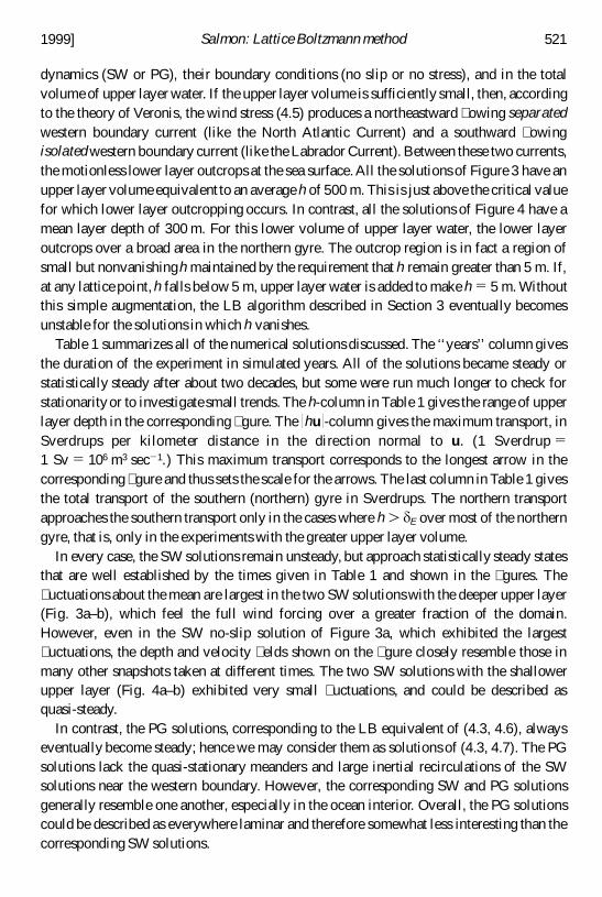
dynamics (SW or PG), their boundary conditions (no slip or no stress), and in the totalvolume of upper layer water. If the upper layer volume is sufficiently small, then, accordingto the theory of Veronis, the wind stress (4.5) produces a northeastward � owing separatedwestern boundary current (like the North Atlantic Current) and a southward � owingisolated western boundary current (like the Labrador Current). Between these two currents,the motionless lower layer outcrops at the sea surface. All the solutions of Figure 3 have anupper layer volume equivalent to an average h of 500 m. This is just above the critical valuefor which lower layer outcropping occurs. In contrast, all the solutions of Figure 4 have amean layer depth of 300 m. For this lower volume of upper layer water, the lower layeroutcrops over a broad area in the northern gyre. The outcrop region is in fact a region ofsmall but nonvanishingh maintained by the requirement that h remain greater than 5 m. If,at any lattice point, h falls below 5 m, upper layer water is added to make h 5 5 m. Withoutthis simple augmentation, the LB algorithm described in Section 3 eventually becomesunstable for the solutions in which h vanishes.

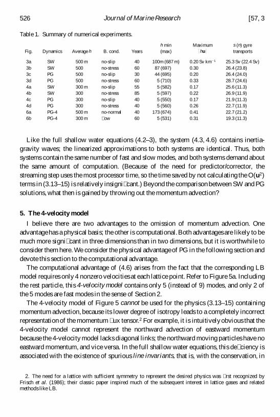
Table 1 summarizes all of the numerical solutions discussed. The ‘‘years’’ column givesthe duration of the experiment in simulated years. All of the solutions became steady orstatistically steady after about two decades, but some were run much longer to check forstationarity or to investigate small trends. The h-column in Table 1 gives the range of upperlayer depth in the corresponding � gure. The * hu * -column gives the maximum transport, inSverdrups per kilometer distance in the direction normal to u. (1 Sverdrup 51 Sv 5 106 m3 sec2 1.) This maximum transport corresponds to the longest arrow in thecorresponding � gure and thus sets the scale for the arrows. The last column in Table 1 givesthe total transport of the southern (northern) gyre in Sverdrups. The northern transportapproaches the southern transport only in the cases where h . d E over most of the northerngyre, that is, only in the experiments with the greater upper layer volume.

In every case, the SW solutions remain unsteady, but approach statistically steady statesthat are well established by the times given in Table 1 and shown in the � gures. The� uctuations about the mean are largest in the two SW solutions with the deeper upper layer(Fig. 3a–b), which feel the full wind forcing over a greater fraction of the domain.However, even in the SW no-slip solution of Figure 3a, which exhibited the largest� uctuations, the depth and velocity � elds shown on the � gure closely resemble those inmany other snapshots taken at different times. The two SW solutions with the shallowerupper layer (Fig. 4a–b) exhibited very small � uctuations, and could be described asquasi-steady.

In contrast, the PG solutions, corresponding to the LB equivalent of (4.3, 4.6), alwayseventually become steady; hence we may consider them as solutions of (4.3, 4.7). The PGsolutions lack the quasi-stationary meanders and large inertial recirculations of the SWsolutions near the western boundary. However, the corresponding SW and PG solutionsgenerally resemble one another, especially in the ocean interior. Overall, the PG solutionscould be described as everywhere laminar and therefore somewhat less interesting than thecorresponding SW solutions.


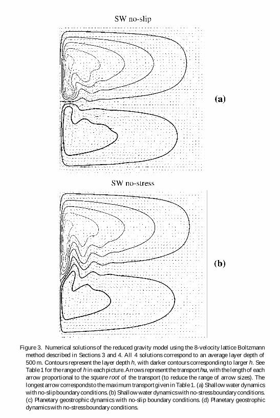
Figure 3. Numerical solutions of the reduced gravity model using the 8-velocity lattice Boltzmannmethod described in Sections 3 and 4. All 4 solutions correspond to an average layer depth of500 m. Contours represent the layer depth h, with darker contours corresponding to larger h. SeeTable 1 for the range of h in each picture.Arrows represent the transporthu, with the length of eacharrow proportional to the square root of the transport (to reduce the range of arrow sizes). Thelongest arrow correspondsto the maximum transportgiven in Table 1. (a) Shallow water dynamicswith no-slip boundary conditions.(b) Shallow water dynamics with no-stress boundaryconditions.(c) Planetary geostrophic dynamics with no-slip boundary conditions. (d) Planetary geostrophicdynamics with no-stress boundary conditions.

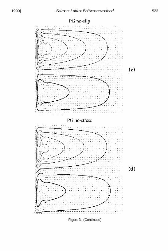
Figure 3. (Continued)


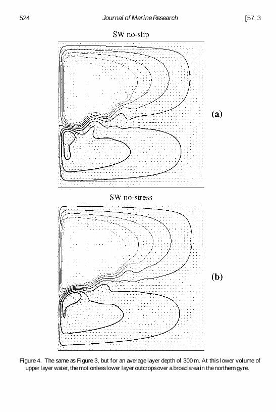
Figure 4. The same as Figure 3, but for an average layer depth of 300 m. At this lower volume ofupper layer water, the motionless lower layer outcrops over a broad area in the northern gyre.


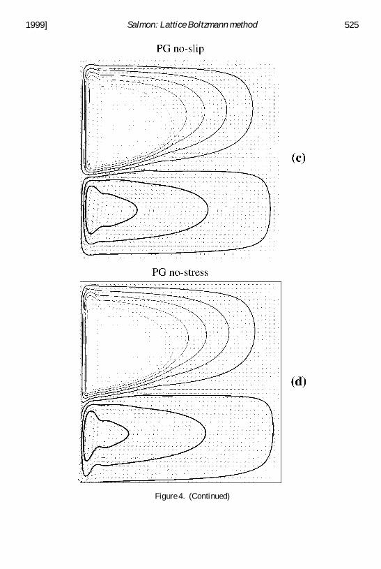
Figure 4. (Continued)


Like the full shallow water equations (4.2–3), the system (4.3, 4.6) contains inertia-gravity waves; the linearized approximations to both systems are identical. Thus, bothsystems contain the same number of fast and slow modes, and both systems demand aboutthe same amount of computation. (Because of the need for predictor/corrector, thestreaming step uses the most processor time, so the time saved by not calculating the O(u2)terms in (3.13–15) is relatively insigni� cant.) Beyond the comparison between SW and PGsolutions, what then is gained by throwing out the momentum advection?

5. The 4-velocity model

I believe there are two advantages to the omission of momentum advection. Oneadvantage has a physical basis; the other is computational.Both advantages are likely to bemuch more signi� cant in three dimensions than in two dimensions, but it is worthwhile toconsider them here. We consider the physical advantage of PG in the following section anddevote this section to the computational advantage.

The computational advantage of (4.6) arises from the fact that the corresponding LBmodel requires only 4 nonzero velocities at each lattice point. Refer to Figure 5a. Includingthe rest particle, this 4-velocity model contains only 5 (instead of 9) modes, and only 2 ofthe 5 modes are fast modes in the sense of Section 2.

The 4-velocity model of Figure 5 cannot be used for the physics (3.13–15) containingmomentum advection, because its lower degree of isotropy leads to a completely incorrectrepresentation of the momentum � ux tensor.2 For example, it is intuitivelyobvious that the4-velocity model cannot represent the northward advection of eastward momentumbecause the 4-velocity model lacks diagonal links; the northward moving particles have noeastward momentum, and vice versa. In the full shallow water equations, this de� ciency isassociated with the existence of spurious line invariants, that is, with the conservation, in

2. The need for a lattice with sufficient symmetry to represent the desired physics was � rst recognized byFrisch et al. (1986); their classic paper inspired much of the subsequent interest in lattice gases and relatedmethods like LB.

Table 1. Summary of numerical experiments.

Fig. Dynamics Average h B. cond. Yearsh min(max)

Maximum* hu *

s (n) gyretransports

3a SW 500 m no-slip 40 100m (687 m) 0.20 Sv km2 1 25.3 Sv (22.4 Sv)3b SW 500 no-stress 60 87 (697) 0.30 26.4 (23.8)3c PG 500 no-slip 30 44 (695) 0.20 26.4 (24.0)3d PG 500 no-stress 60 5 (710) 0.33 28.7 (24.6)4a SW 300 m no-slip 55 5 (582) 0.17 25.6 (11.3)4b SW 300 no-stress 85 5 (597) 0.22 26.9 (11.9)4c PG 300 no-slip 40 5 (550) 0.17 21.9 (11.3)4d PG 300 no-stress 40 5 (560) 0.26 22.7 (11.9)6a PG-4 500 m no-normal 40 173 (674) 0.41 22.7 (21.2)6b PG-4 300 m � ow 60 5 (531) 0.31 19.3 (11.3)


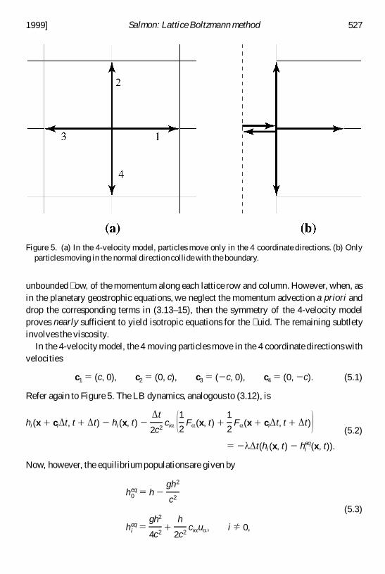
unbounded � ow, of the momentum along each lattice row and column. However, when, asin the planetary geostrophic equations, we neglect the momentum advection a priori anddrop the corresponding terms in (3.13–15), then the symmetry of the 4-velocity modelproves nearly sufficient to yield isotropic equations for the � uid. The remaining subtletyinvolves the viscosity.

In the 4-velocity model, the 4 moving particles move in the 4 coordinate directions withvelocities

c1 5 (c, 0), c2 5 (0, c), c3 5 ( 2 c, 0), c4 5 (0, 2 c). (5.1)

Refer again to Figure 5. The LB dynamics, analogous to (3.12), is

hi(x 1 ci D t, t 1 D t) 2 hi(x, t) 2D t

2c2cia 1 12 Fa (x, t) 1

1

2F a (x 1 ciD t, t 1 D t)2

5 2 l D t(hi(x, t) 2 hieq(x, t)).

(5.2)

Now, however, the equilibrium populations are given by

h0eq 5 h 2

gh2

c2

h ieq 5

gh2

4c21

h

2c2cia u a , i Þ 0,

(5.3)

Figure 5. (a) In the 4-velocity model, particles move only in the 4 coordinate directions. (b) Onlyparticles moving in the normal direction collide with the boundary.


which contain no O(u2) terms. The equilibrium populations (5.3) satisfy (3.16), (3.17), and

oi

cia ci b h ieq 5

1

2gh2d a b , (5.4)

the analog of (3.18).Once again, we may use the Chapman-Enskog expansion to derive equations for the

slow modes. However, because the 4-velocity model contains only 2 fast modes, it is moreinteresting to follow the � rst of the two methods illustrated in Section 2—the expansion inD t alone. To the � rst order in D t, (5.2) implies

1 t1 ci a

x a2 hi 5

1

2c2ci a Fa 2 l (hi 2 h i

eq). (5.5)

As usual, we obtain the slow mode equations from the weighted sums of (5.5). Summing(5.5) from i 5 0 to 4 yields the continuityequation (4.3); summing ci a times (5.5) yields themomentum equation

t(hu a ) 1

R a b

x b5 F a , (5.6)

where

R a b ; oi

ci a cib hi (5.7)

and F a is given by (4.1). At equilibrium, (5.7) takes the value (5.4); as in Section 3, thedifference between (5.7) and (5.4) is the viscous tensor. In the 4-velocity model,

R11 5 c2(h1 1 h3), R22 5 c2(h2 1 h4), R12 5 R21 5 0. (5.8)

Thus it is convenient to take R11 and R22 as the remaining two (fast) modes of the LBsystem. Directly from (5.5), we obtain the fast mode equations

R11

t1 c2

(hu)

x5 2 l (R11 2 R11

eq)

R22

t1 c2

(hv)

y5 2 l (R22 2 R22

eq).

(5.9)

Eqs. (5.6) and (5.9) are analogous to (2.14) and (2.10), respectively.Eq. (4.3, 5.6, 5.9) forma complete set of equations for all 5 modes. Eliminating R11 and R22 between (5.9) and(5.6), we obtain the analogs of (2.17),

l [(hu)t 2 fhv 1 ghhx] 1 [(hu)tt 2 f (hv)t 2 c2(hu)xx] 5 0

l [(hv)t 1 fhu 1 ghhy] 1 [(hv)tt 1 f (hu)t 2 c2(hv)yy] 5 0(5.10)


in which, for simplicity, we have temporarily dropped the wind forcing terms. As inSection 2, the leading order LB dynamics corresponds to l times the equations of interestplus ‘‘textbook’’ wave equations, now modi� ed by rotation.

For small time step and lattice spacing, the 4-velocity LB dynamics (5.2–3) is equivalentto (4.3) and (5.10). For large enough l and c, solutions of (5.10) approximately satisfy

(hu)t 2 fhv 5 2 ghhx 1 n (hu)xx

(hv)t 1 fhu 5 2 ghhy 1 n (hv)yy

(5.11)

where n 5 c2/ l . Eqs. (5.11) are analogous to (2.20). The Chapman-Enskog expansion alsoyields (5.11), but with the more accurate value

n 5 1 1l 21

l max2 c2, (5.12)

where l max 5 2/ D t as before. Eq. (5.12) is analogous to (4.4). The momentum equations(5.11) differ from (4.6) only in the form of the viscosity, which is anisotropic in (5.11). Thisanisotropy results from the relatively low degree of symmetry of the 4-velocity lattice.

As in the case of (4.6), LB solutions of (5.11) always approach a steady state. In steadystate, = · (hu) 5 0, and the transport is described by a streamfunction: hu 5 ( 2 c y, c x). Inthe case of (4.6), the streamfunction satis� es

b c x 5 curl 1 h

h 1 d Et 2 1 n = 4c (5.13)

with boundary conditions of no-normal-� ow, and no-slip or no-stress. If h is everywheremuch greater than d E, then (5.13) reduces to Munk’s classic equation, and c is determinedindependently of h; in fact, the 8-velocity PG solution of Figure 3c closely resemblesMunk’s solution.

In the case of (5.11), the streamfunction satis� es

b c x 5 curl 1 h

h 1 d Et 2 1 2 n c xxyy. (5.14)

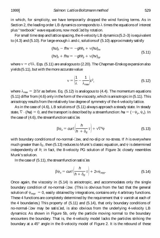
Once again, the viscosity in (5.14) is anisotropic, and accommodates only the singleboundary condition of no-normal-� ow. (This is obvious from the fact that the generalsolution of c xxyy 5 0, easily obtained by integrations, contains only 4 arbitrary functions.These 4 functions are completely determined by the requirement that c vanish at each ofthe 4 boundaries.) This property of (5.11) and (5.14), that only boundary conditions ofno-normal-� ow may be satis� ed, is also obvious from the underlying 4-velocity LBdynamics: As shown in Figure 5b, only the particle moving normal to the boundaryencounters the boundary. That is, the 4-velocity model lacks the particles striking theboundary at a 45° angle in the 8-velocity model of Figure 2. It is the rebound of these


particles that determines the second boundary condition, no slip or no stress, in the8-velocity model.

In the case of (5.13), the western boundary layer equation contains only x-derivatives; itsthickness is d M 5 ( n / b )1/3. However, in the case of (5.14), the western boundary layerequation is a partial differential equation,

b c x 5 2n c xxyy. (5.15)

From (5.15) we see that the western boundary layer thickness is

d s 52 n

b l2, (5.16)

where l is the scale for long-shore variation in c , determined by the interior solution.Thus,in the case of the 4-velocity model, the western boundary layer is proportional to theviscosity coefficient, as in Stommel’s classic ‘‘bottom friction’’ model.

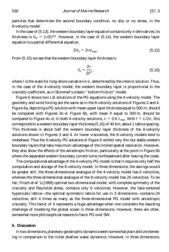
Figure 6 shows two LB solutions of the PG equations using the 4-velocity model. Thegeometry and wind forcing are the same as in the 8-velocity solutions of Figures 3 and 4.Figure 6a, depicting a PG solution with mean upper layer thickness equal to 500 m, shouldbe compared with Figures 3c–d. Figure 6b, with mean h equal to 300 m, should becompared to Figure 4c–d. In both 4-velocity solutions, l 5 0.6 l max. With l 5 L/2p , thiscorresponds to a western boundary layer thickness (5.16) of 40 km, about 1 lattice spacing.This thickness is about half the western boundary layer thickness of the 8-velocitysolutions shown in Figures 3 and 4. At lower viscosities, the 8-velocity models tend tomisbehave. Thus the 4-velocity PG solutions of Figure 6 exhibit very thin but stable westernboundary layers that take maximum advantage of the limited spatial resolution. However,they also show the effects of the anisotropic friction, particularly at the point in Figure 6bwhere the separated western boundary current turns northeastward after leaving the coast.

The computational advantage of the 4-velocity PG model is that it requires only half thecomputation and storage of the 8-velocity model. In three dimensions, the savings wouldbe greater still; the three-dimensional analogue of the 4-velocity model has 6 velocities,whereas the three-dimensional analogue of the 8-velocity model has 26 velocities. To befair, Frisch et al.’s (1986) optimal two-dimensional model, with complete symmetry of theviscosity and Reynolds stress, contains only 6 velocities. However, the face-centeredhypercubic lattice—the optimal symmetric lattice for use in 3 dimensions—contains 24velocities, still 4 times as many as the three-dimensional PG model with anisotropicviscosity. This factor of 4 represents a huge advantage when one considers the dauntingchallenge of modeling the global ocean in three dimensions. However, there are other,somewhat more philosophical reasons to favor PG over SW.

6. Discussion

In two dimensions,planetary geostrophic dynamics seem somewhat plain and uninterest-ing in comparison to the richer shallow water dynamics. However, in three dimensions,


Figure 6. Solutions of the reduced gravity model based upon planetary geostrophicdynamics and the4-velocitymodel of Section 5. The forcing and geometry are the same as in the 8-velocitysolutionsof Figures 3 and 4, but the viscosity now re� ects the anisotropyof the underlying lattice. (a) Meanupper layer depth h of 500 m. (b) Mean h of 300 m.


with bathymetry of realistic complexity, solving and understanding planetary geostrophicdynamics will prove to be a considerable challenge. In three dimensions, even lineardynamics offer a signi� cant computational challenge; see Salmon (1998b).

The primitive equations (PE)—the three-dimensional analogues of the shallow waterequations—may simply be too complex for the present level of dynamical understandingand computational power. In fact, three-dimensional PE admit such a vast range ofphenomena that it is conceivable that PE performance may actually degrade as modelresolution increases, unless the eddy viscosity is unrealistically large, or the viscous cutofffor molecular viscosity is resolved—an utter impossibility.

For example, consider small-scale Kelvin-Helmholtz instability, an apparently ubiqui-tous phenomenon in the atmosphere and ocean. If model resolution reaches the point wheresuch instability can occur but is still too coarse to resolve the turbulent cascade that dampsthe instability, then the instability could become a damaging source of computationalnoise.3

In any case, considering the present state of ignorance about global ocean dynamics, itwould seem safest to begin three-dimensional LB modeling with PG dynamics. Thethree-dimensional analogue of the 4-velocity model in Section 5 offers the advantages ofdynamical and computational simplicity, massively parallel construction, and only slightlymore dependent variables than in traditional primitive equation models.

Signi� cant difficulties remain. The present method of incorporating the Coriolis force,which makes the LB equations implicit and forces us to use the predictor/corrector method,is accurate but inefficient. I have not yet found an acceptable alternative. A much greaterdifficulty is that the complex shapes of the real ocean basins seem to require an irregularlattice. Unfortunately, LB methods do not adapt well to irregular lattices. Even theseemingly unavoidable practice of choosing the vertical lattice spacing to be much smallerthan the horizontal spacing complicates the LB approach. However, with time andpersistence, these difficulties will be overcome. The efficiency and physical simplicity ofLB methods are too great to be ignored.

In more conventional numerical modeling, one begins with a relatively simple set ofpartial differential equations, but the � nal algorithm is a complicated patchwork ofarbitrary steps and compromises that bears only a nebulous relationship to the originaldifferential equations. In the LB method, the algorithm always takes a simple form, anditself acquires the status of an interesting physical system. To investigate its relation todifferential equations, we must pursue a relatively complicated analytical expansion, butthis is a separate activity, necessary only because of our psychological need to associatemodels with differential equations.

Acknowledgments. This work was supported by the National Science Foundation, grant OCE-9521004. It is a pleasure to thank Glenn Ierley and George Veronis for helpful comments, and BreckBetts for his help with the � gures.

3. Similar ideas were expressed to me by M. J. P. Cullen.


APPENDIX

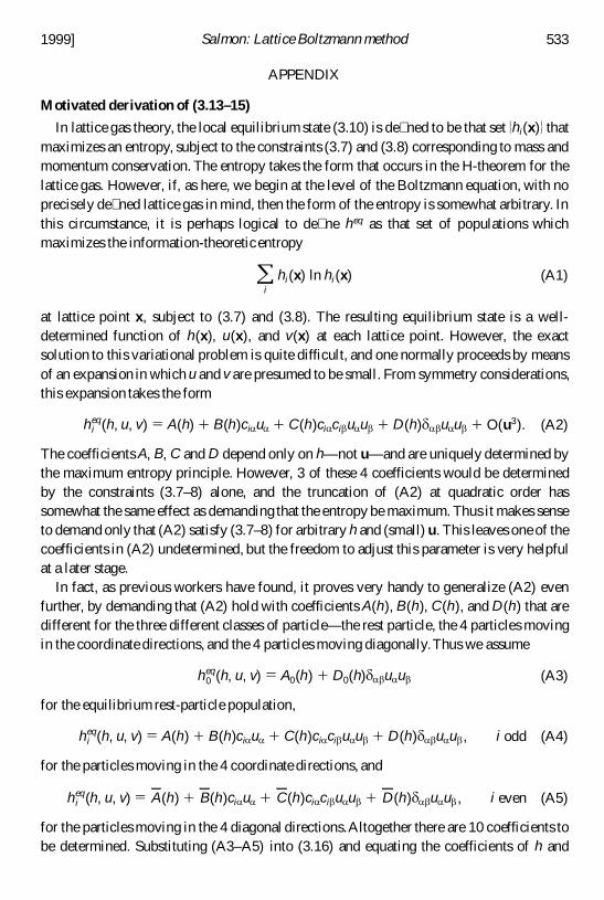
Motivated derivation of (3.13–15)

In lattice gas theory, the local equilibrium state (3.10) is de� ned to be that set 5 hi(x) 6 thatmaximizes an entropy, subject to the constraints (3.7) and (3.8) corresponding to mass andmomentum conservation. The entropy takes the form that occurs in the H-theorem for thelattice gas. However, if, as here, we begin at the level of the Boltzmann equation, with noprecisely de� ned lattice gas in mind, then the form of the entropy is somewhat arbitrary. Inthis circumstance, it is perhaps logical to de� ne heq as that set of populations whichmaximizes the information-theoretic entropy

oi

hi(x) ln hi(x) (A1)

at lattice point x, subject to (3.7) and (3.8). The resulting equilibrium state is a well-determined function of h(x), u(x), and v(x) at each lattice point. However, the exactsolution to this variational problem is quite difficult, and one normally proceeds by meansof an expansion in which u and v are presumed to be small. From symmetry considerations,this expansion takes the form

h ieq(h, u, v) 5 A(h) 1 B(h)cia ua 1 C(h)ci a cib ua u b 1 D(h) d a b u a u b 1 O(u3). (A2)

The coefficients A, B, C and D depend only on h—not u—and are uniquely determined bythe maximum entropy principle. However, 3 of these 4 coefficients would be determinedby the constraints (3.7–8) alone, and the truncation of (A2) at quadratic order hassomewhat the same effect as demanding that the entropy be maximum. Thus it makes senseto demand only that (A2) satisfy (3.7–8) for arbitrary h and (small) u. This leaves one of thecoefficients in (A2) undetermined, but the freedom to adjust this parameter is very helpfulat a later stage.

In fact, as previous workers have found, it proves very handy to generalize (A2) evenfurther, by demanding that (A2) hold with coefficients A(h), B(h), C(h), and D(h) that aredifferent for the three different classes of particle—the rest particle, the 4 particles movingin the coordinate directions, and the 4 particles moving diagonally.Thus we assume

h0eq(h, u, v) 5 A0(h) 1 D0(h) d a b u a u b (A3)

for the equilibrium rest-particle population,

h ieq(h, u, v) 5 A(h) 1 B(h)cia u a 1 C(h)cia cib u a u b 1 D(h) d a b u a u b , i odd (A4)

for the particles moving in the 4 coordinate directions, and

h ieq(h, u, v) 5 A(h) 1 B(h)ci a ua 1 C(h)ci a cib u a u b 1 D(h) d a b u a ub , i even (A5)

for the particles moving in the 4 diagonal directions.Altogether there are 10 coefficients tobe determined. Substituting (A3–A5) into (3.16) and equating the coefficients of h and


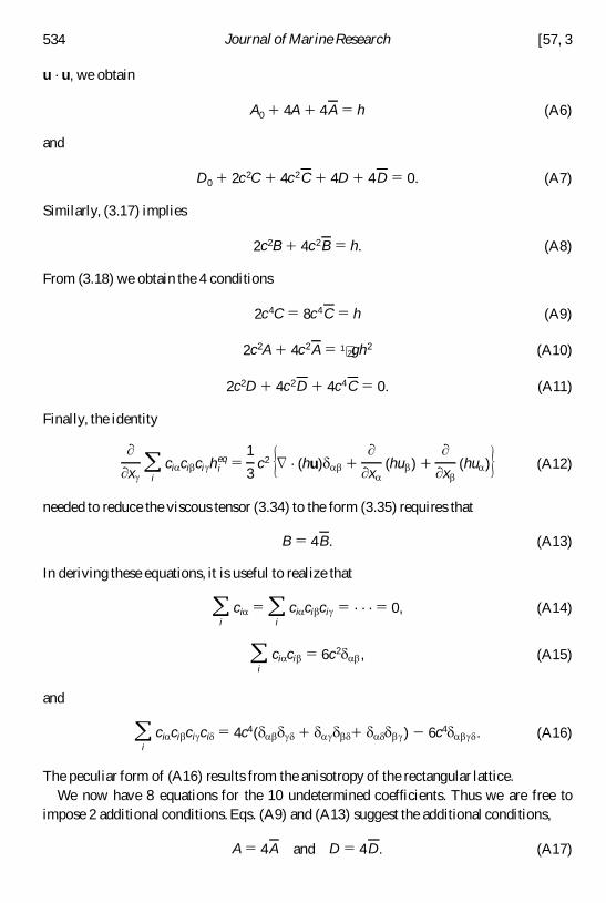
u · u, we obtain

A0 1 4A 1 4A 5 h (A6)

and

D0 1 2c2C 1 4c2C 1 4D 1 4D 5 0. (A7)

Similarly, (3.17) implies

2c2B 1 4c2B 5 h. (A8)

From (3.18) we obtain the 4 conditions

2c4C 5 8c4C 5 h (A9)

2c2A 1 4c2A 5 1�2gh2 (A10)

2c2D 1 4c2D 1 4c4C 5 0. (A11)

Finally, the identity

xgo

ici a cib ci g h i

eq 51

3c2 5 = · (hu) d a b 1

x a(hu b ) 1

xb(hua ) 6 (A12)

needed to reduce the viscous tensor (3.34) to the form (3.35) requires that

B 5 4B. (A13)

In deriving these equations, it is useful to realize that

oi

cia 5 oi

cia ci b cig 5 · · · 5 0, (A14)

oi

ci a ci b 5 6c2 d a b , (A15)

and

oi

cia ci b cig cid 5 4c4( d a b d g d 1 d a g d b d 1 d a d d b g ) 2 6c4 d a b g d . (A16)

The peculiar form of (A16) results from the anisotropy of the rectangular lattice.We now have 8 equations for the 10 undetermined coefficients. Thus we are free to

impose 2 additional conditions. Eqs. (A9) and (A13) suggest the additional conditions,

A 5 4A and D 5 4D. (A17)


These make all the coefficients in (A5) one fourth the size of the corresponding coefficientsin (A4). Then, solving for all the coefficients, we obtain (3.13–15). Note that, forsufficiently small positive h, half of the populations (3.14–15) actually become negative.

REFERENCESAncona, M. G. 1994. Fully-Lagrangian and Lattice-Boltzmann methods for solving systems of

conservationequations. J. Comp. Phys., 115, 107–120.Benzi, R., S. Succi and M. Vergassola. 1992. The lattice Boltzmann-equation—theory and applica-

tions. Phys. Rep., 222, 145–197.Benzi, R., F. Toschi and R. Tripiccione. 1998. On the heat transfer in Rayleigh-Benard systems. J.

Stat. Phys., 93, 901–918.Chen, S. and G. D. Doolen. 1998. Lattice Boltzmann method for � uid � ows. Ann. Rev. Fluid Mech.,

30, 329–364.Frisch, U., B. Hasslacher and Y. Pomeau. 1986. Lattice-gas automata for the Navier-Stokes

equations.Phys. Rev. Lett., 56, 1505–1508.Parsons,A. T. 1969.A two-layer model of Gulf Stream separation. J. Fluid Mech., 39, 511–528.Rothman, D. H. and S. Zaleski. 1997. Lattice-Gas Cellular Automata: Simple Models of Complex

Hydrodynamics,Cambridge, 297 pp.Salmon, R. 1998a. Lectures on Geophysical Fluid Dynamics, Oxford, 378 pp.—— 1998b. Linear ocean circulation theory with realistic bathymetry. J. Mar. Res., 56, 833–884.Veronis, G. 1973. Model of world ocean circulation: I. Wind-driven, two-layer. J. Mar. Res., 31,

228–288.—— 1980. Dynamics of large-scaleocean circulation, in Evolution of Physical Oceanography,B. A.

Warren and C. Wunsch, eds., 140–183.

Received: 6 October, 1998; revised: 9 February, 1999.


Documents

The lattice Boltzmann method as a basis for ocean ...rsalmon/salmon.1999a.pdf · Numerical ocean circulation modelers usually follow one of two strategies. Numerical models based