Ocean Modelling 86 (2015) 15–35

Contents lists available at ScienceDirect

Ocean Modelling

journal homepage: www.elsevier .com/locate /ocemod

Stochastic simulations of ocean waves: An uncertainty quantificationstudy

http://dx.doi.org/10.1016/j.ocemod.2014.12.0011463-5003/� 2014 Elsevier Ltd. All rights reserved.

⇑ Corresponding author. Tel.: +1 650 723 3120.E-mail address: yildirim@stanford.edu (B. Yildirim).

B. Yildirim a,⇑, George Em Karniadakis b

a Department of Geophysics, Stanford University, Stanford, CA 94305, USAb Division of Applied Mathematics, Brown University, Providence, RI 02912, USA

a r t i c l e i n f o a b s t r a c t

Article history:Received 20 June 2014Received in revised form 29 November 2014Accepted 3 December 2014Available online 15 December 2014

Keywords:Ocean wave modelingUncertainty quantificationGeneralized polynomial chaosSparse grid collocationSensitivity analysisKarhunen–Loeve decomposition

The primary objective of this study is to introduce a stochastic framework based on generalized polynomialchaos (gPC) for uncertainty quantification in numerical ocean wave simulations. The techniques wepresent can be easily extended to other numerical ocean simulation applications. We perform stochasticsimulations using a relatively new numerical method to simulate the HISWA (Hindcasting Shallow WaterWaves) laboratory experiment for directional near-shore wave propagation and induced currents in ashallow-water wave basin. We solve the phased-averaged equation with hybrid discretization basedon discontinuous Galerkin projections, spectral elements, and Fourier expansions. We first validate thedeterministic solver by comparing our simulation results against the HISWA experimental data as wellas against the numerical model SWAN (Simulating Waves Nearshore). We then perform sensitivity anal-ysis to assess the effects of the parametrized source terms, current field, and boundary conditions. Weemploy an efficient sparse-grid stochastic collocation method that can treat many uncertain parameterssimultaneously. We find that the depth-induced wave-breaking coefficient is the most important param-eter compared to other tunable parameters in the source terms. The current field is modeled as randomprocess with large variation but it does not seem to have a significant effect. Uncertainty in the sourceterms does not influence significantly the region before the submerged breaker whereas uncertainty inthe incoming boundary conditions does. Considering simultaneously the uncertainties from the sourceterms and boundary conditions, we obtain numerical error bars that contain almost all experimentaldata, hence identifying the proper range of parameters in the action balance equation.

� 2014 Elsevier Ltd. All rights reserved.

1. Introduction

We first present an overview of the action balance equationalong with the numerical model, a description of the HISWAexperiment, and a review of the stochastic modeling approachwe employ. We then present the objectives of this work and theorganization of the rest of the paper.

1.1. Phase-averaged equation and source terms

We model ocean waves through the spectral ocean waveequation (Holthuijsen, 2007; Young, 1999) also referred to it asphased-averaged model. We solve for the energy density (or actiondensity) to obtain important statistical wave parameters, such asthe significant wave height, mean wave period, etc. The phase-averaged model is well suited for slowly varying wave fields, such

as ocean waves in deep water, and it is more appropriate for largespatial domains (Battjes, 1994). In contrast, the model simulatingthe surface elevation in space and time is called phase-resolving,and is more efficient for waves in a small region of the sea suchas a harbor (Battjes, 1994). The spectral ocean representation isessentially a superimposition of many different linear harmonicwaves to represent complex ocean surface waves.

Today, most operational ocean codes employ the phase-averaged model. Some of the most well-known codes are SWAN(Simulating Waves Near-Shore) available from http://www.swan.tudelft.nl/, ECWAM (European Center Wave Model)available from http://www.ecmwf.int/, and NOAA’s WAVEWATCHavailable from http://polar.ncep.noaa.gov/waves/. These estab-lished operational wave codes employ up to third-order of finitedifference discretization in Tolman (1995) for spatial derivatives.To be able to construct arbitrary order of discretization with thisnew scheme is its biggest advantage over the traditional discretiza-tion methods. Although finite difference on structured mesh is anestablished and efficient method and relatively easy to implement,

16 B. Yildirim, G.E. Karniadakis / Ocean Modelling 86 (2015) 15–35

it is not well suited for complex geometries, e.g. in coastal applica-tions. Recent effort to use finite difference on unstructured meshfor spectral wave model can be found in the work of Zijlema(2010). On the other hand, the finite element (FE) and finite vol-ume (FV) methods that work on a general grid offer an accurateand efficient algorithm. Recent works have incorporated thesemethods into the wave models to handle complex coastal bound-aries (Hsu et al., 2005; Qi et al., 2009).

1.2. High-order numerical model

Recently we introduced a new numerical method for the spec-tral ocean wave equations (Yildirim and Karniadakis, 2012), whichis distinctively different from previous approaches (Booij et al.,1999; Hsu et al., 2005; Qi et al., 2009; Zijlema, 2010) and employshigh-order discretization. Specifically, we compute the spectralspace derivatives by Fourier-collocation while we discretize thephysical space using a discontinuous Galerkin (DG) method(Yildirim and Karniadakis, 2012; Karniadakis and Sherwin, 1999;Hesthaven and Warburton, 2007; Cockburn et al., 2000). The DGdiscretization in geophysical space is performed on an unstruc-tured grid to handle the complex boundaries. The overall schemehas exponential convergence rather than algebraic convergencetypical of low-order schemes. We have verified the exponentialconvergence in both the geophysical and spectral spaces in previ-ous work (Yildirim and Karniadakis, 2012). The low-order methodsassociated with strong numerical dissipation and phase errorssmear out the amplitude of solution and shift the position of it.In long time integrations, the accumulated numerical dissipationand phase errors become so large that accurate simulation is notpossible. Numerical diffusion test case for first order scheme pre-sented in Booij et al. (1999) shows that first-order scheme is notsuitable for the long distance wave propagation. High-order dis-cretization is particularly effective for long-time integration, whichis typically required to eliminate the associated dissipation andphase errors in the deep ocean wave simulations.

1.3. HISWA tank experiment

The HISWA experiment (Dingemans, 1987; Dingemans et al.,1986) is a laboratory experiment conducted for random, short-crested waves to validate numerical spectral ocean models(Holthuijsen et al., 1989). This is benchmark experiment that pro-vides measurements for comparisons with simulations and it isone of the most comprehensive works for wave propagation in a

10

5

0

-5

-10

y (

m)

0 5 10 20 25 30x (m)

Depth (m)

(a) sensors

-

y (m

)

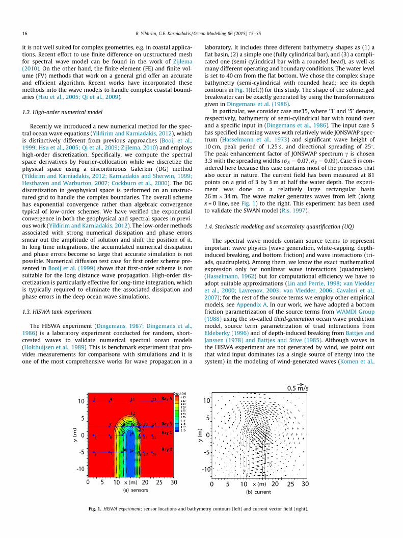
Fig. 1. HISWA experiment: sensor locations and bathym

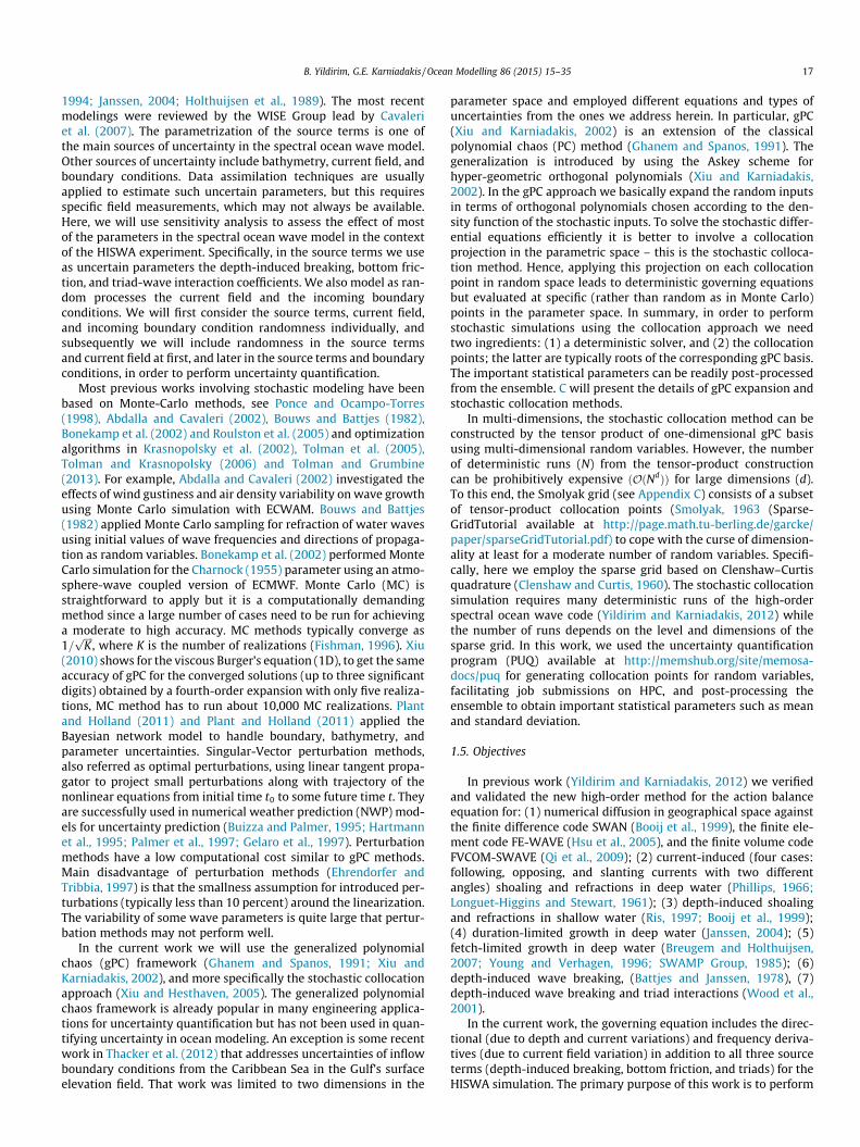
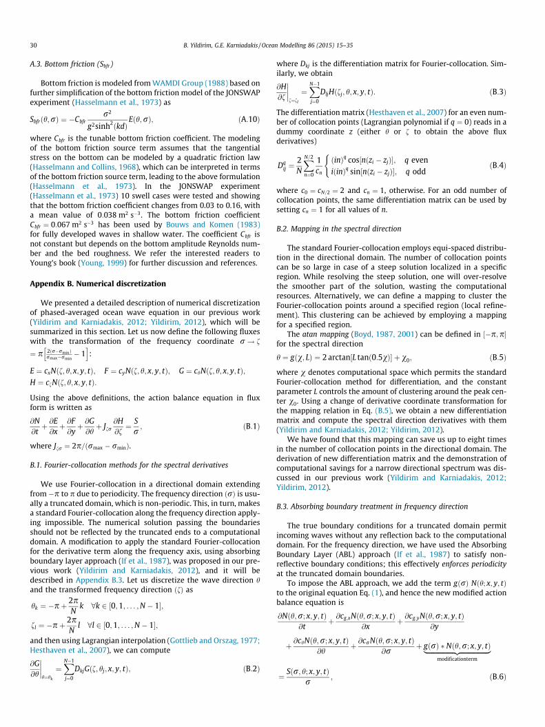
laboratory. It includes three different bathymetry shapes as (1) aflat basin, (2) a simple one (fully cylindrical bar), and (3) a compli-cated one (semi-cylindrical bar with a rounded head), as well asmany different operating and boundary conditions. The water levelis set to 40 cm from the flat bottom. We chose the complex shapebathymetry (semi-cylindrical with rounded head; see its depthcontours in Fig. 1(left)) for this study. The shape of the submergedbreakwater can be exactly generated by using the transformationsgiven in Dingemans et al. (1986).

In particular, we consider case me35, where ‘3’ and ‘5’ denote,respectively, bathymetry of semi-cylindrical bar with round overand a specific input in (Dingemans et al., 1986). The input case 5has specified incoming waves with relatively wide JONSWAP spec-trum (Hasselmann et al., 1973) and significant wave height of10 cm, peak period of 1.25 s, and directional spreading of 25�.The peak enhancement factor of JONSWAP spectrum c is chosen3.3 with the spreading widths ðrA ¼ 0:07;rB ¼ 0:09Þ. Case 5 is con-sidered here because this case contains most of the processes thatalso occur in nature. The current field has been measured at 81points on a grid of 3 by 3 m at half the water depth. The experi-ment was done on a relatively large rectangular basin26 m� 34 m. The wave maker generates waves from left (alongx = 0 line, see Fig. 1) to the right. This experiment has been usedto validate the SWAN model (Ris, 1997).

1.4. Stochastic modeling and uncertainty quantification (UQ)

The spectral wave models contain source terms to representimportant wave physics (wave generation, white-capping, depth-induced breaking, and bottom friction) and wave interactions (tri-ads, quadruplets). Among them, we know the exact mathematicalexpression only for nonlinear wave interactions (quadruplets)(Hasselmann, 1962) but for computational efficiency we have toadopt suitable approximations (Lin and Perrie, 1998; van Vledderet al., 2000; Lavrenov, 2003; van Vledder, 2006; Cavaleri et al.,2007); for the rest of the source terms we employ other empiricalmodels, see Appendix A. In our work, we have adopted a bottomfriction parametrization of the source terms from WAMDI Group(1988) using the so-called third-generation ocean wave predictionmodel, source term parametrization of triad interactions fromEldeberky (1996) and of depth-induced breaking from Battjes andJanssen (1978) and Battjes and Stive (1985). Although waves inthe HISWA experiment are not generated by wind, we point outthat wind input dominates (as a single source of energy into thesystem) in the modeling of wind-generated waves (Komen et al.,

10

5

0

-5

10

0 5 10 20 3025x (m)

0.5 m/s

(b) current

etry contours (left) and current vector field (right).

B. Yildirim, G.E. Karniadakis / Ocean Modelling 86 (2015) 15–35 17

1994; Janssen, 2004; Holthuijsen et al., 1989). The most recentmodelings were reviewed by the WISE Group lead by Cavaleriet al. (2007). The parametrization of the source terms is one ofthe main sources of uncertainty in the spectral ocean wave model.Other sources of uncertainty include bathymetry, current field, andboundary conditions. Data assimilation techniques are usuallyapplied to estimate such uncertain parameters, but this requiresspecific field measurements, which may not always be available.Here, we will use sensitivity analysis to assess the effect of mostof the parameters in the spectral ocean wave model in the contextof the HISWA experiment. Specifically, in the source terms we useas uncertain parameters the depth-induced breaking, bottom fric-tion, and triad-wave interaction coefficients. We also model as ran-dom processes the current field and the incoming boundaryconditions. We will first consider the source terms, current field,and incoming boundary condition randomness individually, andsubsequently we will include randomness in the source termsand current field at first, and later in the source terms and boundaryconditions, in order to perform uncertainty quantification.

Most previous works involving stochastic modeling have beenbased on Monte-Carlo methods, see Ponce and Ocampo-Torres(1998), Abdalla and Cavaleri (2002), Bouws and Battjes (1982),Bonekamp et al. (2002) and Roulston et al. (2005) and optimizationalgorithms in Krasnopolsky et al. (2002), Tolman et al. (2005),Tolman and Krasnopolsky (2006) and Tolman and Grumbine(2013). For example, Abdalla and Cavaleri (2002) investigated theeffects of wind gustiness and air density variability on wave growthusing Monte Carlo simulation with ECWAM. Bouws and Battjes(1982) applied Monte Carlo sampling for refraction of water wavesusing initial values of wave frequencies and directions of propaga-tion as random variables. Bonekamp et al. (2002) performed MonteCarlo simulation for the Charnock (1955) parameter using an atmo-sphere-wave coupled version of ECMWF. Monte Carlo (MC) isstraightforward to apply but it is a computationally demandingmethod since a large number of cases need to be run for achievinga moderate to high accuracy. MC methods typically converge as1=

ffiffiffiffiKp

, where K is the number of realizations (Fishman, 1996). Xiu(2010) shows for the viscous Burger’s equation (1D), to get the sameaccuracy of gPC for the converged solutions (up to three significantdigits) obtained by a fourth-order expansion with only five realiza-tions, MC method has to run about 10,000 MC realizations. Plantand Holland (2011) and Plant and Holland (2011) applied theBayesian network model to handle boundary, bathymetry, andparameter uncertainties. Singular-Vector perturbation methods,also referred as optimal perturbations, using linear tangent propa-gator to project small perturbations along with trajectory of thenonlinear equations from initial time t0 to some future time t. Theyare successfully used in numerical weather prediction (NWP) mod-els for uncertainty prediction (Buizza and Palmer, 1995; Hartmannet al., 1995; Palmer et al., 1997; Gelaro et al., 1997). Perturbationmethods have a low computational cost similar to gPC methods.Main disadvantage of perturbation methods (Ehrendorfer andTribbia, 1997) is that the smallness assumption for introduced per-turbations (typically less than 10 percent) around the linearization.The variability of some wave parameters is quite large that pertur-bation methods may not perform well.

In the current work we will use the generalized polynomialchaos (gPC) framework (Ghanem and Spanos, 1991; Xiu andKarniadakis, 2002), and more specifically the stochastic collocationapproach (Xiu and Hesthaven, 2005). The generalized polynomialchaos framework is already popular in many engineering applica-tions for uncertainty quantification but has not been used in quan-tifying uncertainty in ocean modeling. An exception is some recentwork in Thacker et al. (2012) that addresses uncertainties of inflowboundary conditions from the Caribbean Sea in the Gulf’s surfaceelevation field. That work was limited to two dimensions in the

parameter space and employed different equations and types ofuncertainties from the ones we address herein. In particular, gPC(Xiu and Karniadakis, 2002) is an extension of the classicalpolynomial chaos (PC) method (Ghanem and Spanos, 1991). Thegeneralization is introduced by using the Askey scheme forhyper-geometric orthogonal polynomials (Xiu and Karniadakis,2002). In the gPC approach we basically expand the random inputsin terms of orthogonal polynomials chosen according to the den-sity function of the stochastic inputs. To solve the stochastic differ-ential equations efficiently it is better to involve a collocationprojection in the parametric space – this is the stochastic colloca-tion method. Hence, applying this projection on each collocationpoint in random space leads to deterministic governing equationsbut evaluated at specific (rather than random as in Monte Carlo)points in the parameter space. In summary, in order to performstochastic simulations using the collocation approach we needtwo ingredients: (1) a deterministic solver, and (2) the collocationpoints; the latter are typically roots of the corresponding gPC basis.The important statistical parameters can be readily post-processedfrom the ensemble. C will present the details of gPC expansion andstochastic collocation methods.

In multi-dimensions, the stochastic collocation method can beconstructed by the tensor product of one-dimensional gPC basisusing multi-dimensional random variables. However, the numberof deterministic runs (N) from the tensor-product constructioncan be prohibitively expensive ðOðNdÞÞ for large dimensions (d).To this end, the Smolyak grid (see Appendix C) consists of a subsetof tensor-product collocation points (Smolyak, 1963 (Sparse-GridTutorial available at http://page.math.tu-berling.de/garcke/paper/sparseGridTutorial.pdf) to cope with the curse of dimension-ality at least for a moderate number of random variables. Specifi-cally, here we employ the sparse grid based on Clenshaw–Curtisquadrature (Clenshaw and Curtis, 1960). The stochastic collocationsimulation requires many deterministic runs of the high-orderspectral ocean wave code (Yildirim and Karniadakis, 2012) whilethe number of runs depends on the level and dimensions of thesparse grid. In this work, we used the uncertainty quantificationprogram (PUQ) available at http://memshub.org/site/memosa-docs/puq for generating collocation points for random variables,facilitating job submissions on HPC, and post-processing theensemble to obtain important statistical parameters such as meanand standard deviation.

1.5. Objectives

In previous work (Yildirim and Karniadakis, 2012) we verifiedand validated the new high-order method for the action balanceequation for: (1) numerical diffusion in geographical space againstthe finite difference code SWAN (Booij et al., 1999), the finite ele-ment code FE-WAVE (Hsu et al., 2005), and the finite volume codeFVCOM-SWAVE (Qi et al., 2009); (2) current-induced (four cases:following, opposing, and slanting currents with two differentangles) shoaling and refractions in deep water (Phillips, 1966;Longuet-Higgins and Stewart, 1961); (3) depth-induced shoalingand refractions in shallow water (Ris, 1997; Booij et al., 1999);(4) duration-limited growth in deep water (Janssen, 2004); (5)fetch-limited growth in deep water (Breugem and Holthuijsen,2007; Young and Verhagen, 1996; SWAMP Group, 1985); (6)depth-induced wave breaking, (Battjes and Janssen, 1978), (7)depth-induced wave breaking and triad interactions (Wood et al.,2001).

In the current work, the governing equation includes the direc-tional (due to depth and current variations) and frequency deriva-tives (due to current field variation) in addition to all three sourceterms (depth-induced breaking, bottom friction, and triads) for theHISWA simulation. The primary purpose of this work is to perform

18 B. Yildirim, G.E. Karniadakis / Ocean Modelling 86 (2015) 15–35

a systematic stochastic analysis to assess the adequacy of theparametrization of the source terms, the effect of the current field,and the inlet boundary conditions in the context of the HISWAexperiment. This analysis may identify a proper parametric rangeto be used in other cases as well.

The paper is organized as follows. First, we briefly present theaction balance equation (phased-averaged model) in Section 2and also briefly describe the new high-order scheme in Section 3.Following this section, we present numerical simulation resultsfor various resolutions on a fixed mesh to show the convergenceof the scheme. Next in Section 5, we apply stochastic collocationto the HISWA simulation to quantify the uncertainty in suchimportant wave parameters as the significant wave height ðHsÞ,mean wave period ðTm01Þ, mean wave direction ð�hÞ, and energyspectra ðEðf ÞÞ. Specifically, we first treat the source parameters(depth-induced breaking, bottom friction, and triads) as randominputs. Subsequently, we add space-dependent random perturba-tions to the current field and study the combined effects of the ran-dom current processes with the random source terms. In the lastpart of Section 5, we introduce space-dependent random perturba-tions to the incoming boundary condition and we examine thecombined effect of uncertain boundary conditions with uncertainsource terms. Finally, we present a brief summary in Section 6.In Appendix A we include some details on the parametrization ofthe source terms, the details of the numerical discretization thatthe deterministic code implements is presented in Appendix B,and Appendix C describes the stochastic simulation tools used inthis study.

2. Governing equation

The action balance equation (Booij et al., 1999) for ocean wavesin the Eulerian framework can be written as

@Nðh;r; x; y; tÞ@t

þ @cxNðh;r; x; y; tÞ@x

þ @cyNðh;r; x; y; tÞ@y

þ @chNðh;r; x; y; tÞ@h

þ @crNðh;r; x; y; tÞ@r

¼ Sðh;r; x; y; tÞr

; ð1Þ

where Nðh;r; x; y; tÞ is the action density defined as the ratio ofenergy Eðh;r; x; y; tÞ to relative frequency r (N ¼ E=r), cx and cy

are the propagation velocities of wave energy in physical ðx� yÞspace, and ch and cr are the propagation velocities in spectralh 2 ½�p;p�; r 2 ½0;1�ð Þ space. The explicit expressions of propaga-

tion velocities ðcx; cy; ch; crÞ can be found in Whitham (1974),Holthuijsen (2007) and Yildirim and Karniadakis (2012)). Thesource term Sðh;r; x; y; tÞ accounts for wave generation, dissipation,and wave interaction mechanisms (see Appendix A). The bottomfriction process ðSb;frÞ with bottom friction coefficient Cbfr ¼ 0:067,the depth-induced breaking process Sbr with c ¼ 0:73, the scalingcoefficient (after Battjes and Janssen, 1978) aBJ ¼ 1:5, and the triadinteractions (Snl3) with the scale factor aEB ¼ 0:5 are all representedin our model. We also refer the interested readers to WAMDI Group(1988), Komen et al. (1984), Young and Verhagen (1996),Holthuijsen (2007) and Yildirim and Karniadakis (2012) for an in-depth discussion of modeling the source terms.

3. Numerical discretization

We present a concise description of the numerical discretiza-tion of phased-averaged ocean wave equation in Appendix B,which we summarize in this section. We use the discontinuousGalerkin (DG) (Hesthaven and Warburton, 2007; Hesthaven et al.,2007; Karniadakis and Sherwin, 1999) method for the geographicalspace. The spatial discretization is defined on an arbitrary triangledomain to support the unstructured grids, which are most suitable

grids for the wave problems on the complex bathymetry andcoastal boundaries. The details can be followed on Appendix B.4.

The directional domain extends from �p to p. We use Fourier-collocation to discretize the directional derivative in Eq. (1). Thesolutions in many applications may have a very narrow directionalspreading; an example is cosmðhÞ directional spreading. We see thatmost of the energy contained in only a very narrow region forhigher values of m. The Fourier-collocation employs equi-spaceddistribution in the directional domain. We have to employ veryhigh resolution to capture the very narrow region and, dependingon the solution steepness, the number of collocation points canbe so large that we cannot afford to run such simulations. Alterna-tively, we define a mapping to cluster the Fourier-collocation pointsaround a specified region (local refinement). We have found thatthis mapping can save us up to eight times in the number of collo-cation points in the directional domain. In case that they are manywave fields in the domain or directional peaks keep moving, thenthe discretization needs a fully adapted directional discretization.The current code is only supporting the static grid that can clusterthe grid points around a single specific point. Dynamic grid andmulti-points support will be implemented in the future.

The frequency domain ranges from 0 to1. We usually truncatethe semi-infinite domain into a finite domain as ½f min; f max�. Thenumerical boundary condition in this domain is non-reflecting.The straightforward Fourier-collocation method cannot be appliedfor non-periodic boundary conditions. However, we can still use aFourier-collocation with an Absorbing Boundary Layer (ABL) for thewave problem of which the energy spectra asymptotically goesto zero toward the tails. Fourier-collocation has been shown tohave advantages over the more traditional Chebyshev method(Boyd, 1988) in the truncated domain. We have used the AbsorbingBoundary Layer (ABL) approach (If et al., 1987) to enforce periodic-ity at the frequency domain ends. To this end, we added a modifiedterm to the main Eq. (1) to solve the problem in an extendeddomain ½f min � ML; f max þ MR� that we obtained by adding theabsorbing layers ML and MR, respectively, on the left (f min) and theright (f max). The modified term takes zero values inside the domainand hence we solve the Eq. (1) backwards. The Absorbing BoundaryLayer function defined in Yildirim and Karniadakis (2012) controlsthe modified term in the absorbing boundary layers and introducesheavy dissipation to smear out the solution. The current code isable to generate logarithmic distribution for the frequency direc-tion when the domain is free of a current field. To define logarith-mic distribution in frequency direction for a problem that has acurrent field with non-zero gradient, we should propose a similarmapping as it is done for the directional grid. Similar to a tan map-ping B.5 used for the directional grid, a log mapping (Boyd, 2001)can create a logarithmic distribution around the specific frequencyin the frequency grid. Since the current code can not generate alogarithmic distribution in the frequency direction for the certaincases, the application of the code is limited for general applica-tions. The disadvantage of using uniform grid that deploys the finerfrequency grid to resolve the high-gradients (in frequency direc-tion) is that it will over-resolve the smooth regions, wasting com-puter resources and increasing computation time. To be moreefficient, this new scheme should define a mapping in frequencygrid that generates a logarithmic distribution of points.

We compute the spectral derivatives for each grid point ðhi;riÞin the spectral space. Each grid point now has an equation in geo-graphical space. We then applied discontinuous Galerkin (DG) dis-cretization (Hesthaven and Warburton, 2007; Hesthaven et al.,2007; Karniadakis and Sherwin, 1999) to this equation. We referthe interested readers to Yildirim and Karniadakis (2012) fordetails of spatial discretization of the action balance equation.

With regards to temporal discretization, we employed second-and third-order (Gottlieb and Shu, 1998), as well as the

B. Yildirim, G.E. Karniadakis / Ocean Modelling 86 (2015) 15–35 19

fourth-order explicit (5-stages) (Spiteri and Steven, 2001) StrongStability Preserving Runge–Kutta (SSP-RK) schemes.

4. Validation studies

4.1. Numerical simulation ðS ¼ Sb;fr þ Sbr þ Snl3Þ

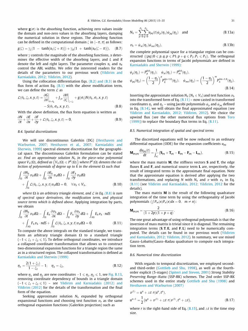
The computational domain in geophysical space (see Fig. 2(a))½ð0;30Þm� ð�45;45Þm� is discretized into 48 triangular elementsin conjunction with a spectral collocation grid whose frequencyaxis ranges from 0.4 Hz to 3.0 Hz with resolution 0.04 Hz (equi-spaced grid along the frequency direction), and the directionaldomain lying in ½�60�;60�� with resolution about 4� around thecenter and about 20� around the tails. The directional collocationpoints are generated by local refinement using the arctan mappingas given in Yildirim and Karniadakis (2012); which clusters the col-location points around the center. The directional domain size½�60�;60�� is sufficient to resolve most of the energy for theme35 case that has directional spreading width given as 25�. Weused a left absorbing boundary layer width as 0.2 Hz and a rightone as 1.0 Hz, which effectively extended the frequency domainfrom ½0:4;3:0� Hz to ½0:2;4:0� Hz.

We applied the incoming energy spectrum on the left boundaryusing the JONSWAP spectrum (see Eq. (7)) with directional spread-ing model cosmðh� h0Þ (Holthuijsen, 2007), where h0 is the refer-ence incoming wave direction and we set m ¼ 4 based on thegiven directional width of 25�. The JONSWAP spectrum(Holthuijsen, 2007; Hasselmann et al., 1973) of peak frequency f p

used here of 0.8 Hz, scale parameter a ¼ 0:0154, peak-widthparameters ra ¼ 0:07 and rb ¼ 0:09 are chosen to represent thesignificant height of 10 cm for the incoming wave boundary condi-tion. The centered reference direction (h0) in the directional distri-bution is interpolated from measurement locations 1–2–3 (alongthe y-axis, see Fig. 1) and projected on the left boundary. Weassume that in the computational boundary outside the ray Aand ray D lines (see Fig. 1) the reference direction (h0) is zero.The lateral boundaries are naturally reflective, but in our imple-mentation we do not take this into account, which is not significantin this case (me35) since in the experiment wave generators send

x (m)

y (

m)

0 10 20 30-45

-30

-15

0

15

30

45

Fig. 2. Computational mesh (48 triangular elements) used for the HISWA simulation. Thedashed region, and the collocation points on this mesh are represented by blue circlesreferred to the web version of this article.)

waves perpendicular (not obliquely) to the left boundary; hence,we specified zero energy along these boundaries. This is inherentlya dissipative process and pollutes the numerical solution inside thedomain. We extended the lateral boundaries ymin to�45 and ymax to45 for minimizing the numerical boundary pollution in the regionof interest (see dashed region in Fig. 2(a)). The experiment wasdesigned to minimize any reflection on the right end and hencewe set non-reflecting boundary conditions at this end. We setthe initial condition to zero energy in the domain for all runs.

The interpolated current field from the experiment wasprovided by N. Booij from Digital Hydraulics Holland (private com-munication). This current field is interpolated to the collocationpoints (see Fig. 2(a) right)) in the simulation. The current field ofthe computational grid outside the experimental area is assumedto be zero; the current vector field is shown in Fig. 1 (right).

Bottom friction and depth-induced wave breaking are theimportant dissipation processes with nonlinear wave-wave inter-actions (only triads). The source parameters are chosen based onthe suggestion of Ris (1997) whose results we used here for theSWAN comparison. Our numerical simulation results verified thatthe important wave parameters are insensitive to quadruplet inter-actions (Snl4), which is also observed in the work of Ris (1997). Qua-druplet interactions are turned off for the HISWA simulation in theentire paper.

The computation is carried out by marching in time (our imple-mentation currently supports only unsteady computation) to reacha steady state solution. To this end, we march the unsteadysolution with the time step 0.025 s up to the final time 35 s. TheRunge–Kutta second-order time integration scheme is employedfor all cases in the entire paper. In space, first-, third-, and fifth-order of the Jacobi polynomials are expanded over the triangularelements in the computation of this section.

The measurement locations of 26 stations are given inFig. 1(left). We have measurements for the significant wave heightHs and mean wave period Tm01 for all 26 locations, but for the meanwave direction �h we have only seven locations (1, 2, 3, 17, 24, 25,26). The comparison is made on horizontal line Rays C and B ratherthan all measurement locations (Rays A, B, C, D) to simplify thepresentation. Extensive results on the Rays A–D can be found in

dashed region (on left) is the experimental region. The mesh (right) is a zoom at the. (For interpretation of the references to colour in this figure legend, the reader is

0 0.5 1 1.5 2 2.5 3

f(Hz)

0

2

4

6

8

10

12

E(f

) (c

m2 /H

z)

HISWA experimentRIS97Structured SWAN Code (2014)Unstructured SWAN Code (2014)DG Code (poly. order = 3)

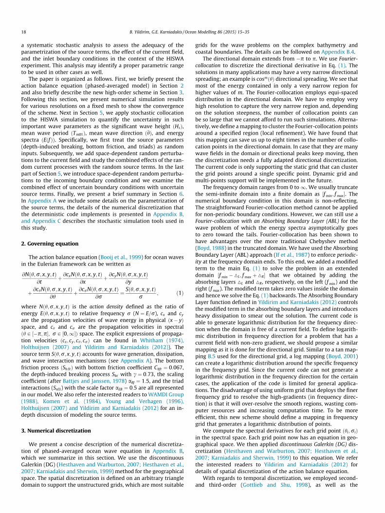
Fig. 4. Energy spectra for the station 24 are presented from HISWA experiment,RIS97 from Ris (1997) (obtained by the earlier version of SWAN code a more than adecade ago), a recent data (2014) from Structured and Unstructured SWAN codes,and DG code (p = 3).

20 B. Yildirim, G.E. Karniadakis / Ocean Modelling 86 (2015) 15–35

Yildirim (2012). The four rays cover 24 stations and exclude onlytwo stations 12 and 17. The energy spectra are compared for eightlocations (5, 3, 13, 15, 16, 19, 24, 26) in this study.

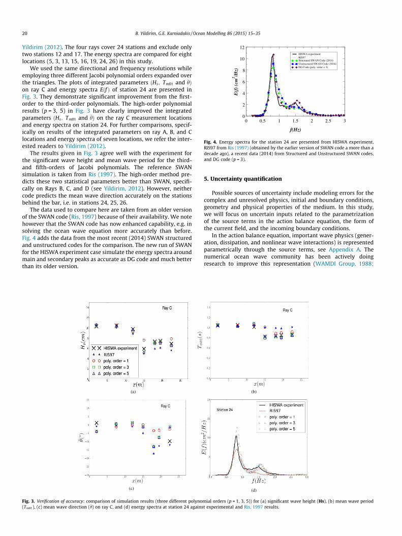
We used the same directional and frequency resolutions whileemploying three different Jacobi polynomial orders expanded overthe triangles. The plots of integrated parameters ðHs; Tm01 and �hÞon ray C and energy spectra Eðf Þ of station 24 are presented inFig. 3. They demonstrate significant improvement from the first-order to the third-order polynomials. The high-order polynomialresults (p = 3, 5) in Fig. 3 have clearly improved the integratedparameters ðHs; Tm01 and �hÞ on the ray C measurement locationsand energy spectra on station 24. For further comparisons, specif-ically on results of the integrated parameters on ray A, B, and Clocations and energy spectra of seven locations, we refer the inter-ested readers to Yildirim (2012).

The results given in Fig. 3 agree well with the experiment forthe significant wave height and mean wave period for the third-and fifth-orders of Jacobi polynomials. The reference SWANsimulation is taken from Ris (1997). The high-order method pre-dicts these two statistical parameters better than SWAN, specifi-cally on Rays B, C, and D (see Yildirim, 2012). However, neithercode predicts the mean wave direction accurately on the stationsbehind the bar, i.e. in stations 24, 25, 26.

The data used to compare here are taken from an older versionof the SWAN code (Ris, 1997) because of their availability. We notehowever that the SWAN code has now enhanced capability, e.g. insolving the ocean wave equation more accurately than before.Fig. 4 adds the data from the most recent (2014) SWAN structuredand unstructured codes for the comparison. The new run of SWANfor the HISWA experiment case simulate the energy spectra aroundmain and secondary peaks as accurate as DG code and much betterthan its older version.

Fig. 3. Verification of accuracy: comparison of simulation results (three different polyno(Tm01), (c) mean wave direction (�h) on ray C, and (d) energy spectra at station 24 agains

5. Uncertainty quantification

Possible sources of uncertainty include modeling errors for thecomplex and unresolved physics, initial and boundary conditions,geometry and physical properties of the medium. In this study,we will focus on uncertain inputs related to the parametrizationof the source terms in the action balance equation, the form ofthe current field, and the incoming boundary conditions.

In the action balance equation, important wave physics (gener-ation, dissipation, and nonlinear wave interactions) is representedparametrically through the source terms, see Appendix A. Thenumerical ocean wave community has been actively doingresearch to improve this representation (WAMDI Group, 1988;

mial orders (p = 1, 3, 5)) for (a) significant wave height (Hs), (b) mean wave periodt experimental and Ris, 1997 results.

B. Yildirim, G.E. Karniadakis / Ocean Modelling 86 (2015) 15–35 21

Cavaleri et al., 2007), and improvements in the source terms arereflected in the so-called first-, second-, and third-generationocean wave models; among them, the third-generation is still themost common model. For the various contributions to the sourceterms, we have an exact mathematical expression for only the qua-druplet wave-wave interactions (Hasselmann, 1962, 1963a,b).Hence, they can be solved exactly as done by Hasselmann andHasselmann (1985), Snyder et al. (1993), Lin and Perrie (1998)and Benoit (2005) but this leads to excessive computational cost.The rest of the important contributions, including dissipation(white-capping, depth-induced breaking, and bottom friction)and triads have no explicit mathematical expressions and theyare modeled empirically in WAMDI Group (1988) through effectiveparameters. Specifically, we will treat the parameters c and aBJ inthe depth-induced wave breaking source term, the bottom frictioncoefficient Cbfr in the bottom friction term, and the triad coefficientaEB in the triad interaction term as random variables.

All runs of our deterministic solver employed third-order Jacobipolynomials on the triangular spectral elements (see mesh inFig. 2(a)). The time integration scheme, boundary condition, andspectral space size and resolution are all kept the same as in theprevious section.

5.1. Sensitivity analysis of source term parameters

The elementary effect method (Morris, 1991) provides a mea-sure of sensitivity from a small number of model evaluations.

Let us consider a function F that has k independent inputparameters such that

F ¼ f ðX1;X2; . . . ;XkÞ;

where X ¼ ðX1;X2; . . . ;XkÞ varies in a k-dimensional cube with plevel, which selects sampling locations on each dimension. The ele-mentary effect is defined as:

dðXiÞ ¼FðX1;X2; . . . ;Xi�1;Xi þ M; . . . ;XkÞ � FðX1;X2; . . . ;XkÞ

M; ð2Þ

where M is a value chosen equal to p=ð2ðp� 1ÞÞ for even p. In thismethod we choose randomly r sample points among p levels(r < p). The number of r samples can be considerably smaller thanp, and hence the method needs k� r output evaluations to computethe sensitivity. The random r sample points can be taken from theSmolyak grid (Smolyak, 1963). The elementary effect method usestwo measures for mean ðlÞ and standard deviation ðrÞ of r elemen-tary effects of each input. The mean ðlÞmeasures the relative influ-ence factor of each input. The mean of r sampling elementary effectsis defined (for input Xi) as

li ¼1r

Xr

j¼1

d XðjÞi

� �: ð3Þ

The standard deviation r assesses nonlinear effects of the inputparameters (Xk) (Saltelli et al., 2008). The software PUQ that weuse has the capability of post-processing output functions to com-pute the mean and standard deviations of r sampled elementaryeffects for the input parameters.

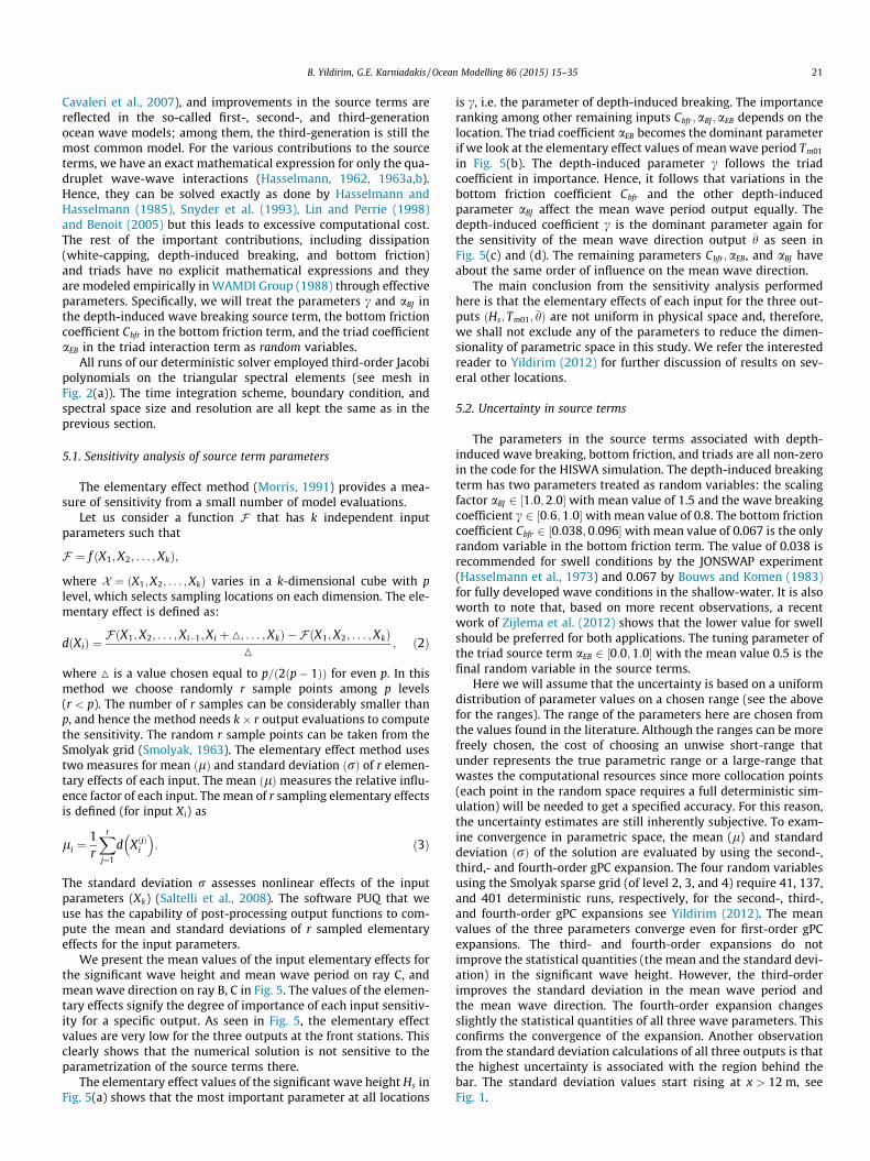
We present the mean values of the input elementary effects forthe significant wave height and mean wave period on ray C, andmean wave direction on ray B, C in Fig. 5. The values of the elemen-tary effects signify the degree of importance of each input sensitiv-ity for a specific output. As seen in Fig. 5, the elementary effectvalues are very low for the three outputs at the front stations. Thisclearly shows that the numerical solution is not sensitive to theparametrization of the source terms there.

The elementary effect values of the significant wave height Hs inFig. 5(a) shows that the most important parameter at all locations

is c, i.e. the parameter of depth-induced breaking. The importanceranking among other remaining inputs Cbfr ;aBJ;aEB depends on thelocation. The triad coefficient aEB becomes the dominant parameterif we look at the elementary effect values of mean wave period Tm01

in Fig. 5(b). The depth-induced parameter c follows the triadcoefficient in importance. Hence, it follows that variations in thebottom friction coefficient Cbfr and the other depth-inducedparameter aBJ affect the mean wave period output equally. Thedepth-induced coefficient c is the dominant parameter again forthe sensitivity of the mean wave direction output �h as seen inFig. 5(c) and (d). The remaining parameters Cbfr ;aEB, and aBJ haveabout the same order of influence on the mean wave direction.

The main conclusion from the sensitivity analysis performedhere is that the elementary effects of each input for the three out-puts ðHs; Tm01; �hÞ are not uniform in physical space and, therefore,we shall not exclude any of the parameters to reduce the dimen-sionality of parametric space in this study. We refer the interestedreader to Yildirim (2012) for further discussion of results on sev-eral other locations.

5.2. Uncertainty in source terms

The parameters in the source terms associated with depth-induced wave breaking, bottom friction, and triads are all non-zeroin the code for the HISWA simulation. The depth-induced breakingterm has two parameters treated as random variables: the scalingfactor aBJ 2 ½1:0;2:0� with mean value of 1.5 and the wave breakingcoefficient c 2 ½0:6;1:0�with mean value of 0.8. The bottom frictioncoefficient Cbfr 2 ½0:038;0:096�with mean value of 0.067 is the onlyrandom variable in the bottom friction term. The value of 0.038 isrecommended for swell conditions by the JONSWAP experiment(Hasselmann et al., 1973) and 0.067 by Bouws and Komen (1983)for fully developed wave conditions in the shallow-water. It is alsoworth to note that, based on more recent observations, a recentwork of Zijlema et al. (2012) shows that the lower value for swellshould be preferred for both applications. The tuning parameter ofthe triad source term aEB 2 ½0:0;1:0� with the mean value 0.5 is thefinal random variable in the source terms.

Here we will assume that the uncertainty is based on a uniformdistribution of parameter values on a chosen range (see the abovefor the ranges). The range of the parameters here are chosen fromthe values found in the literature. Although the ranges can be morefreely chosen, the cost of choosing an unwise short-range thatunder represents the true parametric range or a large-range thatwastes the computational resources since more collocation points(each point in the random space requires a full deterministic sim-ulation) will be needed to get a specified accuracy. For this reason,the uncertainty estimates are still inherently subjective. To exam-ine convergence in parametric space, the mean (l) and standarddeviation ðrÞ of the solution are evaluated by using the second-,third,- and fourth-order gPC expansion. The four random variablesusing the Smolyak sparse grid (of level 2, 3, and 4) require 41, 137,and 401 deterministic runs, respectively, for the second-, third-,and fourth-order gPC expansions see Yildirim (2012). The meanvalues of the three parameters converge even for first-order gPCexpansions. The third- and fourth-order expansions do notimprove the statistical quantities (the mean and the standard devi-ation) in the significant wave height. However, the third-orderimproves the standard deviation in the mean wave period andthe mean wave direction. The fourth-order expansion changesslightly the statistical quantities of all three wave parameters. Thisconfirms the convergence of the expansion. Another observationfrom the standard deviation calculations of all three outputs is thatthe highest uncertainty is associated with the region behind thebar. The standard deviation values start rising at x > 12 m, seeFig. 1.

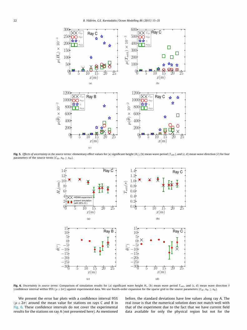
Fig. 5. Effects of uncertainty in the source terms: elementary effect values for (a) significant height (Hs), (b) mean wave period (Tm01), and (c, d) mean wave direction (�h) for fourparameters of the source terms (Cbfr ;aBJ ; c;aEB).

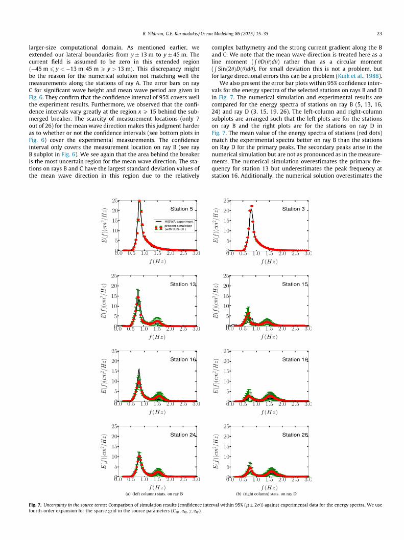
Fig. 6. Uncertainty in source terms: Comparison of simulation results for (a) significant wave height Hs , (b) mean wave period Tm01, and (c, d) mean wave direction �h(confidence interval within 95% (l� 2r)) against experimental data. We use fourth-order expansion for the sparse grid in the source parameters (Cbfr ;aBJ ; c;aBJ).

22 B. Yildirim, G.E. Karniadakis / Ocean Modelling 86 (2015) 15–35

We present the error bar plots with a confidence interval 95%ðl� 2rÞ around the mean value for stations on rays C and B inFig. 6. These confidence intervals do not cover the experimentalresults for the stations on ray A (not presented here). As mentioned

before, the standard deviations have low values along ray A. Thereal issue is that the numerical solution does not match well withthat of the experiment due to the fact that we have current fielddata available for only the physical region but not for the

B. Yildirim, G.E. Karniadakis / Ocean Modelling 86 (2015) 15–35 23

larger-size computational domain. As mentioned earlier, weextended our lateral boundaries from y� 13 m to y� 45 m. Thecurrent field is assumed to be zero in this extended regionð�45 m 6 y < �13 m; 45 m P y > 13 mÞ. This discrepancy mightbe the reason for the numerical solution not matching well themeasurements along the stations of ray A. The error bars on rayC for significant wave height and mean wave period are given inFig. 6. They confirm that the confidence interval of 95% covers wellthe experiment results. Furthermore, we observed that the confi-dence intervals vary greatly at the region x P 15 behind the sub-merged breaker. The scarcity of measurement locations (only 7out of 26) for the mean wave direction makes this judgment harderas to whether or not the confidence intervals (see bottom plots inFig. 6) cover the experimental measurements. The confidenceinterval only covers the measurement location on ray B (see rayB subplot in Fig. 6). We see again that the area behind the breakeris the most uncertain region for the mean wave direction. The sta-tions on rays B and C have the largest standard deviation values ofthe mean wave direction in this region due to the relatively

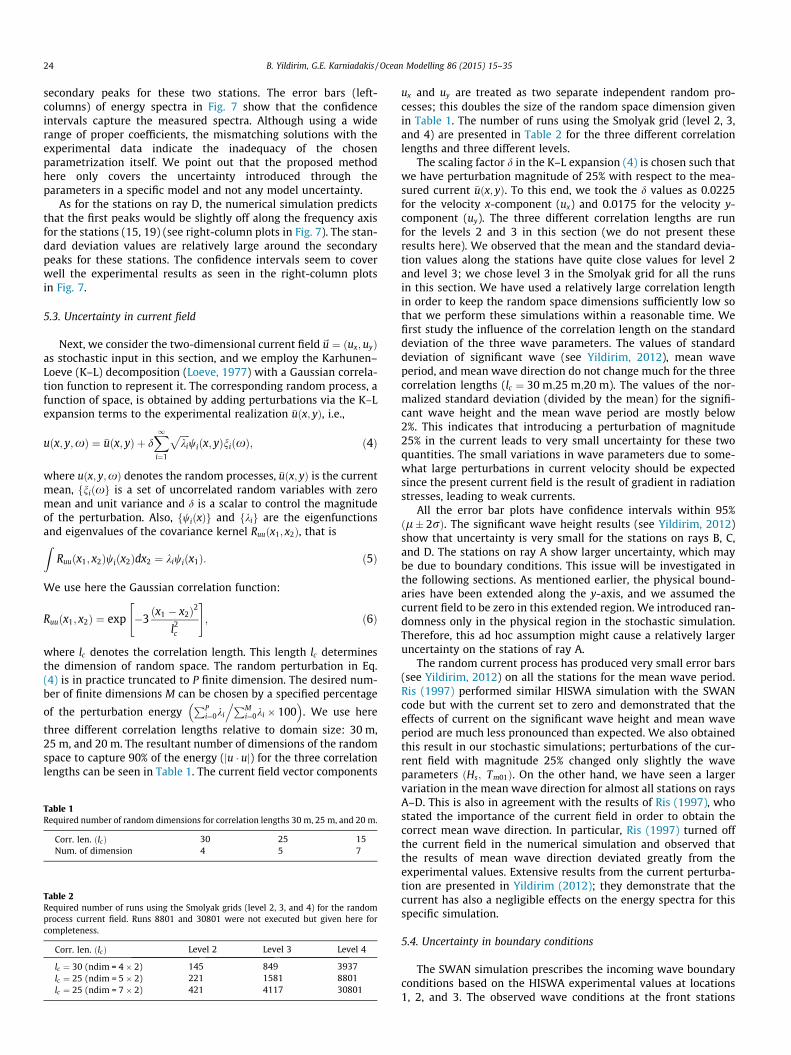
Fig. 7. Uncertainty in the source terms: Comparison of simulation results (confidence intefourth-order expansion for the sparse grid in the source parameters (Cbfr ;aBJ ; c;aBJ).

complex bathymetry and the strong current gradient along the Band C. We note that the mean wave direction is treated here as aline moment (

RhDðhÞdh) rather than as a circular moment

(R

Sinð2hÞDðhÞdh). For small deviation this is not a problem, butfor large directional errors this can be a problem (Kuik et al., 1988).

We also present the error bar plots within 95% confidence inter-vals for the energy spectra of the selected stations on rays B and Din Fig. 7. The numerical simulation and experimental results arecompared for the energy spectra of stations on ray B (5, 13, 16,24) and ray D (3, 15, 19, 26). The left-column and right-columnsubplots are arranged such that the left plots are for the stationson ray B and the right plots are for the stations on ray D inFig. 7. The mean value of the energy spectra of stations (red dots)match the experimental spectra better on ray B than the stationson Ray D for the primary peaks. The secondary peaks arise in thenumerical simulation but are not as pronounced as in the measure-ments. The numerical simulation overestimates the primary fre-quency for station 13 but underestimates the peak frequency atstation 16. Additionally, the numerical solution overestimates the

rval within 95% (l� 2r)) against experimental data for the energy spectra. We use

24 B. Yildirim, G.E. Karniadakis / Ocean Modelling 86 (2015) 15–35

secondary peaks for these two stations. The error bars (left-columns) of energy spectra in Fig. 7 show that the confidenceintervals capture the measured spectra. Although using a widerange of proper coefficients, the mismatching solutions with theexperimental data indicate the inadequacy of the chosenparametrization itself. We point out that the proposed methodhere only covers the uncertainty introduced through theparameters in a specific model and not any model uncertainty.

As for the stations on ray D, the numerical simulation predictsthat the first peaks would be slightly off along the frequency axisfor the stations (15, 19) (see right-column plots in Fig. 7). The stan-dard deviation values are relatively large around the secondarypeaks for these stations. The confidence intervals seem to coverwell the experimental results as seen in the right-column plotsin Fig. 7.

5.3. Uncertainty in current field

Next, we consider the two-dimensional current field~u ¼ ðux;uyÞas stochastic input in this section, and we employ the Karhunen–Loeve (K–L) decomposition (Loeve, 1977) with a Gaussian correla-tion function to represent it. The corresponding random process, afunction of space, is obtained by adding perturbations via the K–Lexpansion terms to the experimental realization �uðx; yÞ, i.e.,

uðx; y;xÞ ¼ �uðx; yÞ þ dX1i¼1

ffiffiffiffiki

pwiðx; yÞniðxÞ; ð4Þ

where uðx; y;xÞ denotes the random processes, �uðx; yÞ is the currentmean, fniðxg is a set of uncorrelated random variables with zeromean and unit variance and d is a scalar to control the magnitudeof the perturbation. Also, fwiðxÞg and fkig are the eigenfunctionsand eigenvalues of the covariance kernel Ruuðx1; x2Þ, that isZ

Ruuðx1; x2Þwiðx2Þdx2 ¼ kiwiðx1Þ: ð5Þ

We use here the Gaussian correlation function:

Ruuðx1; x2Þ ¼ exp �3ðx1 � x2Þ2

l2c

" #; ð6Þ

where lc denotes the correlation length. This length lc determinesthe dimension of random space. The random perturbation in Eq.(4) is in practice truncated to P finite dimension. The desired num-ber of finite dimensions M can be chosen by a specified percentage

of the perturbation energyPP

i¼0ki

.PMi¼0ki � 100

� �. We use here

three different correlation lengths relative to domain size: 30 m,25 m, and 20 m. The resultant number of dimensions of the randomspace to capture 90% of the energy (ju � uj) for the three correlationlengths can be seen in Table 1. The current field vector components

Table 1Required number of random dimensions for correlation lengths 30 m, 25 m, and 20 m.

Corr. len. ðlcÞ 30 25 15Num. of dimension 4 5 7

Table 2Required number of runs using the Smolyak grids (level 2, 3, and 4) for the randomprocess current field. Runs 8801 and 30801 were not executed but given here forcompleteness.

Corr. len. ðlcÞ Level 2 Level 3 Level 4

lc ¼ 30 (ndim = 4� 2) 145 849 3937lc ¼ 25 (ndim = 5� 2) 221 1581 8801lc ¼ 25 (ndim = 7� 2) 421 4117 30801

ux and uy are treated as two separate independent random pro-cesses; this doubles the size of the random space dimension givenin Table 1. The number of runs using the Smolyak grid (level 2, 3,and 4) are presented in Table 2 for the three different correlationlengths and three different levels.

The scaling factor d in the K–L expansion (4) is chosen such thatwe have perturbation magnitude of 25% with respect to the mea-sured current �uðx; yÞ. To this end, we took the d values as 0.0225for the velocity x-component (ux) and 0.0175 for the velocity y-component (uy). The three different correlation lengths are runfor the levels 2 and 3 in this section (we do not present theseresults here). We observed that the mean and the standard devia-tion values along the stations have quite close values for level 2and level 3; we chose level 3 in the Smolyak grid for all the runsin this section. We have used a relatively large correlation lengthin order to keep the random space dimensions sufficiently low sothat we perform these simulations within a reasonable time. Wefirst study the influence of the correlation length on the standarddeviation of the three wave parameters. The values of standarddeviation of significant wave (see Yildirim, 2012), mean waveperiod, and mean wave direction do not change much for the threecorrelation lengths (lc ¼ 30 m;25 m;20 m). The values of the nor-malized standard deviation (divided by the mean) for the signifi-cant wave height and the mean wave period are mostly below2%. This indicates that introducing a perturbation of magnitude25% in the current leads to very small uncertainty for these twoquantities. The small variations in wave parameters due to some-what large perturbations in current velocity should be expectedsince the present current field is the result of gradient in radiationstresses, leading to weak currents.

All the error bar plots have confidence intervals within 95%ðl� 2rÞ. The significant wave height results (see Yildirim, 2012)show that uncertainty is very small for the stations on rays B, C,and D. The stations on ray A show larger uncertainty, which maybe due to boundary conditions. This issue will be investigated inthe following sections. As mentioned earlier, the physical bound-aries have been extended along the y-axis, and we assumed thecurrent field to be zero in this extended region. We introduced ran-domness only in the physical region in the stochastic simulation.Therefore, this ad hoc assumption might cause a relatively largeruncertainty on the stations of ray A.

The random current process has produced very small error bars(see Yildirim, 2012) on all the stations for the mean wave period.Ris (1997) performed similar HISWA simulation with the SWANcode but with the current set to zero and demonstrated that theeffects of current on the significant wave height and mean waveperiod are much less pronounced than expected. We also obtainedthis result in our stochastic simulations; perturbations of the cur-rent field with magnitude 25% changed only slightly the waveparameters ðHs; Tm01Þ. On the other hand, we have seen a largervariation in the mean wave direction for almost all stations on raysA–D. This is also in agreement with the results of Ris (1997), whostated the importance of the current field in order to obtain thecorrect mean wave direction. In particular, Ris (1997) turned offthe current field in the numerical simulation and observed thatthe results of mean wave direction deviated greatly from theexperimental values. Extensive results from the current perturba-tion are presented in Yildirim (2012); they demonstrate that thecurrent has also a negligible effects on the energy spectra for thisspecific simulation.

5.4. Uncertainty in boundary conditions

The SWAN simulation prescribes the incoming wave boundaryconditions based on the HISWA experimental values at locations1, 2, and 3. The observed wave conditions at the front stations

B. Yildirim, G.E. Karniadakis / Ocean Modelling 86 (2015) 15–35 25

are not uniform while the mean wave directions for stations 1, 2,and 3 are �5:6�, 1:3�, and �3:6�, respectively. Similarly, the signif-icant wave heights observed on stations 1, 2, and 3 are 11.06 cm,10.33 cm, and 10.04 cm. We have neglected those variations onthe boundary so far and imposed the JONSWAP spectrum on theleft boundary condition with the peak frequency (f p0 ¼ 0:8 Hz)and the incoming wave direction (h0 ¼ �4:0�); the JONSWAP spec-trum is defined as

EJONSWAPðh; f Þ ¼ A1 cosmðh� h0ÞaPMg2ð2pÞ�4f�5 exp � 54

ff PM

� ��4� �

cexp �1

2

f=f p0�1l

� �2h i

; jh� h0j 6 90�;

0; jh� h0j > 90�;

8><>: ð7Þ

where c is a peak-enhancement factor and l is a controllingparameter of spectrum width, and A1 is defined asCðm=2þ 1Þ=½Cðmþ 1Þ=2Þ

ffiffiffiffipp� (m controls the width parameter in

a directional spectrum, see Holthuijsen (2007) for the details).The relevant parameter values for the JONSWAP spectrum usedhere are given in Section 4.1.

We consider non-uniform boundary conditions at the leftboundary modeled as random processes. To this end, we will takethe peak frequency f 0 and incoming wave direction h0 as the ran-dom processes and incorporate them into the left boundary. Weemploy the K–L decomposition of a Gaussian correlation functionto represent the random processes of the peak frequency f p0ðx; yÞand of incoming mean wave direction h0ðxL; yÞ. The random processof incoming peak frequency can be written as

f p0ðxL; y;xÞ ¼ �f p0ðxL; yÞ þ dX1i¼1

ffiffiffiffiki

pwiðxL; yÞniðxÞ; ð8Þ

where f p0ðxL; y;xÞ denotes random processes of incoming peak fre-quency and �f p0ðxL; yÞ is the incoming peak frequency mean. Theincoming peak frequency mean is taken as 0.8 Hz.

Similarly, we can write the K–L expansion for the incomingwave direction as

h0ðxL; y;xÞ ¼ �h0ðxL; yÞ þ dX1i¼1

ffiffiffiffiki

pwiðxL; yÞniðxÞ; ð9Þ

where h0ðxL; y;xÞ is random process of incoming wave directionand �h0ðxL; yÞ is incoming wave direction mean. The incoming wavedirection mean is assumed to be �4:0�. Here fnðxÞg is a set ofuncorrelated random variables, and fwiðxÞg and fkig are the eigen-functions and eigenvalues of the covariance kernel Rbbðx1; x2Þ, that isZ

Rbbðx1; x2Þwiðx2Þdx2 ¼ kiwiðx1Þ: ð10Þ

We use here the Gaussian correlation function:

Rbbðx1; x2Þ ¼ exp �3ðx1 � x2Þ2

l2c

" #; ð11Þ

where lc denotes the correlation length. Note that Rbb is defined onlyfor the left boundary (½xL ¼ 0; y ¼ ð�45;45Þ�). The random processesare introduced to the computational grid nodes at the left boundary.The boundary condition in our high-order ocean wave code is line-arly interpolated to the Gauss–Lobatto quadrature points of bound-ary face from these grid nodes. The correlation length lc determinesthe dimension of random space, here we set it to 15 m, i.e., equal totriangle edge length on the boundary side. The dimension of theabove covariance kernel in this case is the number of left boundarygrid nodes, which is seven. The resulting dimension of the random

space capturing 100% of the energy (see Section 5.3) for this corre-lation length is seven for each random process. The total dimensionof the random space will be 14 accounting for both processes.

The perturbation scale is d in the K–L expansions in Eqs. (8) and(9) based on the variation of mean wave direction and significantwave heights of experiment at the sites 1, 2, and 3. The mean wavedirection is chosen as �4�, which is equal to the average observa-tional values between site 1 (�5:6�) and 3 (�3:6�); site 2 has an

observational value of 1:3�. The perturbation scale for the meanwave direction is chosen as 5.0 so that the perturbation liesbetween �8� and 2�. As for peak frequency random process, theperturbation scale is taken as 0.08 to have a variation correspond-ing to perturbation of 10%; this is based on the variation ofobserved significant wave heights at sites 1, 2, and 3, which arerespectively 11.06 cm, 10.33 cm, and 10.04 cm.

The mean and the standard deviations are well converged forlevel 2 and level 3 gPC expansions. We chose level 3 for theSmolyak grid for this section. The dimension of random spacewill be 14 for level 3 expansion, which requires 4117 determin-istic runs.

We present the error bar plots (only on ray B and C) for thethree statistical wave parameters (Hs; Tm01; �h) in Fig. 8. All the errorbar plots shown here have confidence intervals within 95%(l� 2r). The first important observation is that we have largeruncertainties at the locations before the breaker than we observeddue to the uncertainty in the source term parametrization for thesignificant wave height parameter (see plots (a) in Figs. 8 and 6).The significant wave height error bars are smaller at the locationsstationed behind the submerged breaker (x > 15 m). Since depth-breaking is the dominant process in the HISWA experiment, it isnot surprising to see that variations in the boundary have beendamped across the submerged bar. For ray A, which is not affectedso much from the changing bathymetry, there is large variationeverywhere (results not shown here, see Yildirim (2012)). The ran-dom boundary conditions strongly affect the mean wave periodresults as seen in Fig. 8(b). We have treated the incoming meanwave direction also as a random process. Accordingly, we see largevariation about the mean around the ray B and C stations inFig. 8(c) and (d); the variations are increased after the submergedbreaker. We observe large variations around the front stations,which were not observed due to uncertainties in source termsand current field.

5.5. Uncertainty of source and boundary condition

Next we study the combined effect of randomness in the sourceterms and boundary conditions. The four random variables of thesource terms (aBJ; c;Cbr , and aEB) follow a uniform probability dis-tribution within the range specified in Section 5.2. The dimensionof random space is the sum of 14 random variables from the K–Lexpansions of the random processes of the incoming peak andwave direction (see Eqs. (8) and (9)) and the four random variablesin the source parametrization. The total number of deterministicruns for level 3 and the eighteen variables is 8509. Our resultsare presented in Figs. 9–11. The experimental values of significantwave height are all contained within 95% confidence interval alongthe rays A–D as seen in Fig. 9. The confidence intervals are signif-icantly modified for the stations along ray A and the front stations

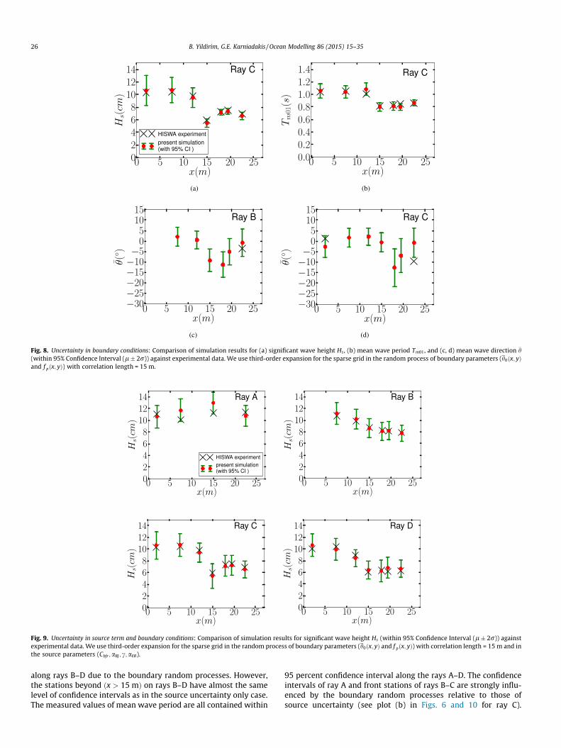
Fig. 8. Uncertainty in boundary conditions: Comparison of simulation results for (a) significant wave height Hs , (b) mean wave period Tm01, and (c, d) mean wave direction �h(within 95% Confidence Interval (l� 2r)) against experimental data. We use third-order expansion for the sparse grid in the random process of boundary parameters (h0ðx; yÞand f pðx; yÞ) with correlation length = 15 m.

Fig. 9. Uncertainty in source term and boundary conditions: Comparison of simulation results for significant wave height Hs (within 95% Confidence Interval (l� 2r)) againstexperimental data. We use third-order expansion for the sparse grid in the random process of boundary parameters (h0ðx; yÞ and f pðx; yÞ) with correlation length = 15 m and inthe source parameters (Cbfr ;aBJ ; c;aEB).

26 B. Yildirim, G.E. Karniadakis / Ocean Modelling 86 (2015) 15–35

along rays B–D due to the boundary random processes. However,the stations beyond ðx > 15 mÞ on rays B–D have almost the samelevel of confidence intervals as in the source uncertainty only case.The measured values of mean wave period are all contained within

95 percent confidence interval along the rays A–D. The confidenceintervals of ray A and front stations of rays B–C are strongly influ-enced by the boundary random processes relative to those ofsource uncertainty (see plot (b) in Figs. 6 and 10 for ray C).

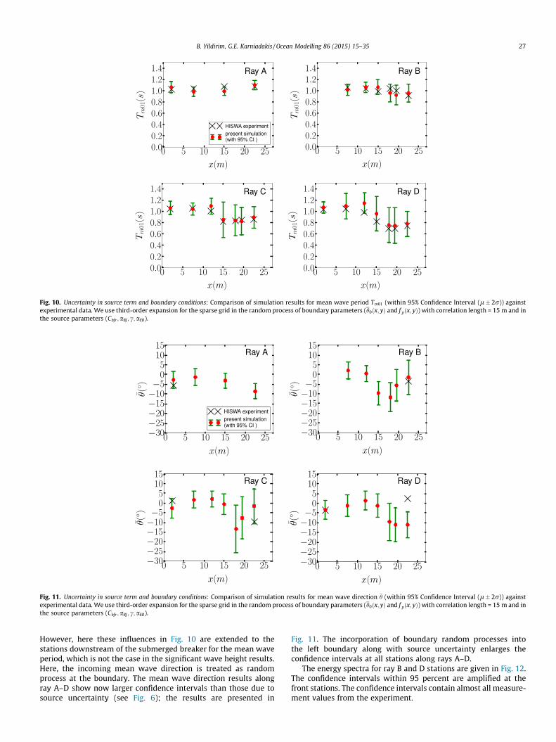
Fig. 10. Uncertainty in source term and boundary conditions: Comparison of simulation results for mean wave period Tm01 (within 95% Confidence Interval (l� 2r)) againstexperimental data. We use third-order expansion for the sparse grid in the random process of boundary parameters (h0ðx; yÞ and f pðx; yÞ) with correlation length = 15 m and inthe source parameters (Cbfr ;aBJ ; c;aEB).

Fig. 11. Uncertainty in source term and boundary conditions: Comparison of simulation results for mean wave direction �h (within 95% Confidence Interval (l� 2r)) againstexperimental data. We use third-order expansion for the sparse grid in the random process of boundary parameters (h0ðx; yÞ and f pðx; yÞ) with correlation length = 15 m and inthe source parameters (Cbfr ;aBJ ; c;aEB).

B. Yildirim, G.E. Karniadakis / Ocean Modelling 86 (2015) 15–35 27

However, here these influences in Fig. 10 are extended to thestations downstream of the submerged breaker for the mean waveperiod, which is not the case in the significant wave height results.Here, the incoming mean wave direction is treated as randomprocess at the boundary. The mean wave direction results alongray A–D show now larger confidence intervals than those due tosource uncertainty (see Fig. 6); the results are presented in

Fig. 11. The incorporation of boundary random processes intothe left boundary along with source uncertainty enlarges theconfidence intervals at all stations along rays A–D.

The energy spectra for ray B and D stations are given in Fig. 12.The confidence intervals within 95 percent are amplified at thefront stations. The confidence intervals contain almost all measure-ment values from the experiment.

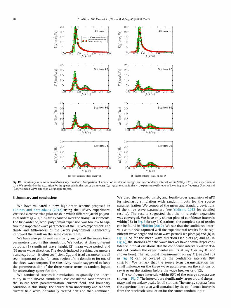
Fig. 12. Uncertainty in source term and boundary conditions: Comparison of simulation results for energy spectra (confidence interval within 95% (l� 2r)) and experimentaldata. We use third-order expansion for the sparse grid in the source parameters (Cbfr ;aBJ ; c;aBJ) and in the K–L expansion coefficients of incoming peak frequency (f pðx; yÞ) and(h0ðx; yÞ) mean wave direction as random process.

28 B. Yildirim, G.E. Karniadakis / Ocean Modelling 86 (2015) 15–35

6. Summary and conclusions

We have validated a new high-order scheme proposed inYildirim and Karniadakis (2012) using the HISWA experiment.We used a coarse triangular mesh in which different Jacobi polyno-mial orders ðp ¼ 1;3;5Þ are expanded over the triangular elements.The first-order of Jacobi polynomial expansion was too low to cap-ture the important wave parameters of the HISWA experiment. Thethird- and fifth-orders of the Jacobi polynomials significantlyimproved the result on the same coarse mesh.

We have also performed sensitivity analysis of the source termparameters used in this simulation. We looked at three differentoutputs: (1) significant wave height, (2) mean wave period, and(3) mean wave direction. The depth-induced breaking parametersc and aBJ , bottom friction coefficient Cbfr , and triad parameter aEB allseem important either for some region of the domain or for one ofthe three wave outputs. The sensitivity results suggested to keepthe parametrization of the three source terms as random inputsfor uncertainty quantification.

We conducted stochastic simulations to quantify the uncer-tainty in the HISWA simulation. We considered randomness inthe source term parametrization, current field, and boundarycondition in this study. The source term uncertainty and randomcurrent field were individually treated first and then combined.

We used the second-, third-, and fourth-order expansion of gPCfor stochastic simulation with random inputs for the sourceparametrization. We compared the mean and standard deviationsof the three wave parameters (see Yildirim, 2012 for detailedresults). The results suggested that the third-order expansionwas converged. We have only shown plots of confidence intervalswithin 95% in Fig. 6 for ray B, C stations; the complete set of resultscan be found in Yildirim (2012). We see that the confidence inter-vals within 95% captured well the experimental results for the sig-nificant wave height and mean wave period (see plots (a) and (b) inFig. 6). As for the mean wave direction (see plots (c) and (d) inFig. 6), the stations after the wave breaker have shown larger con-fidence interval variations. But the confidence intervals within 95%did not contain the experimental results at ray C or ray D (notshown here). The rightmost measurement on ray C (see plot (d)in Fig. 6) can be covered by the confidence intervals 99%ðl� 3rÞ. We remark that the source term parametrization hassmall influence on the three wave parameters on the stations ofray A or on the stations before the wave breaker ðx < 12Þ.

The confidence intervals within 95% of the energy spectra areshown in Fig. 7. The intervals are significantly larger around the pri-mary and secondary peaks for all stations. The energy spectra fromthe experiment are also well contained by the confidence intervalsfrom the stochastic simulation for the source random input.

B. Yildirim, G.E. Karniadakis / Ocean Modelling 86 (2015) 15–35 29

The current field has a direct influence on depth-induced andcurrent-induced wave refraction and shoaling. We introduced arandom current field by using the Karhunen–Loeve expansion ofthe exponential Gaussian correlation function. The correlationlength determines the dimension of random space. We have testedthree different correlation lengths: 30 m, 25 m, and 20 m; theseresults are not presented here but they can be found in Yildirim(2012). We briefly mention that the standard deviation of the threeimportant wave parameters ðHs; Tm01; �hÞ did not make a signifi-cant difference between level 3 and level 4 expansion from theSmolyak grid. We chose the correlation length as 25 m and usedthe level 3 from the Smolyak grid for stochastic simulation of therandom current input. Perturbations with magnitude of about25% were introduced to x and y velocity components of the exper-imental current field. Although it is a relatively large perturbationof the current field, the confidence intervals (see the results inYildirim (2012)) did not induce any noticeable differences in thesignificant wave height or the mean wave period.

The error bars of energy spectra were slightly changed aroundthe primary peaks at the stations (see detailed results in Yildirim(2012)) where strong current gradients were present. For this per-turbation level, the uncertainty of source term parametrization stillhas a much larger effect than the random current field input on thewave parameters and energy spectra.

The incoming wave direction and peak frequency at the leftboundary were treated as random processes. The error bar plotsare presented for the three important integrated parameters inFig. 8. An important observation is that we see larger variationaround ray A stations and the front stations of ray B–D for the inte-grated parameters (only ray C and B results are presented here).The variations are relatively smaller toward the downstream sta-tions for the significant wave height and mean wave periods. How-ever, we see larger error bars on the downstream stations for themean wave direction.

We also performed stochastic simulations by considering com-bined sources of uncertainty. First we combined two randomsources (source and current) to perform a stochastic simulation.The resulted error plots (not shown here) reflect the same levelof uncertainty as the one resulted from parametrization of thesource only. This, in turn, implies the dominance of the uncertaintyfrom the source terms. Adding to the uncertainty from boundaryconditions to both fields (source and current) will increase thedimension of the random space on a level that we cannot affordthe computational cost. Since the uncertainty of the current fieldbarely changes the overall outcome, the relevant statistics for theintegrated wave parameters can be obtained by dropping theuncertainty of the current field and combining two random sourcesfrom the source term parametrization and boundary condition.Hence, such stochastic simulation will yield the combined uncer-tainty from all the inputs (source terms, current field, and bound-ary condition). The error bars with confidence intervals within 95%are shown in Figs. 9–11. The confidence intervals covered well theobservational values from the experiment except the value on theexperimental station of ray D for the mean wave direction. Fig. 12shows that the confidence intervals contained well the experimen-tal measurements for the energy spectra for the probe stations.Wherever a large variation of the confidence intervals occurs (suchas around the first and secondary peaks) it signifies the sensitivityof a solution to the input parameters.

Acknowledgments

This work was supported by the MIT Sea Grant Program and byDOE. The authors would like to thank Dr. N. Booij (Digital Hydrau-lics Holland) for providing the experimental data to us and to theanonymous reviewers for providing the SWAN simulation data

and their valuable comments and suggestions to improve the qual-ity of the paper.

Appendix A. Source terms

A.1. Triad wave-wave interactions (Snl3)

The Lumped Triad Approximation (LTA) by Eldeberky (1996) isthe simplest expression for triad wave interactions. The approxi-mation is

Snl3ðh;rÞ ¼ S�nl3ðh;rÞ þ Sþnl3ðh;rÞ; ðA:1Þ

and the positive term contribution is computed as

Sþnl3 ¼max 0;aEB2pccgJ2j sin bj E2ðh;r=2Þ � 2Eðh;r=2ÞEðh;rÞn oh i

;

ðA:2Þ

where aEB is a control parameter. The negative contribution ofsource terms can be defined in terms of the positive one as

S�nl3 ¼ �2Sþnl3ðh;2rÞ: ðA:3Þ

The bi-phase parameter b is approximated by using the Ursell num-ber Ur:

b ¼ �p2þ p

2tanh

0:2Ur

; ðA:4Þ

and

Ur ¼ g

8ffiffiffi2p

p2

HsT2m01

d2 : ðA:5Þ

The coefficient J (Madsen and Sørenson, 1993) can now be definedas

J ¼k2r=2 gdþ 2c2

r=2

� �krd gdþ 2

15 gd3k2r � 2

5 r2d2� � : ðA:6Þ

A.2. Depth-induced wave breaking (Sbr)

The mean rate of energy dissipation due to depth-inducedbreaking is:

Dtot ¼ �14aBJQ b

~r2p

H2

max; ðA:7Þ

where the value of aBJ is of the order of one. The fraction of breakingwaves is represented by Qb, which is derived by assuming cumula-tive probability distributions of all waves (Battjes and Janssen,1978; Battjes and Stive, 1985) from the following relation:

1� Q b

log Qb¼ �8

Hrms

H2max

; ðA:8Þ

where Hrms is the root-mean-square of wave height and Hmax is themaximum wave height for a given depth. The maximum waveheight is defined as Hmax ¼ cd. The breaker parameter c is chosenas an default average value of 0.73 from the work of Battjes andStive (1985).

The depth-induced wave breaking source term (Eldeberky,1996) can be modeled as

Sbrðh;rÞ ¼Dtot

EtotEðh;rÞ: ðA:9Þ

Note that Sbr will have a negative sign due to Dtot .

30 B. Yildirim, G.E. Karniadakis / Ocean Modelling 86 (2015) 15–35

A.3. Bottom friction (Sbfr)

Bottom friction is modeled from WAMDI Group (1988) based onfurther simplification of the bottom friction model of the JONSWAPexperiment (Hasselmann et al., 1973) as

Sbfrðh;rÞ ¼ �Cbfrr2

g2sinh2ðkdÞEðh;rÞ; ðA:10Þ

where Cbfr is the tunable bottom friction coefficient. The modelingof the bottom friction source term assumes that the tangentialstress on the bottom can be modeled by a quadratic friction law(Hasselmann and Collins, 1968), which can be interpreted in termsof the bottom friction source term, leading to the above formulation(Hasselmann et al., 1973). In the JONSWAP experiment(Hasselmann et al., 1973) 10 swell cases were tested and showingthat the bottom friction coefficient changes from 0.03 to 0.16, witha mean value of 0:038 m2 s�3. The bottom friction coefficientCbfr ¼ 0:067 m2 s�3 has been used by Bouws and Komen (1983)for fully developed waves in shallow water. The coefficient Cbfr isnot constant but depends on the bottom amplitude Reynolds num-ber and the bed roughness. We refer the interested readers toYoung’s book (Young, 1999) for further discussion and references.

Appendix B. Numerical discretization

We presented a detailed description of numerical discretizationof phased-averaged ocean wave equation in our previous work(Yildirim and Karniadakis, 2012; Yildirim, 2012), which will besummarized in this section. Let us now define the following fluxeswith the transformation of the frequency coordinate r! f

¼ p 2ðr�rminÞrmax�rmin

� 1h i

:

E ¼ cxNðf; h; x; y; tÞ; F ¼ cyNðf; h; x; y; tÞ; G ¼ chNðf; h; x; y; tÞ;H ¼ cfNðf; h; x; y; tÞ:

Using the above definitions, the action balance equation in fluxform is written as

@N@tþ @E@xþ @F@yþ @G@hþ Jfr

@H@f¼ S

r; ðB:1Þ

where Jfr ¼ 2p=ðrmax � rminÞ.

B.1. Fourier-collocation methods for the spectral derivatives

We use Fourier-collocation in a directional domain extendingfrom�p to p due to periodicity. The frequency direction ðrÞ is usu-ally a truncated domain, which is non-periodic. This, in turn, makesa standard Fourier-collocation along the frequency direction apply-ing impossible. The numerical solution passing the boundariesshould not be reflected by the truncated ends to a computationaldomain. A modification to apply the standard Fourier-collocationfor the derivative term along the frequency axis, using absorbingboundary layer approach (If et al., 1987), was proposed in our pre-vious work (Yildirim and Karniadakis, 2012), and it will bedescribed in Appendix B.3. Let us discretize the wave direction hand the transformed frequency direction ðfÞ as

hk ¼ �pþ 2pN

k 8k 2 ½0;1; . . . ;N � 1�;

fl ¼ �pþ 2pN

l 8l 2 ½0;1; . . . ;N � 1�;

and then using Lagrangian interpolation (Gottlieb and Orszag, 1977;Hesthaven et al., 2007), we can compute

@G@h

����h¼hk

¼XN�1

j¼0

DkjGðf; hj; x; y; tÞ; ðB:2Þ

where Dkj is the differentiation matrix for Fourier-collocation. Sim-ilarly, we obtain

@H@f

����f¼fl

¼XN�1

j¼0

DljHðfj; h; x; y; tÞ: ðB:3Þ

The differentiation matrix (Hesthaven et al., 2007) for an even num-ber of collocation points (Lagrangian polynomial if q ¼ 0) reads in adummy coordinate z (either h or f to obtain the above fluxderivatives)

Dqij ¼

2N

XN=2

n¼0

1cn

ðinÞq cos½nðzi � zjÞ�; q eveniðinÞq sin½nðzi � zjÞ�; q odd

(ðB:4Þ

where c0 ¼ cN=2 ¼ 2 and cn ¼ 1, otherwise. For an odd number ofcollocation points, the same differentiation matrix can be used bysetting cn ¼ 1 for all values of n.

B.2. Mapping in the spectral direction

The standard Fourier-collocation employs equi-spaced distribu-tion in the directional domain. The number of collocation pointscan be so large in case of a steep solution localized in a specificregion. While resolving the steep solution, one will over-resolvethe smoother part of the solution, wasting the computationalresources. Alternatively, we can define a mapping to cluster theFourier-collocation points around a specified region (local refine-ment). This clustering can be achieved by employing a mappingfor a specified region.

The atan mapping (Boyd, 1987, 2001) can be defined in ½�p;p�for the spectral direction

h ¼ gðv; LÞ ¼ 2 arctan½L tanð0:5vÞ� þ v0; ðB:5Þ

where v denotes computational space which permits the standardFourier-collocation method for differentiation, and the constantparameter L controls the amount of clustering around the peak cen-ter v0. Using a change of derivative coordinate transformation forthe mapping relation in Eq. (B.5), we obtain a new differentiationmatrix and compute the spectral direction derivatives with them(Yildirim and Karniadakis, 2012; Yildirim, 2012).

We have found that this mapping can save us up to eight timesin the number of collocation points in the directional domain. Thederivation of new differentiation matrix and the demonstration ofcomputational savings for a narrow directional spectrum was dis-cussed in our previous work (Yildirim and Karniadakis, 2012;Yildirim, 2012).

B.3. Absorbing boundary treatment in frequency direction

The true boundary conditions for a truncated domain permitincoming waves without any reflection back to the computationaldomain. For the frequency direction, we have used the AbsorbingBoundary Layer (ABL) approach (If et al., 1987) to satisfy non-reflective boundary conditions; this effectively enforces periodicityat the truncated domain boundaries.

To impose the ABL approach, we add the term gðrÞ Nðh; x; y; tÞto the original equation Eq. (1), and hence the new modified actionbalance equation is

@Nðh;r; x; y; tÞ@t

þ @cg;xNðh;r; x; y; tÞ@x

þ @cg;yNðh;r; x; y; tÞ@y

þ @chNðh;r; x; y; tÞ@h

þ @crNðh;r; x; y; tÞ@r

þ gðrÞ � Nðh;r; x; y; tÞ|fflfflfflfflfflfflfflfflfflfflfflfflfflfflfflfflffl{zfflfflfflfflfflfflfflfflfflfflfflfflfflfflfflfflffl}modificationterm

¼ Sðr; h; x; y; tÞr

; ðB:6Þ

B. Yildirim, G.E. Karniadakis / Ocean Modelling 86 (2015) 15–35 31

where gðrÞ is the absorbing function, achieving zero values insidethe domain and non-zero values in the absorbing layers, dampingthe numerical solution in these regions. The absorbing functioncan be defined in the computational domain f in ½�p;p� as follows:

gðfÞ ¼ cL 1 � tanh½aLðfþ pÞ�ð Þ þ cR 1 þ tanh½aRðf� pÞ�ð Þ; ðB:7Þ

where c controls the magnitude of the absorbing functions, a deter-mines the effective width of the absorbing layers, and L and Rdenote the left and right layers. The parameter couples aL and aR

control the ABL widths. We refer the interested readers for thedetails of the parameters to our previous work (Yildirim andKarniadakis, 2012; Yildirim, 2012).

Using the collocation differentiation Eqs. (B.2) and (B.3) in theflux form of action Eq. (B.1) with the above modification term,we can define the term L as

Lðhk; fl; x; y; tÞ ¼@G@h

����h¼hk

þ Jfr@H@f

����f¼fl

þ gðrlÞNðhk;rl; x; y; tÞ

� Sðhl;rk; x; y; tÞ: ðB:8ÞWith the above definition, the flux form equation is written as@N@tþ @E@xþ @F@yþ Lðhk; fl; x; y; tÞ ¼ 0; ðB:9Þ

B.4. Spatial discretizations

We will use discontinuous Galerkin (DG) (Hesthaven andWarburton, 2007; Hesthaven et al., 2007; Karniadakis andSherwin, 1999) spectral element discretization for the geographi-cal space. The discontinuous Galerkin formulation can be statedas: Find an approximate solution Nh in the piece-wise polynomialspace VhðXÞ, defined as VhðXÞ 2 PkðXÞ

� �where PkðXÞ denotes the col-

lection of polynomials of degree up to k in the element X such thatZX

@Nh

@tvhdXþ

ZX

@Eh

@xvhdXþ

ZX

@Fh

@yvhdX

þZ

XLðhk; fl; x; y; tÞvhdX ¼ 0; 8vh 2 Vh; ðB:10Þ

where X is an arbitrary triangle element, and L in Eq. (B.8) is sumof spectral space derivatives, the modification term, and physicalsource terms which is defined above. Applying integration by parts,we obtainZ

X

@Nh

@tvhdX�

ZX

Eh@vh

@xdX�

ZX

Fh@vh

@ydXþ

Z@X

Ehvh � ndS

þZ@X

Fhvh � ndSþZ

XLðhk; fl; x; y; tÞvhdX ¼ 0: ðB:11Þ

To compute the above integrals on the standard triangle, we trans-form an arbitrary triangle domain X to a standard triangle(�1 6 n1 þ n2 6 1). To define orthogonal coordinates, we introducea collapsed coordinate transformation that allows us to constructtwo-dimensional expansion functions for a triangle region the sameas in a structured region. The collapsed transformation is defined asKarniadakis and Sherwin (1999)

g1 ¼2ð1þ n1Þ

1� n2� 1; g2 ¼ n2; ðB:12Þ

where g1 and g2 are new coordinates �1 6 g1;g2 6 1, see Fig. B.13,removing coordinate dependency of bounds in a triangle domain(�1 6 n1 þ n2 6 1) – see Yildirim and Karniadakis (2012) andYildirim (2012) for the details of the transformation and the finalform of the equation.

Seeking approximate solution Nh expanded by orthogonalexpansional functions and choosing test function vh as the sameorthogonal expansion functions (Galerkin projection) such as

Nh ¼XP1

p¼0

XP2

q¼0

upqðtÞwpðg1Þwpqðg2Þ and ðB:13aÞ

vh ¼ wmðg1Þwmnðg2Þ; ðB:13bÞ

the complete polynomial space for a triangular region can be con-structed fðpqÞj0 6 p; q; p 6 P1; pþ q 6 P2; P1 6 P2g. The orthogonalexpansion functions in terms of Jacobi polynomials are defined inKarniadakis and Sherwin (1999):

wpðg1Þ ¼ P0;0p ðg1Þ; wmðg1Þ ¼ P0;0

m ðg1Þ;

wpqðg2Þ ¼1� g2

2

p

P2pþ1;0q ðg2Þ; wmnðg2Þ ¼

1� g2

2

m

P2mþ1;0n ðg2Þ:

ðB:14Þ

Inserting the approximate solution Nh (Nh 2 Vh) and test function vh

into the transformed form of Eq. (B.11) – now casted in transformedcoordinates g1 and g2 – using Jacobi polynomials wp and wpq definedin Eq. (B.14), we will obtain the final approximated equation (seeYildirim and Karniadakis, 2012; Yildirim, 2012). We choice theupwind flux (see the other numerical flux options from Toro(1999)) to replace the boundary flux terms in Eq. (B.11).

B.5. Numerical integration of spatial and spectral terms

The discretized equations will be now reduced to an ordinarydifferential equation (ODE) for the expansion coefficients upq

Mpq;pqdupqðtÞ

dt¼ 1

Jxn

Spq þ Tpq � Epq � Fpq � Lpq� �

; ðB:15Þ

where the mass matrix M, the stiffness vectors S and T, the edgefluxes E and F, and numerical source term L are, respectively, theresult of integrated terms in the approximate final equation. Notethat the approximate equation is derived after applying the twotransformations, and replacing N with Nh and v with vh in Eq.(B.11) (see Yildirim and Karniadakis, 2012; Yildirim, 2012 for thedetails).

The mass matrix M is the result of the following quadratureintegration of the time term by using the orthogonality of Jacobipolynomials

RPmðxÞPnðxÞdx ¼ 0; m – n

� �:

Mpq;pq ¼2

ð1þ 2pÞð1þ pþ qÞ : ðB:16Þ

The one great advantage of using orthogonal polynomials is that theinversion of mass matrix is trivial since it is diagonal. The remainingintegration terms (S;T;E, and F; L) need to be numerically com-puted. The details can be found in our previous work (Yildirimand Karniadakis, 2012; Yildirim, 2012). In summary, we use mixedGauss–Lobatto/Gauss–Radau quadrature to compute each integra-tion term.

B.6. Numerical time discretization

With regards to temporal discretization, we employed second-and third-order (Gottlieb and Shu, 1998), as well as the fourth-order explicit (5-stages) (Spiteri and Steven, 2001) Strong StabilityPreserving Runge–Kutta (SSP-RK) schemes. The 2nd order SSP-RKschemes used in the entire study Gottlieb and Shu (1998) andHesthaven and Warburton (2007)

v ð1Þ ¼ un þ Mt rðun; tnÞ;

unþ1 ¼ 12

un þ v ð1Þ þ Mt rðv ð1Þ; tn þ Mt� �

; ðB:17Þ

where r is the right-hand side of Eq. (B.15), and Mt is the time stepsize.

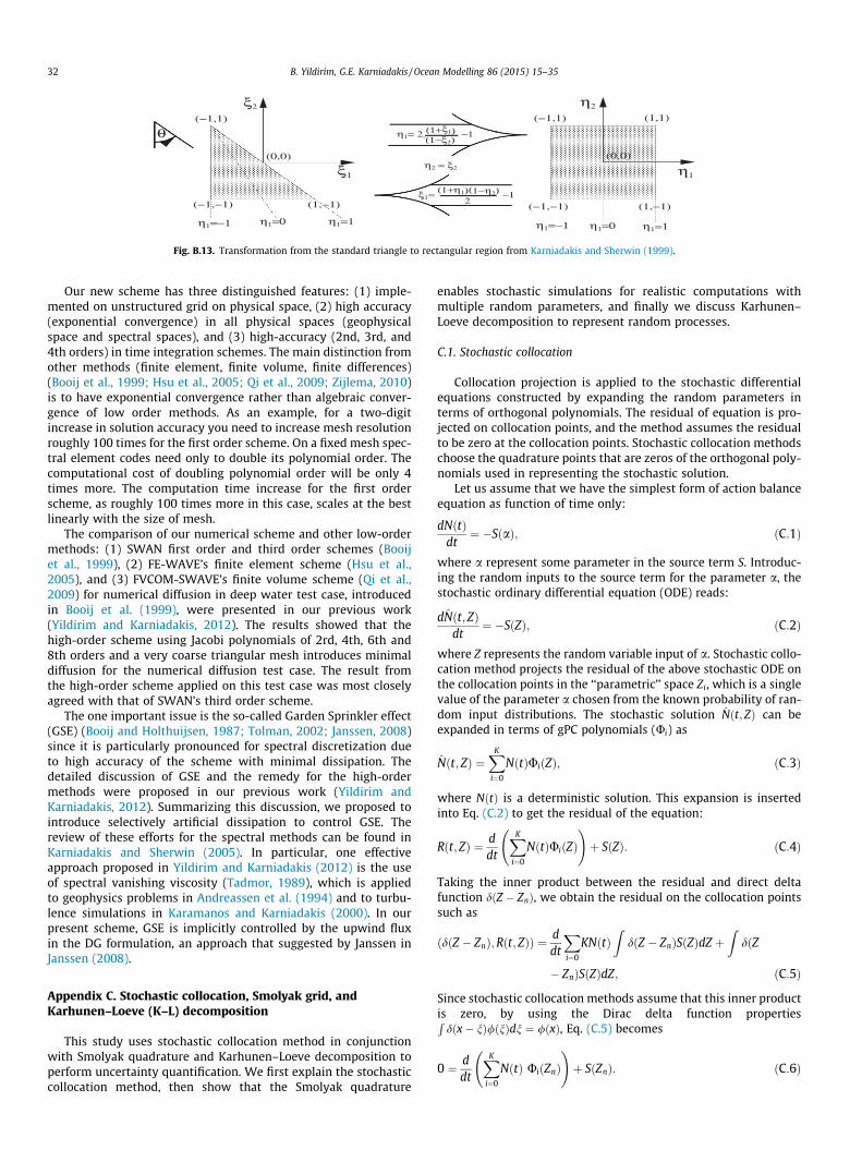
Fig. B.13. Transformation from the standard triangle to rectangular region from Karniadakis and Sherwin (1999).

32 B. Yildirim, G.E. Karniadakis / Ocean Modelling 86 (2015) 15–35

Our new scheme has three distinguished features: (1) imple-mented on unstructured grid on physical space, (2) high accuracy(exponential convergence) in all physical spaces (geophysicalspace and spectral spaces), and (3) high-accuracy (2nd, 3rd, and4th orders) in time integration schemes. The main distinction fromother methods (finite element, finite volume, finite differences)(Booij et al., 1999; Hsu et al., 2005; Qi et al., 2009; Zijlema, 2010)is to have exponential convergence rather than algebraic conver-gence of low order methods. As an example, for a two-digitincrease in solution accuracy you need to increase mesh resolutionroughly 100 times for the first order scheme. On a fixed mesh spec-tral element codes need only to double its polynomial order. Thecomputational cost of doubling polynomial order will be only 4times more. The computation time increase for the first orderscheme, as roughly 100 times more in this case, scales at the bestlinearly with the size of mesh.

The comparison of our numerical scheme and other low-ordermethods: (1) SWAN first order and third order schemes (Booijet al., 1999), (2) FE-WAVE’s finite element scheme (Hsu et al.,2005), and (3) FVCOM-SWAVE’s finite volume scheme (Qi et al.,2009) for numerical diffusion in deep water test case, introducedin Booij et al. (1999), were presented in our previous work(Yildirim and Karniadakis, 2012). The results showed that thehigh-order scheme using Jacobi polynomials of 2rd, 4th, 6th and8th orders and a very coarse triangular mesh introduces minimaldiffusion for the numerical diffusion test case. The result fromthe high-order scheme applied on this test case was most closelyagreed with that of SWAN’s third order scheme.

The one important issue is the so-called Garden Sprinkler effect(GSE) (Booij and Holthuijsen, 1987; Tolman, 2002; Janssen, 2008)since it is particularly pronounced for spectral discretization dueto high accuracy of the scheme with minimal dissipation. Thedetailed discussion of GSE and the remedy for the high-ordermethods were proposed in our previous work (Yildirim andKarniadakis, 2012). Summarizing this discussion, we proposed tointroduce selectively artificial dissipation to control GSE. Thereview of these efforts for the spectral methods can be found inKarniadakis and Sherwin (2005). In particular, one effectiveapproach proposed in Yildirim and Karniadakis (2012) is the useof spectral vanishing viscosity (Tadmor, 1989), which is appliedto geophysics problems in Andreassen et al. (1994) and to turbu-lence simulations in Karamanos and Karniadakis (2000). In ourpresent scheme, GSE is implicitly controlled by the upwind fluxin the DG formulation, an approach that suggested by Janssen inJanssen (2008).

Appendix C. Stochastic collocation, Smolyak grid, andKarhunen–Loeve (K–L) decomposition

This study uses stochastic collocation method in conjunctionwith Smolyak quadrature and Karhunen–Loeve decomposition toperform uncertainty quantification. We first explain the stochasticcollocation method, then show that the Smolyak quadrature

enables stochastic simulations for realistic computations withmultiple random parameters, and finally we discuss Karhunen–Loeve decomposition to represent random processes.

C.1. Stochastic collocation

Collocation projection is applied to the stochastic differentialequations constructed by expanding the random parameters interms of orthogonal polynomials. The residual of equation is pro-jected on collocation points, and the method assumes the residualto be zero at the collocation points. Stochastic collocation methodschoose the quadrature points that are zeros of the orthogonal poly-nomials used in representing the stochastic solution.

Let us assume that we have the simplest form of action balanceequation as function of time only:

dNðtÞdt¼ �SðaÞ; ðC:1Þ

where a represent some parameter in the source term S. Introduc-ing the random inputs to the source term for the parameter a, thestochastic ordinary differential equation (ODE) reads:

dN̂ðt; ZÞdt

¼ �SðZÞ; ðC:2Þ

where Z represents the random variable input of a. Stochastic collo-cation method projects the residual of the above stochastic ODE onthe collocation points in the ‘‘parametric’’ space Zi, which is a singlevalue of the parameter a chosen from the known probability of ran-dom input distributions. The stochastic solution N̂ðt; ZÞ can beexpanded in terms of gPC polynomials (Ui) as

N̂ðt; ZÞ ¼XK

i¼0

NðtÞUiðZÞ; ðC:3Þ

where NðtÞ is a deterministic solution. This expansion is insertedinto Eq. (C.2) to get the residual of the equation:

Rðt; ZÞ ¼ ddt

XK

i¼0

NðtÞUiðZÞ !

þ SðZÞ: ðC:4Þ

Taking the inner product between the residual and direct deltafunction dðZ � ZnÞ, we obtain the residual on the collocation pointssuch as

dðZ � ZnÞ;Rðt; ZÞð Þ ¼ ddt

Xi¼0

KNðtÞZ

dðZ � ZnÞSðZÞdZ þZ

dðZ

� ZnÞSðZÞdZ; ðC:5Þ

Since stochastic collocation methods assume that this inner productis zero, by using the Dirac delta function propertiesR

dðx� nÞ/ðnÞdn ¼ /ðxÞ, Eq. (C.5) becomes

0 ¼ ddt

XK

i¼0

NðtÞ UiðZnÞ !

þ SðZnÞ: ðC:6Þ

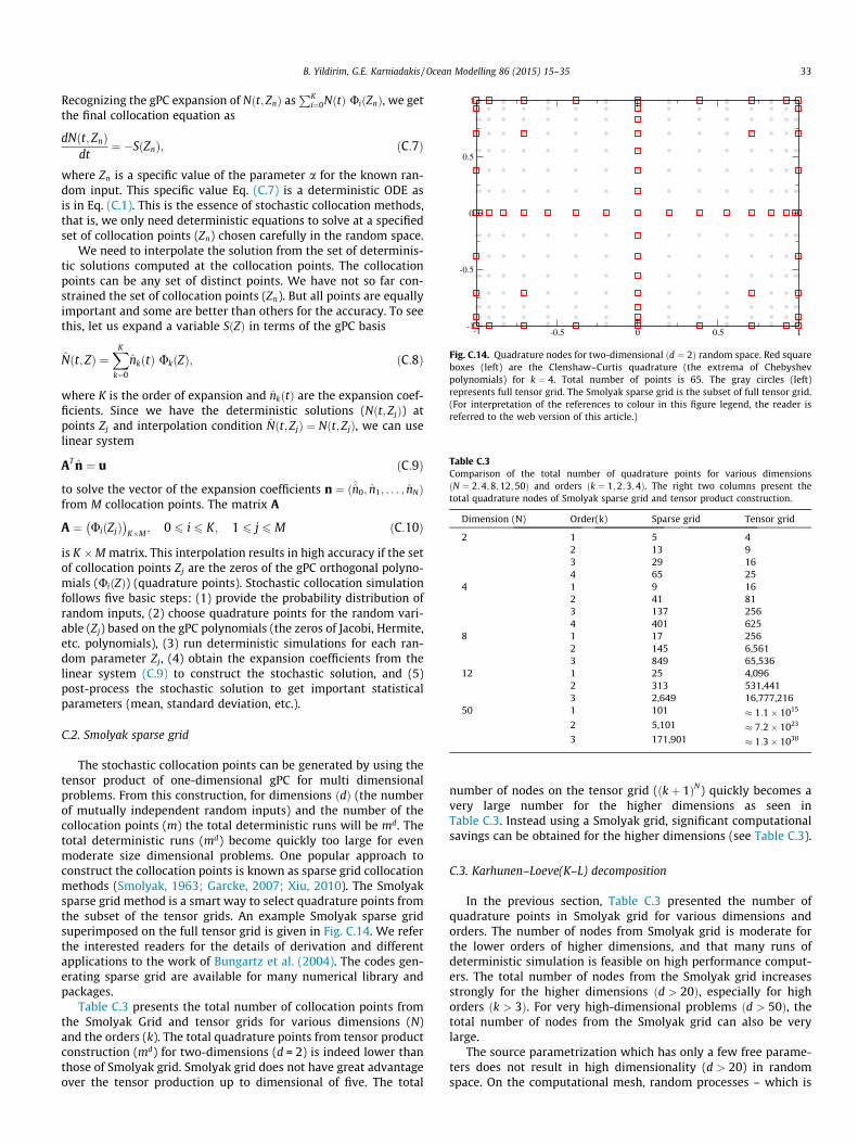
-1 -0.5 0 0.5 1-1

-0.5

0

0.5

1

Fig. C.14. Quadrature nodes for two-dimensional ðd ¼ 2Þ random space. Red squareboxes (left) are the Clenshaw–Curtis quadrature (the extrema of Chebyshevpolynomials) for k ¼ 4. Total number of points is 65. The gray circles (left)represents full tensor grid. The Smolyak sparse grid is the subset of full tensor grid.(For interpretation of the references to colour in this figure legend, the reader isreferred to the web version of this article.)

Table C.3Comparison of the total number of quadrature points for various dimensionsðN ¼ 2;4;8;12;50Þ and orders ðk ¼ 1;2;3;4Þ. The right two columns present thetotal quadrature nodes of Smolyak sparse grid and tensor product construction.

Dimension (N) Order(k) Sparse grid Tensor grid

2 1 5 42 13 93 29 164 65 25

4 1 9 162 41 813 137 2564 401 625

8 1 17 2562 145 6,5613 849 65,536

12 1 25 4,0962 313 531,4413 2,649 16,777,216

50 1 101 1:1� 1015

2 5,101 7:2� 1023

3 171,901 1:3� 1030

B. Yildirim, G.E. Karniadakis / Ocean Modelling 86 (2015) 15–35 33

Recognizing the gPC expansion of Nðt; ZnÞ asPK

i¼0NðtÞ UiðZnÞ, we getthe final collocation equation as

dNðt; ZnÞdt

¼ �SðZnÞ; ðC:7Þ

where Zn is a specific value of the parameter a for the known ran-dom input. This specific value Eq. (C.7) is a deterministic ODE asis in Eq. (C.1). This is the essence of stochastic collocation methods,that is, we only need deterministic equations to solve at a specifiedset of collocation points (Zn) chosen carefully in the random space.

We need to interpolate the solution from the set of determinis-tic solutions computed at the collocation points. The collocationpoints can be any set of distinct points. We have not so far con-strained the set of collocation points (Zn). But all points are equallyimportant and some are better than others for the accuracy. To seethis, let us expand a variable SðZÞ in terms of the gPC basis

N̂ðt; ZÞ ¼XK

k¼0

n̂kðtÞ UkðZÞ; ðC:8Þ

where K is the order of expansion and n̂kðtÞ are the expansion coef-ficients. Since we have the deterministic solutions (Nðt; ZjÞ) atpoints Zj and interpolation condition N̂ðt; ZjÞ ¼ Nðt; ZjÞ, we can uselinear system

AT n̂ ¼ u ðC:9Þ

to solve the vector of the expansion coefficients n ¼ ð^̂n0; n̂1; . . . ; n̂NÞfrom M collocation points. The matrix A

A ¼ UiðZjÞ� �

K�M ; 0 6 i 6 K; 1 6 j 6 M ðC:10Þ

is K �M matrix. This interpolation results in high accuracy if the setof collocation points Zj are the zeros of the gPC orthogonal polyno-mials (UiðZÞ) (quadrature points). Stochastic collocation simulationfollows five basic steps: (1) provide the probability distribution ofrandom inputs, (2) choose quadrature points for the random vari-able (Zj) based on the gPC polynomials (the zeros of Jacobi, Hermite,etc. polynomials), (3) run deterministic simulations for each ran-dom parameter Zj, (4) obtain the expansion coefficients from thelinear system (C.9) to construct the stochastic solution, and (5)post-process the stochastic solution to get important statisticalparameters (mean, standard deviation, etc.).

C.2. Smolyak sparse grid

The stochastic collocation points can be generated by using thetensor product of one-dimensional gPC for multi dimensionalproblems. From this construction, for dimensions ðdÞ (the numberof mutually independent random inputs) and the number of thecollocation points (m) the total deterministic runs will be md. Thetotal deterministic runs (md) become quickly too large for evenmoderate size dimensional problems. One popular approach toconstruct the collocation points is known as sparse grid collocationmethods (Smolyak, 1963; Garcke, 2007; Xiu, 2010). The Smolyaksparse grid method is a smart way to select quadrature points fromthe subset of the tensor grids. An example Smolyak sparse gridsuperimposed on the full tensor grid is given in Fig. C.14. We referthe interested readers for the details of derivation and differentapplications to the work of Bungartz et al. (2004). The codes gen-erating sparse grid are available for many numerical library andpackages.

Table C.3 presents the total number of collocation points fromthe Smolyak Grid and tensor grids for various dimensions (N)and the orders (k). The total quadrature points from tensor productconstruction (md) for two-dimensions (d = 2) is indeed lower thanthose of Smolyak grid. Smolyak grid does not have great advantageover the tensor production up to dimensional of five. The total

number of nodes on the tensor grid (ðkþ 1ÞN) quickly becomes avery large number for the higher dimensions as seen inTable C.3. Instead using a Smolyak grid, significant computationalsavings can be obtained for the higher dimensions (see Table C.3).

C.3. Karhunen–Loeve(K–L) decomposition

In the previous section, Table C.3 presented the number ofquadrature points in Smolyak grid for various dimensions andorders. The number of nodes from Smolyak grid is moderate forthe lower orders of higher dimensions, and that many runs ofdeterministic simulation is feasible on high performance comput-ers. The total number of nodes from the Smolyak grid increasesstrongly for the higher dimensions ðd > 20Þ, especially for highorders ðk > 3Þ. For very high-dimensional problems ðd > 50Þ, thetotal number of nodes from the Smolyak grid can also be verylarge.

The source parametrization which has only a few free parame-ters does not result in high dimensionality (d > 20) in randomspace. On the computational mesh, random processes – which is

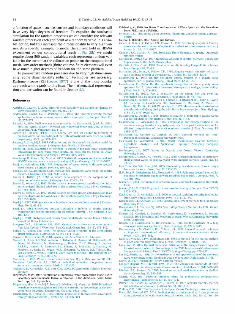
34 B. Yildirim, G.E. Karniadakis / Ocean Modelling 86 (2015) 15–35

a function of space – such as current and boundary conditions willhave very high degrees of freedom. To expedite the stochasticsimulation for the random processes we can consider the relevantrandom process on each grid point as a random variable. It is a via-ble option, but this increases the dimensionality to very high val-ues. As a specific example, to model the current field in HISWAexperiment on our computational mesh in Fig. 2(b) we mightrequire about 500 random variables; each represents random var-iable for the current at the collocation points on the computationalmesh. Low-order methods (finite volume, finite element) will evenhave much higher degrees of freedom for the same problem.

To parametrize random processes due to very high dimension-ality, some dimensionality reduction techniques are necessary.Karhunen–Loeve (KL) (Loeve, 1977) is one of the most popularapproach with regards to this issue. The mathematical representa-tion and derivation can be found in Section 5.3.

References

Abdalla, S., Cavaleri, L., 2002. Effect of wind variability and variable air density onwave modelling. J. Geophys. Res. 107 (C7), 17.

Andreassen, Øyvind, Lie, I., Wasberg, C.E., 1994. The spectral viscosity methodapplied to simulation of waves in a stratified atmosphere. J. Comput. Phys. 110(2), 257–273.

Battjes, J.A., 1994. Shallow water wave modeling. In: Isaacson, M., Quick, M. (Eds.),Proc. Int. Symp.: Waves – Physical and Numerical Modelling, Univ. of BritishColumbia. ASCE, Vancouver, pp. 1–23.

Battjes, J.A., Janssen, J.P.F.M., 1978. Energy loss and set-up due to breaking ofrandom waves. In: Proceedings of the 16th International Conference on CoastalEngineering. ASCE, pp. 569–587.

Battjes, J.A., Stive, M.J.F., 1985. Calibration and verification of a dissipation model forrandom breaking waves. J. Geophys. Res. 90 (C5), 9159–9167.

Benoit, M., 2005. Evaluation of methods to compute the non-linear quadrupletinteractions for deep-water wave spectra. In: Proc. 5th Int. Symp. on OceanWaves, Measurement and Analysis, WAVES 2005. ASCE.

Bonekamp, H., Komen, G.J., Sterl, A., 2002. Statistical comparisons of observed andECMWF modeled open ocean surface drag. J. Phys. Oceanogr. 32, 1010–1027.

Booij, N., Holthuijsen, L.H., 1987. Propagation of ocean waves in discrete spectralwave models. J. Comput. Phys. 68, 307–326.

Booij, N., Ris, R.C., Holthuijsen, L.H., 1999. A third-generation wave model for coastalregions. J. Geophys. Res. 104, 7649–7666.

Bouws, E., Battjes, J.A., 1982. A monte Carlo approach to the computation ofrefraction of water waves. J. Geophys. Res. 87 (C8), 15.

Bouws, E., Komen, G.J., 1983. On the balance between growth and dissipation in anextreme depth-limited wind-sea in the southern North Sea. J. Phys. Oceanogr.13, 1653–1658.

Bouws, E., Komen, G.J., 1983. On the balance between growth and dissipation in anextreme depth-limited wind-sea in the southern North Sea. J. Phys. Oceanogr.13, 1653–1658.

Boyd, J.P., 1987. Orthogonal rational functions on a semi-infinite interval. J. Comput.Phys. 70 (1), 63–88.

Boyd, J.P., 1988. Chebyshev domain truncation is inferior to Fourier domaintruncation for solving problems on an infinite interval. J. Sci. Comput. 3 (2),109–120.

Boyd, J.P., 2001. Chebyshev and Fourier Spectral Methods: Second Revised Edition,second ed. Dover Publications.

Breugem, W.A., Holthuijsen, L.H., 2007. Generalized shallow water wave growthfrom lake George. J. Waterway, Port, Coastal, Ocean Eng. 133 (3), 173–182.

Buizza, R., Palmer, T.N., 1995. The singular-vector structure of the atmosphericglobal circulation. J. Atmos. Sci. 52 (9), 1434–1456.

Bungartz, H.-J., Griebel, M., 2004. Sparse grids. Acta Numer. 13, 147–269.Cavaleri, L., Alves, J.-H.G.M., Ardhuin, F., Babanin, A., Banner, M., Belibassakis, K.,

Benoit, M., Donelan, M., Groeneweg, J., Herbers, T.H.C., Hwang, P., Janssen,P.A.E.M., Janssen, T., Lavrenov, I.V., Magne, R., Monbaliu, J., Onorato, M.,Polnikov, V., Resio, D., Rogers, W.E., Sheremet, A., Smith, J.M., Tolman, H.L.,van Vledder, G., Wolf, J., Young, I., 2007. Wave modelling – the state of the art.Prog. Oceanogr. 75 (4), 603–674.

Charnock, H., 1955. Wind stress on a water surface. Q. J. R. Meteorol. Soc. 81, 639.Clenshaw, C.W., Curtis, A.R., 1960. A method of numerical integration on an

automatic computer. Numer. Math. 2, 197–205.Cockburn, B., Karniadakis, G.E., Shu, C.W., 2000. Discontinuous Galerkin Methods.

Springer.Dingemans, M.W., 1987. Verification of numerical wave propagation models with

laboratory measurements: Hiswa verification in the directional wave basin.Tech. rep., Delft Hydraulics.

Dingemans, M.W., Stive, M.J.F., Bosma, J., deVriend, H.J., Vogel, J.A., 1986. Directionalnearshore wave propagation and induced currents. In: Proceedings of the 20thConference on Coastal Engineering. ASCE, pp. 1092–1106.

Ehrendorfer, M., Tribbia, J.J., 1997. Optimal prediction of forecast error covariancesthrough singular vectors. J. Atmos. Sci. 54, 286–313.

Eldeberky, Y., 1996. Nonlinear Transformation of Wave Spectra in the NearshoreZone (Ph.D. thesis). TUDelft.

Fishman, G.S., 1996. Monte Carlo: Concepts, Algorithms, and Applications. Springer-Verlag.

Garcke, J., TUBerlin, 2007. Sparse grid tutorial.Gelaro, R., Buizza, R., Palmer, T.N., Klinker, E., 1997. Sensitivity analysis of forecast

errors and the construction of optimal perturbations using singular vectors. J.Atmos. Sci. 55, 1012–1037.

Ghanem, R.G., Spanos, P., 1991. Stochastic Finite Elements: A Spectral Approach.Springer-Verlag.

Gottlieb, D., Orszag, S.A., 1977. Numerical Analysis of Spectral Methods: Theory andApplications. SIAM-CMBS, Philadelphia.

Gottlieb, S., Shu, C.-W., 1998. Total variation diminishing Runge–Kutta schemes.Math. Comput 67, 73–85.

Hartmann, D.L., Buizza, R., Palmer, T.N., 1995. Singular vectors: the effect of spatialscale on linear growth of disturbances. J. Atmos. Sci. 52, 3885–3894.

Hasselmann, K., 1962. On the non-linear energy transfer in a gravity wavespectrum, part 1: general theory. J. Fluid Mech. 12, 481–501.

Hasselmann, K., 1963a. On the non-linear energy transfer in a gravity wavespectrum Part 2: conservation theorems; wave-particle analogy; irreversibility.J. Fluid Mech. 15, 273–282.

Hasselmann, K., 1963b. Part 3. evaluation on the energy flux and swell-seainteraction for a Neumann spectrum. J. Fluid Mech. 15, 467–483.

Hasselmann, K., Barnett, T.P., Bouws, E., Carlson, H., Cartwright, D.E., Enke, K., Ewing,J.A., Gienapp, H., Hasselmann, D.E., Kruseman, P., Meerburg, A., Müller, P.,Olbers, D.J., Richter, K., Sell, W., Walden, H., 1973. Measurements of wind-wavegrowth and swell decay during the joint North Sea wave project. Deut. Hydrogr.Z. 8 (12), 1–95, suppl. A..

Hasselmann, K., Collins, J.I., 1968. Spectral dissipation of finite depth gravity wavesdue to turbulent bottom friction. J. Mar. Res. 26, 1–12.

Hasselmann, S., Hasselmann, K., 1985. Computation and parametrization of thenonlinear energy transfer in a gravity-wave spectrum. part I: a new method forefficient computations of the exact nonlinear transfer. J. Phys. Oceanogr. 15,1369–1377.

Hesthaven, J.S., Gottlieb, S., Gottlieb, D., 2007. Spectral Methods for Time-Dependent Problems. Cambridge University Press.

Hesthaven, J.S., Warburton, T., 2007. Nodal Discontinuous Galerkin Methods:Algorithms, Analysis, and Applications. Springer Publishing Company,Incorporated.

Holthuijsen, L.H., 2007. Waves in Oceanic and Coastal Waters. CambridgeUniversity Press.

Holthuijsen, L.H., Booij, N., Herbers, T.H.C., 1989. A prediction model for stationary,short-crested waves in shallow water with ambient currents. Coast. Eng. 13,23–54.

Hsu, T.-W., Ou, S.-H., Liau, J.-M., 2005. Hindcasting nearshore wind waves using afem code for swan. Coast. Eng. 52, 177–195.

If, F., Berg, P., Christiansen, P.L., Skovgaard, O., 1987. Split-step spectral method fornonlinear Schrödinger equation with absorbing boundaries. J. Comput. Phys. 72(2), 501–503.

Janssen, P., 2004. The Interaction of Ocean Waves and Wind. Cambridge UniversityPress.

Janssen, P.A.E.M., 2008. Progress in ocean wave forecasting. J. Comput. Phys. 227 (7),3572–3594.

Karamanos, G.-S., Karniadakis, G.E., 2000. A spectral vanishing viscosity method forlarge-eddy simulations. J. Comput. Phys. 163 (1), 22–50.

Karniadakis, G.E., Sherwin, S.J., 1999. Spectral/hp Element Methods for CFD. OxfordUniversity Press.

Karniadakis, G.E., Sherwin, S.J., 2005. Spectral/hp Element Methods for CFD,, OxfordUniversity Press.

Komen, G.J., Cavaleri, L., Donelan, M., Hasselmann, K., Hasselmann, S., Janssen,P.A.E.M., 1994. Dynamics and Modeling of Ocean Waves. Cambridge UniversityPress, Cambridge.

Komen, G.J., Hasselmann, K., Hasselmann, S., 1984. On the existence of a fullydeveloped wind sea spectrum. J. Phys. Oceanogr. 14, 1271–1285.

Krasnopolsky, V.M., Chalikov, D.V., Tolman, H.L., 2002. A neural network techniqueto improve computational efficiency of numerical oceanic models. OceanModel. 4 (34), 363–383.

Kuik, A.J., Vledder, G.P.V., Holthuijsen, L.H., 1988. A Method for the routine analysisof pitch-and-roll buoy wave data. J. Phys. Oceanogr. 18, 1020–1034.

Lavrenov, I.V., 2003. Optimal numerical realization of the energy balance equationfor wind wave models. In: Proceedings of the 2003 International Conference onComputational Science: Part II. ICCS’03. Springer-Verlag, pp. 179–187.

Lin, R.Q., Perrie, W., 1998. On the mathematics and approximation of the nonlinearwave-wave interactions. Nonlinear Ocean Waves, Adv. Fluid Mech., 61–88.

Loeve, M., 1977. Probability Theory. Springer-Verlag.Longuet-Higgins, M.S., Stewart, R.W., 1961. The changes in amplitude of short

gravity waves on steady non-uniform currents. J. Fluid Mech. 10 (04), 529–549.Madsen, P.A., Srenson, O., 1993. Bound waves and triad interactions in shallow

water. Ocean Eng. 20, 359–388.Morris, M.D., 1991. Factorial sampling plans for preliminary computational

experiments. Technometrics 33 (2), 161–174.Palmer, T.N., Gelaro, R., Barkmeijer, J., Buizza, R., 1997. Singular Vectors, metrics,

and adaptive observations. J. Atmos. Sci. 54, 286–313.Phillips, O.M., 1966. The Dynamics of the Upper Ocean. Cambridge University Press.Plant, N.G., Holland, K.T., 2011. Prediction and assimilation of surf-zone processes

using a Bayesian network: Part I: forward models. Coast. Eng. 58 (1), 119–130.

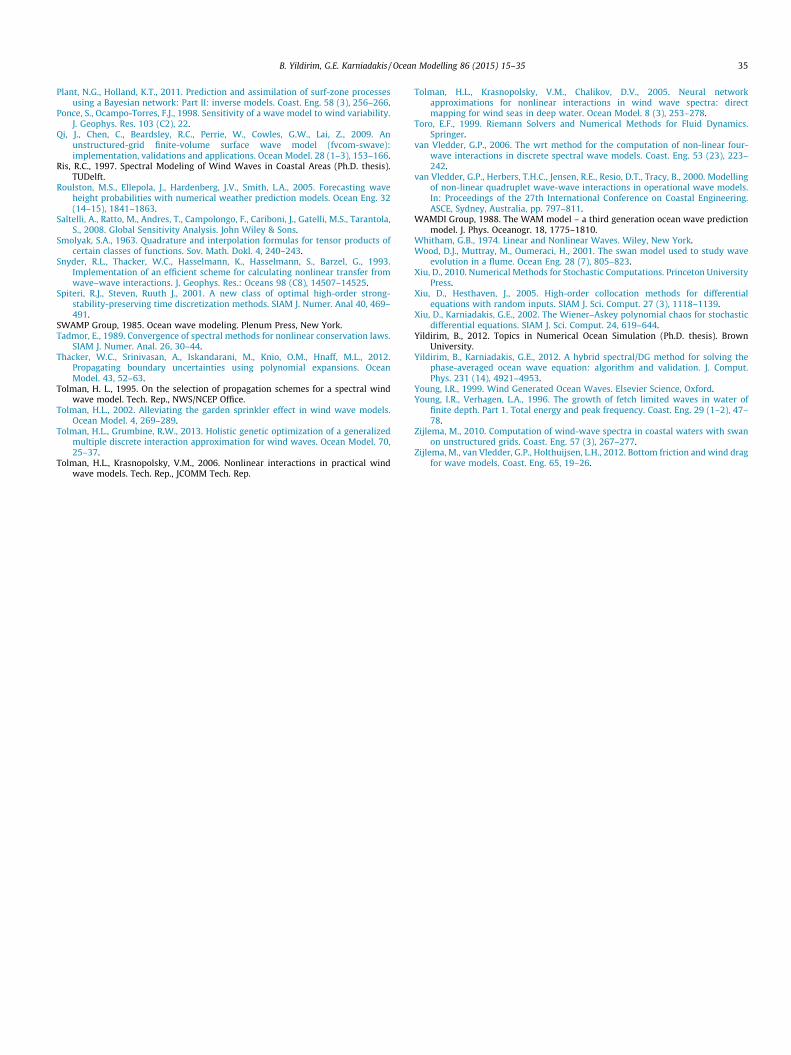
B. Yildirim, G.E. Karniadakis / Ocean Modelling 86 (2015) 15–35 35

Plant, N.G., Holland, K.T., 2011. Prediction and assimilation of surf-zone processesusing a Bayesian network: Part II: inverse models. Coast. Eng. 58 (3), 256–266.

Ponce, S., Ocampo-Torres, F.J., 1998. Sensitivity of a wave model to wind variability.J. Geophys. Res. 103 (C2), 22.

Qi, J., Chen, C., Beardsley, R.C., Perrie, W., Cowles, G.W., Lai, Z., 2009. Anunstructured-grid finite-volume surface wave model (fvcom-swave):implementation, validations and applications. Ocean Model. 28 (1–3), 153–166.

Ris, R.C., 1997. Spectral Modeling of Wind Waves in Coastal Areas (Ph.D. thesis).TUDelft.

Roulston, M.S., Ellepola, J., Hardenberg, J.V., Smith, L.A., 2005. Forecasting waveheight probabilities with numerical weather prediction models. Ocean Eng. 32(14–15), 1841–1863.

Saltelli, A., Ratto, M., Andres, T., Campolongo, F., Cariboni, J., Gatelli, M.S., Tarantola,S., 2008. Global Sensitivity Analysis. John Wiley & Sons.

Smolyak, S.A., 1963. Quadrature and interpolation formulas for tensor products ofcertain classes of functions. Sov. Math. Dokl. 4, 240–243.

Snyder, R.L., Thacker, W.C., Hasselmann, K., Hasselmann, S., Barzel, G., 1993.Implementation of an efficient scheme for calculating nonlinear transfer fromwave–wave interactions. J. Geophys. Res.: Oceans 98 (C8), 14507–14525.

Spiteri, R.J., Steven, Ruuth J., 2001. A new class of optimal high-order strong-stability-preserving time discretization methods. SIAM J. Numer. Anal 40, 469–491.

SWAMP Group, 1985. Ocean wave modeling. Plenum Press, New York.Tadmor, E., 1989. Convergence of spectral methods for nonlinear conservation laws.

SIAM J. Numer. Anal. 26, 30–44.Thacker, W.C., Srinivasan, A., Iskandarani, M., Knio, O.M., Hnaff, M.L., 2012.

Propagating boundary uncertainties using polynomial expansions. OceanModel. 43, 52–63.

Tolman, H. L., 1995. On the selection of propagation schemes for a spectral windwave model. Tech. Rep., NWS/NCEP Office.

Tolman, H.L., 2002. Alleviating the garden sprinkler effect in wind wave models.Ocean Model. 4, 269–289.

Tolman, H.L., Grumbine, R.W., 2013. Holistic genetic optimization of a generalizedmultiple discrete interaction approximation for wind waves. Ocean Model. 70,25–37.

Tolman, H.L., Krasnopolsky, V.M., 2006. Nonlinear interactions in practical windwave models. Tech. Rep., JCOMM Tech. Rep.

Tolman, H.L., Krasnopolsky, V.M., Chalikov, D.V., 2005. Neural networkapproximations for nonlinear interactions in wind wave spectra: directmapping for wind seas in deep water. Ocean Model. 8 (3), 253–278.

Toro, E.F., 1999. Riemann Solvers and Numerical Methods for Fluid Dynamics.Springer.

van Vledder, G.P., 2006. The wrt method for the computation of non-linear four-wave interactions in discrete spectral wave models. Coast. Eng. 53 (23), 223–242.

van Vledder, G.P., Herbers, T.H.C., Jensen, R.E., Resio, D.T., Tracy, B., 2000. Modellingof non-linear quadruplet wave-wave interactions in operational wave models.In: Proceedings of the 27th International Conference on Coastal Engineering.ASCE, Sydney, Australia, pp. 797–811.

WAMDI Group, 1988. The WAM model – a third generation ocean wave predictionmodel. J. Phys. Oceanogr. 18, 1775–1810.

Whitham, G.B., 1974. Linear and Nonlinear Waves. Wiley, New York.Wood, D.J., Muttray, M., Oumeraci, H., 2001. The swan model used to study wave

evolution in a flume. Ocean Eng. 28 (7), 805–823.Xiu, D., 2010. Numerical Methods for Stochastic Computations. Princeton University

Press.Xiu, D., Hesthaven, J., 2005. High-order collocation methods for differential

equations with random inputs. SIAM J. Sci. Comput. 27 (3), 1118–1139.Xiu, D., Karniadakis, G.E., 2002. The Wiener–Askey polynomial chaos for stochastic

differential equations. SIAM J. Sci. Comput. 24, 619–644.Yildirim, B., 2012. Topics in Numerical Ocean Simulation (Ph.D. thesis). Brown

University.Yildirim, B., Karniadakis, G.E., 2012. A hybrid spectral/DG method for solving the

phase-averaged ocean wave equation: algorithm and validation. J. Comput.Phys. 231 (14), 4921–4953.

Young, I.R., 1999. Wind Generated Ocean Waves. Elsevier Science, Oxford.Young, I.R., Verhagen, L.A., 1996. The growth of fetch limited waves in water of

finite depth. Part 1. Total energy and peak frequency. Coast. Eng. 29 (1–2), 47–78.

Zijlema, M., 2010. Computation of wind-wave spectra in coastal waters with swanon unstructured grids. Coast. Eng. 57 (3), 267–277.

Zijlema, M., van Vledder, G.P., Holthuijsen, L.H., 2012. Bottom friction and wind dragfor wave models. Coast. Eng. 65, 19–26.