Embed Size (px)
Citation preview
Computation
Visualization
Programming
MATLAB Function ReferenceVolume 3: P - ZVersion 6
MATLAB®
The Language of Technical Computing
How to Contact The MathWorks:
508-647-7000 Phone
508-647-7001 Fax
The MathWorks, Inc. Mail3 Apple Hill DriveNatick, MA 01760-2098
http://www.mathworks.com Webftp.mathworks.com Anonymous FTP servercomp.soft-sys.matlab Newsgroup
[email protected] Technical [email protected] Product enhancement [email protected] Bug [email protected] Documentation error [email protected] Subscribing user [email protected] Order status, license renewals, [email protected] Sales, pricing, and general information
MATLAB Function Reference Volume 3: P- Z COPYRIGHT 1984 - 2000 by The MathWorks, Inc.The software described in this document is furnished under a license agreement. The software may be usedor copied only under the terms of the license agreement. No part of this manual may be photocopied or repro-duced in any form without prior written consent from The MathWorks, Inc.
FEDERAL ACQUISITION: This provision applies to all acquisitions of the Program and Documentation byor for the federal government of the United States. By accepting delivery of the Program, the governmenthereby agrees that this software qualifies as "commercial" computer software within the meaning of FARPart 12.212, DFARS Part 227.7202-1, DFARS Part 227.7202-3, DFARS Part 252.227-7013, and DFARS Part252.227-7014. The terms and conditions of The MathWorks, Inc. Software License Agreement shall pertainto the government’s use and disclosure of the Program and Documentation, and shall supersede anyconflicting contractual terms or conditions. If this license fails to meet the government’s minimum needs oris inconsistent in any respect with federal procurement law, the government agrees to return the Programand Documentation, unused, to MathWorks.
MATLAB, Simulink, Stateflow, Handle Graphics, and Real-Time Workshop are registered trademarks, andTarget Language Compiler is a trademark of The MathWorks, Inc.
Other product or brand names are trademarks or registered trademarks of their respective holders.
Printing History: December 1996 First printing New for MATLAB 5.0 (Release 10)June 1997 Revised for 5.1 Online version, MATLAB 5.1October 1997 Revised for 5.2 Online version, MATLAB 5.2January 1999 Revised for 5.3 Online version (Release 11)June 1999 Second printing MATLAB 5.3 (Release 11)November 2000 Revised for 6.0 Online version (Release 12)
iii
Contents
1Functions by Category
General Purpose Commands . . . . . . . . . . . . . . . . . . . . . . . . . . . vii
Operators and Special Characters . . . . . . . . . . . . . . . . . . . . . . . ix
Logical Functions . . . . . . . . . . . . . . . . . . . . . . . . . . . . . . . . . . . . . . . x
Language Constructs and Debugging . . . . . . . . . . . . . . . . . . . . . x
Elementary Matrices and Matrix Manipulation . . . . . . . . . . xii
Specialized Matrices . . . . . . . . . . . . . . . . . . . . . . . . . . . . . . . . . . xiv
Elementary Math Functions . . . . . . . . . . . . . . . . . . . . . . . . . . . xiv
Specialized Math Functions . . . . . . . . . . . . . . . . . . . . . . . . . . . . xv
Coordinate System Conversion . . . . . . . . . . . . . . . . . . . . . . . . xvi
Matrix Functions - Numerical Linear Algebra . . . . . . . . . . . xvi
Data Analysis and Fourier Transform Functions . . . . . . . xvii
Polynomial and Interpolation Functions . . . . . . . . . . . . . . . xviii
Function Functions – Nonlinear Numerical Methods . . . . . xix
Sparse Matrix Functions . . . . . . . . . . . . . . . . . . . . . . . . . . . . . . . xx
Sound Processing Functions . . . . . . . . . . . . . . . . . . . . . . . . . . xxii
Character String Functions . . . . . . . . . . . . . . . . . . . . . . . . . . . xxii
File I/O Functions . . . . . . . . . . . . . . . . . . . . . . . . . . . . . . . . . . . . xxiv
iv Contents
Bitwise Functions . . . . . . . . . . . . . . . . . . . . . . . . . . . . . . . . . . . . xxv
Structure Functions . . . . . . . . . . . . . . . . . . . . . . . . . . . . . . . . . . xxv
MATLAB Object Functions . . . . . . . . . . . . . . . . . . . . . . . . . . . . xxv
MATLAB Interface to Java . . . . . . . . . . . . . . . . . . . . . . . . . . . . xxv
Cell Array Functions . . . . . . . . . . . . . . . . . . . . . . . . . . . . . . . . . xxvi
Multidimensional Array Functions . . . . . . . . . . . . . . . . . . . . xxvi
Plotting and Data Visualization . . . . . . . . . . . . . . . . . . . . . . . xxvi
Graphical User Interfaces . . . . . . . . . . . . . . . . . . . . . . . . . . xxxiii
Serial Port I/O . . . . . . . . . . . . . . . . . . . . . . . . . . . . . . . . . . . . . . xxxiv
Volume 3 Reference
Index
1Functions by Category
1-vi
This section lists MATLAB functions grouped by functional area.
General Purpose Commands
Operators and Special Characters
Logical Functions
Language Constructs and Debugging
Elementary Matrices and Matrix Manipulation
Specialized Matrices
Elementary Math Functions
Specialized Math Functions
Coordinate System Conversion
Matrix Functions - Numerical Linear Algebra
Data Analysis and Fourier Transform Functions
Polynomial and Interpolation Functions
Function Functions – Nonlinear Numerical Methods
Sparse Matrix Functions
Sound Processing Functions
Character String Functions
File I/O Functions
Bitwise Functions
Structure Functions
MATLAB Object Functions
MATLAB Interface to Java
Cell Array Functions
1-vii
General Purpose Commands
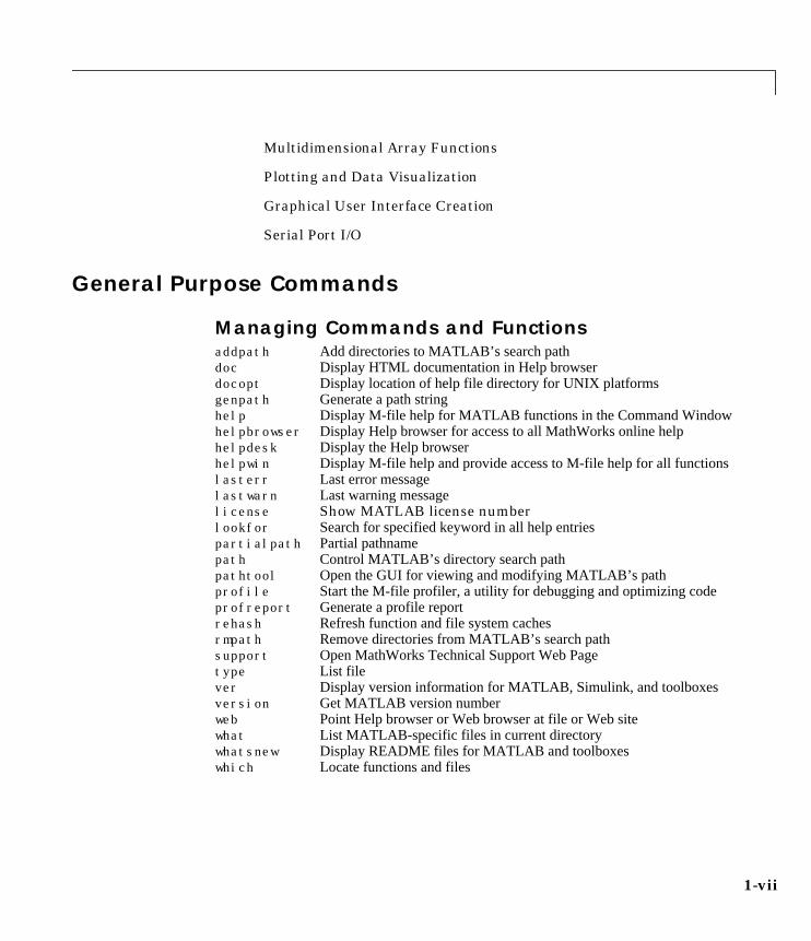
Managing Commands and Functionsaddpath Add directories to MATLAB’s search pathdoc Display HTML documentation in Help browserdocopt Display location of help file directory for UNIX platformsgenpath Generate a path stringhelp Display M-file help for MATLAB functions in the Command Windowhelpbrowser Display Help browser for access to all MathWorks online helphelpdesk Display the Help browserhelpwin Display M-file help and provide access to M-file help for all functionslasterr Last error messagelastwarn Last warning messagelicense Show MATLAB license numberlookfor Search for specified keyword in all help entriespartialpath Partial pathnamepath Control MATLAB’s directory search pathpathtool Open the GUI for viewing and modifying MATLAB’s pathprofile Start the M-file profiler, a utility for debugging and optimizing codeprofreport Generate a profile reportrehash Refresh function and file system cachesrmpath Remove directories from MATLAB’s search pathsupport Open MathWorks Technical Support Web Pagetype List filever Display version information for MATLAB, Simulink, and toolboxesversion Get MATLAB version numberweb Point Help browser or Web browser at file or Web sitewhat List MATLAB-specific files in current directorywhatsnew Display README files for MATLAB and toolboxeswhich Locate functions and files
Multidimensional Array Functions
Plotting and Data Visualization
Graphical User Interface Creation
Serial Port I/O
1-viii
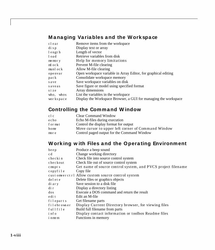
Managing Variables and the Workspaceclear Remove items from the workspacedisp Display text or arraylength Length of vectorload Retrieve variables from diskmemory Help for memory limitationsmlock Prevent M-file clearingmunlock Allow M-file clearingopenvar Open workspace variable in Array Editor, for graphical editingpack Consolidate workspace memorysave Save workspace variables on disksaveas Save figure or model using specified formatsize Array dimensionswho, whos List the variables in the workspaceworkspace Display the Workspace Browser, a GUI for managing the workspace
Controlling the Command Windowclc Clear Command Windowecho Echo M-files during executionformat Control the display format for outputhome Move cursor to upper left corner of Command Windowmore Control paged output for the Command Window
Working with Files and the Operating Environmentbeep Produce a beep soundcd Change working directorycheckin Check file into source control systemcheckout Check file out of source control systemcmopts Get name of source control system, and PVCS project filenamecopyfile Copy filecustomverctrlAllow custom source control systemdelete Delete files or graphics objectsdiary Save session to a disk filedir Display a directory listingdos Execute a DOS command and return the resultedit Edit an M-filefileparts Get filename partsfilebrowser Display Current Directory browser, for viewing filesfullfile Build full filename from partsinfo Display contact information or toolbox Readme filesinmem Functions in memory
1-ix
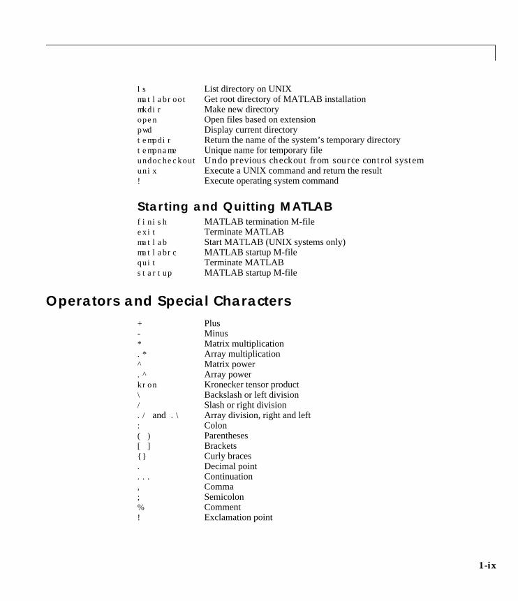
ls List directory on UNIXmatlabroot Get root directory of MATLAB installationmkdir Make new directoryopen Open files based on extensionpwd Display current directorytempdir Return the name of the system’s temporary directorytempname Unique name for temporary fileundocheckout Undo previous checkout from source control systemunix Execute a UNIX command and return the result! Execute operating system command
Starting and Quitting MATLABfinish MATLAB termination M-fileexit Terminate MATLABmatlab Start MATLAB (UNIX systems only)matlabrc MATLAB startup M-filequit Terminate MATLABstartup MATLAB startup M-file
Operators and Special Characters+ Plus- Minus* Matrix multiplication.* Array multiplication^ Matrix power.^ Array powerkron Kronecker tensor product\ Backslash or left division/ Slash or right division./ and .\ Array division, right and left: Colon( ) Parentheses[ ] Brackets Curly braces. Decimal point... Continuation, Comma; Semicolon% Comment! Exclamation point
1-x
' Transpose and quote.' Nonconjugated transpose= Assignment== Equality< > Relational operators& Logical AND| Logical OR~ Logical NOTxor Logical EXCLUSIVE OR
Logical Functionsall Test to determine if all elements are nonzeroany Test for any nonzerosexist Check if a variable or file existsfind Find indices and values of nonzero elementsis* Detect stateisa Detect an object of a given classiskeyword Testif string is a MATLAB keywordisvarname Test if string is a valid variable namelogical Convert numeric values to logicalmislocked True if M-file cannot be cleared
Language Constructs and Debugging
MATLAB as a Programming Languagebuiltin Execute builtin function from overloaded methodeval Interpret strings containing MATLAB expressionsevalc Evaluate MATLAB expression with captureevalin Evaluate expression in workspacefeval Function evaluationfunction Function M-filesglobal Define global variablesnargchk Check number of input argumentspersistent Define persistent variablescript Script M-files
Control Flowbreak Terminate execution offor loop orwhile loop
1-xi
case Case switchcatch Begin catch blockcontinue Pass control to the next iteration offor or while loopelse Conditionally execute statementselseif Conditionally execute statementsend Terminatefor, while, switch, try, andif statements or indicate last
indexerror Display error messagesfor Repeat statements a specific number of timesif Conditionally execute statementsotherwise Default part ofswitch statementreturn Return to the invoking functionswitch Switch among several cases based on expressiontry Begintry blockwarning Display warning messagewhile Repeat statements an indefinite number of times
Interactive Inputinput Request user inputkeyboard Invoke the keyboard in an M-filemenu Generate a menu of choices for user inputpause Halt execution temporarily
Object-Oriented Programmingclass Create object or return class of objectdouble Convert to double precisioninferiorto Inferior class relationshipinline Construct an inline objectint8, int16, int32
Convert to signed integerisa Detect an object of a given classloadobj Extends theload function for user objectssaveobj Save filter for objectssingle Convert to single precisionsuperiorto Superior class relationshipuint8, uint16, uint32
Convert to unsigned integer
Debuggingdbclear Clear breakpoints
1-xii
dbcont Resume executiondbdown Change local workspace contextdbmex Enable MEX-file debuggingdbquit Quit debug modedbstack Display function call stackdbstatus List all breakpointsdbstep Execute one or more lines from a breakpointdbstop Set breakpoints in an M-file functiondbtype List M-file with line numbersdbup Change local workspace context
Function Handlesfunction_handle
MATLAB data type that is a handle to a functionfunctions Return information about a function handlefunc2str Constructs a function name string from a function handlestr2func Constructs a function handle from a function name string
Elementary Matrices and Matrix Manipulation
Elementary Matrices and Arraysblkdiag Construct a block diagonal matrix from input argumentseye Identity matrixlinspace Generate linearly spaced vectorslogspace Generate logarithmically spaced vectorsnumel Number of elements in a matrix or cell arrayones Create an array of all onesrand Uniformly distributed random numbers and arraysrandn Normally distributed random numbers and arrayszeros Create an array of all zeros: (colon) Regularly spaced vector
Special Variables and Constantsans The most recent answercomputer Identify the computer on which MATLAB is runningeps Floating-point relative accuracyi Imaginary unitInf Infinityinputname Input argument name
1-xiii
j Imaginary unitNaN Not-a-Numbernargin, nargout
Number of function argumentsnargoutchk Validate number of output argumentspi Ratio of a circle’s circumference to its diameter,πrealmax Largest positive floating-point numberrealmin Smallest positive floating-point numbervarargin, varargout
Pass or return variable numbers of arguments
Time and Datescalendar Calendarclock Current time as a date vectorcputime Elapsed CPU timedate Current date stringdatenum Serial date numberdatestr Date string formatdatevec Date componentseomday End of monthetime Elapsed timenow Current date and timetic, toc Stopwatch timerweekday Day of the week
Matrix Manipulationcat Concatenate arraysdiag Diagonal matrices and diagonals of a matrixfliplr Flip matrices left-rightflipud Flip matrices up-downrepmat Replicate and tile an arrayreshape Reshape arrayrot90 Rotate matrix 90 degreestril Lower triangular part of a matrixtriu Upper triangular part of a matrix: (colon) Index into array, rearrange array
Vector Functionscross Vector cross productdot Vector dot product
1-xiv
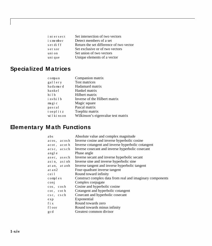
intersect Set intersection of two vectorsismember Detect members of a setsetdiff Return the set difference of two vectorsetxor Set exclusive or of two vectorsunion Set union of two vectorsunique Unique elements of a vector
Specialized Matricescompan Companion matrixgallery Test matriceshadamard Hadamard matrixhankel Hankel matrixhilb Hilbert matrixinvhilb Inverse of the Hilbert matrixmagic Magic squarepascal Pascal matrixtoeplitz Toeplitz matrixwilkinson Wilkinson’s eigenvalue test matrix
Elementary Math Functionsabs Absolute value and complex magnitudeacos, acosh Inverse cosine and inverse hyperbolic cosineacot, acoth Inverse cotangent and inverse hyperbolic cotangentacsc, acsch Inverse cosecant and inverse hyperbolic cosecantangle Phase angleasec, asech Inverse secant and inverse hyperbolic secantasin, asinh Inverse sine and inverse hyperbolic sineatan, atanh Inverse tangent and inverse hyperbolic tangentatan2 Four-quadrant inverse tangentceil Round toward infinitycomplex Construct complex data from real and imaginary componentsconj Complex conjugatecos, cosh Cosine and hyperbolic cosinecot, coth Cotangent and hyperbolic cotangentcsc, csch Cosecant and hyperbolic cosecantexp Exponentialfix Round towards zerofloor Round towards minus infinitygcd Greatest common divisor
1-xv
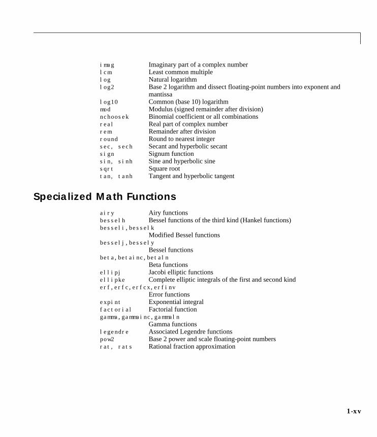
imag Imaginary part of a complex numberlcm Least common multiplelog Natural logarithmlog2 Base 2 logarithm and dissect floating-point numbers into exponent and
mantissalog10 Common (base 10) logarithmmod Modulus (signed remainder after division)nchoosek Binomial coefficient or all combinationsreal Real part of complex numberrem Remainder after divisionround Round to nearest integersec, sech Secant and hyperbolic secantsign Signum functionsin, sinh Sine and hyperbolic sinesqrt Square roottan, tanh Tangent and hyperbolic tangent
Specialized Math Functionsairy Airy functionsbesselh Bessel functions of the third kind (Hankel functions)besseli, besselk
Modified Bessel functionsbesselj, bessely
Bessel functionsbeta, betainc, betaln
Beta functionsellipj Jacobi elliptic functionsellipke Complete elliptic integrals of the first and second kinderf, erfc, erfcx, erfinv
Error functionsexpint Exponential integralfactorial Factorial functiongamma, gammainc, gammaln
Gamma functionslegendre Associated Legendre functionspow2 Base 2 power and scale floating-point numbersrat, rats Rational fraction approximation
1-xvi
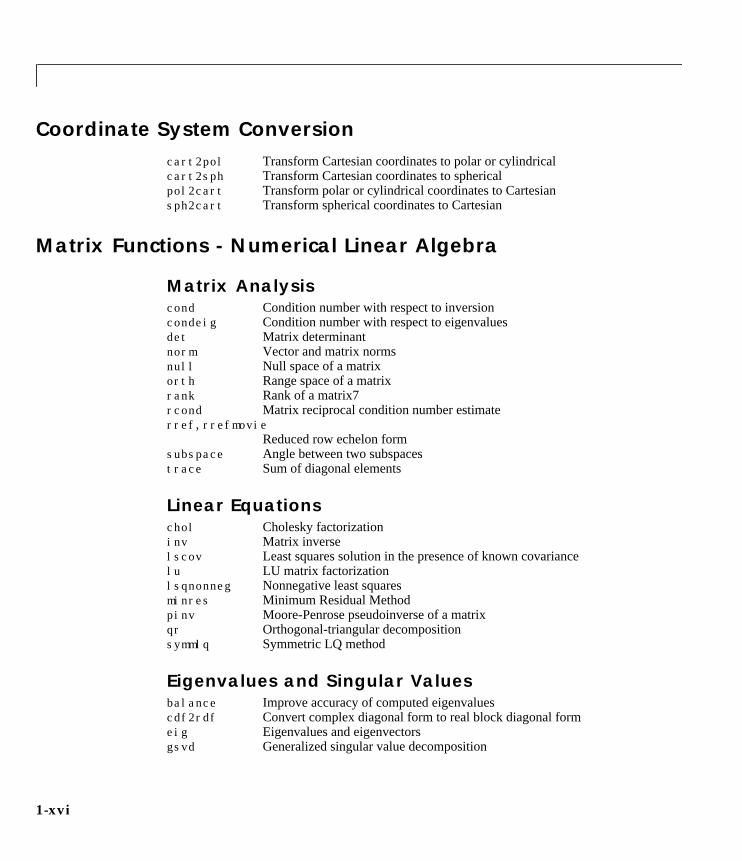
Coordinate System Conversioncart2pol Transform Cartesian coordinates to polar or cylindricalcart2sph Transform Cartesian coordinates to sphericalpol2cart Transform polar or cylindrical coordinates to Cartesiansph2cart Transform spherical coordinates to Cartesian
Matrix Functions - Numerical Linear Algebra
Matrix Analysiscond Condition number with respect to inversioncondeig Condition number with respect to eigenvaluesdet Matrix determinantnorm Vector and matrix normsnull Null space of a matrixorth Range space of a matrixrank Rank of a matrix7rcond Matrix reciprocal condition number estimaterref, rrefmovie
Reduced row echelon formsubspace Angle between two subspacestrace Sum of diagonal elements
Linear Equationschol Cholesky factorizationinv Matrix inverselscov Least squares solution in the presence of known covariancelu LU matrix factorizationlsqnonneg Nonnegative least squaresminres Minimum Residual Methodpinv Moore-Penrose pseudoinverse of a matrixqr Orthogonal-triangular decompositionsymmlq Symmetric LQ method
Eigenvalues and Singular Valuesbalance Improve accuracy of computed eigenvaluescdf2rdf Convert complex diagonal form to real block diagonal formeig Eigenvalues and eigenvectorsgsvd Generalized singular value decomposition
1-xvii
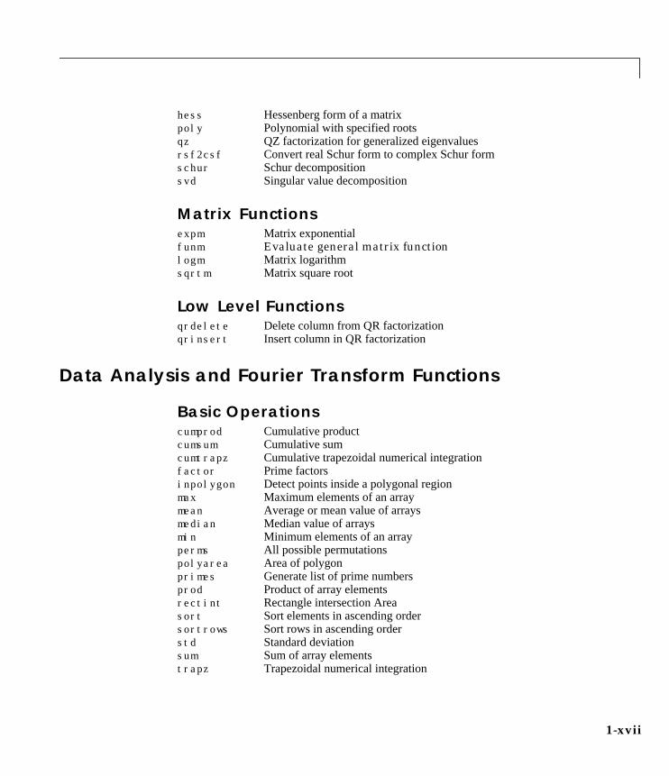
hess Hessenberg form of a matrixpoly Polynomial with specified rootsqz QZ factorization for generalized eigenvaluesrsf2csf Convert real Schur form to complex Schur formschur Schur decompositionsvd Singular value decomposition
Matrix Functionsexpm Matrix exponentialfunm Evaluate general matrix functionlogm Matrix logarithmsqrtm Matrix square root
Low Level Functionsqrdelete Delete column from QR factorizationqrinsert Insert column in QR factorization
Data Analysis and Fourier Transform Functions
Basic Operationscumprod Cumulative productcumsum Cumulative sumcumtrapz Cumulative trapezoidal numerical integrationfactor Prime factorsinpolygon Detect points inside a polygonal regionmax Maximum elements of an arraymean Average or mean value of arraysmedian Median value of arraysmin Minimum elements of an arrayperms All possible permutationspolyarea Area of polygonprimes Generate list of prime numbersprod Product of array elementsrectint Rectangle intersection Areasort Sort elements in ascending ordersortrows Sort rows in ascending orderstd Standard deviationsum Sum of array elementstrapz Trapezoidal numerical integration
1-xviii
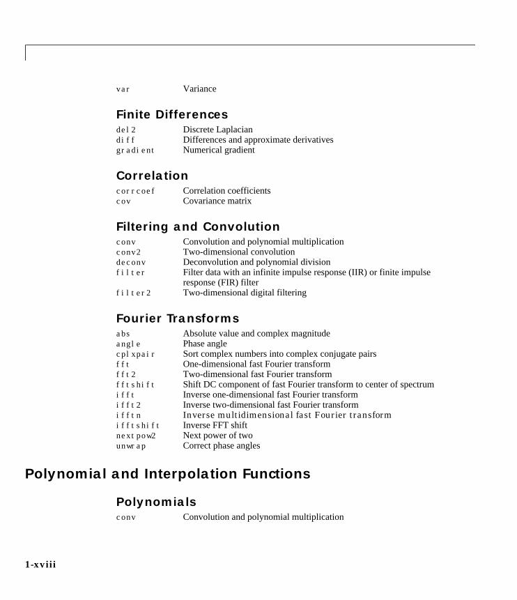
var Variance
Finite Differencesdel2 Discrete Laplaciandiff Differences and approximate derivativesgradient Numerical gradient
Correlationcorrcoef Correlation coefficientscov Covariance matrix
Filtering and Convolutionconv Convolution and polynomial multiplicationconv2 Two-dimensional convolutiondeconv Deconvolution and polynomial divisionfilter Filter data with an infinite impulse response (IIR) or finite impulse
response (FIR) filterfilter2 Two-dimensional digital filtering
Fourier Transformsabs Absolute value and complex magnitudeangle Phase anglecplxpair Sort complex numbers into complex conjugate pairsfft One-dimensional fast Fourier transformfft2 Two-dimensional fast Fourier transformfftshift Shift DC component of fast Fourier transform to center of spectrumifft Inverse one-dimensional fast Fourier transformifft2 Inverse two-dimensional fast Fourier transformifftn Inverse multidimensional fast Fourier transformifftshift Inverse FFT shiftnextpow2 Next power of twounwrap Correct phase angles
Polynomial and Interpolation Functions
Polynomialsconv Convolution and polynomial multiplication
1-xix
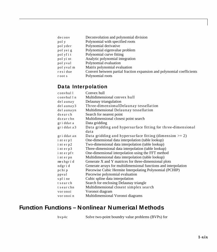
deconv Deconvolution and polynomial divisionpoly Polynomial with specified rootspolyder Polynomial derivativepolyeig Polynomial eigenvalue problempolyfit Polynomial curve fittingpolyint Analytic polynomial integrationpolyval Polynomial evaluationpolyvalm Matrix polynomial evaluationresidue Convert between partial fraction expansion and polynomial coefficientsroots Polynomial roots
Data Interpolationconvhull Convex hullconvhulln Multidimensional convex hulldelaunay Delaunay triangulationdelaunay3 Three-dimensionalDelaunay tessellationdelaunayn Multidimensional Delaunay tessellationdsearch Search for nearest pointdsearchn Multidimensional closest point searchgriddata Data griddinggriddata3 Data gridding and hypersurface fitting for three-dimensional
datagriddatan Data gridding and hypersurface fitting (dimension >= 2)interp1 One-dimensional data interpolation (table lookup)interp2 Two-dimensional data interpolation (table lookup)interp3 Three-dimensional data interpolation (table lookup)interpft One-dimensional interpolation using the FFT methodinterpn Multidimensional data interpolation (table lookup)meshgrid Generate X and Y matrices for three-dimensional plotsndgrid Generate arrays for multidimensional functions and interpolationpchip Piecewise Cubic Hermite Interpolating Polynomial (PCHIP)ppval Piecewise polynomial evaluationspline Cubic spline data interpolationtsearch Search for enclosing Delaunay triangletsearchn Multidimensional closest simplex searchvoronoi Voronoi diagramvoronoin Multidimensional Voronoi diagrams
Function Functions – Nonlinear Numerical Methodsbvp4c Solve two-point boundry value problems (BVPs) for
1-xx
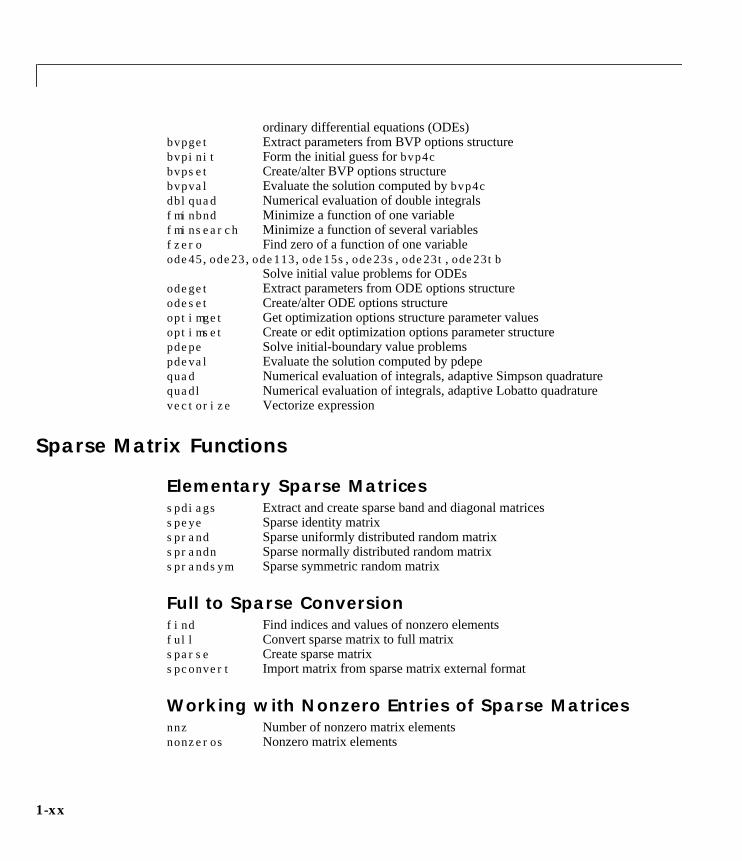
ordinary differential equations (ODEs)bvpget Extract parameters from BVP options structurebvpinit Form the initial guess forbvp4cbvpset Create/alter BVP options structurebvpval Evaluate the solution computed bybvp4cdblquad Numerical evaluation of double integralsfminbnd Minimize a function of one variablefminsearch Minimize a function of several variablesfzero Find zero of a function of one variableode45, ode23, ode113, ode15s, ode23s, ode23t, ode23tb
Solve initial value problems for ODEsodeget Extract parameters from ODE options structureodeset Create/alter ODE options structureoptimget Get optimization options structure parameter valuesoptimset Create or edit optimization options parameter structurepdepe Solve initial-boundary value problemspdeval Evaluate the solution computed by pdepequad Numerical evaluation of integrals, adaptive Simpson quadraturequadl Numerical evaluation of integrals, adaptive Lobatto quadraturevectorize Vectorize expression
Sparse Matrix Functions
Elementary Sparse Matricesspdiags Extract and create sparse band and diagonal matricesspeye Sparse identity matrixsprand Sparse uniformly distributed random matrixsprandn Sparse normally distributed random matrixsprandsym Sparse symmetric random matrix
Full to Sparse Conversionfind Find indices and values of nonzero elementsfull Convert sparse matrix to full matrixsparse Create sparse matrixspconvert Import matrix from sparse matrix external format
Working with Nonzero Entries of Sparse Matricesnnz Number of nonzero matrix elementsnonzeros Nonzero matrix elements
1-xxi
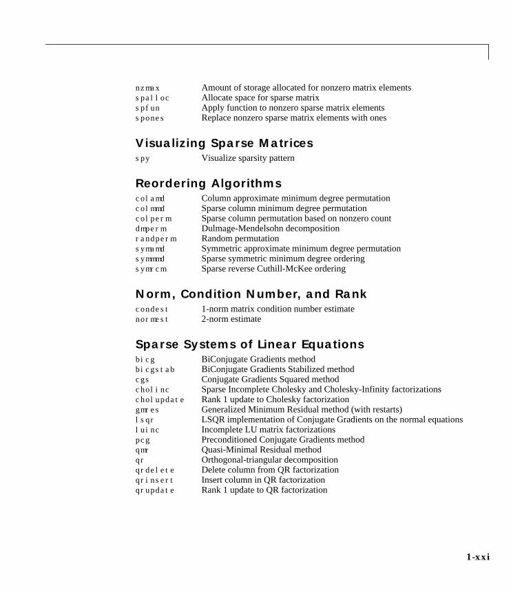
nzmax Amount of storage allocated for nonzero matrix elementsspalloc Allocate space for sparse matrixspfun Apply function to nonzero sparse matrix elementsspones Replace nonzero sparse matrix elements with ones
Visualizing Sparse Matricesspy Visualize sparsity pattern
Reordering Algorithmscolamd Column approximate minimum degree permutationcolmmd Sparse column minimum degree permutationcolperm Sparse column permutation based on nonzero countdmperm Dulmage-Mendelsohn decompositionrandperm Random permutationsymamd Symmetric approximate minimum degree permutationsymmmd Sparse symmetric minimum degree orderingsymrcm Sparse reverse Cuthill-McKee ordering
Norm, Condition Number, and Rankcondest 1-norm matrix condition number estimatenormest 2-norm estimate
Sparse Systems of Linear Equationsbicg BiConjugate Gradients methodbicgstab BiConjugate Gradients Stabilized methodcgs Conjugate Gradients Squared methodcholinc Sparse Incomplete Cholesky and Cholesky-Infinity factorizationscholupdate Rank 1 update to Cholesky factorizationgmres Generalized Minimum Residual method (with restarts)lsqr LSQR implementation of Conjugate Gradients on the normal equationsluinc Incomplete LU matrix factorizationspcg Preconditioned Conjugate Gradients methodqmr Quasi-Minimal Residual methodqr Orthogonal-triangular decompositionqrdelete Delete column from QR factorizationqrinsert Insert column in QR factorizationqrupdate Rank 1 update to QR factorization
1-xxii
Sparse Eigenvalues and Singular Valueseigs Find eigenvalues and eigenvectorssvds Find singular values
Miscellaneousspparms Set parameters for sparse matrix routines
Sound Processing Functions
General Sound Functionslin2mu Convert linear audio signal to mu-lawmu2lin Convert mu-law audio signal to linearsound Convert vector into soundsoundsc Scale data and play as sound
SPARCstation-Specific Sound Functionsauread Read NeXT/SUN (.au) sound fileauwrite Write NeXT/SUN (.au) sound file
.WAV Sound Functionswavplay Play recorded sound on a PC-based audio output devicewavread Read Microsoft WAVE (.wav) sound filewavrecord Record sound using a PC-based audio input devicewavwrite Write Microsoft WAVE (.wav) sound file
Character String Functions
Generalabs Absolute value and complex magnitudeeval Interpret strings containing MATLAB expressionsreal Real part of complex numberstrings MATLAB string handling
String to Function Handle Conversionfunc2str Constructs a function name string from a function handle
1-xxiii
str2func Constructs a function handle from a function name string
String Manipulationdeblank Strip trailing blanks from the end of a stringfindstr Find one string within anotherlower Convert string to lower casestrcat String concatenationstrcmp Compare stringsstrcmpi Compare strings, ignoring casestrjust Justify a character arraystrmatch Find possible matches for a stringstrncmp Compare the firstn characters of stringsstrncmpi Compare the firstn characters of strings, ignoring casestrrep String search and replacestrtok First token in stringstrvcat Vertical concatenation of stringssymvar Determine symbolic variables in an expressiontexlabel Produce the TeX format from a character stringupper Convert string to upper case
String to Number Conversionchar Create character array (string)int2str Integer to string conversionmat2str Convert a matrix into a stringnum2str Number to string conversionsprintf Write formatted data to a stringsscanf Read string under format controlstr2double Convert string to double-precision valuestr2mat String to matrix conversionstr2num String to number conversion
Radix Conversionbin2dec Binary to decimal number conversiondec2bin Decimal to binary number conversiondec2hex Decimal to hexadecimal number conversionhex2dec Hexadecimal to decimal number conversionhex2num Hexadecimal to double number conversion
1-xxiv
File I/O Functions
File Opening and Closingfclose Close one or more open filesfopen Open a file or obtain information about open files
Unformatted I/Ofread Read binary data from filefwrite Write binary data to a file
Formatted I/Ofgetl Return the next line of a file as a string without line terminator(s)fgets Return the next line of a file as a string with line terminator(s)fprintf Write formatted data to filefscanf Read formatted data from file
File Positioningfeof Test for end-of-fileferror Query MATLAB about errors in file input or outputfrewind Rewind an open filefseek Set file position indicatorftell Get file position indicator
String Conversionsprintf Write formatted data to a stringsscanf Read string under format control
Specialized File I/Odlmread Read an ASCII delimited file into a matrixdlmwrite Write a matrix to an ASCII delimited filehdf HDF interfaceimfinfo Return information about a graphics fileimread Read image from graphics fileimwrite Write an image to a graphics filestrread Read formatted data from a stringtextread Read formatted data from text filewk1read Read a Lotus123 WK1 spreadsheet file into a matrix
1-xxv
wk1write Write a matrix to a Lotus123 WK1 spreadsheet file
Bitwise Functionsbitand Bit-wise ANDbitcmp Complement bitsbitor Bit-wise ORbitmax Maximum floating-point integerbitset Set bitbitshift Bit-wise shiftbitget Get bitbitxor Bit-wise XOR
Structure Functionsfieldnames Field names of a structuregetfield Get field of structure arrayrmfield Remove structure fieldssetfield Set field of structure arraystruct Create structure arraystruct2cell Structure to cell array conversion
MATLAB Object Functionsclass Create object or return class of objectisa Detect an object of a given classmethods Display method namesmethodsview Displays information on all methods implemented by a classsubsasgn Overloaded method for A(I)=B, AI=B, and A.field=Bsubsindex Overloaded method for X(A)subsref Overloaded method for A(I), AI and A.field
MATLAB Interface to Javaclass Create object or return class of objectimport Add a package or class to the current Java import listisa Detect an object of a given classisjava Test whether an object is a Java objectjavaArray Constructs a Java array
1-xxvi
javaMethod Invokes a Java methodjavaObject Constructs a Java objectmethods Display method namesmethodsview Displays information on all methods implemented by a class
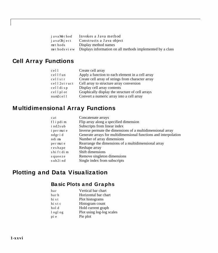
Cell Array Functionscell Create cell arraycellfun Apply a function to each element in a cell arraycellstr Create cell array of strings from character arraycell2struct Cell array to structure array conversioncelldisp Display cell array contentscellplot Graphically display the structure of cell arraysnum2cell Convert a numeric array into a cell array
Multidimensional Array Functionscat Concatenate arraysflipdim Flip array along a specified dimensionind2sub Subscripts from linear indexipermute Inverse permute the dimensions of a multidimensional arrayndgrid Generate arrays for multidimensional functions and interpolationndims Number of array dimensionspermute Rearrange the dimensions of a multidimensional arrayreshape Reshape arrayshiftdim Shift dimensionssqueeze Remove singleton dimensionssub2ind Single index from subscripts
Plotting and Data Visualization
Basic Plots and Graphsbar Vertical bar chartbarh Horizontal bar charthist Plot histogramshistc Histogram counthold Hold current graphloglog Plot using log-log scalespie Pie plot
1-xxvii
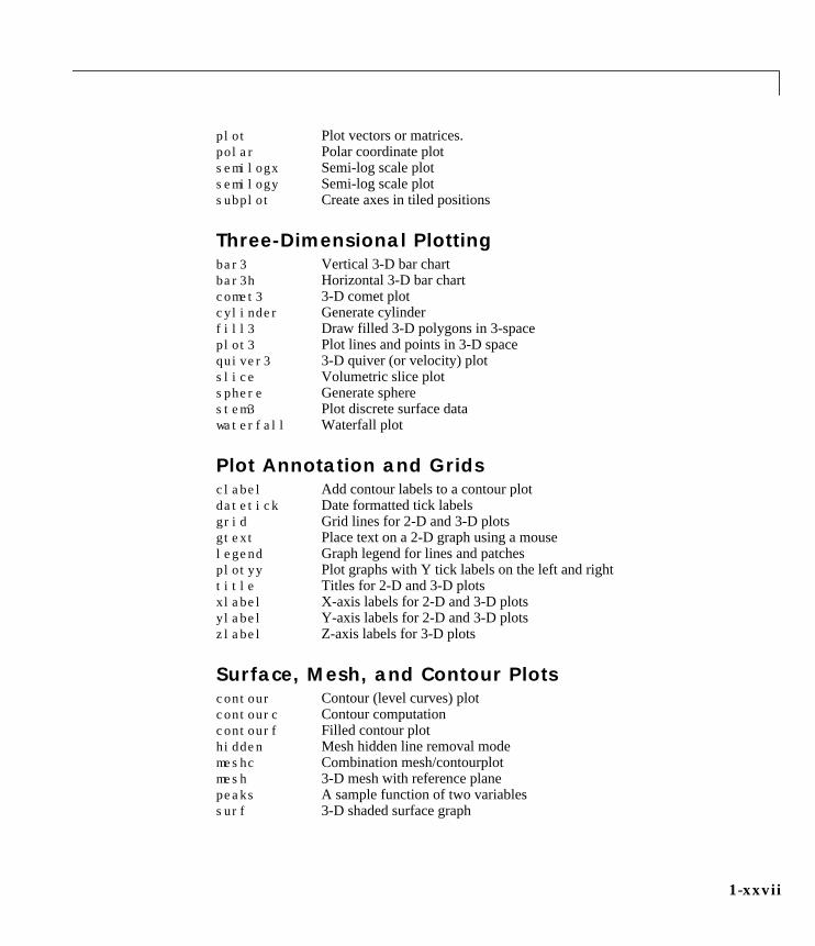
plot Plot vectors or matrices.polar Polar coordinate plotsemilogx Semi-log scale plotsemilogy Semi-log scale plotsubplot Create axes in tiled positions
Three-Dimensional Plottingbar3 Vertical 3-D bar chartbar3h Horizontal 3-D bar chartcomet3 3-D comet plotcylinder Generate cylinderfill3 Draw filled 3-D polygons in 3-spaceplot3 Plot lines and points in 3-D spacequiver3 3-D quiver (or velocity) plotslice Volumetric slice plotsphere Generate spherestem3 Plot discrete surface datawaterfall Waterfall plot
Plot Annotation and Gridsclabel Add contour labels to a contour plotdatetick Date formatted tick labelsgrid Grid lines for 2-D and 3-D plotsgtext Place text on a 2-D graph using a mouselegend Graph legend for lines and patchesplotyy Plot graphs with Y tick labels on the left and righttitle Titles for 2-D and 3-D plotsxlabel X-axis labels for 2-D and 3-D plotsylabel Y-axis labels for 2-D and 3-D plotszlabel Z-axis labels for 3-D plots
Surface, Mesh, and Contour Plotscontour Contour (level curves) plotcontourc Contour computationcontourf Filled contour plothidden Mesh hidden line removal modemeshc Combination mesh/contourplotmesh 3-D mesh with reference planepeaks A sample function of two variablessurf 3-D shaded surface graph
1-xxviii
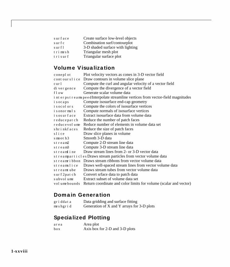
surface Create surface low-level objectssurfc Combination surf/contourplotsurfl 3-D shaded surface with lightingtrimesh Triangular mesh plottrisurf Triangular surface plot
Volume Visualizationconeplot Plot velocity vectors as cones in 3-D vector fieldcontourslice Draw contours in volume slice planecurl Compute the curl and angular velocity of a vector fielddivergence Compute the divergence of a vector fieldflow Generate scalar volume datainterpstreamspeedInterpolate streamline vertices from vector-field magnitudesisocaps Compute isosurface end-cap geometryisocolors Compute the colors of isosurface verticesisonormals Compute normals of isosurface verticesisosurface Extract isosurface data from volume datareducepatch Reduce the number of patch facesreducevolume Reduce number of elements in volume data setshrinkfaces Reduce the size of patch facesslice Draw slice planes in volumesmooth3 Smooth 3-D datastream2 Compute 2-D stream line datastream3 Compute 3-D stream line datastreamline Draw stream lines from 2- or 3-D vector datastreamparticlesDraws stream particles from vector volume datastreamribbon Draws stream ribbons from vector volume datastreamslice Draws well-spaced stream lines from vector volume datastreamtube Draws stream tubes from vector volume datasurf2patch Convert srface data to patch datasubvolume Extract subset of volume data setvolumebounds Return coordinate and color limits for volume (scalar and vector)
Domain Generationgriddata Data gridding and surface fittingmeshgrid Generation of X and Y arrays for 3-D plots
Specialized Plottingarea Area plotbox Axis box for 2-D and 3-D plots
1-xxix
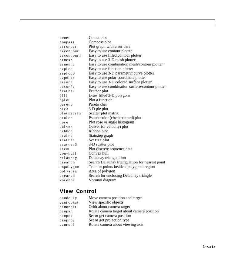
comet Comet plotcompass Compass ploterrorbar Plot graph with error barsezcontour Easy to use contour plotterezcontourf Easy to use filled contour plotterezmesh Easy to use 3-D mesh plotterezmeshc Easy to use combination mesh/contour plotterezplot Easy to use function plotterezplot3 Easy to use 3-D parametric curve plotterezpolar Easy to use polar coordinate plotterezsurf Easy to use 3-D colored surface plotterezsurfc Easy to use combination surface/contour plotterfeather Feather plotfill Draw filled 2-D polygonsfplot Plot a functionpareto Pareto charpie3 3-D pie plotplotmatrix Scatter plot matrixpcolor Pseudocolor (checkerboard) plotrose Plot rose or angle histogramquiver Quiver (or velocity) plotribbon Ribbon plotstairs Stairstep graphscatter Scatter plotscatter3 3-D scatter plotstem Plot discrete sequence dataconvhull Convex hulldelaunay Delaunay triangulationdsearch Search Delaunay triangulation for nearest pointinpolygon True for points inside a polygonal regionpolyarea Area of polygontsearch Search for enclosing Delaunay trianglevoronoi Voronoi diagram
View Controlcamdolly Move camera position and targetcamlookat View specific objectscamorbit Orbit about camera targetcampan Rotate camera target about camera positioncampos Set or get camera positioncamproj Set or get projection typecamroll Rotate camera about viewing axis
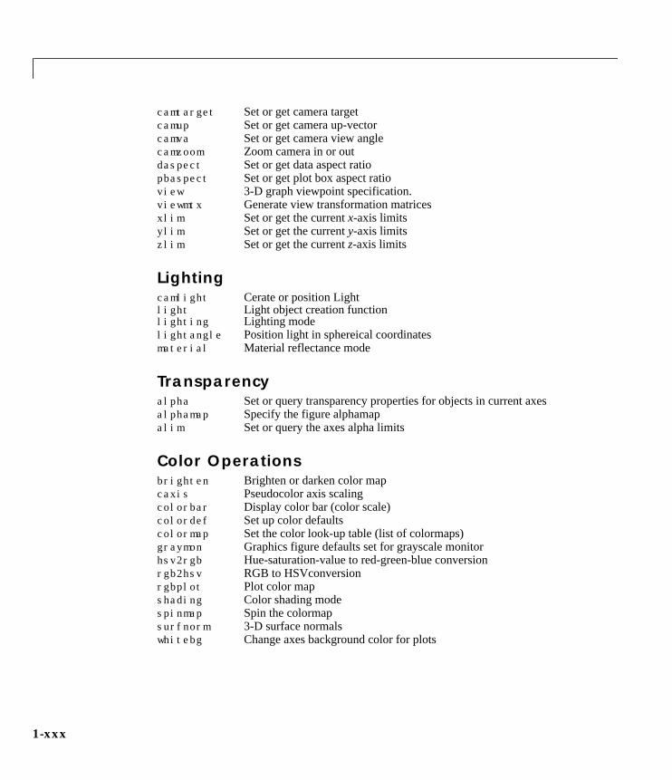
1-xxx
camtarget Set or get camera targetcamup Set or get camera up-vectorcamva Set or get camera view anglecamzoom Zoom camera in or outdaspect Set or get data aspect ratiopbaspect Set or get plot box aspect ratioview 3-D graph viewpoint specification.viewmtx Generate view transformation matricesxlim Set or get the currentx-axis limitsylim Set or get the currenty-axis limitszlim Set or get the currentz-axis limits
Lightingcamlight Cerate or position Lightlight Light object creation functionlighting Lighting modelightangle Position light in sphereical coordinatesmaterial Material reflectance mode
Transparencyalpha Set or query transparency properties for objects in current axesalphamap Specify the figure alphamapalim Set or query the axes alpha limits
Color Operationsbrighten Brighten or darken color mapcaxis Pseudocolor axis scalingcolorbar Display color bar (color scale)colordef Set up color defaultscolormap Set the color look-up table (list of colormaps)graymon Graphics figure defaults set for grayscale monitorhsv2rgb Hue-saturation-value to red-green-blue conversionrgb2hsv RGB to HSVconversionrgbplot Plot color mapshading Color shading modespinmap Spin the colormapsurfnorm 3-D surface normalswhitebg Change axes background color for plots
1-xxxi
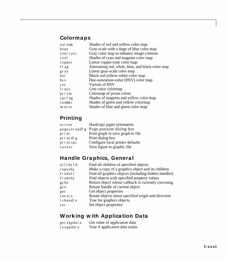
Colormapsautumn Shades of red and yellow color mapbone Gray-scale with a tinge of blue color mapcontrast Gray color map to enhance image contrastcool Shades of cyan and magenta color mapcopper Linear copper-tone color mapflag Alternating red, white, blue, and black color mapgray Linear gray-scale color maphot Black-red-yellow-white color maphsv Hue-saturation-value (HSV) color mapjet Variant of HSVlines Line color colormapprism Colormap of prism colorsspring Shades of magenta and yellow color mapsummer Shades of green and yellow colormapwinter Shades of blue and green color map
Printingorient Hardcopy paper orientationpagesetupdlg Page position dialog boxprint Print graph or save graph to fileprintdlg Print dialog boxprintopt Configure local printer defaultssaveas Save figure to graphic file
Handle Graphics, Generalallchild Find all children of specified objectscopyobj Make a copy of a graphics object and its childrenfindall Find all graphics objects (including hidden handles)findobj Find objects with specified property valuesgcbo Return object whose callback is currently executinggco Return handle of current objectget Get object propertiesrotate Rotate objects about specified origin and directionishandle True for graphics objectsset Set object properties
Working with Application Datagetappdata Get value of application dataisappdata True if application data exists
1-xxxii
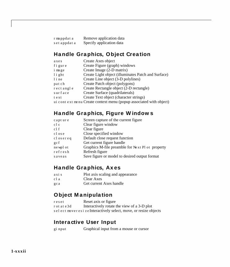
rmappdata Remove application datasetappdata Specify application data
Handle Graphics, Object Creationaxes Create Axes objectfigure Create Figure (graph) windowsimage Create Image (2-D matrix)light Create Light object (illuminates Patch and Surface)line Create Line object (3-D polylines)patch Create Patch object (polygons)rectangle Create Rectangle object (2-D rectangle)surface Create Surface (quadrilaterals)text Create Text object (character strings)uicontextmenuCreate context menu (popup associated with object)
Handle Graphics, Figure Windowscapture Screen capture of the current figureclc Clear figure windowclf Clear figureclose Close specified windowclosereq Default close request functiongcf Get current figure handlenewplot Graphics M-file preamble forNextPlot propertyrefresh Refresh figuresaveas Save figure or model to desired output format
Handle Graphics, Axesaxis Plot axis scaling and appearancecla Clear Axesgca Get current Axes handle
Object Manipulationreset Reset axis or figurerotate3d Interactively rotate the view of a 3-D plotselectmoveresizeInteractively select, move, or resize objects
Interactive User Inputginput Graphical input from a mouse or cursor
1-xxxiii
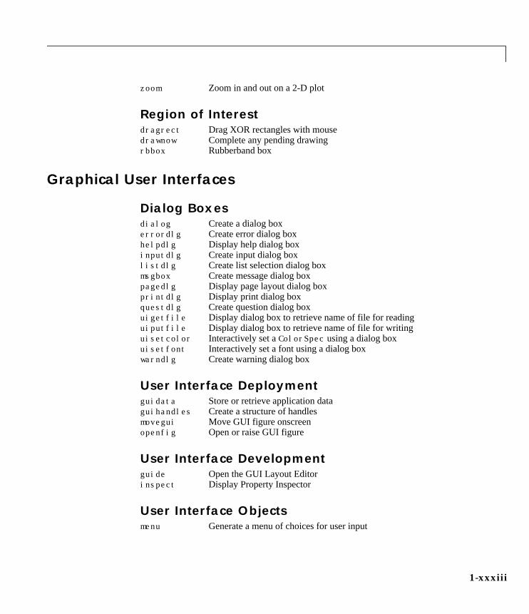
zoom Zoom in and out on a 2-D plot
Region of Interestdragrect Drag XOR rectangles with mousedrawnow Complete any pending drawingrbbox Rubberband box
Graphical User Interfaces
Dialog Boxesdialog Create a dialog boxerrordlg Create error dialog boxhelpdlg Display help dialog boxinputdlg Create input dialog boxlistdlg Create list selection dialog boxmsgbox Create message dialog boxpagedlg Display page layout dialog boxprintdlg Display print dialog boxquestdlg Create question dialog boxuigetfile Display dialog box to retrieve name of file for readinguiputfile Display dialog box to retrieve name of file for writinguisetcolor Interactively set aColorSpec using a dialog boxuisetfont Interactively set a font using a dialog boxwarndlg Create warning dialog box
User Interface Deploymentguidata Store or retrieve application dataguihandles Create a structure of handlesmovegui Move GUI figure onscreenopenfig Open or raise GUI figure
User Interface Developmentguide Open the GUI Layout Editorinspect Display Property Inspector
User Interface Objectsmenu Generate a menu of choices for user input
1-xxxiv
uicontextmenuCreate context menuuicontrol Create user interface controluimenu Create user interface menu
Other Functionsdragrect Drag rectangles with mousefindfigs Display off-screen visible figure windowsgcbf Return handle of figure containing callback objectgcbo Return handle of object whose callback is executingrbbox Create rubberband box for area selectionselectmoveresizeSelect, move, resize, or copy Axes and Uicontrol graphics objectstextwrap Return wrapped string matrix for given Uicontroluiresume Used withuiwait, controls program executionuiwait Used withuiresume, controls program executionwaitbar Display wait barwaitforbuttonpressWait for key/buttonpress over figure
Serial Port I/O
Creating a Serial Port Objectserial Create a serial port object
Writing and Reading Datafgetl Read one line of text from the device and discard the
terminatorfgets Read one line of text from the device and include the
terminatorfprintf Write text to the devicefread Read binary data from the devicefscanf Read data from the device, and format as textfwrite Write binary data to the devicereadasync Read data asynchronously from the devicestopasync Stop asynchronous read and write operations
Configuring and Returning Propertiesget Return serial port object propertiesset Configure or display serial port object properties
1-xxxv
State Changefclose Disconnect a serial port object from the devicefopen Connect a serial port object to the devicerecord Record data and event information to a file
General Purposeclear Remove a serial port object from the MATLAB workspacedelete Remove a serial port object from memorydisp Display serial port object summary informationinstraction Display event information when an event occursinstrfind Return serial port objects from memory to the MATLAB
workspaceisvalid Determine if serial port objects are validlength Length of serial port object arrayload Load serial port objects and variables into the MATLAB
workspacesave Save serial port objects and variables to a MAT-fileserialbreak Send a break to the device connected to the serial portsize Size of serial port object array

1-xxxvi
Volume 3 Reference
Volume 3 Reference
1072
This volume describes the MATLAB operators, special characters, commands,and functions listed alphabetically from P through Z.
Please note that in the three volumes of the MATLAB Function Reference, operatorsand special characters are listed alphabetically according to these categories:
• Arithmetic Operators
• Colon
• Logical Operators
• Special Characters
• Relational Operators
pack
1073
1packPurpose Consolidate workspace memory
Syntax packpack filenamepack('filename')
Description pack frees up needed space by compressing information into the minimummemory required. You must run pack from a directory for which you have writepermission.
pack filename accepts an optional filename for the temporary file used tohold the variables. Otherwise, it uses the file named pack.tmp. You must runpack from a directory for which you have write permission.
pack('filename') is the function form of pack.
Remarks The pack function does not affect the amount of memory allocated to theMATLAB process. You must quit MATLAB to free up this memory.
Since MATLAB uses a heap method of memory management, extendedMATLAB sessions may cause memory to become fragmented. When memory isfragmented, there may be plenty of free space, but not enough contiguousmemory to store a new large variable.
If you get the Out of memory message from MATLAB, the pack function mayfind you some free memory without forcing you to delete variables.
The pack function frees space by:
• Saving all variables on disk in a temporary file called pack.tmp
• Clearing all variables and functions from memory
• Reloading the variables back from pack.tmp
• Deleting the temporary file pack.tmp
If you use pack and there is still not enough free memory to proceed, you mustclear some variables. If you run out of memory often, you can allocate largermatrices earlier in the MATLAB session and use these system-specific tips:
• UNIX: Ask your system manager to increase your swap space.
• Windows: Increase virtual memory using the Windows Control Panel.
pack
1074
Examples Change the current directory to one that is writable, run pack, and return tothe previous directory.
cwd = pwd;cd(tempdir);packcd(cwd)
See Also clear
pagedlg
1075
1pagedlgPurpose This function is obsolete. Use pagesetupdlg to display the page setup dialog.
Syntax pagedlgpagedlg(fig)
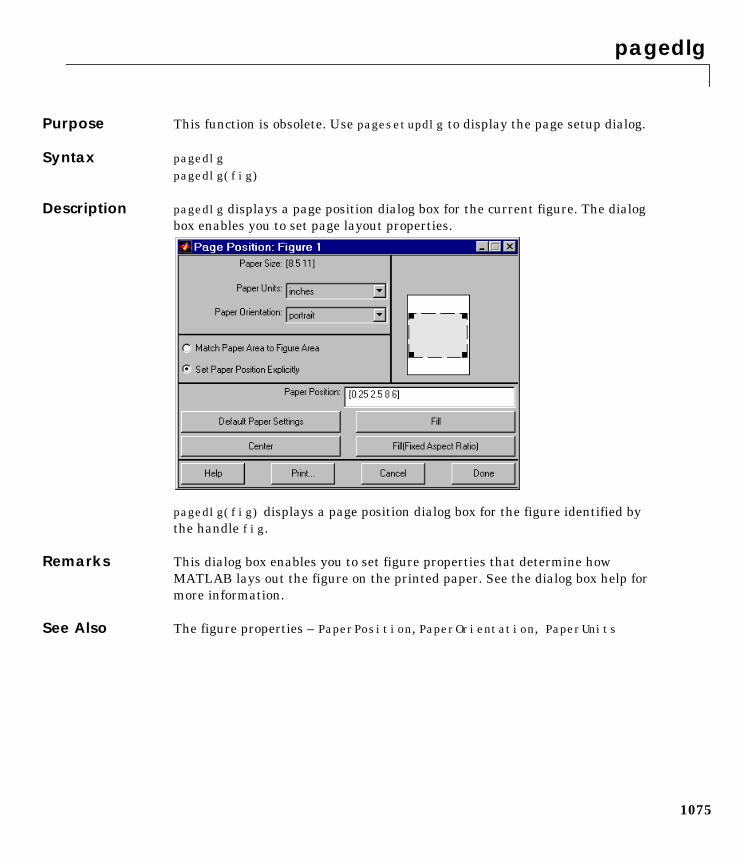
Description pagedlg displays a page position dialog box for the current figure. The dialogbox enables you to set page layout properties.
pagedlg(fig) displays a page position dialog box for the figure identified bythe handle fig.
Remarks This dialog box enables you to set figure properties that determine howMATLAB lays out the figure on the printed paper. See the dialog box help formore information.
See Also The figure properties – PaperPosition, PaperOrientation, PaperUnits
pagesetupdlg
1076
1pagesetupdlgPurpose Page position dialog box
Syntax dlg = pagesetupdlg(fig)
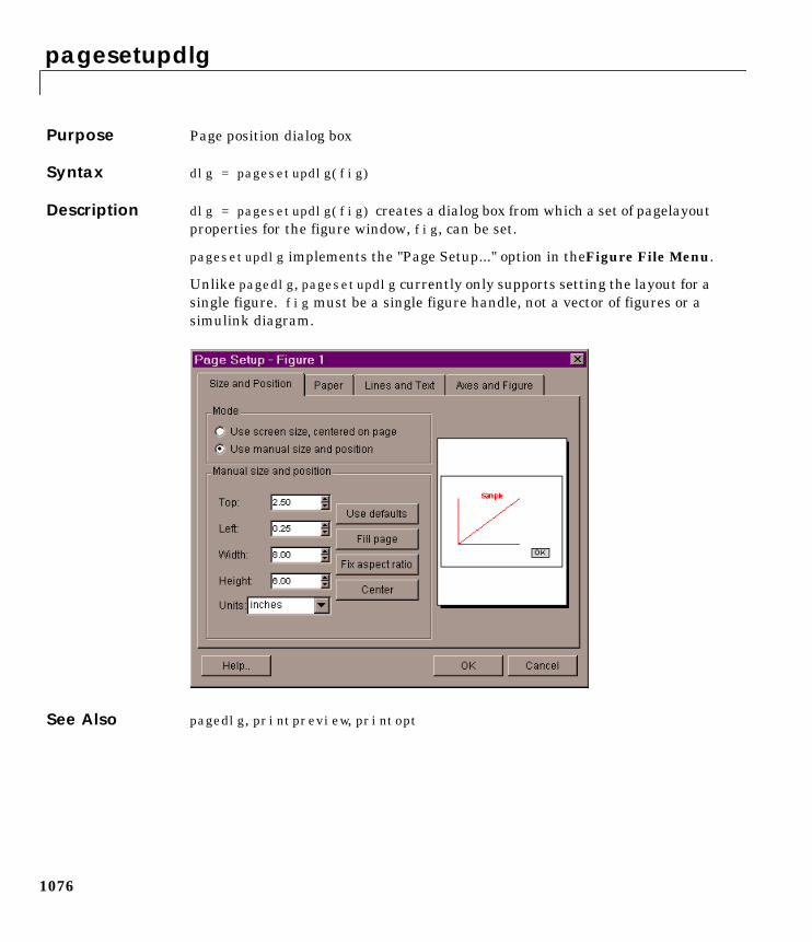
Description dlg = pagesetupdlg(fig) creates a dialog box from which a set of pagelayoutproperties for the figure window, fig, can be set.
pagesetupdlg implements the "Page Setup..." option in theFigure File Menu.
Unlike pagedlg, pagesetupdlg currently only supports setting the layout for asingle figure. fig must be a single figure handle, not a vector of figures or asimulink diagram.
See Also pagedlg, printpreview, printopt
pareto
1077
1paretoPurpose Pareto chart
Syntax pareto(Y)pareto(Y,names)pareto(Y,X)H = pareto(...)
Description Pareto charts display the values in the vector Y as bars drawn in descendingorder.
pareto(Y) labels each bar with its element index in Y.
pareto(Y,names) labels each bar with the associated name in the string matrixor cell array names.
pareto(Y,X) labels each bar with the associated value from X.
H = pareto(...) returns a combination of patch and line object handles.
See Also hist, bar
partialpath
1078
1partialpathPurpose Partial pathname
Description A partial pathname is a pathname relative to the MATLAB path, MATLABPATH.It is used to locate private and method files, which are usually hidden, or torestrict the search for files when more than one file with the given name exists.
A partial pathname contains the last component, or last several components,of the full pathname separated by /. For example, matfun/trace,private/children, inline/formula, and demos/clown.mat are valid partialpathnames. Specifying the @ in method directory names is optional, sofunfun/inline/formula is also a valid partial pathname.
Partial pathnames make it easy to find toolbox or MATLAB relative files onyour path in a portable way, independent of the location where MATLAB isinstalled.
Many commands accept partial pathnames instead of a full pathname. Some ofthese commands are
help, type, load, exist, what, which, edit, dbtype, dbstop,dbclear, and fopen
Examples The following examples use partial pathnames.
what funfun/inline
M-files in directory matlabroot\toolbox\matlab\funfun\@inlineargnames disp feval inline subsref vertcatcat display formula nargin symvarchar exist horzcat nargout vectorize
which funfun/inline/formulamatlabroot\toolbox\matlab\funfun\@inline\formula.m% inline method
See Also path
pascal
1079
1pascalPurpose Pascal matrix
Syntax A = pascal(n)A = pascal(n,1)A = pascal(n,2)
Description A = pascal(n) returns the Pascal matrix of order n: a symmetric positivedefinite matrix with integer entries taken from Pascal’s triangle. The inverseof A has integer entries.
A = pascal(n,1) returns the lower triangular Cholesky factor (up to the signsof the columns) of the Pascal matrix. It is involutary, that is, it is its owninverse.
A = pascal(n,2) returns a transposed and permuted version of pascal(n,1).A is a cube root of the identity matrix.
Examples pascal(4) returns
1 1 1 11 2 3 41 3 6 101 4 10 20
A = pascal(3,2) produces
A = 0 0 -1 0 -1 2 -1 -1 1
See Also chol
patch
1080
1patchPurpose Create patch graphics object
Syntax patch(X,Y,C)patch(X,Y,Z,C)patch(FV)patch(...'PropertyName',PropertyValue...)patch('PropertyName',PropertyValue...) PN/PV pairs onlyhandle = patch(...)
Description patch is the low-level graphics function for creating patch graphics objects. Apatch object is one or more polygons defined by the coordinates of its vertices.You can specify the coloring and lighting of the patch. See the Creating 3-DModels with Patches for more information on using patch objects.
patch(X,Y,C) adds the filled two-dimensional patch to the current axes. Theelements of X and Y specify the vertices of a polygon. If X and Y are matrices,MATLAB draws one polygon per column. C determines the color of the patch.It can be a single ColorSpec, one color per face, or one color per vertex (see“Remarks”). If C is a 1-by-3 vector, it is assumed to be an RGB triplet,specifying a color directly.
patch(X,Y,Z,C) creates a patch in three-dimensional coordinates.
patch(FV) creates a patch using structure FV, which contains the fieldsvertices, faces, and optionally facevertecdata. These fields correspond tothe Vertices, Faces, and FaceVertexCData patch properties.
patch(...'PropertyName',PropertyValue...) follows the X, Y, (Z), and Carguments with property name/property value pairs to specify additional patchproperties.
patch('PropertyName',PropertyValue,...) specifies all properties usingproperty name/property value pairs. This form enables you to omit the colorspecification because MATLAB uses the default face color and edge color,unless you explicitly assign a value to the FaceColor and EdgeColorproperties. This form also allows you to specify the patch using the Faces andVertices properties instead of x-, y-, and z-coordinates. See the “Examples”section for more information.
patch
1081
handle = patch(...) returns the handle of the patch object it creates.
Remarks Unlike high-level area creation functions, such as fill or area, patch does notcheck the settings of the figure and axes NextPlot properties. It simply adds thepatch object to the current axes.
If the coordinate data does not define closed polygons, patch closes thepolygons. The data can define concave or intersecting polygons. However, if theedges of an individual patch face intersect themselves, the resulting face mayor may not be completely filled. In that case, it is better to break up the face intosmaller polygons.
Specifying Patch PropertiesYou can specify properties as property name/property value pairs, structurearrays, and cell arrays (see the set and get reference pages for examples of howto specify these data types).
There are two patch properties that specify color:
• CData – use when specifying x-, y-, and z-coordinates (XData, YData, ZData).
• FaceVertexCData – use when specifying vertices and connection matrix(Vertices and Faces).
The CData and FaceVertexCData properties accept color data as indexed or truecolor (RGB) values. See the CData and FaceVertexCData property descriptionsfor information on how to specify color.
Indexed color data can represent either direct indices into the colormap orscaled values that map the data linearly to the entire colormap (see the caxis
patch
1082
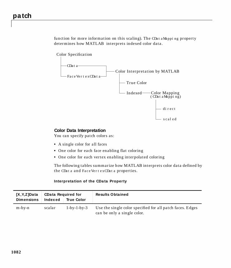
function for more information on this scaling). The CDataMapping propertydetermines how MATLAB interprets indexed color data.
Color Data InterpretationYou can specify patch colors as:
• A single color for all faces
• One color for each face enabling flat coloring
• One color for each vertex enabling interpolated coloring
The following tables summarize how MATLAB interprets color data defined bythe CData and FaceVertexCData properties.
Interpretation of the CData Property
Color Specification
FaceVertexCData
CData
Indexed
True Color
direct
scaled
(CDataMapping)
Color Interpretation by MATLAB
Color Mapping
[X,Y,Z]Data CData Required for Results ObtainedDimensions Indexed True Color
m-by-n scalar 1-by-1-by-3 Use the single color specified for all patch faces. Edgescan be only a single color.
patch
1083
Interpretation of the FaceVertexCData Property
Examples This example creates a patch object using two different methods:
• Specifying x-, y-, and z-coordinates and color data (XData, YData, ZData, andCData properties).
• Specifying vertices, the connection matrix, and color data (Vertices, Faces,FaceVertexCData, and FaceColor properties).
m-by-n 1-by-n(n >= 4)
1-by-n-by-3 Use one color for each patch face. Edges can be only asingle color.
m-by-n m-by-n m-by-n-3 Assign a color to each vertex. patch faces can be flat (asingle color) or interpolated. Edges can be flat orinterpolated.
[X,Y,Z]Data CData Required for Results ObtainedDimensions Indexed True Color
Vertices Faces FaceVertexCDataRequired for
Results Obtained
Dimensions Dimensions Indexed True Color
m-by-n k-by-3 scalar 1-by-3 Use the single color specified for allpatch faces. Edges can be only a singlecolor.
m-by-n k-by-3 k-by-1 k-by-3 Use one color for each patch face. Edgescan be only a single color.
m-by-n k-by-3 m-by-1 m-by-3 Assign a color to each vertex. patch facescan be flat (a single color) orinterpolated. Edges can be flat orinterpolated.
patch
1084
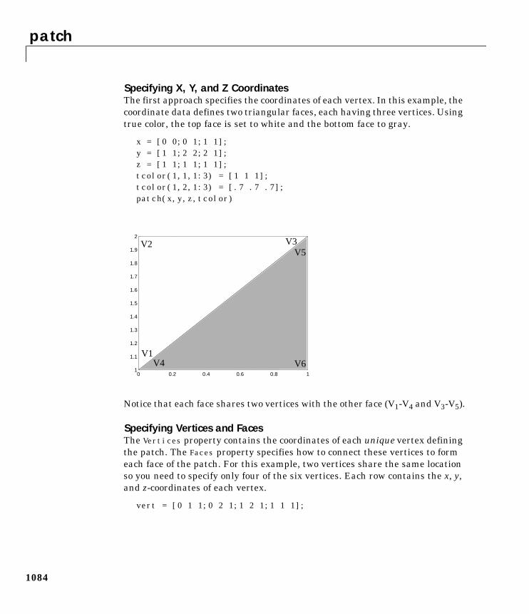
Specifying X, Y, and Z CoordinatesThe first approach specifies the coordinates of each vertex. In this example, thecoordinate data defines two triangular faces, each having three vertices. Usingtrue color, the top face is set to white and the bottom face to gray.
x = [0 0;0 1;1 1];y = [1 1;2 2;2 1];z = [1 1;1 1;1 1];tcolor(1,1,1:3) = [1 1 1];tcolor(1,2,1:3) = [.7 .7 .7];patch(x,y,z,tcolor)
Notice that each face shares two vertices with the other face (V1-V4 and V3-V5).
Specifying Vertices and FacesThe Vertices property contains the coordinates of each unique vertex definingthe patch. The Faces property specifies how to connect these vertices to formeach face of the patch. For this example, two vertices share the same locationso you need to specify only four of the six vertices. Each row contains the x, y,and z-coordinates of each vertex.
vert = [0 1 1;0 2 1;1 2 1;1 1 1];
0 0.2 0.4 0.6 0.8 11
1.1
1.2
1.3
1.4
1.5
1.6
1.7
1.8
1.9
2
V2 V3V5
V6V1
V4
patch
1085
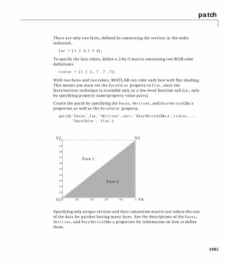
There are only two faces, defined by connecting the vertices in the orderindicated.
fac = [1 2 3;1 3 4];
To specify the face colors, define a 2-by-3 matrix containing two RGB colordefinitions.
tcolor = [1 1 1;.7 .7 .7];
With two faces and two colors, MATLAB can color each face with flat shading.This means you must set the FaceColor property to flat, since thefaces/vertices technique is available only as a low-level function call (i.e., onlyby specifying property name/property value pairs).
Create the patch by specifying the Faces, Vertices, and FaceVertexCDataproperties as well as the FaceColor property.
patch('Faces',fac,'Vertices',vert,'FaceVertexCData',tcolor,...'FaceColor','flat')
Specifying only unique vertices and their connection matrix can reduce the sizeof the data for patches having many faces. See the descriptions of the Faces,Vertices, and FaceVertexCData properties for information on how to definethem.
0 0.2 0.4 0.6 0.8 11
1.1
1.2
1.3
1.4
1.5
1.6
1.7
1.8
1.9
2
V1
V2 V3
V4
Face 1
Face 2
patch
1086
MATLAB does not require each face to have the same number of vertices. Incases where they do not, pad the Faces matrix with NaNs. To define a patchwith faces that do not close, add one or more NaN to the row in the Verticesmatrix that defines the vertex you do not want connected.
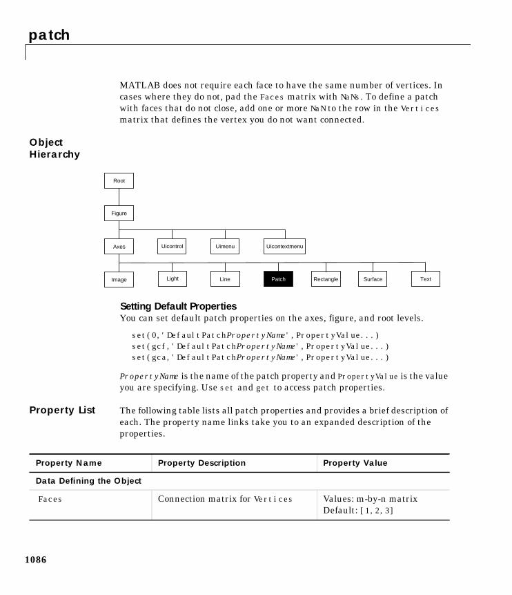
ObjectHierarchy
Setting Default PropertiesYou can set default patch properties on the axes, figure, and root levels.
set(0,'DefaultPatchPropertyName',PropertyValue...)set(gcf,'DefaultPatchPropertyName',PropertyValue...)set(gca,'DefaultPatchPropertyName',PropertyValue...)
PropertyName is the name of the patch property and PropertyValue is the valueyou are specifying. Use set and get to access patch properties.
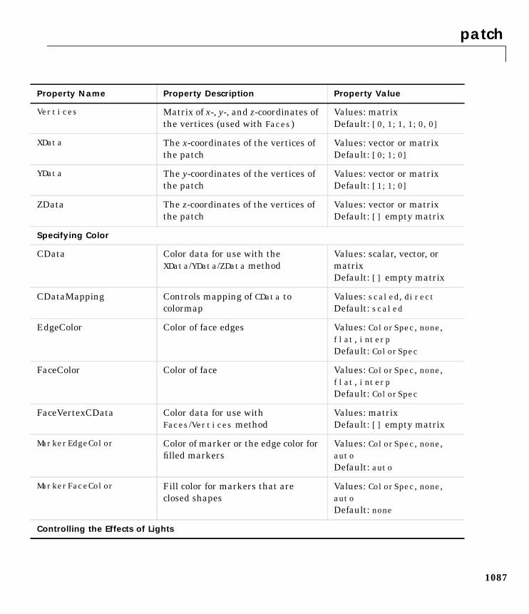
Property List The following table lists all patch properties and provides a brief description ofeach. The property name links take you to an expanded description of theproperties.
Uimenu
Line
Axes Uicontrol
Image
Figure
Uicontextmenu
Light SurfacePatch Text
Root
Rectangle
Property Name Property Description Property Value
Data Defining the Object
Faces Connection matrix for Vertices Values: m-by-n matrixDefault: [1,2,3]
patch
1087
Vertices Matrix of x-, y-, and z-coordinates ofthe vertices (used with Faces)
Values: matrixDefault: [0,1;1,1;0,0]
XData The x-coordinates of the vertices ofthe patch
Values: vector or matrixDefault: [0;1;0]
YData The y-coordinates of the vertices ofthe patch
Values: vector or matrixDefault: [1;1;0]
ZData The z-coordinates of the vertices ofthe patch
Values: vector or matrixDefault: [] empty matrix
Specifying Color
CData Color data for use with theXData/YData/ZData method
Values: scalar, vector, ormatrixDefault: [] empty matrix
CDataMapping Controls mapping of CData tocolormap
Values: scaled, directDefault: scaled
EdgeColor Color of face edges Values: ColorSpec, none,flat, interpDefault: ColorSpec
FaceColor Color of face Values: ColorSpec, none,flat, interpDefault: ColorSpec
FaceVertexCData Color data for use withFaces/Vertices method
Values: matrixDefault: [] empty matrix
MarkerEdgeColor Color of marker or the edge color forfilled markers
Values: ColorSpec, none,autoDefault: auto
MarkerFaceColor Fill color for markers that areclosed shapes
Values: ColorSpec, none,autoDefault: none
Controlling the Effects of Lights
Property Name Property Description Property Value
patch
1088
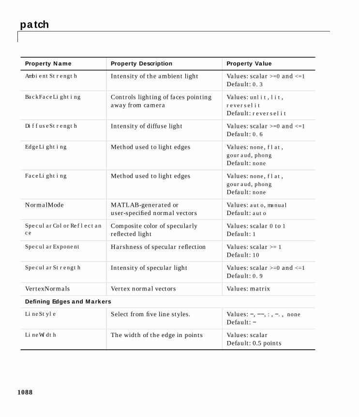
AmbientStrength Intensity of the ambient light Values: scalar >=0 and <=1Default: 0.3
BackFaceLighting Controls lighting of faces pointingaway from camera
Values: unlit, lit,reverselitDefault: reverselit
DiffuseStrength Intensity of diffuse light Values: scalar >=0 and <=1Default: 0.6
EdgeLighting Method used to light edges Values: none, flat,gouraud, phongDefault: none
FaceLighting Method used to light edges Values: none, flat,gouraud, phongDefault: none
NormalMode MATLAB-generated oruser-specified normal vectors
Values: auto, manualDefault: auto
SpecularColorReflectance
Composite color of specularlyreflected light
Values: scalar 0 to 1Default: 1
SpecularExponent Harshness of specular reflection Values: scalar >= 1Default: 10
SpecularStrength Intensity of specular light Values: scalar >=0 and <=1Default: 0.9
VertexNormals Vertex normal vectors Values: matrix
Defining Edges and Markers
LineStyle Select from five line styles. Values: −, −−, :, −., noneDefault: −
LineWidth The width of the edge in points Values: scalarDefault: 0.5 points
Property Name Property Description Property Value
patch
1089
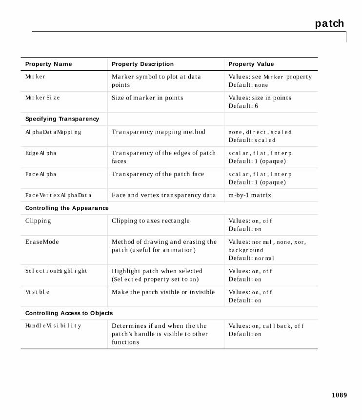
Marker Marker symbol to plot at datapoints
Values: see Marker propertyDefault: none
MarkerSize Size of marker in points Values: size in pointsDefault: 6
Specifying Transparency
AlphaDataMapping Transparency mapping method none, direct, scaledDefault: scaled
EdgeAlpha Transparency of the edges of patchfaces
scalar, flat, interpDefault: 1 (opaque)
FaceAlpha Transparency of the patch face scalar, flat, interpDefault: 1 (opaque)
FaceVertexAlphaData Face and vertex transparency data m-by-1 matrix
Controlling the Appearance
Clipping Clipping to axes rectangle Values: on, offDefault: on
EraseMode Method of drawing and erasing thepatch (useful for animation)
Values: normal, none, xor,backgroundDefault: normal
SelectionHighlight Highlight patch when selected(Selected property set to on)
Values: on, offDefault: on
Visible Make the patch visible or invisible Values: on, offDefault: on
Controlling Access to Objects
HandleVisibility Determines if and when the thepatch’s handle is visible to otherfunctions
Values: on, callback, offDefault: on
Property Name Property Description Property Value
patch
1090
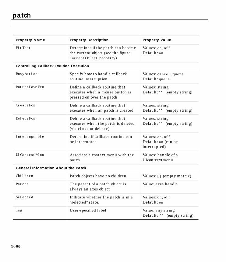
HitTest Determines if the patch can becomethe current object (see the figureCurrentObject property)
Values: on, offDefault: on
Controlling Callback Routine Execution
BusyAction Specify how to handle callbackroutine interruption
Values: cancel, queueDefault: queue
ButtonDownFcn Define a callback routine thatexecutes when a mouse button ispressed on over the patch
Values: stringDefault: '' (empty string)
CreateFcn Define a callback routine thatexecutes when an patch is created
Values: stringDefault: '' (empty string)
DeleteFcn Define a callback routine thatexecutes when the patch is deleted(via close or delete)
Values: stringDefault: '' (empty string)
Interruptible Determine if callback routine canbe interrupted
Values: on, offDefault: on (can beinterrupted)
UIContextMenu Associate a context menu with thepatch
Values: handle of aUicontrextmenu
General Information About the Patch
Children Patch objects have no children Values: [] (empty matrix)
Parent The parent of a patch object isalways an axes object
Value: axes handle
Selected Indicate whether the patch is in a“selected” state.
Values: on, offDefault: on
Tag User-specified label Value: any stringDefault: '' (empty string)
Property Name Property Description Property Value
patch
1091
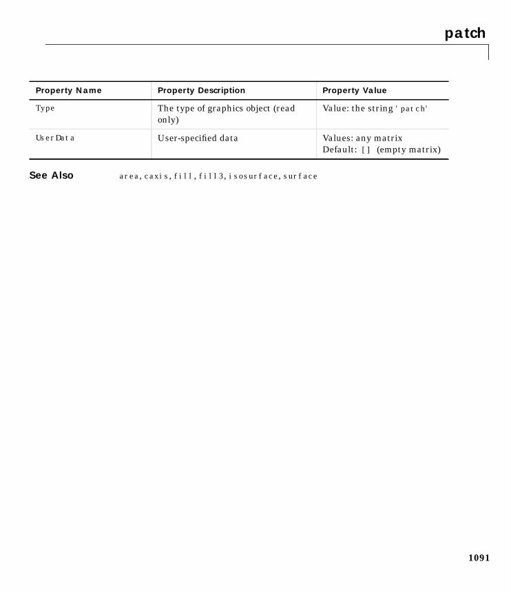
See Also area, caxis, fill, fill3, isosurface, surface
Type The type of graphics object (readonly)
Value: the string 'patch'
UserData User-specified data Values: any matrixDefault: [] (empty matrix)
Property Name Property Description Property Value
Patch Properties
1092
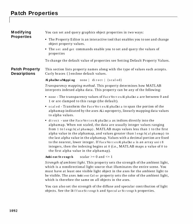
1Patch PropertiesModifyingProperties
You can set and query graphics object properties in two ways:
• The Property Editor is an interactive tool that enables you to see and changeobject property values.
• The set and get commands enable you to set and query the values ofproperties
To change the default value of properties see Setting Default Property Values.
Patch PropertyDescriptions
This section lists property names along with the type of values each accepts.Curly braces enclose default values.
AlphaDataMapping none | direct | scaled
Transparency mapping method. This property determines how MATLABinterprets indexed alpha data. This property can be any of the following:
• none - The transparency values of FaceVertexAlphaData are between 0 and1 or are clamped to this range (the default).
• scaled - Transform the FaceVertexAlphaData to span the portion of thealphamap indicated by the axes ALim property, linearly mapping data valuesto alpha values.
• direct - use the FaceVertexAlphaData as indices directly into thealphamap. When not scaled, the data are usually integer values rangingfrom 1 to length(alphamap). MATLAB maps values less than 1 to the firstalpha value in the alphamap, and values greater than length(alphamap) tothe last alpha value in the alphamap. Values with a decimal portion are fixedto the nearest, lower integer. If FaceVertexAlphaData is an array unit8integers, then the indexing begins at 0 (i.e., MATLAB maps a value of 0 tothe first alpha value in the alphamap).
AmbientStrength scalar >= 0 and <= 1
Strength of ambient light. This property sets the strength of the ambient light,which is a nondirectional light source that illuminates the entire scene. Youmust have at least one visible light object in the axes for the ambient light tobe visible. The axes AmbientColor property sets the color of the ambient light,which is therefore the same on all objects in the axes.
You can also set the strength of the diffuse and specular contribution of lightobjects. See the DiffuseStrength and SpecularStrength properties.
Patch Properties
1093
BackFaceLighting unlit | lit | reverselit
Face lighting control. This property determines how faces are lit when theirvertex normals point away from the camera:
• unlit – face is not lit
• lit – face lit in normal way
• reverselit – face is lit as if the vertex pointed towards the camera
This property is useful for discriminating between the internal and externalsurfaces of an object. See the Using MATLAB Graphics manual for an example.
BusyAction cancel | queue
Callback routine interruption. The BusyAction property enables you to controlhow MATLAB handles events that potentially interrupt executing callbackroutines. If there is a callback routine executing, subsequently invokedcallback routes always attempt to interrupt it. If the Interruptible propertyof the object whose callback is executing is set to on (the default), theninterruption occurs at the next point where the event queue is processed. If theInterruptible property is off, the BusyAction property (of the object owningthe executing callback) determines how MATLAB handles the event. Thechoices are:
• cancel – discard the event that attempted to execute a second callbackroutine.
• queue – queue the event that attempted to execute a second callback routineuntil the current callback finishes.
ButtonDownFcn string
Button press callback routine. A callback routine that executes whenever youpress a mouse button while the pointer is over the patch object. Define thisroutine as a string that is a valid MATLAB expression or the name of an M-file.The expression executes in the MATLAB workspace.
CData scalar, vector, or matrix
Patch colors. This property specifies the color of the patch. You can specify colorfor each vertex, each face, or a single color for the entire patch. The wayMATLAB interprets CData depends on the type of data supplied. The data canbe numeric values that are scaled to map linearly into the current colormap,integer values that are used directly as indices into the current colormap, or
Patch Properties
1094
arrays of RGB values. RGB values are not mapped into the current colormap,but interpreted as the colors defined. On true color systems, MATLAB uses theactual colors defined by the RGB triples. On pseudocolor systems, MATLABuses dithering to approximate the RGB triples using the colors in the figure’sColormap and Dithermap.
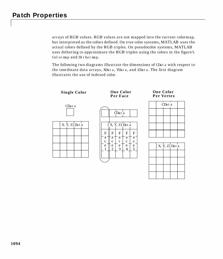
The following two diagrams illustrate the dimensions of CData with respect tothe coordinate data arrays, XData, YData, and ZData. The first diagramillustrates the use of indexed color.
Single Color
CData
[X,Y,Z]Data
Face1
Face2
Face3
Face4
Face5
One ColorPer Face
CData
One ColorPer Vertex
CData
[X,Y,Z]Data
[X,Y,Z]Data
Patch Properties
1095
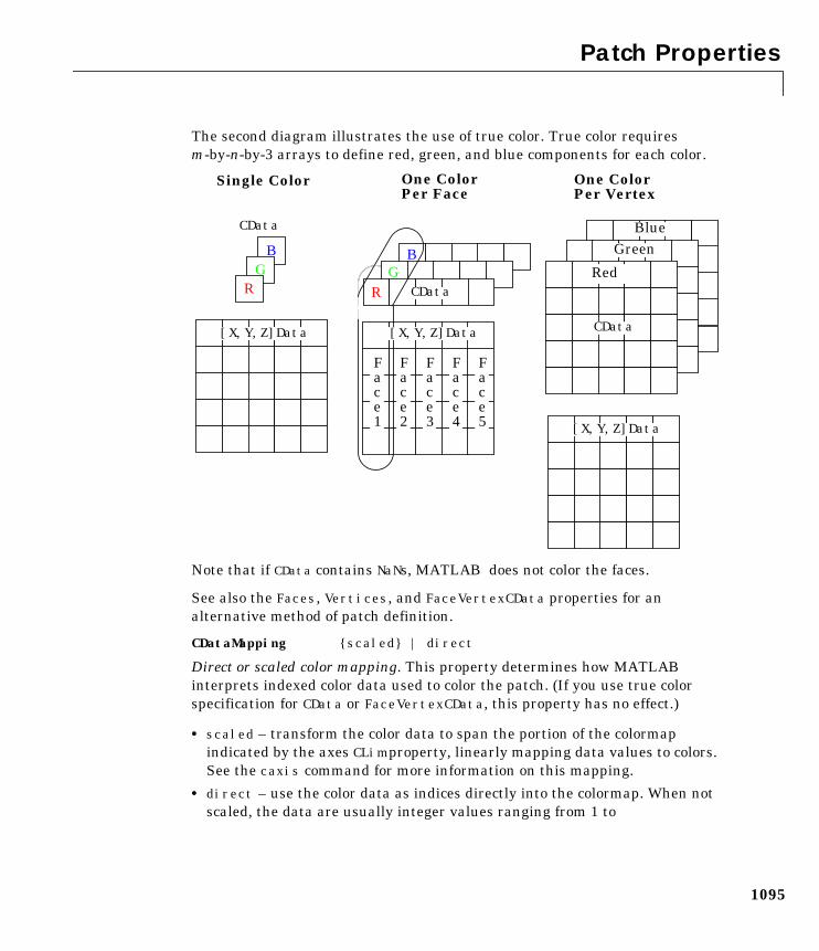
The second diagram illustrates the use of true color. True color requiresm-by-n-by-3 arrays to define red, green, and blue components for each color.
Note that if CData contains NaNs, MATLAB does not color the faces.
See also the Faces, Vertices, and FaceVertexCData properties for analternative method of patch definition.
CDataMapping scaled | direct
Direct or scaled color mapping. This property determines how MATLABinterprets indexed color data used to color the patch. (If you use true colorspecification for CData or FaceVertexCData, this property has no effect.)
• scaled – transform the color data to span the portion of the colormapindicated by the axes CLim property, linearly mapping data values to colors.See the caxis command for more information on this mapping.
• direct – use the color data as indices directly into the colormap. When notscaled, the data are usually integer values ranging from 1 to
Single Color One ColorPer Face
One ColorPer Vertex
BG
R
CData
Face1
Face2
Face3
Face4
Face5
RG
B
CDataRed
GreenBlue
CData
[X,Y,Z]Data
[X,Y,Z]Data [X,Y,Z]Data
Patch Properties
1096
length(colormap). MATLAB maps values less than 1 to the first color in thecolormap, and values greater than length(colormap) to the last color in thecolormap. Values with a decimal portion are fixed to the nearest, lowerinteger.
Children matrix of handles
Always the empty matrix; patch objects have no children.
Clipping on | off
Clipping to axes rectangle. When Clipping is on, MATLAB does not display anyportion of the patch outside the axes rectangle.
CreateFcn string
Callback routine executed during object creation. This property defines acallback routine that executes when MATLAB creates a patch object. Youmust define this property as a default value for patches. For example, thestatement,
set(0,'DefaultPatchCreateFcn','set(gcf,''DitherMap'',my_dither_map)')
defines a default value on the root level that sets the figure DitherMap propertywhenever you create a patch object. MATLAB executes this routine aftersetting all properties for the patch created. Setting this property on an existingpatch object has no effect.
The handle of the object whose CreateFcn is being executed is accessible onlythrough the root CallbackObject property, which you can query using gcbo.
DeleteFcn string
Delete patch callback routine. A callback routine that executes when you deletethe patch object (e.g., when you issue a delete command or clear the axes (cla)or figure (clf) containing the patch). MATLAB executes the routine beforedeleting the object’s properties so these values are available to the callbackroutine.
The handle of the object whose DeleteFcn is being executed is accessible onlythrough the root CallbackObject property, which you can query using gcbo.
Patch Properties
1097
DiffuseStrength scalar >= 0 and <= 1
Intensity of diffuse light. This property sets the intensity of the diffusecomponent of the light falling on the patch. Diffuse light comes from lightobjects in the axes.
You can also set the intensity of the ambient and specular components of thelight on the patch object. See the AmbientStrength and SpecularStrengthproperties.
EdgeAlpha scalar = 1 | flat | interp
Transparency of the edges of patch faces. This property can be any of thefollowing:
• scalar - A single non-Nan scalar value between 0 and 1 that controls thetransparency of all the edges of the object. 1 (the default) is fully opaque and0 means completely transparent.
• flat - The alpha data (FaceVertexAlphaData) of each vertex controls thetransparency of the edge that follows it.
• interp - Linear interpolation of the alpha data (FaceVertexAlphaData) ateach vertex determines the transparency of the edge.
Note that you cannot specify flat or interp EdgeAlpha without first settingFaceVertexAlphaData to a matrix containing one alpha value per face (flat) orone alpha value per vertex (interp).
EdgeColor ColorSpec | none | flat | interp
Color of the patch edge. This property determines how MATLAB colors theedges of the individual faces that make up the patch.
• ColorSpec – A three-element RGB vector or one of MATLAB’s predefinednames, specifying a single color for edges. The default edge color is black. SeeColorSpec for more information on specifying color.
• none – Edges are not drawn.
Patch Properties
1098
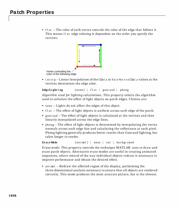
• flat – The color of each vertex controls the color of the edge that follows it.This means flat edge coloring is dependent on the order you specify thevertices:
• interp – Linear interpolation of the CData or FaceVertexCData values at thevertices determines the edge color.
EdgeLighting none | flat | gouraud | phong
Algorithm used for lighting calculations. This property selects the algorithmused to calculate the effect of light objects on patch edges. Choices are:
• none – Lights do not affect the edges of this object.
• flat – The effect of light objects is uniform across each edge of the patch.
• gouraud – The effect of light objects is calculated at the vertices and thenlinearly interpolated across the edge lines.
• phong – The effect of light objects is determined by interpolating the vertexnormals across each edge line and calculating the reflectance at each pixel.Phong lighting generally produces better results than Gouraud lighting, buttakes longer to render.
EraseMode normal | none | xor | background
Erase mode. This property controls the technique MATLAB uses to draw anderase patch objects. Alternative erase modes are useful in creating animatedsequences, where control of the way individual objects redraw is necessary toimprove performance and obtain the desired effect.
• normal – Redraw the affected region of the display, performing thethree-dimensional analysis necessary to ensure that all objects are renderedcorrectly. This mode produces the most accurate picture, but is the slowest.
Vertex controlling thecolor of the following edge
Patch Properties
1099
The other modes are faster, but do not perform a complete redraw and aretherefore less accurate.
• none – Do not erase the patch when it is moved or destroyed. While the objectis still visible on the screen after erasing with EraseMode none, you cannotprint it because MATLAB stores no information about its former location.
• xor– Draw and erase the patch by performing an exclusive OR (XOR) witheach pixel index of the screen behind it. Erasing the patch does not damagethe color of the objects behind it. However, patch color depends on the colorof the screen behind it and is correctly colored only when over the axesbackground Color, or the figure background Color if the axes Color is set tonone.
• background – Erase the patch by drawing it in the axes’ background Color,or the figure background Color if the axes Color is set to none. This damagesobjects that are behind the erased patch, but the patch is always properlycolored.
Printing with Non-normal Erase Modes. MATLAB always prints figures as if theEraseMode of all objects is normal. This means graphics objects created withEraseMode set to none, xor, or background can look different on screen than onpaper. On screen, MATLAB may mathematically combine layers of colors (e.g.,XORing a pixel color with that of the pixel behind it) and ignorethree-dimensional sorting to obtain greater rendering speed. However, thesetechniques are not applied to the printed output.
You can use the MATLAB getframe command or other screen captureapplication to create an image of a figure containing non-normal mode objects.
FaceAlpha scalar = 1 | flat | interp
Transparency of the patch face. This property can be any of the following:
• A scalar - A single non-NaN scalar value between 0 and 1 that controls thetransparency of all the faces of the object. 1 (the default) is fully opaque and0 is completely transparent (invisible).
• flat - The values of the alpha data (FaceVertexAlphaData) determine thetransparency for each face. The alpha data at the first vertex determines thetransparency of the entire face.
• interp - Bilinear interpolation of the alpha data (FaceVertexAlphaData) ateach vertex determine the transparency of each face.
Patch Properties
1100
Note that you cannot specify flat or interp FaceAlpha without first settingFaceVertexAlphaData to a matrix containing one alpha value per face (flat)or one alpha value per vertex (interp).
FaceColor ColorSpec | none | flat | interp
Color of the patch face. This property can be any of the following:
• ColorSpec – A three-element RGB vector or one of MATLAB’s predefinednames, specifying a single color for faces. See ColorSpec for moreinformation on specifying color.
• none – Do not draw faces. Note that edges are drawn independently of faces.
• flat – The values of CData or FaceVertexCData determine the color for eachface in the patch. The color data at the first vertex determines the color of theentire face.
• interp – Bilinear interpolation of the color at each vertex determines thecoloring of each face.
FaceLighting none | flat | gouraud | phong
Algorithm used for lighting calculations. This property selects the algorithmused to calculate the effect of light objects on patch faces. Choices are:
• none – Lights do not affect the faces of this object.
• flat – The effect of light objects is uniform across the faces of the patch.Select this choice to view faceted objects.
• gouraud – The effect of light objects is calculated at the vertices and thenlinearly interpolated across the faces. Select this choice to view curvedsurfaces.
• phong – The effect of light objects is determined by interpolating the vertexnormals across each face and calculating the reflectance at each pixel. Selectthis choice to view curved surfaces. Phong lighting generally produces betterresults than Gouraud lighting, but takes longer to render.
Faces m-by-n matrix
Vertex connection defining each face. This property is the connection matrixspecifying which vertices in the Vertices property are connected. The Facesmatrix defines m faces with up to n vertices each. Each row designates theconnections for a single face, and the number of elements in that row that arenot NaN defines the number of vertices for that face.
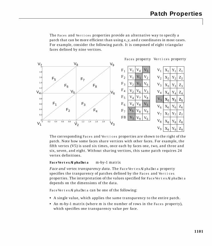
Patch Properties
1101
The Faces and Vertices properties provide an alternative way to specify apatch that can be more efficient than using x, y, and z coordinates in most cases.For example, consider the following patch. It is composed of eight triangularfaces defined by nine vertices.
The corresponding Faces and Vertices properties are shown to the right of thepatch. Note how some faces share vertices with other faces. For example, thefifth vertex (V5) is used six times, once each by faces one, two, and three andsix, seven, and eight. Without sharing vertices, this same patch requires 24vertex definitions.
FaceVertexAlphaData m-by-1 matrix
Face and vertex transparency data. The FaceVertexAlphaData propertyspecifies the tranparency of patches defined by the Faces and Verticesproperties. The interpretation of the values specified for FaceVertexAlphaDatadepends on the dimensions of the data.
FaceVertexAlphaData can be one of the following:
• A single value, which applies the same transparency to the entire patch.
• An m-by-1 matrix (where m is the number of rows in the Faces property),which specifies one transparency value per face.
V1 V4 5
V1 5 V2
V2 5 V6
V2 V6 V3
V4 V7 V8
V4 V8 7
V8 V9
5 V9 V60 0.2 0.4 0.6 0.8 1 1.2 1.4 1.6 1.8 2
0
0.2
0.4
0.6
0.8
1
1.2
1.4
1.6
1.8
2
F1
Faces property
V5
V5
V5
V5
F5 F7
F1 F3
F6 F8
F4F2
F2
F3
F4
F5
F6
F7
F8
V7 V8 V9
V4 V5
V1
V6
V2 V3
V5 X1 Y1 Z1
X2 Y2 Z2
X3 Y3 Z3
X4 Y4 Z4
X5 Y5 Z5
Vertices property
X6 Y6 Z6
X7 Y7 Z7
X8 Y8 Z8
X9 Y9 Z9
X5 Y5 Z5
V1
V2
V3
V4
V5
V6
V7
V8
V9
V5
Patch Properties
1102
• An m-by-1 matrix (where m is the number of rows in the Vertices property),which specifies one transparency value per vertex.
FaceVertexCData matrix
Face and vertex colors. The FaceVertexCData property specifies the color ofpatches defined by the Faces and Vertices properties, and the values are usedwhen FaceColor, EdgeColor, MarkerFaceColor, or MarkerEdgeColor are setappropriately. The interpretation of the values specified for FaceVertexCDatadepends on the dimensions of the data.
For indexed colors, FaceVertexCData can be:
• A single value, which applies a single color to the entire patch
• An n-by-1 matrix, where n is the number of rows in the Faces property,which specifies one color per face
• An n-by-1 matrix, where n is the number of rows in the Vertices property,which specifies one color per vertex
For true colors, FaceVertexCData can be:
• A 1-by-3 matrix , which applies a single color to the entire patch
• An n-by-3 matrix, where n is the number of rows in the Faces property,which specifies one color per face
• An n-by-3 matrix, where n is the number of rows in the Vertices property,which specifies one color per vertex
The following diagram illustrates the various forms of the FaceVertexCDataproperty for a patch having eight faces and nine vertices. The CDataMapping
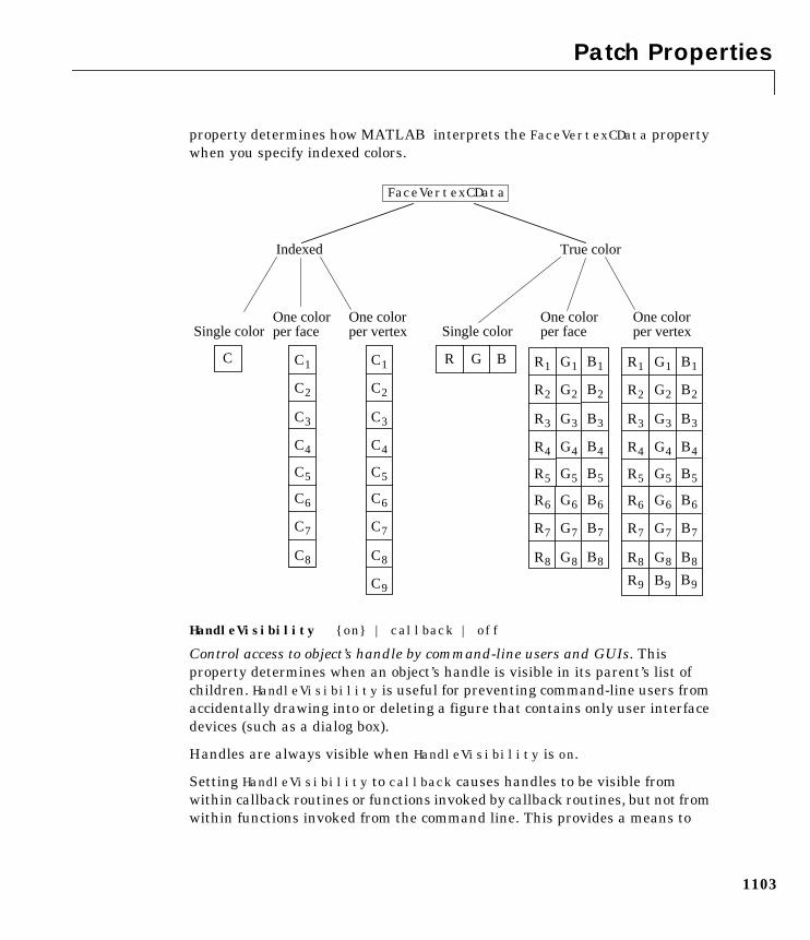
Patch Properties
1103
property determines how MATLAB interprets the FaceVertexCData propertywhen you specify indexed colors.
HandleVisibility on | callback | off
Control access to object’s handle by command-line users and GUIs. Thisproperty determines when an object’s handle is visible in its parent’s list ofchildren. HandleVisibility is useful for preventing command-line users fromaccidentally drawing into or deleting a figure that contains only user interfacedevices (such as a dialog box).
Handles are always visible when HandleVisibility is on.
Setting HandleVisibility to callback causes handles to be visible fromwithin callback routines or functions invoked by callback routines, but not fromwithin functions invoked from the command line. This provides a means to
B9B9
B1
B2
B3
B4
B5
B6
B7
B8
BGC1
C2
C3
C4
C5
C6
C7
C8
C1
C2
C3
C4
C5
C6
C7
C8
C9
C R G1
G2
G3
G4
G5
G6
G7
G8
R1
R2
R3
R4
R5
R6
R7
R8
B1
B2
B3
B4
B5
B6
B7
B8
G1
G2
G3
G4
G5
G6
G7
G8
R1
R2
R3
R4
R5
R6
R7
R8
R9
FaceVertexCData
Indexed
Single colorOne colorper face
One colorper vertex
True color
Single colorOne colorper face
One colorper vertex
Patch Properties
1104
protect GUIs from command-line users, while allowing callback routines tohave complete access to object handles.
Setting HandleVisibility to off makes handles invisible at all times. Thismay be necessary when a callback routine invokes a function that mightpotentially damage the GUI (such as evaluating a user-typed string), and sotemporarily hides its own handles during the execution of that function.
When a handle is not visible in its parent’s list of children, it cannot be returnedby functions that obtain handles by searching the object hierarchy or queryinghandle properties. This includes get, findobj, gca, gcf, gco, newplot, cla, clf,and close.
When a handle’s visibility is restricted using callback or off, the object’shandle does not appear in its parent’s Children property, figures do not appearin the root’s CurrentFigure property, objects do not appear in the root’sCallbackObject property or in the figure’s CurrentObject property, and axesdo not appear in their parent’s Currentaxes property.
You can set the root ShowHiddenHandles property to on to make all handlesvisible, regardless of their HandleVisibility settings (this does not affect thevalues of the HandleVisibility properties).
Handles that are hidden are still valid. If you know an object’s handle, you canset and get its properties, and pass it to any function that operates on handles.
HitTest on | off
Selectable by mouse click. HitTest determines if the patch can become thecurrent object (as returned by the gco command and the figure CurrentObjectproperty) as a result of a mouse click on the patch. If HitTest is off, clickingon the patch selects the object below it (which maybe the axes containing it).
Interruptible on | off
Callback routine interruption mode. The Interruptible property controlswhether a patch callback routine can be interrupted by subsequently invokedcallback routines. Only callback routines defined for the ButtonDownFcn areaffected by the Interruptible property. MATLAB checks for events that caninterrupt a callback routine only when it encounters a drawnow, figure,getframe, or pause command in the routine. See the BusyAction property forrelated information.
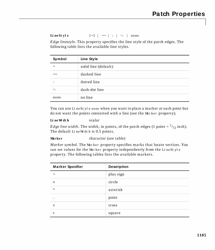
Patch Properties
1105
LineStyle − | −− | : | −. | none
Edge linestyle. This property specifies the line style of the patch edges. Thefollowing table lists the available line styles.
You can use LineStyle none when you want to place a marker at each point butdo not want the points connected with a line (see the Marker property).
LineWidth scalar
Edge line width. The width, in points, of the patch edges (1 point = 1/72 inch).The default LineWidth is 0.5 points.
Marker character (see table)
Marker symbol. The Marker property specifies marks that locate vertices. Youcan set values for the Marker property independently from the LineStyleproperty. The following tables lists the available markers.
Symbol Line Style
− solid line (default)
−− dashed line
: dotted line
−. dash-dot line
none no line
Marker Specifier Description
+ plus sign
o circle
* asterisk
. point
x cross
s square
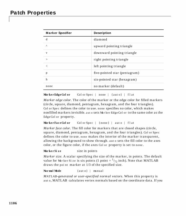
Patch Properties
1106
MarkerEdgeColor ColorSpec | none | auto | flat
Marker edge color. The color of the marker or the edge color for filled markers(circle, square, diamond, pentagram, hexagram, and the four triangles).ColorSpec defines the color to use. none specifies no color, which makesnonfilled markers invisible. auto sets MarkerEdgeColor to the same color as theEdgeColor property.
MarkerFaceColor ColorSpec | none | auto | flat
Marker face color. The fill color for markers that are closed shapes (circle,square, diamond, pentagram, hexagram, and the four triangles). ColorSpecdefines the color to use. none makes the interior of the marker transparent,allowing the background to show through. auto sets the fill color to the axescolor, or the figure color, if the axes Color property is set to none.
MarkerSize size in points
Marker size. A scalar specifying the size of the marker, in points. The defaultvalue for MarkerSize is six points (1 point = 1/72 inch). Note that MATLABdraws the point marker at 1/3 of the specified size.
NormalMode auto | manual
MATLAB-generated or user-specified normal vectors. When this property isauto, MATLAB calculates vertex normals based on the coordinate data. If you
d diamond
^ upward pointing triangle
v downward pointing triangle
> right pointing triangle
< left pointing triangle
p five-pointed star (pentagram)
h six-pointed star (hexagram)
none no marker (default)
Marker Specifier Description
Patch Properties
1107
specify your own vertex normals, MATLAB sets this property to manual anddoes not generate its own data. See also the VertexNormals property.
Parent axes handle
Patch’s parent. The handle of the patch’s parent object. The parent of a patchobject is the axes in which it is displayed. You can move a patch object toanother axes by setting this property to the handle of the new parent.
Selected on | off
Is object selected? When this property is on, MATLAB displays selectionhandles or a dashed box (depending on the number of faces) if theSelectionHighlight property is also on. You can, for example, define theButtonDownFcn to set this property, allowing users to select the object with themouse.
SelectionHighlight on | off
Objects highlight when selected. When the Selected property is on, MATLABindicates the selected state by:
• Drawing handles at each vertex for a single-faced patch.
• Drawing a dashed bounding box for a multi-faced patch.
When SelectionHighlight is off, MATLAB does not draw the handles.
SpecularColorReflectancescalar in the range 0 to 1
Color of specularly reflected light. When this property is 0, the color of thespecularly reflected light depends on both the color of the object from which itreflects and the color of the light source. When set to 1, the color of thespecularly reflected light depends only on the color or the light source (i.e., thelight object Color property). The proportions vary linearly for values inbetween.
SpecularExponent scalar >= 1
Harshness of specular reflection. This property controls the size of the specularspot. Most materials have exponents in the range of 5 to 20.
SpecularStrength scalar >= 0 and <= 1
Intensity of specular light. This property sets the intensity of the specularcomponent of the light falling on the patch. Specular light comes from lightobjects in the axes.
Patch Properties
1108
You can also set the intensity of the ambient and diffuse components of thelight on the patch object. See the AmbientStrength and DiffuseStrengthproperties.
Tag string
User-specified object label. The Tag property provides a means to identifygraphics objects with a user-specified label. This is particularly useful whenconstructing interactive graphics programs that would otherwise need todefine object handles as global variables or pass them as arguments betweencallback routines.
For example, suppose you use patch objects to create borders for a group ofuicontrol objects and want to change the color of the borders in a uicontrol’scallback routine. You can specify a Tag with the patch definition:
patch(X,Y,'k','Tag','PatchBorder')
Then use findobj in the uicontrol’s callback routine to obtain the handle of thepatch and set its FaceColor property.
set(findobj('Tag','PatchBorder'),'FaceColor','w')
Type string (read only)
Class of the graphics object. For patch objects, Type is always the string'patch'.
UIContextMenu handle of a uicontextmenu object
Associate a context menu with the patch. Assign this property the handle of auicontextmenu object created in the same figure as the patch. Use theuicontextmenu function to create the context menu. MATLAB displays thecontext menu whenever you right-click over the patch.
UserData matrix
User-specified data. Any matrix you want to associate with the patch object.MATLAB does not use this data, but you can access it using set and get.
VertexNormals matrix
Surface normal vectors. This property contains the vertex normals for thepatch. MATLAB generates this data to perform lighting calculations. You cansupply your own vertex normal data, even if it does not match the coordinatedata. This can be useful to produce interesting lighting effects.
Patch Properties
1109
Vertices matrix
Vertex coordinates. A matrix containing the x-, y-, z-coordinates for each vertex.See the Faces property for more information.
Visible on | off
Patch object visibility. By default, all patches are visible. When set to off, thepatch is not visible, but still exists and you can query and set its properties.
XData vector or matrix
X-coordinates. The x-coordinates of the points at the vertices of the patch. IfXData is a matrix, each column represents the x-coordinates of a single face ofthe patch. In this case, XData, YData, and ZData must have the samedimensions.
YData vector or matrix
Y-coordinates. The y-coordinates of the points at the vertices of the patch. IfYData is a matrix, each column represents the y-coordinates of a single face ofthe patch. In this case, XData, YData, and ZData must have the samedimensions.
ZData vector or matrix
Z-coordinates. The z-coordinates of the points at the vertices of the patch. IfZData is a matrix, each column represents the z-coordinates of a single face ofthe patch. In this case, XData, YData, and ZData must have the samedimensions.
See Also patch
path
1110
1pathPurpose Control the MATLAB directory search path
GraphicalInterface
As an alternative to the path function, use the Set Path dialog box. To open it,select Set Path from the File menu in the MATLAB desktop.
Syntax pathpath newpathpath(path,'newpath')path('newpath',path)p = path(...)
Description path displays the current MATLAB search path. The initial search path list isdefined by toolbox/local/pathdef.m.
path newpath changes the search path to be comprised of those directoriesnamed in the string, 'newpath'.
path(path,'newpath') appends a new directory to the current search path.
path('newpath',path) prepends a new directory to the current search path.
p = path(...) returns the specified path in string variable p.
Remarks For more information on how MATLAB uses the directory search path, seeHow Functions Work and How MATLAB Determines Which Method to Call.
Note Save any M-files you create and any MATLAB-supplied M-files thatyou edit in a directory that is not in the MATLAB directory tree. If you keep yourfiles in the MATLAB directory tree, they may be overwritten when you install anew version of MATLAB. Also note that locations of files in theMATLAB/toolbox directory tree are loaded and cached in memory at thebeginning of each MATLAB session to improve performance. If you do save anew or edited file in the MATLAB/toolbox directory tree, restart MATLAB oruse the rehash function to reload the directory and update the cache beforeyou use the file.
Examples To add a new directory to the search path on Windows,
path
1111
path(path,’c:tools\goodstuff’)
To add a new directory to the search path on UNIX,
path(path,’/home/tools/goodstuff’)
See Also addpath, genpath, cd, dir, partialpath, rehash, rmpath, what
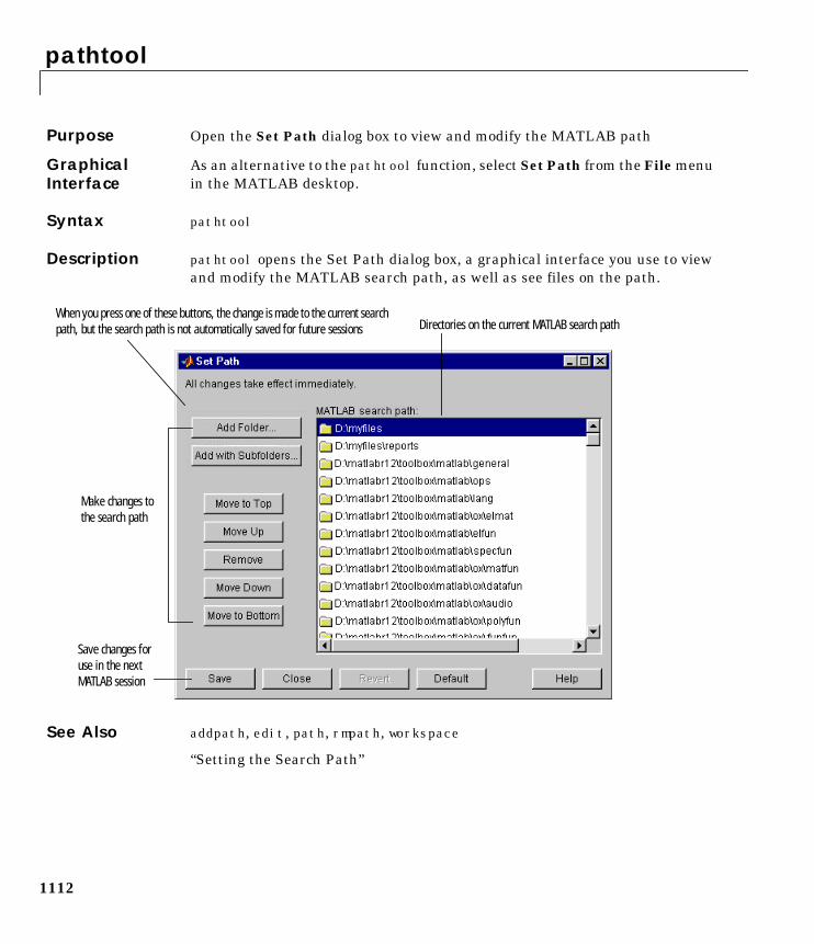
pathtool
1112
1pathtoolPurpose Open the Set Path dialog box to view and modify the MATLAB path
GraphicalInterface
As an alternative to the pathtool function, select Set Path from the File menuin the MATLAB desktop.
Syntax pathtool
Description pathtool opens the Set Path dialog box, a graphical interface you use to viewand modify the MATLAB search path, as well as see files on the path.
See Also addpath, edit, path, rmpath, workspace
“Setting the Search Path”
When you press one of these buttons, the change is made to the current searchpath, but the search path is not automatically saved for future sessions
Make changes tothe search path
Directories on the current MATLAB search path
Save changes foruse in the nextMATLAB session
pause
1113
1pausePurpose Halt execution temporarily
Syntax pausepause(n)pause onpause off
Description pause, by itself, causes M-files to stop and wait for you to press any key beforecontinuing.
pause(n) pauses execution for n seconds before continuing, where n can be anyreal number. The resolution of the clock is platform specific. A fractional pauseof 0.01 seconds should be supported on most platforms.
pause on allows subsequent pause commands to pause execution.
pause off ensures that any subsequent pause or pause(n) statements do notpause execution. This allows normally interactive scripts to run unattended.
See Also drawnow
pbaspect
1114
1pbaspectPurpose Set or query the plot box aspect ratio
Syntax pbaspectpbaspect([aspect_ratio])pbaspect('mode')pbaspect('auto')pbaspect('manual')pbaspect(axes_handle,...)
Description The plot box aspect ratio determines the relative size of the x-, y-, and z-axes.
pbaspect with no arguments returns the plot box aspect ratio of the currentaxes.
pbaspect([aspect_ratio]) sets the plot box aspect ratio in the current axesto the specified value. Specify the aspect ratio as three relative valuesrepresenting the ratio of the x-, y-, and z-axes size. For example, a value of[1 1 1] (the default) means the plot box is a cube (although with stretch-to-fillenabled, it may not appear as a cube). See Remarks.
pbaspect('mode') returns the current value of the plot box aspect ratio mode,which can be either auto (the default) or manual. See Remarks.
pbaspect('auto') sets the plot box aspect ratio mode to auto.
pbaspect('manual') sets the plot box aspect ratio mode to manual.
pbaspect(axes_handle,...) performs the set or query on the axes identifiedby the first argument, axes_handle. If you do not specify an axes handle,pbaspect operates on the current axes.
Remarks pbaspect sets or queries values of the axes object PlotBoxAspectRatio andPlotBoxAspectRatioMode properties.
When the plot box aspect ratio mode is auto, MATLAB sets the ratio to[1 1 1], but may change it to accommodate manual settings of the data aspectratio, camera view angle, or axis limits. See the axes DataAspectRatioproperty for a table listing the interactions between various properties.
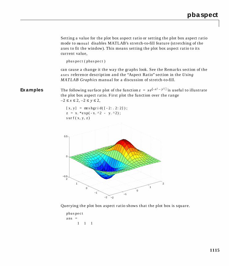
pbaspect
1115
Setting a value for the plot box aspect ratio or setting the plot box aspect ratiomode to manual disables MATLAB’s stretch-to-fill feature (stretching of theaxes to fit the window). This means setting the plot box aspect ratio to itscurrent value,
pbaspect(pbaspect)
can cause a change it the way the graphs look. See the Remarks section of theaxes reference description and the “Aspect Ratio” section in the UsingMATLAB Graphics manual for a discussion of stretch-to-fill.
Examples The following surface plot of the function is useful to illustratethe plot box aspect ratio. First plot the function over the range–2 ≤ x ≤ 2, –2 ≤ y ≤ 2,
[x,y] = meshgrid([-2:.2:2]);z = x.*exp(-x.^2 - y.^2);surf(x,y,z)
Querying the plot box aspect ratio shows that the plot box is square.
pbaspectans =
1 1 1
z xe x2 y2––( )=
−2−1
01
2
−2
−1
0
1
2−0.5
0
0.5
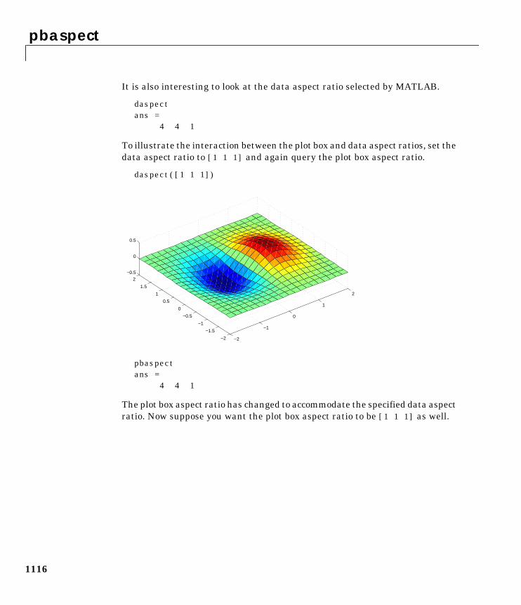
pbaspect
1116
It is also interesting to look at the data aspect ratio selected by MATLAB.
daspectans =
4 4 1
To illustrate the interaction between the plot box and data aspect ratios, set thedata aspect ratio to [1 1 1] and again query the plot box aspect ratio.
daspect([1 1 1])
pbaspectans =
4 4 1
The plot box aspect ratio has changed to accommodate the specified data aspectratio. Now suppose you want the plot box aspect ratio to be [1 1 1] as well.
−2
−1
0
1
2
−2
−1.5
−1
−0.5
0
0.5
1
1.5
2−0.5
0
0.5
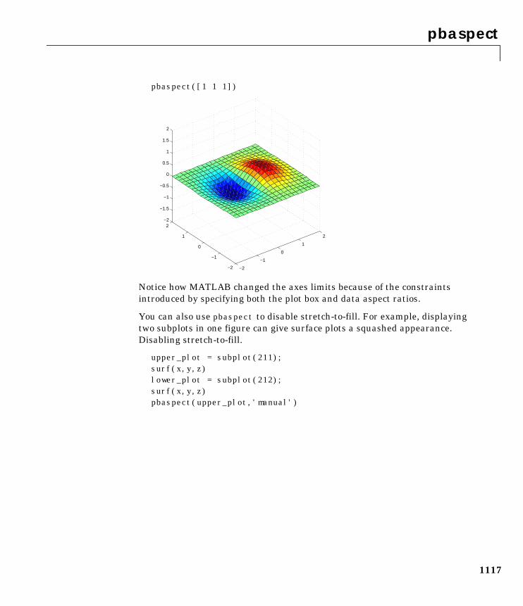
pbaspect
1117
pbaspect([1 1 1])
Notice how MATLAB changed the axes limits because of the constraintsintroduced by specifying both the plot box and data aspect ratios.
You can also use pbaspect to disable stretch-to-fill. For example, displayingtwo subplots in one figure can give surface plots a squashed appearance.Disabling stretch-to-fill.
upper_plot = subplot(211);surf(x,y,z)lower_plot = subplot(212);surf(x,y,z)pbaspect(upper_plot,'manual')
−2
−1
0
1
2
−2
−1
0
1
2−2
−1.5
−1
−0.5
0
0.5
1
1.5
2
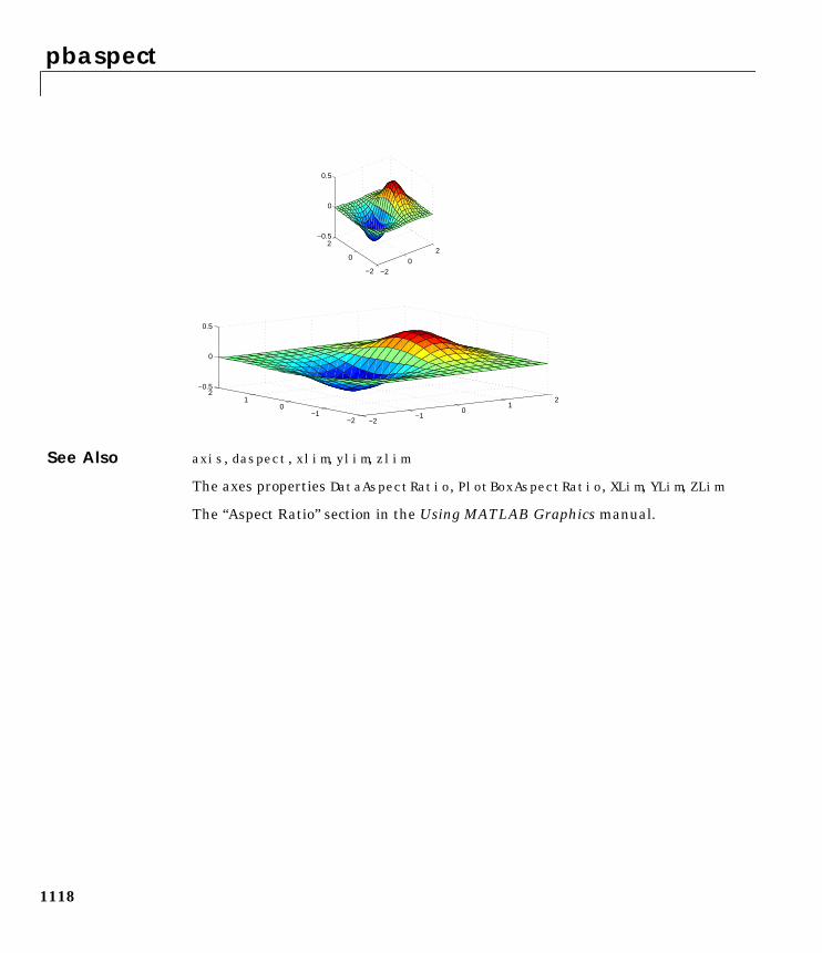
pbaspect
1118
See Also axis, daspect, xlim, ylim, zlim
The axes properties DataAspectRatio, PlotBoxAspectRatio, XLim, YLim, ZLim
The “Aspect Ratio” section in the Using MATLAB Graphics manual.
−20
2
−2
0
2−0.5
0
0.5
−2−1
01
2
−2−1
01
2−0.5
0
0.5
pcg
1119
1pcgPurpose Preconditioned Conjugate Gradients method
Syntax x = pcg(A,b)pcg(A,b,tol)pcg(A,b,tol,maxit)pcg(A,b,tol,maxit,M)pcg(A,b,tol,maxit,M1,M2)pcg(A,b,tol,maxit,M1,M2,x0)pcg(A,b,tol,maxit,M1,M2,x0,p1,p2,...)[x,flag] = pcg(A,b,tol,maxit,M1,M2,x0,p1,p2,...)[x,flag,relres] = pcg(A,b,tol,maxit,M1,M2,x0,p1,p2,...)[x,flag,relres,iter] = pcg(A,b,tol,maxit,M1,M2,x0,p1,p2,...)[x,flag,relres,iter,resvec] = pcg(A,b,tol,maxit,M1,M2,x0,p1,p2,...)
Description x = pcg(A,b) attempts to solve the system of linear equations A*x=b for x.The n-by-n coefficient matrix Amust be symmetric and positive definite and thecolumn vector b must have length n. A can be a function afun such that afun(x)returns A*x.
If pcg converges, a message to that effect is displayed. If pcg fails to convergeafter the maximum number of iterations or halts for any reason, a warningmessage is printed displaying the relative residual norm(b-A*x)/norm(b) andthe iteration number at which the method stopped or failed.
pcg(A,b,tol) specifies the tolerance of the method. If tol is [], then pcg usesthe default, 1e-6.
pcg(A,b,tol,maxit) specifies the maximum number of iterations. If maxit is[], then pcg uses the default, min(n,20).
pcg(A,b,tol,maxit,M) and pcg(A,b,tol,maxit,M1,M2) use symmetricpositive definite preconditioner M or M = M1*M2 and effectively solve the systeminv(M)*A*x = inv(M)*b for x. If M is [] then pcg applies no preconditioner. Mcan be a function that returns M\x.
pcg(A,b,tol,maxit,M1,M2,x0) specifies the initial guess. If x0 is [], then pcguses the default, an all-zero vector.
pcg
1120
pcg(afun,b,tol,maxit,m1fun,m2fun,x0,p1,p2,...) passes parametersp1,p2,... to functions afun(x,p1,p2,...), m1fun(x,p1,p2,...), andm2fun(x,p1,p2,...).
[x,flag] = pcg(A,b,tol,maxit,M1,M2,x0) also returns a convergence flag.
Whenever flag is not 0, the solution x returned is that with minimal normresidual computed over all the iterations. No messages are displayed if theflag output is specified.
[x,flag,relres] = pcg(A,b,tol,maxit,M1,M2,x0) also returns the relativeresidual norm(b-A*x)/norm(b). If flag is 0, relres <= tol.
[x,flag,relres,iter] = pcg(A,b,tol,maxit,M1,M2,x0) also returns theiteration number at which x was computed, where 0 <= iter <= maxit.
[x,flag,relres,iter,resvec] = pcg(A,b,tol,maxit,M1,M2,x0) alsoreturns a vector of the residual norms at each iteration includingnorm(b-A*x0).
Examples Example 1.
A = gallery('wilk',21);b = sum(A,2);tol = 1e-12;maxit = 15;M = diag([10:-1:1 1 1:10]);
Flag Convergence
0 pcg converged to the desired tolerance tol within maxititerations.
1 pcg iterated maxit times but did not converge.
2 Preconditioner M was ill-conditioned.
3 pcg stagnated. (Two consecutive iterates were the same.)
4 One of the scalar quantities calculated during pcg becametoo small or too large to continue computing.
pcg
1121
[x,flag,rr,iter,rv] = pcg(A,b,tol,maxit,M);
Alternatively, use this one-line matrix-vector product function
function y = afun(x,n)y = [0; x(1:n-1)] + [((n-1)/2:-1:0)'; (1:(n-1)/2)'].*x + [x(2:n); 0];
and this one-line preconditioner backsolve function
function y = mfun(r,n)y = r ./ [((n-1)/2:-1:1)'; 1; (1:(n-1)/2)'];
as inputs to pcg
[x1,flag1,rr1,iter1,rv1] = pcg(@afun,b,tol,maxit,@mfun,... [],[],21);
Example 2.
A = delsq(numgrid('C',25));b = ones(length(A),1);[x,flag] = pcg(A,b)
flag is 1 because pcg does not converge to the default tolerance of 1e-6 withinthe default 20 iterations.
R = cholinc(A,1e-3);[x2,flag2,relres2,iter2,resvec2] = pcg(A,b,1e-8,10,R',R)
flag2 is 0 because pcg converges to the tolerance of 1.2e-9 (the value ofrelres2) at the sixth iteration (the value of iter2) when preconditioned by theincomplete Cholesky factorization with a drop tolerance of 1e-3.resvec2(1) = norm(b) and resvec2(7) = norm(b-A*x2). You can follow theprogress of pcg by plotting the relative residuals at each iteration starting fromthe initial estimate (iterate number 0).
semilogy(0:iter2,resvec2/norm(b),'-o')xlabel('iteration number')ylabel('relative residual')
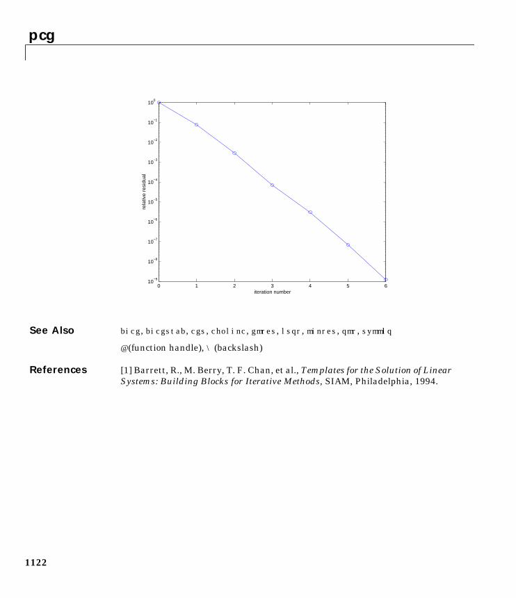
pcg
1122
See Also bicg, bicgstab, cgs, cholinc, gmres, lsqr, minres, qmr, symmlq
@ (function handle), \ (backslash)
References [1] Barrett, R., M. Berry, T. F. Chan, et al., Templates for the Solution of LinearSystems: Building Blocks for Iterative Methods, SIAM, Philadelphia, 1994.
0 1 2 3 4 5 610
−9
10−8
10−7
10−6
10−5
10−4
10−3
10−2
10−1
100
iteration number
rela
tive
resi
dual
pchip
1123
1pchipPurpose Piecewise Cubic Hermite Interpolating Polynomial (PCHIP)
Syntax yi = pchip(x,y,xi)pp = pchip(x,y)
Description yi = pchip(x,y,xi) returns vector yi containing elements corresponding tothe elements of xi and determined by piecewise cubic interpolation withinvectors x and y. The vector x specifies the points at which the data y is given.If y is a matrix, then the interpolation is performed for each column of y andyi is length(xi)-by-size(y,2).
pp = pchip(x,y) returns a piecewise polynomial structure for use by ppval.x can be a row or column vector. y is a row or column vector of the same lengthas x, or a matrix with length(x) columns.
pchip finds values of an underlying interpolating function atintermediate points. satisfies:
• is a different cubic on each subinterval, .
• interpolates the data, i.e. .
• The first derivative, , is continuous.
• The second derivative, , is piecewise linear.
• is probably not continuous; there may be jumps at .
• preserves both the shape of the data and monotonicity.
• On intervals where the data is monotonic, so is .
• At points where the data has a local extremum, so does .
Note If is a matrix, satisfies the above for each column of .
Comparing pchip with spline:
• spline is smoother, i.e. is continuous.
• spline is more accurate if the data are values of a smooth function.
• pchip has no overshoots and less oscillation if the data are not smooth.
P x( )P x( )
P x( ) xk x xk 1+≤ ≤P x( ) P xk( ) yk=
P′ x( )P″ x( )
P″ x( ) xk
P x( )P x( )
P x( )
y P x( ) y
S″ x( )
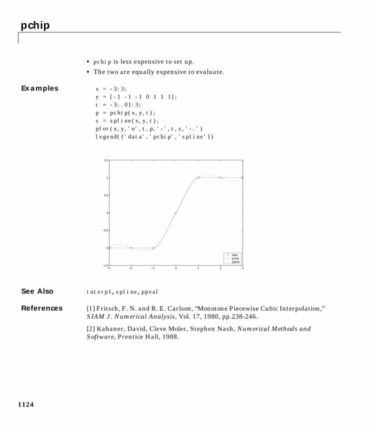
pchip
1124
• pchip is less expensive to set up.
• The two are equally expensive to evaluate.
Examples x = -3:3;y = [-1 -1 -1 0 1 1 1];t = -3:.01:3;p = pchip(x,y,t);s = spline(x,y,t);plot(x,y,'o',t,p,'-',t,s,'-.')legend('data','pchip','spline')
See Also interp1, spline, ppval
References [1] Fritsch, F. N. and R. E. Carlson, “Monotone Piecewise Cubic Interpolation,”SIAM J. Numerical Analysis, Vol. 17, 1980, pp.238-246.
[2] Kahaner, David, Cleve Moler, Stephen Nash, Numerical Methods andSoftware, Prentice Hall, 1988.
−3 −2 −1 0 1 2 3−1.5
−1
−0.5
0
0.5
1
1.5
datapchipspline
pcode
1125
1pcodePurpose Create preparsed pseudocode file (P-file)
Syntax pcode funpcode *.mpcode fun1 fun2 ...pcode... -inplace
Description pcode fun parses the M-file fun.m into the P-file fun.p and puts it into thecurrent directory. The original M-file can be anywhere on the search path.
pcode *.m creates P-files for all the M-files in the current directory.
pcode fun1 fun2 ... creates P-files for the listed functions.
pcode... -inplace creates P-files in the same directory as the M-files. Anerror occurs if the files can’t be created.
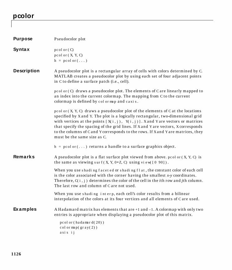
pcolor
1126
1pcolorPurpose Pseudocolor plot
Syntax pcolor(C)pcolor(X,Y,C)h = pcolor(...)
Description A pseudocolor plot is a rectangular array of cells with colors determined by C.MATLAB creates a pseudocolor plot by using each set of four adjacent pointsin C to define a surface patch (i.e., cell).
pcolor(C) draws a pseudocolor plot. The elements of C are linearly mapped toan index into the current colormap. The mapping from C to the currentcolormap is defined by colormap and caxis.
pcolor(X,Y,C) draws a pseudocolor plot of the elements of C at the locationsspecified by X and Y. The plot is a logically rectangular, two-dimensional gridwith vertices at the points [X(i,j), Y(i,j)]. X and Y are vectors or matricesthat specify the spacing of the grid lines. If X and Y are vectors, X correspondsto the columns of C and Y corresponds to the rows. If X and Y are matrices, theymust be the same size as C.
h = pcolor(...) returns a handle to a surface graphics object.
Remarks A pseudocolor plot is a flat surface plot viewed from above. pcolor(X,Y,C) isthe same as viewing surf(X,Y,0*Z,C) using view([0 90]).
When you use shading faceted or shading flat, the constant color of each cellis the color associated with the corner having the smallest x-y coordinates.Therefore, C(i,j) determines the color of the cell in the ith row and jth column.The last row and column of C are not used.
When you use shading interp, each cell’s color results from a bilinearinterpolation of the colors at its four vertices and all elements of C are used.
Examples A Hadamard matrix has elements that are +1 and –1. A colormap with only twoentries is appropriate when displaying a pseudocolor plot of this matrix.
pcolor(hadamard(20))colormap(gray(2))axis ij
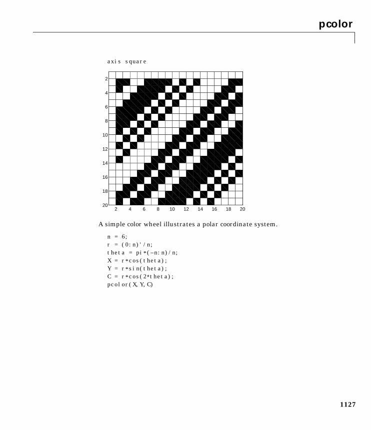
pcolor
1127
axis square
A simple color wheel illustrates a polar coordinate system.
n = 6;r = (0:n)'/n;theta = pi*(–n:n)/n;X = r*cos(theta);Y = r*sin(theta);C = r*cos(2∗theta);pcolor(X,Y,C)
2 4 6 8 10 12 14 16 18 20
2
4
6
8
10
12
14
16
18
20
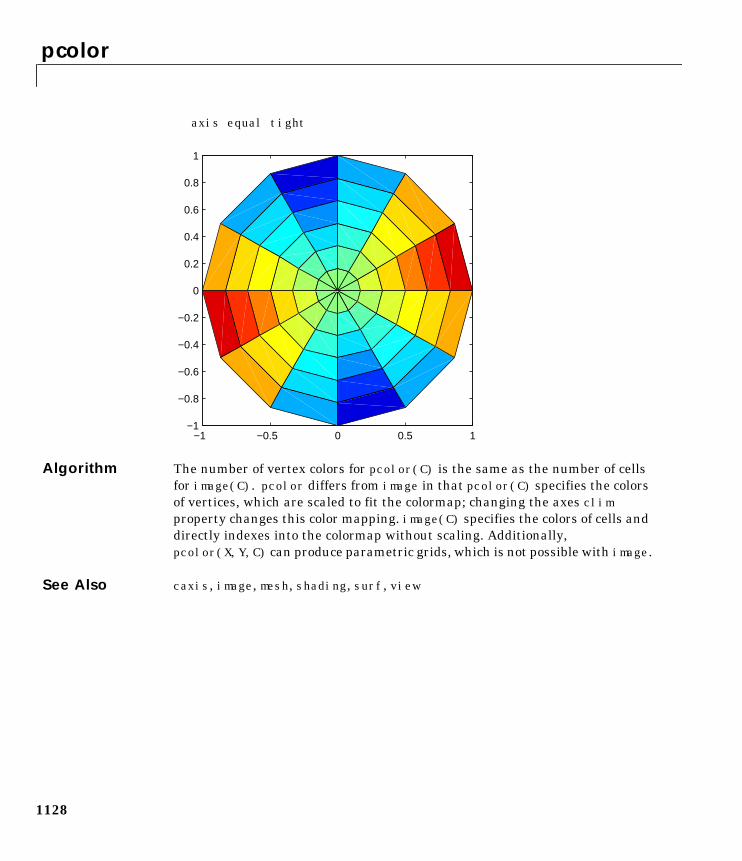
pcolor
1128
axis equal tight
Algorithm The number of vertex colors for pcolor(C) is the same as the number of cellsfor image(C). pcolor differs from image in that pcolor(C) specifies the colorsof vertices, which are scaled to fit the colormap; changing the axes climproperty changes this color mapping. image(C) specifies the colors of cells anddirectly indexes into the colormap without scaling. Additionally,pcolor(X,Y,C) can produce parametric grids, which is not possible with image.
See Also caxis, image, mesh, shading, surf, view
−1 −0.5 0 0.5 1−1
−0.8
−0.6
−0.4
−0.2
0
0.2
0.4
0.6
0.8
1
pdepe
1129
1pdepePurpose Solve initial-boundary value problems for systems of parabolic and ellipticpartial differential equations (PDEs) in one space variable and time
Syntax sol = pdepe(m,pdefun,icfun,bcfun,xmesh,tspan)sol = pdepe(m,pdefun,icfun,bcfun,xmesh,tspan,options)sol = pdepe(m,pdefun,icfun,bcfun,xmesh,tspan,options,p1,p2...)
Arguments
Description sol = pdepe(m,pdefun,icfun,bcfun,xmesh,tspan) solves initial-boundaryvalue problems for systems of parabolic and elliptic PDEs in the one spacevariable and time . The ordinary differential equations (ODEs) resultingfrom discretization in space are integrated to obtain approximate solutions attimes specified in tspan. The pdepe function returns values of the solution ona mesh provided in xmesh.
m A parameter corresponding to the symmetry of the problem. m canbe slab = 0, cylindrical = 1, or spherical = 2.
pdefun A function that defines the components of the PDE.
icfun A function that defines the initial conditions.
bcfun A function that defines the boundary conditions.
xmesh A vector [x0, x1, ..., xn] specifying the points at which a numericalsolution is requested for every value in tspan. The elements ofxmesh must satisfy x0 < x1 < ... < xn. The length of xmesh mustbe ≥ 3.
tspan A vector [t0, t1, ..., tf] specifying the points at which a solution isrequested for every value in xmesh. The elements of tspan mustsatisfy t0 < t1 < ... < tf. The length of tspan must be ≥ 3.
options Some options of the underlying ODE solver are available in pdepe:RelTol, AbsTol, NormControl, InitialStep, and MaxStep. In mostcases, default values for these options provide satisfactorysolutions. See odeset for details.
p1,p2,... Optional parameters to be passed to pdefun, icfun, and bcfun.
x t
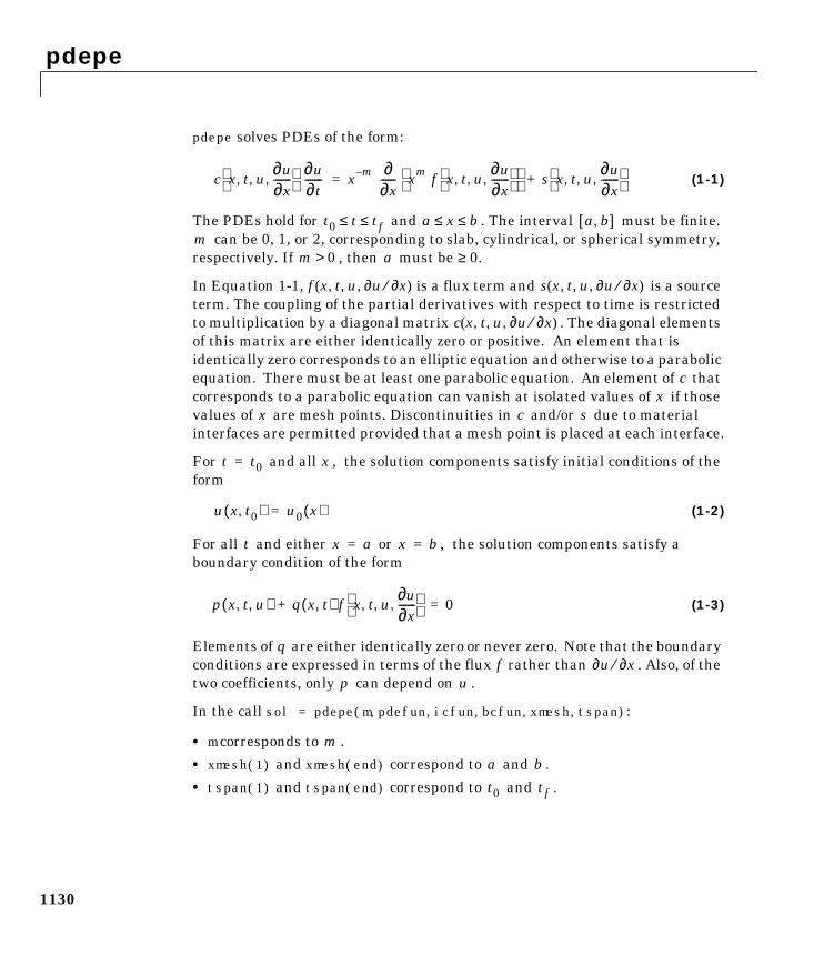
pdepe
1130
pdepe solves PDEs of the form:
(1-1)
The PDEs hold for and . The interval must be finite.can be 0, 1, or 2, corresponding to slab, cylindrical, or spherical symmetry,
respectively. If , then must be ≥ 0.
In Equation 1-1, is a flux term and is a sourceterm. The coupling of the partial derivatives with respect to time is restrictedto multiplication by a diagonal matrix . The diagonal elementsof this matrix are either identically zero or positive. An element that isidentically zero corresponds to an elliptic equation and otherwise to a parabolicequation. There must be at least one parabolic equation. An element of thatcorresponds to a parabolic equation can vanish at isolated values of if thosevalues of are mesh points. Discontinuities in and/or due to materialinterfaces are permitted provided that a mesh point is placed at each interface.
For and all , the solution components satisfy initial conditions of theform
(1-2)
For all and either or , the solution components satisfy aboundary condition of the form
(1-3)
Elements of are either identically zero or never zero. Note that the boundaryconditions are expressed in terms of the flux rather than . Also, of thetwo coefficients, only can depend on .
In the call sol = pdepe(m,pdefun,icfun,bcfun,xmesh,tspan):
• m corresponds to .
• xmesh(1) and xmesh(end) correspond to and .
• tspan(1) and tspan(end) correspond to and .
c x t u∂u∂x-------, , ,
∂u∂t------- x m– ∂
∂x------ xm f x t u
∂u∂x-------, , ,
s x t u
∂u∂x-------, , ,
+=
t0 t t f≤ ≤ a x b≤ ≤ a b,[ ]m
m 0> a
f x t u ∂u ∂x⁄, , ,( ) s x t u ∂u ∂x⁄, , ,( )
c x t u ∂u ∂x⁄, , ,( )
cx
x c s
t t0= x
u x t0,( ) u0 x( )=
t x a= x b=
p x t u, ,( ) q x t,( ) f x t uu∂x∂
-------, , , + 0=
qf ∂u ∂x⁄
p u
m
a b
t0 tf
pdepe
1131
• pdefun computes the terms , , and (Equation 1-1). It has the form[c,f,s] = pdefun(x,t,u,dudx)
The input arguments are scalars x and t and vectors u and dudx thatapproximate the solution and its partial derivative with respect to ,respectively. c, f, and s are column vectors. c stores the diagonal elements ofthe matrix (Equation 1-1).
• icfun evaluates the initial conditions. It has the formu = icfun(x)
When called with an argument x, icfun evaluates and returns the initialvalues of the solution components at x in the column vector u.
• bcfun evaluates the terms and of the boundary conditions(Equation 1-3). It has the form[pl,ql,pr,qr] = bcfun(xl,ul,xr,ur,t)
ul is the approximate solution at the left boundary xl = and ur is theapproximate solution at the right boundary xr = . pl and ql are columnvectors corresponding to and evaluated at xl, similarly pr and qrcorrespond to xr. When and , boundedness of the solution near
requires that the flux vanish at . pdepe imposes this boundarycondition automatically and it ignores values returned in pl and ql.
pdepe returns the solution as a multidimensional array sol.= ui = sol(:,:,i) is an approximation to the ith component of the solution
vector . The element ui(j,k) = sol(j,k,i) approximates at= (tspan(j),xmesh(k)).
ui = sol(j,:,i) approximates component i of the solution at time tspan(j) andmesh points xmesh(:). Use pdeval to compute the approximation and itspartial derivative at points not included in xmesh. See pdeval fordetails.
sol = pdepe(m,pdefun,icfun,bcfun,xmesh,tspan,options) solves as abovewith default integration parameters replaced by values in options, anargument created with the odeset function. Only some of the options of theunderlying ODE solver are available in pdepe: RelTol, AbsTol, NormControl,InitialStep, and MaxStep. The defaults obtained by leaving off the inputargument options will generally be satisfactory. See odeset for details.
c f s
u x
c
p q
ab
p qm 0> a 0=
x 0= f xa 0=
uiu ui
t x,( )
∂ui ∂x⁄
pdepe
1132
sol = pdepe(m,pdefun,icfun,bcfun,xmesh,tspan,options,p1,p2...)passes the additional parameters p1, p2, ... to the functions pdefun, icfun, andbcfun. Use options = [] as a placeholder if no options are set.
Remarks • The arrays xmesh and tspan play different roles in pdepe.
tspan – The pdepe function performs the time integration with an ODEsolver that selects both the time step and formula dynamically. Theelements of tspan merely specify where you want answers and the costdepends weakly on the length of tspan.
xmesh – Second order approximations to the solution are made on the meshspecified in xmesh. Generally, it is best to use closely spaced mesh pointswhere the solution changes rapidly. pdepe does not select the mesh inautomatically. You must provide an appropriate fixed mesh in xmesh. Thecost depends strongly on the length of xmesh. When , it is not necessaryto use a fine mesh near to account for the coordinate singularity.
• The time integration is done with ode15s. pdepe exploits the capabilities ofode15s for solving the differential-algebraic equations that arise whenEquation 1-1 contains elliptic equations, and for handling Jacobians with aspecified sparsity pattern.
• After discretization, elliptic equations give rise to algebraic equations. If theelements of the initial conditions vector that correspond to elliptic equationsare not “consistent” with the discretization, pdepe tries to adjust them beforebeginning the time integration. For this reason, the solution returned for theinitial time may have a discretization error comparable to that at any othertime. If the mesh is sufficiently fine, pdepe can find consistent initialconditions close to the given ones. If pdepe displays a message that it hasdifficulty finding consistent initial conditions, try refining the mesh.
No adjustment is necessary for elements of the initial conditions vector thatcorrespond to parabolic equations.
x
m 0>x 0=
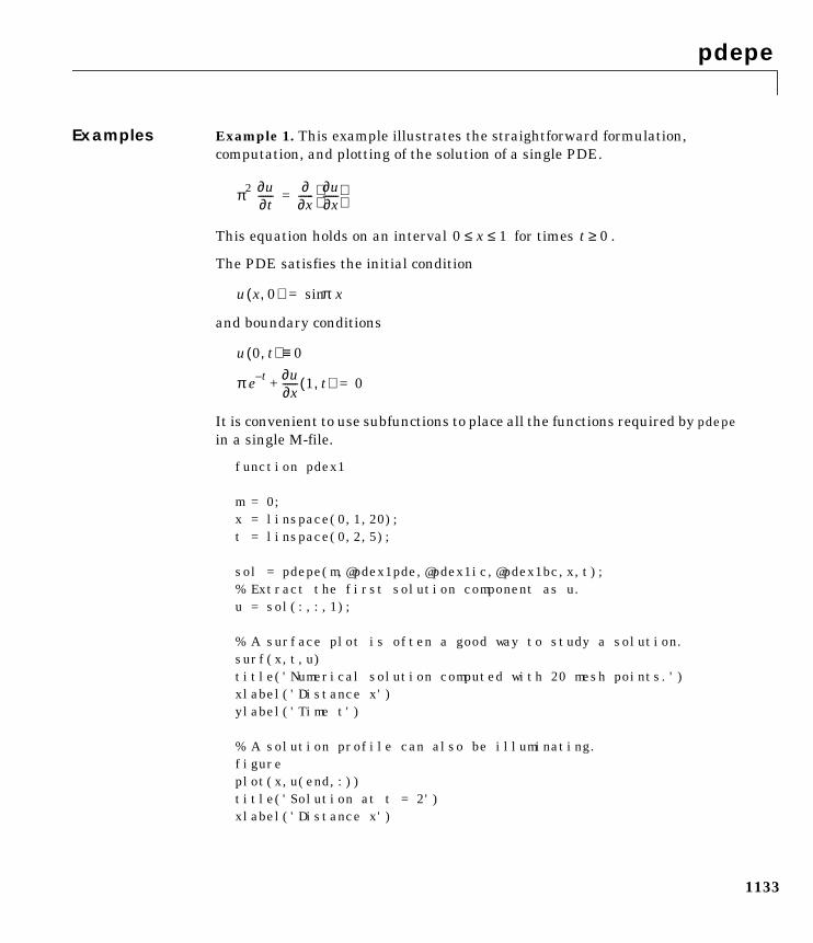
pdepe
1133
Examples Example 1. This example illustrates the straightforward formulation,computation, and plotting of the solution of a single PDE.
This equation holds on an interval for times .
The PDE satisfies the initial condition
and boundary conditions
It is convenient to use subfunctions to place all the functions required by pdepein a single M-file.
function pdex1
m = 0;x = linspace(0,1,20);t = linspace(0,2,5);
sol = pdepe(m,@pdex1pde,@pdex1ic,@pdex1bc,x,t);% Extract the first solution component as u.u = sol(:,:,1);
% A surface plot is often a good way to study a solution.surf(x,t,u)title('Numerical solution computed with 20 mesh points.')xlabel('Distance x')ylabel('Time t')
% A solution profile can also be illuminating.figureplot(x,u(end,:))title('Solution at t = 2')xlabel('Distance x')
π2 ∂u∂t------ ∂
∂x------ ∂u
∂x------
=
0 x 1≤ ≤ t 0≥
u x 0,( ) πxsin=
u 0 t,( ) 0≡
π e t– ∂u∂x------ 1 t,( )+ 0=
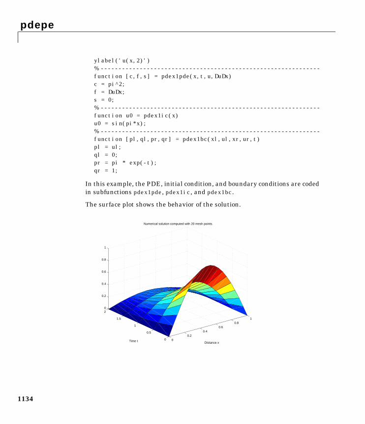
pdepe
1134
ylabel('u(x,2)')% --------------------------------------------------------------function [c,f,s] = pdex1pde(x,t,u,DuDx)c = pi^2;f = DuDx;s = 0;% --------------------------------------------------------------function u0 = pdex1ic(x)u0 = sin(pi*x);% --------------------------------------------------------------function [pl,ql,pr,qr] = pdex1bc(xl,ul,xr,ur,t)pl = ul;ql = 0;pr = pi * exp(-t);qr = 1;
In this example, the PDE, initial condition, and boundary conditions are codedin subfunctions pdex1pde, pdex1ic, and pdex1bc.
The surface plot shows the behavior of the solution.
00.2
0.40.6
0.81
0
0.5
1
1.5
20
0.2
0.4
0.6
0.8
1
Distance x
Numerical solution computed with 20 mesh points.
Time t
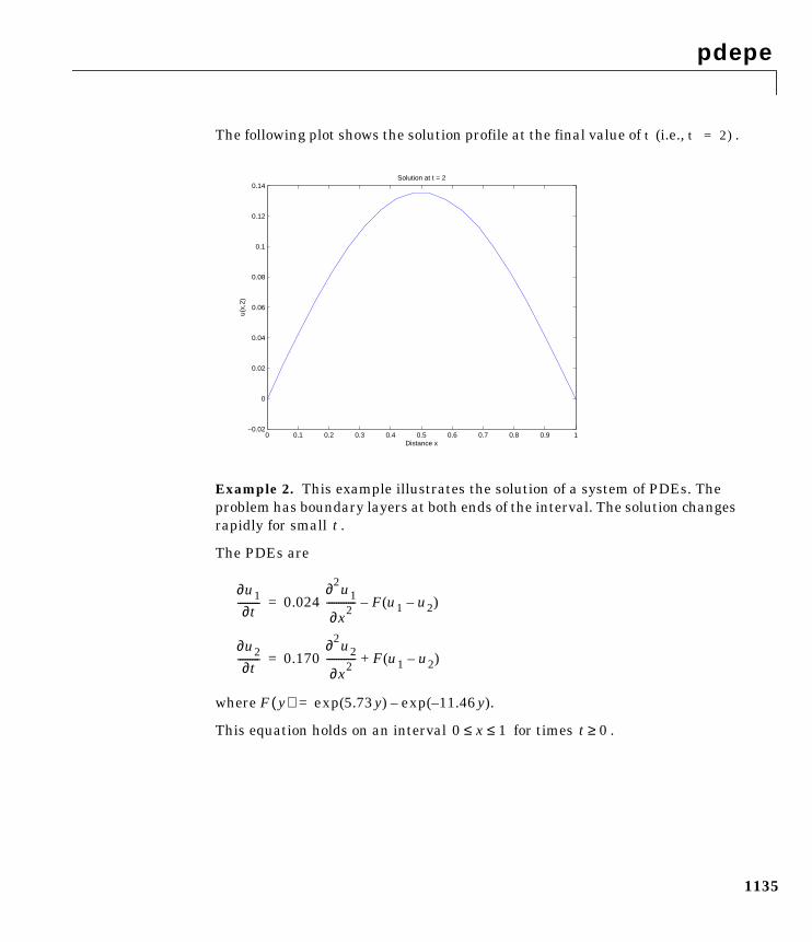
pdepe
1135
The following plot shows the solution profile at the final value of t (i.e., t = 2).
Example 2. This example illustrates the solution of a system of PDEs. Theproblem has boundary layers at both ends of the interval. The solution changesrapidly for small .
The PDEs are
where .
This equation holds on an interval for times .
0 0.1 0.2 0.3 0.4 0.5 0.6 0.7 0.8 0.9 1−0.02
0
0.02
0.04
0.06
0.08
0.1
0.12
0.14Solution at t = 2
Distance x
u(x,
2)
t
∂u1∂t
--------- 0.024∂2u1
∂x2------------ F u1 u2–( )–=
∂u2∂t
--------- 0.170∂2u2
∂x2------------ F u1 u2–( )+=
F y( ) exp 5.73 y( ) exp 11.46– y( )–=
0 x 1≤ ≤ t 0≥
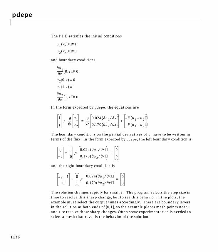
pdepe
1136
The PDE satisfies the initial conditions
and boundary conditions
In the form expected by pdepe, the equations are
The boundary conditions on the partial derivatives of have to be written interms of the flux. In the form expected by pdepe, the left boundary condition is
and the right boundary condition is
The solution changes rapidly for small . The program selects the step size intime to resolve this sharp change, but to see this behavior in the plots, theexample must select the output times accordingly. There are boundary layersin the solution at both ends of [0,1], so the example places mesh points near 0and 1 to resolve these sharp changes. Often some experimentation is needed toselect a mesh that reveals the behavior of the solution.
u1 x 0,( ) 1≡
u2 x 0,( ) 0≡
∂u1∂x
--------- 0 t,( ) 0≡
u2 0 t,( ) 0≡
u1 1 t,( ) 1≡
∂u2∂x
--------- 1 t,( ) 0≡
1
1
∂∂t-----
u1
u2
∂∂x------
0.024 ∂u1 ∂x⁄( )
0.170 ∂u2 ∂x⁄( )
F u1 u2–( )–
F u1 u2–( )+=.∗
u
0u2
1
0+
0.024 ∂u1 ∂x⁄( )
0.170 ∂u2 ∂x⁄( )
0
0=.∗
u1 1–
0
0
1+
0.024 ∂u1 ∂x⁄( )
0.170 ∂u2 ∂x⁄( )0
0=.∗
t
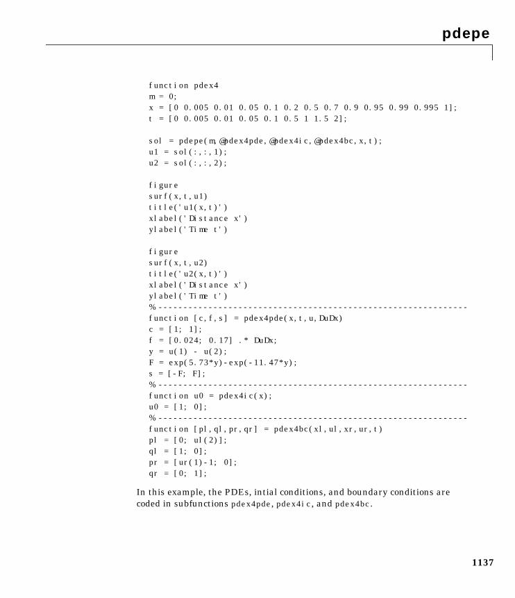
pdepe
1137
function pdex4m = 0;x = [0 0.005 0.01 0.05 0.1 0.2 0.5 0.7 0.9 0.95 0.99 0.995 1];t = [0 0.005 0.01 0.05 0.1 0.5 1 1.5 2];
sol = pdepe(m,@pdex4pde,@pdex4ic,@pdex4bc,x,t);u1 = sol(:,:,1);u2 = sol(:,:,2);
figuresurf(x,t,u1)title('u1(x,t)')xlabel('Distance x')ylabel('Time t')
figuresurf(x,t,u2)title('u2(x,t)')xlabel('Distance x')ylabel('Time t')% --------------------------------------------------------------function [c,f,s] = pdex4pde(x,t,u,DuDx)c = [1; 1];f = [0.024; 0.17] .* DuDx;y = u(1) - u(2);F = exp(5.73*y)-exp(-11.47*y);s = [-F; F];% --------------------------------------------------------------function u0 = pdex4ic(x);u0 = [1; 0];% --------------------------------------------------------------function [pl,ql,pr,qr] = pdex4bc(xl,ul,xr,ur,t)pl = [0; ul(2)];ql = [1; 0];pr = [ur(1)-1; 0];qr = [0; 1];
In this example, the PDEs, intial conditions, and boundary conditions arecoded in subfunctions pdex4pde, pdex4ic, and pdex4bc.
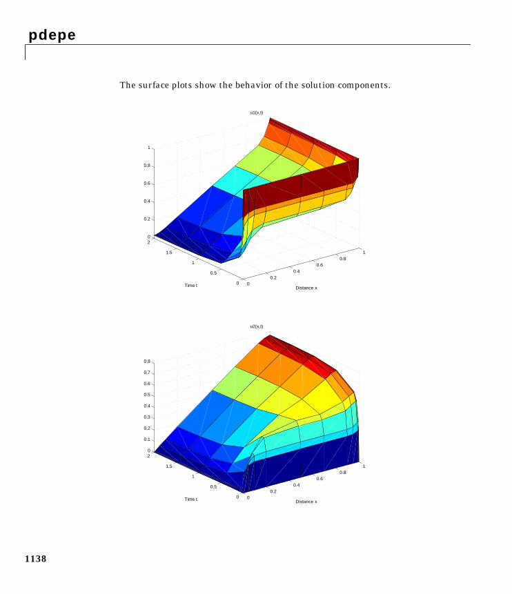
pdepe
1138
The surface plots show the behavior of the solution components.
00.2
0.40.6
0.81
0
0.5
1
1.5
20
0.2
0.4
0.6
0.8
1
Distance x
u1(x,t)
Time t
00.2
0.40.6
0.81
0
0.5
1
1.5
20
0.1
0.2
0.3
0.4
0.5
0.6
0.7
0.8
Distance x
u2(x,t)
Time t
pdepe
1139
See Also function_handle, pdeval, ode15s, odeset, odeget
References [1] Skeel, R. D. and M. Berzins, “A Method for the Spatial Discretization ofParabolic Equations in One Space Variable,” SIAM Journal on Scientific andStatistical Computing, Vol. 11, 1990, pp.1-32.
pdeval
1140
1pdevalPurpose Evaluate the numerical solution of a PDE using the output of pdepe
Syntax [uout,duoutdx] = pdeval(m,xmesh,ui,xout)
Arguments
Description [uout,duoutdx] = pdeval(m,x,ui,xout) approximates the solution andits partial derivative at points from the interval [x0,xn]. The pdevalfunction returns the computed values in uout and duoutdx, respectively.
Note pdeval evaluates the partial derivative rather than the flux .Although the flux is continuous, the partial derivative may have a jump at amaterial interface.
See Also pdepe
m Symmetry of the problem: slab = 0, cylindrical = 1, spherical = 2.This is the first input argument used in the call to pdepe.
xmesh A vector [x0, x1, ..., xn] specifying the points at which the elementsof ui were computed. This is the same vector with which pdepe wascalled.
ui A vector sol(j,:,i) that approximates component i of the solution attime and mesh points xmesh, where sol is the solution returnedby pdepe.
xout A vector of points from the interval [x0,xn] at which the interpolatedsolution is requested.
tf
ui∂ui ∂x⁄
∂ui ∂x⁄ f
peaks
1141
1peaksPurpose A sample function of two variables.
Syntax Z = peaks;Z = peaks(n);Z = peaks(V);Z = peaks(X,Y);
peaks;peaks(N);peaks(V);peaks(X,Y);
[X,Y,Z] = peaks;[X,Y,Z] = peaks(n);[X,Y,Z] = peaks(V);
Description peaks is a function of two variables, obtained by translating and scalingGaussian distributions, which is useful for demonstrating mesh, surf, pcolor,contour, and so on.
Z = peaks; returns a 49-by-49 matrix.
Z = peaks(n); returns an n-by-n matrix.
Z = peaks(V); returns an n-by-n matrix, where n = length(V).
Z = peaks(X,Y); evaluates peaks at the given X and Y (which must be the samesize) and returns a matrix the same size.
peaks(...) (with no output argument) plots the peaks function with surf.
[X,Y,Z] = peaks(...); returns two additional matrices, X and Y, forparametric plots, for example, surf(X,Y,Z,del2(Z)). If not given as input, theunderlying matrices X and Y are:
[X,Y] = meshgrid(V,V)
where V is a given vector, or V is a vector of length n with elements equallyspaced from −3 to 3. If no input argument is given, the default n is 49.
See Also meshgrid, surf
perms
1142
1permsPurpose All possible permutations
Syntax P = perms(v)
Description P = perms(v), where v is a row vector of length n, creates a matrix whose rowsconsist of all possible permutations of the n elements of v. Matrix P contains n!rows and n columns.
Examples The command perms(2:2:6) returns all the permutations of the numbers 2, 4,and 6:
2 4 62 6 44 2 64 6 26 4 26 2 4
Limitations This function is only practical for situations where n is less than about 15.
See Also nchoosek, permute, randperm
permute
1143
1permutePurpose Rearrange the dimensions of a multidimensional array
Syntax B = permute(A,order)
Description B = permute(A,order) rearranges the dimensions of A so that they are in theorder specified by the vector order. B has the same values of A but the order ofthe subscripts needed to access any particular element is rearranged asspecified by order. All the elements of order must be unique.
Remarks permute and ipermute are a generalization of transpose (.') formultidimensional arrays.
Examples Given any matrix A, the statement
permute(A,[2 1])
is the same as A'.
For example:
A = [1 2; 3 4]; permute(A,[2 1])ans = 1 3 2 4
The following code permutes a three-dimensional array:
X = rand(12,13,14);Y = permute(X,[2 3 1]);size(Y)ans = 13 14 12
See Also ipermute
persistent
1144
1persistentPurpose Define persistent variable
Syntax persistent X Y Z
Description persistent X Y Z defines X, Y, and Z as variables that are local to the functionin which they are declared yet their values are retained in memory betweencalls to the function. Persistent variables are similar to global variablesbecause MATLAB creates permanent storage for both. They differ from globalvariables in that persistent variables are known only to the function in whichthey are declared. This prevents persistent variables from being changed byother functions or from the MATLAB command line.
Persistent variables are cleared when the M-file is cleared from memory orwhen the M-file is changed. To keep an M-file in memory until MATLAB quits,use mlock.
If the persistent variable does not exist the first time you issue the persistentstatement, it is initializied to the empty matrix.
It is an error to declare a variable persistent if a variable with the same nameexists in the current workspace.
Remarks There is no function form of the persistent command (i.e., you cannot useparentheses and quote the variable names).
See Also clear, global, mislocked, mlock, munlock
pi
1145
1piPurpose Ratio of a circle’s circumference to its diameter, π
Syntax pi
Description pi returns the floating-point number nearest the value of π. The expressions4∗atan(1) and imag(log(-1)) provide the same value.
Examples The expression sin(pi) is not exactly zero because pi is not exactly π:
sin(pi)
ans =
1.2246e-16
See Also ans, eps, i, Inf, j, NaN
pie
1146
1piePurpose Pie chart
Syntax pie(X)pie(X,explode)h = pie(...)
Description pie(X) draws a pie chart using the data in X. Each element in X is representedas a slice in the pie chart.
pie(X,explode) offsets a slice from the pie. explode is a vector or matrix ofzeros and nonzeros that correspond to X. A non-zero value offsets thecorresponding slice from the center of the pie chart, so that X(i,j) is offsetfrom the center if explode(i,j) is nonzero. explode must be the same size asX.
h = pie(...) returns a vector of handles to patch and text graphics objects.
Remarks The values in X are normalized via X/sum(X) to determine the area of each sliceof the pie. If sum(X)≤1, the values in X directly specify the are of the pie slices.MATLAB draws only a partial pie if sum(X)<1.
Examples Emphasize the second slice in the chart by setting its corresponding explodeelement to 1.
x = [1 3 0.5 2.5 2];explode = [0 1 0 0 0];pie(x,explode)
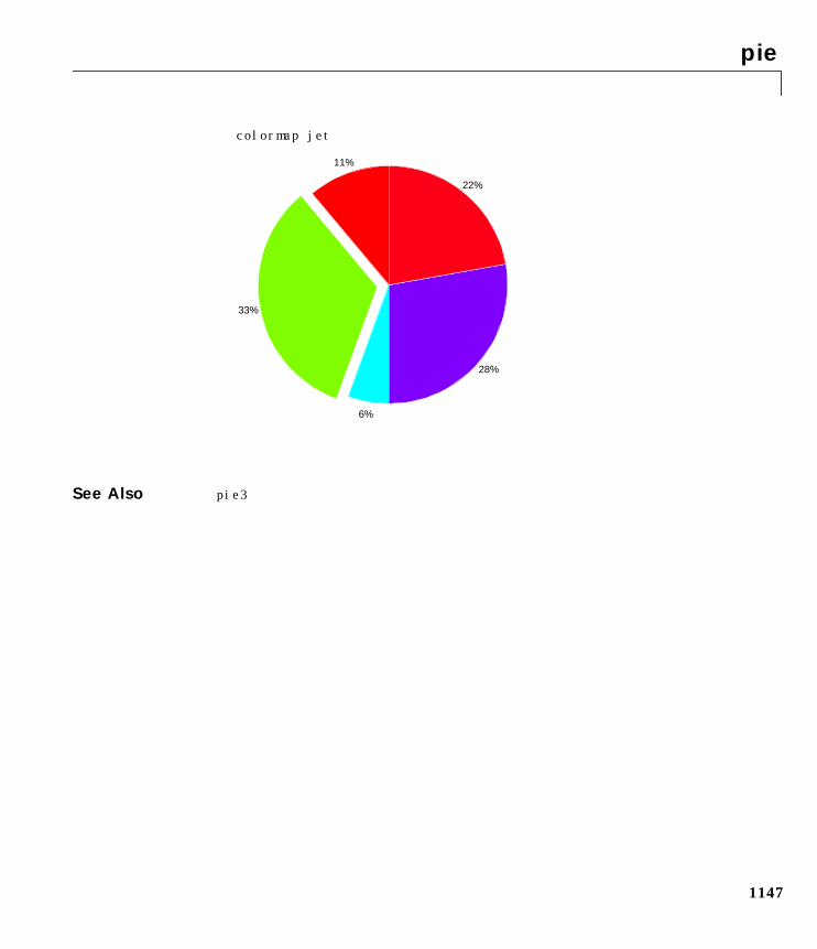
pie
1147
colormap jet
See Also pie3
11%
33%
6%
28%
22%
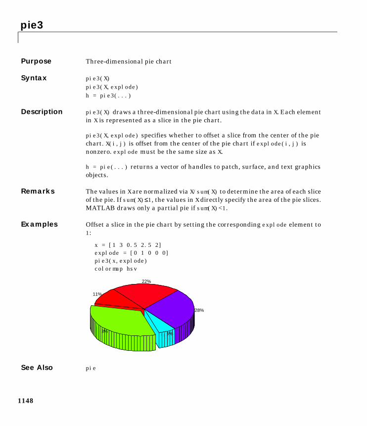
pie3
1148
1pie3Purpose Three-dimensional pie chart
Syntax pie3(X)pie3(X,explode)h = pie3(...)
Description pie3(X) draws a three-dimensional pie chart using the data in X. Each elementin X is represented as a slice in the pie chart.
pie3(X,explode) specifies whether to offset a slice from the center of the piechart. X(i,j) is offset from the center of the pie chart if explode(i,j) isnonzero. explode must be the same size as X.
h = pie(...) returns a vector of handles to patch, surface, and text graphicsobjects.
Remarks The values in X are normalized via X/sum(X) to determine the area of each sliceof the pie. If sum(X)≤1, the values in X directly specify the area of the pie slices.MATLAB draws only a partial pie if sum(X)<1.
Examples Offset a slice in the pie chart by setting the corresponding explode element to1:
x = [1 3 0.5 2.5 2]explode = [0 1 0 0 0]pie3(x,explode)colormap hsv
See Also pie
28%
6%
22%
33%
11%
pinv
1149
1pinvPurpose Moore-Penrose pseudoinverse of a matrix
Syntax B = pinv(A)B = pinv(A,tol)
Definition The Moore-Penrose pseudoinverse is a matrix B of the same dimensions as A'satisfying four conditions:
A∗B∗A = AB∗A∗B = BA∗B is HermitianB∗A is Hermitian
The computation is based on svd(A) and any singular values less than tol aretreated as zero.
Description B = pinv(A) returns the Moore-Penrose pseudoinverse of A.
B = pinv(A,tol) returns the Moore-Penrose pseudoinverse and overrides thedefault tolerance, max(size(A))*norm(A)*eps.
Examples If A is square and not singular, then pinv(A) is an expensive way to computeinv(A). If A is not square, or is square and singular, then inv(A) does not exist.In these cases, pinv(A) has some of, but not all, the properties of inv(A).
If A has more rows than columns and is not of full rank, then theoverdetermined least squares problem
minimize norm(A∗x-b)
does not have a unique solution. Two of the infinitely many solutions are
x = pinv(A)∗b
and
y = A\b
These two are distinguished by the facts that norm(x) is smaller than the normof any other solution and that y has the fewest possible nonzero components.
For example, the matrix generated by
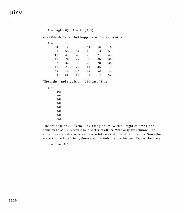
pinv
1150
A = magic(8); A = A(:,1:6)
is an 8-by-6 matrix that happens to have rank(A) = 3.
A =64 2 3 61 60 69 55 54 12 13 51
17 47 46 20 21 4340 26 27 37 36 3032 34 35 29 28 3841 23 22 44 45 1949 15 14 52 53 118 58 59 5 4 62
The right-hand side is b = 260∗ones(8,1),
b =260260260260260260260260
The scale factor 260 is the 8-by-8 magic sum. With all eight columns, onesolution to A∗x = b would be a vector of all 1’s. With only six columns, theequations are still consistent, so a solution exists, but it is not all 1’s. Since thematrix is rank deficient, there are infinitely many solutions. Two of them are
x = pinv(A)∗b
plot
1151
1plotPurpose Linear 2–D plot
Syntax plot(Y)plot(X1,Y1,...)plot(X1,Y1,LineSpec,...)plot(...,'PropertyName',PropertyValue,...)h = plot(...)
Description plot(Y) plots the columns of Y versus their index if Y is a real number. If Y iscomplex, plot(Y) is equivalent to plot(real(Y),imag(Y)). In all other uses ofplot, the imaginary component is ignored.
plot(X1,Y1,...) plots all lines defined by Xn versus Yn pairs. If only Xn or Ynis a matrix, the vector is plotted versus the rows or columns of the matrix,depending on whether the vector’s row or column dimension matches thematrix.
plot(X1,Y1,LineSpec,...) plots all lines defined by the Xn,Yn,LineSpectriples, where LineSpec is a line specification that determines line type,marker symbol, and color of the plotted lines. You can mix Xn,Yn,LineSpectriples with Xn,Yn pairs: plot(X1,Y1,X2,Y2,LineSpec,X3,Y3).
plot(...,'PropertyName',PropertyValue,...) sets properties to thespecified property values for all line graphics objects created by plot. (See the“Examples” section for examples.)
h = plot(...) returns a column vector of handles to line graphics objects, onehandle per line.
Remarks If you do not specify a color when plotting more than one line, plotautomatically cycles through the colors in the order specified by the currentaxes ColorOrder property. After cycling through all the colors defined byColorOrder, plot then cycles through the line styles defined in the axesLineStyleOrder property.
Note that, by default, MATLAB resets the ColorOrder and LineStyleOrderproperties each time you call plot. If you want changes you make to theseproperties to persist, then you must define these changes as default values. Forexample,
plot
1152
set(0,'DefaultAxesColorOrder',[0 0 0],...'DefaultAxesLineStyleOrder','-|-.|--|:')
sets the default ColorOrder to use only the color black and sets theLineStyleOrder to use solid, dash-dot, dash-dash, and dotted line styles.
Additional Information
• See the “Creating 2-D Graphs” and “Labeling Graphs” in Using MATLABGraphics for more information on plotting.
• See LineSpec for more information on specifying line styles and colors.
Examples Specifying the Color and Size of MarkersYou can also specify other line characteristics using graphics properties (seeline for a description of these properties):
• LineWidth – specifies the width (in points) of the line.
• MarkerEdgeColor – specifies the color of the marker or the edge color forfilled markers (circle, square, diamond, pentagram, hexagram, and the fourtriangles).
• MarkerFaceColor – specifies the color of the face of filled markers.
• MarkerSize – specifies the size of the marker in units of points.
For example, these statements,
x = −pi:pi/10:pi;y = tan(sin(x)) − sin(tan(x));plot(x,y,'−−rs','LineWidth',2,... 'MarkerEdgeColor','k',... 'MarkerFaceColor','g',... 'MarkerSize',10)
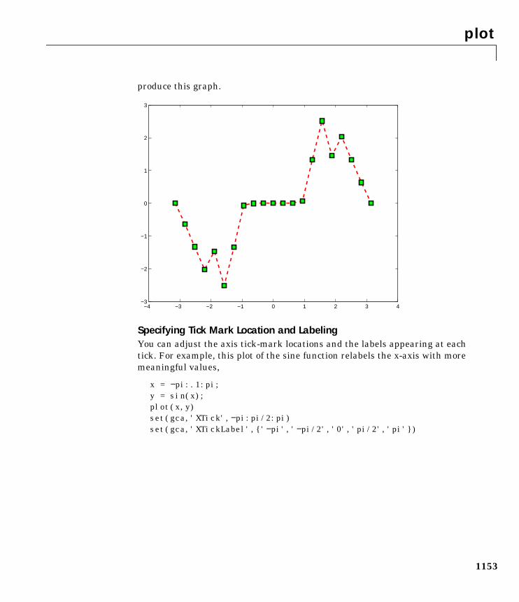
plot
1153
produce this graph.
Specifying Tick Mark Location and LabelingYou can adjust the axis tick-mark locations and the labels appearing at eachtick. For example, this plot of the sine function relabels the x-axis with moremeaningful values,
x = −pi:.1:pi;y = sin(x);plot(x,y)set(gca,'XTick',−pi:pi/2:pi)set(gca,'XTickLabel','−pi','−pi/2','0','pi/2','pi')
−4 −3 −2 −1 0 1 2 3 4−3
−2
−1
0
1
2
3
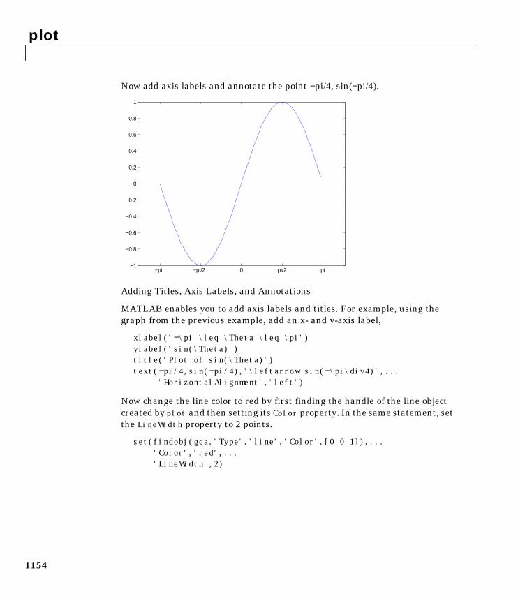
plot
1154
Now add axis labels and annotate the point −pi/4, sin(−pi/4).
Adding Titles, Axis Labels, and Annotations
MATLAB enables you to add axis labels and titles. For example, using thegraph from the previous example, add an x- and y-axis label,
xlabel('−\pi \leq \Theta \leq \pi')ylabel('sin(\Theta)')title('Plot of sin(\Theta)')text(−pi/4,sin(−pi/4),'\leftarrow sin(−\pi\div4)',...
'HorizontalAlignment','left')
Now change the line color to red by first finding the handle of the line objectcreated by plot and then setting its Color property. In the same statement, setthe LineWidth property to 2 points.
set(findobj(gca,'Type','line','Color',[0 0 1]),...'Color','red',...
'LineWidth',2)
−pi −pi/2 0 pi/2 pi−1
−0.8
−0.6
−0.4
−0.2
0
0.2
0.4
0.6
0.8
1
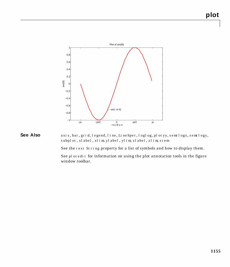
plot
1155
See Also axis, bar, grid, legend, line, LineSpec, loglog, plotyy, semilogx, semilogy,subplot, xlabel, xlim, ylabel, ylim, zlabel, zlim, stem
See the text String property for a list of symbols and how to display them.
See plotedit for information on using the plot annotation tools in the figurewindow toolbar.
−pi −pi/2 0 pi/2 pi−1
−0.8
−0.6
−0.4
−0.2
0
0.2
0.4
0.6
0.8
1
−π ≤ Θ ≤ π
sin(
Θ)
Plot of sin(Θ)
← sin(−π÷4)

plot3
1156
1plot3Purpose Linear 3-D plot
Syntax plot3(X1,Y1,Z1,...)plot3(X1,Y1,Z1,LineSpec,...)plot3(...,'PropertyName',PropertyValue,...)h = plot3(...)
Description The plot3 function displays a three-dimensional plot of a set of data points.
plot3(X1,Y1,Z1,...), where X1, Y1, Z1 are vectors or matrices, plots one ormore lines in three-dimensional space through the points whose coordinatesare the elements of X1, Y1, and Z1.
plot3(X1,Y1,Z1,LineSpec,...) creates and displays all lines defined by theXn,Yn,Zn,LineSpec quads, where LineSpec is a line specification thatdetermines line style, marker symbol, and color of the plotted lines.
plot3(...,'PropertyName',PropertyValue,...) sets properties to thespecified property values for all Line graphics objects created by plot3.
h = plot3(...) returns a column vector of handles to line graphics objects,with one handle per line.
Remarks If one or more of X1, Y1, Z1 is a vector, the vectors are plotted versus the rowsor columns of the matrix, depending whether the vectors’ lengths equal thenumber of rows or the number of columns.
You can mix Xn,Yn,Zn triples with Xn,Yn,Zn,LineSpec quads, for example,
plot3(X1,Y1,Z1,X2,Y2,Z2,LineSpec,X3,Y3,Z3)
See LineSpec and plot for information on line types and markers.
Examples Plot a three-dimensional helix.
t = 0:pi/50:10∗pi;plot3(sin(t),cos(t),t)grid onaxis square
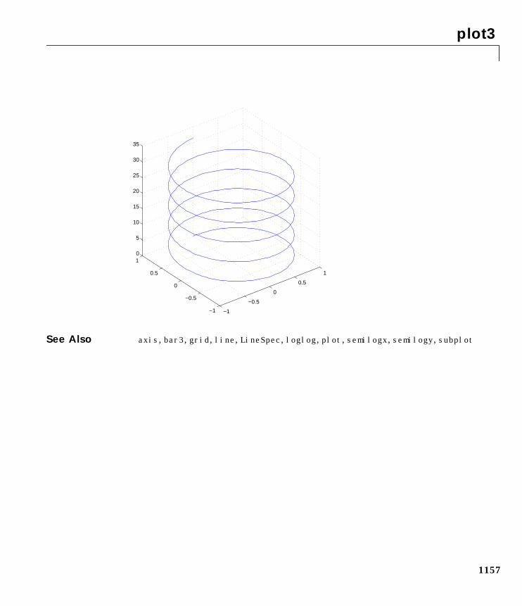
plot3
1157
See Also axis, bar3, grid, line, LineSpec, loglog, plot, semilogx, semilogy, subplot
−1
−0.5
0
0.5
1
−1
−0.5
0
0.5
10
5
10
15
20
25
30
35
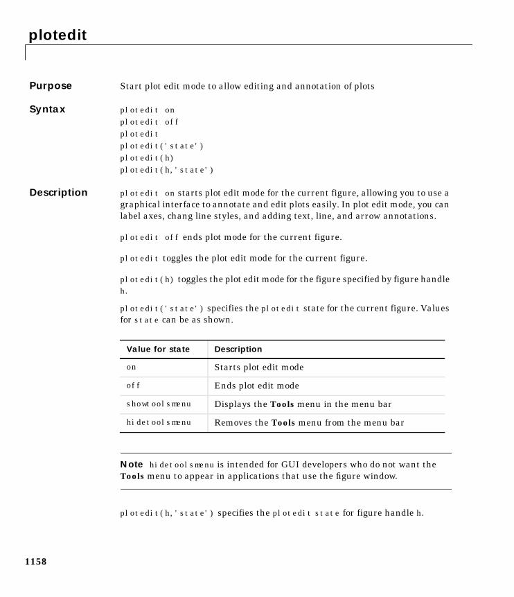
plotedit
1158
1ploteditPurpose Start plot edit mode to allow editing and annotation of plots
Syntax plotedit onplotedit offploteditplotedit('state')plotedit(h)plotedit(h,'state')
Description plotedit on starts plot edit mode for the current figure, allowing you to use agraphical interface to annotate and edit plots easily. In plot edit mode, you canlabel axes, chang line styles, and adding text, line, and arrow annotations.
plotedit off ends plot mode for the current figure.
plotedit toggles the plot edit mode for the current figure.
plotedit(h) toggles the plot edit mode for the figure specified by figure handleh.
plotedit('state') specifies the plotedit state for the current figure. Valuesfor state can be as shown.
Note hidetoolsmenu is intended for GUI developers who do not want theTools menu to appear in applications that use the figure window.
plotedit(h,'state') specifies the plotedit state for figure handle h.
Value for state Description
on Starts plot edit mode
off Ends plot edit mode
showtoolsmenu Displays the Tools menu in the menu bar
hidetoolsmenu Removes the Tools menu from the menu bar
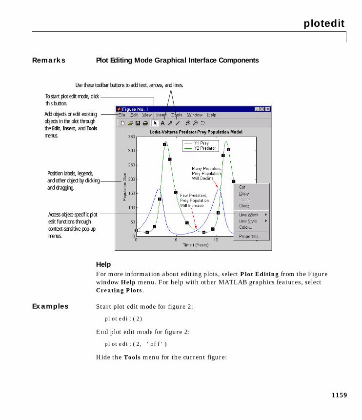
plotedit
1159
Remarks Plot Editing Mode Graphical Interface Components
HelpFor more information about editing plots, select Plot Editing from the Figurewindow Help menu. For help with other MATLAB graphics features, selectCreating Plots.
Examples Start plot edit mode for figure 2:
plotedit(2)
End plot edit mode for figure 2:
plotedit(2, 'off')
Hide the Tools menu for the current figure:
To start plot edit mode, clickthis button.
Use these toolbar buttons to add text, arrows, and lines.
Add objects or edit existingobjects in the plot throughthe Edit, Insert, and Toolsmenus.
Access object-specif ic plotedit functions throughcontext-sensitive pop-upmenus.
Position labels, legends,and other object by clickingand dragging.
plotedit
1160
plotedit('hidetoolsmenu')
See Also axes, line, open, plot, print, saveas, text, propedit
plotmatrix
1161
1plotmatrixPurpose Draw scatter plots
Syntax plotmatrix(X,Y)plotmatrix(...,'LineSpec')[H,AX,BigAx,P] = plotmatrix(...)
Description plotmatrix(X,Y) scatter plots the columns of X against the columns of Y. If Xis p-by-m and Y is p-by-n, plotmatrix produces an n-by-m matrix of axes.plotmatrix(Y) is the same as plotmatrix(Y,Y) except that the diagonal isreplaced by hist(Y(:,i)).
plotmatrix(...,'LineSpec') uses a LineSpec to create the scatter plot.Thedefault is '.' .
[H,AX,BigAx,P] = plotmatrix(...) returns a matrix of handles to the objectscreated in H, a matrix of handles to the individual subaxes in AX, a handle to abig (invisible) axes that frames the subaxes in BigAx, and a matrix of handlesfor the histogram plots in P. BigAx is left as the current axes so that asubsequent title, xlabel, or ylabel commands are centered with respect tothe matrix of axes.
Examples Generate plots of random data.
x = randn(50,3); y = x*[-1 2 1;2 0 1;1 -2 3;]';plotmatrix(y,'*r')
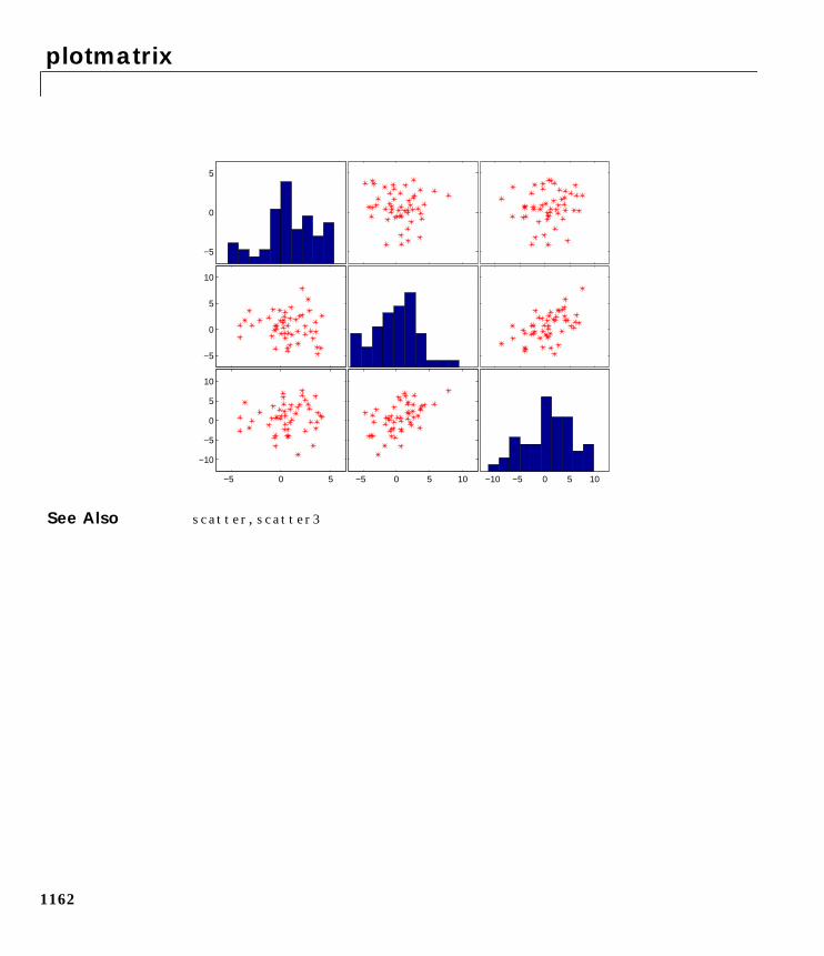
plotmatrix
1162
See Also scatter, scatter3
−10 −5 0 5 10−5 0 5 10−5 0 5
−10
−5
0
5
10
−5
0
5
10
−5
0
5
plotyy
1163
1plotyyPurpose Create graphs with y axes on both left and right side
Syntax plotyy(X1,Y1,X2,Y2)plotyy(X1,Y1,X2,Y2,'function')plotyy(X1,Y1,X2,Y2,'function1','function2')[AX,H1,H2] = plotyy(...)
Description plotyy(X1,Y1,X2,Y2) plots X1 versus Y1 with y-axis labeling on the left andplots X2 versus Y2 with y-axis labeling on the right.
plotyy(X1,Y1,X2,Y2,'function') uses the plotting function specified by thestring 'function' instead of plot to produce each graph. 'function' can be plot,semilogx, semilogy, loglog, stem or any MATLAB function that accepts thesyntax:
h = function(x,y)
plotyy(X1,Y1,X2,Y2,'function1','function2') uses function1(X1,Y1) toplot the data for the left axis and function2(X2,Y2) to plot the data for theright axis.
[AX,H1,H2] = plotyy(...) returns the handles of the two axes created in AXand the handles of the graphics objects from each plot in H1 and H2. AX(1) is theleft axes and AX(2) is the right axes.
Examples This example graphs two mathematical functions using plot as the plottingfunction. The two y-axes enable you to display both sets of data on one grapheven though relative values of the data are quite different.
x = 0:0.01:20;y1 = 200*exp(-0.05*x).*sin(x);y2 = 0.8*exp(-0.5*x).*sin(10*x);[AX,H1,H2] = plotyy(x,y1,x,y2,'plot');
You can use the handles returned by plotyy to label the axes and set the linestyles used for plotting. With the axes handles you can specify the YLabelproperties of the left- and right-side y-axis:
set(get(AX(1),'Ylabel'),'String','Left Y-axis')set(get(AX(2),'Ylabel'),'String','Right Y-axis')
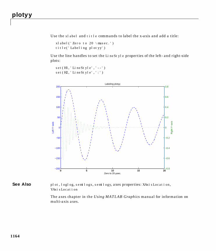
plotyy
1164
Use the xlabel and title commands to label the x-axis and add a title:
xlabel('Zero to 20 \musec.')title('Labeling plotyy')
Use the line handles to set the LineStyle properties of the left- and right-sideplots:
set(H1,'LineStyle','--')set(H2,'LineStyle',':')
See Also plot, loglog, semilogx, semilogy, axes properties: XAxisLocation,YAxisLocation
The axes chapter in the Using MATLAB Graphics manual for information onmulti-axis axes.
0 5 10 15 20−200
−150
−100
−50
0
50
100
150
200
Left
Y−
axis
Zero to 20 µsec.
Labeling plotyy
0 5 10 15 20−0.8
−0.6
−0.4
−0.2
0
0.2
0.4
0.6
0.8
Rig
ht Y
−ax
is
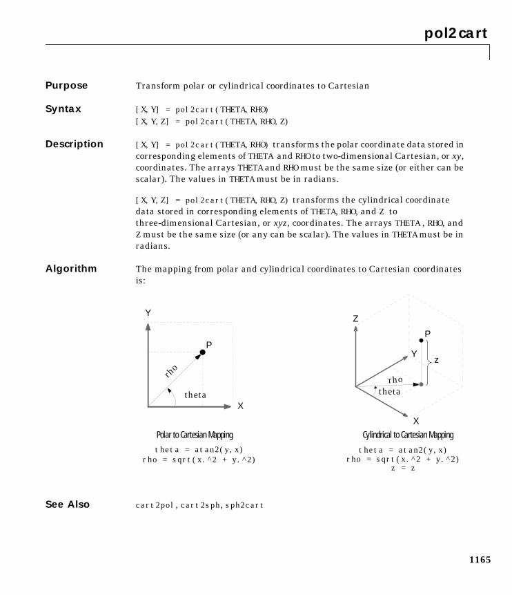
pol2cart
1165
1pol2cartPurpose Transform polar or cylindrical coordinates to Cartesian
Syntax [X,Y] = pol2cart(THETA,RHO)[X,Y,Z] = pol2cart(THETA,RHO,Z)
Description [X,Y] = pol2cart(THETA,RHO) transforms the polar coordinate data stored incorresponding elements of THETA and RHO to two-dimensional Cartesian, or xy,coordinates. The arrays THETA and RHO must be the same size (or either can bescalar). The values in THETA must be in radians.
[X,Y,Z] = pol2cart(THETA,RHO,Z) transforms the cylindrical coordinatedata stored in corresponding elements of THETA, RHO, and Z tothree-dimensional Cartesian, or xyz, coordinates. The arrays THETA , RHO, andZ must be the same size (or any can be scalar). The values in THETA must be inradians.
Algorithm The mapping from polar and cylindrical coordinates to Cartesian coordinatesis:
See Also cart2pol, cart2sph, sph2cart
theta = atan2(y,x)rho = sqrt(x.^2 + y.^2)
Cylindrical to Cartesian Mapping
Z
Y
X
rhotheta
P
z
Polar to Cartesian Mapping
P
X
Y
rho
theta
theta = atan2(y,x)rho = sqrt(x.^2 + y.^2)
z = z
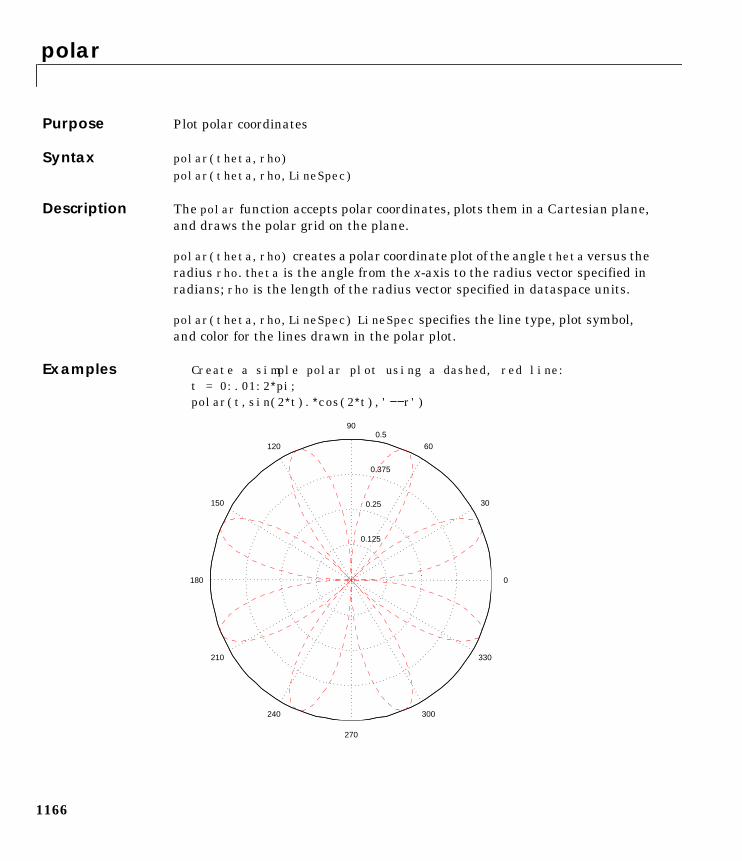
polar
1166
1polarPurpose Plot polar coordinates
Syntax polar(theta,rho)polar(theta,rho,LineSpec)
Description The polar function accepts polar coordinates, plots them in a Cartesian plane,and draws the polar grid on the plane.
polar(theta,rho) creates a polar coordinate plot of the angle theta versus theradius rho. theta is the angle from the x-axis to the radius vector specified inradians; rho is the length of the radius vector specified in dataspace units.
polar(theta,rho,LineSpec) LineSpec specifies the line type, plot symbol,and color for the lines drawn in the polar plot.
Examples Create a simple polar plot using a dashed, red line:t = 0:.01:2∗pi;polar(t,sin(2∗t).∗cos(2∗t),'−−r')
0.125
0.25
0.375
0.5
30
210
60
240
90
270
120
300
150
330
180 0

polar
1167
See Also cart2pol, compass, LineSpec, plot, pol2cart, rose
poly
1168
1polyPurpose Polynomial with specified roots
Syntax p = poly(A)p = poly(r)
Description p = poly(A) where A is an n-by-n matrix returns an n+1 element row vectorwhose elements are the coefficients of the characteristic polynomial, det(sI- A).The coefficients are ordered in descending powers: if a vector c has n+1components, the polynomial it represents is
p = poly(r) where r is a vector returns a row vector whose elements are thecoefficients of the polynomial whose roots are the elements of r.
Remarks Note the relationship of this command to
r = roots(p)
which returns a column vector whose elements are the roots of the polynomialspecified by the coefficients row vector p. For vectors, roots and poly areinverse functions of each other, up to ordering, scaling, and roundoff error.
Examples MATLAB displays polynomials as row vectors containing the coefficientsordered by descending powers. The characteristic equation of the matrix
A =
1 2 34 5 67 8 0
is returned in a row vector by poly:
p = poly(A)
p =1 -6 -72 -27
The roots of this polynomial (eigenvalues of matrix A) are returned in a columnvector by roots:
r = roots(p)
c1sn … cns cn 1++ + +
poly
1169
r =
12.1229-5.7345-0.3884
Algorithm The algorithms employed for poly and roots illustrate an interesting aspect ofthe modern approach to eigenvalue computation. poly(A) generates thecharacteristic polynomial of A, and roots(poly(A)) finds the roots of thatpolynomial, which are the eigenvalues of A. But both poly and roots use eig,which is based on similarity transformations. The classical approach, whichcharacterizes eigenvalues as roots of the characteristic polynomial, is actuallyreversed.
If A is an n-by-n matrix, poly(A) produces the coefficients c(1) throughc(n+1), with c(1) = 1, in
The algorithm is
z = eig(A);c = zeros(n+1,1); c(1) = 1;for j = 1:n
c(2:j+1) = c(2:j+1)-z(j)∗c(1:j);end
This recursion is easily derived by expanding the product.
It is possible to prove that poly(A) produces the coefficients in thecharacteristic polynomial of a matrix within roundoff error of A. This is trueeven if the eigenvalues of A are badly conditioned. The traditional algorithmsfor obtaining the characteristic polynomial, which do not use the eigenvalues,do not have such satisfactory numerical properties.
See Also conv, polyval, residue, roots
det λI A–( ) c1λn … cnλ cn 1++ + +=
λ λ1–( ) λ λ2–( )… λ λn–( )
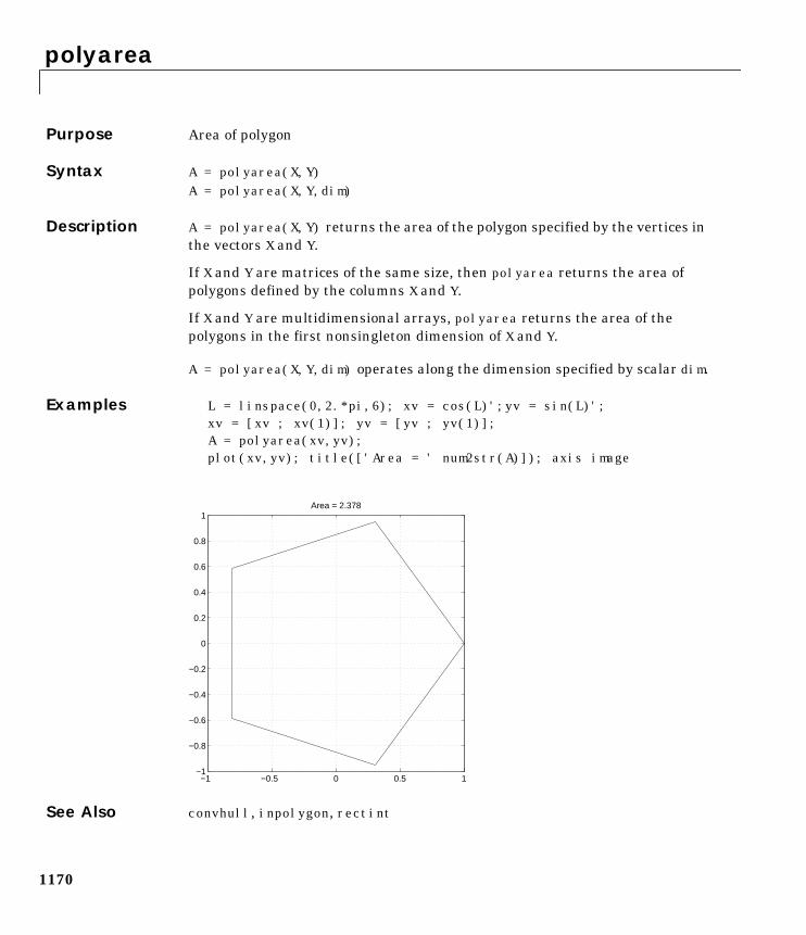
polyarea
1170
1polyareaPurpose Area of polygon
Syntax A = polyarea(X,Y)A = polyarea(X,Y,dim)
Description A = polyarea(X,Y) returns the area of the polygon specified by the vertices inthe vectors X and Y.
If X and Y are matrices of the same size, then polyarea returns the area ofpolygons defined by the columns X and Y.
If X and Y are multidimensional arrays, polyarea returns the area of thepolygons in the first nonsingleton dimension of X and Y.
A = polyarea(X,Y,dim) operates along the dimension specified by scalar dim.
Examples L = linspace(0,2.*pi,6); xv = cos(L)';yv = sin(L)';xv = [xv ; xv(1)]; yv = [yv ; yv(1)];A = polyarea(xv,yv);plot(xv,yv); title(['Area = ' num2str(A)]); axis image
See Also convhull, inpolygon, rectint
−1 −0.5 0 0.5 1−1
−0.8
−0.6
−0.4
−0.2
0
0.2
0.4
0.6
0.8
1Area = 2.378
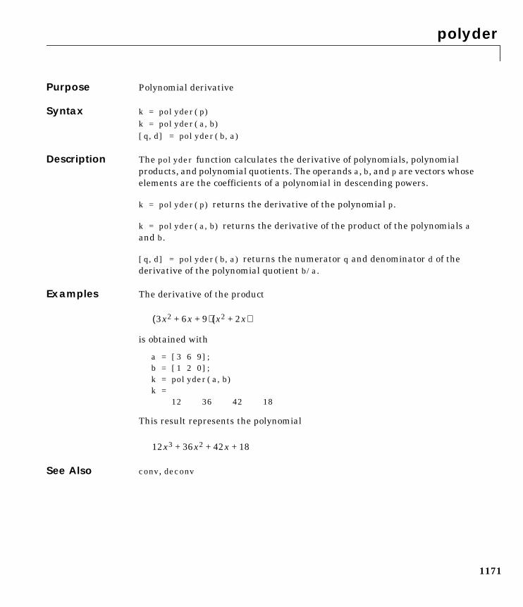
polyder
1171
1polyderPurpose Polynomial derivative
Syntax k = polyder(p)k = polyder(a,b)[q,d] = polyder(b,a)
Description The polyder function calculates the derivative of polynomials, polynomialproducts, and polynomial quotients. The operands a, b, and p are vectors whoseelements are the coefficients of a polynomial in descending powers.
k = polyder(p) returns the derivative of the polynomial p.
k = polyder(a,b) returns the derivative of the product of the polynomials aand b.
[q,d] = polyder(b,a) returns the numerator q and denominator d of thederivative of the polynomial quotient b/a.
Examples The derivative of the product
is obtained with
a = [3 6 9];b = [1 2 0];k = polyder(a,b)k =
12 36 42 18
This result represents the polynomial
See Also conv, deconv
3x2 6x 9+ +( ) x2 2x+( )
12x3 36x2 42x 18+ + +
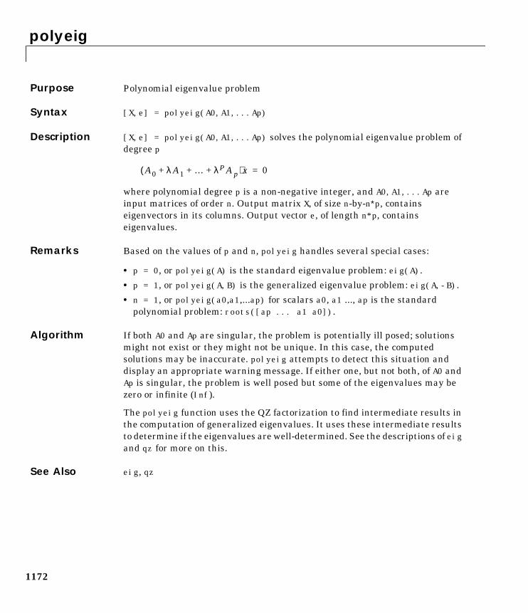
polyeig
1172
1polyeigPurpose Polynomial eigenvalue problem
Syntax [X,e] = polyeig(A0,A1,...Ap)
Description [X,e] = polyeig(A0,A1,...Ap) solves the polynomial eigenvalue problem ofdegree p
where polynomial degree p is a non-negative integer, and A0,A1,...Ap areinput matrices of order n. Output matrix X, of size n-by-n∗p, containseigenvectors in its columns. Output vector e, of length n*p, containseigenvalues.
Remarks Based on the values of p and n, polyeig handles several special cases:
• p = 0, or polyeig(A) is the standard eigenvalue problem: eig(A).
• p = 1, or polyeig(A,B) is the generalized eigenvalue problem: eig(A,-B).
• n = 1, or polyeig(a0,a1,...ap) for scalars a0, a1 ..., ap is the standardpolynomial problem: roots([ap ... a1 a0]).
Algorithm If both A0 and Ap are singular, the problem is potentially ill posed; solutionsmight not exist or they might not be unique. In this case, the computedsolutions may be inaccurate. polyeig attempts to detect this situation anddisplay an appropriate warning message. If either one, but not both, of A0 andAp is singular, the problem is well posed but some of the eigenvalues may bezero or infinite (Inf).
The polyeig function uses the QZ factorization to find intermediate results inthe computation of generalized eigenvalues. It uses these intermediate resultsto determine if the eigenvalues are well-determined. See the descriptions of eigand qz for more on this.
See Also eig, qz
A0 λ A1 … λP Ap+ + +( )x 0=
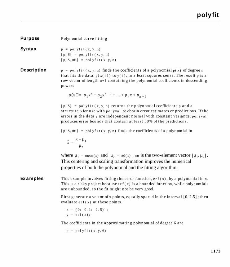
polyfit
1173
1polyfitPurpose Polynomial curve fitting
Syntax p = polyfit(x,y,n)[p,S] = polyfit(x,y,n)[p,S,mu] = polyfit(x,y,n)
Description p = polyfit(x,y,n) finds the coefficients of a polynomial p(x) of degree nthat fits the data, p(x(i)) to y(i), in a least squares sense. The result p is arow vector of length n+1 containing the polynomial coefficients in descendingpowers
[p,S] = polyfit(x,y,n) returns the polynomial coefficients p and astructure S for use with polyval to obtain error estimates or predictions. If theerrors in the data y are independent normal with constant variance, polyvalproduces error bounds that contain at least 50% of the predictions.
[p,S,mu] = polyfit(x,y,n) finds the coefficients of a polynomial in
where and .mu is the two-element vector .This centering and scaling transformation improves the numericalproperties of both the polynomial and the fitting algorithm.
Examples This example involves fitting the error function, erf(x), by a polynomial in x.This is a risky project because erf(x) is a bounded function, while polynomialsare unbounded, so the fit might not be very good.
First generate a vector of x points, equally spaced in the interval ; thenevaluate erf(x) at those points.
x = (0: 0.1: 2.5)';y = erf(x);
The coefficients in the approximating polynomial of degree 6 are
p = polyfit(x,y,6)
p x( ) p1xn p2xn 1– … pnx pn 1++ + + +=
xx µ1–
µ2---------------=
µ1 mean x( )= µ2 std x( )= µ1 µ2,[ ]
0 2.5,[ ]
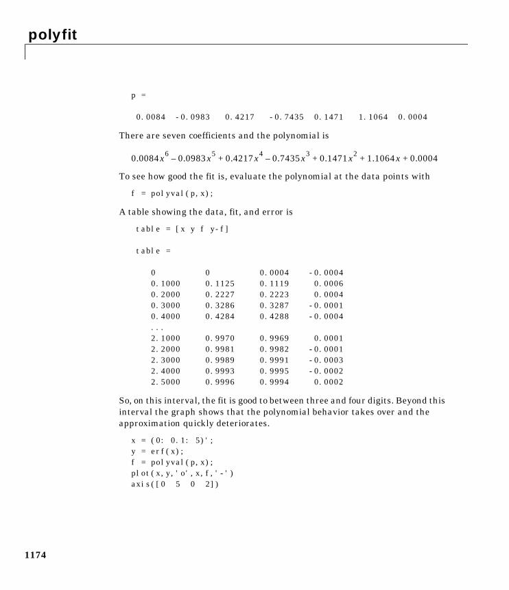
polyfit
1174
p =
0.0084 -0.0983 0.4217 -0.7435 0.1471 1.1064 0.0004
There are seven coefficients and the polynomial is
To see how good the fit is, evaluate the polynomial at the data points with
f = polyval(p,x);
A table showing the data, fit, and error is
table = [x y f y-f]
table =
0 0 0.0004 -0.00040.1000 0.1125 0.1119 0.00060.2000 0.2227 0.2223 0.00040.3000 0.3286 0.3287 -0.00010.4000 0.4284 0.4288 -0.0004...2.1000 0.9970 0.9969 0.00012.2000 0.9981 0.9982 -0.00012.3000 0.9989 0.9991 -0.00032.4000 0.9993 0.9995 -0.00022.5000 0.9996 0.9994 0.0002
So, on this interval, the fit is good to between three and four digits. Beyond thisinterval the graph shows that the polynomial behavior takes over and theapproximation quickly deteriorates.
x = (0: 0.1: 5)';y = erf(x);f = polyval(p,x);plot(x,y,'o',x,f,'-')axis([0 5 0 2])
0.0084x6 0.0983x5– 0.4217x4 0.7435x3
– 0.1471x2 1.1064x 0.0004+ + + +
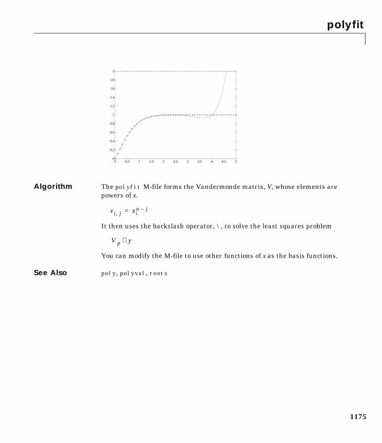
polyfit
1175
Algorithm The polyfit M-file forms the Vandermonde matrix, V, whose elements arepowers of x.
It then uses the backslash operator, \, to solve the least squares problem
You can modify the M-file to use other functions of x as the basis functions.
See Also poly, polyval, roots
0
0.2
0.4
0.6
0.8
1
1.2
1.4
1.6
1.8
2
0 0.5 1 1.5 2 2.5 3 3.5 4 4.5 5o
o
o
o
o
o
oo
oo
oo o o o o o o o o o o o o o o o o o o o o o o o o o o o o o o o o o o o o o o o
vi j, xin j–=
V p y≅
polyint
1176
1polyintPurpose Integrate polynomial analytically
Syntax polyint(p,k)polyint(p)
Description polyint(p,k) returns a polynomial representing the integral of polynomial p,using a scalar constant of integration k.
polyint(p) assumes a constant of integration k=0.
See Also polyder, polyval, polyvalm, polyfit
polyval
1177
1polyvalPurpose Polynomial evaluation
Syntax y = polyval(p,x)y = polyval(p,x,[],mu)[y,delta] = polyval(p,x,S)[y,delta] = polyval(p,x,S,mu)
Description y = polyval(p,x) returns the value of a polynomial of degree n evaluated atx. The input argument p is a vector of length n+1 whose elements are thecoefficients in descending powers of the polynomial to be evaluated.
x can be a matrix or a vector. In either case, polyval evaluates p at eachelement of x.
y = polyval(p,x,[],mu) uses in place of . In this equation, and . The centering and scaling parameters
mu = are optional output computed by polyfit.
[y,delta] = polyval(p,x,S) and [y,delta] = polyval(p,x,S,mu) use theoptional output structure S generated by polyfit to generate error estimates,y±delta. If the errors in the data input to polyfit are independent normalwith constant variance, y±delta contains at least 50% of the predictions.
Remarks The polyvalm(p,x) function, with x a matrix, evaluates the polynomial in amatrix sense. See polyvalm for more information.
Examples The polynomial is evaluated at x = 5, 7, and 9 with
p = [3 2 1];polyval(p,[5 7 9])
which results in
ans =
86 162 262
For another example, see polyfit.
y p1xn p2xn 1– … pnx pn 1++ + + +=
x x µ1–( ) µ2⁄= xµ1 mean x( )= µ2 std x( )=
µ1 µ2,[ ]
p x( ) 3x2 2x 1+ +=

polyval
1178
See Also polyfit, polyvalm
polyvalm
1179
1polyvalmPurpose Matrix polynomial evaluation
Syntax Y = polyvalm(p,X)
Description Y = polyvalm(p,X) evaluates a polynomial in a matrix sense. This is the sameas substituting matrix X in the polynomial p.
Polynomial p is a vector whose elements are the coefficients of a polynomial indescending powers, and X must be a square matrix.
Examples The Pascal matrices are formed from Pascal’s triangle of binomial coefficients.Here is the Pascal matrix of order 4.
X = pascal(4)X =
1 1 1 11 2 3 41 3 6 101 4 10 20
Its characteristic polynomial can be generated with the poly function.
p = poly(X)p =
1 -29 72 -29 1
This represents the polynomial .
Pascal matrices have the curious property that the vector of coefficients of thecharacteristic polynomial is palindromic; it is the same forward and backward.
Evaluating this polynomial at each element is not very interesting.
polyval(p,X)ans =
16 16 16 1616 15 -140 -56316 -140 -2549 -1208916 -563 -12089 -43779
But evaluating it in a matrix sense is interesting.
polyvalm(p,X)
x4 29x3– 72x2 29x– 1+ +
polyvalm
1180
ans =0 0 0 00 0 0 00 0 0 00 0 0 0
The result is the zero matrix. This is an instance of the Cayley-Hamiltontheorem: a matrix satisfies its own characteristic equation.
See Also polyfit, polyval
pow2
1181
1pow2Purpose Base 2 power and scale floating-point numbers
Syntax X = pow2(Y)X = pow2(F,E)
Description X = pow2(Y) returns an array X whose elements are 2 raised to the power Y.
X = pow2(F,E) computes for corresponding elements of F and E. Theresult is computed quickly by simply adding E to the floating-point exponent ofF. Arguments F and E are real and integer arrays, respectively.
Remarks This function corresponds to the ANSI C function ldexp() and the IEEEfloating-point standard function scalbn().
Examples For IEEE arithmetic, the statement X = pow2(F,E) yields the values:
F E X1/2 1 1pi/4 2 pi-3/4 2 -31/2 -51 eps1-eps/2 1024 realmax1/2 -1021 realmin
See Also log2, exp, hex2num, realmax, realmin
The arithmetic operators ^ and .^
x f 2e⋅=
ppval
1182
1ppvalPurpose Evaluate piecewise polynomial.
Syntax v = ppval(pp,xx)v = ppval(xx,pp)
Description v = ppval(pp,xx) returns the value at the points xx of the piecewisepolynomial contained in pp, as constructed by spline (or the spline utilitymkpp).
v = ppval(xx,pp) returns the same result and may be used with functionfunctions like fminbnd, fzero and quad.
Examples This command provides an estimate of the integral over the interval [a .. b]of the piecewise polynomial pp.
int = quad('ppval',a,b,tol,[],pp);
See Also ppval, spline, unmkpp
primes
1183
1primesPurpose Generate list of prime numbers
Syntax p = primes(n)
Description p = primes(n) returns a row vector of the prime numbers less than or equalto n. A prime number is one that has no factors other than 1 and itself.
Examples p = primes(37)
p =
2 3 5 7 11 13 17 19 23 29 31 37
See Also factor
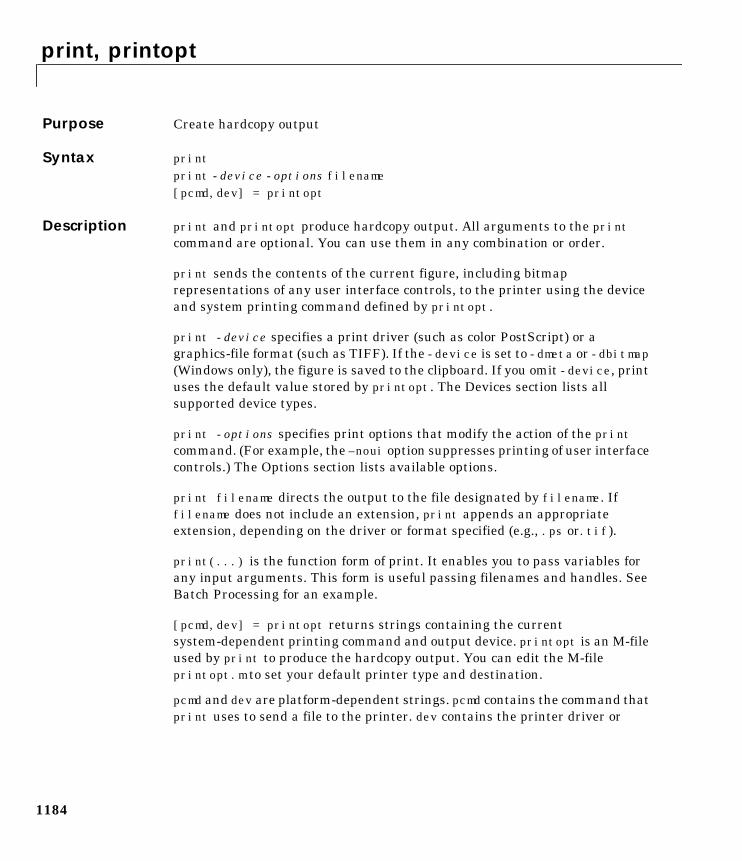
print, printopt
1184
1print, printoptPurpose Create hardcopy output
Syntax printprint -device -options filename[pcmd,dev] = printopt
Description print and printopt produce hardcopy output. All arguments to the printcommand are optional. You can use them in any combination or order.
print sends the contents of the current figure, including bitmaprepresentations of any user interface controls, to the printer using the deviceand system printing command defined by printopt.
print -device specifies a print driver (such as color PostScript) or agraphics-file format (such as TIFF). If the -device is set to -dmeta or -dbitmap(Windows only), the figure is saved to the clipboard. If you omit -device, printuses the default value stored by printopt. The Devices section lists allsupported device types.
print -options specifies print options that modify the action of the printcommand. (For example, the –noui option suppresses printing of user interfacecontrols.) The Options section lists available options.
print filename directs the output to the file designated by filename. Iffilename does not include an extension, print appends an appropriateextension, depending on the driver or format specified (e.g., .ps or.tif).
print(...) is the function form of print. It enables you to pass variables forany input arguments. This form is useful passing filenames and handles. SeeBatch Processing for an example.
[pcmd,dev] = printopt returns strings containing the currentsystem-dependent printing command and output device. printopt is an M-fileused by print to produce the hardcopy output. You can edit the M-fileprintopt.m to set your default printer type and destination.
pcmd and dev are platform-dependent strings. pcmd contains the command thatprint uses to send a file to the printer. dev contains the printer driver or
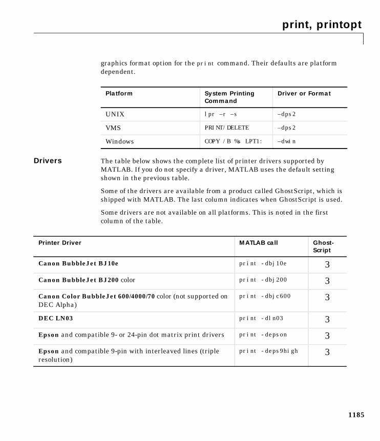
print, printopt
1185
graphics format option for the print command. Their defaults are platformdependent.
Drivers The table below shows the complete list of printer drivers supported byMATLAB. If you do not specify a driver, MATLAB uses the default settingshown in the previous table.
Some of the drivers are available from a product called GhostScript, which isshipped with MATLAB. The last column indicates when GhostScript is used.
Some drivers are not available on all platforms. This is noted in the firstcolumn of the table.
Platform System PrintingCommand
Driver or Format
UNIX lpr –r –s –dps2
VMS PRINT/DELETE –dps2
Windows COPY /B %s LPT1: –dwin
Printer Driver MATLAB call Ghost-Script
Canon BubbleJet BJ10e print -dbj10e 3
Canon BubbleJet BJ200 color print -dbj200 3
Canon Color BubbleJet 600/4000/70 color (not supported onDEC Alpha)
print -dbjc600 3
DEC LN03 print -dln03 3
Epson and compatible 9- or 24-pin dot matrix print drivers print -depson 3
Epson and compatible 9-pin with interleaved lines (tripleresolution)
print -deps9high 3
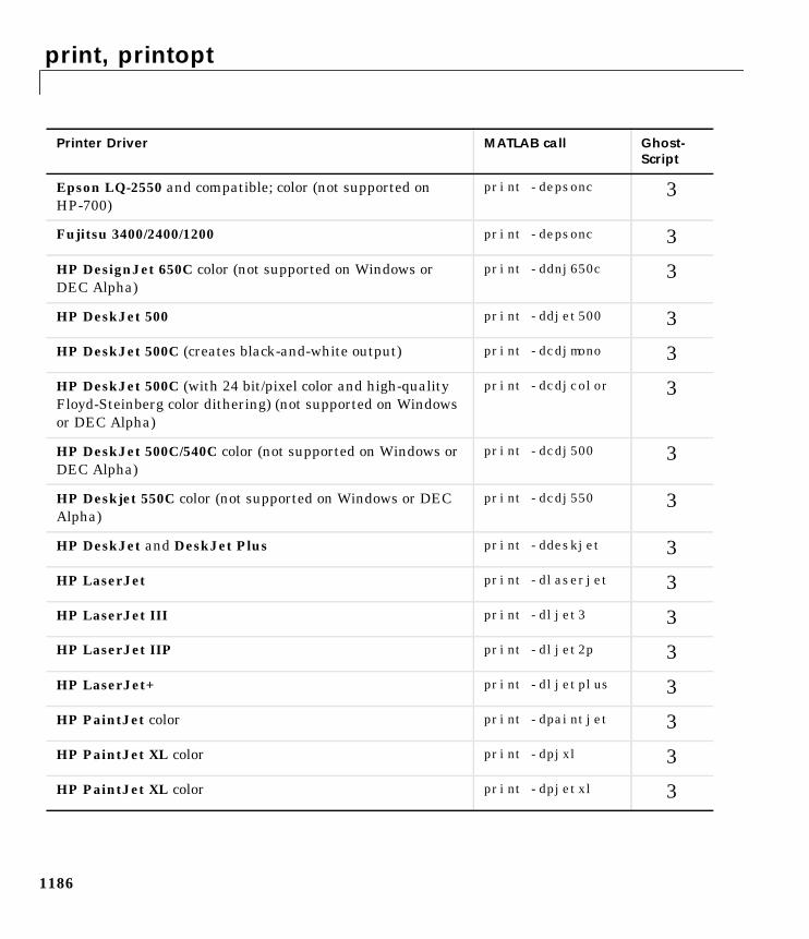
print, printopt
1186
Epson LQ-2550 and compatible; color (not supported onHP-700)
print -depsonc 3
Fujitsu 3400/2400/1200 print -depsonc 3
HP DesignJet 650C color (not supported on Windows orDEC Alpha)
print -ddnj650c 3
HP DeskJet 500 print -ddjet500 3
HP DeskJet 500C (creates black-and-white output) print -dcdjmono 3
HP DeskJet 500C (with 24 bit/pixel color and high-qualityFloyd-Steinberg color dithering) (not supported on Windowsor DEC Alpha)
print -dcdjcolor 3
HP DeskJet 500C/540C color (not supported on Windows orDEC Alpha)
print -dcdj500 3
HP Deskjet 550C color (not supported on Windows or DECAlpha)
print -dcdj550 3
HP DeskJet and DeskJet Plus print -ddeskjet 3
HP LaserJet print -dlaserjet 3
HP LaserJet III print -dljet3 3
HP LaserJet IIP print -dljet2p 3
HP LaserJet+ print -dljetplus 3
HP PaintJet color print -dpaintjet 3
HP PaintJet XL color print -dpjxl 3
HP PaintJet XL color print -dpjetxl 3
Printer Driver MATLAB call Ghost-Script
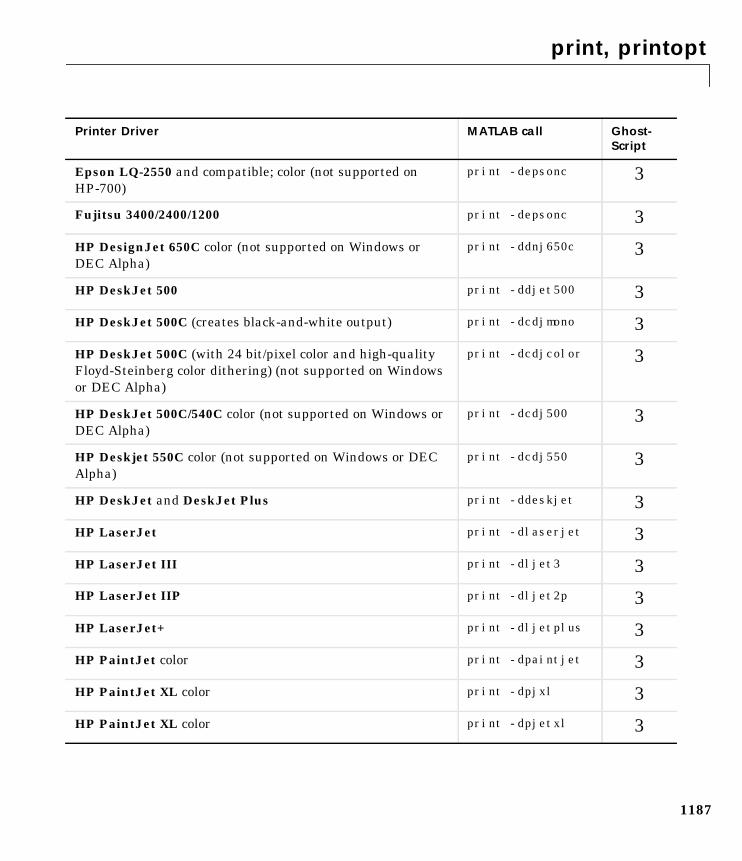
print, printopt
1187
Epson LQ-2550 and compatible; color (not supported onHP-700)
print -depsonc 3
Fujitsu 3400/2400/1200 print -depsonc 3
HP DesignJet 650C color (not supported on Windows orDEC Alpha)
print -ddnj650c 3
HP DeskJet 500 print -ddjet500 3
HP DeskJet 500C (creates black-and-white output) print -dcdjmono 3
HP DeskJet 500C (with 24 bit/pixel color and high-qualityFloyd-Steinberg color dithering) (not supported on Windowsor DEC Alpha)
print -dcdjcolor 3
HP DeskJet 500C/540C color (not supported on Windows orDEC Alpha)
print -dcdj500 3
HP Deskjet 550C color (not supported on Windows or DECAlpha)
print -dcdj550 3
HP DeskJet and DeskJet Plus print -ddeskjet 3
HP LaserJet print -dlaserjet 3
HP LaserJet III print -dljet3 3
HP LaserJet IIP print -dljet2p 3
HP LaserJet+ print -dljetplus 3
HP PaintJet color print -dpaintjet 3
HP PaintJet XL color print -dpjxl 3
HP PaintJet XL color print -dpjetxl 3
Printer Driver MATLAB call Ghost-Script
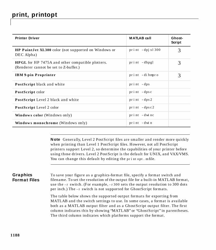
print, printopt
1188
Note Generally, Level 2 PostScript files are smaller and render more quicklywhen printing than Level 1 PostScript files. However, not all PostScriptprinters support Level 2, so determine the capabilities of your printer beforeusing those drivers. Level 2 PostScript is the default for UNIX, and VAX/VMS.You can change this default by editing the printopt.m file.
GraphicsFormat Files
To save your figure as a graphics-format file, specify a format switch andfilename. To set the resolution of the output file for a built-in MATLAB format,use the -r switch. (For example, -r300 sets the output resolution to 300 dotsper inch.) The -r switch is not supported for GhostScript formats.
The table below shows the supported output formats for exporting fromMATLAB and the switch settings to use. In some cases, a format is availableboth as a MATLAB output filter and as a GhostScript output filter. The firstcolumn indicates this by showing “MATLAB” or “GhostScript” in parentheses.The third column indicates which platforms support the format.
HP PaintJet XL300 color (not supported on Windows orDEC Alpha)
print -dpjxl300 3
HPGL for HP 7475A and other compatible plotters.(Renderer cannot be set to Z-buffer.)
print -dhpgl 3
IBM 9-pin Proprinter print -dibmpro 3
PostScript black and white print -dps
PostScript color print -dpsc
PostScript Level 2 black and white print -dps2
PostScript Level 2 color print -dpsc2
Windows color (Windows only) print -dwinc
Windows monochrome (Windows only) print -dwin
Printer Driver MATLAB call Ghost-Script
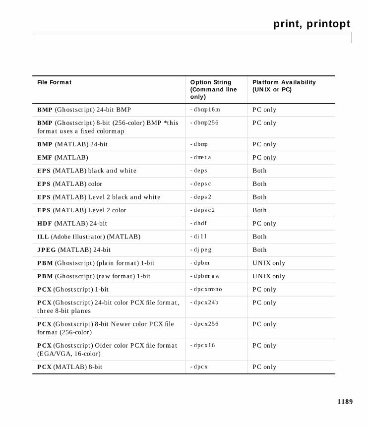
print, printopt
1189
File Format Option String(Command lineonly)
Platform Availability(UNIX or PC)
BMP (Ghostscript) 24-bit BMP -dbmp16m PC only
BMP (Ghostscript) 8-bit (256-color) BMP *thisformat uses a fixed colormap
-dbmp256 PC only
BMP (MATLAB) 24-bit -dbmp PC only
EMF (MATLAB) -dmeta PC only
EPS (MATLAB) black and white -deps Both
EPS (MATLAB) color -depsc Both
EPS (MATLAB) Level 2 black and white -deps2 Both
EPS (MATLAB) Level 2 color -depsc2 Both
HDF (MATLAB) 24-bit -dhdf PC only
ILL (Adobe Illustrator) (MATLAB) -dill Both
JPEG (MATLAB) 24-bit -djpeg Both
PBM (Ghostscript) (plain format) 1-bit -dpbm UNIX only
PBM (Ghostscript) (raw format) 1-bit -dpbmraw UNIX only
PCX (Ghostscript) 1-bit -dpcxmono PC only
PCX (Ghostscript) 24-bit color PCX file format,three 8-bit planes
-dpcx24b PC only
PCX (Ghostscript) 8-bit Newer color PCX fileformat (256-color)
-dpcx256 PC only
PCX (Ghostscript) Older color PCX file format(EGA/VGA, 16-color)
-dpcx16 PC only
PCX (MATLAB) 8-bit -dpcx PC only
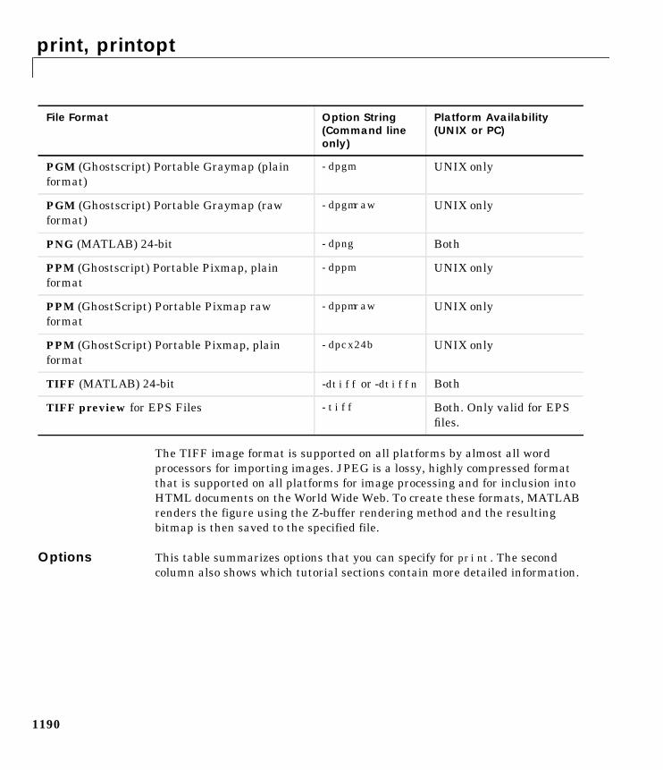
print, printopt
1190
The TIFF image format is supported on all platforms by almost all wordprocessors for importing images. JPEG is a lossy, highly compressed formatthat is supported on all platforms for image processing and for inclusion intoHTML documents on the World Wide Web. To create these formats, MATLABrenders the figure using the Z-buffer rendering method and the resultingbitmap is then saved to the specified file.
Options This table summarizes options that you can specify for print. The secondcolumn also shows which tutorial sections contain more detailed information.
PGM (Ghostscript) Portable Graymap (plainformat)
-dpgm UNIX only
PGM (Ghostscript) Portable Graymap (rawformat)
-dpgmraw UNIX only
PNG (MATLAB) 24-bit -dpng Both
PPM (Ghostscript) Portable Pixmap, plainformat
-dppm UNIX only
PPM (GhostScript) Portable Pixmap rawformat
-dppmraw UNIX only
PPM (GhostScript) Portable Pixmap, plainformat
-dpcx24b UNIX only
TIFF (MATLAB) 24-bit -dtiff or -dtiffn Both
TIFF preview for EPS Files -tiff Both. Only valid for EPSfiles.
File Format Option String(Command lineonly)
Platform Availability(UNIX or PC)
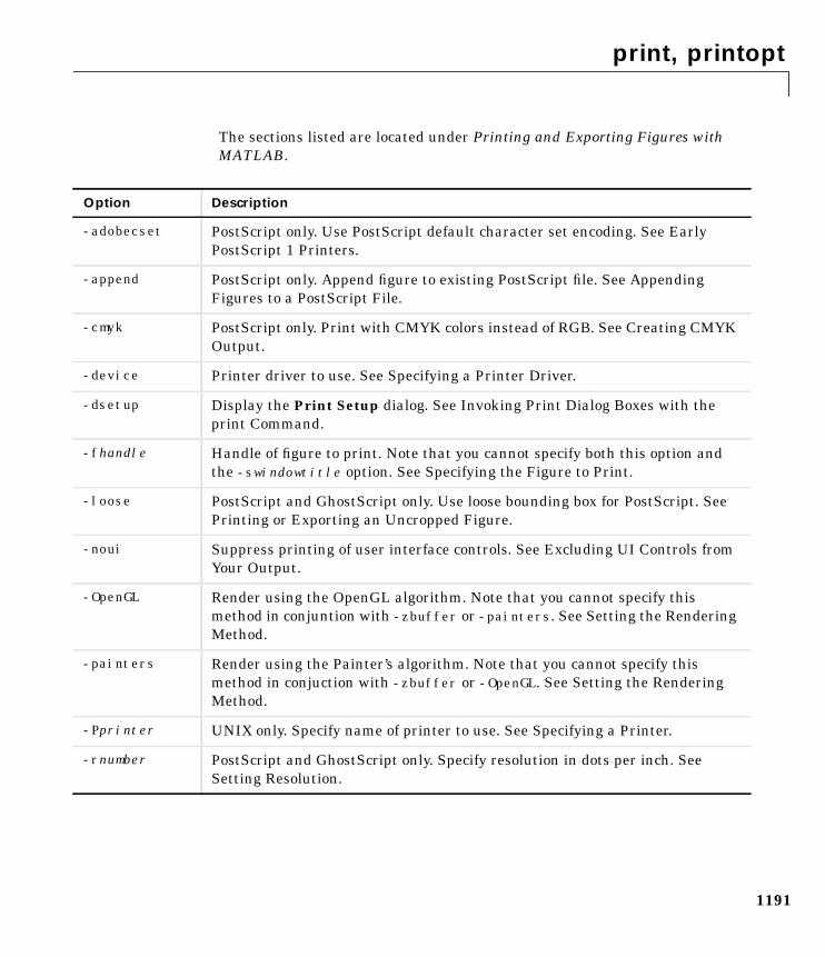
print, printopt
1191
The sections listed are located under Printing and Exporting Figures withMATLAB.
Option Description
-adobecset PostScript only. Use PostScript default character set encoding. See EarlyPostScript 1 Printers.
-append PostScript only. Append figure to existing PostScript file. See AppendingFigures to a PostScript File.
-cmyk PostScript only. Print with CMYK colors instead of RGB. See Creating CMYKOutput.
-device Printer driver to use. See Specifying a Printer Driver.
-dsetup Display the Print Setup dialog. See Invoking Print Dialog Boxes with theprint Command.
-fhandle Handle of figure to print. Note that you cannot specify both this option andthe -swindowtitle option. See Specifying the Figure to Print.
-loose PostScript and GhostScript only. Use loose bounding box for PostScript. SeePrinting or Exporting an Uncropped Figure.
-noui Suppress printing of user interface controls. See Excluding UI Controls fromYour Output.
-OpenGL Render using the OpenGL algorithm. Note that you cannot specify thismethod in conjuntion with -zbuffer or -painters. See Setting the RenderingMethod.
-painters Render using the Painter’s algorithm. Note that you cannot specify thismethod in conjuction with -zbuffer or -OpenGL. See Setting the RenderingMethod.
-Pprinter UNIX only. Specify name of printer to use. See Specifying a Printer.
-rnumber PostScript and GhostScript only. Specify resolution in dots per inch. SeeSetting Resolution.
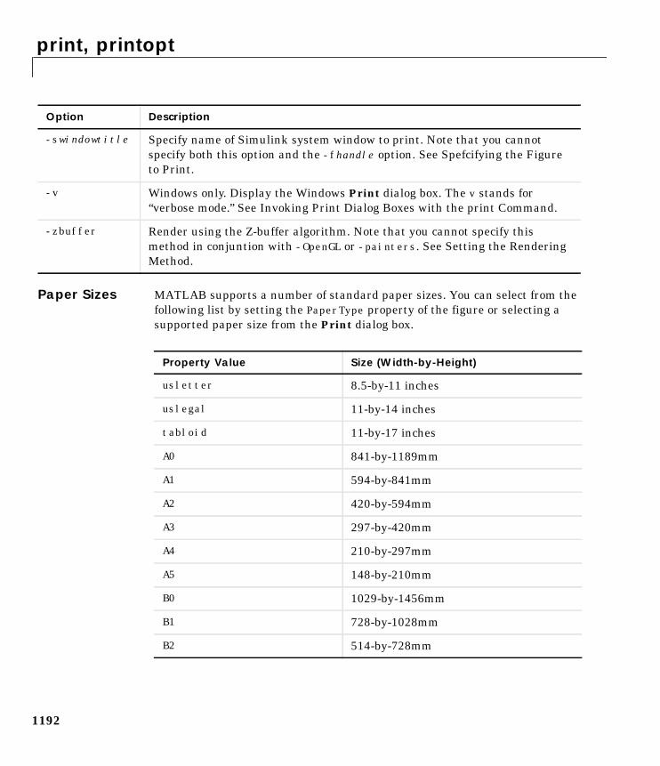
print, printopt
1192
Paper Sizes MATLAB supports a number of standard paper sizes. You can select from thefollowing list by setting the PaperType property of the figure or selecting asupported paper size from the Print dialog box.
-swindowtitle Specify name of Simulink system window to print. Note that you cannotspecify both this option and the -fhandle option. See Spefcifying the Figureto Print.
-v Windows only. Display the Windows Print dialog box. The v stands for“verbose mode.” See Invoking Print Dialog Boxes with the print Command.
-zbuffer Render using the Z-buffer algorithm. Note that you cannot specify thismethod in conjuntion with -OpenGL or -painters. See Setting the RenderingMethod.
Option Description
Property Value Size (Width-by-Height)
usletter 8.5-by-11 inches
uslegal 11-by-14 inches
tabloid 11-by-17 inches
A0 841-by-1189mm
A1 594-by-841mm
A2 420-by-594mm
A3 297-by-420mm
A4 210-by-297mm
A5 148-by-210mm
B0 1029-by-1456mm
B1 728-by-1028mm
B2 514-by-728mm
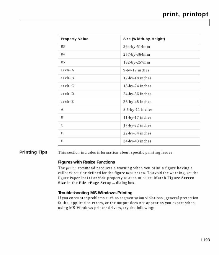
print, printopt
1193
Printing Tips This section includes information about specific printing issues.
Figures with Resize FunctionsThe print command produces a warning when you print a figure having acallback routine defined for the figure ResizeFcn. To avoid the warning, set thefigure PaperPositionMode property to auto or select Match Figure ScreenSize in the File->Page Setup... dialog box.
Troubleshooting MS-Windows PrintingIf you encounter problems such as segmentation violations , general protectionfaults, application errors, or the output does not appear as you expect whenusing MS-Windows printer drivers, try the following:
B3 364-by-514mm
B4 257-by-364mm
B5 182-by-257mm
arch-A 9-by-12 inches
arch-B 12-by-18 inches
arch-C 18-by-24 inches
arch-D 24-by-36 inches
arch-E 36-by-48 inches
A 8.5-by-11 inches
B 11-by-17 inches
C 17-by-22 inches
D 22-by-34 inches
E 34-by-43 inches
Property Value Size (Width-by-Height)
print, printopt
1194
• If your printer is PostScript compatible, print with one of MATLAB’s built-inPostScript drivers. There are various PostScript device options that you canuse with the print command: they all start with −dps.
• The behavior you are experiencing may occur only with certain versions ofthe print driver. Contact the print driver vendor for information on how toobtain and install a different driver. If you are using Windows 95, tryinstalling the drivers that ship with the Windows 95 CD-ROM.
• Try printing with one of MATLAB’s built-in GhostScript devices. Thesedevices use GhostScript to convert PostScript files into other formats, suchas HP LaserJet, PCX, Canon BubbleJet, and so on.
• Copy the figure as a Windows Metafile using the Edit-->Copy Figure menuitem on the figure window menu or the print −dmeta option at the commandline. You can then import the file into another application for printing.
You can set copy options in the figure’s File-->Preferences...-->CopyingOptions dialog box. The Windows Metafile clipboard format produces abetter quality image than Windows Bitmap.
Printing Thick Lines on Windows95Due to a limitation in Windows95, MATLAB is set up to print lines as either:
• Solid lines of the specified thickness (LineWidth)
• Thin (one pixel wide) lines with the specified line style (LineStyle)
If you create lines that are thicker than one pixel and use nonsolid line styles,MATLAB prints these lines with the specified line style, but one pixel wide (i.e.,as thin lines).
However, you can change this behavior so that MATLAB prints thick, styledlines as thick, solid lines by editing your matlab.ini file, which is in yourWindows directory. In this file, find the section,
[Matlab Settings]
and in this section change the assignment,
ThinLineStyles=1to
ThinLineStyles=0
then restart MATLAB.
print, printopt
1195
Printing MATLAB GUIsYou can generally obtain better results when printing a figure window thatcontains MATLAB uicontrols by setting these key properties:
• Set the figure PaperPositionMode property to auto. This ensures the printedversion is the same size as the onscreen version. With PaperPositionModeset to auto MATLAB does not resize the figure to fit the current value of thePaperPosition. This is particularly important if you have specified a figureResizeFcn because if MATLAB resizes the figure during the print operation,the ResizeFcn is automatically called.
To set PaperPositionMode on the current figure, use the command:set(gcf,'PaperPositionMode','auto')
• Set the figure InvertHardcopy property to off. By default, MATLABchanges the figure background color of printed output to white, but does notchange the color of uicontrols. If you have set the background color to, forexample, match the gray of the GUI devices, you must set InvertHardcopyto off to preserve the color scheme.
To set InvertHardcopy on the current figure, use the command:set(gcf,'InvertHardcopy','off')
• Use a color device if you want lines and text that are in color on the screen tobe written to the output file as colored objects. Black and white devicesconvert colored lines and text to black or white to provide the best contrastwith the background and to aviod dithering.
• Use the print command’s −loose option to prevent MATLAB from using abounding box that is tightly wrapped around objects contained in the figure.This is important if you have intentionally used space between uicontrols oraxes and the edge of the figure and you want to maintain this appearance inthe printed output.
Notes on Printing Interpolated Shading with PostScript DriversMATLAB can print surface objects (such as graphs created with surf or mesh)using interpolated colors. However, only patch objects that are composed oftriangular faces can be printed using interpolated shading.
Printed output is always interpolated in RGB space, not in the colormap colors.This means, if you are using indexed color and interpolated face coloring, theprinted output can look different from what is displayed on screen.
print, printopt
1196
PostScript files generated for interpolated shading contain the colorinformation of the graphics object’s vertices and require the printer to performthe interpolation calculations. This can take an excessive amount of time andin some cases, printers may actually “time-out” before finishing the print job.One solution to this problem is to interpolate the data and generate a greaternumber of faces, which can then be flat shaded.
To ensure that the printed output matches what you see on the screen, printusing the -zbuffer option. To obtain higher resolution (for example, to maketext look better), use the −r option to increase the resolution. There is, however,a trade-off between the resolution and the size of the created PostScript file,which can be quite large at higher resolutions. The default resolution of 150 dpigenerally produces good results. You can reduce the size of the output file bymaking the figure smaller before printing it and setting the figurePaperPositionMode to auto, or by just setting the PaperPosition property toa smaller size.
Note that in some UNIX environments, the default lpr command cannot printfiles larger than 1 Mbyte unless you use the −s option, which MATLAB doesby default. See the lpr man page for more information.
Examples Specifying the Figure to PrintYou can print a noncurrent figure by specifying the figure’s handle. If a figurehas the title “Figure No. 2”, its handle is 2. The syntax is,
print -fhandle
This example prints the figure whose handle is 2, regardless of which figure isthe current figure.
print -f2
Note Note that you must use the -f option if the figure’s handle is hidden(i.e., its HandleVisibility property is set to off).
print, printopt
1197
This example saves the figure with the handle -f2 to a PostScript file namedFigure2, which can be printed later.
print -f2 -dps 'Figure2.ps'
If the figure uses noninteger handles, use the figure command to get its value,and then pass it in as the first argument.
h = figure('IntegerHandle','off')print h -depson
You can also pass a figure handle as a variable to the function form of print.For example,
h = figure; plot(1:4,5:8)print(h)
This example uses the function form of print to enable a filename to be passedin as a variable.
filename = 'mydata';print('-f3', '-dpsc', filename);
(Because a filename is specified, the figure will be printed to a file.)
Specifying the Model to PrintTo print a noncurrent Simulink model, use the -s option with the title of thewindow. For example, this command prints the Simulink window titled f14.
print -sf14
If the window title includes any spaces, you must call the function form ratherthan the command form of print. For example, this command saves a Simulinkwindow title Thruster Control.
print('-sThruster Control')
To print the current system use:
print -s
For information about issues specific to printing Simulink windows, see theSimulink documentation.
print, printopt
1198
This example prints a surface plot with interpolated shading. Setting thecurrent figure’s (gcf) PaperPositionMode to auto enables you to resize thefigure window and print it at the size you see on the screen. See Options andthe previous section for information on the −zbuffer and −r200 options.
surf(peaks)shading interpset(gcf,'PaperPositionMode','auto')print −dpsc2 −zbuffer −r200
Batch ProcessingYou can use the function form of print to pass variables containing file names.For example, this for loop creates a series of graphs and prints each one with adifferent file name.
for i=1:length(fnames)surf(Z(:,:,i))print('-dtiff','-r200',fnames(i))
end
Tiff PreviewThe command:
print -depsc -tiff -r300 picture1
saves the current figure at 300 dpi, in a color Encapsulated PostScript filenamed picture1.eps. The -tiff option creates a 72 dpi TIFF preview, whichmany word processor applications can display on screen after you import theEPS file. This enables you to view the picture on screen within your wordprocessor and print the document to a PostScript printer using a resolution of300 dpi.
See Also orient, figure
printdlg
1199
1printdlgPurpose Display print dialog box
Syntax printdlgprintdlg(fig)printdlg('-crossplatform’,fig)printdlg('-setup’,fig)
Description printdlg prints the current figure.
printdlg(fig) creates a dialog box from which you can print the figurewindow identified by the handle fig. Note that uimenus do not print.
printdlg('-crossplatform’,fig) displays the standard cross-platformMATLAB printing dialog rather than the built-in printing dialog box forMicrosoft Windows and Macintosh computers. Insert this option before the figargument.
printdlg('-setup',fig) forces the printing dialog to appear in a setup mode.Here one can set the default printing options without actually printing.
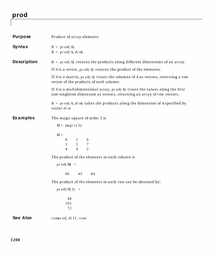
prod
1200
1prodPurpose Product of array elements
Syntax B = prod(A)B = prod(A,dim)
Description B = prod(A) returns the products along different dimensions of an array.
If A is a vector, prod(A) returns the product of the elements.
If A is a matrix, prod(A) treats the columns of A as vectors, returning a rowvector of the products of each column.
If A is a multidimensional array, prod(A) treats the values along the firstnon-singleton dimension as vectors, returning an array of row vectors.
B = prod(A,dim) takes the products along the dimension of A specified byscalar dim.
Examples The magic square of order 3 is
M = magic(3)
M =8 1 63 5 74 9 2
The product of the elements in each column is
prod(M) =
96 45 84
The product of the elements in each row can be obtained by:
prod(M,2) =
4810572
See Also cumprod, diff, sum
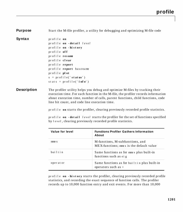
profile
1201
1profilePurpose Start the M-file profiler, a utility for debugging and optimizing M-file code
Syntax profile onprofile on -detail levelprofile on -historyprofile offprofile resumeprofile clearprofile reportprofile report basenameprofile plots = profile('status')stats = profile('info')
Description The profiler utility helps you debug and optimize M-files by tracking theirexecution time. For each function in the M-file, the profiler records informationabout execution time, number of calls, parent functions, child functions, codeline hit count, and code line execution time.
profile on starts the profiler, clearing previously recorded profile statistics.
profile on -detail level starts the profiler for the set of functions specifiedby level, clearing previously recorded profile statistics.
profile on -history starts the profiler, clearing previously recorded profilestatistics, and recording the exact sequence of function calls. The profilerrecords up to 10,000 function entry and exit events. For more than 10,000
Value for level Functions Profiler Gathers InformationAbout
mmex M-functions, M-subfunctions, andMEX-functions; mmex is the default value
builtin Same functions as for mmex plus built-infunctions such as eig
operator Same functions as for builtin plus built-inoperators such as +
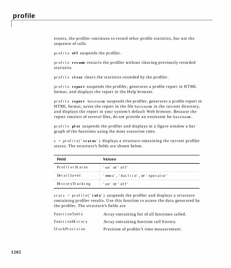
profile
1202
events, the profiler continues to record other profile statistics, but not thesequence of calls.
profile off suspends the profiler.
profile resume restarts the profiler without clearing previously recordedstatistics.
profile clear clears the statistics recorded by the profiler.
profile report suspends the profiler, generates a profile report in HTMLformat, and displays the report in the Help browser.
profile report basename suspends the profiler, generates a profile report inHTML format, saves the report in the file basename in the current directory,and displays the report in your system’s default Web browser. Because thereport consists of several files, do not provide an extension for basename.
profile plot suspends the profiler and displays in a figure window a bargraph of the functions using the most execution time.
s = profile('status') displays a structure containing the current profilerstatus. The structure’s fields are shown below.
stats = profile('info') suspends the profiler and displays a structurecontaining profiler results. Use this function to access the data generated bythe profiler. The structure’s fields are
Field Values
ProfilerStatus 'on' or 'off'
DetailLevel 'mmex', 'builtin', or 'operator'
HistoryTracking 'on' or 'off'
FunctionTable Array containing list of all functions called.
FunctionHistory Array containing function call history.
ClockPrecision Precision of profiler’s time measurement.
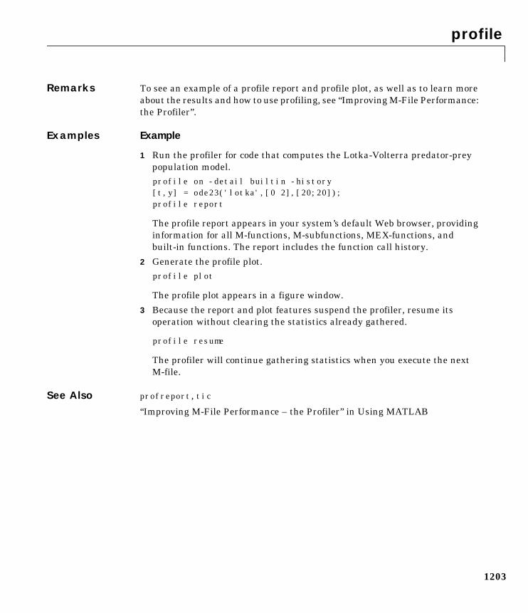
profile
1203
Remarks To see an example of a profile report and profile plot, as well as to learn moreabout the results and how to use profiling, see “Improving M-File Performance:the Profiler”.
Examples Example
1 Run the profiler for code that computes the Lotka-Volterra predator-preypopulation model.profile on -detail builtin -history[t,y] = ode23('lotka',[0 2],[20;20]);profile report
The profile report appears in your system’s default Web browser, providinginformation for all M-functions, M-subfunctions, MEX-functions, andbuilt-in functions. The report includes the function call history.
2 Generate the profile plot.profile plot
The profile plot appears in a figure window.
3 Because the report and plot features suspend the profiler, resume itsoperation without clearing the statistics already gathered.
profile resume
The profiler will continue gathering statistics when you execute the nextM-file.
See Also profreport, tic
“Improving M-File Performance – the Profiler” in Using MATLAB
profreport
1204
1profreportPurpose Generate a profile report
Syntax profreportprofreport(basename)profreport(stats)profreport(basename,stats)
Description profreport suspends the profiler, generates a profile report in HTML formatusing the current profiler results, and displays the report in a Web browser.
profreport(basename) suspends the profiler, generates a profile report inHTML format using the current profiler results, saves the report using thebasename you supply, and displays the report in a Web browser. Because thereport consists of several files, do not provide an extension for basename.
profreport(stats) suspends the profiler, generates a profile report in HTMLformat using the profiler results info, and displays the report in a Webbrowser. stats is the profiler information structure returned by stats =profile('info').
profreport(basename,stats) suspends the profiler, generates a profile reportin HTML format using the profiler results stats, saves the report using thebasename you supply, and displays the report in a Web browser. stats is theprofiler information structure returned by stats = profile('info'). Becausethe report consists of several files, do not provide an extension for basename.
Examples Run profiler and view the structure containing profile results.
1 Run the profiler for code that computes the Lotka-Volterra predator-preypopulation model.profile on -detail builtin -history[t,y] = ode23('lotka',[0 2],[20;20]);
2 View the structure containing the profile results.stats = profile('info')
MATLAB returnsstats =FunctionTable: [42x1 struct]
profreport
1205
FunctionHistory: [2x830 double] ClockPrecision: 0.0100 Name: 'MATLAB'
3 View the contents of the second element in the FunctionTable structure.stats.FunctionTable(2)
MATLAB returnsans = FunctionName: 'horzcat' FileName: '' Type: 'Builtin-function' NumCalls: 43 TotalTime: 0 TotalRecursiveTime: 0 Children: [0x1 struct] Parents: [2x1 struct] ExecutedLines: [0x3 double]
4 Display the profile report from the structure.
profreport(stats)
MATLAB displays the profile report in a Web browser.
See Also profile
“Improving M-File Performance: the Profiler” in Using MATLAB
propedit
1206
1propeditPurpose Starts the Property Editor
Syntax propeditpropedit(HandleList)
Description propedit starts the Property Editor, a graphical user interface to theproperties of Handle Graphics objects. If you call it without any inputarguments, the Property Editor displays the properties of the current figure, ifthere are more than one figure displayed, or the root object, if there is nocurrently active figure.
propedit(HandleList) edits the properties for the object (or objects) inHandleList.
Note Starting the Property Editor enables plot editing mode for the figure.
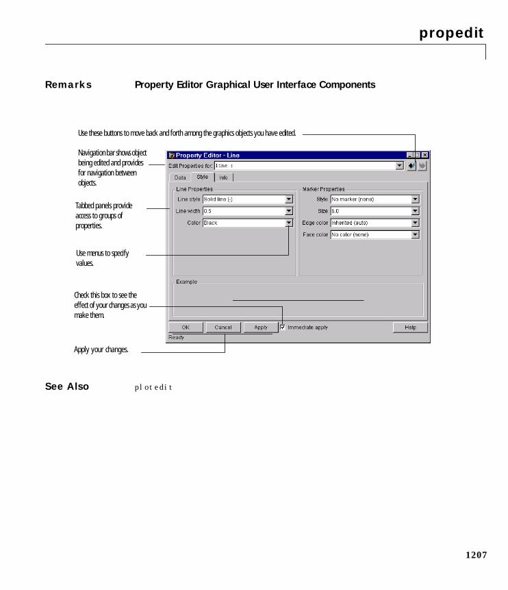
propedit
1207
Remarks Property Editor Graphical User Interface Components
See Also plotedit
Use these buttons to move back and forth among the graphics objects you have edited.
Use menus to specifyvalues.
Tabbed panels provideaccess to groups ofproperties.
Check this box to see theeffect of your changes as youmake them.
Apply your changes.
Navigation bar shows objectbeing edited and providesfor navigation betweenobjects.
pwd
1208
1pwdPurpose Display current directory
GraphicalInterface
As an alternative to the pwd function, use the Current Directory field in theMATLAB desktop toolbar.
Syntax pwds = pwd
Description pwd displays the current working directory.
s = pwd returns the current directory to the variable s.
See Also cd, dir, path, what
qmr
1209
1qmrPurpose Quasi-Minimal Residual method
Syntax x = qmr(A,b)qmr(A,b,tol)qmr(A,b,tol,maxit)qmr(A,b,tol,maxit,M)qmr(A,b,tol,maxit,M1,M2)qmr(A,b,tol,maxit,M1,M2,x0)qmr(afun,b,tol,maxit,m1fun,m2fun,x0,p1,p2,...)[x,flag] = qmr(A,b,...)[x,flag,relres] = qmr(A,b,...)[x,flag,relres,iter] = qmr(A,b,...)[x,flag,relres,iter,resvec] = qmr(A,b,...)
Description x = qmr(A,b) attempts to solve the system of linear equations A*x=b for x. Then-by-n coefficient matrix A must be square and the column vector b must havelength n. A can be a function afun such that afun(x) returns A*x andafun(x,'transp') returns A'*x.
If qmr converges, a message to that effect is displayed. If qmr fails to convergeafter the maximum number of iterations or halts for any reason, a warningmessage is printed displaying the relative residual norm(b-A*x)/norm(b) andthe iteration number at which the method stopped or failed.
qmr(A,b,tol) specifies the tolerance of the method. If tol is [], then qmr usesthe default, 1e-6.
qmr(A,b,tol,maxit) specifies the maximum number of iterations. If maxit is[], then qmr uses the default, min(n,20).
qmr(A,b,tol,maxit,M) and qmr(A,b,tol,maxit,M1,M2) use preconditionersM or M = M1*M2 and effectively solve the system inv(M)*A*x = inv(M)*b for x.If M is [] then qmr applies no preconditioner. M can be a function mfun such thatmfun(x) returns M\x and mfun(x,'transp') returns M'\x.
qmr(A,b,tol,maxit,M1,M2,x0) specifies the initial guess. If x0 is [], then qmruses the default, an all zero vector.
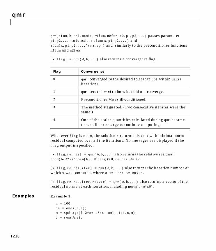
qmr
1210
qmr(afun,b,tol,maxit,m1fun,m2fun,x0,p1,p2,...) passes parametersp1,p2,... to functions afun(x,p1,p2,...) andafun(x,p1,p2,...,'transp') and similarly to the preconditioner functionsm1fun and m2fun.
[x,flag] = qmr(A,b,...) also returns a convergence flag.
Whenever flag is not 0, the solution x returned is that with minimal normresidual computed over all the iterations. No messages are displayed if theflag output is specified.
[x,flag,relres] = qmr(A,b,...) also returns the relative residualnorm(b-A*x)/norm(b). If flag is 0, relres <= tol.
[x,flag,relres,iter] = qmr(A,b,...) also returns the iteration number atwhich x was computed, where 0 <= iter <= maxit.
[x,flag,relres,iter,resvec] = qmr(A,b,...) also returns a vector of theresidual norms at each iteration, including norm(b-A*x0).
Examples Example 1.
n = 100;on = ones(n,1);A = spdiags([-2*on 4*on -on],-1:1,n,n);b = sum(A,2);
Flag Convergence
0 qmr converged to the desired tolerance tol within maxititerations.
1 qmr iterated maxit times but did not converge.
2 Preconditioner M was ill-conditioned.
3 The method stagnated. (Two consecutive iterates were thesame.)
4 One of the scalar quantities calculated during qmr becametoo small or too large to continue computing.
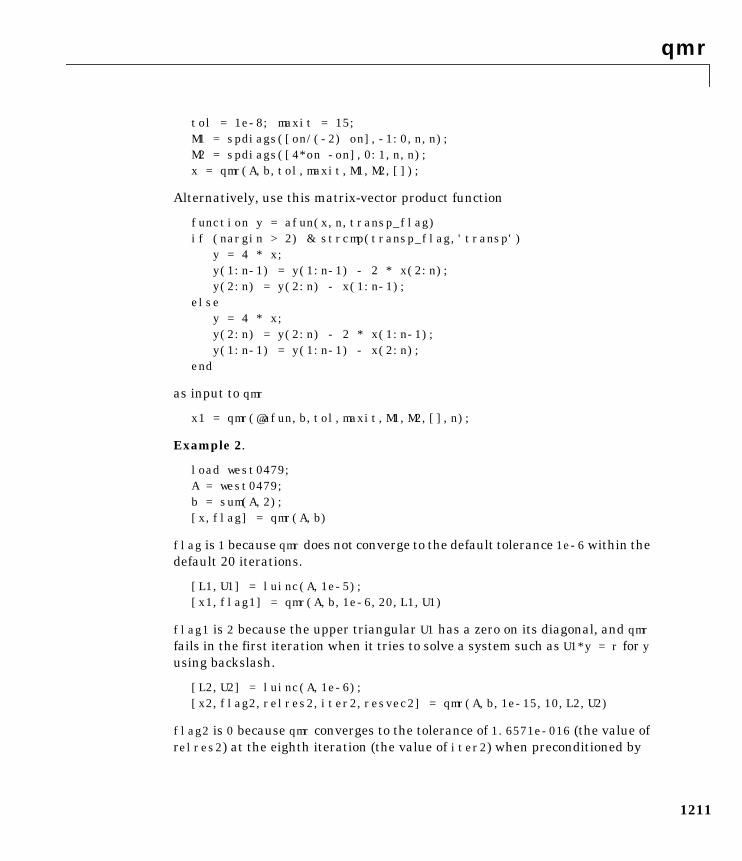
qmr
1211
tol = 1e-8; maxit = 15;M1 = spdiags([on/(-2) on],-1:0,n,n);M2 = spdiags([4*on -on],0:1,n,n);x = qmr(A,b,tol,maxit,M1,M2,[]);
Alternatively, use this matrix-vector product function
function y = afun(x,n,transp_flag)if (nargin > 2) & strcmp(transp_flag,'transp') y = 4 * x; y(1:n-1) = y(1:n-1) - 2 * x(2:n); y(2:n) = y(2:n) - x(1:n-1);else y = 4 * x; y(2:n) = y(2:n) - 2 * x(1:n-1); y(1:n-1) = y(1:n-1) - x(2:n);end
as input to qmr
x1 = qmr(@afun,b,tol,maxit,M1,M2,[],n);
Example 2.
load west0479;A = west0479;b = sum(A,2);[x,flag] = qmr(A,b)
flag is 1 because qmr does not converge to the default tolerance 1e-6 within thedefault 20 iterations.
[L1,U1] = luinc(A,1e-5);[x1,flag1] = qmr(A,b,1e-6,20,L1,U1)
flag1 is 2 because the upper triangular U1 has a zero on its diagonal, and qmrfails in the first iteration when it tries to solve a system such as U1*y = r for yusing backslash.
[L2,U2] = luinc(A,1e-6);[x2,flag2,relres2,iter2,resvec2] = qmr(A,b,1e-15,10,L2,U2)
flag2 is 0 because qmr converges to the tolerance of 1.6571e-016 (the value ofrelres2) at the eighth iteration (the value of iter2) when preconditioned by
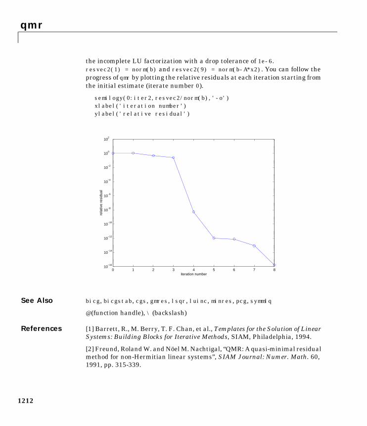
qmr
1212
the incomplete LU factorization with a drop tolerance of 1e-6.resvec2(1) = norm(b) and resvec2(9) = norm(b-A*x2). You can follow theprogress of qmr by plotting the relative residuals at each iteration starting fromthe initial estimate (iterate number 0).
semilogy(0:iter2,resvec2/norm(b),'-o')xlabel('iteration number’)ylabel('relative residual')
See Also bicg, bicgstab, cgs, gmres, lsqr, luinc, minres, pcg, symmlq
@ (function handle), \ (backslash)
References [1] Barrett, R., M. Berry, T. F. Chan, et al., Templates for the Solution of LinearSystems: Building Blocks for Iterative Methods, SIAM, Philadelphia, 1994.
[2] Freund, Roland W. and Nöel M. Nachtigal, “QMR: A quasi-minimal residualmethod for non-Hermitian linear systems”, SIAM Journal: Numer. Math. 60,1991, pp. 315-339.
0 1 2 3 4 5 6 7 810
−16
10−14
10−12
10−10
10−8
10−6
10−4
10−2
100
102
iteration number
rela
tive
resi
dual
qr
1213
1qrPurpose Orthogonal-triangular decomposition
Syntax [Q,R] = qr(A)[Q,R,E] = qr(A)[Q,R] = qr(A,0)[Q,R,E] = qr(A,0)R = qr(A) (sparse matrices)[C,R] = qr(A,B) (sparse matrices)R = qr(A,0) (sparse matrices)[C,R] = qr(A,B,0) (sparse matrices)X = qr(A)
Description The qr function performs the orthogonal-triangular decomposition of a matrix.This factorization is useful for both square and rectangular matrices. Itexpresses the matrix as the product of a real orthonormal or complex unitarymatrix and an upper triangular matrix.
[Q,R] = qr(A) produces an upper triangular matrix R of the same dimensionas A and a unitary matrix Q so that A = Q∗R. For sparse matrices, Q is oftennearly full.
[Q,R,E] = qr(A) produces a permutation matrix E, an upper triangularmatrix R with decreasing diagonal elements, and a unitary matrix Q so thatA∗E = Q∗R. The column permutation E is chosen so that abs(diag(R)) isdecreasing.
[Q,R] = qr(A,0) and [Q,R,E] = qr(A,0) produce “economy-size”decompositions in which E is a permutation vector, so that Q*R = A(:,E). Thecolumn permutation E is chosen so that abs(diag(R)) is decreasing.
R = qr(A) for sparse matrices, produces only an upper triangular matrix, R.The matrix R provides a Cholesky factorization for the matrix associated withthe normal equations,
R'*R = A'*A
This approach avoids the loss of numerical information inherent in thecomputation of A'*A.
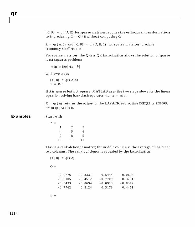
qr
1214
[C,R] = qr(A,B) for sparse matrices, applies the orthogonal transformationsto B, producing C = Q'*B without computing Q.
R = qr(A,0) and [C,R] = qr(A,B,0) for sparse matrices, produce“economy-size” results.
For sparse matrices, the Q-less QR factorization allows the solution of sparseleast squares problems
with two steps
[C,R] = qr(A,b)x = R\c
If A is sparse but not square, MATLAB uses the two steps above for the linearequation solving backslash operator, i.e., x = A\b.
X = qr(A) returns the output of the LAPACK subroutine DGEQRF or ZGEQRF.triu(qr(A)) is R.
Examples Start with
A =1 2 34 5 67 8 9
10 11 12
This is a rank-deficient matrix; the middle column is the average of the othertwo columns. The rank deficiency is revealed by the factorization:
[Q,R] = qr(A)
Q =
-0.0776 -0.8331 0.5444 0.0605-0.3105 -0.4512 -0.7709 0.3251-0.5433 -0.0694 -0.0913 -0.8317-0.7762 0.3124 0.3178 0.4461
R =
minimize Ax b–
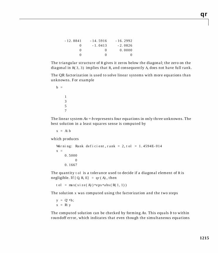
qr
1215
-12.8841 -14.5916 -16.29920 -1.0413 -2.08260 0 0.00000 0 0
The triangular structure of R gives it zeros below the diagonal; the zero on thediagonal in R(3,3) implies that R, and consequently A, does not have full rank.
The QR factorization is used to solve linear systems with more equations thanunknowns. For example
b =
1357
The linear system Ax = brepresents four equations in only three unknowns. Thebest solution in a least squares sense is computed by
x = A\b
which produces
Warning: Rank deficient, rank = 2, tol = 1.4594E-014x =
0.50000
0.1667
The quantity tol is a tolerance used to decide if a diagonal element of R isnegligible. If [Q,R,E] = qr(A), then
tol = max(size(A))∗eps∗abs(R(1,1))
The solution x was computed using the factorization and the two steps
y = Q'∗b;x = R\y
The computed solution can be checked by forming Ax. This equals b to withinroundoff error, which indicates that even though the simultaneous equations
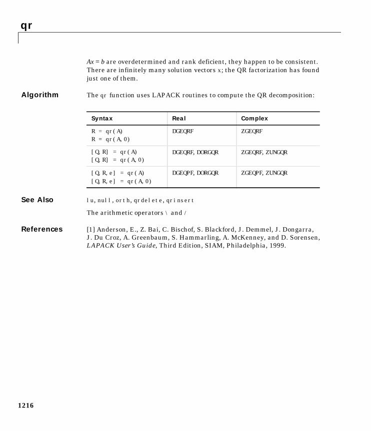
qr
1216
Ax= b are overdetermined and rank deficient, they happen to be consistent.There are infinitely many solution vectors x; the QR factorization has foundjust one of them.
Algorithm The qr function uses LAPACK routines to compute the QR decomposition:
See Also lu, null, orth, qrdelete, qrinsert
The arithmetic operators \ and /
References [1] Anderson, E., Z. Bai, C. Bischof, S. Blackford, J. Demmel, J. Dongarra,J. Du Croz, A. Greenbaum, S. Hammarling, A. McKenney, and D. Sorensen,LAPACK User’s Guide, Third Edition, SIAM, Philadelphia, 1999.
Syntax Real Complex
R = qr(A)R = qr(A,0)
DGEQRF ZGEQRF
[Q,R] = qr(A)[Q,R] = qr(A,0)
DGEQRF, DORGQR ZGEQRF, ZUNGQR
[Q,R,e] = qr(A)[Q,R,e] = qr(A,0)
DGEQPF, DORGQR ZGEQPF, ZUNGQR
qrdelete
1217
1qrdeletePurpose Delete column from QR factorization
Syntax [Q,R] = qrdelete(Q,R,j)
Description [Q,R] = qrdelete(Q,R,j) changes Q and R to be the factorization of thematrix A with its jth column, A(:,j), removed.
Inputs Q and R represent the original QR factorization of matrix A, as returnedby the statement [Q,R] = qr(A). Argument j specifies the column to beremoved from matrix A.
Algorithm The qrdelete function uses a series of Givens rotations to zero out theappropriate elements of the factorization.
See Also qr, qrinsert
qrinsert
1218
1qrinsertPurpose Insert column in QR factorization
Syntax [Q,R] = qrinsert(Q,R,j,x)
Description [Q,R] = qrinsert(Q,R,j,x) changes Q and R to be the factorization of thematrix obtained by inserting an extra column, x, before A(:,j). If A has ncolumns and j = n+1, then qrinsert inserts x after the last column of A.
Inputs Q and R represent the original QR factorization of matrix A, as returnedby the statement [Q,R] = qr(A). Argument x is the column vector to beinserted into matrix A. Argument j specifies the column before which x isinserted.
Algorithm The qrinsert function inserts the values of x into the jth column of R. It thenuses a series of Givens rotations to zero out the nonzero elements of R on andbelow the diagonal in the jth column.
See Also qr, qrdelete
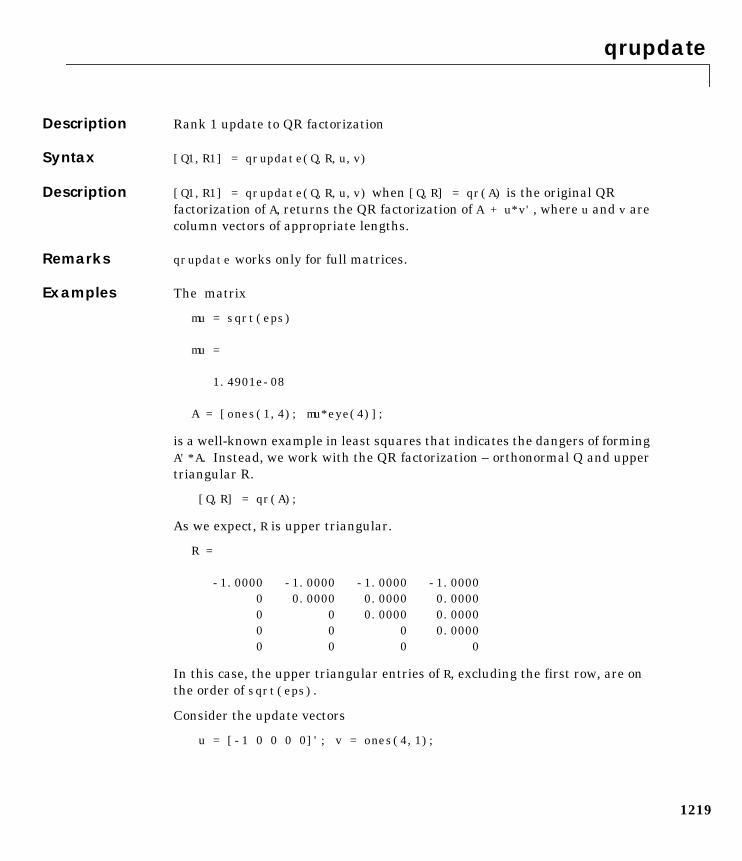
qrupdate
1219
1qrupdateDescription Rank 1 update to QR factorization
Syntax [Q1,R1] = qrupdate(Q,R,u,v)
Description [Q1,R1] = qrupdate(Q,R,u,v) when [Q,R] = qr(A) is the original QRfactorization of A, returns the QR factorization of A + u*v', where u and v arecolumn vectors of appropriate lengths.
Remarks qrupdate works only for full matrices.
Examples The matrix
mu = sqrt(eps)
mu =
1.4901e-08
A = [ones(1,4); mu*eye(4)];
is a well-known example in least squares that indicates the dangers of formingA'*A. Instead, we work with the QR factorization – orthonormal Q and uppertriangular R.
[Q,R] = qr(A);
As we expect, R is upper triangular.
R =
-1.0000 -1.0000 -1.0000 -1.0000 0 0.0000 0.0000 0.0000 0 0 0.0000 0.0000 0 0 0 0.0000 0 0 0 0
In this case, the upper triangular entries of R, excluding the first row, are onthe order of sqrt(eps).
Consider the update vectors
u = [-1 0 0 0 0]'; v = ones(4,1);
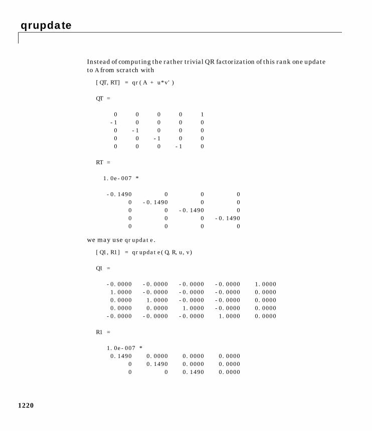
qrupdate
1220
Instead of computing the rather trivial QR factorization of this rank one updateto A from scratch with
[QT,RT] = qr(A + u*v')
QT =
0 0 0 0 1 -1 0 0 0 0 0 -1 0 0 0 0 0 -1 0 0 0 0 0 -1 0
RT =
1.0e-007 *
-0.1490 0 0 0 0 -0.1490 0 0 0 0 -0.1490 0 0 0 0 -0.1490 0 0 0 0
we may use qrupdate.
[Q1,R1] = qrupdate(Q,R,u,v)
Q1 =
-0.0000 -0.0000 -0.0000 -0.0000 1.0000 1.0000 -0.0000 -0.0000 -0.0000 0.0000 0.0000 1.0000 -0.0000 -0.0000 0.0000 0.0000 0.0000 1.0000 -0.0000 0.0000 -0.0000 -0.0000 -0.0000 1.0000 0.0000
R1 =
1.0e-007 * 0.1490 0.0000 0.0000 0.0000 0 0.1490 0.0000 0.0000 0 0 0.1490 0.0000
qrupdate
1221
0 0 0 0.1490 0 0 0 0
Note that both factorizations are correct, even though they are different.
Algorithm qrupdate uses the algorithm in section 12.5.1 of the third edition of MatrixComputations by Golub and van Loan. qrupdate is useful since, if we takeN = max(m,n), then computing the new QR factorization from scratch isroughly an algorithm, while simply updating the existing factors in thisway is an algorithm.
References Golub, Gene H. and Charles Van Loan, Matrix Computations, Third Edition,Johns Hopkins University Press, Baltimore, 1996
See Also cholupdate, qr
O N3( )O N2( )
quad, quad8
1222
1quad, quad8Purpose Numerically evaluate integral, adaptive Simpson quadrature
Note The quad8 function, which implemented a higher order method, isobsolete. The quadl function is its recommended replacement.
Syntax q = quad(fun,a,b)q = quad(fun,a,b,tol)q = quad(fun,a,b,tol,trace)q = quad(fun,a,b,tol,trace,p1,p2,...)[q,fcnt] = quadl(fun,a,b,...)
Description Quadrature is a numerical method used to find the area under the graph of afunction, that is, to compute a definite integral.
q = quad(fun,a,b) approximates the integral of function fun from a to b towithin an error of 10-6 using recursive adaptive Simpson quadrature. funaccepts a vector x and returns a vector y, the function fun evaluated at eachelement of x.
q = quad(fun,a,b,tol) uses an absolute error tolerance tol instead of thedefault which is 1.0e-6. Larger values of tol result in fewer functionevaluations and faster computation, but less accurate results. In MATLABversion 5.3 and earlier, the quad function used a less reliable algorithm and adefault relative tolerance of 1.0e-3.
q = quad(fun,a,b,tol,trace) with non-zero trace shows the values of[fcnt a b-a Q] during the recursion.
q = quad(fun,a,b,tol,trace,p1,p2,...) provides for additional argumentsp1,p2,... to be passed directly to function fun, fun(x,p1,p2,...). Passempty matrices for tol or trace to use the default values.
[q,fcnt] = quad(...) returns the number of function evaluations.
q f x( ) xda
b
∫=
quad, quad8
1223
The function quadl may be more efficient with high accuracies and smoothintegrands.
Examples You can specify fun three different ways:
• A string expression involving a single variableQ = quad('1./(x.^3-2*x-5)',0,2);
• An inline objectF = inline('1./(x.^3-2*x-5)');Q = quad(F,0,2);
• A function handleQ = quad(@myfun,0,2);
where myfun.m is an M-file.function y = myfun(x)y = 1./(x.^3-2*x-5);
Algorithm quad implements a low order method using an adaptive recursive Simpson’srule.
Diagnostics quad may issue one of the following warnings:
'Minimum step size reached' indicates that the recursive intervalsubdivision has produced a subinterval whose length is on the order of roundofferror in the length of the original interval. A nonintegrable singularity ispossible.
'Maximum function count exceeded' indicates that the integrand has beenevaluated more than 10,000 times. A nonintegrable singularity is likely.
'Infinite or Not-a-Number function value encountered' indicates afloating point overflow or division by zero during the evaluation of theintegrand in the interior of the interval.
See Also dblquad, inline, quadl, @ (function handle)
quad, quad8
1224
References [1] Gander, W. and W. Gautschi, “Adaptive Quadrature – Revisited”, BIT, Vol.40, 2000, pp. 84-101. This document is also available athttp://www.inf.ethz.ch/personal/gander.
quadl
1225
1quadlPurpose Numerically evaluate integral, adaptive Lobatto quadrature
Syntax q = quadl(fun,a,b)q = quadl(fun,a,b,tol)q = quadl(fun,a,b,tol,trace)q = quadl(fun,a,b,tol,trace,p1,p2,...)[q,fcnt] = quadl(fun,a,b,...)
Description q = quadl(fun,a,b) approximates the integral of function fun from a to b, towithin an error of 10-6 using recursive adaptive Lobatto quadrature. funaccepts a vector x and returns a vector y, the function fun evaluated at eachelement of x.
q = quadl(fun,a,b,tol) uses an absolute error tolerance of tol instead of thedefault, which is 1.0e-6. Larger values of tol result in fewer functionevaluations and faster computation, but less accurate results.
quadl(fun,a,b,tol,trace) with non-zero trace shows the values of[fcnt a b-a q] during the recursion.
quadl(fun,a,b,tol,trace,p1,p2,...) provides for additional argumentsp1,p2,... to be passed directly to function fun, fun(x,p1,p2,...). Passempty matrices for tol or trace to use the default values.
[q,fcnt] = quadl(...) returns the number of function evaluations.
Use array operators .*, ./ and .^ in the definition of fun so that it can beevaluated with a vector argument.
The function quad may be more efficient with low accuracies or nonsmoothintegrands.
Examples You can specify fun three different ways:
• A string expression involving a single variableQ = quadl('1./(x.^3-2*x-5)',0,2);
• An inline objectF = inline('1./(x.^3-2*x-5)');Q = quadl(F,0,2);
quadl
1226
• A function handleQ = quadl(@myfun,0,2);
where myfun.m is an M-file.function y = myfun(x)y = 1./(x.^3-2*x-5);
Algorithm quadl implements a high order method using an adaptive Gauss/Lobattoqudrature rule.
Diagnostics quadl may issue one of the following warnings:
'Minimum step size reached' indicates that the recursive intervalsubdivision has produced a subinterval whose length is on the order of roundofferror in the length of the original interval. A nonintegrable singularity ispossible.
'Maximum function count exceeded' indicates that the integrand has beenevaluated more than 10,000 times. A nonintegrable singularity is likely.
'Infinite or Not-a-Number function value encountered' indicates afloating point overflow or division by zero during the evaluation of theintegrand in the interior of the interval.
See Also dblquad, inline, quad, @ (function handle)
References [1] Gander, W. and W. Gautschi, “Adaptive Quadrature – Revisited”, BIT,Vol. 40, 2000, pp. 84-101. This document is also available athttp://www.inf.ethz.ch/personal/gander.
questdlg
1227
1questdlgPurpose Create and display question dialog box
Syntax button = questdlg('qstring')button = questdlg('qstring','title')button = questdlg('qstring','title','default')button = questdlg('qstring','title','str1','str2','default')button = questdlg('qstring','title','str1','str2','str3','default')
Description button = questdlg('qstring') displays a modal dialog presenting thequestion 'qstring'. The dialog has three default buttons, Yes, No, andCancel. 'qstring' is a cell array or a string that automatically wraps to fitwithin the dialog box. button contains the name of the button pressed.
button = questdlg('qstring','title') displays a question dialog with'title' displayed in the dialog’s title bar.
button = questdlg('qstring','title','default') specifies which pushbutton is the default in the event that the Return key is pressed. 'default'must be 'Yes', 'No', or 'Cancel'.
button = questdlg('qstring','title','str1','str2','default') createsa question dialog box with two push buttons labeled 'str1' and 'str2'.'default' specifies the default button selection and must be 'str1' or 'str2'.
button =questdlg('qstring','title','str1','str2','str3','default') creates aquestion dialog box with three push buttons labeled 'str1', 'str2', and'str3'. 'default' specifies the default button selection and must be 'str1','str2', or 'str3'.
Example Create a question dialog asking the user whether to continue a hypotheticaloperation:
button = questdlg('Do you want to continue?',...'Continue Operation','Yes','No','Help','No');if strcmp(button,'Yes')
disp('Creating file')elseif strcmp(button,'No')
disp('Canceled file operation')
questdlg
1228
elseif strcmp(button,'Help')disp('Sorry, no help available')
end
See Also dialog, errordlg, helpdlg, inputdlg, msgbox, warndlg
quit
1229
1quitPurpose Terminate MATLAB
GraphicalInterface
As an alternative to the quit function, use the close box or select Exit MATLABfrom the File menu in the MATLAB desktop.
Syntax quitquit cancelquit force
Description quit terminates MATLAB after running finish.m, if finish.m exists. Theworkspace is not automatically saved by quit. To save the workspace orperform other actions when quitting, create a finish.m file to perform thoseactions. If an error occurs while finish.m is running, quit is canceled so thatyou can correct your finish.m file without losing your workspace.
quit cancel is for use in finish.m and cancels quitting. It has no effectanywhere else.
quit force bypasses finish.m and terminates MATLAB. Use this to overridefinish.m, for example, if an errant finish.m will not let you quit.
Remarks When using Handle Graphics in finish.m, use uiwait, waitfor, or drawnow sothat figures are visible. See the reference pages for these functions for moreinformation.
Examples Two sample finish.m files are included with MATLAB. Use them to help youcreate your own finish.m, or rename one of the files to finish.m to use it.
• finishsav.m – saves the workspace to a MAT-file when MATLAB quits
• finishdlg.m – displays a dialog allowing you to cancel quitting; it uses quitcancel and contains the following code.
button = questdlg('Ready to quit?', ... 'Exit Dialog','Yes','No','No');switch button case 'Yes', disp('Exiting MATLAB'); %Save variables to matlab.mat save
quit
1230
case 'No', quit cancel;end
See Also finish, save, startup
quiver
1231
1quiverPurpose Quiver or velocity plot
Syntax quiver(U,V)quiver(X,Y,U,V)quiver(...,scale)quiver(...,LineSpec)quiver(...,LineSpec,'filled')h = quiver(...)
Description A quiver plot displays vectors with components (u,v) at the points (x,y).
quiver(U,V) draws vectors specified by U and V at the coordinates defined byx = 1:n and y = 1:m, where [m,n] = size(U) = size(V). This syntax plots Uand V over a geometrically rectangular grid. quiver automatically scales thevectors based on the distance between them to prevent them from overlapping.
quiver(X,Y,U,V) draws vectors at each pair of elements in X and Y. If X and Yare vectors, length(X) = n and length(Y) = m, where[m,n] = size(U) = size(V). The vector X corresponds to the columns of U andV, and vector Y corresponds to the rows of U and V.
quiver(...,scale) automatically scales the vectors to prevent them fromoverlapping, then multiplies them by scale. scale = 2 doubles their relativelength and scale = 0.5 halves them. Use scale = 0 to plot the velocity vectorswithout the automatic scaling.
quiver(...,LineSpec) specifies line style, marker symbol, and color using anyvalid LineSpec. quiver draws the markers at the origin of the vectors.
quiver(...,LineSpec,'filled') fills markers specified by LineSpec.
h = quiver(...) returns a vector of line handles.
Remarks If X and Y are vectors, this function behaves as
[X,Y] = meshgrid(x,y)quiver(X,Y,U,V)
Examples Plot the gradient field of the function .z xe x2 y2––( )=
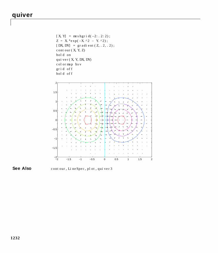
quiver
1232
[X,Y] = meshgrid(–2:.2:2);Z = X.∗exp(–X.^2 – Y.^2);[DX,DY] = gradient(Z,.2,.2);contour(X,Y,Z)hold onquiver(X,Y,DX,DY)colormap hsvgrid offhold off
See Also contour, LineSpec, plot, quiver3
−2 −1.5 −1 −0.5 0 0.5 1 1.5 2−2
−1.5
−1
−0.5
0
0.5
1
1.5
2
quiver3
1233
1quiver3Purpose Three-dimensional velocity plot
Syntax quiver3(Z,U,V,W)quiver3(X,Y,Z,U,V,W)quiver3(...,scale)quiver3(...,LineSpec)quiver3(...,LineSpec,'filled')h = quiver3(...)
Description A three-dimensional quiver plot displays vectors with components (u,v,w) atthe points (x,y,z).
quiver3(Z,U,V,W) plots the vectors at the equally spaced surface pointsspecified by matrix Z. quiver3 automatically scales the vectors based on thedistance between them to prevent them from overlapping.
quiver3(X,Y,Z,U,V,W) plots vectors with components (u,v,w) at the points(x,y,z). The matrices X, Y, Z, U, V, W must all be the same size and contain thecorresponding position and vector components.
quiver3(...,scale) automatically scales the vectors to prevent them fromoverlapping, then multiplies them by scale. scale = 2 doubles their relativelength and scale = 0.5 halves them. Use scale = 0 to plot the vectors withoutthe automatic scaling.
quiver3(...,LineSpec) specify line type and color using any valid LineSpec.
quiver3(...,LineSpec,'filled') fills markers specified by LineSpec.
h = quiver3(...) returns a vector of line handles.
Examples Plot the surface normals of the function .
[X,Y] = meshgrid(–2:0.25:2,–1:0.2:1);Z = X.* exp(–X.^2 – Y.^2);[U,V,W] = surfnorm(X,Y,Z);quiver3(X,Y,Z,U,V,W,0.5);hold onsurf(X,Y,Z);colormap hsv
z xe x2 y2––( )=
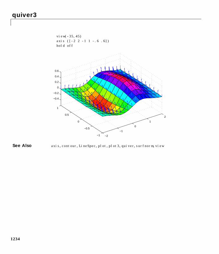
quiver3
1234
view(-35,45)axis ([-2 2 -1 1 -.6 .6])hold off
See Also axis, contour, LineSpec, plot, plot3, quiver, surfnorm, view
−2
−1
0
1
2
−1
−0.5
0
0.5
1
−0.4
−0.2
0
0.2
0.4
0.6
qz
1235
1qzPurpose QZ factorization for generalized eigenvalues
Syntax [AA,BB,Q,Z,V] = qz(A,B)[AA,BB,Q,Z,V] = qz(A,B,flag)
Description The qz function gives access to intermediate results in the computation ofgeneralized eigenvalues.
[AA,BB,Q,Z,V] = qz(A,B) for square matrices A and B, produces uppertriangular matrices AA and BB, unitary matrices Q and Z containing theproducts of the left and right transformations, such that Q*A*Z = AA, andQ*B*Z = BB, and the generalized eigenvector matrix V.
[AA,BB,Q,Z,V] = qz(A,B,flag) for real matrices A and B, produces one of twodecompositions depending on the value of flag:
If AA is triangular, the alphas and betas comprising the generalized eigenvaluesare the diagonal elements of AA and BB so that
A*V*diag(BB) = B*V*diag(AA)
If AA is quaditriangular, it is necessary to solve 2-by-2 generalized problems toobtain the actual eigenvalues.
For complex matrices A and B, AA and BB are always triangular.
Algorithm For real QZ on real A and real B, eig uses the LAPACK DGGES routine. If yourequest the fifth output V, eig also uses DTGEVC.
For complex QZ on real or complex A and B, eig uses the LAPACK ZGGESroutine. If you request the fifth output V, eig also uses ZTGEVC.
See Also eig
'complex' Produces a possibly complex decomposition with a triangularAA. 'complex' is the default.
'real' Produces a real decomposition with a quasitriangular AA,containing 1-by-1 and 2-by-2 blocks on its diagonal.
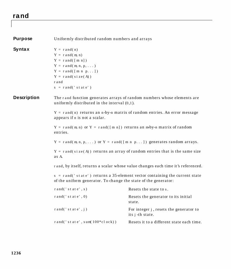
rand
1236
1randPurpose Uniformly distributed random numbers and arrays
Syntax Y = rand(n)Y = rand(m,n)Y = rand([m n])Y = rand(m,n,p,...)Y = rand([m n p...])Y = rand(size(A))rands = rand('state')
Description The rand function generates arrays of random numbers whose elements areuniformly distributed in the interval (0,1).
Y = rand(n) returns an n-by-n matrix of random entries. An error messageappears if n is not a scalar.
Y = rand(m,n) or Y = rand([m n]) returns an m-by-n matrix of randomentries.
Y = rand(m,n,p,...) or Y = rand([m n p...]) generates random arrays.
Y = rand(size(A)) returns an array of random entries that is the same sizeas A.
rand, by itself, returns a scalar whose value changes each time it’s referenced.
s = rand('state') returns a 35-element vector containing the current stateof the uniform generator. To change the state of the generator:
rand('state',s) Resets the state to s.
rand('state',0) Resets the generator to its initialstate.
rand('state',j) For integer j, resets the generator toits j-th state.
rand('state',sum(100*clock)) Resets it to a different state each time.
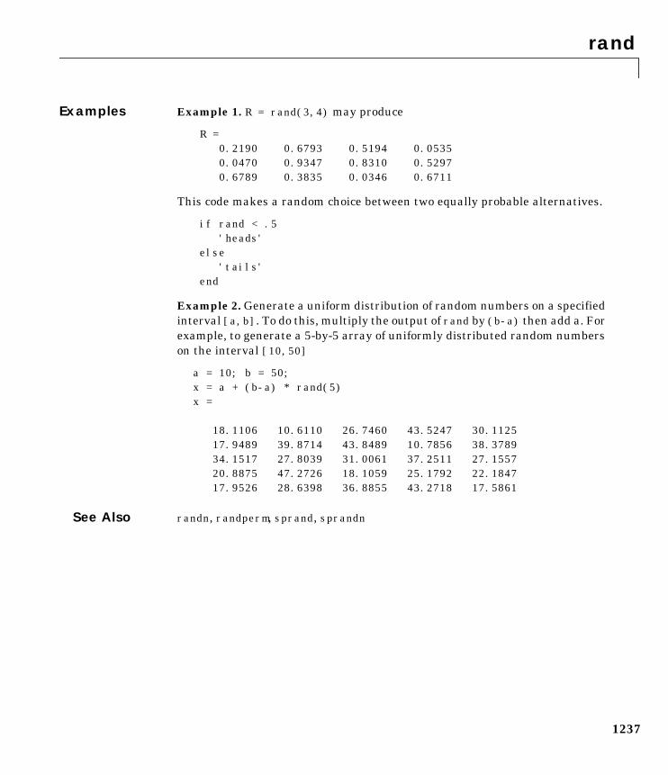
rand
1237
Examples Example 1. R = rand(3,4) may produce
R = 0.2190 0.6793 0.5194 0.0535 0.0470 0.9347 0.8310 0.5297 0.6789 0.3835 0.0346 0.6711
This code makes a random choice between two equally probable alternatives.
if rand < .5 'heads' else 'tails' end
Example 2. Generate a uniform distribution of random numbers on a specifiedinterval [a,b]. To do this, multiply the output of rand by (b-a) then add a. Forexample, to generate a 5-by-5 array of uniformly distributed random numberson the interval [10,50]
a = 10; b = 50;x = a + (b-a) * rand(5)x =
18.1106 10.6110 26.7460 43.5247 30.1125 17.9489 39.8714 43.8489 10.7856 38.3789 34.1517 27.8039 31.0061 37.2511 27.1557 20.8875 47.2726 18.1059 25.1792 22.1847 17.9526 28.6398 36.8855 43.2718 17.5861
See Also randn, randperm, sprand, sprandn
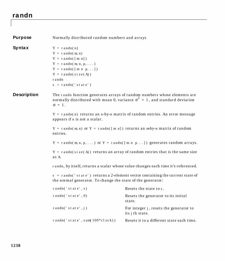
randn
1238
1randnPurpose Normally distributed random numbers and arrays
Syntax Y = randn(n)Y = randn(m,n)Y = randn([m n])Y = randn(m,n,p,...)Y = randn([m n p...])Y = randn(size(A))randns = randn('state')
Description The randn function generates arrays of random numbers whose elements arenormally distributed with mean 0, variance , and standard deviation
.
Y = randn(n) returns an n-by-n matrix of random entries. An error messageappears if n is not a scalar.
Y = randn(m,n) or Y = randn([m n]) returns an m-by-n matrix of randomentries.
Y = randn(m,n,p,...) or Y = randn([m n p...]) generates random arrays.
Y = randn(size(A)) returns an array of random entries that is the same sizeas A.
randn, by itself, returns a scalar whose value changes each time it’s referenced.
s = randn('state') returns a 2-element vector containing the current state ofthe normal generator. To change the state of the generator:
randn('state',s) Resets the state to s.
randn('state',0) Resets the generator to its initialstate.
randn('state',j) For integer j, resets the generator toits jth state.
randn('state',sum(100*clock)) Resets it to a different state each time.
σ2 1=σ 1=
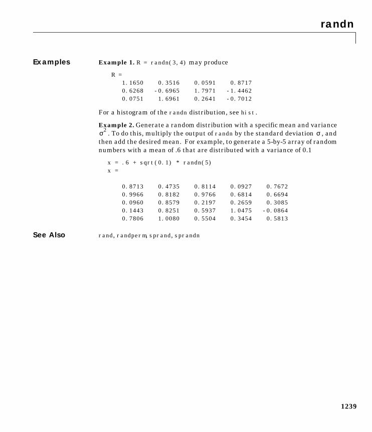
randn
1239
Examples Example 1. R = randn(3,4) may produce
R = 1.1650 0.3516 0.0591 0.8717 0.6268 -0.6965 1.7971 -1.4462 0.0751 1.6961 0.2641 -0.7012
For a histogram of the randn distribution, see hist.
Example 2. Generate a random distribution with a specific mean and variance. To do this, multiply the output of randn by the standard deviation , and
then add the desired mean. For example, to generate a 5-by-5 array of randomnumbers with a mean of .6 that are distributed with a variance of 0.1
x = .6 + sqrt(0.1) * randn(5)x =
0.8713 0.4735 0.8114 0.0927 0.7672 0.9966 0.8182 0.9766 0.6814 0.6694 0.0960 0.8579 0.2197 0.2659 0.3085 0.1443 0.8251 0.5937 1.0475 -0.0864 0.7806 1.0080 0.5504 0.3454 0.5813
See Also rand, randperm, sprand, sprandn
σ2 σ
randperm
1240
1randpermPurpose Random permutation
Syntax p = randperm(n)
Description p = randperm(n) returns a random permutation of the integers 1:n.
Remarks The randperm function calls rand and therefore changes rand’s state.
Examples randperm(6) might be the vector
[3 2 6 4 1 5]
or it might be some other permutation of 1:6.
See Also permute
rank
1241
1rankPurpose Rank of a matrix
Syntax k = rank(A)k = rank(A,tol)
Description The rank function provides an estimate of the number of linearly independentrows or columns of a matrix.
k = rank(A) returns the number of singular values of A that are larger thanthe default tolerance, max(size(A))∗norm(A)∗eps.
k = rank(A,tol) returns the number of singular values of A that are largerthan tol.
Algorithm There are a number of ways to compute the rank of a matrix. MATLAB usesthe method based on the singular value decomposition, or SVD. The SVDalgorithm is the most time consuming, but also the most reliable.
The rank algorithm is
s = svd(A);tol = max(size(A))∗s(1)∗eps;r = sum(s > tol);
References [1] Anderson, E., Z. Bai, C. Bischof, S. Blackford, J. Demmel, J. Dongarra,J. Du Croz, A. Greenbaum, S. Hammarling, A. McKenney, and D. Sorensen,LAPACK User’s Guide, Third Edition, SIAM, Philadelphia, 1999.
rat, rats
1242
1rat, ratsPurpose Rational fraction approximation
Syntax [N,D] = rat(X)[N,D] = rat(X,tol)rat(...)S = rats(X,strlen)S = rats(X)
Description Even though all floating-point numbers are rational numbers, it is sometimesdesirable to approximate them by simple rational numbers, which are fractionswhose numerator and denominator are small integers. The rat functionattempts to do this. Rational approximations are generated by truncatingcontinued fraction expansions. The rats function calls rat, and returns strings.
[N,D] = rat(X) returns arrays N and D so that N./D approximates X to withinthe default tolerance, 1.e-6*norm(X(:),1).
[N,D] = rat(X,tol) returns N./D approximating X to within tol.
rat(X), with no output arguments, simply displays the continued fraction.
S = rats(X,strlen) returns a string containing simple rationalapproximations to the elements of X. Asterisks are used for elements thatcannot be printed in the allotted space, but are not negligible compared to theother elements in X. strlen is the length of each string element returned by therats function. The default is strlen = 13, which allows 6 elements in 78spaces.
S = rats(X) returns the same results as those printed by MATLAB withformat rat.
Examples Ordinarily, the statement
s = 1 - 1/2 + 1/3 - 1/4 + 1/5 - 1/6 + 1/7
produces
s = 0.7595
rat, rats
1243
However, with
format rat
or with
rats(s)
the printed result is
s = 319/420
This is a simple rational number. Its denominator is 420, the least commonmultiple of the denominators of the terms involved in the original expression.Even though the quantity s is stored internally as a binary floating-pointnumber, the desired rational form can be reconstructed.
To see how the rational approximation is generated, the statement rat(s)
produces
1 + 1/(-4 + 1/(-6 + 1/(-3 + 1/(-5))))
And the statement
[n,d] = rat(s)
produces
n = 319, d = 420
The mathematical quantity π is certainly not a rational number, but theMATLAB quantity pi that approximates it is a rational number. pi is the ratioof a large integer and 252:
14148475504056880/4503599627370496
However, this is not a simple rational number. The value printed for pi withformat rat, or with rats(pi), is
355/113
This approximation was known in Euclid’s time. Its decimal representation is
3.14159292035398
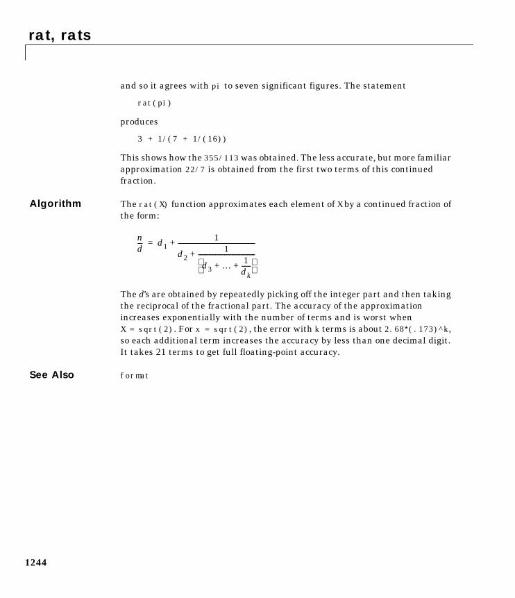
rat, rats
1244
and so it agrees with pi to seven significant figures. The statement
rat(pi)
produces
3 + 1/(7 + 1/(16))
This shows how the 355/113was obtained. The less accurate, but more familiarapproximation 22/7 is obtained from the first two terms of this continuedfraction.
Algorithm The rat(X) function approximates each element of X by a continued fraction ofthe form:
The d’s are obtained by repeatedly picking off the integer part and then takingthe reciprocal of the fractional part. The accuracy of the approximationincreases exponentially with the number of terms and is worst whenX = sqrt(2). For x = sqrt(2), the error with k terms is about 2.68∗(.173)^k,so each additional term increases the accuracy by less than one decimal digit.It takes 21 terms to get full floating-point accuracy.
See Also format
nd--- d1
1
d21
d3 … 1dk------+ +
-------------------------------------+
--------------------------------------------------+=
rbbox
1245
1rbboxPurpose Create rubberband box for area selection
Synopsis rbboxrbbox(initialRect)rbbox(initialRect,fixedPoint)rbbox(initialRect,fixedPoint,stepSize)finalRect = rbbox(...)
Description rbbox initializes and tracks a rubberband box in the current figure. It sets theinitial rectangular size of the box to 0, anchors the box at the figure’sCurrentPoint, and begins tracking from this point.
rbbox(initialRect) specifies the initial location and size of the rubberbandbox as [x y width height], where x and y define the lower-left corner, andwidth and height define the size. initialRect is in the units specified by thecurrent figure’s Units property, and measured from the lower-left corner of thefigure window. The corner of the box closest to the pointer position follows thepointer until rbbox receives a button-up event.
rbbox(initialRect,fixedPoint) specifies the corner of the box that remainsfixed. All arguments are in the units specified by the current figure’s Unitsproperty, and measured from the lower-left corner of the figure window.fixedPoint is a two-element vector, [x y]. The tracking point is the cornerdiametrically opposite the anchored corner defined by fixedPoint.
rbbox(initialRect,fixedPoint,stepSize) specifies how frequently therubberband box is updated. When the tracking point exceeds stepSize figureunits, rbbox redraws the rubberband box. The default stepsize is 1.
finalRect = rbbox(...) returns a four-element vector, [x y width height],where x and y are the x and y components of the lower-left corner of the box,and width and height are the dimensions of the box.
Remarks rbbox is useful for defining and resizing a rectangular region:
rbbox
1246
• For box definition, initialRect is [x y 0 0], where (x,y) is the figure’sCurrentPoint.
• For box resizing, initialRect defines the rectangular region that you resize(e.g., a legend). fixedPoint is the corner diametrically opposite the trackingpoint.
rbbox returns immediately if a button is not currently pressed. Therefore, youuse rbbox with waitforbuttonpress so that the mouse button is down whenrbbox is called. rbbox returns when you release the mouse button.
Examples Assuming the current view is view(2), use the current axes’ CurrentPointproperty to determine the extent of the rectangle in dataspace units:
k = waitforbuttonpress;
point1 = get(gca,'CurrentPoint'); % button down detectedfinalRect = rbbox; % return figure unitspoint2 = get(gca,'CurrentPoint'); % button up detected
point1 = point1(1,1:2); % extract x and ypoint2 = point2(1,1:2);
p1 = min(point1,point2); % calculate locationsoffset = abs(point1-point2); % and dimensions
x = [p1(1) p1(1)+offset(1) p1(1)+offset(1) p1(1) p1(1)];y = [p1(2) p1(2) p1(2)+offset(2) p1(2)+offset(2) p1(2)];
hold onaxis manualplot(x,y) % redraw in dataspace units
See Also axis, dragrect, waitforbuttonpress
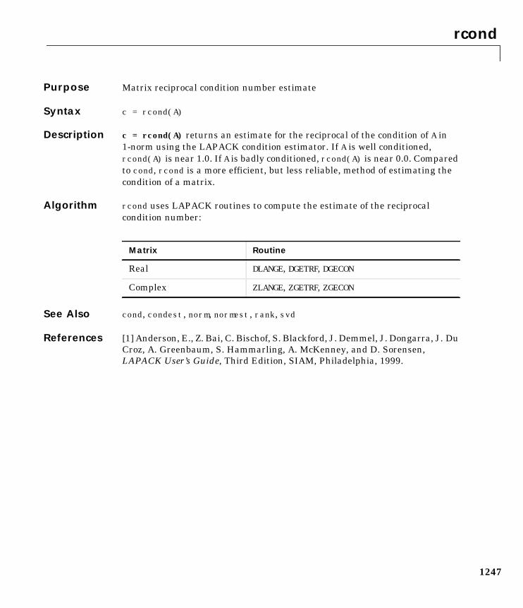
rcond
1247
1rcondPurpose Matrix reciprocal condition number estimate
Syntax c = rcond(A)
Description c = rcond(A) returns an estimate for the reciprocal of the condition of A in1-norm using the LAPACK condition estimator. If A is well conditioned,rcond(A) is near 1.0. If A is badly conditioned, rcond(A) is near 0.0. Comparedto cond, rcond is a more efficient, but less reliable, method of estimating thecondition of a matrix.
Algorithm rcond uses LAPACK routines to compute the estimate of the reciprocalcondition number:
See Also cond, condest, norm, normest, rank, svd
References [1] Anderson, E., Z. Bai, C. Bischof, S. Blackford, J. Demmel, J. Dongarra, J. DuCroz, A. Greenbaum, S. Hammarling, A. McKenney, and D. Sorensen,LAPACK User’s Guide, Third Edition, SIAM, Philadelphia, 1999.
Matrix Routine
Real DLANGE, DGETRF, DGECON
Complex ZLANGE, ZGETRF, ZGECON
readasync
1248
1readasyncPurpose Read data asynchronously from the device
Syntax readasync(obj)readasync(obj,size)
Arguments
Description readasync(obj) initiates an asynchronous read operation.
readasync(obj,size) asynchronously reads, at most, the number of bytesgiven by size. If size is greater than the difference between theInputBufferSize property value and the BytesAvailable property value, anerror is returned.
Remarks Before you can read data, you must connect obj to the device with the fopenfunction. A connected serial port object has a Status property value of open. Anerror is returned if you attempt to perform a read operation while obj is notconnected to the device.
You should use readasync only when you configure the ReadAsyncModeproperty to manual. readasync is ignored if used when ReadAsyncMode iscontinuous.
The TransferStatus property indicates if an asynchronous read or writeoperation is in progress. You can write data while an asynchronous read is inprogress since serial ports have separate read and write pins. You can stopasynchronous read and write operations with the stopasync function.
You can monitor the amount of data stored in the input buffer with theBytesAvailable property. Additionally, you can use theBytesAvailableAction property to execute an M-file action function when theterminator or the specified amount of data is read.
Rules for Completing an Asynchronous Read OperationAn asynchronous read operation with readasync completes when one of theseconditions is met:
• The terminator specified by the Terminator property is read.
obj A serial port object.
size The number of bytes to read from the device.
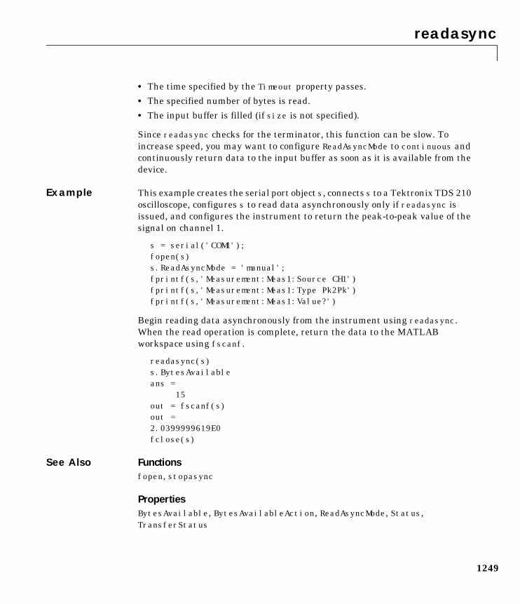
readasync
1249
• The time specified by the Timeout property passes.
• The specified number of bytes is read.
• The input buffer is filled (if size is not specified).
Since readasync checks for the terminator, this function can be slow. Toincrease speed, you may want to configure ReadAsyncMode to continuous andcontinuously return data to the input buffer as soon as it is available from thedevice.
Example This example creates the serial port object s, connects s to a Tektronix TDS 210oscilloscope, configures s to read data asynchronously only if readasync isissued, and configures the instrument to return the peak-to-peak value of thesignal on channel 1.
s = serial('COM1');fopen(s)s.ReadAsyncMode = 'manual';fprintf(s,'Measurement:Meas1:Source CH1')fprintf(s,'Measurement:Meas1:Type Pk2Pk')fprintf(s,'Measurement:Meas1:Value?')
Begin reading data asynchronously from the instrument using readasync.When the read operation is complete, return the data to the MATLABworkspace using fscanf.
readasync(s)s.BytesAvailableans = 15out = fscanf(s)out =2.0399999619E0fclose(s)
See Also Functionsfopen, stopasync
PropertiesBytesAvailable, BytesAvailableAction, ReadAsyncMode, Status,TransferStatus
real
1250
1realPurpose Real part of complex number
Syntax X = real(Z)
Description X = real(Z) returns the real part of the elements of the complex array Z.
Examples real(2+3*i) is 2.
See Also abs, angle, conj, i, j, imag
realmax
1251
1realmaxPurpose Largest positive floating-point number
Syntax n = realmax
Description n = realmax returns the largest floating-point number representable on aparticular computer. Anything larger overflows.
Examples realmax is one bit less than 21024 or about 1.7977e+308.
Algorithm The realmax function is equivalent to pow2(2-eps,maxexp), where maxexp isthe largest possible floating-point exponent.
Execute type realmax to see maxexp for various computers.
See Also eps, realmin
realmin
1252
1realminPurpose Smallest positive floating-point number
Syntax n = realmin
Description n = realmin returns the smallest positive normalized floating-point numberon a particular computer. Anything smaller underflows or is an IEEE“denormal.”
Examples On machines with IEEE floating-point format, realmin is 2^(-1022) or about2.2251e-308.
Algorithm The realmin function is equivalent to pow2(1,minexp) where minexp is thesmallest possible floating-point exponent.
Execute type realmin to see minexp for various computers.
See Also eps, realmax
record
1253
1recordPurpose Record data and event information to a file
Syntax record(obj)record(obj,'switch')
Arguments
Description record(obj) toggles the recording state for obj.
record(obj,'switch') initiates or terminates recording for obj. switch canbe on or off. If switch is on, recording is initiated. If switch is off, recordingis terminated.
Remarks Before you can record information to disk, obj must be connected to the devicewith the fopen function. A connected serial port object has a Status propertyvalue of open. An error is returned if you attempt to record information whileobj is not connected to the device. Each serial port object must recordinformation to a separate file. Recording is automatically terminated when objis disconnected from the device with fclose.
The RecordName and RecordMode properties are read-only while obj isrecording, and must be configured before using record.
For a detailed description of the record file format and the propertiesassociated with recording data and event information to a file, refer to“Recording Information to Disk” on page 8-62.
Example This example creates the serial port object s, connects s to the device,configures s to record information to a file, writes and reads text data, and thendisconnects s from the device.
s = serial('COM1');fopen(s)s.RecordDetail = 'verbose';s.RecordName = 'MySerialFile.txt';record(s,'on')fprintf(s,'*IDN?')out = fscanf(s);
obj A serial port object.
'switch' Switch recording capabilities on or off.
record
1254
record(s,'off')fclose(s)
See Also Functionsfclose, fopen
PropertiesRecordDetail, RecordMode, RecordName, RecordStatus, Status
rectangle
1255
1rectanglePurpose C reate a 2-D rectangle object
Syntax rectanglerectangle('Position',[x,y,w,h])rectangle(...,'Curvature',[x,y])h = rectangle(...)
Description rectangle draws a rectangle with Position [0,0,1,1] and Curvature [0,0](i.e., no curvature).
rectangle('Position',[x,y,w,h]) draws the rectangle from the point x,yand having a width of w and a height of h. Specify values in axes data units.
Note that, to display a rectangle in the specified proportions, you need to setthe axes data aspect ratio so that one unit is of equal length along both the xand y axes. You can do this with the command axis equal ordaspect([1,1,1]).
rectangle(...,'Curvature',[x,y]) specifies the curvature of the rectanglesides, enabling it to vary from a rectangle to an ellipse. The horizontalcurvature x is the fraction of width of the rectangle that is curved along the topand bottom edges. The vertical curvature y is the fraction of the height of therectangle that is curved along the left and right edges.
The values of x and y can range from 0 (no curvature) to 1 (maximumcurvature). A value of [0,0] creates a rectangle with square sides. A value of[1,1] creates an ellipse. If you specify only one value for Curvature, then thesame length (in axes data units) is curved along both horizontal and verticalsides. The amount of curvature is determined by the shorter dimension.
h = rectangle(...) returns the handle of the rectangle object created.
Remarks Rectangle objects are 2-D and can be drawn in an axes only if the view is [090] (i.e., view(2)). Rectangles are children of axes and are defined incoordinates of the axes data.
Examples This example sets the data aspect ratio to [1,1,1] so that the rectangledisplays in the specified proportions (daspect). Note that the horizontal and
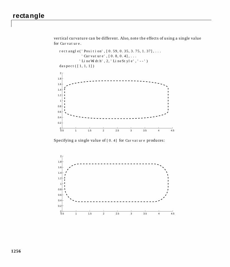
rectangle
1256
vertical curvature can be different. Also, note the effects of using a single valuefor Curvature.
rectangle('Position',[0.59,0.35,3.75,1.37],...'Curvature',[0.8,0.4],...
'LineWidth',2,'LineStyle','--')daspect([1,1,1])
Specifying a single value of [0.4] for Curvature produces:
0.5 1 1.5 2 2.5 3 3.5 4 4.50
0.2
0.4
0.6
0.8
1
1.2
1.4
1.6
1.8
2
0.5 1 1.5 2 2.5 3 3.5 4 4.50
0.2
0.4
0.6
0.8
1
1.2
1.4
1.6
1.8
2
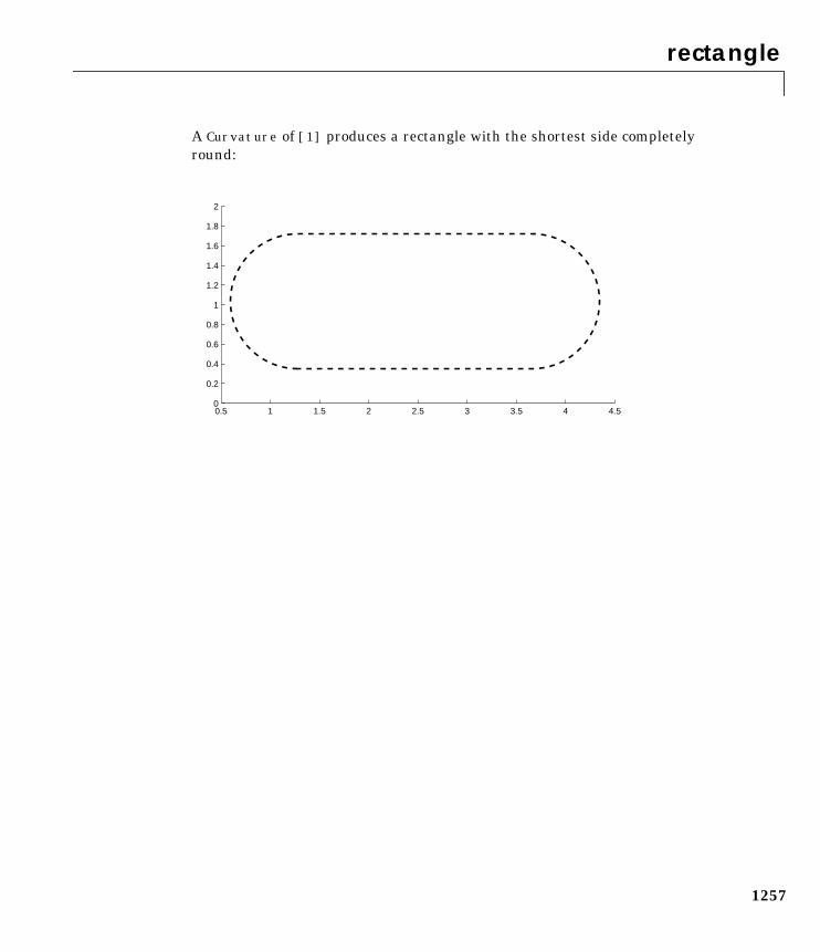
rectangle
1257
A Curvature of [1] produces a rectangle with the shortest side completelyround:
0.5 1 1.5 2 2.5 3 3.5 4 4.50
0.2
0.4
0.6
0.8
1
1.2
1.4
1.6
1.8
2
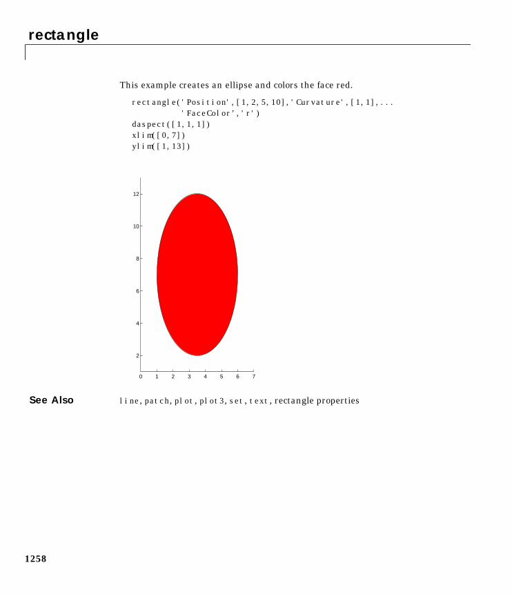
rectangle
1258
This example creates an ellipse and colors the face red.
rectangle('Position',[1,2,5,10],'Curvature',[1,1],...'FaceColor’,'r')
daspect([1,1,1])xlim([0,7])ylim([1,13])
See Also line, patch, plot, plot3, set, text, rectangle properties
0 1 2 3 4 5 6 7
2
4
6
8
10
12
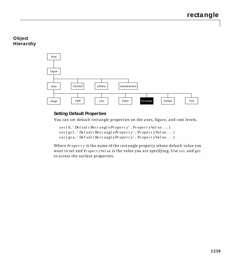
rectangle
1259
ObjectHierarchy
Setting Default PropertiesYou can set default rectangle properties on the axes, figure, and root levels.
set(0,'DefaultRectangleProperty',PropertyValue...)set(gcf,'DefaultRectangleProperty',PropertyValue...)set(gca,'DefaultRectangleProperty',PropertyValue...)
Where Property is the name of the rectangle property whose default value youwant to set and PropertyValue is the value you are specifying. Use set and getto access the surface properties.
Uimenu
Line
Axes Uicontrol
Image
Figure
Uicontextmenu
Light SurfacePatch Text
Root
Rectangle
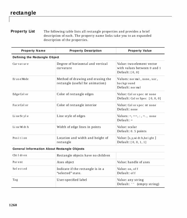
rectangle
1260
Property List The following table lists all rectangle properties and provides a briefdescription of each. The property name links take you to an expandeddescription of the properties.
Property Name Property Description Property Value
Defining the Rectangle Object
Curvature Degree of horizontal and verticalcurvature
Value: two-element vectorwith values between 0 and 1Default: [0,0]
EraseMode Method of drawing and erasing therectangle (useful for animation)
Values: normal, none, xor,backgroundDefault: normal
EdgeColor Color of rectangle edges Value: Colorspec or noneDefault: ColorSpec [0,0,0]
FaceColor Color of rectangle interior Value: Colorspec or noneDefault: none
LineStyle Line style of edges Values: −, −− , :, −., noneDefault: −
LineWidth Width of edge lines in points Value: scalarDefault: 0.5 points
Position Location and width and height ofrectangle
Value: [x,y,width,height]Default: [0,0,1,1]
General Information About Rectangle Objects
Children Rectangle objects have no children
Parent Axes object Value: handle of axes
Selected Indicate if the rectangle is in a“selected” state.
Value: on, offDefault: off
Tag User-specified label Value: any stringDefault: '' (empty string)
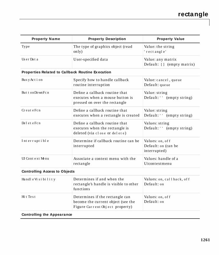
rectangle
1261
Type The type of graphics object (readonly)
Value: the string'rectangle'
UserData User-specified data Value: any matrixDefault: [] (empty matrix)
Properties Related to Callback Routine Execution
BusyAction Specify how to handle callbackroutine interruption
Value: cancel, queueDefault: queue
ButtonDownFcn Define a callback routine thatexecutes when a mouse button ispressed on over the rectangle
Value: stringDefault: '' (empty string)
CreateFcn Define a callback routine thatexecutes when a rectangle is created
Value: stringDefault: '' (empty string)
DeleteFcn Define a callback routine thatexecutes when the rectangle isdeleted (via close or delete)
Values: stringDefault: '' (empty string)
Interruptible Determine if callback routine can beinterrupted
Values: on, offDefault: on (can beinterrupted)
UIContextMenu Associate a context menu with therectangle
Values: handle of aUicontextmenu
Controlling Access to Objects
HandleVisibility Determines if and when therectangle’s handle is visible to otherfunctions
Values: on, callback, offDefault: on
HitTest Determines if the rectangle canbecome the current object (see theFigure CurrentObject property)
Values: on, offDefault: on
Controlling the Appearance
Property Name Property Description Property Value
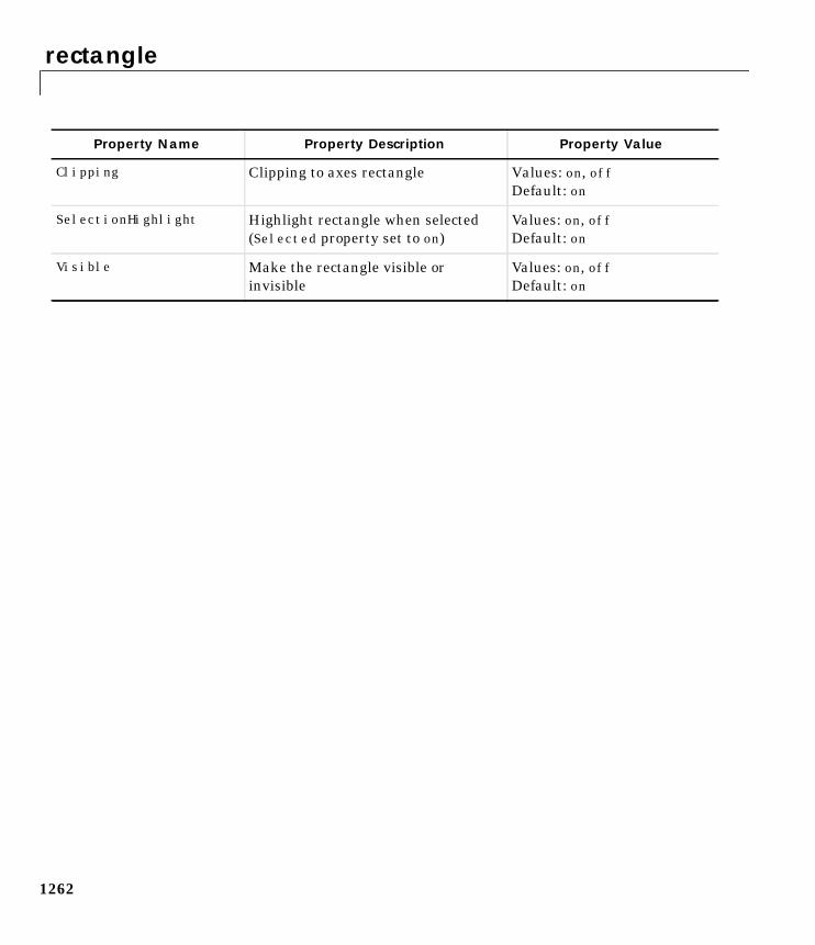
rectangle
1262
Clipping Clipping to axes rectangle Values: on, offDefault: on
SelectionHighlight Highlight rectangle when selected(Selected property set to on)
Values: on, offDefault: on
Visible Make the rectangle visible orinvisible
Values: on, offDefault: on
Property Name Property Description Property Value
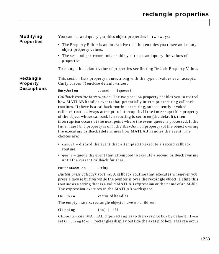
rectangle properties
1263
1rectangle propertiesModifyingProperties
You can set and query graphics object properties in two ways:
• The Property Editor is an interactive tool that enables you to see and changeobject property values.
• The set and get commands enable you to set and query the values ofproperties
To change the default value of properties see Setting Default Property Values.
RectanglePropertyDescriptions
This section lists property names along with the type of values each accepts.Curly braces enclose default values.
BusyAction cancel | queue
Callback routine interruption. The BusyAction property enables you to controlhow MATLAB handles events that potentially interrupt executing callbackroutines. If there is a callback routine executing, subsequently invokedcallback routes always attempt to interrupt it. If the Interruptible propertyof the object whose callback is executing is set to on (the default), theninterruption occurs at the next point where the event queue is processed. If theInterruptible property is off, the BusyAction property (of the object owningthe executing callback) determines how MATLAB handles the event. Thechoices are:
• cancel – discard the event that attempted to execute a second callbackroutine.
• queue – queue the event that attempted to execute a second callback routineuntil the current callback finishes.
ButtonDownFcn string
Button press callback routine. A callback routine that executes whenever youpress a mouse button while the pointer is over the rectangle object. Define thisroutine as a string that is a valid MATLAB expression or the name of an M-file.The expression executes in the MATLAB workspace.
Children vector of handles
The empty matrix; rectangle objects have no children.
Clipping on | off
Clipping mode. MATLAB clips rectangles to the axes plot box by default. If youset Clipping to off, rectangles display outside the axes plot box. This can occur
rectangle properties
1264
if you create a rectangle, set hold to on, freeze axis scaling (axis manual), andthen create a larger rectangle.
CreateFcn string
Callback routine executed during object creation. This property defines acallback routine that executes when MATLAB creates a rectangle object. Youmust define this property as a default value for rectangles. For example, thestatement,
set(0,'DefaultRectangleCreateFcn',...
'set(gca,''DataAspectRatio'',[1,1,1])')
defines a default value on the root level that sets the axes DataAspectRatiowhenever you create a rectangle object. MATLAB executes this routine aftersetting all rectangle properties. Setting this property on an existing rectangleobject has no effect.
The handle of the object whose CreateFcn is being executed is accessible onlythrough the root CallbackObject property, which you can query using gcbo.
Curvature one- or two-element vector [x,y]
Amount of horizontal and vertical curvature. This property specifies thecurvature of the property sides, which enables the shape of the rectangle tovary from rectangular to ellipsoidal. The horizontal curvature x is the fractionof width of the rectangle that is curved along the top and bottom edges. Thevertical curvature y is the fraction of the height of the rectangle that is curvedalong the left and right edges.
The values of x and y can range from 0 (no curvature) to 1 (maximumcurvature). A value of [0,0] creates a rectangle with square sides. A value of[1,1] creates an ellipse. If you specify only one value for Curvature, then thesame length (in axes data units) is curved along both horizontal and verticalsides. The amount of curvature is determined by the shorter dimension.
DeleteFcn string
Delete rectangle callback routine. A callback routine that executes when youdelete the rectangle object (e.g., when you issue a delete command or clear theaxes or figure). MATLAB executes the routine before deleting the object’sproperties so these values are available to the callback routine.
rectangle properties
1265
The handle of the object whose DeleteFcn is being executed is accessible onlythrough the root CallbackObject property, which you can query using gcbo.
EdgeColor Colorspec | none
Color of the rectangle edges. This property specifies the color of the rectangleedges as a color or specifies that no edges be drawn.
EraseMode normal | none | xor | background
Erase mode. This property controls the technique MATLAB uses to draw anderase rectangle objects. Alternative erase modes are useful for creatinganimated sequences, where control of the way individual objects redraw isnecessary to improve performance and obtain the desired effect.
• normal (the default) – Redraw the affected region of the display, performingthe three-dimensional analysis necessary to ensure that all objects arerendered correctly. This mode produces the most accurate picture, but is theslowest. The other modes are faster, but do not perform a complete redrawand are therefore less accurate.
• none – Do not erase the rectangle when it is moved or destroyed. While theobject is still visible on the screen after erasing with EraseMode none, youcannot print it because MATLAB stores no information about its formerlocation.
• xor – Draw and erase the rectangle by performing an exclusive OR (XOR)with the color of the screen beneath it. This mode does not damage the colorof the objects beneath the rectangle. However, the rectangle’s color dependson the color of whatever is beneath it on the display.
• background – Erase the rectangle by drawing it in the Axes’ backgroundColor, or the Figure background Color if the Axes Color is set to none. Thisdamages objects that are behind the erased rectangle, but rectangles arealways properly colored.
Printing with Non-normal Erase Modes.
MATLAB always prints Figures as if the EraseMode of all objects is normal.This means graphics objects created with EraseMode set to none, xor, orbackground can look different on screen than on paper. On screen, MATLABmay mathematically combine layers of colors (e.g., XORing a pixel color withthat of the pixel behind it) and ignore three-dimensional sorting to obtain
rectangle properties
1266
greater rendering speed. However, these techniques are not applied to theprinted output.
You can use the MATLAB getframe command or other screen captureapplication to create an image of a Figure containing non-normal mode objects.
FaceColor ColorSpec | none
Color of rectangle face. This property specifies the color of the rectangle face,which is not colored by default.
HandleVisibility on | callback | off
Control access to object’s handle by command-line users and GUIs. Thisproperty determines when an object’s handle is visible in its parent’s list ofchildren. HandleVisibility is useful for preventing command-line users fromaccidentally drawing into or deleting a figure that contains only user interfacedevices (such as a dialog box).
Handles are always visible when HandleVisibility is on.
Setting HandleVisibility to callback causes handles to be visible fromwithin callback routines or functions invoked by callback routines, but not fromwithin functions invoked from the command line. This provides a means toprotect GUIs from command-line users, while allowing callback routines tohave complete access to object handles.
Setting HandleVisibility to off makes handles invisible at all times. Thismay be necessary when a callback routine invokes a function that mightpotentially damage the GUI (such as evaling a user-typed string), and sotemporarily hides its own handles during the execution of that function.
When a handle is not visible in its parent’s list of children, it cannot be returnedby functions that obtain handles by searching the object hierarchy or queryinghandle properties. This includes get, findobj, gca, gcf, gco, newplot, cla, clf,and close.
When a handle’s visibility is restricted using callback or off, the object’shandle does not appear in its parent’s Children property, figures do not appearin the root’s CurrentFigure property, objects do not appear in the root’sCallbackObject property or in the figure’s CurrentObject property, and Axesdo not appear in their parent’s CurrentAxes property.
rectangle properties
1267
You can set the Root ShowHiddenHandles property to on to make all handlesvisible, regardless of their HandleVisibility settings (this does not affect thevalues of the HandleVisibility properties).
Handles that are hidden are still valid. If you know an object’s handle, you canset and get its properties, and pass it to any function that operates on handles.
HitTest on | off
Selectable by mouse click. HitTest determines if the rectangle can become thecurrent object (as returned by the gco command and the figure CurrentObjectproperty) as a result of a mouse click on the rectangle. If HitTest is off,clicking on the rectangle selects the object below it (which may be the axescontaining it).
Interruptible on | off
Callback routine interruption mode. The Interruptible property controlswhether a rectangle callback routine can be interrupted by subsequentlyinvoked callback routines. Only callback routines defined for theButtonDownFcn are affected by the Interruptible property. MATLAB checksfor events that can interrupt a callback routine only when it encounters adrawnow, figure, getframe, or pause command in the routine.
LineStyle − | −− | : | −. | none
Line style. This property specifies the line style of the edges. The available linestyles are:
Symbol Line Style
− solid line (default)
−− dashed line
: dotted line
−. dash-dot line
none no line
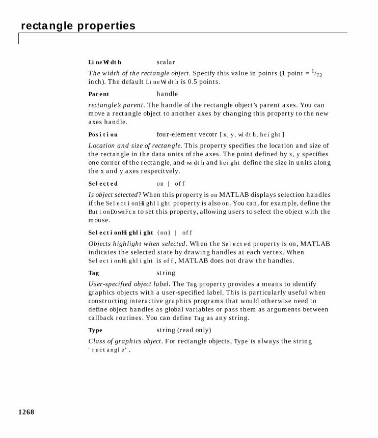
rectangle properties
1268
LineWidth scalar
The width of the rectangle object. Specify this value in points (1 point = 1/72inch). The default LineWidth is 0.5 points.
Parent handle
rectangle’s parent. The handle of the rectangle object’s parent axes. You canmove a rectangle object to another axes by changing this property to the newaxes handle.
Position four-element vecotr [x,y,width,height]
Location and size of rectangle. This property specifies the location and size ofthe rectangle in the data units of the axes. The point defined by x, y specifiesone corner of the rectangle, and width and height define the size in units alongthe x and y axes respecitvely.
Selected on | off
Is object selected? When this property is onMATLAB displays selection handlesif the SelectionHighlight property is also on. You can, for example, define theButtonDownFcn to set this property, allowing users to select the object with themouse.
SelectionHighlight on | off
Objects highlight when selected. When the Selected property is on, MATLABindicates the selected state by drawing handles at each vertex. WhenSelectionHighlight is off, MATLAB does not draw the handles.
Tag string
User-specified object label. The Tag property provides a means to identifygraphics objects with a user-specified label. This is particularly useful whenconstructing interactive graphics programs that would otherwise need todefine object handles as global variables or pass them as arguments betweencallback routines. You can define Tag as any string.
Type string (read only)
Class of graphics object. For rectangle objects, Type is always the string'rectangle'.
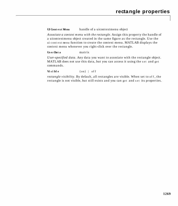
rectangle properties
1269
UIContextMenu handle of a uicontextmenu object
Associate a context menu with the rectangle. Assign this property the handle ofa uicontextmenu object created in the same figure as the rectangle. Use theuicontextmenu function to create the context menu. MATLAB displays thecontext menu whenever you right-click over the rectangle.
UserData matrix
User-specified data. Any data you want to associate with the rectangle object.MATLAB does not use this data, but you can access it using the set and getcommands.
Visible on | off
rectangle visibility. By default, all rectangles are visible. When set to off, therectangle is not visible, but still exists and you can get and set its properties.
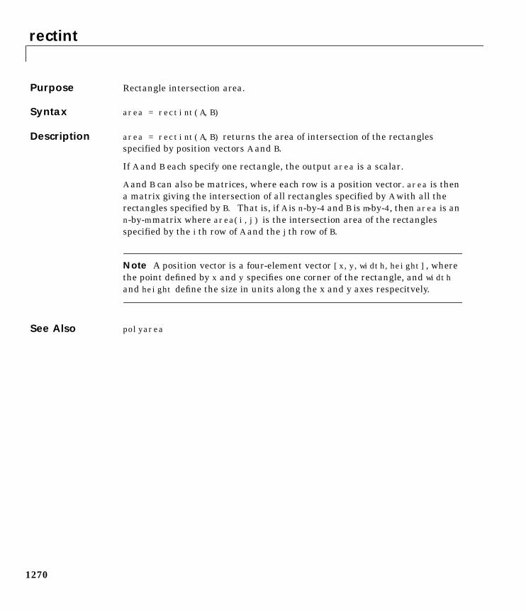
rectint
1270
1rectintPurpose Rectangle intersection area.
Syntax area = rectint(A,B)
Description area = rectint(A,B) returns the area of intersection of the rectanglesspecified by position vectors A and B.
If A and B each specify one rectangle, the output area is a scalar.
A and B can also be matrices, where each row is a position vector. area is thena matrix giving the intersection of all rectangles specified by A with all therectangles specified by B. That is, if A is n-by-4 and B is m-by-4, then area is ann-by-m matrix where area(i,j) is the intersection area of the rectanglesspecified by the ith row of A and the jth row of B.
Note A position vector is a four-element vector [x,y,width,height], wherethe point defined by x and y specifies one corner of the rectangle, and widthand height define the size in units along the x and y axes respecitvely.
See Also polyarea
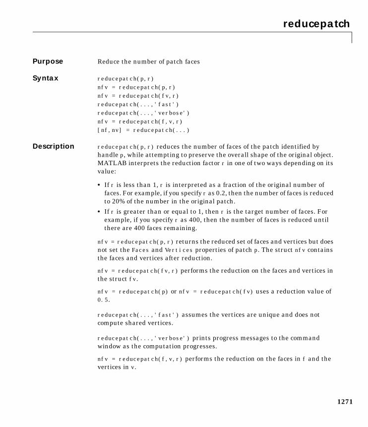
reducepatch
1271
1reducepatchPurpose Reduce the number of patch faces
Syntax reducepatch(p,r)nfv = reducepatch(p,r)nfv = reducepatch(fv,r)reducepatch(...,'fast')reducepatch(...,'verbose')nfv = reducepatch(f,v,r)[nf,nv] = reducepatch(...)
Description reducepatch(p,r) reduces the number of faces of the patch identified byhandle p, while attempting to preserve the overall shape of the original object.MATLAB interprets the reduction factor r in one of two ways depending on itsvalue:
• If r is less than 1, r is interpreted as a fraction of the original number offaces. For example, if you specify r as 0.2, then the number of faces is reducedto 20% of the number in the original patch.
• If r is greater than or equal to 1, then r is the target number of faces. Forexample, if you specify r as 400, then the number of faces is reduced untilthere are 400 faces remaining.
nfv = reducepatch(p,r) returns the reduced set of faces and vertices but doesnot set the Faces and Vertices properties of patch p. The struct nfv containsthe faces and vertices after reduction.
nfv = reducepatch(fv,r) performs the reduction on the faces and vertices inthe struct fv.
nfv = reducepatch(p) or nfv = reducepatch(fv) uses a reduction value of0.5.
reducepatch(...,'fast') assumes the vertices are unique and does notcompute shared vertices.
reducepatch(...,'verbose') prints progress messages to the commandwindow as the computation progresses.
nfv = reducepatch(f,v,r) performs the reduction on the faces in f and thevertices in v.
reducepatch
1272
[nf,nv] = reducepatch(...) returns the faces and vertices in the arrays nfand nv.
Remarks If the patch contains nonshared vertices, MATLAB computes shared verticesbefore reducing the number of faces. If the faces of the patch are not triangles,MATLAB triangulates the faces before reduction. The faces returned arealways defined as triangles.
The number of output triangles may not be exactly the number specified withthe reduction factor argument (r), particularly if the faces of the original patchare not triangles.
Examples This example illustrates the effect of reducing the number of faces to only 15%of the original value.
[x,y,z,v] = flow;p = patch(isosurface(x,y,z,v,-3));set(p,'facecolor','w','EdgeColor','b');daspect([1,1,1])view(3)figure;h = axes;p2 = copyobj(p,h);reducepatch(p2,0.15)daspect([1,1,1])view(3)
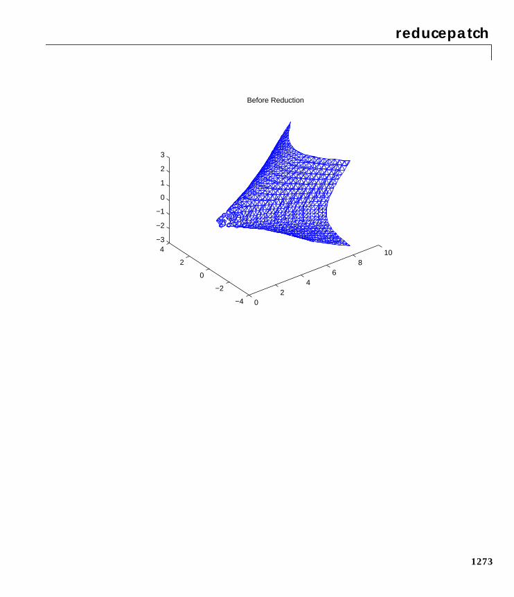
reducepatch
1273
02
46
810
−4
−2
0
2
4−3
−2
−1
0
1
2
3
Before Reduction
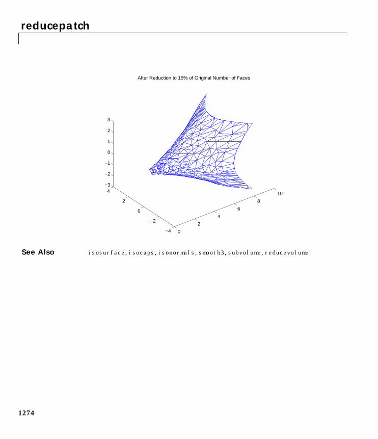
reducepatch
1274
See Also isosurface, isocaps, isonormals, smooth3, subvolume, reducevolume
0
2
4
6
8
10
−4
−2
0
2
4−3
−2
−1
0
1
2
3
After Reduction to 15% of Original Number of Faces
reducevolume
1275
1reducevolumePurpose Reduce the number of elements in a volume data set
Syntax [nx,ny,nz,nv] = reducevolume(X,Y,Z,V,[Rx,Ry,Rz])[nx,ny,nz,nv] = reducevolume(V,[Rx,Ry,Rz])nv = reducevolume(...)
Description [nx,ny,nz,nv] = reducevolume(X,Y,Z,V,[Rx,Ry,Rz]) reduces the numberof elements in the volume by retaining every Rxth element in the x direction,every Ryth element in the y direction, and every Rzth element in the z direction.If a scalar R is used to indicate the amount or reduction instead of a 3-elementvector, MATLAB assumes the reduction to be [R R R].
The arrays X, Y, and Z define the coordinates for the volume V. The reducedvolume is returned in nv and the coordinates of the reduced volume arereturned in nx, ny, and nz.
[nx,ny,nz,nv] = reducevolume(V,[Rx,Ry,Rz]) assumes the arrays X, Y, andZ are defined as [X,Y,Z] = meshgrid(1:n,1:m,1:p) where [m,n,p] =size(V).
nv = reducevolume(...) returns only the reduced volume.
Examples This example uses a data set that is a collection of MRI slices of a human skull.This data is processed in a variety of ways:
• The 4-D array is squeezed (squeeze) into three dimensions and then reduced(reducevolume) so that what remains is every 4th element in the x and ydirections and every element in the z direction.
• The reduced data is smoothed (smooth3).
• The outline of the skull is an isosurface generated as a patch (p1) whosevertex normals are recalculated to improve the appearance when lighting isapplied (patch, isosurface, isonormals).
• A second patch (p2) with an interpolated face color draws the end caps(FaceColor, isocaps).
• The view of the object is set (view, axis, daspect).
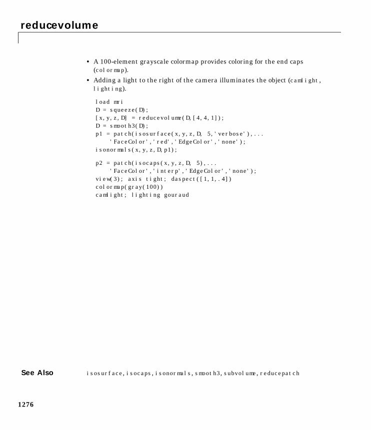
reducevolume
1276
• A 100-element grayscale colormap provides coloring for the end caps(colormap).
• Adding a light to the right of the camera illuminates the object (camlight,lighting).
load mriD = squeeze(D);[x,y,z,D] = reducevolume(D,[4,4,1]);D = smooth3(D);p1 = patch(isosurface(x,y,z,D, 5,'verbose'),... 'FaceColor','red','EdgeColor','none');isonormals(x,y,z,D,p1);
p2 = patch(isocaps(x,y,z,D, 5),...'FaceColor','interp','EdgeColor','none');
view(3); axis tight; daspect([1,1,.4])colormap(gray(100))camlight; lighting gouraud
See Also isosurface, isocaps, isonormals, smooth3, subvolume, reducepatch
refresh
1277
1refreshPurpose Redraw current figure
Syntax refreshrefresh(h)
Description refresh erases and redraws the current figure.
refresh(h) redraws the figure identified by h.
rehash
1278
1rehashPurpose Refresh function and file system caches
Syntax rehashrehash pathrehash toolboxrehash pathresetrehash toolboxresetrehash toolboxcache
Description rehash performs the same refresh that is done whenever MATLAB completesa command and returns to its prompt. The rehash function rereads changeddirectories, refreshes the list of known classes, and, if there are any functionswhose source files have changed since they were loaded into memory, rehashclears those loaded functions.
rehash path is the same as rehash, except that it unconditionally rereads allnontoolbox directories. This is exactly the same as the behavior of path(path).
rehash toolbox is the same as rehash path, except that it unconditionallyrereads all directories, including all toolbox directories.
rehash pathreset is the same as rehash path, except that it also forces anyshadowed functions to be replaced by any shadowing functions.
rehash toolboxreset is the same as rehash toolbox, except that it also forcesany shadowed functions to be replaced by any shadowing functions. This is thesame as exiting and restarting MATLAB.
rehash toolboxcache generates a new toolbox cache. To use this command,you must first enable toolbox caching on your system. You also need read andwrite access to the directory that holds the toolbox cache file.
See Also path, addpath, rmpath
Relational Operators < > <= >= == ~=
1279
1Relational Operators < > <= >= == ~=Purpose Relational operations
Syntax A < BA > BA <= BA >= BA == BA ~= B
Description The relational operators are <, ≤, >, ≥, ==, and ~=. Relational operators performelement-by-element comparisons between two arrays. They return an array ofthe same size, with elements set to logical true (1) where the relation is true,and elements set to logical false (0) where it is not.
The operators <, ≤, >, and ≥ use only the real part of their operands for thecomparison. The operators == and ~= test real and imaginary parts.
To test if two strings are equivalent, use strcmp, which allows vectors ofdissimilar length to be compared.
Examples If one of the operands is a scalar and the other a matrix, the scalar expands tothe size of the matrix. For example, the two pairs of statements:
X = 5; X >= [1 2 3; 4 5 6; 7 8 10]X = 5∗ones(3,3); X >= [1 2 3; 4 5 6; 7 8 10]
produce the same result:
ans =
1 1 11 1 00 0 0
Relational Operators < > <= >= == ~=
1280
See Also all, any, find, strcmp
The logical operators &, |, ~
rem
1281
1remPurpose Remainder after division
Syntax R = rem(X,Y)
Description R = rem(X,Y) returns X - fix(X./Y).∗Y, where fix(X./Y) is the integer partof the quotient, X./Y.
Remarks So long as operands X and Y are of the same sign, the statement rem(X,Y)returns the same result as does mod(X,Y). However, for positive X and Y,
rem(-x,y) = mod(-x,y)-y
The rem function returns a result that is between 0 and sign(X)*abs(Y). If Yis zero, rem returns NaN.
Limitations Arguments X and Y should be integers. Due to the inexact representation offloating-point numbers on a computer, real (or complex) inputs may lead tounexpected results.
See Also mod
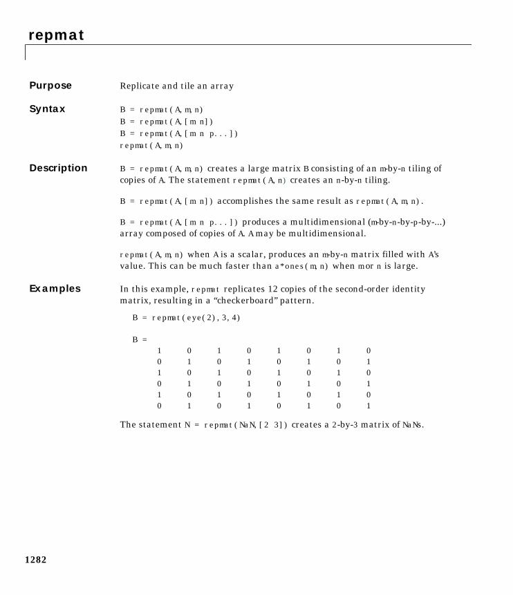
repmat
1282
1repmatPurpose Replicate and tile an array
Syntax B = repmat(A,m,n)B = repmat(A,[m n])B = repmat(A,[m n p...])repmat(A,m,n)
Description B = repmat(A,m,n) creates a large matrix B consisting of an m-by-n tiling ofcopies of A. The statement repmat(A,n) creates an n-by-n tiling.
B = repmat(A,[m n]) accomplishes the same result as repmat(A,m,n).
B = repmat(A,[m n p...]) produces a multidimensional (m-by-n-by-p-by-...)array composed of copies of A. A may be multidimensional.
repmat(A,m,n) when A is a scalar, produces an m-by-n matrix filled with A’svalue. This can be much faster than a*ones(m,n) when m or n is large.
Examples In this example, repmat replicates 12 copies of the second-order identitymatrix, resulting in a “checkerboard” pattern.
B = repmat(eye(2),3,4)
B = 1 0 1 0 1 0 1 0 0 1 0 1 0 1 0 1 1 0 1 0 1 0 1 0 0 1 0 1 0 1 0 1 1 0 1 0 1 0 1 0 0 1 0 1 0 1 0 1
The statement N = repmat(NaN,[2 3]) creates a 2-by-3 matrix of NaNs.
reset
1283
1resetPurpose Reset graphics object properties to their defaults
Syntax reset(h)
Description reset(h) resets all properties having factory defaults on the object identifiedby h. To see the list of factory defaults, use the statement,
get(0,'factory')
If h is a figure, MATLAB does not reset Position, Units, PaperPosition, andPaperUnits. If h is an axes, MATLAB does not reset Position and Units.
Examples reset(gca) resets the properties of the current axes.
reset(gcf) resets the properties of the current figure.
See Also cla, clf, gca, gcf, hold
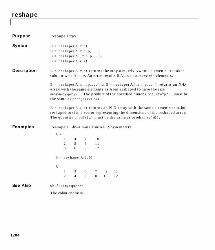
reshape
1284
1reshapePurpose Reshape array
Syntax B = reshape(A,m,n)B = reshape(A,m,n,p,...)B = reshape(A,[m n p...])B = reshape(A,siz)
Description B = reshape(A,m,n) returns the m-by-n matrix B whose elements are takencolumn-wise from A. An error results if A does not have m∗n elements.
B = reshape(A,m,n,p,...) or B = reshape(A,[m n p...]) returns an N-Darray with the same elements as A but reshaped to have the sizem-by-n-by-p-by-... . The product of the specified dimensions, m*n*p*..., must bethe same as prod(size(A)).
B = reshape(A,siz) returns an N-D array with the same elements as A, butreshaped to siz, a vector representing the dimensions of the reshaped array.The quantity prod(siz) must be the same as prod(size(A)).
Examples Reshape a 3-by-4 matrix into a 2-by-6 matrix:
A = 1 4 7 10 2 5 8 11 3 6 9 12
B = reshape(A,2,6)
B = 1 3 5 7 9 11 2 4 6 8 10 12
See Also shiftdim, squeeze
The colon operator :
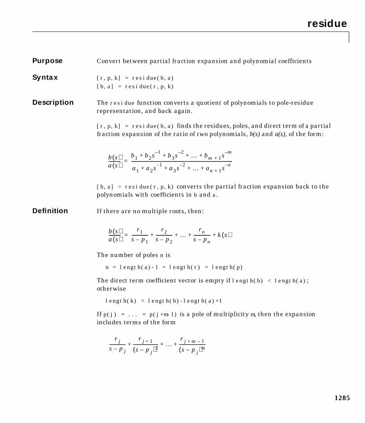
residue
1285
1residuePurpose Convert between partial fraction expansion and polynomial coefficients
Syntax [r,p,k] = residue(b,a)[b,a] = residue(r,p,k)
Description The residue function converts a quotient of polynomials to pole-residuerepresentation, and back again.
[r,p,k] = residue(b,a) finds the residues, poles, and direct term of a partialfraction expansion of the ratio of two polynomials, b(s) and a(s), of the form:
[b,a] = residue(r,p,k) converts the partial fraction expansion back to thepolynomials with coefficients in b and a.
Definition If there are no multiple roots, then:
The number of poles n is
n = length(a)-1 = length(r) = length(p)
The direct term coefficient vector is empty if length(b) < length(a);otherwise
length(k) = length(b)-length(a)+1
If p(j) = ... = p(j+m-1) is a pole of multiplicity m, then the expansionincludes terms of the form
b s( )a s( )-----------
b1 b2s 1– b3s 2– … bm 1+ s m–+ + + +
a1 a2s 1– a3s 2– … an 1+ s n–+ + + +
---------------------------------------------------------------------------------------------=
b s( )a s( )-----------
r1s p1–---------------
r2s p2–--------------- …
rns pn–--------------- k s( )+ + + +=
r js p j–---------------
r j 1+
s p j–( )2----------------------- …
r j m 1–+
s p j–( )m------------------------+ + +
residue
1286
Arguments
Algorithm The residue function is an M-file. It first obtains the poles with roots. Next, ifthe fraction is nonproper, the direct term k is found using deconv, whichperforms polynomial long division. Finally, the residues are determined byevaluating the polynomial with individual roots removed. For repeated roots,the M-file resi2 computes the residues at the repeated root locations.
Limitations Numerically, the partial fraction expansion of a ratio of polynomials representsan ill-posed problem. If the denominator polynomial, a(s), is near a polynomialwith multiple roots, then small changes in the data, including roundoff errors,can make arbitrarily large changes in the resulting poles and residues.Problem formulations making use of state-space or zero-pole representationsare preferable.
See Also deconv, poly, roots
References [1] Oppenheim, A.V. and R.W. Schafer, Digital Signal Processing,Prentice-Hall, 1975, p. 56.
b,a Vectors that specify the coefficients of the polynomials in descendingpowers of s
r Column vector of residues
p Column vector of poles
k Row vector of direct terms
return
1287
1returnPurpose Return to the invoking function
Syntax return
Description return causes a normal return to the invoking function or to the keyboard. Italso terminates keyboard mode.
Examples If the determinant function were an M-file, it might use a return statement inhandling the special case of an empty matrix as follows:
function d = det(A)%DET det(A) is the determinant of A.if isempty(A) d = 1; returnelse ...end
See Also break, disp, end, error, for, if, keyboard, switch, while
rgb2hsv
1288
1rgb2hsvPurpose Convert RGB colormap to HSV colormap
Syntax cmap = rgb2hsv(M)
Description cmap = rgb2hsv(M) converts an RGB colormap, M, to an HSV colormap, cmap.Both colormaps are m-by-3 matrices. The elements of both colormaps are in therange 0 to 1.
The columns of the input matrix, M, represent intensities of red, green, andblue, respectively. The columns of the output matrix, cmap, represent hue,saturation, and value, respectively.
See Also brighten, colormap, hsv2rgb,rgbplot
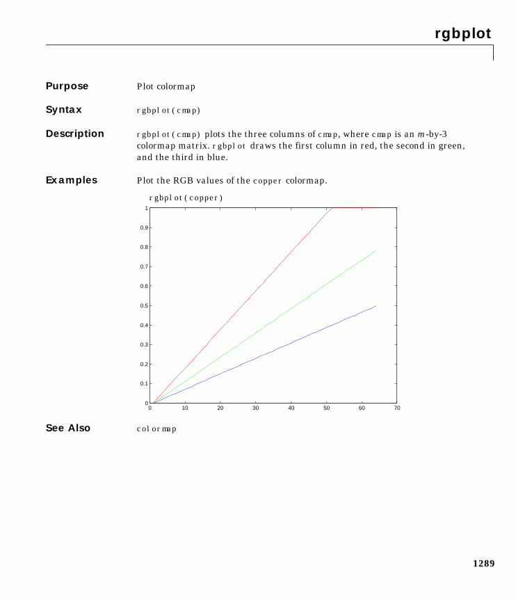
rgbplot
1289
1rgbplotPurpose Plot colormap
Syntax rgbplot(cmap)
Description rgbplot(cmap) plots the three columns of cmap, where cmap is an m-by-3colormap matrix. rgbplot draws the first column in red, the second in green,and the third in blue.
Examples Plot the RGB values of the copper colormap.
rgbplot(copper)
See Also colormap
0 10 20 30 40 50 60 700
0.1
0.2
0.3
0.4
0.5
0.6
0.7
0.8
0.9
1
ribbon
1290
1ribbonPurpose Ribbon plot
Syntax ribbon(Y)ribbon(X,Y)ribbon(X,Y,width)h = ribbon(...)
Description ribbon(Y) plots the columns of Y as separate three-dimensional ribbons usingX = 1:size(Y,1).
ribbon(X,Y) plots X versus the columns of Y as three-dimensional strips. X andY are vectors of the same size or matrices of the same size. Additionally, X canbe a row or a column vector, and Y a matrix with length(X) rows.
ribbon(X,Y,width) specifies the width of the ribbons. The default is 0.75.
h = ribbon(...) returns a vector of handles to surface graphics objects.ribbon returns one handle per strip.
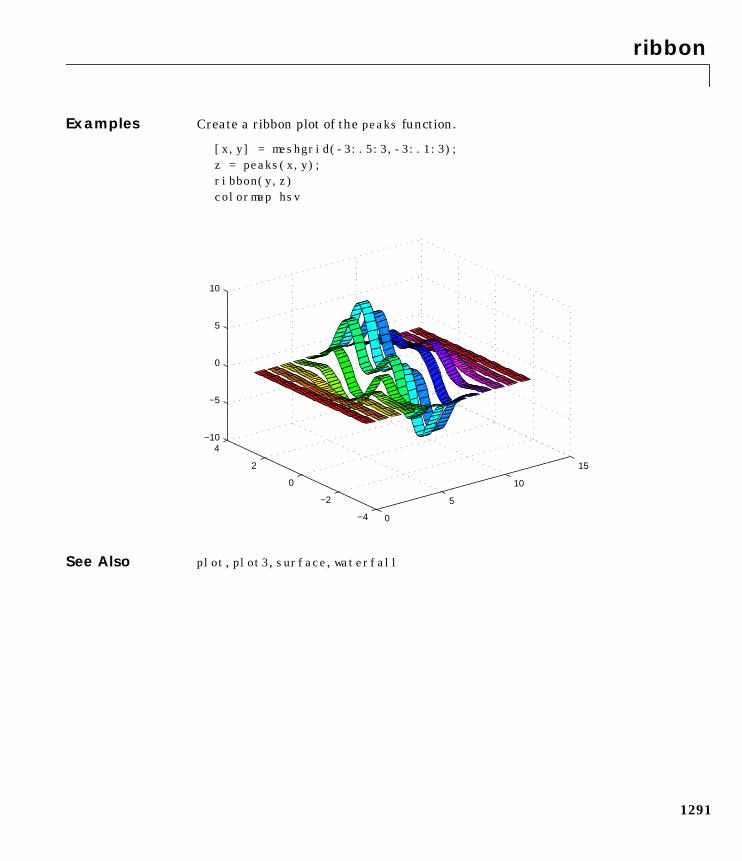
ribbon
1291
Examples Create a ribbon plot of the peaks function.
[x,y] = meshgrid(-3:.5:3,-3:.1:3);z = peaks(x,y);ribbon(y,z)colormap hsv
See Also plot, plot3, surface, waterfall
0
5
10
15
−4
−2
0
2
4−10
−5
0
5
10
rmappdata
1292
1rmappdataPurpose Remove application-defined data
Syntax rmappdata(h,name,value)
Description rmappdata(h,name,value) removes the application-defined data name fromthe object specified by handle h.
See Also getappdata, isappdata, setappdata
rmfield
1293
1rmfieldPurpose Remove structure fields
Syntax s = rmfield(s,'field')s = rmfield(s,FIELDS)
Description s = rmfield(s,'field') removes the specified field from the structure arrays.
s = rmfield(s,FIELDS) removes more than one field at a time when FIELDS isa character array of field names or cell array of strings.
See Also getfield, setfield, fieldnames
rmpath
1294
1rmpathPurpose Remove directories from the MATLAB search path
GraphicalInterface
As an alternative to the rmpath function, use the Set Path dialog box. To openit, select Set Path from the File menu in the MATLAB desktop.
Syntax rmpath('directory')rmpath directory
Description rmpath('directory') removes the specified directory from MATLAB’scurrent search path. Use the full pathname for directory.
rmpath directory is the unquoted form of the syntax.
Examples To remove /usr/local/matlab/mytools from the search path, type
rmpath /usr/local/matlab/mytools
See Also addpath, path, rehash, pathtoolr
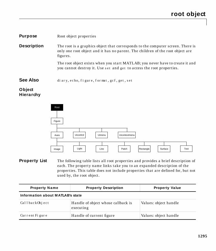
root object
1295
1root objectPurpose Root object properties
Description The root is a graphics object that corresponds to the computer screen. There isonly one root object and it has no parent. The children of the root object arefigures.
The root object exists when you start MATLAB; you never have to create it andyou cannot destroy it. Use set and get to access the root properties.
See Also diary, echo, figure, format, gcf, get, set
ObjectHierarchy
Property List The following table lists all root properties and provides a brief description ofeach. The property name links take you to an expanded description of theproperties. This table does not include properties that are defined for, but notused by, the root object.
Uimenu
Line
Axes Uicontrol
Image
Figure
Uicontextmenu
Light SurfacePatch Text
Root
Rectangle
Property Name Property Description Property Value
Information about MATLAB’s state
CallbackObject Handle of object whose callback isexecuting
Values: object handle
CurrentFigure Handle of current figure Values: object handle
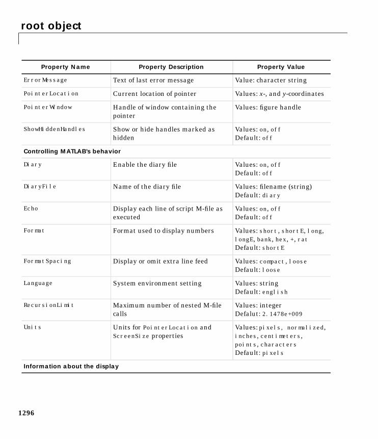
root object
1296
ErrorMessage Text of last error message Value: character string
PointerLocation Current location of pointer Values: x-, and y-coordinates
PointerWindow Handle of window containing thepointer
Values: figure handle
ShowHiddenHandles Show or hide handles marked ashidden
Values: on, offDefault: off
Controlling MATLAB’s behavior
Diary Enable the diary file Values: on, offDefault: off
DiaryFile Name of the diary file Values: filename (string)Default: diary
Echo Display each line of script M-file asexecuted
Values: on, offDefault: off
Format Format used to display numbers Values: short, shortE, long,longE, bank, hex, +, ratDefault: shortE
FormatSpacing Display or omit extra line feed Values: compact, looseDefault: loose
Language System environment setting Values: stringDefault: english
RecursionLimit Maximum number of nested M-filecalls
Values: integerDefalut: 2.1478e+009
Units Units for PointerLocation andScreenSize properties
Values: pixels, normalized,inches, centimeters,points, charactersDefault: pixels
Information about the display
Property Name Property Description Property Value
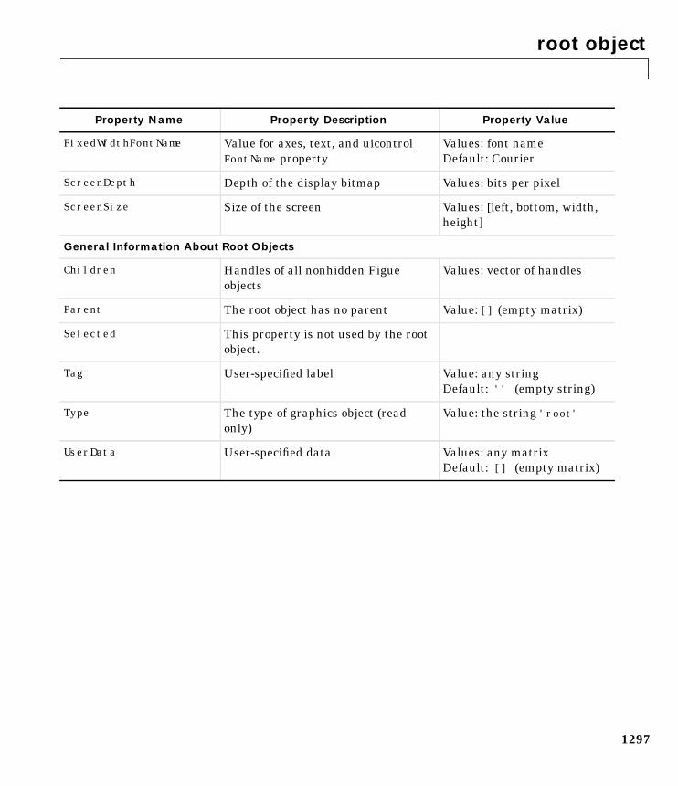
root object
1297
FixedWidthFontName Value for axes, text, and uicontrolFontName property
Values: font nameDefault: Courier
ScreenDepth Depth of the display bitmap Values: bits per pixel
ScreenSize Size of the screen Values: [left, bottom, width,height]
General Information About Root Objects
Children Handles of all nonhidden Figueobjects
Values: vector of handles
Parent The root object has no parent Value: [] (empty matrix)
Selected This property is not used by the rootobject.
Tag User-specified label Value: any stringDefault: '' (empty string)
Type The type of graphics object (readonly)
Value: the string 'root'
UserData User-specified data Values: any matrixDefault: [] (empty matrix)
Property Name Property Description Property Value
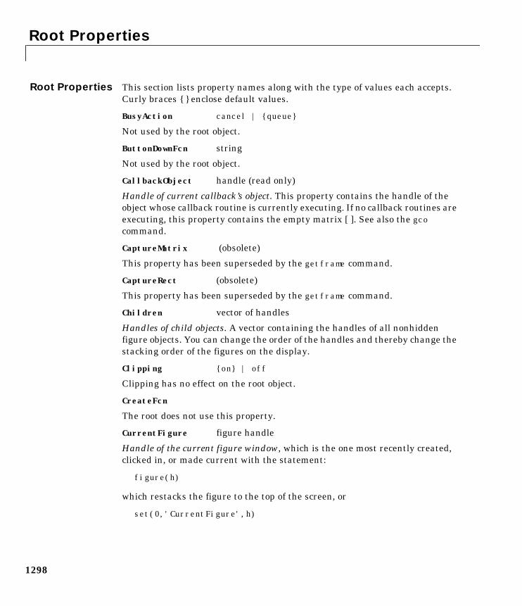
Root Properties
1298
1Root PropertiesRoot Properties This section lists property names along with the type of values each accepts.Curly braces enclose default values.
BusyAction cancel | queue
Not used by the root object.
ButtonDownFcn string
Not used by the root object.
CallbackObject handle (read only)
Handle of current callback’s object. This property contains the handle of theobject whose callback routine is currently executing. If no callback routines areexecuting, this property contains the empty matrix [ ]. See also the gcocommand.
CaptureMatrix (obsolete)
This property has been superseded by the getframe command.
CaptureRect (obsolete)
This property has been superseded by the getframe command.
Children vector of handles
Handles of child objects. A vector containing the handles of all nonhiddenfigure objects. You can change the order of the handles and thereby change thestacking order of the figures on the display.
Clipping on | off
Clipping has no effect on the root object.
CreateFcn
The root does not use this property.
CurrentFigure figure handle
Handle of the current figure window, which is the one most recently created,clicked in, or made current with the statement:
figure(h)
which restacks the figure to the top of the screen, or
set(0,'CurrentFigure',h)
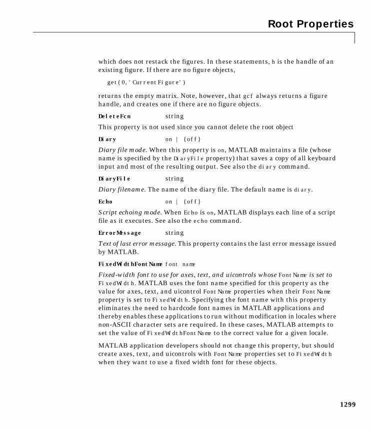
Root Properties
1299
which does not restack the figures. In these statements, h is the handle of anexisting figure. If there are no figure objects,
get(0,'CurrentFigure')
returns the empty matrix. Note, however, that gcf always returns a figurehandle, and creates one if there are no figure objects.
DeleteFcn string
This property is not used since you cannot delete the root object
Diary on | off
Diary file mode. When this property is on, MATLAB maintains a file (whosename is specified by the DiaryFile property) that saves a copy of all keyboardinput and most of the resulting output. See also the diary command.
DiaryFile string
Diary filename. The name of the diary file. The default name is diary.
Echo on | off
Script echoing mode. When Echo is on, MATLAB displays each line of a scriptfile as it executes. See also the echo command.
ErrorMessage string
Text of last error message. This property contains the last error message issuedby MATLAB.
FixedWidthFontName font name
Fixed-width font to use for axes, text, and uicontrols whose FontName is set toFixedWidth. MATLAB uses the font name specified for this property as thevalue for axes, text, and uicontrol FontName properties when their FontNameproperty is set to FixedWidth. Specifying the font name with this propertyeliminates the need to hardcode font names in MATLAB applications andthereby enables these applications to run without modification in locales wherenon-ASCII character sets are required. In these cases, MATLAB attempts toset the value of FixedWidthFontName to the correct value for a given locale.
MATLAB application developers should not change this property, but shouldcreate axes, text, and uicontrols with FontName properties set to FixedWidthwhen they want to use a fixed width font for these objects.
Root Properties
1300
MATLAB end users can set this property if they do not want to use thepreselected value. In locales where Latin-based characters are used, Courier isthe default.
Format short | shortE | long | longE | bank |hex | + | rat
Output format mode. This property sets the format used to display numbers.See also the format command.
• short – Fixed-point format with 5 digits.
• shortE – Floating-point format with 5 digits.
• shortG – Fixed- or floating-point format displaying as many significantfigures as possible with 5 digits.
• long – Scaled fixed-point format with 15 digits.
• longE – Floating-point format with 15 digits.
• longG – Fixed- or floating-point format displaying as many significant figuresas possible with 15 digits.
• bank – Fixed-format of dollars and cents.
• hex – Hexadecimal format.
• + – Displays + and – symbols.
• rat – Approximation by ratio of small integers.
FormatSpacing compact | loose
Output format spacing (see also format command).
• compact — Suppress extra line feeds for more compact display.
• loose — Display extra line feeds for a more readable display.
HandleVisibility on | callback | off
This property is not useful on the root object.
HitTest on | off
This property is not useful on the root object.
Interruptible on | off
This property is not useful on the root object.
Root Properties
1301
Language string
System environment setting.
Parent handle
Handle of parent object. This property always contains the empty matrix, asthe root object has no parent.
PointerLocation [x,y]
Current location of pointer. A vector containing the x- and y-coordinates of thepointer position, measured from the lower-left corner of the screen. You canmove the pointer by changing the values of this property. The Units propertydetermines the units of this measurement.
This property always contains the instantaneous pointer location, even if thepointer is not in a MATLAB window. A callback routine querying thePointerLocation can get a different value than the location of the pointer whenthe callback was triggered. This difference results from delays in callbackexecution caused by competition for system resources.
PointerWindow handle (read only)
Handle of window containing the pointer. MATLAB sets this property to thehandle of the figure window containing the pointer. If the pointer is not in aMATLAB window, the value of this property is 0. A callback routine queryingthe PointerWindow can get the wrong window handle if you move the pointer toanother window before the callback executes. This error results from delays incallback execution caused by competition for system resources.
RecursionLimit integer
Number of nested M-file calls. This property sets a limit to the number ofnested calls to M-files MATLAB will make before stoping (or potentiallyrunning out of memory). By default the value is set to a large value. Setting thisproperty to a smaller value (something like 150, for example) should preventMATLAB from running out of memory and will instead cause MATLAB toissue an error when the limit is reached.
ScreenDepth bits per pixel
Screen depth. The depth of the display bitmap (i.e., the number of bits perpixel). The maximum number of simultaneously displayed colors on thecurrent graphics device is 2 raised to this power.
Root Properties
1302
ScreenDepth supersedes the BlackAndWhite property. To override automatichardware checking, set this property to 1. This value causes MATLAB toassume the display is monochrome. This is useful if MATLAB is running oncolor hardware but is displaying on a monochrome terminal. Such a situationcan cause MATLAB to determine erroneously that the display is color.
ScreenSize 4-element rectangle vector (read only)
Screen size. A four-element vector,
[left,bottom,width,height]
that defines the display size. left and bottom are 0 for all Units except pixels,in which case left and bottom are 1. width and height are the screendimensions in units specified by the Units property.
Selected on | off
This property has no effect on the root level.
SelectionHighlight on | off
This property has no effect on the root level.
ShowHiddenHandles on | off
Show or hide handles marked as hidden. When set to on, this property disableshandle hiding and exposes all object handles, regardless of the setting of anobject’s HandleVisibility property. When set to off, all objects so markedremain hidden within the graphics hierarchy.
Tag string
User-specified object label. The Tag property provides a means to identifygraphics objects with a user-specified label. While it is not necessary to identifythe root object with a tag (since its handle is always 0), you can use thisproperty to store any string value that you can later retrieve using set.
Type string (read only)
Class of graphics object. For the root object, Type is always 'root'.
UIContextMenu handle
This property has no effect on the root level.
Root Properties
1303
Units pixels | normalized | inches | centimeters| points | characters
Unit of measurement. This property specifies the units MATLAB uses tointerpret size and location data. All units are measured from the lower-leftcorner of the screen. Normalized units map the lower-left corner of the screento (0,0) and the upper right corner to (1.0,1.0). inches, centimeters, and pointsare absolute units (one point equals 1/72 of an inch). Characters are unitsdefined by characters from the default system font; the width of one unit is thewidth of the letter x, the height of one character is the distance between thebaselines of two lines of text.
This property affects the PointerLocation and ScreenSize properties. If youchange the value of Units, it is good practice to return it to its default valueafter completing your operation so as not to affect other functions that assumeUnits is set to the default value.
UserData matrix
User specified data. This property can be any data you want to associate withthe root object. MATLAB does not use this property, but you can access it usingthe set and get functions.
Visible on | off
Object visibility. This property has no effect on the root object.
roots
1304
1rootsPurpose Polynomial roots
Syntax r = roots(c)
Description r = roots(c) returns a column vector whose elements are the roots of thepolynomial c.
Row vector c contains the coefficients of a polynomial, ordered in descendingpowers. If c has n+1 components, the polynomial it represents is
.
Remarks Note the relationship of this function to p = poly(r), which returns a rowvector whose elements are the coefficients of the polynomial. For vectors, rootsand poly are inverse functions of each other, up to ordering, scaling, androundoff error.
Examples The polynomial is represented in MATLAB as
p = [1 -6 -72 -27]
The roots of this polynomial are returned in a column vector by
r = roots(p)r = 12.1229 -5.7345 -0.3884
Algorithm The algorithm simply involves computing the eigenvalues of the companionmatrix:
A = diag(ones(n-2,1),-1);A(1,:) = -c(2:n-1)./c(1);eig(A)
It is possible to prove that the results produced are the exact eigenvalues of amatrix within roundoff error of the companion matrix A, but this does not meanthat they are the exact roots of a polynomial with coefficients within roundofferror of those in c.
c1sn … cns cn 1++ + +
s3 6s2– 72s– 27–

roots
1305
See Also fzero, poly, residue
rose
1306
1rosePurpose Angle histogram
Syntax rose(theta)rose(theta,x)rose(theta,nbins)[tout,rout] = rose(...)
Description rose creates an angle histogram, which is a polar plot showing the distributionof values grouped according to their numeric range. Each group is shown as onebin.
rose(theta) plots an angle histogram showing the distribution of theta in 20angle bins or less. The vector theta, expressed in radians, determines the anglefrom the origin of each bin. The length of each bin reflects the number ofelements in theta that fall within a group, which ranges from 0 to the greatestnumber of elements deposited in any one bin.
rose(theta,x) uses the vector x to specify the number and the locations ofbins. length(x) is the number of bins and the values of x specify the centerangle of each bin. For example, if x is a five-element vector, rose distributes theelements of theta in five bins centered at the specified x values.
rose(theta,nbins) plots nbins equally spaced bins in the range [0, 2*pi].The default is 20.
[tout,rout] = rose(...) returns the vectors tout and rout sopolar(tout,rout) generates the histogram for the data. This syntax does notgenerate a plot.
Example Create a rose plot showing the distribution of 50 random numbers.
theta = 2*pi*rand(1,50);rose(theta)
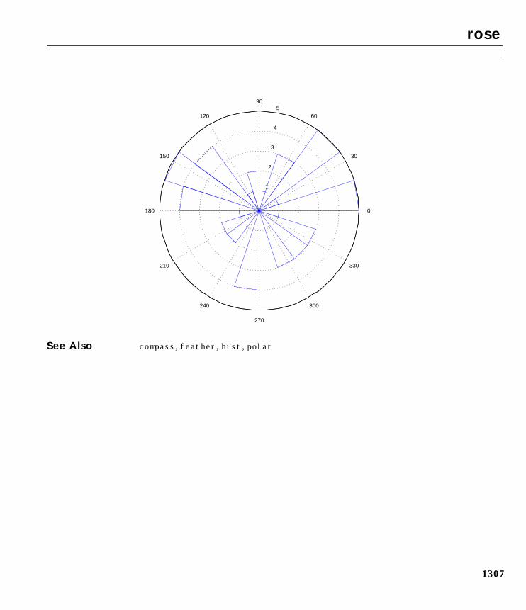
rose
1307
See Also compass, feather, hist, polar
1
2
3
4
5
30
210
60
240
90
270
120
300
150
330
180 0
rot90
1308
1rot90Purpose Rotate matrix 90˚
Syntax B = rot90(A)B = rot90(A,k)
Description B = rot90(A) rotates matrix A counterclockwise by 90 degrees.
B = rot90(A,k) rotates matrix A counterclockwise by k∗90 degrees, where k isan integer.
Examples The matrix
X = 1 2 3 4 5 6 7 8 9
rotated by 90 degrees is
Y = rot90(X)Y = 3 6 9 2 5 8 1 4 7
See Also flipdim, fliplr, flipud
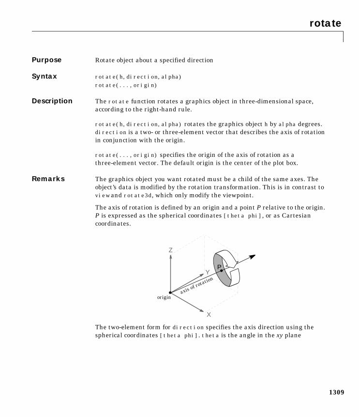
rotate
1309
1rotatePurpose Rotate object about a specified direction
Syntax rotate(h,direction,alpha)rotate(...,origin)
Description The rotate function rotates a graphics object in three-dimensional space,according to the right-hand rule.
rotate(h,direction,alpha) rotates the graphics object h by alpha degrees.direction is a two- or three-element vector that describes the axis of rotationin conjunction with the origin.
rotate(...,origin) specifies the origin of the axis of rotation as athree-element vector. The default origin is the center of the plot box.
Remarks The graphics object you want rotated must be a child of the same axes. Theobject’s data is modified by the rotation transformation. This is in contrast toview and rotate3d, which only modify the viewpoint.
The axis of rotation is defined by an origin and a point P relative to the origin.P is expressed as the spherical coordinates [theta phi], or as Cartesiancoordinates.
The two-element form for direction specifies the axis direction using thespherical coordinates [theta phi]. theta is the angle in the xy plane
Z
Y
X
P
originaxis of ro
tation
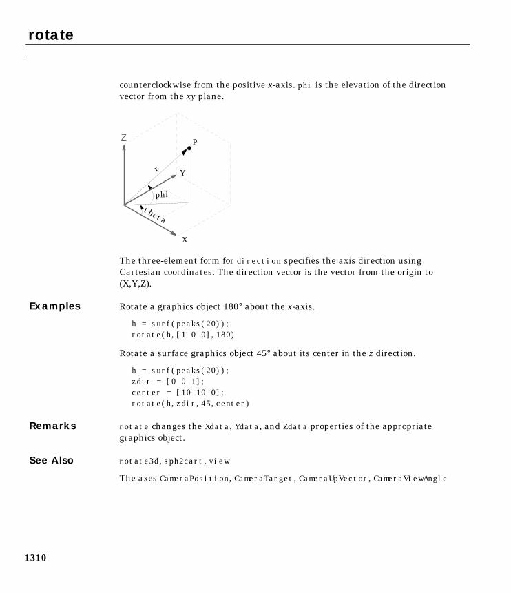
rotate
1310
counterclockwise from the positive x-axis. phi is the elevation of the directionvector from the xy plane.
The three-element form for direction specifies the axis direction usingCartesian coordinates. The direction vector is the vector from the origin to(X,Y,Z).
Examples Rotate a graphics object 180° about the x-axis.
h = surf(peaks(20));rotate(h,[1 0 0],180)
Rotate a surface graphics object 45° about its center in the z direction.
h = surf(peaks(20));zdir = [0 0 1];center = [10 10 0];rotate(h,zdir,45,center)
Remarks rotate changes the Xdata, Ydata, and Zdata properties of the appropriategraphics object.
See Also rotate3d, sph2cart, view
The axes CameraPosition, CameraTarget, CameraUpVector, CameraViewAngle
Z
Y
X
theta
P
phi
r
rotate3d
1311
1rotate3dPurpose Rotate axes using mouse
Syntax rotate3drotate3d onrotate3d off
Description rotate3d on enables interactive axes rotation within the current figure usingthe mouse. When interactive axes rotation is enabled, clicking on an axesdraws an animated box, which rotates as the mouse is dragged, showing theview that will result when the mouse button is released. A numeric readoutappears in the lower-left corner of the figure during this time, showing thecurrent azimuth and elevation of the animated box. Releasing the mousebutton removes the animated box and the readout, and changes the view of theaxes to correspond to the last orientation of the animated box.
rotate3d off disables interactive axes rotation in the current figure.
rotate3d toggles interactive axes rotation in the current figure.
Double clicking on the figure restores the original view.
See Also camorbit, rotate, view
round
1312
1roundPurpose Round to nearest integer
Syntax Y = round(X)
Description Y = round(X) rounds the elements of X to the nearest integers. For complex X,the imaginary and real parts are rounded independently.
Examples a = [-1.9, -0.2, 3.4, 5.6, 7.0, 2.4+3.6i]
a = Columns 1 through 4-1.9000 -0.2000 3.4000 5.6000
Columns 5 through 6 7.0000 2.4000 + 3.6000i
round(a)
ans = Columns 1 through 4-2.0000 0 3.0000 6.0000
Columns 5 through 6 7.0000 2.0000 + 4.0000i
See Also ceil, fix, floor
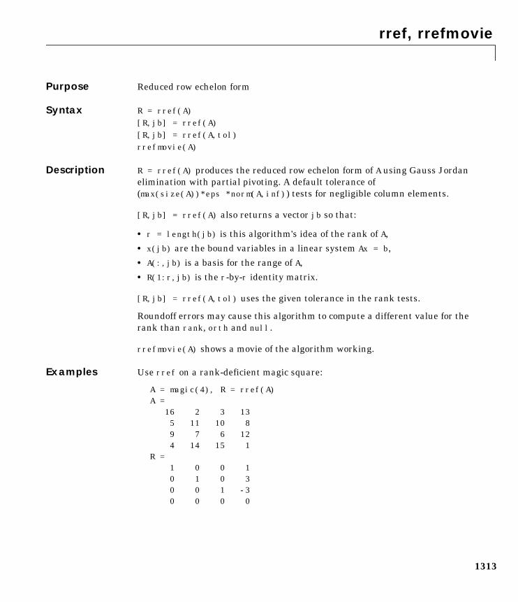
rref, rrefmovie
1313
1rref, rrefmoviePurpose Reduced row echelon form
Syntax R = rref(A)[R,jb] = rref(A)[R,jb] = rref(A,tol)rrefmovie(A)
Description R = rref(A) produces the reduced row echelon form of A using Gauss Jordanelimination with partial pivoting. A default tolerance of(max(size(A))*eps *norm(A,inf)) tests for negligible column elements.
[R,jb] = rref(A) also returns a vector jb so that:
• r = length(jb) is this algorithm's idea of the rank of A,
• x(jb) are the bound variables in a linear system Ax = b,
• A(:,jb) is a basis for the range of A,
• R(1:r,jb) is the r-by-r identity matrix.
[R,jb] = rref(A,tol) uses the given tolerance in the rank tests.
Roundoff errors may cause this algorithm to compute a different value for therank than rank, orth and null.
rrefmovie(A) shows a movie of the algorithm working.
Examples Use rref on a rank-deficient magic square:
A = magic(4), R = rref(A)A = 16 2 3 13 5 11 10 8 9 7 6 12 4 14 15 1R = 1 0 0 1 0 1 0 3 0 0 1 -3 0 0 0 0

rref, rrefmovie
1314
See Also inv, lu, rank
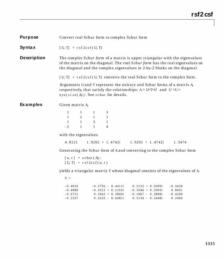
rsf2csf
1315
1rsf2csfPurpose Convert real Schur form to complex Schur form
Syntax [U,T] = rsf2csf(U,T)
Description The complex Schur form of a matrix is upper triangular with the eigenvaluesof the matrix on the diagonal. The real Schur form has the real eigenvalues onthe diagonal and the complex eigenvalues in 2-by-2 blocks on the diagonal.
[U,T] = rsf2csf(U,T) converts the real Schur form to the complex form.
Arguments U and T represent the unitary and Schur forms of a matrix A,respectively, that satisfy the relationships: A = U∗T∗U' and U'∗U =eye(size(A)). See schur for details.
Examples Given matrix A,
1 1 1 3 1 2 1 1 1 1 3 1-2 1 1 4
with the eigenvalues
4.8121 1.9202 + 1.4742i 1.9202 + 1.4742i 1.3474
Generating the Schur form of A and converting to the complex Schur form
[u,t] = schur(A);[U,T] = rsf2csf(u,t)
yields a triangular matrix T whose diagonal consists of the eigenvalues of A.
U =
-0.4916 -0.2756 - 0.4411i 0.2133 + 0.5699i -0.3428-0.4980 -0.1012 + 0.2163i -0.1046 + 0.2093i 0.8001-0.6751 0.1842 + 0.3860i -0.1867 - 0.3808i -0.4260-0.2337 0.2635 - 0.6481i 0.3134 - 0.5448i 0.2466
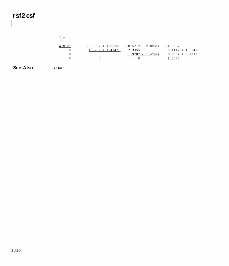
rsf2csf
1316
T =
4.8121 -0.9697 + 1.0778i -0.5212 + 2.0051i -1.0067 0 1.9202 + 1.4742i 2.3355 0.1117 + 1.6547i 0 0 1.9202 - 1.4742i 0.8002 + 0.2310i 0 0 0 1.3474
See Also schur

rsf2csf
1317
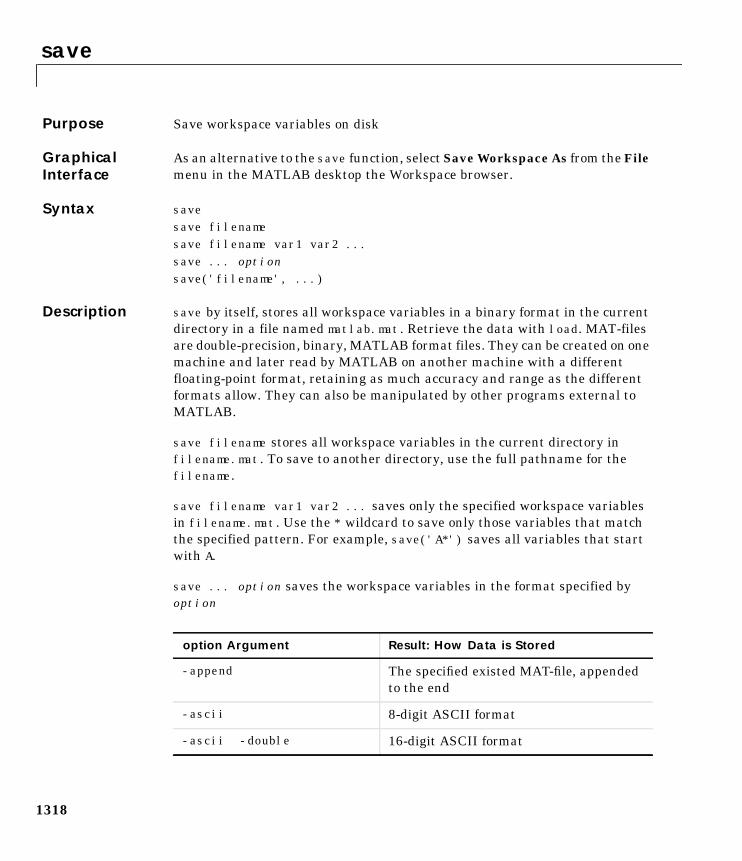
save
1318
1savePurpose Save workspace variables on disk
GraphicalInterface
As an alternative to the save function, select Save Workspace As from the Filemenu in the MATLAB desktop the Workspace browser.
Syntax savesave filenamesave filename var1 var2 ...save ... optionsave('filename', ...)
Description save by itself, stores all workspace variables in a binary format in the currentdirectory in a file named matlab.mat. Retrieve the data with load. MAT-filesare double-precision, binary, MATLAB format files. They can be created on onemachine and later read by MATLAB on another machine with a differentfloating-point format, retaining as much accuracy and range as the differentformats allow. They can also be manipulated by other programs external toMATLAB.
save filename stores all workspace variables in the current directory infilename.mat. To save to another directory, use the full pathname for thefilename.
save filename var1 var2 ... saves only the specified workspace variablesin filename.mat. Use the * wildcard to save only those variables that matchthe specified pattern. For example, save('A*') saves all variables that startwith A.
save ... option saves the workspace variables in the format specified byoption
option Argument Result: How Data is Stored
-append The specified existed MAT-file, appendedto the end
-ascii 8-digit ASCII format
-ascii -double 16-digit ASCII format
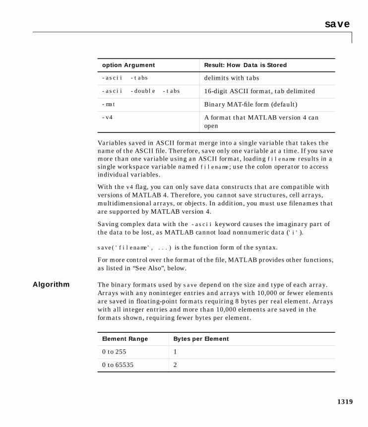
save
1319
Variables saved in ASCII format merge into a single variable that takes thename of the ASCII file. Therefore, save only one variable at a time. If you savemore than one variable using an ASCII format, loading filename results in asingle workspace variable named filename; use the colon operator to accessindividual variables.
With the v4 flag, you can only save data constructs that are compatible withversions of MATLAB 4. Therefore, you cannot save structures, cell arrays,multidimensional arrays, or objects. In addition, you must use filenames thatare supported by MATLAB version 4.
Saving complex data with the -ascii keyword causes the imaginary part ofthe data to be lost, as MATLAB cannot load nonnumeric data ('i').
save('filename', ...) is the function form of the syntax.
For more control over the format of the file, MATLAB provides other functions,as listed in “See Also”, below.
Algorithm The binary formats used by save depend on the size and type of each array.Arrays with any noninteger entries and arrays with 10,000 or fewer elementsare saved in floating-point formats requiring 8 bytes per real element. Arrayswith all integer entries and more than 10,000 elements are saved in theformats shown, requiring fewer bytes per element.
-ascii -tabs delimits with tabs
-ascii -double -tabs 16-digit ASCII format, tab delimited
-mat Binary MAT-file form (default)
-v4 A format that MATLAB version 4 canopen
option Argument Result: How Data is Stored
Element Range Bytes per Element
0 to 255 1
0 to 65535 2
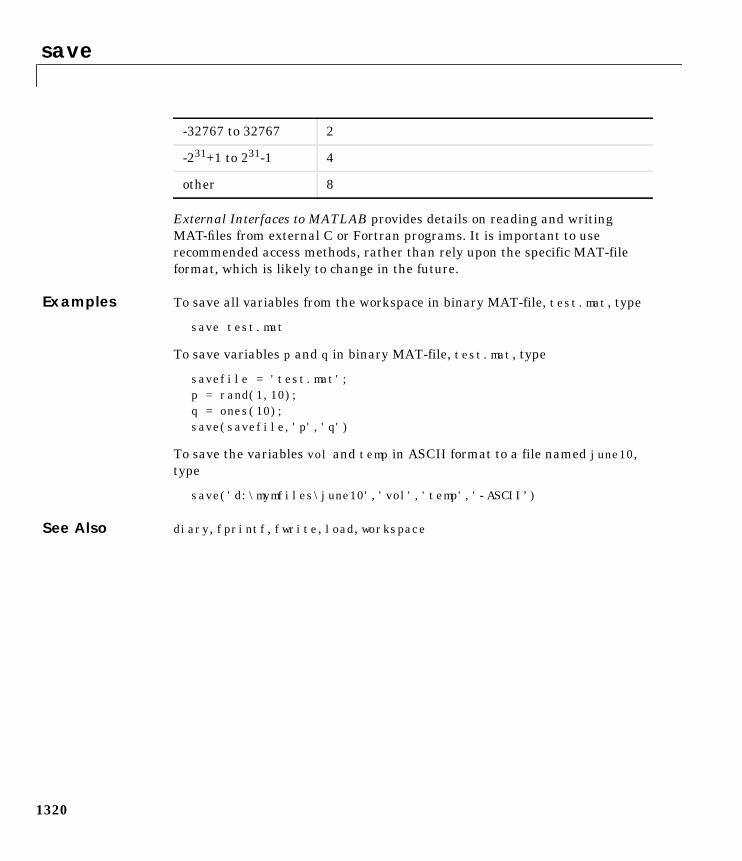
save
1320
External Interfaces to MATLAB provides details on reading and writingMAT-files from external C or Fortran programs. It is important to userecommended access methods, rather than rely upon the specific MAT-fileformat, which is likely to change in the future.
Examples To save all variables from the workspace in binary MAT-file, test.mat, type
save test.mat
To save variables p and q in binary MAT-file, test.mat, type
savefile = 'test.mat';p = rand(1,10);q = ones(10);save(savefile,'p','q')
To save the variables vol and temp in ASCII format to a file named june10,type
save('d:\mymfiles\june10','vol','temp','-ASCII’)
See Also diary, fprintf, fwrite, load, workspace
-32767 to 32767 2
-231+1 to 231-1 4
other 8
save (serial)
1321
1save (serial)Purpose Save serial port objects and variables to a MAT-file
Syntax save filenamesave filename obj1 obj2...
Arguments
Description save filename saves all MATLAB variables to the MAT-file filename. If anextension is not specified for filename, then the .mat extension is used.
save filename obj1 obj2... saves the serial port objects obj1 obj2 ... to theMAT-file filename.
Remarks You can use save in the functional form as well as the command form shownabove. When using the functional form, you must specify the filename andserial port objects as strings. For example. to save the serial port object s to thefile MySerial.mat
s = serial('COM1');save('MySerial','s')
Any data that is associated with the serial port object is not automaticallystored in the MAT-file. For example, suppose there is data in the input bufferfor obj. To save that data to a MAT-file, you must bring it into the MATLABworkspace using one of the synchronous read functions, and then save to theMAT-file using a separate variable name. You can also save data to a text filewith the record function.
You return objects and variables to the MATLAB workspace with the loadcommand. Values for read-only properties are restored to their default valuesupon loading. For example, the Status property is restored to closed. Todetermine if a property is read-only, examine its reference pages.
If you use the help command to display help for save, then you need to supplythe pathname shown below.
help serial/private/save
Example This example illustrates how to use the command and functional form of save.
filename The MAT-file name.
obj1 obj2... Serial port objects or arrays of serial port objects.
save (serial)
1322
s = serial('COM1');set(s,'BaudRate',2400,'StopBits',1)save MySerial1 sset(s,'BytesAvailableAction','MyAction')save('MySerial2','s')
See Also Functionsload, record
PropertiesStatus
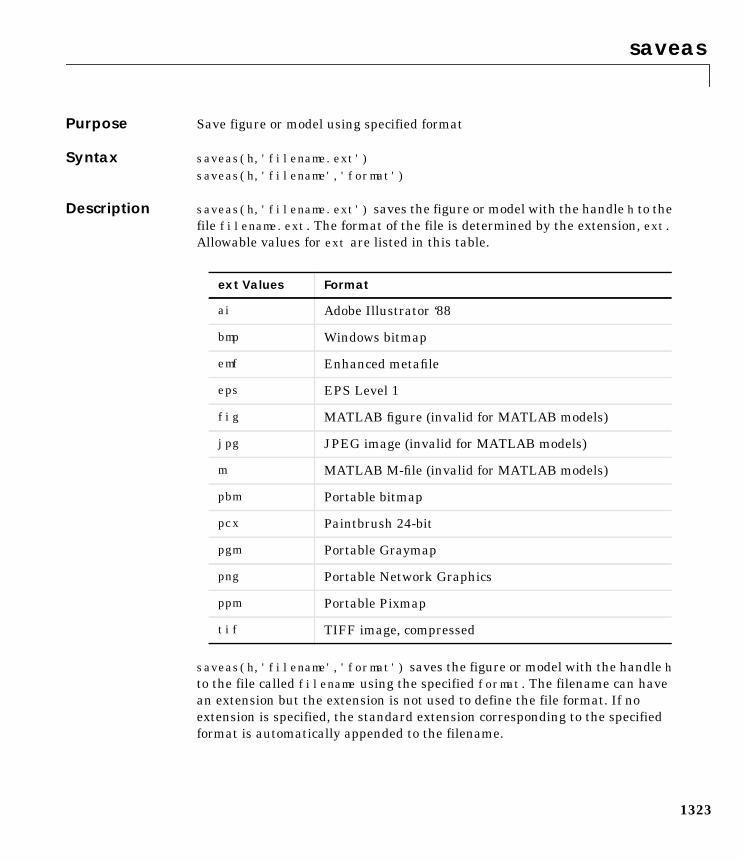
saveas
1323
1saveasPurpose Save figure or model using specified format
Syntax saveas(h,'filename.ext')saveas(h,'filename','format')
Description saveas(h,'filename.ext') saves the figure or model with the handle h to thefile filename.ext. The format of the file is determined by the extension, ext.Allowable values for ext are listed in this table.
saveas(h,'filename','format') saves the figure or model with the handle hto the file called filename using the specified format. The filename can havean extension but the extension is not used to define the file format. If noextension is specified, the standard extension corresponding to the specifiedformat is automatically appended to the filename.
ext Values Format
ai Adobe Illustrator ‘88
bmp Windows bitmap
emf Enhanced metafile
eps EPS Level 1
fig MATLAB figure (invalid for MATLAB models)
jpg JPEG image (invalid for MATLAB models)
m MATLAB M-file (invalid for MATLAB models)
pbm Portable bitmap
pcx Paintbrush 24-bit
pgm Portable Graymap
png Portable Network Graphics
ppm Portable Pixmap
tif TIFF image, compressed
saveas
1324
Allowable values for format are the extensions in the table above and thedevice types supported by print. The print device types include the formatslisted in the table of extensions above as well as additional file formats. Use anextension from the table above or from the list of device types supported byprint. When using the print device type to specify format for saveas, do notuse the prepended -d.
Remarks You can use open to open files saved using saveas with an m or fig extension.Other formats are not supported by open. The Save As dialog box you accessfrom the figure window’s File menu uses saveas, limiting the file extensions tom and fig. The Export dialog box you access from the figure window’s Filemenu uses saveas with the format argument.
Examples Example 1 – Specify File ExtensionSave the current figure that you annotated using the Plot Editor to a file namedpred_prey using the MATLAB fig format. This allows you to open the filepred_prey.fig at a later time and continue editing it with the Plot Editor.
saveas(gcf,'pred_prey.fig')
Example 2 – Specify File Format but No ExtensionSave the current figure, using Adobe Illustrator format, to the file logo. Usethe ai extension from the above table to specify the format. The file created islogo.ai.
saveas(gcf,'logo', 'ai')
This is the same as using the Adobe Illustrator format from the print devicestable, which is -dill; use doc print or help print to see the table for printdevice types. The file created is logo.ai. MATLAB automatically appends theai extension, for an Illustrator format file, because no extension was specified.
saveas(gcf,'logo', 'ill')
Example 3 – Specify File Format and ExtensionSave the current figure to the file star.eps using the Level 2 Color PostScriptformat. If you use doc print or help print, you can see from the table for print
saveas
1325
device types that the device type for this format is -dpsc2. The file created isstar.eps.
saveas(gcf,'star.eps', 'psc2')
In another example, save the current model to the file trans.tiff using theTIFF format with no compression. From the table for print device types, youcan see the device type for this format is -dtiffn. The file created istrans.tiff.
saveas(gcf,'trans.tiff', 'tiffn')
See Also open, print
saveobj
1326
1saveobjPurpose Save an object to a MAT-file
Syntax B = saveobj(A)
Description B = saveobj(A) is called by the MATLAB save function when object, A, issaved to a .MAT file. This call executes the saveobj method for the object’sclass, if such a method exists. The return value B is subsequently used by saveto populate the .MAT file.
When you issue a save command on an object, MATLAB looks for a methodcalled saveobj in the class directory. You can overload this method to modifythe object before the save operation. For example, you could define a saveobjmethod that saves related data along with the object.
saveobj will be separately invoked for each object to be saved.
saveobj can be overloaded only for user objects. save will not call saveobj fora built-in datatype, such as double, even if @double/saveobj exists.
Examples The following example shows a saveobj method written for the portfolioclass. The method determines if a portfolio object has already been assignedan account number from a previous save operation. If not, saveobj callsgetAccountNumber to obtain the number and assigns it to the account_numberfield. The contents of b is saved to the MAT-file.
function b = saveobj(a)if isempty(a.account_number) a.account_number = getAccountNumber(a);endb = a;
See Also save, loadobj
scatter
1327
1scatterPurpose 2-D Scatter plot
Syntax scatter(X,Y,S,C)scatter(X,Y)scatter(X,Y,S)scatter(...,markertype)scatter(...,'filled')h = scatter(...,)
Description scatter(X,Y,S,C) displays colored circles at the locations specified by thevectors X and Y (which must be the same size).
S determines the area of each marker (specified in points^2). S can be a vectorthe same length as X and Y or a scalar. If S is a scalar, MATLAB draws all themarkers the same size.
C determines the colors of each marker. When C is a vector the same length asX and Y, the values in C are linearly mapped to the colors in the currentcolormap. When C is a length(X)-by-3 matrix, it specifies the colors of themarkers as RGB values. C can also be a color string (see ColorSpec for a list ofcolor string specifiers)
scatter(X,Y) draws the markers in the default size and color.
scatter(X,Y,S) draws the markers at the specified sizes (S) with a singlecolor.
scatter(...,markertype) uses the marker type specified instead of 'o' (seeLineSpec for a list of marker specifiers).
scatter(...,'filled') fills the markers.
h = scatter(...) returns the handles to the line objects created by scatter(see line for a list of properties you can specify using the object handles andset).
Remarks Use plot for single color, single marker size scatter plots.
Examples load seamountscatter(x,y,5,z)
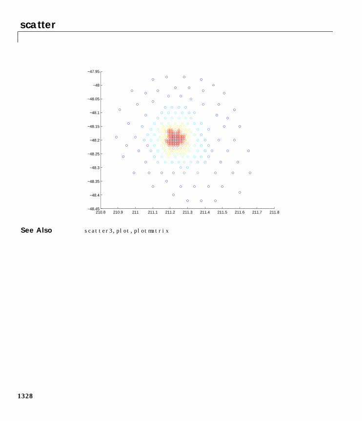
scatter
1328
See Also scatter3, plot, plotmatrix
210.8 210.9 211 211.1 211.2 211.3 211.4 211.5 211.6 211.7 211.8−48.45
−48.4
−48.35
−48.3
−48.25
−48.2
−48.15
−48.1
−48.05
−48
−47.95
scatter3
1329
1scatter3Purpose 3-D scatter plot
Syntax scatter3(X,Y,Z,S,C)scatter3(X,Y,Z)scatter3(X,Y,Z,S)scatter3(...,markertype)scatter3(...,'filled')h = scatter3(...,)
Description scatter3(X,Y,Z,S,C) displays colored circles at the locations specified by thevectors X, Y, and Z (which must all be the same size).
S determines the size of each marker (specified in points). S can be a vector thesame length as X, Y, and Z or a scalar. If S is a scalar, MATLAB draws all themarkers the same size.
C determines the colors of each marker. When C is a vector the same length asX, Y, and Z, the values in C are linearly mapped to the colors in the currentcolormap. When C is a length(X)-by-3 matrix, it specifies the colors of themarkers as RGB values. C can also be a color string (see ColorSpec for a list ofcolor string specifiers)
scatter3(X,Y,Z) draws the markers in the default size and color.
scatter3(X,Y,Z,S) draws the markers at the specified sizes (S) with a singlecolor.
scatter3(...,markertype) uses the marker type specified instead of 'o' (seeLineSpec for a list of marker specifiers).
scatter3(...,'filled') fills the markers.
h = scatter3(...) returns the handles to the line objects created by scatter3(see line for a list of properties you can specify using the object handles andset).
Remarks Use plot3 for single color, single marker size 3-D scatter plots.
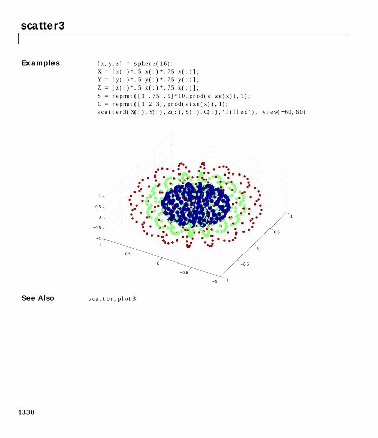
scatter3
1330
Examples [x,y,z] = sphere(16);X = [x(:)*.5 x(:)*.75 x(:)];Y = [y(:)*.5 y(:)*.75 y(:)];Z = [z(:)*.5 z(:)*.75 z(:)];S = repmat([1 .75 .5]*10,prod(size(x)),1);C = repmat([1 2 3],prod(size(x)),1);scatter3(X(:),Y(:),Z(:),S(:),C(:),’filled’), view(−60,60)
See Also scatter, plot3
−1
−0.5
0
0.5
1
−1
−0.5
0
0.5
1
−1
−0.5
0
0.5
1
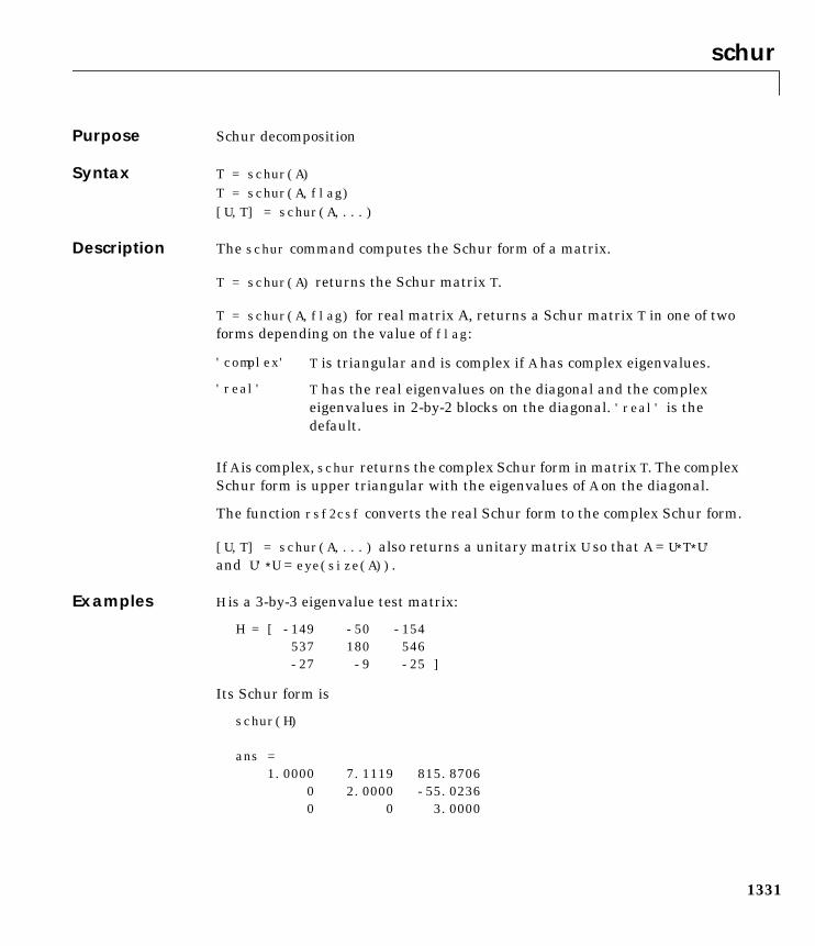
schur
1331
1schurPurpose Schur decomposition
Syntax T = schur(A)T = schur(A,flag)[U,T] = schur(A,...)
Description The schur command computes the Schur form of a matrix.
T = schur(A) returns the Schur matrix T.
T = schur(A,flag) for real matrix A, returns a Schur matrix T in one of twoforms depending on the value of flag:
If A is complex, schur returns the complex Schur form in matrix T. The complexSchur form is upper triangular with the eigenvalues of A on the diagonal.
The function rsf2csf converts the real Schur form to the complex Schur form.
[U,T] = schur(A,...) also returns a unitary matrix U so that A = U∗T∗U'and U'∗U = eye(size(A)).
Examples H is a 3-by-3 eigenvalue test matrix:
H = [ -149 -50 -154537 180 546
-27 -9 -25 ]
Its Schur form is
schur(H)
ans =1.0000 7.1119 815.8706
0 2.0000 -55.02360 0 3.0000
'complex' T is triangular and is complex if A has complex eigenvalues.
'real' T has the real eigenvalues on the diagonal and the complexeigenvalues in 2-by-2 blocks on the diagonal. 'real' is thedefault.
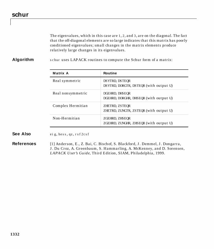
schur
1332
The eigenvalues, which in this case are 1, 2, and 3, are on the diagonal. The factthat the off-diagonal elements are so large indicates that this matrix has poorlyconditioned eigenvalues; small changes in the matrix elements producerelatively large changes in its eigenvalues.
Algorithm schur uses LAPACK routines to compute the Schur form of a matrix:
See Also eig, hess, qz, rsf2csf
References [1] Anderson, E., Z. Bai, C. Bischof, S. Blackford, J. Demmel, J. Dongarra,J. Du Croz, A. Greenbaum, S. Hammarling, A. McKenney, and D. Sorensen,LAPACK User’s Guide, Third Edition, SIAM, Philadelphia, 1999.
Matrix A Routine
Real symmetric DSYTRD, DSTEQRDSYTRD, DORGTR, DSTEQR (with output U)
Real nonsymmetric DGEHRD, DHSEQRDGEHRD, DORGHR, DHSEQR (with output U)
Complex Hermitian ZHETRD, ZSTEQRZHETRD, ZUNGTR, ZSTEQR (with output U)
Non-Hermitian ZGEHRD, ZHSEQRZGEHRD, ZUNGHR, ZHSEQR (with output U)
script
1333
1scriptPurpose Script M-files
Description A script file is an external file that contains a sequence of MATLABstatements. By typing the filename, subsequent MATLAB input is obtainedfrom the file. Script files have a filename extension of .m and are often calledM-files.
Scripts are the simplest kind of M-file. They are useful for automating blocksof MATLAB commands, such as computations you have to perform repeatedlyfrom the command line. Scripts can operate on existing data in the workspace,or they can create new data on which to operate. Although scripts do not returnoutput arguments, any variables that they create remain in the workspace soyou can use them in further computations. In addition, scripts can producegraphical output using commands like plot.
Scripts can contain any series of MATLAB statements. They require nodeclarations or begin/end delimiters.
Like any M-file, scripts can contain comments. Any text following a percentsign (%) on a given line is comment text. Comments can appear on lines bythemselves, or you can append them to the end of any executable line.
See Also echo Echo M-files during executionfunction Function M-filestype List file
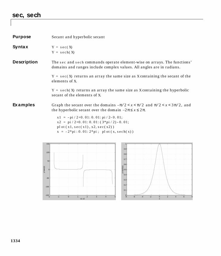
sec, sech
1334
1sec, sechPurpose Secant and hyperbolic secant
Syntax Y = sec(X)Y = sech(X)
Description The sec and sech commands operate element-wise on arrays. The functions’domains and ranges include complex values. All angles are in radians.
Y = sec(X) returns an array the same size as X containing the secant of theelements of X.
Y = sech(X) returns an array the same size as X containing the hyperbolicsecant of the elements of X.
Examples Graph the secant over the domains and andthe hyperbolic secant over the domain
x1 = -pi/2+0.01:0.01:pi/2-0.01;x2 = pi/2+0.01:0.01:(3*pi/2)-0.01;plot(x1,sec(x1),x2,sec(x2))x = -2*pi:0.01:2*pi; plot(x,sech(x))
π– 2⁄ x π 2⁄< < π 2⁄ x 3π 2⁄ ,< <2π– x 2π.≤ ≤
-8 -6 -4 -2 0 2 4 6 80
0.1
0.2
0.3
0.4
0.5
0.6
0.7
0.8
0.9
1
x
y=se
ch(x
)
-2 -1 0 1 2 3 4 5-150
-100
-50
0
50
100
150
x1 x2
y=se
c(x)
sec, sech
1335
The expression sec(pi/2) does not evaluate as infinite but as the reciprocal ofthe floating-point accuracy eps, because pi is a floating-point approximation tothe exact value of π.
Algorithm
See Also asec, asech Inverse secant and inverse hyperbolic secant
z( )sec 1z( )cos
----------------- z( )sech 1z( )cosh
--------------------==
selectmoveresize
1336
1selectmoveresizePurpose Select, move, resize, or copy axes and uicontrol graphics objects
Syntax A = selectmoveresize;set(h,'ButtonDownFcn','selectmoveresize')
Description selectmoveresize is useful as the callback routine for axes and uicontrolbutton down functions. When executed, it selects the object and allows you tomove, resize, and copy it.
For example, this statement sets the ButtonDownFcn of the current axes toselectmoveresize:
set(gca,'ButtonDownFcn','selectmoveresize')
A = selectmoveresize returns a structure array containing:
• A.Type: a string containing the action type, which can be Select, Move,Resize, or Copy.
• A.Handles: a list of the selected handles or for a Copy an m-by-2 matrixcontaining the original handles in the first column and the new handles inthe second column.
See Also The ButtonDownFcn of axes and uicontrol graphics objects
semilogx, semilogy
1337
1semilogx, semilogyPurpose Semi-logarithmic plots
Syntax semilogx(Y)semilogx(X1,Y1,...)semilogx(X1,Y1,LineSpec,...)semilogx(...,'PropertyName',PropertyValue,...)h = semilogx(...)
semilogy(...)h = semilogy(...)
Description semilogx and semilogy plot data as logarithmic scales for the x- and y-axis,respectively. logarithmic
semilogx(Y) creates a plot using a base 10 logarithmic scale for the x-axis anda linear scale for the y-axis. It plots the columns of Y versus their index if Ycontains real numbers. semilogx(Y) is equivalent to semilogx(real(Y),imag(Y)) if Y contains complex numbers. semilogx ignores the imaginarycomponent in all other uses of this function.
semilogx(X1,Y1,...) plots all Xn versus Yn pairs. If only Xn or Yn is a matrix,semilogx plots the vector argument versus the rows or columns of the matrix,depending on whether the vector’s row or column dimension matches thematrix.
semilogx(X1,Y1,LineSpec,...) plots all lines defined by the Xn,Yn,LineSpectriples. LineSpec determines line style, marker symbol, and color of the plottedlines.
semilogx(...,'PropertyName',PropertyValue,...) sets property values forall line graphics objects created by semilogx.
semilogy(...) creates a plot using a base 10 logarithmic scale for the y-axisand a linear scale for the x-axis.
h = semilogx(...) and h = semilogy(...) return a vector of handles to linegraphics objects, one handle per line.
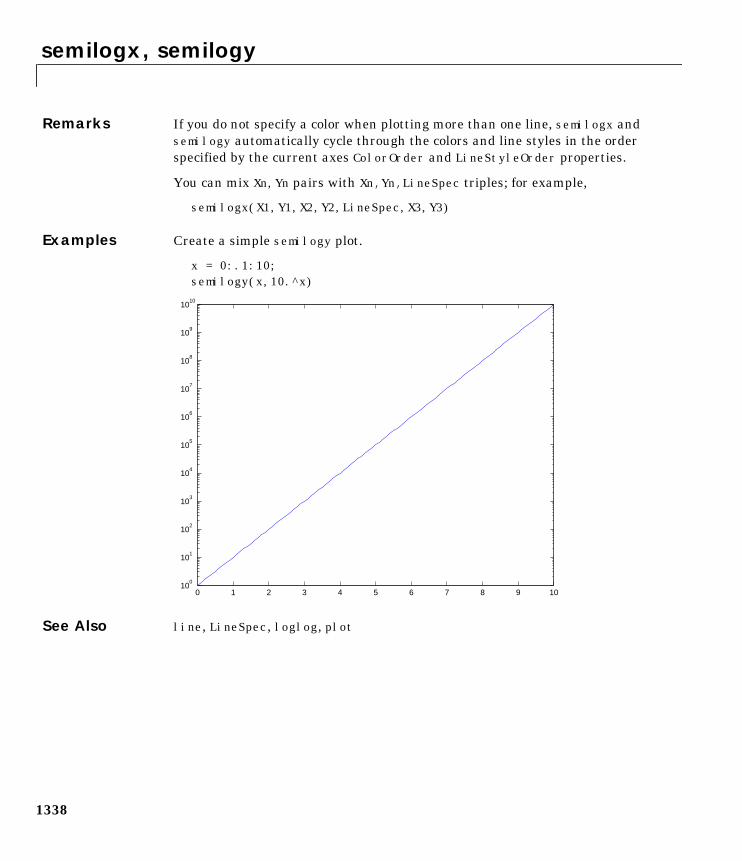
semilogx, semilogy
1338
Remarks If you do not specify a color when plotting more than one line, semilogx andsemilogy automatically cycle through the colors and line styles in the orderspecified by the current axes ColorOrder and LineStyleOrder properties.
You can mix Xn,Yn pairs with Xn, Yn, LineSpec triples; for example,
semilogx(X1,Y1,X2,Y2,LineSpec,X3,Y3)
Examples Create a simple semilogy plot.
x = 0:.1:10;semilogy(x,10.^x)
See Also line, LineSpec, loglog, plot
0 1 2 3 4 5 6 7 8 9 1010
0
101
102
103
104
105
106
107
108
109
1010
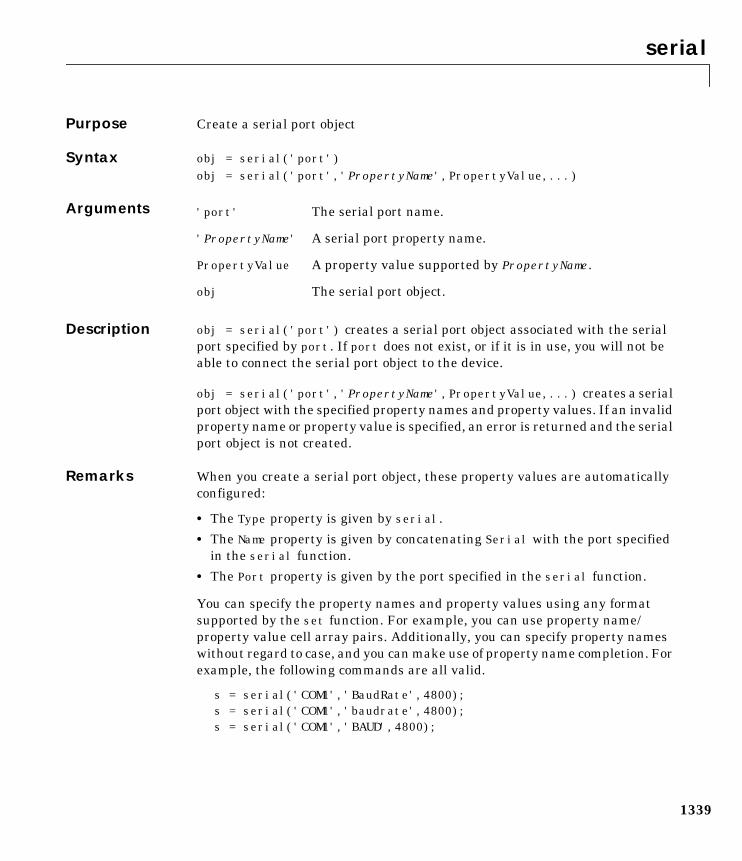
serial
1339
1serialPurpose Create a serial port object
Syntax obj = serial('port')obj = serial('port','PropertyName',PropertyValue,...)
Arguments
Description obj = serial('port') creates a serial port object associated with the serialport specified by port. If port does not exist, or if it is in use, you will not beable to connect the serial port object to the device.
obj = serial('port','PropertyName',PropertyValue,...) creates a serialport object with the specified property names and property values. If an invalidproperty name or property value is specified, an error is returned and the serialport object is not created.
Remarks When you create a serial port object, these property values are automaticallyconfigured:
• The Type property is given by serial.
• The Name property is given by concatenating Serial with the port specifiedin the serial function.
• The Port property is given by the port specified in the serial function.
You can specify the property names and property values using any formatsupported by the set function. For example, you can use property name/property value cell array pairs. Additionally, you can specify property nameswithout regard to case, and you can make use of property name completion. Forexample, the following commands are all valid.
s = serial('COM1','BaudRate',4800);s = serial('COM1','baudrate',4800);s = serial('COM1','BAUD',4800);
'port' The serial port name.
'PropertyName' A serial port property name.
PropertyValue A property value supported by PropertyName.
obj The serial port object.
serial
1340
Refer to “Configuring Property Values” on page 8-23 for a list of serial portobject properties that you can use with serial.
Before you can communicate with the device, it must be connected to obj withthe fopen function. A connected serial port object has a Status property valueof open. An error is returned if you attempt a read or write operation while theobject is not connected to the device. You can connect only one serial port objectto a given serial port.
Example This example creates the serial port object s1 associated with the serial portCOM1.
s1 = serial('COM1');
The Type, Name, and Port properties are automatically configured.
get(s1,'Type','Name','Port')ans = 'serial' 'Serial-COM1' 'COM1'
To specify properties during object creation
s2 = serial('COM2','BaudRate',1200,'DataBits',7);
See Also Functionsfclose, fopen
PropertiesName, Port, Status, Type
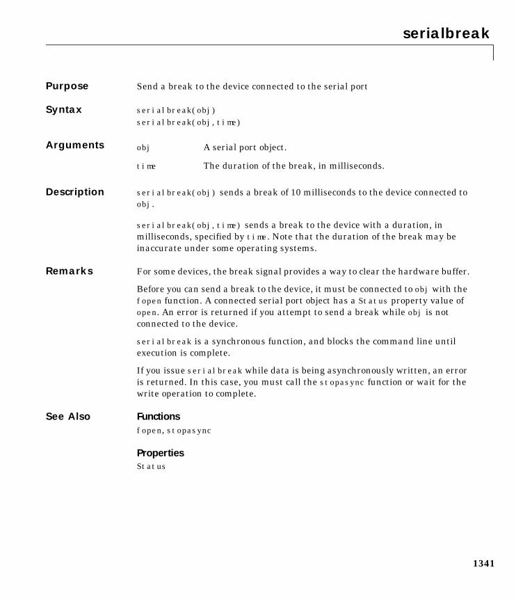
serialbreak
1341
1serialbreakPurpose Send a break to the device connected to the serial port
Syntax serialbreak(obj)serialbreak(obj,time)
Arguments
Description serialbreak(obj) sends a break of 10 milliseconds to the device connected toobj.
serialbreak(obj,time) sends a break to the device with a duration, inmilliseconds, specified by time. Note that the duration of the break may beinaccurate under some operating systems.
Remarks For some devices, the break signal provides a way to clear the hardware buffer.
Before you can send a break to the device, it must be connected to obj with thefopen function. A connected serial port object has a Status property value ofopen. An error is returned if you attempt to send a break while obj is notconnected to the device.
serialbreak is a synchronous function, and blocks the command line untilexecution is complete.
If you issue serialbreak while data is being asynchronously written, an erroris returned. In this case, you must call the stopasync function or wait for thewrite operation to complete.
See Also Functionsfopen, stopasync
PropertiesStatus
obj A serial port object.
time The duration of the break, in milliseconds.
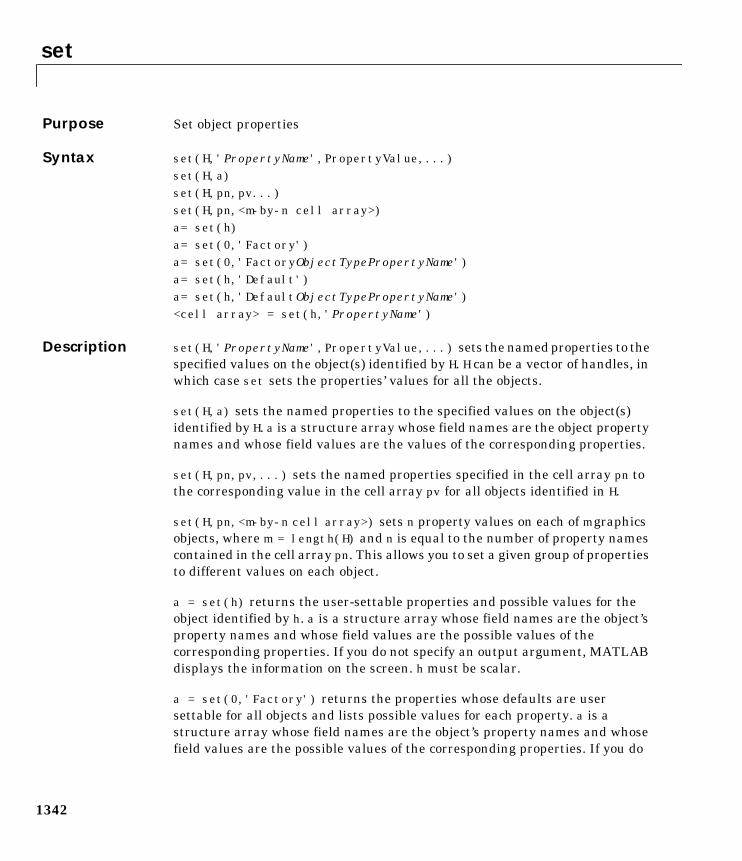
set
1342
1setPurpose Set object properties
Syntax set(H,'PropertyName',PropertyValue,...)set(H,a)set(H,pn,pv...)set(H,pn,<m-by-n cell array>)a= set(h)a= set(0,'Factory')a= set(0,'FactoryObjectTypePropertyName')a= set(h,'Default')a= set(h,'DefaultObjectTypePropertyName')<cell array> = set(h,'PropertyName')
Description set(H,'PropertyName',PropertyValue,...) sets the named properties to thespecified values on the object(s) identified by H. H can be a vector of handles, inwhich case set sets the properties’ values for all the objects.
set(H,a) sets the named properties to the specified values on the object(s)identified by H. a is a structure array whose field names are the object propertynames and whose field values are the values of the corresponding properties.
set(H,pn,pv,...) sets the named properties specified in the cell array pn tothe corresponding value in the cell array pv for all objects identified in H.
set(H,pn,<m-by-n cell array>) sets n property values on each of m graphicsobjects, where m = length(H) and n is equal to the number of property namescontained in the cell array pn. This allows you to set a given group of propertiesto different values on each object.
a = set(h) returns the user-settable properties and possible values for theobject identified by h. a is a structure array whose field names are the object’sproperty names and whose field values are the possible values of thecorresponding properties. If you do not specify an output argument, MATLABdisplays the information on the screen. h must be scalar.
a = set(0,'Factory') returns the properties whose defaults are usersettable for all objects and lists possible values for each property. a is astructure array whose field names are the object’s property names and whosefield values are the possible values of the corresponding properties. If you do
set
1343
not specify an output argument, MATLAB displays the information on thescreen.
a = set(0,'FactoryObjectTypePropertyName') returns the possible valuesof the named property for the specified object type, if the values are strings. Theargument FactoryObjectTypePropertyName is the word Factory concatenatedwith the object type (e.g., axes) and the property name (e.g., CameraPosition).
a = set(h,'Default') returns the names of properties having default valuesset on the object identified by h. set also returns the possible values if they arestrings. h must be scalar.
a = set(h,'DefaultObjectTypePropertyName') returns the possible valuesof the named property for the specified object type, if the values are strings. Theargument DefaultObjectTypePropertyName is the word Default concatenatedwith the object type (e.g., axes) and the property name (e.g., CameraPosition).For example, DefaultAxesCameraPosition. h must be scalar.
pv = set(h,'PropertyName') returns the possible values for the namedproperty. If the possible values are strings, set returns each in a cell of the cellarray, pv. For other properties, set returns an empty cell array. If you do notspecify an output argument, MATLAB displays the information on the screen.h must be scalar.
Remarks You can use any combination of property name/property value pairs, structurearrays, and cell arrays in one call to set.
Examples Set the Color property of the current axes to blue.
set(gca,'Color','b')
Change all the lines in a plot to black.
plot(peaks)set(findobj('Type','line'),'Color','k')
You can define a group of properties in a structure to better organize your code.For example, these statements define a structure called active, which containsa set of property definitions used for the uicontrol objects in a particular figure.
set
1344
When this figure becomes the current figure, MATLAB changes colors andenables the controls.
active.BackgroundColor = [.7 .7 .7];active.Enable = 'on';active.ForegroundColor = [0 0 0];
if gcf == control_fig_handleset(findobj(control_fig_handle,'Type','uicontrol'),active)
end
You can use cell arrays to set properties to different values on each object. Forexample, these statements define a cell array to set three properties,
PropName(1) = 'BackgroundColor';PropName(2) = 'Enable';PropName(3) = 'ForegroundColor';
These statements define a cell array containing three values for each of threeobjects (i.e., a 3-by-3 cell array).
PropVal(1,1) = [.5 .5 .5];PropVal(1,2) = 'off';PropVal(1,3) = [.9 .9 .9];
PropVal(2,1) = [1 0 0];PropVal(2,2) = 'on';PropVal(2,3) = [1 1 1];
PropVal(3,1) = [.7 .7 .7];PropVal(3,2) = 'on';PropVal(3,3) = [0 0 0];
Now pass the arguments to set,
set(H,PropName,PropVal)
where length(H) = 3 and each element is the handle to a uicontrol.
See Also findobj, gca, gcf, gco, gcbo, get
set (serial)
1345
1set (serial)Purpose Configure or display serial port object properties
Syntax set(obj)props = set(obj)set(obj,'PropertyName')props = set(obj,'PropertyName')set(obj,'PropertyName',PropertyValue,...)set(obj,PN,PV)set(obj,S)
Arguments
Description set(obj) displays all configurable properties values for obj. If a property hasa finite list of possible string values, then these values are also displayed.
props = set(obj) returns all configurable properties and their possiblevalues for obj to props. props is a structure whose field names are the propertynames of obj, and whose values are cell arrays of possible property values. Ifthe property does not have a finite set of possible values, then the cell array isempty.
set(obj,'PropertyName') displays the valid values for PropertyName if itpossesses a finite list of string values.
props = set(obj,'PropertyName') returns the valid values forPropertyName to props. props is a cell array of possible string values or anempty cell array if PropertyName does not have a finite list of possible values.
obj A serial port object or an array of serial port objects.
'PropertyName' A property name for obj.
PropertyValue A property value supported by PropertyName.
PN A cell array of property names.
PV A cell array of property values.
S A structure with property names and property values.
props A structure array whose field names are the propertynames for obj, or cell array of possible values.
set (serial)
1346
set(obj,'PropertyName',PropertyValue,...) configures multiple propertyvalues with a single command.
set(obj,PN,PV) configures the properties specified in the cell array of stringsPN to the corresponding values in the cell array PV. PN must be a vector. PV canbe m-by-n where m is equal to the number of serial port objects in obj and n isequal to the length of PN.
set(obj,S) configures the named properties to the specified values for obj. Sis a structure whose field names are serial port object properties, and whosefield values are the values of the corresponding properties.
Remarks Refer to “Configuring Property Values” on page 8-23 for a list of serial portobject properties that you can configure with set.
You can use any combination of property name/property value pairs,structures, and cell arrays in one call to set. Additionally, you can specify aproperty name without regard to case, and you can make use of property namecompletion. For example, if s is a serial port object, then the followingcommands are all valid.
set(s,'BaudRate')set(s,'baudrate')set(s,'BAUD')
If you use the help command to display help for set, then you need to supplythe pathname shown below.
help serial/set
Examples This example illustrates some of the ways you can use set to configure orreturn property values for the serial port object s.
s = serial('COM1');set(s,'BaudRate',9600,'Parity','even')set(s,'StopBits','RecordName',2,'sydney.txt')set(s,'Parity')[ none | odd | even | mark | space ]
See Also Functionsget
setappdata
1347
1setappdataPurpose Set application-defined data
Syntax setappdata(h,name,value)
Description setappdata(h,name,value) sets application-defined data for the object withhandle h. The application-defined data, which is created if it does not alreadyexist, is assigned a name and a value. value can be type of data.
See Also getappdata, isappdata, rmappdata
setdiff
1348
1setdiffPurpose Return the set difference of two vectors
Syntax c = setdiff(a,b)c = setdiff(A,B,'rows')[c,i] = setdiff(...)
Description c = setdiff(a,b) returns the values in a that are not in b. The resultingvector is sorted is ascending order. In set theoretic terms, c = a - b. a and bcan be cell arrays of strings.
c = setdiff(A,B,'rows') when A and B are matrices with the same numberof columns returns the rows from A that are not in B.
[c,i] = setdiff(...) also returns an index vector index such that c = a(i)or c = a(i,:).
Examples A = magic(5);B = magic(4);[c,i] = setdiff(A(:),B(:));c' = 17 18 19 20 21 22 23 24 25i' = 1 10 14 18 19 23 2 6 15
See Also intersect Set intersection of two vectorsismember True for a set membersetxor Set exclusive-or of two vectorsunion Set union of two vectorsunique Unique elements of a vector
setfield
1349
1setfieldPurpose Set field of structure array
Syntax s = setfield(s,'field',v)s = setfield(s,i,j,'field',k,v)
Description s = setfield(s,'field',v), where s is a 1-by-1 structure, sets the contentsof the specified field to the value v. This is equivalent to the syntaxs.field = v.
s = setfield(s,i,j,'field',k,v) sets the contents of the specifiedfield to the value v. This is equivalent to the syntax s(i,j).field(k) = v. Allsubscripts must be passed as cell arrays—that is, they must be enclosed incurly braces (similar toi,j and k above). Pass field references as strings.
Examples Given the structure:
mystr(1,1).name = 'alice';mystr(1,1).ID = 0;mystr(2,1).name = 'gertrude';mystr(2,1).ID = 1
Then the command mystr = setfield(mystr,2,1,'name','ted') yields
mystr =
2x1 struct array with fields: name ID
See Also getfield, rmfield, fieldnames
setstr
1350
1setstrPurpose Set string flag
Description This MATLAB 4 function has been renamed char in MATLAB 5.
See Also char Create character array (string)
setxor
1351
1setxorPurpose Set exclusive-or of two vectors
Syntax c = setxor(a,b)c = setxor(A,B,'rows')[c,ia,ib] = setxor(...)
Description c = setxor(a,b) returns the values that are not in the intersection of a and b.The resulting vector is sorted. a and b can be cell arrays of strings.
c = setxor(A,B,'rows') when A and B are matrices with the same numberof columns returns the rows that are not in the intersection of A and B.
[c,ia,ib] = setxor(...) also returns index vectors ia and ib such that c isa sorted combination of the elements c = a(ia) and c = b(ib) or, for rowcombinations, c = a(ia,:) and c = b(ib,:).
Examples a = [-1 0 1 Inf -Inf NaN];b = [-2 pi 0 Inf];c = setxor(a,b)
c = -Inf -2.0000 -1.0000 1.0000 3.1416 NaN
See Also intersect Set intersection of two vectorsismember True for a set membersetdiff Set difference of two vectorsunion Set union of two vectorsunique Unique elements of a vector
shading
1352
1shadingPurpose Set color shading properties
Syntax shading flatshading facetedshading interp
Description The shading function controls the color shading of surface and patch graphicsobjects.
shading flat each mesh line segment and face has a constant colordetermined by the color value at the end point of the segment or the corner ofthe face that has the smallest index or indices.
shading faceted flat shading with superimposed black mesh lines. This is thedefault shading mode.
shading interp varies the color in each line segment and face by interpolatingthe colormap index or true color value across the line or face.
Examples Compare a flat, faceted, and interpolated-shaded sphere.
subplot(3,1,1)sphere(16)axis squareshading flattitle('Flat Shading')
subplot(3,1,2)sphere(16)axis squareshading facetedtitle('Faceted Shading')
subplot(3,1,3)sphere(16)axis squareshading interptitle('Interpolated Shading')
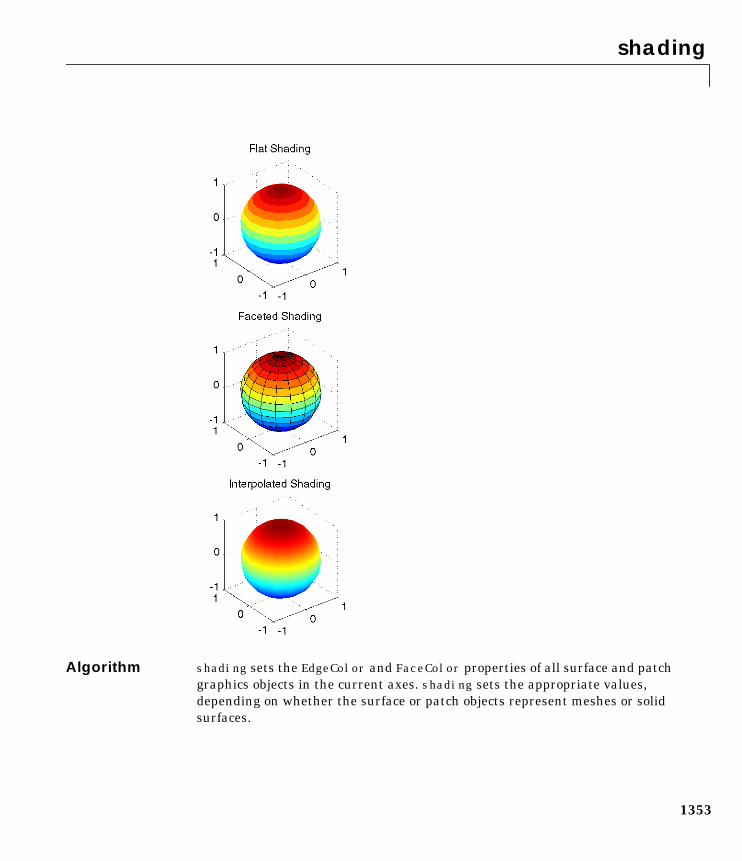
shading
1353
Algorithm shading sets the EdgeColor and FaceColor properties of all surface and patchgraphics objects in the current axes. shading sets the appropriate values,depending on whether the surface or patch objects represent meshes or solidsurfaces.
shading
1354
See Also fill, fill3, hidden, mesh, patch, pcolor, surfThe EdgeColor and FaceColor properties for surface and patch graphicsobjects.
shiftdim
1355
1shiftdimPurpose Shift dimensions
Syntax B = shiftdim(X,n)[B,nshifts] = shiftdim(X)
Description B = shiftdim(X,n) shifts the dimensions of X by n. When n is positive,shiftdim shifts the dimensions to the left and wraps the n leading dimensionsto the end. When n is negative, shiftdim shifts the dimensions to the right andpads with singletons.
[B,nshifts] = shiftdim(X) returns the array B with the same number ofelements as X but with any leading singleton dimensions removed. A singletondimension is any dimension for which size(A,dim) = 1. nshifts is the numberof dimensions that are removed.
If X is a scalar, shiftdim has no effect.
Examples The shiftdim command is handy for creating functions that, like sum or diff,work along the first nonsingleton dimension.
a = rand(1,1,3,1,2);[b,n] = shiftdim(a); % b is 3-by-1-by-2 and n is 2.c = shiftdim(b,-n); % c == a.d = shiftdim(a,3); % d is 1-by-2-by-1-by-1-by-3.
See Also reshape Reshape arraysqueeze Remove singleton dimensions
shrinkfaces
1356
1shrinkfacesPurpose Reduce the size of patch faces
Syntax shrinkfaces(p,sf)nfv = shrinkfaces(p,sf)nfv = shrinkfaces(fv,sf)shrinkfaces(p), shrinkfaces(fv)nfv = shrinkfaces(f,v,sf)[nf,nv] = shrinkfaces(...)
Description shrinkfaces(p,sf) shrinks the area of the faces in patch p to shrink factor sf.A shrink factor of 0.6 shrinks each face to 60% of its original area. If the patchcontains shared vertices, MATLAB creates nonshared vertices beforeperforming the face-area reduction.
nfv = shrinkfaces(p,sf) returns the face and vertex data in the struct nfv,but does not set the Faces and Vertices properties of patch p.
nfv = shrinkfaces(fv,sf) uses the face and vertex data from the struct fv.
shrinkfaces(p) and shrinkfaces(fv) (without specifying a shrink factor)assume a shrink factor of 0.3.
nfv = shrinkfaces(f,v,sf) uses the face and vertex data from the arrays fand v.
[nf,nv] = shrinkfaces(...) returns the face and vertex data in two separatearrays instead of a struct.
Examples This example uses the flow data set, which represents the speed profile of asubmerged jet within a infinite tank (type help flow for more information).Two isosurfaces provide a before and after view of the effects of shrinking theface size.
• First reducevolume samples the flow data at every other point and thenisosurface generates the faces and vertices data.
• The patch command accepts the face/vertex struct and draws the first (p1)isosurface.
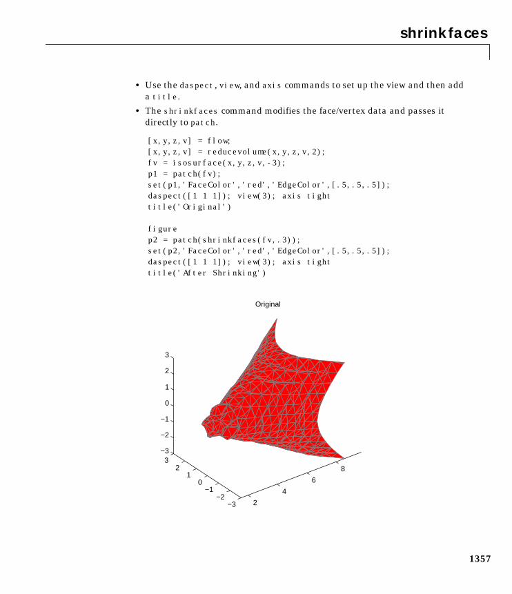
shrinkfaces
1357
• Use the daspect, view, and axis commands to set up the view and then adda title.
• The shrinkfaces command modifies the face/vertex data and passes itdirectly to patch.
[x,y,z,v] = flow;[x,y,z,v] = reducevolume(x,y,z,v,2);fv = isosurface(x,y,z,v,-3);p1 = patch(fv);set(p1,'FaceColor','red','EdgeColor',[.5,.5,.5]);daspect([1 1 1]); view(3); axis tighttitle('Original')
figurep2 = patch(shrinkfaces(fv,.3));set(p2,'FaceColor','red','EdgeColor',[.5,.5,.5]);daspect([1 1 1]); view(3); axis tighttitle('After Shrinking')
2
4
6
8
−3−2
−10
12
3−3
−2
−1
0
1
2
3
Original
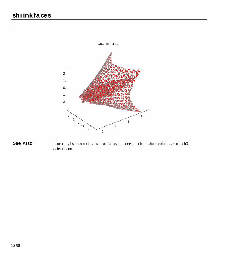
shrinkfaces
1358
See Also isocaps, isonormals, isosurface, reducepatch, reducevolume, smooth3,subvolume
2
4
6
8
−2−1
01
2
−2
−1
0
1
2
After Shrinking
sign
1359
1signPurpose Signum function
Syntax Y = sign(X)
Description Y = sign(X) returns an array Y the same size as X, where each element of Y is:
• 1 if the corresponding element of X is greater than zero
• 0 if the corresponding element of X equals zero
• -1 if the corresponding element of X is less than zero
For nonzero complex X, sign(X) = X./abs(X).
See Also abs Absolute value and complex magnitudeconj Complex conjugateimag Imaginary part of a complex numberreal Real part of complex number
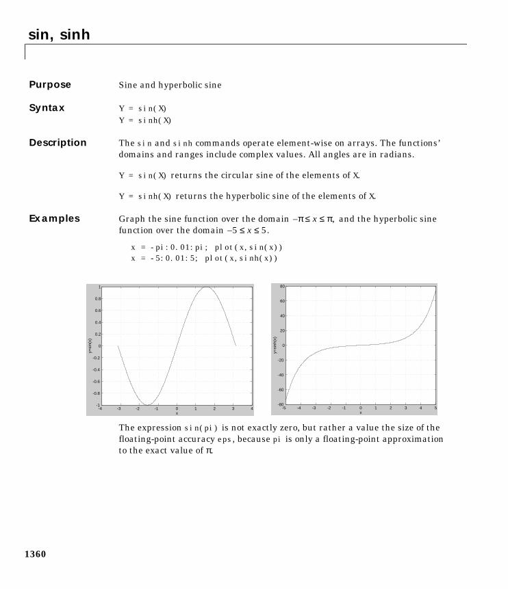
sin, sinh
1360
1sin, sinhPurpose Sine and hyperbolic sine
Syntax Y = sin(X)Y = sinh(X)
Description The sin and sinh commands operate element-wise on arrays. The functions’domains and ranges include complex values. All angles are in radians.
Y = sin(X) returns the circular sine of the elements of X.
Y = sinh(X) returns the hyperbolic sine of the elements of X.
Examples Graph the sine function over the domain and the hyperbolic sinefunction over the domain
x = -pi:0.01:pi; plot(x,sin(x))x = -5:0.01:5; plot(x,sinh(x))
The expression sin(pi) is not exactly zero, but rather a value the size of thefloating-point accuracy eps, because pi is only a floating-point approximationto the exact value of π.
π– x π,≤ ≤5– x 5.≤ ≤
-4 -3 -2 -1 0 1 2 3 4-1
-0.8
-0.6
-0.4
-0.2
0
0.2
0.4
0.6
0.8
1
x
y=si
n(x)
-5 -4 -3 -2 -1 0 1 2 3 4 5-80
-60
-40
-20
0
20
40
60
80
x
y=si
nh(x
)
sin, sinh
1361
Algorithm
See Also asin, asinh Inverse sine and inverse hyperbolic sine
x iy+( )sin x( ) y( )cossin i x( ) y( )sincos+=
z( )sin eiz e iz––2i
----------------------=
z( )sinh ez e z––2
-------------------=
single
1362
1singlePurpose Convert to single-precision
Syntax B = single(A)
Description B = single(A) converts the matrix A to single-precision, returning that valuein B. A can be any numeric object (such as a double). If A is alreadysingle-precision, single has no effect. Single-precision quantities require lessstorage than double-precision quantities, but have less precision and a smallerrange.
The single class is primarily meant to be used to store single-precision values.Hence most operations that manipulate arrays without changing theirelements are defined. Examples are reshape, size, the relational operators,subscripted assignment and subscripted reference. No math operations aredefined for single objects.
You can define your own methods for the single class by placing theappropriately named method in an @single directory within a directory onyour path.
Examples a = magic(4);b = single(a);
whos Name Size Bytes Class
a 4x4 128 double array b 4x4 64 single array
See Also double
size
1363
1sizePurpose Array dimensions
Syntax d = size(X)[m,n] = size(X)m = size(X,dim)[d1,d2,d3,...,dn] = size(X)
Description d = size(X) returns the sizes of each dimension of array X in a vector d withndims(X) elements.
[m,n] = size(X) returns the size of matrix X in variables m and n.
m = size(X,dim) returns the size of the dimension of X specified by scalar dim.
[d1,d2,d3,...,dn] = size(X) returns the sizes of the various dimensions ofarray X in separate variables.
If the number of output arguments n does not equal ndims(X), then:
Examples The size of the second dimension of rand(2,3,4) is 3.
m = size(rand(2,3,4),2)
m = 3
Here the size is output as a single vector.
d = size(rand(2,3,4))
d = 2 3 4
Here the size of each dimension is assigned to a separate variable.
If n > ndims(X) Ones are returned in the “extra” variables dndims(X)+1through dn.
If n < ndims(X) The final variable dn contains the product of the sizes ofall the “remaining” dimensions of X, that is, dimensionsn+1 through ndims(X).
size
1364
[m,n,p] = size(rand(2,3,4))m = 2
n = 3
p = 4
If X = ones(3,4,5), then
[d1,d2,d3] = size(X)
d1 = d2 = d3 =3 4 5
but when the number of output variables is less than ndims(X):
[d1,d2] = size(X)
d1 = d2 =3 20
The “extra” dimensions are collapsed into a single product.
If n > ndims(X), the “extra” variables all represent singleton dimensions:
[d1,d2,d3,d4,d5,d6] = size(X)
d1 = d2 = d3 =3 4 5
d4 = d5 = d6 = 1 1 1
See Also exist Check if a variable or file existslength Length of vectorwhos List directory of variables in memory
size (serial)
1365
1size (serial)Purpose Size of serial port object array
Syntax d = size(obj)[m,n] = size(obj)[m1,m2,...,mn] = size(obj)m = size(obj,dim)
Arguments
Description d = size(obj) returns the two-element row vector d containing the number ofrows and columns in obj.
[m,n] = size(obj) returns the number of rows and columns in separateoutput variables.
[m1,m2,m3,...,mn] = size(obj) returns the length of the first n dimensionsof obj.
m = size(obj,dim) returns the length of the dimension specified by the scalardim. For example, size(obj,1) returns the number of rows.
See Also Functionslength
obj A serial port object or an array of serial port objects.
dim The dimension of obj.
d The number of rows and columns in obj.
m The number of rows in obj, or the length of the dimensionspecified by dim.
n The number of columns in obj.
m1,m2,...,mn The length of the first N dimensions of obj.
slice
1366
1slicePurpose Volumetric slice plot
Syntax slice(V,sx,sy,sz)slice(X,Y,Z,V,sx,sy,sz)slice(V,XI,YI,ZI)slice(X,Y,Z,V,XI,YI,ZI)slice(...,'method')h = slice(...)
Description slice displays orthogonal slice planes through volumetric data.
slice(V,sx,sy,sz) draws slices along the x, y, z directions in the volume V atthe points in the vectors sx, sy, and sz. V is an m-by-n-by-p volume arraycontaining data values at the default location X = 1:n, Y = 1:m, Z = 1:p. Eachelement in the vectors sx, sy, and sz defines a slice plane in the x-, y-, or z-axisdirection.
slice(X,Y,Z,V,sx,sy,sz) draws slices of the volume V. X, Y, and Z arethree-dimensional arrays specifying the coordinates for V. X, Y, and Z must bemonotonic and orthogonally spaced (as if produced by the function meshgrid).The color at each point is determined by 3-D interpolation into the volume V.
slice(V,XI,YI,ZI) draws data in the volume V for the slices defined by XI, YI,and ZI. XI, YI, and ZI are matrices that define a surface, and the volume isevaluated at the surface points. XI, YI, and ZI must all be the same size.
slice(X,Y,Z,V,XI,YI,ZI) draws slices through the volume V along thesurface defined by the arrays XI, YI, ZI.
slice(...,'method') specifies the interpolation method. 'method' is'linear', 'cubic', or 'nearest'.
• linear specifies trilinear interpolation (the default).
• cubic specifies tricubic interpolation.
• nearest specifies nearest neighbor interpolation.
h = slice(...) returns a vector of handles to surface graphics objects.
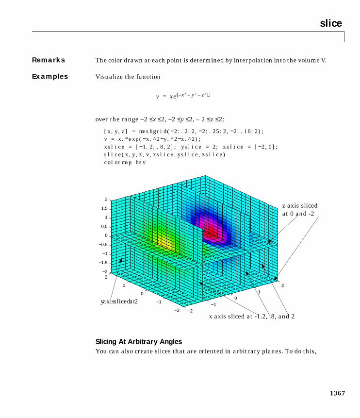
slice
1367
Remarks The color drawn at each point is determined by interpolation into the volume V.
Examples Visualize the function
over the range –2 ≤x ≤2, –2 ≤y ≤2, – 2 ≤z ≤2:
[x,y,z] = meshgrid(−2:.2:2,−2:.25:2,−2:.16:2);v = x.*exp(−x.^2−y.^2−z.^2);xslice = [−1.2,.8,2]; yslice = 2; zslice = [−2,0];slice(x,y,z,v,xslice,yslice,zslice)colormap hsv
Slicing At Arbitrary AnglesYou can also create slices that are oriented in arbitrary planes. To do this,
v xe x2 y2– z2––( )=
−2−1
01
2
−2
−1
0
1
2−2
−1.5
−1
−0.5
0
0.5
1
1.5
2
x axis sliced at -1.2, .8, and 2
yaxisslicedat2
z axis slicedat 0 and -2
slice
1368
• Create a slice surface in the domain of the volume (surf, linspace).
• Orient this surface with respect the the axes (rotate).
• Get the XData, YData, and ZData of the surface (get).
• Use this data to draw the slice plane within the volume.
For example, these statements slice the volume in the first example with arotated plane. Placing these commands within a for loop “passes” the planethrough the volume along the z-axis.
for i = −2:.5:2hsp = surf(linspace(−2,2,20),linspace(−2,2,20),zeros(20)+i);rotate(hsp,[1,−1,1],30)xd = get(hsp,’XData’);yd = get(hsp,’YData’);zd = get(hsp,’ZData’);delete(hsp)slice(x,y,z,v,[−2,2],2,-2) % Draw some volume boundarieshold onslice(x,y,z,v,xd,yd,zd)hold offaxis tightview(−5,10)drawnow
end
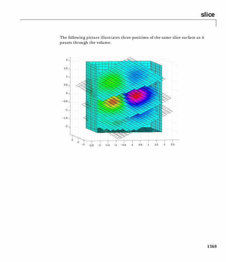
slice
1369
The following picture illustrates three positions of the same slice surface as itpasses through the volume.
−2.5 −2 −1.5 −1 −0.5 0 0.5 1 1.5 2 2.5−20
2
−2
−1.5
−1
−0.5
0
0.5
1
1.5
2
slice
1370
Slicing with a Nonplanar SurfaceYou can slice the volume with any surface. This example probes the volumecreated in the previous example by passing a spherical slice surface throughthe volume.
[xsp,ysp,zsp] = sphere;slice(x,y,z,v,[-2,2],2,-2) % Draw some volume boundaries
for i = -3:.2:3hsp = surface(xsp+i,ysp,zsp);rotate(hsp,[1 0 0],90)xd = get(hsp,’XData’);yd = get(hsp,’YData’);zd = get(hsp,’ZData’);delete(hsp)hold onhslicer = slice(x,y,z,v,xd,yd,zd);axis tightxlim([-3,3])view(-10,35)drawnowdelete(hslicer)hold off
end
The following picture illustrates three positions of the spherical slice surface asit passes through the volume.
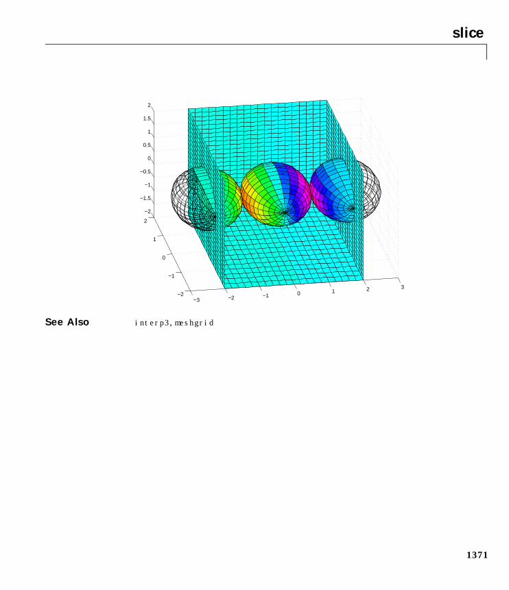
slice
1371
See Also interp3, meshgrid
−3 −2 −1 0 1 2 3−2
−1
0
1
2
−2
−1.5
−1
−0.5
0
0.5
1
1.5
2
smooth3
1372
1smooth3Purpose Smooth 3-D data
Syntax W = smooth3(V)W = smooth3(V,'filter')W = smooth3(V,'filter',size)W = smooth3(V,'filter',size,sd)
Description W = smooth3(V) smooths the input data V and returns the smoothed data in W.
W = smooth3(V,'filter') filter determines the convolution kernel and canbe the strings gaussian or box (default).
W = smooth3(V,'filter',size) sets the size of the convolution kernel (defaultis [3 3 3]). If size is scalar, then size is interpreted as [size, size, size].
W = smooth3(V,'filter',size,sd) sets an attribute of the convolution kernel.When filter is gaussian, sd is the standard deviation (default is .65).
Examples This example smooths some random 3-D data and then creates an isosurfacewith end caps.
data = rand(10,10,10);data = smooth3(data,'box',5);p1 = patch(isosurface(data,.5), ... 'FaceColor','blue','EdgeColor','none');p2 = patch(isocaps(data,.5), ... 'FaceColor','interp','EdgeColor','none');isonormals(data,p1)view(3); axis vis3d tightcamlight; lighting phong
See Also isocaps, isonormals, isosurface, patch, reducepatch, reducevolume,subvolume
sort
1373
1sortPurpose Sort elements in ascending order
Syntax B = sort(A)B = sort(A,dim)[B,INDEX] = sort(A,...)
Description B = sort(A) sorts the elements along different dimensions of an array, andarranges those elements in ascending order. A can be a cell array of strings.
Real, complex, and string elements are permitted. For identical values in A, thelocation in the input array determines location in the sorted list. When A iscomplex, the elements are sorted by magnitude, and where magnitudes areequal, further sorted by phase angle on the interval . If A includes anyNaN elements, sort places these at the end.
If A is a vector, sort(A) arranges those elements in ascending order.
If A is a matrix, sort(A) treats the columns of A as vectors, returning sortedcolumns.
If A is a multidimensional array, sort(A) treats the values along the firstnon-singleton dimension as vectors, returning an array of sorted vectors.
B = sort(A,dim) sorts the elements along the dimension of A specified by ascalar dim.
If dim is a vector, sort works iteratively on the specified dimensions. Thus,sort(A,[1 2]) is equivalent to sort(sort(A,2),1).
[B,INDEX] = sort(A,...) also returns an array of indices. INDEX is an arrayof size(A), each column of which is a permutation vector of the correspondingcolumn of A. If A has repeated elements of equal value, indices are returned thatpreserve the original relative ordering.
See Also max, mean, median, min, sortrows
π π,–[ ]
sortrows
1374
1sortrowsPurpose Sort rows in ascending order
Syntax B = sortrows(A)B = sortrows(A,column)[B,index] = sortrows(A)
Description B = sortrows(A) sorts the rows of A as a group in ascending order. ArgumentA must be either a matrix or a column vector.
For strings, this is the familiar dictionary sort. When A is complex, theelements are sorted by magnitude, and, where magnitudes are equal, furthersorted by phase angle on the interval .
B = sortrows(A,column) sorts the matrix based on the columns specified inthe vector column. For example, sortrows(A,[2 3]) sorts the rows of A by thesecond column, and where these are equal, further sorts by the third column.
[B,index] = sortrows(A) also returns an index vector index.
If A is a column vector, then B = A(index).
If A is an m-by-n matrix, then B = A(index,:).
Examples Given the 5-by-5 string matrix,
A = ['one ';'two ';'three';'four ';'five '];
The commands B = sortrows(A) and C = sortrows(A,1) yield
B = C =five fourfour fiveone onethree twotwo three
See Also sort Sort elements in ascending order
π π,–[ ]
sound
1375
1soundPurpose Convert vector into sound
Syntax sound(y,Fs)sound(y)sound(y,Fs,bits)
Description sound(y,Fs), sends the signal in vector y (with sample frequency Fs) to thespeaker on PC, Macintosh, and most UNIX platforms. Values in y are assumedto be in the range . Values outside that range are clipped. Stereosound is played on platforms that support it when y is an n-by-2 matrix.
sound(y) plays the sound at the default sample rate or 8192 Hz.
sound(y,Fs,bits) plays the sound using bits bits/sample if possible. Mostplatforms support bits = 8 or bits = 16.
Remarks MATLAB supports all Windows-compatible sound devices.
See Also auread Read NeXT/SUN (.au) sound fileauwrite Write NeXT/SUN (.au) sound filesoundsc Scale data and play as soundwavread Read Microsoft WAVE (.wav) sound filewavwrite Write Microsoft WAVE (.wav) sound file
1.0 y 1.0≤ ≤–
soundcap
1376
1soundcapPurpose Sound capabilities
Syntax soundcap
Description soundcap prints the computer’s sound capabilities, including whether or notthe computer can play stereo sound and record sound, the sampling ratessupported for recording, and the resolution supported for recording andplayback.
soundsc
1377
1soundscPurpose Scale data and play as sound
Syntax soundsc(y,Fs)soundsc(y)soundsc(y,Fs,bits)soundsc(y,...,slim)
Description soundsc(y,Fs) sends the signal in vector y (with sample frequency Fs) to thespeaker on PC, Macintosh, and most UNIX platforms. The signal y is scaled tothe range before it is played, resulting in a sound that is playedas loud as possible without clipping.
soundsc(y) plays the sound at the default sample rate or 8192 Hz.
soundsc(y,Fs,bits) plays the sound using bits bits/sample if possible. Mostplatforms support bits = 8 or bits = 16.
soundsc(y,...,slim) where slim = [slow shigh] maps the values in ybetween slow and shigh to the full sound range. The default value isslim = [min(y) max(y)].
Remarks MATLAB supports all Windows-compatible sound devices.
See Also auread Read NeXT/SUN (.au) sound fileauwrite Write NeXT/SUN (.au) sound filesound Convert vector into soundwavread Read Microsoft WAVE (.wav) sound filewavwrite Write Microsoft WAVE (.wav) sound file
1.0 y 1.0≤ ≤–
spalloc
1378
1spallocPurpose Allocate space for sparse matrix
Syntax S = spalloc(m,n,nzmax)
Description S = spalloc(m,n,nzmax) creates an all zero sparse matrix S of size m-by-nwith room to hold nzmax nonzeros. The matrix can then be generated columnby column without requiring repeated storage allocation as the number ofnonzeros grows.
spalloc(m,n,nzmax) is shorthand for
sparse([],[],[],m,n,nzmax)
Examples To generate efficiently a sparse matrix that has an average of at most threenonzero elements per column
S = spalloc(n,n,3∗n);for j = 1:n
S(:,j) = [zeros(n-3,1)' round(rand(3,1))']';end
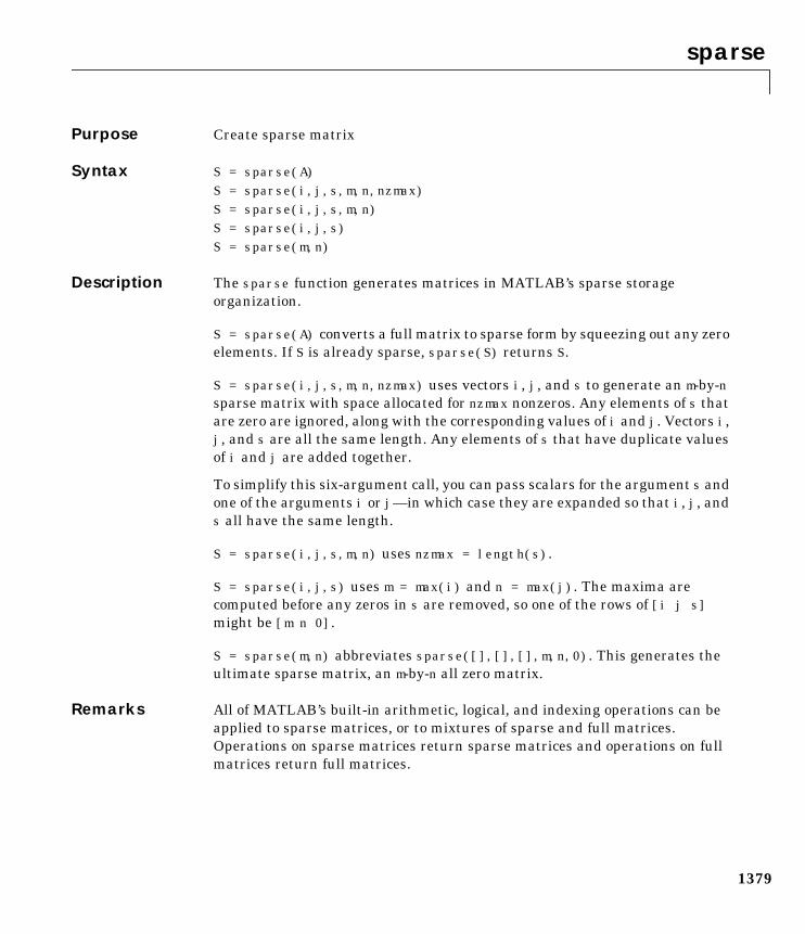
sparse
1379
1sparsePurpose Create sparse matrix
Syntax S = sparse(A)S = sparse(i,j,s,m,n,nzmax)S = sparse(i,j,s,m,n)S = sparse(i,j,s)S = sparse(m,n)
Description The sparse function generates matrices in MATLAB’s sparse storageorganization.
S = sparse(A) converts a full matrix to sparse form by squeezing out any zeroelements. If S is already sparse, sparse(S) returns S.
S = sparse(i,j,s,m,n,nzmax) uses vectors i, j, and s to generate an m-by-nsparse matrix with space allocated for nzmax nonzeros. Any elements of s thatare zero are ignored, along with the corresponding values of i and j. Vectors i,j, and s are all the same length. Any elements of s that have duplicate valuesof i and j are added together.
To simplify this six-argument call, you can pass scalars for the argument s andone of the arguments i or j—in which case they are expanded so that i, j, ands all have the same length.
S = sparse(i,j,s,m,n) uses nzmax = length(s).
S = sparse(i,j,s) uses m = max(i) and n = max(j). The maxima arecomputed before any zeros in s are removed, so one of the rows of [i j s]might be [m n 0].
S = sparse(m,n) abbreviates sparse([],[],[],m,n,0). This generates theultimate sparse matrix, an m-by-n all zero matrix.
Remarks All of MATLAB’s built-in arithmetic, logical, and indexing operations can beapplied to sparse matrices, or to mixtures of sparse and full matrices.Operations on sparse matrices return sparse matrices and operations on fullmatrices return full matrices.
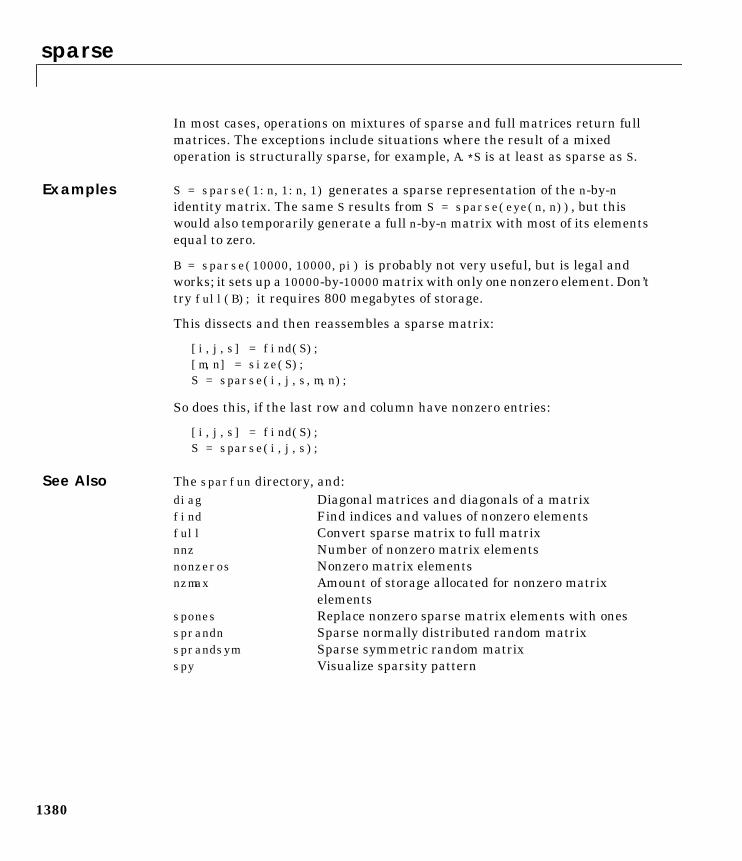
sparse
1380
In most cases, operations on mixtures of sparse and full matrices return fullmatrices. The exceptions include situations where the result of a mixedoperation is structurally sparse, for example, A.∗S is at least as sparse as S.
Examples S = sparse(1:n,1:n,1) generates a sparse representation of the n-by-nidentity matrix. The same S results from S = sparse(eye(n,n)), but thiswould also temporarily generate a full n-by-n matrix with most of its elementsequal to zero.
B = sparse(10000,10000,pi) is probably not very useful, but is legal andworks; it sets up a 10000-by-10000matrix with only one nonzero element. Don’ttry full(B); it requires 800 megabytes of storage.
This dissects and then reassembles a sparse matrix:
[i,j,s] = find(S);[m,n] = size(S);S = sparse(i,j,s,m,n);
So does this, if the last row and column have nonzero entries:
[i,j,s] = find(S);S = sparse(i,j,s);
See Also The sparfun directory, and:diag Diagonal matrices and diagonals of a matrixfind Find indices and values of nonzero elementsfull Convert sparse matrix to full matrixnnz Number of nonzero matrix elementsnonzeros Nonzero matrix elementsnzmax Amount of storage allocated for nonzero matrix
elementsspones Replace nonzero sparse matrix elements with onessprandn Sparse normally distributed random matrixsprandsym Sparse symmetric random matrixspy Visualize sparsity pattern
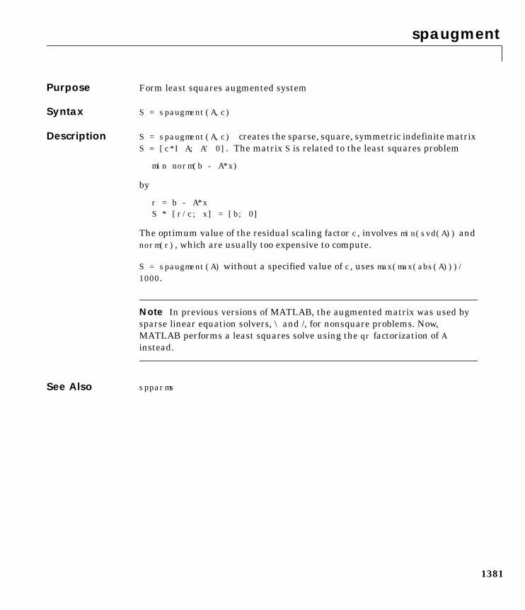
spaugment
1381
1spaugmentPurpose Form least squares augmented system
Syntax S = spaugment(A,c)
Description S = spaugment(A,c) creates the sparse, square, symmetric indefinite matrixS = [c*I A; A' 0]. The matrix S is related to the least squares problem
min norm(b - A*x)
by
r = b - A*xS * [r/c; x] = [b; 0]
The optimum value of the residual scaling factor c, involves min(svd(A)) andnorm(r), which are usually too expensive to compute.
S = spaugment(A) without a specified value of c, uses max(max(abs(A)))/1000.
Note In previous versions of MATLAB, the augmented matrix was used bysparse linear equation solvers, \ and /, for nonsquare problems. Now,MATLAB performs a least squares solve using the qr factorization of Ainstead.
See Also spparms
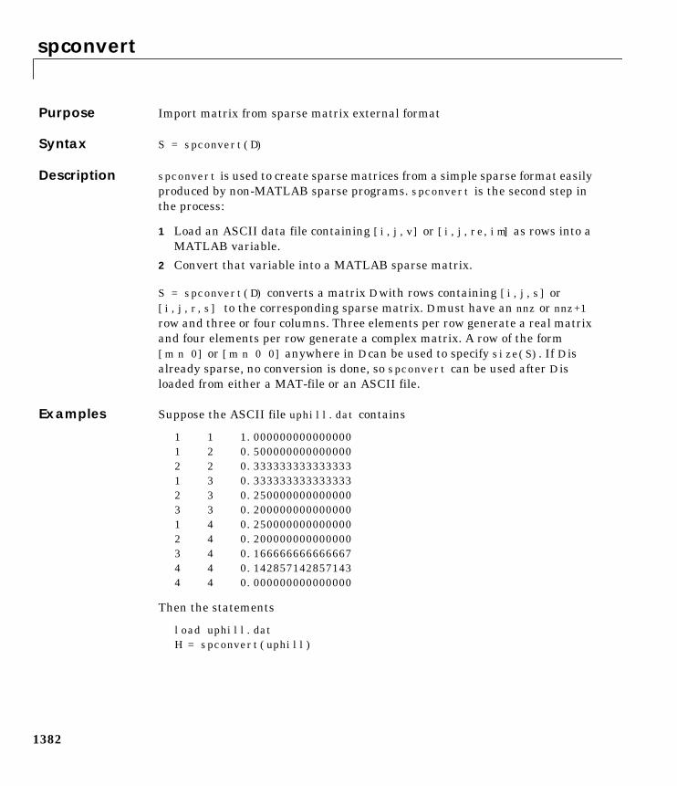
spconvert
1382
1spconvertPurpose Import matrix from sparse matrix external format
Syntax S = spconvert(D)
Description spconvert is used to create sparse matrices from a simple sparse format easilyproduced by non-MATLAB sparse programs. spconvert is the second step inthe process:
1 Load an ASCII data file containing [i,j,v] or [i,j,re,im] as rows into aMATLAB variable.
2 Convert that variable into a MATLAB sparse matrix.
S = spconvert(D) converts a matrix D with rows containing [i,j,s] or[i,j,r,s] to the corresponding sparse matrix. D must have an nnz or nnz+1row and three or four columns. Three elements per row generate a real matrixand four elements per row generate a complex matrix. A row of the form[m n 0] or [m n 0 0] anywhere in D can be used to specify size(S). If D isalready sparse, no conversion is done, so spconvert can be used after D isloaded from either a MAT-file or an ASCII file.
Examples Suppose the ASCII file uphill.dat contains
1 1 1.0000000000000001 2 0.5000000000000002 2 0.3333333333333331 3 0.3333333333333332 3 0.2500000000000003 3 0.2000000000000001 4 0.2500000000000002 4 0.2000000000000003 4 0.1666666666666674 4 0.1428571428571434 4 0.000000000000000
Then the statements
load uphill.datH = spconvert(uphill)
spconvert
1383
recreate sparse(triu(hilb(4))), possibly with roundoff errors. In this case,the last line of the input file is not necessary because the earlier lines alreadyspecify that the matrix is at least 4-by-4.
spdiags
1384
1spdiagsPurpose Extract and create sparse band and diagonal matrices
Syntax [B,d] = spdiags(A)B = spdiags(A,d)A = spdiags(B,d,A)A = spdiags(B,d,m,n)
Description The spdiags function generalizes the function diag. Four different operations,distinguished by the number of input arguments, are possible:
[B,d] = spdiags(A) extracts all nonzero diagonals from the m-by-n matrix A.B is a min(m,n)-by-p matrix whose columns are the p nonzero diagonals of A. dis a vector of length p whose integer components specify the diagonals in A.
B = spdiags(A,d) extracts the diagonals specified by d.
A = spdiags(B,d,A) replaces the diagonals specified by d with the columns ofB. The output is sparse.
A = spdiags(B,d,m,n) creates an m-by-n sparse matrix by taking the columnsof B and placing them along the diagonals specified by d.
Note If a column of B is longer than the diagonal it’s replacing, spdiags takeselements of super-diagonals from the lower part of the column of B, andelements of sub-diagonals from the upper part of the column of B.
Arguments The spdiags function deals with three matrices, in various combinations, asboth input and output:
A An m-by-n matrix, usually (but not necessarily) sparse, with its nonzeroor specified elements located on p diagonals.
B A min(m,n)-by-p matrix, usually (but not necessarily) full, whosecolumns are the diagonals of A.
d A vector of length p whose integer components specify the diagonals inA.
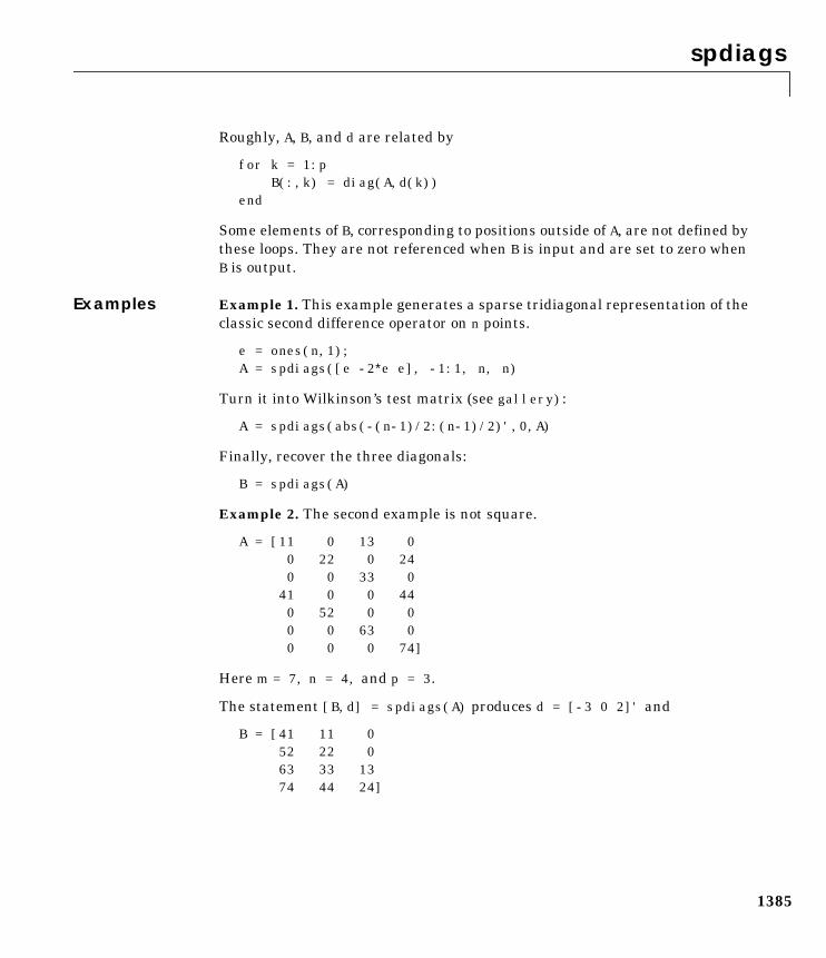
spdiags
1385
Roughly, A, B, and d are related by
for k = 1:pB(:,k) = diag(A,d(k))
end
Some elements of B, corresponding to positions outside of A, are not defined bythese loops. They are not referenced when B is input and are set to zero whenB is output.
Examples Example 1. This example generates a sparse tridiagonal representation of theclassic second difference operator on n points.
e = ones(n,1);A = spdiags([e -2∗e e], -1:1, n, n)
Turn it into Wilkinson’s test matrix (see gallery):
A = spdiags(abs(-(n-1)/2:(n-1)/2)',0,A)
Finally, recover the three diagonals:
B = spdiags(A)
Example 2. The second example is not square.
A = [11 0 13 00 22 0 240 0 33 0
41 0 0 440 52 0 00 0 63 00 0 0 74]
Here m = 7, n = 4, and p = 3.
The statement [B,d] = spdiags(A) produces d = [-3 0 2]' and
B = [41 11 052 22 063 33 1374 44 24]
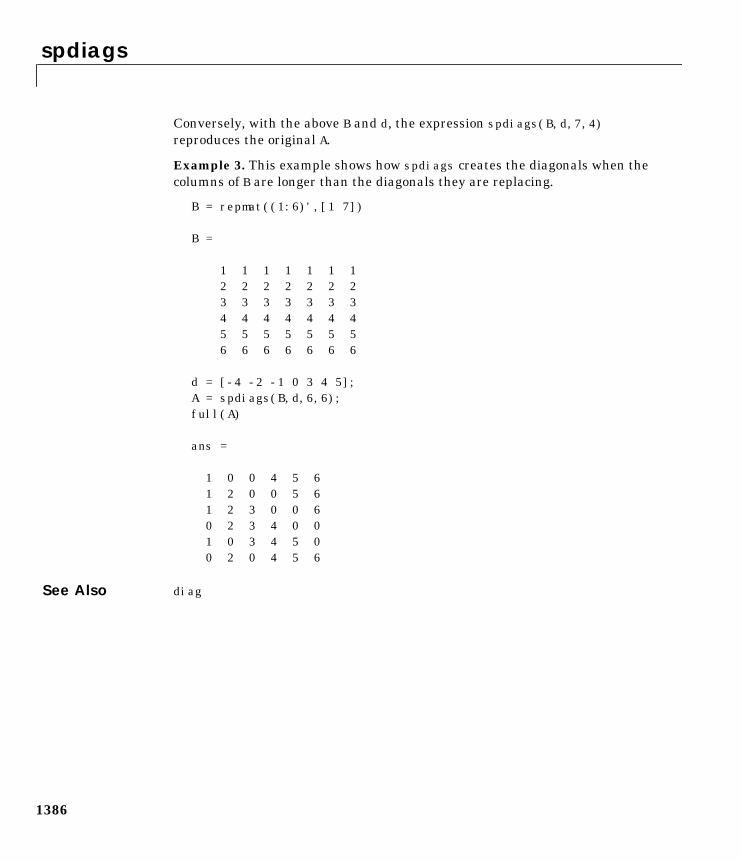
spdiags
1386
Conversely, with the above B and d, the expression spdiags(B,d,7,4)reproduces the original A.
Example 3. This example shows how spdiags creates the diagonals when thecolumns of B are longer than the diagonals they are replacing.
B = repmat((1:6)',[1 7])
B =
1 1 1 1 1 1 1 2 2 2 2 2 2 2 3 3 3 3 3 3 3 4 4 4 4 4 4 4 5 5 5 5 5 5 5 6 6 6 6 6 6 6
d = [-4 -2 -1 0 3 4 5];A = spdiags(B,d,6,6);full(A)
ans =
1 0 0 4 5 6 1 2 0 0 5 6 1 2 3 0 0 6 0 2 3 4 0 0 1 0 3 4 5 0 0 2 0 4 5 6
See Also diag
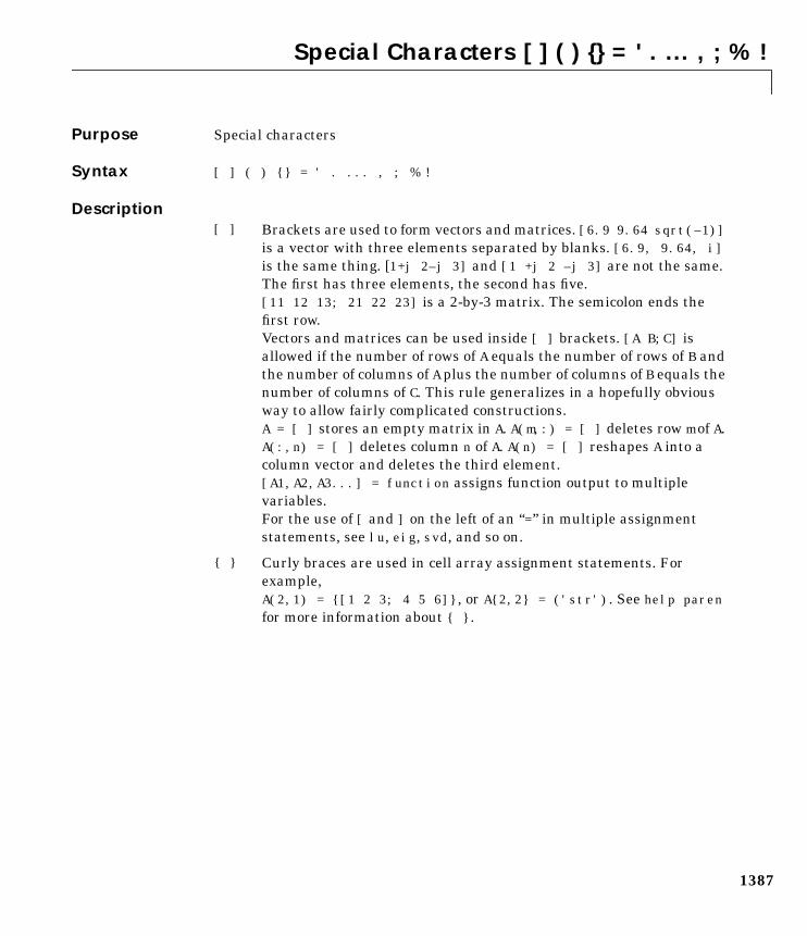
Special Characters [ ] ( ) = ' . ... , ; % !
1387
1Special Characters [ ] ( ) = ' . ... , ; % !Purpose Special characters
Syntax [ ] ( ) = ' . ... , ; % !
Description[ ] Brackets are used to form vectors and matrices. [6.9 9.64 sqrt(–1)]
is a vector with three elements separated by blanks. [6.9, 9.64, i]is the same thing. [1+j 2–j 3] and [1 +j 2 –j 3] are not the same.The first has three elements, the second has five.[11 12 13; 21 22 23] is a 2-by-3 matrix. The semicolon ends thefirst row.Vectors and matrices can be used inside [ ] brackets. [A B;C] isallowed if the number of rows of A equals the number of rows of B andthe number of columns of A plus the number of columns of B equals thenumber of columns of C. This rule generalizes in a hopefully obviousway to allow fairly complicated constructions.A = [ ] stores an empty matrix in A. A(m,:) = [ ] deletes row m of A.A(:,n) = [ ] deletes column n of A. A(n) = [ ] reshapes A into acolumn vector and deletes the third element.[A1,A2,A3...] = function assigns function output to multiplevariables.For the use of [ and ] on the left of an “=” in multiple assignmentstatements, see lu, eig, svd, and so on.
Curly braces are used in cell array assignment statements. Forexample,A(2,1) = [1 2 3; 4 5 6], or A2,2 = ('str'). See help parenfor more information about .
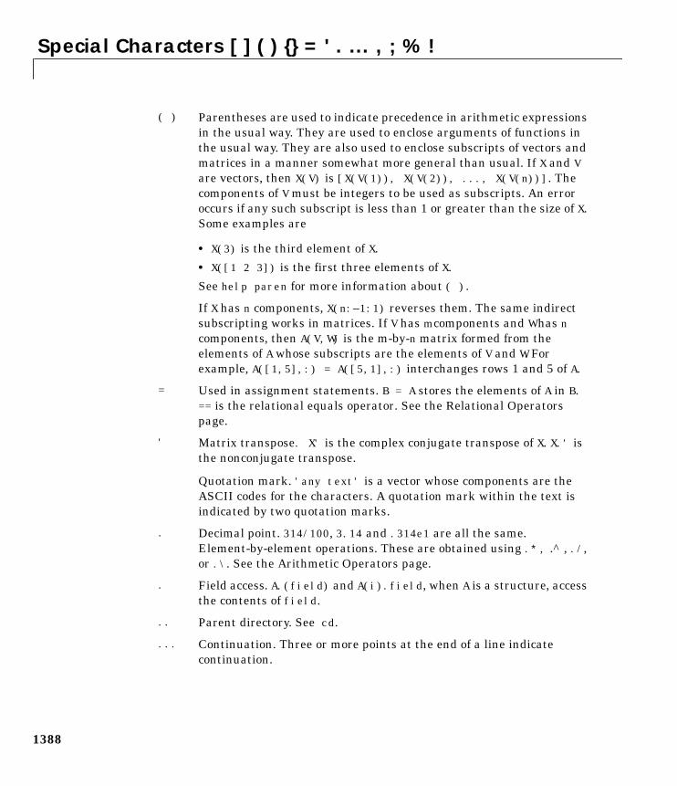
Special Characters [ ] ( ) = ' . ... , ; % !
1388
( ) Parentheses are used to indicate precedence in arithmetic expressionsin the usual way. They are used to enclose arguments of functions inthe usual way. They are also used to enclose subscripts of vectors andmatrices in a manner somewhat more general than usual. If X and Vare vectors, then X(V) is [X(V(1)), X(V(2)), ..., X(V(n))]. Thecomponents of V must be integers to be used as subscripts. An erroroccurs if any such subscript is less than 1 or greater than the size of X.Some examples are
• X(3) is the third element of X.
• X([1 2 3]) is the first three elements of X.
See help paren for more information about ( ).
If X has n components, X(n:–1:1) reverses them. The same indirectsubscripting works in matrices. If V has m components and W has ncomponents, then A(V,W) is the m-by-n matrix formed from theelements of A whose subscripts are the elements of V and W. Forexample, A([1,5],:) = A([5,1],:) interchanges rows 1 and 5 of A.
= Used in assignment statements. B = A stores the elements of A in B.== is the relational equals operator. See the Relational Operatorspage.
' Matrix transpose. X' is the complex conjugate transpose of X. X.' isthe nonconjugate transpose.
Quotation mark. 'any text' is a vector whose components are theASCII codes for the characters. A quotation mark within the text isindicated by two quotation marks.
. Decimal point. 314/100, 3.14 and .314e1 are all the same.Element-by-element operations. These are obtained using .∗ , .^ , ./,or .\. See the Arithmetic Operators page.
. Field access. A.(field) and A(i).field, when A is a structure, accessthe contents of field.
.. Parent directory. See cd.
... Continuation. Three or more points at the end of a line indicatecontinuation.
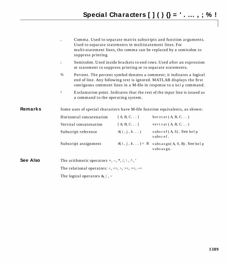
Special Characters [ ] ( ) = ' . ... , ; % !
1389
Remarks Some uses of special characters have M-file function equivalents, as shown:
See Also The arithmetic operators +, –, *, /, \, ^, '
The relational operators: <, <=, >, >=, ==, ~=
The logical operators &, |, ~
, Comma. Used to separate matrix subscripts and function arguments.Used to separate statements in multistatement lines. Formulti-statement lines, the comma can be replaced by a semicolon tosuppress printing.
; Semicolon. Used inside brackets to end rows. Used after an expressionor statement to suppress printing or to separate statements.
% Percent. The percent symbol denotes a comment; it indicates a logicalend of line. Any following text is ignored. MATLAB displays the firstcontiguous comment lines in a M-file in response to a help command.
! Exclamation point. Indicates that the rest of the input line is issued asa command to the operating system.
Horizontal concatenation [A,B,C...] horzcat(A,B,C...)
Vertical concatenation [A;B;C...] vertcat(A,B,C...)
Subscript reference A(i,j,k...) subsref(A,S). See helpsubsref.
Subscript assignment A(i,j,k...)= B subsasgn(A,S,B). See helpsubsasgn.
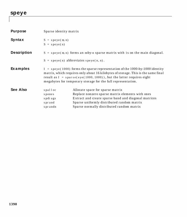
speye
1390
1speyePurpose Sparse identity matrix
Syntax S = speye(m,n)S = speye(n)
Description S = speye(m,n) forms an m-by-n sparse matrix with 1s on the main diagonal.
S = speye(n) abbreviates speye(n,n).
Examples I = speye(1000) forms the sparse representation of the 1000-by-1000 identitymatrix, which requires only about 16 kilobytes of storage. This is the same finalresult as I = sparse(eye(1000,1000)), but the latter requires eightmegabytes for temporary storage for the full representation.
See Also spalloc Allocate space for sparse matrixspones Replace nonzero sparse matrix elements with onesspdiags Extract and create sparse band and diagonal matricessprand Sparse uniformly distributed random matrixsprandn Sparse normally distributed random matrix
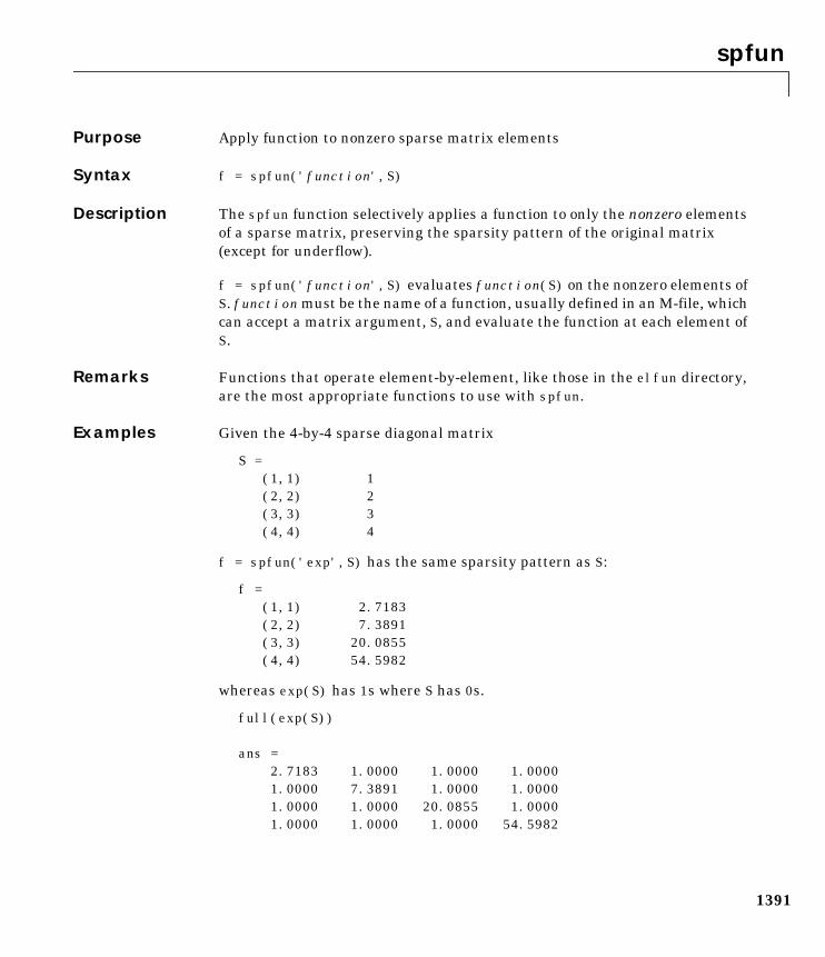
spfun
1391
1spfunPurpose Apply function to nonzero sparse matrix elements
Syntax f = spfun('function',S)
Description The spfun function selectively applies a function to only the nonzero elementsof a sparse matrix, preserving the sparsity pattern of the original matrix(except for underflow).
f = spfun('function',S) evaluates function(S) on the nonzero elements ofS. function must be the name of a function, usually defined in an M-file, whichcan accept a matrix argument, S, and evaluate the function at each element ofS.
Remarks Functions that operate element-by-element, like those in the elfun directory,are the most appropriate functions to use with spfun.
Examples Given the 4-by-4 sparse diagonal matrix
S = (1,1) 1 (2,2) 2 (3,3) 3 (4,4) 4
f = spfun('exp',S) has the same sparsity pattern as S:
f = (1,1) 2.7183 (2,2) 7.3891 (3,3) 20.0855 (4,4) 54.5982
whereas exp(S) has 1s where S has 0s.
full(exp(S))
ans = 2.7183 1.0000 1.0000 1.0000 1.0000 7.3891 1.0000 1.0000 1.0000 1.0000 20.0855 1.0000 1.0000 1.0000 1.0000 54.5982
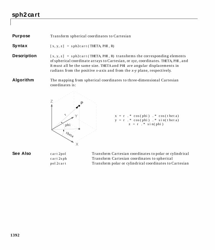
sph2cart
1392
1sph2cartPurpose Transform spherical coordinates to Cartesian
Syntax [x,y,z] = sph2cart(THETA,PHI,R)
Description [x,y,z] = sph2cart(THETA,PHI,R) transforms the corresponding elementsof spherical coordinate arrays to Cartesian, or xyz, coordinates. THETA, PHI, andR must all be the same size. THETA and PHI are angular displacements inradians from the positive x-axis and from the x-y plane, respectively.
Algorithm The mapping from spherical coordinates to three-dimensional Cartesiancoordinates is:
See Also cart2pol Transform Cartesian coordinates to polar or cylindricalcart2sph Transform Cartesian coordinates to sphericalpol2cart Transform polar or cylindrical coordinates to Cartesian
x = r .* cos(phi) .* cos(theta)y = r .* cos(phi) .* sin(theta)
z = r .* sin(phi)
Z
Y
X
theta
P
phi
r
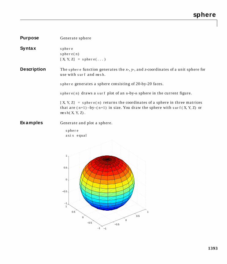
sphere
1393
1spherePurpose Generate sphere
Syntax spheresphere(n)[X,Y,Z] = sphere(...)
Description The sphere function generates the x-, y-, and z-coordinates of a unit sphere foruse with surf and mesh.
sphere generates a sphere consisting of 20-by-20 faces.
sphere(n) draws a surf plot of an n-by-n sphere in the current figure.
[X,Y,Z] = sphere(n) returns the coordinates of a sphere in three matricesthat are (n+1)–by–(n+1) in size. You draw the sphere with surf(X,Y,Z) ormesh(X,Y,Z).
Examples Generate and plot a sphere.
sphereaxis equal
−1
−0.5
0
0.5
1
−1
−0.5
0
0.5
1−1
−0.5
0
0.5
1

sphere
1394
See Also cylinder, axis
spinmap
1395
1spinmapPurpose Spin colormap
Syntax spinmapspinmap(t)spinmap(t,inc)spinmap('inf')
Description The spinmap function shifts the colormap RGB values by some incrementalvalue. For example, if the increment equals 1, color 1 becomes color 2, color 2becomes color 3, etc.
spinmap cyclically rotates the colormap for approximately five seconds usingan incremental value of 2.
spinmap(t) rotates the colormap for approximately 10*t seconds. The amountof time specified by t depends on your hardware configuration (e.g., if you arerunning MATLAB over a network).
spinmap(t,inc) rotates the colormap for approximately 10*t seconds andspecifies an increment inc by which the colormap shifts. When inc is 1, therotation appears smoother than the default (i.e., 2). Increments greater than 2are less smooth than the default. A negative increment (e.g., –2) rotates thecolormap in a negative direction.
spinmap('inf') rotates the colormap for an infinite amount of time. To breakthe loop, press Ctrl-C .
See Also colormap
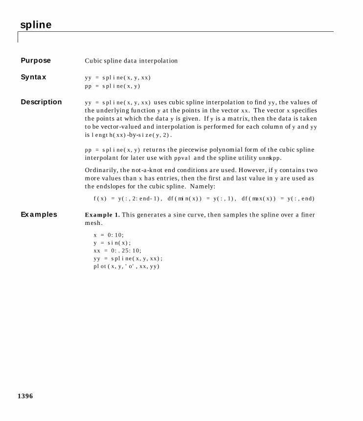
spline
1396
1splinePurpose Cubic spline data interpolation
Syntax yy = spline(x,y,xx)pp = spline(x,y)
Description yy = spline(x,y,xx) uses cubic spline interpolation to find yy, the values ofthe underlying function y at the points in the vector xx. The vector x specifiesthe points at which the data y is given. If y is a matrix, then the data is takento be vector-valued and interpolation is performed for each column of y and yyis length(xx)-by-size(y,2).
pp = spline(x,y) returns the piecewise polynomial form of the cubic splineinterpolant for later use with ppval and the spline utility unmkpp.
Ordinarily, the not-a-knot end conditions are used. However, if y contains twomore values than x has entries, then the first and last value in y are used asthe endslopes for the cubic spline. Namely:
f(x) = y(:,2:end-1), df(min(x)) = y(:,1), df(max(x)) = y(:,end)
Examples Example 1. This generates a sine curve, then samples the spline over a finermesh.
x = 0:10;y = sin(x);xx = 0:.25:10;yy = spline(x,y,xx);plot(x,y,'o',xx,yy)
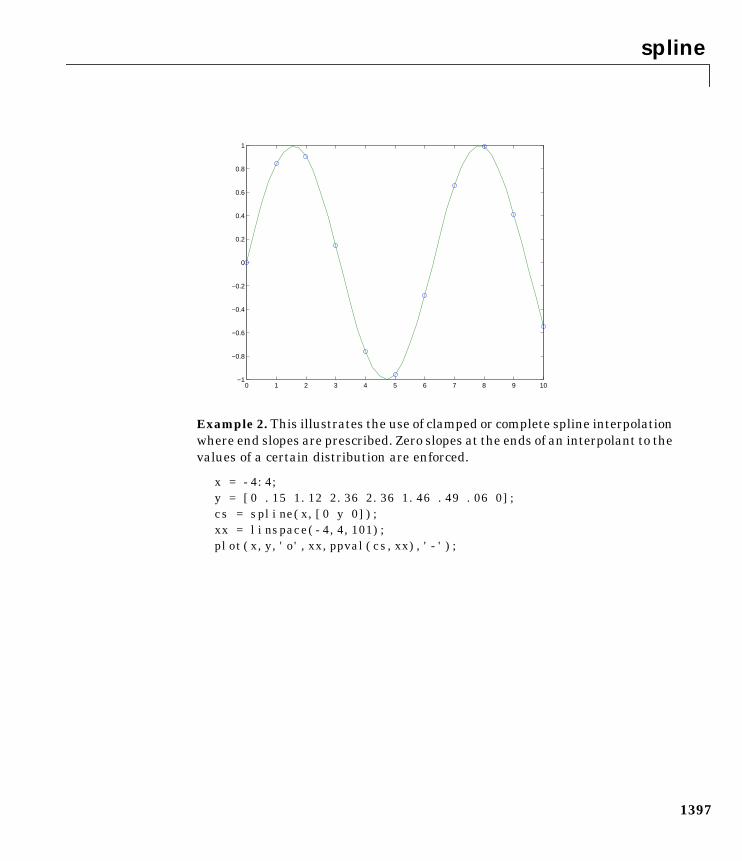
spline
1397
Example 2. This illustrates the use of clamped or complete spline interpolationwhere end slopes are prescribed. Zero slopes at the ends of an interpolant to thevalues of a certain distribution are enforced.
x = -4:4;y = [0 .15 1.12 2.36 2.36 1.46 .49 .06 0];cs = spline(x,[0 y 0]);xx = linspace(-4,4,101);plot(x,y,'o',xx,ppval(cs,xx),'-');
0 1 2 3 4 5 6 7 8 9 10−1
−0.8
−0.6
−0.4
−0.2
0
0.2
0.4
0.6
0.8
1
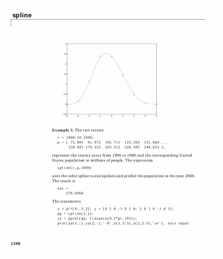
spline
1398
Example 3. The two vectors
t = 1900:10:1990;p = [ 75.995 91.972 105.711 123.203 131.669 ...
150.697 179.323 203.212 226.505 249.633 ];
represent the census years from 1900 to 1990 and the corresponding UnitedStates population in millions of people. The expression
spline(t,p,2000)
uses the cubic spline to extrapolate and predict the population in the year 2000.The result is
ans =270.6060
The statements
x = pi*[0:.5:2]; y = [0 1 0 -1 0 1 0; 1 0 1 0 -1 0 1];pp = spline(x,y);yy = ppval(pp, linspace(0,2*pi,101));plot(yy(1,:),yy(2,:),'-b',y(1,2:5),y(2,2:5),'or'), axis equal
−4 −3 −2 −1 0 1 2 3 4−0.5
0
0.5
1
1.5
2
2.5
3
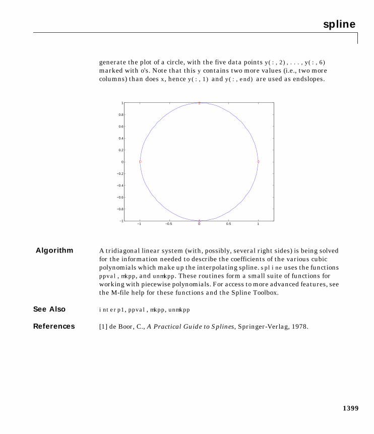
spline
1399
generate the plot of a circle, with the five data points y(:,2),...,y(:,6)marked with o's. Note that this y contains two more values (i.e., two morecolumns) than does x, hence y(:,1) and y(:,end) are used as endslopes.
Algorithm A tridiagonal linear system (with, possibly, several right sides) is being solvedfor the information needed to describe the coefficients of the various cubicpolynomials which make up the interpolating spline. spline uses the functionsppval, mkpp, and unmkpp. These routines form a small suite of functions forworking with piecewise polynomials. For access to more advanced features, seethe M-file help for these functions and the Spline Toolbox.
See Also interp1, ppval, mkpp, unmkpp
References [1] de Boor, C., A Practical Guide to Splines, Springer-Verlag, 1978.
−1 −0.5 0 0.5 1−1
−0.8
−0.6
−0.4
−0.2
0
0.2
0.4
0.6
0.8
1
spones
1400
1sponesPurpose Replace nonzero sparse matrix elements with ones
Syntax R = spones(S)
Description R = spones(S) generates a matrix R with the same sparsity structure as S, butwith 1’s in the nonzero positions.
Examples c = sum(spones(S)) is the number of nonzeros in each column.
r = sum(spones(S'))' is the number of nonzeros in each row.
sum(c) and sum(r) are equal, and are equal to nnz(S).
See Also nnz Number of nonzero matrix elementsspalloc Allocate space for sparse matrixspfun Apply function to nonzero sparse matrix elements
spparms
1401
1spparmsPurpose Set parameters for sparse matrix routines
Syntax spparms('key',value)spparmsvalues = spparms[keys,values] = spparmsspparms(values)value = spparms('key')spparms('default')spparms('tight')
Description spparms('key',value) sets one or more of the tunable parameters used in thesparse linear equation operators, \ and /, and the minimum degree orderings,colmmd and symmmd. In ordinary use, you should never need to deal with thisfunction.
The meanings of the key parameters are
'spumoni' Sparse Monitor flag.0 produces no diagnostic output, the default.1 produces information about choice of algorithm based onmatrix structure, and about storage allocation.2 also produces very detailed information about the minimumdegree algorithms.
'thr_rel','thr_abs'
Minimum degree threshold is thr_rel*mindegree+thr_abs.
'exact_d' Nonzero to use exact degrees in minimum degree. Zero to useapproximate degrees.
'supernd' If positive, minimum degree amalgamates the supernodesevery supernd stages.
'rreduce' If positive, minimum degree does row reduction every rreducestages.
'wh_frac' Rows with density > wh_frac are ignored in colmmd.
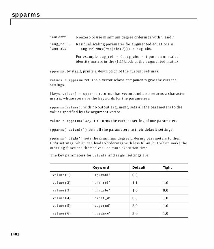
spparms
1402
spparms, by itself, prints a description of the current settings.
values = spparms returns a vector whose components give the currentsettings.
[keys,values] = spparms returns that vector, and also returns a charactermatrix whose rows are the keywords for the parameters.
spparms(values), with no output argument, sets all the parameters to thevalues specified by the argument vector.
value = spparms('key') returns the current setting of one parameter.
spparms('default') sets all the parameters to their default settings.
spparms('tight') sets the minimum degree ordering parameters to theirtight settings, which can lead to orderings with less fill-in, but which make theordering functions themselves use more execution time.
The key parameters for default and tight settings are
'autommd' Nonzero to use minimum degree orderings with \ and /.
'aug_rel','aug_abs'
Residual scaling parameter for augmented equations isaug_rel∗max(max(abs(A))) + aug_abs.
For example, aug_rel = 0, aug_abs = 1 puts an unscaledidentity matrix in the (1,1) block of the augmented matrix.
Keyword Default Tight
values(1) 'spumoni' 0.0
values(2) 'thr_rel' 1.1 1.0
values(3) 'thr_abs' 1.0 0.0
values(4) 'exact_d' 0.0 1.0
values(5) 'supernd' 3.0 1.0
values(6) 'rreduce' 3.0 1.0
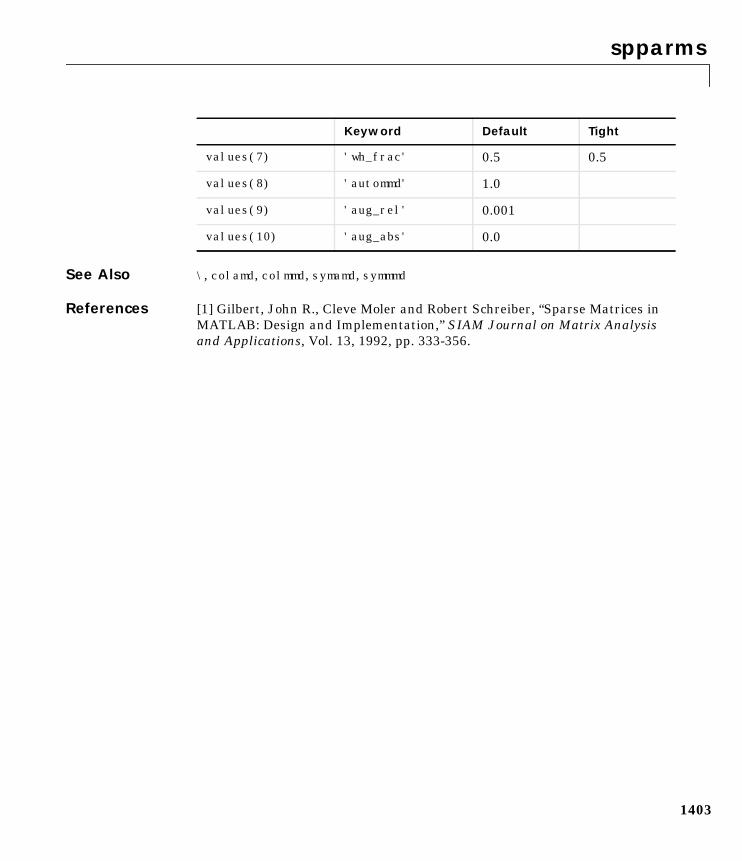
spparms
1403
See Also \, colamd, colmmd, symamd, symmmd
References [1] Gilbert, John R., Cleve Moler and Robert Schreiber, “Sparse Matrices inMATLAB: Design and Implementation,” SIAM Journal on Matrix Analysisand Applications, Vol. 13, 1992, pp. 333-356.
values(7) 'wh_frac' 0.5 0.5
values(8) 'autommd' 1.0
values(9) 'aug_rel' 0.001
values(10) 'aug_abs' 0.0
Keyword Default Tight
sprand
1404
1sprandPurpose Sparse uniformly distributed random matrix
Syntax R = sprand(S)R = sprand(m,n,density)R = sprand(m,n,density,rc)
Description R = sprand(S) has the same sparsity structure as S, but uniformly distributedrandom entries.
R = sprand(m,n,density) is a random, m-by-n, sparse matrix withapproximately density∗m∗n uniformly distributed nonzero entries(0 ≤ density ≤ 1).
R = sprand(m,n,density,rc) also has reciprocal condition numberapproximately equal to rc. R is constructed from a sum of matrices of rank one.
If rc is a vector of length lr, where lr ≤ min(m,n), then R has rc as its first lrsingular values, all others are zero. In this case, R is generated by random planerotations applied to a diagonal matrix with the given singular values. It has agreat deal of topological and algebraic structure.
See Also sprandn Sparse normally distributed random matrixsprandsym Sparse symmetric random matrix
sprandn
1405
1sprandnPurpose Sparse normally distributed random matrix
Syntax R = sprandn(S)R = sprandn(m,n,density)R = sprandn(m,n,density,rc)
Description R = sprandn(S) has the same sparsity structure as S, but normally distributedrandom entries with mean 0 and variance 1.
R = sprandn(m,n,density) is a random, m-by-n, sparse matrix withapproximately density∗m∗n normally distributed nonzero entries(0 ≤ density ≤ 1).
R = sprandn(m,n,density,rc) also has reciprocal condition numberapproximately equal to rc. R is constructed from a sum of matrices of rank one.
If rc is a vector of length lr, where lr ≤ min(m,n), then R has rc as its first lrsingular values, all others are zero. In this case, R is generated by random planerotations applied to a diagonal matrix with the given singular values. It has agreat deal of topological and algebraic structure.
See Also sprand Sparse uniformly distributed random matrixsprandn Sparse normally distributed random matrix
sprandsym
1406
1sprandsymPurpose Sparse symmetric random matrix
Syntax R = sprandsym(S)R = sprandsym(n,density)R = sprandsym(n,density,rc)R = sprandsym(n,density,rc,kind)
Description R = sprandsym(S) returns a symmetric random matrix whose lower triangleand diagonal have the same structure as S. Its elements are normallydistributed, with mean 0 and variance 1.
R = sprandsym(n,density) returns a symmetric random, n-by-n, sparsematrix with approximately density∗n∗n nonzeros; each entry is the sum of oneor more normally distributed random samples, and (0 ≤ density ≤ 1).
R = sprandsym(n,density,rc) returns a matrix with a reciprocal conditionnumber equal to rc. The distribution of entries is nonuniform; it is roughlysymmetric about 0; all are in .
If rc is a vector of length n, then R has eigenvalues rc. Thus, if rc is a positive(nonnegative) vector then R is a positive definite matrix. In either case, R isgenerated by random Jacobi rotations applied to a diagonal matrix with thegiven eigenvalues or condition number. It has a great deal of topological andalgebraic structure.
R = sprandsym(n,density,rc,kind) returns a positive definite matrix.Argument kind can be:
• 1 to generate R by random Jacobi rotation of a positive definite diagonalmatrix. R has the desired condition number exactly.
• 2 to generate an R that is a shifted sum of outer products. R has the desiredcondition number only approximately, but has less structure.
• 3 to generate an R that has the same structure as the matrix S andapproximate condition number 1/rc. density is ignored.
See Also sprand Sparse uniformly distributed random matrixsprandn Sparse normally distributed random matrix
1 1,–[ ]
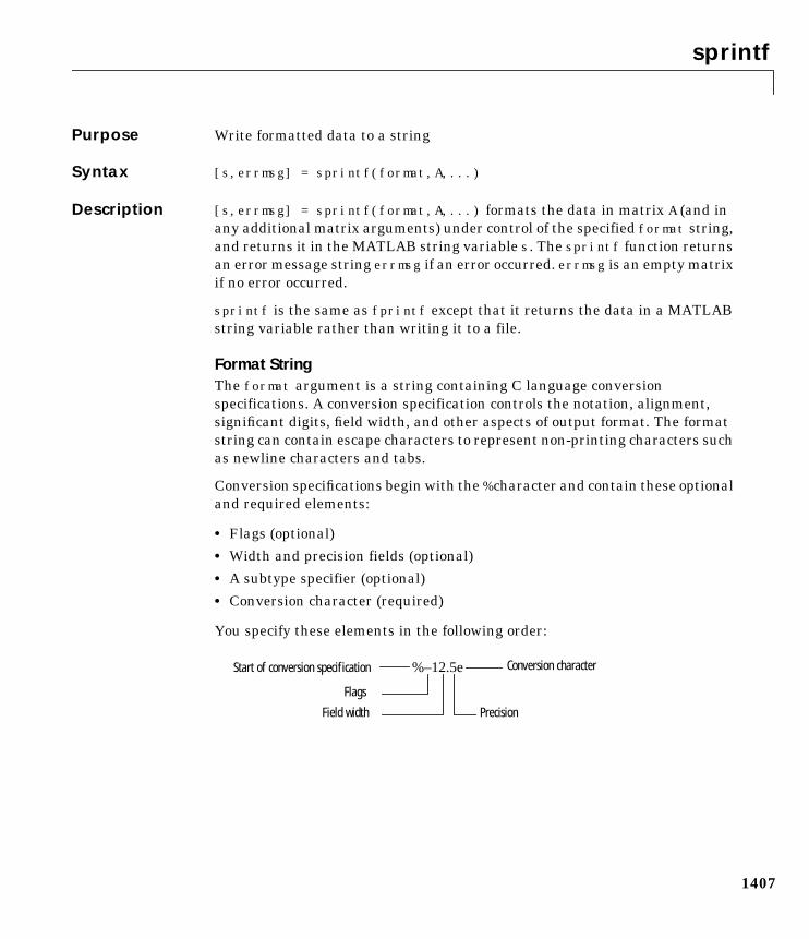
sprintf
1407
1sprintfPurpose Write formatted data to a string
Syntax [s,errmsg] = sprintf(format,A,...)
Description [s,errmsg] = sprintf(format,A,...) formats the data in matrix A (and inany additional matrix arguments) under control of the specified format string,and returns it in the MATLAB string variable s. The sprintf function returnsan error message string errmsg if an error occurred. errmsg is an empty matrixif no error occurred.
sprintf is the same as fprintf except that it returns the data in a MATLABstring variable rather than writing it to a file.
Format StringThe format argument is a string containing C language conversionspecifications. A conversion specification controls the notation, alignment,significant digits, field width, and other aspects of output format. The formatstring can contain escape characters to represent non-printing characters suchas newline characters and tabs.
Conversion specifications begin with the % character and contain these optionaland required elements:
• Flags (optional)
• Width and precision fields (optional)
• A subtype specifier (optional)
• Conversion character (required)
You specify these elements in the following order:
%–12.5eStart of conversion specif ication
Field width
Conversion character
Flags
Precision
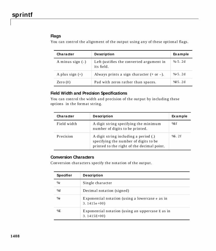
sprintf
1408
FlagsYou can control the alignment of the output using any of these optional flags.
Field Width and Precision SpecificationsYou can control the width and precision of the output by including theseoptions in the format string.
Conversion CharactersConversion characters specify the notation of the output.
Character Description Example
A minus sign (–) Left-justifies the converted argument inits field.
%–5.2d
A plus sign (+) Always prints a sign character (+ or –). %+5.2d
Zero (0) Pad with zeros rather than spaces. %05.2d
Character Description Example
Field width A digit string specifying the minimumnumber of digits to be printed.
%6f
Precision A digit string including a period (.)specifying the number of digits to beprinted to the right of the decimal point.
%6.2f
Specifier Description
%c Single character
%d Decimal notation (signed)
%e Exponential notation (using a lowercase e as in3.1415e+00)
%E Exponential notation (using an uppercase E as in3.1415E+00)
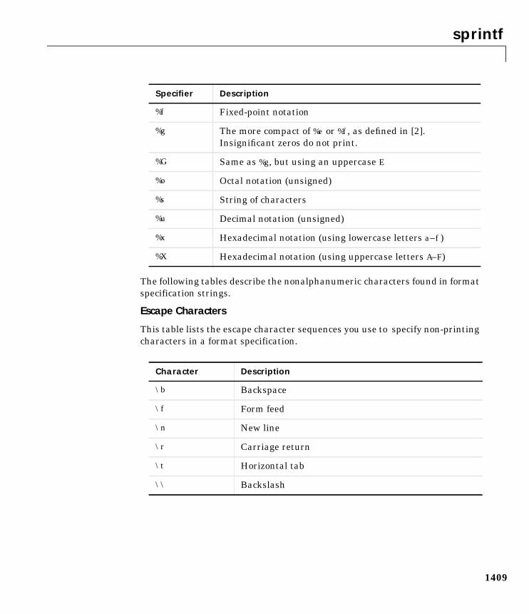
sprintf
1409
The following tables describe the nonalphanumeric characters found in formatspecification strings.
Escape Characters
This table lists the escape character sequences you use to specify non-printingcharacters in a format specification.
%f Fixed-point notation
%g The more compact of %e or %f, as defined in [2].Insignificant zeros do not print.
%G Same as %g, but using an uppercase E
%o Octal notation (unsigned)
%s String of characters
%u Decimal notation (unsigned)
%x Hexadecimal notation (using lowercase letters a–f)
%X Hexadecimal notation (using uppercase letters A–F)
Character Description
\b Backspace
\f Form feed
\n New line
\r Carriage return
\t Horizontal tab
\\ Backslash
Specifier Description
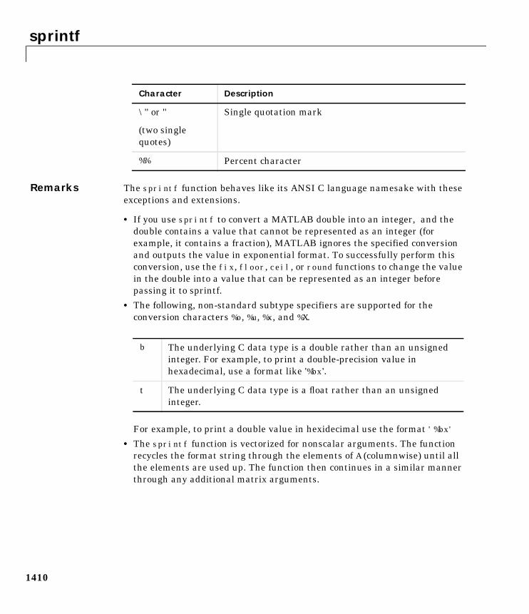
sprintf
1410
Remarks The sprintf function behaves like its ANSI C language namesake with theseexceptions and extensions.
• If you use sprintf to convert a MATLAB double into an integer, and thedouble contains a value that cannot be represented as an integer (forexample, it contains a fraction), MATLAB ignores the specified conversionand outputs the value in exponential format. To successfully perform thisconversion, use the fix, floor, ceil, or round functions to change the valuein the double into a value that can be represented as an integer beforepassing it to sprintf.
• The following, non-standard subtype specifiers are supported for theconversion characters %o, %u, %x, and %X.
For example, to print a double value in hexidecimal use the format '%bx'
• The sprintf function is vectorized for nonscalar arguments. The functionrecycles the format string through the elements of A (columnwise) until allthe elements are used up. The function then continues in a similar mannerthrough any additional matrix arguments.
\'' or ''
(two singlequotes)
Single quotation mark
%% Percent character
Character Description
b The underlying C data type is a double rather than an unsignedinteger. For example, to print a double-precision value inhexadecimal, use a format like '%bx'.
t The underlying C data type is a float rather than an unsignedinteger.
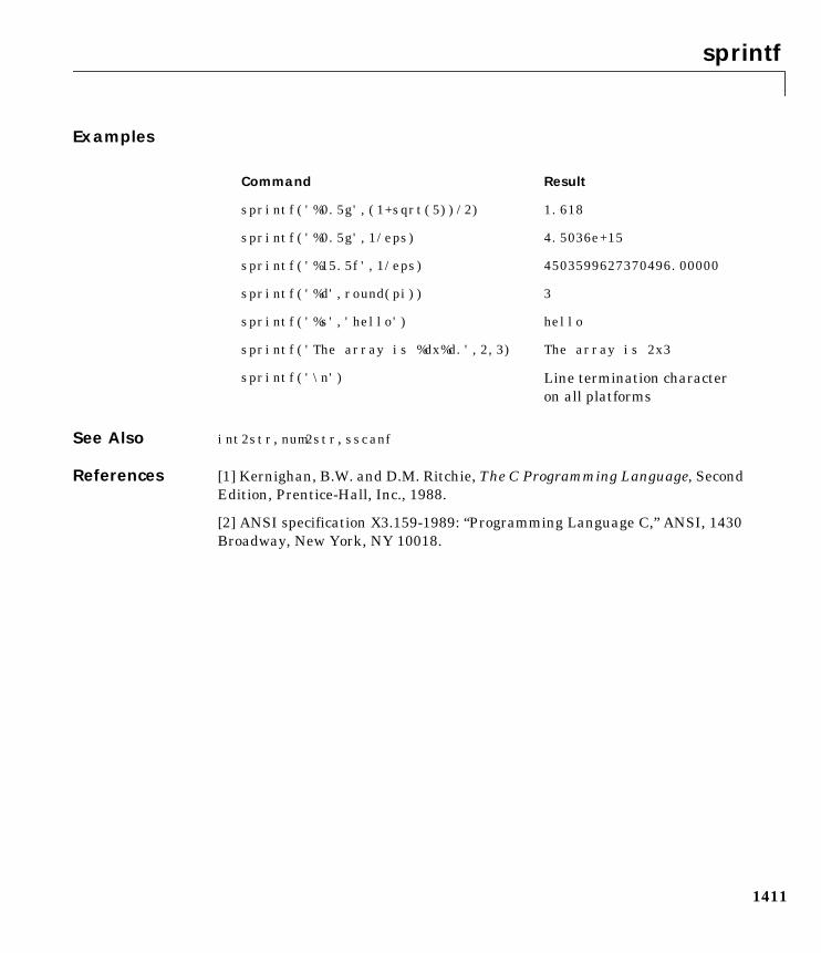
sprintf
1411
Examples
See Also int2str, num2str, sscanf
References [1] Kernighan, B.W. and D.M. Ritchie, The C Programming Language, SecondEdition, Prentice-Hall, Inc., 1988.
[2] ANSI specification X3.159-1989: “Programming Language C,” ANSI, 1430Broadway, New York, NY 10018.
Command Result
sprintf('%0.5g',(1+sqrt(5))/2) 1.618
sprintf('%0.5g',1/eps) 4.5036e+15
sprintf('%15.5f',1/eps) 4503599627370496.00000
sprintf('%d',round(pi)) 3
sprintf('%s','hello') hello
sprintf('The array is %dx%d.',2,3) The array is 2x3
sprintf('\n') Line termination characteron all platforms
spy
1412
1spyPurpose Visualize sparsity pattern
Syntax spy(S)spy(S,markersize)spy(S,'LineSpec')spy(S,'LineSpec',markersize)
Description spy(S) plots the sparsity pattern of any matrix S.
spy(S,marksize), where markersize is an integer, plots the sparsity patternusing markers of the specified point size.
spy(S,'LineSpec'), where LineSpec is a string, uses the specified plot markertype and color.
spy(S,'LineSpec',markersize) uses the specified type, color, and size for theplot markers.
S is usually a sparse matrix, but full matrices are acceptable, in which case thelocations of the nonzero elements are plotted.
spy replaces format +, which takes much more space to display essentially thesame information.
See Also find, gplot, LineSpec, symamd, symmmd, symrcm
sqrt
1413
1sqrtPurpose Square root
Syntax B = sqrt(X)
Description B = sqrt(X) returns the square root of each element of the array X. For theelements of X that are negative or complex, sqrt(X) produces complex results.
Remarks See sqrtm for the matrix square root.
Examples sqrt((-2:2)')ans =
0 + 1.4142i0 + 1.0000i0
1.00001.4142
See Also
sqrtm
1414
1sqrtmPurpose Matrix square root
Syntax X = sqrtm(A)[X,resnorm] = sqrtm(A)[X,alpha,condest] = sqrtm(A)
Description X = sqrtm(A) is the principal square root of the matrix A, i.e. X*X = A.
X is the unique square root for which every eigenvalue has nonnegative realpart. If A has any eigenvalues with negative real parts then a complex resultis produced. If A is singular then A may not have a square root. A warning isprinted if exact singularity is detected.
[X, resnorm] = sqrtm(A) does not print any warning, and returns theresidual, norm(A-X^2,'fro')/norm(A,'fro').
[X, alpha, condest] = sqrtm(A) returns a stability factor alpha and anestimate condest of the matrix square root condition number of X. The residualnorm(A-X^2,'fro')/norm(A,'fro') is bounded approximately byn*alpha*eps and the Frobenius norm relative error in X is boundedapproximately by n*alpha*condest*eps, where n = max(size(A)).
Remarks If X is real, symmetric and positive definite, or complex, Hermitian and positivedefinite, then so is the computed matrix square root.
Some matrices, like X = [0 1; 0 0], do not have any square roots, real orcomplex, and sqrtm cannot be expected to produce one.
Examples Example 1. A matrix representation of the fourth difference operator is
X =5 -4 1 0 0
-4 6 -4 1 01 -4 6 -4 10 1 -4 6 -40 0 1 -4 5
This matrix is symmetric and positive definite. Its unique positive definitesquare root, Y = sqrtm(X), is a representation of the second differenceoperator.
sqrtm
1415
Y =2 -1 -0 -0 -0
-1 2 -1 0 -0 0 -1 2 -1 0-0 0 -1 2 -1-0 -0 -0 -1 2
Example 2. The matrix
X =7 10
15 22
has four square roots. Two of them are
Y1 =1.5667 1.74082.6112 4.1779
and
Y2 =1 23 4
The other two are -Y1 and -Y2. All four can be obtained from the eigenvaluesand vectors of X.
[V,D] = eig(X);D =
0.1386 00 28.8614
The four square roots of the diagonal matrix D result from the four choices ofsign in
S =±0.3723 0
0 ±5.3723
All four Ys are of the form
Y = V*S/V
sqrtm
1416
The sqrtm function chooses the two plus signs and produces Y1, even though Y2is more natural because its entries are integers.
See Also expm Matrix exponentialfunm Evaluate functions of a matrixlogm Matrix logarithm
squeeze
1417
1squeezePurpose Remove singleton dimensions
Syntax B = squeeze(A)
Description B = squeeze(A) returns an array B with the same elements as A, but with allsingleton dimensions removed. A singleton dimension is any dimension forwhichsize(A,dim) = 1.
Examples Consider the 2-by-1-by-3 array Y = rand(2,1,3). This array has a singletoncolumn dimension — that is, there’s only one column per page.
Y =
Y(:,:,1) = Y(:,:,2) = 0.5194 0.0346 0.8310 0.0535
Y(:,:,3) = 0.5297 0.6711
The command Z = squeeze(Y) yields a 2-by-3 matrix:
Z = 0.5194 0.0346 0.5297 0.8310 0.0535 0.6711
See Also reshape Reshape arrayshiftdim Shift dimensions
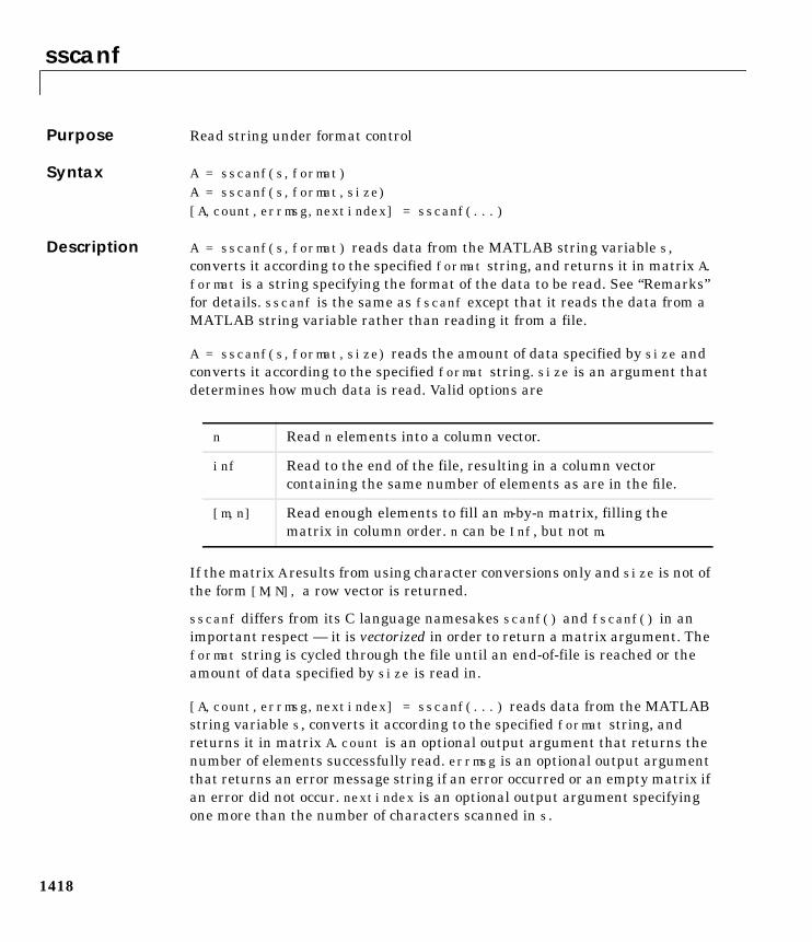
sscanf
1418
1sscanfPurpose Read string under format control
Syntax A = sscanf(s,format)A = sscanf(s,format,size)[A,count,errmsg,nextindex] = sscanf(...)
Description A = sscanf(s,format) reads data from the MATLAB string variable s,converts it according to the specified format string, and returns it in matrix A.format is a string specifying the format of the data to be read. See “Remarks”for details. sscanf is the same as fscanf except that it reads the data from aMATLAB string variable rather than reading it from a file.
A = sscanf(s,format,size) reads the amount of data specified by size andconverts it according to the specified format string. size is an argument thatdetermines how much data is read. Valid options are
If the matrix A results from using character conversions only and size is not ofthe form [M,N], a row vector is returned.
sscanf differs from its C language namesakes scanf() and fscanf() in animportant respect — it is vectorized in order to return a matrix argument. Theformat string is cycled through the file until an end-of-file is reached or theamount of data specified by size is read in.
[A,count,errmsg,nextindex] = sscanf(...) reads data from the MATLABstring variable s, converts it according to the specified format string, andreturns it in matrix A. count is an optional output argument that returns thenumber of elements successfully read. errmsg is an optional output argumentthat returns an error message string if an error occurred or an empty matrix ifan error did not occur. nextindex is an optional output argument specifyingone more than the number of characters scanned in s.
n Read n elements into a column vector.
inf Read to the end of the file, resulting in a column vectorcontaining the same number of elements as are in the file.
[m,n] Read enough elements to fill an m-by-n matrix, filling thematrix in column order. n can be Inf, but not m.
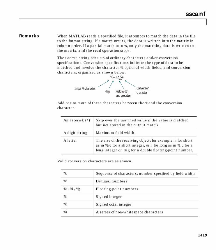
sscanf
1419
Remarks When MATLAB reads a specified file, it attempts to match the data in the fileto the format string. If a match occurs, the data is written into the matrix incolumn order. If a partial match occurs, only the matching data is written tothe matrix, and the read operation stops.
The format string consists of ordinary characters and/or conversionspecifications. Conversion specifications indicate the type of data to bematched and involve the character %, optional width fields, and conversioncharacters, organized as shown below:
Add one or more of these characters between the % and the conversioncharacter.
Valid conversion characters are as shown.
An asterisk (*) Skip over the matched value if the value is matchedbut not stored in the output matrix.
A digit string Maximum field width.
A letter The size of the receiving object; for example, h for shortas in %hd for a short integer, or l for long as in %ld for along integer or %lg for a double floating-point number.
%c Sequence of characters; number specified by field width
%d Decimal numbers
%e, %f, %g Floating-point numbers
%i Signed integer
%o Signed octal integer
%s A series of non-whitespace characters
%–12.5e
Initial % characterField widthand precision
ConversioncharacterFlag
sscanf
1420
If %s is used, an element read may use several MATLAB matrix elements, eachholding one character. Use %c to read space characters, or %s to skip all whitespace.
Mixing character and numeric conversion specifications cause the resultingmatrix to be numeric and any characters read to appear as their ASCII values,one character per MATLAB matrix element.
For more information about format strings, refer to the scanf() and fscanf()routines in a C language reference manual.
Examples The statements
s = '2.7183 3.1416';A = sscanf(s,'%f')
create a two-element vector containing poor approximations to e and pi.
See Also eval, sprintf, textread
%u Signed decimal integer
%x Signed hexadecimal integer
[...] Sequence of characters (scanlist)
stairs
1421
1stairsPurpose Stairstep plot
Syntax stairs(Y)stairs(X,Y)stairs(...,LineSpec)[xb,yb] = stairs(Y)[xb,yb] = stairs(X,Y)
Description Stairstep plots are useful for drawing time-history plots of digitally sampleddata systems.
stairs(Y) draws a stairstep plot of the elements of Y. When Y is a vector, thex-axis scale ranges from 1 to size(Y). When Y is a matrix, the x-axis scaleranges from 1 to the number of rows in Y.
stairs(X,Y) plots X versus the columns of Y. X and Y are vectors of the samesize or matrices of the same size. Additionally, X can be a row or a columnvector, and Y a matrix with length(X) rows.
stairs(...,LineSpec) specifies a line style, marker symbol, and color for theplot (see LineSpec for more information).
[xb,yb] = stairs(Y) and [xb,yb] = stairs(x,Y) do not draw graphs, butreturn vectors xb and yb such that plot(xb,yb) plots the stairstep graph.
Examples Create a stairstep plot of a sine wave.
x = 0:.25:10;stairs(x,sin(x))
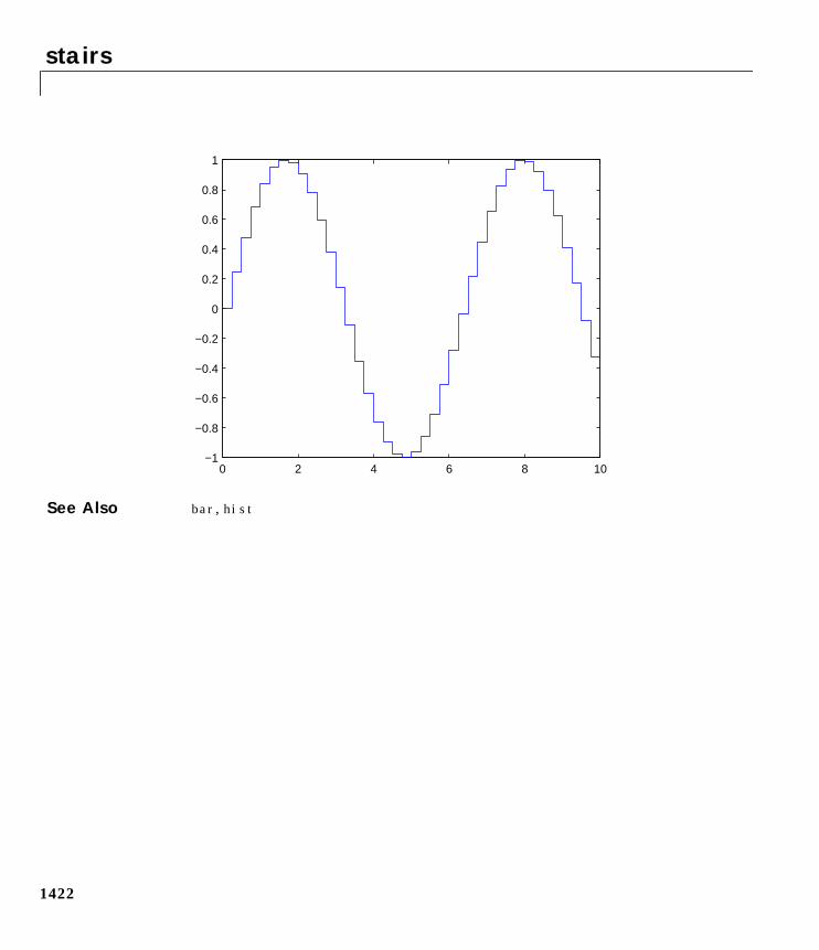
stairs
1422
See Also bar, hist
0 2 4 6 8 10−1
−0.8
−0.6
−0.4
−0.2
0
0.2
0.4
0.6
0.8
1
startup
1423
1startupPurpose MATLAB startup M-file
Description startup automatically executes the master M-file matlabrc.m and, if itexists, startup.m, when MATLAB starts. On multiuser or networked systems,matlabrc.m is reserved for use by the system manager. The file matlabrc.minvokes the file startup.m if it exists on MATLAB’s search path.
You can create a startup file in your own MATLAB directory. The file caninclude physical constants, handle graphics defaults, engineering conversionfactors, or anything else you want predefined in your workspace.
There are other way to predefine aspects of MATLAB. See “Startup Options”and “Setting Preferences”.
Algorithm Only matlabrc.m is actually invoked by MATLAB at startup. However,matlabrc.m contains the statements
if exist('startup')==2startup
end
that invoke startup.m. You can extend this process to create additional startupM-files, if required.
See Also matlabrc, quit
std
1424
1stdPurpose Standard deviation
Syntax s = std(X)s = std(X,flag)s = std(X,flag,dim)
Definition There are two common textbook definitions for the standard deviation s of adata vector X:
where
and n is the number of elements in the sample. The two forms of the equationdiffer only in versus in the divisor.
Description s = std(X), where X is a vector, returns the standard deviation using (1)above. If X is a random sample of data from a normal distribution, s2 is the bestunbiased estimate of its variance.
If X is a matrix, std(X) returns a row vector containing the standard deviationof the elements of each column of X. If X is a multidimensional array, std(X) isthe standard deviation of th elements along the first nonsingleton dimension ofX.
s = std(X,flag) for flag = 0, is the same as std(X). For flag = 1, std(X,1)returns the standard deviation using (2) above, producing the second momentof the sample about its mean.
s = std(X,flag,dim) computes the standard deviations along the dimensionof X specified by scalar dim.
(1) s 1n 1–------------- xi x–( )2
i 1=
n
∑ 1
2---
= and (2) s 1n--- xi x–( )2
i 1=
n
∑ 1
2---
=
x 1n--- xi
i 1=
n
∑=
n 1– n
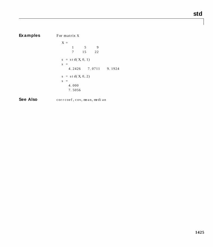
std
1425
Examples For matrix X
X =1 5 9
7 15 22
s = std(X,0,1)s =
4.2426 7.0711 9.1924
s = std(X,0,2)s =
4.0007.5056
See Also corrcoef, cov, mean, median
stem
1426
1stemPurpose Plot discrete sequence data
Syntax stem(Y)stem(X,Y)stem(...,'fill')stem(...,LineSpec)h = stem(...)
Description A two-dimensional stem plot displays data as lines extending from the x-axis.A circle (the default) or other marker whose y-position represents the datavalue terminates each stem.
stem(Y) plots the data sequence Y as stems that extend from equally spacedand automatically generated values along the x-axis. When Y is a matrix, stemplots all elements in a row against the same x value.
stem(X,Y) plots X versus the columns of Y. X and Y are vectors or matrices ofthe same size. Additionally, X can be a row or a column vector and Y a matrixwith length(X) rows.
stem(...,'fill') specifies whether to color the circle at the end of the stem.
stem(...,LineSpec) specifies the line style, marker symbol, and color for thestem plot. See LineSpec for more information.
h = stem(...) returns handles to line graphics objects.
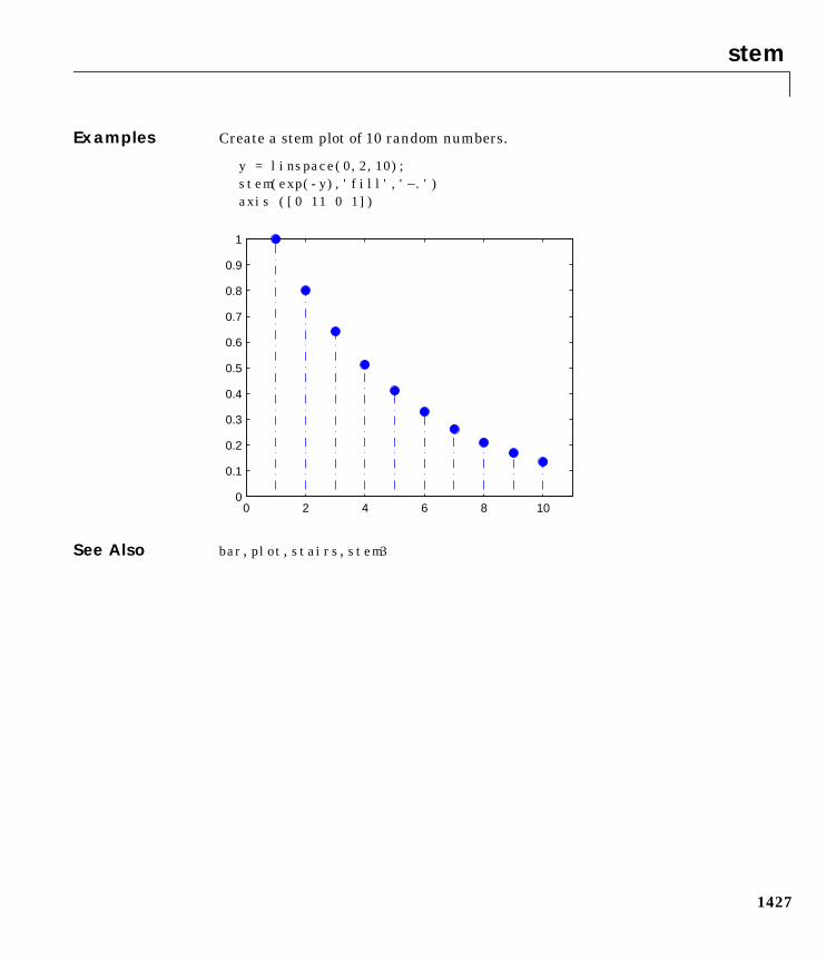
stem
1427
Examples Create a stem plot of 10 random numbers.
y = linspace(0,2,10);stem(exp(-y),'fill','–.')axis ([0 11 0 1])
See Also bar, plot, stairs, stem3
0 2 4 6 8 100
0.1
0.2
0.3
0.4
0.5
0.6
0.7
0.8
0.9
1
stem3
1428
1stem3Purpose Plot three-dimensional discrete sequence data
Syntax stem3(Z)stem3(X,Y,Z)stem3(...,'fill')stem3(...,LineSpec)h = stem3(...)
Description Three-dimensional stem plots display lines extending from the xy-plane. Acircle (the default) or other marker symbol whose z-position represents thedata value terminates each stem.
stem3(Z) plots the data sequence Z as stems that extend from the xy-plane.x and y are generated automatically. When Z is a row vector, stem3 plots allelements at equally spaced x values against the same y value. When Z is acolumn vector, stem3 plots all elements at equally spaced y values against thesame x value.
stem3(X,Y,Z) plots the data sequence Z at values specified by X and Y. X, Y, andZ must all be vectors or matrices of the same size.
stem3(...,'fill') specifies whether to color the interior of the circle at theend of the stem.
stem3(...,LineSpec) specifies the line style, marker symbol, and color for thestems. See LineSpec for more information.
h = stem3(...) returns handles to line graphics objects.
Examples Create a three-dimensional stem plot to visualize a function of two variables.
X = linspace(0,1,10);Y = X./2;Z = sin(X) + cos(Y);stem3(X,Y,Z,'fill')view(-25,30)
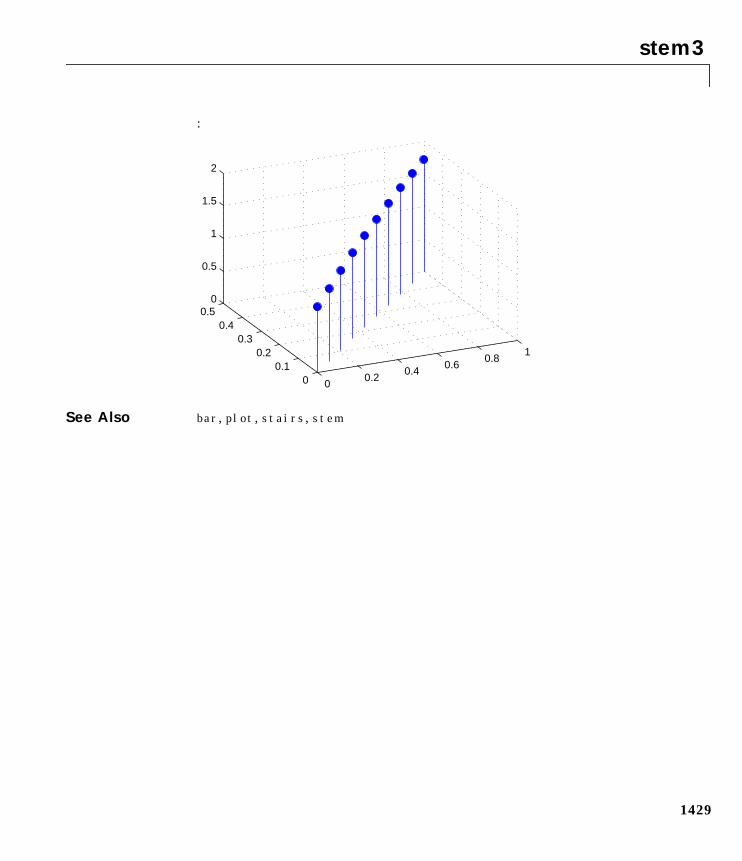
stem3
1429
:
See Also bar, plot, stairs, stem
00.2
0.40.6
0.81
00.1
0.20.3
0.40.5
0
0.5
1
1.5
2
stopasync
1430
1stopasyncPurpose Stop asynchronous read and write operations
Syntax stopasync(obj)
Arguments
Description stopasync(obj) stops any asynchronous read or write operation that is inprogress for obj.
Remarks You can write data asynchronously using the fprintf or fwrite functions. Youcan read data asynchronously using the readasync function, or by configuringthe ReadAsyncMode property to continuous. In-progress asynchronousoperations are indicated by the TransferStatus property.
If obj is an array of serial port objects and one of the objects cannot be stopped,the remaining objects in the array are stopped and a warning is returned. Afteran object stops:
• Its TransferStatus property is configured to idle.
• Its ReadAsyncMode property is configured to manual.
• The data in its output buffer is flushed.
Data in the input buffer is not flushed. You can return this data to theMATLAB workspace using any of the synchronous read functions. If youexecute the readasync function, or configure the ReadAsyncMode property tocontinuous, then the new data is appended to the existing data in the inputbuffer.
See Also Functionsfprintf, fwrite, readasync
PropertiesReadAsyncMode, TransferStatus
obj A serial port object or an array of serial port objects.
str2double
1431
1str2doublePurpose Convert string to double-precision value
Syntax x = str2double('str')X = str2double(C)
Description X = str2double('str') converts the string str, which should be an ASCIIcharacter representation of a real or complex scalar value, to MATLAB'sdouble-precision representation. The string may contain digits, a comma(thousands separator), a decimal point, a leading + or - sign, an e preceeding apower of 10 scale factor, and an i for a complex unit.
If str does not represent a valid scalar value, str2double returns NaN.
X = str2double(C) converts the strings in the cell array of strings C todouble-precision. The matrix X returned will be the same size as C.
Examples Here are some valid str2double conversions.
str2double('123.45e7')str2double('123 + 45i')str2double('3.14159')str2double('2.7i - 3.14')str2double('2.71' '3.1415')str2double('1,200.34')
See Also char, hex2num, num2str, str2num
str2func
1432
1str2funcPurpose Constructs a function handle from a function name string
Syntax fhandle = str2func('str')
Description str2func(‘str’) constructs a function handle, fhandle, for the functionnamed in the string, 'str'.
You can create a function handle using either the @function syntax or thestr2func command. You can also perform this operation on a cell array ofstrings. In this case, an array of function handles is returned.
Examples To create a function handle from the function name, 'humps'
fhandle = str2func('humps')fhandle = @humps
To create an array of function handles from a cell array of function names
fh_array = str2func('sin' 'cos' 'tan')fh_array = @sin @cos @tan
See Also function_handle, func2str, functions
str2mat
1433
1str2matPurpose Form a blank padded character matrix from strings
Syntax S = str2mat(T1,T2,T3,..)
Description S = str2mat(T1,T2,T3,..) forms the matrix S containing the text stringsT1,T2,T3,... as rows. The function automatically pads each string withblanks in order to form a valid matrix. Each text parameter, Ti, can itself be astring matrix. This allows the creation of arbitarily large string matrices.Empty strings are significant.
Note This routine will become obsolete in a future version. Use char instead.
Remarks str2mat differs from strvcat in that empty strings produce blank rows in theoutput. In strvcat, empty strings are ignored.
Examples x = str2mat('36842','39751','38453','90307');
whos x Name Size Bytes Class
x 4x5 40 char array
x(2,3)
ans =
7
See Also char, strvcat
str2num
1434
1str2numPurpose String to number conversion
Syntax x = str2num('str')
Description x = str2num('str') converts the string str, which is an ASCII characterrepresentation of a numeric value, to MATLAB’s numeric representation. Thestring can contain:
• Digits
• A decimal point
• A leading + or - sign
• A letter e preceding a power of 10 scale factor
• A letter i indicating a complex or imaginary number.
The str2num function can also convert string matrices.
Examples str2num('3.14159e0') is approximately π.
To convert a string matrix:
str2num(['1 2';'3 4'])
ans =
1 2 3 4
See Also num2str, hex2num, sscanf, sparse, special characters
strcat
1435
1strcatPurpose String concatenation
Syntax t = strcat(s1,s2,s3,...)
Description t = strcat(s1,s2,s3,...) horizontally concatenates corresponding rows ofthe character arrays s1, s2, s3, etc. The trailing padding is ignored. All theinputs must have the same number of rows (or any can be a single string).When the inputs are all character arrays, the output is also a character array.
When any of the inputs is a cell array of strings, strcat returns a cell array ofstrings formed by concatenating corresponding elements of s1,s2, etc. Theinputs must all have the same size (or any can be a scalar). Any of the inputscan also be a character array.
Examples Given two 1-by-2 cell arrays a and b,
a = b = 'abcde' 'fghi' 'jkl' 'mn'
the command t = strcat(a,b) yields:
t = 'abcdejkl' 'fghimn'
Given the 1-by-1 cell array c = ‘Q’, the command t = strcat(a,b,c) yields:
t = 'abcdejklQ' 'fghimnQ'
Remarks strcat and matrix operation are different for strings that contain trailingspaces:
a = 'hello 'b = 'goodbye'strcat(a,b)ans =hellogoodbye[a b]ans =hello goodbye
See Also strvcat, cat, cellstr
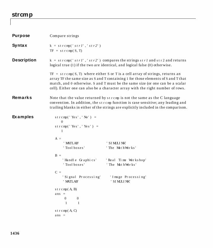
strcmp
1436
1strcmpPurpose Compare strings
Syntax k = strcmp('str1','str2')TF = strcmp(S,T)
Description k = strcmp('str1','str2') compares the strings str1 and str2 and returnslogical true (1) if the two are identical, and logical false (0) otherwise.
TF = strcmp(S,T) where either S or T is a cell array of strings, returns anarray TF the same size as S and T containing 1 for those elements of S and T thatmatch, and 0 otherwise. S and T must be the same size (or one can be a scalarcell). Either one can also be a character array with the right number of rows.
Remarks Note that the value returned by strcmp is not the same as the C languageconvention. In addition, the strcmp function is case sensitive; any leading andtrailing blanks in either of the strings are explicitly included in the comparison.
Examples strcmp('Yes','No') =0
strcmp('Yes','Yes') =1
A ='MATLAB' 'SIMULINK'
'Toolboxes' 'The MathWorks'
B ='Handle Graphics' 'Real Time Workshop'
'Toolboxes' 'The MathWorks'
C ='Signal Processing' 'Image Processing'
'MATLAB' 'SIMULINK'
strcmp(A,B)ans =
0 0 1 1
strcmp(A,C)ans =
strcmp
1437
0 0 0 0
See Also strncmp, strcmpi, strncmpi, strmatch, findstr
strcmpi
1438
1strcmpiPurpose Compare strings ignoring case
Syntax strcmpi(str1,str2)strcmpi(S,T)
Description strcmpi(str1,str2) returns 1 if strings str1 and str2 are the same exceptfor case and 0 otherwise.
strcmpi(S,T) when either S or T is a cell array of strings, returns an array thesame size as S and T containing 1 for those elements of S and T that matchexcept for case, and 0 otherwise. S and T must be the same size (or one can bea scalar cell). Either one can also be a character array with the right numberof rows.
strcmpi supports international character sets.
See Also findstr, strcmp, strmatch, strncmpi
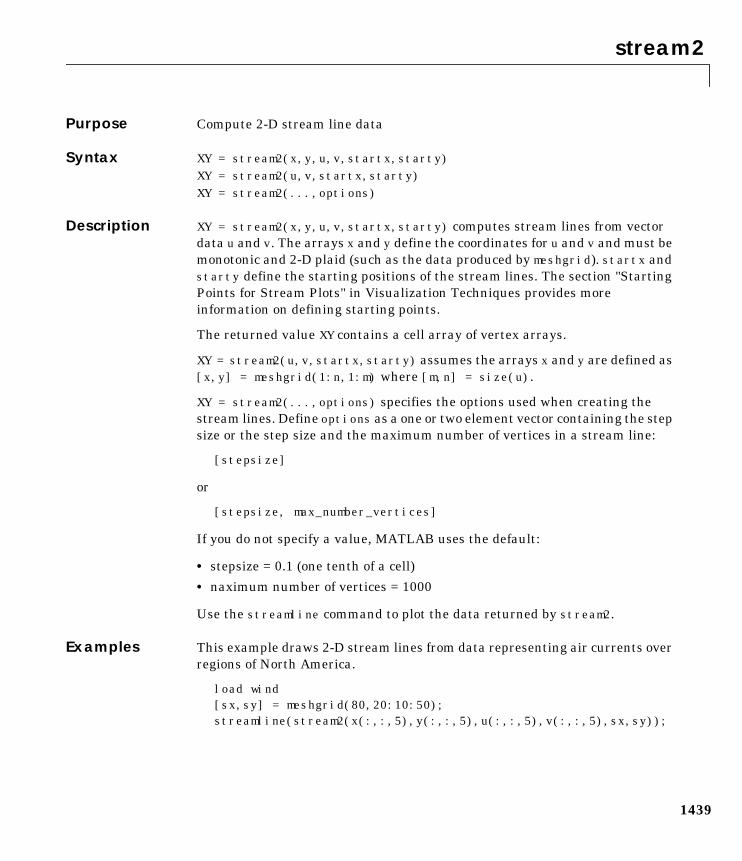
stream2
1439
1stream2Purpose Compute 2-D stream line data
Syntax XY = stream2(x,y,u,v,startx,starty)XY = stream2(u,v,startx,starty)XY = stream2(...,options)
Description XY = stream2(x,y,u,v,startx,starty) computes stream lines from vectordata u and v. The arrays x and y define the coordinates for u and v and must bemonotonic and 2-D plaid (such as the data produced by meshgrid). startx andstarty define the starting positions of the stream lines. The section "StartingPoints for Stream Plots" in Visualization Techniques provides moreinformation on defining starting points.
The returned value XY contains a cell array of vertex arrays.
XY = stream2(u,v,startx,starty) assumes the arrays x and y are defined as[x,y] = meshgrid(1:n,1:m) where [m,n] = size(u).
XY = stream2(...,options) specifies the options used when creating thestream lines. Define options as a one or two element vector containing the stepsize or the step size and the maximum number of vertices in a stream line:
[stepsize]
or
[stepsize, max_number_vertices]
If you do not specify a value, MATLAB uses the default:
• stepsize = 0.1 (one tenth of a cell)
• naximum number of vertices = 1000
Use the streamline command to plot the data returned by stream2.
Examples This example draws 2-D stream lines from data representing air currents overregions of North America.
load wind[sx,sy] = meshgrid(80,20:10:50);streamline(stream2(x(:,:,5),y(:,:,5),u(:,:,5),v(:,:,5),sx,sy));

stream2
1440
See Also coneplot, isosurface, reducevolume smooth3, stream3, streamline,subvolume
stream3
1441
1stream3Purpose Compute 3-D stream line data
Syntax XYZ = stream3(X,Y,Z,U,V,W,startx,starty,startz)XYZ = stream3(U,V,W,startx,starty,startz)
Description XYZ = stream3(X,Y,Z,U,V,W,startx,starty,startz) computes stream linesfrom vector data U, V, W. The arrays X, Y, Z define the coordinates for U, V, W andmust be monotonic and 3-D plaid (such as the data produced by meshgrid).startx, starty, and startz define the starting positions of the stream lines.The section "Starting Points for Stream Plots" in Visualization Techniquesprovides more information on defining starting points.
The returned value XYZ contains a cell array of vertex arrays.
XYZ = stream3(U,V,W,startx,starty,startz) assumes the arrays X, Y, andZ are defined as [X,Y,Z] = meshgrid(1:N,1:M,1:P) where [M,N,P] =size(U).
XYZ = stream3(...,options) specifies the options used when creating thestream lines. Define options as a one or two element vector containing the stepsize or the step size and the maximum number of vertices in a stream line:
[stepsize]
or
[stepsize, max_number_vertices]
If you do not specify values, MATLAB uses the default:
• stepsize = 0.1 (one tenth of a cell)
• naximum number of vertices = 1000
Use the streamline command to plot the data returned by stream3.
Examples This example draws 3-D stream lines from data representing air currents overregions of North America.
load wind[sx sy sz] = meshgrid(80,20:10:50,0:5:15);streamline(stream3(x,y,z,u,v,w,sx,sy,sz))view(3)

stream3
1442
See Also coneplot, isosurface, reducevolume smooth3, stream2, streamline,subvolume
streamline
1443
1streamlinePurpose Draw stream lines from 2-D or 3-D vector data
Syntax h = streamline(X,Y,Z,U,V,W,startx,starty,startz)h = streamline(U,V,W,startx,starty,startz)h = streamline(XYZ)h = streamline(X,Y,U,V,startx,starty)h = streamline(U,V,startx,starty)h = streamline(XY)h = streamline(...,options)
Description h = streamline(X,Y,Z,U,V,W,startx,starty,startz) draws stream linesfrom 3-D vector data U, V, W. The arrays X, Y, Z define the coordinates for U, V, Wand must be monotonic and 3-D plaid (such as the data produced by meshgrid).startx, starty, startz define the starting positions of the stream lines. Thesection "Starting Points for Stream Plots" in Visualization Techniques providesmore information on defining starting points.
The output argument h contains a vector of line handles, one handle for eachstream line.
h = streamline(U,V,W,startx,starty,startz) assumes the arrays X, Y, andZ are defined as [X,Y,Z] = meshgrid(1:N,1:M,1:P) where [M,N,P] =size(U).
h = streamline(XYZ) assumes XYZ is a precomputed cell array of vertex arrays(as produced by stream3).
h = streamline(X,Y,U,V,startx,starty) draws stream lines from 2-D vectordata U, V. The arrays X, Y define the coordinates for U, V and must be monotonicand 2-D plaid (such as the data produced by meshgrid). startx and startydefine the starting positions of the stream lines. The output argument hcontains a vector of line handles, one handle for each stream line.
h = streamline(U,V,startx,starty) assumes the arrays X and Y are definedas [X,Y] = meshgrid(1:N,1:M) where [M,N] = size(U).
h = streamline(XY) assumes XY is a precomputed cell array of vertex arrays(as produced by stream2).
streamline
1444
streamline(...,options) specifies the options used when creating thestream lines. Define options as a one or two element vector containing the stepsize or the step size and the maximum number of vertices in a stream line:
[stepsize]
or
[stepsize, max_number_vertices]
If you do not specify values, MATLAB uses the default:
• stepsize = 0.1 (one tenth of a cell)
• naximum number of vertices = 1000
Examples This example draws stream lines from data representing air currents over aregion of North America. Loading the wind data set creates the variables x, y,z, u, v, and w in the MATLAB workspace.
The plane of stream lines indicates the flow of air from the west to the east (thex direction) beginning at x = 80 (which is close to the minimum value of the xcoordinates). The y and z coordinate starting points are multivalued andapproximately span the range of these coordinates. meshgrid generates thestarting positions of the stream lines.
load wind[sx,sy,sz] = meshgrid(80,20:10:50,0:5:15);h = streamline(x,y,z,u,v,w,sx,sy,sz);set(h,'Color','red')view(3)
See Also stream2, stream3, coneplot, isosurface, smooth3, subvolume, reducevolume
streamparticles
1445
1streamparticlesPurpose Display stream particles
Syntax streamparticles(vertices)streamparticles(vertices,n)streamparticles(...,'PropertyName',PropertyValue,...)streamparticles(line_handle,...)h = streamparticles(...)
Description streamparticles(vertices) draws stream particles of a vector field. Streamparticles are usually represented by markers and can show the position andvelocity of a streamline. vertices is a cell array of 2-D or 3-D vertices (as ifproduced by stream2 or stream3).
streamparticles(vertices,n) uses n to determine how many streamparticles to draw. The ParticleAlignment property controls how n isinterpreted.
• If ParticleAlignment is set to off (the default) and n is greater than 1, thenapproximately n particles are drawn evenly spaced over the streamlinevertices.
If n is less than or equal to 1, n is interpreted as a fraction of the originalstream vertices; for example, if n is 0.2, approximately 20% of the verticesare used.
n determines the upper bound for the number of particles drawn. Note thatthe actual number of particles may deviate from n by as much as a factor of 2.
• If ParticleAlignment is on, n determines the number of particles on thestreamline having the most vertices and sets the spacing on the otherstreamlines to this value. The default value is n = 1.
streamparticles(...,'PropertyName',PropertyValue,...) controls thestream particles using named properties and specified values. Any unspecifiedproperties have default values. MATLAB ignores the case of property names.
Stream Particle PropertiesAnimate – Stream particle motion [non-negative integer]
The number of times to animate the stream particles. The default is 0, whichdoes not animate. Inf animates until you enter ctrl-c.
streamparticles
1446
FrameRate – Animation frames per second [non-negative integer]
This property specifies the number of frames per second for the animation. Inf,the default draws the animation as fast as possible. Note that speed of theanimation may be limited by the speed of the computer. In such cases, thevalue of FrameRate can not necessarily be achieved.
ParticleAlignment – Align particles with stream lines [ on | off ]
Set this property to on to draw particles at the beginning of each the streamline. This property controls how streamparticles interprets the argument n(number of stream particles).
Stream particles are line objects. In addition to stream particle properties, youcan specify any line object property, such as Marker and EraseMode.streamparticles sets the following line properties when called.
You can override any of these properties by specifying a property name andvalue as arguments to streamparticles. For example, this statement usesRGB values to set the MarkerFaceColor to medium gray:
streamparticles(vertices,'MarkerFaceColor',[.5 .5 .5])
streamparticles(line_handle,...) uses the line object identified byline_handle to draw the stream particles.
h = streamparticles(...) returns a vector of handles to the line objects itcreates.
Examples This example combines stream lines with stream particle animation. Theinterpstreamspeed function determines the vertices along the stream lines
Line Property Value Set by streamparticles
EraseMode xor
LineStyle none
Marker o
MarkerEdgeColor none
MarkerFaceColor red
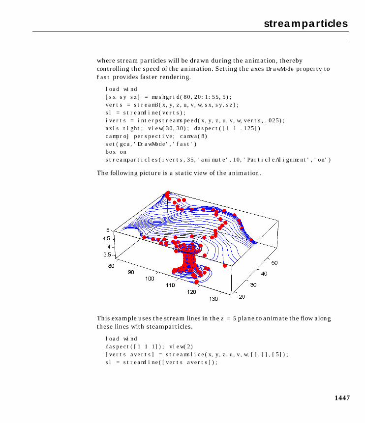
streamparticles
1447
where stream particles will be drawn during the animation, therebycontrolling the speed of the animation. Setting the axes DrawMode property tofast provides faster rendering.
load wind[sx sy sz] = meshgrid(80,20:1:55,5);verts = stream3(x,y,z,u,v,w,sx,sy,sz);sl = streamline(verts);iverts = interpstreamspeed(x,y,z,u,v,w,verts,.025);axis tight; view(30,30); daspect([1 1 .125])camproj perspective; camva(8)set(gca,'DrawMode','fast')box onstreamparticles(iverts,35,'animate',10,'ParticleAlignment','on')
The following picture is a static view of the animation.
This example uses the stream lines in the z = 5 plane to animate the flow alongthese lines with steamparticles.
load winddaspect([1 1 1]); view(2)[verts averts] = streamslice(x,y,z,u,v,w,[],[],[5]);sl = streamline([verts averts]);
streamparticles
1448
axis tight off;set(sl,'Visible','off')iverts = interpstreamspeed(x,y,z,u,v,w,verts,.05);set(gca,'DrawMode','fast','Position',[0 0 1 1],'ZLim',[4.9 5.1])set(gcf,'Color','black')streamparticles(iverts, 200, ... 'Animate',100,'FrameRate',40, ... 'MarkerSize',10,'MarkerFaceColor','yellow')
See Also isosurface, isocaps, smooth3, subvolume, reducevolume, reducepatch,isonormals
streamribbon
1449
1streamribbonPurpose Creates a 3-D stream ribbon plot
Syntax streamribbon(X,Y,Z,U,V,W,startx,starty,startz)streamribbon(U,V,W,startx,starty,startz)streamribbon(vertices,X,Y,Z,cav,speed)streamribbon(vertices,cav,speed)streamribbon(vertices,twistangle)streamribbon(...,width)h = streamribbon(...)
Description streamribbon(X,Y,Z,U,V,W,startx,starty,startz) draws stream ribbonsfrom vector volume data U, V, W. The arrays X, Y, Z define the coordinates for U,V, W and must be monotonic and 3-D plaid (as if produced by meshgrid). startx,starty, and startz define the starting positions of the stream ribbons at thecenter of the ribbons. The section "Starting Points for Stream Plots" inVisualization Techniques provides more information on defining startingpoints.
The twist of the ribbons is proportional to the curl of the vector field. The widthof the ribbons is calculated automatically.
Generally, you should set the DataAspectRatio (daspect) before callingstreamribbon.
streamribbon(U,V,W,startx,starty,startz) assumes X, Y, and Z aredetermined by the expression:
[X,Y,Z] = meshgrid(1:n,1:m,1:p)
where [m,n,p] = size(U).
streamribbon(vertices,X,Y,Z,cav,speed) assumes precomputedstreamline vertices, curl angular velocity, and flow speed. vertices is a cellarray of stream line vertices (as produced by stream3). X, Y, Z, cav, and speedare 3-D arrays.
streamribbon(vertices,cav,speed) assumes X, Y, and Z are determined bythe expression:
[X,Y,Z] = meshgrid(1:n,1:m,1:p)
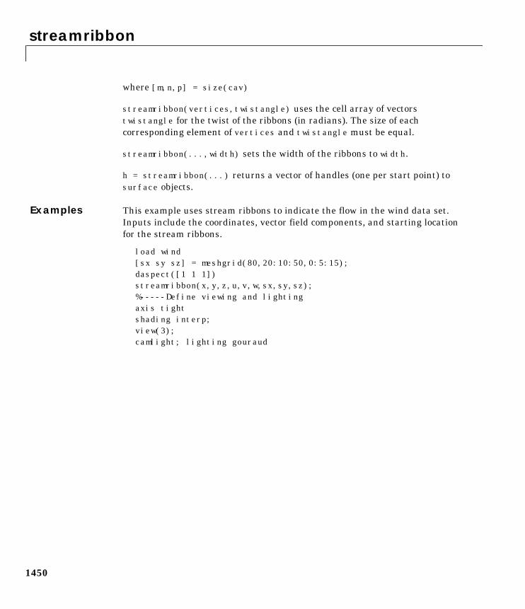
streamribbon
1450
where [m,n,p] = size(cav)
streamribbon(vertices,twistangle) uses the cell array of vectorstwistangle for the twist of the ribbons (in radians). The size of eachcorresponding element of vertices and twistangle must be equal.
streamribbon(...,width) sets the width of the ribbons to width.
h = streamribbon(...) returns a vector of handles (one per start point) tosurface objects.
Examples This example uses stream ribbons to indicate the flow in the wind data set.Inputs include the coordinates, vector field components, and starting locationfor the stream ribbons.
load wind[sx sy sz] = meshgrid(80,20:10:50,0:5:15);daspect([1 1 1])streamribbon(x,y,z,u,v,w,sx,sy,sz);%-----Define viewing and lightingaxis tightshading interp;view(3);camlight; lighting gouraud
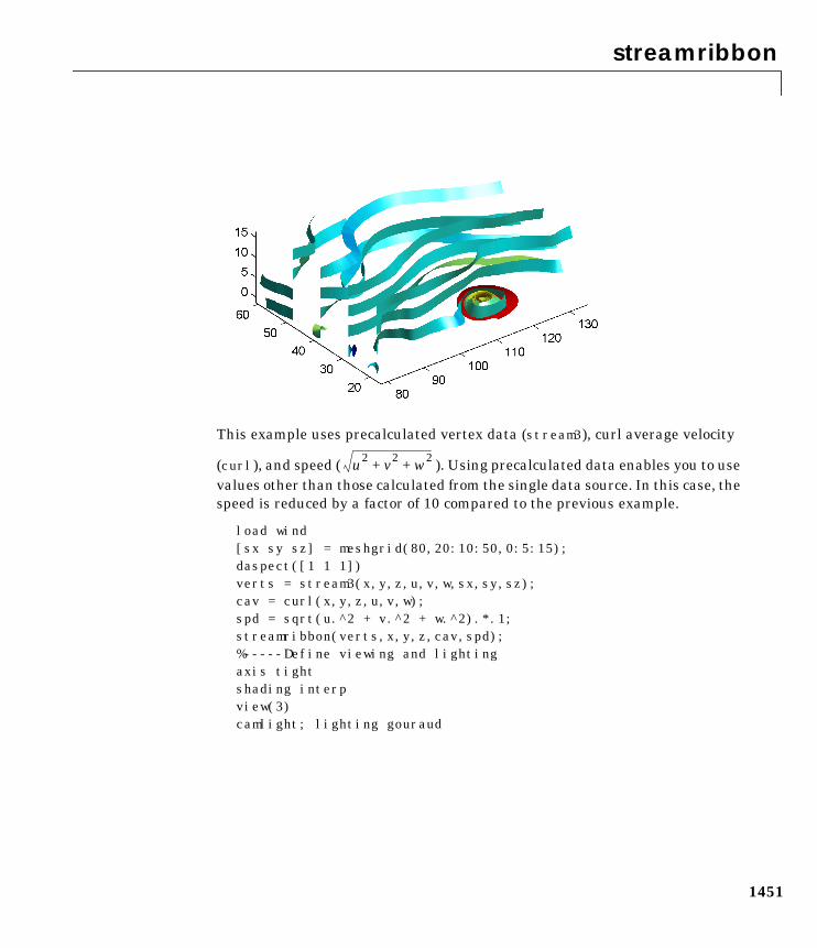
streamribbon
1451
This example uses precalculated vertex data (stream3), curl average velocity
(curl), and speed ( ). Using precalculated data enables you to usevalues other than those calculated from the single data source. In this case, thespeed is reduced by a factor of 10 compared to the previous example.
load wind[sx sy sz] = meshgrid(80,20:10:50,0:5:15);daspect([1 1 1])verts = stream3(x,y,z,u,v,w,sx,sy,sz);cav = curl(x,y,z,u,v,w);spd = sqrt(u.^2 + v.^2 + w.^2).*.1;streamribbon(verts,x,y,z,cav,spd);%-----Define viewing and lightingaxis tightshading interpview(3)camlight; lighting gouraud
u2 v2 w2+ +
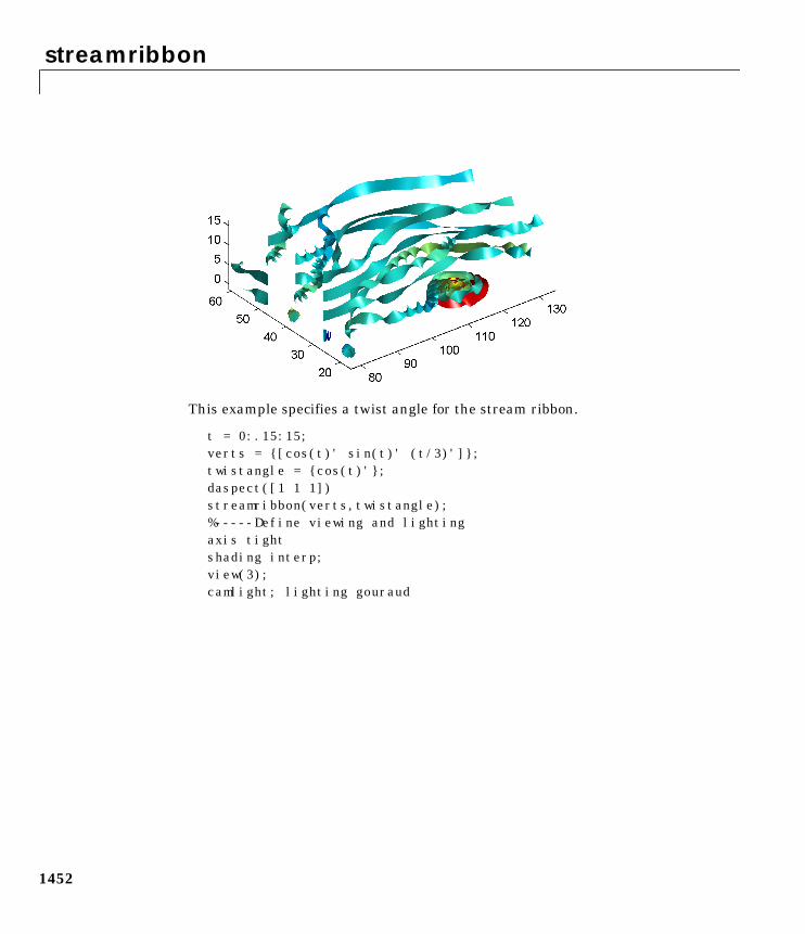
streamribbon
1452
This example specifies a twist angle for the stream ribbon.
t = 0:.15:15;verts = [cos(t)' sin(t)' (t/3)'];twistangle = cos(t)';daspect([1 1 1])streamribbon(verts,twistangle);%-----Define viewing and lightingaxis tightshading interp;view(3);camlight; lighting gouraud
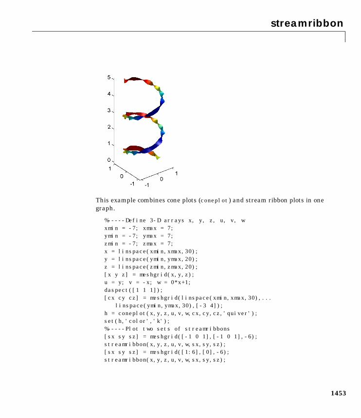
streamribbon
1453
This example combines cone plots (coneplot) and stream ribbon plots in onegraph.
%-----Define 3-D arrays x, y, z, u, v, wxmin = -7; xmax = 7;ymin = -7; ymax = 7;zmin = -7; zmax = 7;x = linspace(xmin,xmax,30);y = linspace(ymin,ymax,20);z = linspace(zmin,zmax,20);[x y z] = meshgrid(x,y,z);u = y; v = -x; w = 0*x+1;daspect([1 1 1]);[cx cy cz] = meshgrid(linspace(xmin,xmax,30),...
linspace(ymin,ymax,30),[-3 4]);h = coneplot(x,y,z,u,v,w,cx,cy,cz,'quiver');set(h,'color','k');%-----Plot two sets of streamribbons[sx sy sz] = meshgrid([-1 0 1],[-1 0 1],-6);streamribbon(x,y,z,u,v,w,sx,sy,sz);[sx sy sz] = meshgrid([1:6],[0],-6);streamribbon(x,y,z,u,v,w,sx,sy,sz);
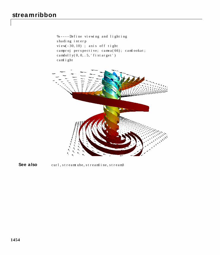
streamribbon
1454
%-----Define viewing and lightingshading interpview(-30,10) ; axis off tightcamproj perspective; camva(66); camlookat;camdolly(0,0,.5,'fixtarget')camlight
See also curl, streamtube, streamline, stream3
streamslice
1455
1streamslicePurpose Draws stream lines in slice planes
Syntax streamslice(X,Y,Z,U,V,W,startx,starty,startz)streamslice(U,V,W,startx,starty,startz)streamslice(X,Y,U,V)streamslice(U,V)streamslice(...,density)streamslice(...,'arrowmode')streamslice(...,'method')h = streamslice(...)[vertices arrowvertices] = streamslice(...)
Description streamslice(X,Y,Z,U,V,W,startx,starty,startz) draws well spacedstreamlines (with direction arrows) from vector data U, V, W in axis aligned x-,y-, z-planes at the points in the vectors startx, starty, startz. (The section"Starting Points for Stream Plots" in Visualization Techniques provides moreinformation on defining starting points.) The arrays X, Y, Z define thecoordinates for U, V, W and must be monotonic and 3-D plaid (as if produced bymeshgrid). U, V, W must be m-by-n-by-p volume arrays.
You should not assumed that the flow is parallel to the slice plane. Forexample, in a stream slice at a constant z, the z component of the vector field,W, is ignored when calculating the streamlines for that plane.
Stream slices are useful for determining where to start stream lines, streamtubes, and stream ribbons.
streamslice(U,V,W,startx,starty,startz) assumes X, Y, and Z aredetermined by the expression:
[X,Y,Z] = meshgrid(1:n,1:m,1:p)
where [m,n,p] = size(U).
streamslice(X,Y,U,V) draws well spaced stream lines (with direction arrows)from vector volume data U, V. The arrays X, Y define the coordinates for U, V andmust be monotonic and 2-D plaid (as if produced by meshgrid).
streamslice(U,V) assumes X, Y, and Z are determined by the expression:
[X,Y,Z] = meshgrid(1:n,1:m,1:p)
streamslice
1456
where [m,n,p] = size(U)
streamslice(...,density) modifies the automatic spacing of the streamlines. density must be greater than 0. The default value is 1; higher valuesproduce more stream lines on each plane. For example, 2 producesapproximately twice as many stream lines, while 0.5 produces approximatelyhalf as many.
streamslice(...,'arrowsmode') determines if direction arrows are presentor not. arrowmode can be:
• arrows – draw direction arrows on the streamlines (default)
• noarrows – does not draw direction arrows
streamslice(...,'method') specifies the interpolation method to use. methodcan be:
• linear – linear interpolation (default)
• cubic – cubic interpolation
• nearest – nearest neighbor interpolation
See interp3 for more information interpolation methods.
h = streamslice(...) returns a vector of handles to the line objects created.
[vertices arrowvertices] = streamslice(...) returns two cell arrays ofvertices for drawing the stream lines and the arrows. You can pass these valuesto any of the stream line drawing functions (streamline, streamribbon,streamtube)
Examples This example creates a stream slice in the wind data set at z = 5.
load winddaspect([1 1 1])streamslice(x,y,z,u,v,w,[],[],[5])axis tight
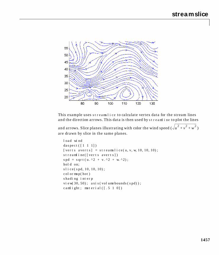
streamslice
1457
This example uses streamslice to calculate vertex data for the stream linesand the direction arrows. This data is then used by streamline to plot the lines
and arrows. Slice planes illustrating with color the wind speed ( )are drawn by slice in the same planes.
load winddaspect([1 1 1])[verts averts] = streamslice(u,v,w,10,10,10);streamline([verts averts])spd = sqrt(u.^2 + v.^2 + w.^2);hold on;slice(spd,10,10,10);colormap(hot)shading interpview(30,50); axis(volumebounds(spd));camlight; material([.5 1 0])
u2 v2 w2+ +
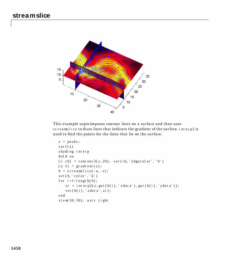
streamslice
1458
This example superimposes contour lines on a surface and then usesstreamslice to draw lines that indicate the gradient of the surface. interp2 isused to find the points for the lines that lie on the surface.
z = peaks;surf(z)shading interphold on[c ch] = contour3(z,20); set(ch,'edgecolor','b')[u v] = gradient(z);h = streamslice(-u,-v);set(h,'color','k')for i=1:length(h);
zi = interp2(z,get(h(i),'xdata'),get(h(i),'ydata'));set(h(i),'zdata',zi);
endview(30,50); axis tight
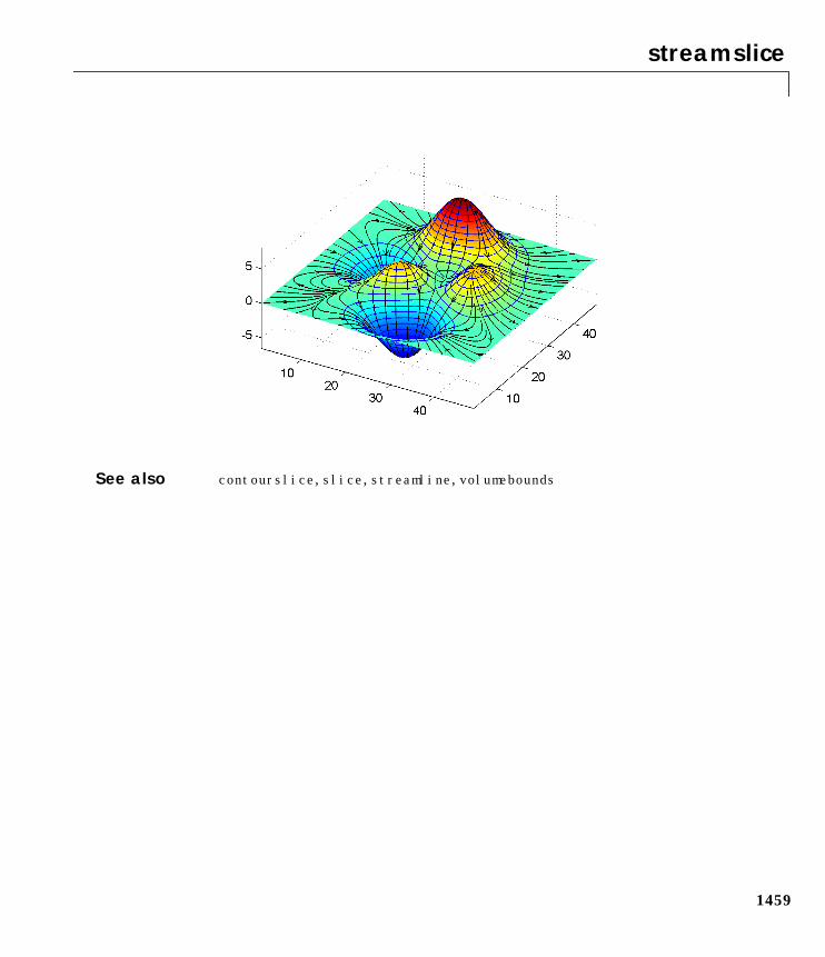
streamslice
1459
See also contourslice, slice, streamline, volumebounds
streamtube
1460
1streamtubePurpose Creates a 3-D stream tube plot
Syntax streamtube(X,Y,Z,U,V,W,startx,starty,startz)streamtube(U,V,W,startx,starty,startz)streamtube(vertices,X,Y,Z,divergence)streamtube(vertices,divergence)streamtube(vertices,width)streamtube(vertices)streamtube(...,[scale n])h = streamtube(...)
Description streamtube(X,Y,Z,U,V,W,startx,starty,startz) draws stream tubes fromvector volume data U, V, W. The arrays X, Y, Z define the coordinates for U, V, Wand must be monotonic and 3-D plaid (as if produced by meshgrid). startx,starty, and startz define the starting positions of the stream lines at thecenter of the tubes. The section "Starting Points for Stream Plots" inVisualization Techniques provides more information on defining startingpoints.
The width of the tubes is proportional to the normalized divergence of thevector field.
Generally, you should set the DataAspectRatio (daspect) before callingstreamtube.
streamtube(U,V,W,startx,starty,startz) assumes X, Y, and Z aredetermined by the expression:
[X,Y,Z] = meshgrid(1:n,1:m,1:p)
where [m,n,p] = size(U).
streamtube(vertices,X,Y,Z,divergence) assumes precomputed stream linevertices and divergence. vertices is a cell array of stream line vertices (asproduced by stream3). X, Y, Z, and divergence are 3-D arrays.
streamtube(vertices,divergence) assumes X, Y, and Z are determined by theexpression:
[X,Y,Z] = meshgrid(1:n,1:m,1:p)
streamtube
1461
where [m,n,p] = size(divergence)
streamtube(vertices,width) specifies the width of the tubes in the cell arrayof vectors, width. The size of each corresponding element of vertices andwidth must be equal. width can also be a scalar, specifying a single value forthe width of all stream tubes.
streamtube(vertices) selects the width automatically.
streamtube(...,[scale n]) scales the width of the tubes by scale. Thedefault is scale = 1. When the stream tubes are created using start points ordivergence, specifying scale = 0 suppresses automatic scaling. n is the numberof points along the circumference of the tube. The default is n = 20.
h = streamtube(...z) returns a vector of handles (one per start point) tosurface objects used to draw the stream tubes.
Examples This example uses stream tubes to indicate the flow in the wind data set.Inputs include the coordinates, vector field components, and starting locationfor the stream tubes.
load wind[sx sy sz] = meshgrid(80,20:10:50,0:5:15);daspect([1 1 1])streamtube(x,y,z,u,v,w,sx,sy,sz);%-----Define viewing and lightingview(3)axis tightshading interp;camlight; lighting gouraud
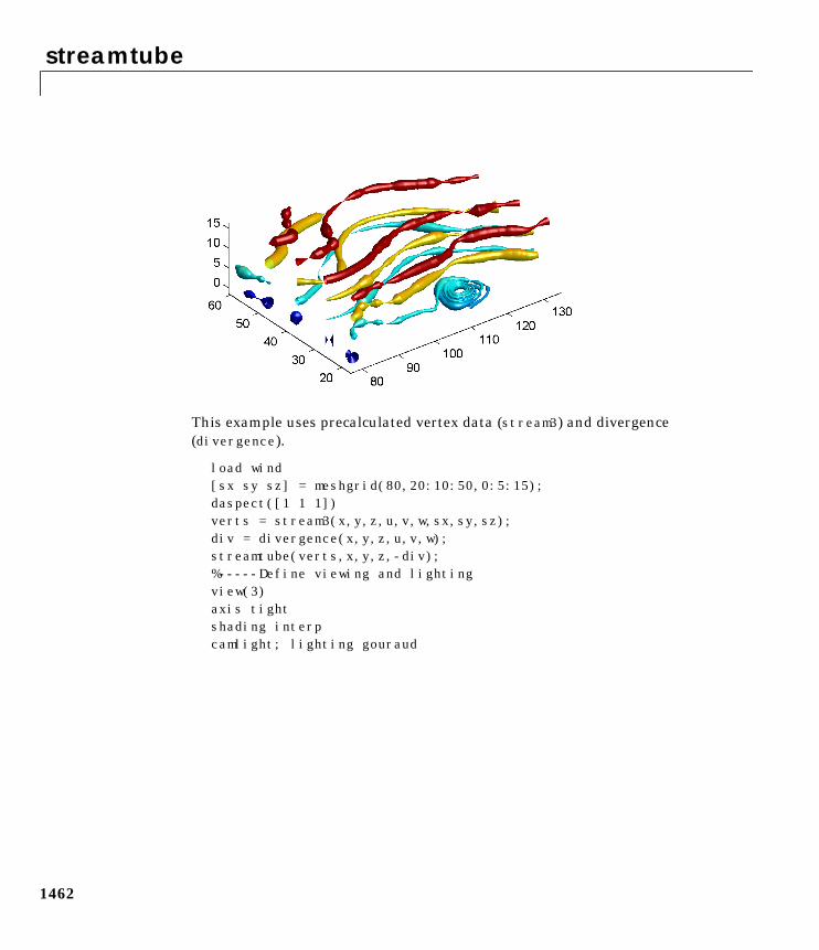
streamtube
1462
This example uses precalculated vertex data (stream3) and divergence(divergence).
load wind[sx sy sz] = meshgrid(80,20:10:50,0:5:15);daspect([1 1 1])verts = stream3(x,y,z,u,v,w,sx,sy,sz);div = divergence(x,y,z,u,v,w);streamtube(verts,x,y,z,-div);%-----Define viewing and lightingview(3)axis tightshading interpcamlight; lighting gouraud
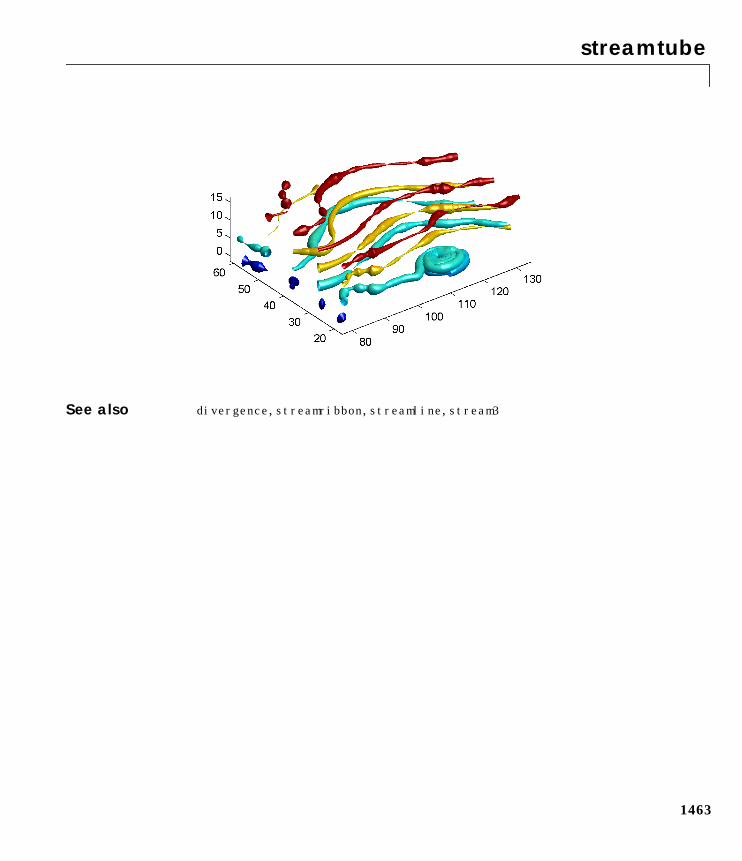
streamtube
1463
See also divergence, streamribbon, streamline, stream3
strings
1464
1stringsPurpose MATLAB string handling
Syntax S = 'Any Characters'S = string(X)X = numeric(S)
Description S = 'Any Characters' is a vector whose components are the numeric codes forthe characters (the first 127 codes are ASCII). The actual characters displayeddepend on the character set encoding for a given font. The length of S is thenumber of characters. A quote within the string is indicated by two quotes.
S = string(X) can be used to convert an array that contains positive integersrepresenting numeric codes into a MATLAB character array.
X = double(S) converts the string to its equivalent numeric codes.
ischar(S) tells if S is a string variable.
Use the strcat function for concatenating cell arrays of strings, for arrays ofmultiple strings, and for padded character arrays. For concatenating two singlestrings, it is more efficient to use square brackets, as shown in the example,than to use strcat.
Examples s = ['It is 1 o''clock', 7]
See Also char, strcat
strjust
1465
1strjustPurpose Justify a character array
Syntax T = strjust(S)T = strjust(S,'right')T = strjust(S,'left')T = strjust(S,'center')
Description T = strjust(S) or T = strjust(S,'right') returns a right-justified versionof the character array S.
T = strjust(S,'left') returns a left-justified version of S.
T = strjust(S,'center') returns a center-justified version of S.
See Also deblank
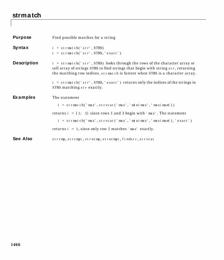
strmatch
1466
1strmatchPurpose Find possible matches for a string
Syntax i = strmatch('str',STRS)i = strmatch('str',STRS,'exact')
Description i = strmatch('str',STRS) looks through the rows of the character array orcell array of strings STRS to find strings that begin with string str, returningthe matching row indices. strmatch is fastest when STRS is a character array.
i = strmatch('str',STRS,'exact') returns only the indices of the strings inSTRS matching str exactly.
Examples The statement
i = strmatch('max',strvcat('max','minimax','maximum'))
returns i = [1; 3] since rows 1 and 3 begin with 'max'. The statement
i = strmatch('max',strvcat('max','minimax','maximum'),'exact')
returns i = 1, since only row 1 matches 'max' exactly.
See Also strcmp, strcmpi, strncmp, strncmpi, findstr, strvcat
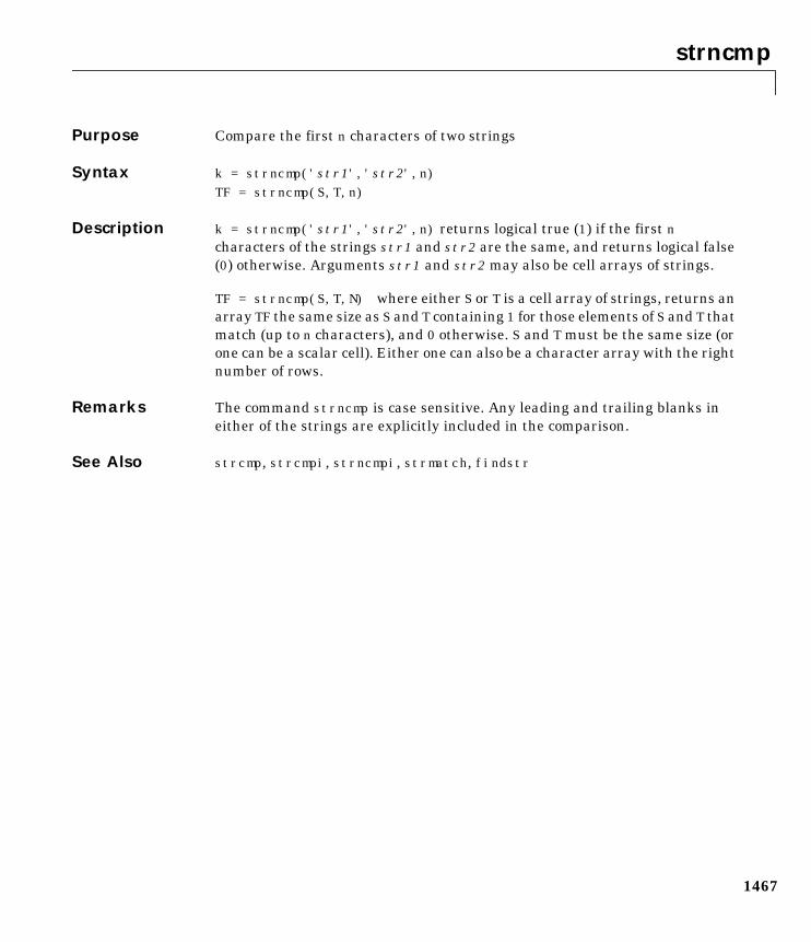
strncmp
1467
1strncmpPurpose Compare the first n characters of two strings
Syntax k = strncmp('str1','str2',n)TF = strncmp(S,T,n)
Description k = strncmp('str1','str2',n) returns logical true (1) if the first ncharacters of the strings str1 and str2 are the same, and returns logical false(0) otherwise. Arguments str1 and str2 may also be cell arrays of strings.
TF = strncmp(S,T,N) where either S or T is a cell array of strings, returns anarray TF the same size as S and T containing 1 for those elements of S and T thatmatch (up to n characters), and 0 otherwise. S and T must be the same size (orone can be a scalar cell). Either one can also be a character array with the rightnumber of rows.
Remarks The command strncmp is case sensitive. Any leading and trailing blanks ineither of the strings are explicitly included in the comparison.
See Also strcmp, strcmpi, strncmpi, strmatch, findstr
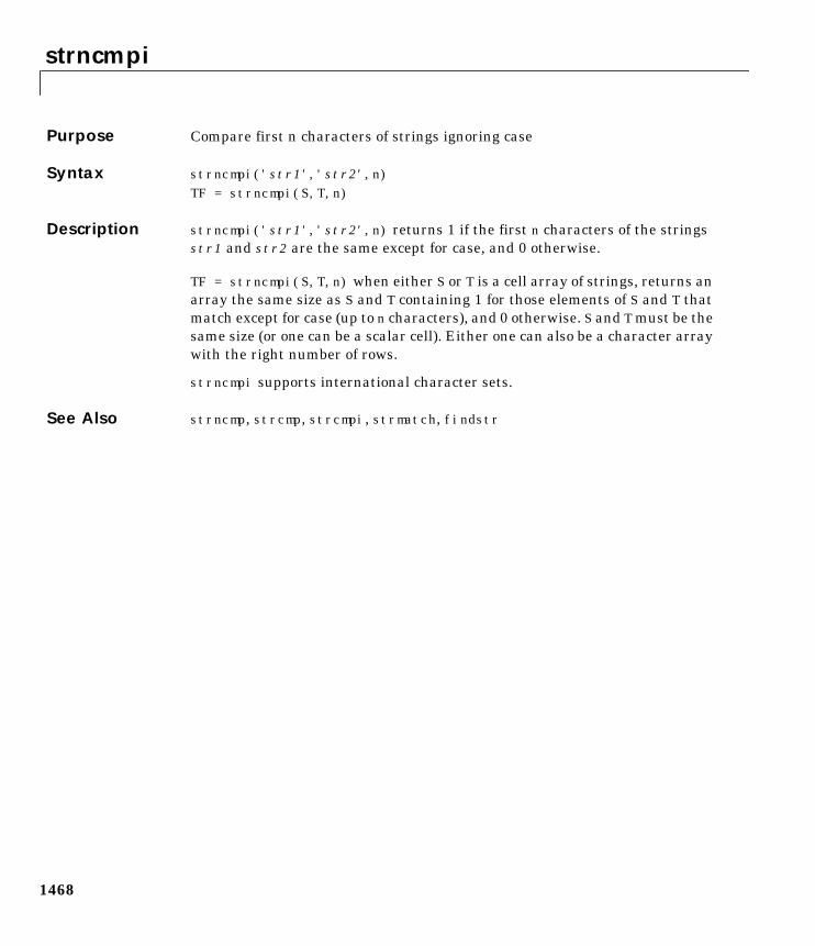
strncmpi
1468
1strncmpiPurpose Compare first n characters of strings ignoring case
Syntax strncmpi('str1','str2',n)TF = strncmpi(S,T,n)
Description strncmpi('str1','str2',n) returns 1 if the first n characters of the stringsstr1 and str2 are the same except for case, and 0 otherwise.
TF = strncmpi(S,T,n) when either S or T is a cell array of strings, returns anarray the same size as S and T containing 1 for those elements of S and T thatmatch except for case (up to n characters), and 0 otherwise. S and T must be thesame size (or one can be a scalar cell). Either one can also be a character arraywith the right number of rows.
strncmpi supports international character sets.
See Also strncmp, strcmp, strcmpi, strmatch, findstr
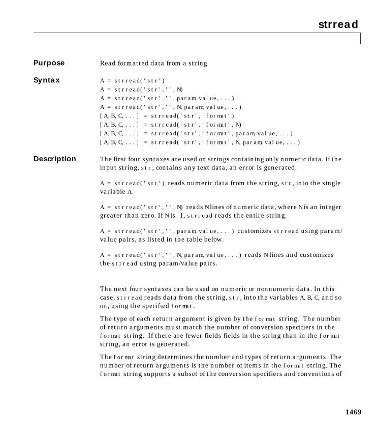
strread
1469
1strreadPurpose Read formatted data from a string
Syntax A = strread('str')A = strread('str','',N)A = strread('str','',param,value,...)A = strread('str','',N,param,value,...)[A,B,C,...] = strread('str','format')[A,B,C,...] = strread('str','format',N)[A,B,C,...] = strread('str','format',param,value,...)[A,B,C,...] = strread('str','format',N,param,value,...)
Description The first four syntaxes are used on strings containing only numeric data. If theinput string, str, contains any text data, an error is generated.
A = strread('str') reads numeric data from the string, str, into the singlevariable A.
A = strread('str','',N) reads N lines of numeric data, where N is an integergreater than zero. If N is -1, strread reads the entire string.
A = strread('str','',param,value,...) customizes strread using param/value pairs, as listed in the table below.
A = strread('str','',N,param,value,...) reads N lines and customizesthe strread using param/value pairs.
The next four syntaxes can be used on numeric or nonnumeric data. In thiscase, strread reads data from the string, str, into the variables A, B, C, and soon, using the specified format.
The type of each return argument is given by the format string. The numberof return arguments must match the number of conversion specifiers in theformat string. If there are fewer fields fields in the string than in the formatstring, an error is generated.
The format string determines the number and types of return arguments. Thenumber of return arguments is the number of items in the format string. Theformat string supports a subset of the conversion specifiers and conventions of
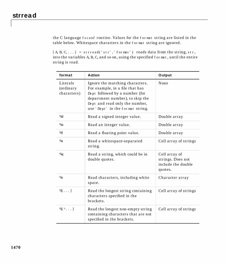
strread
1470
the C language fscanf routine. Values for the format string are listed in thetable below. Whitespace characters in the format string are ignored.
[A,B,C,...] = strread('str','format') reads data from the string, str,into the variables A, B, C, and so on, using the specified format, until the entirestring is read.
format Action Output
Literals(ordinarycharacters)
Ignore the matching characters.For example, in a file that hasDept followed by a number (fordepartment number), to skip theDept and read only the number,use 'Dept' in the format string.
None
%d Read a signed integer value. Double array
%u Read an integer value. Double array
%f Read a floating point value. Double array
%s Read a whitespace-separatedstring.
Cell array of strings
%q Read a string, which could be indouble quotes.
Cell array ofstrings. Does notinclude the doublequotes.
%c Read characters, including whitespace.
Character array
%[...] Read the longest string containingcharacters specified in thebrackets.
Cell array of strings
%[^...] Read the longest non-empty stringcontaining characters that are notspecified in the brackets.
Cell array of strings
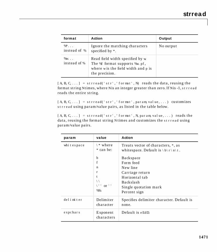
strread
1471
[A,B,C,...] = strread('str','format',N) reads the data, reusing theformat string N times, where N is an integer greater than zero. If N is -1, strreadreads the entire string.
[A,B,C,...] = strread('str','format',param,value,...) customizesstrread using param/value pairs, as listed in the table below.
[A,B,C,...] = strread('str','format',N,param,value,...) reads thedata, reusing the format string N times and customizes the strread usingparam/value pairs.
%*...instead of %
Ignore the matching charactersspecified by *.
No output
%w...instead of %
Read field width specified by w.The %f format supports %w.pf,where w is the field width and p isthe precision.
param value Action
whitespace \* where* can be:
Treats vector of characters, *, aswhitespace. Default is \b\r\n\t.
bfnrt\\\'' or ''%%
BackspaceForm feedNew lineCarriage returnHorizontal tabBackslashSingle quotation markPercent sign
delimiter Delimitercharacter
Specifies delimiter character. Default isnone.
expchars Exponentcharacters
Default is eEdD.
format Action Output
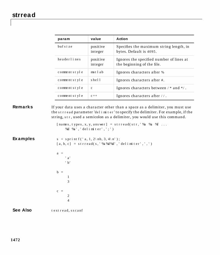
strread
1472
Remarks If your data uses a character other than a space as a delimiter, you must usethe strread parameter 'delimiter' to specify the delimiter. For example, if thestring, str, used a semicolon as a delimiter, you would use this command.
[names,types,x,y,answer] = strread(str,'%s %s %f ... %d %s','delimiter',';')
Examples s = sprintf('a,1,2\nb,3,4\n');[a,b,c] = strread(s,'%s%d%d','delimiter',',')
a = 'a' 'b'
b = 1 3
c = 2 4
See Also textread, sscanf
bufsize positiveinteger
Specifies the maximum string length, inbytes. Default is 4095.
headerlines positiveinteger
Ignores the specified number of lines atthe beginning of the file.
commentstyle matlab Ignores characters after %
commentstyle shell Ignores characters after #.
commentstyle c Ignores characters between /* and */.
commentstyle c++ Ignores characters after //.
param value Action
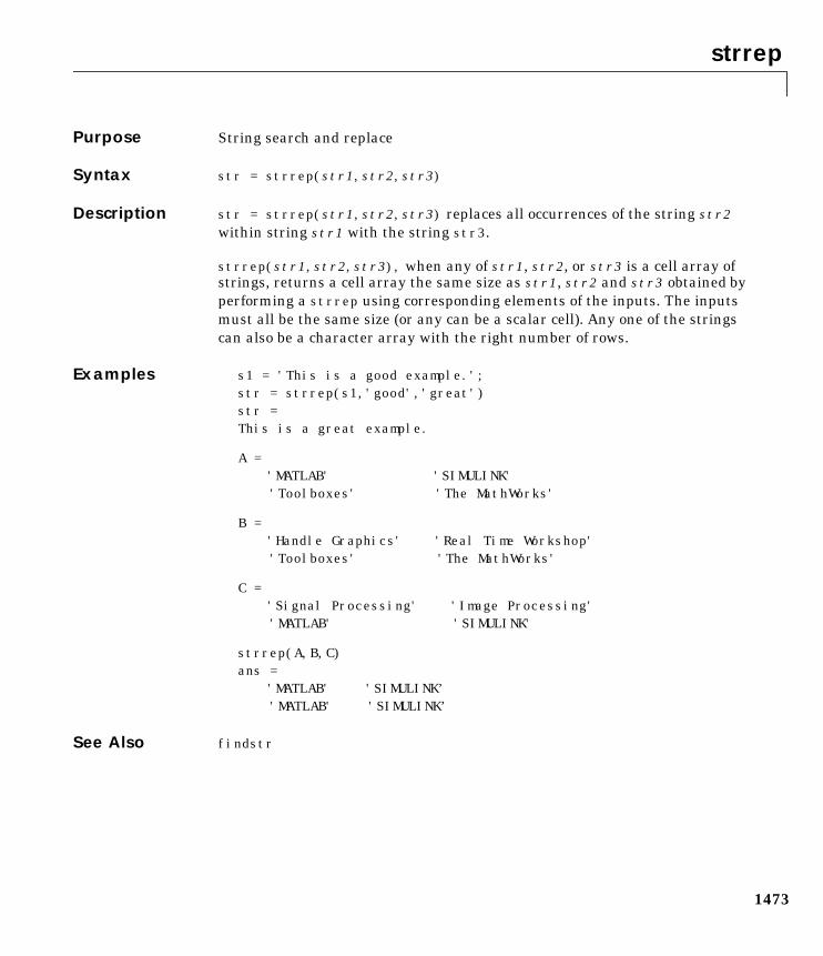
strrep
1473
1strrepPurpose String search and replace
Syntax str = strrep(str1,str2,str3)
Description str = strrep(str1,str2,str3) replaces all occurrences of the string str2within string str1 with the string str3.
strrep(str1,str2,str3), when any of str1, str2, or str3 is a cell array ofstrings, returns a cell array the same size as str1, str2 and str3 obtained byperforming a strrep using corresponding elements of the inputs. The inputsmust all be the same size (or any can be a scalar cell). Any one of the stringscan also be a character array with the right number of rows.
Examples s1 = 'This is a good example.';str = strrep(s1,'good','great')str =This is a great example.
A ='MATLAB' 'SIMULINK'
'Toolboxes' 'The MathWorks'
B ='Handle Graphics' 'Real Time Workshop'
'Toolboxes' 'The MathWorks'
C ='Signal Processing' 'Image Processing'
'MATLAB' 'SIMULINK'
strrep(A,B,C)ans =
'MATLAB' 'SIMULINK’ 'MATLAB' 'SIMULINK’
See Also findstr
strtok
1474
1strtokPurpose First token in string
Syntax token = strtok('str',delimiter)token = strtok('str')[token,rem] = strtok(...)
Description token = strtok('str',delimiter) returns the first token in the text stringstr, that is, the first set of characters before a delimiter is encountered. Thevector delimiter contains valid delimiter characters. Any leading delimitersare ignored.
token = strtok('str') uses the default delimiters, the white spacecharacters. These include tabs (ASCII 9), carriage returns (ASCII 13), andspaces (ASCII 32). Any leading white space characters are ignored.
[token,rem] = strtok(...) returns the remainder rem of the original string.The remainder consists of all characters from the first delimiter on.
Examples s = ' This is a good example.';[token,rem] = strtok(s)token =Thisrem =is a good example.
See Also findstr, strmatch
struct
1475
1structPurpose Create structure array
Syntax s = struct('field1',,'field2',,...)s = struct('field1',values1,'field2',values2,...)
Description s = struct('field1',,'field2',,...) creates an empty structure withfields field1, field2, ...
s = struct('field1',values1,'field2',values2,...) creates a structurearray with the specified fields and values. The value arrays values1, values2,etc. must be cell arrays of the same size or scalar cells. Corresponding elementsof the value arrays are placed into corresponding structure array elements. Thesize of the resulting structure is the same size as the value cell arrays or 1-by-1if none of the values is a cell.
Examples The command
s = struct('type','big','little','color','red','x',3 4)
produces a structure array s:
s =1x2 struct array with fields: type color x
The value arrays have been distributed among the fields of s:
s(1)ans =
type: 'big' color: 'red' x: 3
s(2)ans =
type: 'little' color: 'red' x: 4
struct
1476
Similarly, the command
a.b = struct('z',);
produces an empty structure a.b with field z.
a.bans = 0x0 struct array with fields: z
See Also fieldnames, getfield, rmfield, setfield
struct2cell
1477
1struct2cellPurpose Structure to cell array conversion
Syntax c = struct2cell(s)
Description c = struct2cell(s) converts the m-by-n structure s (with p fields) into ap-by-m-by-n cell array c.
If structure s is multidimensional, cell array c has size [p size(s)].
Examples The commands
clear s, s.category = 'tree';s.height = 37.4; s.name = 'birch';
create the structure
s = category: 'tree' height: 37.4000 name: 'birch'
Converting the structure to a cell array,
c = struct2cell(s)
c = 'tree' [37.4000] 'birch'
See Also cell2struct, fieldnames
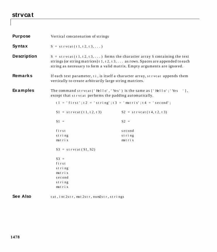
strvcat
1478
1strvcatPurpose Vertical concatenation of strings
Syntax S = strvcat(t1,t2,t3,...)
Description S = strvcat(t1,t2,t3,...) forms the character array S containing the textstrings (or string matrices) t1,t2,t3,... as rows. Spaces are appended to eachstring as necessary to form a valid matrix. Empty arguments are ignored.
Remarks If each text parameter, ti, is itself a character array, strvcat appends themvertically to create arbitrarily large string matrices.
Examples The command strvcat('Hello','Yes') is the same as ['Hello';'Yes '],except that strvcat performs the padding automatically.
t1 = 'first';t2 = 'string';t3 = 'matrix';t4 = 'second';
S1 = strvcat(t1,t2,t3) S2 = strvcat(t4,t2,t3)
S1 = S2 =
first secondstring stringmatrix matrix
S3 = strvcat(S1,S2)
S3 =firststringmatrixsecondstringmatrix
See Also cat, int2str, mat2str, num2str, strings
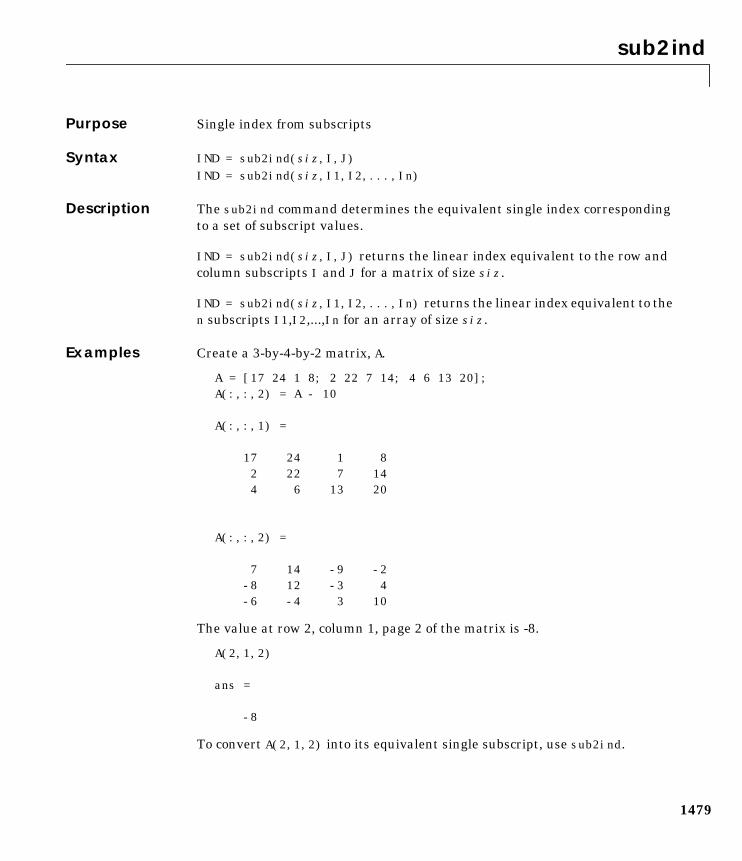
sub2ind
1479
1sub2indPurpose Single index from subscripts
Syntax IND = sub2ind(siz,I,J)IND = sub2ind(siz,I1,I2,...,In)
Description The sub2ind command determines the equivalent single index correspondingto a set of subscript values.
IND = sub2ind(siz,I,J) returns the linear index equivalent to the row andcolumn subscripts I and J for a matrix of size siz.
IND = sub2ind(siz,I1,I2,...,In) returns the linear index equivalent to then subscripts I1,I2,...,In for an array of size siz.
Examples Create a 3-by-4-by-2 matrix, A.
A = [17 24 1 8; 2 22 7 14; 4 6 13 20];A(:,:,2) = A - 10
A(:,:,1) =
17 24 1 8 2 22 7 14 4 6 13 20
A(:,:,2) =
7 14 -9 -2 -8 12 -3 4 -6 -4 3 10
The value at row 2, column 1, page 2 of the matrix is -8.
A(2,1,2)
ans =
-8
To convert A(2,1,2) into its equivalent single subscript, use sub2ind.
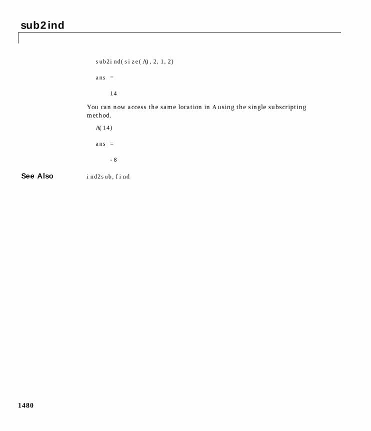
sub2ind
1480
sub2ind(size(A),2,1,2)
ans =
14
You can now access the same location in A using the single subscriptingmethod.
A(14)
ans =
-8
See Also ind2sub, find
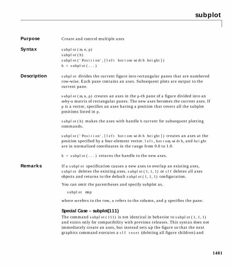
subplot
1481
1subplotPurpose Create and control multiple axes
Syntax subplot(m,n,p)subplot(h)subplot('Position',[left bottom width height])h = subplot(...)
Description subplot divides the current figure into rectangular panes that are numberedrow-wise. Each pane contains an axes. Subsequent plots are output to thecurrent pane.
subplot(m,n,p) creates an axes in the p-th pane of a figure divided into anm-by-n matrix of rectangular panes. The new axes becomes the current axes. Ifp is a vector, specifies an axes having a position that covers all the subplotpositions listed in p.
subplot(h) makes the axes with handle h current for subsequent plottingcommands.
subplot('Position',[left bottom width height]) creates an axes at theposition specified by a four-element vector. left, bottom, width, and heightare in normalized coordinates in the range from 0.0 to 1.0.
h = subplot(...) returns the handle to the new axes.
Remarks If a subplot specification causes a new axes to overlap an existing axes,subplot deletes the existing axes. subplot(1,1,1) or clf deletes all axesobjects and returns to the default subplot(1,1,1) configuration.
You can omit the parentheses and specify subplot as.
subplot mnp
where m refers to the row, n refers to the column, and p specifies the pane.
Special Case – subplot(111)The command subplot(111) is not identical in behavior to subplot(1,1,1)and exists only for compatibility with previous releases. This syntax does notimmediately create an axes, but instead sets up the figure so that the nextgraphics command executes a clf reset (deleting all figure children) and
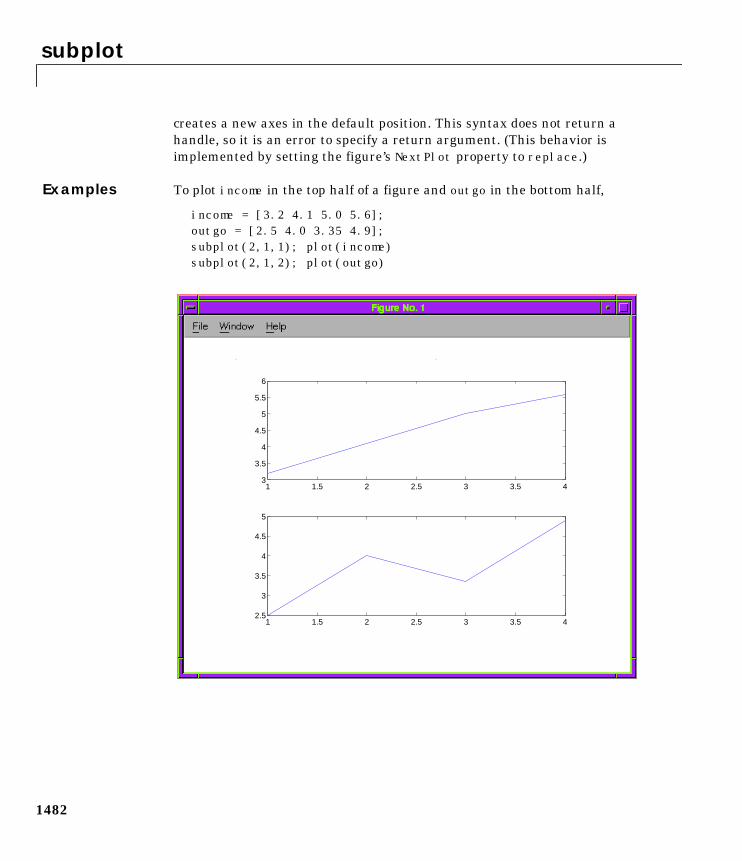
subplot
1482
creates a new axes in the default position. This syntax does not return ahandle, so it is an error to specify a return argument. (This behavior isimplemented by setting the figure’s NextPlot property to replace.)
Examples To plot income in the top half of a figure and outgo in the bottom half,
income = [3.2 4.1 5.0 5.6];outgo = [2.5 4.0 3.35 4.9];subplot(2,1,1); plot(income)subplot(2,1,2); plot(outgo)
1 1.5 2 2.5 3 3.5 43
3.5
4
4.5
5
5.5
6
1 1.5 2 2.5 3 3.5 42.5
3
3.5
4
4.5
5
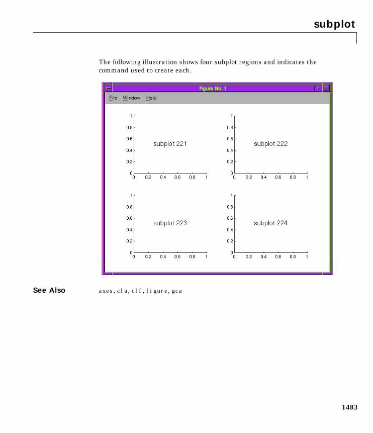
subplot
1483
The following illustration shows four subplot regions and indicates thecommand used to create each.
See Also axes, cla, clf, figure, gca
subsasgn
1484
1subsasgnPurpose Overloaded method for A(I)=B, AI=B, and A.field=B
Syntax A = subsasgn(A,S,B)
Description A = subsasgn(A,S,B) is called for the syntax A(i)=B, Ai=B, or A.i=B whenA is an object. S is a structure array with the fields:
• type: A string containing '()', '', or '.', where '()' specifies integersubscripts; '' specifies cell array subscripts, and '.' specifies subscriptedstructure fields.
• subs: A cell array or string containing the actual subscripts.
Remarks subsasgn is designed to be used by the MATLAB interpreter to handleindexedassignments to objects. Calling subsasgn directly as a function is notrecommended. If you do use subsasgn in this way, it conforms to the formalMATLAB dispatching rules and may yield unexpected results.
Examples The syntax A(1:2,:)=B calls A=subsasgn(A,S,B) where S is a 1-by-1 structurewith S.type='()' and S.subs = 1:2,':'. A colon used as a subscript ispassed as the string ':'.
The syntax A1:2=B calls A=subsasgn(A,S,B) where S.type='' .
The syntax A.field=B calls subsasgn(A,S,B) where S.type='.' andS.subs='field'.
These simple calls are combined in a straightforward way for more complicatedsubscripting expressions. In such cases length(S) is the number ofsubscripting levels. For instance, A(1,2).name(3:5)=B callsA=subsasgn(A,S,B) where S is 3-by-1 structure array with the followingvalues:
See Also subsref
See “Handling Subscripted Assignment” for more information aboutoverloaded methods and subsasgn.
S(1).type='()' S(2).type='.' S(3).type='()'
S(1).subs=1,2 S(2).subs='name' S(3).subs=3:5
subsindex
1485
1subsindexPurpose Overloaded method for X(A)
Syntax i = subsindex(A)
Description i = subsindex(A) is called for the syntax 'X(A)' when A is an object.subsindex must return the value of the object as a zero-based integer index (imust contain integer values in the range 0 to prod(size(X))-1). subsindex iscalled by the default subsref and subsasgn functions, and you can call it if youoverload these functions.
See Also subsasgn, subsref
subspace
1486
1subspacePurpose Angle between two subspaces
Syntax theta = subspace(A,B)
Description theta = subspace(A,B) finds the angle between two subspaces specified bythe columns of A and B. If A and B are column vectors of unit length, this is thesame as acos(A'∗B).
Remarks If the angle between the two subspaces is small, the two spaces are nearlylinearly dependent. In a physical experiment described by some observationsA, and a second realization of the experiment described by B, subspace(A,B)gives a measure of the amount of new information afforded by the secondexperiment not associated with statistical errors of fluctuations.
Examples Consider two subspaces of a Hadamard matrix, whose columns are orthogonal.
H = hadamard(8);A = H(:,2:4);B = H(:,5:8);
Note that matrices A and B are different sizes— A has three columns and B four.It is not necessary that two subspaces be the same size in order to find theangle between them. Geometrically, this is the angle between two hyperplanesembedded in a higher dimensional space.
theta = subspace(A,B)theta = 1.5708
That A and B are orthogonal is shown by the fact that theta is equal to π/2.
theta - pi/2ans = 0
subsref
1487
1subsrefPurpose Overloaded method for A(I), AI and A.field
Syntax B = subsref(A,S)
Description B = subsref(A,S) is called for the syntax A(i), Ai, or A.i when A is anobject. S is a structure array with the fields:
• type: A string containing '()', '', or '.', where '()' specifies integersubscripts; '' specifies cell array subscripts, and '.' specifies subscriptedstructure fields.
• subs: A cell array or string containing the actual subscripts.
Remarks subsref is designed to be used by the MATLAB interpreter to handleindexedreferences to objects. Calling subsref directly as a function is notrecommended. If you do use subsref in this way, it conforms to the formalMATLAB dispatching rules and may yield unexpected results.
Examples The syntax A(1:2,:) calls subsref(A,S) where S is a 1-by-1 structure withS.type='()' and S.subs=1:2,':'. A colon used as a subscript is passed asthe string ':'.
The syntax A1:2 calls subsref(A,S) where S.type='' and S.subs=1:2.
The syntax A.field calls subsref(A,S) where S.type='.' andS.subs='field'.
These simple calls are combined in a straightforward way for more complicatedsubscripting expressions. In such cases length(S) is the number ofsubscripting levels. For instance, A(1,2).name(3:5) calls subsref(A,S)whereS is 3-by-1 structure array with the following values:
See Also subsasgn
See “Handling Subscripted Reference” for more information about overloadedmethods and subsref.
S(1).type='()' S(2).type='.' S(3).type='()'
S(1).subs=1,2 S(2).subs='name' S(3).subs=3:5
subvolume
1488
1 subvolumePurpose Extract subset of volume data set
Syntax [Nx,Ny,Nz,Nv] = subvolume(X,Y,Z,V,limits)[Nx,Ny,Nz,Nv] = subvolume(V,limits)Nv = subvolume(...)
Description [Nx,Ny,Nz,Nv] = subvolume(X,Y,Z,V,limits) extracts a subset of thevolume data set V using the specified axis-aligned limits. limits =[xmin,xmax,ymin, ymax,zmin,zmax] (Any NaNs in the limits indicate that thevolume should not be cropped along that axis).
The arrays X, Y, and Z define the coordinates for the volume V. The subvolumeis returned in NV and the coordinates of the subvolume are given in NX, NY, andNZ.
[Nx,Ny,Nz,Nv] = subvolume(V,limits) assumes the arrays X, Y, and Z aredefined as [X,Y,Z] = meshgrid(1:N,1:M,1:P) where [M,N,P] = size(V).
Nv = subvolume(...) returns only the subvolume.
Examples This example uses a data set that is a collection of MRI slices of a human skull.The data is processed in a variety of ways:
• The 4-D array is squeezed (squeeze) into three dimensions and then a subsetof the data is extracted (subvolume).
• The outline of the skull is an isosurface generated as a patch (p1) whosevertex normals are recalculated to improve the appearance when lighting isapplied (patch, isosurface, isonormals).
• A second patch (p2) with interpolated face color draws the end caps(FaceColor, isocaps).
• The view of the object is set (view, axis, daspect).
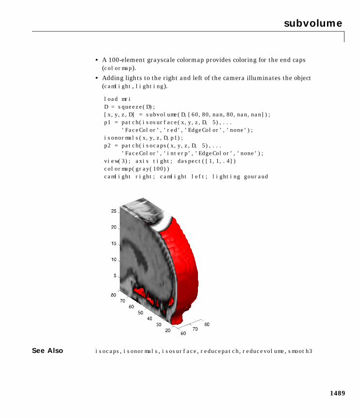
subvolume
1489
• A 100-element grayscale colormap provides coloring for the end caps(colormap).
• Adding lights to the right and left of the camera illuminates the object(camlight, lighting).
load mriD = squeeze(D);[x,y,z,D] = subvolume(D,[60,80,nan,80,nan,nan]);p1 = patch(isosurface(x,y,z,D, 5),...
’FaceColor’,’red’,’EdgeColor’,’none’);isonormals(x,y,z,D,p1);p2 = patch(isocaps(x,y,z,D, 5),...
’FaceColor’,’interp’,’EdgeColor’,’none’);view(3); axis tight; daspect([1,1,.4])colormap(gray(100))camlight right; camlight left; lighting gouraud
See Also isocaps, isonormals, isosurface, reducepatch, reducevolume, smooth3
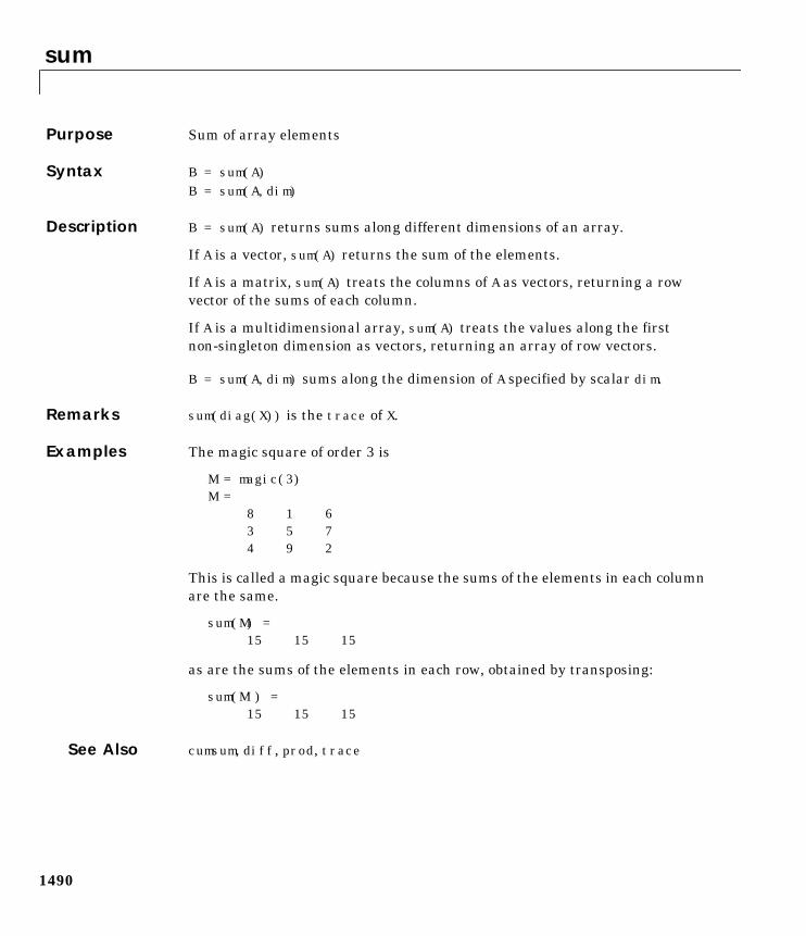
sum
1490
1 sumPurpose Sum of array elements
Syntax B = sum(A)B = sum(A,dim)
Description B = sum(A) returns sums along different dimensions of an array.
If A is a vector, sum(A) returns the sum of the elements.
If A is a matrix, sum(A) treats the columns of A as vectors, returning a rowvector of the sums of each column.
If A is a multidimensional array, sum(A) treats the values along the firstnon-singleton dimension as vectors, returning an array of row vectors.
B = sum(A,dim) sums along the dimension of A specified by scalar dim.
Remarks sum(diag(X)) is the trace of X.
Examples The magic square of order 3 is
M = magic(3)M =
8 1 63 5 74 9 2
This is called a magic square because the sums of the elements in each columnare the same.
sum(M) =15 15 15
as are the sums of the elements in each row, obtained by transposing:
sum(M') =15 15 15
See Also cumsum, diff, prod, trace
superiorto
1491
1superiortoPurpose Superior class relationship
Syntax superiorto('class1','class2',...)
Description The superiorto function establishes a hierarchy that determines the order inwhich MATLAB calls object methods.
superiorto('class1','class2',...) invoked within a class constructormethod (say myclass.m) indicates that myclass's method should be invoked ifa function is called with an object of class myclass and one or more objects ofclass class1, class2, and so on.
Remarks Suppose A is of class 'class_a', B is of class 'class_b' and C is of class'class_c'. Also suppose the constructor class_c.m contains the statement:superiorto('class_a'). Then e = fun(a,c) or e = fun(c,a) invokesclass_c/fun.
If a function is called with two objects having an unspecified relationship, thetwo objects are considered to have equal precedence, and the leftmost object’smethod is called. So, fun(b,c) calls class_b/fun, while fun(c,b) callsclass_c/fun.
See Also inferiorto
support
1492
1supportPurpose Open MathWorks Technical Support Web Page
Syntax support
Description support opens your web browser to The MathWorks Technical Support WebPage at http://www.mathworks.com/support.
This page contains the following items:
• A Solution Search Engine
• The "Virtual Technical Support Engineer" that, through a series ofquestions, determines possible solutions to the problems you areexperiencing
• Technical Notes
• Tutorials
• Bug fixes and patches
See Also web
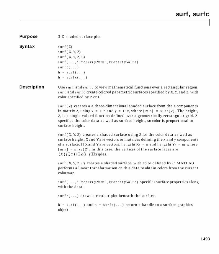
surf, surfc
1493
1surf, surfcPurpose 3-D shaded surface plot
Syntax surf(Z)surf(X,Y,Z)surf(X,Y,Z,C)surf(...,'PropertyName',PropertyValue)surfc(...)h = surf(...)h = surfc(...)
Description Use surf and surfc to view mathematical functions over a rectangular region.surf and surfc create colored parametric surfaces specified by X, Y, and Z, withcolor specified by Z or C.
surf(Z) creates a a three-dimensional shaded surface from the z componentsin matrix Z, using x = 1:n and y = 1:m, where [m,n] = size(Z). The height,Z, is a single-valued function defined over a geometrically rectangular grid. Zspecifies the color data as well as surface height, so color is proportional tosurface height.
surf(X,Y,Z) creates a shaded surface using Z for the color data as well assurface height. X and Y are vectors or matrices defining the x and y componentsof a surface. If X and Y are vectors, length(X) = n and length(Y) = m, where[m,n] = size(Z). In this case, the vertices of the surface faces are
triples.
surf(X,Y,Z,C) creates a shaded surface, with color defined by C. MATLABperforms a linear transformation on this data to obtain colors from the currentcolormap.
surf(...,'PropertyName',PropertyValue) specifies surface properties alongwith the data.
surfc(...) draws a contour plot beneath the surface.
h = surf(...) and h = surfc(...) return a handle to a surface graphicsobject.
X j( ) Y i( ) Z i j,( ), ,( )
surf, surfc
1494
Algorithm Abstractly, a parametric surface is parametrized by two independentvariables, i and j, which vary continuously over a rectangle; for example,1 ≤ i ≤ m and 1 ≤ j ≤ n. The three functions, x(i,j), y(i,j), and z(i,j),specify the surface. When i and j are integer values, they define a rectangulargrid with integer grid points. The functions x(i,j), y(i,j), and z(i,j)become three m-by-n matrices, X, Y and Z. surface color is a fourth function,c(i,j), denoted by matrix C.
Each point in the rectangular grid can be thought of as connected to its fournearest neighbors.
i–1,j |
i,j–1 – i,j – i,j+1 | i+1,j
This underlying rectangular grid induces four-sided patches on the surface. Toexpress this another way, [X(:) Y(:) Z(:)] returns a list of triples specifyingpoints in 3-space. Each interior point is connected to the four neighborsinherited from the matrix indexing. Points on the edge of the surface havethree neighbors; the four points at the corners of the grid have only twoneighbors. This defines a mesh of quadrilaterals or a quad-mesh.
Surface color can be specified in two different ways – at the vertices or at thecenters of each patch. In this general setting, the surface need not be asingle-valued function of x and y. Moreover, the four-sided surface patchesneed not be planar. For example, you can have surfaces defined in polar,cylindrical, and spherical coordinate systems.
The shading function sets the shading. If the shading is interp, C must be thesame size as X, Y, and Z; it specifies the colors at the vertices. The color withina surface patch is a bilinear function of the local coordinates. If the shading isfaceted (the default) or flat, C(i,j) specifies the constant color in the surfacepatch:
(i,j) – (i,j+1)| C(i,j) |
(i+1,j) – (i+1,j+1)
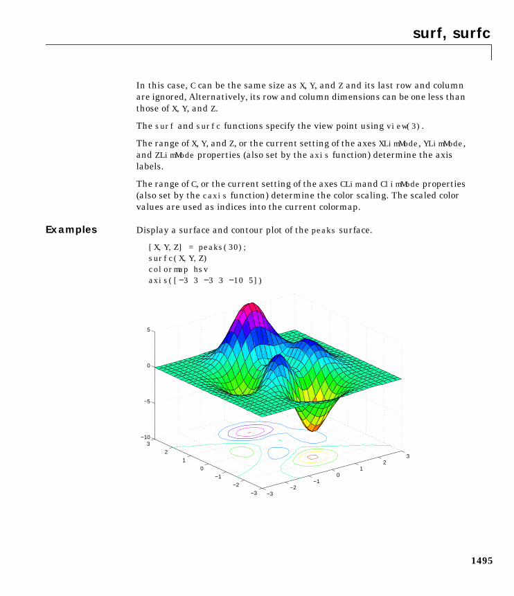
surf, surfc
1495
In this case, C can be the same size as X, Y, and Z and its last row and columnare ignored, Alternatively, its row and column dimensions can be one less thanthose of X, Y, and Z.
The surf and surfc functions specify the view point using view(3).
The range of X, Y, and Z, or the current setting of the axes XLimMode, YLimMode,and ZLimMode properties (also set by the axis function) determine the axislabels.
The range of C, or the current setting of the axes CLim and ClimMode properties(also set by the caxis function) determine the color scaling. The scaled colorvalues are used as indices into the current colormap.
Examples Display a surface and contour plot of the peaks surface.
[X,Y,Z] = peaks(30);surfc(X,Y,Z)colormap hsvaxis([−3 3 −3 3 −10 5])
−3−2
−10
12
3
−3
−2
−1
0
1
2
3−10
−5
0
5
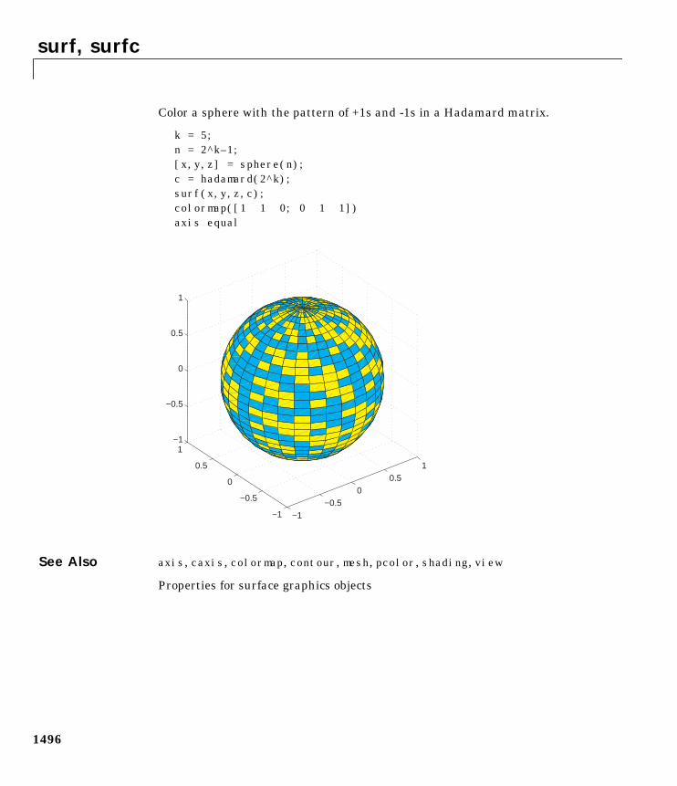
surf, surfc
1496
Color a sphere with the pattern of +1s and -1s in a Hadamard matrix.
k = 5;n = 2^k–1;[x,y,z] = sphere(n);c = hadamard(2^k);surf(x,y,z,c);colormap([1 1 0; 0 1 1])axis equal
See Also axis, caxis, colormap, contour, mesh, pcolor, shading, view
Properties for surface graphics objects
−1−0.5
00.5
1
−1
−0.5
0
0.5
1−1
−0.5
0
0.5
1
surf2patch
1497
1surf2patchPurpose Convert surface data to patch data
Syntax fvc = surf2patch(h)fvc = surf2patch(Z)fvc = surf2patch(Z,C)fvc = surf2patch(X,Y,Z)fvc = surf2patch(X,Y,Z,C)fvc = surf2patch(...,'triangles')[f,v,c] = surf2patch(...)
Description fvc = surf2patch(h) converts the geometry and color data from the surfaceobject identified by the handle h into patch format and returns the face, vertex,and color data in the struct fvc. You can pass this struct directly to the patchcommand.
fvc = surf2patch(Z) calculates the patch data from the surface’s ZDatamatrix Z.
fvc = surf2patch(Z,C) calculates the patch data from the surface’s ZData andCData matrices Z and C.
fvc = surf2patch(X,Y,Z) calculates the patch data from the surface’s XData,YData, and ZData matrices X, Y, and Z.
fvc = surf2patch(X,Y,Z,C) calculates the patch data from the surface’sXData, YData, ZData, and CData matrices X, Y, Z, and C.
fvc = surf2patch(...,'triangles') creates triangular faces instead of thequadrilaterals that compose surfaces.
[f,v,c] = surf2patch(...) returns the face, vertex, and color data in thethree arrays f, v, and c instead of a struct.
Examples The first example uses the sphere command to generate the XData, YData, andZData of a surface, which is then converted to a patch. Note that the ZData (z)is passed to surf2patch as both the third and fourth arguments – the thirdargument is the ZData and the fourth argument is taken as the CData. This isbecause the patch command does not automatically use the z-coordinate datafor the color data, as does the surface command.
surf2patch
1498
Also, because patch is a low-level command, you must set the view to 3-D andshading to faceted to produce the same results produced by the surfcommand.
[x y z] = sphere;patch(surf2patch(x,y,z,z));shading faceted; view(3)
In the second example surf2patch calculates face, vertex, and color data froma surface whose handle has been passed as an argument.
s = surf(peaks);pausepatch(surf2patch(s));delete(s)shading faceted; view(3)
See Also patch, reducepatch, shrinkfaces, surface, surf
surface
1499
1surfacePurpose Create surface object
Syntax surface(Z)surface(Z,C)surface(X,Y,Z)surface(X,Y,Z,C)surface(...'PropertyName',PropertyValue,...)h = surface(...)
Description surface is the low-level function for creating surface graphics objects. surfacesare plots of matrix data created using the row and column indices of eachelement as the x- and y-coordinates and the value of each element as thez-coordinate.
surface(Z) plots the surface specified by the matrix Z. Here, Z is asingle-valued function, defined over a geometrically rectangular grid.
surface(Z,C) plots the surface specified by Z and colors it according to thedata in C (see “Examples”).
surface(X,Y,Z) uses C = Z, so color is proportional to surface height above thex-y plane.
surface(X,Y,Z,C) plots the parametric surface specified by X, Y and Z, withcolor specified by C.
surface(x,y,Z), surface(x,y,Z,C) replaces the first two matrix argumentswith vectors and must have length(x) = n and length(y) = m where[m,n] = size(Z). In this case, the vertices of the surface facets are the triples(x(j),y(i),Z(i,j)). Note that x corresponds to the columns of Z and ycorresponds to the rows of Z. For a complete discussion of parametric surfaces,see the surf function.
surface(...'PropertyName',PropertyValue,...) follows the X, Y, Z, and Carguments with property name/property value pairs to specify additionalsurface properties. These properties are described in the “Surface Properties”section.
h = surface(...) returns a handle to the created surface object.
surface
1500
Remarks Unlike high-level area creation functions, such as surf or mesh, surface doesnot respect the settings of the figure and axes NextPlot properties. It simplyadds the surface object to the current axes.
If you do not specify separate color data (C), MATLAB uses the matrix (Z) todetermine the coloring of the surface. In this case, color is proportional tovalues of Z. You can specify a separate matrix to color the surfaceindependently of the data defining the area of the surface.
You can specify properties as property name/property value pairs, structurearrays, and cell arrays (see set and get for examples of how to specify thesedata types).
surface provides convenience forms that allow you to omit the property namefor the XData, YData, ZData, and CData properties. For example,
surface('XData',X,'YData',Y,'ZData',Z,'CData',C)
is equivalent to:
surface(X,Y,Z,C)
When you specify only a single matrix input argument,
surface(Z)
MATLAB assigns the data properties as if you specified,
surface('XData',[1:size(Z,2)],...'YData',[1:size(Z,1)],...'ZData',Z,...'CData',Z)
The axis, caxis, colormap, hold, shading, and view commands set graphicsproperties that affect surfaces. You can also set and query surface propertyvalues after creating them using the set and get commands.
Example This example creates a surface using the peaks M-file to generate the data, andcolors it using the clown image. The ZData is a 49-by-49 element matrix, while
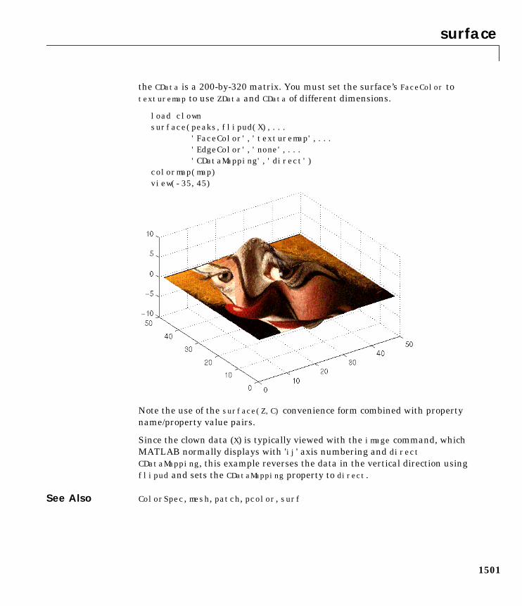
surface
1501
the CData is a 200-by-320 matrix. You must set the surface’s FaceColor totexturemap to use ZData and CData of different dimensions.
load clownsurface(peaks,flipud(X),...
'FaceColor','texturemap',...'EdgeColor','none',...'CDataMapping','direct')
colormap(map)view(-35,45)
Note the use of the surface(Z,C) convenience form combined with propertyname/property value pairs.
Since the clown data (X) is typically viewed with the image command, whichMATLAB normally displays with 'ij' axis numbering and directCDataMapping, this example reverses the data in the vertical direction usingflipud and sets the CDataMapping property to direct.
See Also ColorSpec, mesh, patch, pcolor, surf
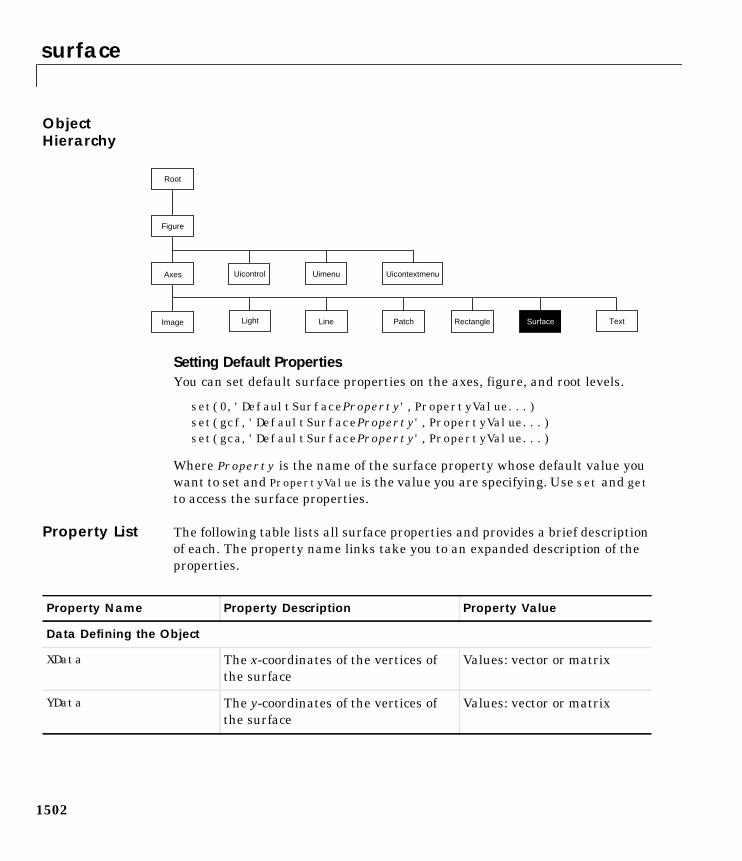
surface
1502
ObjectHierarchy
Setting Default PropertiesYou can set default surface properties on the axes, figure, and root levels.
set(0,'DefaultSurfaceProperty',PropertyValue...)set(gcf,'DefaultSurfaceProperty',PropertyValue...)set(gca,'DefaultSurfaceProperty',PropertyValue...)
Where Property is the name of the surface property whose default value youwant to set and PropertyValue is the value you are specifying. Use set and getto access the surface properties.
Property List The following table lists all surface properties and provides a brief descriptionof each. The property name links take you to an expanded description of theproperties.
Uimenu
Line
Axes Uicontrol
Image
Figure
Uicontextmenu
Light SurfacePatch Text
Root
Rectangle
Property Name Property Description Property Value
Data Defining the Object
XData The x-coordinates of the vertices ofthe surface
Values: vector or matrix
YData The y-coordinates of the vertices ofthe surface
Values: vector or matrix
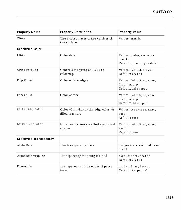
surface
1503
ZData The z-coordinates of the vertices ofthe surface
Values: matrix
Specifying Color
CData Color data Values: scalar, vector, ormatrixDefault: [] empty matrix
CDataMapping Controls mapping of CData tocolormap
Values: scaled, directDefault: scaled
EdgeColor Color of face edges Values: ColorSpec, none,flat, interpDefault: ColorSpec
FaceColor Color of face Values: ColorSpec, none,flat, interpDefault: ColorSpec
MarkerEdgeColor Color of marker or the edge color forfilled markers
Values: ColorSpec, none,autoDefault: auto
MarkerFaceColor Fill color for markers that are closedshapes
Values: ColorSpec, none,autoDefault: none
Specifying Transparency
AlphaData The transparency data m-by-n matrix of double oruint8
AlphaDataMapping Transparency mapping method none, direct, scaledDefault: scaled
EdgeAlpha Transparency of the edges of patchfaces
scalar, flat, interpDefault: 1 (opaque)
Property Name Property Description Property Value
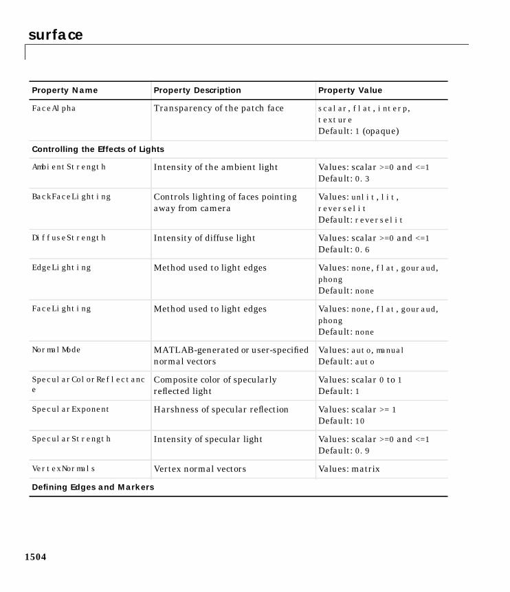
surface
1504
FaceAlpha Transparency of the patch face scalar, flat, interp,textureDefault: 1 (opaque)
Controlling the Effects of Lights
AmbientStrength Intensity of the ambient light Values: scalar >=0 and <=1Default: 0.3
BackFaceLighting Controls lighting of faces pointingaway from camera
Values: unlit, lit,reverselitDefault: reverselit
DiffuseStrength Intensity of diffuse light Values: scalar >=0 and <=1Default: 0.6
EdgeLighting Method used to light edges Values: none, flat, gouraud,phongDefault: none
FaceLighting Method used to light edges Values: none, flat, gouraud,phongDefault: none
NormalMode MATLAB-generated or user-specifiednormal vectors
Values: auto, manualDefault: auto
SpecularColorReflectance
Composite color of specularlyreflected light
Values: scalar 0 to 1Default: 1
SpecularExponent Harshness of specular reflection Values: scalar >= 1Default: 10
SpecularStrength Intensity of specular light Values: scalar >=0 and <=1Default: 0.9
VertexNormals Vertex normal vectors Values: matrix
Defining Edges and Markers
Property Name Property Description Property Value
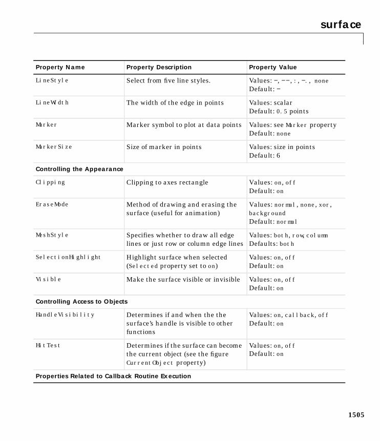
surface
1505
LineStyle Select from five line styles. Values: −, −− , :, −., noneDefault: −
LineWidth The width of the edge in points Values: scalarDefault: 0.5 points
Marker Marker symbol to plot at data points Values: see Marker propertyDefault: none
MarkerSize Size of marker in points Values: size in pointsDefault: 6
Controlling the Appearance
Clipping Clipping to axes rectangle Values: on, offDefault: on
EraseMode Method of drawing and erasing thesurface (useful for animation)
Values: normal, none, xor,backgroundDefault: normal
MeshStyle Specifies whether to draw all edgelines or just row or column edge lines
Values: both, row, columnDefaults: both
SelectionHighlight Highlight surface when selected(Selected property set to on)
Values: on, offDefault: on
Visible Make the surface visible or invisible Values: on, offDefault: on
Controlling Access to Objects
HandleVisibility Determines if and when the thesurface’s handle is visible to otherfunctions
Values: on, callback, offDefault: on
HitTest Determines if the surface can becomethe current object (see the figureCurrentObject property)
Values: on, offDefault: on
Properties Related to Callback Routine Execution
Property Name Property Description Property Value

surface
1506
BusyAction Specifies how to handle callbackroutine interruption
Values: cancel, queueDefault: queue
ButtonDownFcn Defines a callback routine thatexecutes when a mouse button ispressed on over the surface
Values: stringDefault: '' (empty string)
CreateFcn Defines a callback routine thatexecutes when an surface is created
Values: stringDefault: '' (empty string)
DeleteFcn Defines a callback routine thatexecutes when the surface is deleted(via close or delete)
Values: stringDefault: '' (empty string)
Interruptible Determines if callback routine can beinterrupted
Values: on, offDefault: on (can beinterrupted)
UIContextMenu Associates a context menu with thesurface
Values: handle of auicontextmenu
General Information About the Surface
Children Surface objects have no children Values: [] (empty matrix)
Parent The parent of a surface object isalways an axes object
Value: axes handle
Selected Indicates whether the surface is in a“selected” state.
Values: on, offDefault: on
Tag User-specified label Value: any stringDefault: '' (empty string)
Type The type of graphics object (readonly)
Value: the string 'surface'
UserData User-specified data Values: any matrixDefault: [] (empty matrix)
Property Name Property Description Property Value
Surface Properties
1507
1Surface PropertiesModifyingProperties
You can set and query graphics object properties in two ways:
• The Property Editor is an interactive tool that enables you to see and changeobject property values.
• The set and get commands enable you to set and query the values ofproperties
To change the default value of properties see Settingcreating_plots DefaultProperty Values.
SurfacePropertyDescriptions
This section lists property names along with the types of values each accepts.Curly braces enclose default values.
AlphaData m-by-n matrix of double or uint8
The transparency data. A matrix of non-NaN values specifying thetransparency of each face or vertex of the object. The AlphaData can be of classdouble or uint8.
MATLAB determines the transparency in one of three ways:
• Using the elements of AlphaData as transparency values (AlphaDataMappingset to none).
• Using the elements of AlphaData as indices into the current alphamap(AlphaDataMapping set to direct).
• Scaling the elements of AlphaData to range between the minimum andmaximum values of the axes ALim property (AlphaDataMapping set toscaled, the default).
AlphaDataMapping none | direct | scaled
Transparency mapping method. This property determines how MATLABinterprets indexed alpha data. This property can be any of the following:
• none - The transparency values of AlphaData are between 0 and 1 or areclamped to this range (the default).
• scaled - Transform the AlphaData to span the portion of the alphamapindicated by the axes ALim property, linearly mapping data values to alphavalues.
• direct - use the AlphaData as indices directly into the alphamap. When notscaled, the data are usually integer values ranging from 1 tolength(alphamap). MATLAB maps values less than 1 to the first alpha
Surface Properties
1508
value in the alphamap, and values greater than length(alphamap) to thelast alpha value in the alphamap. Values with a decimal portion are fixed tothe nearest, lower integer. If AlphaData is an array unit8 integers, then theindexing begins at 0 (i.e., MATLAB maps a value of 0 to the first alpha valuein the alphamap).
AmbientStrength scalar >= 0 and <= 1
Strength of ambient light. This property sets the strength of the ambient light,which is a nondirectional light source that illuminates the entire scene. Youmust have at least one visible light object in the axes for the ambient light tobe visible. The axes AmbientLightColor property sets the color of the ambientlight, which is therefore the same on all objects in the axes.
You can also set the strength of the diffuse and specular contribution of lightobjects. See the surface DiffuseStrength and SpecularStrength properties.
BackFaceLighting unlit | lit | reverselit
Face lighting control. This property determines how faces are lit when theirvertex normals point away from the camera.
• unlit – face is not lit
• lit – face lit in normal way
• reverselit – face is lit as if the vertex pointed towards the camera
This property is useful for discriminating between the internal and externalsurfaces of an object. See the Using MATLAB Graphics manual for an example.
BusyAction cancel | queue
Callback routine interruption. The BusyAction property enables you to controlhow MATLAB handles events that potentially interrupt executing callbackroutines. If there is a callback routine executing, subsequently invokedcallback routines always attempt to interrupt it. If the Interruptible propertyof the object whose callback is executing is set to on (the default), theninterruption occurs at the next point where the event queue is processed. If theInterruptible property is off, the BusyAction property (of the object owningthe executing callback) determines how MATLAB handles the event. Thechoices are:
Surface Properties
1509
• cancel – discard the event that attempted to execute a second callbackroutine.
• queue – queue the event that attempted to execute a second callback routineuntil the current callback finishes.
ButtonDownFcn string
Button press callback routine. A callback routine that executes whenever youpress a mouse button while the pointer is over the surface object. Define thisroutine as a string that is a valid MATLAB expression or the name of an M-file.The expression executes in the MATLAB workspace.
CData matrix
Vertex colors. A matrix containing values that specify the color at every pointin ZData. If you set the FaceColor property to texturemap, CData does not needto be the same size as ZData. In this case, MATLAB maps CData to conform tothe surface defined by ZData.
You can specify color as indexed values or true color. Indexed color dataspecifies a single value for each vertex. These values are either scaled to maplinearly into the current colormap (see caxis) or interpreted directly as indicesinto the colormap, depending on the setting of the CDataMapping property.
True color defines an RGB value for each vertex. If the coordinate data (XDatafor example) are contained in m-by-n matrices, then CDatamust be an m-by-n-3array. The first page contains the red components, the second the greencomponents, and the third the blue components of the colors.
On computer displays that cannot display true color (e.g., 8-bit displays),MATLAB uses dithering to approximate the RGB triples using the colors in thefigure’s Colormap and Dithermap. By default, Dithermap uses thecolorcube(64) colormap. You can also specify your own dithermap.
CDataMapping scaled | direct
Direct or scaled color mapping. This property determines how MATLABinterprets indexed color data used to color the surface. (If you use true colorspecification for CData, this property has no effect.)
Surface Properties
1510
• scaled – transform the color data to span the portion of the colormapindicated by the axes CLim property, linearly mapping data values to colors.See the caxis reference page for more information on this mapping.
• direct – use the color data as indices directly into the colormap. The colordata should then be integer values ranging from 1 to length(colormap).MATLAB maps values less than 1 to the first color in the colormap, andvalues greater than length(colormap) to the last color in the colormap.Values with a decimal portion are fixed to the nearest, lower integer.
Children matrix of handles
Always the empty matrix; surface objects have no children.
Clipping on | off
Clipping to axes rectangle. When Clipping is on, MATLAB does not display anyportion of the surface that is outside the axes rectangle.
CreateFcn string
Callback routine executed during object creation. This property defines acallback routine that executes when MATLAB creates a surface object. Youmust define this property as a default value for surfaces. For example, thestatement,
set(0,'DefaultSurfaceCreateFcn',...'set(gcf,''DitherMap'',my_dithermap)')
defines a default value on the root level that sets the figure DitherMap propertywhenever you create a surface object. MATLAB executes this routine aftersetting all surface properties. Setting this property on an existing surfaceobject has no effect.
The handle of the object whose CreateFcn is being executed is accessible onlythrough the root CallbackObject property, which you can query using gcbo.
DeleteFcn string
Delete surface callback routine. A callback routine that executes when youdelete the surface object (e.g., when you issue a delete command or clear theaxes or figure). MATLAB executes the routine before destroying the object’sproperties so these values are available to the callback routine.
The handle of the object whose DeleteFcn is being executed is accessible onlythrough the root CallbackObject property, which you can query using gcbo.
Surface Properties
1511
DiffuseStrength scalar >= 0 and <= 1
Intensity of diffuse light. This property sets the intensity of the diffusecomponent of the light falling on the surface. Diffuse light comes from lightobjects in the axes.
You can also set the intensity of the ambient and specular components of thelight on the surface object. See the AmbientStrength and SpecularStrengthproperties.
EdgeAlpha scalar = 1 | flat | interp
Transparency of the surface edges. This property can be any of the following:
• scalar - A single non-Nan scalar value between 0 and 1 that controls thetransparency of all the edges of the object. 1 (the default) is fully opaque and0 means completely transparent.
• flat - The alpha data (AlphaData) value for the first vertex of the facedetermines the transparency of the edges.
• interp - Linear interpolation of the alpha data (AlphaData) values at eachvertex determine the transparency of the edge.
Note that you must specify AlphaData as a matrix equal in size to ZData to useflat or interp EdgeAlpha.
EdgeColor ColorSpec | none | flat | interp
Color of the surface edge. This property determines how MATLAB colors theedges of the individual faces that make up the surface:
• ColorSpec — A three-element RGB vector or one of MATLAB’s predefinednames, specifying a single color for edges. The default EdgeColor is black.See ColorSpec for more information on specifying color.
• none — Edges are not drawn.
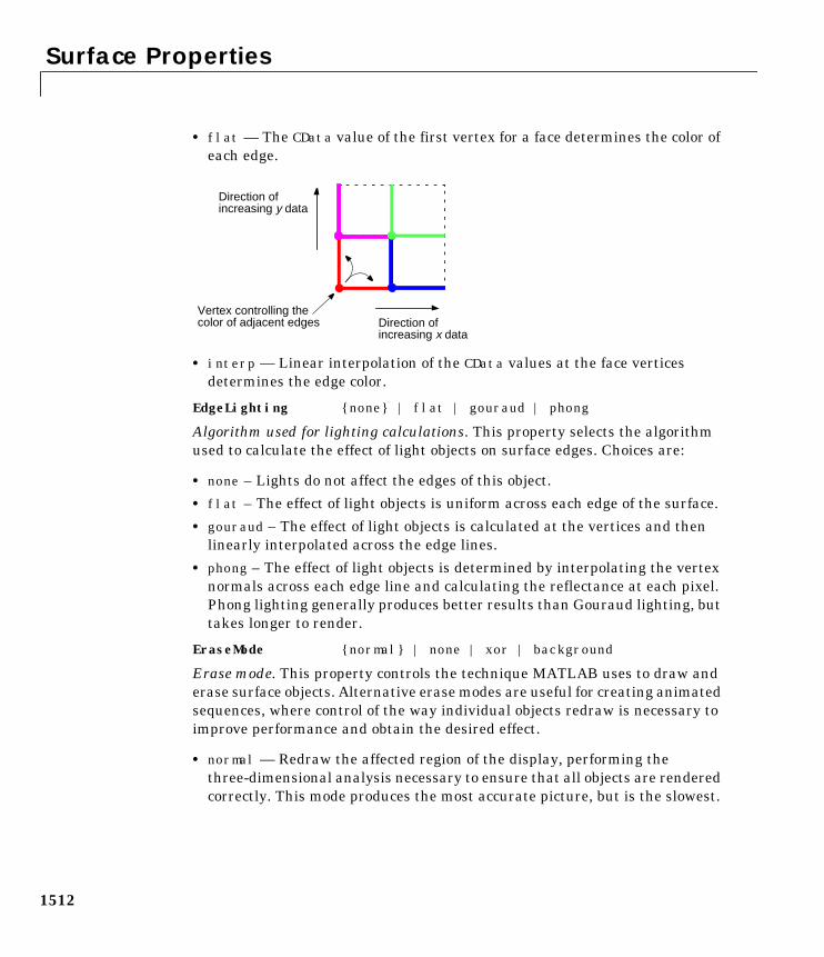
Surface Properties
1512
• flat — The CData value of the first vertex for a face determines the color ofeach edge.
• interp — Linear interpolation of the CData values at the face verticesdetermines the edge color.
EdgeLighting none | flat | gouraud | phong
Algorithm used for lighting calculations. This property selects the algorithmused to calculate the effect of light objects on surface edges. Choices are:
• none – Lights do not affect the edges of this object.
• flat – The effect of light objects is uniform across each edge of the surface.
• gouraud – The effect of light objects is calculated at the vertices and thenlinearly interpolated across the edge lines.
• phong – The effect of light objects is determined by interpolating the vertexnormals across each edge line and calculating the reflectance at each pixel.Phong lighting generally produces better results than Gouraud lighting, buttakes longer to render.
EraseMode normal | none | xor | background
Erase mode. This property controls the technique MATLAB uses to draw anderase surface objects. Alternative erase modes are useful for creating animatedsequences, where control of the way individual objects redraw is necessary toimprove performance and obtain the desired effect.
• normal — Redraw the affected region of the display, performing thethree-dimensional analysis necessary to ensure that all objects are renderedcorrectly. This mode produces the most accurate picture, but is the slowest.
Vertex controlling the
Direction of
Direction ofcolor of adjacent edges
increasing y data
increasing x data
Surface Properties
1513
The other modes are faster, but do not perform a complete redraw and aretherefore less accurate.
• none — Do not erase the surface when it is moved or destroyed. While theobject is still visible on the screen after erasing with EraseMode none, youcannot print it because MATLAB stores no information about its formerlocation.
• xor — Draw and erase the surface by performing an exclusive OR (XOR)with each pixel index of the screen behind it. Erasing the surface does notdamage the color of the objects behind it. However, surface color depends onthe color of the screen behind it and is correctly colored only when over theaxes background Color, or the figure background Color if the axes Color isset to none.
• background — Erase the surface by drawing it in the axes’ backgroundColor, or the figure background Color if the axes Color is set to none. Thisdamages objects that are behind the erased object, but surface objects arealways properly colored.
Printing with Non-normal Erase Modes. MATLAB always prints figures as if theEraseMode of all objects is normal. This means graphics objects created withEraseMode set to none, xor, or background can look different on screen than onpaper. On screen, MATLAB may mathematically combine layers of colors (e.g.,XORing a pixel color with that of the pixel behind it) and ignorethree-dimensional sorting to obtain greater rendering speed. However, thesetechniques are not applied to the printed output.
You can use the MATLAB getframe command or other screen captureapplication to create an image of a figure containing non-normal mode objects.
FaceAlpha scalar = 1 | flat | interp | texturemap
Transparency of the surface faces. This property can be any of the following:
• scalar - A single non-NaN scalar value between 0 and 1 that controls thetransparency of all the faces of the object. 1 (the default) is fully opaque and0 is completely transparent (invisible).
• flat - The values of the alpha data (AlphaData) determine the transparencyfor each face. The alpha data at the first vertex determines the transparencyof the entire face.
Surface Properties
1514
• interp - Bilinear interpolation of the alpha data (AlphaData) at each vertexdetermine the transparency of each face.
• texturemap – Use transparency for the texturemap.
Note that you must specify AlphaData as a matrix equal in size to ZData to useflat or interp FaceAlpha.
FaceColor ColorSpec | none | flat | interp
Color of the surface face. This property can be any of the following:
• ColorSpec — A three-element RGB vector or one of MATLAB’s predefinednames, specifying a single color for faces. See ColorSpec for moreinformation on specifying color.
• none — Do not draw faces. Note that edges are drawn independently of faces.
• flat — The values of CData determine the color for each face of the surface.The color data at the first vertex determines the color of the entire face.
• interp — Bilinear interpolation of the values at each vertex (the CData)determines the coloring of each face.
• texturemap — Texture map the CData to the surface. MATLAB transformsthe color data so that it conforms to the surface. (See the texture mappingexample.)
FaceLighting none | flat | gouraud | phong
Algorithm used for lighting calculations. This property selects the algorithmused to calculate the effect of light objects on the surface. Choices are:
• none – Lights do not affect the faces of this object.
• flat – The effect of light objects is uniform across the faces of the surface.Select this choice to view faceted objects.
• gouraud – The effect of light objects is calculated at the vertices and thenlinearly interpolated across the faces. Select this choice to view curvedsurfaces.
• phong – The effect of light objects is determined by interpolating the vertexnormals across each face and calculating the reflectance at each pixel. Selectthis choice to view curved surfaces. Phong lighting generally produces betterresults than Gouraud lighting, but takes longer to render.
Surface Properties
1515
HandleVisibility on | callback | off
Control access to object’s handle by command-line users and GUIs. Thisproperty determines when an object’s handle is visible in its parent’s list ofchildren. This property is useful for preventing command-line users fromaccidentally drawing into or deleting a figure that contains only user interfacedevices (such as a dialog box).
Handles are always visible when HandleVisibility is on.
Setting HandleVisibility to callback causes handles to be visible fromwithin callback routines or functions invoked by callback routines, but not fromwithin functions invoked from the command line. This provides a means toprotect GUIs from command-line users, while allowing callback routines tohave complete access to object handles.
Setting HandleVisibility to off makes handles invisible at all times. Thismay be necessary when a callback routine invokes a function that mightpotentially damage the GUI (such as evaluating a user-typed string), and sotemporarily hides its own handles during the execution of that function.
When a handle is not visible in its parent’s list of children, it cannot be returnedby functions that obtain handles by searching the object hierarchy or queryinghandle properties. This includes get, findobj, gca, gcf, gco, newplot, cla, clf,and close.
When a handle’s visibility is restricted using callback or off, the object’shandle does not appear in its parent’s Children property, figures do not appearin the root’s CurrentFigure property, objects do not appear in the root’sCallbackObject property or in the figure’s CurrentObject property, and axesdo not appear in their parent’s CurrentAxes property.
You can set the root ShowHiddenHandles property to on to make all handlesvisible, regardless of their HandleVisibility settings (this does not affect thevalues of the HandleVisibility properties).
Handles that are hidden are still valid. If you know an object’s handle, you canset and get its properties, and pass it to any function that operates on handles.
HitTest on | off
Selectable by mouse click. HitTest determines if the surface can become thecurrent object (as returned by the gco command and the figure CurrentObject
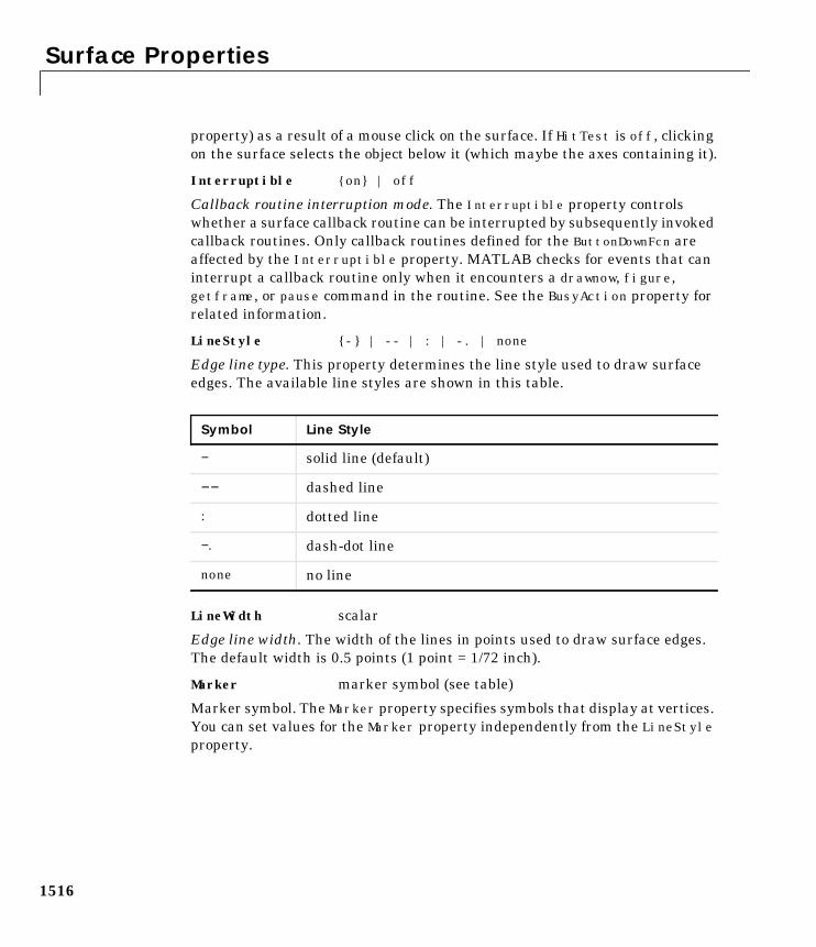
Surface Properties
1516
property) as a result of a mouse click on the surface. If HitTest is off, clickingon the surface selects the object below it (which maybe the axes containing it).
Interruptible on | off
Callback routine interruption mode. The Interruptible property controlswhether a surface callback routine can be interrupted by subsequently invokedcallback routines. Only callback routines defined for the ButtonDownFcn areaffected by the Interruptible property. MATLAB checks for events that caninterrupt a callback routine only when it encounters a drawnow, figure,getframe, or pause command in the routine. See the BusyAction property forrelated information.
LineStyle - | -- | : | -. | none
Edge line type. This property determines the line style used to draw surfaceedges. The available line styles are shown in this table.
LineWidth scalar
Edge line width. The width of the lines in points used to draw surface edges.The default width is 0.5 points (1 point = 1/72 inch).
Marker marker symbol (see table)
Marker symbol. The Marker property specifies symbols that display at vertices.You can set values for the Marker property independently from the LineStyleproperty.
Symbol Line Style
− solid line (default)
−− dashed line
: dotted line
−. dash-dot line
none no line
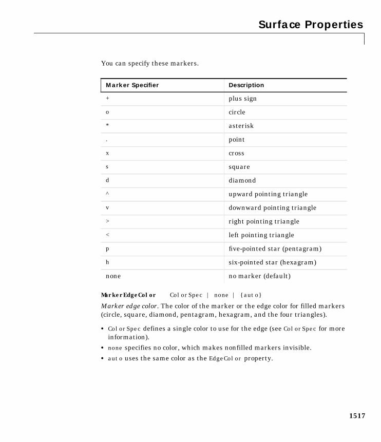
Surface Properties
1517
You can specify these markers.
MarkerEdgeColor ColorSpec | none | auto
Marker edge color. The color of the marker or the edge color for filled markers(circle, square, diamond, pentagram, hexagram, and the four triangles).
• ColorSpec defines a single color to use for the edge (see ColorSpec for moreinformation).
• none specifies no color, which makes nonfilled markers invisible.
• auto uses the same color as the EdgeColor property.
Marker Specifier Description
+ plus sign
o circle
* asterisk
. point
x cross
s square
d diamond
^ upward pointing triangle
v downward pointing triangle
> right pointing triangle
< left pointing triangle
p five-pointed star (pentagram)
h six-pointed star (hexagram)
none no marker (default)
Surface Properties
1518
MarkerFaceColor ColorSpec | none | auto
Marker face color. The fill color for markers that are closed shapes (circle,square, diamond, pentagram, hexagram, and the four triangles).
• ColorSpec defines a single color to use for all marker on the surface (seeColorSpec for more information).
• none makes the interior of the marker transparent, allowing the backgroundto show through.
• auto uses the CData for the vertex located by the marker to determine thecolor.
MarkerSize size in points
Marker size. A scalar specifying the marker size, in points. The default valuefor MarkerSize is six points (1 point = 1/72 inch). Note that MATLAB draws thepoint marker at 1/3 the specified marker size.
MeshStyle both | row | column
Row and column lines. This property specifies whether to draw all edge linesor just row or column edge lines.
• both draws edges for both rows and columns.
• row draws row edges only.
• column draws column edges only.
NormalMode auto | manual
MATLAB -generated or user-specified normal vectors. When this property isauto, MATLAB calculates vertex normals based on the coordinate data. If youspecify your own vertex normals, MATLAB sets this property to manual anddoes not generate its own data. See also the VertexNormals property.
Parent handle
Surface’s parent object. The parent of a surface object is the axes in which it isdisplayed. You can move a surface object to another axes by setting thisproperty to the handle of the new parent.
Selected on | off
Is object selected? When this property is on, MATLAB displays a dashedbounding box around the surface if the SelectionHighlight property is also
Surface Properties
1519
on. You can, for example, define the ButtonDownFcn to set this property,allowing users to select the object with the mouse.
SelectionHighlight on | off
Objects highlight when selected. When the Selected property is on, MATLABindicates the selected state by drawing a dashed bounding box around thesurface. When SelectionHighlight is off, MATLAB does not draw thehandles.
SpecularColorReflectancescalar in the range 0 to 1
Color of specularly reflected light. When this property is 0, the color of thespecularly reflected light depends on both the color of the object from which itreflects and the color of the light source. When set to 1, the color of thespecularly reflected light depends only on the color or the light source (i.e., thelight object Color property). The proportions vary linearly for values inbetween.
SpecularExponent scalar >= 1
Harshness of specular reflection. This property controls the size of the specularspot. Most materials have exponents in the range of 5 to 20.
SpecularStrength scalar >= 0 and <= 1
Intensity of specular light. This property sets the intensity of the specularcomponent of the light falling on the surface. Specular light comes from lightobjects in the axes.
You can also set the intensity of the ambient and diffuse components of thelight on the surface object. See the AmbientStrength and DiffuseStrengthproperties. Also see the material function.
Tag string
User-specified object label. The Tag property provides a means to identifygraphics objects with a user-specified label. This is particularly useful whenconstructing interactive graphics programs that would otherwise need todefine object handles as global variables or pass them as arguments betweencallback routines. You can define Tag as any string.
Type string (read only)
Class of the graphics object. The class of the graphics object. For surface objects,Type is always the string 'surface'.
Surface Properties
1520
UIContextMenu handle of a uicontextmenu object
Associate a context menu with the surface. Assign this property the handle of auicontextmenu object created in the same figure as the surface. Use theuicontextmenu function to create the context menu. MATLAB displays thecontext menu whenever you right-click over the surface.
UserData matrix
User-specified data. Any matrix you want to associate with the surface object.MATLAB does not use this data, but you can access it using the set and getcommands.
VertexNormals vector or matrix
Surface normal vectors. This property contains the vertex normals for thesurface. MATLAB generates this data to perform lighting calculations. You cansupply your own vertex normal data, even if it does not match the coordinatedata. This can be useful to produce interesting lighting effects.
Visible on | off
Surface object visibility. By default, all surfaces are visible. When set to off,the surface is not visible, but still exists and you can query and set itsproperties.
XData vector or matrix
X-coordinates. The x-position of the surface points. If you specify a row vector,surface replicates the row internally until it has the same number of columnsas ZData.
YData vector or matrix
Y-coordinates. The y-position of the surface points. If you specify a row vector,surface replicates the row internally until it has the same number of rows asZData.
ZData matrix
Z-coordinates. Z-position of the surface points. See the Description section formore information.
surfl
1521
1surflPurpose Surface plot with colormap-based lighting
Syntax surfl(Z)surfl(X,Y,Z)surfl(...,'light')surfl(...,s)surfl(X,Y,Z,s,k)h = surfl(...)
Description The surfl function displays a shaded surface based on a combination ofambient, diffuse, and specular lighting models.
surfl(Z) and surfl(X,Y,Z) create three-dimensional shaded surfaces usingthe default direction for the light source and the default lighting coefficients forthe shading model. X, Y, and Z are vectors or matrices that define the x, y, andz components of a surface.
surfl(...,'light') produces a colored, lighted surface using a MATLABlight object. This produces results different from the default lighting method,surfl(...,'cdata'), which changes the color data for the surface to be thereflectance of the surface.
surfl(...,s) specifies the direction of the light source. s is a two- orthree-element vector that specifies the direction from a surface to a lightsource. s = [sx sy sz] or s = [azimuth elevation]. The default s is 45˚counterclockwise from the current view direction.
surfl(X,Y,Z,s,k) specifies the reflectance constant. k is a four-element vectordefining the relative contributions of ambient light, diffuse reflection, specularreflection, and the specular shine coefficient. k = [ka kd ks shine] anddefaults to [.55,.6,.4,10].
h = surfl(...) returns a handle to a surface graphics object.
Remarks For smoother color transitions, use colormaps that have linear intensityvariations (e.g., gray, copper, bone, pink).
The ordering of points in the X, Y, and Z matrices define the inside and outsideof parametric surfaces. If you want the opposite side of the surface to reflect the
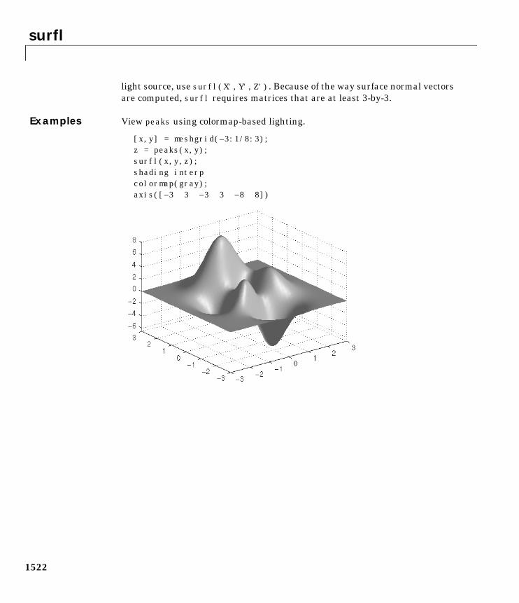
surfl
1522
light source, use surfl(X',Y',Z'). Because of the way surface normal vectorsare computed, surfl requires matrices that are at least 3-by-3.
Examples View peaks using colormap-based lighting.
[x,y] = meshgrid(–3:1/8:3);z = peaks(x,y);surfl(x,y,z);shading interpcolormap(gray);axis([–3 3 –3 3 –8 8])
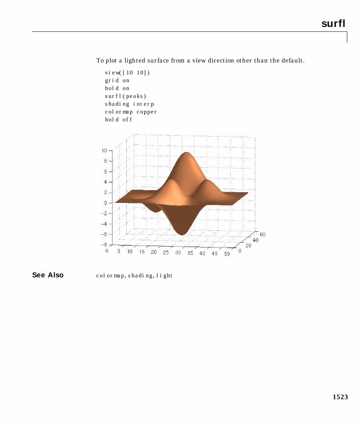
surfl
1523
To plot a lighted surface from a view direction other than the default.
view([10 10])grid onhold onsurfl(peaks)shading interpcolormap copperhold off
See Also colormap, shading, light
surfnorm
1524
1surfnormPurpose Compute and display 3-D surface normals
Syntax surfnorm(Z)surfnorm(X,Y,Z)[Nx,Ny,Nz] = surfnorm(...)
Description The surfnorm function computes surface normals for the surface defined by X,Y, and Z. The surface normals are unnormalized and valid at each vertex.Normals are not shown for surface elements that face away from the viewer.
surfnorm(Z) and surfnorm(X,Y,Z) plot a surface and its surface normals. Z isa matrix that defines the z component of the surface. X and Y are vectors ormatrices that define the x and y components of the surface.
[Nx,Ny,Nz] = surfnorm(...) returns the components of thethree-dimensional surface normals for the surface.
Remarks The direction of the normals is reversed by calling surfnorm with transposedarguments:
surfnorm(X',Y',Z')
surfl uses surfnorm to compute surface normals when calculating thereflectance of a surface.
Algorithm The surface normals are based on a bicubic fit of the data in X, Y, and Z. Foreach vertex, diagonal vectors are computed and crossed to form the normal.
Examples Plot the normal vectors for a truncated cone.
[x,y,z] = cylinder(1:10);surfnorm(x,y,z)axis([−12 12 −12 12 −0.1 1])
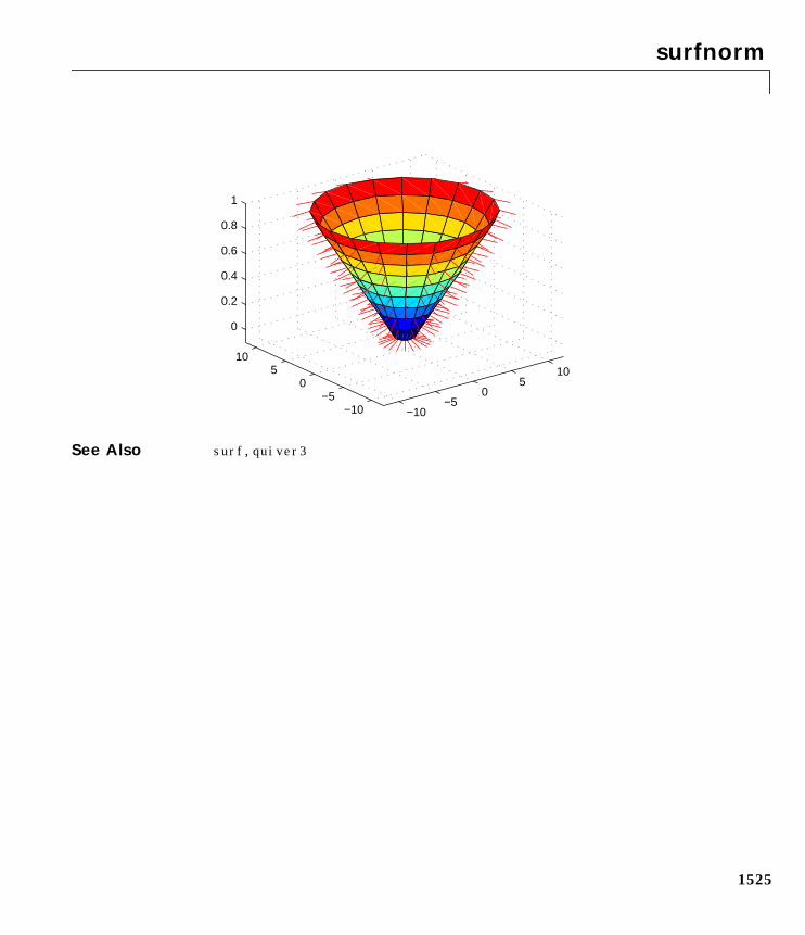
surfnorm
1525
See Also surf, quiver3
−10−5
05
10
−10−5
05
10
0
0.2
0.4
0.6
0.8
1
svd
1526
1svdPurpose Singular value decomposition
Syntax s = svd(X)[U,S,V] = svd(X)[U,S,V] = svd(X,0)
Description The svd command computes the matrix singular value decomposition.
s = svd(X) returns a vector of singular values.
[U,S,V] = svd(X) produces a diagonal matrix S of the same dimension as X,with nonnegative diagonal elements in decreasing order, and unitary matricesU and V so that X = U*S*V'.
[U,S,V] = svd(X,0) produces the “economy size” decomposition. If X is m-by-nwith m > n, then svd computes only the first n columns of U and S is n-by-n.
Examples For the matrix
X =1 23 45 67 8
the statement
[U,S,V] = svd(X)
produces
U =-0.1525 -0.8226 -0.3945 -0.3800-0.3499 -0.4214 0.2428 0.8007-0.5474 -0.0201 0.6979 -0.4614-0.7448 0.3812 -0.5462 0.0407
S =14.2691 0
0 0.6268
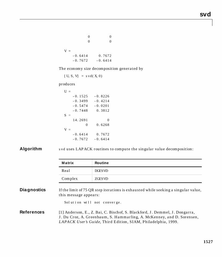
svd
1527
0 00 0
V =-0.6414 0.7672-0.7672 -0.6414
The economy size decomposition generated by
[U,S,V] = svd(X,0)
produces
U =-0.1525 -0.8226-0.3499 -0.4214-0.5474 -0.0201-0.7448 0.3812
S =14.2691 0
0 0.6268V =
-0.6414 0.7672-0.7672 -0.6414
Algorithm svd uses LAPACK routines to compute the singular value decomposition:
Diagnostics If the limit of 75 QR step iterations is exhausted while seeking a singular value,this message appears:
Solution will not converge.
References [1] Anderson, E., Z. Bai, C. Bischof, S. Blackford, J. Demmel, J. Dongarra,J. Du Croz, A. Greenbaum, S. Hammarling, A. McKenney, and D. Sorensen,LAPACK User’s Guide, Third Edition, SIAM, Philadelphia, 1999.
Matrix Routine
Real DGESVD
Complex ZGESVD
svds
1528
1svdsPurpose A few singular values
Syntax s = svds(A)s = svds(A,k)s = svds(A,k,0)[U,S,V] = svds(A,...)
Description svds(A) computes the five largest singular values and associated singularvectors of the matrix A.
svds(A,k) computes the k largest singular values and associated singularvectors of the matrix A.
svds(A,k,0) computes the k smallest singular values and associated singularvectors.
With one output argument, s is a vector of singular values. With three outputarguments and if A is m-by-n:
• U is m-by-k with orthonormal columns
• S is k-by-k diagonal
• V is n-by-k with orthonormal columns
• U*S*V' is the closest rank k approximation to A
Algorithm svds(A,k) uses eigs to find the k largest magnitude eigenvalues andcorresponding eigenvectors of B = [0 A; A' 0].
svds(A,k,0) uses eigs to find the 2k smallest magnitude eigenvalues andcorresponding eigenvectors of B = [0 A; A' 0], and then selects the k positiveeigenvalues and their eigenvectors.
Example west0479 is a real 479-by-479 sparse matrix. svd calculates all 479 singularvalues. svds picks out the largest and smallest singular values.
load west0479s = svd(full(west0479))sl = svds(west0479,4)ss = svds(west0479,6,0)
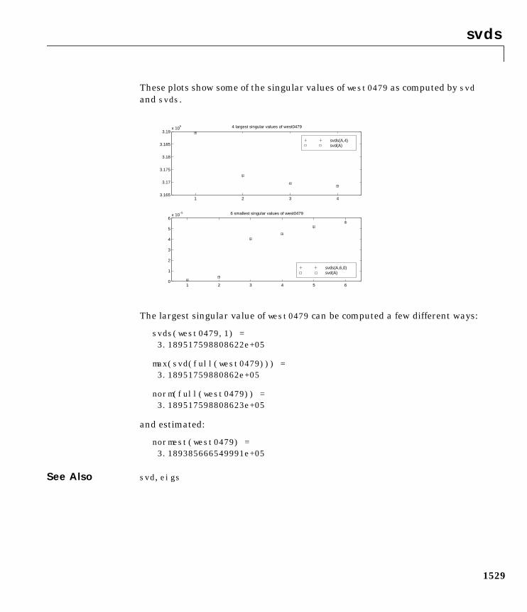
svds
1529
These plots show some of the singular values of west0479 as computed by svdand svds.
The largest singular value of west0479 can be computed a few different ways:
svds(west0479,1) = 3.189517598808622e+05
max(svd(full(west0479))) = 3.18951759880862e+05
norm(full(west0479)) = 3.189517598808623e+05
and estimated:
normest(west0479) = 3.189385666549991e+05
See Also svd, eigs
1 2 3 43.165
3.17
3.175
3.18
3.185
3.19x 10
5 4 largest singular values of west0479
svds(A,4)svd(A)
1 2 3 4 5 60
1
2
3
4
5
6x 10
−5 6 smallest singular values of west0479
svds(A,6,0)svd(A)
switch
1530
1switchPurpose Switch among several cases based on expression
Syntax switch switch_exprcase case_expr
statement,...,statementcase case_expr1,case_expr2,case_expr3,...
statement,...,statement...otherwise
statement,...,statementend
Discussion The switch statement syntax is a means of conditionally executing code. Inparticular, switch executes one set of statements selected from an arbitrarynumber of alternatives. Each alternative is called a case, and consists of:
• The case statement
• One or more case expressions
• One or more statements
In its basic syntax, switch executes the statements associated with the firstcase where switch_expr == case_expr. When the case expression is a cellarray (as in the second case above), the case_expr matches if any of theelements of the cell array match the switch expression. If no case expressionmatches the switch expression, then control passes to the otherwise case (if itexists). After the case is executed, program execution resumes with thestatement after the end.
The switch_expr can be a scalar or a string. A scalar switch_expr matches acase_expr if switch_expr==case_expr. A string switch_expr matches acase_expr if strcmp(switch_expr,case_expr) returns 1 (true).
Note for C Programmers Unlike the C language switch construct,MATLAB’s switch does not “fall through.” That is, switch executes only thefirst matching case, subsequent matching cases do not execute. Therefore,break statements are not used.
switch
1531
Examples Assume method exists as a string variable:
switch lower(method)case 'linear','bilinear', disp('Method is linear')case 'cubic', disp('Method is cubic')case 'nearest', disp('Method is nearest')otherwise, disp('Unknown method.')
end
See Also case, end, if, otherwise, while
symamd
1532
1symamdPurpose Symmetric approximate minimum degree permutation
Syntax p = symamd(S)p = symamd(S,knobs)[p,stats] = symamd(S)[p,stats] = symamd(S,knobs)
Description p = symamd(S) for a symmetric positive definite matrix S, returns thepermutation vector p such that S(p,p) tends to have a sparser Cholesky factorthan S. To find the ordering for S, symamd constructs a matrix M such thatspones(M'*M) = spones (S), and then computes p = colamd(M). The symamdfunction may also work well for symmetric indefinite matrices.
S must be square; only the strictly lower triangular part is referenced.
knobs is a scalar. If S is n-by-n, rows and columns with more than knobs*nentries are removed prior to ordering, and ordered last in the outputpermutation p. If the knobs parameter is not present, thenknobs = spparms('wh_frac').
stats is an optional vector that provides data about the ordering and thevalidity of the matrix S.
stats(1) Number of dense or empty rows ignored by symamd
stats(2) Number of dense or empty columns ignored by symamd
stats(3) Number of garbage collections performed on the internal datastructure used by symamd (roughly of size8.4*nnz(tril(S,-1)) + 9n integers)
stats(4) 0 if the matrix is valid, or 1 if invalid
stats(5) Rightmost column index that is unsorted or contains duplicateentries, or 0 if no such column exists
stats(6) Last seen duplicate or out-of-order row index in the columnindex given by stats(5), or 0 if no such row index exists
stats(7) Number of duplicate and out-of-order row indices
symamd
1533
Although, MATLAB built-in functions generate valid sparse matrices, a usermay construct an invalid sparse matrix using the MATLAB C or Fortran APIsand pass it to symamd. For this reason, symamd verifies that S is valid:
• If a row index appears two or more times in the same column, symamd ignoresthe duplicate entries, continues processing, and provides information aboutthe duplicate entries in stats(4:7).
• If row indices in a column are out of order, symamd sorts each column of itsinternal copy of the matrix S (but does not repair the input matrix S),continues processing, and provides information about the out-of-orderentries in stats(4:7).
• If S is invalid in any other way, symamd cannot continue. It prints an errormessage, and returns no output arguments (p or stats) .
The ordering is followed by a symmetric elimination tree post-ordering.
Note symamd tends to be faster than symmmd and tends to return a betterordering.
See Also colamd, colmmd, colperm, spparms, symmmd, symrcm
References The authors of the code for symamd are Stefan I. Larimore and Timothy A. Davis([email protected]), University of Florida. The algorithm was developed incollaboration with John Gilbert, Xerox PARC, and Esmond Ng, Oak RidgeNational Laboratory. Sparse Matrix Algorithms Research at the University ofFlorida: http://www.cise.ufl.edu/research/sparse/
symbfact
1534
1symbfactPurpose Symbolic factorization analysis
Syntax count = symbfact(A)count = symbfact(A,'col')count = symbfact(A,'sym')[count,h,parent,post,R] = symbfact(...)
Description count = symbfact(A) returns the vector of row counts for the uppertriangular Cholesky factor of a symmetric matrix whose upper triangle is thatof A, assuming no cancellation during the factorization. symbfact should bemuch faster than chol(A).
count = symbfact(A,'col') analyzes A' ∗ A (without forming it explicitly).
count = symbfact(A,'sym') is the same as count = symbfact(A).
[count,h,parent,post,R] = symbfact(...) has several optional returnvalues.
See Also chol, etree, treelayout
h Height of the elimination tree
parent The elimination tree itself
post Postordering permutation of the elimination tree
R 0-1 matrix whose structure is that of chol(A)
symmlq
1535
1symmlqPurpose Symmetric LQ method
Syntax x = symmlq(A,b)symmlq(A,b,tol)symmlq(A,b,tol,maxit)symmlq(A,b,tol,maxit,M)symmlq(A,b,tol,maxit,M1,M2)symmlq(A,b,tol,maxit,M1,M2,x0)symmlq(afun,b,tol,maxit,m1fun,m2fun,x0,p1,p2,...)[x,flag] = symmlq(A,b,...)[x,flag,relres] = symmlq(A,b,...)[x,flag,relres,iter] = symmlq(A,b,...)[x,flag,relres,iter,resvec] = symmlq(A,b,...)[x,flag,relres,iter,resvec,resveccg] = symmlq(A,b,...)
Description x = symmlq(A,b) attempts to solve the system of linear equations A*x=b for x.The n-by-n coefficient matrix A must be symmetric but need not be positivedefinite. The column vector b must have length n. A can be a function afunsuch that afun(x) returns A*x.
If symmlq converges, a message to that effect is displayed. If symmlq fails toconverge after the maximum number of iterations or halts for any reason, awarning message is printed displaying the relative residual norm(b-A*x)/norm(b) and the iteration number at which the method stopped or failed.
symmlq(A,b,tol) specifies the tolerance of the method. If tol is [], thensymmlq uses the default, 1e-6.
symmlq(A,b,tol,maxit) specifies the maximum number of iterations. Ifmaxit is [], then symmlq uses the default, min(n,20).
symmlq(A,b,tol,maxit,M) and symmlq(A,b,tol,maxit,M1,M2) use thesymmetric positive definite preconditioner M or M = M1*M2 and effectively solvethe system inv(sqrt(M))*A*inv(sqrt(M))*y = inv(sqrt(M))*b for y andthen return x = inv(sqrt(M))*y. If M is [] then symmlq applies nopreconditioner. M can be a function that returns M\x.
symmlq(A,b,tol,maxit,M1,M2,x0) specifies the initial guess. If x0 is [], thensymmlq uses the default, an all-zero vector.
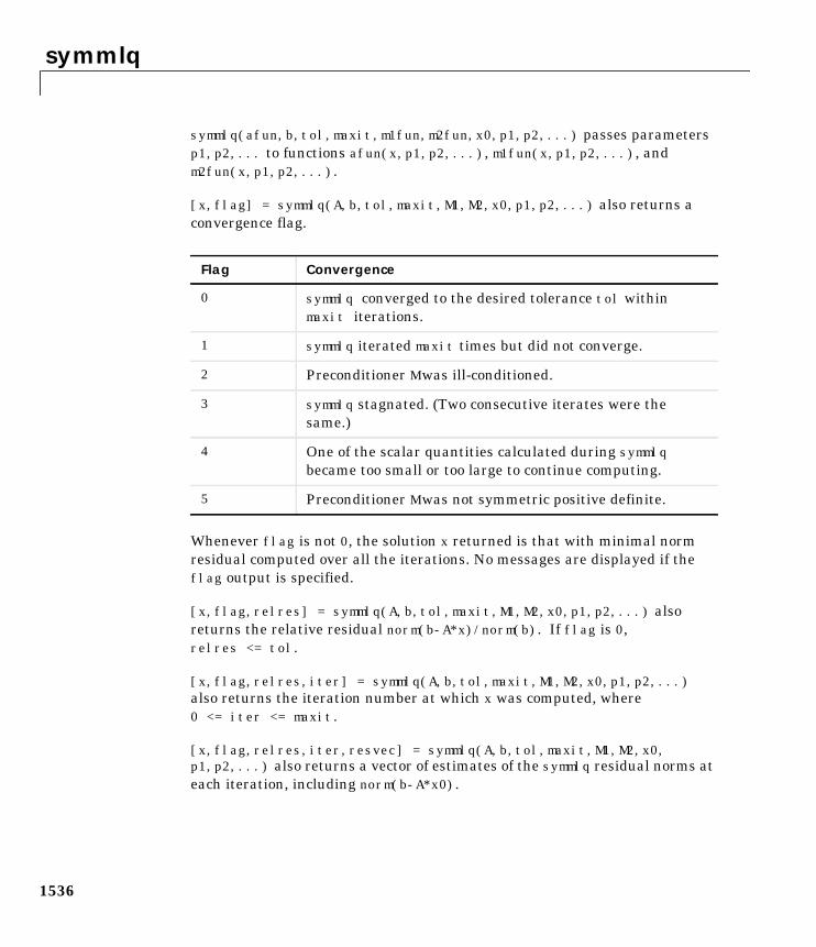
symmlq
1536
symmlq(afun,b,tol,maxit,m1fun,m2fun,x0,p1,p2,...) passes parametersp1,p2,... to functions afun(x,p1,p2,...), m1fun(x,p1,p2,...), andm2fun(x,p1,p2,...).
[x,flag] = symmlq(A,b,tol,maxit,M1,M2,x0,p1,p2,...) also returns aconvergence flag.
Whenever flag is not 0, the solution x returned is that with minimal normresidual computed over all the iterations. No messages are displayed if theflag output is specified.
[x,flag,relres] = symmlq(A,b,tol,maxit,M1,M2,x0,p1,p2,...) alsoreturns the relative residual norm(b-A*x)/norm(b). If flag is 0,relres <= tol.
[x,flag,relres,iter] = symmlq(A,b,tol,maxit,M1,M2,x0,p1,p2,...)also returns the iteration number at which x was computed, where0 <= iter <= maxit.
[x,flag,relres,iter,resvec] = symmlq(A,b,tol,maxit,M1,M2,x0,p1,p2,...) also returns a vector of estimates of the symmlq residual norms ateach iteration, including norm(b-A*x0).
Flag Convergence
0 symmlq converged to the desired tolerance tol withinmaxit iterations.
1 symmlq iterated maxit times but did not converge.
2 Preconditioner M was ill-conditioned.
3 symmlq stagnated. (Two consecutive iterates were thesame.)
4 One of the scalar quantities calculated during symmlqbecame too small or too large to continue computing.
5 Preconditioner M was not symmetric positive definite.
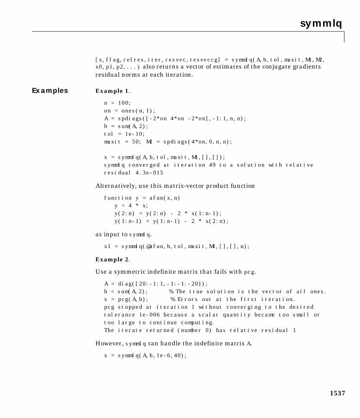
symmlq
1537
[x,flag,relres,iter,resvec,resveccg] = symmlq(A,b,tol,maxit,M1,M2,x0,p1,p2,...) also returns a vector of estimates of the conjugate gradientsresidual norms at each iteration.
Examples Example 1.
n = 100;on = ones(n,1);A = spdiags([-2*on 4*on -2*on],-1:1,n,n);b = sum(A,2);tol = 1e-10;maxit = 50; M1 = spdiags(4*on,0,n,n);
x = symmlq(A,b,tol,maxit,M1,[],[]);symmlq converged at iteration 49 to a solution with relativeresidual 4.3e-015
Alternatively, use this matrix-vector product function
function y = afun(x,n) y = 4 * x; y(2:n) = y(2:n) - 2 * x(1:n-1); y(1:n-1) = y(1:n-1) - 2 * x(2:n);
as input to symmlq.
x1 = symmlq(@afun,b,tol,maxit,M1,[],[],n);
Example 2.
Use a symmetric indefinite matrix that fails with pcg.
A = diag([20:-1:1,-1:-1:-20]);b = sum(A,2); % The true solution is the vector of all ones.x = pcg(A,b); % Errors out at the first iteration.pcg stopped at iteration 1 without converging to the desiredtolerance 1e-006 because a scalar quantity became too small ortoo large to continue computing.The iterate returned (number 0) has relative residual 1
However, symmlq can handle the indefinite matrix A.
x = symmlq(A,b,1e-6,40);
symmlq
1538
symmlq converged at iteration 39 to a solution with relativeresidual 1.3e-007
See Also bicg, bicgstab, cgs, lsqr, gmres, minres, pcg, qmr
@ (function handle), / (slash)
References [1] Barrett, R., M. Berry, T. F. Chan, et al., Templates for the Solution of LinearSystems: Building Blocks for Iterative Methods, SIAM, Philadelphia, 1994.
[2] Paige, C. C. and M. A., “Solution of Sparse Indefinite Systems of LinearEquations.” SIAM J. Numer. Anal., Vol.12, 1975, pp. 617-629.
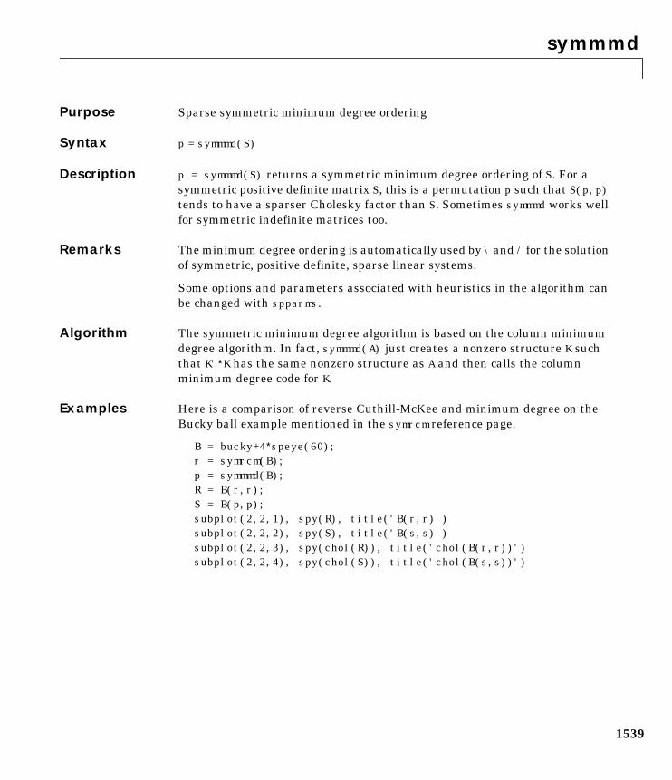
symmmd
1539
1symmmdPurpose Sparse symmetric minimum degree ordering
Syntax p = symmmd(S)
Description p = symmmd(S) returns a symmetric minimum degree ordering of S. For asymmetric positive definite matrix S, this is a permutation p such that S(p,p)tends to have a sparser Cholesky factor than S. Sometimes symmmd works wellfor symmetric indefinite matrices too.
Remarks The minimum degree ordering is automatically used by \ and / for the solutionof symmetric, positive definite, sparse linear systems.
Some options and parameters associated with heuristics in the algorithm canbe changed with spparms.
Algorithm The symmetric minimum degree algorithm is based on the column minimumdegree algorithm. In fact, symmmd(A) just creates a nonzero structure K suchthat K'∗K has the same nonzero structure as A and then calls the columnminimum degree code for K.
Examples Here is a comparison of reverse Cuthill-McKee and minimum degree on theBucky ball example mentioned in the symrcm reference page.
B = bucky+4∗speye(60);r = symrcm(B);p = symmmd(B);R = B(r,r);S = B(p,p);subplot(2,2,1), spy(R), title('B(r,r)')subplot(2,2,2), spy(S), title('B(s,s)')subplot(2,2,3), spy(chol(R)), title('chol(B(r,r))')subplot(2,2,4), spy(chol(S)), title('chol(B(s,s))')
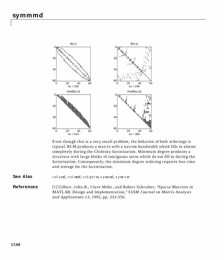
symmmd
1540
Even though this is a very small problem, the behavior of both orderings istypical. RCM produces a matrix with a narrow bandwidth which fills in almostcompletely during the Cholesky factorization. Minimum degree produces astructure with large blocks of contiguous zeros which do not fill in during thefactorization. Consequently, the minimum degree ordering requires less timeand storage for the factorization.
See Also colamd, colmmd, colperm, symamd, symrcm
References [1] Gilbert, John R., Cleve Moler, and Robert Schreiber, “Sparse Matrices inMATLAB: Design and Implementation,” SIAM Journal on Matrix Analysisand Applications 13, 1992, pp. 333-356.
0 20 40 60
0
20
40
60
nz = 240
B(r,r)
0 20 40 60
0
20
40
60
nz = 240
B(s,s)
0 20 40 60
0
20
40
60
nz = 514
chol(B(r,r))
0 20 40 60
0
20
40
60
nz = 360
chol(B(s,s))
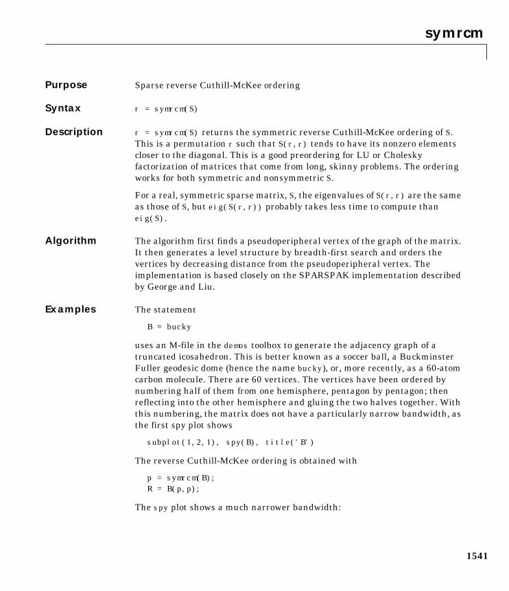
symrcm
1541
1symrcmPurpose Sparse reverse Cuthill-McKee ordering
Syntax r = symrcm(S)
Description r = symrcm(S) returns the symmetric reverse Cuthill-McKee ordering of S.This is a permutation r such that S(r,r) tends to have its nonzero elementscloser to the diagonal. This is a good preordering for LU or Choleskyfactorization of matrices that come from long, skinny problems. The orderingworks for both symmetric and nonsymmetric S.
For a real, symmetric sparse matrix, S, the eigenvalues of S(r,r) are the sameas those of S, but eig(S(r,r)) probably takes less time to compute thaneig(S).
Algorithm The algorithm first finds a pseudoperipheral vertex of the graph of the matrix.It then generates a level structure by breadth-first search and orders thevertices by decreasing distance from the pseudoperipheral vertex. Theimplementation is based closely on the SPARSPAK implementation describedby George and Liu.
Examples The statement
B = bucky
uses an M-file in the demos toolbox to generate the adjacency graph of atruncated icosahedron. This is better known as a soccer ball, a BuckminsterFuller geodesic dome (hence the name bucky), or, more recently, as a 60-atomcarbon molecule. There are 60 vertices. The vertices have been ordered bynumbering half of them from one hemisphere, pentagon by pentagon; thenreflecting into the other hemisphere and gluing the two halves together. Withthis numbering, the matrix does not have a particularly narrow bandwidth, asthe first spy plot shows
subplot(1,2,1), spy(B), title('B')
The reverse Cuthill-McKee ordering is obtained with
p = symrcm(B);R = B(p,p);
The spy plot shows a much narrower bandwidth:
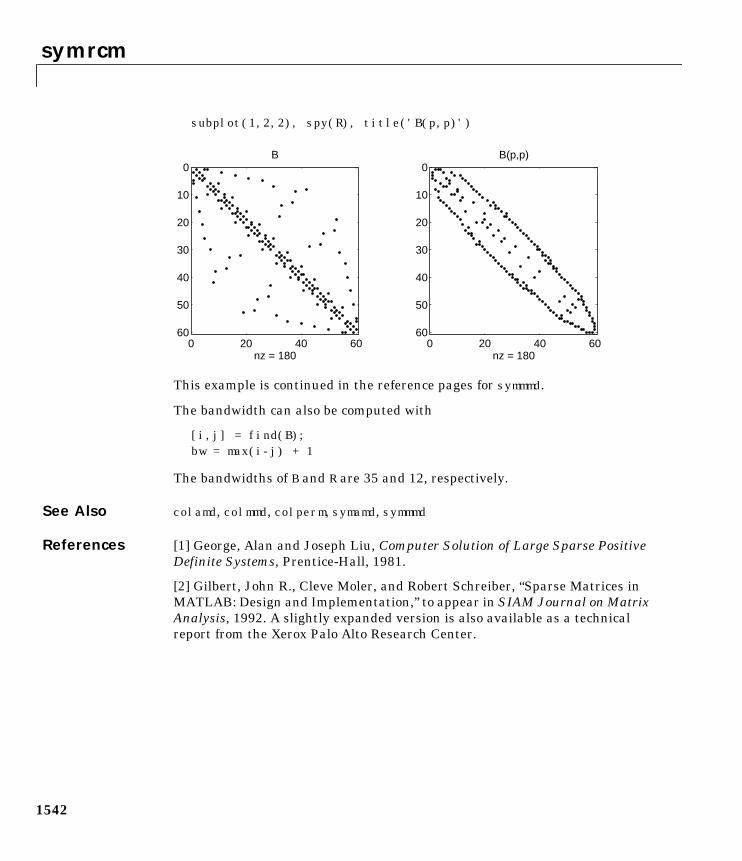
symrcm
1542
subplot(1,2,2), spy(R), title('B(p,p)')
This example is continued in the reference pages for symmmd.
The bandwidth can also be computed with
[i,j] = find(B);bw = max(i-j) + 1
The bandwidths of B and R are 35 and 12, respectively.
See Also colamd, colmmd, colperm, symamd, symmmd
References [1] George, Alan and Joseph Liu, Computer Solution of Large Sparse PositiveDefinite Systems, Prentice-Hall, 1981.
[2] Gilbert, John R., Cleve Moler, and Robert Schreiber, “Sparse Matrices inMATLAB: Design and Implementation,” to appear in SIAM Journal on MatrixAnalysis, 1992. A slightly expanded version is also available as a technicalreport from the Xerox Palo Alto Research Center.
0 20 40 60
0
10
20
30
40
50
60
nz = 180
B
0 20 40 60
0
10
20
30
40
50
60
nz = 180
B(p,p)
symvar
1543
1symvarPurpose Determine the symbolic variables in an expression
Syntax symvar 'expr's = symvar('expr')
Description symvar 'expr' searches the expression, expr, for identifiers other than i, j,pi, inf, nan, eps, and common functions. symvar displays those variables thatit finds or, if no such variable exists, displays an empty cell array, .
s = symvar('expr') returns the variables in a cell array of strings, s. If nosuch variable exists, s is an empty cell array.
Examples symvar finds variables beta1 and x, but skips pi and the cos function.
symvar 'cos(pi*x - beta1)'
ans =
'beta1' 'x'
See Also findstr
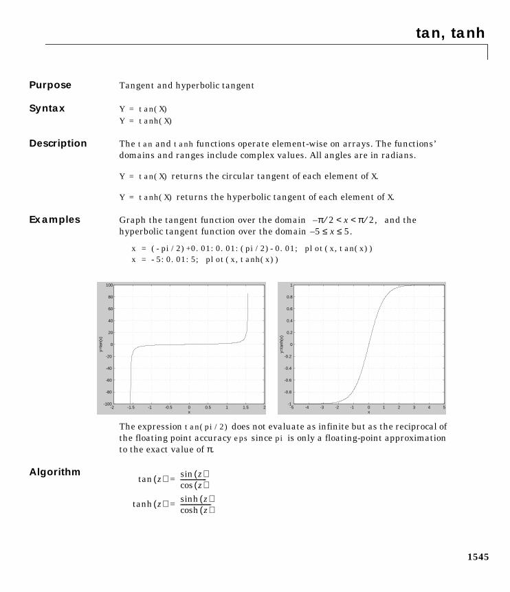
tan, tanh
1545
1tan, tanhPurpose Tangent and hyperbolic tangent
Syntax Y = tan(X)Y = tanh(X)
Description The tan and tanh functions operate element-wise on arrays. The functions’domains and ranges include complex values. All angles are in radians.
Y = tan(X) returns the circular tangent of each element of X.
Y = tanh(X) returns the hyperbolic tangent of each element of X.
Examples Graph the tangent function over the domain and thehyperbolic tangent function over the domain
x = (-pi/2)+0.01:0.01:(pi/2)-0.01; plot(x,tan(x))x = -5:0.01:5; plot(x,tanh(x))
The expression tan(pi/2) does not evaluate as infinite but as the reciprocal ofthe floating point accuracy eps since pi is only a floating-point approximationto the exact value of π.
Algorithm
π 2⁄– x π 2⁄ ,< <5– x 5.≤ ≤
-2 -1.5 -1 -0.5 0 0.5 1 1.5 2-100
-80
-60
-40
-20
0
20
40
60
80
100
x
y=ta
n(x)
-5 -4 -3 -2 -1 0 1 2 3 4 5-1
-0.8
-0.6
-0.4
-0.2
0
0.2
0.4
0.6
0.8
1
x
y=ta
nh(x
)
z( )tan z( )sinz( )cos
-----------------=
z( )tanh z( )sinhz( )cosh
--------------------=

tan, tanh
1546
See Also atan, atan2
tempdir
1547
1tempdirPurpose Return the name of the system’s temporary directory
Syntax tmp_dir = tempdir
Description tmp_dir = tempdir returns the name of the system’s temporary directory, ifone exists. This function does not create a new directory.
See Opening Temporary Files and Directories for more information.
See Also tempname
tempname
1548
1tempnamePurpose Unique name for temporary file
Syntax tmp_nam = tempname
Description tmp_nam = tempname returns a unique string, tmp_nam, suitable for use as atemporary filename.
See Opening Temporary Files and Directories for more information.
See Also tempdir
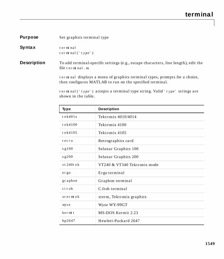
terminal
1549
1terminalPurpose Set graphics terminal type
Syntax terminalterminal('type')
Description To add terminal-specific settings (e.g., escape characters, line length), edit thefile terminal.m.
terminal displays a menu of graphics terminal types, prompts for a choice,then configures MATLAB to run on the specified terminal.
terminal('type') accepts a terminal type string. Valid 'type' strings areshown in the table.
Type Description
tek401x Tektronix 4010/4014
tek4100 Tektronix 4100
tek4105 Tektronix 4105
retro Retrographics card
sg100 Selanar Graphics 100
sg200 Selanar Graphics 200
vt240tek VT240 & VT340 Tektronix mode
ergo Ergo terminal
graphon Graphon terminal
citoh C.Itoh terminal
xtermtek xterm, Tektronix graphics
wyse Wyse WY-99GT
kermit MS-DOS Kermit 2.23
hp2647 Hewlett-Packard 2647
terminal
1550
hds Human Designed Systems
Type Description (Continued)
texlabel
1551
1texlabelPurpose Produce TeX format from character string
Syntax texlabel(f)texlabel(f,'literal')
Description texlabel(f) converts the MATLAB expression f into the TeX equivalent foruse in text strings. It processes Greek variable names (e.g., lambda, delta, etc.)into a string that displays as actual Greek letters.
texlabel(f,'literal') prints Greek variable names as literals.
If the string is too long to fit into a figure window, then the center of theexpression is replaced with a tilde ellipsis (~~~).
Examples You can use texlabel as an argument to the title, xlabel, ylabel, zlabel,and text commands. For example,
title(texlabel('sin(sqrt(x^2 + y^2))/sqrt(x^2 + y^2)'))
By default, texlabel translates Greek variable names to the equivalent Greekletter. You can select literal interpretation by including the literal argument.For example, compare these two commands.
text(.5,.5,...texlabel('lambda12^(3/2)/pi - pi*delta^(2/3)'))
text(.25,.25,...texlabel('lambda12^(3/2)/pi - pi*delta^(2/3)','literal'))
texlabel
1552
See Also text, title, xlabel, ylabel, zlabel, the text String property
0 0.1 0.2 0.3 0.4 0.5 0.6 0.7 0.8 0.9 10
0.1
0.2
0.3
0.4
0.5
0.6
0.7
0.8
0.9
1
λ12
3/2/π − π δ2/3
lambda123/2/pi − pi delta2/3
text
1553
1textPurpose Create text object in current axes
Syntax text(x,y,'string')text(x,y,z,'string')text(...'PropertyName',PropertyValue...)h = text(...)
Description text is the low-level function for creating text graphics objects. Use text toplace character strings at specified locations.
text(x,y,'string') adds the string in quotes to the location specified by thepoint (x,y).
text(x,y,z,'string') adds the string in 3-D coordinates.
text(x,y,z,'string','PropertyName',PropertyValue....) adds the stringin quotes to location defined by the coordinates and uses the values for thespecified text properties. See the text property list section at the end of thispage for a list of text properties.
text('PropertyName',PropertyValue....) omits the coordinates entirelyand specifies all properties using property name/property value pairs.
h = text(..) returns a column vector of handles to text objects, one handleper object. All forms of the text function optionally return this outputargument.
See the String property for a list of symbols, including Greek letters.
Remarks Specify the text location coordinates (the x, y, and z arguments) in the dataunits of the current axes (see “Examples”). The Extent, VerticalAlignment,and HorizontalAlignment properties control the positioning of the characterstring with regard to the text location point.
If the coordinates are vectors, text writes the string at all locations defined bythe list of points. If the character string is an array the same length as x, y, andz, text writes the corresponding row of the string array at each point specified.
When specifying strings for multiple text objects, the string can be
text
1554
• a cell array of strings
• a padded string matrix
• a string vector using vertical slash characters (‘|’) as separators.
Each element of the specified string array creates a different text object.
When specifying the string for a single text object, cell arrays of strings andpadded string matrices result in a text object with a multiline string, whilevertical slash characters are not interpreted as separators and result in asingle line string containing vertical slashes.
text is a low-level function that accepts property name/property value pairs asinput arguments, however; the convenience form,
text(x,y,z,'string')
is equivalent to:
text('XData',x,'YData',y,'ZData',z,'String','string')
You can specify other properties only as property name/property value pairs.See the text property list at the end of this page for a description of eachproperty. You can specify properties as property name/property value pairs,structure arrays, and cell arrays (see the set and get reference pages forexamples of how to specify these data types).
text does not respect the setting of the figure or axes NextPlot property. Thisallows you to add text objects to an existing axes without setting hold to on.
Examples The statements,
plot(0:pi/20:2*pi,sin(0:pi/20:2*pi))text(pi,0,' \leftarrow sin(\pi)','FontSize',18)
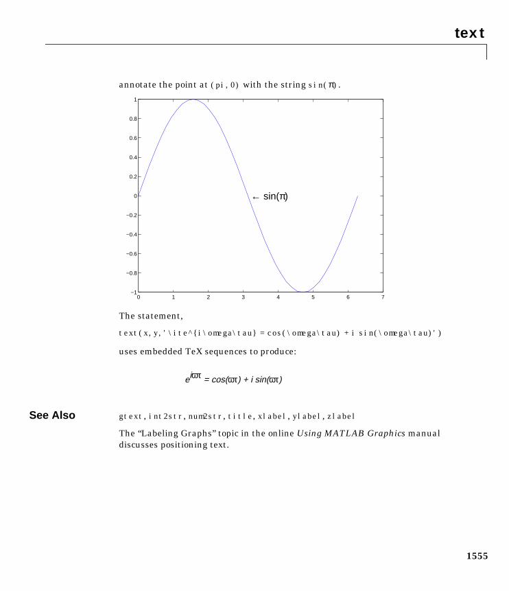
text
1555
annotate the point at (pi,0) with the string sin(π).
The statement,
text(x,y,'\ite^i\omega\tau = cos(\omega\tau) + i sin(\omega\tau)')
uses embedded TeX sequences to produce:
See Also gtext, int2str, num2str, title, xlabel, ylabel, zlabel
The “Labeling Graphs” topic in the online Using MATLAB Graphics manualdiscusses positioning text.
0 1 2 3 4 5 6 7−1
−0.8
−0.6
−0.4
−0.2
0
0.2
0.4
0.6
0.8
1
← sin(π)
eiωτ = cos(ωτ) + i sin(ωτ)
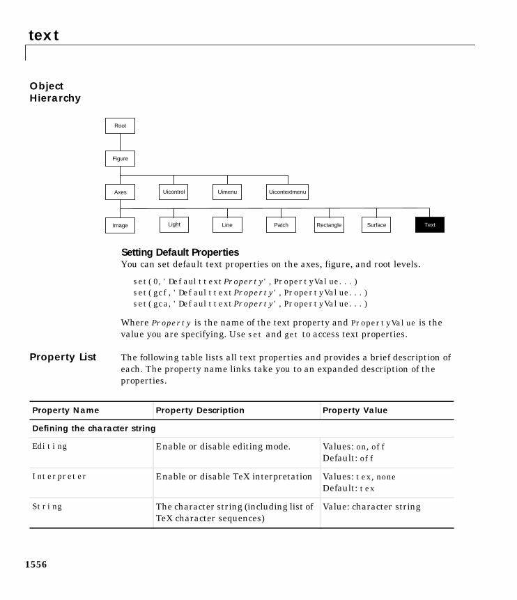
text
1556
ObjectHierarchy
Setting Default PropertiesYou can set default text properties on the axes, figure, and root levels.
set(0,'DefaulttextProperty',PropertyValue...)set(gcf,'DefaulttextProperty',PropertyValue...)set(gca,'DefaulttextProperty',PropertyValue...)
Where Property is the name of the text property and PropertyValue is thevalue you are specifying. Use set and get to access text properties.
Property List The following table lists all text properties and provides a brief description ofeach. The property name links take you to an expanded description of theproperties.
Uimenu
Line
Axes Uicontrol
Image
Figure
Uicontextmenu
Light SurfacePatch Text
Root
Rectangle
Property Name Property Description Property Value
Defining the character string
Editing Enable or disable editing mode. Values: on, offDefault: off
Interpreter Enable or disable TeX interpretation Values: tex, noneDefault: tex
String The character string (including list ofTeX character sequences)
Value: character string
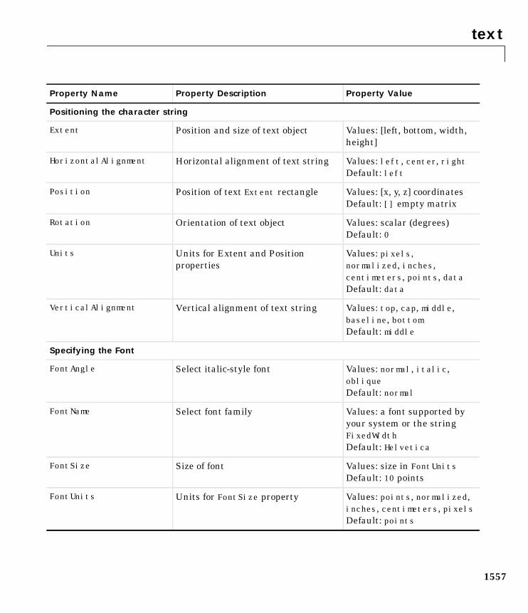
text
1557
Positioning the character string
Extent Position and size of text object Values: [left, bottom, width,height]
HorizontalAlignment Horizontal alignment of text string Values: left, center, rightDefault: left
Position Position of text Extent rectangle Values: [x, y, z] coordinatesDefault: [] empty matrix
Rotation Orientation of text object Values: scalar (degrees)Default: 0
Units Units for Extent and Positionproperties
Values: pixels,normalized, inches,centimeters, points, dataDefault: data
VerticalAlignment Vertical alignment of text string Values: top, cap, middle,baseline, bottomDefault: middle
Specifying the Font
FontAngle Select italic-style font Values: normal, italic,obliqueDefault: normal
FontName Select font family Values: a font supported byyour system or the stringFixedWidthDefault: Helvetica
FontSize Size of font Values: size in FontUnitsDefault: 10 points
FontUnits Units for FontSize property Values: points, normalized,inches, centimeters, pixelsDefault: points
Property Name Property Description Property Value
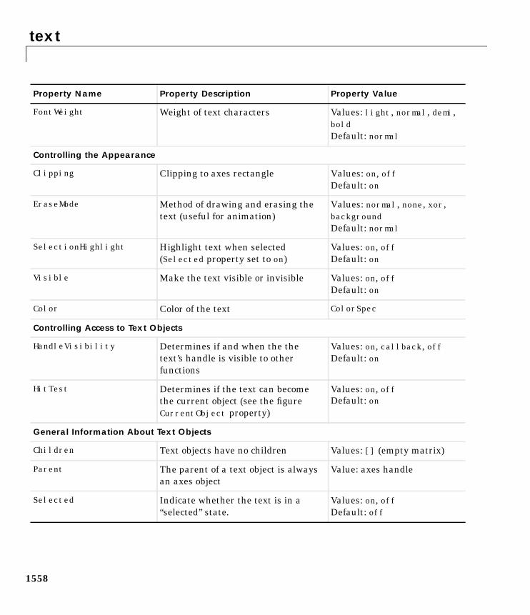
text
1558
FontWeight Weight of text characters Values: light, normal, demi,boldDefault: normal
Controlling the Appearance
Clipping Clipping to axes rectangle Values: on, offDefault: on
EraseMode Method of drawing and erasing thetext (useful for animation)
Values: normal, none, xor,backgroundDefault: normal
SelectionHighlight Highlight text when selected(Selected property set to on)
Values: on, offDefault: on
Visible Make the text visible or invisible Values: on, offDefault: on
Color Color of the text ColorSpec
Controlling Access to Text Objects
HandleVisibility Determines if and when the thetext’s handle is visible to otherfunctions
Values: on, callback, offDefault: on
HitTest Determines if the text can becomethe current object (see the figureCurrentObject property)
Values: on, offDefault: on
General Information About Text Objects
Children Text objects have no children Values: [] (empty matrix)
Parent The parent of a text object is alwaysan axes object
Value: axes handle
Selected Indicate whether the text is in a“selected” state.
Values: on, offDefault: off
Property Name Property Description Property Value
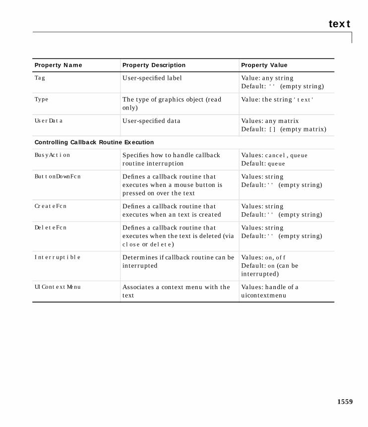
text
1559
Tag User-specified label Value: any stringDefault: '' (empty string)
Type The type of graphics object (readonly)
Value: the string 'text'
UserData User-specified data Values: any matrixDefault: [] (empty matrix)
Controlling Callback Routine Execution
BusyAction Specifies how to handle callbackroutine interruption
Values: cancel, queueDefault: queue
ButtonDownFcn Defines a callback routine thatexecutes when a mouse button ispressed on over the text
Values: stringDefault: '' (empty string)
CreateFcn Defines a callback routine thatexecutes when an text is created
Values: stringDefault: '' (empty string)
DeleteFcn Defines a callback routine thatexecutes when the text is deleted (viaclose or delete)
Values: stringDefault: '' (empty string)
Interruptible Determines if callback routine can beinterrupted
Values: on, offDefault: on (can beinterrupted)
UIContextMenu Associates a context menu with thetext
Values: handle of auicontextmenu
Property Name Property Description Property Value
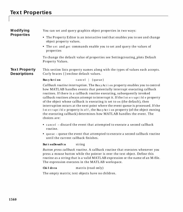
Text Properties
1560
1Text PropertiesModifyingProperties
You can set and query graphics object properties in two ways:
• The Property Editor is an interactive tool that enables you to see and changeobject property values.
• The set and get commands enable you to set and query the values ofproperties
To change the default value of properties see Settingcreating_plots DefaultProperty Values.
Text PropertyDescriptions
This section lists property names along with the types of values each accepts.Curly braces enclose default values.
BusyAction cancel | queue
Callback routine interruption. The BusyAction property enables you to controlhow MATLAB handles events that potentially interrupt executing callbackroutines. If there is a callback routine executing, subsequently invokedcallback routines always attempt to interrupt it. If the Interruptible propertyof the object whose callback is executing is set to on (the default), theninterruption occurs at the next point where the event queue is processed. If theInterruptible property is off, the BusyAction property (of the object owningthe executing callback) determines how MATLAB handles the event. Thechoices are:
• cancel – discard the event that attempted to execute a second callbackroutine.
• queue – queue the event that attempted to execute a second callback routineuntil the current callback finishes.
ButtonDownFcn string
Button press callback routine. A callback routine that executes whenever youpress a mouse button while the pointer is over the text object. Define thisroutine as a string that is a valid MATLAB expression or the name of an M-file.The expression executes in the MATLAB workspace.
Children matrix (read only)
The empty matrix; text objects have no children.
Text Properties
1561
Clipping on | off
Clipping mode. When Clipping is on, MATLAB does not display any portionof the text that is outside the axes.
Color ColorSpec
Text color. A three-element RGB vector or one of MATLAB ’s predefined names,specifying the text color. The default value for Color is white. See ColorSpecfor more information on specifying color.
CreateFcn string
Callback routine executed during object creation. This property defines acallback routine that executes when MATLAB creates a text object. You mustdefine this property as a default value for text. For example, the statement,
set(0,'DefaultTextCreateFcn',...'set(gcf,''Pointer'',’'crosshair'')')
defines a default value on the root level that sets the figure Pointer propertyto a crosshair whenever you create a text object. MATLAB executes this routineafter setting all text properties. Setting this property on an existing text objecthas no effect.
The handle of the object whose CreateFcn is being executed is accessible onlythrough the root CallbackObject property, which you can query using gcbo.
DeleteFcn string
Delete text callback routine. A callback routine that executes when you deletethe text object (e.g., when you issue a delete command or clear the axes orfigure). MATLAB executes the routine before destroying the object’s propertiesso these values are available to the callback routine.
The handle of the object whose DeleteFcn is being executed is accessible onlythrough the root CallbackObject property, which you can query using gcbo.
Editing on | off
Enable or disable editing mode. When this property is set to the default off,you cannot edit the text string interactively (i.e., you must change the Stringproperty to change the text). When this property is set to on, MATLAB placesan insert cursor at the beginning of the text string and enables editing. Toapply the new text string:
Text Properties
1562
• Press the ESC key
• Clicking in any figure window (including the current figure)
• Reset the Editing property to off
MATLAB then updates the String property to contain the new text and resetsthe Editing property to off. You must reset the Editing property to on toagain resume editing.
EraseMode normal | none | xor | background
Erase mode. This property controls the technique MATLAB uses to draw anderase text objects. Alternative erase modes are useful for creating animatedsequences, where controlling the way individual object redraw is necessary toimprove performance and obtain the desired effect.
• normal — Redraw the affected region of the display, performing thethree-dimensional analysis necessary to ensure that all objects are renderedcorrectly. This mode produces the most accurate picture, but is the slowest.The other modes are faster, but do not perform a complete redraw and aretherefore less accurate.
• none — Do not erase the text when it is moved or destroyed. While the objectis still visible on the screen after erasing with EraseMode none, you cannotprint it because MATLAB stores no information about its former location.
• xor — Draw and erase the text by performing an exclusive OR (XOR) witheach pixel index of the screen beneath it. When the text is erased, it does notdamage the objects beneath it. However, when text is drawn in xor mode, itscolor depends on the color of the screen beneath it and is correctly coloredonly when over axes background Color, or the figure background Color if theaxes Color is set to none.
• background — Erase the text by drawing it in the background Color, or thefigure background Color if the axes Color is set to none. This damagesobjects that are behind the erased text, but text is always properly colored.
Printing with Non-normal Erase Modes. MATLAB always prints figures as if theEraseMode of all objects is normal. This means graphics objects created withEraseMode set to none, xor, or background can look different on screen than onpaper. On screen, MATLAB may mathematically combine layers of colors (e.g.,XORing a pixel color with that of the pixel behind it) and ignore
Text Properties
1563
three-dimensional sorting to obtain greater rendering speed. However, thesetechniques are not applied to the printed output.
You can use the MATLAB getframe command or other screen captureapplication to create an image of a figure containing non-normal mode objects.
Extent position rectangle (read only)
Position and size of text. A four-element read-only vector that defines the sizeand position of the text string.
[left,bottom,width,height]
If the Units property is set to data (the default), left and bottom are the x andy coordinates of the lower-left corner of the text Extent rectangle.
For all other values of Units, left and bottom are the distance from thelower-left corner of the axes position rectangle to the lower-left corner of thetext Extent rectangle. width and height are the dimensions of the Extentrectangle. All measurements are in units specified by the Units property.
FontAngle normal | italic | oblique
Character slant. MATLAB uses this property to select a font from thoseavailable on your particular system. Generally, setting this property to italicor oblique selects a slanted font.
FontName A name such as Courier or the string FixedWidth
Font family. A string specifying the name of the font to use for the text object.To display and print properly, this must be a font that your system supports.The default font is Helvetica.
Specifying a Fixed-Width FontIf you want text to use a fixed-width font that looks good in any locale, youshould set FontName to the string FixedWidth:
set(text_handle,'FontName','FixedWidth')
This eliminates the need to hardcode the name of a fixed-width font, which maynot display text properly on systems that do not use ASCII character encoding(such as in Japan where multibyte character sets are used). A properly writtenMATLAB application that needs to use a fixed-width font should set FontName
Text Properties
1564
to FixedWidth (note that this string is case sensitive) and rely onFixedWidthFontName to be set correctly in the end-user’s environment.
End users can adapt a MATLAB application to different locales or personalenvironments by setting the root FixedWidthFontName property to theappropriate value for that locale from startup.m.
Note that setting the root FixedWidthFontName property causes an immediateupdate of the display to use the new font.
FontSize size in FontUnits
Font size. An integer specifying the font size to use for text, in units determinedby the FontUnits property. The default point size is 10 (1 point = 1/72 inch).
FontWeight light | normal | demi | bold
Weight of text characters. MATLAB uses this property to select a font fromthose available on your particular system. Generally, setting this property tobold or demi causes MATLAB to use a bold font.
FontUnits points | normalized | inches |centimeters | pixels
Font size units. MATLAB uses this property to determine the units used by theFontSize property. Normalized units interpret FontSize as a fraction of theheight of the parent axes. When you resize the axes, MATLAB modifies thescreen FontSize accordingly. pixels, inches, centimeters, and points areabsolute units (1 point = 1/72 inch).
HandleVisibility on | callback | off
Control access to object’s handle by command-line users and GUIs. Thisproperty determines when an object’s handle is visible in its parent’s list ofchildren. HandleVisibility is useful for preventing command-line users fromaccidentally drawing into or deleting a figure that contains only user interfacedevices (such as a dialog box).
Handles are always visible when HandleVisibility is on.
Setting HandleVisibility to callback causes handles to be visible fromwithin callback routines or functions invoked by callback routines, but not fromwithin functions invoked from the command line. This provides a means toprotect GUIs from command-line users, while allowing callback routines tohave complete access to object handles.
Text Properties
1565
Setting HandleVisibility to off makes handles invisible at all times. Thismay be necessary when a callback routine invokes a function that mightpotentially damage the GUI (such as evaluating a user-typed string), and sotemporarily hides its own handles during the execution of that function.
When a handle is not visible in its parent’s list of children, it cannot be returnedby functions that obtain handles by searching the object hierarchy or queryinghandle properties. This includes get, findobj, gca, gcf, gco, newplot, cla, clf,and close.
When a handle’s visibility is restricted using callback or off, the object’shandle does not appear in its parent’s Children property, figures do not appearin the root’s CurrentFigure property, objects do not appear in the root’sCallbackObject property or in the figure’s CurrentObject property, and axesdo not appear in their parent’s CurrentAxes property.
You can set the root ShowHiddenHandles property to on to make all handlesvisible, regardless of their HandleVisibility settings (this does not affect thevalues of the HandleVisibility properties).
Handles that are hidden are still valid. If you know an object’s handle, you canset and get its properties, and pass it to any function that operates on handles.
HitTest on | off
Selectable by mouse click. HitTest determines if the text can become thecurrent object (as returned by the gco command and the figure CurrentObjectproperty) as a result of a mouse click on the text. If HitTest is off, clicking onthe text selects the object below it (which is usually the axes containing it).
For example, suppose you define the button down function of an image (see theButtonDownFcn property) to display text at the location you click on with themouse.
First define the callback routine.
function bd_functionpt = get(gca,'CurrentPoint');text(pt(1,1),pt(1,2),pt(1,3),...
'\fontsize20\oplus The spot to label',...'HitTest','off')
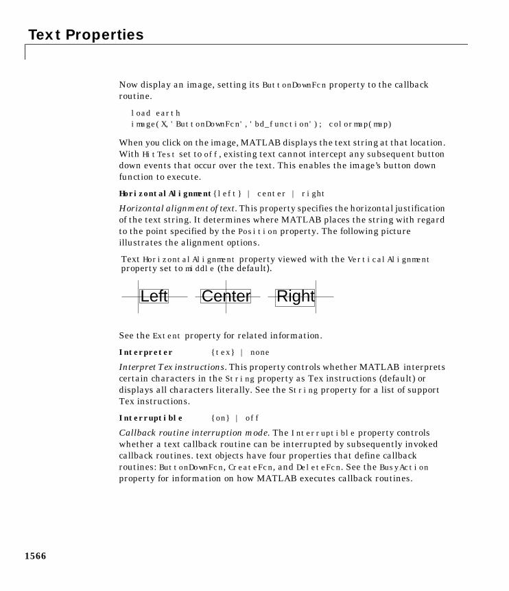
Text Properties
1566
Now display an image, setting its ButtonDownFcn property to the callbackroutine.
load earthimage(X,'ButtonDownFcn','bd_function'); colormap(map)
When you click on the image, MATLAB displays the text string at that location.With HitTest set to off, existing text cannot intercept any subsequent buttondown events that occur over the text. This enables the image’s button downfunction to execute.
HorizontalAlignmentleft | center | right
Horizontal alignment of text. This property specifies the horizontal justificationof the text string. It determines where MATLAB places the string with regardto the point specified by the Position property. The following pictureillustrates the alignment options.
See the Extent property for related information.
Interpreter tex | none
Interpret Tex instructions. This property controls whether MATLAB interpretscertain characters in the String property as Tex instructions (default) ordisplays all characters literally. See the String property for a list of supportTex instructions.
Interruptible on | off
Callback routine interruption mode. The Interruptible property controlswhether a text callback routine can be interrupted by subsequently invokedcallback routines. text objects have four properties that define callbackroutines: ButtonDownFcn, CreateFcn, and DeleteFcn. See the BusyActionproperty for information on how MATLAB executes callback routines.
Left Center Right
Text HorizontalAlignment property viewed with the VerticalAlignmentproperty set to middle (the default).
Text Properties
1567
Parent handle
Text object’s parent. The handle of the text object’s parent object. The parent ofa text object is the axes in which it is displayed. You can move a text object toanother axes by setting this property to the handle of the new parent.
Position [x,y,[z]]
Location of text. A two- or three-element vector, [x y [z]], that specifies thelocation of the text in three dimensions. If you omit the z value, it defaults to0. All measurements are in units specified by the Units property. Initial valueis [0 0 0].
Rotation scalar (default = 0)
Text orientation. This property determines the orientation of the text string.Specify values of rotation in degrees (positive angles cause counterclockwiserotation).
Selected on | off
Is object selected? When this property is on, MATLAB displays selectionhandles if the SelectionHighlight property is also on. You can, for example,define the ButtonDownFcn to set this property, allowing users to select theobject with the mouse.
SelectionHighlight on | off
Objects highlight when selected. When the Selected property is on, MATLABindicates the selected state by drawing four edge handles and four cornerhandles. When SelectionHighlight is off, MATLAB does not draw thehandles.
String string
The text string. Specify this property as a quoted string for single-line strings,or as a cell array of strings or a padded string matrix for multiline strings.MATLAB displays this string at the specified location. Vertical slashcharacters are not interpreted as linebreaks in text strings, and are drawn aspart of the text string. See the “Remarks” section for more information.
When the text Interpreter property is Tex (the default), you can use a subsetof TeX commands embedded in the string to produce special characters such as
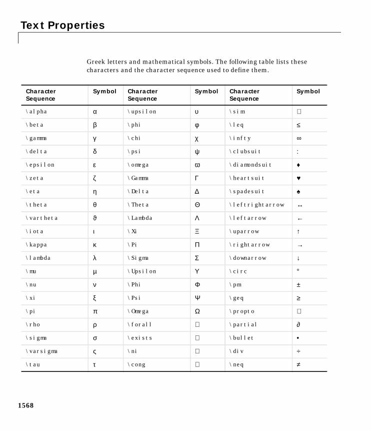
Text Properties
1568
Greek letters and mathematical symbols. The following table lists thesecharacters and the character sequence used to define them.
CharacterSequence
Symbol CharacterSequence
Symbol CharacterSequence
Symbol
\alpha α \upsilon υ \sim ∼
\beta β \phi φ \leq ≤
\gamma γ \chi χ \infty ∞
\delta δ \psi ψ \clubsuit ♣
\epsilon ε \omega ω \diamondsuit ♦
\zeta ζ \Gamma Γ \heartsuit ♥
\eta η \Delta ∆ \spadesuit ♠
\theta θ \Theta Θ \leftrightarrow ↔
\vartheta ϑ \Lambda Λ \leftarrow ←
\iota ι \Xi Ξ \uparrow ↑
\kappa κ \Pi Π \rightarrow →
\lambda λ \Sigma Σ \downarrow ↓
\mu µ \Upsilon Υ \circ °
\nu ν \Phi Φ \pm ±
\xi ξ \Psi Ψ \geq ≥
\pi π \Omega Ω \propto ∝
\rho ρ \forall ∀ \partial ∂
\sigma σ \exists ∃ \bullet •
\varsigma ς \ni ∋ \div ÷
\tau τ \cong ≅ \neq ≠
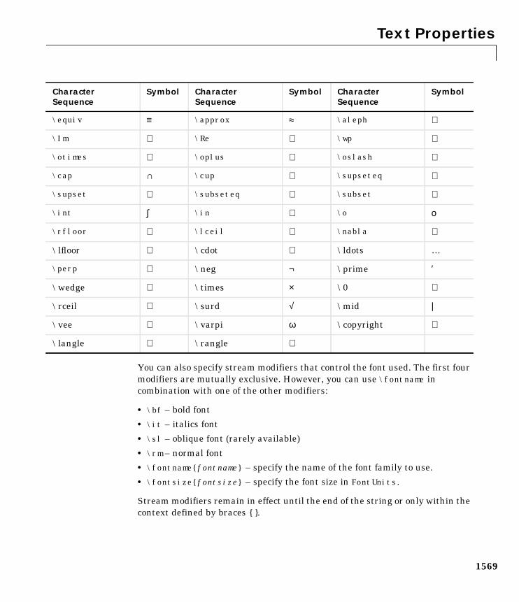
Text Properties
1569
You can also specify stream modifiers that control the font used. The first fourmodifiers are mutually exclusive. However, you can use \fontname incombination with one of the other modifiers:
• \bf – bold font
• \it – italics font
• \sl – oblique font (rarely available)
• \rm – normal font
• \fontnamefontname – specify the name of the font family to use.
• \fontsizefontsize – specify the font size in FontUnits.
Stream modifiers remain in effect until the end of the string or only within thecontext defined by braces .
\equiv ≡ \approx ≈ \aleph ℵ
\Im ℑ \Re ℜ \wp ℘
\otimes ⊗ \oplus ⊕ \oslash ∅
\cap ∩ \cup ∪ \supseteq ⊇
\supset ⊃ \subseteq ⊆ \subset ⊂
\int ∫ \in ∈ \o ο
\rfloor \lceil \nabla ∇
\lfloor \cdot ⋅ \ldots …
\perp ⊥ \neg ¬ \prime ′
\wedge ∧ \times × \0 ∅
\rceil \surd √ \mid |
\vee ∨ \varpi ϖ \copyright
\langle ⟨ \rangle ⟩
CharacterSequence
Symbol CharacterSequence
Symbol CharacterSequence
Symbol
Text Properties
1570
Specifying Subscript and Superscript CharactersThe subscript character “_” and the superscript character “^” modify thecharacter or substring defined in braces immediately following.
To print the special characters used to define the Tex strings whenInterpreter is Tex, prefix them with the backslash “\” character: \\, \, \ \_,\^.
See the example for more information.
When Interpreter is none, no characters in the String are interpreted, andall are displayed when the text is drawn.
Tag string
User-specified object label. The Tag property provides a means to identifygraphics objects with a user-specified label. This is particularly useful whenconstructing interactive graphics programs that would otherwise need todefine object handles as global variables or pass them as arguments betweencallback routines. You can define Tag as any string.
Type string (read only)
Class of graphics object. For text objects, Type is always the string 'text'.
Units pixels | normalized | inches |centimeters | points | data
Units of measurement. This property specifies the units MATLAB uses tointerpret the Extent and Position properties. All units are measured from thelower-left corner of the axes plotbox. Normalized units map the lower-leftcorner of the rectangle defined by the axes to (0,0) and the upper-right cornerto (1.0,1.0). pixels, inches, centimeters, and points are absolute units (1point = 1/72 inch). data refers to the data units of the parent axes.
If you change the value of Units, it is good practice to return it to its defaultvalue after completing your computation so as not to affect other functions thatassume Units is set to the default value.
UserData matrix
User-specified data. Any data you want to associate with the text object.MATLAB does not use this data, but you can access it using set and get.
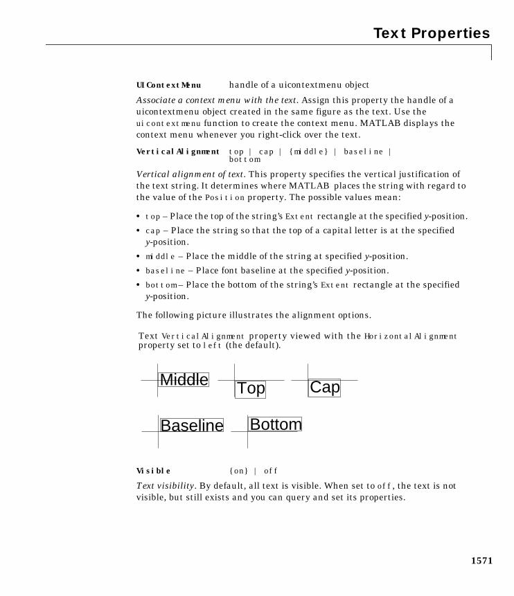
Text Properties
1571
UIContextMenu handle of a uicontextmenu object
Associate a context menu with the text. Assign this property the handle of auicontextmenu object created in the same figure as the text. Use theuicontextmenu function to create the context menu. MATLAB displays thecontext menu whenever you right-click over the text.
VerticalAlignment top | cap | middle | baseline |bottom
Vertical alignment of text. This property specifies the vertical justification ofthe text string. It determines where MATLAB places the string with regard tothe value of the Position property. The possible values mean:
• top – Place the top of the string’s Extent rectangle at the specified y-position.
• cap – Place the string so that the top of a capital letter is at the specifiedy-position.
• middle – Place the middle of the string at specified y-position.
• baseline – Place font baseline at the specified y-position.
• bottom – Place the bottom of the string’s Extent rectangle at the specifiedy-position.
The following picture illustrates the alignment options.
Visible on | off
Text visibility. By default, all text is visible. When set to off, the text is notvisible, but still exists and you can query and set its properties.
Middle Top Cap
Baseline Bottom
Text VerticalAlignment property viewed with the HorizontalAlignmentproperty set to left (the default).
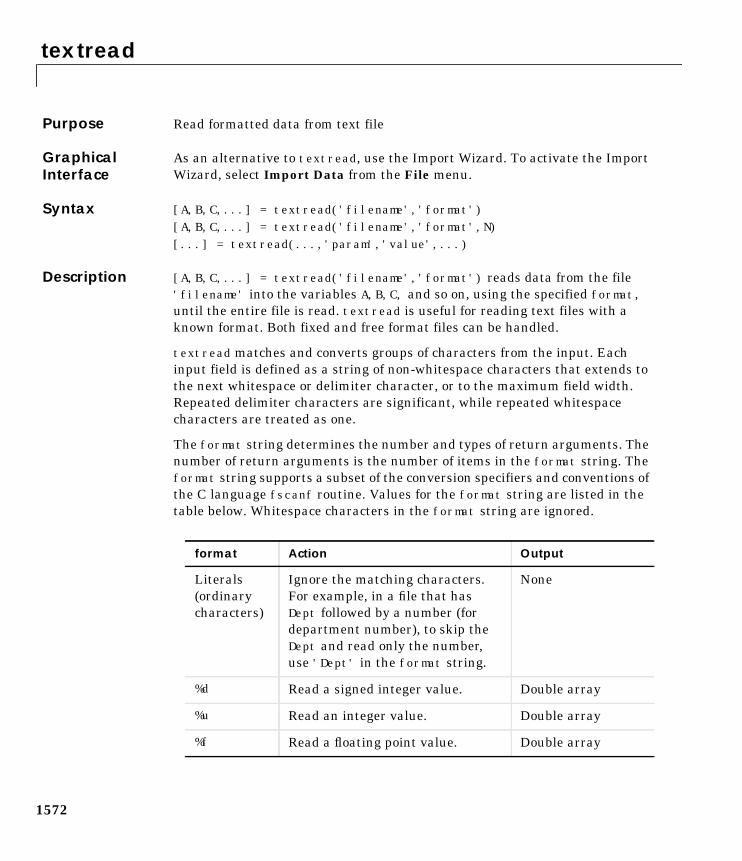
textread
1572
1textreadPurpose Read formatted data from text file
GraphicalInterface
As an alternative to textread, use the Import Wizard. To activate the ImportWizard, select Import Data from the File menu.
Syntax [A,B,C,...] = textread('filename','format')[A,B,C,...] = textread('filename','format',N)[...] = textread(...,'param','value',...)
Description [A,B,C,...] = textread('filename','format') reads data from the file'filename' into the variables A,B,C, and so on, using the specified format,until the entire file is read. textread is useful for reading text files with aknown format. Both fixed and free format files can be handled.
textread matches and converts groups of characters from the input. Eachinput field is defined as a string of non-whitespace characters that extends tothe next whitespace or delimiter character, or to the maximum field width.Repeated delimiter characters are significant, while repeated whitespacecharacters are treated as one.
The format string determines the number and types of return arguments. Thenumber of return arguments is the number of items in the format string. Theformat string supports a subset of the conversion specifiers and conventions ofthe C language fscanf routine. Values for the format string are listed in thetable below. Whitespace characters in the format string are ignored.
format Action Output
Literals(ordinarycharacters)
Ignore the matching characters.For example, in a file that hasDept followed by a number (fordepartment number), to skip theDept and read only the number,use 'Dept' in the format string.
None
%d Read a signed integer value. Double array
%u Read an integer value. Double array
%f Read a floating point value. Double array
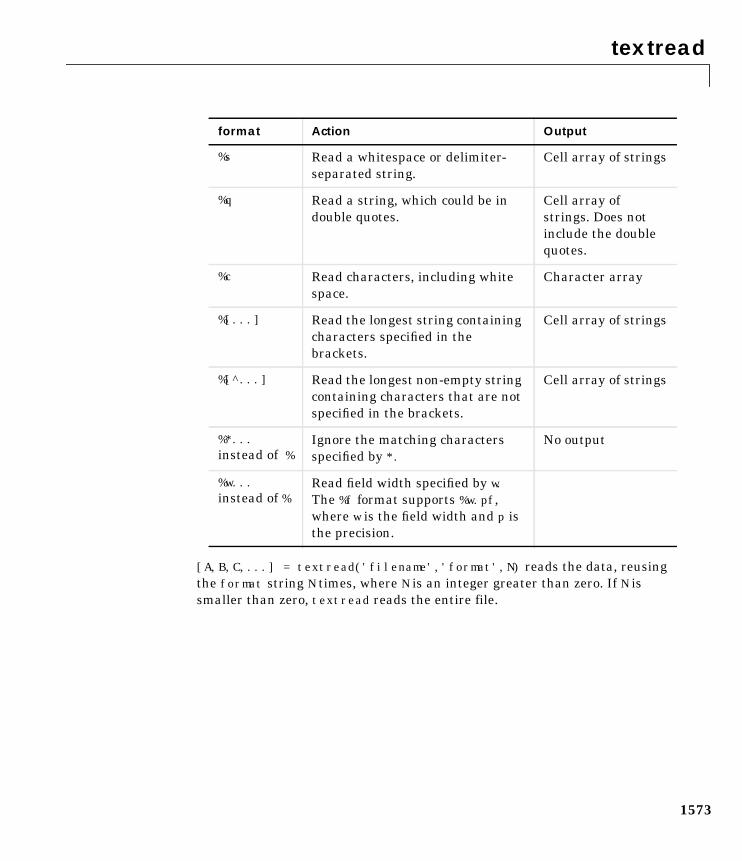
textread
1573
[A,B,C,...] = textread('filename','format',N) reads the data, reusingthe format string N times, where N is an integer greater than zero. If N issmaller than zero, textread reads the entire file.
%s Read a whitespace or delimiter-separated string.
Cell array of strings
%q Read a string, which could be indouble quotes.
Cell array ofstrings. Does notinclude the doublequotes.
%c Read characters, including whitespace.
Character array
%[...] Read the longest string containingcharacters specified in thebrackets.
Cell array of strings
%[^...] Read the longest non-empty stringcontaining characters that are notspecified in the brackets.
Cell array of strings
%*...instead of %
Ignore the matching charactersspecified by *.
No output
%w...instead of %
Read field width specified by w.The %f format supports %w.pf,where w is the field width and p isthe precision.
format Action Output
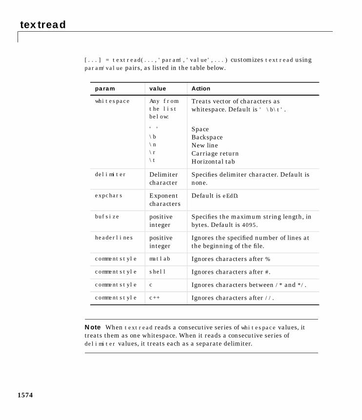
textread
1574
[...] = textread(...,'param','value',...) customizes textread usingparam/value pairs, as listed in the table below.
Note When textread reads a consecutive series of whitespace values, ittreats them as one whitespace. When it reads a consecutive series ofdelimiter values, it treats each as a separate delimiter.
param value Action
whitespace Any fromthe listbelow:
Treats vector of characters aswhitespace. Default is ' \b\t'.
' '\b\n\r\t
SpaceBackspaceNew lineCarriage returnHorizontal tab
delimiter Delimitercharacter
Specifies delimiter character. Default isnone.
expchars Exponentcharacters
Default is eEdD.
bufsize positiveinteger
Specifies the maximum string length, inbytes. Default is 4095.
headerlines positiveinteger
Ignores the specified number of lines atthe beginning of the file.
commentstyle matlab Ignores characters after %
commentstyle shell Ignores characters after #.
commentstyle c Ignores characters between /* and */.
commentstyle c++ Ignores characters after //.
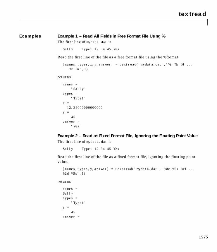
textread
1575
Examples Example 1 – Read All Fields in Free Format File Using %The first line of mydata.dat is
Sally Type1 12.34 45 Yes
Read the first line of the file as a free format file using the % format.
[names,types,x,y,answer] = textread('mydata.dat','%s %s %f ...%d %s',1)
returns
names = 'Sally'types = 'Type1'x = 12.34000000000000y = 45answer = 'Yes'
Example 2 – Read as Fixed Format File, Ignoring the Floating Point ValueThe first line of mydata.dat is
Sally Type1 12.34 45 Yes
Read the first line of the file as a fixed format file, ignoring the floating pointvalue.
[names,types,y,answer] = textread('mydata.dat','%9c %5s %*f ...%2d %3s',1)
returns
names =Sallytypes = 'Type1'y = 45answer =
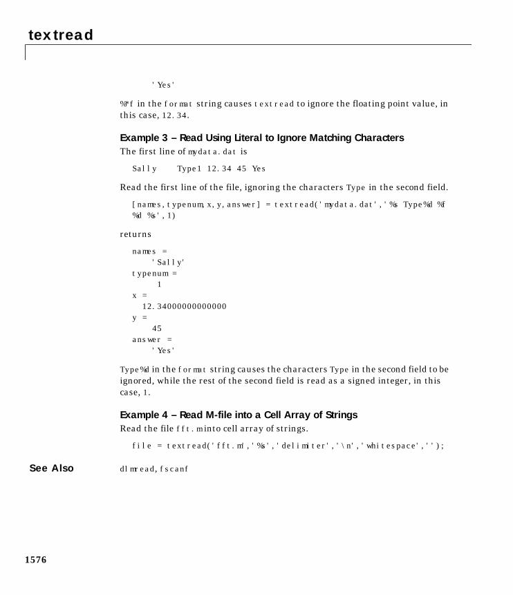
textread
1576
'Yes'
%*f in the format string causes textread to ignore the floating point value, inthis case, 12.34.
Example 3 – Read Using Literal to Ignore Matching CharactersThe first line of mydata.dat is
Sally Type1 12.34 45 Yes
Read the first line of the file, ignoring the characters Type in the second field.
[names,typenum,x,y,answer] = textread('mydata.dat','%s Type%d %f%d %s',1)
returns
names = 'Sally'typenum = 1x = 12.34000000000000y = 45answer = 'Yes'
Type%d in the format string causes the characters Type in the second field to beignored, while the rest of the second field is read as a signed integer, in thiscase, 1.
Example 4 – Read M-file into a Cell Array of StringsRead the file fft.m into cell array of strings.
file = textread('fft.m','%s','delimiter','\n','whitespace','');
See Also dlmread, fscanf
textwrap
1577
1textwrapPurpose Return wrapped string matrix for given uicontrol
Syntax outstring = textwrap(h,instring)[outstring,position] = textwrap(h,instring)
Description outstring = textwrap(h,instring) returns a wrapped string cell array,outstring, that fits inside the uicontrol with handle h. instring is a cell array,with each cell containing a single line of text. outstring is the wrapped stringmatrix in cell array format. Each cell of the input string is considered aparagraph.
[outstring,position]=textwrap(h,instring) returns the recommendedposition of the uicontrol in the units of the uicontrol. position considers theextent of the multiline text in the x and y directions.
Example Place a textwrapped string in a uicontrol:
pos = [10 10 100 10];h = uicontrol('Style','Text','Position',pos);string = 'This is a string for the uicontrol.',
'It should be correctly wrapped inside.';[outstring,newpos] = textwrap(h,string);pos(4) = newpos(4);set(h,'String',outstring,'Position',[pos(1),pos(2),pos(3)+10,pos(4)])
See Also uicontrol
tic, toc
1578
1tic, tocPurpose Stopwatch timer
Syntax ticany statements
toct = toc
Description tic starts a stopwatch timer.
toc prints the elapsed time since tic was used.
t = toc returns the elapsed time in t.
Examples This example measures how the time required to solve a linear system varieswith the order of a matrix.
for n = 1:100A = rand(n,n);b = rand(n,1);ticx = A\b;t(n) = toc;
endplot(t)
See Also clock, cputime, etime
title
1579
1titlePurpose Add title to current axes
Syntax title('string')title(fname)title(...,'PropertyName',PropertyValue,...)h = title(...)
Description Each axes graphics object can have one title. The title is located at the top andin the center of the axes.
title('string') outputs the string at the top and in the center of the currentaxes.
title(fname) evaluates the function that returns a string and displays thestring at the top and in the center of the current axes.
title(...,'PropertyName',PropertyValue,...) specifies property nameand property value pairs for the text graphics object that title creates.
h = title(...) returns the handle to the text object used as the title.
Examples Display today’s date in the current axes:
title(date)
Include a variable’s value in a title:
f = 70;c = (f—32)/1.8;title(['Temperature is ',num2str(c),'C'])
Include a variable’s value in a title and set the color of the title to yellow:
n = 3;title(['Case number #',int2str(n)],'Color','y')
Include Greek symbols in a title:
title('\ite^\omega\tau = cos(\omega\tau) + isin(\omega\tau)’)
Include a superscript character in a title:
title('\alpha^2’)
title
1580
Include a subscript character in a title:
title('X_1')
The text object String property lists the available symbols.
Remarks title sets the Title property of the current axes graphics object to a new textgraphics object. See the text String property for more information.
See Also gtext, int2str, num2str, plot, text, xlabel, ylabel, zlabel
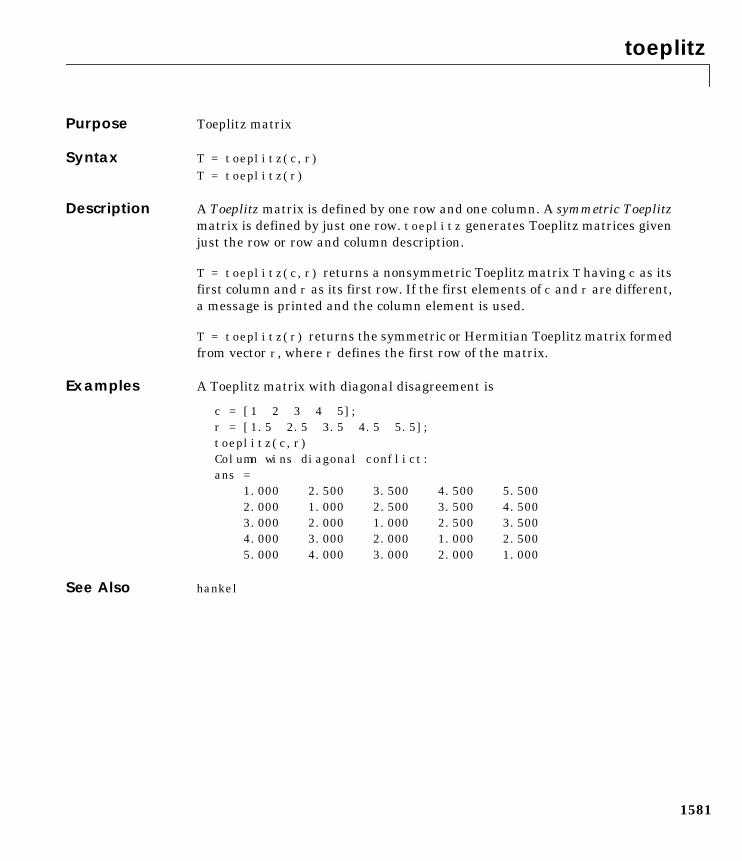
toeplitz
1581
1toeplitzPurpose Toeplitz matrix
Syntax T = toeplitz(c,r)T = toeplitz(r)
Description A Toeplitz matrix is defined by one row and one column. A symmetric Toeplitzmatrix is defined by just one row. toeplitz generates Toeplitz matrices givenjust the row or row and column description.
T = toeplitz(c,r) returns a nonsymmetric Toeplitz matrix T having c as itsfirst column and r as its first row. If the first elements of c and r are different,a message is printed and the column element is used.
T = toeplitz(r) returns the symmetric or Hermitian Toeplitz matrix formedfrom vector r, where r defines the first row of the matrix.
Examples A Toeplitz matrix with diagonal disagreement is
c = [1 2 3 4 5];r = [1.5 2.5 3.5 4.5 5.5];toeplitz(c,r)Column wins diagonal conflict:ans =
1.000 2.500 3.500 4.500 5.5002.000 1.000 2.500 3.500 4.5003.000 2.000 1.000 2.500 3.5004.000 3.000 2.000 1.000 2.5005.000 4.000 3.000 2.000 1.000
See Also hankel
trace
1582
1tracePurpose Sum of diagonal elements
Syntax b = trace(A)
Description b = trace(A) is the sum of the diagonal elements of the matrix A.
Algorithm trace is a single-statement M-file.
t = sum(diag(A));
See Also det, eig
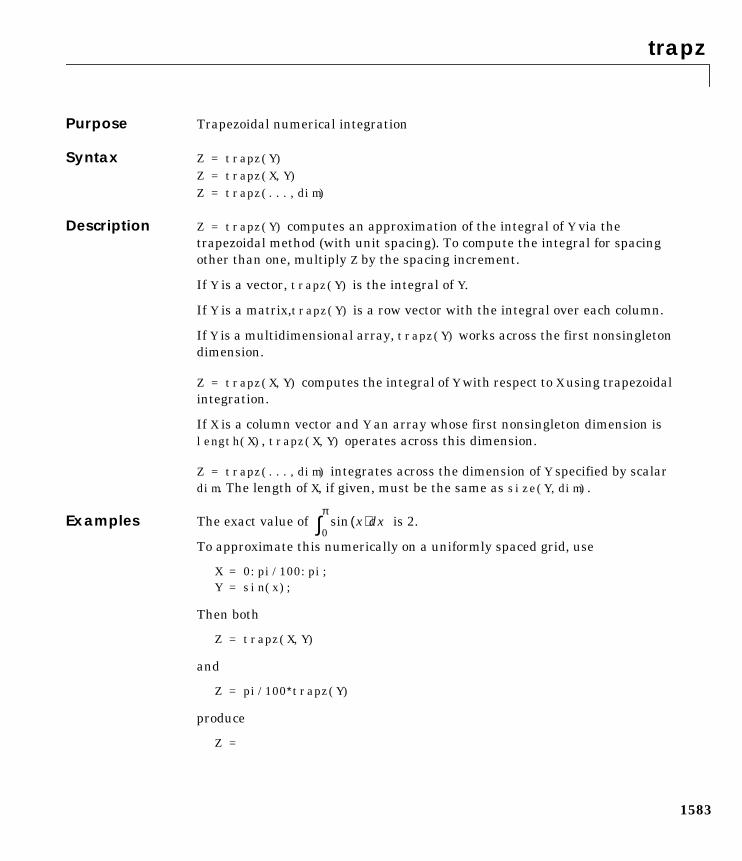
trapz
1583
1trapzPurpose Trapezoidal numerical integration
Syntax Z = trapz(Y)Z = trapz(X,Y)Z = trapz(...,dim)
Description Z = trapz(Y) computes an approximation of the integral of Y via thetrapezoidal method (with unit spacing). To compute the integral for spacingother than one, multiply Z by the spacing increment.
If Y is a vector, trapz(Y) is the integral of Y.
If Y is a matrix,trapz(Y) is a row vector with the integral over each column.
If Y is a multidimensional array, trapz(Y) works across the first nonsingletondimension.
Z = trapz(X,Y) computes the integral of Y with respect to X using trapezoidalintegration.
If X is a column vector and Y an array whose first nonsingleton dimension islength(X), trapz(X,Y) operates across this dimension.
Z = trapz(...,dim) integrates across the dimension of Y specified by scalardim. The length of X, if given, must be the same as size(Y,dim).
Examples The exact value of is 2.
To approximate this numerically on a uniformly spaced grid, use
X = 0:pi/100:pi;Y = sin(x);
Then both
Z = trapz(X,Y)
and
Z = pi/100∗trapz(Y)
produce
Z =
x( )sin xd0
π∫
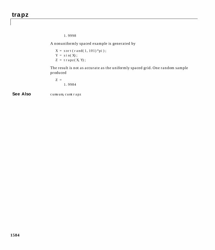
trapz
1584
1.9998
A nonuniformly spaced example is generated by
X = sort(rand(1,101)∗pi);Y = sin(X);Z = trapz(X,Y);
The result is not as accurate as the uniformly spaced grid. One random sampleproduced
Z =1.9984
See Also cumsum, cumtrapz
treelayout
1585
1treelayoutPurpose Lay out tree or forest
Syntax [x,y] = treelayout(parent,post)[x,y,h,s] = treelayout(parent,post)
Description [x,y] = treelayout(parent,post) lays out a tree or a forest. parent is thevector of parent pointers, with 0 for a root. post is an optional postorderpermutation on the tree nodes. If you omit post, treelayout computes it. x andy are vectors of coordinates in the unit square at which to lay out the nodes ofthe tree to make a nice picture.
[x,y,h,s] = treelayout(parent,post) also returns the height of the tree hand the number of vertices s in the top-level separator.
See Also etree, treeplot, etreeplot, symbfact
treeplot
1586
1treeplotPurpose Plot picture of tree
Syntax treeplot(p)treeplot(p,nodeSpec,edgeSpec)
Description treeplot(p) plots a picture of a tree given a vector of parent pointers, withp(i) = 0 for a root.
treeplot(p,nodeSpec,edgeSpec) allows optional parameters nodeSpec andedgeSpec to set the node or edge color, marker, and linestyle. Use '' to omitone or both.
See Also etree, etreeplot, treelayout
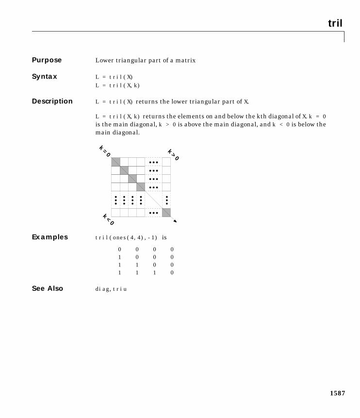
tril
1587
1trilPurpose Lower triangular part of a matrix
Syntax L = tril(X)L = tril(X,k)
Description L = tril(X) returns the lower triangular part of X.
L = tril(X,k) returns the elements on and below the kth diagonal of X. k = 0is the main diagonal, k > 0 is above the main diagonal, and k < 0 is below themain diagonal.
Examples tril(ones(4,4),-1) is
0 0 0 01 0 0 01 1 0 01 1 1 0
See Also diag, triu
k > 0
k < 0
k = 0
trimesh
1588
1trimeshPurpose Triangular mesh plot
Syntax trimesh(Tri,X,Y,Z)trimesh(Tri,X,Y,Z,C)trimesh(...'PropertyName',PropertyValue...)h = trimesh(...)
Description trimesh(Tri,X,Y,Z) displays triangles defined in the m-by-3 face matrix Trias a mesh. Each row of Tri defines a single triangular face by indexing into thevectors or matrices that contain the X, Y, and Z vertices.
trimesh(Tri,X,Y,Z,C) specifies color defined by C in the same manner as thesurf function. MATLAB performs a linear transformation on this data toobtain colors from the current colormap.
trimesh(...'PropertyName',PropertyValue...) specifies additional patchproperty names and values for the patch graphics object created by thefunction.
h = trimesh(...) returns a handle to a patch graphics object.
Example Create vertex vectors and a face matrix, then create a triangular mesh plot.
x = rand(1,50);y = rand(1,50);z = peaks(6*x–3,6*x–3);tri = delaunay(x,y);trimesh(tri,x,y,z)
See Also patch, trisurf, delaunay
trisurf
1589
1trisurfPurpose Triangular surface plot
Syntax trisurf(Tri,X,Y,Z)trisurf(Tri,X,Y,Z,C)trisurf(...'PropertyName',PropertyValue...)h = trisurf(...)
Description trisurf(Tri,X,Y,Z) displays triangles defined in the m-by-3 face matrix Trias a surface. Each row of Tri defines a single triangular face by indexing intothe vectors or matrices that contain the X, Y, and Z vertices.
trisurf(Tri,X,Y,Z,C) specifies color defined by C in the same manner as thesurf function. MATLAB performs a linear transformation on this data toobtain colors from the current colormap.
trisurf(...'PropertyName',PropertyValue...) specifies additional patchproperty names and values for the patch graphics object created by thefunction.
h = trisurf(...) returns a patch handle.
Example Create vertex vectors and a face matrix, then create a triangular surface plot.
x = rand(1,50);y = rand(1,50);z = peaks(6*x–3,6*x–3);tri = delaunay(x,y);trisurf(tri,x,y,z)
See Also patch, surf, trimesh, delaunay
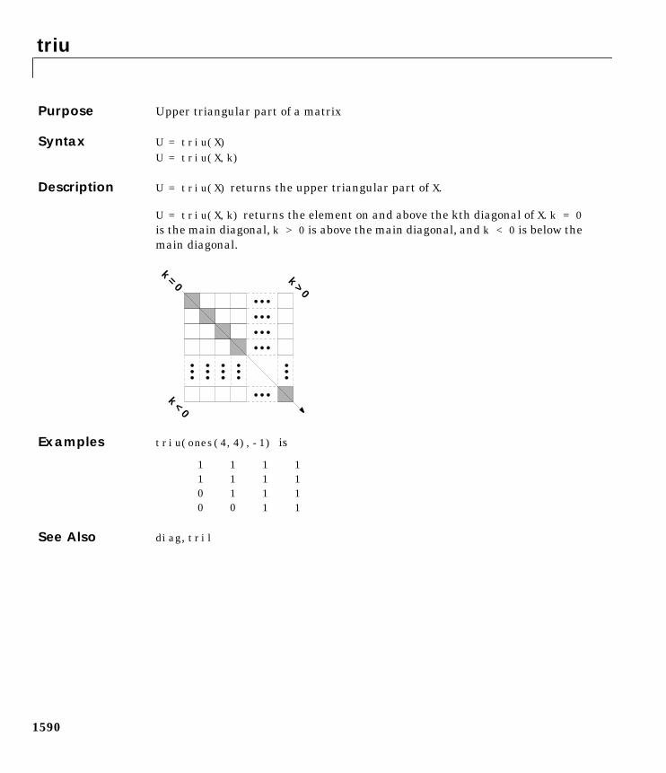
triu
1590
1triuPurpose Upper triangular part of a matrix
Syntax U = triu(X)U = triu(X,k)
Description U = triu(X) returns the upper triangular part of X.
U = triu(X,k) returns the element on and above the kth diagonal of X. k = 0is the main diagonal, k > 0 is above the main diagonal, and k < 0 is below themain diagonal.
Examples triu(ones(4,4),-1) is
1 1 1 11 1 1 10 1 1 10 0 1 1
See Also diag, tril
k > 0
k < 0
k = 0
try
1591
1tryPurpose Begin try block
Description The general form of a try statement is:
try,statement,...,statement,
catch,statement,...,statement,
end
Normally, only the statements between the try and catch are executed.However, if an error occurs while executing any of the statements, the error iscaptured into lasterr, and the statements between the catch and end areexecuted. If an error occurs within the catch statements, execution stopsunless caught by another try...catch block. The error string produced by afailed try block can be obtained with lasterr.
See Also catch, end, eval, evalin
tsearch
1592
1tsearchPurpose Search for enclosing Delaunay triangle
Syntax T = tsearch(x,y,TRI,xi,yi)
Description T = tsearch(x,y,TRI,xi,yi) returns an index into the rows of TRI for eachpoint in xi,yi. The tsearch command returns NaN for all points outside theconvex hull. Requires a triangulation TRI of the points x,y obtained fromdelaunay.
Note tsearch is based on qhull [1]. For information about qhull, seehttp://www.geom.umn.edu/software/qhull/. For copyright information, seehttp://www.geom.umn.edu/software/download/COPYING.html.
See Also delaunay, delaunayn, dsearch, tsearchn
References [1] National Science and Technology Research Center for Computation andVisualization of Geometric Structures (The Geometry Center), University ofMinnesota. 1993.
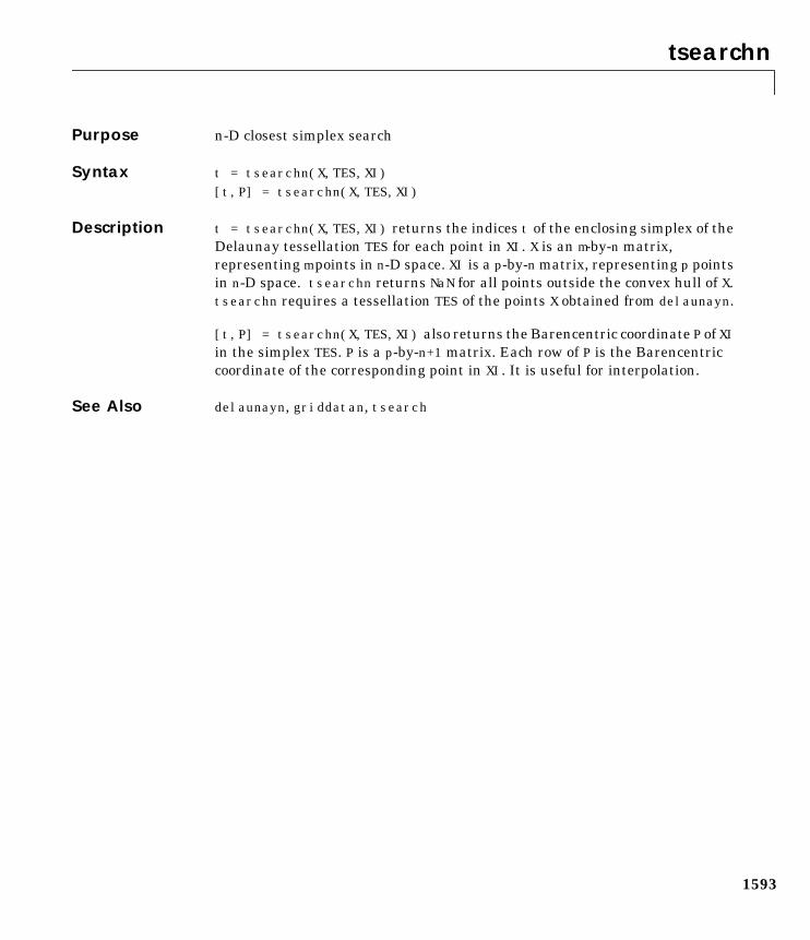
tsearchn
1593
1tsearchnPurpose n-D closest simplex search
Syntax t = tsearchn(X,TES,XI)[t,P] = tsearchn(X,TES,XI)
Description t = tsearchn(X,TES,XI) returns the indices t of the enclosing simplex of theDelaunay tessellation TES for each point in XI. X is an m-by-n matrix,representing m points in n-D space. XI is a p-by-n matrix, representing p pointsin n-D space. tsearchn returns NaN for all points outside the convex hull of X.tsearchn requires a tessellation TES of the points X obtained from delaunayn.
[t,P] = tsearchn(X,TES,XI) also returns the Barencentric coordinate P of XIin the simplex TES. P is a p-by-n+1 matrix. Each row of P is the Barencentriccoordinate of the corresponding point in XI. It is useful for interpolation.
See Also delaunayn, griddatan, tsearch
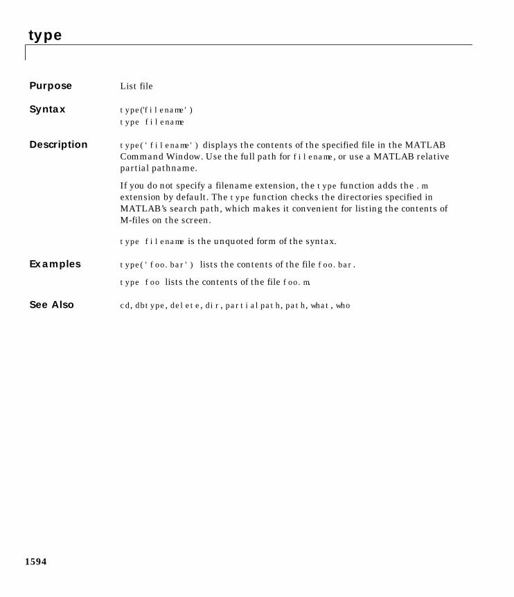
type
1594
1typePurpose List file
Syntax type('filename')type filename
Description type('filename') displays the contents of the specified file in the MATLABCommand Window. Use the full path for filename, or use a MATLAB relativepartial pathname.
If you do not specify a filename extension, the type function adds the .mextension by default. The type function checks the directories specified inMATLAB’s search path, which makes it convenient for listing the contents ofM-files on the screen.
type filename is the unquoted form of the syntax.
Examples type('foo.bar') lists the contents of the file foo.bar.
type foo lists the contents of the file foo.m.
See Also cd, dbtype, delete, dir, partialpath, path, what, who
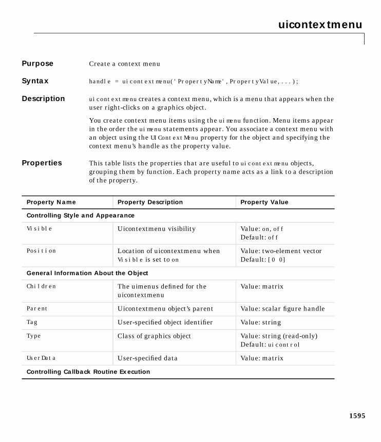
uicontextmenu
1595
1uicontextmenuPurpose Create a context menu
Syntax handle = uicontextmenu('PropertyName',PropertyValue,...);
Description uicontextmenu creates a context menu, which is a menu that appears when theuser right-clicks on a graphics object.
You create context menu items using the uimenu function. Menu items appearin the order the uimenu statements appear. You associate a context menu withan object using the UIContextMenu property for the object and specifying thecontext menu’s handle as the property value.
Properties This table lists the properties that are useful to uicontextmenu objects,grouping them by function. Each property name acts as a link to a descriptionof the property.
Property Name Property Description Property Value
Controlling Style and Appearance
Visible Uicontextmenu visibility Value: on, offDefault: off
Position Location of uicontextmenu whenVisible is set to on
Value: two-element vectorDefault: [0 0]
General Information About the Object
Children The uimenus defined for theuicontextmenu
Value: matrix
Parent Uicontextmenu object’s parent Value: scalar figure handle
Tag User-specified object identifier Value: string
Type Class of graphics object Value: string (read-only)Default: uicontrol
UserData User-specified data Value: matrix
Controlling Callback Routine Execution
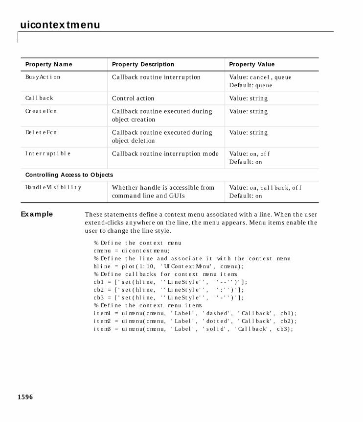
uicontextmenu
1596
Example These statements define a context menu associated with a line. When the userextend-clicks anywhere on the line, the menu appears. Menu items enable theuser to change the line style.
% Define the context menucmenu = uicontextmenu;% Define the line and associate it with the context menuhline = plot(1:10, 'UIContextMenu', cmenu);% Define callbacks for context menu itemscb1 = ['set(hline, ''LineStyle'', ''--'')'];cb2 = ['set(hline, ''LineStyle'', '':'')'];cb3 = ['set(hline, ''LineStyle'', ''-'')'];% Define the context menu itemsitem1 = uimenu(cmenu, 'Label', 'dashed', 'Callback', cb1);item2 = uimenu(cmenu, 'Label', 'dotted', 'Callback', cb2);item3 = uimenu(cmenu, 'Label', 'solid', 'Callback', cb3);
BusyAction Callback routine interruption Value: cancel, queueDefault: queue
Callback Control action Value: string
CreateFcn Callback routine executed duringobject creation
Value: string
DeleteFcn Callback routine executed duringobject deletion
Value: string
Interruptible Callback routine interruption mode Value: on, offDefault: on
Controlling Access to Objects
HandleVisibility Whether handle is accessible fromcommand line and GUIs
Value: on, callback, offDefault: on
Property Name Property Description Property Value
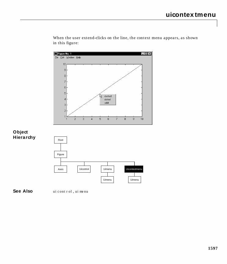
uicontextmenu
1597
When the user extend-clicks on the line, the context menu appears, as shownin this figure:
ObjectHierarchy
See Also uicontrol, uimenu
Root
UimenuAxes Uicontrol
Figure
Uicontextmenu
Uimenu Uimenu
uicontextmenu Properties
1598
1uicontextmenu PropertiesModifyingProperties
You can set and query graphics object properties in two ways:
• The Property Editor is an interactive tool that enables you to see and changeobject property values.
• The set and get commands enable you to set and query the values ofproperties
To change the default value of properties see Settingcreating_plots DefaultProperty Values.
UicontextmenuPropertyDescriptions
BusyAction cancel | queue
Callback routine interruption. The BusyAction property enables you to controlhow MATLAB handles events that potentially interrupt executing callbackroutines. If a callback routine is executing, subsequently invoked callbackroutines always attempt to interrupt it. If the Interruptible property of theobject whose callback is executing is set to on (the default), then interruptionoccurs at the next point where the event queue is processed. If theInterruptible property is off, the BusyAction property of the object whosecallback is executing determines how MATLAB handles the event. The choicesare:
• cancel – discard the event that attempted to execute a second callbackroutine.
• queue – queue the event that attempted to execute a second callback routineuntil the current callback finishes.
ButtonDownFcn string
This property has no effect on uicontextmenu objects.
Callback string
Control action. A routine that executes whenever you right-click on an objectfor which a context menu is defined. The routine executes immediately beforethe context menu is posted. Define this routine as a string that is a validMATLAB expression or the name of an M-file. The expression executes in theMATLAB workspace.
Children matrix
The uimenus defined for the uicontextmenu.
uicontextmenu Properties
1599
Clipping on | off
This property has no effect on uicontextmenu objects.
CreateFcn string
Callback routine executed during object creation. This property defines acallback routine that executes when MATLAB creates a uicontextmenu object.You must define this property as a default value for uicontextmenus. Forexample, this statement:
set(0,'DefaultUicontextmenuCreateFcn',...'set(gcf,''IntegerHandle'',''off'')')
defines a default value on the root level that sets the figure IntegerHandleproperty to off whenever you create a uicontextmenu object. MATLABexecutes this routine after setting all property values for the uicontextmenu.Setting this property on an existing uicontextmenu object has no effect.
The handle of the object whose CreateFcn is being executed is accessible onlythrough the root CallbackObject property, which can be queried using gcbo.
DeleteFcn string
Delete uicontextmenu callback routine. A callback routine that executes whenyou delete the uicontextmenu object (e.g., when you issue a delete commandor clear the figure containing the uicontextmenu). MATLAB executes theroutine before destroying the object’s properties so these values are availableto the callback routine.
The handle of the object whose DeleteFcn is being executed is accessible onlythrough the root CallbackObject property, which you can query using gcbo.
HandleVisibility on | callback | off
Control access to object’s handle by command-line users and GUIs. Thisproperty determines when an object’s handle is visible in its parent’s list ofchildren. HandleVisibility is useful for preventing command-line users fromaccidentally drawing into or deleting a figure that contains only user interfacedevices (such as a dialog box).
Handles are always visible when HandleVisibility is on.
Setting HandleVisibility to callback causes handles to be visible fromwithin callback routines or functions invoked by callback routines, but not from
uicontextmenu Properties
1600
within functions invoked from the command line. This provides a means toprotect GUIs from command-line users, while allowing callback routines tohave complete access to object handles.
Setting HandleVisibility to off makes handles invisible at all times. Thismay be necessary when a callback routine invokes a function that mightpotentially damage the GUI (such as evaluating a user-typed string), and sotemporarily hides its own handles during the execution of that function.
When a handle is not visible in its parent’s list of children, it cannot be returnedby functions that obtain handles by searching the object hierarchy or queryinghandle properties. This includes get, findobj, gca, gcf, gco, newplot, cla, clf,and close.
When a handle’s visibility is restricted using callback or off, the object’shandle does not appear in its parent’s Children property, figures do not appearin the root’s CurrentFigure property, objects do not appear in the root’sCallbackObject property or in the figure’s CurrentObject property, and axesdo not appear in their parent’s CurrentAxes property.
You can set the root ShowHiddenHandles property to on to make all handlesvisible, regardless of their HandleVisibility settings (this does not affect thevalues of the HandleVisibility properties).
Handles that are hidden are still valid. If you know an object’s handle, you canset and get its properties, and pass it to any function that operates on handles.
HitTest on | off
This property has no effect on uicontextmenu objects.
Interruptible on | off
Callback routine interruption mode. The Interruptible property controlswhether a uicontextmenu callback routine can be interrupted by subsequentlyinvoked callback routines. By default (on), execution of a callback routine canbe interrupted.
Only callback routines defined for the ButtonDownFcn and Callback propertiesare affected by the Interruptible property. MATLAB checks for events thatcan interrupt a callback routine only when it encounters a drawnow, figure,getframe, pause, or waitfor command in the routine.
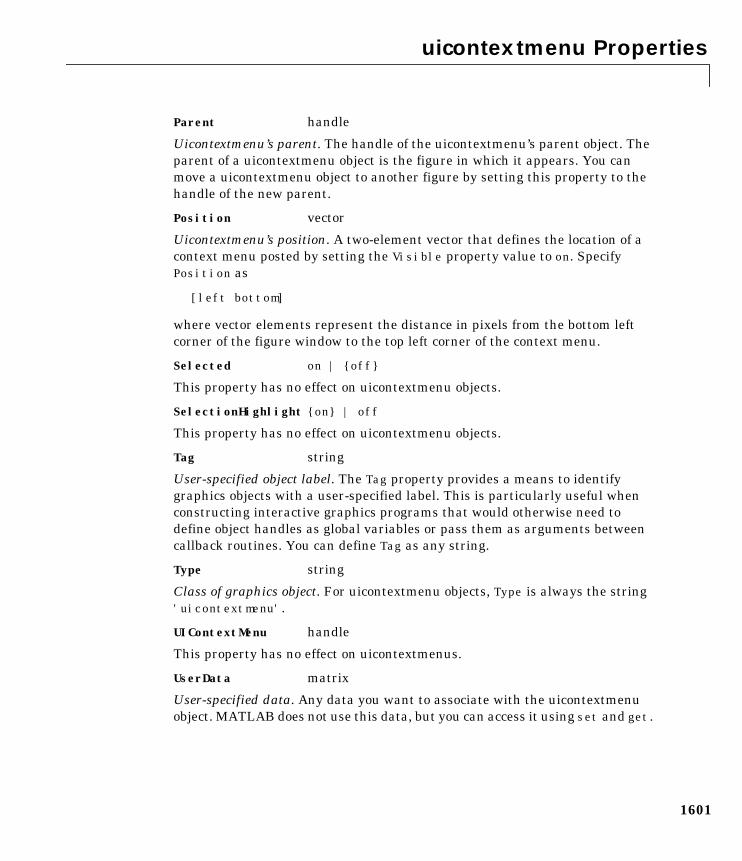
uicontextmenu Properties
1601
Parent handle
Uicontextmenu’s parent. The handle of the uicontextmenu’s parent object. Theparent of a uicontextmenu object is the figure in which it appears. You canmove a uicontextmenu object to another figure by setting this property to thehandle of the new parent.
Position vector
Uicontextmenu’s position. A two-element vector that defines the location of acontext menu posted by setting the Visible property value to on. SpecifyPosition as
[left bottom]
where vector elements represent the distance in pixels from the bottom leftcorner of the figure window to the top left corner of the context menu.
Selected on | off
This property has no effect on uicontextmenu objects.
SelectionHighlight on | off
This property has no effect on uicontextmenu objects.
Tag string
User-specified object label. The Tag property provides a means to identifygraphics objects with a user-specified label. This is particularly useful whenconstructing interactive graphics programs that would otherwise need todefine object handles as global variables or pass them as arguments betweencallback routines. You can define Tag as any string.
Type string
Class of graphics object. For uicontextmenu objects, Type is always the string'uicontextmenu'.
UIContextMenu handle
This property has no effect on uicontextmenus.
UserData matrix
User-specified data. Any data you want to associate with the uicontextmenuobject. MATLAB does not use this data, but you can access it using set and get.
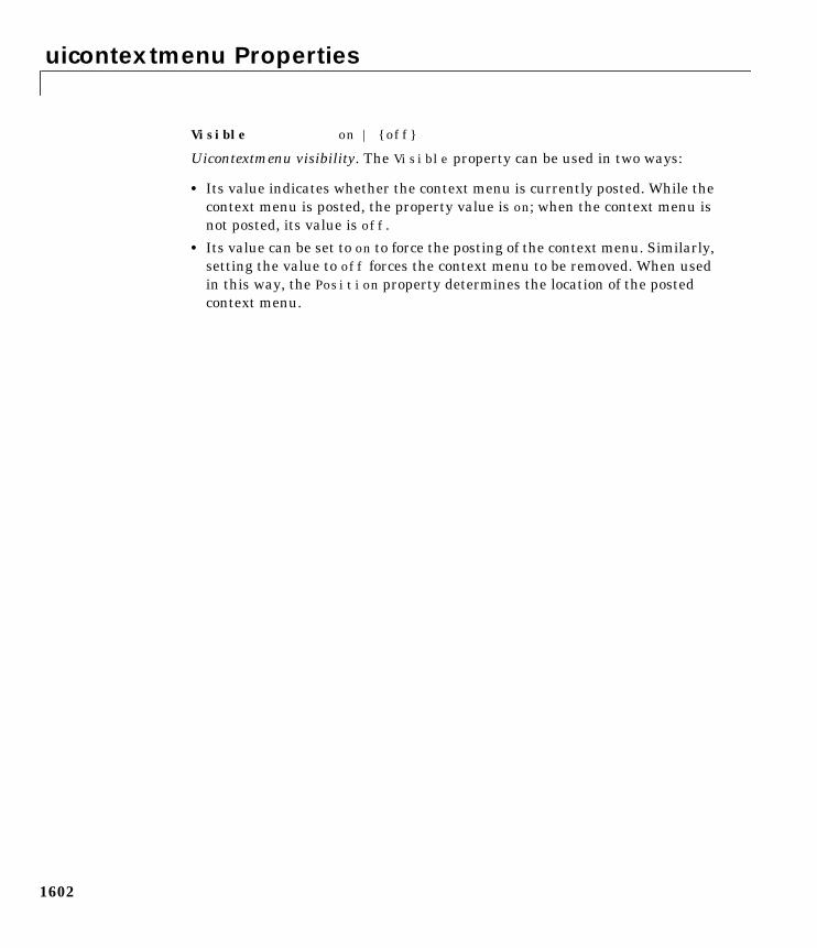
uicontextmenu Properties
1602
Visible on | off
Uicontextmenu visibility. The Visible property can be used in two ways:
• Its value indicates whether the context menu is currently posted. While thecontext menu is posted, the property value is on; when the context menu isnot posted, its value is off.
• Its value can be set to on to force the posting of the context menu. Similarly,setting the value to off forces the context menu to be removed. When usedin this way, the Position property determines the location of the postedcontext menu.
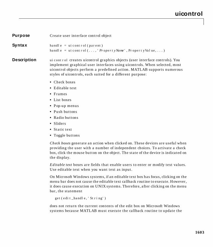
uicontrol
1603
1uicontrolPurpose Create user interface control object
Syntax handle = uicontrol(parent)handle = uicontrol(...,'PropertyName',PropertyValue,...)
Description uicontrol creates uicontrol graphics objects (user interface controls). Youimplement graphical user interfaces using uicontrols. When selected, mostuicontrol objects perform a predefined action. MATLAB supports numerousstyles of uicontrols, each suited for a different purpose:
• Check boxes
• Editable text
• Frames
• List boxes
• Pop-up menus
• Push buttons
• Radio buttons
• Sliders
• Static text
• Toggle buttons
Check boxes generate an action when clicked on. These devices are useful whenproviding the user with a number of independent choices. To activate a checkbox, click the mouse button on the object. The state of the device is indicated onthe display.
Editable text boxes are fields that enable users to enter or modify text values.Use editable text when you want text as input.
On Microsoft Windows systems, if an editable text box has focus, clicking on themenu bar does not cause the editable text callback routine to execute. However,it does cause execution on UNIX systems. Therefore, after clicking on the menubar, the statement
get(edit_handle,'String')
does not return the current contents of the edit box on Microsoft Windowssystems because MATLAB must execute the callback routine to update the
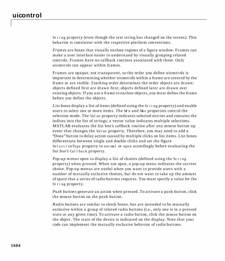
uicontrol
1604
String property (even though the text string has changed on the screen). Thisbehavior is consistent with the respective platform conventions.
Frames are boxes that visually enclose regions of a figure window. Frames canmake a user interface easier to understand by visually grouping relatedcontrols. Frames have no callback routines associated with them. Onlyuicontrols can appear within frames.
Frames are opaque, not transparent, so the order you define uicontrols isimportant in determining whether uicontrols within a frame are covered by theframe or are visible. Stacking order determines the order objects are drawn:objects defined first are drawn first; objects defined later are drawn overexisting objects. If you use a frame to enclose objects, you must define the framebefore you define the objects.
List boxes display a list of items (defined using the String property) and enableusers to select one or more items. The Min and Max properties control theselection mode. The Value property indicates selected entries and contains theindices into the list of strings; a vector value indicates multiple selections.MATLAB evaluates the list box’s callback routine after any mouse button upevent that changes the Value property. Therefore, you may need to add a“Done” button to delay action caused by multiple clicks on list items. List boxesdifferentiate between single and double clicks and set the figureSelectionType property to normal or open accordingly before evaluating thelist box’s Callback property.
Pop-up menus open to display a list of choices (defined using the Stringproperty) when pressed. When not open, a pop-up menu indicates the currentchoice. Pop-up menus are useful when you want to provide users with anumber of mutually exclusive choices, but do not want to take up the amountof space that a series of radio buttons requires. You must specify a value for theString property.
Push buttons generate an action when pressed. To activate a push button, clickthe mouse button on the push button.
Radio buttons are similar to check boxes, but are intended to be mutuallyexclusive within a group of related radio buttons (i.e., only one is in a pressedstate at any given time). To activate a radio button, click the mouse button onthe object. The state of the device is indicated on the display. Note that yourcode can implement the mutually exclusive behavior of radio buttons.
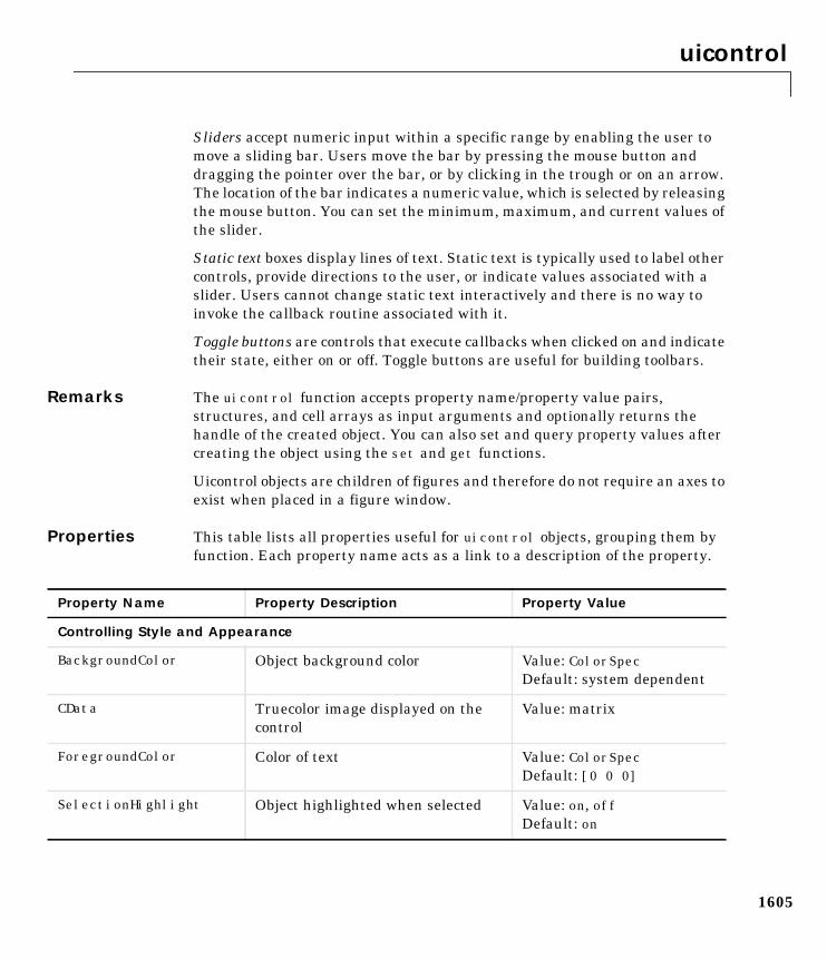
uicontrol
1605
Sliders accept numeric input within a specific range by enabling the user tomove a sliding bar. Users move the bar by pressing the mouse button anddragging the pointer over the bar, or by clicking in the trough or on an arrow.The location of the bar indicates a numeric value, which is selected by releasingthe mouse button. You can set the minimum, maximum, and current values ofthe slider.
Static text boxes display lines of text. Static text is typically used to label othercontrols, provide directions to the user, or indicate values associated with aslider. Users cannot change static text interactively and there is no way toinvoke the callback routine associated with it.
Toggle buttons are controls that execute callbacks when clicked on and indicatetheir state, either on or off. Toggle buttons are useful for building toolbars.
Remarks The uicontrol function accepts property name/property value pairs,structures, and cell arrays as input arguments and optionally returns thehandle of the created object. You can also set and query property values aftercreating the object using the set and get functions.
Uicontrol objects are children of figures and therefore do not require an axes toexist when placed in a figure window.
Properties This table lists all properties useful for uicontrol objects, grouping them byfunction. Each property name acts as a link to a description of the property.
Property Name Property Description Property Value
Controlling Style and Appearance
BackgroundColor Object background color Value: ColorSpecDefault: system dependent
CData Truecolor image displayed on thecontrol
Value: matrix
ForegroundColor Color of text Value: ColorSpecDefault: [0 0 0]
SelectionHighlight Object highlighted when selected Value: on, offDefault: on
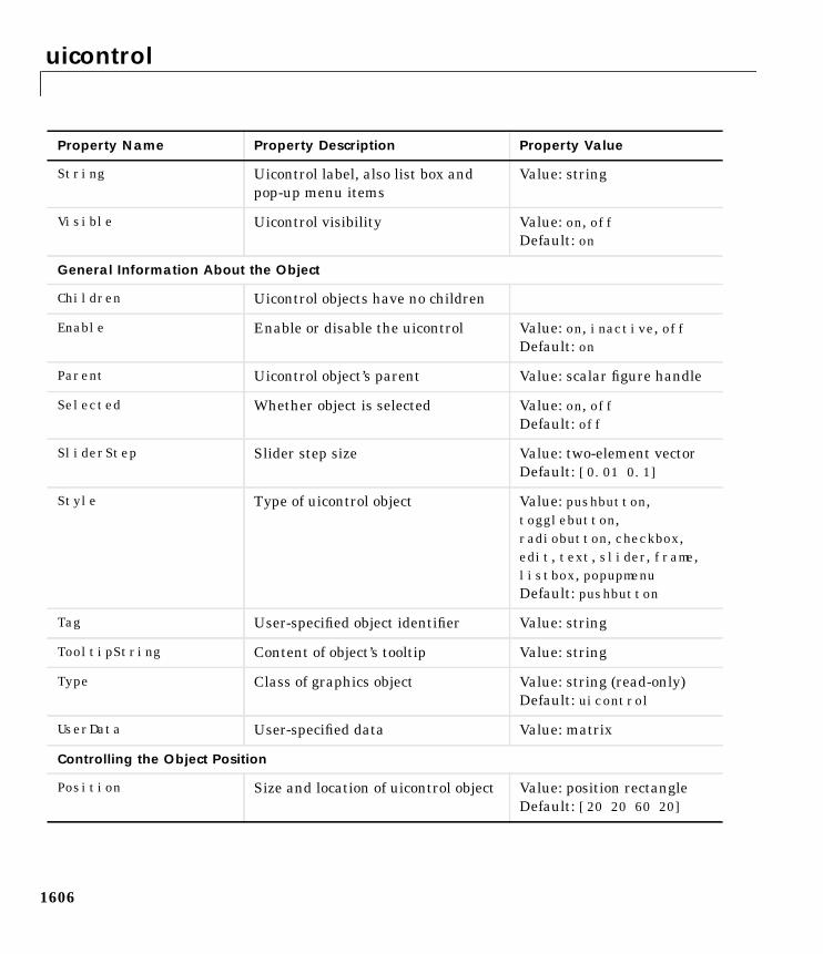
uicontrol
1606
String Uicontrol label, also list box andpop-up menu items
Value: string
Visible Uicontrol visibility Value: on, offDefault: on
General Information About the Object
Children Uicontrol objects have no children
Enable Enable or disable the uicontrol Value: on, inactive, offDefault: on
Parent Uicontrol object’s parent Value: scalar figure handle
Selected Whether object is selected Value: on, offDefault: off
SliderStep Slider step size Value: two-element vectorDefault: [0.01 0.1]
Style Type of uicontrol object Value: pushbutton,togglebutton,radiobutton, checkbox,edit, text, slider, frame,listbox, popupmenuDefault: pushbutton
Tag User-specified object identifier Value: string
TooltipString Content of object’s tooltip Value: string
Type Class of graphics object Value: string (read-only)Default: uicontrol
UserData User-specified data Value: matrix
Controlling the Object Position
Position Size and location of uicontrol object Value: position rectangleDefault: [20 20 60 20]
Property Name Property Description Property Value
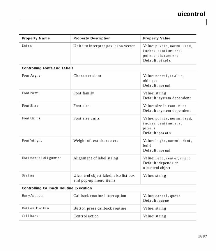
uicontrol
1607
Units Units to interpret position vector Value: pixels, normalized,inches, centimeters,points, charactersDefault: pixels
Controlling Fonts and Labels
FontAngle Character slant Value: normal, italic,obliqueDefault: normal
FontName Font family Value: stringDefault: system dependent
FontSize Font size Value: size in FontUnitsDefault: system dependent
FontUnits Font size units Value: points, normalized,inches, centimeters,pixelsDefault: points
FontWeight Weight of text characters Value: light, normal, demi,boldDefault: normal
HorizontalAlignment Alignment of label string Value: left, center, rightDefault: depends onuicontrol object
String Uicontrol object label, also list boxand pop-up menu items
Value: string
Controlling Callback Routine Execution
BusyAction Callback routine interruption Value: cancel, queueDefault: queue
ButtonDownFcn Button press callback routine Value: string
Callback Control action Value: string
Property Name Property Description Property Value
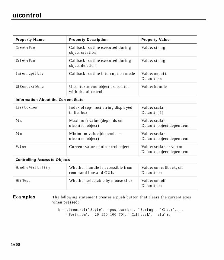
uicontrol
1608
Examples The following statement creates a push button that clears the current axeswhen pressed:
h = uicontrol('Style', 'pushbutton', 'String', 'Clear',...'Position', [20 150 100 70], 'Callback', 'cla');
CreateFcn Callback routine executed duringobject creation
Value: string
DeleteFcn Callback routine executed duringobject deletion
Value: string
Interruptible Callback routine interruption mode Value: on, offDefault: on
UIContextMenu Uicontextmenu object associatedwith the uicontrol
Value: handle
Information About the Current State
ListboxTop Index of top-most string displayedin list box
Value: scalarDefault: [1]
Max Maximum value (depends onuicontrol object)
Value: scalarDefault: object dependent
Min Minimum value (depends onuicontrol object)
Value: scalarDefault: object dependent
Value Current value of uicontrol object Value: scalar or vectorDefault: object dependent
Controlling Access to Objects
HandleVisibility Whether handle is accessible fromcommand line and GUIs
Value: on, callback, offDefault: on
HitTest Whether selectable by mouse click Value: on, offDefault: on
Property Name Property Description Property Value
uicontrol
1609
You can create a uicontrol object that changes figure colormaps by specifying apop-up menu and supplying an M-file name as the object’s Callback:
hpop = uicontrol('Style', 'popup',...'String', 'hsv|hot|cool|gray',...'Position', [20 320 100 50],...'Callback', 'setmap');
The above call to uicontrol defines four individual choices in the menu: hsv,hot, cool, and gray. You specify these choices with the String property,separating the choices with the “|” character.
The Callback, in this case setmap, is the name of an M-file that defines a morecomplicated set of instructions than a single MATLAB command. setmapcontains these statements:
val = get(hpop,'Value');if val == 1
colormap(hsv)elseif val == 2
colormap(hot)elseif val == 3
colormap(cool)elseif val == 4
colormap(gray)end
The Value property contains a number that indicates the selected choice. Thechoices are numbered sequentially from one to four. The setmap M-file can getand then test the contents of the Value property to determine what action totake.
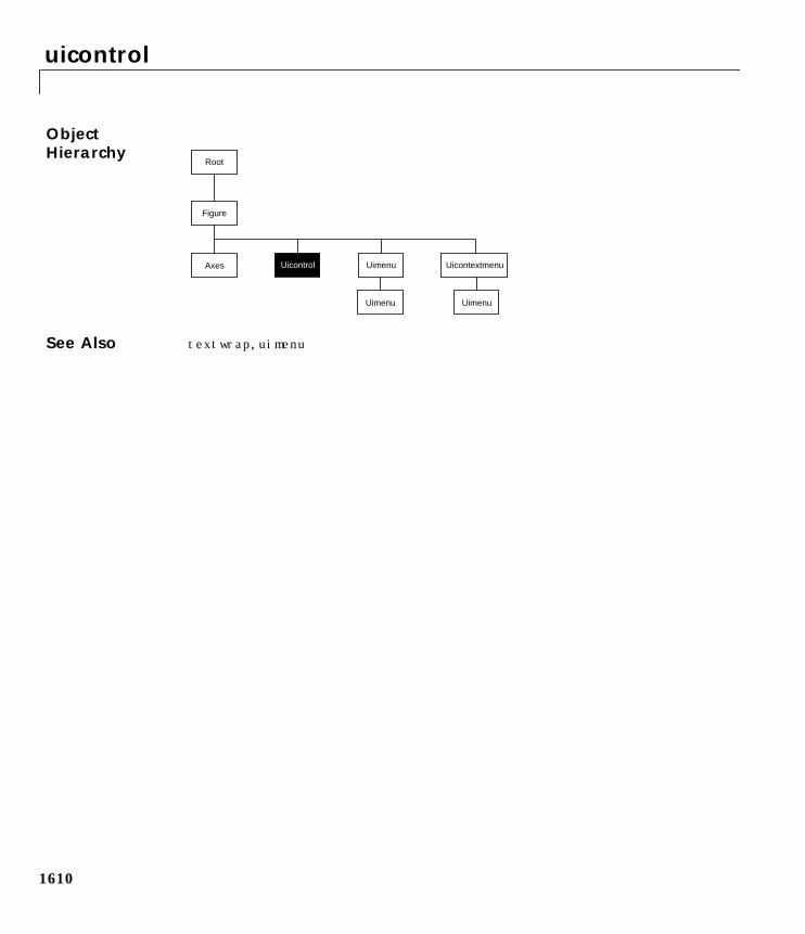
uicontrol
1610
ObjectHierarchy
See Also textwrap, uimenu
Root
UimenuAxes Uicontrol
Figure
Uicontextmenu
Uimenu Uimenu
Uicontrol Properties
1611
1Uicontrol PropertiesModifyingProperties
You can set and query graphics object properties in two ways:
• The Property Editor is an interactive tool that enables you to see and changeobject property values.
• The set and get commands enable you to set and query the values ofproperties
To change the default value of properties see Settingcreating_plots DefaultProperty Values.
UicontrolPropertyDescriptions
You can set default uicontrol properties on the root and figure levels:
set(0,'DefaultUicontrolProperty',PropertyValue...)set(gcf,'DefaultUicontrolProperty',PropertyValue...)
where Property is the name of the uicontrol property whose default value youwant to set and PropertyValue is the value you are specifying. Use set and getto access uicontrol properties.
Curly braces enclose the default value.
BackgroundColor ColorSpec
Object background color. The color used to fill the uicontrol rectangle. Specifya color using a three-element RGB vector or one of MATLAB’s predefinednames. The default color is determined by system settings. See ColorSpec formore information on specifying color.
BusyAction cancel | queue
Callback routine interruption. If a callback is executing and the user triggersan event (such as a mouse click) on an object for which a callback is defined,that callback attempts to interrupt the first callback. The first callback can beinterrupted only at a drawnow, figure, getframe, pause, or waitfor command;if the callback does not contain any of these commands, it cannot beinterrupted.
If the Interruptible property of the object whose callback is executing is off(the default value is on), the callback cannot be interrupted (except by certaincallbacks; see the note below). The BusyAction property of the object whosecallback is waiting to execute determines what happens to the callback:
Uicontrol Properties
1612
• If the value is queue, the callback is added to the event queue and executesafter the first callback finishes execution.
• If the value is cancel, the event is discarded and the callback is not executed.
Note If the interrupting callback is a DeleteFcn or CreateFcn callback or afigure’s CloseRequest or ResizeFcn callback, it interrupts an executingcallback regardless of the value of that object’s Interruptible property. Theinterrupting callback starts execution at the next drawnow, figure, getframe,pause, or waitfor statement.
ButtonDownFcn string
Button press callback routine. A callback routine that executes whenever youpress a mouse button while the pointer is in a five-pixel wide border around theuicontrol. When the uicontrol’s Enable property is set to inactive or off, theButtonDownFcn executes when you click the mouse in the five-pixel border oron the control itself. This is useful for implementing actions to interactivelymodify control object properties, such as size and position, when they areclicked on (using selectmoveresize, for example).
Define this routine as a string that is a valid MATLAB expression or the nameof an M-file. The expression executes in the MATLAB workspace.
The Callback property defines the callback routine that executes when youactivate the enabled uicontrol (e.g., click on a push button).
Callback string (GUIDE sets this property)
Control action. A routine that executes whenever you activate the uicontrolobject (e.g., when you click on a push button or move a slider). Define thisroutine as a string that is a valid MATLAB expression or the name of an M-file.The expression executes in the MATLAB workspace.
To execute the callback routine for an editable text control, type in the desiredtext, then either:
• Move the focus off the object (click the mouse someplace else in the GUI),
• For a single line editable text box, press Return, or
• For a multiline editable text box, press Ctl-Return .
Uicontrol Properties
1613
Callback routines defined for frames and static text do not execute because noaction is associated with these objects.
CData matrix
Truecolor image displayed on control. A three-dimensional matrix of RGBvalues that defines a truecolor image displayed on either a push button ortoggle button. Each value must be between 0.0 and 1.0.
Children matrix
The empty matrix; uicontrol objects have no children.
Clipping on | off
This property has no effect on uicontrols.
CreateFcn string
Callback routine executed during object creation. This property defines acallback routine that executes when MATLAB creates a uicontrol object. Youmust define this property as a default value for uicontrols. For example, thisstatement:
set(0,'DefaultUicontrolCreateFcn',...'set(gcf,''IntegerHandle'',''off'')')
defines a default value on the root level that sets the figure IntegerHandleproperty to off whenever you create a uicontrol object. MATLAB executes thisroutine after setting all property values for the uicontrol. Setting this propertyon an existing uicontrol object has no effect.
The handle of the object whose CreateFcn is being executed is accessible onlythrough the root CallbackObject property, which can be queried using gcbo.
DeleteFcn string
Delete uicontrol callback routine. A callback routine that executes when youdelete the uicontrol object (e.g., when you issue a delete command or clear thefigure containing the uicontrol). MATLAB executes the routine beforedestroying the object’s properties so these values are available to the callbackroutine.
The handle of the object whose DeleteFcn is being executed is accessible onlythrough the root CallbackObject property, which you can query using gcbo.
Uicontrol Properties
1614
Enable on | inactive | off
Enable or disable the uicontrol. This property controls how uicontrols respondto mouse button clicks, including which callback routines execute.
• on – The uicontrol is operational (the default).
• inactive – The uicontrol is not operational, but looks the same as whenEnable is on.
• off – The uicontrol is not operational and its label (set by the stringproperty) is grayed out.
When you left-click on a uicontrol whose Enable property is on, MATLABperforms these actions in this order:
1 Sets the figure’s SelectionType property.
2 Executes the control’s Callback routine.
3 Does not set the figure’s CurrentPoint property and does not execute eitherthe control’s ButtonDownFcn or the figure’s WindowButtonDownFcn callback.
When you left-click on a uicontrol whose Enable property is inactive or off,or when you right-click on a uicontrol whose Enable property has any value,MATLAB performs these actions in this order:
1 Sets the figure’s SelectionType property.
2 Sets the figure’s CurrentPoint property.
3 Executes the figure’s WindowButtonDownFcn callback.
4 On a right-click, if the uicontrol is associated with a context menu, posts thecontext menu.
5 Executes the control’s ButtonDownFcn callback.
6 Executes the selected context menu item’s Callback routine.
7 Does not execute the control’s Callback routine.
Setting this property to inactive or off enables you to implement objectdragging or resizing using the ButtonDownFcn callback routine.
Uicontrol Properties
1615
Extent position rectangle (read only)
Size of uicontrol character string. A four-element vector that defines the sizeand position of the character string used to label the uicontrol. It has the form:
[0,0,width,height]
The first two elements are always zero. width and height are the dimensionsof the rectangle. All measurements are in units specified by the Units property.
Since the Extent property is defined in the same units as the uicontrol itself,you can use this property to determine proper sizing for the uicontrol withregard to its label. Do this by
• Defining the String property and selecting the font using the relevantproperties.
• Getting the value of the Extent property.
• Defining the width and height of the Position property to be somewhatlarger than the width and height of the Extent.
For multiline strings, the Extent rectangle encompasses all the lines of text.For single line strings, the Extent is returned as a single line, even if the stringwraps when displayed on the control.
FontAngle normal | italic | oblique
Character slant. MATLAB uses this property to select a font from thoseavailable on your particular system. Setting this property to italic or obliqueselects a slanted version of the font, when it is available on your system.
FontName string
Font family. The name of the font in which to display the String. To displayand print properly, this must be a font that your system supports. The defaultfont is system dependent.
To use a fixed-width font that looks good in any locale (and displays properly inJapan, where multibyte character sets are used), set FontName to the stringFixedWidth (this string value is case sensitive):
set(uicontrol_handle, 'FontName', 'FixedWidth')
This parameter value eliminates the need to hard code the name of afixed-width font, which may not display text properly on systems that do not
Uicontrol Properties
1616
use ASCII character encoding (such as in Japan). A properly written MATLABapplication that needs to use a fixed-width font should set FontName toFixedWidth and rely on the root FixedWidthFontName property to be setcorrectly in the end user’s environment.
End users can adapt a MATLAB application to different locales or personalenvironments by setting the root FixedWidthFontName property to theappropriate value for that locale from startup.m. Setting the rootFixedWidthFontName property causes an immediate update of the display touse the new font.
FontSize size in FontUnits
Font size. A number specifying the size of the font in which to display theString, in units determined by the FontUnits property. The default point sizeis system dependent.
FontUnits points | normalized | inches |centimeters | pixels
Font size units. This property determines the units used by the FontSizeproperty. Normalized units interpret FontSize as a fraction of the height of theuicontrol. When you resize the uicontrol, MATLAB modifies the screenFontSize accordingly. pixels, inches, centimeters, and points are absoluteunits (1 point = 1/72 inch).
FontWeight light | normal | demi | bold
Weight of text characters. MATLAB uses this property to select a font fromthose available on your particular system. Setting this property to bold causesMATLAB to use a bold version of the font, when it is available on your system.
ForegroundColor ColorSpec
Color of text. This property determines the color of the text defined for theString property (the uicontrol label). Specify a color using a three-elementRGB vector or one of MATLAB ’s predefined names. The default text color isblack. See ColorSpec for more information on specifying color.
HandleVisibility on | callback | off
Control access to object’s handle by command-line users and GUIs. Thisproperty determines when an object’s handle is visible in its parent’s list ofchildren. HandleVisibility is useful for preventing command-line users from
Uicontrol Properties
1617
accidentally drawing into or deleting a figure that contains only user interfacedevices (such as a dialog box).
Handles are always visible when HandleVisibility is on.
Setting HandleVisibility to callback causes handles to be visible fromwithin callback routines or functions invoked by callback routines, but not fromwithin functions invoked from the command line. This provides a means toprotect GUIs from command-line users, while allowing callback routines tohave complete access to object handles.
Setting HandleVisibility to off makes handles invisible at all times. Thismay be necessary when a callback routine invokes a function that mightpotentially damage the GUI (such as evaluating a user-typed string), and sotemporarily hides its own handles during the execution of that function.
When a handle is not visible in its parent’s list of children, it cannot be returnedby functions that obtain handles by searching the object hierarchy or queryinghandle properties. This includes get, findobj, gca, gcf, gco, newplot, cla, clf,and close.
When a handle’s visibility is restricted using callback or off, the object’shandle does not appear in its parent’s Children property, figures do not appearin the root’s CurrentFigure property, objects do not appear in the root’sCallbackObject property or in the figure’s CurrentObject property, and axesdo not appear in their parent’s CurrentAxes property.
You can set the root ShowHiddenHandles property to on to make all handlesvisible, regardless of their HandleVisibility settings (this does not affect thevalues of the HandleVisibility properties).
Handles that are hidden are still valid. If you know an object’s handle, you canset and get its properties, and pass it to any function that operates on handles.
HitTest on | off
Selectable by mouse click. This property has no effect on uicontrol objects.
HorizontalAlignment left | center | right
Horizontal alignment of label string. This property determines the justificationof the text defined for the String property (the uicontrol label):
Uicontrol Properties
1618
• left — Text is left justified with respect to the uicontrol.
• center — Text is centered with respect to the uicontrol.
• right — Text is right justified with respect to the uicontrol.
On Microsoft Windows systems, this property affects only edit and textuicontrols.
Interruptible on | off
Callback routine interruption mode. If a callback is executing and the usertriggers an event (such as a mouse click) on an object for which a callback isdefined, that callback attempts to interrupt the first callback. MATLABprocesses the callbacks according to these factors:
• The Interruptible property of the object whose callback is executing
• Whether the executing callback contains drawnow, figure, getframe, pause,or waitfor statements
• The BusyAction property of the object whose callback is waiting to execute
If the Interruptible property of the object whose callback is executing is on(the default), the callback can be interrupted. The callback interrupts executionat the next drawnow, figure, getframe, pause, or waitfor statement, andprocesses the events in the event queue, which includes the waiting callback.
If the Interruptible property of the object whose callback is executing is off,the callback cannot be interrupted (except by certain callbacks; see the notebelow). The BusyAction property of the object whose callback is waiting toexecute determines what happens to the callback.
Note If the interrupting callback is a DeleteFcn or CreateFcn callback or afigure’s CloseRequest or ResizeFcn callback, it interrupts an executingcallback regardless of the value of that object’s Interruptible property. Theinterrupting callback starts execution at the next drawnow, figure, getframe,pause, or waitfor statement. A figure’s WindowButtonDownFcn callbackroutine, or an object’s ButtonDownFcn or Callback routine are processedaccording to the rules described above.
Uicontrol Properties
1619
ListboxTop scalar
Index of top-most string displayed in list box. This property applies only to thelistbox style of uicontrol. It specifies which string appears in the top-mostposition in a list box that is not large enough to display all list entries.ListboxTop is an index into the array of strings defined by the String propertyand must have a value between 1 and the number of strings. Noninteger valuesare fixed to the next lowest integer.
Max scalar
Maximum value. This property specifies the largest value allowed for the Valueproperty. Different styles of uicontrols interpret Max differently:
• Check boxes – Max is the setting of the Value property while the check box isselected.
• Editable text – If Max − Min > 1, then editable text boxes accept multilineinput. If Max − Min <= 1, then editable text boxes accept only single line input.
• List boxes – If Max − Min > 1, then list boxes allow multiple item selection. IfMax − Min <= 1, then list boxes do not allow multiple item selection.
• Radio buttons – Max is the setting of the Value property when the radiobutton is selected.
• Sliders – Max is the maximum slider value and must be greater than the Minproperty. The default is 1.
• Toggle buttons – Max is the value of the Value property when the togglebutton is selected. The default is 1.
• Frames, pop-up menus, push buttons, and static text do not use the Maxproperty.
Min scalar
Minimum value. This property specifies the smallest value allowed for theValue property. Different styles of uicontrols interpret Min differently:
• Check boxes – Min is the setting of the Value property while the check box isnot selected.
• Editable text – If Max − Min > 1, then editable text boxes accept multilineinput. If Max − Min <= 1, then editable text boxes accept only single line input.
• List boxes – If Max − Min > 1, then list boxes allow multiple item selection. IfMax − Min <= 1, then list boxes allow only single item selection.
Uicontrol Properties
1620
• Radio buttons – Min is the setting of the Value property when the radiobutton is not selected.
• Sliders – Min is the minimum slider value and must be less than Max. Thedefault is 0.
• Toggle buttons – Min is the value of the Value property when the togglebutton is not selected. The default is 0.
• Frames, pop-up menus, push buttons, and static text do not use the Minproperty.
Parent handle
Uicontrol’s parent. The handle of the uicontrol’s parent object. The parent of auicontrol object is the figure in which it appears. You can move a uicontrolobject to another figure by setting this property to the handle of the new parent.
Position position rectangle
Size and location of uicontrol. The rectangle defined by this property specifiesthe size and location of the control within the figure window. Specify Positionas
[left bottom width height]
left and bottom are the distance from the lower-left corner of the figurewindow to the lower-left corner of the uicontrol object. width and height arethe dimensions of the uicontrol rectangle. All measurements are in unitsspecified by the Units property.
On Microsoft Windows systems, the height of pop-up menus is automaticallydetermined by the size of the font. The value you specify for the height of thePosition property has no effect.
The width and height values determine the orientation of sliders. If width isgreater than height, then the slider is oriented horizontally, If height isgreater than width, then the slider is oriented vertically.
Selected on | off
Is object selected. When this property is on, MATLAB displays selection handlesif the SelectionHighlight property is also on. You can, for example, define theButtonDownFcn to set this property, allowing users to select the object with themouse.
Uicontrol Properties
1621
SelectionHighlight on | off
Object highlight when selected. When the Selected property is on, MATLABindicates the selected state by drawing four edge handles and four cornerhandles. When SelectionHighlight is off, MATLAB does not draw thehandles.
SliderStep [min_step max_step]
Slider step size. This property controls the amount the slider Value changeswhen you click the mouse on the arrow button (min_step) or on the slidertrough (max_step). Specify SliderStep as a two-element vector; each valuemust be in the range [0, 1]. The actual step size is a function of the specifiedSliderStep and the total slider range (Max − Min). The default, [0.01 0.10],provides a 1 percent change for clicks on the arrow button and a 10 percentchange for clicks in the trough.
For example, if you create the following slider,
uicontrol('Style','slider','Min',1,'Max',7,...'SliderStep',[0.1 0.6])
clicking on the arrow button moves the indicator by,
0.1*(7–1)ans =
0.6000
and clicking in the trough moves the indicator by,
0.6*(7–1)ans =
3.6000
Note that if the specified step size moves the slider to a value outside the range,the indicator moves only to the Max or Min value.
See also the Max, Min, and Value properties.
String string
Uicontrol label, list box items, pop-up menu choices. For check boxes, editabletext, push buttons, radio buttons, static text, and toggle buttons, the textdisplayed on the object. For list boxes and pop-up menus, the set of entries oritems displayed in the object.
Uicontrol Properties
1622
For uicontrol objects that display only one line of text, if the string value isspecified as a cell array of strings or padded string matrix, only the first stringof a cell array or of a padded string matrix is displayed; the rest are ignored.Vertical slash (‘|’) characters are not interpreted as line breaks and insteadshow up in the text displayed in the uicontrol.
For multiple line editable text or static text controls, line breaks occur betweeneach row of the string matrix, each cell of a cell array of strings, and after any\n characters embedded in the string. Vertical slash (‘|’) characters are notinterpreted as line breaks, and instead show up in the text displayed in theuicontrol.
For multiple items on a list box or pop-up menu, you can specify items as a cellarray of strings, a padded string matrix, or within a string vector separated byvertical slash (‘|’) characters.
For editable text, this property value is set to the string entered by the user.
Style pushbutton | togglebutton | radiobutton |checkbox | edit | text | slider | frame |listbox | popupmenu
Style of uicontrol object to create. The Style property specifies the kind ofuicontrol to create. See the Description section for information on each type.
Tag string (GUIDE sets this property)
User-specified object label. The Tag property provides a means to identifygraphics objects with a user-specified label. This is particularly useful whenconstructing interactive graphics programs that would otherwise need todefine object handles as global variables or pass them as arguments betweencallback routines. You can define Tag as any string.
TooltipString string
Content of tooltip for object. The TooltipString property specifies the text ofthe tooltip associated with the uicontrol. When the user moves the mousepointer over the control and leaves it there, the tooltip is displayed.
Type string (read only)
Class of graphics object. For uicontrol objects, Type is always the string'uicontrol'.
Uicontrol Properties
1623
UIContextMenu handle
Associate a context menu with uicontrol. Assign this property the handle of aUicontextmenu object. MATLAB displays the context menu whenever youright-click over the uicontrol. Use the uicontextmenu function to create thecontext menu.
Units pixels | normalized | inches |centimeters | points | characters(Guide default normalized)
Units of measurement. The units MATLAB uses to interpret the Extent andPosition properties. All units are measured from the lower-left corner of thefigure window. Normalized units map the lower-left corner of the figurewindow to (0,0) and the upper-right corner to (1.0,1.0). pixels, inches,centimeters, and points are absolute units (1 point = 1/72 inch). Characterunits are characters using the default system font; the width of one characteris the width of the letter x, the height of one character is the distance betweenthe baselines of two lines of text.
If you change the value of Units, it is good practice to return it to its defaultvalue after completing your computation so as not to affect other functions thatassume Units is set to the default value.
UserData matrix
User-specified data. Any data you want to associate with the uicontrol object.MATLAB does not use this data, but you can access it using set and get.
Value scalar or vector
Current value of uicontrol. The uicontrol style determines the possible valuesthis property can have:
• Check boxes set Value to Max when they are on (when selected) and Min whenoff (not selected).
• List boxes set Value to a vector of indices corresponding to the selected listentries, where 1 corresponds to the first item in the list.
• Pop-up menus set Value to the index of the item selected, where 1corresponds to the first item in the menu. The Examples section shows howto use the Value property to determine which item has been selected.
• Radio buttons set Value to Max when they are on (when selected) and Minwhen off (not selected).
Uicontrol Properties
1624
• Sliders set Value to the number indicated by the slider bar.
• Toggle buttons set Value to Max when they are down (selected) and Min whenup (not selected).
• Editable text, frames, push buttons, and static text do not set this property.
Set the Value property either interactively with the mouse or through a call tothe set function. The display reflects changes made to Value.
Visible on | off
Uicontrol visibility. By default, all uicontrols are visible. When set to off, theuicontrol is not visible, but still exists and you can query and set its properties.
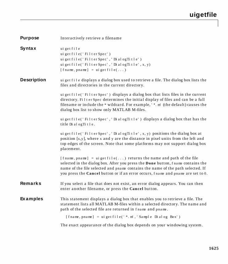
uigetfile
1625
1uigetfilePurpose Interactively retrieve a filename
Syntax uigetfileuigetfile('FilterSpec')uigetfile('FilterSpec','DialogTitle')uigetfile('FilterSpec','DialogTitle',x,y)[fname,pname] = uigetfile(...)
Description uigetfile displays a dialog box used to retrieve a file. The dialog box lists thefiles and directories in the current directory.
uigetfile('FilterSpec') displays a dialog box that lists files in the currentdirectory. FilterSpec determines the initial display of files and can be a fullfilename or include the * wildcard. For example, '∗.m' (the default) causes thedialog box list to show only MATLAB M-files.
uigetfile('FilterSpec','DialogTitle') displays a dialog box that has thetitle DialogTitle.
uigetfile('FilterSpec','DialogTitle',x,y) positions the dialog box atposition [x,y], where x and y are the distance in pixel units from the left andtop edges of the screen. Note that some platforms may not support dialog boxplacement.
[fname,pname] = uigetfile(...) returns the name and path of the fileselected in the dialog box. After you press the Done button, fname contains thename of the file selected and pname contains the name of the path selected. Ifyou press the Cancel button or if an error occurs, fname and pname are set to 0.
Remarks If you select a file that does not exist, an error dialog appears. You can thenenter another filename, or press the Cancel button.
Examples This statement displays a dialog box that enables you to retrieve a file. Thestatement lists all MATLAB M-files within a selected directory. The name andpath of the selected file are returned in fname and pname.
[fname,pname] = uigetfile('*.m','Sample Dialog Box')
The exact appearance of the dialog box depends on your windowing system.

uigetfile
1626
See Also uiputfile
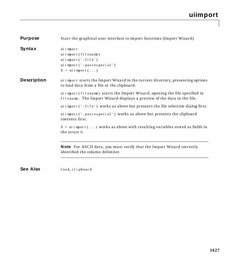
uiimport
1627
1uiimportPurpose Start the graphical user interface to import functions (Import Wizard)
Syntax uiimportuiimport(filename)uiimport('-file')uiimport('-pastespecial')S = uiimport(...)
Description uiimport starts the Import Wizard in the current directory, presenting optionsto load data from a file or the clipboard.
uiimport(filename) starts the Import Wizard, opening the file specified infilename. The Import Wizard displays a preview of the data in the file.
uiimport('-file') works as above but presents the file selection dialog first.
uiimport('-pastespecial') works as above but presents the clipboardcontents first.
S = uiimport(...) works as above with resulting variables stored as fields inthe struct S.
Note For ASCII data, you must verify that the Import Wizard correctlyidentified the column delimiter.
See Also load, clipboard
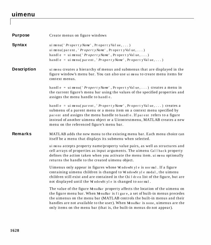
uimenu
1628
1uimenuPurpose Create menus on figure windows
Syntax uimenu('PropertyName',PropertyValue,...)uimenu(parent,'PropertyName',PropertyValue,...)handle = uimenu('PropertyName',PropertyValue,...)handle = uimenu(parent,'PropertyName',PropertyValue,...)
Description uimenu creates a hierarchy of menus and submenus that are displayed in thefigure window’s menu bar. You can also use uimenu to create menu items forcontext menus.
handle = uimenu('PropertyName',PropertyValue,...) creates a menu inthe current figure’s menu bar using the values of the specified properties andassigns the menu handle to handle.
handle = uimenu(parent,'PropertyName',PropertyValue,...) creates asubmenu of a parent menu or a menu item on a context menu specified byparent and assigns the menu handle to handle. If parent refers to a figureinstead of another uimenu object or a Uicontextmenu, MATLAB creates a newmenu on the referenced figure’s menu bar.
Remarks MATLAB adds the new menu to the existing menu bar. Each menu choice canitself be a menu that displays its submenu when selected.
uimenu accepts property name/property value pairs, as well as structures andcell arrays of properties as input arguments. The uimenu Callback propertydefines the action taken when you activate the menu item. uimenu optionallyreturns the handle to the created uimenu object.
Uimenus only appear in figures whose WindowStyle is normal. If a figurecontaining uimenu children is changed to WindowStyle modal, the uimenuchildren still exist and are contained in the Children list of the figure, but arenot displayed until the WindowStyle is changed to normal.
The value of the figure MenuBar property affects the location of the uimenu onthe figure menu bar. When MenuBar is figure, a set of built-in menus precedesthe uimenus on the menu bar (MATLAB controls the built-in menus and theirhandles are not available to the user). When MenuBar is none, uimenus are theonly items on the menu bar (that is, the built-in menus do not appear).
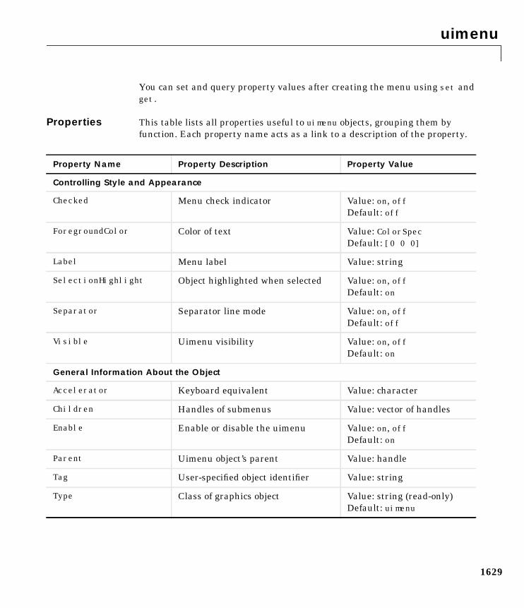
uimenu
1629
You can set and query property values after creating the menu using set andget.
Properties This table lists all properties useful to uimenu objects, grouping them byfunction. Each property name acts as a link to a description of the property.
Property Name Property Description Property Value
Controlling Style and Appearance
Checked Menu check indicator Value: on, offDefault: off
ForegroundColor Color of text Value: ColorSpecDefault: [0 0 0]
Label Menu label Value: string
SelectionHighlight Object highlighted when selected Value: on, offDefault: on
Separator Separator line mode Value: on, offDefault: off
Visible Uimenu visibility Value: on, offDefault: on
General Information About the Object
Accelerator Keyboard equivalent Value: character
Children Handles of submenus Value: vector of handles
Enable Enable or disable the uimenu Value: on, offDefault: on
Parent Uimenu object’s parent Value: handle
Tag User-specified object identifier Value: string
Type Class of graphics object Value: string (read-only)Default: uimenu
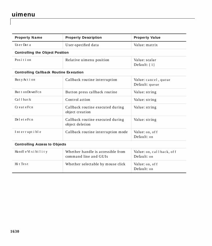
uimenu
1630
UserData User-specified data Value: matrix
Controlling the Object Position
Position Relative uimenu position Value: scalarDefault: [1]
Controlling Callback Routine Execution
BusyAction Callback routine interruption Value: cancel, queueDefault: queue
ButtonDownFcn Button press callback routine Value: string
Callback Control action Value: string
CreateFcn Callback routine executed duringobject creation
Value: string
DeleteFcn Callback routine executed duringobject deletion
Value: string
Interruptible Callback routine interruption mode Value: on, offDefault: on
Controlling Access to Objects
HandleVisibility Whether handle is accessible fromcommand line and GUIs
Value: on, callback, offDefault: on
HitTest Whether selectable by mouse click Value: on, offDefault: on
Property Name Property Description Property Value
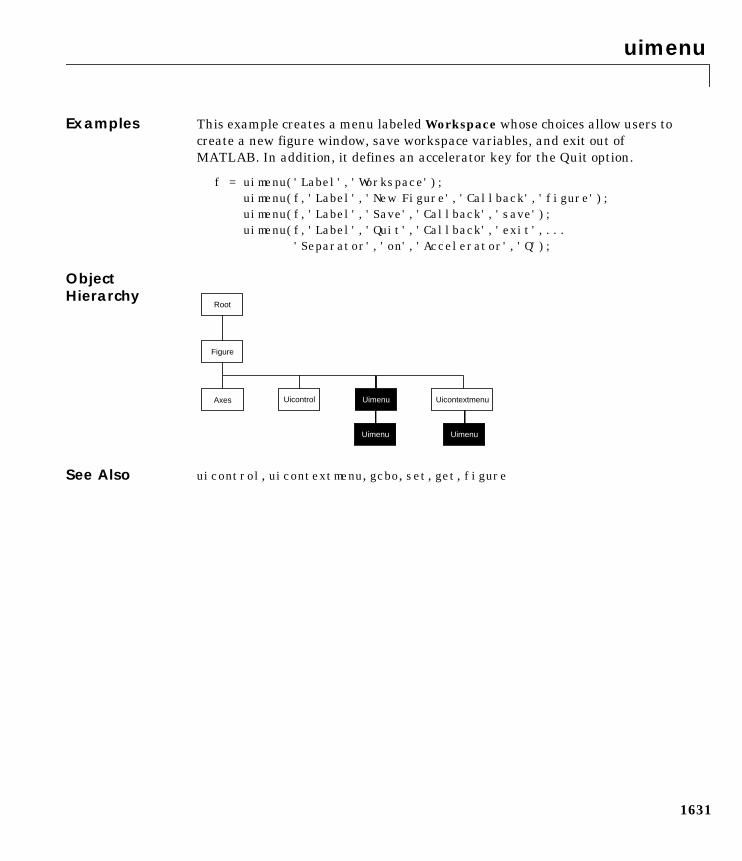
uimenu
1631
Examples This example creates a menu labeled Workspace whose choices allow users tocreate a new figure window, save workspace variables, and exit out ofMATLAB. In addition, it defines an accelerator key for the Quit option.
f = uimenu('Label','Workspace');uimenu(f,'Label','New Figure','Callback','figure');uimenu(f,'Label','Save','Callback','save');uimenu(f,'Label','Quit','Callback','exit',...
'Separator','on','Accelerator','Q');
ObjectHierarchy
See Also uicontrol, uicontextmenu, gcbo, set, get, figure
Root
UimenuAxes Uicontrol
Figure
Uicontextmenu
Uimenu Uimenu
Uimenu Properties
1632
1Uimenu PropertiesModifyingProperties
You can set and query graphics object properties in two ways:
• The Property Editor is an interactive tool that enables you to see and changeobject property values.
• The set and get commands enable you to set and query the values ofproperties
To change the default value of properties see Settingcreating_plots DefaultProperty Values.
UimenuProperties
This section lists property names along with the type of values each accepts.Curly braces enclose default values.
You can set default uimenu properties on the figure and root levels:
set(0,'DefaultUimenuPropertyName',PropertyValue...)set(gcf,'DefaultUimenuPropertyName',PropertyValue...)set(menu_handle,'DefaultUimenuProperty',PropertyValue...)
Where PropertyName is the name of the uimenu property and PropertyValueis the value you are specifying. Use set and get to access uimenu properties.
Accelerator character
Keyboard equivalent. A character specifying the keyboard equivalent for themenu item. This allows users to select a particular menu choice by pressing thespecified character in conjunction with another key, instead of selecting themenu item with the mouse. The key sequence is platform specific:
• For Microsoft Windows systems, the sequence is Ctrl-Accelerator. Thesekeys are reserved for default menu items: c, v, and x.
• For UNIX systems, the sequence is Ctrl-Accelerator. These keys arereserved for default menu items: o, p, s, and w.
You can define an accelerator only for menu items that do not have childrenmenus. Accelerators work only for menu items that directly execute a callbackroutine, not items that bring up other menus.
Note that the menu item does not have to be displayed (e.g., a submenu) for theaccelerator key to work. However, the window focus must be in the figure whenthe key sequence is entered.
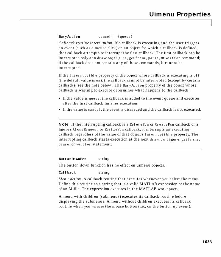
Uimenu Properties
1633
BusyAction cancel | queue
Callback routine interruption. If a callback is executing and the user triggersan event (such as a mouse click) on an object for which a callback is defined,that callback attempts to interrupt the first callback. The first callback can beinterrupted only at a drawnow, figure, getframe, pause, or waitfor command;if the callback does not contain any of these commands, it cannot beinterrupted.
If the Interruptible property of the object whose callback is executing is off(the default value is on), the callback cannot be interrupted (except by certaincallbacks; see the note below). The BusyAction property of the object whosecallback is waiting to execute determines what happens to the callback:
• If the value is queue, the callback is added to the event queue and executesafter the first callback finishes execution.
• If the value is cancel, the event is discarded and the callback is not executed.
Note If the interrupting callback is a DeleteFcn or CreateFcn callback or afigure’s CloseRequest or ResizeFcn callback, it interrupts an executingcallback regardless of the value of that object’s Interruptible property. Theinterrupting callback starts execution at the next drawnow, figure, getframe,pause, or waitfor statement.
ButtonDownFcn string
The button down function has no effect on uimenu objects.
Callback string
Menu action. A callback routine that executes whenever you select the menu.Define this routine as a string that is a valid MATLAB expression or the nameof an M-file. The expression executes in the MATLAB workspace.
A menu with children (submenus) executes its callback routine beforedisplaying the submenus. A menu without children executes its callbackroutine when you release the mouse button (i.e., on the button up event).
Uimenu Properties
1634
Checked on | off
Menu check indicator. Setting this property to on places a check mark next tothe corresponding menu item. Setting it to off removes the check mark. Youcan use this feature to create menus that indicate the state of a particularoption. Note that there is no formal mechanism for indicating that anunchecked menu item will become checked when selected. Also, this propertydoes not check top level menus or submenus, although you can change thevalue of the property for these menus.
Children vector of handles
Handles of submenus. A vector containing the handles of all children of theuimenu object. The children objects of uimenus are other uimenus, whichfunction as submenus. You can use this property to re-order the menus.
Clipping on | off
Clipping has no effect on uimenu objects.
CreateFcn string
Callback routine executed during object creation. This property defines acallback routine that executes when MATLAB creates a uimenu object. Youmust define this property as a default value for uimenus. For example, thestatement,
set(0,'DefaultUimenuCreateFcn','set(gcf,''IntegerHandle'',...''off''’))
defines a default value on the root level that sets the figure IntegerHandleproperty to off whenever you create a uimenu object. Setting this property onan existing uimenu object has no effect. MATLAB executes this routine aftersetting all property values for the uimenu.
The handle of the object whose CreateFcn is being executed is accessible onlythrough the root CallbackObject property, which can be queried using gcbo.
DeleteFcn string
Delete uimenu callback routine. A callback routine that executes when youdelete the uimenu object (e.g., when you issue a delete command or cause thefigure containing the uimenu to reset). MATLAB executes the routine beforedestroying the object’s properties so these values are available to the callbackroutine.
Uimenu Properties
1635
The handle of the object whose DeleteFcn is being executed is accessible onlythrough the root CallbackObject property, which is more simply queried usinggcbo.
Enable on | off
Enable or disable the uimenu. This property controls whether a menu item canbe selected. When not enabled (set to off), the menu Label appears dimmed,indicating the user cannot select it.
ForegroundColor ColorSpec X-Windows only
Color of menu label string. This property determines color of the text definedfor the Label property. Specify a color using a three-element RGB vector or oneof MATLAB’s predefined names. The default text color is black. See ColorSpecfor more information on specifying color.
HandleVisibility on | callback | off
Control access to object’s handle by command-line users and GUIs. Thisproperty determines when an object’s handle is visible in its parent’s list ofchildren. HandleVisibility is useful for preventing command-line users fromaccidentally drawing into or deleting a figure that contains only user interfacedevices (such as a dialog box).
Handles are always visible when HandleVisibility is on.
Setting HandleVisibility to callback causes handles to be visible fromwithin callback routines or functions invoked by callback routines, but not fromwithin functions invoked from the command line. This provide a means toprotect GUIs from command-line users, while allowing callback routines tohave complete access to object handles.
Setting HandleVisibility to off makes handles invisible at all times. Thismay be necessary when a callback routine invokes a function that mightpotentially damage the GUI (such as evaluating a user-typed string), and sotemporarily hides its own handles during the execution of that function.
When a handle is not visible in its parent’s list of children, it cannot be returnedby functions that obtain handles by searching the object hierarchy or queryinghandle properties. This includes get, findobj, gca, gcf, gco, newplot, cla, clf,and close.
Uimenu Properties
1636
When a handle’s visibility is restricted using callback or off, the object’shandle does not appear in its parent’s Children property, figures do not appearin the root’s CurrentFigure property, objects do not appear in the root’sCallbackObject property or in the figure’s CurrentObject property, and axesdo not appear in their parent’s CurrentAxes property.
You can set the root ShowHiddenHandles property to on to make all handlesvisible, regardless of their HandleVisibility settings (this does not affect thevalues of the HandleVisibility properties).
Handles that are hidden are still valid. If you know an object’s handle, you canset and get its properties, and pass it to any function that operates on handles.
Interruptible on | off
Callback routine interruption mode. If a callback is executing and the usertriggers an event (such as a mouse click) on an object for which a callback isdefined, that callback attempts to interrupt the first callback. MATLABprocesses the callbacks according to these factors:
• The Interruptible property of the object whose callback is executing
• Whether the executing callback contains drawnow, figure, getframe, pause,or waitfor statements
• The BusyAction property of the object whose callback is waiting to execute
If the Interruptible property of the object whose callback is executing is on(the default), the callback can be interrupted. The callback interruptsexecution at the next drawnow, figure, getframe, pause, or waitfor statement,and processes the events in the event queue, which includes the waitingcallback.
If the Interruptible property of the object whose callback is executing is off,the callback cannot be interrupted (except by certain callbacks; see the notebelow). The BusyAction property of the object whose callback is waiting toexecute determines what happens to the callback.
Note If the interrupting callback is a DeleteFcn or CreateFcn callback or afigure’s CloseRequest or ResizeFcn callback, it interrupts an executingcallback regardless of the value of that object’s Interruptible property. Theinterrupting callback starts execution at the next drawnow, figure, getframe,
Uimenu Properties
1637
pause, or waitfor statement. A figure’s WindowButtonDownFcn callbackroutine, or an object’s ButtonDownFcn or Callback routine are processedaccording to the rules described above.
Label string
Menu label. A string specifying the text label on the menu item. You can specifya mnemonic using the “&” character. Whatever character follows the “&” in thestring appears underlined and selects the menu item when you type thatcharacter while the menu is visible. The “&” character is not displayed. Todisplay the “&” character in a label, use two “&” characters in the string:
‘O&pen selection’ yields Open selection
‘Save && Go’ yields Save & Go
Parent handle
Uimenu’s parent. The handle of the uimenu’s parent object. The parent of auimenu object is the figure on whose menu bar it displays, or the uimenu ofwhich it is a submenu. You can move a uimenu object to another figure bysetting this property to the handle of the new parent.
Position scalar
Relative menu position. The value of Position indicates placement on themenu bar or within a menu. Top-level menus are placed from left to right onthe menu bar according to the value of their Position property, with 1representing the left-most position. The individual items within a given menuare placed from top to bottom according to the value of their Position property,with 1 representing the top-most position.
Selected on | off
This property is not used for uimenu objects.
SelectionHighlight on | off
This property is not used for uimenu objects.
Separator on | off
Separator line mode. Setting this property to on draws a dividing line above themenu item.
Uimenu Properties
1638
Tag string
User-specified object label. The Tag property provides a means to identifygraphics objects with a user-specified label. This is particularly useful whenconstructing interactive graphics programs that would otherwise need todefine object handles as global variables or pass them as arguments betweencallback routines. You can define Tag as any string.
Type string (read only)
Class of graphics object. For uimenu objects, Type is always the string'uimenu'.
UserData matrix
User-specified data. Any matrix you want to associate with the uimenu object.MATLAB does not use this data, but you can access it using the set and getcommands.
Visible on | off
Uimenu visibility. By default, all uimenus are visible. When set to off, theuimenu is not visible, but still exists and you can query and set its properties.
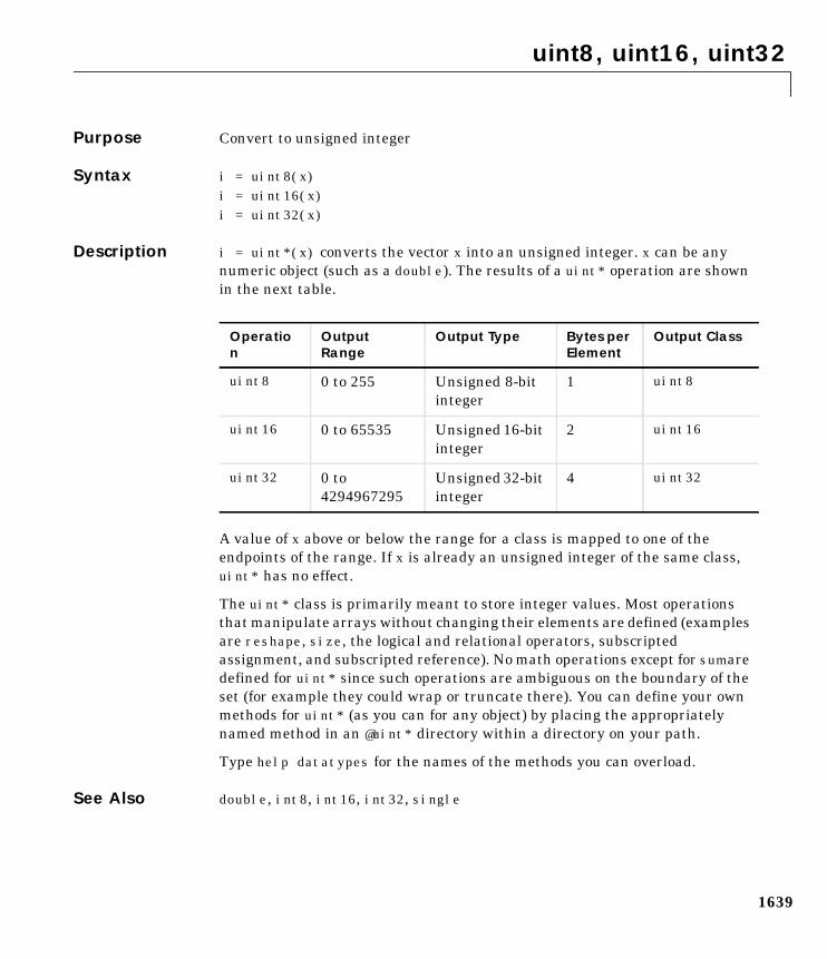
uint8, uint16, uint32
1639
1uint8, uint16, uint32Purpose Convert to unsigned integer
Syntax i = uint8(x)i = uint16(x)i = uint32(x)
Description i = uint*(x) converts the vector x into an unsigned integer. x can be anynumeric object (such as a double). The results of a uint* operation are shownin the next table.
A value of x above or below the range for a class is mapped to one of theendpoints of the range. If x is already an unsigned integer of the same class,uint* has no effect.
The uint* class is primarily meant to store integer values. Most operationsthat manipulate arrays without changing their elements are defined (examplesare reshape, size, the logical and relational operators, subscriptedassignment, and subscripted reference). No math operations except for sum aredefined for uint* since such operations are ambiguous on the boundary of theset (for example they could wrap or truncate there). You can define your ownmethods for uint* (as you can for any object) by placing the appropriatelynamed method in an @uint* directory within a directory on your path.
Type help datatypes for the names of the methods you can overload.
See Also double, int8, int16, int32, single
Operation
OutputRange
Output Type Bytes perElement
Output Class
uint8 0 to 255 Unsigned 8-bitinteger
1 uint8
uint16 0 to 65535 Unsigned 16-bitinteger
2 uint16
uint32 0 to4294967295
Unsigned 32-bitinteger
4 uint32
uiputfile
1640
1uiputfilePurpose Interactively select a file for writing
Syntax uiputfileuiputfile('InitFile')uiputfile('InitFile','DialogTitle')uiputfile('InitFile','DialogTitle',x,y)[fname,pname] = uiputfile(...)
Description uiputfile displays a dialog box used to select a file for writing. The dialog boxlists the files and directories in the current directory.
uiputfile('InitFile') displays a dialog box that contains a list of files in thecurrent directory determined by InitFile. InitFile is a full filename orincludes the * wildcard. For example, specifying '∗.m' (the default) causes thedialog box list to show only MATLAB M-files.
uiputfile('InitFile','DialogTitle') displays a dialog box that has thetitle DialogTitle.
uiputfile('InitFile','DialogTitle',x,y) positions the dialog box atscreen position [x,y], where x and y are the distance in pixel units from the leftand top edges of the screen. Note that positioning may not work on allplatforms.
[fname,pname] = uiputfile(...) returns the name and path of the fileselected in the dialog box. If you press the Cancel button or an error occurs,fname and pname are set to 0.
Remarks If you select a file that already exists, a prompt asks whether you want tooverwrite the file. If you choose to, the function successfully returns but doesnot delete the existing file (which is the responsibility of the calling routines).If you select Cancelin response to the prompt, the function returns control backto the dialog box so you can enter another filename.
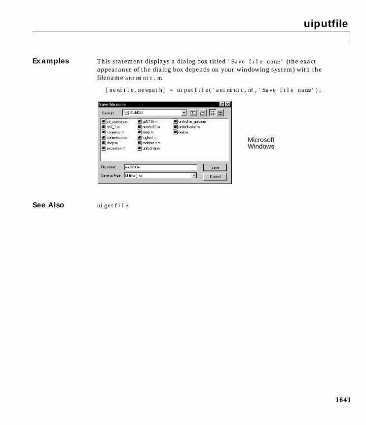
uiputfile
1641
Examples This statement displays a dialog box titled 'Save file name' (the exactappearance of the dialog box depends on your windowing system) with thefilename animinit.m.
[newfile,newpath] = uiputfile('animinit.m','Save file name');
See Also uigetfile
MicrosoftWindows
uiresume, uiwait
1642
1uiresume, uiwaitPurpose Control program execution
Syntax uiwait(h)uiwaituiresume(h)
Description The uiwait and uiresume functions block and resume MATLAB programexecution.
uiwait blocks execution until uiresume is called or the current figure isdeleted. This syntax is the same as uiwait(gcf).
uiwait(h) blocks execution until uiresume is called or the figure h is deleted.
uiresume(h) resumes the M-file execution that uiwait suspended.
Remarks When creating a dialog, you should have a uicontrol with a callback that callsuiresume or a callback that destroys the dialog box. These are the only methodsthat resume program execution after the uiwait function blocks execution.
uiwait is a convenient way to use the waitfor command. You typically use itin conjunction with a dialog box. It provides a way to block the execution of theM-file that created the dialog, until the user responds to the dialog box. Whenused in conjunction with a modal dialog, uiwait/uiresume can block theexecution of the M-file and restrict user interaction to the dialog only.
See Also uicontrol, uimenu, waitfor, figure, dialog
uisetcolor
1643
1uisetcolorPurpose Set an object’s ColorSpec from a dialog box interactively
Syntax c = uisetcolor(h_or_c, 'DialogTitle');
Description uisetcolor displays a dialog box for the user to fill in, then applies the selectedcolor to the appropriate property of the graphics object identified by the firstargument.
h_or_c can be either a handle to a graphics object or an RGB triple. If youspecify a handle, it must specify a graphics object that have a Color property.If you specify a color, it must be a valid RGB triple (e.g., [1 0 0] for red). Thecolor specified is used to initialize the dialog box. If no initial RGB is specified,the dialog box initializes the color to black.
DialogTitle is a string that is used as the title of the dialog box.
c is the RGB value selected by the user. If the user presses Cancel from thedialog box, or if any error occurs, c is set to the input RGB triple, if provided;otherwise, it is set to 0.
See Also ColorSpec
uisetfont
1644
1uisetfontPurpose Modify font characteristics for objects interactively
Syntax uisetfontuisetfont(h)uisetfont(S)uisetfont(h,'DialogTitle')uisetfont(S,'DialogTitle')S = uisetfont(...)
Description uisetfont enables you to change font properties (FontName, FontUnits,FontSize, FontWeight, and FontAngle) for a text, axes, or uicontrol object. Thefunction returns a structure consisting of font properties and values. You canspecify an alternate title for the dialog box.
uisetfont displays the dialog box and returns the selected font properties.
uisetfont(h) displays a dialog box, initializing the font property values withthe values of those properties for the object whose handle is h. Selected fontproperty values are applied to the current object. If a second argument issupplied, it specifies a name for the dialog box.
uisetfont(S) displays a dialog box, initializing the font property values withthe values defined for the specified structure (S). S must define legal values forone or more of these properties: FontName, FontUnits, FontSize, FontWeight,and FontAngle and the field names must match the property names exactly. Ifother properties are defined, they are ignored. If a second argument issupplied, it specifies a name for the dialog box.
uisetfont('DialogTitle') displays a dialog box with the title DialogTitleand returns the values of the font properties selected in the dialog box.
If a left-hand argument is specified, the properties FontName, FontUnits,FontSize, FontWeight, and FontAngle are returned as fields in a structure. Ifthe user presses Cancel from the dialog box or if an error occurs, the outputvalue is set to 0.
uisetfont
1645
Example These statements create a text object, then display a dialog box (labeled UpdateFont) that enables you to change the font characteristics:
h = text(.5,.5,'Figure Annotation');uisetfont(h,'Update Font')
These statements create two push buttons, then set the font properties of onebased on the values set for the other:
% Create push button with string ABCc1 = uicontrol('Style', 'pushbutton', ...
'Position', [10 10 100 20], 'String', 'ABC');% Create push button with string XYZc2 = uicontrol('Style', 'pushbutton', ...
'Position', [10 50 100 20], 'String', 'XYZ');% Display set font dialog box for c1, make selections, save to dd = uisetfont(c1)% Apply those settings to c2set(c2, d)
See Also axes, text, uicontrol
undocheckout
1646
1undocheckoutPurpose Undo previous checkout from source control system
GraphicalInterface
As an alternative to the undocheckout function, use Source Control UndoCheckout in the Editor, Simulink, or Stateflow File menu.
Syntax undocheckout('filename')undocheckout('filename1','filename2','filename3', ...)
Description undocheckout('filename') makes the file filename available for checkout,where filename does not reflect any of the changes you made after you lastchecked it out. filename must be the full pathname for the file.
undocheckout('filename1','filename2','filename3', ...) makes thefilename1 through filenamen available for checkout, where the files do notreflect any of the changes you made after you last checked them out. Use thefull pathnames for the files.
Examples Typing
undocheckout('/matlab/mymfiles/clock.m', ...'/matlab/mymfiles/calendar.m')
undoes the checkouts of /matlab/mymfiles/clock.m and/matlab/mymfiles/calendar.m from the source control system.
See Also checkin, checkout
union
1647
1unionPurpose Set union of two vectors
Syntax c = union(a,b)c = union(A,B,'rows')[c,ia,ib] = union(...)
Description c = union(a,b) returns the combined values from a and b but with norepetitions. The resulting vector is sorted in ascending order. In set theoreticterms, c = a ∪ b. a and b can be cell arrays of strings.
c = union(A,B,'rows') when A and B are matrices with the same number ofcolumns returns the combined rows from A and B with no repetitions.
[c,ia,ib] = union(...) also returns index vectors ia and ib such thatc = a(ia) ∪ b(ib), or for row combinations, c = a(ia,:) ∪ b(ib,:). If avalue appears in both a and b, union indexes its occurence in b. If a valueappears more than once in b or in a (but not in b), union indexes the lastoccurence of the value.
Examples a = [-1 0 2 4 6];b = [-1 0 1 3];[c,ia,ib] = union(a,b);c =
-1 0 1 2 3 4 6
ia =
3 4 5
ib =
1 2 3 4
See Also intersect, setdiff, setxor, unique
unique
1648
1uniquePurpose Unique elements of a vector
Syntax b = unique(a)b = unique(A,'rows')[b,i,j] = unique(...)
Description b = unique(a) returns the same values as in a but with no repetitions. Theresulting vector is sorted in ascending order. a can be a cell array of strings.
b = unique(A,'rows') returns the unique rows of A.
[b,i,j] = unique(...) also returns index vectors i and j such that b = a(i)and a = b(j). Each element of i is the greatest subscript such that b = a(i).For row combinations, b = a(i,:) and a = b(j,:).
Examples a = [1 1 5 6 2 3 3 9 8 6 2 4]a =1 1 5 6 2 3 3 9 8 6 2 4
[b,i,j] = unique(a)b =
1 2 3 4 5 6 8 9i =
2 11 7 12 3 10 9 8j =1 1 5 6 2 3 3 8 7 6 2 4
a(i)ans =
1 2 3 4 5 6 8 9
b(j)ans =1 1 5 6 2 3 3 9 8 6 2 4
See Also intersect, ismember, setdiff, setxor, union
unix
1649
1unixPurpose Execute a UNIX command and return the result
Syntax unix commandstatus = unix('command')[status,result] = unix('command')[status,result] = unix('command','-echo')
Description unix command calls upon the UNIX operating system to execute the givencommand.
status = unix('command') returns completion status to the status variable.
[status, result] = unix('command') returns the standard output to theresult variable, in addition to completion status, .
[status,result] = unix('command','-echo') forces the output to theCommand Window, even though it is also being assigned into a variable.
Examples The following example lists all users that are currently logged in. It returns azero (success) in s and a string containing the list of users in w.
[s,w] = unix('who');
The next example returns a nonzero value in s to indicate failure and returnsan error message in w because why is not a UNIX command.
[s,w] = unix('why')s = 1w =why: Command not found.
When including the -echo flag, MATLAB displays the results of the commandin the Command Window as it executes as well as assigning the results to thereturn variable, w.
[s,w] = unix('who','-echo');
See Also Special Characters
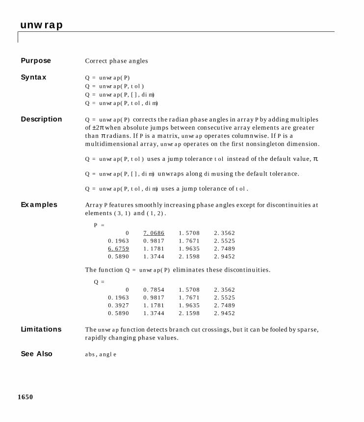
unwrap
1650
1unwrapPurpose Correct phase angles
Syntax Q = unwrap(P)Q = unwrap(P,tol)Q = unwrap(P,[],dim)Q = unwrap(P,tol,dim)
Description Q = unwrap(P) corrects the radian phase angles in array P by adding multiplesof ±2π when absolute jumps between consecutive array elements are greaterthan π radians. If P is a matrix, unwrap operates columnwise. If P is amultidimensional array, unwrap operates on the first nonsingleton dimension.
Q = unwrap(P,tol) uses a jump tolerance tol instead of the default value, π.
Q = unwrap(P,[],dim) unwraps along dim using the default tolerance.
Q = unwrap(P,tol,dim) uses a jump tolerance of tol.
Examples Array P features smoothly increasing phase angles except for discontinuities atelements (3,1) and (1,2).
P = 0 7.0686 1.5708 2.3562 0.1963 0.9817 1.7671 2.5525
6.6759 1.1781 1.9635 2.7489 0.5890 1.3744 2.1598 2.9452
The function Q = unwrap(P) eliminates these discontinuities.
Q = 0 0.7854 1.5708 2.3562 0.1963 0.9817 1.7671 2.5525 0.3927 1.1781 1.9635 2.7489 0.5890 1.3744 2.1598 2.9452
Limitations The unwrap function detects branch cut crossings, but it can be fooled by sparse,rapidly changing phase values.
See Also abs, angle
upper
1651
1upperPurpose Convert string to upper case
Syntax t = upper('str')B = upper(A)
Description t = upper('str') converts any lower-case characters in the string str to thecorresponding upper-case characters and leaves all other charactersunchanged.
B = upper(A) when A is a cell array of strings, returns a cell array the samesize as A containing the result of applying upper to each string within A.
Examples upper('attention!') is ATTENTION!.
Remarks Character sets supported:
• PC: Windows Latin-1
• Other: ISO Latin-1 (ISO 8859-1)
See Also lower
var
1652
1varPurpose Variance
Syntax var(X)var(X,1)var(X,w)
Description var(X) returns the variance of X for vectors. For matrices, var(X)is a rowvector containing the variance of each column of X. var(X) normalizes by N-1where N is the sequence length. This makes var(X) the best unbiased estimateof the variance if X is a sample from a normal distribution.
var(X,1) normalizes by N and produces the second moment of the sampleabout its mean.
var(X,W) computes the variance using the weight vector W. The number ofelements in W must equal the number of rows in X unless W = 1, which is treatedas a short-cut for a vector of ones. The elements of W must be positive. varnormalizes W by dividing each element in W by the sum of all its elements.
The variance is the square of the standard deviation (STD).
See Also corrcoef, cov, std
varargin, varargout
1653
1varargin, varargoutPurpose Pass or return variable numbers of arguments
Syntax function varargout = foo(n)function y = bar(varargin)
Description function varargout = foo(n) returns a variable number of arguments fromfunction foo.m.
function y = bar(varargin) accepts a variable number of arguments intofunction bar.m.
The varargin and varargout statements are used only inside a function M-fileto contain the optional arguments to the function. Each must be declared as thelast argument to a function, collecting all the inputs or outputs from that pointonwards. In the declaration, varargin and varargout must be lowercase.
Examples The function
function myplot(x,varargin)plot(x,varargin:)
collects all the inputs starting with the second input into the variablevarargin. myplot uses the comma-separated list syntax varargin: to passthe optional parameters to plot. The call
myplot(sin(0:.1:1),'color',[.5 .7 .3],'linestyle',':')
results in varargin being a 1-by-4 cell array containing the values 'color',[.5 .7 .3], 'linestyle', and ':'.
The function
function [s,varargout] = mysize(x)nout = max(nargout,1)-1;s = size(x);for i=1:nout, varargout(i) = s(i); end
returns the size vector and, optionally, individual sizes. So
[s,rows,cols] = mysize(rand(4,5));
returns s = [4 5], rows = 4, cols = 5.
varargin, varargout
1654
See Also nargin , nargout, nargchk
vectorize
1655
1vectorizePurpose Vectorize expression
Syntax vectorize(string)vectorize(function)
Description vectorize(string) inserts a . before any ^, * or / in string. The result is acharacter string.
vectorize(function) when function is an inline function object, vectorizesthe formula for function. The result is the vectorized version of the inlinefunction.
See Also inline
cd, dbtype, delete, dir, partialpath, path, what, who
ver
1656
1verPurpose Display version information for MATLAB, Simulink, and toolboxes
GraphicalInterface
As an alternative to the ver function, select About from the Help menu in anyproduct that has a Help menu.
Syntax verver toolboxv = ver('toolbox')
Description ver displays the current version numbers and release dates for MATLAB,Simulink, and all toolboxes.
ver toolbox displays the current version number and release date for thetoolbox specified by toolbox. The name, toolbox, corresponds to the directoryname that holds the Contents.m file for that toolbox. For example, Contents.mfor the Fuzzy Logic Toolbox resides in the fuzzy directory. You therefore usever fuzzy to obtain the version of this toolbox.
v = ver('toolbox') returns the version information in structure array, v,having fields Name, Version, Release, and Date.
Remarks See comments near the top of ver.m for information on how your own toolboxescan use the ver function. Type the following at the MATLAB command prompt.
type ver.m
Examples To return version information for the Fuzzy Logic Toolbox,
ver fuzzyFuzzy Logic Toolbox Version 2.0.1 (R11) 16-Sep-1998
To return version information for MATLAB in a structure array, v,
v = ver('matlab')v = Name: 'MATLAB Toolbox' Version: '6.0' Release: '(R12)' Date: '30-Dec-1999'

ver
1657
See Also help, version, whatsnew
Also, type help info at the Command Window prompt.
version
1658
1versionPurpose Get MATLAB version number
GraphicalInterface
As an alternative to the version function, select About from the Help menu inthe MATLAB desktop.
Syntax versionversion -javav = version[v,d] = version
Description version displays the MATLAB version number.
version -java displays the version of the Java VM used by MATLAB.
v = version returns a string v containing the MATLAB version number.
[v,d] = version also returns a string d containing the date of the version.
Examples [v,d]=version
v =6.0.0.60356 (R12)
d =May 2 2000
See Also help, ver, whatsnew
Also, type help info at the Command Window prompt.
view
1659
1viewPurpose Viewpoint specification
Syntax view(az,el)view([az,el])view([x,y,z])view(2)view(3)view(T)
[az,el] = viewT = view
Description The position of the viewer (the viewpoint) determines the orientation of theaxes. You specify the viewpoint in terms of azimuth and elevation, or by a pointin three-dimensional space.
view(az,el) and view([az,el]) set the viewing angle for athree-dimensional plot. The azimuth, az, is the horizontal rotation about thez-axis as measured in degrees from the negative y-axis. Positive values indicatecounterclockwise rotation of the viewpoint. el is the vertical elevation of theviewpoint in degrees. Positive values of elevation correspond to moving abovethe object; negative values correspond to moving below the object.
view([x,y,z]) sets the viewpoint to the Cartesian coordinates x, y, and z. Themagnitude of (x,y,z) is ignored.
view(2) sets the default two-dimensional view, az = 0, el = 90.
view(3) sets the default three-dimensional view, az = –37.5, el = 30.
view(T) sets the view according to the transformation matrix T, which is a4-by-4 matrix such as a perspective transformation generated by viewmtx.
[az,el] = view returns the current azimuth and elevation.
T = view returns the current 4-by-4 transformation matrix.
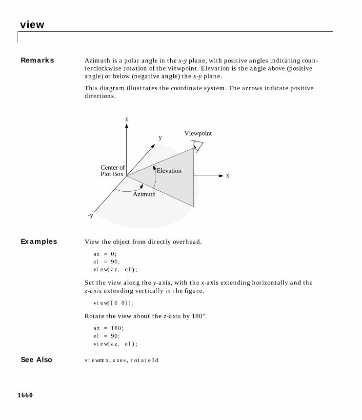
view
1660
Remarks Azimuth is a polar angle in the x-y plane, with positive angles indicating coun-terclockwise rotation of the viewpoint. Elevation is the angle above (positiveangle) or below (negative angle) the x-y plane.
This diagram illustrates the coordinate system. The arrows indicate positivedirections.
Examples View the object from directly overhead.
az = 0;el = 90;view(az, el);
Set the view along the y-axis, with the x-axis extending horizontally and thez-axis extending vertically in the figure.
view([0 0]);
Rotate the view about the z-axis by 180°.
az = 180;el = 90;view(az, el);
See Also viewmtx, axes, rotate3d
Center of
Viewpoint
z
x
y
Azimuth
Elevation
-y
Plot Box
view
1661
axes graphics object properties: CameraPosition, CameraTarget,CameraViewAngle, Projection.
viewmtx
1662
1viewmtxPurpose View transformation matrices
Syntax T = viewmtx(az,el)T = viewmtx(az,el,phi)T = viewmtx(az,el,phi,xc)
Description viewmtx computes a 4-by-4 orthographic or perspective transformation matrixthat projects four-dimensional homogeneous vectors onto a two-dimensionalview surface (e.g., your computer screen).
T = viewmtx(az,el) returns an orthographic transformation matrixcorresponding to azimuth az and elevation el. az is the azimuth (i.e.,horizontal rotation) of the viewpoint in degrees. el is the elevation of theviewpoint in degrees. This returns the same matrix as the commands
view(az,el)T = view
but does not change the current view.
T = viewmtx(az,el,phi) returns a perspective transformation matrix. phi isthe perspective viewing angle in degrees. phi is the subtended view angle of thenormalized plot cube (in degrees) and controls the amount of perspectivedistortion.
You can use the matrix returned to set the view transformation with view(T).The 4-by-4 perspective transformation matrix transforms four-dimensionalhomogeneous vectors into unnormalized vectors of the form (x,y,z,w), where w isnot equal to 1. The x- and y-components of the normalized vector (x/w, y/w, z/w,1) are the desired two-dimensional components (see example below).
Phi Description
0 degrees Orthographic projection
10 degrees Similar to telephoto lens
25 degrees Similar to normal lens
60 degrees Similar to wide angle lens
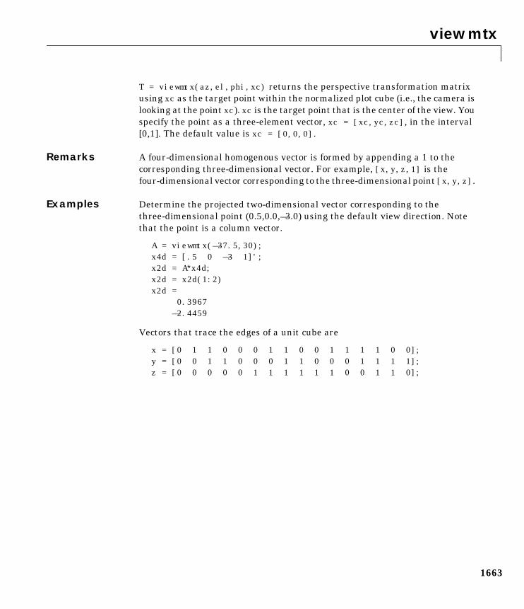
viewmtx
1663
T = viewmtx(az,el,phi,xc) returns the perspective transformation matrixusing xc as the target point within the normalized plot cube (i.e., the camera islooking at the point xc). xc is the target point that is the center of the view. Youspecify the point as a three-element vector, xc = [xc,yc,zc], in the interval[0,1]. The default value is xc = [0,0,0].
Remarks A four-dimensional homogenous vector is formed by appending a 1 to thecorresponding three-dimensional vector. For example, [x,y,z,1] is thefour-dimensional vector corresponding to the three-dimensional point [x,y,z].
Examples Determine the projected two-dimensional vector corresponding to thethree-dimensional point (0.5,0.0,—3.0) using the default view direction. Notethat the point is a column vector.
A = viewmtx(—37.5,30);x4d = [.5 0 —3 1]';x2d = A∗x4d;x2d = x2d(1:2)x2d =
0.3967—2.4459
Vectors that trace the edges of a unit cube are
x = [0 1 1 0 0 0 1 1 0 0 1 1 1 1 0 0];y = [0 0 1 1 0 0 0 1 1 0 0 0 1 1 1 1];z = [0 0 0 0 0 1 1 1 1 1 1 0 0 1 1 0];
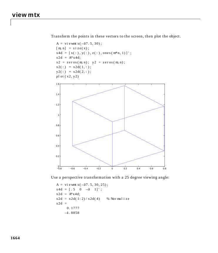
viewmtx
1664
Transform the points in these vectors to the screen, then plot the object.
A = viewmtx(—37.5,30);[m,n] = size(x);x4d = [x(:),y(:),z(:),ones(m*n,1)]';x2d = A*x4d;x2 = zeros(m,n); y2 = zeros(m,n);x2(:) = x2d(1,:);y2(:) = x2d(2,:);plot(x2,y2)
Use a perspective transformation with a 25 degree viewing angle:
A = viewmtx(—37.5,30,25);x4d = [.5 0 —3 1]';x2d = A∗x4d;x2d = x2d(1:2)/x2d(4) % Normalizex2d =
0.1777—1.8858
−0.8 −0.6 −0.4 −0.2 0 0.2 0.4 0.6 0.80
0.2
0.4
0.6
0.8
1
1.2
1.4
1.6
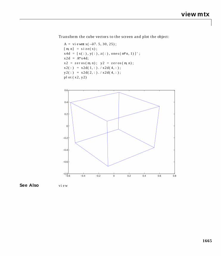
viewmtx
1665
Transform the cube vectors to the screen and plot the object:
A = viewmtx(—37.5,30,25);[m,n] = size(x);x4d = [x(:),y(:),z(:),ones(m*n,1)]';x2d = A*x4d;x2 = zeros(m,n); y2 = zeros(m,n);x2(:) = x2d(1,:)./x2d(4,:);y2(:) = x2d(2,:)./x2d(4,:);plot(x2,y2)
See Also view
−0.6 −0.4 −0.2 0 0.2 0.4 0.6 0.8−0.8
−0.6
−0.4
−0.2
0
0.2
0.4
0.6
volumebounds
1666
1volumeboundsPurpose Returns coordinate and color limits for volume data
Syntax lims = volumebounds(X,Y,Z,V)lims = volumebounds(X,Y,Z,U,V,W)lims = volumebounds(V), lims = volumebounds(U,V,W)
Description lims = volumebounds(X,Y,Z,V) returns the x,y,z and color limits of thecurrent axes for scalar data. lims is returned as a vector:
[xmin xmax ymin ymax zmin zmax cmin cmax]
You can pass this vector to the axis command.
lims = volumebounds(X,Y,Z,U,V,W) returns the x, y, and z limits of thecurrent axes for vector data. lims is returned as a vector:
[xmin xmax ymin ymax zmin zmax]
lims = volumebounds(V), lims = volumebounds(U,V,W) assumes X, Y, andZ are determined by the expression:
[X Y Z] = meshgrid(1:n,1:m,1:p)
where [m n p] = size(V).
Examples This example uses volumebounds to set the axis and color limits for anisosurface generated by the flow function.
[x y z v] = flow;p = patch(isosurface(x,y,z,v,-3));isonormals(x,y,z,v,p)daspect([1 1 1])isocolors(x,y,z,flipdim(v,2),p)shading interpaxis(volumebounds(x,y,z,v))view(3)camlightlighting phong
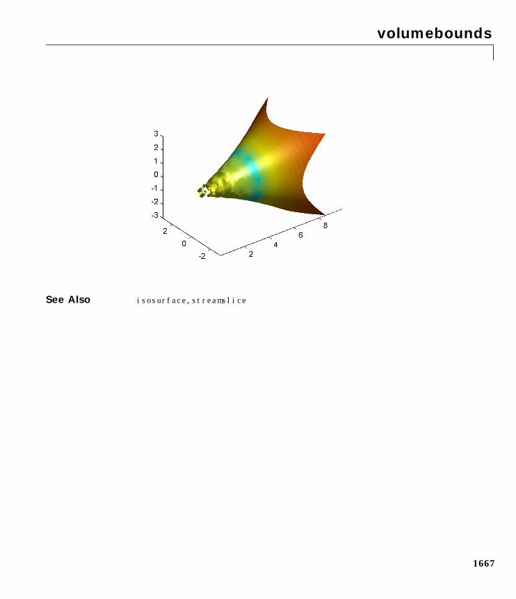
volumebounds
1667
See Also isosurface, streamslice
voronoi
1668
1voronoiPurpose Voronoi diagram
Syntax voronoi(x,y)voronoi(x,y,TRI)h = voronoi(...,'LineSpec')[vx,vy] = voronoi(...)
Definition Consider a set of coplanar points For each point in the set you candraw a boundary enclosing all the intermediate points lying closer to thanto other points in the set Such a boundary is called a Voronoi polygon, andthe set of all Voronoi polygons for a given point set is called a Voronoi diagram.
Description voronoi(x,y) plots the Voronoi diagram for the points x,y.
voronoi(x,y,TRI) uses the triangulation TRI instead of computing it viadelaunay.
h = voronoi(...,'LineSpec') plots the diagram with color and line stylespecified and returns handles to the line objects created in h.
[vx,vy] = voronoi(...) returns the vertices of the Voronoi edges in vx andvy so that plot(vx,vy,'-',x,y,'.') creates the Voronoi diagram.
Examples This code plots the Voronoi diagram for 10 randomly generated points.
rand('state',0);x = rand(1,10); y = rand(1,10);[vx, vy] = voronoi(x,y);plot(x,y,'r+',vx,vy,'b-'); axis equal
P. Px P,Px
P.
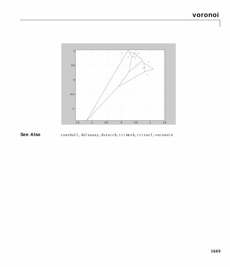
voronoi
1669
See Also convhull, delaunay, dsearch, trimesh, trisurf, voronoin
-1.5 -1 -0.5 0 0.5 1 1.5
-1
-0.5
0
0.5
1
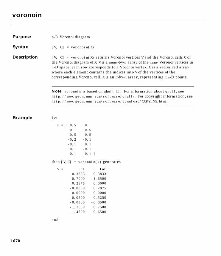
voronoin
1670
1voronoinPurpose n-D Voronoi diagram
Syntax [V, C] = voronoin(X)
Description [V, C] = voronoin(X) returns Voronoi vertices V and the Voronoi cells C ofthe Voronoi diagram of X. V is a numv-by-n array of the numv Voronoi vertices inn-D space, each row corresponds to a Voronoi vertex. C is a vector cell arraywhere each element contains the indices into V of the vertices of thecorresponding Voronoi cell. X is an m-by-n array, representing m n-D points.
Note voronoin is based on qhull [1]. For information about qhull, seehttp://www.geom.umn.edu/software/qhull/. For copyright information, seehttp://www.geom.umn.edu/software/download/COPYING.html.
Example Let
x = [ 0.5 0 0 0.5 -0.5 -0.5 -0.2 -0.1 -0.1 0.1 0.1 -0.1 0.1 0.1 ]
then [V,C] = voronoin(x) generates
V = Inf Inf 0.3833 0.3833 0.7000 -1.6500 0.2875 0.0000 -0.0000 0.2875 -0.0000 -0.0000 -0.0500 -0.5250 -0.0500 -0.0500 -1.7500 0.7500 -1.4500 0.6500
and
voronoin
1671
C: = 4 2 1 3 10 5 2 1 9 9 1 3 7 10 8 7 9 10 5 6 8 8 6 4 3 7 6 4 2 5
In particular, the fifth Voronoi cell consists of 4 points: V(10,:), V(5,:),V(6,:), V(8,:).
See Also convhulln, delaunayn, voronoi
Reference [1] National Science and Technology Research Center for Computation andVisualization of Geometric Structures (The Geometry Center), University ofMinnesota. 1993.
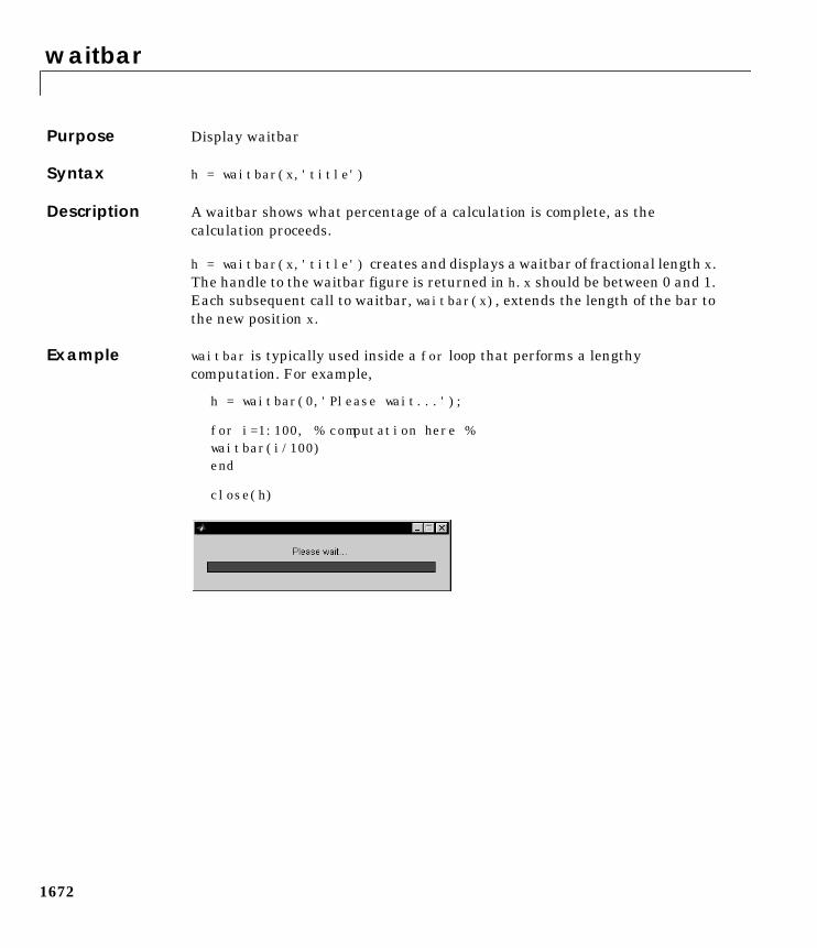
waitbar
1672
1waitbarPurpose Display waitbar
Syntax h = waitbar(x,'title')
Description A waitbar shows what percentage of a calculation is complete, as thecalculation proceeds.
h = waitbar(x,'title') creates and displays a waitbar of fractional length x.The handle to the waitbar figure is returned in h. x should be between 0 and 1.Each subsequent call to waitbar, waitbar(x), extends the length of the bar tothe new position x.
Example waitbar is typically used inside a for loop that performs a lengthycomputation. For example,
h = waitbar(0,'Please wait...');
for i=1:100, % computation here %waitbar(i/100)end
close(h)
waitfor
1673
1waitforPurpose Wait for condition
Syntax waitfor(h)waitfor(h,'PropertyName')waitfor(h,'PropertyName',PropertyValue)
Description The waitfor function blocks the caller’s execution stream so thatcommand-line expressions, callbacks, and statements in the blocked M-file donot execute until a specified condition is satisfied.
waitfor(h) returns when the graphics object identified by h is deleted or whena Ctrl-C is typed in the Command Window. If h does not exist, waitfor returnsimmediately without processing any events.
waitfor(h,'PropertyName'), in addition to the conditions in the previoussyntax, returns when the value of 'PropertyName' for the graphics object hchanges. If 'PropertyName' is not a valid property for the object, waitforreturns immediately without processing any events.
waitfor(h,'PropertyName',PropertyValue), in addition to the conditions inthe previous syntax, waitfor returns when the value of 'PropertyName' forthe graphics object h changes to PropertyValue. waitfor returns immediatelywithout processing any events if 'PropertyName' is set to PropertyValue.
Remarks While waitfor blocks an execution stream, other execution streams in the formof callbacks may execute as a result of various events (e.g., pressing a mousebutton).
waitfor can block nested execution streams. For example, a callback invokedduring a waitfor statement can itself invoke waitfor.
See Also uiresume, uiwait
waitforbuttonpress
1674
1waitforbuttonpressPurpose Wait for key or mouse button press
Syntax k = waitforbuttonpress
Description k = waitforbuttonpress blocks the caller’s execution stream until thefunction detects that the user has pressed a mouse button or a key while thefigure window is active. The function returns
• 0 if it detects a mouse button press
• 1 if it detects a key press
Additional information about the event that causes execution to resume isavailable through the figure’s CurrentCharacter, SelectionType, andCurrentPoint properties.
If a WindowButtonDownFcn is defined for the figure, its callback is executedbefore waitforbuttonpress returns a value.
Example These statements display text in the Command Window when the user eitherclicks a mouse button or types a key in the figure window:
w = waitforbuttonpress;if w == 0
disp('Button press')else
disp('Key press')end
See Also dragrect, figure, gcf, ginput, rbbox, waitfor
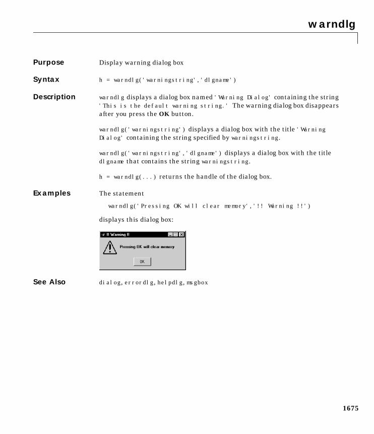
warndlg
1675
1warndlgPurpose Display warning dialog box
Syntax h = warndlg('warningstring','dlgname')
Description warndlg displays a dialog box named 'Warning Dialog' containing the string'This is the default warning string.' The warning dialog box disappearsafter you press the OK button.
warndlg('warningstring') displays a dialog box with the title 'WarningDialog' containing the string specified by warningstring.
warndlg('warningstring','dlgname') displays a dialog box with the titledlgname that contains the string warningstring.
h = warndlg(...) returns the handle of the dialog box.
Examples The statement
warndlg('Pressing OK will clear memory','!! Warning !!')
displays this dialog box:
See Also dialog, errordlg, helpdlg, msgbox
warning
1676
1warningPurpose Display warning message
Syntax warning('message')warning onwarning offwarning backtracewarning debugwarning oncewarning always[s,f] = warning
Description warning('message') displays the text 'message' as does the disp function,except that with warning, message display can be suppressed.
warning off suppresses all subsequent warning messages.
warning on re-enables them.
warning backtrace is the same as warning on except that the file and linenumber that produced the warning are displayed.
warning debug is the same as dbstop if warning and triggers the debuggerwhen a warning is encountered.
warning once displays Handle Graphics backwards compatibility warningsonly once per session.
warning always displays Handle Graphics backwards compatibility warningsas they are encountered (subject to current warning state).
[s,f] = warning returns the current warning state s and the current warningfrequency f as strings.
Remarks Use dbstop on warning to trigger the debugger when a warning isencountered.
See Also dbstop, disp, error, errordlg
waterfall
1677
1waterfallPurpose Waterfall plot
Syntax waterfall(Z)waterfall(X,Y,Z)waterfall(...,C)
h = waterfall(...)
Description The waterfall function draws a mesh similar to the meshz function, but it doesnot generate lines from the columns of the matrices. This produces a“waterfall” effect.
waterfall(Z) creates a waterfall plot using x = 1:size(Z,1) andy = 1:size(Z,1). Z determines the color, so color is proportional to surfaceheight.
waterfall(X,Y,Z) creates a waterfall plot using the values specified in X, Y,and Z. Z also determines the color, so color is proportional to the surface height.If X and Y are vectors, X corresponds to the columns of Z, and Y corresponds tothe rows, where length(x) = n, length(y) = m, and [m,n] = size(Z). X andY are vectors or matrices that define the x and y coordinates of the plot. Z is amatrix that defines the z coordinates of the plot (i.e., height above a plane). IfC is omitted, color is proportional to Z.
waterfall(...,C) uses scaled color values to obtain colors from the currentcolormap. Color scaling is determined by the range of C, which must be thesame size as Z. MATLAB performs a linear transformation on C to obtain colorsfrom the current colormap.
h = waterfall(...) returns the handle of the patch graphics object used todraw the plot.
Remarks For column-oriented data analysis, use waterfall(Z') orwaterfall(X',Y',Z').
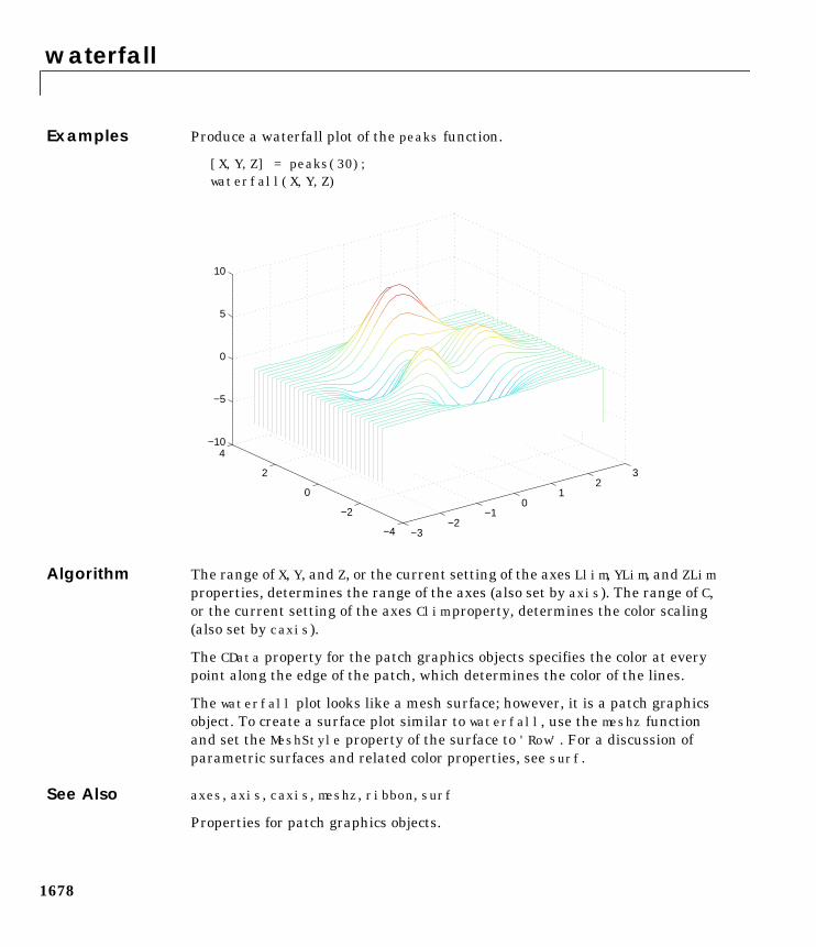
waterfall
1678
Examples Produce a waterfall plot of the peaks function.
[X,Y,Z] = peaks(30);waterfall(X,Y,Z)
Algorithm The range of X, Y, and Z, or the current setting of the axes Llim, YLim, and ZLimproperties, determines the range of the axes (also set by axis). The range of C,or the current setting of the axes Clim property, determines the color scaling(also set by caxis).
The CData property for the patch graphics objects specifies the color at everypoint along the edge of the patch, which determines the color of the lines.
The waterfall plot looks like a mesh surface; however, it is a patch graphicsobject. To create a surface plot similar to waterfall, use the meshz functionand set the MeshStyle property of the surface to 'Row'. For a discussion ofparametric surfaces and related color properties, see surf.
See Also axes, axis, caxis, meshz, ribbon, surf
Properties for patch graphics objects.
−3−2
−10
12
3
−4
−2
0
2
4−10
−5
0
5
10
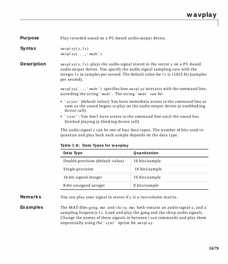
wavplay
1679
1wavplayPurpose Play recorded sound on a PC-based audio output device.
Syntax wavplay(y,fs)wavplay(...,'mode')
Description wavplay(y,fs) plays the audio signal stored in the vector y on a PC-basedaudio output device. You specify the audio signal sampling rate with theinteger fs in samples per second. The default value for fs is 11025 Hz (samplesper second).
wavplay(...,'mode') specifies how wavplay interacts with the command line,according the string 'mode'. The string 'mode' can be:
• 'async' (default value): You have immediate access to the command line assoon as the sound begins to play on the audio output device (a nonblockingdevice call).
• 'sync': You don’t have access to the command line until the sound hasfinished playing (a blocking device call).
The audio signal y can be one of four data types. The number of bits used toquantize and play back each sample depends on the data type.
Remarks You can play your signal in stereo if y is a two-column matrix.
Examples The MAT-files gong.mat and chirp.mat both contain an audio signal y, and asampling frequency fs. Load and play the gong and the chirp audio signals.Change the names of these signals in between load commands and play themsequentially using the 'sync' option for wavplay.
Table 1-8: Data Types for wavplay
Data Type Quantization
Double-precision (default value) 16 bits/sample
Single-precision 16 bits/sample
16-bit signed integer 16 bits/sample
8-bit unsigned integer 8 bits/sample
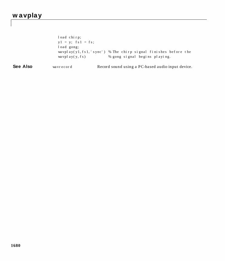
wavplay
1680
load chirp;y1 = y; fs1 = fs;load gong;wavplay(y1,fs1,'sync') % The chirp signal finishes before thewavplay(y,fs) % gong signal begins playing.
See Also wavrecord Record sound using a PC-based audio input device.
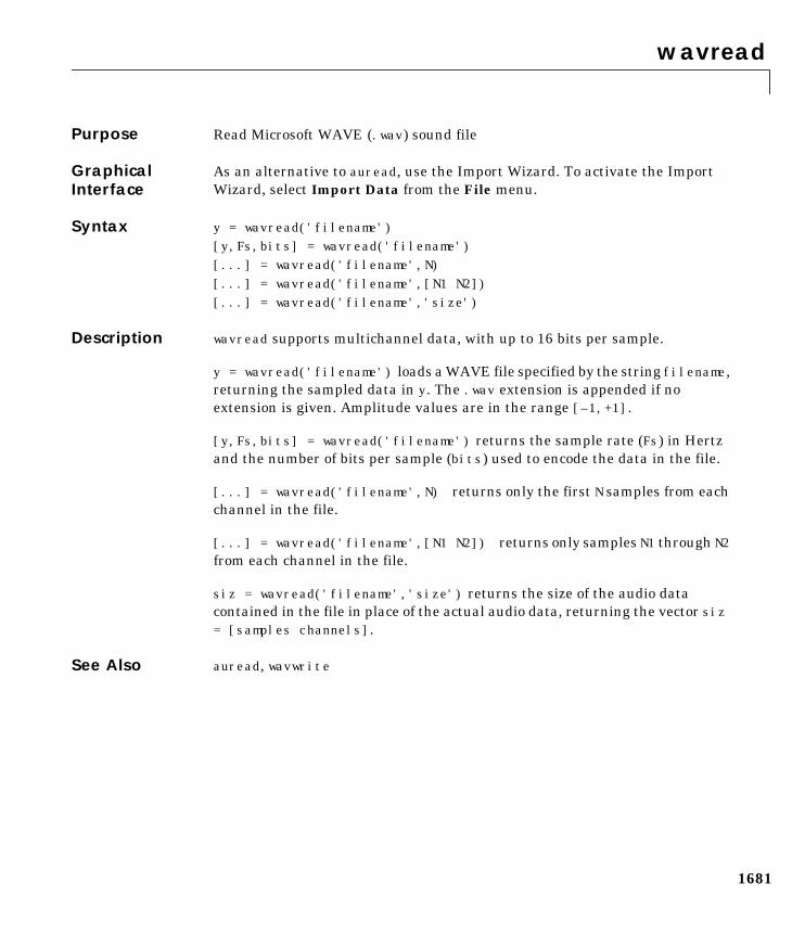
wavread
1681
1wavreadPurpose Read Microsoft WAVE (.wav) sound file
GraphicalInterface
As an alternative to auread, use the Import Wizard. To activate the ImportWizard, select Import Data from the File menu.
Syntax y = wavread('filename')[y,Fs,bits] = wavread('filename')[...] = wavread('filename',N)[...] = wavread('filename',[N1 N2])[...] = wavread('filename','size')
Description wavread supports multichannel data, with up to 16 bits per sample.
y = wavread('filename') loads a WAVE file specified by the string filename,returning the sampled data in y. The .wav extension is appended if noextension is given. Amplitude values are in the range [–1,+1].
[y,Fs,bits] = wavread('filename') returns the sample rate (Fs) in Hertzand the number of bits per sample (bits) used to encode the data in the file.
[...] = wavread('filename',N) returns only the first N samples from eachchannel in the file.
[...] = wavread('filename',[N1 N2]) returns only samples N1 through N2from each channel in the file.
siz = wavread('filename','size') returns the size of the audio datacontained in the file in place of the actual audio data, returning the vector siz= [samples channels].
See Also auread, wavwrite
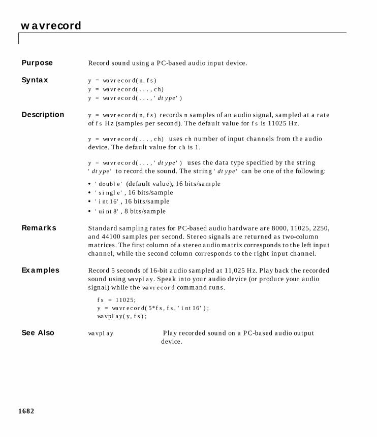
wavrecord
1682
1wavrecordPurpose Record sound using a PC-based audio input device.
Syntax y = wavrecord(n,fs)y = wavrecord(...,ch)y = wavrecord(...,'dtype')
Description y = wavrecord(n,fs) records n samples of an audio signal, sampled at a rateof fs Hz (samples per second). The default value for fs is 11025 Hz.
y = wavrecord(...,ch) uses ch number of input channels from the audiodevice. The default value for ch is 1.
y = wavrecord(...,'dtype') uses the data type specified by the string'dtype' to record the sound. The string 'dtype' can be one of the following:
• 'double' (default value), 16 bits/sample• 'single', 16 bits/sample• 'int16', 16 bits/sample• 'uint8', 8 bits/sample
Remarks Standard sampling rates for PC-based audio hardware are 8000, 11025, 2250,and 44100 samples per second. Stereo signals are returned as two-columnmatrices. The first column of a stereo audio matrix corresponds to the left inputchannel, while the second column corresponds to the right input channel.
Examples Record 5 seconds of 16-bit audio sampled at 11,025 Hz. Play back the recordedsound using wavplay. Speak into your audio device (or produce your audiosignal) while the wavrecord command runs.
fs = 11025;y = wavrecord(5*fs,fs,'int16');wavplay(y,fs);
See Also wavplay Play recorded sound on a PC-based audio outputdevice.
wavwrite
1683
1wavwritePurpose Write Microsoft WAVE (.wav) sound file
Syntax wavwrite(y,'filename')wavwrite(y,Fs,'filename')wavwrite(y,Fs,N,'filename')
Description wavwrite supports multi-channel 8- or 16-bit WAVE data.
wavwrite(y,'filename') writes a WAVE file specified by the string filename.The data should be arranged with one channel per column. Amplitude valuesoutside the range [–1,+1] are clipped prior to writing.
wavwrite(y,Fs,'filename') specifies the sample rate Fs, in Hertz, of thedata.
wavwrite(y,Fs,N,'filename') forces an N-bit file format to be written, whereN <= 16.
See Also auwrite, wavread
web
1684
1webPurpose Point Help browser or Web browser at file or Web site
GraphicalInterface
As an alternative to the web function, type the URL in the page title field at thetop of the display pane in the Help browser.
Syntax web urlweb url -browserstat = web('url', '-browser')
Description web url displays the MATLAB Help browser, loads the file or Web sitespecified by url (Uniform Resource Locator) in it, and returns the status to theCommand Window. Generally, url specifies a local file or a Web site on theInternet. You must specify the full URL. For example, use http://www.mathworks.com instead of www.mathworks.com.
web url -browser displays the default Web browser for your system, loads thefile or Web site specified by url (Uniform Resource Locator) in it, and returnsthe status to the Command Window. Generally, url specifies a local file or aWeb site on the Internet. The URL can be in any form that the browser supports.On Windows, the default Web browser is determined by the operating system.On UNIX, the Web browser used is specified in docopt, in the doccmd string.
stat = web('url', '-browser') is the function form and returns the statusof web to the variable stat.
Examples web file:/disk/dir1/dir2/foo.html points the Help browser to the filefoo.html. If the file is on the MATLAB path, web(['file:'which('foo.html')]) also works.
web http://www.mathworks.com loads The MathWorks Web page into theHelp browser.
Value of status Description
0 Browser was found and launched.
1 Browser was not found.
2 Browser was found but could not be launched.

web
1685
web www.mathworks.com -browser loads The MathWorks Web page into yoursystem’s default Web browser, for example, Netscape Navigator.
Use web mailto:email_address to use your default e-mail application to senda message to email_address.
See Also doc, docopt, helpbrowser
weekday
1686
1weekdayPurpose Day of the week
Syntax [N,S] = weekday(D)
Description [N,S] = weekday(D) returns the day of the week in numeric (N) and string (S)form for each element of a serial date number array or date string. The days ofthe week are assigned these numbers and abbreviations:
Examples Either
[n,s] = weekday(728647)
or
[n,s] = weekday('19-Dec-1994')
returns n = 2 and s = Mon.
See Also datenum, datevec, eomday
N S N S
1 Sun 5 Thu
2 Mon 6 Fri
3 Tue 7 Sat
4 Wed
what
1687
1whatPurpose List MATLAB-specific files in current directory
GraphicalInterface
As an alternative to the what function, use the Current Directory browser. Toopen it, select Current Directory from the View menu in the MATLABdesktop.
Syntax whatwhat dirnames = what('dirname')
Description what lists the M, MAT, MEX, MDL, and P-files and the class directories that residein the current working directory.
what dirname lists the files in directory dirname on the MATLAB search path.It is not necessary to enter the full pathname of the directory. The lastcomponent, or last couple of components, is sufficient.
Use what class to list the files in method directory, @class. For example, whatcfit lists the MATLAB files in toolbox\curvefit\curvefit\@cfit.
s = what('dirname') returns the results in a structure array with thesefields.
what dirname is the unquoted form of the syntax.
Field Description
path Path to directory
m Cell array of M-file names
mat Cell array of MAT-file names
mex Cell array of MEX-file names
mdl Cell array of MDL-file names
p Cell array of P-file names
classes Cell array of class names
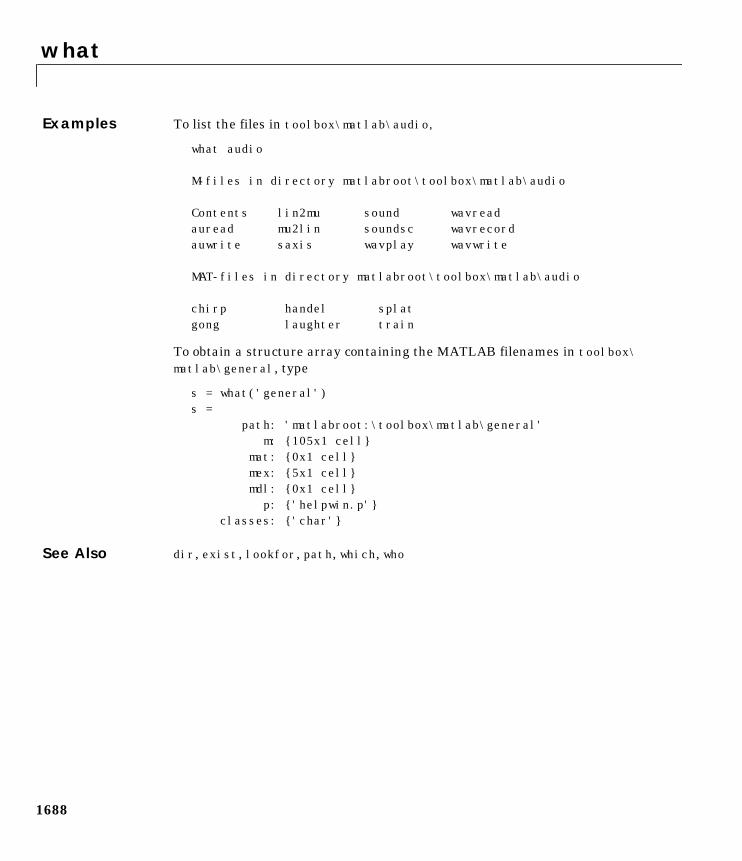
what
1688
Examples To list the files in toolbox\matlab\audio,
what audio
M-files in directory matlabroot\toolbox\matlab\audio
Contents lin2mu sound wavreadauread mu2lin soundsc wavrecordauwrite saxis wavplay wavwrite
MAT-files in directory matlabroot\toolbox\matlab\audio
chirp handel splatgong laughter train
To obtain a structure array containing the MATLAB filenames in toolbox\matlab\general, type
s = what('general')s = path: 'matlabroot:\toolbox\matlab\general' m: 105x1 cell mat: 0x1 cell mex: 5x1 cell mdl: 0x1 cell p: 'helpwin.p' classes: 'char'
See Also dir, exist, lookfor, path, which, who
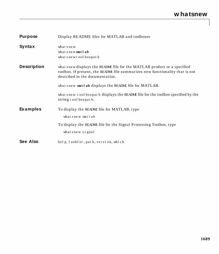
whatsnew
1689
1whatsnewPurpose Display README files for MATLAB and toolboxes
Syntax whatsnewwhatsnew matlabwhatsnew toolboxpath
Description whatsnew displays the README file for the MATLAB product or a specifiedtoolbox. If present, the README file summarizes new functionality that is notdescribed in the documentation.
whatsnew matlab displays the README file for MATLAB.
whatsnew toolboxpath displays the README file for the toolbox specified by thestring toolboxpath.
Examples To display the README file for MATLAB, type
whatsnew matlab
To display the README file for the Signal Processing Toolbox, type
whatsnew signal
See Also help, lookfor, path, version, which
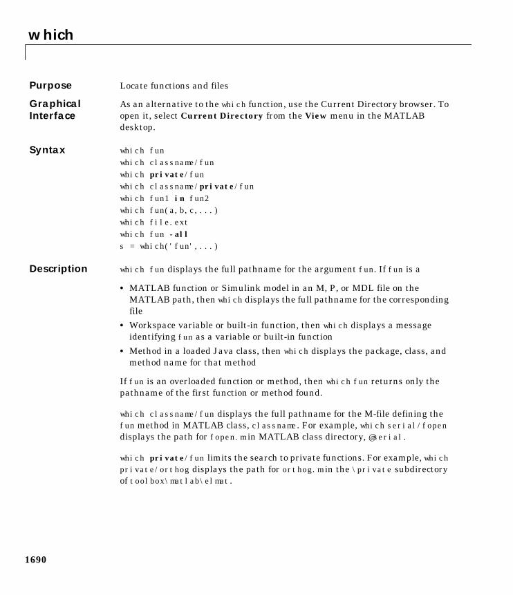
which
1690
1whichPurpose Locate functions and files
GraphicalInterface
As an alternative to the which function, use the Current Directory browser. Toopen it, select Current Directory from the View menu in the MATLABdesktop.
Syntax which funwhich classname/funwhich private/funwhich classname/private/funwhich fun1 in fun2which fun(a,b,c,...)which file.extwhich fun -alls = which('fun',...)
Description which fun displays the full pathname for the argument fun. If fun is a
• MATLAB function or Simulink model in an M, P, or MDL file on theMATLAB path, then which displays the full pathname for the correspondingfile
• Workspace variable or built-in function, then which displays a messageidentifying fun as a variable or built-in function
• Method in a loaded Java class, then which displays the package, class, andmethod name for that method
If fun is an overloaded function or method, then which fun returns only thepathname of the first function or method found.
which classname/fun displays the full pathname for the M-file defining thefun method in MATLAB class, classname. For example, which serial/fopendisplays the path for fopen.m in MATLAB class directory, @serial.
which private/fun limits the search to private functions. For example, whichprivate/orthog displays the path for orthog.m in the \private subdirectoryof toolbox\matlab\elmat.
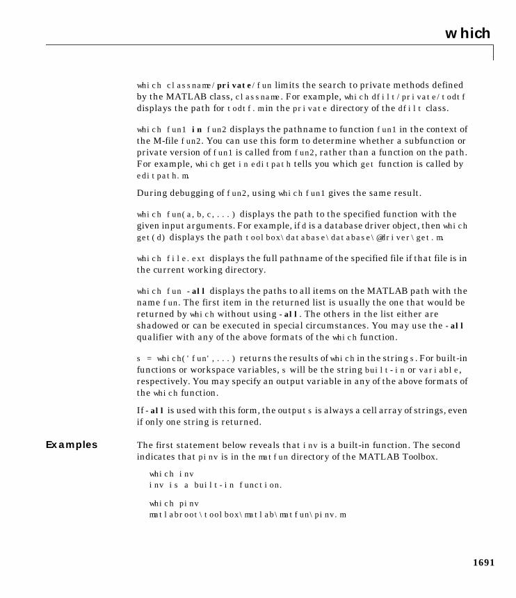
which
1691
which classname/private/fun limits the search to private methods definedby the MATLAB class, classname. For example, which dfilt/private/todtfdisplays the path for todtf.m in the private directory of the dfilt class.
which fun1 in fun2 displays the pathname to function fun1 in the context ofthe M-file fun2. You can use this form to determine whether a subfunction orprivate version of fun1 is called from fun2, rather than a function on the path.For example, which get in editpath tells you which get function is called byeditpath.m.
During debugging of fun2, using which fun1 gives the same result.
which fun(a,b,c,...) displays the path to the specified function with thegiven input arguments. For example, if d is a database driver object, then whichget(d) displays the path toolbox\database\database\@driver\get.m.
which file.ext displays the full pathname of the specified file if that file is inthe current working directory.
which fun -all displays the paths to all items on the MATLAB path with thename fun. The first item in the returned list is usually the one that would bereturned by which without using -all. The others in the list either areshadowed or can be executed in special circumstances. You may use the -allqualifier with any of the above formats of the which function.
s = which('fun',...) returns the results of which in the string s. For built-infunctions or workspace variables, s will be the string built-in or variable,respectively. You may specify an output variable in any of the above formats ofthe which function.
If -all is used with this form, the output s is always a cell array of strings, evenif only one string is returned.
Examples The first statement below reveals that inv is a built-in function. The secondindicates that pinv is in the matfun directory of the MATLAB Toolbox.
which invinv is a built-in function.
which pinvmatlabroot\toolbox\matlab\matfun\pinv.m
which
1692
To find the fopen function used on MATLAB serial class objects
which serial/fopenmatlabroot\toolbox\matlab\iofun\@serial\fopen.m % serial method
To find the setTitle method used on objects of the Java Frame class, the classmust first be loaded into MATLAB. The class is loaded when you create aninstance of the class.
frameObj = java.awt.Frame;
which setTitlejava.awt.Frame.setTitle % Frame method
The following example uses the form, which fun(a,b,c,...). The responsereturned from which depends upon the arguments of the function feval. Whenfun is a function handle, MATLAB evaluates the function using the fevalbuilt-in.
fun = @abs;which feval(fun,-2.5)feval is a built-in function.
When fun is the inline function, MATLAB evaluates the function using thefeval method of the inline class.
fun = inline('abs(x)');which feval(fun,-2.5)matlabroot\toolbox\matlab\funfun\@inline\feval.m % inline method
When you specify an output variable, which returns a cell array of strings tothe variable. You must use the function form of which, enclosing all argumentsin parentheses and single quotes.
s = which('private/stradd','-all');whos s Name Size Bytes Class s 3x1 562 cell arrayGrand total is 146 elements using 562 bytes
See Also dir, doc, exist, lookfor, path, type, what, who
while
1693
1whilePurpose Repeat statements an indefinite number of times
Syntax while expressionstatements
end
Description while repeats statements an indefinite number of times. The statements areexecuted while the real part of expression has all nonzero elements.expression is usually of the form
expression rop expression
where rop is ==, <, >, <=, >=, or ~=.
The scope of a while statement is always terminated with a matching end.
Examples The variable eps is a tolerance used to determine such things as nearsingularity and rank. Its initial value is the machine epsilon, the distance from1.0 to the next largest floating-point number on your machine. Its calculationdemonstrates while loops:
eps = 1;while (1+eps) > 1
eps = eps/2;endeps = eps*2
See Also all, any, break, end, for, if, return, switch
whitebg
1694
1whitebgPurpose Change axes background color
Syntax whitebgwhitebg(h)whitebg(ColorSpec)whitebg(h,ColorSpec)
Description whitebg complements the colors in the current figure.
whitebg(h) complements colors in all figures specified in the vector h.
whitebg(ColorSpec) and whitebg(h,ColorSpec) change the color of the axes,which are children of the figure, to the color specified by ColorSpec.
Remarks whitebg changes the colors of the figure’s children, with the exception ofshaded surfaces. This ensures that all objects are visible against the newbackground color. whitebg sets the default properties on the root such that allsubsequent figures use the new background color.
Examples Set the background color to blue-gray.
whitebg([0 .5 .6])
Set the background color to blue.
whitebg('blue')
See Also ColorSpec
The figure graphics object property InvertHardCopy.
who, whos
1695
1who, whosPurpose List the variables in the workspace
GraphicalInterface
As an alternative to whos, use the Workspace browser. To open it, selectWorkspace from the View menu in the MATLAB desktop.
Syntax whowhoswho('global')whos('global')who('-file','filename')whos('-file','filename')who('var1','var2',...)who('-file','filename','var1','var2',...)s = who(...)s = whos(...)who -file filename var1 var2 ...whos -file filename var1 var2 ...
Description who lists the variables currently in the workspace.
whos lists the current variables and their sizes and types. It also reports thetotals for sizes.
who('global') and whos('global') list the variables in the global workspace.
who('-file','filename') and whos('-file','filename') list the variablesin the specified MAT-file filename. Use the full path for filename.
who('var1','var2',...) and whos('var1','var2',...) restrict the displayto the variables specified. The wildcard character * can be used to displayvariables that match a pattern. For example, who('A*') finds all variables inthe current workspace that start with A.
who('-file','filename','var1','var2',...) andwhos('-file','filename','var1','var2',...) list the specified variablesin the MAT-file filename. The wildcard character * can be used to displayvariables that match a pattern.
who, whos
1696
s = who(...) returns a cell array containing the names of the variables inthe workspace or file and assigns it to the variable s.
s = whos(...) returns a structure with these fields
name variable namesize variable sizebytes number of bytes allocated for the arrayclass class of variable
and assigns it to the variable s.
who -file filename var1 var2 ... and whos -file filename var1 var2... are the unquoted forms of the syntax.
See Also assignin, dir, evalin, exist, what, workspace
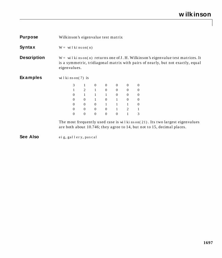
wilkinson
1697
1wilkinsonPurpose Wilkinson’s eigenvalue test matrix
Syntax W = wilkinson(n)
Description W = wilkinson(n) returns one of J. H. Wilkinson’s eigenvalue test matrices. Itis a symmetric, tridiagonal matrix with pairs of nearly, but not exactly, equaleigenvalues.
Examples wilkinson(7) is
3 1 0 0 0 0 01 2 1 0 0 0 00 1 1 1 0 0 00 0 1 0 1 0 00 0 0 1 1 1 00 0 0 0 1 2 10 0 0 0 0 1 3
The most frequently used case is wilkinson(21). Its two largest eigenvaluesare both about 10.746; they agree to 14, but not to 15, decimal places.
See Also eig, gallery, pascal
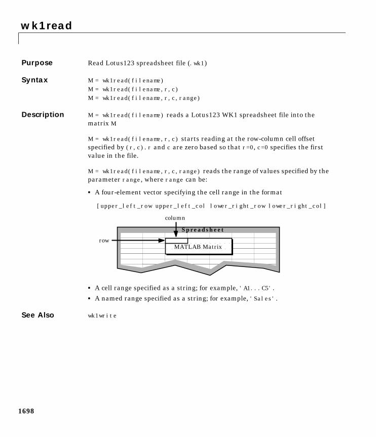
wk1read
1698
1wk1readPurpose Read Lotus123 spreadsheet file (.wk1)
Syntax M = wk1read(filename)M = wk1read(filename,r,c)M = wk1read(filename,r,c,range)
Description M = wk1read(filename) reads a Lotus123 WK1 spreadsheet file into thematrix M.
M = wk1read(filename,r,c) starts reading at the row-column cell offsetspecified by (r,c). r and c are zero based so that r=0, c=0 specifies the firstvalue in the file.
M = wk1read(filename,r,c,range) reads the range of values specified by theparameter range, where range can be:
• A four-element vector specifying the cell range in the format
[upper_left_row upper_left_col lower_right_row lower_right_col]
• A cell range specified as a string; for example, 'A1...C5'.
• A named range specified as a string; for example, 'Sales'.
See Also wk1write
MATLAB Matrix
Spreadsheet
column
row
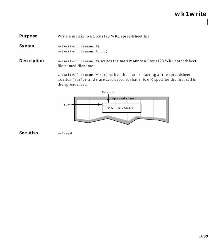
wk1write
1699
1wk1writePurpose Write a matrix to a Lotus123 WK1 spreadsheet file
Syntax wk1write(filename,M)wk1write(filename,M,r,c)
Description wk1write(filename,M) writes the matrix M into a Lotus123 WK1 spreadsheetfile named filename.
wk1write(filename,M,r,c) writes the matrix starting at the spreadsheetlocation (r,c). r and c are zero based so that r=0, c=0 specifies the first cell inthe spreadsheet.
See Also wk1read
MATLAB Matrix
Spreadsheet
column
row
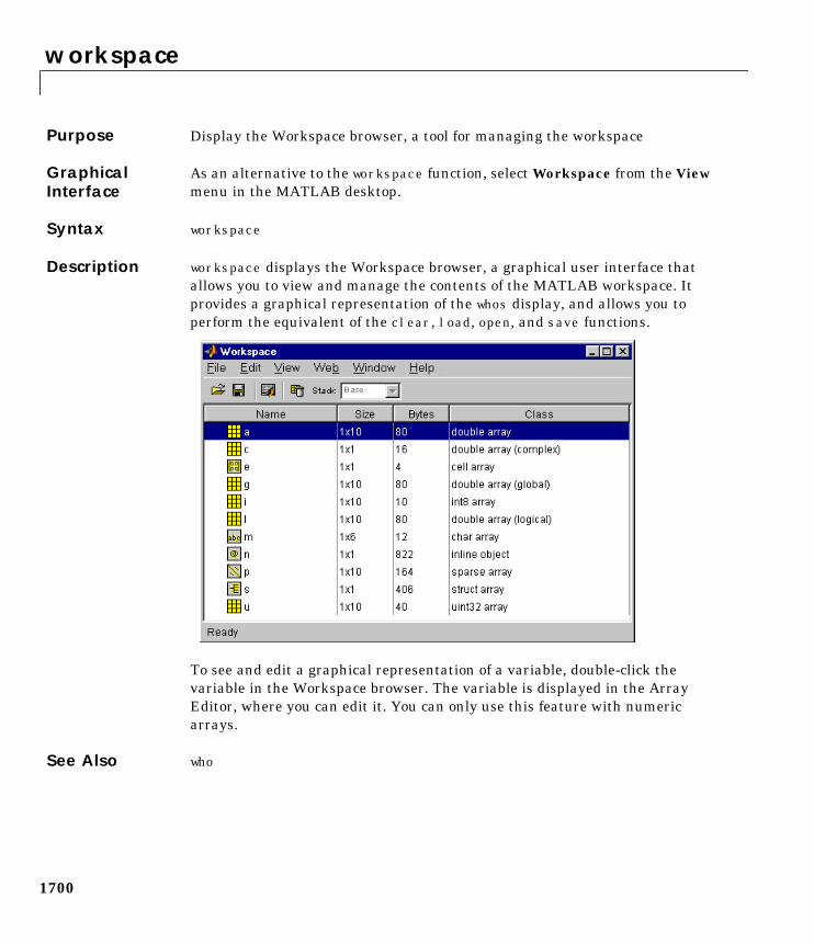
workspace
1700
1workspacePurpose Display the Workspace browser, a tool for managing the workspace
GraphicalInterface
As an alternative to the workspace function, select Workspace from the Viewmenu in the MATLAB desktop.
Syntax workspace
Description workspace displays the Workspace browser, a graphical user interface thatallows you to view and manage the contents of the MATLAB workspace. Itprovides a graphical representation of the whos display, and allows you toperform the equivalent of the clear, load, open, and save functions.
To see and edit a graphical representation of a variable, double-click thevariable in the Workspace browser. The variable is displayed in the ArrayEditor, where you can edit it. You can only use this feature with numericarrays.
See Also who
xlabel, ylabel, zlabel
1701
1xlabel, ylabel, zlabelPurpose Label the x-, y-, and z-axis
Syntax xlabel('string')xlabel(fname)xlabel(...,'PropertyName',PropertyValue,...)h = xlabel(...)
ylabel(...)h = ylabel(...)
zlabel(...)h = zlabel(...)
Description Each axes graphics object can have one label for the x-, y-, and z-axis. The labelappears beneath its respective axis in a two-dimensional plot and to the side orbeneath the axis in a three-dimensional plot.
xlabel('string') labels the x-axis of the current axes.
xlabel(fname) evaluates the function fname, which must return a string, thendisplays the string beside the x-axis.
xlabel(...,'PropertName',PropertyValue,...) specifies property nameand property value pairs for the text graphics object created by xlabel.
h = xlabel(...), h = ylabel(...), and h = zlabel(...) return the handleto the text object used as the label.
ylabel(...) and zlabel(...) label the y-axis and z-axis, respectively, of thecurrent axes.
Remarks Re-issuing an xlabel, ylabel, or zlabel command causes the new label toreplace the old label.
For three-dimensional graphics, MATLAB puts the label in the front or side,so that it is never hidden by the plot.
See Also text, title
xlim, ylim, zlim
1702
1xlim, ylim, zlimPurpose Set or query axis limits
Syntax Note that the syntax for each of these three functions is the same; only the xlimfunction is used for simplicity. Each operates on the respective x-, y-, or z-axis.
xlimxlim([xmin xmax])xlim('mode')xlim('auto')xlim('manual')xlim(axes_handle,...)
Description xlim with no arguments returns the respective limits of the current axes.
xlim([xmin xmax]) sets the axis limits in the current axes to the specifiedvalues.
xlim('mode') returns the current value of the axis limits mode, which can beeither auto (the default) or manual.
xlim('auto') sets the axis limit mode to auto.
xlim('manual') sets the respective axis limit mode to manual.
xlim(axes_handle,...) performs the set or query on the axes identified bythe first argument, axes_handle. When you do not specify an axes handle,these functions operate on the current axes.
Remarks xlim, ylim, and zlim set or query values of the axes object XLim, YLim, ZLim,and XLimMode, YLimMode, ZLimMode properties.
When the axis limit modes are auto (the default), MATLAB uses limits thatspan the range of the data being displayed and are round numbers. Setting avalue for any of the limits also sets the corresponding mode to manual. Notethat high-level plotting functions like plot and surf reset both the modes andthe limits. If you set the limits on an existing graph and want to maintain theselimits while adding more graphs, use the hold command.
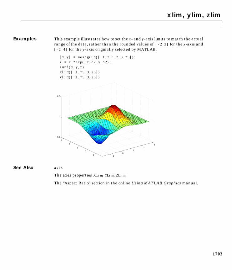
xlim, ylim, zlim
1703
Examples This example illustrates how to set the x- and y-axis limits to match the actualrange of the data, rather than the rounded values of [-2 3] for the x-axis and[-2 4] for the y-axis originally selected by MATLAB.
[x,y] = meshgrid([−1.75:.2:3.25]);z = x.*exp(−x.^2−y.^2);surf(x,y,z)xlim([−1.75 3.25])ylim([−1.75 3.25])
See Also axis
The axes properties XLim, YLim, ZLim
The “Aspect Ratio” section in the online Using MATLAB Graphics manual.
−10
12
3
−1
0
1
2
3
−0.5
0
0.5
xlsfinfo
1704
1xlsfinfoPurpose Determine if file contains Microsoft Excel (.xls) spreadsheet
Syntax [A, Descr] = xlsfinfo('filename')
Description [A, Descr] = xlsfinfo('filename') returns the character array 'MicrosoftExcel Spreadsheet' in A if filename is an Excel spreadsheet. Returns anempty string if filename is not an Excel spreadsheet. Descr is a cell array ofstrings containing the name of each spreadsheet in the file.
Examples When filename is an Excel spreadsheet:
[a,descr] = xlsfinfo('tempdata.xls')
a =
Microsoft Excel Spreadsheet
descr =
'Sheet1'
See Also xlsread
xlsread
1705
1xlsreadPurpose Read Microsoft Excel spreadsheet file (.xls)
Syntax A = xlsread('filename')[A, B ] = xlsread('filename')
[...] = xlsread('filename','sheetname')
Description A = xlsread('filename') returns numeric data in array A from the first sheetin Microsoft Excel spreadsheet file named filename. xlsread ignores leadingrows or columns of text. However, if a cell not in a leading row or column isempty or contains text, xlsread puts a NaN in its place in A.
[A, B]= xlsread('filename') returns numeric data in array A, text data incell array B. If the spreadsheet contains leading rows or columns of text,xlsread returns only those cells in B. If the spreadsheet contains text that isnot in a row or column header, xlsread returns a cell array the same size asthe original spreadsheet with text strings in the cells that correspond to text inthe original spreadsheet. All cells that correspond to numeric data are empty.
[...]= xlsread('filename','sheetname') read sheet specified insheetname. Returns an error if sheetname does not exist. To determine thenames of the sheets in a spreadsheet file, use xlsfinfo.
Handling Excel Date ValuesWhen reading date fields from Excel files, you must convert the Excel datevalues into MATLAB date values. Both Microsoft Excel and MATLABrepresent dates as serial days elapsed from some reference date. However,Microsoft Excel uses January 1, 1900 as the reference date and MATLAB usesJanuary 1, 0000.
For example, if your Excel file contains these date values,
4/12/004/13/004/14/00
use this code to convert the dates to MATLAB dates.
excelDates = xlsread('filename')matlabDates = datenum('30-Dec-1899') + excelDatesdatestr(matlabDates,2)ans =
xlsread
1706
04/12/0004/13/0004/14/00
Examples Example 1 – Reading Numeric DataThe Microsoft Excel spreadsheet file, testdata1.xls, contains this data:
1 62 73 84 95 10
To read this data into MATLAB, use this command:
A = xlsread('testdata1.xls')A =
1 62 73 84 95 10
Example 2 – Handling Text DataThe Microsoft Excel spreadsheet file, testdata2.xls, contains a mix ofnumeric and text data.
1 62 73 84 95 text
xlsread
1707
xlsread puts a NaN in place of the text data in the result.
A = xlsread('testdata2.xls')A =
1 62 73 84 95 NaN
Example 3 – Handling Files with Row or Column HeadersThe Microsoft Excel spreadsheet file, tempdata.xls, contains two columns ofnumeric data with text headers for each column:
Time Temp12 9813 9914 97
If you want to import only the numeric data, use xlsread with a single returnargument. xlsread ignores a leading row or column of text in the numericresult.
ndata = xlsread('tempdata.xls')
ndata =
12 98 13 99 14 97
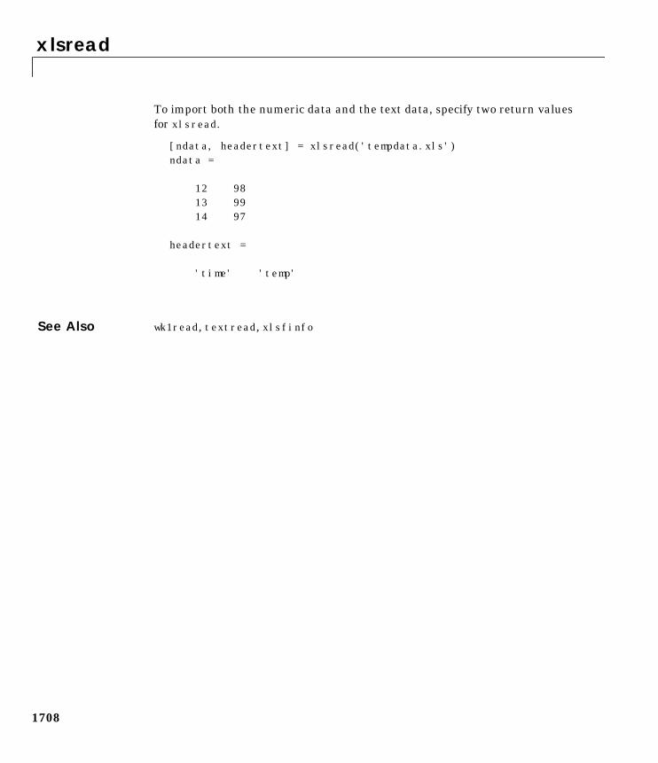
xlsread
1708
To import both the numeric data and the text data, specify two return valuesfor xlsread.
[ndata, headertext] = xlsread('tempdata.xls')ndata =
12 98 13 99 14 97
headertext =
'time' 'temp'
See Also wk1read, textread, xlsfinfo
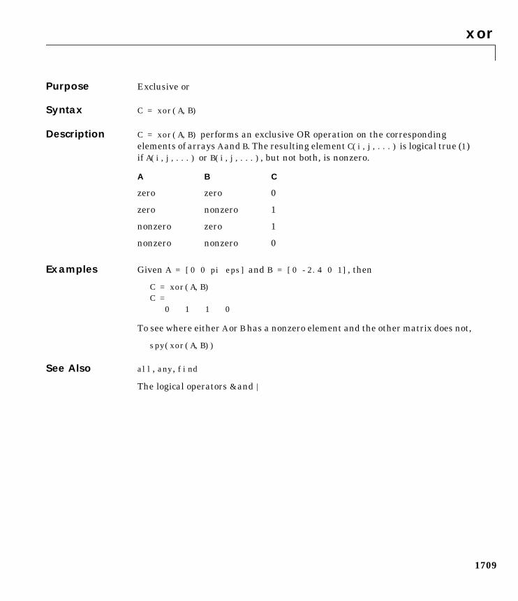
xor
1709
1xorPurpose Exclusive or
Syntax C = xor(A,B)
Description C = xor(A,B) performs an exclusive OR operation on the correspondingelements of arrays A and B. The resulting element C(i,j,...) is logical true (1)if A(i,j,...) or B(i,j,...), but not both, is nonzero.
Examples Given A = [0 0 pi eps] and B = [0 -2.4 0 1], then
C = xor(A,B)C = 0 1 1 0
To see where either A or B has a nonzero element and the other matrix does not,
spy(xor(A,B))
See Also all, any, find
The logical operators & and |
A B C
zero zero 0
zero nonzero 1
nonzero zero 1
nonzero nonzero 0
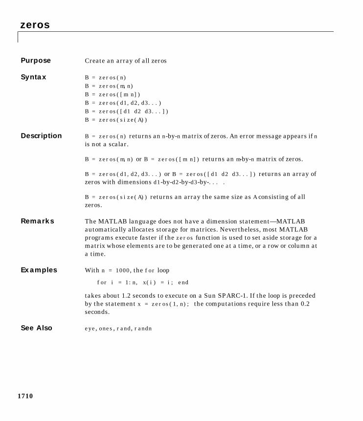
zeros
1710
1zerosPurpose Create an array of all zeros
Syntax B = zeros(n)B = zeros(m,n)B = zeros([m n])B = zeros(d1,d2,d3...)B = zeros([d1 d2 d3...])B = zeros(size(A))
Description B = zeros(n) returns an n-by-n matrix of zeros. An error message appears if nis not a scalar.
B = zeros(m,n) or B = zeros([m n]) returns an m-by-n matrix of zeros.
B = zeros(d1,d2,d3...) or B = zeros([d1 d2 d3...]) returns an array ofzeros with dimensions d1-by-d2-by-d3-by-... .
B = zeros(size(A)) returns an array the same size as A consisting of allzeros.
Remarks The MATLAB language does not have a dimension statement—MATLABautomatically allocates storage for matrices. Nevertheless, most MATLABprograms execute faster if the zeros function is used to set aside storage for amatrix whose elements are to be generated one at a time, or a row or column ata time.
Examples With n = 1000, the for loop
for i = 1:n, x(i) = i; end
takes about 1.2 seconds to execute on a Sun SPARC-1. If the loop is precededby the statement x = zeros(1,n); the computations require less than 0.2seconds.
See Also eye, ones, rand, randn
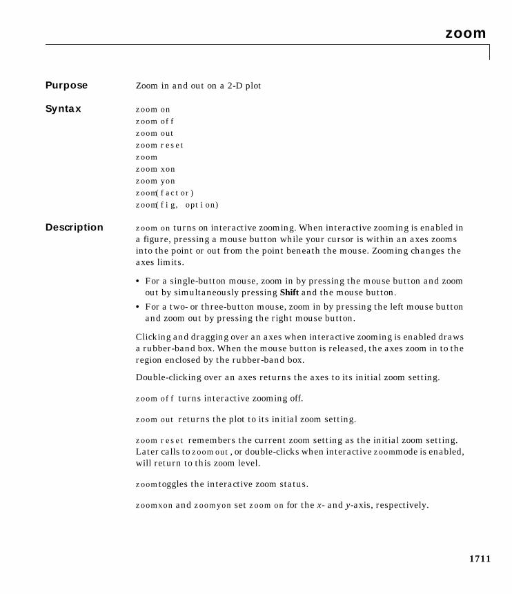
zoom
1711
1zoomPurpose Zoom in and out on a 2-D plot
Syntax zoom onzoom offzoom outzoom resetzoomzoom xonzoom yonzoom(factor)zoom(fig, option)
Description zoom on turns on interactive zooming. When interactive zooming is enabled ina figure, pressing a mouse button while your cursor is within an axes zoomsinto the point or out from the point beneath the mouse. Zooming changes theaxes limits.
• For a single-button mouse, zoom in by pressing the mouse button and zoomout by simultaneously pressing Shift and the mouse button.
• For a two- or three-button mouse, zoom in by pressing the left mouse buttonand zoom out by pressing the right mouse button.
Clicking and dragging over an axes when interactive zooming is enabled drawsa rubber-band box. When the mouse button is released, the axes zoom in to theregion enclosed by the rubber-band box.
Double-clicking over an axes returns the axes to its initial zoom setting.
zoom off turns interactive zooming off.
zoom out returns the plot to its initial zoom setting.
zoom reset remembers the current zoom setting as the initial zoom setting.Later calls to zoom out, or double-clicks when interactive zoommode is enabled,will return to this zoom level.
zoom toggles the interactive zoom status.
zoom xon and zoom yon set zoom on for the x- and y-axis, respectively.
zoom
1712
zoom(factor) zooms in or out by the specified zoom factor, without affectingthe interactive zoom mode. Values greater than 1 zoom in by that amount,while numbers greater than 0 and less than 1 zoom out by 1/factor.
zoom(fig, option) Any of the above options can be specified on a figure otherthan the current figure using this syntax.
Remarks zoom changes the axes limits by a factor of two (in or out) each time you pressthe mouse button while the cursor is within an axes. You can also click anddrag the mouse to define a zoom area, or double-click to return to the initialzoom level.
I-1
Index
Symbols 1690! 1388% 1388' 1388( ) 1388, 1388. 1388... 1388../ref/axes_prope.html#ALim 1508< 1280= 1388== 1280> 1280 1388~= 1280 1280 1280
Numericsπ (pi) 1145, 1243, 13601-norm 1247
AAccelerator
Uimenu property 1632all 1536allocation of storage (automatic) 1710AlphaData
surface property 1508AlphaDataMapping
patch property 1092surface property 1508
AmbientStrength
Patch property 1092
Surface property 1509annotating plots 1159arguments, M-file
passing variable numbers of 1653array
product of elements 1200of random numbers 1236, 1238removing first n singleton dimensions of 1355removing singleton dimensions of 1418reshaping 1285shifting dimensions of 1355size of 1363sorting elements of 1373structure 1294, 1349sum of elements 1491swapping dimensions of 1143of all zeros 1710
arraysediting 1700
ASCII dataconverting sparse matrix after loading from
1382saving to disk 1318
aspect ratio of axes 1114axes
setting and querying limits 1702setting and querying plot box aspect ratio
1114axes
editing 1159azimuth (spherical coordinates) 1393azimuth of viewpoint 1660
BBackFaceLighting
Index
I-2
Surface property 1509BackFaceLightingpatch property 1093BackGroundColor
Uicontrol property 1611badly conditioned 1247binary data
saving to disk 1318bold font
TeX characters 1569braces, curly (special characters) 1388brackets (special characters) 1388Buckminster Fuller 1542BusyAction
patch property 1093rectangle property 1263Root property 1299Surface property 1509Text property 1560Uicontextmenu property 1598Uicontrol property 1611Uimenu property 1633
ButtonDownFcn
patch property 1093rectangle property 1263Root property 1299Surface property 1510Text property 1560Uicontextmenu property 1598Uicontrol property 1612Uimenu property 1633
Ccaching
MATLAB directory 1110CallBack
Uicontextmenu property 1598
Uicontrol property 1612Uimenu property 1633
CallbackObject, Root property 1299CaptureMatrix, Root property 1299CaptureRect, Root property 1299Cartesian coordinates 1166, 1393case
in switch statement (defined) 1531lower to upper 1651
Cayley-Hamilton theorem 1181CData
Surface property 1510Uicontrol property 1613
CDataMapping
patch property 1095Surface property 1510
CDatapatch property 1093characters
conversion, in format specification string 1409escape, in format specification string 1410
check boxes 1603Checked, Uimenu property 1634checkerboard pattern (example) 1283Children
patch property 1096rectangle property 1263Root property 1299Surface property 1511Text property 1560Uicontextmenu property 1598Uicontrol property 1613Uimenu property 1634
Cholesky factorizationlower triangular factor 1079minimum degree ordering and (sparse) 1540
Clipping
rectangle property 1263
Index
I-3
Root property 1299Surface property 1511Text property 1561Uicontextmenu property 1599Uicontrol property 1613Uimenu property 1634
Clippingpatch property 1096closest triangle search 1593closing
MATLAB 1229Color
Text property 1561colormaps
converting from RGB to HSV 1289plotting RGB components 1290
comma (special characters) 1390complex
numbers, sorting 1373, 1374unitary matrix 1213
complex Schur form 1331condition number of matrix 1247context menu 1595continuation (..., special characters) 1389continued fraction expansion 1242conversion
cylindrical to Cartesian 1166full to sparse 1379lowercase to uppercase 1651partial fraction expansion to pole-residue
1286polar to Cartesian 1166pole-residue to partial fraction expansion
1286real to complex Schur form 1316spherical to Cartesian 1393string to numeric array 1435
conversion characters in format specificationstring 1409
coordinate system and viewpoint 1660coordinates
Cartesian 1166, 1393cylindrical 1166polar 1166spherical 1393
CreateFcn
patch property 1096rectangle property 1264Root property 1299Surface property 1511Text property 1561Uicontextmenu property 1599Uicontrol property 1613Uimenu property 1634
cubic interpolation 1123curly braces (special characters) 1388current directory 1208CurrentFigure, Root property 1299Curvature, rectangle property 1264curve fitting (polynomial) 1174Cuthill-McKee ordering, reverse 1540, 1542cylindrical coordinates 1166
Ddata
ASCII, saving to disk 1318binary, dependence upon array size and type
1319binary, saving to disk 1318computing 2-D stream lines 1440computing 3-D stream lines 1442formatting 1408reading from files 1572
Index
I-4
reducing number of elements in 1275smoothing 3-D 1372writing to strings 1408
data, ASCIIconverting sparse matrix after loading from
1382debugging
M-files 1201decimal point (.)
(special characters) 1389decomposition
“economy-size” 1213, 1527orthogonal-triangular (QR) 1213Schur 1331singular value 1241, 1527
definite integral 1222DeleteFcn
Root property 1300Surface property 1511Text property 1561Uicontextmenu property 1599Uicontrol property 1613Uimenu property 1634
DeleteFcn, rectangle property 1264DeleteFcnpatch property 1096dependence, linear 1487derivative
polynomial 1172detecting
positive, negative, and zero array elements1359
diagonalk-th (illustration) 1587sparse 1384
dialog boxprint 1199question 1227
warning 1675Diary, Root property 1300DiaryFile, Root property 1300differences
between sets 1348differential equation solvers
ODE boundary value problemsextracting properties of 1585, 1586
parabolic-elliptic PDE problems 1129DiffuseStrength
Surface property 1512DiffuseStrengthpatch property 1097dimension statement (lack of in MATLAB ) 1710dimensions
size of 1363direct term of a partial fraction expansion 1286directories
listing MATLAB files in 1687MATLAB
caching 1110removing from search path 1295
directorytemporary system 1547
directory, current 1208discontinuities, eliminating (in arrays of phase
angles) 1650division
remainder after 1282
EEcho, Root property 1300EdgeAlpha
patch property 1097surface property 1512
EdgeColor
patch property 1097
Index
I-5
Surface property 1512EdgeColor, rectangle property 1265EdgeLighting
patch property 1098Surface property 1513
editable text 1603eigenvalue
modern approach to computation of 1170problem 1173problem, generalized 1173problem, polynomial 1173Wilkinson test matrix and 1697
eigenvectormatrix, generalized 1235
elevation (spherical coordinates) 1393elevation of viewpoint 1660Enable
Uicontrol property 1614Uimenu property 1635
end of line, indicating 1390equal sign (special characters) 1389EraseMode
rectangle property 1265Surface property 1513Text property 1562
EraseModepatch property 1098error messages
Out of memory 1073ErrorMessage, Root property 1300ErrorType, Root property 1301escape characters in format specification string
1410examples
reducing number of patch faces 1272reducing volume data 1275subsampling volume data 1489
Excel spreadsheets
loading 1705exclamation point (special characters) 1390executing statements repeatedly 1693execution
improving speed of by setting aside storage1710
pausing M-file 1113time for M-files 1201
extension, filename.mat 1318
Extent
Text property 1563Uicontrol property 1615
FFaceAlphapatch property 1099FaceAlphasurface property 1514FaceColor
Surface property 1515FaceColor, rectangle property 1266FaceColorpatch property 1100FaceLighting
Surface property 1515FaceLightingpatch property 1100faces, reducing number in patches 1271Faces,patch property 1100FaceVertexAlphaData, patch property 1101FaceVertexCData,patch property 1102factorization
QZ 1173, 1235See also decomposition
factorization, Choleskyminimum degree ordering and (sparse) 1540
featuresundocumented 1689
Figure
Index
I-6
redrawing 1278figures
annotating 1159saving 1323
filenametemporary 1548
filename extension.mat 1318
filescontents, listing 1594Excel spreadsheets
loading 1705fig 1323figure, saving 1323listing
in directory 1687listing contents of 1594locating 1690mdl 1323model, saving 1323opening
in Web browser 1684pathname for 1690reading
data from 1572README 1689sound
reading 1681writing 1683
.wav
reading 1681writing 1683
WK1loading 1698writing to 1699
findingsign of array elements 1359
finish.m 1229fixed-width font
text 1563uicontrols 1615
FixedWidthFontName, Root property 1300floating-point arithmetic, IEEE
smallest postive number 1252flow control
return 1288switch 1531while 1693
fontfixed-width, text 1563fixed-width, uicontrols 1615
FontAngle
Text property 1563Uicontrol property 1615
FontName
Text property 1563Uicontrol property 1615
fontsbold 1564italic 1563specifying size 1564TeX characters
bold 1569italics 1569specifying family 1569specifying size 1569
units 1564FontSize
Text property 1564Uicontrol property 1616
FontUnits
Text property 1564Uicontrol property 1616
FontWeight
Index
I-7
Text property 1564Uicontrol property 1616
ForegroundColor
Uicontrol property 1616Uimenu property 1635
Format 1301format
specification string, matching file data to 1420FormatSpacing, Root property 1301formatting data 1408fraction, continued 1242fragmented memory 1073frames 1604functions
locating 1690pathname for 1690that work down the first non-singleton
dimension 1355
GGaussian elimination
Gauss Jordan elimination with partial pivoting1314
generalized eigenvalue problem 1173geodesic dome 1542Givens rotations 1217, 1218graphics objects
Patch 1080resetting properties 1284Root 1296setting properties 1342Surface 1500Text 1553uicontextmenu 1595Uicontrol 1603Uimenu 1628
graphsediting 1159
Greek letters and mathematical symbols 1568griddata3 1670GUIs, printing 1195
HHadamard matrix
subspaces of 1487HandleVisibility
patch property 1103rectangle property 1266Root property 1301Surface property 1516Text property 1564Uicontextmenu property 1599Uicontrol property 1616Uimenu property 1635
helpPlot Editor 1160
HitTest
Patch property 1104rectangle property 1267Root property 1301Surface property 1516Text property 1565Uicontextmenu property 1600Uicontrol property 1617
HorizontalAlignment
Text property 1566Uicontrol property 1617
horzcat (M-file function equivalent for [,]) 1390hyperbolic
secant 1334sine 1360tangent 1545
Index
I-8
hyperplanes, angle between 1487
Iidentity matrix
sparse 1391IEEE floating-point arithmetic
smallest positive number 1252indices, array
of sorted elements 1373integration
quadrature 1222interpolated shading and printing 1195Interpreter, Text property 1566Interruptible
patch property 1104rectangle property 1267Root property 1301Surface property 1517Text property 1566Uicontextmenu property 1600Uicontrol property 1618Uimenu property 1636
involutary matrix 1079italics font
TeX characters 1569
JJacobi rotations 1407Java version used by MATLAB 1658
Kkeyboard mode
terminating 1288
LLabel, Uimenu property 1637labeling
axes 1701LaTeX, see TeX 1567least squares
polynomial curve fitting 1174problem, overdetermined 1150
limits of axes, setting and querying 1702Line
properties 1263line
editing 1159linear dependence (of data) 1487linear equation systems
solving overdetermined 1215–1216lines
computing 2-D stream 1440computing 3-D stream 1442drawing stream lines 1444
LineStyle
patch property 1105rectangle property 1267Surface object 1517
LineWidth
Patch property 1105rectangle property 1268Surface property 1517
list boxes 1604defining items 1622
ListboxTop, Uicontrol property 1619logical operations
XOR 1709Lotus WK1 files
loading 1698writing 1699
lower triangular matrix 1587
Index
I-9
lowercase to uppercase 1651
Mmachine epsilon 1693Marker
Patch property 1105Surface property 1517
MarkerEdgeColor
Patch property 1106Surface property 1518
MarkerFaceColor
Patch property 1106Surface property 1519
MarkerSize
Patch property 1106Surface property 1519
MAT-file 1318converting sparse matrix after loading from
1382MAT-files
listing for directory 1687MATLAB
quitting 1229version number, displaying 1656
MATLAB startup file 1424matlab.mat 1318matrix
complex unitary 1213condition number of 1247converting to from string 1419decomposition 1213Hadamard 1487Hermitian Toeplitz 1581involutary 1079lower triangular 1587magic squares 1491
orthonormal 1213Pascal 1079, 1180permutation 1213pseudoinverse 1150reduced row echelon form of 1314replicating 1283rotating 90˚ 1309Schur form of 1316, 1331sorting rows of 1374sparse See sparse matrixsquare root of 1415subspaces of 1487Toeplitz 1581trace of 1582transposing 1389unitary 1527upper triangular 1590Vandermonde 1176Wilkinson 1385, 1697writing to spreadsheet 1699
Max, Uicontrol property 1619memory
minimizing use of 1073variables in 1695
MeshStyle, Surface property 1519message
error See error messagewarning See warning message
MEX-fileslisting for directory 1687
M-filepausing execution of 1113
M-filescreating
in MATLAB directory 1110debugging with profile 1201listing names of in a directory 1687
Index
I-10
optimizing 1201Microsoft Excel files
loading 1705Min, Uicontrol property 1619minimum degree ordering 1540models
saving 1323Moore-Penrose pseudoinverse 1150multidimensional arrays
rearranging dimensions of 1143removing singleton dimensions of 1418reshaping 1285size of 1363sorting elements of 1373
NNaN (Not-a-Number)
returned by rem 1282nonzero entries
number of in sparse matrix 1379nonzero entries (in sparse matrix)
replacing with ones 1401norm
1-norm 1247pseudoinverse and 1150–??
NormalMode
Patch property 1106Surface property 1519
numbersprime 1184random 1236, 1238real 1250smallest positive 1252
Ooperating system command, issuing 1390operators
relational 1280special characters 1388
optimizing M-file execution 1201ordering
minimum degree 1540reverse Cuthill-McKee 1540, 1542
orthogonal-triangular decomposition 1213orthonormal matrix 1213Out of memory (error message) 1073overdetermined equation systems, solving 1215–
1216
Ppack 1073pagedlg 1075pagesetupdlg 1076Parent
Patch property 1107rectangle property 1268Root property 1302Surface property 1519Text property 1567Uicontextmenu property 1601Uicontrol property 1620Uimenu property 1637
parentheses (special characters) 1389pareto 1077partial fraction expansion 1286partialpath 1078Pascal matrix 1079, 1180Patch
converting a surface to 1498creating 1080
Index
I-11
defining default properties 1086properties 1092reducing number of faces 1271reducing size of face 1356
patch 1080path
current 1110removing directories from 1295viewing 1112
path 1110pathname
partial 1078pathnames
of functions or files 1690relative 1078
pathtool 1112pause 1113pausing M-file execution 1113pbaspect 1114pcg 1119pchip 1123pcode 1125pcolor 1126PDE See Partial Differential Equationspdepe 1129pdeval 1140percent sign (special characters) 1390period (special characters) 1389perms 1142permutation
of array dimensions 1143matrix 1213random 1240
permutations of n elements 1142permute 1143persistent 1144persistent variable 1144
phase, complexcorrecting angles 1650
pi 1145pi (π) 1145, 1243, 1360pie 1146pie3 1148pinv 1150plot 1152
editing 1159plot box aspect ratio of axes 1114Plot Editor
help for 1160interface 1160, 1207
plot, volumetricslice plot 1366
plot3 1157plotedit 1159plotmatrix 1162plotting
2-D plot 11523-D plot 1157plot with two y-axes 1164ribbon plot 1291rose plot 1307scatter plot 1162, 1327scatter plot, 3-D 1329semilogarithmic plot 1337stairstep plot 1422stem plot 1427stem plot, 3-D 1429surface plot 1494volumetric slice plot 1366
plotting See visualizingplotyy 1164PointerLocation, Root property 1302PointerWindow, Root property 1302pol2cart 1166
Index
I-12
polar 1167polar coordinates 1166poles of transfer function 1286poly 1169polyarea 1171polyder 1172polyeig 1173polyfit 1174polygon
area of 1171creating with patch 1080
polyint 1177polynomial
analytic integration 1177characteristic 1169–1170, 1305coefficients (transfer function) 1286curve fitting with 1174derivative of 1172eigenvalue problem 1173evaluation 1178evaluation (matrix sense) 1180
polyval 1178polyvalm 1180pop-up menus 1604
defining choices 1622Position
Text property 1567Uicontextmenu property 1601Uicontrol property 1620Uimenu property 1637
Position, rectangle property 1268PostScript
printing interpolated shading 1195pow2 1182ppval 1183prime numbers 1184primes 1184
print 1185printdlg 1199printer drivers
GhostScript drivers 1186interploated shading 1195MATLAB printer drivers 1186
printingGUIs 1195interpolated shading 1195on MS-Windows 1193with a variable filename 1197with non-normal EraseMode 1099, 1265, 1514,
1562printing tips 1193printing, suppressing 1390printopt 1185prod 1200product
of array elements 1200profile 1201profile report 1204profreport 1204propedit 1206Property Editor
interface 1207pseudoinverse 1150push buttons 1604pwd 1208
Qqmr 1209qr 1213QR decomposition 1213
deleting a column from 1217inserting a column into 1218
qrdelete 1217
Index
I-13
qrinsert 1218quad 1222quad8 1222quadl 1225quadrature 1222questdlg 1227quit 1229quitting MATLAB 1229quiver 1231quiver3 1233qz 1235QZ factorization 1173, 1235
Rradio buttons 1604rand 1236, 1492randn 1238random
numbers 1236, 1238permutation 1240sparse matrix 1405, 1406symmetric sparse matrix 1407
randperm 1240rank 1241rank of a matrix 1241rat 1242rational fraction approximation 1242rats 1242rbbox 1245, 1278rcond 1247readasync 1248reading
data from files 1572formatted data from strings 1419
README file 1689real 1250
real numbers 1250realmax 1251realmin 1252rearranging arrays
removing first n singleton dimensions 1355removing singleton dimensions 1418reshaping 1285shifting dimensions 1355swapping dimensions 1143
rearranging matricesrotating 90˚ 1309transposing 1389
record 1253rectint 1270RecursionLimit
Root property 1302reduced row echelon form 1314reducepatch 1271reducevolume 1275refresh 1278rehash 1279relational operators 1280rem 1282remainder after division 1282repeatedly executing statements 1693replicating a matrix 1283repmat 1283reports
profile 1204reset 1284reshape 1285residue 1286residues of transfer function 1286return 1288reverse Cuthill-McKee ordering 1540, 1542RGB, converting to HSV 1289rgb2hsv 1289
Index
I-14
rgbplot 1290ribbon 1291right-click and context menus 1595rmfield 1294rmpath 1295root 1296Root graphics object 1296root object 1296root, see rootobject 1296roots 1295roots of a polynomial 1169–1170, 1305rose 1304, 1307rot90 1309rotate 1310rotate3d 1312Rotation, Text property 1567rotations
Givens 1217, 1218Jacobi 1407
roundto nearest integer 1313
round 1313roundoff error
characteristic polynomial and 1170partial fraction expansion and 1287polynomial roots and 1305sparse matrix conversion and 1383
rref 1314rrefmovie 1314rsf2csf 1316rubberband box 1245
Ssave 1318save
serial port I/O 1321
saveas 1323saving
ASCII data 1318workspace variables 1318
scatter 1327scatter3 1329schur 1331Schur decomposition 1331Schur form of matrix 1316, 1331ScreenDepth, Root property 1302ScreenSize, Root property 1303script 1333search path 1295
MATLAB’s 1110modifying 1112viewing 1112
sec 1334secant 1334sech 1334Selected
Patch property 1107rectangle property 1268Root property 1303Surface property 1519Text property 1567Uicontextmenu property 1601Uicontrol property 1620Uimenu property 1637
selecting areas 1245SelectionHighlight
Patch property 1107rectangle property 1268Surface property 1520Text property 1567Uicontextmenu property 1601Uicontrol property 1621
selectmoveresize 1336
Index
I-15
semicolon (special characters) 1390semilogx 1337semilogy 1337Separator, Uimenu property 1637serial 1339serialbreak 1341set 1342set
serial port I/O 1345set operations
difference 1348exclusive or 1351union 1647unique 1648
setdiff 1348setfield 1349setstr 1350setxor 1351shading 1352shading colors in surface plots 1352shiftdim 1355ShowHiddenHandles, Root property 1303shrinkfaces 1356shutdown 1229sign 1359signum function 1359Simpson’s rule, adaptive recursive 1223Simulink
version number, displaying 1656sin 1360sine 1360single quote (special characters) 1389singular value
decomposition 1241, 1527rank and 1241
sinh 1360size 1363
size
serial port I/O 1365size of array dimensions 1363size of fonts, see also FontSize property 1569size vector 1285, 1363slice 1366sliders 1605SliderStep, Uicontrol property 1621smooth3 1372smoothing 3-D data 1372soccer ball (example) 1542sort 1373sorting
array elements 1373matrix rows 1374
sortrows 1374sound
converting vector into 1375, 1377files
reading 1681writing 1683
playing 1679recording 1682resampling 1679sampling 1682
sound 1375, 1377soundcap 1376source control systems
undo checkout 1646spalloc 1378sparse 1379sparse matrices
solving least squares linear systems 1214sparse matrix
allocating space for 1378applying function only to nonzero elements of
1392
Index
I-16
diagonal 1384identity 1391number of nonzero elements in 1379random 1405, 1406random symmetric 1407replacing nonzero elements of with ones 1401results of mixed operations on 1380visualizing sparsity pattern of 1413
spaugment 1381spconvert 1382spdiags 1384SpecularColorReflectance
Patch property 1107Surface property 1520
SpecularExponent
Patch property 1107Surface property 1520
SpecularStrength
Patch property 1107Surface property 1520
speye 1391spfun 1392sph2cart 1393sphere 1394spherical coordinates 1393spinmap 1396spline 1397spones 1401spparms 1402sprand 1405sprandn 1406sprandsym 1407spreadsheets
loading WK1 files 1698loading XLS files 1705writing from matrix 1699
sqrt 1414
sqrtm 1415square root
of a matrix 1415of array elements 1414
squeeze 1418sscanf 1419stairs 1422standard deviation 1425startup 1424startup file 1424static text 1605std 1425stem 1427stem3 1429stopasync 1431stopwatch timer 1578storage
sparse 1379str2num 1434, 1435strcat 1436strcmp 1437strcmpi 1439stream lines
computing 2-D 1440computing 3-D 1442drawing 1444
stream2 1440stream3 1442String
Text property 1567Uicontrol property 1621
stringcomparing one to another 1437comparing the first n characters of two 1468converting to numeric array 1435converting to uppercase 1651dictionary sort of 1374
Index
I-17
finding first token in 1475searching and replacing 1474
stringsconverting to matrix (formatted) 1419writing data to 1408
strings 1465strjust 1466strmatch 1467strncmp 1468strncmpi 1469strrep 1474strtok 1475struct2cell 1478structure array
remove field from 1294setting contents of a field of 1349
strvcat 1479Style
Uicontrol property 1622sub2ind 1480subplot 1482subsasgn 1485subscripts
in axis title 1579in text strings 1570
subspace 1487subsref 1488subsref (M-file function equivalent for
A(i,j,k...)) 1390subvolume 1489sum
of array elements 1491sum 1491superiorto 1492superscripts
in axis title 1580in text strings 1570
support 1493surf 1494surf2patch 1498Surface
converting to a patch 1498creating 1500defining default properties 1259, 1503properties 1508
surface 1500surfc 1494surfl 1522surfnorm 1525svd 1527svds 1529switch 1531symamd 1533symbfact 1535symbols in text 1568symmmd 1540symrcm 1542system directory, temporary 1547
TTag
Patch property 1108rectangle property 1268Root property 1303Surface property 1520Text property 1570Uicontextmenu property 1601Uicontrol property 1622Uimenu property 1638
tan 1545tangent 1545
hyperbolic 1545tanh 1545
Index
I-18
tempdir 1547tempname 1548temporary
files 1548system directory 1547
terminal 1549terminating MATLAB 1229TeX commands in text 1567Text
creating 1553defining default properties 1556fixed-width font 1563properties 1560
textsubscripts 1570superscripts 1570
text 1553editing 1159
textread 1572textwrap 1577tic 1578tiling (copies of a matrix) 1283time
elapsed (stopwatch timer) 1578title
with superscript 1579, 1580title 1579toc 1578toeplitz 1581Toeplitz matrix 1581toggle buttons 1605token See also string 1475TooltipString
Uicontrol property 1622trace 1582trace of a matrix 1582transformation
left and right (QZ) 1235trapz 1583treelayout 1585treeplot 1586tril 1587trimesh 1588trisurf 1589triu 1590try 1591tsearch 1592tsearchn 1593Type
Patch property 1108rectangle property 1268Root property 1303Surface property 1520Text property 1570Uicontextmenu property 1601Uicontrol property 1622Uimenu property 1638
type 1594
UUIContextMenu
Patch property 1108rectangle property 1269Surface property 1521Text property 1571
UiContextMenu
Uicontrol property 1623Uicontextmenu
properties 1598Uicontextmenu
Uicontextmenu property 1601uicontextmenu 1595Uicontrol
Index
I-19
defining default properties 1611fixed-width font 1615properties 1611types of 1603
uicontrol 1603uigetfile 1625uiimport 1627Uimenu
creating 1628defining default properties 1632properties 1632
uimenu 1628uint* 1639uint8 1639uiputfile 1640uiresume 1642uisetcolor 1643uisetfont 1644uiwait 1642undocheckout 1646undocumented functionality 1689union 1647unique 1648unitary matrix (complex) 1213Units
Root property 1304Text property 1570Uicontrol property 1623
unwrap 1650upper triangular matrix 1590url
opening in Web browser 1684UserData
Patch property 1108rectangle property 1269Root property 1304Surface property 1521
Text property 1570Uicontextmenu property 1601Uicontrol property 1623Uimenu property 1638
VValue, Uicontrol property 1623Vandermonde matrix 1176var 1652varargout 1653variable numbers of M-file arguments 1653variables
graphical representation of 1700in workspace 1700listing 1695persistent 1144saving 1318sizes of 1695
vectorize 1655ver 1656version 1658version numbers
displaying 1656returned as strings 1658
vertcat (M-file function equivalent for [;]) 1390VertexNormals
Patch property 1108Surface property 1521
VerticalAlignment, Text property 1571Vertices, Patch property 1109view
azimuth of viewpoint 1660coordinate system defining 1660elevation of viewpoint 1660
view 1659viewmtx 1662
Index
I-20
Visible
Patch property 1109rectangle property 1269Root property 1304Surface property 1521Text property 1571Uicontextmenu property 1602Uicontrol property 1624Uimenu property 1638
visualizingsparse matrices 1413
volumescomputing 2-D stream lines 1440computing 3-D stream lines 1442drawing stream lines 1444reducing face size in isosurfaces 1356reducing number of elements in 1275
voronoi 1668
Wwaitbar 1672waitfor 1673waitforbuttonpress 1674warndlg 1675warning message (enabling, suppressing, and
displaying) 1676waterfall 1677.wav files
reading 1681writing 1683
waveplay 1679waverecord 1682wavplay 1679wavread 1681wavrecord 1682wavwrite 1683
web 1684Web browser
pointing to file or url 1684weekday 1686well conditioned 1247what 1687whatsnew 1689which 1690while 1693white space characters, ASCII 1475whitebg 1694who 1695whos 1695wilkinson 1697Wilkinson matrix 1385, 1697WK1 files
loading 1698writing from matrix 1699
wk1read 1698wk1write 1699workspace
consolidating memory 1073predefining variables 1424saving 1318variables in 1695viewing contents of 1700
workspace 1700
Xx-axis limits, setting and querying 1702XData
Patch property 1109Surface property 1521
xlabel 1701xlim 1702XLS files
Index
I-21
loading 1705xlsfinfo 1704xlsread 1705logical XOR 1709xor 1709XOR, printing 1099, 1265, 1514, 1562xyz coordinates See Cartesian coordinates
Yy-axis limits, setting and querying 1702YData
Patch property 1109Surface property 1521
ylabel 1701ylim 1702
Zz-axis limits, setting and querying 1702ZData
Patch property 1109Surface property 1521
zeros 1710zlabel 1701zlim 1702zoom 1711

Index
I-22

Index
I-23

Index
I-24

Index
I-25

Index
I-26

Index
I-27

Index
I-28

Index
I-29

Index
I-30

Index
I-31

Index
I-32

Index
I-33

Index
I-34

Index
I-35

Index
I-36

Index
I-37

Index
I-38