The Joys of Industrial Diversification

in the Stock and Eurobond Markets

Simone Varotto1

ICMA Centre

University of Reading, UK

Abstract

Although the positive effect of international diversification on portfolio risk is well

understood what causes it is still an open issue. Several studies find that the difference in

industrial structure across countries explains little of the total risk reduction achievable in

international portfolios. In this paper we re-appraise the extend of industry effects in the

return volatility of stock portfolios and find them to be substantially larger than it was

previously thought. We also find that both geographical and industrial diversification

cause a significant reduction in the spread return volatility of bond portfolios while their

impact on interest rate risk is much weaker. Maturity, seniority and rating diversification

effects are also investigated.

JEL Classification: G11, G15.

Keywords: International Diversification, Bonds, Stocks, Maturity, Seniority, Credit

Rating.

1 ICMA Centre, University of Reading, Whiteknights Park, Reading RG6 6BA, Tel: +44 (0)118 378 6655, Fax +44 (0)118 9314741, Email: s.varotto@icmacentre.rdg.ac.uk.

1

1. Introduction

Several studies have tried to explain why international diversification is effective in

reducing portfolio risk. Lessard (1974) argues that the systematic risk component of stock

returns in a country is generally not systematic globally. Hence, to a degree, locally

systematic risk can be diversified by distributing portfolio holdings across countries.

Lessard points out that the resulting decline in international portfolio risk depends on

idiosyncrasies between two distinct sources of return variation namely, country risk

factors and industry risk factors. International differences in legal system, monetary and

fiscal policy, access to credit and capital markets justify the existence of country specific

factors. In addition, industrial structures are non-homogeneous across countries. This too

may be responsible for the low covariation of international stock returns. Lessard finds

that industry factors explain a small portion of national stock index returns while much

stronger is the explanatory power of country factors. So, the latter, he concludes, are the

main cause behind the portfolio risk reduction effect of international diversification.

Several papers since have looked at the same question producing conflicting evidence.

Roll (1992) finds that industrial composition is an important determinant of the low

correlation among country stock index returns. On the other hand, using a different

approach based on a decomposition of stock returns into country and industry effects

Heston and Rowenhorst (1994) and Griffin and Karolyi (1998) show that industry effects

are responsible but for a fraction of the risk reduction achievable in internationally

diversified portfolios. In this study, building on the model introduced by Heston and

Rowenhorst, and by proposing a new way of interpreting the model’s estimates, we show

that industry effects may have been substantially underestimated in previous research.

We contribute to the existing literature in four ways. First, we present an analysis of the

main determinants of the international covariation of stock as well as corporate bond

portfolio returns. Although previuos researcher have explored corporate bond

diversification (Ibbotson, Carr and Robinson 1982, Grauer and Hakansson 1987, Levy

and Lerman 1988 and Eichholtz 1996) none, to our knowledge, has investigated the

causes behind diversification in bond portfolios. In this study, we isolate and compare

2

country, industry, maturity, seniority and rating diversification effects in a large sample

of eurobonds. Maturity diversification has long been aknowledged as a source of

portfolio risk reduction (see Roll 1971), but the impact of the distribution of a bond

portfolio across seniority classes and rating categories has not been previously explored.

Second, we extend previous research by studying the influence of national industry

effects on portfolio risk. Roll (1992), Beckers, Grinold, Rudd and Stefek (1992),

Drummen and Zimmermann (1992), Heston and Rouwenhorst (1994) and Griffin and

Karolyi (1998) among others, employ country and global industry factors to gauge the

relative importance of country and industry effects on international portfolios. However,

this approach may conceal the diversification benefits that stem from idiosyncrasies

among national industries within the same broad global industry sector. We argue that

there is no compelling reason why, for example, the banking sector in the US should be

subject to the same systematic risk factors as the banking sector in France or Germany.

La Porta et al (1998) report that the origin and characteristics of the legal systems around

the world can be traced back to four distinct legal families in which, for example, lenders’

rights are protected with a varying degree. This undoubtedly creates a substantially

different legal environment for banks in Anglo-Saxon countries and their German or

French counterparts. A counterargument could be that legal differences across countries

are captured by country factors but this is only the case if such differences apply across

all sectors, for instance, via commercial or bankruptcy law. However, when legal

idiosyncrasies are specific to one sector they could only be captured by national industry

factors. Another instance in which the heterogeneity of national industries within the

same global industry is more noticeable may be given by the energy sector. The energy

sector in a country is shaped by several forces among which, the availability of natural

energy sources (oil, natural gas, coal), technology (nuclear and solar for example) and

government policy may be said to play a major role. Hence, in spite of the forces of

globalisation, it is likely for energy sectors across countries to maintain a degree of

segmentation, which again points to the relevance of risk factors that are specific to

national industries.

3

If national industry diversification is found to be significant, then the implications for

portfolio managers would be important. Closer attention would have to be paid to the

industrial composition of portfolios at both global and national level. Interestingly, Isakov

and Sonney (2003) report that European professional investors have recently started to

base their allocation strategies on industry sectors rather than geographical areas, as was

traditionally done. This move is also justified in the light of recent research that shows

how global industry diversification alone has become increasingly more prominent and in

the last years has even overtaken country diversification effects (see Baca, Garbe and

Weiss 2000, Cavaglia, Brightman and Aked 2000 and Isakov and Sonney 2003).

Third, we point out that the diversification measure used in the literature based on the

Heston and Rowenhorst (HR) model is not an appropriate indicator of diversification

gains. We find the indicator is increasingly biased the wider the volatility dispersion of

risk factors in the portfolio. The indicator, can lead to serious error, for example, when

assessing diversification across developed countries and emerging markets, which

typically exhibit large volatility differences, across assets with large beta differentials

(stocks and bonds) or across fixed income securities of different maturity or rating.

Fourth, to address this problem we propose a new way to measure diversification effects

that we call the asymptotic diversification gain indicator (ADGI). The ADGI is not

sensitive to volatility dispersion across factors and hence can be generally applied.

One of our main conclusions is that industry effects are markedly stronger than it was

previously thought. In our stock sample, the new specification of the HR model that

includes national industry effects and the introduction of the new measure of

diversification effects cause industry to country diversification gain ratios to increase by

more than 60% with local currency returns and more than 80% with common currency

returns. The analysis of portfolio total returns in the bond market reveals that the

percentage reduction in portfolio risk obtained from country and industry diversification

is smaller than in the stock market, although the relative strength of the two

diversification effects is similar in both bond portfolio total returns and equity portfolio

returns. In bond portfolio spread returns, on the other hand, the percentage reduction in

4

portfolio volatility from country and industry diversification is significantly larger than

for total bond returns which indicates that sources of spread risk (default risk, recovery

risk, liquidity risk and local systematic market risk, see Elton et al 2001) are more

diversifiable than interest rate risk, probably owing to increasing convergence of

monetary policy among the developed economies considered in our study. Finally, we

find that the largest diversification gains in bond portfolio spread returns is via country

diversification, followed, in the order, by industry, maturity and credit rating

diversification. Seniority diversification gains are negligible.

The paper is organised as follows. Section 2 presents a description of the data. Section 3

introduces the models employed in our analysis. In Section 4 we discuss how models’

estimates should be interpreted. Results are summarised in Section 5. Section 6 concludes

the paper.

2. Data

The data that we use in this work are stock prices for 2,133 companies obtained from

DataStream and 2,539 eurobonds, issued by 469 firms listed on the Reuters 3,000 Fixed

Income service. The sample period begins in January 1993 and ends in February 1998 for

both samples. The distribution of stocks across countries and industry sectors is presented

in Table 1. Stock prices are adjusted for dividends and splits. Table 2 shows a breakdown

of our bonds by country, industry, maturity, seniority and rating. We consider three

maturity intervals: up to two years, from two to five years and above five years. We

distinguish between two seniority categories, “senior” and “junior”. Under the first

heading we include bonds that are classified as guaranteed, collateralised, mortgaged or

senior proper. The second heading comprises unsecured and subordinated issues. A

definition for the various seniority types can be found in Appendix A. As mentioned in

5

)the previous section all the bonds in the sample are investment grade.(2 They were

selected on the basis that they were plain vanilla bonds that is (i) they were neither

callable nor convertible; (ii) that the coupons were constant with a fixed frequency; (iii)

that repayment was at par and that (iv) they did not possess a sinking fund. All the bond

prices in the sample are dealer quotes.

The stock and bond samples include firms from eight countries, namely Australia,

Canada, France, Germany, Japan, Netherlands, United Kingdom and United States, and

six broad industry sectors defined as in the Financial Times Actuaries/Goldman Sachs.

The industry groups are (i) finance (ii) energy; (iii) utilities; (iv) consumer goods and

services; (v) capital goods; and (vi) basic industries. In the finance industry we also

distinguish between “banking” that denotes depository institutions and “finance” proper

that includes non-depository institutions (such as insurance companies, investment banks,

asset managers and real estate). We do this to allow for the specific industry effects in the

banking sector that may arise because of its particular regulatory environment (capital

regulation, deposit insurance and lender of last resort provisions).

3. The Model

The statistical approaches we employ to study alternative diversification effects are the

return decomposition model of Heston and Rowenhorst (1994) and an extended version

we call Extended HR (ExHR). Through these models, we decompose the cross-section of

stock and bond returns into country and industry return effects. For bond total and spread

returns we also estimate maturity, seniority and rating effects. We define bond spread

returns as the difference between total returns and ‘local’ risk-free returns. If we made the

assumption that foreign exchange risk was fully hedged (e.g. via forward contracts),

spread returns could be dealt with in local currency. A common alternative is to convert

spread returns into a numeraire currency. The converted spread return would then be,

(2) The rating scale adopted throughout the paper is that of the rating agency Standard and Poor’s. However, our bonds may be rated by other agencies. We convert non-S&P ratings to S&P ratings through conversion tables supplied by Reuters.

6

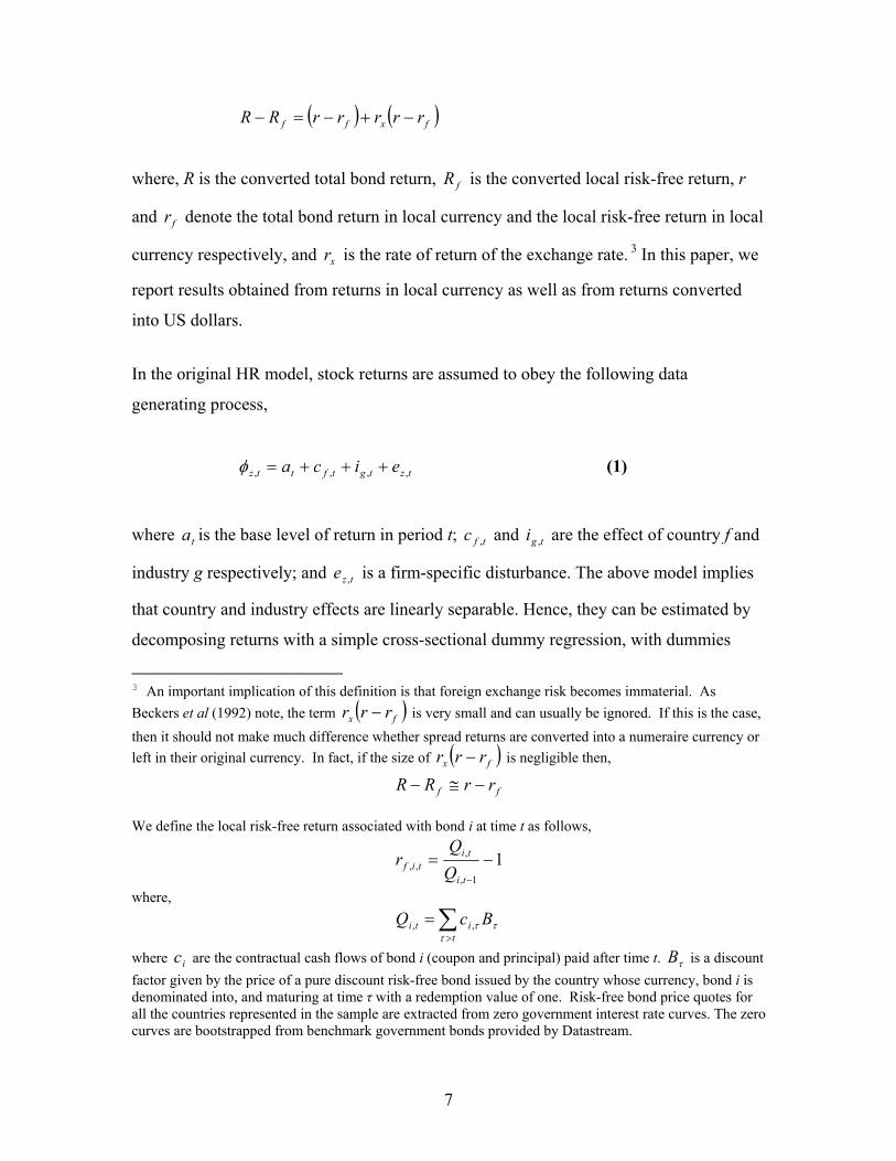
R − R f = (r − r )+ r (r − r )f x f

where, R is the converted total bond return, R f is the converted local risk-free return, r

and rf denote the total bond return in local currency and the local risk-free return in local

currency respectively, and r is the rate of return of the exchange rate. 3 In this paper, wex

report results obtained from returns in local currency as well as from returns converted

into US dollars.

In the original HR model, stock returns are assumed to obey the following data

generating process,

φ t z = at + c t f + i t g + e t z (1), , , ,

where at is the base level of return in period t ; c ,t f and i t g , are the effect of country f and

industry g respectively; and e t z is a firm-specific disturbance. The above model implies ,

that country and industry effects are linearly separable. Hence, they can be estimated by

decomposing returns with a simple cross-sectional dummy regression, with dummies

3 An important implication of this definition is that foreign exchange risk becomes immaterial. As Beckers et al (1992) note, the term r (r − r ) is very small and can usually be ignored. If this is the case, x f

then it should not make much difference whether spread returns are converted into a numeraire currency or left in their original currency. In fact, if the size of r (r − r ) is negligible then, x f

R − R f ≅ r − rf

We define the local risk-free return associated with bond i at time t as follows, Q ,t i r t i f = − 1 , ,

t i −1Q , where,

Q , =∑ ci ,τ Bt i τ τ >t

where ci are the contractual cash flows of bond i (coupon and principal) paid after time t . B τ is a discount factor given by the price of a pure discount risk-free bond issued by the country whose currency, bond i is denominated into, and maturing at time τ with a redemption value of one. Risk-free bond price quotes for all the countries represented in the sample are extracted from zero government interest rate curves. The zero curves are bootstrapped from benchmark government bonds provided by Datastream.

7

capturing the various countries and industries effects represented in the sample. The

regression will look like,

φ = a + c 1Cz 1, + ... + c 9C + I i z 1, + ... + I i z 8 , + e (2)z z 9 , 1 8 z

where upper case letters denote dummies (C and I stand for country and industry

respectively) and lower case letters their coefficients. a is the constant term.

As it stands, the model is not identified because of perfect linear dependence among the

regressors. As suggested by HR, this is solved by imposing linear constraints such that

the weighted sum of the coefficients of each set of dummies is zero,

9 8

∑α c = 0 and ∑β ig = 0 (3)f f gf =1 g =1

where, α f and β g are the market value weights of country f and industry g and

α f = β g = 1 . Such restrictions are appealing for two reasons: ∑ f ∑ g

(i) They allow for a more immediate interpretation of the meaning of dummies’

coefficients. In every group of dummies, each dummy captures deviations of the

dependent variable from the dependent variable’s cross-sectional unconditional

mean, which corresponds to the regression constant. This is useful because the

regression constant has an appealing economic meaning as the mean return of the

international market. Therefore, country, industry and other dummies’ coefficients

describe the cross-sectional behaviour of returns in a particular country, industry or

of particular bond characteristics as deviations from the average international

market return.

(ii) The second interesting implication that follows from the restrictions is that they

provide a simple way to model, and hence understand, the effect of diversification

on portfolio returns. Through diversification, portfolio returns lose the source of

8

variation stemming from the dimension being diversified (e.g. the country

dimension). For example, by virtue of (3), the return of a portfolio that is

geographically diversified will not have a country effect. Therefore, portfolio risk

can be seen as composed by a core element that cannot be diversified away, i.e. the

volatility of the market as a whole, plus additional sources of volatility that arise

because of the differing composition of the portfolio relative to the market. The

former type of risk is ‘globally’ systematic whereas the latter types are only

‘locally’ systematic because they can be eliminated by increasing asset diversity in )the portfolio.(4

We extend the HR model in two ways: (a) To broaden its applicability to bond returns

and, (b) to measure the impact of national industry diversification. The former extension

is simply obtained by adding maturity, seniority and rating effects to the data generating

process. This implies that new dummies are included in equation (2). Three maturity

dummies separate bonds with maturities up to 2 years, from 2 to 5 years and above 5

years. Similarly, we distinguish between senior and junior bonds as well as AAA, AA, A

and BBB rated bonds. The inclusion of these dummies is consistent with Fama and

French (1993) who find that bond returns are affected by both maturity and default risk

factors.

The latter extension is implemented by replacing global industry effects with national

industry effects in the data generating process. a + i in the HR model represents a global

industry factor diversified across countries. One way to measure benefits of cross­

industry diversification is to see how much, on average, the volatility of a + i falls when

industry effects are diversified away, which results in the industry effect i to disappear

due to constraints (3). With the introduction of national industries we shall be able to

measure the diversification benefits that come from cross-industry as well as same­

industry diversification. Again the gain can be measured by the drop in volatility from

(4) The difference between idiosyncratic risk and ‘locally’ systematic risk is that the former can be decreased by simply increasing the number of assets in the portfolio regardless of their characteristics (ie country of issue, industry, maturity), while the latter can only be diminished through diversification by asset characteristic.

9

a + i to a where i this time represents a national industry effect.5 We will show that part

of the volatility reduction of geographical diversification is due to national industry

effects. Hence, portfolio managers should be as discriminating in selecting national

industries as they are in selecting countries when devising their investment policy. The

right choice of sectors will allow them to maximise the benefits of country

diversification.

The introduction of national industry effects leads to an interesting statistical problem,

which relates to how perfect collinearity should be dealt with in regression (2). The group

of national industry dummies for one country are perfectly collinear with the dummy for

that country. This implies that we need as many restrictions on industry dummy

coefficients as there are countries. These are implemented by adjusting the coefficients of

the industry dummies associated with any given country so that they can be interpreted as

deviations from the country’s return effect rather than the global market return as one

would normally do. The procedure to achieve this is summarised in Appendix B.

We estimate regression (2) for each month in the sample period using weighted least

squares. Bonds and stocks are value weighted. The value of a bond at a particular date is

its amount outstanding in US dollars at that date, while the value of a stock is the market

capitalization of its issuer in US dollars.

3.1. Global and national industry effects

How would the introduction in (2) of both global and national industry dummies

influence our estimations? Do global and national industry dummies capture different

effects? To answer these questions we have considered a simple example reported in

Table 3. The example shows that the volatility of national industry effects when

estimated alone is distributed between the national and global industry effects when they

are jointly estimated, without any addition or diminution. Essentially, global industry

effects capture the common variation of national industries within a particular global

5 Measures of diversification gains will be formally discussed in Section 4.

10

sector, but do not add explanatory power. Therefore, it is not necessary to estimate global

industry effects when national industries are used. The extended HR model presented in

this paper encompasses the standard HR model. In the Table, we show three examples in

which global industries, when estimated in combination with national industries absorb

no, some or the whole volatility (Panel A, B and C respectively) of stand-alone national

industry effects.

4. Interpretation of models’ output

One of the main indicators of country and industry diversification used in the literature

based on the HR model6 is the average variance of the estimated dummy coefficients c ˆ

and i in (2), that is, the portion of return that can be attributed to country and industry

effects respectively. We call this the return effect variance indicator (REVI).

In this section, we show that the REVI can lead to overestimation of diversification

effects when the “pure”7 factors, a ˆ + c ˆ and a ˆ + i have non homogenous volatility. Let us

illustrate the problem with an example. Consider two groups of assets with return

X i for i = ,...,1 nX and Yi for i = ,...,1 nY . Each group is influenced by a different return

effect (e.g. a country effect). Then, we could use the HR model and the REVI to measure

the diversification gain one achieves by combining the two groups of assets in a portfolio.

First, we will need to estimate the following regression:

ri = a + F f X i + F f Y i + ei (4)X , Y ,

where ri = X i for i = ,...,1 nX and ri = Yi for i = nX + ,...,1 N , N = nX + nY , F X i and ,

F Y i are dummies that takes a value of 1 when ri is a return from the first or second group ,

6 Heston and Rouwehorst (1994,1995), Griffin and Karolyi (1998), Baca, Garbe and Weiss (2000), Cavaglia, Brightman and Aked (2000) and Isakov and Sonney (2003) among others. 7 HR name these indices “pure” because they represent the return within a particular country or industry without any industry or country effects respectively.

11

of assets respectively, and a value of zero otherwise. With equal weighting and the usual

constraints, the ordinary least square estimates8 of a , f X and fY will be,

N

Na ˆ =

1 ∑ ri = nX X +

nY Yi = 1 N N

ˆ nX

a ˆn

f X = 1 ∑ X i = −

nY ( X − Y )X i = 1 N

ˆ nY

a ˆ nXfY = 1 ∑ Y = − ( Y − X )in Y i = 1 N

nX nY1n

where X = ∑ X i and Y = 1 ∑ Yi . It follows that the variance of the two return

X i = 1 nY i = 1

effects f X and f Y is given by,

2 2 2 2 2f V ˆ S( )= k (σ +σ Y − 2 ρ σ σ )≥ k (σ −σ ) (5)S X X Y S X Y

where k =

N − nS 2

, σ is the volatility of factor X and σ is the volatility of factor Y N

X

Y, ρ is the correlation between factor X and Y and s = X ,Y . The REVI will then be

nY ( REVI = nX ( ) f V ˆ

X + f V Y ) (6)N N

With factor correlation equal to 1, one would expect a correct measure of diversification

to be zero, as there are no diversification gains from combining in the same portfolio the

two groups of assets. However, as it can be easily seen from (5) and (6) this is only the 2case if the two factors have identical variance, σ = σ Y

2 . As the difference in varianceX

8 Here, to keep the analysis simple, we use equal weights and ordinary least squares unlike in the rest of the paper. Using value weights and weighted least squares would only complicate the notation without adding insight.

12

increases, again with ρ = 1, so does the REVI. This follows because the lower bound of

( f V ˆ S ), that is the right hand side of the inequality in (5), grows as σ −σ increases.X Y

Therefore, the REVI increasingly over-estimates diversification gains the larger the

dispersion of factor variance. Thus, we need to devise another indicator of diversification

effects.

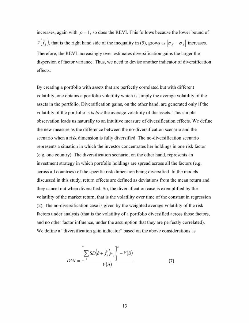
By creating a portfolio with assets that are perfectly correlated but with different

volatility, one obtains a portfolio volatility which is simply the average volatility of the

assets in the portfolio. Diversification gains, on the other hand, are generated only if the

volatility of the portfolio is below the average volatility of the assets. This simple

observation leads us naturally to an intuitive measure of diversification effects. We define

the new measure as the difference between the no-diversification scenario and the

scenario when a risk dimension is fully diversified. The no-diversification scenario

represents a situation in which the investor concentrates her holdings in one risk factor

(e.g. one country). The diversification scenario, on the other hand, represents an

investment strategy in which portfolio holdings are spread across all the factors (e.g.

across all countries) of the specific risk dimension being diversified. In the models

discussed in this study, return effects are defined as deviations from the mean return and

they cancel out when diversified. So, the diversification case is exemplified by the

volatility of the market return, that is the volatility over time of the constant in regression

(2). The no-diversification case is given by the weighted average volatility of the risk

factors under analysis (that is the volatility of a portfolio diversified across those factors,

and no other factor influence, under the assumption that they are perfectly correlated).

We define a “diversification gain indicator” based on the above considerations as

2 (ˆ ˆ ( )∑ a SD + f j )w − a V ˆj

DGI = j

( ) (7)

a V ˆ

13

where SD and V denote the standard deviation and variance operators and wi is the time

average weight for factor i . Standard deviation and variance are calculated from the time

series of a ˆ and f j obtained by estimating cross-section (4) at different times over the

sample period. It is easy to see that this measure, unlike the REVI, is zero in the case of

perfect correlation between a + f and a ˆ + f 2 , and increasing as the correlation between 1

the two indices decreases, which is what we would expect from a suitable indicator of

portfolio diversification. For instance, in our example with two groups of assets, the DGI

would be

2σ X σ nX nY ( 1 − ρ)Y 2

DGI = N V ( ) a ˆ

The desirable properties of this indicator can be easily summarised. If ρ = 1, the DGI

equals zero regardless of the difference between σ and σ Y . If ρ < 1 and σ X −σX Y

increases but factor covariance remains constant, that is σ X σ does not change, thenY

the numerator of the DGI remains unaltered. The denominator, V ( a ˆ) , will grow because

the minimum volatility achievable with total diversification has gone up. So the final

effect would be a decline in DGI. The above conditions apply to the REVI, on the other

hand, would make it go up, which is misleading as the difference in variance between the

no-diversification and the diversification scenarios has remained the same. To conclude,

the DGI appears to be a superior diversification indicator in the general case when risk

factors in the portfolio have heterogeneous volatility.

4.1 Asymptotic DGI

The DGI as defined in (7) is based on the assumption that the number of assets used to

estimate each return effect f S is sufficiently large as to eliminate from the estimate the

impact of idiosyncratic risk. Factors that are poorly populated will have an inflated

14

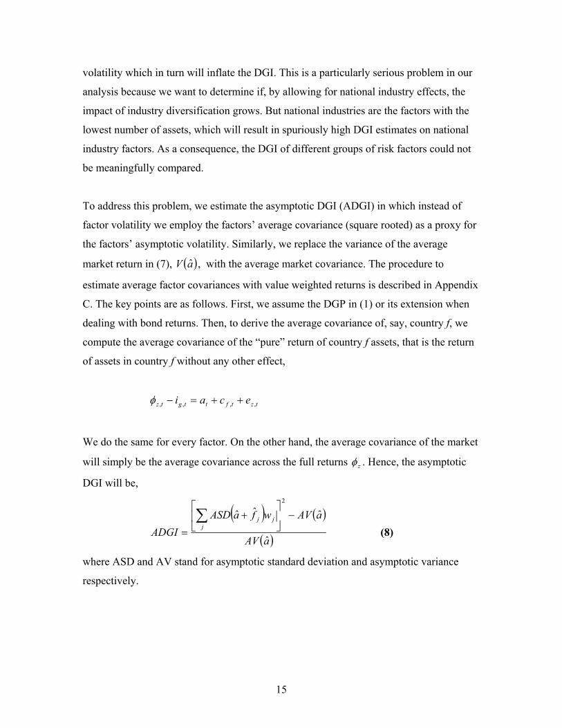
volatility which in turn will inflate the DGI. This is a particularly serious problem in our

analysis because we want to determine if, by allowing for national industry effects, the

impact of industry diversification grows. But national industries are the factors with the

lowest number of assets, which will result in spuriously high DGI estimates on national

industry factors. As a consequence, the DGI of different groups of risk factors could not

be meaningfully compared.

To address this problem, we estimate the asymptotic DGI (ADGI) in which instead of

factor volatility we employ the factors’ average covariance (square rooted) as a proxy for

the factors’ asymptotic volatility. Similarly, we replace the variance of the average

market return in (7), V (a ), with the average market covariance. The procedure to

estimate average factor covariances with value weighted returns is described in Appendix

C. The key points are as follows. First, we assume the DGP in (1) or its extension when

dealing with bond returns. Then, to derive the average covariance of, say, country f, we

compute the average covariance of the “pure” return of country f assets, that is the return

of assets in country f without any other effect,

=φ t z − i t g at + c t f + e t z , , , ,

We do the same for every factor. On the other hand, the average covariance of the market

will simply be the average covariance across the full returns φ . Hence, the asymptotic z

DGI will be, 2

∑ a ASD + f j )w j − a AV ˆ(ˆ ˆ ( )

ADGI = j

( ) (8)

a AV ˆ

where ASD and AV stand for asymptotic standard deviation and asymptotic variance

respectively.

15

5. Results

Results have been derived with local currency returns as well as with returns converted in

US dollars. The advantage of the former approach is that local currency returns are more

insulated against foreign exchange risk.9 This has important implications when studying

bond portfolio returns. As foreign exchange risk tends to inflate the importance of

country diversification, that effect alone may be responsible for changes in the relative

size of country as opposed to industry diversification in bond portfolios. Equity returns,

on the other hand, are much larger than bond returns and we find that the marginal effect

of currency risk on them is small and unlikely to influence the ranking of alternative

diversification effects. We also derive results after converting returns in US dollar for

ease of comparison of our findings with previous studies, which often use common

currency returns, and to show the effect of geographical and industrial diversification

when currency risk is left unhedged.

Table 4 and 5 report descriptive statistics of our stock and bond samples with value

weighted local currency monthly returns.10 The HR model applied to stocks leads to an

average country factor volatility and correlation of 3.907% and 0.475 respectively. The

average volatility of global industry factors is lower at 3.456% while the correlation is

substantially higher at 0.649. When industry and country factors are diversified they will

yield the same portfolio volatility equal to the volatility of the global market return a .

Therefore, according to the HR model, from this preliminary analysis, one could

tentatively conclude that country diversification is more effective in reducing portfolio

risk because it brings about a larger drop in portfolio volatility (which can be inferred

from the larger value of country factor volatility). However, when using the extended HR

model we reach the opposite conclusion. Average national industry factor volatility is

9 As Dumas and Solnik (1995) point out local currency returns are not fully free from currency effects as they still include a currency premium. 10 Descriptive statistics tables with dollar denominated returns have not been included for brevity and can be obtained from the author on request. Dollar stock returns statistics are qualitatively similar to those in Table 4. Dollar denominated bond factor total returns are much more volatile than the local currency ones due to currency risk (which is more noticeable than in stock factors for the smaller magnitude of bond returns). Also, the average correlation of bond total returns of country factors denominated in US dollars is noticeably lower compared with the average local currency country factor return correlation.

16

higher and its correlation lower than those of country factors. But, as pointed out in

Section 4.1, national industry factors are internally much less diversified than all the other

factors. This implies that their volatility is affected to a greater extent by idiosyncratic

risk. So, a firm conclusion about the relative efficacy of country and industry

diversification in the stock market can not be reached from this Table. The problem of

idiosyncratic risk in factors is directly addressed in Tables 6 to 8 through the calculation

of asymptotic diversification gain indicators.

In Table 5, we report the mean, volatility and correlation of bond total return and spread

return for the various factors estimated with the HR and ExHR models. The models yield

comparable results for all but industry factors. Also, factor correlations are generally

lower for spread returns than for total returns. Interestingly, this implies that interest rate

risk is less diversifiable than spread risk. As expected, the ExHR model produces national

industry factors that are more volatile (and less correlated) than the global industry

factors obtained from the HR model. Both models lead to plausible maturity factors for

total and spread returns, with increasing factor mean and volatility as maturity increases.

Results for seniority factors, on the other hand, are more surprising. Both the total and

spread returns of the senior bond factor have slightly higher mean than the junior bond

factor, although we expect the risk premium of senior bonds to be lower. This curious

finding is consistent with Fridson and Garman (1997) who show that senior bonds have

higher risk premiums than subordinated bonds within the same rating category. The

explanation for this result lays in the fact that rating agencies tend to give senior issues a

higher rating than junior issues from the same issuer. So, within a particular rating, say A,

one can find senior bonds with a probability of default higher than a typical A-rated

security because issued by companies with lower rating (i.e. BBB), and junior bonds with

lower probability of default because issued by A-rated companies. As a result, the

expected loss at default defined as the product between default probability and expected

recovery rate may be higher for senior than for junior bonds, thus justifying the higher

return of senior bonds.

17

Another interesting “anomaly” is the total return volatility of rating factors. BBB-rated

bonds exhibit a lower volatility than all the more highly rated issues. The total return

volatility of a rating factor depends on the volatility of interest rates, the volatility of

spreads and the correlation between spreads and interest rates. Our finding can be

explained by the negative correlation between corporate bond yield spreads and Treasury

yields, discussed in Duffee (1998), which may be stronger for lowly rated issues. This

interpretation of the results is confirmed by the volatility of spread returns – also reported

in the Table - which, as common sense suggests, is increasing as the rating worsens.

In Tables 6, 7 and 8 we report the two measures of diversification gains discussed in

previous sections, the REVI and the ADGI, for equity and bond portfolio returns. One of

the main findings, is that industry effects appear to be more important than the standard

HR model would allow one to infer. A comparison between the REVI and the ADGI

shows that the new measure reveals significantly larger industry diversification effects.

This increase, relative to country diversification, is by a factor of 1.61 (1.83) from 0.41

(0.30) to 0.66 (0.54).

With the introduction of national industry effects, local currency (US dollar)

diversification gains, as measured by the ADGI, relative to country diversification, rise

by a factor of 1.88 (1.92) from an industry over country ADGI ratio of 0.35 (0.28) to one

of 0.66 (0.54) in the stock portfolio (Table 6). In the bond market, the increase in the

ratio is by a factor of 5.71 (2.99) from 0.10 (0.12) to 0.57 (0.35) for total returns (Table

7). For spread returns (Table 8) the increase is smaller and equal to 1.34 (1.32) from 0.36

(0.35) to 0.48 (0.46).

The more striking difference between the REVI and the ADGI occurs when we look at

maturity diversification effects in Table 7. When local currency returns are used with the

ExHR (HR) model the REVI shows that maturity diversification is 2.10 (2.17) times

more effective in reducing portfolio risk than country diversification. The ADGI based

maturity to country ratio is 0.15 (0.15), which leads to the opposite and correct

conclusion. As pointed out in Section 4, the difference is due to the wide variation in the

18

volatility of maturity factors which inflates the REVI. A discrepancy of such magnitude

is not observed for other groups of factors (industry, seniority and rating factors for

example), because the volatility of factors in non-maturity groups is normally much less

erratic. When bond total returns are denominated in US dollar, the ratios are overall more

aligned and the odd spike in the REVI based maturity/country ratios disappears, as

country effects become more prominent because of currency risk.

The ranking in diversification effect on bond portfolio total return (in local currency) that

emerges by looking at the ExHR model in Table 7, places in the first position country

diversification, followed by industry diversification which is 43% less powerful, and by

maturity diversification, 85% weaker. Seniority and rating diversification do not have any

significant impact on portfolio risk as measured by the ADGI. The slightly negative

ADGI for rating factors is due to the fact that estimated rating return effects are very

small (with an estimated variance of one half a basis point, see column 3 in Table 7).

Therefore, if rating effects are negligible the average covariance among bonds within a

particular rating is not distinguishable from the average covariance across the whole

portfolio. The asymptotic ADGI which compares the two covariances should then be zero

or marginally deviate from zero in excess or defect, as the results indicate.

Results for bond spreads in Table 8 are not dissimilar from those for total returns. Again

the ranking of diversification effects as measured by the ADGI sees country

diversification first followed by industry diversification which is 52% less powerful with

local currency spreads (54% with US dollar spreads) and by maturity factors, 71% (71%)

weaker. Rating diversification brings about a diversification gain which is 16% (16%) of

that of country diversification while the relative strength of seniority diversification is

negligible. The ADGI of national industry factors reported in the Table have been

computed by assuming the average covariance in each national industry to be positive or

zero, which is a condition that must hold asymptotically, that is when the number of

securities is large.11 Indeed, while this assumption is not needed for all other factors as

11 The minimum average correlation of a portfolio tends to zero from below as the number of assets increases. Formally, given a portfolio of n equally weighted assets, with constant asset variance and

19

they normally include a sufficiently high number of securities, some national industries

are poorly populated which, together with the modest size of the average spread return,

may cause their average covariance to become negative and result in the computation of

the ADGI being not feasible.

6. Conclusion

Several papers have looked at the relative importance of country and industry

diversification in international portfolios of stocks. Here we critically appraise previous

contributions and point out that industry effects on portfolio diversification have been

underestimated. We correct for the estimation bias and conclude that overall industry

diversification may have a much stronger impact on portfolio risk than previously

believed. In addition, we find that the results from existing models in the literature need

to be interpreted with caution, especially when a popular indicator is used to measure

diversification effects. We show that when risk factors in the portfolio have

heterogeneous volatility such indicator will spuriously inflate causing an over-estimation

of diversification gains. We suggest a new indicator that addresses this problem. Finally,

we extend previous studies’ analysis of country and industry diversification in stock

portfolios, by looking at the determinants of diversification in corporate bond portfolios

which, to the best of our knowledge, is the first attempt in this direction. From our bond

sample we detect smaller diversification benefits from geographical and industrial

diversification than in the stock market, after controlling for maturity, seniority and rating

influences.

constant correlation ρ , for portfolio volatility to be positive the following condition must be satisfied,

1 − 1ρ − > ( n − ) .

20

Appendix A

The following seniority types are listed roughly in decreasing order or repayment priority.

Senior liquidation status types:

1. Collateralised: Collateralised debt is secured by specifically allocated assets

including financial instruments, property, equipment, held in trust.

2. Guaranteed: Guaranteed debt is accompanied by a pledged guarantee of

(re)payment of interest and/or principal by a non-sovereign government issuer and/or

other entity or entities.

3. Mortgage: The issuer has provided an unspecified lien to the bondholders on his

properties to satisfy any unpaid obligation.

4. Secured: Secured means that additional security is provided for payment of

interest and principal.

5. Senior proper: Denotes an unsecured issue ranked higher than ‘unsecured’ issues.

Junior liquidation status types:

1. Unsecured: Unsecured means that no provision is made for additional security

enhancement. An ‘unsecured’ security type is ranked higher than any subordinated

security types.

2. Subordinated: Denotes issues ranked below ‘unsecured’ issues.

Source: Reuters 3000 Fixed Income Services.

21

Appendix B

The procedure to estimate the extended HR model involves imposing restrictions to

regression coefficients in a sequential way. The general regression we want to estimate at

time t is (the subscript t is not included in expressions below to simplify notation):

N N M λ

φ = a +∑ C c λ +∑∑ I i γλ + eλ γλ ,,λ= 1 λ= 1 γ = 1

where I γλ and i γλ are respectively the dummy and its coefficient for industry γ in , ,

country λ . The estimation procedure consists of the following three steps. N M λ

Step 1. Since ∑ C is equal to the constant vector and ∑ I γλ = C λ , to avoidλ , λ= 1 γ = 1

multicollinearity we need to eliminate one country and one industry sector in each

country. The eliminated coefficients will be reintroduced after estimation as described in

Step 2 and 3. Then, the regression becomes,

N − 1 N M λ − 1

φ = a +∑ C c λ +∑ ∑ I i γλ + eλ γλ ,,λ= 1 λ= 1 γ = 1

Step 2. We now impose restrictions on the remaining national industry coefficients that

will allow us to reintroduce the lost coefficients. To do so, we add a constant kλ to all the

estimated coefficients of the industries in country λ , for any λ , such that M λ

− 1∑( i , + v k γλ = 0 , where v ,λ ) γλ = w γλ w λ with w γλ denoting the relative weight ofγλ , , , γ = 1

N M λindustry γ in country λ over the cross-sectional sample ∑∑ w = 1

, and w λ,γλ

λ= 1 γ = 1

Nindicating the relative weight of country λ over the cross-sectional sample ∑ w λ = 1 . λ= 1

Note that iλ ,M λ is equal to zero for all λ due to restrictions in the previous step. It follows

22

M λ

ˆthat k λ − = ∑ v i , for λ =1,…,N. Next, country and industry coefficients are re-defined ,γλ γλ γ = 1

as

*i γλ = i γλ + k λ For λ =1,…,N and γ = 1,…,Mλ -1 , ,

*

ˆ

i λ ,M λ= kM λ

For λ =1,…,N

*c λ = c ˆλ − k λ For λ =1,…,N-1

* c ˆλ − = k λ For λ =N

Note that, at this stage, the restrictions on national industries do not affect the regression

constant.

Step 3. We now implement restrictions in country coefficients. Similarly to the previous N

* *step, the objective is to ensure that ∑( c ˆλ + w k = 0 which implies k − = ∑ w c . Then,) λ

N

ˆλ λ λ= 1 λ= 1

country coefficients and the regression constant are redefined as,

ˆ ** ˆ* c λ = c λ + k For λ =1,…,N

a ˆ* = a ˆ − k

** *The new coefficients a ˆ* , c ˆλ and i γλ will guarantee that the following relations hold, ,

N ** i. ∑ w c λ = 0ˆλ

λ= 1

M λ *ˆii. ∑ v i γλ = 0 for λ :1,…,N.γλ ,,

γ = 1

In addition, if we use weighted least squares to estimate the regression above then,

23

iii. a* is the unconditional weighted average return at time t.

** iv. a* + cλ is the unconditional weighted average return of country λ at time t.

** * v. a* + cλ + i is the unconditional weighted average return of industry γ in countryλ ,γ

λ at time t.

The procedure does not depend on the presence of other variables (dummies or

otherwise) in the regression so it can be easily extended to the model employed for the

analysis of bond returns.

Appendix C

We estimate index asymptotic variances as follows. Let Rt and µ be the return of an

index and its mean, Rit the return of asset i included in the index, wit the weight of asset i

at time t and T the number of return observations. If a security’s return is not available at

any given time its weight for that date is set to zero. Then, the variance of the index can

be decomposed as

T 1 T N 21 ∑(R − µ)

2

= ∑ ∑ w R it − µ

= T −1 t =1

t T −1 t =1

i=1 it

1 T N N 2

∑∑( w R − µ w )+∑µ w − µ =i itT −1 t =1 i=1 it it i it

i=1

1 T N 2

−∑ ∑(R − µ )w + ( µ µ ) = tT −1 t =1

i=1 it i it

N N 2 2∑(R − µ ) wit +∑(R − µ )(R − µ ) w w + T it i jt j it jt1 ∑

i=1 it i

i≠ j N

− 2T −1 t =1 2∑(R − µ µ µ )w + ( µ µ )

it i )( t − it t i=1

24

Note that,

N 1 T 2 2a) ∑ ∑( R − µ ) wit is similar to the weighted sum of the variances of the

i= 1 T − 1 t = 1 it i

assets in the index with the difference that the weights here are time dependent. In 2fact, the unusual term (µ − µ) is caused by the variability of asset weights over t

time.

N 1 T

b) ∑ ∑( R − µ )( R − µ ) w w jt is approximately equal to the weighted j iti≠ j T − 1 t = 1

it i jt

sum of all covariances. The asymptotic covariance is defined as TN 1 * * * wit∑ ∑( R − µ )( R − µ ) w w jt where wit =

i≠ j T − 1 t = 1 it i jt j it N .

∑ w w jtit i≠ j

N 1 T

)( −c) 2∑ ∑( R − µ µ µ ) w is approximately equal to the weighted sum iti= 1 T − 1 t = 1

it i t

of covariances between asset returns and the cross-sectional mean.

T

d) 1 ∑( µ µ ) is the variance of the cross-sectional mean. − T 1

− 2

t = 1 t

As the number of assets increases a) and c) tend to zero while b) tends to the asymptotic

covariance. d) is negligible for all index variance decompositions reported in the paper.

Therefore, the asymptotic variance of an index is typically well approximated by the

index’s asymptotic covariance.

25

References

Baca S. P., B. L. Garbe and R. A. Weiss (2000) ‘The rise of sector effects in major

equity markets.’ Financial Analysis Journal 56, October, pages 34-40.

Beckers, S., R. Grinold, A. Rudd and D. Stefek (1992) ‘The Relative Importance Of

Common Factors Across The European Equity Markets,’ Journal of Banking and

Finance, v16(1), pp. 75-96.

Cavaglia S., C. Brightman and M. Aked (2000) ‘The increasing importance of industry

factors.’ Financial Analysis Journal 56, pages 41-54.

Drummen, M. And H. Zimmermann (1992) ‘The Structure of European Stock

Returns,’ Financial Analysts Journal 48, pages 15-26.

Duffee, G. R. (1998) ‘The Relation Between Treasury Yields And Corporate Bond Yield

Spreads,’ Journal of Finance, 1998, v53(6,Dec), pages 2225-42.

Dumas, B. and B. Solnik (1995) ‘The World Price Of Foreign Exchange Risk,’ Journal

of Finance, v50(2), pp. 445-479.

Elton, E. J., M. J. Gruber, D. Agrawal and C. Mann (2001) "Explaining The Rate Of

Spread On Corporate Bonds," Journal of Finance, v56(1,Feb), pages 247-277.

Eichholtz, P. M. A. (1996) ‘Does International Diversification Work Better For Real

Estate Than For Stocks And Bonds?,’ Financial Analysts Journal, v52(1,Jan-Feb), 56-62.

Fama, E and French, K (1993), ‘Common risk factors in the returns on stocks and

bonds’, Journal of Financial Economics, Vol. 33, pages 3–57.

Fridson, M. S. and M. C. Garman (1997) ‘Valuing like-rated senior and subordinated

debt’, The Journal of Fixed Income, December, pages 83-93.

26

Grauer, R. R. and N. H. Hakansson (1987) ‘Gains From International Diversification:

1968-85 Returns On Portfolios Of Stocks And Bonds,’ Journal of Finance, v42(3), pp.

721-739.

Griffin, J and Karolyi, A (1998), ‘Another look at the role of the industrial structure of

markets for international diversification strategies’, Journal of Financial Economics, Vol.

50, pages 351–73.

Grubel, H (1968), ‘Internationally diversified portfolios: welfare gains and capital

flows’, American Economic Review, Vol. 58, pages 1,299–314.

Heston, L S and G K Rouwenhorst (1994), ‘Does industrial structure explain the

benefits of international diversification?’, Journal of Financial Economics, Vol. 36, pp.

3–27.

Heston, L. S. and G K Rouwenhorst (1995) ‘Industry And Country Effects In

International Stock Returns,’ Journal of Portfolio Management, v21(3), pp. 53-58.

Hunter, D. M. and D. P. Simon (2004) ‘Benefits Of International Bond Diversification,’

Journal of Fixed Income, , v13(4,Mar), 57-72.

Ibbotson, R. G., R. C. Carr and A. W. Robinson (1982) ‘International Equity and

Bond Returns,’ Financial Analysts Journal, July/August.

Isakov, D. and F. Sonney (2003) ‘Are practitioners right? On the relative importance of

industrial factors in international stock returns’. Working paper, HEC-University of

Geneva.

Kaplanis, E and Schaefer, S (1991), ‘Exchange risk and international diversification in

bond and equity portfolios’, Journal of Economics and Business, Vol. 43, pages 287–307.

Kennedy, P (1986), ‘Interpreting dummy variables’, Review of Economics and

Statistics, Vol. 68, pages 174–75.

27

La Porta, R., F. Lopez-de-Silanes, A. Shleifer and R. W. Vishny (1998) "Law And

Finance," Journal of Political Economy, v106(6,Dec), pp. 1113-1155.

Lessard, D. R. (1974) ‘World, National, And Industry Factors In Equity Returns,’

Journal of Finance, v29(2), pp. 379-391.

Levy, H. and Z. Lerman (1988) ‘The Benefits Of International Diversification In

Bonds," Financial Analysts Journal,’ v44(5), 56-64.

Levy, H and Sarnat, A (1970), ‘International diversification of investment portfolios’,

American Economic Review, Vol. 25, pages 668–75.

Roll, R. (1971) ‘Investment Diversification And Bond Maturity,’ Journal of Finance,

v26(1), 51-66.

Roll, R (1992), ‘Industrial structure and the comparative behavior of international stock

market indices’, Journal of Finance, Vol. 47, pages 3–42.

Solnik, B (1974), ‘The international pricing of risk: an empirical investigation of the

world capital market structure’, Journal of Finance, Vol. 29, pages 365–78.

Suits, D B (1984), ‘Dummy variables: mechanics versus interpretation’, Review of

Economics and Statistics, Vol. 66, pages 177–80.

28

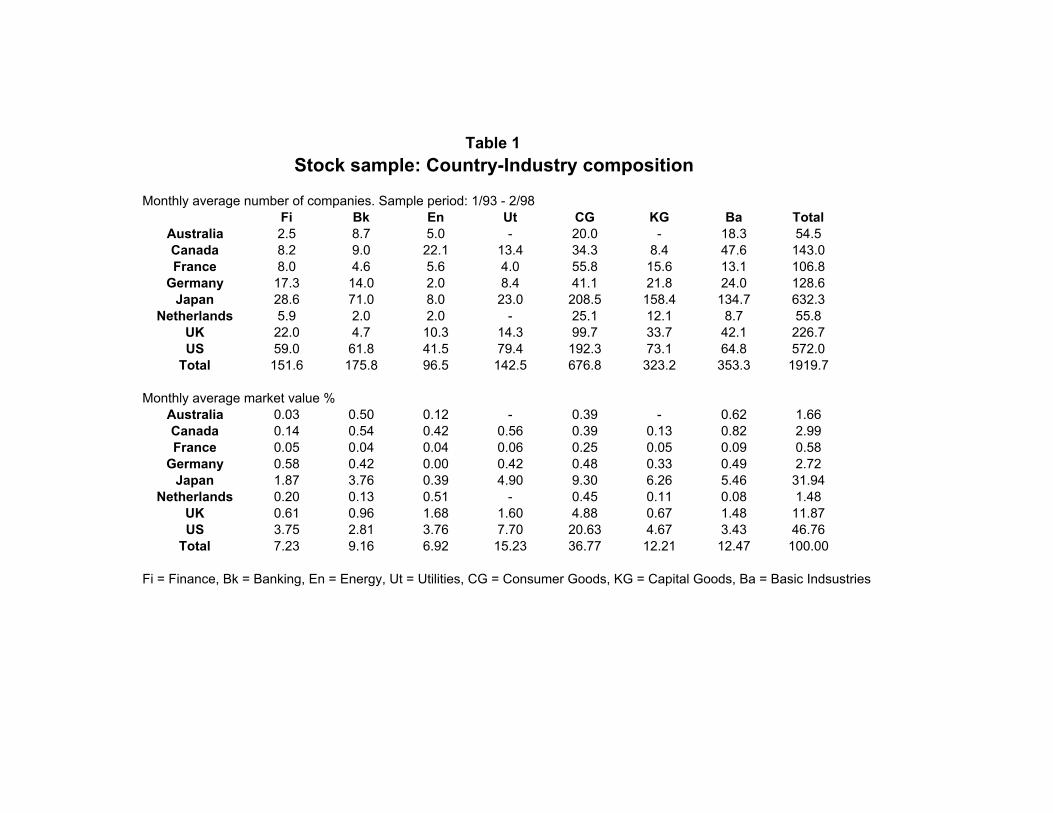
Table 1 Stock sample: Country-Industry composition

Monthly average number of companies. Sample period: 1/93 - 2/98 Fi Bk En Ut CG KG Ba Total

Australia 2.5 8.7 5.0 - 20.0 - 18.3 54.5 Canada 8.2 9.0 22.1 13.4 34.3 8.4 47.6 143.0 France 8.0 4.6 5.6 4.0 55.8 15.6 13.1 106.8

Germany 17.3 14.0 2.0 8.4 41.1 21.8 24.0 128.6 Japan 28.6 71.0 8.0 23.0 208.5 158.4 134.7 632.3

Netherlands 5.9 2.0 2.0 - 25.1 12.1 8.7 55.8 UK 22.0 4.7 10.3 14.3 99.7 33.7 42.1 226.7 US 59.0 61.8 41.5 79.4 192.3 73.1 64.8 572.0

Total 151.6 175.8 96.5 142.5 676.8 323.2 353.3 1919.7

Monthly average market value % Australia 0.03 0.50 0.12 - 0.39 - 0.62 1.66 Canada 0.14 0.54 0.42 0.56 0.39 0.13 0.82 2.99 France 0.05 0.04 0.04 0.06 0.25 0.05 0.09 0.58

Germany 0.58 0.42 0.00 0.42 0.48 0.33 0.49 2.72 Japan 1.87 3.76 0.39 4.90 9.30 6.26 5.46 31.94

Netherlands 0.20 0.13 0.51 - 0.45 0.11 0.08 1.48 UK 0.61 0.96 1.68 1.60 4.88 0.67 1.48 11.87 US 3.75 2.81 3.76 7.70 20.63 4.67 3.43 46.76

Total 7.23 9.16 6.92 15.23 36.77 12.21 12.47 100.00

Fi = Finance, Bk = Banking, En = Energy, Ut = Utilities, CG = Consumer Goods, KG = Capital Goods, Ba = Basic Indsustries

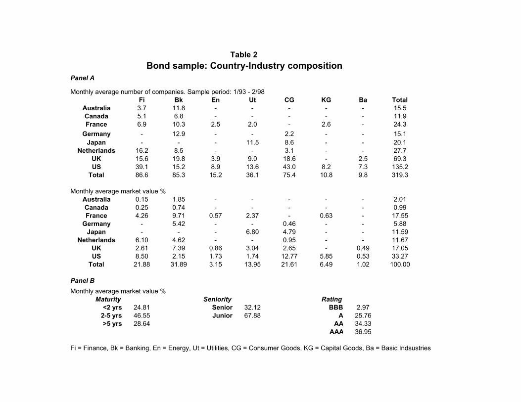
Table 2 Bond sample: Country-Industry composition

Panel A

Monthly average number of companies. Sample period: 1/93 - 2/98 Fi Bk En Ut CG KG Ba Total

Australia 3.7 11.8 - - - - - 15.5 Canada 5.1 6.8 - - - - - 11.9 France 6.9 10.3 2.5 2.0 - 2.6 - 24.3

Germany - 12.9 - - 2.2 - - 15.1 Japan - - - 11.5 8.6 - - 20.1

Netherlands 16.2 8.5 - - 3.1 - - 27.7 UK 15.6 19.8 3.9 9.0 18.6 - 2.5 69.3 US 39.1 15.2 8.9 13.6 43.0 8.2 7.3 135.2

Total 86.6 85.3 15.2 36.1 75.4 10.8 9.8 319.3

Monthly average market value % Australia 0.15 1.85 - - - - - 2.01 Canada 0.25 0.74 - - - - - 0.99 France 4.26 9.71 0.57 2.37 - 0.63 - 17.55

Germany - 5.42 - - 0.46 - - 5.88 Japan - - - 6.80 4.79 - - 11.59

Netherlands 6.10 4.62 - - 0.95 - - 11.67 UK 2.61 7.39 0.86 3.04 2.65 - 0.49 17.05 US 8.50 2.15 1.73 1.74 12.77 5.85 0.53 33.27

Total 21.88 31.89 3.15 13.95 21.61 6.49 1.02 100.00

Panel B Monthly average market value %

Maturity Seniority Rating <2 yrs 24.81 Senior 32.12 BBB 2.97

2-5 yrs 46.55 Junior 67.88 A 25.76 >5 yrs 28.64 AA 34.33

AAA 36.95

Fi = Finance, Bk = Banking, En = Energy, Ut = Utilities, CG = Consumer Goods, KG = Capital Goods, Ba = Basic Indsustries

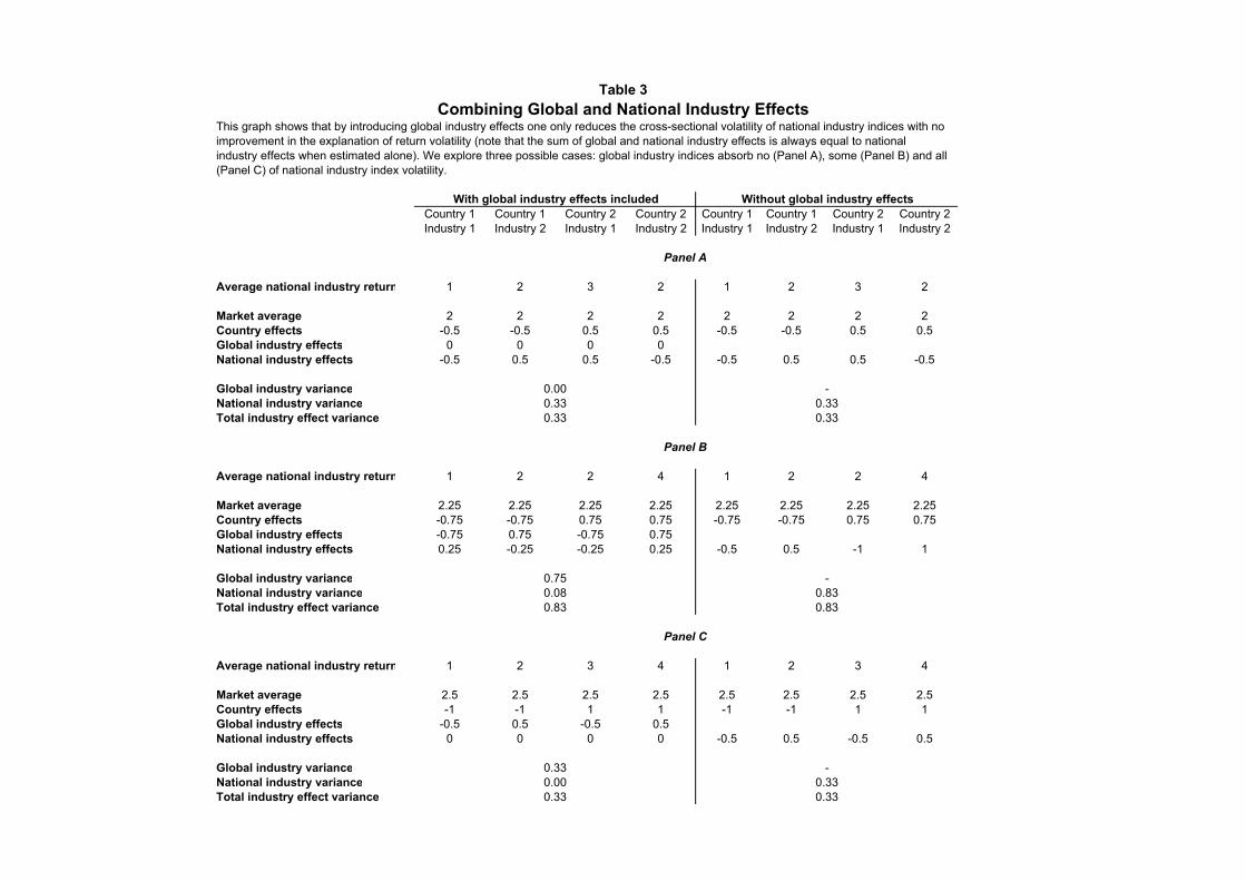
Table 3 Combining Global and National Industry Effects

This graph shows that by introducing global industry effects one only reduces the cross-sectional volatility of national industry indices with no improvement in the explanation of return volatility (note that the sum of global and national industry effects is always equal to national industry effects when estimated alone). We explore three possible cases: global industry indices absorb no (Panel A), some (Panel B) and all (Panel C) of national industry index volatility.

With global industry effects included Without global industry effects Country 1 Country 1 Country 2 Country 2 Country 1 Country 1 Country 2 Country 2 Industry 1 Industry 2 Industry 1 Industry 2 Industry 1 Industry 2 Industry 1 Industry 2

Panel A

Average national industry return 1 2 3 2 1 2 3 2

Market average 2 2 2 2 2 2 2 2 Country effects -0.5 -0.5 0.5 0.5 -0.5 -0.5 0.5 0.5 Global industry effects 0 0 0 0 National industry effects -0.5 0.5 0.5 -0.5 -0.5 0.5 0.5 -0.5

Global industry variance 0.00 -National industry variance 0.33 0.33 Total industry effect variance 0.33 0.33

Panel B

Average national industry return 1 2 2 4 1 2 2 4

Market average 2.25 2.25 2.25 2.25 2.25 2.25 2.25 2.25 Country effects -0.75 -0.75 0.75 0.75 -0.75 -0.75 0.75 0.75 Global industry effects -0.75 0.75 -0.75 0.75 National industry effects 0.25 -0.25 -0.25 0.25 -0.5 0.5 -1 1

Global industry variance 0.75 -National industry variance 0.08 0.83 Total industry effect variance 0.83 0.83

Panel C

Average national industry return 1 2 3 4 1 2 3 4

Market average 2.5 2.5 2.5 2.5 2.5 2.5 2.5 2.5 Country effects -1 -1 1 1 -1 -1 1 1 Global industry effects -0.5 0.5 -0.5 0.5 National industry effects 0 0 0 0 -0.5 0.5 -0.5 0.5

Global industry variance 0.33 -National industry variance 0.00 0.33 Total industry effect variance 0.33 0.33

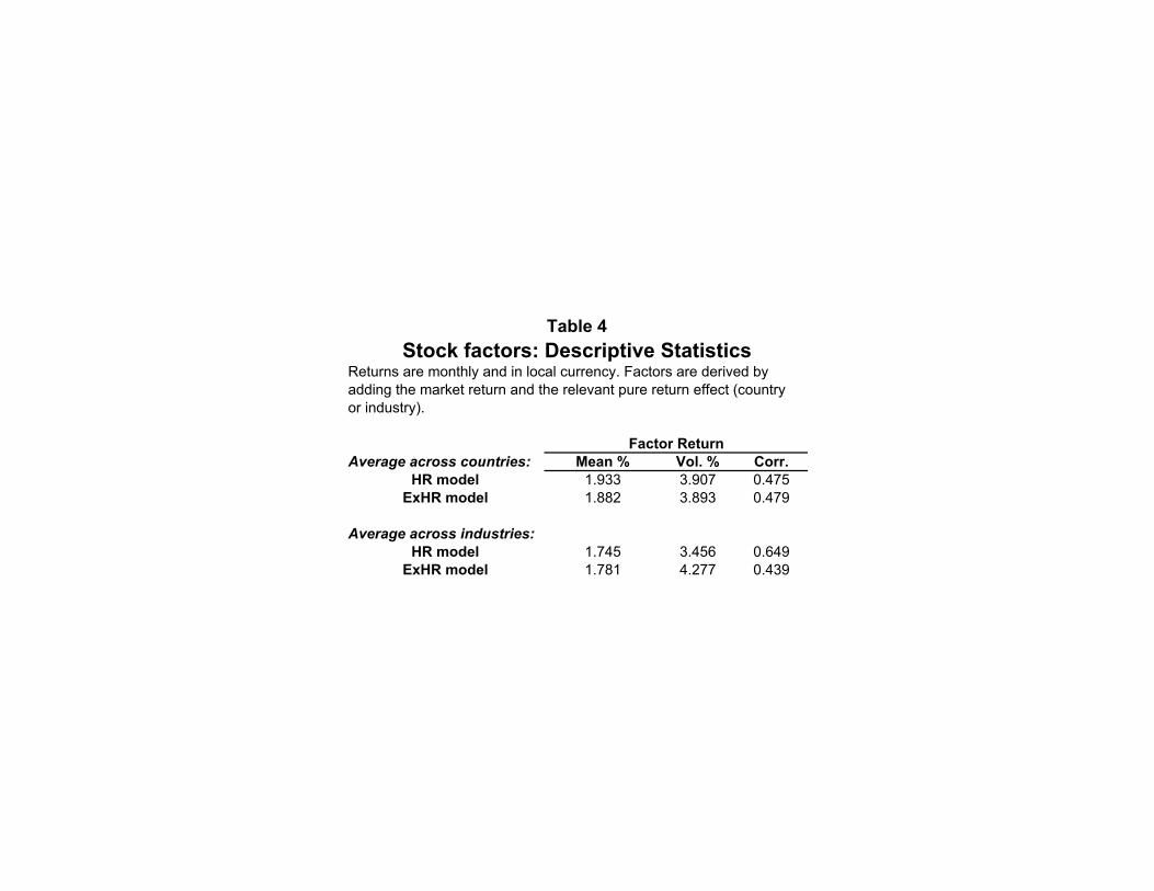
Table 4 Stock factors: Descriptive Statistics

Returns are monthly and in local currency. Factors are derived by adding the market return and the relevant pure return effect (country or industry).

Factor Return Average across countries: Mean % Vol. % Corr.

HR model 1.933 3.907 0.475 ExHR model 1.882 3.893 0.479

Average across industries: HR model 1.745 3.456 0.649

ExHR model 1.781 4.277 0.439

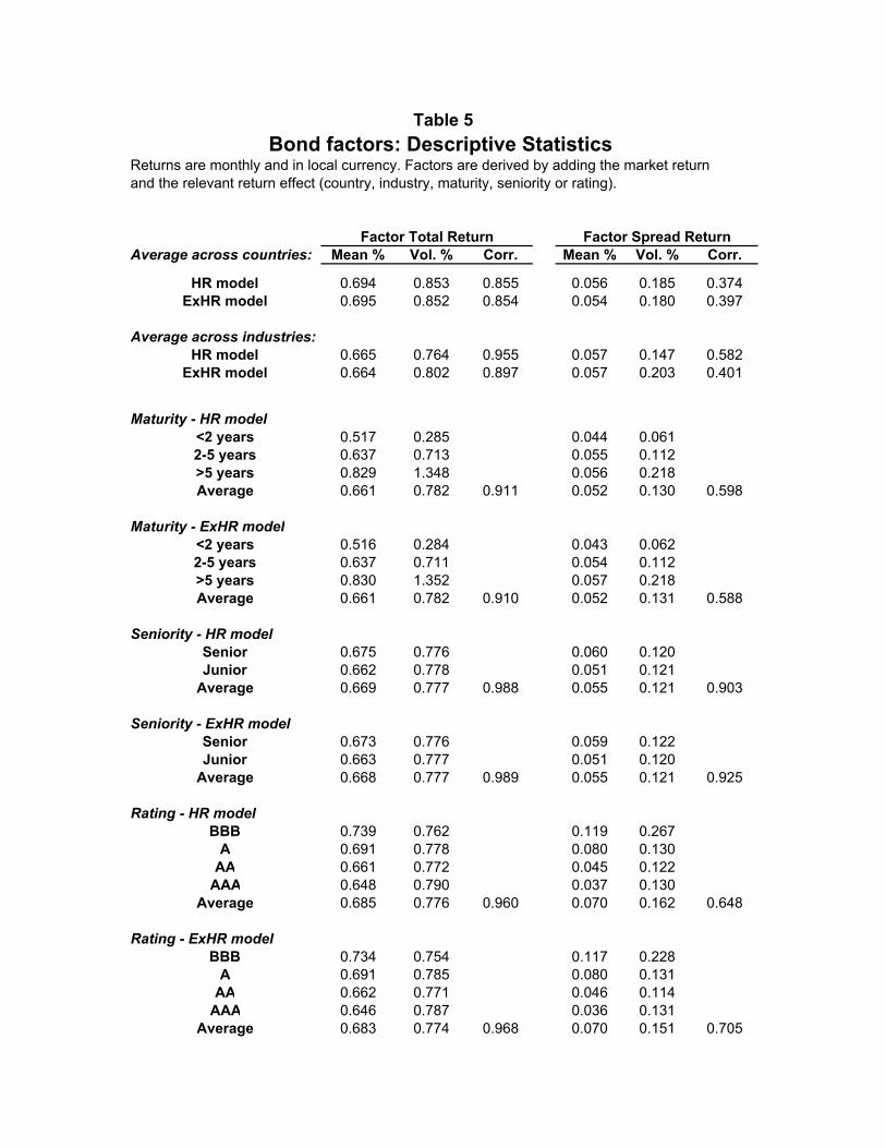
Table 5 Bond factors: Descriptive Statistics

Returns are monthly and in local currency. Factors are derived by adding the market return and the relevant return effect (country, industry, maturity, seniority or rating).

Factor Total Return Factor Spread Return Average across countries: Mean % Vol. % Corr. Mean % Vol. % Corr.

HR model 0.694 0.853 0.855 0.056 0.185 0.374 ExHR model 0.695 0.852 0.854 0.054 0.180 0.397

Average across industries: HR model 0.665 0.764 0.955 0.057 0.147 0.582

ExHR model 0.664 0.802 0.897 0.057 0.203 0.401

Maturity - HR model <2 years 0.517 0.2852-5 years 0.637 0.713>5 years 0.829 1.348Average 0.661 0.782

0.044 0.061 0.055 0.112 0.056 0.218

0.911 0.052 0.130 0.598

Maturity - ExHR model <2 years 0.516 0.2842-5 years 0.637 0.711>5 years 0.830 1.352Average 0.661 0.782

0.043 0.062 0.054 0.112 0.057 0.218

0.910 0.052 0.131 0.588

Seniority - HR model Senior 0.675 0.776 0.060 0.120 Junior 0.662 0.778 0.051 0.121

Average 0.669 0.777 0.988 0.055 0.121 0.903

Seniority - ExHR model Senior 0.673 0.776 0.059 0.122 Junior 0.663 0.777 0.051 0.120

Average 0.668 0.777 0.989 0.055 0.121 0.925

Rating - HR model BBB 0.739 0.762

A 0.691 0.778AA 0.661 0.772

AAA 0.648 0.790Average 0.685 0.776

0.119 0.267 0.080 0.130 0.045 0.122 0.037 0.130

0.960 0.070 0.162 0.648

Rating - ExHR model BBB 0.734 0.754

A 0.691 0.785AA 0.662 0.771

AAA 0.646 0.787Average 0.683 0.774

0.117 0.228 0.080 0.131 0.046 0.114 0.036 0.131

0.968 0.070 0.151 0.705

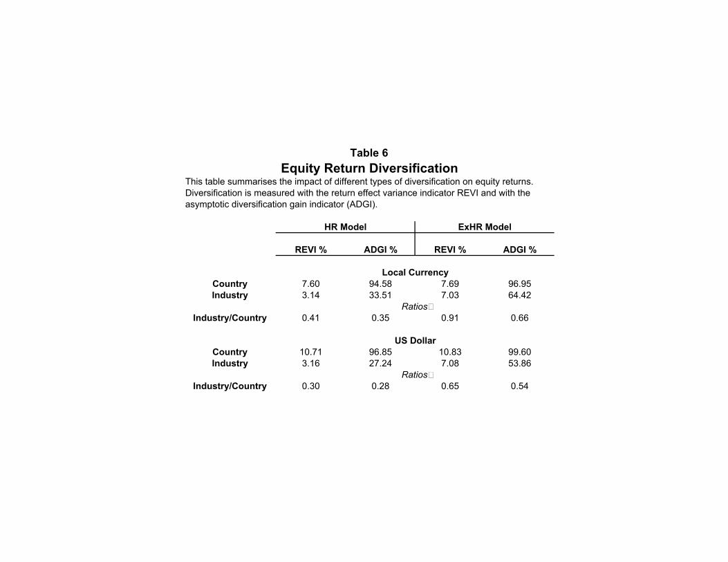
Table 6 Equity Return Diversification

This table summarises the impact of different types of diversification on equity returns. Diversification is measured with the return effect variance indicator REVI and with the asymptotic diversification gain indicator (ADGI).

HR Model ExHR Model

REVI % ADGI % REVI % ADGI %

Local Currency Country 7.60 94.58 7.69 96.95 Industry 3.14 33.51 7.03 64.42

Ratios Industry/Country 0.41 0.35 0.91 0.66

US Dollar Country 10.71 96.85 10.83 99.60 Industry 3.16 27.24 7.08 53.86

Ratios Industry/Country 0.30 0.28 0.65 0.54

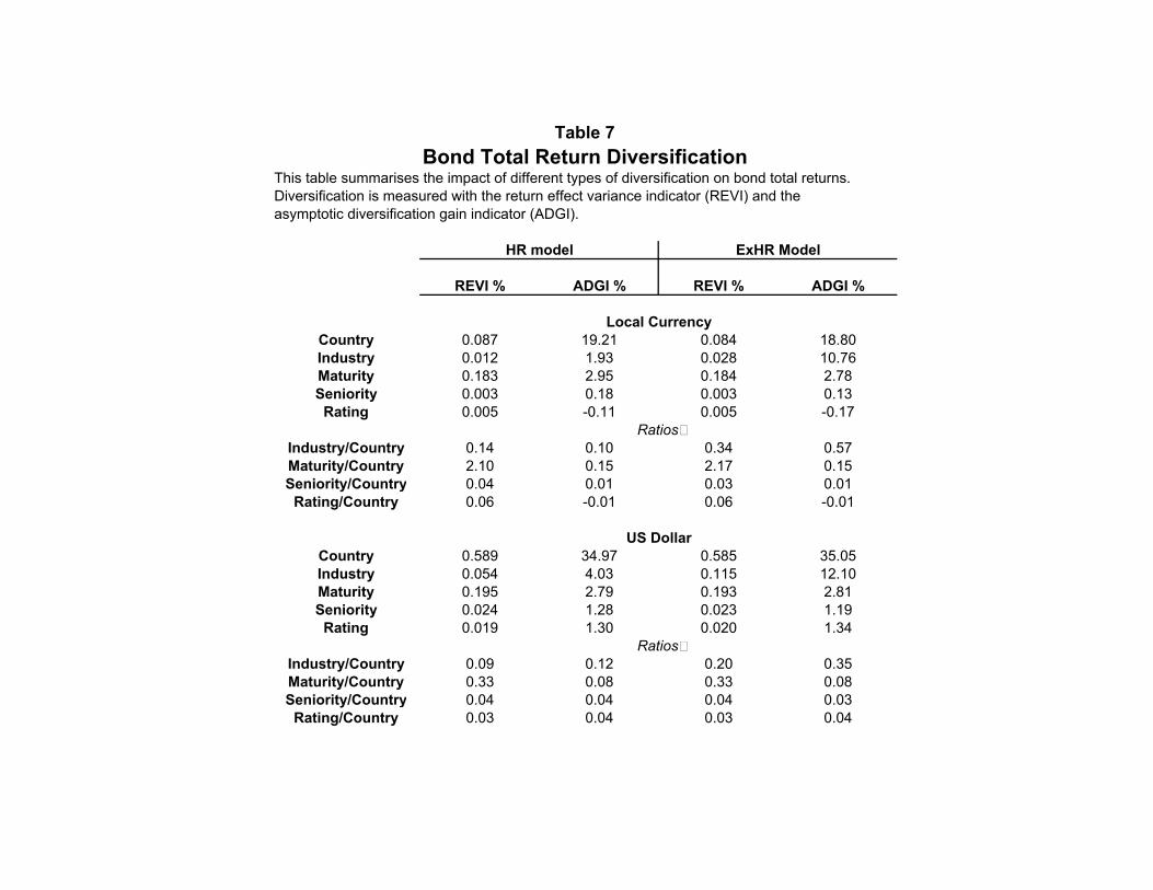
Table 7 Bond Total Return Diversification

This table summarises the impact of different types of diversification on bond total returns. Diversification is measured with the return effect variance indicator (REVI) and the asymptotic diversification gain indicator (ADGI).

HR model ExHR Model

REVI % ADGI % REVI % ADGI %

Local Currency Country 0.087 19.21 0.084 18.80 Industry 0.012 1.93 0.028 10.76 Maturity 0.183 2.95 0.184 2.78 Seniority 0.003 0.18 0.003 0.13

Rating 0.005 -0.11 0.005 -0.17 Ratios

Industry/Country 0.14 0.10 0.34 0.57 Maturity/Country 2.10 0.15 2.17 0.15 Seniority/Country 0.04 0.01 0.03 0.01

Rating/Country 0.06 -0.01 0.06 -0.01

US Dollar Country 0.589 34.97 0.585 35.05 Industry 0.054 4.03 0.115 12.10 Maturity 0.195 2.79 0.193 2.81 Seniority 0.024 1.28 0.023 1.19

Rating 0.019 1.30 0.020 1.34 Ratios

Industry/Country 0.09 0.12 0.20 0.35 Maturity/Country 0.33 0.08 0.33 0.08 Seniority/Country 0.04 0.04 0.04 0.03

Rating/Country 0.03 0.04 0.03 0.04

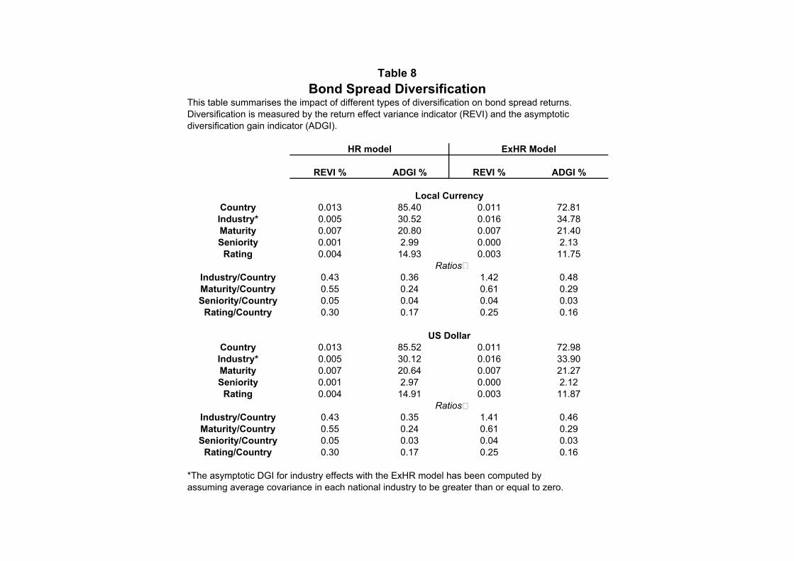
Table 8 Bond Spread Diversification

This table summarises the impact of different types of diversification on bond spread returns. Diversification is measured by the return effect variance indicator (REVI) and the asymptotic diversification gain indicator (ADGI).

HR model ExHR Model

REVI % ADGI % REVI % ADGI %

Local Currency Country 0.013 85.40 0.011 72.81 Industry* 0.005 30.52 0.016 34.78 Maturity 0.007 20.80 0.007 21.40 Seniority 0.001 2.99 0.000 2.13

Rating 0.004 14.93 0.003 11.75 Ratios

Industry/Country 0.43 0.36 1.42 0.48 Maturity/Country 0.55 0.24 0.61 0.29 Seniority/Country 0.05 0.04 0.04 0.03

Rating/Country 0.30 0.17 0.25 0.16

US Dollar Country 0.013 85.52 0.011 72.98 Industry* 0.005 30.12 0.016 33.90 Maturity 0.007 20.64 0.007 21.27 Seniority 0.001 2.97 0.000 2.12

Rating 0.004 14.91 0.003 11.87 Ratios

Industry/Country 0.43 0.35 1.41 0.46 Maturity/Country 0.55 0.24 0.61 0.29 Seniority/Country 0.05 0.03 0.04 0.03

Rating/Country 0.30 0.17 0.25 0.16

*The asymptotic DGI for industry effects with the ExHR model has been computed by assuming average covariance in each national industry to be greater than or equal to zero.