LUND UNIVERSITY

PO Box 117221 00 Lund+46 46-222 00 00

The Jitter Margin and Its Application in the Design of Real-Time Control Systems

Cervin, Anton; Lincoln, Bo; Eker, Johan; Årzén, Karl-Erik; Buttazzo, Giorgio

Published in:Proceedings of the 10th International Conference on Real-Time and Embedded Computing Systems andApplications

2004

Link to publication

Citation for published version (APA):Cervin, A., Lincoln, B., Eker, J., Årzén, K-E., & Buttazzo, G. (2004). The Jitter Margin and Its Application in theDesign of Real-Time Control Systems. In Proceedings of the 10th International Conference on Real-Time andEmbedded Computing Systems and Applications

General rightsCopyright and moral rights for the publications made accessible in the public portal are retained by the authorsand/or other copyright owners and it is a condition of accessing publications that users recognise and abide by thelegal requirements associated with these rights.

• Users may download and print one copy of any publication from the public portal for the purpose of private studyor research. • You may not further distribute the material or use it for any profit-making activity or commercial gain • You may freely distribute the URL identifying the publication in the public portalTake down policyIf you believe that this document breaches copyright please contact us providing details, and we will removeaccess to the work immediately and investigate your claim.

Download date: 23. Feb. 2019

10th International Conference on Real-Time and Embedded Computing Systems and Applications (RTCSA), Göteborg, Sweden, August 2004.

The Jitter Margin and Its Application in the Design of Real-TimeControl Systems

Anton Cervin,1 Bo Lincoln,2 Johan Eker,3 Karl-Erik Årzén, 4 Giorgio Buttazzo1

1Department of Computer Engineering and Systems Science, University of Pavia, Italy2 Glaze AB, Limhamn, Sweden

3 Ericsson Mobile Platforms AB, Lund, Sweden4 Department of Automatic Control, Lund Institute of Technology, Sweden

anton@control.lth.se

Abstract

Based on recent advances in control theory, we proposethe notion of jitter margin for periodic control tasks. Thejitter margin is defined as a function of the amount ofconstant delay in the control loop, and it describes howmuch additional time-varying delay can be tolerated beforethe loop goes unstable. Combined with scheduling theory,the jitter margin can be used to guarantee the stabilityand performance of the controller in the target system.It can also be used as a tool for assigning meaningfuldeadlines to control tasks. We discuss the need for best-caseresponse-time analysis in this context, and propose a simplelower bound under EDF scheduling. Finally, a control-scheduling codesign procedure is given, where periods areassigned iteratively to yield the same relative performancedegradation for each control task.

1. Introduction

1.1 Background and Motivation

In classical feedback control theory (e.g., [Franklin et al.,2002]), notions such as phase margin and gain margin areused to describe how sensitive a control loop is towards var-ious uncertainties in the plant. Nonnegative margins are re-quired to ensure the stability of the closed-loop system. Themargins are also used as practical stability measures, andthere are various rules of thumb associated with them. Forinstance, it is typically recommended to have a phase mar-gin of at least 30◦–45◦ to ensure some degree of robustnessand performance of the system.When a controller is implemented as a task in a real-time system, a new kind of uncertainty is introduced—animplementation uncertainty. In this paper, we will focuson the specific problem of output jitter. Variability in thetask execution time and preemption from other tasks cancause the controller to experience a different amount ofinput-output delay in each period. It is well known that

such a jitter can degrade the control performance and inextreme cases even cause instability of the control loop(e.g., [Törngren, 1998]). Although the present paper onlyconsiders jitter due to CPU scheduling, some of the resultsalso carry over to networked control systems, where jitterdue to variable transmission times is a major issue.The majority of previous work on jitter in real-time controlsystems has focused on either scheduling theory or controltheory. In the few instances where an integrated approachhas been taken, the control analysis has been somewhat un-derdeveloped. By contrast, our analysis yields hard resultsand should hence be applicable to a wide range of systems,including safety-critical applications.

1.2 Contributions

Recently, a new stability theorem for control loops withtime-varying input-output delays has been developed [Kaoand Lincoln, 2004]. Based on this theorem, we proposethe notion of jitter margin for control tasks. The jittermargin can be combined with real-time scheduling theoryto guarantee the stability and performance of the controllerin the target system. The jitter margin can also be used as atool for assigning meaningful deadlines to control tasks.It is noted that the jitter analysis can be improved ifbest-case response times, as well as worst-case responsetimes, can be computed. For this purpose, we propose alower bound on the best-case response time under EDFscheduling, where no such results are known to exist.When designing a real-time control system, informationabout the task timing is needed in the control design, andinformation about the controller timing sensitivity is neededin the real-time design. Based on this insight, we propose aniterative control–scheduling codesign procedure, where thejitter margin is used as a central tool.

1.3 Outline

This paper is outlined as follows. In Section 2, the assump-tions are given, and the jitter margin is defined. Its proper-

1

replacementsP(s)

K(z) ShZOH

∆

Σ−

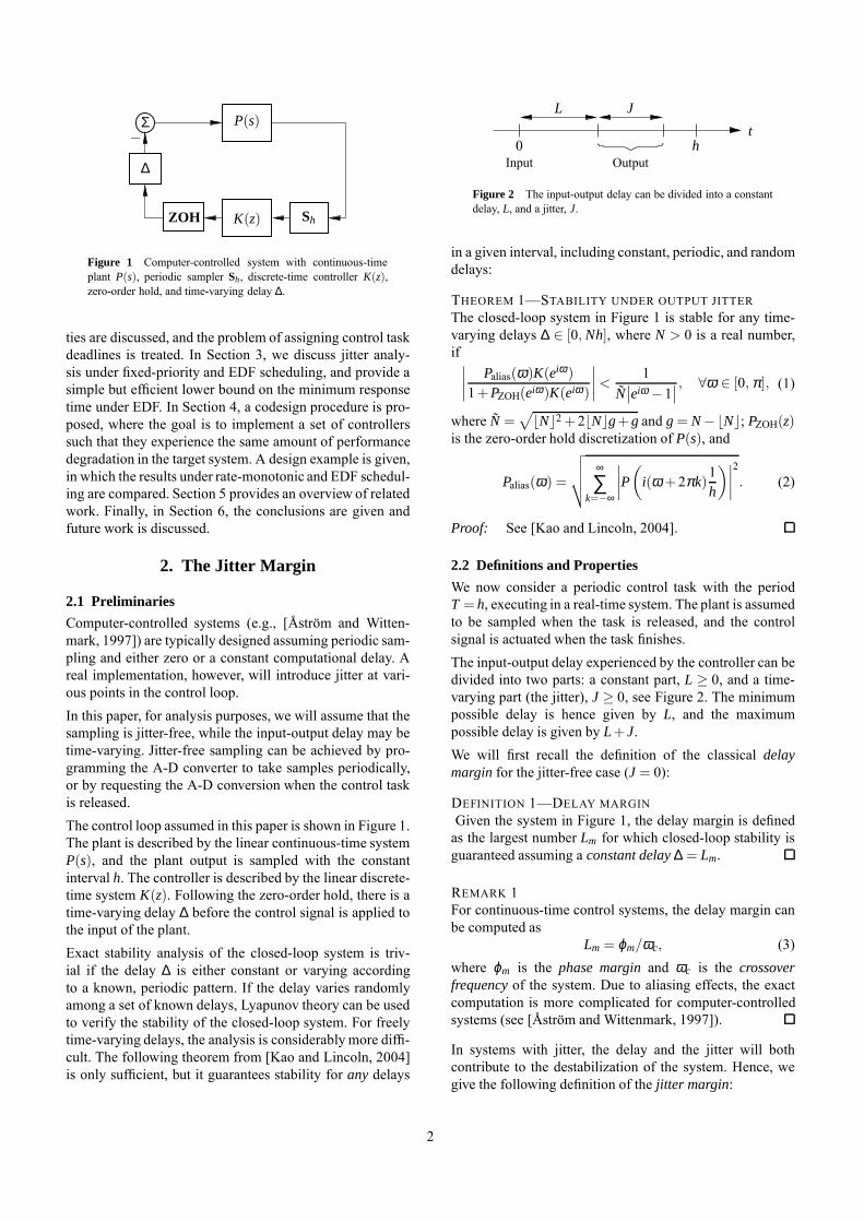
Figure 1 Computer-controlled system with continuous-timeplant P(s), periodic sampler Sh, discrete-time controller K(z),zero-order hold, and time-varying delay ∆.

ties are discussed, and the problem of assigning control taskdeadlines is treated. In Section 3, we discuss jitter analy-sis under fixed-priority and EDF scheduling, and provide asimple but efficient lower bound on the minimum responsetime under EDF. In Section 4, a codesign procedure is pro-posed, where the goal is to implement a set of controllerssuch that they experience the same amount of performancedegradation in the target system. A design example is given,in which the results under rate-monotonic and EDF schedul-ing are compared. Section 5 provides an overview of relatedwork. Finally, in Section 6, the conclusions are given andfuture work is discussed.

2. The Jitter Margin

2.1 Preliminaries

Computer-controlled systems (e.g., [Åström and Witten-mark, 1997]) are typically designed assuming periodic sam-pling and either zero or a constant computational delay. Areal implementation, however, will introduce jitter at vari-ous points in the control loop.In this paper, for analysis purposes, we will assume that thesampling is jitter-free, while the input-output delay may betime-varying. Jitter-free sampling can be achieved by pro-gramming the A-D converter to take samples periodically,or by requesting the A-D conversion when the control taskis released.The control loop assumed in this paper is shown in Figure 1.The plant is described by the linear continuous-time systemP(s), and the plant output is sampled with the constantinterval h. The controller is described by the linear discrete-time system K(z). Following the zero-order hold, there is atime-varying delay ∆ before the control signal is applied tothe input of the plant.Exact stability analysis of the closed-loop system is triv-ial if the delay ∆ is either constant or varying accordingto a known, periodic pattern. If the delay varies randomlyamong a set of known delays, Lyapunov theory can be usedto verify the stability of the closed-loop system. For freelytime-varying delays, the analysis is considerably more diffi-cult. The following theorem from [Kao and Lincoln, 2004]is only sufficient, but it guarantees stability for any delays

Input Output0

th

JL

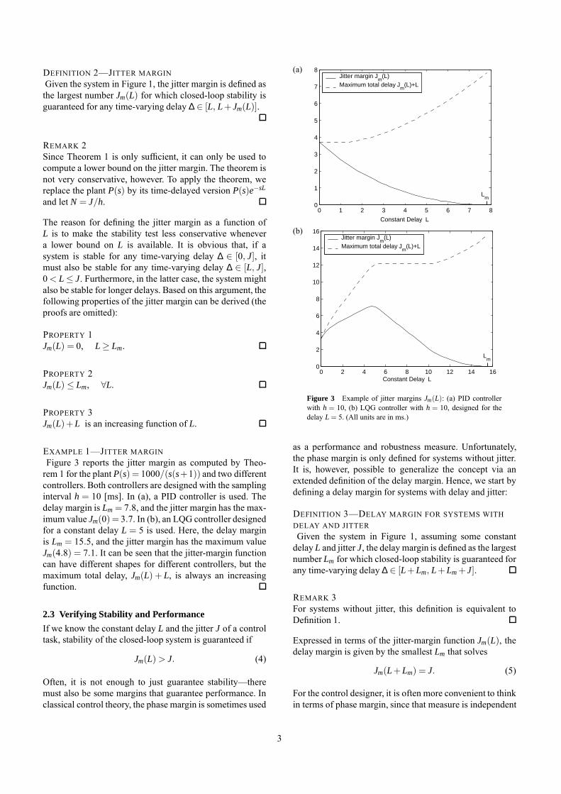
Figure 2 The input-output delay can be divided into a constantdelay, L, and a jitter, J.

in a given interval, including constant, periodic, and randomdelays:

THEOREM 1—STABILITY UNDER OUTPUT JITTERThe closed-loop system in Figure 1 is stable for any time-varying delays ∆ ∈ [0, Nh], where N > 0 is a real number,if

∣

∣

∣

∣

Palias(ω)K(eiω )

1+ PZOH(eiω)K(eiω )

∣

∣

∣

∣

<1

N∣

∣eiω −1∣

∣

, ∀ω ∈ [0, π ], (1)

where N =√

bNc2 +2bNcg + g and g = N −bNc; PZOH(z)is the zero-order hold discretization of P(s), and

Palias(ω) =

√

√

√

√

∞

∑k=−∞

∣

∣

∣

∣

P

(

i(ω +2πk)1h

)∣

∣

∣

∣

2. (2)

Proof: See [Kao and Lincoln, 2004].

2.2 Definitions and Properties

We now consider a periodic control task with the periodT = h, executing in a real-time system. The plant is assumedto be sampled when the task is released, and the controlsignal is actuated when the task finishes.The input-output delay experienced by the controller can bedivided into two parts: a constant part, L ≥ 0, and a time-varying part (the jitter), J ≥ 0, see Figure 2. The minimumpossible delay is hence given by L, and the maximumpossible delay is given by L+ J.We will first recall the definition of the classical delaymargin for the jitter-free case (J = 0):

DEFINITION 1—DELAY MARGINGiven the system in Figure 1, the delay margin is definedas the largest number Lm for which closed-loop stability isguaranteed assuming a constant delay ∆ = Lm.

REMARK 1For continuous-time control systems, the delay margin canbe computed as

Lm = ϕm/ωc, (3)where ϕm is the phase margin and ωc is the crossoverfrequency of the system. Due to aliasing effects, the exactcomputation is more complicated for computer-controlledsystems (see [Åström and Wittenmark, 1997]).

In systems with jitter, the delay and the jitter will bothcontribute to the destabilization of the system. Hence, wegive the following definition of the jitter margin:

2

DEFINITION 2—JITTER MARGINGiven the system in Figure 1, the jitter margin is defined asthe largest number Jm(L) for which closed-loop stability isguaranteed for any time-varying delay ∆ ∈ [L, L+ Jm(L)].

REMARK 2Since Theorem 1 is only sufficient, it can only be used tocompute a lower bound on the jitter margin. The theorem isnot very conservative, however. To apply the theorem, wereplace the plant P(s) by its time-delayed version P(s)e−sL

and let N = J/h.

The reason for defining the jitter margin as a function ofL is to make the stability test less conservative whenevera lower bound on L is available. It is obvious that, if asystem is stable for any time-varying delay ∆ ∈ [0, J], itmust also be stable for any time-varying delay ∆ ∈ [L, J],0< L ≤ J. Furthermore, in the latter case, the system mightalso be stable for longer delays. Based on this argument, thefollowing properties of the jitter margin can be derived (theproofs are omitted):

PROPERTY 1Jm(L) = 0, L ≥ Lm.

PROPERTY 2Jm(L) ≤ Lm, ∀L.

PROPERTY 3Jm(L)+ L is an increasing function of L.

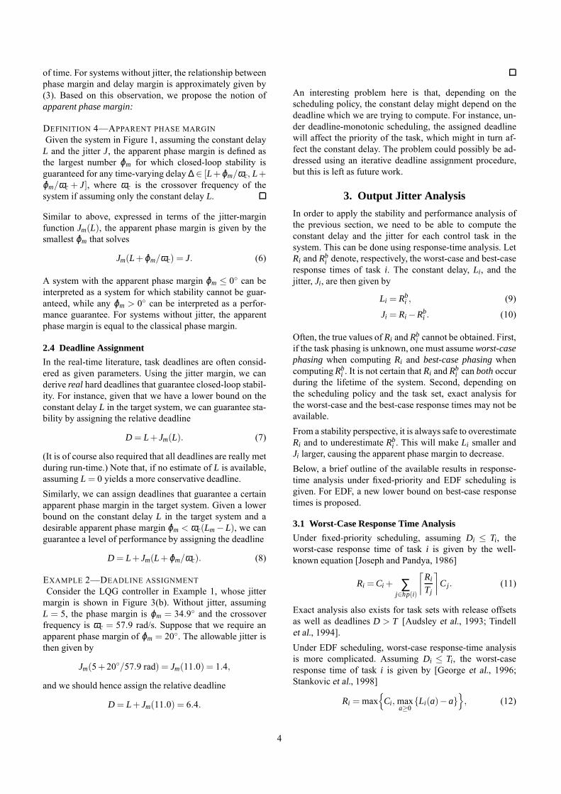
EXAMPLE 1—JITTER MARGINFigure 3 reports the jitter margin as computed by Theo-rem 1 for the plant P(s) = 1000/(s(s+1)) and two differentcontrollers. Both controllers are designed with the samplinginterval h = 10 [ms]. In (a), a PID controller is used. Thedelay margin is Lm = 7.8, and the jitter margin has the max-imum value Jm(0) = 3.7. In (b), an LQG controller designedfor a constant delay L = 5 is used. Here, the delay marginis Lm = 15.5, and the jitter margin has the maximum valueJm(4.8) = 7.1. It can be seen that the jitter-margin functioncan have different shapes for different controllers, but themaximum total delay, Jm(L) + L, is always an increasingfunction.

2.3 Verifying Stability and Performance

If we know the constant delay L and the jitter J of a controltask, stability of the closed-loop system is guaranteed if

Jm(L) > J. (4)

Often, it is not enough to just guarantee stability—theremust also be some margins that guarantee performance. Inclassical control theory, the phase margin is sometimes used

(a)

0 1 2 3 4 5 6 7 80

1

2

3

4

5

6

7

8

Constant Delay L

Jitter margin Jm

(L)Maximum total delay J

m(L)+L

Lm

(b)

0 2 4 6 8 10 12 14 160

2

4

6

8

10

12

14

16

Constant Delay L

Jitter margin Jm

(L)Maximum total delay J

m(L)+L

Lm

Figure 3 Example of jitter margins Jm(L): (a) PID controllerwith h = 10, (b) LQG controller with h = 10, designed for thedelay L = 5. (All units are in ms.)

as a performance and robustness measure. Unfortunately,the phase margin is only defined for systems without jitter.It is, however, possible to generalize the concept via anextended definition of the delay margin. Hence, we start bydefining a delay margin for systems with delay and jitter:

DEFINITION 3—DELAY MARGIN FOR SYSTEMS WITHDELAY AND JITTERGiven the system in Figure 1, assuming some constantdelay L and jitter J, the delay margin is defined as the largestnumber Lm for which closed-loop stability is guaranteed forany time-varying delay ∆ ∈ [L+ Lm, L+ Lm + J].

REMARK 3For systems without jitter, this definition is equivalent toDefinition 1.

Expressed in terms of the jitter-margin function Jm(L), thedelay margin is given by the smallest Lm that solves

Jm(L+ Lm) = J. (5)

For the control designer, it is often more convenient to thinkin terms of phase margin, since that measure is independent

3

of time. For systems without jitter, the relationship betweenphase margin and delay margin is approximately given by(3). Based on this observation, we propose the notion ofapparent phase margin:

DEFINITION 4—APPARENT PHASE MARGINGiven the system in Figure 1, assuming the constant delay

L and the jitter J, the apparent phase margin is defined asthe largest number ϕm for which closed-loop stability isguaranteed for any time-varying delay ∆ ∈ [L+ ϕm/ωc, L+ϕm/ωc + J], where ωc is the crossover frequency of thesystem if assuming only the constant delay L.

Similar to above, expressed in terms of the jitter-marginfunction Jm(L), the apparent phase margin is given by thesmallest ϕm that solves

Jm(L+ ϕm/ωc) = J. (6)

A system with the apparent phase margin ϕm ≤ 0◦ can beinterpreted as a system for which stability cannot be guar-anteed, while any ϕm > 0◦ can be interpreted as a perfor-mance guarantee. For systems without jitter, the apparentphase margin is equal to the classical phase margin.

2.4 Deadline Assignment

In the real-time literature, task deadlines are often consid-ered as given parameters. Using the jitter margin, we canderive real hard deadlines that guarantee closed-loop stabil-ity. For instance, given that we have a lower bound on theconstant delay L in the target system, we can guarantee sta-bility by assigning the relative deadline

D = L+ Jm(L). (7)

(It is of course also required that all deadlines are really metduring run-time.) Note that, if no estimate of L is available,assuming L = 0 yields a more conservative deadline.Similarly, we can assign deadlines that guarantee a certainapparent phase margin in the target system. Given a lowerbound on the constant delay L in the target system and adesirable apparent phase margin ϕm < ωc(Lm −L), we canguarantee a level of performance by assigning the deadline

D = L+ Jm(L+ ϕm/ωc). (8)

EXAMPLE 2—DEADLINE ASSIGNMENTConsider the LQG controller in Example 1, whose jittermargin is shown in Figure 3(b). Without jitter, assumingL = 5, the phase margin is ϕm = 34.9◦ and the crossoverfrequency is ωc = 57.9 rad/s. Suppose that we require anapparent phase margin of ϕm = 20◦. The allowable jitter isthen given by

Jm(5+20◦/57.9 rad) = Jm(11.0) = 1.4,

and we should hence assign the relative deadline

D = L+ Jm(11.0) = 6.4.

An interesting problem here is that, depending on thescheduling policy, the constant delay might depend on thedeadline which we are trying to compute. For instance, un-der deadline-monotonic scheduling, the assigned deadlinewill affect the priority of the task, which might in turn af-fect the constant delay. The problem could possibly be ad-dressed using an iterative deadline assignment procedure,but this is left as future work.

3. Output Jitter Analysis

In order to apply the stability and performance analysis ofthe previous section, we need to be able to compute theconstant delay and the jitter for each control task in thesystem. This can be done using response-time analysis. LetRi and Rb

i denote, respectively, the worst-case and best-caseresponse times of task i. The constant delay, Li, and thejitter, Ji, are then given by

Li = Rbi , (9)

Ji = Ri −Rbi . (10)

Often, the true values of Ri and Rbi cannot be obtained. First,

if the task phasing is unknown, one must assume worst-casephasing when computing Ri and best-case phasing whencomputing Rb

i . It is not certain that Ri and Rbi can both occur

during the lifetime of the system. Second, depending onthe scheduling policy and the task set, exact analysis forthe worst-case and the best-case response times may not beavailable.From a stability perspective, it is always safe to overestimateRi and to underestimate Rb

i . This will make Li smaller andJi larger, causing the apparent phase margin to decrease.Below, a brief outline of the available results in response-time analysis under fixed-priority and EDF scheduling isgiven. For EDF, a new lower bound on best-case responsetimes is proposed.

3.1 Worst-Case Response Time Analysis

Under fixed-priority scheduling, assuming Di ≤ Ti, theworst-case response time of task i is given by the well-known equation [Joseph and Pandya, 1986]

Ri = Ci + ∑j∈hp(i)

⌈

Ri

Tj

⌉

C j. (11)

Exact analysis also exists for task sets with release offsetsas well as deadlines D > T [Audsley et al., 1993; Tindellet al., 1994].Under EDF scheduling, worst-case response-time analysisis more complicated. Assuming Di ≤ Ti, the worst-caseresponse time of task i is given by [George et al., 1996;Stankovic et al., 1998]

Ri =max{

Ci, maxa≥0

{Li(a)−a}}

, (12)

4

where the busy interval Li(a) is given by the equation

Li(a) = Wi(

a,Li(a))

+

(

1+

⌊

aTi

⌋)

Ci, (13)

and the higher-priority workloadWi(a,t) is given by

Wi(a,t) = ∑j 6=i,D j≤a+Di

min{⌈

tTj

⌉

, 1+

⌊

a + Di−D j

Tj

⌋}

C j.

(14)It should be noted that only a finite number of values ofa must be checked when evaluating (12). The analysis hasalso been generalized to arbitrary deadlines [George et al.,1996].

3.2 Best-Case Response Time Analysis

Under fixed-priority scheduling, exact best-case analysishas recently been developed for the case D ≤ T [Redell andSanfridson, 2002]. The best-case response time of task i isgiven by the equation

Rbi = Cb

i + ∑j∈hp(i)

⌈

Rbi

Tj−1

⌉

Cbj , (15)

whereCbi denotes the best-case execution time of task i.

Under EDF scheduling, no exact best-case analysis isknown to exist. A trivial lower bound Ri on the best-caseresponse time of task i is given by

Rbi = Cb

i . (16)

This is actually a quite good bound for the shortest-periodtasks. The longest-period tasks can, however, have muchlonger best-case response times, especially if the systemload is high.A tighter lower bound on the best-case response time canbe obtained by interference analysis, see Appendix A. Ourproposed lower bound, Ri, is given by the equation

Rbi = Cb

i + ∑∀ j:D j<Rb

i

⌈

min{

Rbi , Di −D j

}

Tj−1

⌉

Cbj , (17)

which can be solved by recursion from above (cf. [Redelland Sanfridson, 2002]).The results obtained with the proposed bound have beencompared to results obtained by simulation, where theshortest response time of each task was recorded. (Notethat the latter constitutes an upper bound on the real best-case response time.) The bounds were evaluated for loadsranging from U = 0.5 to U = 0.99. For each load case,100 random task sets were generated. The number of tasksin each set was integer-uniformly distributed between 2and 10. The task periods were exponentially distributedwith mean 1, and the fraction of the execution time to theperiod was uniformly distributed between 0 and 1. Theexecution times were uniformly rescaled to give the task

0.5 0.6 0.7 0.8 0.9 1

1

1.5

2

2.5

U

mea

n(R

b n/Cn)

Upper bound (from simulation)Proposed lower boundTrivial lower bound

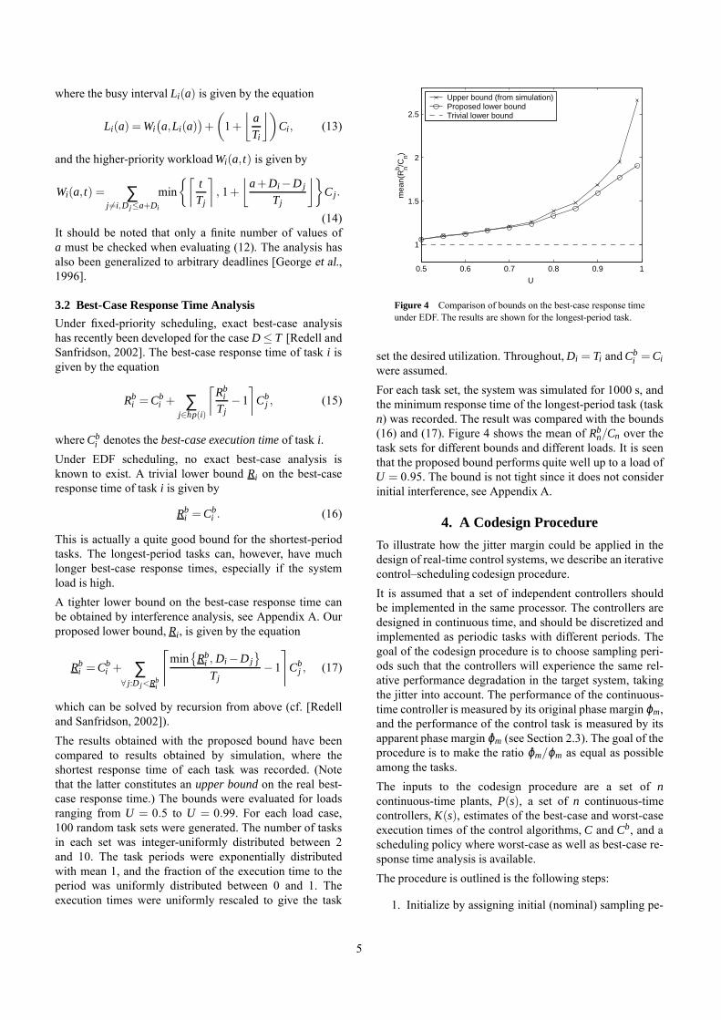
Figure 4 Comparison of bounds on the best-case response timeunder EDF. The results are shown for the longest-period task.

set the desired utilization. Throughout,Di = Ti andCbi = Ci

were assumed.For each task set, the system was simulated for 1000 s, andthe minimum response time of the longest-period task (taskn) was recorded. The result was compared with the bounds(16) and (17). Figure 4 shows the mean of Rb

n/Cn over thetask sets for different bounds and different loads. It is seenthat the proposed bound performs quite well up to a load ofU = 0.95. The bound is not tight since it does not considerinitial interference, see Appendix A.

4. A Codesign Procedure

To illustrate how the jitter margin could be applied in thedesign of real-time control systems, we describe an iterativecontrol–scheduling codesign procedure.It is assumed that a set of independent controllers shouldbe implemented in the same processor. The controllers aredesigned in continuous time, and should be discretized andimplemented as periodic tasks with different periods. Thegoal of the codesign procedure is to choose sampling peri-ods such that the controllers will experience the same rel-ative performance degradation in the target system, takingthe jitter into account. The performance of the continuous-time controller is measured by its original phase margin ϕm,and the performance of the control task is measured by itsapparent phase margin ϕm (see Section 2.3). The goal of theprocedure is to make the ratio ϕm/ϕm as equal as possibleamong the tasks.The inputs to the codesign procedure are a set of ncontinuous-time plants, P(s), a set of n continuous-timecontrollers, K(s), estimates of the best-case and worst-caseexecution times of the control algorithms, C and Cb, and ascheduling policy where worst-case as well as best-case re-sponse time analysis is available.The procedure is outlined is the following steps:

1. Initialize by assigning initial (nominal) sampling pe-

5

riods h for the controllers. (A common rule of thumb[Åström andWittenmark, 1997] is to choose the sam-pling period such that ωbh ∈ [0.2, 0.6], where ωb isthe bandwidth of the closed-loop continuous system.)

2. Rescale the periods linearly such that the task set be-comes schedulable under the given scheduling policy.(Here, a suitable sufficient schedulability test can beused.)

3. Discretize the controllers using the assigned samplingperiods, yielding the set of discrete-time controllersK(z).

4. For each task, compute worst-case and best-caseresponse times, R and Rb. (Here, the analysis inSection 3 is applicable.)

5. For each task, compute the jitter margin using Theo-rem 1 and the apparent phase margin ϕmi from (6),assuming the constant delay Li = Rb

i and the jitterJi = Ri −Rb

i .

6. For each task, compute the relative performancedegradation ri = ϕmi/ϕmi. Also, compute their meanvalue, r = ∑ ri/n.

7. For each task, adjust the period according to

hi := hi + khi(ri − r)/r,

where k < 1 is a gain parameter.

8. Repeat from 2 until no further improvement is given.A suitable stop criterion is when sum of the perfor-mance differences, ∑ |ri − r|, is no longer decreasing.

The period adjustment mechanism in step 7 is intended todecrease the periods of controllers with bad performance,and to increase the periods of controllers with good per-formance. Choosing the gain parameter can be difficult. Asmall k will give slow adaptation, while a large k can causeinstability.The iterative procedure tries to solve a highly nonlin-ear optimization problem. Hence, it is not certain that itwill converge to an optimal solution. For instance, underrate-monotonic scheduling, a small period adjustment maychange the task priorities, and this can in turn have a hugeimpact on the jitter. Neither is it certain that a completelyequal performance degradation can be achieved.

EXAMPLE 3—CODESIGNWe consider an example where three controllers shouldbe implemented in a single CPU. Both rate-monotonic andEDF scheduling is considered. The execution times of thecontrol algorithms are assumed to be equal and constant andare given by R = Rb = 0.15 [ms]. The plants to be controlled

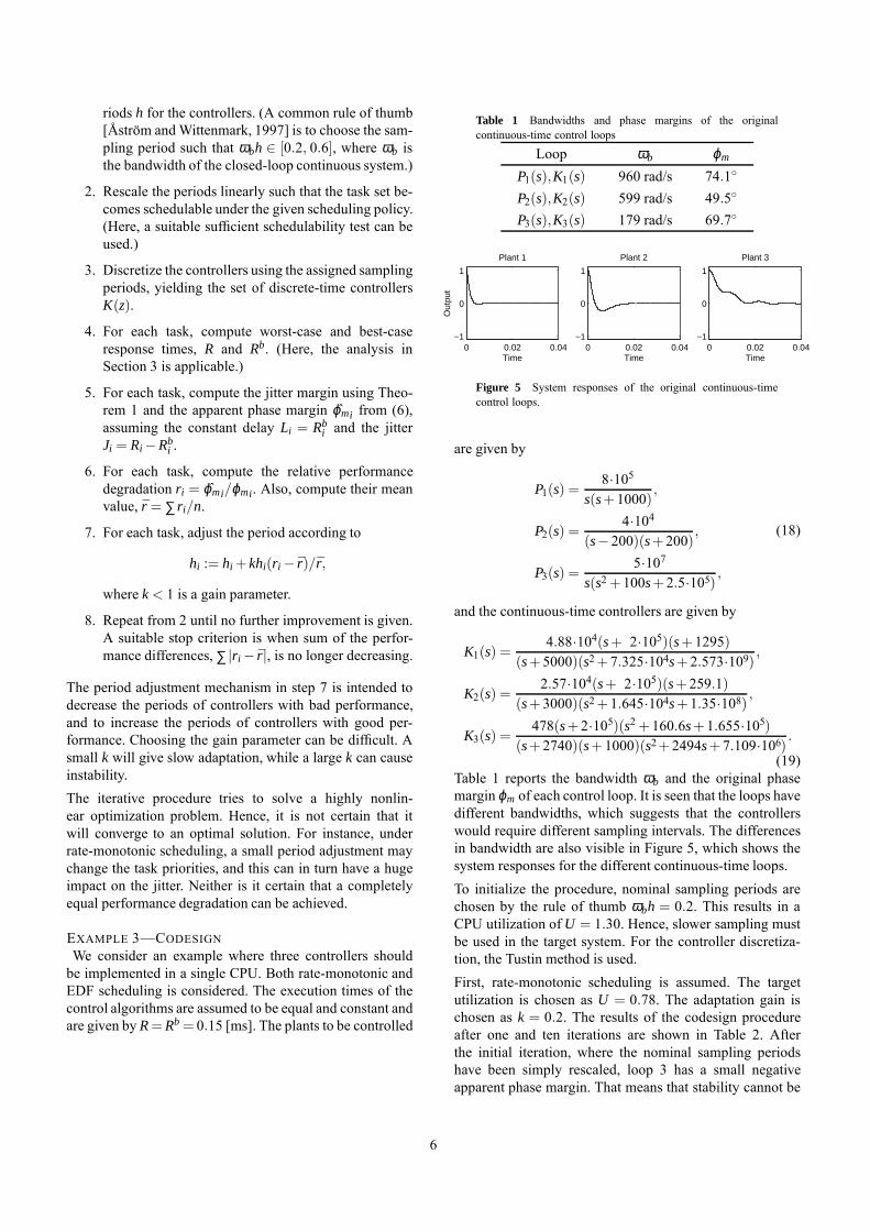
Table 1 Bandwidths and phase margins of the originalcontinuous-time control loops

Loop ωb ϕm

P1(s),K1(s) 960 rad/s 74.1◦

P2(s),K2(s) 599 rad/s 49.5◦

P3(s),K3(s) 179 rad/s 69.7◦

0 0.02 0.04−1

0

1

Time

Out

put

Plant 1

0 0.02 0.04−1

0

1

Time

Plant 2

0 0.02 0.04−1

0

1

Time

Plant 3

Figure 5 System responses of the original continuous-timecontrol loops.

are given by

P1(s) =8·105

s(s+1000),

P2(s) =4·104

(s−200)(s+200),

P3(s) =5·107

s(s2 +100s+2.5·105),

(18)

and the continuous-time controllers are given by

K1(s) =4.88·104(s+ 2·105)(s+1295)

(s+5000)(s2+7.325·104s+2.573·109),

K2(s) =2.57·104(s+ 2·105)(s+259.1)

(s+3000)(s2+1.645·104s+1.35·108),

K3(s) =478(s+2·105)(s2 +160.6s+1.655·105)

(s+2740)(s+1000)(s2+2494s+7.109·106).

(19)Table 1 reports the bandwidth ωb and the original phasemarginϕm of each control loop. It is seen that the loops havedifferent bandwidths, which suggests that the controllerswould require different sampling intervals. The differencesin bandwidth are also visible in Figure 5, which shows thesystem responses for the different continuous-time loops.To initialize the procedure, nominal sampling periods arechosen by the rule of thumb ωbh = 0.2. This results in aCPU utilization of U = 1.30. Hence, slower sampling mustbe used in the target system. For the controller discretiza-tion, the Tustin method is used.First, rate-monotonic scheduling is assumed. The targetutilization is chosen as U = 0.78. The adaptation gain ischosen as k = 0.2. The results of the codesign procedureafter one and ten iterations are shown in Table 2. Afterthe initial iteration, where the nominal sampling periodshave been simply rescaled, loop 3 has a small negativeapparent phase margin. That means that stability cannot be

6

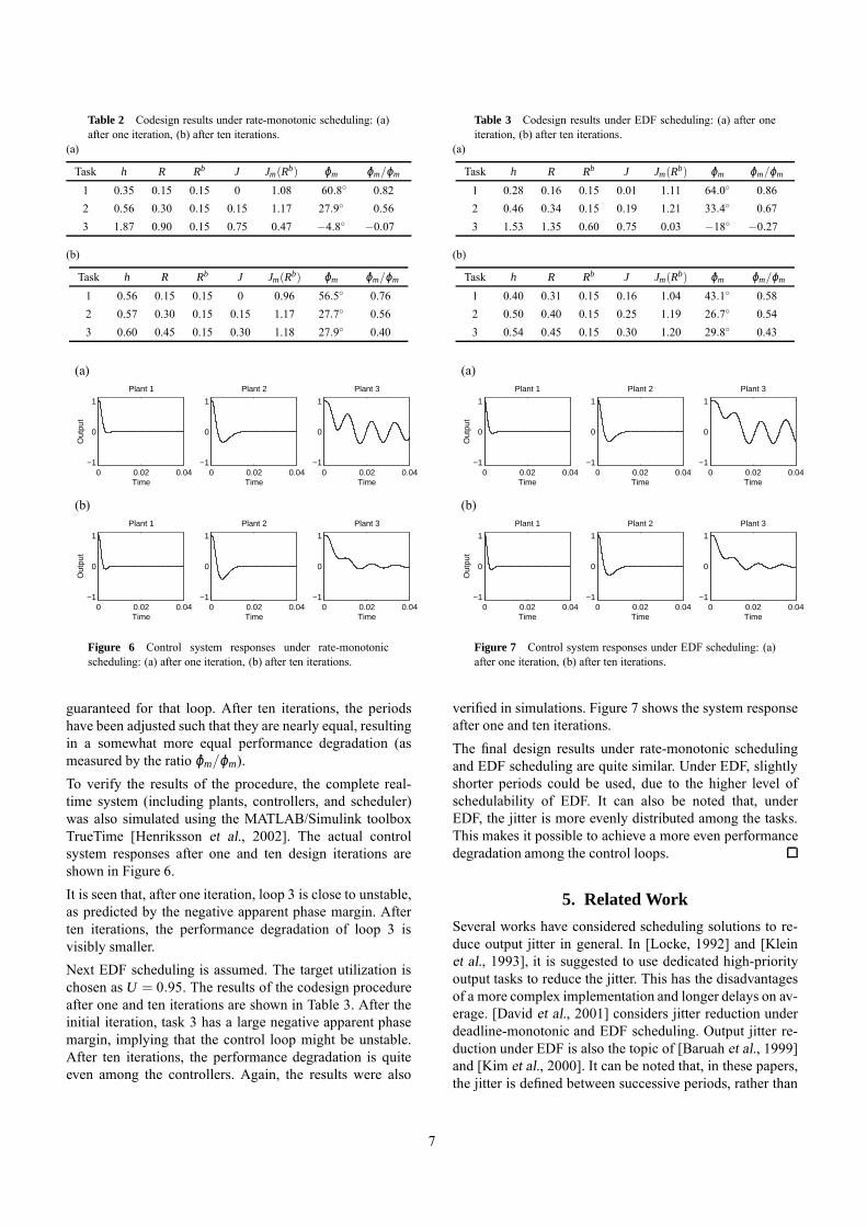
Table 2 Codesign results under rate-monotonic scheduling: (a)after one iteration, (b) after ten iterations.

(a)

Task h R Rb J Jm(Rb) ϕm ϕm/ϕm

1 0.35 0.15 0.15 0 1.08 60.8◦ 0.822 0.56 0.30 0.15 0.15 1.17 27.9◦ 0.563 1.87 0.90 0.15 0.75 0.47 −4.8◦ −0.07

(b)

Task h R Rb J Jm(Rb) ϕm ϕm/ϕm

1 0.56 0.15 0.15 0 0.96 56.5◦ 0.762 0.57 0.30 0.15 0.15 1.17 27.7◦ 0.563 0.60 0.45 0.15 0.30 1.18 27.9◦ 0.40

(a)

0 0.02 0.04−1

0

1

Time

Out

put

Plant 1

0 0.02 0.04−1

0

1

Time

Plant 2

0 0.02 0.04−1

0

1

Time

Plant 3

(b)

0 0.02 0.04−1

0

1

Time

Out

put

Plant 1

0 0.02 0.04−1

0

1

Time

Plant 2

0 0.02 0.04−1

0

1

Time

Plant 3

Figure 6 Control system responses under rate-monotonicscheduling: (a) after one iteration, (b) after ten iterations.

guaranteed for that loop. After ten iterations, the periodshave been adjusted such that they are nearly equal, resultingin a somewhat more equal performance degradation (asmeasured by the ratio ϕm/ϕm).To verify the results of the procedure, the complete real-time system (including plants, controllers, and scheduler)was also simulated using the MATLAB/Simulink toolboxTrueTime [Henriksson et al., 2002]. The actual controlsystem responses after one and ten design iterations areshown in Figure 6.It is seen that, after one iteration, loop 3 is close to unstable,as predicted by the negative apparent phase margin. Afterten iterations, the performance degradation of loop 3 isvisibly smaller.Next EDF scheduling is assumed. The target utilization ischosen as U = 0.95. The results of the codesign procedureafter one and ten iterations are shown in Table 3. After theinitial iteration, task 3 has a large negative apparent phasemargin, implying that the control loop might be unstable.After ten iterations, the performance degradation is quiteeven among the controllers. Again, the results were also

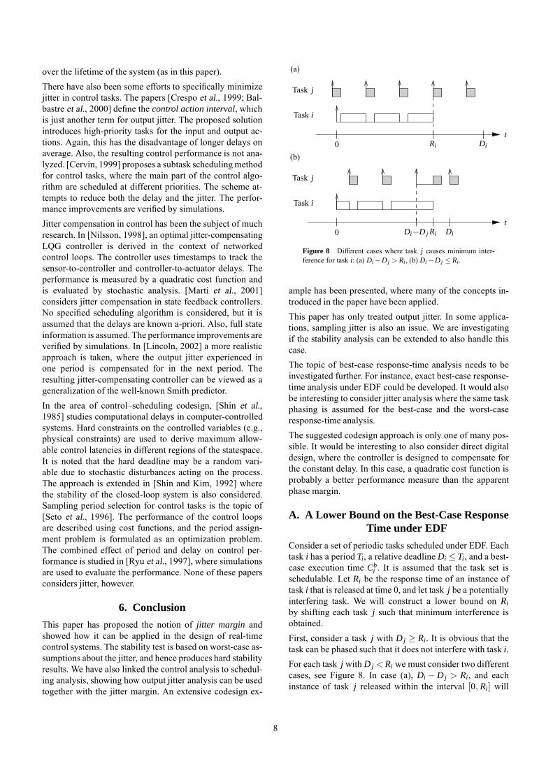
Table 3 Codesign results under EDF scheduling: (a) after oneiteration, (b) after ten iterations.

(a)

Task h R Rb J Jm(Rb) ϕm ϕm/ϕm

1 0.28 0.16 0.15 0.01 1.11 64.0◦ 0.862 0.46 0.34 0.15 0.19 1.21 33.4◦ 0.673 1.53 1.35 0.60 0.75 0.03 −18◦ −0.27

(b)

Task h R Rb J Jm(Rb) ϕm ϕm/ϕm

1 0.40 0.31 0.15 0.16 1.04 43.1◦ 0.582 0.50 0.40 0.15 0.25 1.19 26.7◦ 0.543 0.54 0.45 0.15 0.30 1.20 29.8◦ 0.43

(a)

0 0.02 0.04−1

0

1

Time

Out

put

Plant 1

0 0.02 0.04−1

0

1

Time

Plant 2

0 0.02 0.04−1

0

1

Time

Plant 3

(b)

0 0.02 0.04−1

0

1

Time

Out

put

Plant 1

0 0.02 0.04−1

0

1

Time

Plant 2

0 0.02 0.04−1

0

1

Time

Plant 3

Figure 7 Control system responses under EDF scheduling: (a)after one iteration, (b) after ten iterations.

verified in simulations. Figure 7 shows the system responseafter one and ten iterations.The final design results under rate-monotonic schedulingand EDF scheduling are quite similar. Under EDF, slightlyshorter periods could be used, due to the higher level ofschedulability of EDF. It can also be noted that, underEDF, the jitter is more evenly distributed among the tasks.This makes it possible to achieve a more even performancedegradation among the control loops.

5. Related Work

Several works have considered scheduling solutions to re-duce output jitter in general. In [Locke, 1992] and [Kleinet al., 1993], it is suggested to use dedicated high-priorityoutput tasks to reduce the jitter. This has the disadvantagesof a more complex implementation and longer delays on av-erage. [David et al., 2001] considers jitter reduction underdeadline-monotonic and EDF scheduling. Output jitter re-duction under EDF is also the topic of [Baruah et al., 1999]and [Kim et al., 2000]. It can be noted that, in these papers,the jitter is defined between successive periods, rather than

7

over the lifetime of the system (as in this paper).There have also been some efforts to specifically minimizejitter in control tasks. The papers [Crespo et al., 1999; Bal-bastre et al., 2000] define the control action interval, whichis just another term for output jitter. The proposed solutionintroduces high-priority tasks for the input and output ac-tions. Again, this has the disadvantage of longer delays onaverage. Also, the resulting control performance is not ana-lyzed. [Cervin, 1999] proposes a subtask schedulingmethodfor control tasks, where the main part of the control algo-rithm are scheduled at different priorities. The scheme at-tempts to reduce both the delay and the jitter. The perfor-mance improvements are verified by simulations.Jitter compensation in control has been the subject of muchresearch. In [Nilsson, 1998], an optimal jitter-compensatingLQG controller is derived in the context of networkedcontrol loops. The controller uses timestamps to track thesensor-to-controller and controller-to-actuator delays. Theperformance is measured by a quadratic cost function andis evaluated by stochastic analysis. [Marti et al., 2001]considers jitter compensation in state feedback controllers.No specified scheduling algorithm is considered, but it isassumed that the delays are known a-priori. Also, full stateinformation is assumed. The performance improvements areverified by simulations. In [Lincoln, 2002] a more realisticapproach is taken, where the output jitter experienced inone period is compensated for in the next period. Theresulting jitter-compensating controller can be viewed as ageneralization of the well-known Smith predictor.In the area of control–scheduling codesign, [Shin et al.,1985] studies computational delays in computer-controlledsystems. Hard constraints on the controlled variables (e.g.,physical constraints) are used to derive maximum allow-able control latencies in different regions of the statespace.It is noted that the hard deadline may be a random vari-able due to stochastic disturbances acting on the process.The approach is extended in [Shin and Kim, 1992] wherethe stability of the closed-loop system is also considered.Sampling period selection for control tasks is the topic of[Seto et al., 1996]. The performance of the control loopsare described using cost functions, and the period assign-ment problem is formulated as an optimization problem.The combined effect of period and delay on control per-formance is studied in [Ryu et al., 1997], where simulationsare used to evaluate the performance. None of these papersconsiders jitter, however.

6. Conclusion

This paper has proposed the notion of jitter margin andshowed how it can be applied in the design of real-timecontrol systems. The stability test is based on worst-case as-sumptions about the jitter, and hence produces hard stabilityresults. We have also linked the control analysis to schedul-ing analysis, showing how output jitter analysis can be usedtogether with the jitter margin. An extensive codesign ex-

(a)

(b)

Task j

Task j

Task i

Task i

0

0

t

t

Ri

Ri

Di

Di

Di−D j

Figure 8 Different cases where task j causes minimum inter-ference for task i: (a) Di −D j > Ri, (b) Di −D j ≤ Ri.

ample has been presented, where many of the concepts in-troduced in the paper have been applied.This paper has only treated output jitter. In some applica-tions, sampling jitter is also an issue. We are investigatingif the stability analysis can be extended to also handle thiscase.The topic of best-case response-time analysis needs to beinvestigated further. For instance, exact best-case response-time analysis under EDF could be developed. It would alsobe interesting to consider jitter analysis where the same taskphasing is assumed for the best-case and the worst-caseresponse-time analysis.The suggested codesign approach is only one of many pos-sible. It would be interesting to also consider direct digitaldesign, where the controller is designed to compensate forthe constant delay. In this case, a quadratic cost function isprobably a better performance measure than the apparentphase margin.

A. A Lower Bound on the Best-Case ResponseTime under EDF

Consider a set of periodic tasks scheduled under EDF. Eachtask i has a period Ti, a relative deadline Di ≤ Ti, and a best-case execution time Cb

i . It is assumed that the task set isschedulable. Let Ri be the response time of an instance oftask i that is released at time 0, and let task j be a potentiallyinterfering task. We will construct a lower bound on Ri

by shifting each task j such that minimum interference isobtained.First, consider a task j with D j ≥ Ri. It is obvious that thetask can be phased such that it does not interfere with task i.For each task j with D j < Ri we must consider two differentcases, see Figure 8. In case (a), Di − D j > Ri, and eachinstance of task j released within the interval [0, Ri] will

8

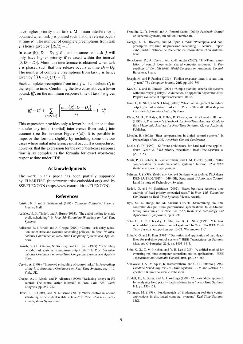
have higher priority than task i. Minimum interference isobtained when task j is phased such that one release occursat time Ri. The number of complete preemptions from taskj is hence given by dRi/Tj −1e.In case (b), Di − D j ≤ Ri, and instances of task j willonly have higher priority if released within the interval[0, Di −D j]. Minimum interference is obtained when taskj is phased such that one release occurs at time Di −D j.The number of complete preemptions from task j is hencegiven by d(Di −D j)/Tj −1e.Each complete preemption from task j will contributeC j tothe response time. Combining the two cases above, a lowerbound, Rb

i , on the minimum response time of task i is givenby

Rbi = Cb

i + ∑∀ j:D j<Rb

i

⌈

min{

Rbi , Di −D j

}

Tj−1

⌉

Cbj

This expression provides only a lower bound, since it doesnot take any initial (partial) interference from task j intoaccount (see for instance Figure 8(a)). It is possible toimprove the formula slightly by including some obviouscases where initial interferencemust occur. It is conjectured,however, that the expression for the exact best-case responsetime is as complex as the formula for exact worst-caseresponse time under EDF.

Acknowledgments

The work in this paper has been partially supportedby EU/ARTIST (http://www.artist-embedded.org) and bySSF/FLEXCON (http://www.control.lth.se/FLEXCON).

ReferencesÅström, K. J. and B. Wittenmark (1997): Computer-Controlled Systems.

Prentice Hall.

Audsley, N., K. Tindell, and A. Burns (1993): “The end of the line for staticcyclic scheduling.” In Proc. 5th Euromicro Workshop on Real-TimeSystems.

Balbastre, P., I. Ripoll, and A. Crespo (2000): “Control task delay reduc-tion under static and dynamic scheduling policies.” In Proc. 7th Inter-national Conference on Real-Time Computing Systems and Applica-tions.

Baruah, S., G. Buttazzo, S. Gorinsky, and G. Lipari (1999): “Schedulingperiodic task systems to minimize output jitter.” In Proc. 6th Inter-national Conference on Real-Time Computing Systems and Applica-tions.

Cervin, A. (1999): “Improved scheduling of control tasks.” In Proceedingsof the 11th Euromicro Conference on Real-Time Systems, pp. 4–10.York, UK.

Crespo, A., I. Ripoll, and P. Albertos (1999): “Reducing delays in RTcontrol: The control action interval.” In Proc. 14th IFAC WorldCongress, pp. 257–262.

David, L., F. Cottet, and N. Nissanke (2001): “Jitter control in on-linescheduling of dependent real-time tasks.” In Proc. 22nd IEEE Real-Time Systems Symposium.

Franklin, G., D. Powell, and A. Emami-Naeini (2002): Feedback Controlof Dynamic Systems, 4th edition. Prentice Hall.

George, L., N. Rivierre, and M. Spuri (1996): “Preemptive and non-preemptive real-time uniprocessor scheduling.” Technical Report2966. Institut National de Recherche en Informatique et en Automa-tique.

Henriksson, D., A. Cervin, and K.-E. Årzén (2002): “TrueTime: Simu-lation of control loops under shared computer resources.” In Pro-ceedings of the 15th IFAC World Congress on Automatic Control.Barcelona, Spain.

Joseph, M. and P. Pandya (1986): “Finding response times in a real-timesystem.” The Computer Journal, 29:5, pp. 390–395.

Kao, C.-Y. and B. Lincoln (2004): “Simple stability criteria for systemswith time-varying delays.” Automatica. To appear in September 2004.Preprint available at http://www.control.lth.se.

Kim, T., H. Shin, and N. Chang (2000): “Deadline assignment to reduceoutput jitter of real-time tasks.” In Proc. 16th IFAC Workshop onDistributed Computer Control Systems.

Klein, M. H., T. Ralya, B. Pollak, R. Obenza, and M. Gonzalez Härbour(1993): A Practitioner’s Handbook for Real-Time Analysis: Guide toRate Monotonic Analysis for Real-Time Systems. Kluwer AcademicPublisher.

Lincoln, B. (2002): “Jitter compensation in digital control systems.” InProceedings of the 2002 American Control Conference.

Locke, C. D. (1992): “Software architecture for hard real-time applica-tions: Cyclic vs. fixed priority executives.” Real-Time Systems, 4,pp. 37–53.

Marti, P., G. Fohler, K. Ramamritham, and J. M. Fuertes (2001): “Jittercompensation for real-time control systems.” In Proc. 22nd IEEEReal-Time Systems Symposium.

Nilsson, J. (1998): Real-Time Control Systems with Delays. PhD thesisISRN LUTFD2/TFRT--1049--SE, Department of Automatic Control,Lund Institute of Technology, Sweden.

Redell, O. and M. Sanfridson (2002): “Exact best-case response timeanalysis of fixed priority scheduled tasks.” In Proc. 14th EuromicroConference on Real-Time Systems. Vienna, Austria.

Ryu, M., S. Hong, and M. Saksena (1997): “Streamlining real-timecontroller design: From performance specifications to end-to-endtiming constraints.” In Proc. 3rd IEEE Real-Time Technology andApplications Symposium, pp. 91–99.

Seto, D., J. P. Lehoczky, L. Sha, and K. G. Shin (1996): “On taskschedulability in real-time control systems.” In Proc. 17th IEEE Real-Time Systems Symposium, pp. 13–21. Washington, DC.

Shin, K. G. and H. Kim (1992): “Derivation and application of hard dead-lines for real-time control systems.” IEEE Transactions on Systems,Man, and Cybernetics, 22:6, pp. 1403–1413.

Shin, K. G., C. M. Krishna, and Y.-H. Lee (1985): “A unified method forevauating real-time computer controllers and its applications.” IEEETransactions on Automatic Control, 30:4, pp. 357–366.

Stankovic, J. A., M. Spuri, K. Ramamritham, and G. C. Buttazzo (1998):Deadline Scheduling for Real-Time Systems—EDF and Related Al-gorithms. Kluwer Academic Publishers.

Tindell, K., A. Burns, and A. J. Wellings (1994): “An extendible approachfor analyzing fixed priority hard real-time tasks.” Real-Time Systems,6:2, pp. 133–151.

Törngren, M. (1998): “Fundamentals of implementing real-time controlapplications in distributed computer systems.” Real-Time Systems,14:3.

9