The Italian block of the ESCB multi-country model Elena Angelini, Antonello D‘Agostino ISSN 1561081-0 9 771561 081005 WORKING PAPER SERIES NO 660 / JULY 2006 THE ITALIAN BLOCK OF

ISSN 1561081-0

9 7 7 1 5 6 1 0 8 1 0 0 5

WORKING PAPER SER IESNO 660 / JULY 2006

THE ITALIAN BLOCK OF THE ESCB MULTI-COUNTRY MODEL

by Elena Angelini,Antonello D‘Agostinoand Peter McAdam

In 2006 all ECB publications will feature

a motif taken from the

€5 banknote.

WORK ING PAPER SER IE SNO 660 / JULY 2006

This paper can be downloaded without charge from http://www.ecb.int or from the Social Science Research Network

electronic library at http://ssrn.com/abstract_id=913335

1 We are grateful to many colleagues in the Econometric Modelling Division of the Directorate General Research of the ECB, and from the Working Group on Econometric Modelling for discussions and comments, in particular Frederic Boissay, Tohmas Karlsson, Alberto

Locarno and Alpo Willman. The views expressed here are not necessarily those of the ECB or of the Eurosystem. This paper was written when Antonello D‘Agostino was working in the Research Department of the European Central Bank.

3 Central Bank and Financial Services Authority of Ireland, P.O. Box 559/Dame Street, Dublin 2, Ireland; e-mail: [email protected]

4 European Central Bank, Kaiserstrasse 29, 60311 Frankfurt am Main, Germany; e-mail: [email protected]

THE ITALIAN BLOCK OF THE ESCB

MULTI-COUNTRY MODEL 1

by Elena Angelini 2,Antonello D‘Agostino 3

and Peter McAdam 4

2 European Central Bank, Kaiserstrasse 29, 60311 Frankfurt am Main, Germany; e-mail: [email protected]

© European Central Bank, 2006

AddressKaiserstrasse 2960311 Frankfurt am Main, Germany

Postal addressPostfach 16 03 1960066 Frankfurt am Main, Germany

Telephone+49 69 1344 0

Internethttp://www.ecb.int

Fax+49 69 1344 6000

Telex411 144 ecb d

All rights reserved.

Any reproduction, publication andreprint in the form of a differentpublication, whether printed orproduced electronically, in whole or inpart, is permitted only with the explicitwritten authorisation of the ECB or theauthor(s).

The views expressed in this paper do notnecessarily reflect those of the EuropeanCentral Bank.

The statement of purpose for the ECBWorking Paper Series is available fromthe ECB website, http://www.ecb.int.

ISSN 1561-0810 (print)ISSN 1725-2806 (online)

3ECB

Working Paper Series No 660July 2006

CONTENTS

Abstract 4Non-technical summary 5

1 Introduction 6

2 The theoretical background of theItalian MCM: the supply side 7

2.1 7

2.2 The firm’s programme 7

2.3 Phillips curve and NAIRU 8

2.4 Calibration of the supply side parameters 10

2.5 Solving the model 10

2.6 The demand side and output components 12

3 The estimated equations 13

3.1 The supply side 13

3.2 Short run dynamics 14

3.3 Demand components (consumption,investment, trade) and prices 20

4 The steady state and simulation propertiesof the Italian MCM 33

4.1 Policy rules 33

4.2 Steady state 34

4.3 Illustrative simulations 35

5 Conclusions 52

References 52

6 Appendix A: Names of variables in theItalian MCM 54

7 Appendix B: List of dummies and trends

European Central Bank Working Paper Series 67

An overview

56

Abstract

This paper documents the structure, estimation and simulation properties ofthe Italian block of the ESCB-multi-country model (MCM). The model is usedregularly as an input into Eurosystem projection exercises and, to a lesser extent,in simulation analysis. The specification of the Italian model follows closely thatof the Area-Wide Model (AWM) and indeed the other MCM country blocks (interms of specification and accounting framework). The MCM is a quarterly es-timated structural macroeconomic model that treats the economy in a relativelyclosed manner. It has a long-run classical equilibrium with a vertical Phillips curvebut with some short-run frictions in price/wage setting and factor demands. Con-sequently, activity is demand-determined in the short-run but supply-determinedin the longer run with employment having converged to a level consistent with anexogenously given level of equilibrium unemployment. The precise properties ofthe model are illustrated using a number of standard variant simulations.

JEL Classification: C3, C5, E1, E2

Keywords: Macro-econometric Modelling, Italy

4ECBWorking Paper Series No 660July 2006

Non-technical Summary

This paper documents the structure, estimation and simulation properties of theItalian block of the ESCB-multi-country model (MCM). This model is regularly usedas an input into Eurosystem projection exercises and, to a lesser extent, in simulationanalysis. The specification of the model follows closely that of the Area-Wide Model(AWM) and indeed the other MCM country blocks (in terms of specification and ac-counting framework). Specifically, the MCM is a quarterly estimated macroeconomicmodel that treats the economy as essentially closed. It has a long-run classical equi-librium with a vertical Phillips curve but with some short-run frictions in price/wagesetting and factor demands. Consequently, activity is demand-determined in the short-run but supply-determined in the longer run with employment having converged toa level consistent with the exogenously given level of equilibrium unemployment. Toillustrate the precise properties of the model, we include a formal presentation of itstheoretical and econometric underpinnings and analyse the effects of five exogenouspermanent shocks to the economy.

5ECB


1 Introduction

This paper documents the structure, estimation and simulation properties of the Ital-ian block of the ESCB-multi-country model (MCM). This model is used regularly asan input into Eurosystem projection exercises and, to a lesser extent, in simulationanalysis. The specification of the Italian model follows closely (in terms of specificationand accounting framework) that of the Area-Wide Model (AWM) and indeed the otherMCM country blocks (e.g., Willman and Estrada, 2002; Boissay and Villetelle, 2005;Angelini, Boissay, and Ciccarelli, 2006).1 Consequently, and necessarily, this paperclosely follows the exposition of other MCMs published so far.

The Italian MCM is a quarterly estimated macroeconomic model that treats theeconomy in a relatively closed nature. It has a long-run classical equilibrium with a ver-tical Phillips curve but with some short-run frictions in price/wage setting and factordemands. Consequently, activity is demand-determined in the short-run but supply-determined in the longer run with employment having converged to a level consistentwith the exogenously given level of equilibrium unemployment. Stock-flow adjustmentsare accounted for by, for example, the inclusion of a wealth term in consumption. Atpresent, the treatment of expectations in the model is limited given that the modelembodies backward-looking expectations. The model has a total of 126 equations, ofwhich 18 are estimated behavioural equations; the rest are identities, quasi-identitiesand policy rules. Production in the economy is modelled as a single aggregate sector,with demand being the sum of components: private and public consumption, invest-ment, stock-building and net trade. As regards the nominal side, there is quite a richstructure of (pre- and post-tax) prices with the GDP deflator modelled as a (fixed)mark-up over production costs. This deflator is essentially the foundation for all otherprices in the models. The (nominal) exchange rate is exogenous, whereas the (nominal)interest rate may follow a Taylor-type rule.

Although the Italian MCM belongs firmly in the AWM/MCM class of models,some points of departure (of various importance) are worth mentioning. First, andmost obviously, the Italian MCM is estimated on its own national database and thusit will embody particular point estimates and polynomial lengths in equations and,thus, different response times and dynamic behaviour, relative to other MCM countryblocks. Second, in the Italian model, dynamic homogeneity is only imposed wherethere is supporting statistical evidence; given that imposing dynamic homogeneity canrender a model excessively cyclical. Third, our modelling of the supply side was donein terms of pre-tax concepts; thus for example in our wage equation the productivity /NAIRU nexus is derived under factor cost prices rather market prices to maintain thatunemployment is independent of taxes, similarly, the long-run level of potential outputis independent of taxes.

The paper proceeds as follows. Section 2 presents an overview of the main featuresof the model and the theoretical specification, followed by a detailed equation ’by’equation presentation in section 3. Section 4 assesses the dynamic properties of themodel through a set of standard variant simulations, and section 5 concludes.

1Karlsson and McAdam (2005) give an overview of the MCM framework and the (trade) Link block.


2 The Theoretical Background of the Italian MCM: TheSupply Side

2.1 An Overview

The structure of the Italian MCM is relatively standard, built on an aggregate de-mand/aggregate supply framework, with a well-defined long-run classical supply-sideequilibrium, and a vertical long-run Phillips curve, with an exogenous natural rate(NAIRU). The steady-state real interest rate pins down the capital-to-output ratioof the unemployment rate, via the firm’s marginal productivity optimality condition.Since the labour force is given in the long-run, steady-state output is then equal to theproduction-function outcome with a zero NAIRU gap. In that equilibrium, all real vari-ables grow at the same rate as potential output, real wages grow in line with long-runlabour productivity, and relative prices are constant, in particular the real exchangerate. The model also takes into account stock-flow consistency, so that for examplehouseholds’ wealth (comprising total capital stock, public debt and net foreign assets)is also determined in GDP points at the steady state. With the steady-state publicdebt ratio pinned down by a fiscal rule and the steady-state capital stock determinedby the marginal productivity condition, this relation determines the steady-state ratioof net foreign assets to GDP.2

In the short-run, since variables do not immediately adjust to their steady-statevalues, the model has some Keynesian features, whereby output is constrained by thesum of demand components. The resulting departure from equilibrium in both thegoods and labour markets exerts influence on short-run price and wage developments,via an output gap and an unemployment gap term, respectively. The convergence tothe long run is ensured by the responses of policies to deviations from equilibrium.Fiscal policy is modelled as a change in direct tax rates responding to deviations froma target fiscal ratio to GDP and monetary policy is assumed to follow a Taylor-typerule, with a given nominal exchange rate.

2.2 The firm’s programme

Firms maximize profits for a given technology and level of demand3.The solution to the firms’ profit-maximization problem is given by individual prices

Pi, labour demand Li, capital demand Ki, and output Yi which depend on the aggregateproduction level Y , the general price level P , real wages w/P (w being the nominalwage) and the nominal cost of capital c. By definition:

c ≡ P (r + δ) (2.1)

where r is the real rate of interest and δ is the depreciation rate of capital. Assuming,no capital adjustment costs, this leads to,

2Typical long-run features and closures incorporated into macro models are discussed further inMcAdam (1999).

3Given the existing literature on the MCM framework, the subsequent sections closely follow thetreatment in Willman and Estrada (2002) and, more recently, Angelini, Boissay and Ciccarelli (2006)andBoissay and Villetelle (2005).

7ECB


maxLi,Ki

Π(Yi) = PiYi − wLi − cKi

s.t.

Pi = P(

YYi

)1/ε

Yi = AKβi

(eγtLi

)1−β

where ε > 1 is the elasticity of the demand for good i to its relative price and γis the (exogenous) growth rate of technological progress. The new capital goods arehomogenous to the consumption goods, and the price of new capital goods is P . Firmstake the nominal capital cost and nominal wages as given, since the latter depend onthe general level of price P .

maxLi,Ki

Π(Yi) = PY 1/εYε−1

εi − wLi − cKi

s.t.

Yi = AKβi

(eγtLi

)1−β

The solution to this programme is given by its first order conditions and, in thesymmetric equilibrium (where Pi = P , Yi = Y , Li = L and Ki = K ∀i), we obtain:

(a) : L = e−γt[

YAKβ

] 11−β

(b) : K = YAe(1−β)γt

[βw

(1−β)P (r+δ)

]1−β

(c) : wP = (1−β)(ε−1)

εYL

(2.2)

At this stage, given our assumption of constant returns to scale, the level of aggre-gate output is undetermined. These three relations determine the optimal capital tolabour ratio, labour productivity, and real wages. To determine the levels of output,employment and capital, one more condition has to be met on the labour market side.In a frictionless economy where real wages adjust to labour productivity, the level ofemployment would adjust to the (exogenous) labour force and full employment wouldprevail. In equilibrium, aggregate output and the stock of capital would be determinedby the level of the labour force. However, in an economy where firms and unions bar-gain on nominal wages, real wages may not be only driven by labour productivity, butalso by the rate of unemployment. In this situation, real wages are set above theirfrictionless equilibrium level and unemployment arises. The equilibrium rate of unem-ployment and the exogenous labour force then determine the level of employment, theaggregate output and the stock of capital.

2.3 Phillips curve and NAIRU

Nominal wages are indexed to the level of prices, but also depend on the unions’ bar-gaining power, which depends on the unemployment rate. This is modelled throughthe following general Phillips curve:

∆ log w = ∆ log P + φ (∆ log Y −∆log L) + ρ− η log (u) (2.3)


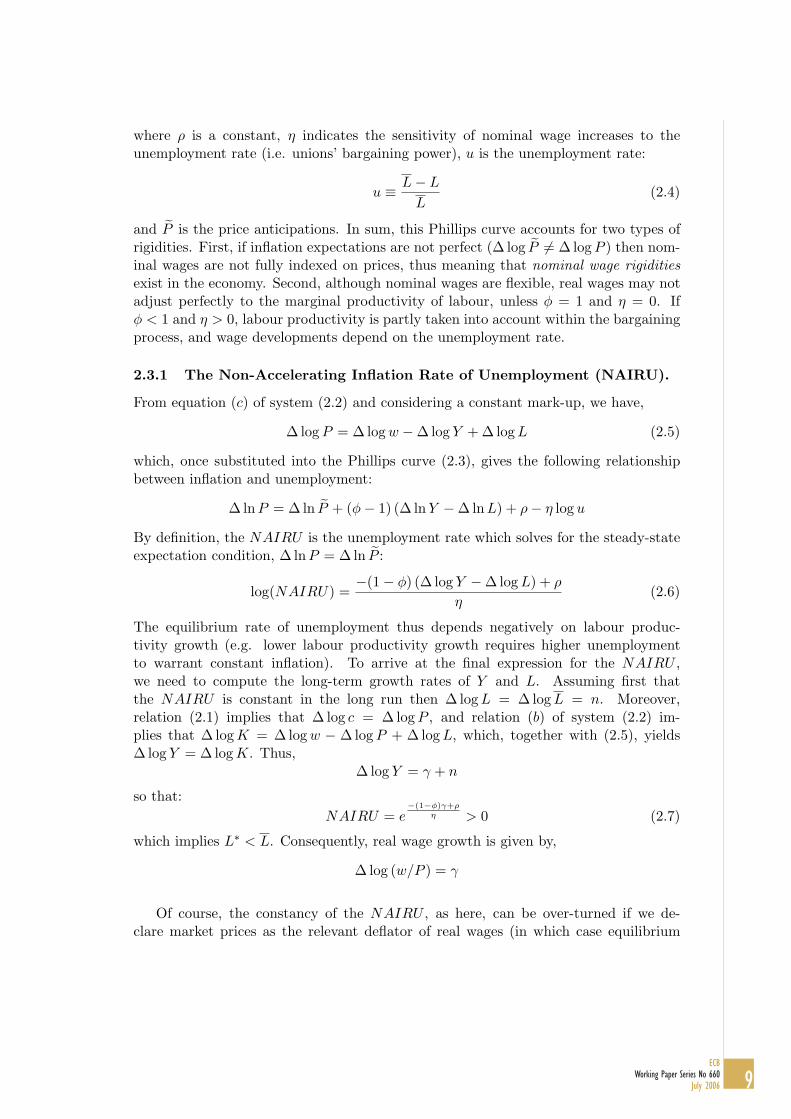
where ρ is a constant, η indicates the sensitivity of nominal wage increases to theunemployment rate (i.e. unions’ bargaining power), u is the unemployment rate:

u ≡ L− L

L(2.4)

and P is the price anticipations. In sum, this Phillips curve accounts for two types ofrigidities. First, if inflation expectations are not perfect (∆ log P 6= ∆ log P ) then nom-inal wages are not fully indexed on prices, thus meaning that nominal wage rigiditiesexist in the economy. Second, although nominal wages are flexible, real wages may notadjust perfectly to the marginal productivity of labour, unless φ = 1 and η = 0. Ifφ < 1 and η > 0, labour productivity is partly taken into account within the bargainingprocess, and wage developments depend on the unemployment rate.

2.3.1 The Non-Accelerating Inflation Rate of Unemployment (NAIRU).

From equation (c) of system (2.2) and considering a constant mark-up, we have,

∆ log P = ∆ log w −∆ log Y + ∆ log L (2.5)

which, once substituted into the Phillips curve (2.3), gives the following relationshipbetween inflation and unemployment:

∆ lnP = ∆ ln P + (φ− 1) (∆ lnY −∆ lnL) + ρ− η log u

By definition, the NAIRU is the unemployment rate which solves for the steady-stateexpectation condition, ∆ lnP = ∆ ln P :

log(NAIRU) =−(1− φ) (∆ log Y −∆log L) + ρ

η(2.6)

The equilibrium rate of unemployment thus depends negatively on labour produc-tivity growth (e.g. lower labour productivity growth requires higher unemploymentto warrant constant inflation). To arrive at the final expression for the NAIRU ,we need to compute the long-term growth rates of Y and L. Assuming first thatthe NAIRU is constant in the long run then ∆ log L = ∆ log L = n. Moreover,relation (2.1) implies that ∆ log c = ∆ log P , and relation (b) of system (2.2) im-plies that ∆ log K = ∆ log w − ∆log P + ∆ log L, which, together with (2.5), yields∆ log Y = ∆ log K. Thus,

∆ log Y = γ + n

so that:NAIRU = e

−(1−φ)γ+ρη > 0 (2.7)

which implies L∗ < L. Consequently, real wage growth is given by,

∆ log (w/P ) = γ

Of course, the constancy of the NAIRU , as here, can be over-turned if we de-clare market prices as the relevant deflator of real wages (in which case equilibrium

9ECB


unemployment is a function of average taxes, which in fact accords with typical unionbargaining models), or if the deflator used is the consumer price index (rather thansimply the domestic deflator), in which case, it the NAIRU would vary with the termsof trade.

2.4 Calibration of the Supply Side Parameters

The theoretical model as just described contains 5 parameters, β, ε, γ, A, and n,(i.e., the elasticity of output with respect to capital; the price elasticity of demand;the growth rate of exogenous labour productivity; technical level in the productionfunction; and the growth rate of the labour supply) and 5 real variables (Y , L, K, c/P ,w/P ). Denoting the sample mean operator by a bar above a variable, and using system(2.2), we calibrated these parameters as,

β =

((r + δ)K

wP L + (r + δ)K

); ε =

(PY

PY − wL− cK

); γ =

(∆log

(w

P

))

and

A =

Y

K β(eγtL

)1−β

;n =

(∆log(L)

)

2.5 Solving the model

The relations (2.3) and (2.4) close the model and enable the whole real side of thesteady state of the economy to be solved. These two relations determine the NAIRUand thereby the long-run level of labour. The latter being given, the solution of system(2.2) provides the steady state levels of Y , K, and w/P as functions of the parametersof the model and the real user cost of capital. The nominal variables of the model arenot determined by the supply side and do not affect the real economy in the long run.

2.5.1 Desired level of capital, long run real wages, and potential output.

The desired level of capital, denoted by K∗, corresponds to the level of the capital stockthat solves the maximization problem of the firm, for a given aggregate demand Y anda relative price of capital c/w (see equation (b) of system (2.2)):

K∗ =Y

Ae(1−β)γt

[βw

(1− β)P (r + δ)

]1−β

(2.8)

In the MCM, the long run targets appear in logarithms in the error correction term ofthe short run dynamic equations:

log(K∗) = log(Y ) + (1− β)

[log

(βw

(1− β)P (r + δ)

)− γt

]− log(A) (2.9)


Basically, K∗ depends on the (calibrated) elasticity of output to capital, β, and onlabour productivity growth, γ.4 The desired level of the capital stock is,

log(K∗) = log(Y ) + (1− β)

[log

(βw

(1− β)P (r + δ)

)− γt

](2.10)

using the standard law of motion for capital,

K = (1− δ)Kt−1 + I

we can derive long-run desired investment,

log(I∗) = log(

γ + n + δ

1 + γ + n

)+ log(K∗) (2.11)

where K∗ is defined by equation (2.10), so that I∗ also depends on the real cost ofcapital. Similarly, potential output and the target value of real wages are respectivelydrawn from relations (a) and (c) of system (2.2):

log(

w

P

∗)= log

((1− β)(ε− 1)

ε

)+ log

(Y

L

)(2.12)

log(Y ∗) = log(A) + β log(K) + (1− β) log(L) + (1− β)γt (2.13)

2.5.2 The desired level of labour.

As mentioned earlier, the Phillips curve is vertical in the long run. The long run unem-ployment rate, together with the exogenous labour force, determine the long run levelof labour: L∗∗ = (1−NAIRU)L. With a constant NAIRU and an exogenous labourforce, this specification will however generally not provide a relevant target for the dy-namics of actual employment. The reason is that the relevant information necessaryto model the labour force and labour participation in a satisfactory way is not avail-able in the MCM framework, where labour force is modelled as a simple autoregressiveprocess. In order to have a good fit of the short term dynamic employment equation,we will therefore not use L∗∗ in the definition of the error correction term. Instead,the common practice in the MCM framework is to define the latter as the differencebetween actual employment L and an ad hoc reference level L∗∗, which is derived fromthe production function (see equation (a) of system (2.2)):

log(L∗) =1

1− β

[log(Y )− β log(K)− log (A)

]− γt (2.14)

Since this definition is a re-writing of relation (2.13), the employment gap L − L∗

that we will use in the short run dynamic equation of labour is in fact a re-writing ofthe output gap Y −Y ∗ (see Section (2.3.1)). In the long run, the convergence process of

4Note, the gap between actual and desired variables may exhibit some drifts in-sample. To obtaina stationary gap, we have, where necessary, included constants and deterministic time trends over andabove those required in the estimation, these ensure that the error correction terms are mean stationary.

11ECB


the supply side to its steady state takes place as follows. First, actual employment willconverge toward the reference level L∗. Given equations (2.13) and (2.15), this ensures,by construction, that the output gap closes in the long run. Finally, employment adjuststo its long term level L∗∗ thanks to the Phillips curve, whose verticality in the long runwarrants that the unemployment rate converges toward the NAIRU and, therefore,that L converges toward L∗∗.

2.6 The Demand Side and Output Components

In order to allow a flexible econometric estimation of GDP components, the specificationof the demand side of the MCM is not formally derived explicitly from microeconomictheory.

2.6.1 Households’ Behaviour

The households sector only includes one behavioural equation for private consumption,which is a fairly standard specification. We do not, for example, consider housinginvestment separately. Private consumption (PCR) is a function of real disposableincome (PY R), comprising compensation, transfers of taxes and other income, and ofreal financial wealth (FWR), defined as cumulated savings under the assumption thathouseholds own all of the assets in the economy (i.e. public debt, net foreign assets,and private capital stock):5

log(PCR∗) = a + b log(PY R) + c log(FWR) + ε (2.15)

where a, b, c are coefficients and ε denotes all other factors, including relevant adjust-ments in terms of dummies or trends. This specification thus accommodates life-cycletheory and (Keynesian) liquidity-constrained features in determining aggregate con-sumption.

2.6.2 Trade

Real exports (XTR) and imports (MTR) are modelled in a standard fashion, wherebymarket shares (in terms of world demand, WDR, and domestic demand, WER, re-spectively) are a function of a competitiveness indicator involving export and domesticprices (XTD and Y FD respectively) and competitors’ prices on the import and theexport side (MTD and CMD respectively):

log(XTR∗)− log(WDR) = c + d(−)

log(

XTDCMD

)+ εxtr (2.16)

log(MTR∗)− log(WER) = e + f(−)

log(

MTD

Y FD

)+ εmtr (2.17)

5Note, a full listing of all model mnemonics is given in appendix A.


3 The estimated equations

Equations were estimated using ESA-95 seasonally-adjusted quarterly macroeconomicaggregates over the sample 1980q1-2003q4. The econometric methodology relies onthe familiar Engle-Granger two-step cointegration approach: first we estimate the longrun relations, then we estimate the dynamic model equation by equation importingthe long-run relationship as the relevant error-correction term. Dynamic homogeneityconditions have been tested throughout the estimation process and, where acceptedstatistically, have been implemented.

3.1 The Supply Side

The calibrated parameters are reported in the table below. These were calibrated onthe basis on sample means, as discussed earlier in section 2.4. The inflation target isset consistent with a yearly 2% average, a condition, though, which was generally notmet in the historical data. Thus,

Calibrated parametersfactor share β 0.448

growth rate of productivity γ 0.001growth rate of labour force n 0.001

demand elasticity ε 3.880scale factor in C-D production A 1.015

target inflation rate π∗ 0.005depreciation of capital δ 0.010

NAIRU nairu 0.085

From this table we can pin down key growth rates relevant for the steady stateof the model: the real growth rate of the economy (e.g., the rate for output andconsumption) is given by (1 + n)·(1 + γ); price levels grow at (1 + π∗); nominal volumesat (1 + π∗) · (1 + n) · (1 + γ);demographic variables at (1 + n); and productivity (and,consequently, real wages) at (1 + γ). Having pinned down these key components, theestimation of the long run amounts, where necessary, to accommodating additionaldata-fitting features such as additional constant and (linear and quadratic) time trends,which ensure that the error correction terms are mean stationary and that the (later)dynamic equations have sound tracking properties.

The long run (or desired values) on the supply side are thus: potential output, fac-tor inputs and the real wage (i.e., the ratio of the nominal wage to the GDP deflator atfactor cost). Their estimations are shown below. Some points to note: (i) our supplyside is independent of taxes and, by definition, of relative prices; (ii) the productionfunction is simply the constant-returns Cobb-Douglas production function with a given

13ECB


exogenous technical progress; (iii) the target labour input is the inverse of the produc-tion function; (iv) desired capital is, in line with our above exposition, determined byreal (producer) wages, potential output and the real user cost of capital. Real wages,finally, (v), are homogenous to (labour) productivity.

Potential OutputEndog: log(Y FT )-eq.(2.13)Expl. Vars: coeff t-statcst 0.015 –log(KSR) 0.45 –log(LNN) 0.55 –TIME 0.0006 –ONES −0.169 −28.06TIMEA 0.0053 20.36TIME2

A −0.00003 −12.81

Labour InputEndog: log(LSTAR)-eq.(2.14)Expl. Vars: coeff t-statcst −0.027 −log(KSR) −0.818 −log(Y ER) 1.818 −TIME −0.001 −ONES 0.305 28.06TIMEA -0.00954 −20.36TIME2

A 0.00005 12.81

Capital InputEndog: log(KSTAR)-eq.(2.10)Expl. Vars: coeff t-statcst −0.122 −log (WUN/Y FD) 0.550 −log(Y ER) 1.000 −log(CC0) −0.550 −TIME −0.0006 −ONES −0.21 −12.40

Real WagesEndog: log(RWUNSTAR)-eq.(2.12)Expl. Vars: coeff t-statcst −0.892 −log (PRO) 1.000 −ONES 0.154 −TIMEA −0.0011 −12.95

3.2 Short run dynamics

To repeat, in estimation we follow the Engle-Granger (single-equation) cointegrationmethodology where the long run (as detailed above) becomes the relevant error correc-tion between the actual series and its target. Moreover, where dynamic homogeneityis present, this has been tested for. Static homogeneity is an imposed feature of themodel given the, for example, steady-state requirement that all nominal series grow ata common rate.

In estimation, note, polynomial lengths are relatively tight reflecting the propertiesof the data and our own modelling strategy. All equations residuals have been testedfor stationarity and to improve the fit of the equations and to accommodate someoutliers, dummies have been incorporated when statistically accepted (these are listedin appendix c). In what follows, we present the estimation of the equations followed bya graph of its in-sample residual, and then the contributions of each of the indicatorsto the in-sample development of the dependent variable.


3.2.1 The Phillips curve

The first estimated equation we report here is the Phillips curve, which plays a crucialrole in equilibrating the real and nominal sides of the economy (i.e., ensuring unem-ployment tends to its NAIRU , that real wages tend to labour productivity and thatnominal variables grow at a common steady-state rate). Equation 2.3 is estimated usinga long run relation whereby real wages match trend (labour) productivity growth. Ascan be seen from the estimation table, real wages are indexed in the short run on theconsumer price deflator but, in the long run, on the producer price. The inclusion of theunemployment rate captures wage pressures coming from the probability of becomingunemployed and the consumer/producer price wedge measures the difference betweenthe compensation paid by firms and that received by households (reflecting such thingsas taxes, terms of trade effects, relative bargaining powers etc.). As can be seen allparameters have the required sign with, notably, the productivity entering relativelystrongly, although unemployment and wage terms are admittedly of borderline signif-icance. The equation has been estimated under some restrictions on the coefficientsreflecting ’dynamic homogeneity’. Accordingly, we ensure that productivity and realwages grow at rate γ in the long run, unemployment converges to a constant exogenousNAIRU , and that all deflators grow at a common steady state value, π∗. Consis-tently with these requirements, the coefficients of the equation satisfy the restriction(1− 0.081− 0.355)γ ' 0.0006. The resulting Wald statistics for testing this restrictionhas a probability value of 0.1, and is thus accepted.

Phillips curve

Endog: ∆log(

WUNPCD

)

Expl. Vars: coefficient t-statcst 0.0006 2.89∆ log

(WUN(−1)PCD(−1)

)0.081 0.84

∆ log(PRO) 0.355 2.18log(URX/100)− log(NAIRU) −0.011 −1.64∆ log

(PCDY FD

)−0.776 −1.92

log(

WUN(−1)Y FD(−1)

)− log(RWUNSTAR(−1)) −0.11 −2.03

R2 = 0.35, DW = 2.07, σε = 0.007

15ECB


ITALY

Compensation per Employee Residual

-3.0%

-2.0%

-1.0%

0.0%

1.0%

2.0%

3.0%

1990

Q1

1991

Q1

1992

Q1

1993

Q1

1994

Q1

1995

Q1

1996

Q1

1997

Q1

1998

Q1

1999

Q1

2000

Q1

2001

Q1

2002

Q1

2003

Q1

Contributions to the growth rate of nominal wages

-3.0

-2.0

-1.0

0.0

1.0

2.0

3.0

4.0

5.0

6.0

7.0

1993A 1994A 1995A 1996A 1997A 1998A 1999A 2000A 2001A 2002A 2003A

Residual Consumption deflator Productivity Unemployment

GDP deflator Other Compensation


3.2.2 The value-added deflator

Next we present the GDP deflator at factor costs, which is the fundamental deflatorof the model and from which all other deflators are essentially built up. The value-added deflator follows the equilibrium level defined by the value of RWUNSTARbut is subject to short term fluctuations implied by shifts in productivity and wagedevelopments. Similar to the Phillips Curve, we have estimated this equation consistentwith the fulfilment of dynamic homogeneity. Consequently, the coefficients satisfy therelation (1− 0.256) · π∗ ' 0.0003 + (0.291 + 0.297)(π∗ + γ)− 0.161γ, probability value= 0.163.

Price Equation

Endog: ∆log (Y FD)Expl. Vars: coefficient t-statcst 0.0003 0.94∆ log (Y FD(−1)) 0.256 2.19∆ log (WUN(−1)) 0.291 3.02∆ log (WUN(−2)) 0.297 2.90∆ log (PRO(−1)) −0.161 −2.06

log(RWUNSTAR(−5))− log(

WUN(−5)Y FD(−5)

)−0.06 −1.7

R2 = 0.83, DW = 2.03, σε = 0.006

17ECB


ITALY

GDP Deflator at Factor Cost Residual

-3.0%

-2.0%

-1.0%

0.0%

1.0%

2.0%

3.0%

1990

Q1

1991

Q1

1992

Q1

1993

Q1

1994

Q1

1995

Q1

1996

Q1

1997

Q1

1998

Q1

1999

Q1

2000

Q1

2001

Q1

2002

Q1

2003

Q1

Contributions to the growth rate of GDP deflator at factor costs

-3.0

-2.0

-1.0

0.0

1.0

2.0

3.0

4.0

5.0

6.0

1993A 1994A 1995A 1996A 1997A 1998A 1999A 2000A 2001A 2002A 2003A

Residual Compensation Productivity Other GDP deflator


3.2.3 Employment, Labour Demand

Finally, the dynamic labour demand equation is simply determined by accelerator ef-fects and real wages (with the latter predicated on producer prices), with the equi-librium labour input defined, as discussed earlier, by the inverse of the productionfunction.

Employment

Endog: ∆log (LNN)Expl. Vars: coefficient t-statcst 0.0004 3.17∆ log (LNN(−1)) 0.379 3.77∆ log (Y ER) 0.159 4.12∆ log (WUN(−3)/Y FD(−3)) −0.067 −1.92

log(LNN(−2))− log (LSTAR(−2)) −0.065 −4.06R2 = 0.67, DW = 2.02, σε = 0.0025

ITALY

Total Employment Residual

-1.50%

-1.00%

-0.50%

0.00%

0.50%

1.00%

1.50%

1990

Q1

1991

Q1

1992

Q1

1993

Q1

1994

Q1

1995

Q1

1996

Q1

1997

Q1

1998

Q1

1999

Q1

2000

Q1

2001

Q1

2002

Q1

2003

Q1

19ECB


Contributions to the growth rate of total employment

-3.0

-2.0

-1.0

0.0

1.0

2.0

3.0

4.0

5.0

1993A 1994A 1995A 1996A 1997A 1998A 1999A 2000A 2001A 2002A 2003A

Residual Comp. Per head Real GDP Real Capital Stock

Other GDP Defl.fact.cost Trend Total Employment

3.3 Demand Components (Consumption, Investment, Trade) and Prices

In this section we describe both the long run and the short run dynamics of demandcomponents (consumption and investment, trade volume), and prices.

3.3.1 Long-Run Targets

Private consumption (PCR), represented by a single aggregate good, is a weightedaverage of total real net financial wealth (FWR) and real disposable income (PYR).The former is defined as cumulated savings under the assumption that households ownall assets in the economy, i.e. public debt, net foreign assets and private capital stock.Note, government consumption is exogenous.

For investment, the long run target is derived directly from equation (2.11). Note,government investment is exogenous.

Concerning long-run trade developments, exports (XTR) and real imports (MTR)are modelled in terms of market shares. i.e. as ratios of world demand (WDR) and do-mestic demand (WER) respectively. They are functions of a competitiveness indicatorcomprising export prices and export competitors’ prices (XTD and CXD) for exports,and import and domestic price (YFD and MTD) for imports. Competitor prices arecomputed as weighted averages of external and internal prices.

It is well-known that Italy has been losing market shares for a number of years(i.e., export demand has fallen short of that of total world demand). This stylizedfact is reflected by the very strong negative coefficient on relative prices, and out of


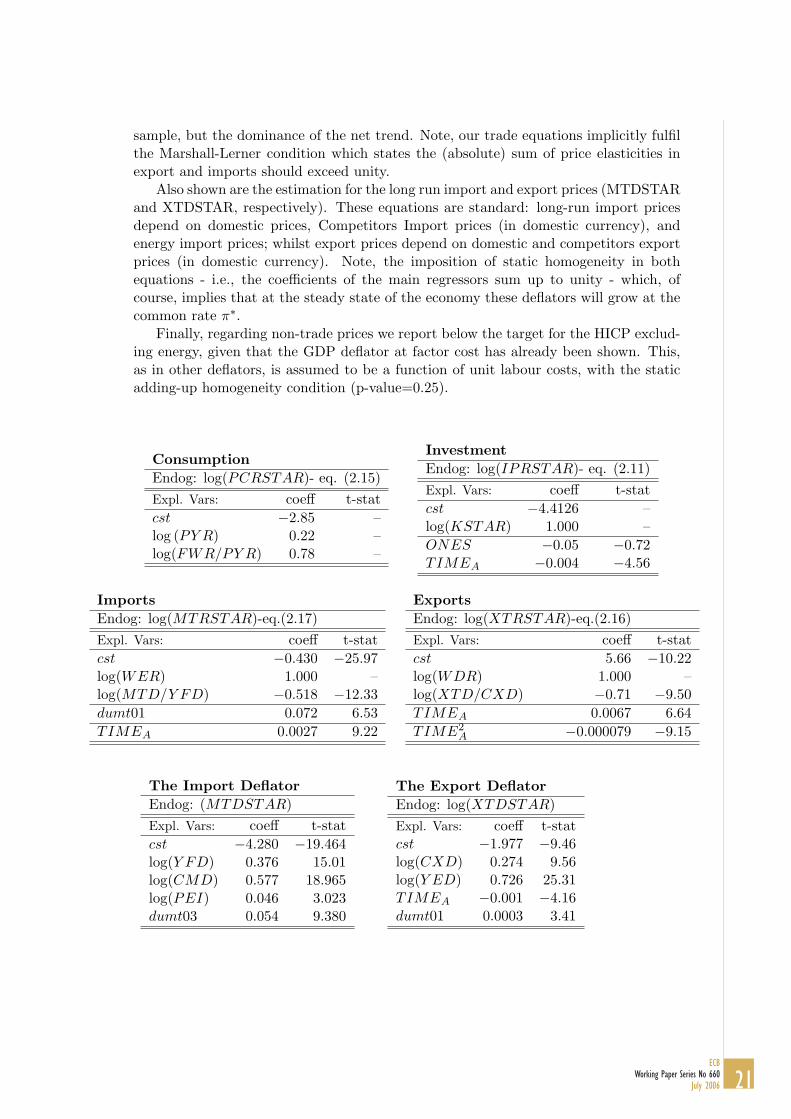
sample, but the dominance of the net trend. Note, our trade equations implicitly fulfilthe Marshall-Lerner condition which states the (absolute) sum of price elasticities inexport and imports should exceed unity.

Also shown are the estimation for the long run import and export prices (MTDSTARand XTDSTAR, respectively). These equations are standard: long-run import pricesdepend on domestic prices, Competitors Import prices (in domestic currency), andenergy import prices; whilst export prices depend on domestic and competitors exportprices (in domestic currency). Note, the imposition of static homogeneity in bothequations - i.e., the coefficients of the main regressors sum up to unity - which, ofcourse, implies that at the steady state of the economy these deflators will grow at thecommon rate π∗.

Finally, regarding non-trade prices we report below the target for the HICP exclud-ing energy, given that the GDP deflator at factor cost has already been shown. This,as in other deflators, is assumed to be a function of unit labour costs, with the staticadding-up homogeneity condition (p-value=0.25).

ConsumptionEndog: log(PCRSTAR)- eq. (2.15)Expl. Vars: coeff t-statcst −2.85 –log (PY R) 0.22 –log(FWR/PY R) 0.78 –

InvestmentEndog: log(IPRSTAR)- eq. (2.11)Expl. Vars: coeff t-statcst −4.4126 –log(KSTAR) 1.000 –ONES −0.05 −0.72TIMEA −0.004 −4.56

ImportsEndog: log(MTRSTAR)-eq.(2.17)Expl. Vars: coeff t-statcst −0.430 −25.97log(WER) 1.000 –log(MTD/Y FD) −0.518 −12.33dumt01 0.072 6.53TIMEA 0.0027 9.22

ExportsEndog: log(XTRSTAR)-eq.(2.16)Expl. Vars: coeff t-statcst 5.66 −10.22log(WDR) 1.000 –log(XTD/CXD) −0.71 −9.50TIMEA 0.0067 6.64TIME2

A −0.000079 −9.15

The Import DeflatorEndog: (MTDSTAR)Expl. Vars: coeff t-statcst −4.280 −19.464log(Y FD) 0.376 15.01log(CMD) 0.577 18.965log(PEI) 0.046 3.023dumt03 0.054 9.380

The Export DeflatorEndog: log(XTDSTAR)Expl. Vars: coeff t-statcst −1.977 −9.46log(CXD) 0.274 9.56log(Y ED) 0.726 25.31TIMEA −0.001 −4.16dumt01 0.0003 3.41

21ECB


HICP (Excluding Energy)Endog: log(HEXPSTAR)Expl. Vars: coeff t-statcst 4.73 –log (Y FD) 0.90 –log (MTD) 0.10 –TIMEA −0.004 −15.24TIME2

A 0.000025 11.20

3.3.2 Short-run Dynamics

Consumption, in the short-run is driven by its own dynamics, growth in real disposableincome, and unemployment. Note the unemployment rate was statistically insignificant(this may be due to collinearity with disposable income, since they both essentially cap-ture the role of liquidity-constrained consumer) but has been retained for reasons re-lating to simulation properties. Similarly, the long-run error correction is insignificant;this reflects our general difficulties in pinning down the long run consumption profileof the Italian economy, which may be related in the past to the effects of financial lib-eralization, public debt positions and different inflation and tax regimes: identificationof these effects however proved problematic.

Real private consumption

Endog: ∆log (PCR)Expl. Vars: coeff. t-statcst 0.0016 1.46∆ log (PCR(−1)) 0.558 4.72∆ log (PY R) 0.124 2.06∆ log (URX(−2/100) −0.02 −0.99

log(PCR(−1))− log (PCRSTAR(−1)) −0.012 1.46R2 = 0.63, DW = 1.88, σε = 0.005


ITALY

Real Private Consumption Residual

-3.0%

-2.0%

-1.0%

0.0%

1.0%

2.0%

3.0%

1990

Q1

1991

Q1

1992

Q1

1993

Q1

1994

Q1

1995

Q1

1996

Q1

1997

Q1

1998

Q1

1999

Q1

2000

Q1

2001

Q1

2002

Q1

2003

Q1

Contributions to the growth rate of private consumption

-5.0

-4.0

-3.0

-2.0

-1.0

0.0

1.0

2.0

3.0

4.0

1993A 1994A 1995A 1996A 1997A 1998A 1999A 2000A 2001A 2002A 2003A

Residual Real Disposable Income Unempl. Rate Other

Real Wealth Real Private Consump.

23ECB


3.3.3 Real private non-housing investment

The specification used for investment is a very simple accelerator one, with a long rundefined by IPRSTAR. However, other variables have considerable indirect effects, as itcan be seen from the contribution chart. For instance the real cost of capital producessome impact on investment dynamics through the error correction specification.

Real private non-housing investment

Endog: ∆log (IPR)Expl. Vars: coeff. t-statcst 0.0018 0.35∆ log (IPR(−1)) 0.320 2.29∆ log (IPR(−2)) 0.275 2.94∆ log (Y ER) 0.547 0.35dumt031 −0.134 −4.73

log(IPR(−1))− log (IPRSTAR(−1)) −0.06 −1.07R2 = 0.53, DW = 2.17, σε = 0.03

ITALY

Real Private Non-Housing Investment Residual

-6.0%

-4.0%

-2.0%

0.0%

2.0%

4.0%

6.0%

1990Q

1

1991Q

1

1992Q

1

1993Q

1

1994Q

1

1995Q

1

1996Q

1

1997Q

1

1998Q

1

1999Q

1

2000Q

1

2001Q

1

2002Q

1

2003Q

1


Contributions to the growth rate of real investment

-10.0

-5.0

0.0

5.0

10.0

15.0

1993A 1994A 1995A 1996A 1997A 1998A 1999A 2000A 2001A 2002A 2003A

Residual Real GDP User Cost Of Capital Nominal wages

GDP deflator Other Real Investment

3.3.4 Harmonised Index of Consumer Prices

For simulation purposes, the HICP is not strictly needed since it is essentially a passthrough of other prices. However, it is of course used in the context of projectionexercises. In projections, the IT-MCM comprises three additional HICP variables:total HICP, HEG (HICP energy) and HEXP (HICP excluding energy. HEXP, thesingle behavioural equation of the three, is determined by its own lags and those ofthe GDP deflator at factor cost, import prices, and, since the HICP series were notseasonally adjusted, seasonal dummies.

25ECB


HICP excluding energy (HEXP)

Endog: ∆log (HEXP )Expl. Vars: coeff. t-statcst 0.001 0.84∆ log (HEXP (−2)) −0.626 3.48∆ log (Y FD(−2) −0.036 −0.33∆ log (Y FD(−3)) −0.009 −0.06∆ log (MTD) −0.005 −0.25DUMMY Q1 0.003 2.52DUMMY Q2 0.004 2.51DUMMY Q3 −0.0008 −0.55

log(HEXP (−3))− log (HEXPSTAR(−3)) −0.142 −1.40R2 = 0.85, DW = 1.31, σε = 0.003

ITALY

HICP Excluding Energy Residual

-1.5%

-1.0%

-0.5%

0.0%

0.5%

1.0%

1.5%

1990

Q1

1991

Q1

1992

Q1

1993

Q1

1994

Q1

1995

Q1

1996

Q1

1997

Q1

1998

Q1

1999

Q1

2000

Q1

2001

Q1

2002

Q1

2003

Q1


Contributions to the growth rate of HICP ex-energy

-3.0

-2.0

-1.0

0.0

1.0

2.0

3.0

4.0

5.0

6.0

1993A 1994A 1995A 1996A 1997A 1998A 1999A 2000A 2001A 2002A 2003A

residual GDP deflator at factor cost Import deflator other HICP-ex inflation

3.3.5 Trade: Volumes and Prices

The dynamics of real exports demand depend upon its own lags, world demand, rela-tive prices and the real exchange rate. Imports demand are largely the correspondingequivalent of this. As regards trade prices, export prices are a dynamic function oftheir own lags, the GDP deflator at factor cost, and competitiveness. The dynamics ofimport prices, similarly, are a function of its own lags, competitiveness and the priceof imported energy products.

Real exports

Endog: ∆ log (XTR)Expl. Vars: coeff. t-statcst −0.016 −2.16∆ log (XTR(−1)) −0.207 −1.09∆ log (WDR) 1.729 3.18∆ log

(XTDCXD (−4)

)−0.175 −1.67

∆ log (EEN) 0.743 1.87

log(XTR(−1))− log (XTRSTAR(−1)) −0.431 −1.69R2 = 0.25, DW = 1.72, σε = 0.031

27ECB


ITALY

Real Exports Residual

-10.0%

-8.0%

-6.0%

-4.0%

-2.0%

0.0%

2.0%

4.0%

6.0%

8.0%

10.0%

1990

Q1

1991

Q1

1992

Q1

1993

Q1

1994

Q1

1995

Q1

1996

Q1

1997

Q1

1998

Q1

1999

Q1

2000

Q1

2001

Q1

2002

Q1

2003

Q1

Contributions to the growth rate of real exports

-10.0

-5.0

0.0

5.0

10.0

15.0

1993A 1994A 1995A 1996A 1997A 1998A 1999A 2000A 2001A 2002A 2003A

Residual World Demand CXD Exchange Rate

Other Export Deflator Real exports


Real imports

Endog: ∆ log (MTR)Expl. Vars: coeff. t-statcst −0.0027 −1.004∆ log (MTR(−1)) −0.299 −2.97∆ log (WER) 1.932 5.04∆ log (WER(−1)) 0.83 3.83∆ log (MTD/Y FD(−4)) −0.069 −1.04∆ log (EEN0(−1)) −0.277 −1.94

log(MTR(−1))− log (MTRSTAR(−1)) −0.077 −1.44R2 = 0.73, DW = 2.24, σε = 0.019

ITALY

Real Imports Residual

-6.0%

-4.0%

-2.0%

0.0%

2.0%

4.0%

6.0%

8.0%

1990

Q1

1991

Q1

1992

Q1

1993

Q1

1994

Q1

1995

Q1

1996

Q1

1997

Q1

1998

Q1

1999

Q1

2000

Q1

2001

Q1

2002

Q1

2003

Q1

29ECB


Contributions to the growth rate of real imports

-15.0

-10.0

-5.0

0.0

5.0

10.0

15.0

1993A 1994A 1995A 1996A 1997A 1998A 1999A 2000A 2001A 2002A 2003A

Residual Import Demand Ind. GDP Defl. at fact. Cost

Import Deflator Exchange Rate Other

Real Imports

Export deflator

Endog: ∆log (XTD)Expl. Vars: coeff. t-statcst −0.001 −0.81∆ log (XTD(−1)) −0.41 3.94∆ log (CXD) 0.209 3.81∆ log (Y FD) 0.649 3.08

log(

XTD(−1)

XTDSTAR(−1)

)−0.295 −3.6

R2 = 0.77, DW = 2.19, σε = 0.008


ITALY

Export Deflator Residual

-4.0%

-3.0%

-2.0%

-1.0%

0.0%

1.0%

2.0%

3.0%

4.0%

1990

Q1

1991

Q1

1992

Q1

1993

Q1

1994

Q1

1995

Q1

1996

Q1

1997

Q1

1998

Q1

1999

Q1

2000

Q1

2001

Q1

2002

Q1

Contributions to the growth rate of export deflator

-6.0

-4.0

-2.0

0.0

2.0

4.0

6.0

8.0

10.0

12.0

1993A 1994A 1995A 1996A 1997A 1998A 1999A 2000A 2001A 2002A 2003A

Residual GDP fact. cost CXD Other Export Deflator

31ECB


Import deflator

Endog: ∆log (MTD)Expl. Vars: coeff. t-statcst −0.0034 −2.00∆ log (MTD(−1)) 0.244 5.28∆ log (MTD(−2)) 0.137 3.05∆ log (Y FD(−1)) 0.562 3.34∆ log (CMD) 0.435 10.38∆ log (PEI) 0.07 4.34

log(

MTD(−1)

MTDSTAR(−1)

)−0.5 −4.73

R2 = 0.92, DW = 2.22, σε = 0.007

ITALY

Import Deflator Residual

-3.0%

-2.0%

-1.0%

0.0%

1.0%

2.0%

3.0%

1990

Q1

1991

Q1

1992

Q1

1993

Q1

1994

Q1

1995

Q1

1996

Q1

1997

Q1

1998

Q1

1999

Q1

2000

Q1

2001

Q1

2002

Q1


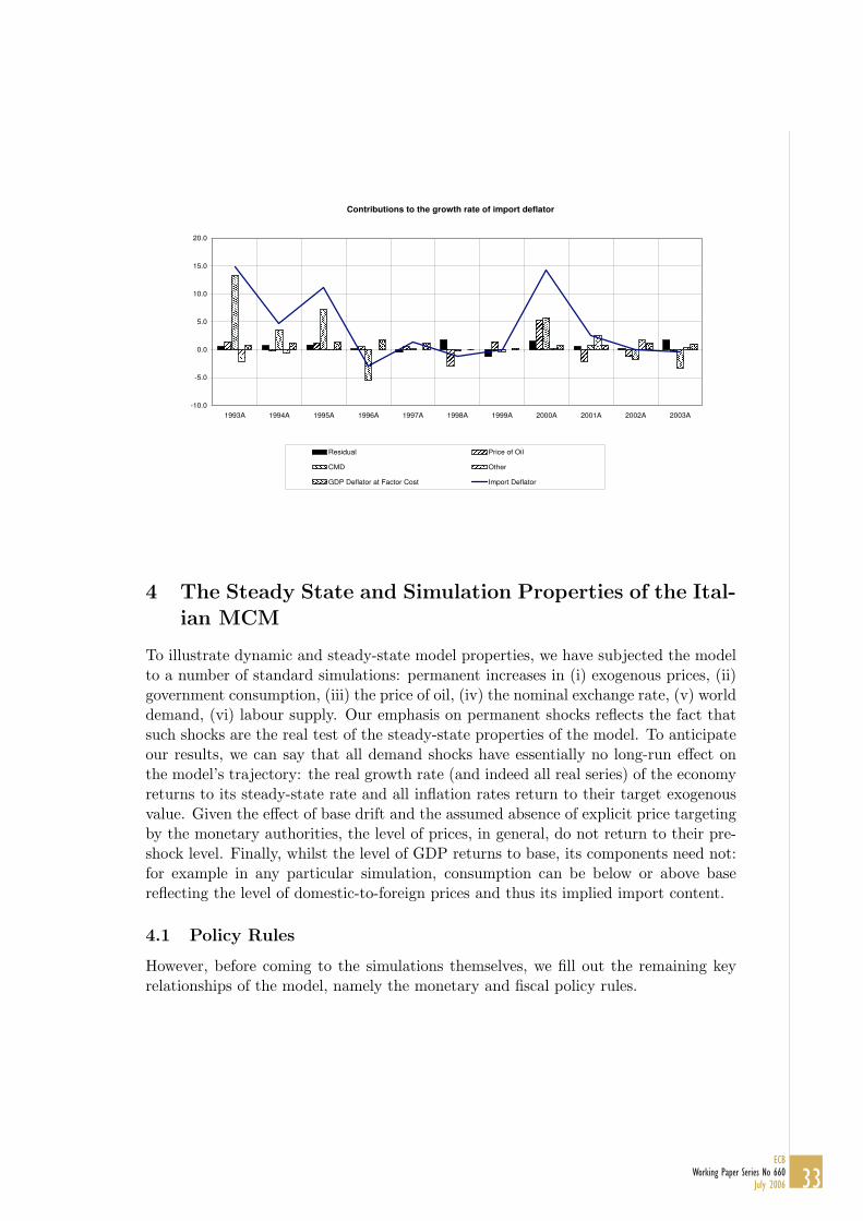
Contributions to the growth rate of import deflator

-10.0

-5.0

0.0

5.0

10.0

15.0

20.0

1993A 1994A 1995A 1996A 1997A 1998A 1999A 2000A 2001A 2002A 2003A

Residual Price of Oil

CMD Other

GDP Deflator at Factor Cost Import Deflator

4 The Steady State and Simulation Properties of the Ital-ian MCM

To illustrate dynamic and steady-state model properties, we have subjected the modelto a number of standard simulations: permanent increases in (i) exogenous prices, (ii)government consumption, (iii) the price of oil, (iv) the nominal exchange rate, (v) worlddemand, (vi) labour supply. Our emphasis on permanent shocks reflects the fact thatsuch shocks are the real test of the steady-state properties of the model. To anticipateour results, we can say that all demand shocks have essentially no long-run effect onthe model’s trajectory: the real growth rate (and indeed all real series) of the economyreturns to its steady-state rate and all inflation rates return to their target exogenousvalue. Given the effect of base drift and the assumed absence of explicit price targetingby the monetary authorities, the level of prices, in general, do not return to their pre-shock level. Finally, whilst the level of GDP returns to base, its components need not:for example in any particular simulation, consumption can be below or above basereflecting the level of domestic-to-foreign prices and thus its implied import content.

4.1 Policy Rules

However, before coming to the simulations themselves, we fill out the remaining keyrelationships of the model, namely the monetary and fiscal policy rules.

33ECB


4.1.1 Monetary Policy Rule

The Central bank is assumed to operate a Taylor-type rule and adjusts nominal interestrates to inflation deviations form the target and to the output gap (or more strictly,output growth6):

STIt = ρSTIt−1 +

(1− ρ)400[γ + n + π∗ + 1.5

(PCDt/PCDt−1 − π∗

)+0.5

(Y ERt/Y ERt−1−γ − n

)]

−(1− ρ)

where the degree of interest-rate smoothing, ρ is typically set to 0.5. Clearly, inthe long run, when the growth rate of GDP and inflation equate to their long runvalue target, the short-term rate is equal to the nominal growth rate of the economy(γ+n+π∗). Of course, in projection exercises, the nominal interest rate is held constant(as is the exchange rate).

4.1.2 Fiscal Policy Rule

The fiscal rule used in the model is flexible but straightforward:

PDX = ρPDX ·PDXt−1 + λ1 (GDN/4 · Y EN −D∗)

+λ2

((GLN/4 · Y EN)t−1 − (GLN/4 · Y EN)t−2

)

where parameter λ measures the feedback of tax rates to deviations from policyobjectives, whether that be the debt (D*), the first deviation term, or the dynamicsof deficit ratios, the second. The values of these fiscal targets were set in line withhistorical averages, which is just over 100 percent of GDP for Italy. The values ofλ1 and λ2 were set to which appeared to generate plausible and stable tax trajectories,namely 0.1 and 0.01 respectively. Parameter ρPDXallows us to specify the rule as aproportional or integral control, although in most circumstance, we choose the latter.

4.2 Steady State

The procedure for setting up a steady state baseline is quite straight forward. First wedivide all variables (excluding residuals) contained in the model into their underlyingcategories: real, nominal, demographic, constant etc. We then apply, to the end-point of the historical series, relevant extrapolations of these growth rates. Second,the out-of-sample residuals of all the equations are then inverted to produce a baseline

6Both output growth and the actual output gap can be used and results on the latter are available onrequest. However, the latter, tends to engender somewhat slower model dynamics, so we chose here tofocus on the output growth concept. Indeed, this is also the case for the other MCM models and so wefor consistency purposes we followed that approach. Moreover, much of the recent work on estimatingpolicy rules has in fact used output growth instead of output gaps (which can be highly sensitive todetrending and calculation methods), see the recent work by Orphanides and other authors.


consistent with these implied paths. The model is then explicitly solved, to check forconsistency, stability and that, in the absence of any pertubation, that the model doesindeed return to a steady state with given growth characteristics. Once we have deriveda model which displays suitable characteristics, we then apply standard simulations toensure acceptable simulation properties. These are discussed below.

4.3 Illustrative Simulations

4.3.1 Shocks to Price and Nominal Variables

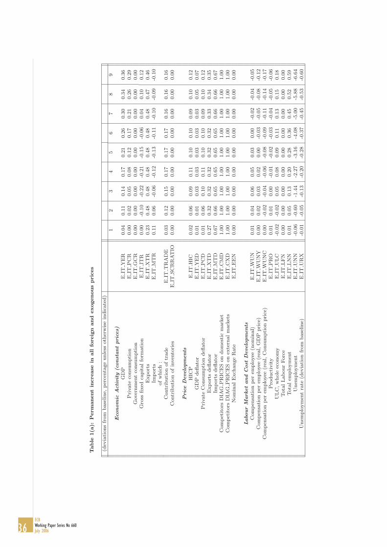
The purpose of this shock is to check that nominal neutrality holds in the steadystate of the model. Accordingly, all exogenous and foreign prices of the model (e.g.oil, imported energy, competitors’ prices, etc.) have been increased by 1% above thebaseline. As expected, all of the endogenous prices react positively and converge to ahigher steady state, in a fairly monotonic manner, with an eventual full pass-throughof +1%. The shock also has an impact on the real economy in the short run: pricecompetitiveness improves and GDP rises, initially. In particular, real trade variableskeep on adjusting as long as relative prices (domestic/foreign) depart from their steadystate (as they will when a positive output gap arises). The initial effects vanish asdomestic agents adjust their own prices, and the operation of tax and interest ratecome into effect. In the long run, all real variables of the economy go back to theirbaseline, as shown in the charts below. Inflation rates (for the various deflators) returnto their long run rate, although, as said, there is necessarily a level effect on prices (of1%).

Economic Activity - Domestic Demand

(%-deviation from Steady-State)

-0.5

-0.4

-0.3

-0.2

-0.1

0.0

0.1

0.2

0.3

0.4

0.5

1 11 21 31 41 51 61 71 81 91 101 111 121 131 141 151

GDP Private consumption Gross fixed capital formation

Domestic Prices and Trade Deflators


0.00

0.10

0.20

0.30

0.40

0.50

0.60

0.70

0.80

0.90

1.00

1.10

1.20

1.30

1.40

1.50

1 11 21 31 41 51 61 71 81 91 101 111 121 131 141 151

GDP deflator Private consumption deflator Export deflator Import deflator

4.3.2 Permanent shock to government consumption

In this simulation, real government consumption has been increased permanently by1% above baseline GDP. The mechanics of this type of demand shock are relativelywell known: through the operation of the multiplier and accelerator mechanism, theincrease in public expenditure raises, respectively, consumption and investment andthus the overall level of output with the initial GDP multiplier effect is around 1%rising to a maximum of 1.5% (for a closed-economy model above-unity multipliers arenot uncommon). Given rigidities in price and wage setting these effects persist forseveral quarters yielding higher real wages and additional employment.

35ECB


Table

1(a

):Perm

anent

increase

inall

foreig

nand

exogenous

pric

es

(dev

iati

ons

from

base

line,

per

centa

ge

unle

ssoth

erw

ise

indic

ate

d)

12

34

56

78

9Eco

nom

icActivity

(const

antpri

ces)

GD

PE

ITY

ER

0.0

40.1

10.1

40.1

70.2

10.2

60.3

00.3

40.3

6P

rivate

consu

mpti

on

EIT

PC

R0.0

00.0

20.0

50.0

80.1

20.1

70.2

10.2

60.2

9G

over

nm

ent

consu

mpti

on

EIT

GC

R0.0

00.0

00.0

00.0

00.0

00.0

00.0

00.0

00.0

0G

ross

fixed

capit

alfo

rmati

on

EIT

ITR

0.0

0-0

.10

-0.2

2-0

.21

-0.1

5-0

.06

0.0

40.1

00.1

2E

xport

sE

ITX

TR

0.2

30.4

80.4

80.4

80.4

80.4

80.4

80.4

70.4

6Im

port

sE

ITM

TR

0.1

10.0

6-0

.06

-0.1

2-0

.13

-0.1

1-0

.10

-0.0

9-0

.10

ofw

hic

h:

Contr

ibuti

on

oftr

ade

EIT

TR

AD

E0.0

30.1

20.1

50.1

70.1

70.1

70.1

60.1

60.1

6C

ontr

ibuti

on

ofin

ven

tori

esE

ITSC

RR

AT

IO0.0

00.0

00.0

00.0

00.0

00.0

00.0

00.0

00.0

0

Pri

ceD

evelo

pm

ents

HIC

PE

ITH

IC0.0

20.0

60.0

90.1

10.1

00.1

00.0

90.1

00.1

2G

DP

defl

ato

rE

ITY

ED

0.0

10.0

10.0

30.0

30.0

30.0

30.0

30.0

50.0

7P

rivate

Consu

mpti

on

defl

ato

rE

ITP

CD

0.0

10.0

60.1

00.1

10.1

00.1

00.0

90.1

00.1

2E

xport

sdefl

ato

rE

ITX

TD

0.2

70.3

20.3

20.3

20.3

20.3

20.3

30.3

40.3

5Im

port

sdefl

ato

rE

ITM

TD

0.6

70.6

60.6

50.6

50.6

50.6

50.6

60.6

60.6

7C

om

pet

itors

DIA

GP

RIC

ES

on

dom

esti

cm

ark

etE

ITC

MD

1.0

01.0

01.0

01.0

01.0

01.0

01.0

01.0

01.0

0C

om

pet

itors

DIA

GP

RIC

ES

on

exte

rnalm

ark

ets

EIT

CX

D1.0

01.0

01.0

01.0

01.0

01.0

01.0

01.0

01.0

0N

om

inalE

xch

ange

Rate

EIT

EE

N0.0

00.0

00.0

00.0

00.0

00.0

00.0

00.0

00.0

0

Labo

ur

Mark

etand

Cost

Develo

pm

ents

Com

pen

sati

on

per

emplo

yee

(nom

inal)

EIT

WU

N0.0

10.0

40.0

60.0

50.0

30.0

0-0

.02

-0.0

4-0

.05

Com

pen

sati

on

per

emplo

yee

(rea

l,G

DP

pri

ce)

EIT

WU

NY

0.0

00.0

20.0

30.0

20.0

0-0

.03

-0.0

5-0

.08

-0.1

2C

om

pen

sati

on

per

emplo

yee

(rea

l,C

onsu

mpti

on

pri

ce)

EIT

WU

NC

0.0

0-0

.02

-0.0

4-0

.06

-0.0

8-0

.09

-0.1

1-0

.14

-0.1

7P

roduct

ivity

EIT

PR

O0.0

10.0

10.0

0-0

.01

-0.0

2-0

.03

-0.0

4-0

.05

-0.0

6U

LC

,w

hole

econom

yE

ITU

LC

-0.0

2-0

.02

0.0

50.0

80.0

90.1

10.1

30.1

50.1

8Tota

lLabour

Forc

eE

ITLFN

0.0

00.0

00.0

00.0

00.0

00.0

00.0

00.0

00.0

0Tota

lem

plo

ym

ent

EIT

LN

N0.0

10.0

50.1

30.2

00.2

80.3

60.4

50.5

20.5

9U

nem

plo

ym

ent

EIT

UN

N-0

.06

-0.6

0-1

.44

-2.2

7-3

.16

-4.0

8-5

.00

-5.8

8-6

.64

Unem

plo

ym

ent

rate

(dev

iati

on

from

base

line)

EIT

UR

X-0

.01

-0.0

5-0

.13

-0.2

0-0

.28

-0.3

7-0

.45

-0.5

3-0

.60


Table

1(a

):Perm

anent

increase

inall

foreig

nand

exogenous

pric

es

(dev

iati

ons

from

base

line,

per

centa

ge

unle

ssoth

erw

ise

indic

ate

d)

12

34

56

78

9D

isposa

ble

Inco

me

(nom

inal)

&Tota

lW

ealth

Dis

posa

ble

inco

me

EIT

PY

N0.0

40.1

30.1

90.2

30.3

00.3

80.4

70.5

30.5

7R

ealdis

posi

ble

Inco

me

EIT

PY

R0.0

30.0

70.0

90.1

20.1

90.2

80.3

70.4

30.4

5C

om

pen

sati

on

ofem

plo

yee

sE

ITW

IN0.0

10.0

90.1

90.2

50.3

10.3

70.4

30.4

90.5

4Tra

nsf

ers

from

GalG

ov.

EIT

TR

N0.0

40.1

20.1

70.2

00.2

40.2

80.3

30.3

80.4

3O

ther

Per

sonalin

com

eE

ITO

PN

0.0

30.0

80.0

80.0

80.0

90.1

10.1

20.1

40.1

6D

ires

tTaxes

(inc.

SSC

)E

ITP

DN

-0.0

1-0

.03

-0.0

2-0

.03

-0.0

9-0

.20

-0.3

1-0

.36

-0.3

1Tota

lW

ealt

hE

ITFW

N0.0

40.0

30.0

50.0

60.0

70.0

80.1

10.1

50.2

0R

ealTota

lW

ealt

hE

ITFW

R0.0

3-0

.02

-0.0

5-0

.05

-0.0

3-0

.01

0.0

20.0

50.0

8Savin

gra

tio

EIT

SR

AT

IO0.0

20.0

30.0

10.0

10.0

10.0

10.0

20.0

20.0

1N

etFore

ign

Ass

ets

(rati

o)

EIT

NFA

RAT

IO-0

.05

-0.0

8-0

.03

0.0

30.1

00.1

60.2

30.2

90.3

5Fir

ms

and

Inte

rest

Rate

Capit

alSto

ckE

ITK

SR

0.0

00.0

0-0

.01

-0.0

3-0

.04

-0.0

4-0

.04

-0.0

3-0

.02

Rea

lC

ost

ofC

apit

al(a

ver

age)

EIT

CC

R0.9

01.6

40.8

00.7

50.5

00.3

20.2

90.3

00.2

93-m

onth

inte

rest

rate

EIT

ST

I0.0

50.1

10.0

70.0

30.0

10.0

10.0

20.0

30.0

410-y

ear

long-t

erm

inte

rest

rate

EIT

LT

I0.0

40.1

00.0

60.0

40.0

20.0

10.0

20.0

30.0

3

Public

Sec

tor

GalG

ov.

Com

pen

sati

on

ofE

mplo

yee

sE

ITP

DN

-0.0

1-0

.03

-0.0

2-0

.03

-0.0

9-0

.20

-0.3

1-0

.36

-0.3

1Tra

nfe

rsfr

om

galG

ov.

EIT

TR

N0.0

40.1

20.1

70.2

00.2

40.2

80.3

30.3

80.4

3O

ther

Gov.

Net

Rev

enues

EIT

OG

N1.0

01.0

01.0

01.0

01.0

01.0

01.0

01.0

01.0

0D

ires

tTaxes

(inc.

SSC

)E

ITP

DX

-0.0

4-0

.12

-0.1

6-0

.20

-0.3

0-0

.44

-0.5

9-0

.68

-0.6

8O

ther

Dir

ect

Taxes

EIT

OD

N0.0

20.0

60.0

60.0

70.0

80.1

00.1

20.1

30.1

5In

dir

ect

Taxes

less

Subsi

die

sE

ITT

IN0.0

50.0

70.0

80.1

10.1

40.1

80.2

30.2

80.3

2G

en.

Gov.

Net

Deb

tE

ITG

DN

0.0

00.0

90.1

50.1

70.1

80.2

00.2

60.3

50.4

5G

en.

Gov.

Net

Len

din

g(%

ofG

DP

)E

ITG

LN

RAT

IO-0

.02

-0.1

0-0

.05

-0.0

1-0

.01

-0.0

4-0

.08

-0.1

1-0

.11

Gen

.G

ov.

Net

Deb

t(%

ofG

DP

)E

ITG

DN

RAT

IO-0

.04

-0.0

4-0

.02

-0.0

3-0

.07

-0.0

9-0

.08

-0.0

30.0

3

37ECB


However, a number of mechanisms react such as to dissipate the positive effect ofthis shock. First, there is a deterioration of net trade, since output growth boostsimport demand and, adverse competitiveness effects, rising from rising domestic priceand cost pressure, curtail export demand. Second, there is the operation of tighterfiscal and monetary policies to contain the adverse movements in fiscal ratios, andinflation and output targets. In the long run, therefore, output and employment returnto base, but consumption falls below base due to changes in relative prices (foreign anddomestic) for a given level of import content. Finally, steady-state inflation necessarilyreturns to its target value there still remains price-level drift.

Economic activity - Consumption


-2.5

-2.0

-1.5

-1.0

-0.5

0.0

0.5

1.0

1.5

2.0

1 11 21 31 41 51 61 71 81 91 101 111 121 131

Private Consumption GDP Gross fixed capital formation

Economic Activity - Trade


-1.50

-1.00

-0.50

0.00

0.50

1.00

1.50

1 11 21 31 41 51 61 71 81 91 101 111 121 131

Real exports Real imports

Domestic Prices


-0.50

0.00

0.50

1.00

1.50

2.00

2.50

1 11 21 31 41 51 61 71 81 91 101 111 121 131

YED PCD

employment

Labour Market


-3.0

-2.0

-1.0

0.0

1.0

2.0

3.0

1 11 21 31 41 51 61 71 81 91 101 111 121 131

Total employmentUnemployment rate (deviation from baseline)

4.3.3 Permanent increase in oil prices

This simulation assumes that oil prices are increased permanently by 20% above base-line. This has an increase in the import deflator by 0.23% during the first year, andthe increase feeds more into the private consumption deflator (the GDP deflator doesnot depend directly on import prices) which increase by 0.16 % above baseline, in thesecond year. The decline in real wages, 0.12% below baseline, causes the decline in realdisposable income. This, with real financial wealth being a key determinant of privateconsumption, also declines in the short to medium run. The increase in prices has anegative effect on investment which is also negatively affecting demand. The increase inimport prices and the slowdown in demand cause imports to decrease. Detailed resultsare reported below.


Table

2(a

):Perm

anent

increase

ingovernm

ent

consu

mpti

on

(dev

iati

ons

from

base

line,

per

centa

ge

unle

ssoth

erw

ise

indic

ate

d)

12

34

56

78

9Eco

nom

icActivity

(const

antpri

ces)

GD

PE

ITY

ER

0.9

51.0

41.1

51.1

91.2

51.3

41.4

41.5

11.5

3P

rivate

consu

mpti

on

EIT

PC

R0.0

90.3

30.5

50.6

60.7

10.7

80.8

91.0

21.1

0G

over

nm

ent

consu

mpti

on

EIT

GC

R5.5

35.5

35.5

35.5

35.5

35.5

35.5

35.5

35.5

3G

ross

fixed

capit

alfo

rmati

on

EIT

ITR

0.1

30.0

60.2

7-0

.01

0.1

40.6

11.0

11.1

20.9

7E

xport

sE

ITX

TR

0.0

0-0

.05

-0.0

50.0

10.0

40.0

40.0

0-0

.07

-0.1

5Im

port

sE

ITM

TR

0.4

80.5

70.7

80.7

40.7

90.9

61.1

11.1

41.0

4ofw

hic

h:

Contr

ibuti

on

oftr

ade

EIT

TR

AD

E-0

.13

-0.1

8-0

.24

-0.2

0-0

.21

-0.2

6-0

.31

-0.3

4-0

.34

Contr

ibuti

on

ofin

ven

tori

esE

ITSC

RR

AT

IO0.0

00.0

00.0

00.0

00.0

00.0

00.0

00.0

00.0

0

Pri

ceD

evelo

pm

ents

HIC

PE

ITH

IC0.0

00.0

30.0

90.0

7-0

.02

-0.0

9-0

.07

0.0

30.1

9G

DP

defl

ato

rE

ITY

ED

0.0

30.1

40.0

80.0

0-0

.06

-0.0

40.0

50.1

90.3

6P

rivate

Consu

mpti

on

defl

ato

rE

ITP

CD

0.0

00.0

20.0

90.0

9-0

.01

-0.1

0-0

.09

0.0

10.1

8E

xport

sdefl

ato

rE

ITX

TD

0.0

10.1

30.0

1-0

.05

-0.0

7-0

.03

0.0

50.1

60.2

9Im

port

sdefl

ato

rE

ITM

TD

0.0

00.0

70.0

1-0

.03

-0.0

4-0

.02

0.0

20.0

80.1

5C

om

pet

itors

Pri

ces

on

dom

esti

cm

ark

etE

ITC

MD

0.0

00.0

00.0

00.0

00.0

00.0

00.0

00.0

00.0

0C

om

pet

itors

Pri

ces

on

exte

rnalm

ark

ets

EIT

CX

D0.0

00.0

00.0

00.0

00.0

00.0

00.0

00.0

00.0

0N

om

inalE

xch

ange

Rate

EIT

EE

N0.0

00.0

00.0

00.0

00.0

00.0

00.0

00.0

00.0

0

Labo

ur

Mark

etand

Cost

Develo

pm

ents

Com

pen

sati

on

per

emplo

yee

(nom

inal)

EIT

WU

N0.1

50.3

50.2

50.0

3-0

.20

-0.3

4-0

.37

-0.3

3-0

.25

Com

pen

sati

on

per

emplo

yee

(rea

l,G

DP

pri

ce)

EIT

WU

NY

0.1

20.2

10.1

60.0

3-0

.14

-0.3

0-0

.42

-0.5

2-0

.61

Com

pen

sati

on

per

emplo

yee

(rea

l,C

onsu

mpti

on

pri

ce)

EIT

WU

NC

0.1

50.3

30.1

5-0

.06

-0.1

8-0

.24

-0.2

8-0

.34

-0.4

3P

roduct

ivity

EIT

PR

O0.1

80.0

5-0

.03

-0.1

1-0

.15

-0.1

7-0

.19

-0.2

1-0

.23

ULC

,w

hole

econom

yE

ITU

LC

-0.5

50.1

30.3

80.4

60.4

10.3

60.3

90.5

10.6

8Tota

lLabour

Forc

eE

ITLFN

0.0

00.0

00.0

00.0

00.0

00.0

00.0

00.0

00.0

0Tota

lem

plo

ym

ent

EIT

LN

N0.2

40.8

21.2

81.6

21.8

62.0

52.2

22.3

72.4

7U

nem

plo

ym

ent

EIT

UN

N-2

.64

-9.1

9-1

4.4

0-1

8.2

0-2

0.8

4-2

2.9

7-2

4.8

9-2

6.5

6-2

7.7

3U

nem

plo

ym

ent

rate

(dev

iati

on

from

base

line)

EIT

UR

X-0

.24

-0.8

2-1

.29

-1.6

3-1

.87

-2.0

6-2

.23

-2.3

8-2

.48

39ECB


Table

2(a

):Perm

anent

increase

ingovernm

ent

consu

mpti

on

(dev

iati

ons

from

base

line,

per

centa

ge

unle

ssoth

erw

ise

indic

ate

d)

12

34

56

78

9D

isposa

ble

Inco

me

(nom

inal)

&Tota

lW

ealth

Dis

posa

ble

inco

me

EIT

PY

N0.6

50.6

60.1

6-0

.54

-0.9

4-0

.80

-0.1

80.5

91.1

7R

ealdis

posi

ble

Inco

me

EIT

PY

R0.6

50.6

40.0

7-0

.62

-0.9

3-0

.70

-0.0

90.5

71.0

0C

om

pen

sati

on

ofem

plo

yee

sE

ITW

IN0.3

91.1

71.5

31.6

51.6

61.7

11.8

42.0

32.2

2Tra

nsf

ers

from

GalG

ov.

EIT

TR

N0.9

81.1

81.2

41.1

81.1

91.3

01.4

91.7

11.9

0O

ther

Per

sonalin

com

eE

ITO

PN

0.6

60.5

10.3

90.2

90.3

00.3

70.4

80.5

90.6

8D

ires

tTaxes

(inc.

SSC

)E

ITP

DN

0.4

61.6

43.6

95.9

37.2

77.1

05.6

83.8

82.6

1Tota

lW

ealt

hE

ITFW

N0.1

40.3

90.4

70.4

00.2

20.0

3-0

.06

-0.0

20.1

5R

ealTota

lW

ealt

hE

ITFW

R0.1

40.3

70.3

70.3

10.2

30.1

30.0

3-0

.03

-0.0

3Savin

gra

tio

EIT

SR

AT

IO0.5

30.4

90.3

50.2

60.2

90.3

70.4

10.4

00.3

6N

etfo

reig

nass

ets

(rati

o)

EIT

NFA

RAT

IO-0

.08

-0.2

0-0

.40

-0.6

1-0

.80

-1.0

2-1

.29

-1.5

7-1

.86

Fir

ms

and

Inte

rest

Rate

Capit

alSto

ckE

ITK

SR

0.0

10.0

10.0

20.0

30.0

30.0

50.1

00.1

60.2

1R

ealC

ost

ofC

apit

al(a

ver

age)

EIT

CC

R8.0

3-1

.40

5.0

51.4

5-0

.80

-1.1

3-0

.48

0.4

20.9

33-m

onth

inte

rest

rate

EIT

ST

I0.4

70.1

30.1

5-0

.04

-0.1

4-0

.05

0.1

10.2

20.2

610-y

ear

long-t

erm

inte

rest

rate

EIT

LT

I0.4

50.0

40.2

0-0

.01

-0.0

9-0

.04

0.0

70.1

70.2

2

Public

Sec

tor

GalG

ov.

Com

pen

sati

on

ofE

mplo

yee

sE

ITP

DN

0.4

61.6

43.6

95.9

37.2

77.1

05.6

83.8

82.6

1Tra

nfe

rsfr

om

galG

ov.

EIT

TR

N0.9

81.1

81.2

41.1

81.1

91.3

01.4

91.7

11.9

0O

ther

Gov.

Net

Rev

enues

EIT

OG

N0.0

00.0

00.0

00.0

00.0

00.0

00.0

00.0

00.0

0D

ires

tTaxes

(inc.

SSC

)E

ITP

DX

-0.1

40.7

32.6

44.8

66.1

85.9

44.4

02.4

51.0

6O

ther

Dir

ect

Taxes

EIT

OD

N0.6

60.4

90.3

80.3

00.3

00.3

80.4

70.5

50.6

1In

dir

ect

Taxes

less

Subsi

die

sE

ITT

IN1.1

61.3

61.5

41.5

01.4

91.5

81.7

71.9

92.1

8G

en.

Gov.

Net

Deb

tE

ITG

DN

0.9

91.8

72.4

12.2

81.6

00.8

60.5

00.7

01.3

5G

en.

Gov.

Net

Len

din

g(%

ofG

DP

)E

ITG

LN

RAT

IO-1

.45

-0.8

7-0

.39

0.3

80.8

30.7

10.1

9-0

.39

-0.8

0G

en.

Gov.

Net

Deb

t(%

ofG

DP

)E

ITG

DN

RAT

IO0.0

00.7

41.2

61.1

80.4

4-0

.47

-1.0

6-1

.07

-0.5

9


Table

3(a

):Perm

anent

oil

pric

esh

ock

(dev

iati

ons

from

base

line,

per

centa

ge

unle

ssoth

erw

ise

indic

ate

d)

12

34

56

78

9Eco

nom

icActivity

(const

antpri

ces)

GD

PE

ITY

ER

0.0

00.0

1-0

.03

-0.0

7-0

.07

-0.0

7-0

.05

-0.0

4-0

.04

Pri

vate

consu

mpti

on

EIT

PC

R0.0

0-0

.02

-0.0

8-0

.15

-0.2

1-0

.25

-0.2

5-0

.24

-0.2

4G

over

nm

ent

consu

mpti

on

EIT

GC

R0.0

00.0

00.0

00.0

00.0

00.0

00.0

00.0

00.0

0G

ross

fixed

capit

alfo

rmati

on

EIT

ITR

0.0

0-0

.19

-0.8

1-0

.91

-0.7

6-0

.60

-0.4

2-0

.31

-0.2

8E

xport

sE

ITX

TR

0.0

00.0

0-0

.02

-0.0

4-0

.05

-0.0

6-0

.07

-0.0

8-0

.09

Import

sE

ITM

TR

0.0

0-0

.24

-0.7

3-0

.83

-0.8

3-0

.80

-0.7

4-0

.70

-0.6

9ofw

hic

h:

Contr

ibuti

on

oftr

ade

EIT

TR

AD

E0.0

00.0

70.2

00.2

20.2

20.2

10.1

90.1

70.1

7C

ontr

ibuti

on

ofin

ven

tori

esE

ITSC

RR

AT

IO0.0

00.0

00.0

00.0

00.0

00.0

00.0

00.0

00.0

0

Pri

ceD

evelo

pm

ents

HIC

PE

ITH

IC0.0

10.1

90.3

10.3

70.4

10.4

20.4

40.4

60.4

8G

DP

defl

ato

rE

ITY

ED

0.0

00.0

30.0

80.1

00.1

30.1

50.1

70.1

90.2

1P

rivate

Consu

mpti

on

defl

ato

rE

ITP

CD

0.0

00.1

60.3

30.3

80.4

10.4

20.4

40.4

60.4

8E

xport

sdefl

ato

rE

ITX

TD

0.0

00.0

10.0

50.0

70.0

80.1

00.1

10.1

30.1

4Im

port

sdefl

ato

rE

ITM

TD

0.2

31.4

31.1

91.3

01.3

31.3

41.3

51.3

61.3

6C

om

pet

itors

Pri

ces

on

dom

esti

cm

ark

etE

ITC

MD

0.0

00.0

00.0

00.0

00.0

00.0

00.0

00.0

00.0

0C

om

pet

itors

Pri

ces

on

exte

rnalm

ark

ets

EIT

CX

D0.0

00.0

00.0

00.0

00.0

00.0

00.0

00.0

00.0

0N

om

inalE

xch

ange

Rate

EIT

EE

N0.0

00.0

00.0

00.0

00.0

00.0

00.0

00.0

00.0

0

Labo

ur

Mark

etand

Cost

Develo

pm

ents

Com

pen

sati

on

per

emplo

yee

(nom

inal)

EIT

WU

N0.0

00.0

30.0

80.0

80.0

80.0

90.1

00.1

10.1

1C

om

pen

sati

on

per

emplo

yee

(rea

l,G

DP

pri

ce)

EIT

WU

NY

0.0

00.0

00.0

1-0

.02

-0.0

4-0

.06

-0.0

7-0

.08

-0.1

0C

om

pen

sati

on

per

emplo

yee

(rea

l,C

onsu

mpti

on

pri

ce)

EIT

WU

NC

0.0

0-0

.12

-0.2

5-0

.29

-0.3

2-0

.33

-0.3

4-0

.35

-0.3

7P

roduct

ivity

EIT

PR

O0.0

00.0

0-0

.01

-0.0

2-0

.02

-0.0

2-0

.02

-0.0

2-0

.03

ULC

,w

hole

econom

yE

ITU

LC

0.0

00.0

30.1

20.1

60.1

60.1

70.1

80.2

10.2

3Tota

lLabour

Forc

eE

ITLFN

0.0

00.0

00.0

00.0

00.0

00.0

00.0

00.0

00.0

0Tota

lem

plo

ym

ent

EIT

LN

N0.0

00.0

00.0

10.0

00.0

00.0

10.0

30.0

60.0

9U

nem

plo

ym

ent

EIT

UN

N0.0

0-0

.03

-0.1

6-0

.05

0.0

1-0

.09

-0.3

2-0

.64

-0.9

6U

nem

plo

ym

ent

rate

(dev

iati

on

from

base

line)

EIT

UR

X0.0

00.0

0-0

.01

0.0

00.0

0-0

.01

-0.0

3-0

.06

-0.0

9

41ECB


Table

3(b

):Perm

anent

oil

pric

esh

ock

(dev

iati

ons

from

base

line,

per

centa

ge

unle

ssoth

erw

ise

indic

ate

d)

12

34

56

78

9D

isposa

ble

Inco

me

(nom

inal)

&Tota

lW

ealth

Dis

posa

ble

inco

me

EIT

PY

N0.0

0-0

.03

-0.1

9-0

.36

-0.3

9-0

.25

-0.0

20.2

20.3

6R

ealdis

posi

ble

Inco

me

EIT

PY

R0.0

0-0

.18

-0.5

2-0

.74

-0.7

9-0

.68

-0.4

6-0

.24

-0.1

1C

om

pen

sati

on

ofem

plo

yee

sE

ITW

IN0.0

00.0

40.1

00.0

90.0

80.1

00.1

30.1

70.2

0Tra

nsf

ers

from

GalG

ov.

EIT

TR

N0.0

00.0

40.0

50.0

40.0

50.0

80.1

20.1

50.1

7O

ther

Per

sonalin

com

eE

ITO

PN

0.0

00.0

10.0

0-0

.01

0.0

10.0

30.0

50.0

60.0

6D

ires

tTaxes

(inc.

SSC

)E

ITP

DN

0.0

00.2

00.8

01.3

31.4

41.1

00.4

6-0

.20

-0.6

0Tota

lW

ealt

hE

ITFW

N0.0

10.0

90.0

50.0

0-0

.10

-0.1

9-0

.25

-0.2

7-0

.26

Rea

lTota

lW

ealt

hE

ITFW

R0.0

1-0

.07

-0.2

9-0

.38

-0.5

0-0

.61

-0.6

8-0

.73

-0.7

4Savin

gra

tio

EIT

SR

AT

IO0.0

0-0

.05

-0.1

2-0

.11

-0.0

8-0

.06

-0.0

4-0

.04

-0.0

4N

etfo

reig

nass

tes

rati

oE

ITN

FA

RAT

IO-0

.02

-0.2

8-0

.45

-0.5

5-0

.67

-0.8

0-0

.94

-1.1

0-1

.26

Fir

ms

and

Inte

rest

Rate

Capit

alSto

ckE

ITK

SR

0.0

00.0

0-0

.04

-0.0

9-0

.14

-0.1

7-0

.19

-0.2

0-0

.21

Rea

lC

ost

ofC

apit

al(a

ver

age)

EIT

CC

R0.3

15.3

32.0

40.8

91.3

30.5

10.5

80.7

20.6

73-m

onth

inte

rest

rate

EIT

ST

I0.0

20.3

20.1

70.0

40.0

40.0

30.0

30.0

40.0

310-y

ear

long-t

erm

inte

rest

rate

EIT

LT

I0.0

10.2

70.1

40.0

60.0

70.0

30.0

30.0

40.0

3

Public

Sec

tor

GalG

ov.

Com

pen

sati

on

ofE

mplo

yee

sE

ITP

DN

0.0

00.2

00.8

01.3

31.4

41.1

00.4

6-0

.20

-0.6

0Tra

nfe

rsfr

om

galG

ov.

EIT

TR

N0.0

00.0

40.0

50.0

40.0

50.0

80.1

20.1

50.1

7O

ther

Gov.

Net

Rev

enues

EIT

OG

N0.0

00.0

00.0

00.0

00.0

00.0

00.0

00.0

00.0

0D

ires

tTaxes

(inc.

SSC

)E

ITP

DX

0.0

00.1

70.7

51.2

91.3

91.0

30.3

7-0

.32

-0.7

4O

ther

Dir

ect

Taxes

EIT

OD

N0.0

0-0

.02

-0.0

3-0

.03

-0.0

10.0

10.0

30.0

40.0

4In

dir

ect

Taxes

less

Subsi

die

sE

ITT

IN0.0

20.1

40.0

70.0

40.0

60.0

90.1

40.1

80.2

1G

en.

Gov.

Net

Deb

tE

ITG

DN

0.0

10.2

20.4

00.2

50.0

1-0

.19

-0.2

6-0

.17

0.0

2G

en.

Gov.

Net

Len

din

g(%

ofG

DP

)E

ITG

LN

RAT

IO-0

.03

-0.3

5-0

.05

0.2

30.2

50.1

90.0

3-0

.14

-0.2

4G

en.

Gov.

Net

Deb

t(%

ofG

DP

)E

ITG

DN

RAT

IO0.0

00.1

90.3

80.2

3-0

.05

-0.2

9-0

.41

-0.3

6-0

.16




-1.3

-1.2

-1.1

-1.0

-0.9

-0.8

-0.7

-0.6

-0.5

-0.4

-0.3

-0.2

-0.1

0.0

0.1

0.2

0.3

0.4

0.5

1 11 21 31 41 51 61 71 81 91 101 111 121 131 122 132




-1.40

-1.20

-1.00

-0.80

-0.60

-0.40

-0.20

0.00

0.20

0.40

1 11 21 31 41 51 61 71 81 91 101 111 121 131 141 151


Domestic Prices and trade deflators


-0.40

-0.20

0.00

0.20

0.40

0.60

0.80

1.00

1.20

1.40

1.60

1 11 21 31 41 51 61 71 81 91 101 111 121 131 141 151

Private consumption deflator Import deflator

4.3.4 Permanent appreciation of the euro

In this exercise euro appreciates permanently by 5% against all foreign currencies.Import prices are affected as well as export competitiveness. Real exports fall belowbaseline (-0.78% second year) following the appreciation of the euro and competitivenesslosses dragging down investment and stock building through the accelerator mechanism.The decrease in activity determines the fall in imports through the multiplier effect andnet trade becomes more favourable in the medium run. The fall in GDP and the rise inthe unemployment rate cause private consumption to decrease. Private consumptionis also affected by the decrease in real wealth, due to the decrease in capital stock.On the price side, there is a shift in all prices through imported inflation, in factconsumer prices decrease following the decline in import prices. In the long run thedrop in domestic prices tends to offset the initial fall in competitiveness, quantitativeand qualitative results are reported in the tables and charts below.

43ECB


Table

4(a

):Perm

anent

apprecia

tion

ofth

eeuro

(dev

iati

ons

from

base

line,

per

centa

ge

unle

ssoth

erw

ise

indic

ate

d)

12

34

56

78

9Eco

nom

icActivity

(const

antpri

ces)

GD

PE

ITY

ER

0.0

0-0

.13

-0.2

4-0

.30

-0.3

7-0

.45

-0.5

4-0

.63

-0.7

0P

rivate

consu

mpti

on

EIT

PC

R0.0

0-0

.01

-0.0

4-0

.09

-0.1

4-0

.21

-0.3

0-0

.40

-0.4

8G

over

nm

ent

consu

mpti

on

EIT

GC

R0.0

00.0

00.0

00.0

00.0

00.0

00.0

00.0

00.0

0G

ross

fixed

capit

alfo

rmati

on

EIT

ITR

0.0

00.0

10.3

10.5

10.4

60.2

90.0

8-0

.11

-0.2

2E

xport

sE

ITX

TR

0.0

0-0

.78

-1.0

0-1

.03

-1.0

3-1

.04

-1.0

4-1

.03

-1.0

2Im

port

sE

ITM

TR

0.0

0-0

.33

0.0

00.2

10.3

10.3

30.3

00.2

60.2

6ofw

hic

h:

Contr

ibuti

on

oftr

ade

EIT

TR

AD

E0.0

0-0

.13

-0.2

9-0

.35

-0.3

8-0

.39

-0.3

8-0

.37

-0.3

6C

ontr

ibuti

on

ofin

ven

tori

esE

ITSC

RR

AT

IO0.0

00.0

00.0

00.0

00.0

00.0

00.0

00.0

00.0

0

Pri

ceD

evelo

pm

ents

HIC

PE

ITH

IC0.0

0-0

.06

-0.1

6-0

.22

-0.2

3-0

.22

-0.2

0-0

.20

-0.2

2G

DP

defl

ato

rE

ITY

ED

0.0

0-0

.01

-0.0

4-0

.07

-0.0

6-0

.05

-0.0

6-0

.07

-0.1

1P

rivate

Consu

mpti

on

defl

ato

rE

ITP

CD

0.0

0-0

.04

-0.1

5-0

.23

-0.2

4-0

.22

-0.2

0-0

.20

-0.2

2E

xport

sdefl

ato

rE

ITX

TD

-0.0

8-0

.69

-0.6

9-0

.70

-0.6

9-0

.69

-0.6

9-0

.71

-0.7

4Im

port

sdefl

ato

rE

ITM

TD

-0.2

6-1

.57

-1.3

8-1

.40

-1.4

1-1

.40

-1.4

0-1

.41

-1.4

3C

om

pet

itors

Pri

ces

on

dom

esti

cm

ark

etE

ITC

MD

-0.5

4-2

.14

-2.1

4-2

.14

-2.1

4-2

.14

-2.1

4-2

.14

-2.1

4C

om

pet

itors

Pri

ces

on

exte

rnalm

ark

ets

EIT

CX

D-0

.54

-2.1

4-2

.14

-2.1

4-2

.14

-2.1

4-2

.14

-2.1

4-2

.14

Nom

inalE

xch

ange

Rate

EIT

EE

N0.0

00.0

00.0

00.0

00.0

00.0

00.0

00.0

00.0

0

Labo

ur

Mark

etand

Cost

Develo

pm

ents

Com

pen

sati

on

per

emplo

yee

(nom

inal)

EIT

WU

N0.0

0-0

.02

-0.1

0-0

.12

-0.0

9-0

.04

0.0

20.0

60.1

0C

om

pen

sati

on

per

emplo

yee

(rea

l,G

DP

pri

ce)

EIT

WU

NY

0.0

0-0

.01

-0.0

6-0

.06

-0.0

30.0

20.0

70.1

30.2

0C

om

pen

sati

on

per

emplo

yee

(rea

l,C

onsu

mpti

on

pri

ce)

EIT

WU

NC

0.0

00.0

10.0

50.1

00.1

50.1

80.2

20.2

60.3

2P

roduct

ivity

EIT

PR

O0.0

0-0

.03

-0.0

20.0

00.0

20.0

40.0

60.0

80.1

0U

LC

,w

hole

econom

yE

ITU

LC

0.0

00.0

8-0

.01

-0.1

4-0

.18

-0.2

1-0

.23

-0.2

7-0

.32

Tota

lLabour

Forc

eE

ITLFN

0.0

00.0

00.0

00.0

00.0

00.0

00.0

00.0

00.0

0Tota

lem

plo

ym

ent

EIT

LN

N0.0

0-0

.03

-0.1

5-0

.31

-0.4

6-0

.63

-0.7

9-0

.96

-1.1

1U

nem

plo

ym

ent

EIT

UN

N0.0

00.2

81.7

33.4

75.2

07.0

18.8

710.7

312.4

7U

nem

plo

ym

ent

rate

(dev

iati

on

from

base

line)

EIT

UR

X0.0

00.0

30.1

50.3

10.4

70.6

30.7

90.9

61.1

2


Table

4(b

):Perm

anent

apprecia

tion

ofth

eeuro

(dev

iati

ons

from

base

line,

per

centa

ge

unle

ssoth

erw

ise

indic

ate

d)

12

34

56

78

9D

isposa

ble

Inco

me

(nom

inal)

&Tota

lW

ealth

Dis

posa

ble

inco

me

EIT

PY

N0.0

0-0

.10

-0.1

9-0

.20

-0.2

2-0

.34

-0.5

5-0

.79

-0.9

9R

ealdis

posi

ble

Inco

me

EIT

PY

R0.0

0-0

.06

-0.0

40.0

30.0

1-0

.12

-0.3

5-0

.59

-0.7

7C

om

pen

sati

on

ofem

plo

yee

sE

ITW

IN0.0

0-0

.05

-0.2

5-0

.43

-0.5

5-0

.66

-0.7

8-0

.90

-1.0

2Tra

nsf

ers

from

GalG

ov.

EIT

TR

N0.0

0-0

.14

-0.2

8-0

.36

-0.4

3-0

.51

-0.6

0-0

.70

-0.8

0O

ther

Per

sonalin

com

eE

ITO

PN

0.0

0-0

.11

-0.1

6-0

.16

-0.1

7-0

.20

-0.2

3-0

.27

-0.3

0D

ires

tTaxes

(inc.

SSC

)E

ITP

DN

0.0

0-0

.07

-0.3

2-0

.65

-0.8

5-0

.76

-0.4

10.0

20.3

2Tota

lW

ealt

hE

ITFW

N-0

.01

-0.1

0-0

.11

-0.1

6-0

.17

-0.1

7-0

.20

-0.2

5-0

.34

Rea

lTota

lW

ealt

hE

ITFW

R-0

.01

-0.0

60.0

40.0

60.0

60.0

40.0

1-0

.05

-0.1

2Savin

gra

tio

EIT

SR

AT

IO0.0

0-0

.06

-0.0

5-0

.03

-0.0

3-0

.05

-0.0

6-0

.06

-0.0

6

Fir

ms

and

Inte

rest

Rate

Capit

alSto

ckE

ITK

SR

0.0

00.0

00.0

10.0

40.0

60.0

80.0

90.0

80.0

7R

ealC

ost

ofC

apit

al(a

ver

age)

EIT

CC

R-0

.04

-3.0

9-2

.77

-1.6

4-1

.44

-0.8

7-0

.60

-0.6

1-0

.65

3-m

onth

inte

rest

rate

EIT

ST

I0.0

0-0

.19

-0.2

1-0

.11

-0.0

4-0

.01

-0.0

2-0

.05

-0.0

710-y

ear

long-t

erm

inte

rest

rate

EIT

LT

I0.0

0-0

.16

-0.1

8-0

.11

-0.0

7-0

.03

-0.0

3-0

.04

-0.0

6

Public

Sec

tor

GalG

ov.

Com

pen

sati

on

ofE

mplo

yee

sE

ITP

DN

0.0

0-0

.07

-0.3

2-0

.65

-0.8

5-0

.76

-0.4

10.0

20.3

2Tra

nfe

rsfr

om

galG

ov.

EIT

TR

N0.0

0-0

.14

-0.2

8-0

.36

-0.4

3-0

.51

-0.6

0-0

.70

-0.8

0O

ther

Gov.

Net

Rev

enues

EIT

OG

N0.0

00.0

00.0

00.0

00.0

00.0

00.0

00.0

00.0

0D

ires

tTaxes

(inc.

SSC

)E

ITP

DX

0.0

00.0

2-0

.10

-0.3

4-0

.47

-0.3

10.1

10.6

31.0

2O

ther

Dir

ect

Taxes

EIT

OD

N0.0

0-0

.07

-0.1

3-0

.13

-0.1

5-0

.18

-0.2

1-0

.25

-0.2

8In

dir

ect

Taxes

less

Subsi

die

sE

ITT

IN-0

.02

-0.1

3-0

.14

-0.1

7-0

.22

-0.2

8-0

.37

-0.4

7-0

.56

Gen

.G

ov.

Net

Deb

tE

ITG

DN

0.0

0-0

.14

-0.3

9-0

.49

-0.4

5-0

.36

-0.3

4-0

.44

-0.6

5G

en.

Gov.

Net

Len

din

g(%

ofG

DP

)E

ITG

LN

RAT

IO0.0

10.2

50.2

30.0

4-0

.08

-0.0

90.0

10.1

50.2

6G

en.

Gov.

Net

Deb

t(%

ofG

DP

)E

ITG

DN

RAT

IO0.0

00.0

1-0

.11

-0.1

4-0

.02

0.1

60.2

80.2

90.1

7

45ECB




-1.0

-0.8

-0.6

-0.4

-0.2

0.0

0.2

0.4

0.6

1 11 21 31 41 51 61 71 81 91 101 111 121 131 141 151




-2.50

-2.00

-1.50

-1.00

-0.50

0.00

1 11 21 31 41 51 61 71 81 91 101 111 121 131 141 151

GDP deflator Private consumption deflator Imports deflator Exports deflator

4.3.5 Permanent increase in world demand

In this experiment we let world demand (excluding euro area) increase permanently by1% above baseline. The increase in export demand (exports increase above baselineby 0.57% in the first year) triggers an increase in GDP due to increases in investmentand consumption. The increase in export prices, through domestic inflation, leads to adeterioration of net trade initiated by the increase of imports resulting from the initialpositive demand shock. In the long run this deterioration causes GDP to decrease. Ta-bles and charts below provide further qualitative and quantitative details.



-0.3

-0.2

-0.1

0.0

0.1

0.2

0.3

1 11 21 31 41 51 61 71 81 91 101 111 121 131 141 151




0.15

0.20

0.25

0.30

0.35

0.40

0.45

0.50

0.55

0.60

1 11 21 31 41 51 61 71 81 91 101 111 121 131 141 151




-0.20

0.00

0.20

0.40

0.60

1 11 21 31 41 51 61 71 81 91 101 111 121 131 141 151

GDP deflator Private consumption deflator Exports deflator Imports deflator

Labour Market


-0.30

-0.20

-0.10

0.00

0.10

0.20

0.30

1 11 21 31 41 51 61 71 81 91 101 111 121 131 141 151

Total employment Unemployment rate


Table

5(a

):Perm

anent

increase

inw

orld

dem

and

(dev

iati

ons

from

base

line,

per

centa

ge

unle

ssoth

erw

ise

indic

ate

d)

12

34

56

78

9Eco

nom

icActivity

(const

antpri

ces)

GD

PE

ITY

ER

0.0

50.0

60.0

80.0

90.1

00.1

20.1

30.1

40.1

5P

rivate

consu

mpti

on

EIT

PC

R0.0

10.0

20.0

40.0

60.0

80.1

00.1

10.1

30.1

4G

over

nm

ent

consu

mpti

on

EIT

GC

R0.0

00.0

00.0

00.0

00.0

00.0

00.0

00.0

00.0

0G

ross

fixed

capit

alfo

rmati

on

EIT

ITR

0.0

10.0

10.0

10.0

00.0

10.0

30.0

60.0

70.0

7E

xport

sE

ITX

TR

0.5

70.4

80.4

70.4

70.4

70.4

70.4

70.4

70.4

6Im

port

sE

ITM

TR

0.4

20.3

30.3

10.3

00.2

90.3

00.3

00.3

00.2

9ofw

hic

h:

Contr

ibuti

on

oftr

ade

EIT

TR

AD

E0.0

40.0

40.0

50.0

50.0

50.0

50.0

50.0

50.0

5C

ontr

ibuti

on

ofin

ven

tori

esE

ITSC

RR

AT

IO0.0

00.0

00.0

00.0

00.0

00.0

00.0

00.0

00.0

0

Pri

ceD

evelo

pm

ents

HIC

PE

ITH

IC0.0

00.0

00.0

00.0

00.0

00.0

00.0

00.0

00.0

1G

DP

defl

ato

rE

ITY

ED

0.0

00.0

00.0

00.0

0-0

.01

-0.0

10.0

00.0

10.0

2P

rivate

Consu

mpti

on

defl

ato

rE

ITP

CD

0.0

00.0

00.0

00.0

00.0

00.0

00.0

00.0

00.0

1E

xport

sdefl

ato

rE

ITX

TD

0.0

00.0

10.0

00.0

00.0

00.0

00.0

00.0

10.0

2Im

port

sdefl

ato

rE

ITM

TD

0.0

00.0

00.0

00.0

00.0

00.0

00.0

00.0

00.0

1C

om

pet

itors

Pri

ces

on

dom

esti

cm

ark

etE

ITC

MD

0.0

00.0

00.0

00.0

00.0

00.0

00.0

00.0

00.0

0C

om

pet

itors

Pri

ces

on

exte

rnalm

ark

ets

EIT

CX

D0.0

00.0

00.0

00.0

00.0

00.0

00.0

00.0

00.0

0N

om

inalE

xch

ange

Rate

EIT

EE

N0.0

00.0

00.0

00.0

00.0

00.0

00.0

00.0

00.0

0

Labo

ur

Mark

etand

Cost

Develo

pm

ents

Com

pen

sati

on

per

emplo

yee

(nom

inal)

EIT

WU

N0.0

10.0

20.0

10.0

0-0

.01

-0.0

2-0

.03

-0.0

3-0

.03

Com

pen

sati

on

per

emplo

yee

(rea

l,G

DP

pri

ce)

EIT

WU

NY

0.0

10.0

10.0

10.0

10.0

0-0

.01

-0.0

2-0

.04

-0.0

5C

om

pen

sati

on

per

emplo

yee

(rea

l,C

onsu

mpti

on

pri

ce)

EIT

WU

NC

0.0

10.0

20.0

10.0

0-0

.01

-0.0

2-0

.02

-0.0

3-0

.04

Pro

duct

ivity

EIT

PR

O0.0

10.0

00.0

0-0

.01

-0.0

1-0

.01

-0.0

2-0

.02

-0.0

2U

LC

,w

hole

econom

yE

ITU

LC

-0.0

30.0

00.0

20.0

20.0

30.0

30.0

40.0

40.0

6Tota

lLabour

Forc

eE

ITLFN

0.0

00.0

00.0

00.0

00.0

00.0

00.0

00.0

00.0

0Tota

lem

plo

ym

ent

EIT

LN

N0.0

10.0

50.0

80.1

10.1

40.1

70.1

90.2

10.2

3U

nem

plo

ym

ent

EIT

UN

N-0

.17

-0.5

3-0

.89

-1.2

3-1

.55

-1.8

5-2

.14

-2.4

0-2

.62

Unem

plo

ym

ent

rate

(dev

iati

on

from

base

line)

EIT

UR

X-0

.01

-0.0

5-0

.08

-0.1

1-0

.14

-0.1

7-0

.19

-0.2

2-0

.24

47ECB


Table

5(b

):Perm

anent

increase

inw

orld

dem

and

(dev

iati

ons

from

base

line,

per

centa

ge

unle

ssoth

erw

ise

indic

ate

d)

12

34

56

78

9D

isposa

ble

Inco

me

(nom

inal)

&Tota

lW

ealth

Dis

posa

ble

inco

me

EIT

PY

N0.0

40.0

70.0

90.1

00.1

10.1

20.1

40.1

60.1

7R

ealdis

posi

ble

Inco

me

EIT

PY

R0.0

40.0

70.0

90.1

00.1

10.1

30.1

40.1

60.1

6C

om

pen

sati

on

ofem

plo

yee

sE

ITW

IN0.0

20.0

60.0

90.1

10.1

30.1

50.1

60.1

80.2

0Tra

nsf

ers

from

GalG

ov.

EIT

TR

N0.0

50.0

60.0

80.0

80.1

00.1

10.1

30.1

40.1

6O

ther

Per

sonalin

com

eE

ITO

PN

0.0

40.0

30.0

30.0

30.0

40.0

40.0

50.0

60.0

6D

ires

tTaxes

(inc.

SSC

)E

ITP

DN

0.0

0-0

.02

-0.0

2-0

.01

0.0

00.0

10.0

10.0

10.0

2Tota

lW

ealt

hE

ITFW

N0.0

10.0

20.0

40.0

50.0

60.0

70.0

90.1

10.1

3R

ealTota

lW

ealt

hE

ITFW

R0.0

10.0

20.0

30.0

40.0

60.0

80.0

90.1

10.1

2Savin

gra

tio

EIT

SR

AT

IO0.0

20.0

20.0

20.0

10.0

10.0

10.0

10.0

10.0

1

Fir

ms

and

Inte

rest

Rate

Capit

alSto

ckE

ITK

SR

0.0

00.0

00.0

00.0

00.0

00.0

00.0

10.0

10.0

1R

ealC

ost

ofC

apit

al(a

ver

age)

EIT

CC

R0.3

80.0

50.3

00.1

60.0

70.0

40.0

50.0

70.0

83-m

onth

inte

rest

rate

EIT

ST

I0.0

20.0

10.0

10.0

00.0

00.0

00.0

10.0

10.0

210-y

ear

long-t

erm

inte

rest

rate

EIT

LT

I0.0

20.0

10.0

10.0

00.0

00.0

00.0

10.0

10.0

2

Public

Sec

tor

GalG

ov.

Com

pen

sati

on

ofE

mplo

yee

sE

ITP

DN

0.0

0-0

.02

-0.0

2-0

.01

0.0

00.0

10.0

10.0

10.0

2Tra

nfe

rsfr

om

galG

ov.

EIT

TR

N0.0

50.0

60.0

80.0

80.1

00.1

10.1

30.1

40.1

6O

ther

Gov.

Net

Rev

enues

EIT

OG

N0.0

00.0

00.0

00.0

00.0

00.0

00.0

00.0

00.0

0D

ires

tTaxes

(inc.

SSC

)E

ITP

DX

-0.0

3-0

.07

-0.0

9-0

.09

-0.0

8-0

.09

-0.1

0-0

.12

-0.1

2O

ther

Dir

ect

Taxes

EIT

OD

N0.0

40.0

30.0

30.0

30.0

40.0

40.0

50.0

50.0

6In

dir

ect

Taxes

less

Subsi

die

sE

ITT

IN0.0

10.0

20.0

30.0

40.0

50.0

60.0

80.0

90.1

1G

en.

Gov.

Net

Deb

tE

ITG

DN

0.0

30.0

40.0

70.0

90.1

00.1

00.1

20.1

40.1

7G

en.

Gov.

Net

Len

din

g(%

ofG

DP

)E

ITG

LN

RAT

IO-0

.03

-0.0

3-0

.03

-0.0

2-0

.01

-0.0

1-0

.02

-0.0

3-0

.03

Gen

.G

ov.

Net

Deb

t(%

ofG

DP

)E

ITG

DN

RAT

IO-0

.02

-0.0

2-0

.01

0.0

00.0

0-0

.01

-0.0

1-0

.01

0.0

0


4.3.6 Permanent increase in labour supply

In this final experiment we have increases labour supply permanently by 1% abovebaseline. As shown numerically and graphically below, the initial effect is a slow ad-justment in output and employment. The shock on labour force however results inopposite effects. On the one hand, the jump in the unemployment rate, resulting fromthe sudden labour-force expansion causes a drop in real wages. On the other, the re-sulting drop in inflation and increased investment (which, admittedly kicks in only veryslowly) initiates a positive demand effect with a subsequent increase in employment.The net effect on consumption is the sum of these two different effects of opposite sign:the direct negative effect of real wages and the indirect positive effect of higher employ-ment. In the long run, as expected, all real variables are permanently higher and allprices are permanently lower, as we would typically expect of a positive supply shock.



-0.6

-0.4

-0.2

0.0

0.2

0.4

0.6

0.8

1.0

1.2

1 11 21 31 41 51 61 71 81 91 101 111 121 131 141 151


Domestic Prices and Nominal Wage


-1.20

-1.00

-0.80

-0.60

-0.40

-0.20

0.00

0.20

1 11 21 31 41 51 61 71 81 91 101 111 121 131 141 151

GDP deflator Private consumption deflator Compensation per employee (nominal)

49ECB


Table

6(a

):Perm

anent

increase

inla

bour

supply

(dev

iati

ons

from

base

line,

per

centa

ge

unle

ssoth

erw

ise

indic

ate

d)

12

34

56

78

9Eco

nom

icActivity

(const

antpri

ces)

GD

PE

ITY

ER

0.0

0-0

.08

-0.1

6-0

.18

-0.1

9-0

.18

-0.1

7-0

.15

-0.1

3P

rivate

consu

mpti

on

EIT

PC

R0.0

0-0

.21

-0.4

2-0

.45

-0.4

5-0

.42

-0.3

9-0

.34

-0.2

9G

over

nm

ent

consu

mpti

on

EIT

GC

R0.0

00.0

00.0

00.0

00.0

00.0

00.0

00.0

00.0

0G

ross

fixed

capit

alfo

rmati

on

EIT

ITR

0.0

0-0

.02

0.0

0-0

.06

-0.0

4-0

.01

-0.0

4-0

.09

-0.1

2E

xport

sE

ITX

TR

0.0

00.0

00.0

10.0

30.0

30.0

40.0

50.0

70.0

9Im

port

sE

ITM

TR

0.0

0-0

.18

-0.3

2-0

.32

-0.2

9-0

.24

-0.2

1-0

.18

-0.1

5ofw

hic

h:

Contr

ibuti

on

oftr

ade

EIT

TR

AD

E0.0

00.0

50.0

90.1

00.0

90.0

80.0

70.0

70.0

7C

ontr

ibuti

on

ofin

ven

tori

esE

ITSC

RR

AT

IO0.0

00.0

00.0

00.0

00.0

00.0

00.0

00.0

00.0

0

Pri

ceD

evelo

pm

ents

HIC

PE

ITH

IC0.0

00.0

0-0

.01

-0.0

3-0

.05

-0.0

7-0

.08

-0.1

0-0

.14

GD

Pdefl

ato

rE

ITY

ED

0.0

0-0

.01

-0.0

3-0

.06

-0.0

7-0

.08

-0.1

1-0

.15

-0.2

0P

rivate

Consu

mpti

on

defl

ato

rE

ITP

CD

0.0

00.0

00.0

0-0

.03

-0.0

5-0

.07

-0.0

8-0

.10

-0.1

4E

xport

sdefl

ato

rE

ITX

TD

0.0

00.0

0-0

.03

-0.0

4-0

.05

-0.0

6-0

.08

-0.1

2-0

.16

Import

sdefl

ato

rE

ITM

TD

0.0

00.0

0-0

.01

-0.0

2-0

.02

-0.0

3-0

.04

-0.0

6-0

.08

Com

pet

itors

Pri

ces

on

dom

esti

cm

ark

etE

ITC

MD

0.0

00.0

00.0

00.0

00.0

00.0

00.0

00.0

00.0

0C

om

pet

itors

Pri

ces

on

exte

rnalm

ark

ets

EIT

CX

D0.0

00.0

00.0

00.0

00.0

00.0

00.0

00.0

00.0

0N

om

inalE

xch

ange

Rate

EIT

EE

N0.0

00.0

00.0

00.0

00.0

00.0

00.0

00.0

00.0

0

Labo

ur

Mark

etand

Cost

Develo

pm

ents

Com

pen

sati

on

per

emplo

yee

(nom

inal)

EIT

WU

N0.0

0-0

.02

-0.0

8-0

.11

-0.1

1-0

.10

-0.0

9-0

.11

-0.1

4C

om

pen

sati

on

per

emplo

yee

(rea

l,G

DP

pri

ce)

EIT

WU

NY

0.0

0-0

.01

-0.0

4-0

.05

-0.0

4-0

.02

0.0

10.0

40.0

6C

om

pen

sati

on

per

emplo

yee

(rea

l,C

onsu

mpti

on

pri

ce)

EIT

WU

NC

0.0

0-0

.02

-0.0

7-0

.08

-0.0

6-0

.03

-0.0

2-0

.01

0.0

0P

roduct

ivity

EIT

PR

O0.0

0-0

.02

-0.0

20.0

00.0

10.0

20.0

30.0

30.0

4U

LC

,w

hole

econom

yE

ITU

LC

0.0

00.0

50.0

0-0

.09

-0.1

5-0

.19

-0.2

1-0

.24

-0.2

8Tota

lLabour

Forc

eE

ITLFN

0.2

51.0

01.0

01.0

01.0

01.0

01.0

01.0

01.0

0Tota

lem

plo

ym

ent

EIT

LN

N0.0

0-0

.01

-0.0

8-0

.17

-0.2

3-0

.27

-0.2

9-0

.29

-0.2

7U

nem

plo

ym

ent

EIT

UN

N2.8

011.2

812.1

113.0

513.7

714.1

914.3

614.3

714.2

2U

nem

plo

ym

ent

rate

(dev

iati

on

from

base

line)

EIT

UR

X0.2

30.9

10.9

91.0

71.1

31.1

71.1

91.1

91.1

7


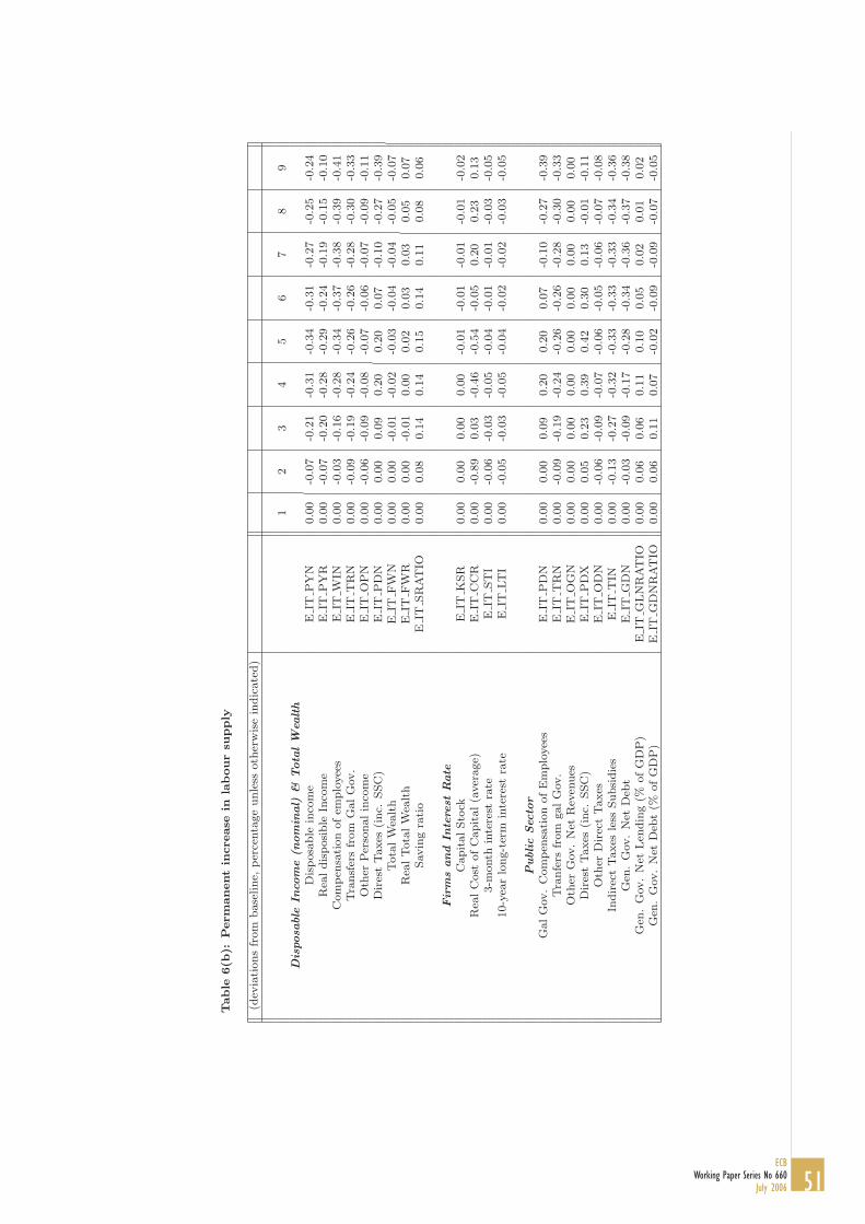
Table

6(b

):Perm

anent

increase

inla

bour

supply

(dev

iati

ons

from

base

line,

per

centa

ge

unle

ssoth

erw

ise

indic

ate

d)

12

34

56

78

9D

isposa

ble

Inco

me

(nom

inal)

&Tota

lW

ealth

Dis

posa

ble

inco

me

EIT

PY

N0.0

0-0

.07

-0.2

1-0

.31

-0.3

4-0

.31

-0.2

7-0

.25

-0.2

4R

ealdis

posi

ble

Inco

me

EIT

PY

R0.0

0-0

.07

-0.2

0-0

.28

-0.2

9-0

.24

-0.1

9-0

.15

-0.1

0C

om

pen

sati

on

ofem

plo

yee

sE

ITW

IN0.0

0-0

.03

-0.1

6-0

.28

-0.3

4-0

.37

-0.3

8-0

.39

-0.4

1Tra

nsf

ers

from

GalG

ov.

EIT

TR

N0.0

0-0

.09

-0.1

9-0

.24

-0.2

6-0

.26

-0.2

8-0

.30

-0.3

3O

ther

Per

sonalin

com

eE

ITO

PN

0.0

0-0

.06

-0.0

9-0

.08

-0.0

7-0

.06

-0.0

7-0

.09

-0.1

1D

ires

tTaxes

(inc.

SSC

)E

ITP

DN

0.0

00.0

00.0

90.2

00.2

00.0

7-0

.10

-0.2

7-0

.39

Tota

lW

ealt

hE

ITFW

N0.0

00.0

0-0

.01

-0.0

2-0

.03

-0.0

4-0

.04

-0.0

5-0

.07

Rea

lTota

lW

ealt

hE

ITFW

R0.0

00.0

0-0

.01

0.0

00.0

20.0

30.0

30.0

50.0

7Savin

gra

tio

EIT

SR

AT

IO0.0

00.0

80.1

40.1

40.1

50.1

40.1

10.0

80.0

6

Fir

ms

and

Inte

rest

Rate

Capit

alSto

ckE

ITK

SR

0.0

00.0

00.0

00.0

0-0

.01

-0.0

1-0

.01

-0.0

1-0

.02

Rea

lC

ost

ofC

apit

al(a

ver

age)

EIT

CC

R0.0

0-0

.89

0.0

3-0

.46

-0.5

4-0

.05

0.2

00.2

30.1

33-m

onth

inte

rest

rate

EIT

ST

I0.0

0-0

.06

-0.0

3-0

.05

-0.0

4-0

.01

-0.0

1-0

.03

-0.0

510-y

ear

long-t

erm

inte

rest

rate

EIT

LT

I0.0

0-0

.05

-0.0

3-0

.05

-0.0

4-0

.02

-0.0

2-0

.03

-0.0

5

Public

Sec

tor

GalG

ov.

Com

pen

sati

on

ofE

mplo

yee

sE

ITP

DN

0.0

00.0

00.0

90.2

00.2

00.0

7-0

.10

-0.2

7-0

.39

Tra

nfe

rsfr

om

galG

ov.

EIT

TR

N0.0

0-0

.09

-0.1

9-0

.24

-0.2

6-0

.26

-0.2

8-0

.30

-0.3

3O

ther

Gov.

Net

Rev

enues

EIT

OG

N0.0

00.0

00.0

00.0

00.0

00.0

00.0

00.0

00.0

0D

ires

tTaxes

(inc.

SSC

)E

ITP

DX

0.0

00.0

50.2

30.3

90.4

20.3

00.1

3-0

.01

-0.1

1O

ther

Dir

ect

Taxes

EIT

OD

N0.0

0-0

.06

-0.0

9-0

.07

-0.0

6-0

.05

-0.0

6-0

.07

-0.0

8In

dir

ect

Taxes

less

Subsi

die

sE

ITT

IN0.0

0-0

.13

-0.2

7-0

.32

-0.3

3-0

.33

-0.3

3-0

.34

-0.3

6G

en.

Gov.

Net

Deb

tE

ITG

DN

0.0

0-0

.03

-0.0

9-0

.17

-0.2

8-0

.34

-0.3

6-0

.37

-0.3

8G

en.

Gov.

Net

Len

din

g(%

ofG

DP

)E

ITG

LN

RAT

IO0.0

00.0

60.0

60.1

10.1

00.0

50.0

20.0

10.0

2G

en.

Gov.

Net

Deb

t(%

ofG

DP

)E

ITG

DN

RAT

IO0.0

00.0

60.1

10.0

7-0

.02

-0.0

9-0

.09

-0.0

7-0

.05

51ECB


5 Conclusions

This paper has documented the structure, estimation and simulation properties ofthe Italian block of the ESCB-multi-country model. This model is used regularly asan input into Eurosystem projection exercises and, to a lesser extent, in simulationanalysis. The model shares similar features with the AWM and the other MCM blocks.After outlining the theoretical and econometric underpinnings of the model, its dynamicand steady-state properties were illustrated using some standard diagnostic simulations.These essentially show the congruence of the model with respect to the exogenousneoclassical growth model. All demand shocks imply an eventual return of outputand the inflation rate to base. However, the components of output (consumption,investment and net trade) depend on relative prices and so may or may not returnto base individually. The adjustment properties of the model, in terms of impactmultipliers for instance, are feasible and trajectories do not appear to be characterizedby excessive volatility or cyclicality. The time profile for reversion to baseline is attime protracted, although this essentially relates to the backward-looking expectationsembodied in the model and ad-hoc adjustment dynamics. Supply side shocks, such asan expansion of the labour force, whilst of course not returning the model trajectoryto some pre-defined base, appear nevertheless reasonable in their properties.

Needless to say, the model (and this class of model) is not without its shortcomings.In this context, we can make four points. First, the absence of model-consistent ex-pectations reduces the model’s realism in capturing the consequences of certain shocks(e.g., permanent, pre-announced ones). Second, the effectively closed-economy natureof the model by definition cuts off feedback from home policies on the rest of the worldand vice versa, one example of which is that the model implies that any level of con-sumption can be financed by external borrowing.7 Third, given its ad-hoc dynamicsand lack of explicit micro-foundations, model properties and shock processes have nostructural interpretation; the model is therefore potentially open to the Lucas Critique.Finally, on a more specific note, the assumption of constant factor income shares (andthus Cobb-Douglas technology) is, whilst extremely common in macro-models, contro-versial for many euro-area countries (and also for Italy) given the well-known downwardtrend in the labour income share since the mid-1970s. One possible remedy, namelyusing a CES production function8, however, involves a significant departure from thestandard MCM framework. We leave treatment of these points open for possible futurework.

References

[1] Angelini, E., F. Boissay, M. Ciccarelli (2006). The Dutch block of the ESCB Multi-Country Model, forth coming ECB WP.

7However, when the model is run in forecast mode, its trade profile is made consistent with intra-and extra- euro area trade flows.

8See the discussion in Klump, McAdam and Willman (2004).


[2] Boissay, F. and J.P. Villetelle (2005). The French block of the ESCB Multi-CountryModel, ECB WP No. 456.

[3] Fagan, G., Henry, J. and R. Mestre (2001). An area-wide model (AWM) for theeuro area, European Central Bank, ECB WP No. 42.

[4] Karlsson, T. and P. McAdam (2005). The EuroSystem’s Multi-Country Model andthe Link Block, in G. Fagan and J. Morgan, J. (Eds.), Econometric Models of theEuro-area Central Banks, Edward Elgar.

[5] Klump, R., P. McAdam and A. Willman (2006). Factor Substitution and FactorAugmenting Technical Progress in the US: A Normalized Supply-Side System Ap-proach, forthcoming in Review of Economics and Statistics. (ECB Working Paper367).

[6] McAdam, P. (1999). The Long Run In Macro Economic Modeling: A Guide, inHughes-Hallett, A J, and P. McAdam, (eds) Analyses In Macro Economic Modeling,Kluwer Academic Press.

[7] Willman, A. and A. Estrada (2002). The Spanish block of the ESCB Multi CountryModel, ECB WP no. 584.

53ECB


6 Appendix A: Names of variables in the Italian MCM

Table 1: Acronyms associated to all variables used in the modelNames DescriptionKRP Capital Stock, private sector (Real)KRW Capital Stock, whole economy (Real)LEX Employees to Employment (Ratio)LEN Total EmployeesLFN Total Labour ForceLGN General government employmentLNN Whole Economy EmploymentLNT Trend EmploymentLSR Outstanding Inventories (Real)LTI Long term interest RateLTR Long term interest Rate (Real)MTD Imports of Goods and Services (Deflator)MTN Imports of Goods and ServicesMTR Imports of Goods and Services (Real)NFA Net foreign AssetsNFN Net Factor IncomeODN Other Direct TaxesOGN Other Govt. Net. RevenueOID Private Gross Domestic Capital Formation (Deflator)OIN Private Gross Domestic Capital FormationOIP Private Gross Domestic Capital Formation Pre-Tax (Deflator)OIR Private Gross Domestic Capital Formation (Real)OLN Other Domestic Net LendingOPN Other Personal IncomeOWN Other sector compensation of employeesOYN Other sector disposable incomePCD Personal Consumer Expenditure (Deflator)PCN Personal Consumer ExpenditurePCP Private Consumption Deflator Pre-Tax (Deflator)PCR Personal Consumer Expenditure (Real)PEI Price/unit value index for imports of energyPOIL Price of Oil in US$PPYB Permanent Income(backward looking) (Real)PROD Productivity per HeadPSN Personal Sector SavingPYN Personal Disposable IncomePYR Personal Disposable Income (Real)RCC Credit interest rate (corporate sector)RCH Credit interest rate (household sector)RMT Mortgage rate (representative)SALE Consumption plus Exports (Real)SCD Change in inventories (Deflator)SCN Change in inventoriesSCR Change in inventories (Real)SGLN Cumulated Current AccountSMC Short-Run Marginal Cost of ProductionSTI Short Term Interest RateSZD Inventories and Stat. Discrepancy (Deflator)SZN Inventories and Stat. DiscrepancyTCI Apparent Tax Rate on ConsumptionTCIR Apparent Tax Rate on Consumption (Rebased)... continue


...TDN Direct Taxes incl. SSCTDNB Tax Base for Direct TaxesTDX Direct Taxes to the Tax Base (Ratio)TGI Apparent Indirect Tax Rate on Government ConsumptionTGIR Apparent Indirect Tax Rate on Government Consumption (Rebased)TII Apparent Indirect Tax Rate on InvestmentTIIR Apparent Indirect Tax Rate on Investment (Rebased)TIN Indirect Taxes less SubsidiesTIR Indirect Taxes less Subsidies (Real)TIX Indirect Taxes less Subsidies (Ratio)TRN Transfers from Gen. GovtTRX Transfers from Gen. Govt (Ratio)TWN Transfers from ROWULA ULC Adjusted (employees)ULC ULCUNN Unemployment (ILO concept)URT Equilibrium Unemployment RateURX Unemployment Rate (ILO concept)WED Foreign Output in Domestic Currency (Deflator)WEN Compensation per EmployeeWER Weighted Import Demand IndicatorWEUD Foreign Output in US$ (Deflator)WIN Compensation to Employees, TotalWUN Compensation to Employees, per HeadWUG Government Compensation, per HeadWUR Real Wage in terms of ConsumptionXTD Exports of Goods and Services (Deflator)XTN Exports of Goods and ServicesXTR Exports of Goods and Services (Real)YED GDP BY EXPENDITURE/INCOME (Deflator)YEN GDP BY EXPENDITURE/INCOMEYER GDP BY EXPENDITURE/INCOME (Real)YFD GDP at Factor Cost (Deflator)YFN GDP at Factor CostYFR GDP at Factor Cost (Real)YFT Potential OutputYGA Output GapYNR Production Using Available Inputs (Real)ZCC1 Stat. Discrep. User Cost of Capital (LTI)ZCC2 Stat. Discrep. User Cost of Capital (RCC)ZED Statistical discrepancy, GDP ExpenditureZEN Statistical discrepancy, GDP ExpenditureZER Statistical discrepancy, GDP ExpenditureZGDN Stat. Discrep. Government Net DebtZGLN Stat. Discrep. Government Net LendingZID Statistical discrepancy, GDP IncomeZIN Statistical discrepancy, GDP IncomeZIR Statistical discrepancy, GDP IncomeZKSR Stat. Discrep. Total Real Capital StockZNFA Stat. Discrep. Net Foreign AssetsZOLN Stat. Discrep. Net Lending Other Private Sector

55ECB


dummy/trend description equationDUMT003 Step dummy from 00q3 onward MTDSTAR

DUMMYQ1DUMMYQ2DUMMYQ3

Seasonal dummies

{∆ log (PEI)∆ log (HEXP )

DUM031 Dummy for 2003q1 ∆ log (IPR)

DUMT951 Step dummy from 95q1 onward GIPSTAR

TIME Trend

KSTARIPRSTARLSTARSCRSTARXTRSTARXTDSTARMTRSTARMTDSTARRWUNSTARPCDSTARHEXPSTAR

TIME2 Quadratic Trend

{YFTLSTARXTRSTARPCDSTAR

For the forecast exercise, all dummies and trends are kept constant over the forecasthorizon. In the simulation exercise, instead, their treatment may be different as longas their effect decays over the future to ensure that all variables grow, in the long run,at their target growth rate.


7 Appendix B: List of dummies and trends

The following dummies and trends have been used in the following equations:

Equations of Italian model POTENTIAL OUTPUT AND OUTPUT GAP it_YFT: it_YFT = exp( + log(it_alpha) + it_beta*log(it_KSR) + (1-it_beta)*log(it_LNN) + (1-it_beta)*(it_gamma*it_TIME) + it_yft.cst + it_yft.time1*it_TIME+ it_yft.time2*it_TIME2)

+res_it_yft, it_YGA: it_YGA = it_YER/it_YFT + res_it_yga, MONETARY POLICY AND INTEREST RATES NOMINAL INTEREST RATES it_STI: it_STI = it_dfor*it_ZZSTI + (1-it_dfor)*(it_taylor*it_STI(-1) + (1-it_taylor)*400*(it_gamma+it_demo+it_infl-1.5*it_infl + 1.5*(it_PCD/it_PCD(-1)-1) + 0.5*(it_YER/it_YER(-1)-1-it_gamma-it_demo)) -(1-it_taylor) )+ res_it_sti, it_LTI: it_LTI = it_dfor*it_ZZLTI + (1-it_dfor)*(it_lti.cst+ it_lti.lt1*it_LTI(-1)+it_lti2*it_LTI(-2)

it_lti.sti*it_STI+ it_lti.sti1*it_STI(-1)+ it_lti.sti2*it_STI(-2) + it_lti.sti3*it_STI(-3)+ it_lti.sti4*it_STI(-4) + it_lti.sti5*it_STI(-5) ) + res_it_lti,

REAL INTEREST RATES it_LTR: it_LTR = 100*((1 + it_LTI/100)/(it_PCD/it_PCD(-4))-1) + res_it_ltr, it_STR: it_STR = 100*((1 + it_STI/100)/(it_PCD/it_PCD(-4))-1) + res_it_str, NOMINAL USER COST OF CAPITAL it_CC0: it_CC0 = it_OID*(it_LTI/400 + it_depkpr - (it_YFD/it_YFD(-4)-1)/4) + res_it_cc0, REAL USER COST OF CAPITAL it_CCR: it_CCR = it_CC0/it_OID + res_it_ccr, FISCAL POLICY AND TAX RATES DEFINITION OF PUBLIC DEBT-TO-GDP RATIO, PERCENT it_GDNRATIO = 100 * it_GDN / (4*it_YEN) , DEFINITION OF PUBLIC DEFICIT-TO-GDP RATIO, PERCENT

57ECB


it_GLNRATIO = 100 * it_GLN / (it_YEN) , DEFINITION OF DEBT TARGET it_DEBT_TARGET = it_debt.target * (IT_YEN/IT_YEN) , it_PDN: it_PDN = it_dfor*it_ZZPDX*it_YEN + (1-it_dfor)* it_PDX * it_PDNB + res_it_pdn, it_PDX: it_PDX = it_fiscrule * ( it_fisc.smooth * it_PDX(-1) + it_fisc.exo * it_PDX + it_fisc.gdn * (it_GDNRATIO - it_DEBT_TARGET)/100 + it_fisc.gln * ( it_GLNRATIO(-1) - it_GLNRATIO(-2) )/100 ) + (1-it_fiscrule)*it_PDX + res_it_PDX, it_ODN: it_ODN = it_dfor*it_ZZODX*it_YEN + (1-it_dfor)*it_ODX*it_ODNB + res_it_odn, it_ODX: it_ODX = it_fiscrule * ( it_fisc.smooth * it_ODX(-1) + it_fisc.exo * it_ODX + it_fisc.gdn * (it_GDNRATIO - it_DEBT_TARGET)/100 + it_fisc.gln * ( it_GLNRATIO(-1) - it_GLNRATIO(-2) )/100 ) + (1-it_fiscrule)*it_ODX + res_it_ODX, PRICE BLOCK DOMESTIC WAGE-PRICE BLOCK it_RWUNSTAR: it_RWUNSTAR = exp( log((1-it_beta)*(it_eps-1)/it_eps) + log(it_YER/it_LNN) + it_rwunstar.cst

+ it_rwunstar.time*it_TIME) , it_WUN: del(log(it_WUN)) = del(log(it_PCD))

it_wun.cst + + it_wun.rwun1*del(log(it_WUN(-1)/it_PCD(-1))) + it_wun.pro*del(log(it_PRO)) + it_wun.urx*(log(it_URX/100)-log(it_nairu)) + it_wun.ecm1*( log(it_WUN(-1)/it_YFD(-1))-log(it_RWUNSTAR(-1)) ) + it_wun.pcyf*del(log(it_PCD/it_YFD)) + res_it_wun, it_YFD: del(log(it_YFD)) = it_yfd.cst + + it_yfd.ecm5*( log(it_YFD(-5)/it_WUN(-5))+log(it_RWUNSTAR(-5)) + it_yfd.yfd1*del(log(it_YFD(-1))) + it_yfd.wun1*del(log(it_WUN(-1))) + it_yfd.wun2*del(log(it_WUN(-2))) + it_yfd.pro1*del(log(it_PRO(-1))) ) + res_it_yfd,


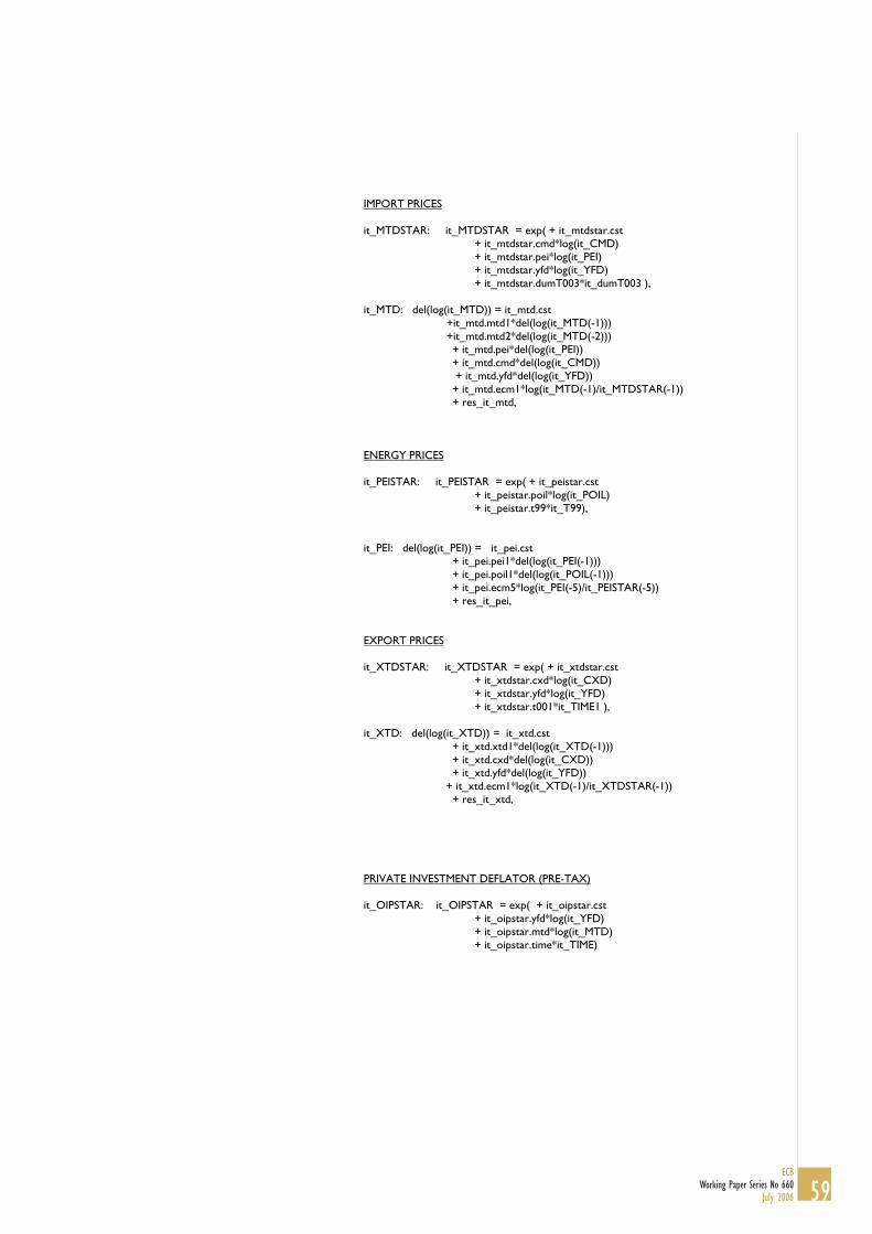
IMPORT PRICES it_MTDSTAR: it_MTDSTAR = exp( + it_mtdstar.cst + it_mtdstar.cmd*log(it_CMD) + it_mtdstar.pei*log(it_PEI) + it_mtdstar.yfd*log(it_YFD) + it_mtdstar.dumT003*it_dumT003 ), it_MTD: del(log(it_MTD)) = it_mtd.cst

+it_mtd.mtd1*del(log(it_MTD(-1))) +it_mtd.mtd2*del(log(it_MTD(-2)))

+ it_mtd.pei*del(log(it_PEI)) + it_mtd.cmd*del(log(it_CMD)) + it_mtd.yfd*del(log(it_YFD)) + it_mtd.ecm1*log(it_MTD(-1)/it_MTDSTAR(-1)) + res_it_mtd, ENERGY PRICES it_PEISTAR: it_PEISTAR = exp( + it_peistar.cst + it_peistar.poil*log(it_POIL) + it_peistar.t99*it_T99), it_PEI: del(log(it_PEI)) = it_pei.cst + it_pei.pei1*del(log(it_PEI(-1))) + it_pei.poil1*del(log(it_POIL(-1))) + it_pei.ecm5*log(it_PEI(-5)/it_PEISTAR(-5)) + res_it_pei, EXPORT PRICES it_XTDSTAR: it_XTDSTAR = exp( + it_xtdstar.cst + it_xtdstar.cxd*log(it_CXD) + it_xtdstar.yfd*log(it_YFD) + it_xtdstar.t001*it_TIME1 ), it_XTD: del(log(it_XTD)) = it_xtd.cst + it_xtd.xtd1*del(log(it_XTD(-1))) + it_xtd.cxd*del(log(it_CXD)) + it_xtd.yfd*del(log(it_YFD)) + it_xtd.ecm1*log(it_XTD(-1)/it_XTDSTAR(-1)) + res_it_xtd, PRIVATE INVESTMENT DEFLATOR (PRE-TAX) it_OIPSTAR: it_OIPSTAR = exp( + it_oipstar.cst + it_oipstar.yfd*log(it_YFD) + it_oipstar.mtd*log(it_MTD) + it_oipstar.time*it_TIME)

59ECB


it_OIP: del(log(it_OIP)) = it_oip.cst + it_oip.oip1* del(log it_OIP(-1)) + it_oip.yfd*del(log(it_YFD)) + it_oip.mtd*del(log(it_MTD)) + it_oip.ecm1*log(it_OIP(-1)/it_OIPSTAR(-1)) + res_it_oip, GOVERNMENT INVESTMENT DEFLATOR (PRE-TAX) it_GIPSTAR: it_GIPSTAR = exp( + it_gipstar.cst + it_gipstar.yfd*log(it_YFD) + it_gipstar.mtd*log(it_MTD) + it_gipstar.dumT951*it_DUMT951), it_GIP: del(log(it_GIP)) = it_gip.cst + it_gip.gip1*del(log(it_GIP(-1))) + it_gip.mtd*del(log(it_MTD)) + it_gip.yfd* del(log(it_YFD)) + it_gip.ecm2*log(it_GIP(-2)/it_GIPSTAR(-2)) + res_it_gip, GOVERNMENT CONSUMPTION DEFLATOR (PRE-TAX) it_GCPSTAR: it_GCPSTAR = exp( + it_gcpstar.cst + it_gcpstar.yfd*log(it_YFD) + it_gcpstar.mtd*log(it_MTD) + it_gcpstar.time*it_TIME ), it_GCP: del(log(it_GCP)) = it_gcp.cst + it_gcp.gcp1*del(log(it_GCP(-1))) + it_gcp.yfd*del(log(it_YFD)) + it_gcp.mtd*del(log(it_MTD)) + it_gcp.ecm4*log(it_GCP(-4)/it_GCPSTAR(-4)) + res_it_gcp, HICP EXCLUDING ENERGY it_HEXPSTAR: it_HEXPSTAR = exp( + it_hexpstar.cst + it_hexpstar.ulc*log(it_WUN/it_PRO) + it_hexpstar.time1*it_TIME1 ), it_HEXP: del(log(it_HEXP)) = it_hexp.cst + it_hexp.hexp2*del(log(it_HEXP(-2))) + it_hexp.yfd2 del(log(it_YFD(-2))) + it_hexp.yfd3 del(log(it_YFD(-3))) + it_hexp.mtd del(log(it_MTD)) + it_hexp.ecm1*log(it_HEXP(-1)/it_HEXPSTAR(-1)) + it_hexp.dumq1*it_DUMMYQ1 + it_hexp.dumq2*it_DUMMYQ2 + it_hexp.dumq3*it_DUMMYQ3 + res_it_hexp,


HICP ENERGY it_HEGSTAR: it_HEGSTAR = exp( + it_hegstar.cst + it_hegstar.yfd*log(it_YFD) + it_hegstar.pei*log(it_PEI) it_HEG: del(log(it_HEG)) = it_heg.cst + it_heg.heg1*del(log(it_HEG(-1))) + it_heg.pei*del(log(it_PEI)) + it_heg.yfd*del(log(it_YFD)) + it_heg.ecm1*log(it_HEG(-1)/it_HEGSTAR(-1)) + res_it_heg, PRIVATE CONSUMPTION DEFLATOR it_PCDSTAR: it_PCDSTAR = exp( + it_pcdstar.cst + it_pcdstar.hic*log(it_HIC) + it_pcdstar.time*it_TIME + it_pcdstar.time2*it_TIME2 it_PCD: del(log(it_PCD) )= it_pcd.cst + it_pcd.ecm1*log(it_PCD(-1)/it_PCDSTAR(-1))

+ it_pcd.pcd1*del(log(it_PCD(-1))) + it_pcd.hic*del(log(it_HIC)) + it_pcd.dumq1*it_DUMMYQ1

+ it_pcd.dumq2*it_DUMMYQ2 + it_pcd.dumq3*it_DUMMYQ3

+res_it_pcd , REAL BLOCK REAL PRIVATE CONSUMPTION it_PCRSTAR: it_PCRSTAR = exp( + it_pcrstar.cst + it_pcrstar.pyr*log(it_PYR) + it_pcrstar.fwr*log(it_FWR) , it_PCR: del(log(it_PCR)) = it_pcr.cst + it_pcr.pcr1*del(log(it_PCR(-1))) + it_pcr.pyr1*del(log(it_PYR(-1))) + it_pcr.urx2*del(log(it_URX(-2)/100)) + it_pcr.ecm1*log(it_PCR(-1)/it_PCRSTAR(-1)) + res_it_pcr,

61ECB


REAL NON-HOUSING PRIVATE INVESTMENT it_KSTAR: it_KSTAR = exp( + log(it_YER) - log(it_alpha) + (1-it_beta)*log(it_WUN/it_YFD) - (1-it_beta)*log(it_CCR) - (1-it_beta)*(it_gamma*it_TIME) + (1-it_beta)*log(it_beta/(1-it_beta)) + it_kstar.cst), it_IPRSTAR: it_IPRSTAR = exp( +log((it_gamma + it_demo+ it_depkpr)/(1+it_gamma+it_demo)) + log(it_YER) - log(it_alpha) + (1-it_beta)*log(it_WUN/it_YFD) - (1-it_beta)*log(it_CCR) - (1-it_beta)*(it_gamma*it_TIME) + (1-it_beta)*log(it_beta/(1-it_beta)) + it_iprstar.cst + it_iprstar.time*it_TIME ), it_IPR: del(log(it_IPR)) = it_ipr.cst + it_ipr.ipr1*del(log(it_IPR(-1))) + it_ipr.ipr2*del(log(it_IPR(-1))) + it_ipr.yer*del(log(it_YER)) + it_ipr.ecm1*log(it_IPR(-1)/it_IPRSTAR(-1)) + res_it_ipr, REAL EXPORTS it_XTRSTAR: it_XTRSTAR = exp( + it_xtrstar.cst + it_xtrstar.wdr*log(it_WDR) + it_xtrstar.xtd*log(it_XTD) + it_xtrstar.cxd*log(it_CXD) + it_xtrstar.time*it_TIME + it_xtrstar.time2*it_TIME2), it_XTR: del(log(it_XTR)) = it_xtr.cst + it_xtr.xtr1*del(log(it_XTR(-1))) + it_xtr.wdr.*del(log(it_WDR)) + it_xtr.een*del(log(it_EEN(-1))) + it_xtr.comp4*del(log(it_XTD(-4)) - log (it_CXD(-4)) ) + it_xtr.ecm1*log(it_XTR(-1)/it_XTRSTAR(-1)) + res_it_xtr,


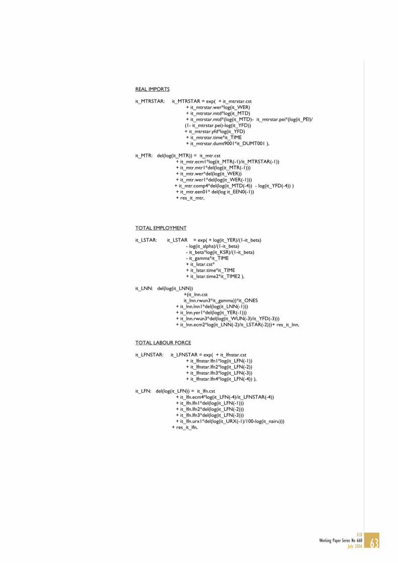
REAL IMPORTS it_MTRSTAR: it_MTRSTAR = exp( + it_mtrstar.cst + it_mtrstar.wer*log(it_WER) + it_mtrstar.mtd*log(it_MTD) + it_mtrstar.mtd*(log(it_MTD)- it_mtrstar.pei*(log(it_PEI)/

(1- it_mtrstar.pei)-log(it_YFD)) + it_mtrstar.yfd*log(it_YFD) + it_mtrstar.time*it_TIME + it_mtrstar.dumt9001*it_DUMT001 ), it_MTR: del(log(it_MTR)) = it_mtr.cst + it_mtr.ecm1*log(it_MTR(-1)/it_MTRSTAR(-1)) + it_mtr.mtr1*del(log(it_MTR(-1))) + it_mtr.wer*del(log(it_WER)) + it_mtr.wer1*del(log(it_WER(-1))) + it_mtr.comp4*del(log(it_MTD(-4)) - log(it_YFD(-4)) ) + it_mtr.een01* del(log it_EEN0(-1)) + res_it_mtr, TOTAL EMPLOYMENT it_LSTAR: it_LSTAR = exp( + log(it_YER)/(1-it_beta) - log(it_alpha)/(1-it_beta) - it_beta*log(it_KSR)/(1-it_beta) - it_gamma*it_TIME + it_lstar.cst* + it_lstar.time*it_TIME + it_lstar.time2*it_TIME2 ), it_LNN: del(log(it_LNN))

+(it_lnn.cst it_lnn.rwun3*it_gamma))*it_ONES

+ it_lnn.lnn1*del(log(it_LNN(-1))) + it_lnn.yer1*del(log(it_YER(-1))) + it_lnn.rwun3*del(log(it_WUN(-3)/it_YFD(-3))) + it_lnn.ecm2*log(it_LNN(-2)/it_LSTAR(-2)))+ res_it_lnn, TOTAL LABOUR FORCE it_LFNSTAR: it_LFNSTAR = exp( + it_lfnstar.cst + it_lfnstar.lfn1*log(it_LFN(-1)) + it_lfnstar.lfn2*log(it_LFN(-2)) + it_lfnstar.lfn3*log(it_LFN(-3)) + it_lfnstar.lfn4*log(it_LFN(-4)) ), it_LFN: del(log(it_LFN)) = it_lfn.cst + it_lfn.ecm4*log(it_LFN(-4)/it_LFNSTAR(-4)) + it_lfn.lfn1*del(log(it_LFN(-1))) + it_lfn.lfn2*del(log(it_LFN(-2))) + it_lfn.lfn3*del(log(it_LFN(-3))) + it_lfn.urx1*del(log(it_URX(-1)/100-log(it_nairu)))

+ res_it_lfn,

63ECB


REAL INVENTORIES it_SCRSTAR: it_SCRSTAR = (it_scrstar.yer+it_scrstar.time1*it_TIME1)*it_YER, it_SCR: del(it_SCR/it_YER) = it_scryer.cst + it_scryer.ecm3*( (it_SCR(-3)-it_SCRSTAR(-3))/it_YER(-31) ) + it_scryer.scryer1*del(it_SCR(-1)/it_YER(-1)) + it_scryer.scryer2*del(it_SCR(-2)/it_YER(-2)) + it_scryer.scryer3*del(it_SCR(-3)/it_YER(-3)) + res_it_scr, ACCOUNTING RELATIONSHIPS it_INFQ: it_INFQ = 100*(it_PCD/it_PCD(-1)-1) + res_it_INFQ, it_INFA: it_INFA = 100*(it_PCD/it_PCD(-4)-1) + res_it_INFA, it_POIL: it_POIL = it_POILU*it_EXR + res_it_poil, it_CMD: it_CMD = it_CMUD * it_EXR + res_it_CMD, it_CXD: it_CXD = it_CXUD * it_EXR + res_it_CXD, it_WDR: it_WDR = it_WDR_in*it_WDR_ex + res_it_WDR, it_CXUD: it_CXUD = it_CXUD_in*it_CXUD_ex + res_it_CXUD, it_CXDIN: it_CXD_IN = it_CXUD_in*(it_EXR**it_betain) + res_it_CXD_IN, it_CXDEX: it_CXD_EX = it_CXUD_ex*(it_EXR**it_betaex) + res_it_CXD_EX, it_CMUD: it_CMUD = it_CMUD_in*it_CMUD_ex + res_it_CMUD, it_CMDIN: it_CMD_IN = it_CMUD_in*(it_EXR**it_m2in) + res_it_CMD_IN, it_CMDEX: it_CMD_EX = it_CMUD_ex*(it_EXR**it_m2ex) + res_it_CMD_EX, it_EEN0: it_EEN0 = it_EEN0_in*it_EEN0_ex + res_it_EEN0, it_EEN: it_EEN = it_EEN_in*it_EEN_ex + res_it_EEN, it_OID: it_OID = it_OIP*(1-it_TIIR)/(1-it_TII) + res_it_oid, it_GCD: it_GCD = it_GCP*(1-it_TGIR)/(1-it_TGI) + res_it_gcd, it_GID: it_GID = it_GIP*(1-it_TIIR)/(1-it_TII) + res_it_gid, it_YED: it_YED = it_YEN/it_YER + res_it_yed, it_ITD: it_ITD = it_ITN/it_ITR + res_it_itd, it_PCP: it_PCD = it_PCP*(1-it_TCIR)/(1-it_TCI) + res_it_pcp, it_HEX: it_HEX = it_HEXP*(1-it_TCIR)/(1-it_TCI) + res_it_hex, it_HIC: it_HIC = it_WE*it_HEG + (1-it_WE)*it_HEX + it_ZHIC + res_it_hic,


it_OIN: it_OIN = it_OID*it_OIR + res_it_oin, it_GIN: it_GIN = it_GID*it_GIR + res_it_gin, it_ITN: it_ITN = it_OIN + it_GIN + res_it_itn, it_PCN: it_PCN = it_PCD*it_PCR + res_it_pcn, it_GCN: it_GCN = it_GCD*it_GCR + res_it_gcn, it_XTN: it_XTN = it_XTD*it_XTR + res_it_xtn, it_MTN: it_MTN = it_MTD*it_MTR + res_it_mtn, it_YFN: it_YFN = it_YFD*it_YFR + res_it_yfn, it_YEN: it_YEN = it_YFN + it_TIN + res_it_yen, it_ITR: it_ITR = it_IHR + it_IPR + it_GIR + res_it_itr, it_OIR: it_OIR = it_IPR + it_IHR + res_it_oir, it_YFR: it_YFR = it_YER - it_TIR + res_it_yfr, it_MKUP: it_MKUP = 100*(1-it_WIN/it_YFN) + res_it_mkup, it_SZD: it_SZD = it_SZN/(it_ZER + it_SCR) + res_it_szd, it_UNN: it_UNN = it_LFN - it_LNN + res_it_unn, it_URX: it_URX = 100*it_UNN/it_LFN + res_it_urx, it_PYR: it_PYR = it_PYN/it_PCD + res_it_pyr, it_KGR: it_KGR = it_GIR + (1-it_depkgr)*it_KGR(-1) + res_it_KGR, it_KPR: it_KPR = it_IPR + (1-it_depkpr)*it_KPR(-1) + res_it_KPR, it_KSR: it_KSR = it_ITR + (1-it_depksr)*it_KSR(-1) + res_it_KSR, it_KHR: it_KHR = it_KSR - it_KPR - it_KGR + res_it_KHR, it_FWN: it_FWN = it_OID*it_KPR(-1) + it_IHD*it_KHR(-1) + it_GDN(-1) + it_NFA(-1) + res_it_fwn, it_FWR: it_FWR = it_FWN/it_PCD + res_it_FWR, it_SALE: it_SALE = it_PCR + it_XTR + it_ITR + res_it_SALE, it_YER: it_YER = it_PCR + it_GCR + it_ITR + it_SCR + it_XTR - it_MTR + it_ZER + res_it_YER, it_SZN: it_SZN = it_YEN - it_PCN - it_GCN - it_ITN - it_XTN + it_MTN + res_it_SZN, it_LEN: it_LEN = it_LEX*it_LNN + res_it_LEN, it_PRO: it_PRO = it_YER / it_LNN + res_it_PRO, it_WIN: it_WIN = it_WUN*it_LNN + res_it_WIN, it_CEX: it_CEX = it_WIN*it_LNN/it_LEN + res_it_CEX,

65ECB


it_ULA: it_ULA = it_WUN/it_PRO + res_it_ula, it_GON: it_GON = it_YEN - it_WIN - it_TIN + it_ZIN + res_it_gon, it_PYN: it_PYN = it_WIN + it_OPN + it_TRN - it_PDN + res_it_pyn, it_PSN: it_PSN = it_PYN - it_PCN + res_it_psn, it_GYN: it_GYN = it_PDN + it_ODN + it_TIN + it_OGN - it_TRN - it_INN + res_it_gyn, it_PDNB: it_PDNB = (1+it_pdnb.win)*it_WIN + it_TRN + it_OPN + res_it_pdnb, it_INN: it_INN = (1/400)*it_STI*it_GDN(-1) + res_it_inn , it_GSN: it_GSN = it_GYN - it_GCN + res_it_gsn, it_GLN: it_GLN = it_GSN - it_GIN + res_it_gln, it_GDN: it_GDN = it_GDN(-1) - it_GLN + it_ZGDN + res_it_gdn, it_ODNB: it_ODNB = it_GON - 0.01*it_ITD*it_KSR(-1) + res_it_odnb, it_OLN: it_OLN = it_CAN - it_PSN - it_GLN + it_IHN + res_it_oln, it_BTN: it_BTN = it_XTN - it_MTN + res_it_btn, it_CAN: it_CAN = it_XTN - it_MTN + it_NFN + it_TWN + it_ZCAN + res_it_can, it_NFN: it_NFN = (1/400)*it_STI*it_NFA(-1) + res_it_nfn, it_NFA: it_NFA = it_NFA(-1) + it_CAN + res_it_nfa, it_OYN: it_OYN = it_GON + it_TWN + it_NFN + it_INN - it_ODN - it_OPN - it_OGN + res_it_oyn, it_PLN: it_PLN = it_PSN - it_IHN + res_it_pln, it_TRN: it_TRN = it_TRX*it_YEN + res_it_trn, it_OPN: it_OPN = it_dfor*it_ZZOPX*it_YEN + (1-it_dfor)*it_OPX*it_GON + res_it_opn, it_WER: it_WER = + it_wer.pcr*it_PCR + it_wer.gcr*it_GCR + it_wer.itr*it_ITR + it_wer.xtr*it_XTR + it_wer.scr*it_SCR + res_it_wer, it_IHN: it_IHN = it_IHR*it_IHD + res_it_ihn, it_TIN: it_TIN = + it_TII*it_OIR*it_OID + it_TII*it_GIR*it_GID + it_TCI*it_PCR*it_PCD + it_TGI*it_GCR*it_GCD + res_it_tin, it_TIR: it_TIR = + it_TIIR*it_OIR + it_TIIR*it_GIR + it_TCIR*it_PCR + it_TGIR*it_GCR + res_it_tir,


67ECB


European Central Bank Working Paper Series

For a complete list of Working Papers published by the ECB, please visit the ECB’s website(http://www.ecb.int)

600 “A speed limit monetary policy rule for the euro area” by L. Stracca, April 2006.

601 “Excess burden and the cost of inefficiency in public services provision” by A. Afonsoand V. Gaspar, April 2006.

602 “Job flow dynamics and firing restrictions: evidence from Europe” by J. Messina and G. Vallanti,April 2006.

603 “Estimating multi-country VAR models” by F. Canova and M. Ciccarelli, April 2006.

604 “A dynamic model of settlement” by T. Koeppl, C. Monnet and T. Temzelides, April 2006.

605 “(Un)Predictability and macroeconomic stability” by A. D’Agostino, D. Giannone and P. Surico,April 2006.

606 “Measuring the importance of the uniform nonsynchronization hypothesis” by D. A. Dias,C. Robalo Marques and J. M. C. Santos Silva, April 2006.

607 “Price setting behaviour in the Netherlands: results of a survey” by M. Hoeberichts andA. Stokman, April 2006.

608 “How does information affect the comovement between interest rates and exchange rates?”by M. Sánchez, April 2006.

609 “The elusive welfare economics of price stability as a monetary policy objective: why NewKeynesian central bankers should validate core inflation” by W. H. Buiter, April 2006.

610 “Real-time model uncertainty in the United States: the Fed from 1996-2003” by R. J. Tetlowand B. Ironside, April 2006.

611 “Monetary policy, determinacy, and learnability in the open economy” by J. Bullardand E. Schaling, April 2006.

612 “Optimal fiscal and monetary policy in a medium-scale macroeconomic model”by S. Schmitt-Grohé and M. Uribe, April 2006.

613 “Welfare-based monetary policy rules in an estimated DSGE model of the US economy”by M. Juillard, P. Karam, D. Laxton and P. Pesenti, April 2006.

614 “Expenditure switching vs. real exchange rate stabilization: competing objectives forexchange rate policy” by M. B. Devereux and C. Engel, April 2006.

615 “Quantitative goals for monetary policy” by A. Fatás, I. Mihov and A. K. Rose, April 2006.

616 “Global financial transmission of monetary policy shocks” by M. Ehrmann and M. Fratzscher,April 2006.

617 “New survey evidence on the pricing behaviour of Luxembourg firms” by P. Lünnemannand T. Y. Mathä, May 2006.


618 “The patterns and determinants of price setting in the Belgian industry” by D. Cornilleand M. Dossche, May 2006.

619 “Cyclical inflation divergence and different labor market institutions in the EMU”by A. Campolmi and E. Faia, May 2006.

620 “Does fiscal policy matter for the trade account? A panel cointegration study” by K. Funkeand C. Nickel, May 2006.

621 “Assessing predetermined expectations in the standard sticky-price model: a Bayesian approach”by P. Welz, May 2006.

622 “Short-term forecasts of euro area real GDP growth: an assessment of real-time performancebased on vintage data” by M. Diron, May 2006.

623 “Human capital, the structure of production, and growth” by A. Ciccone andE. Papaioannou, May 2006.

624 “Foreign reserves management subject to a policy objective” by J. Coche, M. Koivu, K. Nyholmand V. Poikonen, May 2006.

625 “Sectoral explanations of employment in Europe: the role of services” by A. D’Agostino,R. Serafini and M. Ward-Warmedinger, May 2006.

626 “Financial integration, international portfolio choice and the European Monetary Union”by R. A. De Santis and B. Gérard, May 2006.

627 “Euro area banking sector integration: using hierarchical cluster analysis techniques”by C. Kok Sørensen, J. M. Puigvert Gutiérrez, May 2006.

628 “Long-run money demand in the new EU Member States with exchange rate effects”by C. Dreger, H.-E. Reimers and B. Roffia, May 2006.

629 “A market microstructure analysis of foreign exchange intervention” by P. Vitale, May 2006.

630 “Implications of monetary union for catching-up member states” by M. Sánchez, May 2006.

631 “Which news moves the euro area bond market?” by M. Andersson, L. J. Hansen andS. Sebestyén, May 2006.

632 “Does information help recovering structural shocks from past observations?”by D. Giannone and L. Reichlin, May 2006.

633 “Nowcasting GDP and inflation: the real-time informational content of macroeconomic datareleases” by D. Giannone, L. Reichlin and D. H. Small, May 2006.

634 “Expenditure reform in industrialised countries: a case study approach” by S. Hauptmeier,M. Heipertz and L. Schuknecht, May 2006.

635 “Identifying the role of labor markets for monetary policy in an estimated DSGE model”by K. Christoffel, K. Kuester and T. Linzert, June 2006.

636 “Exchange rate stabilization in developed and underdeveloped capital markets”by V. Chmelarova and G. Schnabl, June 2006.

69ECB


637 “Transparency, expectations, and forecasts” by A. Bauer, R. Eisenbeis, D. Waggoner andT. Zha, June 2006.

638 “Detecting and predicting forecast breakdowns” by R. Giacomini and B. Rossi, June 2006.

639 “Optimal monetary policy with uncertainty about financial frictions” by R. Moessner, June 2006.

640 “Employment stickiness in small manufacturing firms” by P. Vermeulen, June 2006.

641 “A factor risk model with reference returns for the US dollar and Japanese yen bond markets”by C. Bernadell, J. Coche and K. Nyholm, June 2006.

642 “Financing constraints and firms’ cash policy in the euro area” by R. Pál and A. Ferrando, June 2006.

643 “Inflation forecast-based-rules and indeterminacy: a puzzle and a resolution” by P. Levine,P. McAdam and J. Pearlman, June 2006.

644 “Adaptive learning, persistence, and optimal monetary policy” by V. Gaspar, F. Smets andD. Vestin, June 2006.

645 “Are internet prices sticky?” by P. Lünnemann and L. Wintr, June 2006.

646 “The Dutch block of the ESCB multi-country model” by E. Angelini, F. Boissay andM. Ciccarelli, June 2006.

647 “The economic effects of exogenous fiscal shocks in Spain: a SVAR approach”by F. de Castro Fernández and P. Hernández de Cos, June 2006.

648 “Firm-specific production factors in a DSGE model with Taylor price setting” by G. de Walque,F. Smets and R. Wouters, June 2006.

649 “Monetary and fiscal policy interactions in a New Keynesian model with capital accumulation andnon-Ricardian consumers” by C. Leith and L. von Thadden, June 2006.

650 “A structural break in the effects of Japanese foreign exchange intervention on yen/dollarexchange rate volatility” by E. Hillebrand and G. Schnabl, June 2006.

651 “On the determinants of external imbalances and net international portfolio flows: a globalperspective” by R. A. De Santis and M. Lührmann, July 2006.

652 “Consumer price adjustment under the microscope: Germany in a period of low inflation”by J. Hoffmann and J.-R. Kurz-Kim, July 2006.

653 “Acquisition versus greenfield: the impact of the mode of foreign bank entry on information andbank lending rates” by S. Claeys and C. Hainz, July 2006.

654 “The German block of the ESCB multi-country model” by I. Vetlov and T. Warmedinger, July 2006.

655

656 “Public debt and long-term interest rates: the case of Germany, Italy and the USA” by P. Paesani,R. Strauch and M. Kremer, July 2006.

“Fiscal and monetary policy in the enlarged European Union” by S. Pogorelec, July 2006.


657 “The impact of ECB monetary policy decisions and communication on the yield curve”by C. Brand, D. Buncic and J. Turunen, July 2006.

658 “The response of firms‘ investment and financing to adverse cash flow shocks: the role of bankrelationships” by C. Fuss and P. Vermeulen, July 2006.

659D. Gerdesmeier and B. Roffia, July 2006.

660 “The Italian block of the ESCB multi-country model” by E. Angelini, A. D’Agostino andP. McAdam, July 2006.

“Monetary policy rules in the pre-EMU era: Is there a common rule?” by M. Eleftheriou,

ISSN 1561081-0

9 7 7 1 5 6 1 0 8 1 0 0 5

Documents

The Italian block of the ESCB multi-country model Elena Angelini, Antonello D‘Agostino ISSN 1561081-0 9 771561 081005 WORKING PAPER SERIES NO 660 / JULY 2006 THE ITALIAN BLOCK OF