The economic effects of exogenous fiscal shocks in Spain ... · issn 1561081-0 9 771561 081005 working paper series no 647 / june 2006 the economic effects of exogenous fiscal shocks

ISSN 1561081-0

9 7 7 1 5 6 1 0 8 1 0 0 5

WORKING PAPER SER IESNO 647 / JUNE 2006

THE ECONOMIC EFFECTS OF EXOGENOUS FISCAL SHOCKS IN SPAIN

A SVAR APPROACH

and Pablo Hernández de Cosby Francisco de Castro Fernández

In 2006 all ECB publications will feature

a motif taken from the

€5 banknote.

WORK ING PAPER SER IE SNO 647 / JUNE 2006

This paper can be downloaded without charge from http://www.ecb.int or from the Social Science Research Network

electronic library at http://ssrn.com/abstract_id=901582

1 The authors would like to thank L. J. Álvarez, I. Argimón, A. L. Gómez, J. F. Jimeno, P. L’Hotellerie, E. Ortega, the participants at the Seminar at the Bank of Spain and an anonymous referee for their useful comments and suggestions. The opinions and views

expressed in this paper do not necessarily reflect those of the Bank of Spain or the ECB.

3 European Central Bank, Kaiserstrasse 29, 60311 Frankfurt am Main, Germany; e-mail: [email protected]

THE ECONOMIC EFFECTS OF

EXOGENOUS FISCAL SHOCKS IN SPAIN

A SVAR APPROACH 1

by Francisco de Castro Fernándezand Pablo Hernández de Cos

2 Research Department, Bank of Spain, C/Alcalá 48, E-28014 Madrid, Spain; e-mail: [email protected]

© European Central Bank, 2006

AddressKaiserstrasse 2960311 Frankfurt am Main, Germany

Postal addressPostfach 16 03 1960066 Frankfurt am Main, Germany

Telephone+49 69 1344 0

Internethttp://www.ecb.int

Fax+49 69 1344 6000

Telex411 144 ecb d

All rights reserved.

Any reproduction, publication andreprint in the form of a differentpublication, whether printed orproduced electronically, in whole or inpart, is permitted only with the explicitwritten authorisation of the ECB or theauthor(s).

The views expressed in this paper do notnecessarily reflect those of the EuropeanCentral Bank.

The statement of purpose for the ECBWorking Paper Series is available fromthe ECB website, http://www.ecb.int.

ISSN 1561-0810 (print)ISSN 1725-2806 (online)

3ECB

Working Paper Series No 647June 2006

CONTENTS

Abstract 4

Non-technical abstract 51 Introduction 7

2 Methodological issues 9

2.1 The VAR specification 9

2.2 Identification of fiscal policy shocks 11

3 The effects of government expenditure shocks 17

3.1 The baseline specification 17

3.2 The effects of different publicexpenditure components 20

4 The effects of net taxes 21

4.1 The baseline specification 21

4.2 The effects of different net-taxcomponents 23

5 Robustness checks 24

6 An application to the analysis of the contributionof discretionary fiscal policy to GDPgrowth since the mid-nineties 27

7 Conclusions 30

Appendix A: Construction of output and priceelasticities 33

References 36

Tables and figures 40

European Central Bank Working Paper Series 51

Abstract:

This paper estimates the effects of exogenous fiscal policy shocks in Spain

in a VAR framework. Government expenditure expansionary shocks are

found to have positive effects on output in the short-term at the cost of

higher inflation and public deficits and lower output in the medium and long

term. Tax increases are found to drag economic activity in the medium term

while entailing an only temporary improvement of the public budget

balance. The application of these results to the analysis of fiscal policy in

Spain since the mid-nineties points to the conclusion that the consolidation

process does not seem to have involved costs in terms of output growth.

Moreover, the stance of fiscal policy has become more counter-cyclical in

that period.

JEL Classification no.: E62, H30

Keywords: VAR; Fiscal Shocks; Fiscal multipliers.

4ECBWorking Paper Series No 647June 2006

The role of fiscal policy in influencing economic activity has been one of

the most extensively discussed issues by both academics and policy-makers.

A renewed emphasis on this issue has recently been observed in the

European Monetary Union (EMU), where fiscal policy emerges as the only

instrument on the demand side in the hands of Member States to offset

idiosyncratic shocks.

Despite this relevance, the empirical evidence does not provide a

common picture. In particular, although most of the recent literature shows

positive short-term output multipliers stemming from public expenditure

is very disperse. There is even some evidence of negative fiscal multipliers

for some OECD countries in the post-1980 period, and a recent stream of

the literature has found positive output responses following fiscal

retrenchments, under certain circumstances.

Against this background, this paper aims at providing evidence for the

case of Spain on the effects of fiscal policy shocks on a set of key

macroeconomic variables. Our results show that increases in government

expenditure have a positive impact on economic growth in the short term,

while the effect turns negative in the longer term. Moreover, net-tax

5ECB


increases and tax cuts, the estimated magnitude and duration of these effects

Non-technical Abstract

increases produce negative responses on output in the medium term. As

regards the effect on prices, government expenditure shocks yield

significant effects on prices of the same sign, and net-tax increases yield

negative short-term price responses. Both government expenditure and net-

tax increases generate public deficits in the medium term. Finally, the

responses of GDP or prices are found to differ significantly depending on

the spending or tax component considered.

Two main policy conclusions could be drawn from these results. Firstly,

fiscal policy is able to stimulate economic activity through expenditure

expansions at the cost of higher inflation and public deficits and lower

output in the medium term. In this respect, the fiscal policy implemented in

Spain since the mid-nineties seems to have contributed to create, from a

medium-term perspective, better conditions for economic growth, and the

consolidation process applied in this period does not seem to have involved

significant costs in terms of output growth. Furthermore, the stance of fiscal

policy has also become more counter-cyclical since the late nineties.

Secondly, attempts to achieve fiscal consolidation by increasing the tax

burden might fail to succeed and, given the dynamic interrelations between

public revenues and expenditure, are likely to involve even higher deficits in

the future. Last, but not least, such a policy might slow economic activity

down in the medium term.


1

The role of fiscal policy in influencing economic activity has been one of

the most extensively discussed issues by both academics and policy-makers.

A renewed emphasis on this issue has recently been observed in the

European Monetary Union (EMU), where fiscal policy emerges as the only

instrument on the demand side in the hands of Member States to offset

idiosyncratic shocks.

Despite this relevance, we know surprisingly very little about the effects

of fiscal policy on economic activity (Perotti, 2001). From a theoretical

point of view, the sign and magnitude of the impact of discretionary fiscal

policy on aggregate demand depend on a number of key assumptions1, with

different models offering often opposite conclusions.

The empirical evidence does not provide a common picture either. In

particular, although most of the recent literature, based either on structural

macro models or on VAR analysis, shows positive short-term output

multipliers stemming from public expenditure increases and tax cuts, the

estimated magnitude and duration of these effects is very disperse (see

Table 1 for a brief summary of the effects of fiscal policy shocks on GDP

and prices in selected VAR studies). There is even some evidence of

1 Including, inter alia, the existence of nominal rigidities in the economy, the elasticity of the labour supply, the interest-rate elasticity of investment, the interest-rate and income elasticities of money demand, the degree of openness of the economy, the exchange-rate

7ECB


Introduction

negative fiscal multipliers for some OECD countries in the post-1980 period

(Perotti, 2004). In addition, a recent stream of the literature that aims at

explaining the economic effects of fiscal consolidations has found, under

certain circumstances, positive output responses following fiscal

retrenchments, the so-called non-Keynesian effects of fiscal policy

(Giavazzi and Pagano, 1990; European Commission, 2003; Perotti, 1999)2.

Against this background, this paper aims at providing evidence for the

case of Spain on the effects of exogenous fiscal policy shocks on a set of

key macroeconomic variables within a VAR framework. Most of the recent

existing evidence on the responses to fiscal policy shocks relies indeed on

SVAR models, with the main differences among papers coming from the

alternative approaches followed to identify the fiscal policy shocks. These

approaches can be summarised in four (Perotti, 2004): (1) identification of

fiscal policy shocks by using dummy variables that capture specific

episodes such as the military build-ups corresponding to the Korean and the

Vietnam wars or the Reagan fiscal expansion in the case of the US

(Burnside et al., 1999; Ramey and Shapiro, 1998; Edelberg et al., 1998); (2)

imposition of sign restrictions on the impulse-response functions

(Mountford and Uhlig, 2002); (3) identification of fiscal shocks based on a

regime, the magnitude of the wealth effects, the presence of forward-looking agents and, more generally, the role played by rational expectations. 2 See also Giudice et al. (2003) for a synthesis of the theoretical arguments behind the non-Keynesian effects along with a useful compilation of the relevant empirical evidence.


Choleski ordering (Favero, 2002; Fatás and Mihov, 2001); (4) and finally,

identification of fiscal policy shocks by exploiting decision lags in policy

making and information about the elasticity of fiscal variables to economic

activity (Blanchard and Perotti, 2002; Perotti, 2004). This latter approach is

the one we follow in this paper. In this respect, our results add to the

previous evidence on the same topic already available for Spain obtained

with alternative identification schemes (De Castro, 2005; Marcellino, 2002).

The rest of the paper is organised as follows: section 2 describes the data

and addresses the methodological issues related to the specification and

identification of the VAR; section 3 presents the results stemming from

expenditure shocks, whereas section 4 focuses on the effects of shocks to

net taxes; section 5 analyses the robustness of the results, section 6 includes

an application of our results to the analysis of the contribution of fiscal

policy to GDP growth in Spain since the mid-nineties and, finally, section 7

concludes.

2 Methodological issues

2.1 The VAR specification

Our benchmark specification of the VAR includes quarterly data on public

expenditure (gt), net taxes (tt) and GDP (yt) in real terms3, the GDP deflator

3 In all cases the GDP deflator is employed so as to obtain the corresponding real values.

9ECB


(pt) and the three-year interest rate of government bonds (rt)4. gt is defined

as the sum of public consumption5 and public investment, whereas tt

includes public revenues net of transfers6, excluding interest payments on

government debt. Thus the general government primary budget balance is

obtained as the difference between the levels of tt and gt. All variables are

seasonally adjusted and enter in logs except the interest rate, which enters in

levels. The sample covers the period 1980:1-2004:47.

The reduced-form VAR can be written as

ttt UXLDX += −1)( (1)

where Xt ≡ (gt, tt, yt, pt, rt) is the vector of endogenous variables. The only

deterministic component is a constant term and D(L) is an autoregressive lag

polynomial. The vector Ut ≡ ( rt

pt

yt

tt

gt uuuuu , , , , ) contains the reduced-form

residuals, which in general will have non-zero correlations. Model (1) is

estimated by OLS and the number of lags was set to five according to the

information provided by LR tests and the Akaike information criterion.

4 The inclusion of the long-term interest rate instead of the short-term one is justified for its closer relationship with consumption and investment decisions. 5 Compensation of civil servants plus other consumption expenditure items such as purchases of goods and services. 6 It includes both current and capital transfers. More concretely, transfers include all expenditure items except public consumption, public investment and interest payments. 7 GDP volumes and deflator have been taken from the Quarterly National Accounts (National Institute of Statistics, INE) while the three-year bond rate has been obtained from the Banco de España database. The quarterly fiscal variables were taken from Estrada et al. (2004), which were estimated applying monthly and quarterly official fiscal indicators on a cash basis to the official ESA-95 annual account data.


In order to account for the effects on private consumption and investment,

two alternative 6-variable VAR models were used. They included the

original five variables of the baseline specification plus one of both private

sector variables.

2.2 Identification of fiscal policy shocks

The reduced-form residuals have little economic significance in that they

are linear combinations of structural shocks. In particular, following

Blanchard and Perotti (2002) and Perotti (2004), the reduced-form residuals

of the gt and tt equations, gtu and t

tu , can be thought of as linear

combinations of three types of shocks: a) The automatic responses of

spending and net taxes to GDP, price and interest rate innovations, b)

systematic discretionary responses of fiscal policy to the macro variables in

the system, and c) random discretionary fiscal policy shocks, taken as the

truly uncorrelated structural fiscal policy shocks. Thus, the reduced-form

residuals in the first two equations can be decomposed as:

gt

tttg

rtrg

ptpg

ytyg

gt eeuuuu ++++= ,,,, βααα (2a)

tt

gtgt

rtrt

ptpt

ytyt

tt eeuuuu ++++= ,,,, βααα (2b)

11ECB


where ( gte , t

te ) are the structural orthogonal shocks of government

expenditure and net taxes8, respectively.

In particular, we are interested in analysing the effects of the structural

discretionary fiscal shocks, gte and t

te , on the rest of the variables of the

system, for which estimations for the αi,j’s and βi,j’s in (2) are needed. The

use of quarterly variables allows for setting the discretionary

contemporaneous response of government expenditure or net taxes to GDP,

prices or interest rate innovations to zero in that it typically takes longer

than three months to approve and implement new measures. Therefore, the

coefficients αi,j’s in (2a) and (2b) only reflect the automatic responses of

fiscal variables to innovations in the rest of the variables of the system, the

first component mentioned above.

Given that interest payments on government debt are excluded from the

definitions of expenditure and net taxes, the semi-elasticities of these two

fiscal variables to interest rate innovations, i.e. αg,r and αt,r, were set to zero.

While this assumption appears justified for government expenditure and

plays no role when analysing its effects, it is slightly more controversial for

net taxes9.

8 Similarly, y

te , pte , r

te would be the structural orthogonal shocks derived from the reduced-form residuals in the other three equations related to activity, prices and interest rate, respectively. 9 The income tax-base includes interest income as well as dividends, which covary negatively with interest rates. Nevertheless, the full set of effects of interest rate innovations


Consider now equation (2a). Our choice of the items included in the

definition of government expenditure, notably public consumption and

investment, makes it hard to think about any automatic response of public

expenditure to economic activity. Accordingly, we can set αg,y= 0. The case

of the price elasticity is different, though. Some share of purchases of goods

and services are likely to respond to the price level. In addition, the wage

component is typically indexed to the CPI, even though indexation takes

place with some delay. Thus, an eclectic approach was adopted and,

following Perotti (2004) the price elasticity of government expenditure was

set to -0.5. The relevance of this choice, however, seems very limited in

that, as it will be explained ahead, setting this price elasticity to zero does

not seem to affect the results significantly.

As for (2b), the output and price elasticities αi,j are weighted averages of

the elasticities of the different net-tax components, including transfers,

computed on the basis of information like statutory tax rates and estimations

of the contemporaneous response of the different tax-bases and, in the case

of transfers, the relevant macroeconomic aggregate to GDP and price

changes. In general, the contemporaneous output elasticity of net taxes can

be calculated as:

on the different tax categories are very complex to analyse and, on the other hand, their contemporaneous effects are deemed to be very small.

13ECB


TTi

yBi

BTyt iii ,,, εεα ∑= (3)

with ∑= iTT being the level of net taxes10, ii BT ,ε the elasticity of the ith

category of net taxes to its own tax base and yBi ,ε the GDP elasticity of the

tax base of the ith category of net taxes. The price elasticities for some

components of net taxes were, however, obtained directly through

econometric estimation, whereas others were calibrated. Appendix A

explains in detail the procedure followed to obtain such elasticities.

Once the output and price elasticities have been estimated, the so-called

“adjusted” fiscal shocks (uCA) can be derived as follows:

gt

tttg

rtrg

ptpg

ytyg

gt

CAgt eeuuuuu +=++−= ,,,,

, )( βααα (3a)

tt

gtgt

rtrt

ptpt

ytyt

tt

CAtt eeuuuuu +=++−= ,,,,, )( βααα (3b)

Some further assumptions are needed here and they depend on our view

of the functioning of fiscal policy. If one believes that expenditure decisions

are prior to tax ones, βg,t would be zero. Hence, gte could be recovered

directly from (3a) and use it in (3b) so as to estimate βt,g by OLS.

Conversely, if tax decisions are deemed to come first, we would have to

proceed symmetrically so as to get an estimate of βg,t. It could be quite

difficult to find arguments that fully justify any of both orderings.

Therefore, we decided to present our results on the basis that expenditure


comes first, i.e. βg,t = 0. Nevertheless, this choice does not seem to affect the

main results in a substantial way11, as it will be shown later on.

Since we are interested in studying the effects of fiscal policy shocks, the

ordering of the remaining variables is immaterial to the results.

Accordingly, the reduced-form output residuals are assumed to be a linear

combination of the fiscal shocks.

yt

ttty

gtgy

yt euuu ++= ,, γγ (4)

By definition, some contemporaneous correlation between the reduced-

form residuals of the fiscal equations and yte is expected. Hence (4) is

estimated by instrumental variables, using the structural uncorrelated fiscal

shocks gte and t

te as instruments for gtu and t

tu . Likewise, the price

equation

pt

ytyp

tttp

gtgp

pt euuuu +++= ,,, γγγ (5)

can be estimated by using gte , t

te and yte as instruments. And finally, the

interest rate equation

rt

ptpr

ytyr

tttr

gtgr

rt euuuuu ++++= ,,,, γγγγ (6)

can be estimated accordingly once pte has been recovered.

As a result, the innovation model can be written as

10 The Ti’s are positive in the case of taxes and negative in the case of transfers. 11 In fact, this is mainly due to the low and non-significant correlation between expenditure and net-tax shocks.

15ECB


tt VU Β=Γ (7)

where Vt is the vector containing the orthogonal structural shocks,

⎟⎟⎟⎟⎟⎟

⎠

⎞

⎜⎜⎜⎜⎜⎜

⎝

⎛

−−−−−−−

−−−−−−−−

=Γ

101001

1001

,,,,

,,,

,,

,,,

,,,

pryrtrgr

yptpgp

tygy

rtptyt

rgpgyg

γγγγγγγ

γγαααααα

(8)

and

⎟⎟⎟⎟⎟⎟

⎠

⎞

⎜⎜⎜⎜⎜⎜

⎝

⎛

=Β

10000010000010000010001

,

,

gt

tg

ββ

(9)

Accordingly, the reduced-form residuals are linear combinations of the

orthogonal structural shocks of the form:

tt VU ΒΓ= −1 (10)

Table 2 shows the estimated coefficients for the baseline model. All of

them have the expected sign except γr,y, that yielded a negative value. Given

that it turned out to be non-significant, it was decided to fix it to zero.

Finally, we are also interested in characterising the responses of some

GDP components such as private consumption and private investment, for

which these variables are added in turn to the VAR. The identification of the

resulting 6-variable VARs was achieved by departing from (8) and (9) and


estimating the contemporaneous bi-directional interaction between GDP and

its respective component12.

3 The effects of government expenditure shocks

3.1 The baseline specification

Figure 1 displays the responses of the endogenous variables to a positive

expenditure shock13. It should be first highlighted that the expenditure shock

turns out to be very persistent and only becomes insignificant after almost

five years. The high persistence of public expenditure shocks is in line with

the existing evidence for other OECD countries (Perotti, 2004; Galí et al.,

2003).

The increase of government expenditure raises GDP, which peaks in the

3rd quarter after the shock. The cumulative output multipliers14 are slightly

above one in the first two years: 1.31 and 1.33 in the fourth and eight

quarters after the shock, respectively (see Table 3). These multipliers are

broadly in line with previous studies for the case of Spain (De Castro,

2005), although they are on the high side compared with the values obtained

12 Another possibility would be to replace GDP by one of both components and re-estimate Γ accordingly. However, both approaches yield very similar results. 13 The responses of private consumption and private investment obtained from a 6-variable VAR are also depicted. In all cases, impulse responses are reported for ten years and the one-standard deviation confidence bands have been obtained by Monte Carlo integration methods with 500 replications. 14 The cumulative dynamic multiplier at a given quarter is obtained as the ratio of the cumulative response of GDP and the cumulative response of government expenditure.

17ECB


for other OECD countries (Fatás and Mihov, 2001; Mountford and Uhlig,

2002; Perotti, 2004; Galí et al., 2003). The sign and magnitude of these

VAR short-term responses are also consistent with the short-term

multipliers obtained with macroeconometric models. In particular, Estrada

et al. (2004) report output multipliers of government spending in Spain of

1.2 at the end of the first year and 1.4 after eight quarters.

In the longer term, however, our results show that the GDP response

dwindles steadily and becomes significantly negative after four years. This

evidence is also in line with the negative medium-term output responses

obtained for some other OECD countries (Perotti, 2004; Neri, 2001;

Mountford and Uhlig, 2002).

As regards the impact on other fiscal variables, net-tax revenues rise and

remain positive and significant for approximately twelve quarters, turning

negative in the medium term, following the decline in economic activity.

The initially positive response of net-tax collections offsets the increase of

public expenditure in the quarters following the shock. In the medium term,

however, a persistent deterioration in the primary balance shows up as

expected.

Higher government expenditure also brings about a persistent positive

response of the GDP deflator, which implies higher inflation in the quarters

following the shock. This is a potentially important result since, although De


Castro (2005) already obtains evidence of this kind for Spain, this is far

from being a general finding in VAR analysis. In fact, the evidence from

this literature on the effects of government spending shocks on prices or

inflation is rather mixed15. Our results are, in any case, consistent with those

derived from macromodels for Spain, which find relatively large positive

effects on inflation stemming from government expenditure shocks (Estrada

et al., 2004; Henry et al., 2004).

Likewise, interest rates increase persistently following a positive shock to

government expenditure16. While the positive response of the interest rate

in the short term might be due to higher demand and inflationary pressures,

the persistent deterioration of the primary balance could contribute to

sustain the interest rate above its baseline values. Moreover, the real interest

rate17 rises. Such increase is significant on average over the first three years

after the shock, thereby helping to drag economic activity.

15 For the US, Fatás and Mihov (2001) and Mountford and Uhlig (2002) show negative effects on prices after a positive government spending shock, while Perotti (2004) finds an initial positive impact and negative effects thereafter on the CPI over the period 1961-2000; for the sub-period starting in 1980, the effects (albeit not significant) are instead positive after one, twelve and twenty quarters and negative after four quarters. Edelberg et al. (1998) find a negative effect after an initial positive effect, Neri (2001) reports no significant effects and Canzoneri et al. (2002) find a temporary rise in inflation after a brief decline. For other OECD countries, Perotti (2004) finds positive effects of government spending on prices in Germany, the UK and Australia, and negative, albeit small, in Canada. Marcellino (2002) reports minor and not statistically significant effects on inflation in Germany, Italy and Spain and a positive and significant effect in France in the short term. For a summary of all these results see Henry et al. (2004). 16 In contrast, Perotti (2004) finds no clear-cut evidence in either direction on this issue. 17 The real interest rate is obtained as the difference between the nominal interest rate and the observed annual inflation rate in the same period. We are aware that this definition may be controversial from a theoretical point of view in that it implicitly assumes that expected

19ECB


As for the GDP components, the augmented VAR yields patterns of

response for private consumption and investment quite similar to that of

GDP, going up in the quarters following the shock and declining in the

longer term. Thus, private consumption reaches its peak in the 5th quarter,

whereas private investment peaks somewhat earlier. These short-run effects

are again consistent with those derived from macro models for Spain and, as

regards consumption, with most of the VAR evidence for other countries

(Fatás and Mihov, 2001; Blanchard and Perotti, 2002; Gali et al., 2003). The

evidence for private investment is however more mixed, with some papers

showing negative responses of this variable to an exogenous increase in

government spending.

3.2 The effects of different public expenditure components

In order to account for the different effects on economic activity stemming

from public consumption expenditure and public investment, aggregate

expenditure is replaced in the VAR by either component in turn in both the

baseline and augmented VARs. Figure 2 shows the corresponding impulse

response functions.

Neither public consumption nor investment shocks appear too persistent.

In both cases, GDP increases and peaks in the third quarter. The GDP

inflation equals observed inflation. Nevertheless, we consider that it can represent an


response to a public consumption shock becomes significantly negative

from the fourth quarter onwards. This fall is also observed in the responses

of private consumption and investment, which reproduce output movements

quite closely. Interestingly, Figure 2 shows that main culprit for the GDP

decline is the wage bill component of public consumption18.

In contrast, the positive response of GDP to public investment shocks is

of significantly lower magnitude19, although it takes more time, around

eight quarters, to fade away. Thereafter, the GDP response becomes non-

significant. In the same vein, private consumption and investment show

positive responses in the first two years after the shock.

Finally, all expenditure items entail positive short-term price responses.

However, in the case of increases in the wage bill, this positive response

fades away quickly as a result of the negative effects on economic activity.

4 The effects of net taxes

4.1 The baseline specification

Figure 3 shows the responses following an increase of net taxes. Around

70% of the initial shock disappears after four quarters, although the

acceptable approximation. 18 These results are consistent with the hypothesis that public wage increases may exert upward pressure on the equilibrium wage, leading to lower profits and investment (Alesina et al., 2002).

21ECB


response remains significant until the end of the third year. Higher revenues

encourage government spending, which increases significantly after 2

quarters and remains significant for four years. Such an increase in

government expenditure is high enough to eventually offset the rise in net

taxes, for which the initial improvement of the primary budget balance

phases out over three years and deteriorates thereafter. Thus, on a cumulated

basis, the primary balance rises until the 12th quarter or so and fades

thereafter.

This deterioration of the public deficit in the long term following an

increase in taxes is in accordance with previous evidence on the existence of

a bias towards deficit in public sector’s size in Spain. In addition, the

significant responses of either fiscal variable after shocks to the other one

are also compatible with the existing empirical evidence of bi-directional

causality between public revenues and expenditure (De Castro et al., 2004).

The GDP response to the tax shock, although positive due to the parallel

increase of government expenditure, is largely non-significant in the first

years after the shock. Expectedly, however, the response becomes negative

in the medium term20. As in the case of expenditure shocks, net-tax shocks

19 Nevertheless, the correct way to address the ability of stimulating economic activity is by means of output, consumption and investment multipliers, since the size of the response by itself is little informative. 20 The international evidence on this issue is mixed. Mountford and Uhlig (2002), Marcellino (2002) and Canzoneri et al. (2002) find no significant results, while Neri (2001) shows negative effects on output following a positive tax shock. Furthermore, the sign and


yield positive and persistent effects on nominal and real interest rates. In this

respect, the persistently higher interest rates might be helping to amplify the

negative effects on activity derived from higher taxes.

As far as GDP components are concerned, private consumption and

investment responses, in general, mimic the GDP’s one. Some slight

differences can be observed, though, especially in the short-term behaviour.

Specifically, while private consumption rises in the short term, the response

of private investment is non significant. Despite this initial difference, clear

negative responses in the medium term arise in both cases.

Finally, prices fall in the first 8 quarters after the tax shock and become

non-significant thereafter21.

4.2 The effects of different net-tax components

As in the case of government expenditure items, net-tax components are

found to have different effects on economic variables (see Figure 4). In sum,

size of output responses in Perotti (2004) varies widely depending on the country and period considered. For instance, in the post-1980 period he obtains positive short-term output responses to net-tax shocks too. 21 The international evidence on this effect is again rather mixed, Mountford and Uhlig (2002) find that a net-revenue shock has a negligible effect on prices in the US when controlling for the business cycle and for monetary policy shocks, while in Canzoneri et al. (2002) the inflation response to a net-tax increase is negative, although very small, after an initial minor positive effect. Marcellino (2002) reports non-significant effects on inflation of positive tax shocks in France, Germany and Spain, while inflation significantly increases in Italy in the short run. Perotti (2004) finds that, especially in the post-1980 period, the impact of a tax shock on prices is very small, typically negative or zero, while after three years there is evidence of a positive effect in UK and Australia, although only in the latter is the effect sizeable.

23ECB


shocks to indirect taxation seem to involve no clear effects on economic

activity, whereas shocks to direct taxation are clearly contractionary in the

medium term22. Moreover, shocks to social security contributions also drag

economic activity in the short term23.

As for the effects on prices, increases of indirect taxes involve, as

expected, positive price responses, whereas shocks to direct taxes do not

appear to have significant effects. These two results seem to fit well with the

existing evidence provided by simulations with macromodels (Henry et al.,

2004). Prices fall, however, in response to a shock to social security

contributions, which seems to be explained by the subdued economic

activity in the first quarters following the shock.

5 Robustness checks

In order to test to what extent the results presented above are conditioned by

the assumptions made on some coefficients in matrixes Γ and Β defined in

section 2 some alternative specifications were tried. The first one has to do

with possibly the most controversial assumption in the identification

process: the ordering of fiscal variables. As pointed out before, it is difficult

22 This result is rather intuitive and differs from De Castro (2005). In this respect, the identification scheme adopted here appears more accurate in order to account for the effects of net taxes and, in particular, their breakdown. 23 According to the responses in Figure 4, shocks to social security contributions yield positive output effects after five years, which turns out to be rather counter-intuitive.


to justify that expenditure decisions are prior to tax ones or the opposite. In

this regard, De Castro et al. (2004) show that, depending on the period

under scrutiny, the direction of causality between revenues and expenditure

in Spain varies. Accordingly, we decided to re-estimate under the alternative

assumption that taxes come first, which implies imposing βt,g = 0 and

estimate βg,t in (3.a) by OLS.

Since the reduced-form residuals in the expenditure and net-tax equations

showed low and non-significant correlation, the differences with the

baseline VAR results, if any, were minimal. As a matter of fact, none of the

variables under analysis showed different response profiles and the output

multipliers were almost identical.

Setting the price elasticity of government expenditure exogenously, in our

case αg,p = -0.5, may appear controversial too. In order to have an idea of the

sensitivity of our results to this assumption, an alternative specification

setting αg,p = 0.0 was run. As in the former case, our results appear quite

robust to different parameterisations in that no significant differences were

perceived with respect to the benchmark specification.

Furthermore, we were interested in checking the sensitivity of our results

to different output and price elasticities of net taxes. Firstly, we run the

model setting εt,y = 0.4 exogenously. Secondly, a similar exercise was

However, the forecasting limitations of this methodology for such long horizons advise

25ECB


carried out with εt,y = 0.4 jointly with εt,p = 0.5, instead of the estimated 0.78

in the baseline VAR. In both cases the results were almost identical to the

baseline specification and the output multipliers of government expenditure

were exactly the same as those reported in the first row of Table 3.

The baseline specification was also estimated with detrended variables,

for which Hodrick-Prescott trends were used (with λ=1600). Although in

this case the numbers change, the main conclusions remain valid. In

particular, expenditure shocks lead to higher prices, interest rates and net

taxes. Moreover, GDP always increases in the short term and tends to

decline after some quarters. Furthermore, following a net-tax shock, prices

fall, expenditure rises and output increases in the short term and declines in

the medium term.

Finally, in order to check the stability of our results by sub-samples, we

re-estimated the model for the period between 1992:1 and 2004:4. With this

sub-sample the estimated discretionary fiscal shocks seem to have been less

persistent, with real effects of significantly lower magnitude and largely

non-significant. Moreover, the deficit bias of the public sector’s size does

not show up, which could be due to the consolidation process that spread

along most of the period covered by this sub-sample. Nevertheless, the

against drawing conclusions from this result.


small number of observations leads to very imprecise estimates, for which

the latter results have to be taken with the greatest care.

6 An application to the analysis of the contribution of discretionary

fiscal policy to GDP growth since the mid-nineties

Since the beginning of the 80s fiscal policy in Spain can be characterised by

broadly two distinct periods. On the one hand, during the 80s and until the

mid-90s the public sector size increased dramatically. That process was

closely associated to the building up of the Welfare State and the

modernisation of the tax system. This period was also characterised by the

presence of persistent public deficits and growing public debt levels. On the

other hand, during the second half of the nineties a steady expenditure-based

consolidation process was followed, according to which the public deficit

was cut from 6.6% of GDP in 1995 to a balanced budget in 2003 (Figure 5).

In relation to this second period, as aforementioned in the introduction, a

recent strand of the literature has concentrated on analysing the impact of

fiscal consolidations on economic activity, providing some evidence of

short-run positive growth effects under certain circumstances. In this

context, the results presented in the previous sections of this paper can be

used to estimate the contribution of fiscal policy, or more precisely of the

27ECB


structural discretionary fiscal shocks, to economic growth during the

consolidation process.

Figure 6 shows the annual average contributions of fiscal shocks to GDP

growth since 1994. Specifically, we have simulated the contribution of the

fiscal shocks starting in 1994, 1996, 1998, 2000 and 2002, respectively, up

to the end of the sample period24. Hence, the vertical distance between the

line that incorporates, for example, the effects of the shocks since 1996 and

the line with the shocks since 1998 measures the growth contribution due to

the shocks that take place in 1996 and 1997. In other words, the vertical

distance between both lines is attributed to the lagged effect of the non-

common shocks of these two periods. The same applies for the rest of the

curves.

According to these simulations, during the first years of the consolidation

process, namely between 1996 and 1998, the fiscal contraction dragged

GDP growth slightly, mainly as a result of the contractionary effects of

expenditure shocks, partially offset by the expansionary impact of net-tax

shocks. As regards 1998-2000, the fiscal shocks in this period had broadly

24 We departed from the estimated parameters of the VAR, the estimated innovation model described in (10) and the observed lagged values of the system variables. Thus, when the structural shocks are set to zero, the VAR parameters and the lagged values of the variables yield a given path for the different variables of the system, whereas applying a set of estimated structural shocks starting in a given year will yield different values for the system variables from that year onwards. Accordingly, the differences obtained for the variables are attributed to the differential element between both simulations, notably the non-zero structural shocks in the second case. The similar reasoning applies when comparing two sets of structural shocks starting in different points in time.


neutral effects on GDP growth, while the observed positive contribution of

fiscal policy stems from the lagged effects of the fiscal shocks in the former

period. Indeed, the fiscal shocks between 1996 and 1998, mainly on the

expenditure side (see figure 6), at the outset of the expenditure-based fiscal

consolidation, are estimated to have contributed positively to GDP growth

in the period 1998-2000 as compared with the shocks from 1998 onwards.

Finally, the lagged effect of net-tax shocks from 1998 to 2000 have posted a

positive contribution in 2002 and 2003 that, added to the lagged effects of

spending shocks, yielded a positive effect on output growth of around 0.2

percentage points per year. Finally, the growing contribution to growth in

2004 can be attributed to the expenditure shocks, which were mainly

associated to the robust growth of public consumption.

In sum, our simulations confirm the view that the consolidation process,

defined as the cumulated structural fiscal policy shocks, did not involved

large negative costs in terms of output in the Spanish case. In fact, the

estimated contribution to GDP growth of the fiscal policy shocks

implemented since 1996 has been, on average, close to zero25.

Finally, our results can also be used to define the stance of the fiscal

policy in relation with the position of the economic cycle. For this purpose,

figure 7 compares the estimated shocks to the primary fiscal balance, taken

25 Exactly 0.08 percentage points per year on average.

29ECB


as a measure of the discretionary fiscal policy stance, with the output gap of

the Spanish economy, calculated with the H-P filter (with λ=1600). A

positive correlation between both should be interpreted as a counter-cyclical

fiscal policy. According to this figure, the fiscal policy stance appears to

have been counter-cyclical on average until the mid-eighties, but it became

pro-cyclical in the early nineties. Between 1998 and 2004 the fiscal policy

stance recovered its counter-cyclical nature, with the exception of the year

2003, when the primary and headline budget balances kept improving

despite the economic slowdown26.

7 Conclusions

This paper aims at deepening on the knowledge of the economic effects of

fiscal policy shocks in Spain by using a VAR methodology. Our results can

be summarized as follows: 1) output multipliers of government expenditure

are found to be slightly above one in the short term, while negative in the

longer term; 2) net-tax increases often produce positive although small and

hardly significant short-term output responses, while negative in the

medium term; 3) government expenditure shocks yield significant effects on

prices of the same sign; 4) net-tax increases yield negative short-term price

26 Galí and Perotti (2003) conclude that fiscal policy in Spain has become more countercyclical in the post-Maastricht period. While this is in accordance with our results for the period between 1998 and 2002, it contrasts with our findings for the period between the Maastricht Treaty and 1997.


responses; 5) shocks to fiscal variables produce significant responses of

nominal interest rates; 6) both government expenditure and net-tax increases

generate public deficits in the medium term due to their endogenous

responses, and; 7) Responses of GDP or prices may differ significantly

depending on the spending or tax component considered.

Two main policy conclusions could be drawn from these results. Firstly,

fiscal policy is able to stimulate economic activity through expenditure

expansions at the cost of higher inflation and public deficits and lower

output in the medium term. Secondly, attempts to achieve fiscal

consolidation by increasing the tax burden might fail to succeed and are

likely to involve even higher deficits in the future. Last, but not least, such a

policy might slow economic activity down in the medium term.

The application of the previous results to the analysis of fiscal policy in

Spain since the mid-nineties shows that the consolidation process, from a

medium-term perspective, does not seem to have involved costs in terms of

output growth. Rather, its contribution to GDP growth appears to have been

clearly positive in some periods. Furthermore, the stance of fiscal policy has

become more counter-cyclical since the late nineties.

Two final caveats are in order. Firstly, it should be taken into account that

VARs are a useful forecasting tool in the short term. In this respect, our

results, mainly those stemming from public spending shocks, are broadly

31ECB


consistent with a standard Keynesian view of the functioning of the

economy. However, their accuracy declines at longer horizons. Therefore,

the conclusions obtained regarding the long-term responses to fiscal policy

shocks have to be interpreted with caution. Secondly, the econometric

model employed in this paper ensures the symmetry of the responses to

shocks of equal absolute value with opposite signs. However, there are good

reasons to believe that the real economy may not be symmetric and,

accordingly, reactions to fiscal expansions might be of very different

magnitude to fiscal retrenchments, with the size of the difference depending

on a complex set of variables, including the initial state of public finances.

This potential asymmetries cannot, however, be captured by our estimates.


Appendix A: Construction of output and price elasticities

In order to calculate the output and price elasticities needed for the

identification of the VAR model we basically follow the OECD

methodology proposed in Giorno et al. (1995), which focuses on four tax

categories, i.e. personal income tax, corporate income tax, indirect taxes and

social security contributions. In addition, they consider the elasticity of

transfer programmes, notably unemployment benefits.

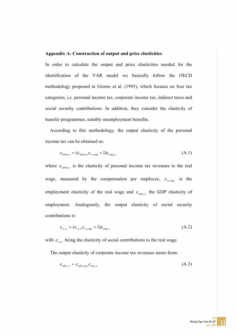
According to this methodology, the output elasticity of the personal

income tax can be obtained as:

yempempwwtdirhytdirh ,,,, )1( εεεε += (A.1)

where wtdirh,ε is the elasticity of personal income tax revenues to the real

wage, measured by the compensation per employee, empw,ε is the

employment elasticity of the real wage and yemp,ε the GDP elasticity of

employment. Analogously, the output elasticity of social security

contributions is:

yempempwwssyss ,,,, )1( εεεε += (A.2)

with wss,ε being the elasticity of social contributions to the real wage.

The output elasticity of corporate income tax revenues stems from:

ygosgostdircytdirc ,,, εεε = (A.3)

33ECB


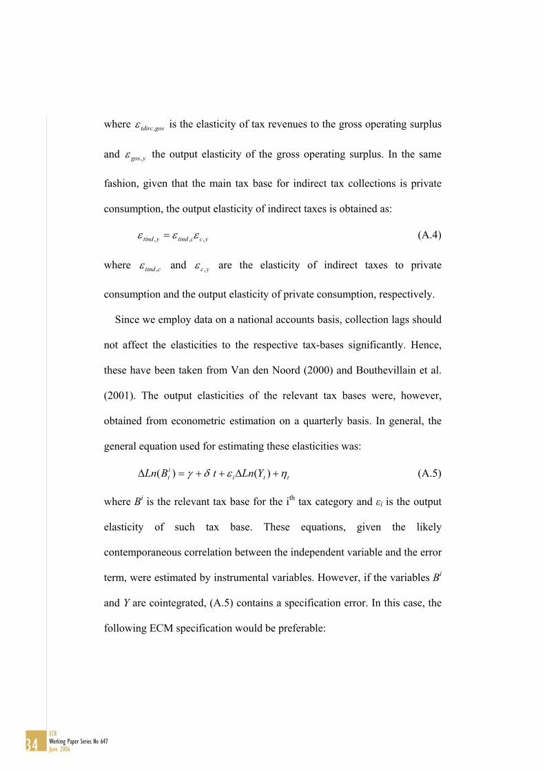
where gostdirc,ε is the elasticity of tax revenues to the gross operating surplus

and ygos,ε the output elasticity of the gross operating surplus. In the same

fashion, given that the main tax base for indirect tax collections is private

consumption, the output elasticity of indirect taxes is obtained as:

ycctindytind ,,, εεε = (A.4)

where ctind ,ε and yc,ε are the elasticity of indirect taxes to private

consumption and the output elasticity of private consumption, respectively.

Since we employ data on a national accounts basis, collection lags should

not affect the elasticities to the respective tax-bases significantly. Hence,

these have been taken from Van den Noord (2000) and Bouthevillain et al.

(2001). The output elasticities of the relevant tax bases were, however,

obtained from econometric estimation on a quarterly basis. In general, the

general equation used for estimating these elasticities was:

ttiit YLntBLn ηεδγ +∆++=∆ )( )( (A.5)

where Bi is the relevant tax base for the ith tax category and εi is the output

elasticity of such tax base. These equations, given the likely

contemporaneous correlation between the independent variable and the error

term, were estimated by instrumental variables. However, if the variables Bi

and Y are cointegrated, (A.5) contains a specification error. In this case, the

following ECM specification would be preferable:


t

k

j

ijtj

k

jjtj

titit

it

BLnYLn

YLntYLnBLnBLn

ηνϕ

εδφλµγ

+∆+∆+

∆+−−−+=∆

∑∑=

−=

−

−−

11

11

)()(

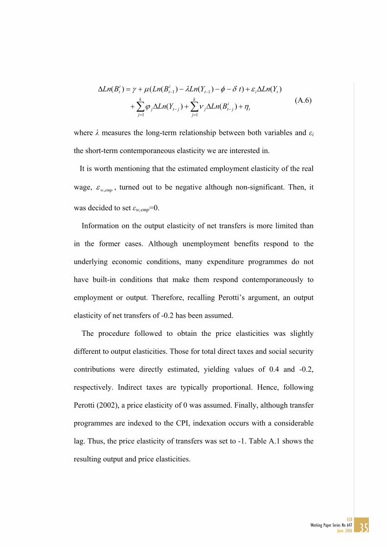
)() )()(()( (A.6)

where λ measures the long-term relationship between both variables and εi

the short-term contemporaneous elasticity we are interested in.

It is worth mentioning that the estimated employment elasticity of the real

wage, empw,ε , turned out to be negative although non-significant. Then, it

was decided to set εw,emp=0.

Information on the output elasticity of net transfers is more limited than

in the former cases. Although unemployment benefits respond to the

underlying economic conditions, many expenditure programmes do not

have built-in conditions that make them respond contemporaneously to

employment or output. Therefore, recalling Perotti’s argument, an output

elasticity of net transfers of -0.2 has been assumed.

The procedure followed to obtain the price elasticities was slightly

different to output elasticities. Those for total direct taxes and social security

contributions were directly estimated, yielding values of 0.4 and -0.2,

respectively. Indirect taxes are typically proportional. Hence, following

Perotti (2002), a price elasticity of 0 was assumed. Finally, although transfer

programmes are indexed to the CPI, indexation occurs with a considerable

lag. Thus, the price elasticity of transfers was set to -1. Table A.1 shows the

resulting output and price elasticities.

35ECB


References

Alesina, A., S. Ardagna, R. Perotti and F. Schiantarelli (2002) Fiscal Policy,

Profits and Investment, American Economic Review, 92, 571-589.

Blanchard, O.J. and R. Perotti (2002) An Empirical Characterization of the

Dynamic Effects of Changes in Government Spending and Taxes on

Output, Quarterly Journal of Economics, 117(4), 1329-1368.

Bouthevillain, C., P. Cour-Thimann, G. van den Dool, P. Hernández de Cos,

G. Langenus, M. Mohr, S. Momigliano and M. Tujula (2001)

Cyclically Adjusted Budget Balances: An Alternative Approach,

ECB Working Paper 77, September.

Burnside, C., M. Eichenbaum and J.D.M. Fisher (1999) Assessing the

Effects of Fiscal Shocks, mimeo, Northwestern University.

Canzoneri, M., R. Cumby, and B. Diba (2002) Should the European Central

Bank and the Federal Reserve be Concerned About Fiscal Policy,

paper prepared for the FRBKC’s Jackson Hole Symposium on

Rethinking Stabilization Policy, August.

De Castro, F., J.M. González-Páramo and P. Hernández de Cos (2004)

Fiscal Consolidation in Spain: Dynamic Interdependence of Public

Spending and Revenues, Investigaciones Económicas, vol.

XXXVIII(1), 193-207.


De Castro, F. (2005) The Macroeconomic Effects of Fiscal Policy in Spain,

Applied Economics, forthcoming.

Edelberg, W., M. Eichenbaum and J.D.M. Fisher (1998) Understanding the

Effects of a Shock to Government Purchases, NBER Working Paper

No 6737.

Estrada, A., J. L. Fernández, E. Moral and A. V. Regil (2004) A Quarterly

Macroeconometric Model of the Spanish Economy, Banco de

España, Working paper No 0413.

European Commission (2003) Public finances in EMU, European Economy,

Reports and Studies 3.

Fatás, A. and I. Mihov (2001) The Effects of Fiscal Policy on Consumption

and Employment: Theory and Evidence, CEPR Discussion Papers

2760, April.

Favero, C. (2002) How do European monetary and fiscal authorities

behave?, CEPR Discussion Paper Series, n.º 3426.

Galí, J., D. López-Salido and J. Vallés (2003) Understanding the Effects of

Government Spending on Consumption, Banco de España, Working

paper No 0321.

Galí, J. and R. Perotti (2003) Fiscal Policy and Monetary Integration in

Europe, NBER Working paper 9773.

37ECB


Giavazzi, F. and M. Pagano (1990) Can Severe Fiscal Contractions Be

Expansionary? Tales of Two Small European Countries, NBER

Macroeconomics Annual, 5, 75-111.

Giorno, C., P. Richardson, D. Roseveare and P. van den Noord (1995)

Potential Output, Output Gaps and Structural Budget Balances,

OECD Economic Studies 24.

Giudice, G., A. Turrini and J. in’t Veld (2003) Can Fiscal Consolidations Be

Expansionary in the EU? Ex-Post Evidence and Ex-ante Analysis,

European Commission, Economic Papers, 195, December.

Henry, J, P. Hernández de Cos and S. Momigliano (2004) The Short-Term

Impact of Government Budgets on Prices: Evidence from

Macroeconometric Models, Banco de España, Working paper No

0418.

Marcellino, M. (2002) Some Stylized Facts on Non-Systematic Fiscal

Policy in the Euro Area, CEPR Working Paper 3635, November.

Mountford, A. and H. Uhlig (2002) What are the effects of fiscal policy

shocks?, CEPR Working Paper 3338.

Neri, S. (2001) Assessing the effects of monetary and fiscal policy, Banca

d’Italia, Discussion Papers n.º 425, November.

Perotti, R. (1999) Fiscal Policy in Goods Times and Bad, Quarterly Journal

of Economics, 114(4), 1399-1436.


Perotti, R. (2001) What do we know about the effects of fiscal policy?, in

M. Bordignon and D. da Empoli (eds.), Politica Fiscale flessibilità

dei mercati e crescita, Franco Angeli, Milano.

Perotti, R. (2004) Estimating the Effects of Fiscal Policy in OECD

Countries, Proceedings, Federal Reserve Bank of San Francisco.

Ramey, V. and M. Shapiro (1998) Costly Capital Reallocation and the

Effects of Government Spending, NBER Working Paper 6283.

Van den Noord, P. (2000) The Size and Role of Automatic Fiscal Stabilizers

in the 1990s and Beyond, OECD Working Paper 230, January.

39ECB


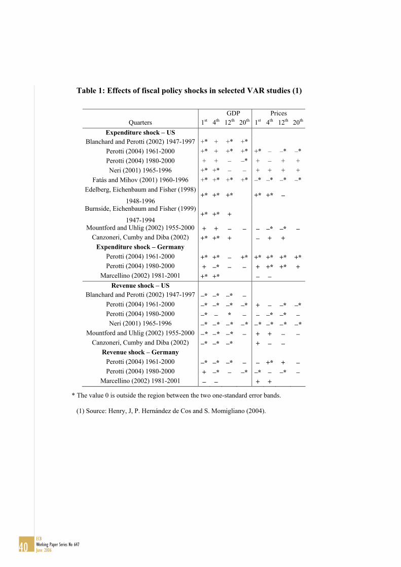
Table 1: Effects of fiscal policy shocks in selected VAR studies (1)

GDP Prices

Quarters 1st 4th 12th 20th 1st 4th 12th 20th Expenditure shock – US

Blanchard and Perotti (2002) 1947-1997 +* + +* +* Perotti (2004) 1961-2000 +* + +* +* +* – –* –* Perotti (2004) 1980-2000 + + – –* + – + + Neri (2001) 1965-1996 +* +* – – + + + +

Fatás and Mihov (2001) 1960-1996 +* +* +* +* –* –* –* –* Edelberg, Eichenbaum and Fisher (1998)

1948-1996 +* +* +* +* +* –

Burnside, Eichenbaum and Fisher (1999)

1947-1994 +* +* +

Mountford and Uhlig (2002) 1955-2000 + + – – – –* –* – Canzoneri, Cumby and Diba (2002) +* +* + – + +

Expenditure shock – Germany Perotti (2004) 1961-2000 +* +* – +* +* +* +* +* Perotti (2004) 1980-2000 + –* – – + +* +* +

Marcellino (2002) 1981-2001 +* +* – – Revenue shock – US

Blanchard and Perotti (2002) 1947-1997 –* –* –* – Perotti (2004) 1961-2000 –* –* –* –* + – –* –* Perotti (2004) 1980-2000 –* – * – – –* –* – Neri (2001) 1965-1996 –* –* –* –* –* –* –* –*

Mountford and Uhlig (2002) 1955-2000 –* –* –* – + + – – Canzoneri, Cumby and Diba (2002) –* –* –* + – –

Revenue shock – Germany Perotti (2004) 1961-2000 –* –* –* – – +* + – Perotti (2004) 1980-2000 + –* – –* –* – –* –

Marcellino (2002) 1981-2001 – – + +

* The value 0 is outside the region between the two one-standard error bands.

(1) Source: Henry, J, P. Hernández de Cos and S. Momigliano (2004).


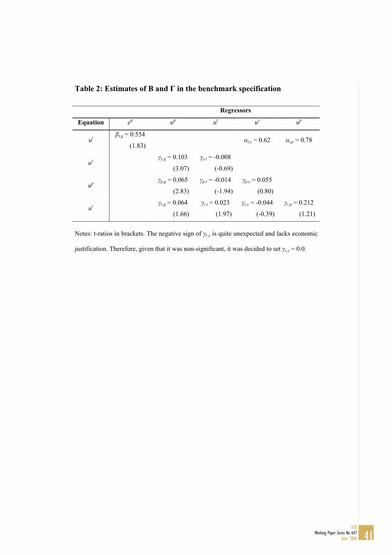
Table 2: Estimates of Β and Γ in the benchmark specification

Regressors

Equation eg ug ut uy up

ut βt,g = 0.554

(1.83) αt,y = 0.62 αt,p = 0.78

uy γy,g = 0.103

(3.07)

γy,t = -0.008

(-0.69)

up γp,g = 0.065

(2.83)

γp,t = -0.014

(-1.94)

γp,y = 0.055

(0.80)

ur γr,g = 0.064

(1.66)

γr,t = 0.023

(1.97)

γr,y = -0.044

(-0.39)

γr,p = 0.212

(1.21)

Notes: t-ratios in brackets. The negative sign of γr,y is quite unexpected and lacks economic

justification. Therefore, given that it was non-significant, it was decided to set γr,y = 0.0.

41ECB


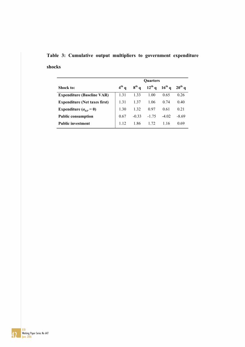
Table 3: Cumulative output multipliers to government expenditure

shocks

Quarters

Shock to: 4th q 8th q 12th q 16th q 20th q

Expenditure (Baseline VAR) 1.31 1.33 1.00 0.65 0.26

Expenditure (Net taxes first) 1.31 1.37 1.06 0.74 0.40

Expenditure (αg,p = 0) 1.30 1.32 0.97 0.61 0.21

Public consumption 0.67 -0.33 -1.75 -4.02 -8.69

Public investment 1.12 1.86 1.72 1.16 0.69


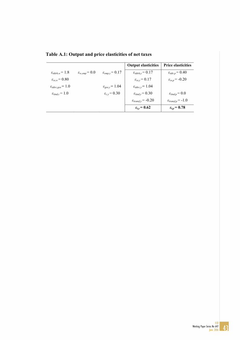
Table A.1: Output and price elasticities of net taxes

Output elasticities Price elasticities εtdirh,w = 1.8 εw,emp = 0.0 εemp,y = 0.17 εtdirh,y = 0.17 εtdir,p = 0.40

εss,w = 0.80 εss,y = 0.17 εss,p = -0.20

εtdirc,gos = 1.0 εgos,y = 1.04 εtdirc,y = 1.04

εtind,c = 1.0 εc,y = 0.30 εtind,y = 0.30 εtind,p = 0.0

εtransf,y = -0.20 εtransf,p = -1.0 εt,y = 0.62 εt,p = 0.78

43ECB


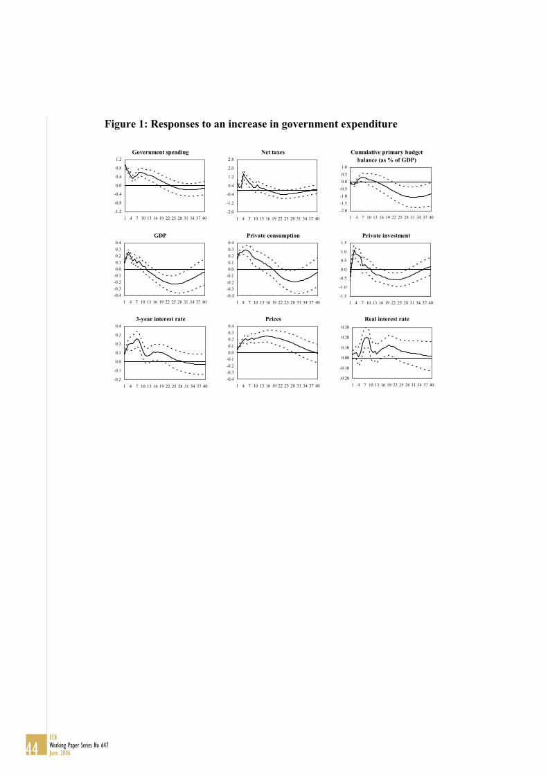
Figure 1: Responses to an increase in government expenditure

Government spending

-1.2

-0.8

-0.4

0.0

0.4

0.8

1.2

1 4 7 10 13 16 19 22 25 28 31 34 37 40

Cumulative primary budget balance (as % of GDP)

-2.0-1.5-1.0-0.50.00.51.0

1 4 7 10 13 16 19 22 25 28 31 34 37 40

Real interest rate

-0.20

-0.10

0.00

0.10

0.20

0.30

1 4 7 10 13 16 19 22 25 28 31 34 37 40

Net taxes

-2.0

-1.2

-0.4

0.4

1.2

2.0

2.8

1 4 7 10 13 16 19 22 25 28 31 34 37 40

GDP

-0.4-0.3-0.2-0.10.00.10.20.30.4

1 4 7 10 13 16 19 22 25 28 31 34 37 40

Prices

-0.4-0.3-0.2-0.10.00.10.20.30.4

1 4 7 10 13 16 19 22 25 28 31 34 37 40

3-year interest rate

-0.2

-0.1

0.0

0.1

0.2

0.3

0.4

1 4 7 10 13 16 19 22 25 28 31 34 37 40

Private consumption

-0.4-0.3-0.2-0.10.00.10.20.30.4

1 4 7 10 13 16 19 22 25 28 31 34 37 40

Private investment

-1.5

-1.0

-0.5

0.0

0.5

1.0

1.5

1 4 7 10 13 16 19 22 25 28 31 34 37 40


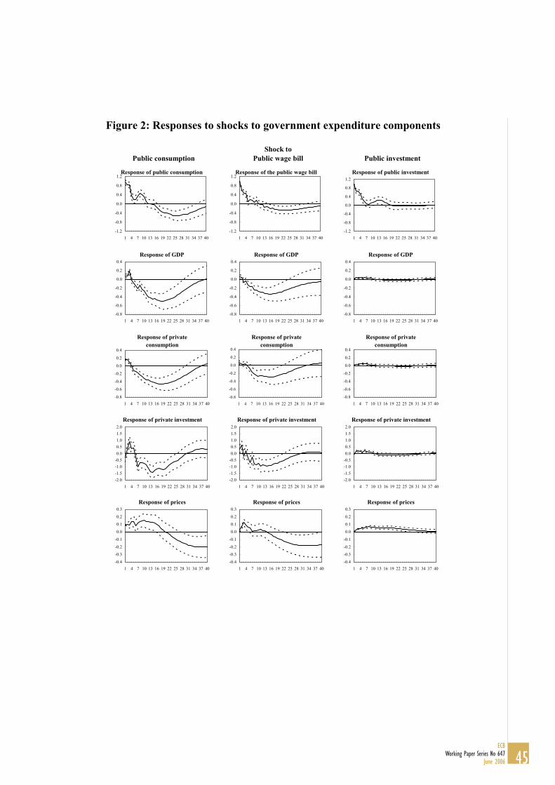
Figure 2: Responses to shocks to government expenditure components

Public investmentPublic consumptionShock to

Public wage bill

Response of public consumption

-1.2

-0.8

-0.4

0.0

0.4

0.8

1.2

1 4 7 10 13 16 19 22 25 28 31 34 37 40

Response of GDP

-0.8

-0.6

-0.4

-0.2

0.0

0.2

0.4

1 4 7 10 13 16 19 22 25 28 31 34 37 40

Response of private consumption

-0.8

-0.6

-0.4

-0.2

0.0

0.2

0.4

1 4 7 10 13 16 19 22 25 28 31 34 37 40

Response of private investment

-2.0-1.5-1.0-0.50.00.51.01.52.0

1 4 7 10 13 16 19 22 25 28 31 34 37 40

Response of public investment

-1.2

-0.8

-0.4

0.0

0.4

0.8

1.2

1 4 7 10 13 16 19 22 25 28 31 34 37 40


-0.8

-0.6

-0.4

-0.2

0.0

0.2

0.4

1 4 7 10 13 16 19 22 25 28 31 34 37 40

Response of GDP

-0.8

-0.6

-0.4

-0.2

0.0

0.2

0.4

1 4 7 10 13 16 19 22 25 28 31 34 37 40


-2.0-1.5-1.0-0.50.00.51.01.52.0

1 4 7 10 13 16 19 22 25 28 31 34 37 40

Response of the public wage bill

-1.2

-0.8

-0.4

0.0

0.4

0.8

1.2

1 4 7 10 13 16 19 22 25 28 31 34 37 40

Response of GDP

-0.8

-0.6

-0.4

-0.2

0.0

0.2

0.4

1 4 7 10 13 16 19 22 25 28 31 34 37 40


-0.8

-0.6

-0.4

-0.2

0.0

0.2

0.4

1 4 7 10 13 16 19 22 25 28 31 34 37 40


-2.0-1.5-1.0-0.50.00.51.01.52.0

1 4 7 10 13 16 19 22 25 28 31 34 37 40

Response of prices

-0.4

-0.3

-0.2

-0.1

0.0

0.1

0.2

0.3

1 4 7 10 13 16 19 22 25 28 31 34 37 40

Response of prices

-0.4

-0.3

-0.2

-0.1

0.0

0.1

0.2

0.3

1 4 7 10 13 16 19 22 25 28 31 34 37 40

Response of prices

-0.4

-0.3

-0.2

-0.1

0.0

0.1

0.2

0.3

1 4 7 10 13 16 19 22 25 28 31 34 37 40

45ECB


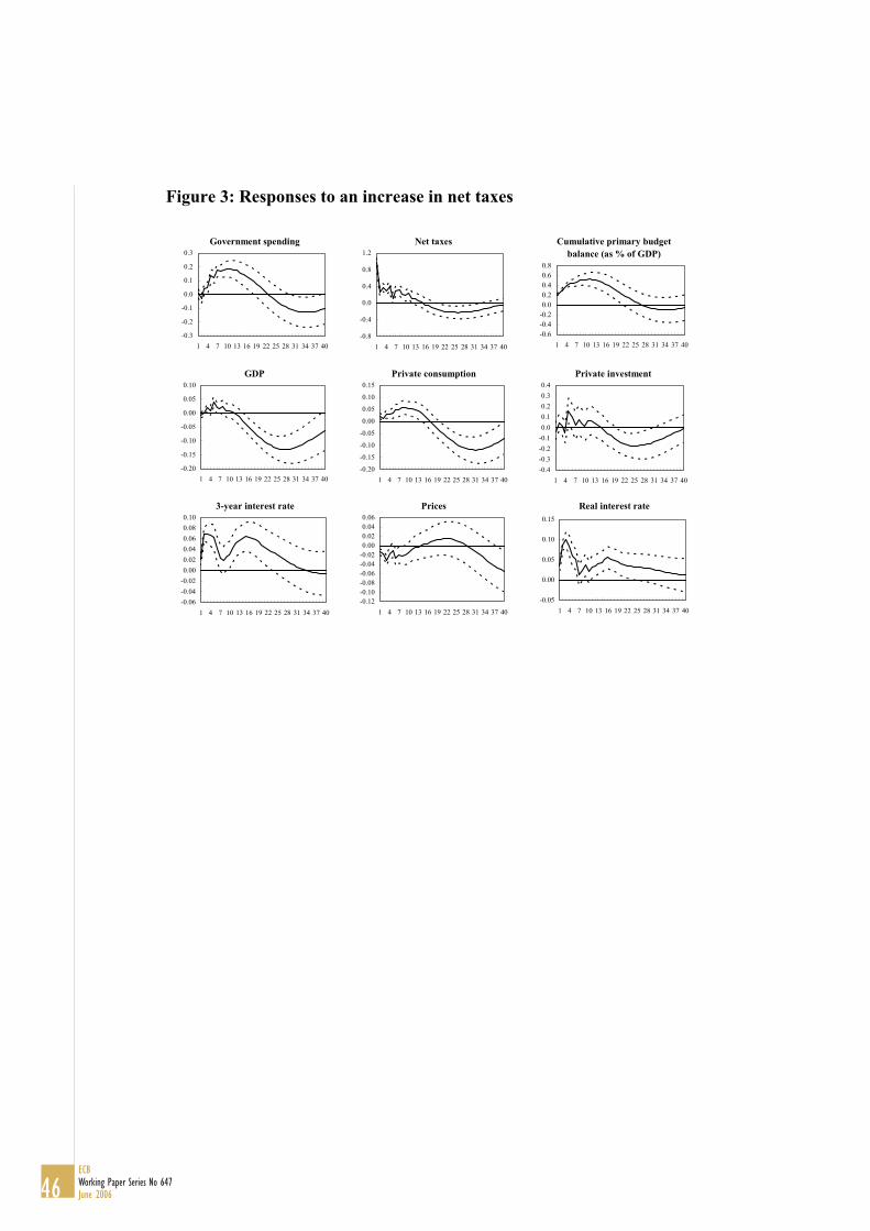
Figure 3: Responses to an increase in net taxes

Government spending

-0.3

-0.2

-0.1

0.0

0.1

0.2

0.3

1 4 7 10 13 16 19 22 25 28 31 34 37 40

Cumulative primary budget balance (as % of GDP)

-0.6-0.4-0.20.00.20.40.60.8

1 4 7 10 13 16 19 22 25 28 31 34 37 40

Real interest rate

-0.05

0.00

0.05

0.10

0.15

1 4 7 10 13 16 19 22 25 28 31 34 37 40

Net taxes

-0.8

-0.4

0.0

0.4

0.8

1.2

1 4 7 10 13 16 19 22 25 28 31 34 37 40

GDP

-0.20

-0.15

-0.10

-0.05

0.00

0.05

0.10

1 4 7 10 13 16 19 22 25 28 31 34 37 40

Prices

-0.12-0.10-0.08-0.06-0.04-0.020.000.020.040.06

1 4 7 10 13 16 19 22 25 28 31 34 37 40

3-year interest rate

-0.06-0.04-0.020.000.020.040.060.080.10

1 4 7 10 13 16 19 22 25 28 31 34 37 40

Private consumption

-0.20

-0.15

-0.10

-0.05

0.00

0.05

0.10

0.15

1 4 7 10 13 16 19 22 25 28 31 34 37 40

Private investment

-0.4-0.3-0.2-0.10.00.10.20.30.4

1 4 7 10 13 16 19 22 25 28 31 34 37 40


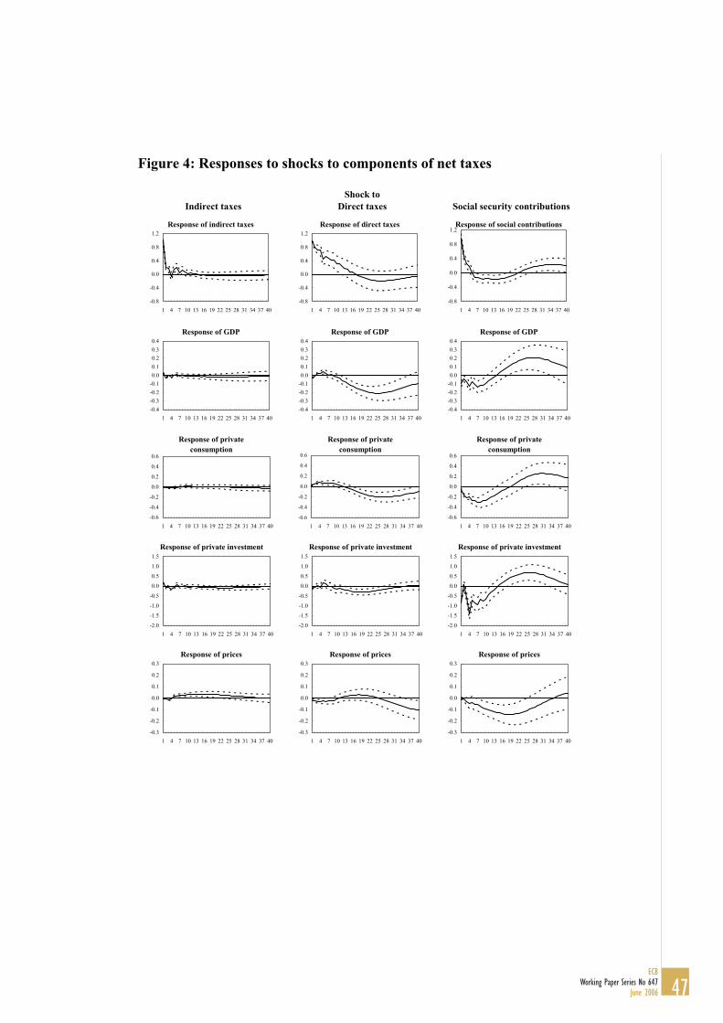
Figure 4: Responses to shocks to components of net taxes

Social security contributionsIndirect taxesShock to

Direct taxes

Response of indirect taxes

-0.8

-0.4

0.0

0.4

0.8

1.2

1 4 7 10 13 16 19 22 25 28 31 34 37 40

Response of GDP

-0.4-0.3-0.2-0.10.00.10.20.30.4

1 4 7 10 13 16 19 22 25 28 31 34 37 40


-0.6

-0.4

-0.2

0.0

0.2

0.4

0.6

1 4 7 10 13 16 19 22 25 28 31 34 37 40


-2.0

-1.5

-1.0

-0.5

0.0

0.5

1.0

1.5

1 4 7 10 13 16 19 22 25 28 31 34 37 40

Response of social contributions

-0.8

-0.4

0.0

0.4

0.8

1.2

1 4 7 10 13 16 19 22 25 28 31 34 37 40


-0.6

-0.4

-0.2

0.0

0.2

0.4

0.6

1 4 7 10 13 16 19 22 25 28 31 34 37 40

Response of GDP

-0.4-0.3-0.2-0.10.00.10.20.30.4

1 4 7 10 13 16 19 22 25 28 31 34 37 40


-2.0

-1.5

-1.0

-0.5

0.0

0.5

1.0

1.5

1 4 7 10 13 16 19 22 25 28 31 34 37 40

Response of direct taxes

-0.8

-0.4

0.0

0.4

0.8

1.2

1 4 7 10 13 16 19 22 25 28 31 34 37 40

Response of GDP

-0.4-0.3-0.2-0.10.00.10.20.30.4

1 4 7 10 13 16 19 22 25 28 31 34 37 40


-0.6

-0.4

-0.2

0.0

0.2

0.4

0.6

1 4 7 10 13 16 19 22 25 28 31 34 37 40


-2.0

-1.5

-1.0

-0.5

0.0

0.5

1.0

1.5

1 4 7 10 13 16 19 22 25 28 31 34 37 40

Response of prices

-0.3

-0.2

-0.1

0.0

0.1

0.2

0.3

1 4 7 10 13 16 19 22 25 28 31 34 37 40

Response of prices

-0.3

-0.2

-0.1

0.0

0.1

0.2

0.3

1 4 7 10 13 16 19 22 25 28 31 34 37 40

Response of prices

-0.3

-0.2

-0.1

0.0

0.1

0.2

0.3

1 4 7 10 13 16 19 22 25 28 31 34 37 40

47ECB


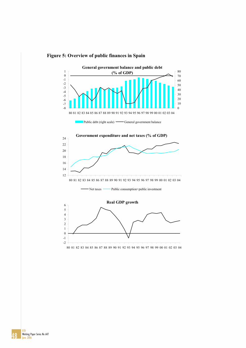
Figure 5: Overview of public finances in Spain

General government balance and public debt (% of GDP)

-8-7-6-5-4-3-2-101

80 81 82 83 84 85 86 87 88 89 90 91 92 93 94 95 96 97 98 99 00 01 02 03 0401020304050607080

Public debt (right scale) General government balance

Government expenditure and net taxes (% of GDP)

12

14

16

18

20

22

24

80 81 82 83 84 85 86 87 88 89 90 91 92 93 94 95 96 97 98 99 00 01 02 03 04

Net taxes Public consumption+public investment

Real GDP growth

-2-10123456

80 81 82 83 84 85 86 87 88 89 90 91 92 93 94 95 96 97 98 99 00 01 02 03 04


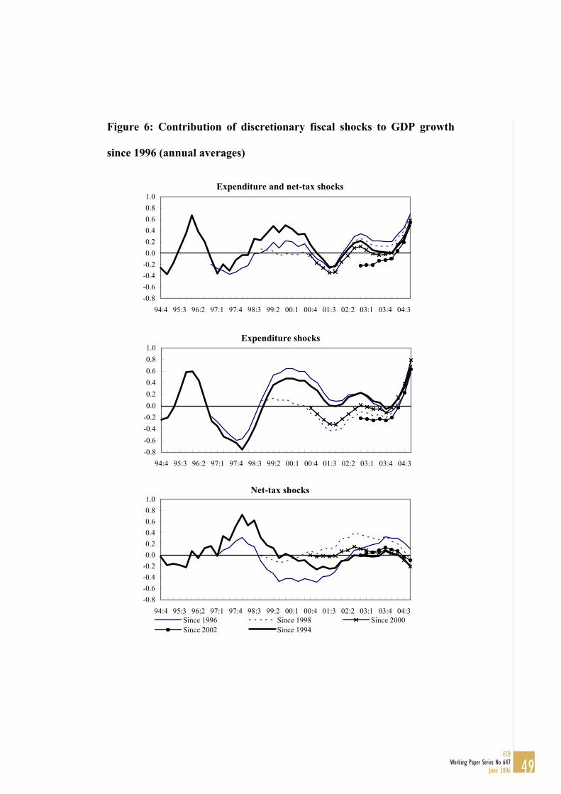
Figure 6: Contribution of discretionary fiscal shocks to GDP growth

since 1996 (annual averages)

Expenditure and net-tax shocks

-0.8-0.6-0.4-0.20.00.20.40.60.81.0

94:4 95:3 96:2 97:1 97:4 98:3 99:2 00:1 00:4 01:3 02:2 03:1 03:4 04:3

Expenditure shocks

-0.8-0.6-0.4-0.20.00.20.40.60.81.0

94:4 95:3 96:2 97:1 97:4 98:3 99:2 00:1 00:4 01:3 02:2 03:1 03:4 04:3

Net-tax shocks

-0.8-0.6-0.4-0.20.00.20.40.60.81.0

94:4 95:3 96:2 97:1 97:4 98:3 99:2 00:1 00:4 01:3 02:2 03:1 03:4 04:3Since 1996 Since 1998 Since 2000Since 2002 Since 1994

49ECB


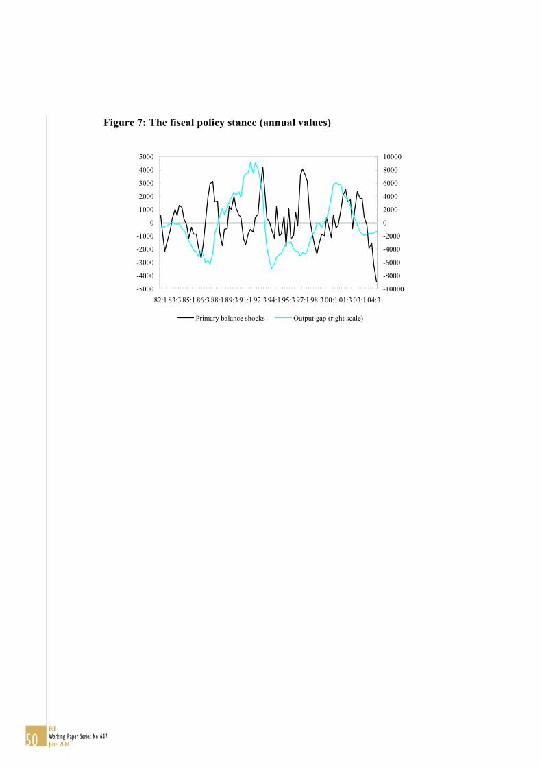
Figure 7: The fiscal policy stance (annual values)

-5000

-4000

-3000

-2000

-1000

0

1000

2000

3000

4000

5000

82:1 83:3 85:1 86:3 88:1 89:3 91:1 92:3 94:1 95:3 97:1 98:3 00:1 01:3 03:1 04:3-10000

-8000

-6000

-4000

-2000

0

2000

4000

6000

8000

10000

Primary balance shocks Output gap (right scale)


51ECB


European Central Bank Working Paper Series

For a complete list of Working Papers published by the ECB, please visit the ECB’s website(http://www.ecb.int)

594 “The euro’s trade effects” by R. Baldwin, comments by J. A. Frankel and J. Melitz, March 2006

595 “Trends and cycles in the euro area: how much heterogeneity and should we worry about it?”by D. Giannone and L. Reichlin, comments by B. E. Sørensen and M. McCarthy, March 2006.

596 “The effects of EMU on structural reforms in labour and product markets” by R. Duvaland J. Elmeskov, comments by S. Nickell and J. F. Jimeno, March 2006.

597 “Price setting and inflation persistence: did EMU matter?” by I. Angeloni, L. Aucremanne,M. Ciccarelli, comments by W. T. Dickens and T. Yates, March 2006.

598 “The impact of the euro on financial markets” by L. Cappiello, P. Hördahl, A. Kadarejaand S. Manganelli, comments by X. Vives and B. Gerard, March 2006.

599 “What effects is EMU having on the euro area and its Member Countries? An overview”by F. P. Mongelli and J. L. Vega, March 2006.

600 “A speed limit monetary policy rule for the euro area” by L. Stracca, April 2006.

601 “Excess burden and the cost of inefficiency in public services provision” by A. Afonsoand V. Gaspar, April 2006.

602 “Job flow dynamics and firing restrictions: evidence from Europe” by J. Messina and G. Vallanti,April 2006.

603 “Estimating multi-country VAR models” by F. Canova and M. Ciccarelli, April 2006.

604 “A dynamic model of settlement” by T. Koeppl, C. Monnet and T. Temzelides, April 2006.

605 “(Un)Predictability and macroeconomic stability” by A. D’Agostino, D. Giannone and P. Surico,April 2006.

606 “Measuring the importance of the uniform nonsynchronization hypothesis” by D. A. Dias,C. Robalo Marques and J. M. C. Santos Silva, April 2006.

607 “Price setting behaviour in the Netherlands: results of a survey” by M. Hoeberichts andA. Stokman, April 2006.

608 “How does information affect the comovement between interest rates and exchange rates?”by M. Sánchez, April 2006.

609 “The elusive welfare economics of price stability as a monetary policy objective: why NewKeynesian central bankers should validate core inflation” by W. H. Buiter, April 2006.

610 “Real-time model uncertainty in the United States: the Fed from 1996-2003” by R. J. Tetlowand B. Ironside, April 2006.


611 “Monetary policy, determinacy, and learnability in the open economy” by J. Bullardand E. Schaling, April 2006.

612 “Optimal fiscal and monetary policy in a medium-scale macroeconomic model”by S. Schmitt-Grohé and M. Uribe, April 2006.

613 “Welfare-based monetary policy rules in an estimated DSGE model of the US economy”by M. Juillard, P. Karam, D. Laxton and P. Pesenti, April 2006.

614 “Expenditure switching vs. real exchange rate stabilization: competing objectives forexchange rate policy” by M. B. Devereux and C. Engel, April 2006.

615 “Quantitative goals for monetary policy” by A. Fatás, I. Mihov and A. K. Rose, April 2006.

616 “Global financial transmission of monetary policy shocks” by M. Ehrmann and M. Fratzscher,April 2006.

617 “New survey evidence on the pricing behaviour of Luxembourg firms” by P. Lünnemannand T. Y. Mathä, May 2006.

618 “The patterns and determinants of price setting in the Belgian industry” by D. Cornilleand M. Dossche, May 2006.

619 “Cyclical inflation divergence and different labor market institutions in the EMU”by A. Campolmi and E. Faia, May 2006.

620 “Does fiscal policy matter for the trade account? A panel cointegration study” by K. Funkeand C. Nickel, May 2006.

621 “Assessing predetermined expectations in the standard sticky-price model: a Bayesian approach”by P. Welz, May 2006.

622 “Short-term forecasts of euro area real GDP growth: an assessment of real-time performancebased on vintage data” by M. Diron, May 2006.

623 “Human capital, the structure of production, and growth” by A. Ciccone andE. Papaioannou, May 2006.

624 “Foreign reserves management subject to a policy objective” by J. Coche, M. Koivu, K. Nyholmand V. Poikonen, May 2006.

625 “Sectoral explanations of employment in Europe: the role of services” by A. D’Agostino,R. Serafini and M. Ward-Warmedinger, May 2006.

626 “Financial integration, international portfolio choice and the European Monetary Union”by R. A. De Santis and B. Gérard, May 2006.

627 “Euro area banking sector integration: using hierarchical cluster analysis techniques”by C. Kok Sørensen, J. M. Puigvert Gutiérrez, May 2006.

53ECB


628 “Long-run money demand in the new EU Member States with exchange rate effects”by C. Dreger, H.-E. Reimers and B. Roffia, May 2006.

629 “A market microstructure analysis of foreign exchange intervention” by P. Vitale, May 2006.

630 “Implications of monetary union for catching-up member states” by M. Sánchez, May 2006.

631 “Which news moves the euro area bond market?” by M. Andersson, L. J. Hansen andS. Sebestyén, May 2006.

632 “Does information help recovering structural shocks from past observations?”by D. Giannone and L. Reichlin, May 2006.

633 “Nowcasting GDP and inflation: the real-time informational content of macroeconomic datareleases” by D. Giannone, L. Reichlin and D. H. Small, May 2006.

634 “Expenditure reform in industrialised countries: a case study approach” by S. Hauptmeier,M. Heipertz and L. Schuknecht, May 2006.

635 “Identifying the role of labor markets for monetary policy in an estimated DSGE model”by K. Christoffel, K. Kuester and T. Linzert, June 2006.

636 “Exchange rate stabilization in developed and underdeveloped capital markets”by V. Chmelarova and G. Schnabl, June 2006.

637 “Transparency, expectations, and forecasts” by A. Bauer, R. Eisenbeis, D. Waggoner andT. Zha, June 2006.

638 “Detecting and predicting forecast breakdowns” by R. Giacomini and B. Rossi, June 2006.

639 “Optimal monetary policy with uncertainty about financial frictions” by R. Moessner, June 2006.

640 “Employment stickiness in small manufacturing firms” by P. Vermeulen, June 2006.

641 “A factor risk model with reference returns for the US dollar and Japanese yen bond markets”by C. Bernadell, J. Coche and K. Nyholm, June 2006.

642 “Financing constraints and firms’ cash policy in the euro area” by R. Pál and A. Ferrando, June 2006.

643 “Inflation forecast-based-rules and indeterminacy: a puzzle and a resolution” by P. Levine,P. McAdam and J. Pearlman, June 2006.

644 “Adaptive learning, persistence, and optimal monetary policy” by V. Gaspar, F. Smets andD. Vestin, June 2006.

645 “Are internet prices sticky?” by P. Lünnemann and L. Wintr, June 2006.

646 “The Dutch block of the ESCB multi-country model” by E. Angelini, F. Boissay andM. Ciccarelli, June 2006.

647 “The economic effects of exogenous fiscal shocks in Spain: a SVAR approach”by F. de Castro Fernández and P. Hernández de Cos, June 2006.

ISSN 1561081-0

9 7 7 1 5 6 1 0 8 1 0 0 5

Documents

The economic effects of exogenous fiscal shocks in Spain ... · issn 1561081-0 9 771561 081005 working paper series no 647 / june 2006 the economic effects of exogenous fiscal shocks