Embed Size (px)
Citation preview

Agriculture 5-33
The IPCC (2006) Tier 1 methodology was used to estimate direct N2O emissions for mineral cropland soils that are
not simulated by DAYCENT. For the Tier 1 Approach, estimates of direct N2O emissions from N applications were
based on mineral soil N that was made available from the following practices: (1) the application of synthetic
commercial fertilizers; (2) application of managed manure and non-manure commercial organic fertilizers; and (3)
the retention of above- and below-ground crop residues in agricultural fields (i.e., crop biomass that is not
harvested). Non-manure, commercial organic amendments were not included in the DAYCENT simulations
because county-level data were not available.14 Consequently, commercial organic fertilizer, as well as additional
manure that was not added to crops in the DAYCENT simulations, were included in the Tier 1 analysis. The
following sources were used to derive activity data:
A process-of-elimination approach was used to estimate synthetic N fertilizer additions for crop areas not
simulated by DAYCENT. The total amount of fertilizer used on farms has been estimated at the county-
level by the USGS from sales records (Ruddy et al. 2006), and these data were aggregated to obtain state-
level N additions to farms. For 2002 through 2013, state-level fertilizer for on-farm use is adjusted based on
annual fluctuations in total U.S. fertilizer sales (AAPFCO 1995 through 2007, AAPFCO 2008 through
2014).15 After subtracting the portion of fertilizer applied to crops and grasslands simulated by DAYCENT
(see Tier 3 Approach for Cropland Mineral Soils Section and Grasslands Section for information on data
sources), the remainder of the total fertilizer used on farms was assumed to be applied to crops that were
not simulated by DAYCENT.
Similarly, a process-of-elimination approach was used to estimate manure N additions for crops that were
not simulated by DAYCENT. The amount of manure N applied in the Tier 3 approach to crops and
grasslands was subtracted from total manure N available for land application (see Tier 3 Approach for
Cropland Mineral Soils Section and Grasslands Section for information on data sources), and this
difference was assumed to be applied to crops that are not simulated by DAYCENT.
Commercial organic fertilizer additions were based on organic fertilizer consumption statistics, which were
converted to units of N using average organic fertilizer N content (TVA 1991 through 1994; AAPFCO
1995 through 2011). Commercial fertilizers do include some manure and sewage sludge, but the amounts
are removed from the commercial fertilizer data to avoid double counting with the manure N dataset
described above and the sewage sludge amendment data discussed later in this section.
Crop residue N was derived by combining amounts of above- and below-ground biomass, which were
determined based on crop production yield statistics (USDA-NASS 2014), dry matter fractions (IPCC
2006), linear equations to estimate above-ground biomass given dry matter crop yields from harvest (IPCC
2006), ratios of below-to-above-ground biomass (IPCC 2006), and N contents of the residues (IPCC 2006).
The total increase in soil mineral N from applied fertilizers and crop residues was multiplied by the IPCC (2006)
default emission factor to derive an estimate of direct N2O emissions using the Tier 1 Approach.
Drainage of Organic Soils in Croplands and Grasslands
The IPCC (2006) Tier 1 methods were used to estimate direct N2O emissions due to drainage of organic soils in
croplands or grasslands at a state scale. State-scale estimates of the total area of drained organic soils were obtained
from the 2009 NRI (USDA-NRCS 2009) using soils data from the Soil Survey Geographic Database (SSURGO)
(Soil Survey Staff 2011). Temperature data from Daly et al. (1994, 1998) were used to subdivide areas into
temperate and tropical climates using the climate classification from IPCC (2006). Annual data were available
between 1990 and 2007. Emissions are assumed to be similar to 2007 from 2008 to 2013 because no additional
activity data are currently available from the NRI for the latter years. To estimate annual emissions, the total
temperate area was multiplied by the IPCC default emission factor for temperate regions, and the total tropical area
was multiplied by the IPCC default emission factor for tropical regions (IPCC 2006).
14 Commercial organic fertilizers include dried blood, tankage, compost, and other, but the dried manure and sewage sludge is
removed from the dataset in order to avoid double counting with other datasets that are used for manure N and sewage sludge.
15 Values were not available for 2013 so a “least squares line” statistical extrapolation using the previous 5 years of data is used
to arrive at an approximate value.

5-34 Inventory of U.S. Greenhouse Gas Emissions and Sinks: 1990–2013
Direct N2O Emissions from Grassland Soils
As with N2O from croplands, the Tier 3 process-based DAYCENT model and Tier 1 method described in IPCC
(2006) were combined to estimate emissions from non-federal grasslands and PRP manure N additions for federal
grasslands, respectively. Grassland includes pasture and rangeland that produce grass forage primarily for livestock
grazing. Rangelands are typically extensive areas of native grassland that are not intensively managed, while
pastures are typically seeded grassland (possibly following tree removal) that may also have addition management,
such as irrigation or interseeding legumes. DAYCENT was used to simulate N2O emissions from NRI survey
locations (USDA-NRCS 2009) on non-federal grasslands resulting from manure deposited by livestock directly onto
pastures and rangelands (i.e., PRP manure), N fixation from legume seeding, managed manure amendments (i.e.,
manure other than PRP manure such as Daily Spread), and synthetic fertilizer application. Other N inputs were
simulated within the DAYCENT framework, including N input from mineralization due to decomposition of soil
organic matter and N inputs from senesced grass litter, as well as asymbiotic fixation of N from the atmosphere. The
simulations used the same weather, soil, and synthetic N fertilizer data as discussed under the Tier 3 Approach for
Mineral Cropland Soils section. Managed manure N amendments to grasslands were estimated from Edmonds et al.
(2003) and adjusted for annual variation using data on the availability of managed manure N for application to soils,
according to methods described in the Manure Management section (5.2 Manure Management (IPCC Source
Category 3B)) and Annex 3.11. Biological N fixation is simulated within DAYCENT, and therefore was not an
input to the model.
Manure N deposition from grazing animals in PRP systems (i.e., PRP manure) is another key input of N to
grasslands. The amounts of PRP manure N applied on non-federal grasslands for each NRI point were based on
amount of N excreted by livestock in PRP systems. The total amount of N excreted in each county was divided by
the grassland area to estimate the N input rate associated with PRP manure. The resulting input rates were used in
the DAYCENT simulations. DAYCENT simulations of non-federal grasslands accounted for approximately 68
percent of total PRP manure N in aggregate across the country. The remainder of the PRP manure N in each state
was assumed to be excreted on federal grasslands, and the N2O emissions were estimated using the IPCC (2006)
Tier 1 method with IPCC default emission factors. Sewage sludge was assumed to be applied on grasslands because
of the heavy metal content and other pollutants in human waste that limit its use as an amendment to croplands.
Sewage sludge application was estimated from data compiled by EPA (1993, 1999, 2003), McFarland (2001), and
NEBRA (2007). Sewage sludge data on soil amendments to agricultural lands were only available at the national
scale, and it was not possible to associate application with specific soil conditions and weather at the county scale.
Therefore, DAYCENT could not be used to simulate the influence of sewage sludge amendments on N2O emissions
from grassland soils, and consequently, emissions from sewage sludge were estimated using the IPCC (2006) Tier 1
method.
Grassland area data were consistent with the Land Representation reported in Section 0 for the conterminous United
States. Data were obtained from the U.S. Department of Agriculture NRI (Nusser and Goebel 1998) and the U.S.
Geological Survey (USGS) National Land Cover Dataset (Vogelman et al. 2001), which were reconciled with the
Forest Inventory and Analysis Data. The area data for pastures and rangeland were aggregated to the county level to
estimate non-federal and federal grassland areas.
N2O emissions for the PRP manure N deposited on federal grasslands and applied sewage sludge N were estimated
using the Tier 1 method by multiplying the N input by the appropriate emission factor. Emissions from manure N
were estimated at the state level and aggregated to the entire country, but emissions from sewage sludge N were
calculated exclusively at the national scale.
As previously mentioned, each NRI point was simulated 100 times as part of the uncertainty assessment, yielding a
total of over 18 million simulation runs for the analysis. Soil N2O emission estimates from DAYCENT were
adjusted using a structural uncertainty estimator accounting for uncertainty in model algorithms and parameter
values (Del Grosso et al. 2010). Soil N2O emissions and 95 percent confidence intervals were estimated for each
year between 1990 and 2007, but emissions from 2008 to 2013 were assumed to be similar to 2007. The annual data
are currently available through 2010 (USDA-NRCS 2013). However, this Inventory only uses NRI data through
2007 because newer data were not made available in time to incorporate the additional years into this Inventory.

Agriculture 5-35
Total Direct N2O Emissions from Cropland and Grassland Soils
Annual direct emissions from the Tier 1 and 3 approaches for cropland mineral soils, from drainage and cultivation
of organic cropland soils, and from grassland soils were summed to obtain the total direct N2O emissions from
agricultural soil management (see Table 5-18 and Table 5-19).
Indirect N2O Emissions
This section describes the methods used for estimating indirect soil N2O emissions from croplands and grasslands.
Indirect N2O emissions occur when mineral N made available through anthropogenic activity is transported from the
soil either in gaseous or aqueous forms and later converted into N2O. There are two pathways leading to indirect
emissions. The first pathway results from volatilization of N as NOx and NH3 following application of synthetic
fertilizer, organic amendments (e.g., manure, sewage sludge), and deposition of PRP manure. N made available
from mineralization of soil organic matter and residue, including N incorporated into crops and forage from
symbiotic N fixation, and input of N from asymbiotic fixation also contributes to volatilized N emissions.
Volatilized N can be returned to soils through atmospheric deposition, and a portion of the deposited N is emitted to
the atmosphere as N2O. The second pathway occurs via leaching and runoff of soil N (primarily in the form of NO3)
that was made available through anthropogenic activity on managed lands, mineralization of soil organic matter and
residue, including N incorporated into crops and forage from symbiotic N fixation, and inputs of N into the soil from
asymbiotic fixation. The NO3- is subject to denitrification in water bodies, which leads to N2O emissions.
Regardless of the eventual location of the indirect N2O emissions, the emissions are assigned to the original source
of the N for reporting purposes, which here includes croplands and grasslands.
Indirect N2O Emissions from Atmospheric Deposition of Volatilized N
The Tier 3 DAYCENT model and IPCC (2006) Tier 1 methods were combined to estimate the amount of N that was
volatilized and eventually emitted as N2O. DAYCENT was used to estimate N volatilization for land areas whose
direct emissions were simulated with DAYCENT (i.e., most commodity and some specialty crops and most
grasslands). The N inputs included are the same as described for direct N2O emissions in the Tier 3 Approach for
Cropland Mineral Soils Section and Grasslands Section. N volatilization for all other areas was estimated using the
Tier 1 method and default IPCC fractions for N subject to volatilization (i.e., N inputs on croplands not simulated by
DAYCENT, PRP manure N excreted on federal grasslands, sewage sludge application on grasslands). For the
volatilization data generated from both the DAYCENT and Tier 1 approaches, the IPCC (2006) default emission
factor was used to estimate indirect N2O emissions occurring due to re-deposition of the volatilized N (Table 5-21).
Indirect N2O Emissions from Leaching/Runoff
As with the calculations of indirect emissions from volatilized N, the Tier 3 DAYCENT model and IPCC (2006)
Tier 1 method were combined to estimate the amount of N that was subject to leaching and surface runoff into water
bodies, and eventually emitted as N2O. DAYCENT was used to simulate the amount of N transported from lands in
the Tier 3 Approach. N transport from all other areas was estimated using the Tier 1 method and the IPCC (2006)
default factor for the proportion of N subject to leaching and runoff. This N transport estimate includes N
applications on croplands that were not simulated by DAYCENT, sewage sludge amendments on grasslands, and
PRP manure N excreted on federal grasslands. For both the DAYCENT Tier 3 and IPCC (2006) Tier 1 methods,
nitrate leaching was assumed to be an insignificant source of indirect N2O in cropland and grassland systems in arid
regions as discussed in IPCC (2006). In the United States, the threshold for significant nitrate leaching is based on
the potential evapotranspiration (PET) and rainfall amount, similar to IPCC (2006), and is assumed to be negligible
in regions where the amount of precipitation plus irrigation does not exceed 80 percent of PET. For leaching and
runoff data estimated by the Tier 3 and Tier 1 approaches, the IPCC (2006) default emission factor was used to
estimate indirect N2O emissions that occur in groundwater and waterways (Table 5-21).
Uncertainty and Time-Series Consistency Uncertainty was estimated for each of the following five components of N2O emissions from agricultural soil
management: (1) direct emissions simulated by DAYCENT; (2) the components of indirect emissions (N volatilized

5-36 Inventory of U.S. Greenhouse Gas Emissions and Sinks: 1990–2013
and leached or runoff) simulated by DAYCENT; (3) direct emissions approximated with the IPCC (2006) Tier 1
method; (4) the components of indirect emissions (N volatilized and leached or runoff) approximated with the IPCC
(2006) Tier 1 method; and (5) indirect emissions estimated with the IPCC (2006) Tier 1 method. Uncertainty in
direct emissions, which account for the majority of N2O emissions from agricultural management, as well as the
components of indirect emissions calculated by DAYCENT were estimated with a Monte Carlo Analysis,
addressing uncertainties in model inputs and structure (i.e., algorithms and parameterization) (Del Grosso et al.
2010). Uncertainties in direct emissions calculated with the IPCC (2006) Approach 1 method, the proportion of
volatilization and leaching or runoff estimated with the IPCC (2006) Approach 1 method, and indirect N2O
emissions were estimated with a simple error propagation approach (IPCC 2006). Uncertainties from the Approach
1 and Approach 3 (i.e., DAYCENT) estimates were combined using simple error propagation (IPCC 2006).
Additional details on the uncertainty methods are provided in Annex 3.12. The combined uncertainty for direct soil
N2O emissions ranged from 16 percent below to 26 percent above the 2013 emissions estimate of 224.7 MMT CO2
Eq., and the combined uncertainty for indirect soil N2O emissions ranged from 46 percent below to 160 percent
above the 2013 estimate of 39.0 MMT CO2 Eq.
Table 5-22: Quantitative Uncertainty Estimates of N2O Emissions from Agricultural Soil Management in 2013 (MMT CO2 Eq. and Percent)
Source Gas
2013 Emission
Estimate Uncertainty Range Relative to Emission Estimate
(MMT CO2 Eq.) (MMT CO2 Eq.) (%)
Lower
Bound
Upper
Bound
Lower
Bound
Upper
Bound
Direct Soil N2O Emissions N2O 224.7 189.2 282.4 -16% 26%
Indirect Soil N2O Emissions N2O 39.0 21.2 101.6 -46% 160%
Note: Due to lack of data, uncertainties in managed manure N production, PRP manure N production, other organic
fertilizer amendments, and sewage sludge amendments to soils are currently treated as certain; these sources of
uncertainty will be included in future Inventories.
Additional uncertainty is associated with the lack of an estimation of N2O emissions for croplands and grasslands in
Hawaii and Alaska, with the exception of drainage for organic soils in Hawaii. Agriculture is not extensive in either
state, so the emissions are likely to be small compared to the conterminous United States.
Methodological recalculations were applied to the entire time series to ensure time-series consistency from 1990
through 2013. Details on the emission trends through time are described in more detail in the Methodology section
above.
QA/QC and Verification DAYCENT results for N2O emissions and NO3
- leaching were compared with field data representing various
cropland and grassland systems, soil types, and climate patterns (Del Grosso et al. 2005, Del Grosso et al. 2008), and
further evaluated by comparing to emission estimates produced using the IPCC (2006) Tier 1 method for the same
sites. N2O measurement data were available for 21 sites in the United States, 4 in Europe, and one in Australia,
representing over 60 different combinations of fertilizer treatments and cultivation practices. DAYCENT estimates
of N2O emissions were closer to measured values at most sites compared to the IPCC Tier 1 estimate (Figure 5-7).
In general, IPCC Tier 1 methodology tends to over-estimate emissions when observed values are low and under-
estimate emissions when observed values are high, while DAYCENT estimates are less biased. DAYCENT
accounts for key site-level factors (weather, soil characteristics, and management) that are not addressed in the IPCC
Tier 1 Method, and thus the model is better able to represent the variability in N2O emissions. Nitrate leaching data
were available for four sites in the United States, representing 12 different combinations of fertilizer
amendments/tillage practices. DAYCENT does have a tendency to under-estimate very high N2O emission rates;
estimates are increased to correct for this bias based on a statistical model derived from the comparison of model
estimates to measurements (See Annex 3.12 for more information). Regardless, the comparison demonstrates that
DAYCENT provides relatively high predictive capability for N2O emissions and NO3- leaching, and is an
improvement over the IPCC Tier 1 method.

Agriculture 5-37
Figure 5-7: Comparison of Measured Emissions at Field Sites and Modeled Emissions Using
the DAYCENT Simulation Model and IPCC Tier 1 Approach.
Spreadsheets containing input data and probability distribution functions required for DAYCENT simulations of
croplands and grasslands and unit conversion factors were checked, as were the program scripts that were used to
run the Monte Carlo uncertainty analysis. Links between spreadsheets were checked, updated, and corrected when
necessary. Spreadsheets containing input data, emission factors, and calculations required for the Tier 1 approach
were checked and an error was found relating to residue N inputs. Some crops that were simulated by DAYCENT
were also included in the Tier 1 method. To correct this double-counting of N inputs, residue inputs from crops
simulated by DAYCENT were removed from the Tier 1 calculations.
Recalculations Discussion For the current Inventory, emission estimates have been revised to reflect the GWPs provided in the IPCC Fourth
Assessment Report (AR4) (IPCC 2007). AR4 GWP values differ slightly from those presented in the IPCC Second
Assessment Report (SAR) (IPCC 1996) (used in the previous inventories) which results in time-series recalculations
for most Inventory sources. Under the most recent reporting guidelines (UNFCCC 2014), countries are required to
report using the AR4 GWPs, which reflect an updated understanding of the atmospheric properties of each
greenhouse gas. The GWPs of CH4 and most fluorinated greenhouse gases have increased, leading to an overall
increase in CO2-equivalent emissions from CH4, HFCs, and PFCs. The GWPs of N2O and SF6 have decreased,
leading to a decrease in CO2-equivalent emissions for N2O. The AR4 GWPs have been applied across the entire time
series for consistency. For more information please see the Recalculations Chapter.
Methodological recalculations in the current Inventory were associated with the following improvements: 1) Driving
the DAYCENT simulations with updated input data for the excretion of C and N onto PRP and N additions from
managed manure based on national livestock population (note that revised total PRP N additions decreased from 4.4
to 4.1 MMT N on average and revised managed manure additions decreased from 2.9 to 2.7 MMT N on average); 2)
properly accounting for N inputs from residues for crops not simulated by DAYCENT; (3) modifying the number of
experimental study sites used to quantify model uncertainty for direct N2O emissions and bias correction; and (4)
reporting indirect N2O emissions from forest land and settlements in their respective sections, instead of the
agricultural soil management section. These changes resulted in a decrease in emissions of approximately 18 percent
on average relative to the previous Inventory and a decrease in the upper bound of the 95 percent confidence interval
5-38 Inventory of U.S. Greenhouse Gas Emissions and Sinks: 1990–2013
for direct N2O emissions from 29 to 26 percent. The differences are mainly due to changing the number of study
sites used to quantify model uncertainty and correct bias. Specifically, two sites were removed because they had a
relatively small number of daily N2O measurements, which tended to be anomalously high, so the validity of
extrapolating annual emission estimates was questionable for those data.
Planned Improvements Several planned improvements are underway:
(1) Improvements to update the time series of land use and management data from the 2010 USDA NRI so
that it is extended from 2008 through 2010. Fertilization and tillage activity data will also be updated as
part of this improvement. The remote-sensing based data on the Enhanced Vegetation Index will be
extended through 2010 in order to use the EVI data to drive crop production in DAYCENT. The update
will extend the time series of activity data for the Tier 2 and 3 analyses through 2010, and incorporate
the latest changes in agricultural production for the United States;
(2) Improvements for the DAYCENT biogeochemical model. Model structure will be improved with a
better representation of plant phenology, particularly senescence events following grain filling in crops,
such as wheat. In addition, crop parameters associated with temperature effects on plant production will
be further improved in DAYCENT with additional model calibration. Experimental study sites will
continue to be added for quantifying model structural uncertainty. Studies that have continuous (daily)
measurements of N2O (e.g., Scheer et al. 2013) will be given priority because they provide more robust
estimates of annual emissions compared to studies that sample trace gas emissions weekly or less
frequently;
(3) Improvements to account for the use of fertilizers formulated with nitrification inhibitors in addition to
slow-release fertilizers (e.g., polymer-coated fertilizers). Field data suggests that nitrification inhibitors
and slow-release fertilizers reduce N2O emissions significantly. The DAYCENT model can represent
nitrification inhibitors and slow-release fertilizers, but accounting for these in national simulations is
contingent on testing the model with a sufficient number of field studies and collection of activity data
about the use of these fertilizers;
(4) Improvements to simulate crop residue burning in the DAYCENT model based on the amount of crop
residues burned according to the data that is used in the Field Burning of Agricultural Residues source
category (Section 5.5). The methodology for Field Burning of Agricultural Residues was significantly
updated recently, but the new estimates of crop residues burned have not been incorporated into the
Agricultural Soil Management source. Moreover, the data have only been used to reduce the N2O after
DAYCENT simulations in the current Inventory, but the planned improvement is to drive the
simulations with burning events based on the new spatial data that is used in Section 5.5; and
(5) Alaska and Hawaii are not included in the current Inventory for agricultural soil management, with the
exception of N2O emissions from drained organic soils in croplands and grasslands for Hawaii. A
planned improvement over the next two years is to add these states into the Inventory analysis.
5.5 Field Burning of Agricultural Residues (IPCC Source Category 3F)
Crop production results in both harvested product(s) and large quantities of agricultural crop residues, which farmers
manage in a variety of ways. For example, crop residues can be: left on or plowed into the field; collected and used
as fuel, animal bedding material, supplemental animal feed, or construction material; composted and applied to
soils; landfilled; or, as discussed in this section, burned in the field. Field burning of crop residues is not considered
a net source of CO2, because the C released to the atmosphere as CO2 during burning is assumed to be reabsorbed
during the next growing season. Crop residue burning is, however, a net source of CH4, N2O, CO, and NOx, which
are released during combustion.

Agriculture 5-39
In the United States, field burning of agricultural residues commonly occurs in the southeastern states, the Great
Plains, and the Pacific Northwest (McCarty 2011). The primary crops whose residues may be burned are corn,
cotton, lentils, rice, soybeans, sugarcane, and wheat (McCarty 2009). Rice, sugarcane, and wheat residues account
for approximately 70 percent of all crop residue burning and emissions (McCarty 2011). In 2013, CH4 and N2O
emissions from Field Burning of Agricultural Residues were 0.3 MMT CO2 Eq. (12 kt) and 0.1 MMT. CO2 Eq. (0.3
kt), respectively. Annual emissions from this source from 1990 to 2013 have remained relatively constant,
averaging approximately 0.3 MMT CO2 Eq. (12 kt) of CH4 and 0.1 MMT CO2 Eq. (0.3 kt) of N2O (see Table 5-23
and Table 5-24).
Table 5-23: CH4 and N2O Emissions from Field Burning of Agricultural Residues (MMT CO2 Eq.)
Gas/Crop Type 1990 2005 2009 2010 2011 2012 2013
CH4 0.3 0.2 0.3 0.3 0.3 0.3 0.3
Corn + + + + + + +
Cotton + + + + + + +
Lentils + + + + + + +
Rice + + 0.1 0.1 0.1 0.1 0.1
Soybeans + + + + + + +
Sugarcane 0.1 + + + + + +
Wheat 0.2 0.1 0.1 0.1 0.1 0.1 0.1
N2O 0.1 0.1 0.1 0.1 0.1 0.1 0.1
Corn + + + + + + +
Cotton + + + + + + +
Lentils + + + + + + +
Rice + + + + + + +
Soybeans + + + + + + +
Sugarcane + + + + + + +
Wheat + + + + + + +
Total 0.4 0.3 0.4 0.3 0.4 0.4 0.4
Note: Emissions values are presented in CO2 equivalent mass units using IPCC AR4 GWP values.
+ Less than 0.05 MMT CO2 Eq.
Note: Totals may not sum due to independent rounding.
Table 5-24: CH4, N2O, CO, and NOx Emissions from Field Burning of Agricultural Residues
(kt)
Gas/Crop Type 1990 2005 2009 2010 2011 2012 2013
CH4 13 9 12 11 12 12 12
Corn 1 1 2 2 2 2 2
Cotton + + + + + + +
Lentils + + + + + + +
Rice 2 2 2 2 2 2 2
Soybeans 1 1 1 1 1 1 1
Sugarcane 3 1 2 2 2 2 2
Wheat 6 4 5 5 5 5 5
N2O + + + + + + +
Corn + + + + + + +
Cotton + + + + + + +
Lentils + + + + + + +
Rice + + + + + + +
Soybeans + + + + + + +
Sugarcane + + + + + + +
Wheat + + + + + + +
CO 268 184 247 241 255 253 262
NOx 8 6 8 8 8 8 8
+ Less than 0.5 kt.
Note: Totals may not sum due to independent rounding.

5-40 Inventory of U.S. Greenhouse Gas Emissions and Sinks: 1990–2013
Methodology A U.S.-specific Tier 2 method was used to estimate greenhouse gas emissions from Field Burning of Agricultural
Residues. The Tier 2 methodology used is consistent with the 2006 IPCC Guidelines (for more details, see Box
5-3). In order to estimate the amounts of C and N released during burning, the following equation was used:
C or N released = Σ for all crop types and states AB
CAH × CP × RCR × DMF × BE × CE × (FC or FN)
where,
Area Burned (AB) = Total area of crop burned, by state
Crop Area Harvested (CAH) = Total area of crop harvested, by state
Crop Production (CP) = Annual production of crop in kt, by state
Residue:Crop Ratio (RCR) = Amount of residue produced per unit of crop production
Dry Matter Fraction (DMF) = Amount of dry matter per unit of biomass for a crop
Fraction of C or N (FC or FN) = Amount of C or N per unit of dry matter for a crop
Burning Efficiency (BE) = The proportion of prefire fuel biomass consumed16
Combustion Efficiency (CE) = The proportion of C or N released with respect to the total amount of C or N
available in the burned material, respectively
Crop Production and Crop Area Harvested were available by state and year from USDA (2014) for all crops (except
rice in Florida and Oklahoma, as detailed below). The amount C or N released was used in the following equation
to determine the CH4, CO, N2O and NOx emissions from the field burning of agricultural residues:
CH4 and CO, or N2O and NOx Emissions from Field Burning of Agricultural Residues =
C or N Released × ER for C or N × CF
where,
Emissions Ratio (ER) = g CH4-C or CO-C/g C released, or g N2O-N or NOx-N/g N released
Conversion Factor (CF) = conversion, by molecular weight ratio, of CH4-C to C (16/12), or CO-C to C
(28/12), or N2O-N to N (44/28), or NOx-N to N (30/14)
Box 5-3: Comparison of Tier 2 U.S. Inventory Approach and IPCC (2006) Default Approach
Emissions from Field Burning of Agricultural Residues were calculated using a Tier 2 methodology that is based on
IPCC/UNEP/OECD/IEA (1997) and incorporates crop- and country-specific emission factors and variables. The
rationale for using the IPCC/UNEP/OECD/IEA (1997) approach, and not the IPCC (2006) approach, is as follows:
(1) the equations from both guidelines rely on the same underlying variables (though the formats differ); (2) the
IPCC (2006) equation was developed to be broadly applicable to all types of biomass burning, and, thus, is not
specific to agricultural residues; and (3) the IPCC (2006) default factors are provided only for four crops (corn, rice,
sugarcane, and wheat) while this Inventory analyzes emissions from seven crops (corn, cotton, lentils, rice,
soybeans, sugarcane, and wheat).
A comparison of the methods and factors used in: (1) The current Inventory and (2) the default IPCC (2006)
approach was undertaken in the 1990 through 2013 Inventory report to determine the difference in overall estimates
between the two approaches. To estimate greenhouse gas emissions from Field Burning of Agricultural Residue
using the IPCC (2006) methodology, the following equation—cf. IPCC (2006) Equation 2.27—was used:
Emissions (kt) = AB × (MB× Cf ) × Gef × 10−6
where,
16In IPCC/UNEP/OECD/IEA (1997), the equation for C or N released contains the variable ‘fraction oxidized in burning’. This
variable is equivalent to (burning efficiency × combustion efficiency).

Agriculture 5-41
Area Burned (AB) = Total area of crop burned (ha)
Mass Burned (MB × Cf) = IPCC (2006) default fuel biomass consumption (metric tons dry matter burnt
ha−1)
Emission Factor (Gef) = IPCC (2006) emission factor (g kg-1 dry matter burnt)
The IPCC (2006) default approach resulted in 5 percent higher emissions of CH4 and 21 percent higher emissions of
N2O than the estimates in this Inventory (and are within the uncertainty percentage ranges estimated for this source
category). It is reasonable to maintain the current methodology, since the IPCC (2006) defaults are only available
for four crops and are worldwide average estimates, while current estimates are based on U.S.-specific, crop-
specific, published data.
Crop production data for all crops (except rice in Florida and Oklahoma) were taken from USDA’s QuickStats
service (USDA 2014). Rice production and area data for Florida and Oklahoma were estimated separately as they
are not collected by USDA. Average primary and ratoon rice crop yields for Florida (Schueneman and Deren 2002)
were applied to Florida acreages (Schueneman 1999, 2000, 2001; Deren 2002; Kirstein 2003, 2004; Cantens 2004,
2005; Gonzalez 2007 through 2014), and rice crop yields for Arkansas (USDA 2014) were applied to Oklahoma
acreages17 (Lee 2003 through 2007; Anderson 2008 through 2014). The production data for the crop types whose
residues are burned are presented in Table 5-25. Crop weight by bushel was obtained from Murphy (1993).
The fraction of crop area burned was calculated using data on area burned by crop type and state18 from McCarty
(2010) for corn, cotton, lentils, rice, soybeans, sugarcane, and wheat.19 McCarty (2010) used remote sensing data
from Moderate Resolution Imaging Spectroradiometer (MODIS) to estimate area burned by crop. State-level area
burned data were divided by state-level crop area harvested data to estimate the percent of crop area burned by crop
type for each state. The average fraction of area burned by crop type across all states is shown in Table 5-26. As
described above, all crop area harvested data were from USDA (2014), except for rice acreage in Florida and
Oklahoma, which is not measured by USDA (Schueneman 1999, 2000, 2001; Deren 2002; Kirstein 2003, 2004;
Cantens 2004, 2005; Gonzalez 2007 through 2014; Lee 2003 through 2007; Anderson 2008 through 2014). Data on
crop area burned were only available from McCarty (2010) for the years 2003 through 2007. For other years in the
time series, the percent area burned was set equal to the average five-year percent area burned, based on data
availability and inter-annual variability. This average was taken at the crop and state level. Table 5-26 shows these
percent area estimates aggregated for the United States as a whole, at the crop level. State-level estimates based on
state-level crop area harvested and area burned data were also prepared, but are not presented here.
All residue:crop product mass ratios except sugarcane and cotton were obtained from Strehler and Stützle (1987).
The ratio for sugarcane is from Kinoshita (1988) and the ratio for cotton is from Huang et al. (2007). The
residue:crop ratio for lentils was assumed to be equal to the average of the values for peas and beans. Residue dry
matter fractions for all crops except soybeans, lentils, and cotton were obtained from Turn et al. (1997). Soybean
and lentil dry matter fractions were obtained from Strehler and Stützle (1987); the value for lentil residue was
assumed to equal the value for bean straw. The cotton dry matter fraction was taken from Huang et al. (2007). The
residue C contents and N contents for all crops except soybeans and cotton are from Turn et al. (1997). The residue
C content for soybeans is the IPCC default (IPCC/UNEP/OECD/IEA 1997). The N content of soybeans is from
Barnard and Kristoferson (1985). The C and N contents of lentils were assumed to equal those of soybeans. The C
and N contents of cotton are from Lachnicht et al. (2004). These data are listed in Table 5-27. The burning
efficiency was assumed to be 93 percent, and the combustion efficiency was assumed to be 88 percent, for all crop
types, except sugarcane (EPA 1994). For sugarcane, the burning efficiency was assumed to be 81 percent
(Kinoshita 1988) and the combustion efficiency was assumed to be 68 percent (Turn et al. 1997). Emission ratios
T
17T Rice production yield data are not available for Oklahoma, so the Arkansas values are used as a proxy.
18 Alaska and Hawaii were excluded. 19 McCarty (2009) also examined emissions from burning of Kentucky bluegrass and a general “other crops/fallow” category,
but USDA crop area and production data were insufficient to estimate emissions from these crops using the methodology
employed in the Inventory. McCarty (2009) estimates that approximately 18 percent of crop residue emissions result from
burning of the Kentucky bluegrass and “other crops” categories.

5-42 Inventory of U.S. Greenhouse Gas Emissions and Sinks: 1990–2013
and conversion factors for all gases (see Table 5-28) were taken from the Revised 1996 IPCC Guidelines
(IPCC/UNEP/OECD/IEA 1997).
Table 5-25: Agricultural Crop Production (kt of Product)
Crop 1990 2005 2009 2010 2011 2012 2013
Corna 1,534 282,263 332,549 316,165 313,949 273,832 353,715
Cotton 3,376 5,201 2,654 3,942 3,391 3,770 2,811
Lentils 40 238 265 393 215 240 228
Rice 7,114 10,132 9,972 11,027 8,389 9,048 8,613
Soybeans 52,416 83,507 91,417 90,605 84,192 82,055 89,507
Sugarcane 25,525 24,137 27,608 24,821 26,512 29,193 27,906
Wheat 74,292 57,243 60,366 60,062 54,413 61,755 57,961
a Corn for grain (i.e., excludes corn for silage).
Table 5-26: U.S. Average Percent Crop Area Burned by Crop (Percent)
State 1990 2005 2009 2010 2011 2012 2013
Corn + + + + + + +
Cotton 1% 1% 1% 1% 1% 1% 1%
Lentils 3% + 1% + 1% 1% 1%
Rice 10% 6% 9% 8% 10% 9% 9%
Soybeans + + + + + + +
Sugarcane 59% 26% 37% 38% 40% 37% 38%
Wheat 3% 2% 3% 3% 3% 3% 3%
+ Less than 0.5 percent
Table 5-27: Key Assumptions for Estimating Emissions from Field Burning of Agricultural
Residues
Crop Residue:Crop
Ratio
Dry Matter
Fraction
C Fraction N Fraction Burning
Efficiency
(Fraction)
Combustion
Efficiency
(Fraction)
Corn 1.0 0.91 0.448 0.006 0.93 0.88
Cotton 1.6 0.90 0.445 0.012 0.93 0.88
Lentils 2.0 0.85 0.450 0.023 0.93 0.88
Rice 1.4 0.91 0.381 0.007 0.93 0.88
Soybeans 2.1 0.87 0.450 0.023 0.93 0.88
Sugarcane 0.2 0.62 0.424 0.004 0.81 0.68
Wheat 1.3 0.93 0.443 0.006 0.93 0.88
Table 5-28: Greenhouse Gas Emission Ratios and Conversion Factors
Gas Emission Ratio Conversion Factor
CH4:C 0.005a 16/12
CO:C 0.060a 28/12
N2O:N 0.007b 44/28
NOx:N 0.121b 30/14
a Mass of C compound released (units of C) relative to
mass of total C released from burning (units of C). b Mass of N compound released (units of N) relative to
mass of total N released from burning (units of N).

Agriculture 5-43
Uncertainty and Time-Series Consistency Due to data limitations, uncertainty resulting from the fact that emissions from burning of Kentucky bluegrass and
“other crop” residues are not included in the emissions estimates was not incorporated into the uncertainty analysis.
The results of the Approach 2 Monte Carlo uncertainty analysis are summarized in Table 5-29. CH4 emissions from
Field Burning of Agricultural Residues in 2013 were estimated to be between 0.2 and 0.4 MMT CO2 Eq. at a 95
percent confidence level. This indicates a range of 41 percent below and 42 percent above the 2013 emission
estimate of 0.3 MMT CO2 Eq.20 Also at the 95 percent confidence level, N2O emissions were estimated to be
between 0.07 and 0.14 MMT CO2 Eq., or approximately 30 percent below and 31 percent above the 2013 emission
estimate of 0.10 MMT CO2 Eq.
Table 5-29: Approach 2 Quantitative Uncertainty Estimates for CH4 and N2O Emissions from
Field Burning of Agricultural Residues (MMT CO2 Eq. and Percent)
Source Gas
2013 Emission
Estimate Uncertainty Range Relative to Emission Estimatea
(MMT CO2 Eq.) (MMT CO2 Eq.) (%)
Lower
Bound
Upper
Bound
Lower
Bound
Upper
Bound
Field Burning of Agricultural
Residues CH4 0.3 0.2 0.4 -41% 42%
Field Burning of Agricultural
Residues N2O 0.1 0.1 0.1 -30% 31%
Methodological recalculations were applied to the entire time series to ensure time-series consistency from 1990
through 2013. Details on the emission trends through time are described in more detail in the Methodology section,
above.
QA/QC and Verification A source-specific QA/QC plan for Field Burning of Agricultural Residues was implemented. This effort included a
Tier 1 analysis, as well as portions of a Tier 2 analysis. The Tier 2 procedures focused on comparing trends across
years, states, and crops to attempt to identify any outliers or inconsistencies. For some crops and years in Florida
and Oklahoma, the total area burned as measured by McCarty (2010) was greater than the area estimated for that
crop, year, and state by Gonzalez (2004–2008) and Lee (2007) for Florida and Oklahoma, respectively, leading to a
percent area burned estimate of greater than 100 percent. In such cases, it was assumed that the percent crop area
burned for that state was 100 percent.
Recalculations Discussion For the current Inventory, emission estimates have been revised to reflect the GWPs provided in the IPCC Fourth
Assessment Report (AR4) (IPCC 2007). AR4 GWP values differ slightly from those presented in the IPCC Second
Assessment Report (SAR) (IPCC 1996) (used in the previous Inventories) which results in time-series recalculations
for most Inventory sources. Under the most recent reporting guidelines (UNFCCC 2014), countries are required to
report using the AR4 GWPs, which reflect an updated understanding of the atmospheric properties of each
greenhouse gas. The GWPs of CH4 and most fluorinated greenhouse gases have increased, leading to an overall
increase in CO2-equivalent emissions from CH4. The GWPs of N2O and SF6 have decreased, leading to a decrease
in CO2-equivalent emissions for N2O. The AR4 GWPs have been applied across the entire time series for
consistency. For more information please see the Recalculations Chapter. As a result of the updated GWP values,
emission estimates for each year in 1990 through 2012 increased by 19 percent for CH4 and decreased by 4 percent
for N2O relative to the emission estimates in previous Inventory reports. Rice cultivation data for Florida and
20 This value of 0.31 MMT CO2 is rounded and reported as 0.3 MMT CO2 in Table 6-21 and the text discussing Table 6-21. For
the uncertainty calculations, the value of 0.31 MMT CO2 was used to allow for more precise uncertainty ranges.

5-44 Inventory of U.S. Greenhouse Gas Emissions and Sinks: 1990–2013
Oklahoma, which are not reported by USDA, were updated for 2013 through communications with state experts
(Gonzales 2014, Anderson 2014).
Planned Improvements Further investigation will be conducted into inconsistent area burned data from Florida and Oklahoma as mentioned
in the QA/QC and Verification section, and attempts will be made to revise or further justify the assumption of 100
percent of area burned for those crops and years where the estimated percent area burned exceeds 100 percent. The
availability of useable area harvested and other data for Kentucky bluegrass and the “other crops” category in
McCarty (2010) will also be investigated in order to try to incorporate these emissions into past and future estimates.
More crop area burned data and new data to estimate crop-specific burning efficiency and consumption efficiency,
and emissions are becoming available—e.g., the combustion completeness and emission factors used for the EPA
National Emissions Inventory (NEI)21—and will be analyzed for incorporation into future Inventory reports.
21 More information on the NEI is available online at: <http://www.epa.gov/ttn/chief/net/2014inventory.html>

Land Use, Land-Use Change, and Forestry 6-1
6. Land Use, Land-Use Change, and Forestry
This chapter provides an assessment of the net greenhouse gas flux resulting from the uses and changes in land types
and forests in the United States.1 The Intergovernmental Panel on Climate Change 2006 Guidelines for National
Greenhouse Gas Inventories (IPCC 2006) recommends reporting fluxes according to changes within and
conversions between certain land-use types termed: Forest Land, Cropland, Grassland, Settlements, Wetlands (as
well as Other Land). The greenhouse gas flux from Forest Land Remaining Forest Land is reported using estimates
of changes in forest carbon (C) stocks, non-carbon dioxide (non-CO2) emissions from forest fires, and the
application of synthetic fertilizers to forest soils. The greenhouse gas flux from agricultural lands (i.e., Cropland and
Grassland) that is reported in this chapter includes changes in organic C stocks in mineral and organic soils due to
land use and management, and emissions of CO2 due to the application of crushed limestone and dolomite to
managed land (i.e., soil liming) and urea fertilization. Fluxes are reported for four agricultural land use/land-use
change categories: Cropland Remaining Cropland, Land Converted to Cropland, Grassland Remaining Grassland,
and Land Converted to Grassland. Fluxes resulting from Settlements Remaining Settlements include those from
urban trees and soil fertilization. Landfilled yard trimmings and food scraps are accounted for separately under
Other.
The estimates in this chapter, with the exception of CO2 removals from harvested wood products and urban trees,
and CO2 emissions from liming and urea fertilization, are based on activity data collected at multiple-year intervals,
which are in the form of forest, land use, and municipal solid waste surveys. Carbon dioxide fluxes from forest C
stocks (except the harvested wood product components) and from agricultural soils (except the liming component)
are calculated on an average annual basis from data collected in intervals ranging from one to 10 years. The
resulting annual averages are applied to years between surveys. Calculations of non-CO2 emissions from forest fires
are based on forest CO2 flux data. For the landfilled yard trimmings and food scraps source, historical annual solid
waste survey data were interpolated where annual data were missing so that annual storage estimates could be
derived. This flux has been applied to the entire time series, and periodic U.S. census data on changes in urban area
have been used to develop annual estimates of CO2 flux.
Land use, land-use change, and forestry activities in 2013 resulted in a C sequestration (i.e., total sinks) of 881.7
MMT CO2 Eq.2 (240.5 MMT C).3 This represents an offset of approximately 13.2 percent of total (i.e., gross)
1 The term “flux” is used to describe the net emissions of greenhouse gases to the atmosphere accounting for both the emissions
of CO2 to and the removals of CO2 from the atmosphere. Removal of CO2 from the atmosphere is also referred to as “carbon
sequestration”. 2 Following the revised reporting requirements under the UNFCCC, this Inventory report presents CO2 equivalent values based
on the IPCC Fourth Assessment Report (AR4) GWP values. See the Introduction chapter for more information. 3 The total sinks value includes the positive C sequestration reported for Forest Land Remaining Forest Land, Cropland
Remaining Cropland, Land Converted to Grassland, Settlements Remaining Settlements, and Other Land plus the loss in C
sequestration reported for Land Converted to Cropland and Grassland Remaining Grassland.

6-2 Inventory of U.S. Greenhouse Gas Emissions and Sinks: 1990–2013
greenhouse gas emissions in 2013. Emissions from land use, land-use change, and forestry activities in 2013
represent 0.3 percent of total greenhouse gas emissions.4
Total land use, land-use change, and forestry C sequestration increased by approximately 13.6 percent between 1990
and 2013. This increase was primarily due to an increase in the rate of net C accumulation in forest C stocks.5 Net
C accumulation in Forest Land Remaining Forest Land, Land Converted to Grassland, and Settlements Remaining
Settlements increased, while net C accumulation in Cropland Remaining Cropland, Grassland Remaining
Grassland, and Landfilled Yard Trimmings and Food Scraps slowed over this period. Emissions from Land
Converted to Cropland and Wetlands Remaining Wetlands decreased. Emissions and removals for Land Use, Land-
Use Change, and Forestry are summarized in Table 6-1 by land-use and source category.
Table 6-1: Emissions and Removals (Flux) from Land Use, Land-Use Change, and Forestry by
Land-Use Change Category (MMT CO2 Eq.)
Land-Use/Source Category 1990 2005 2009 2010 2011 2012 2013
Forest Land Remaining Forest Land (635.2) (792.9) (754.7) (757.1) (749.2) (746.7) (765.5)
Changes in Forest Carbon Stocka (639.4) (807.1) (764.9) (765.4) (773.8) (773.1) (775.7)
Forest Fires 4.2 13.8 9.7 7.9 24.2 26.0 9.7
Forest Soilsb 0.1 0.5 0.5 0.5 0.5 0.5 0.5
Cropland Remaining Cropland (58.1) (20.2) (20.2) (17.3) (17.8) (15.0) (13.5)
Changes in Agricultural Soil Carbon Stock (65.2) (28.0) (27.5) (25.9) (25.8) (25.0) (23.4)
Liming of Agricultural Soils 4.7 4.3 3.7 4.8 3.9 5.8 5.9
Urea Fertilization 2.4 3.5 3.6 3.8 4.1 4.2 4.0
Land Converted to Cropland 24.5 19.8 16.2 16.2 16.2 16.1 16.1
Changes in Agricultural Soil Carbon Stock 24.5 19.8 16.2 16.2 16.2 16.1 16.1
Grassland Remaining Grassland (1.9) 4.2 11.7 11.7 11.7 11.5 12.1
Changes in Agricultural Soil Carbon Stock (1.9) 4.2 11.7 11.7 11.7 11.5 12.1
Land Converted to Grassland (7.4) (9.0) (8.9) (8.9) (8.9) (8.8) (8.8)
Changes in Agricultural Soil Carbon Stock (7.4) (9.0) (8.9) (8.9) (8.9) (8.8) (8.8)
Settlements Remaining Settlements (59.0) (78.2) (82.8) (83.8) (84.8) (85.8) (87.1)
Changes in Urban Tree Carbon Stockc (60.4) (80.5) (85.0) (86.1) (87.3) (88.4) (89.5)
Settlement Soilsd 1.4 2.3 2.2 2.4 2.5 2.5 2.4
Wetlands Remaining Wetlands 1.1 1.1 1.0 1.0 0.9 0.8 0.8
Peatlands Remaining Peatlands 1.1 1.1 1.0 1.0 0.9 0.8 0.8
Other (26.0) (11.4) (12.5) (13.2) (13.2) (12.8) (12.6)
Landfilled Yard Trimmings and Food
Scraps (26.0) (11.4) (12.5) (13.2) (13.2) (12.8) (12.6)
Total Fluxe (762.1) (886.4) (850.2) (851.3) (844.9) (840.6) (858.5)
Note: Emissions values are presented in CO2 equivalent mass units using IPCC AR4 GWP values. a Estimates include C stock changes on both Forest Land Remaining Forest Land and Land Converted to Forest Land. b Estimates include emissions from N fertilizer additions on both Forest Land Remaining Forest Land, and Land Converted to
Forest Land, but not from land-use conversion. c Estimates include C stock changes on both Settlements Remaining Settlements and Land Converted to Settlements. d Estimates include emissions from N fertilizer additions on both Settlements Remaining Settlements, and Land Converted to
Settlements, but not from land-use conversion. e “Total Flux” is defined as the sum of positive emissions (i.e., sources) of greenhouse gases to the atmosphere plus removals of
CO2 (i.e., sinks or negative emissions) from the atmosphere.
Note: Totals may not sum due to independent rounding. Parentheses indicate net sequestration.
CO2 removals are presented in Table 6-2 along with CO2, CH4, and N2O emissions from Land use, Land-Use
Change, and Forestry source categories. Liming of agricultural soils and urea fertilization in 2013 resulted in CO2
emissions of 9.9 MMT CO2 Eq. (9,936 kt). Lands undergoing peat extraction (i.e., Peatlands Remaining Peatlands)
4 The emissions value includes the CO2, CH4, and N2O emissions reported for Forest Fires, Forest Soils, Liming of Agricultural
Soils, Urea Fertilization, Settlement Soils, and Peatlands Remaining Peatlands. 5 Carbon sequestration estimates are net figures. The C stock in a given pool fluctuates due to both gains and losses. When
losses exceed gains, the C stock decreases, and the pool acts as a source. When gains exceed losses, the C stock increases, and
the pool acts as a sink; also referred to as net C sequestration or removal.

Land Use, Land-Use Change, and Forestry 6-3
resulted in CO2 emissions of 0.8 MMT CO2 Eq. (770 kt), methane (CH4) emissions of less than 0.05 MMT CO2 Eq.,
and nitrous oxide (N2O) emissions of less than 0.05 MMT CO2 Eq. The application of synthetic fertilizers to forest
soils in 2013 resulted in N2O emissions of 0.5 MMT CO2 Eq. (2 kt). N2O emissions from fertilizer application to
forest soils have increased by 455 percent since 1990, but still account for a relatively small portion of overall
emissions. Additionally, N2O emissions from fertilizer application to settlement soils in 2013 accounted for 2.4
MMT CO2 Eq. (8 kt). This represents an increase of 77 percent since 1990. Forest fires in 2013 resulted in CH4
emissions of 5.8 MMT CO2 Eq. (233 kt), and in N2O emissions of 3.8 MMT CO2 Eq. (13 kt). Emissions and
removals for Land Use, Land-Use Change, and Forestry are shown in Table 6-2 and Table 6-3.
Table 6-2: Emissions and Removals (Flux) from Land Use, Land-Use Change, and Forestry (MMT CO2 Eq.)
Gas/Land-Use Category 1990 2005 2009 2010 2011 2012 2013
CO2 (767.7) (903.0) (862.6) (862.0) (872.1) (869.6) (871.0)
Forest Land Remaining Forest Land:
Changes in Forest Carbon Stocka (639.4) (807.1) (764.9) (765.4) (773.8) (773.1) (775.7)
Cropland Remaining Cropland:
Changes in Agricultural Soil Carbon
Stock (65.2) (28.0) (27.5) (25.9) (25.8) (25.0) (23.4)
Cropland Remaining Cropland:
Liming of Agricultural Soils 4.7 4.3 3.7 4.8 3.9 5.8 5.9
Cropland Remaining Cropland:
Urea Fertilization 2.4 3.5 3.6 3.8 4.1 4.2 4.0
Land Converted to Cropland 24.5 19.8 16.2 16.2 16.2 16.1 16.1
Grassland Remaining Grassland (1.9) 4.2 11.7 11.7 11.7 11.5 12.1
Land Converted to Grassland (7.4) (9.0) (8.9) (8.9) (8.9) (8.8) (8.8)
Settlements Remaining Settlements:
Changes in Urban Tree Carbon Stockb (60.4) (80.5) (85.0) (86.1) (87.3) (88.4) (89.5)
Wetlands Remaining Wetlands:
Peatlands Remaining Peatlands 1.1 1.1 1.0 1.0 0.9 0.8 0.8
Other:
Landfilled Yard Trimmings and Food
Scraps (26.0) (11.4) (12.5) (13.2) (13.2) (12.8) (12.6)
CH4 2.5 8.3 5.8 4.8 14.6 15.7 5.8
Forest Land Remaining Forest Land:
Forest Fires 2.5 8.3 5.8 4.7 14.6 15.7 5.8
Wetlands Remaining Wetlands:
Peatlands Remaining Peatlands + + + + + + +
N2O 3.1 8.3 6.5 6.0 12.6 13.3 6.7
Forest Land Remaining Forest Land:
Forest Fires 1.7 5.5 3.8 3.1 9.6 10.3 3.8
Forest Land Remaining Forest Land:
Forest Soilsc 0.1 0.5 0.5 0.5 0.5 0.5 0.5
Settlements Remaining Settlements:
Settlement Soilsd 1.4 2.3 2.2 2.4 2.5 2.5 2.4
Wetlands Remaining Wetlands:
Peatlands Remaining Peatlands + + + + + + +
Total Fluxe (762.1) (886.4) (850.2) (851.3) (844.9) (840.6) (858.5)
Note: Emissions values are presented in CO2 equivalent mass units using IPCC AR4 GWP values.
+ Less than 0.05 MMT CO2 Eq. a Estimates include C stock changes on both Forest Land Remaining Forest Land and Land Converted to Forest Land. b Estimates include C stock changes on both Settlements Remaining Settlements and Land Converted to Settlements. c Estimates include emissions from N fertilizer additions on both Forest Land Remaining Forest Land, and Land Converted
to Forest Land, but not from land-use conversion. d Estimates include emissions from N fertilizer additions on both Settlements Remaining Settlements, and Land Converted to
Settlements, but not from land-use conversion e “Total Flux” is defined as the sum of positive emissions (i.e., sources) of greenhouse gases to the atmosphere plus removals
of CO2 (i.e., sinks or negative emissions) from the atmosphere.
Note: Totals may not sum due to independent rounding. Parentheses indicate net sequestration.

6-4 Inventory of U.S. Greenhouse Gas Emissions and Sinks: 1990–2013
Table 6-3: Emissions and Removals (Flux) from Land Use, Land-Use Change, and Forestry
(kt)
Gas/Land-Use Category 1990 2005 2009 2010 2011 2012 2013
CO2 (767,697) (902,974) (862,631) (862,025) (872,103) (869,580) (871,026)
Forest Land Remaining Forest Land:
Changes in Forest Carbon Stocka (639,432) (807,075) (764,871) (765,410) (773,843) (773,110) (775,677)
Cropland Remaining Cropland:
Changes in Agricultural Soil
Carbon Stock (65,196) (28,035) (27,473) (25,867) (25,752) (24,990) (23,432)
Cropland Remaining Cropland:
Liming of Agricultural Soils 4,667 4,349 3,669 4,784 3,871 5,776 5,925
Cropland Remaining Cropland:
Urea Fertilization 2,417 3,504 3,555 3,778 4,099 4,225 4,011
Land Converted to Cropland 24,498 19,830 16,194 16,194 16,194 16,095 16,125
Grassland Remaining Grassland (1,913) 4,230 11,704 11,694 11,680 11,532 12,083
Land Converted to Grassland (7,410) (8,995) (8,917) (8,894) (8,871) (8,783) (8,757)
Settlements Remaining Settlements:
Changes in Urban Tree Carbon
Stockb (60,408) (80,523) (85,008) (86,129) (87,250) (88,372) (89,493)
Wetlands Remaining Wetlands:
Peatlands Remaining Peatlands 1,055 1,101 1,024 1,022 926 812 770
Other:
Landfilled Yard Trimmings and
Food Scraps (25,975) (11,360) (12,508) (13,197) (13,156) (12,766) (12,581)
CH4 101 332 234 190 584 627 233
Forest Land Remaining Forest Land:
Forest Fires 101 332 233 190 584 626 233
Wetlands Remaining Wetlands:
Peatlands Remaining Peatlands + + + + + + +
N2O 10 28 22 20 42 45 23
Forest Land Remaining Forest Land:
Forest Fires 6 18 13 11 32 35 13
Forest Land Remaining Forest Land:
Forest Soilsc + 2 2 2 2 2 2
Settlements Remaining Settlements:
Settlement Soilsd 5 8 8 8 8 8 8
Wetlands Remaining Wetlands:
Peatlands Remaining Peatlands + + + + + + +
+ Emissions are less than 0.5 kt a Estimates include C stock changes on both Forest Land Remaining Forest Land and Land Converted to Forest Land. b Estimates include C stock changes on both Settlements Remaining Settlements and Land Converted to Settlements. c Estimates include emissions from N fertilizer additions on both Forest Land Remaining Forest Land, and Land Converted to
Forest Land, but not from land-use conversion. d Estimates include emissions from N fertilizer additions on both Settlements Remaining Settlements, and Land Converted to
Settlements, but not from land-use conversion.
Note: Totals may not sum due to independent rounding. Parentheses indicate net sequestration.
Box 6-1: Methodological Approach for Estimating and Reporting U.S. Emissions and Sinks
In following the UNFCCC requirement under Article 4.1 to develop and submit national greenhouse gas emissions
inventories, the emissions and sinks presented in this report are organized by source and sink categories and
calculated using internationally-accepted methods provided by the Intergovernmental Panel on Climate Change

Land Use, Land-Use Change, and Forestry 6-5
(IPCC).6 Additionally, the calculated emissions and sinks in a given year for the United States are presented in a
common manner in line with the UNFCCC reporting guidelines for the reporting of inventories under this
international agreement.7 The use of consistent methods to calculate emissions and sinks by all nations providing
their inventories to the UNFCCC ensures that these reports are comparable. In this regard, U.S. emissions and sinks
reported in this Inventory report are comparable to emissions and sinks reported by other countries. The manner that
emissions and sinks are provided in this Inventory is one of many ways U.S. emissions and sinks could be
examined; this Inventory report presents emissions and sinks in a common format consistent with how countries are
to report inventories under the UNFCCC. The report itself follows this standardized format, and provides an
explanation of the IPCC methods used to calculate emissions and sinks, and the manner in which those calculations
are conducted.
6.1 Representation of the U.S. Land Base A national land-use categorization system that is consistent and complete, both temporally and spatially, is needed in
order to assess land use and land-use change status and the associated greenhouse gas (GHG) fluxes over the
Inventory time series. This system should be consistent with IPCC (2006), such that all countries reporting on
national GHG fluxes to the UNFCCC should: (1) Describe the methods and definitions used to determine areas of
managed and unmanaged lands in the country, (2) describe and apply a consistent set of definitions for land-use
categories over the entire national land base and time series (i.e., such that increases in the land areas within
particular land-use categories are balanced by decreases in the land areas of other categories unless the national land
base is changing), and (3) account for GHG fluxes on all managed lands. The IPCC (2006, Vol. IV, Chapter 1)
considers all anthropogenic GHG emissions and removals associated with land use and management to occur on
managed land, and all emissions and removals on managed land should be reported based on this guidance (see
IPCC 2010 for further discussion). Consequently, managed land serves as a proxy for anthropogenic emissions and
removals. This proxy is intended to provide a practical framework for conducting an inventory, even though some
of the GHG emissions and removals on managed land are influenced by natural processes that may or may not be
interacting with the anthropogenic drivers. Guidelines for factoring out natural emissions and removals may be
developed in the future, but currently the managed land proxy is considered the most practical approach for
conducting an inventory in this sector (IPCC 2010). The implementation of such a system helps to ensure that
estimates of GHG fluxes are as accurate as possible, and does allow for potentially subjective decisions in regards to
subdividing natural and anthropogenic driven emissions. This section of the Inventory has been developed in order
to comply with this guidance.
Three databases are used to track land management in the United States and are used as the basis to classify U.S.
land area into the thirty-six IPCC land-use and land-use change categories (Table 6-5) (IPCC 2006). The primary
databases are the U.S. Department of Agriculture (USDA) National Resources Inventory (NRI)8 and the USDA
Forest Service (USFS) Forest Inventory and Analysis (FIA)9 Database. The Multi-Resolution Land Characteristics
Consortium (MRLC) National Land Cover Dataset (NLCD)10 is also used to identify land uses in regions that were
not included in the NRI or FIA.
The total land area included in the U.S. Inventory is 936 million hectares across the 50 states.11 Approximately 890
million hectares of this land base is considered managed, which has not changed by much over the time series of the
6 See <http://www.ipcc-nggip.iges.or.jp/public/index.html>. 7 See <http://unfccc.int/resource/docs/2013/cop19/eng/10a03.pdf>. 8 NRI data is available at <http://www.nrcs.usda.gov/wps/portal/nrcs/site/national/home>. 9 FIA data is available at <http://www.fia.fs.fed.us/tools-data/default.asp>. 10 NLCD data is available at <http://www.mrlc.gov/> and MRLC is a consortium of several U.S. government agencies. 11 The current land representation does not include areas from U.S. territories, but there are planned improvements to include
these regions in future reports.

6-6 Inventory of U.S. Greenhouse Gas Emissions and Sinks: 1990–2013
Inventory (Table 6-5). In 2013, the United States had a total of 293 million hectares of managed Forest Land (1.3
percent increase since 1990), 159 million hectares of Cropland (6.6 percent decrease since 1990), 321 million
hectares of managed Grassland (1.1 percent decrease since 1990), 43 million hectares of managed Wetlands (3
percent decrease since 1990), 51 million hectares of Settlements (31 percent increase since 1990), and 24 million
hectares of managed Other Land (Table 6-5). Wetlands are not differentiated between managed and unmanaged,
and are reported solely as managed. Some wetlands would be considered unmanaged, and a future planned
improvement will include a differentiation between managed and unmanaged wetlands using guidance in the 2013
Supplement to the 2006 Guidelines for National Greenhouse Gas Inventories: Wetlands. In addition, C stock
changes are not currently estimated for the entire land base, which leads to discrepancies between the managed land
area data presented here and in the subsequent sections of the Inventory (e.g., Grassland Remaining Grassland).12,13
Planned improvements are under development to account for C stock changes on all managed land (e.g., federal
grasslands) and ensure consistency between the total area of managed land in the land-representation description and
the remainder of the Inventory.
Dominant land uses vary by region, largely due to climate patterns, soil types, geology, proximity to coastal regions,
and historical settlement patterns, although all land uses occur within each of the 50 states (Table 6-4). Forest Land
tends to be more common in the eastern states, mountainous regions of the western United States, and Alaska.
Cropland is concentrated in the mid-continent region of the United States, and Grassland is more common in the
western United States and Alaska. Wetlands are fairly ubiquitous throughout the United States, though they are
more common in the upper Midwest and eastern portions of the country. Settlements are more concentrated along
the coastal margins and in the eastern states.
Table 6-4: Managed and Unmanaged Land Area by Land-Use Categories for All 50 States
(Thousands of Hectares)
Land-Use Categories 1990 2005 2009 2010 2011 2012 2013
Managed Lands 890,018 890,016 890,016 890,017 890,017 890,017 890,017
Forest Land 288,964 291,213 292,263 292,399 292,516 292,634 292,751
Croplands 170,448 160,107 159,248 159,243 159,238 159,234 159,230
Grasslands 324,327 321,360 320,666 320,657 320,655 320,652 320,648
Settlements 38,602 49,676 50,628 50,624 50,621 50,617 50,614
Wetlands 44,453 44,060 43,441 43,330 43,228 43,126 43,025
Other Land 23,225 23,600 23,770 23,765 23,759 23,754 23,748
Unmanaged Lands 46,212 46,214 46,214 46,213 46,213 46,214 46,214
Forest Land 9,634 9,634 9,634 9,634 9,634 9,634 9,634
Croplands 0 0 0 0 0 0 0
Grasslands 25,782 25,782 25,782 25,782 25,782 25,782 25,782
Settlements 0 0 0 0 0 0 0
Wetlands 0 0 0 0 0 0 0
Other Land 10,796 10,798 10,798 10,797 10,797 10,797 10,797
Total Land Areas 936,230 936,230 936,230 936,230 936,230 936,230 936,230
Forest Land 298,598 300,848 301,898 302,033 302,151 302,268 302,386
Croplands 170,448 160,107 159,248 159,243 159,238 159,234 159,230
Grasslands 350,109 347,142 346,448 346,439 346,437 346,434 346,430
Settlements 38,602 49,676 50,628 50,624 50,621 50,617 50,614
Wetlands 44,453 44,060 43,441 43,330 43,228 43,126 43,025
Other Land 34,021 34,397 34,568 34,562 34,556 34,551 34,545
12 C stock changes are not estimated for approximately 75 million hectares of Grassland Remaining Grassland. See specific
land-use sections for further discussion on gaps in the inventory of C stock changes, and discussion about planned improvements
to address the gaps in the near future. 13 These “managed area” discrepancies also occur in the Common Reporting Format (CRF) tables submitted to the UNFCCC.

Land Use, Land-Use Change, and Forestry 6-7
Table 6-5: Land Use and Land-Use Change for the U.S. Managed Land Base for All 50 States
(Thousands of Hectares)
Land-Use & Land-
Use Change
Categoriesa 1990 2005 2009 2010 2011 2012 2013
Total Forest Land 288,964 291,213 292,263 292,399 292,516 292,634 292,751
FF 283,860 278,979 280,844 280,977 281,092 281,207 281,322
CF 1,119 2,656 2,449 2,450 2,450 2,450 2,450
GF 3,434 7,805 7,279 7,280 7,280 7,281 7,281
WF 64 250 257 257 258 258 259
SF 103 362 376 376 376 377 377
OF 383 1,161 1,057 1,059 1,060 1,062 1,063
Total Cropland 170,448 160,107 159,248 159,243 159,238 159,234 159,230
CC 154,527 143,050 143,933 143,928 143,924 143,920 143,916
FC 1,148 688 577 576 576 576 576
GC 13,988 15,216 13,655 13,655 13,655 13,655 13,655
WC 161 199 176 176 176 175 175
SC 438 692 672 672 672 672 672
OC 185 262 236 236 236 236 236
Total Grassland 324,327 321,360 320,666 320,657 320,655 320,652 320,648
GG 313,914 301,823 302,566 302,594 302,627 302,660 302,692
FG 1,615 3,022 2,757 2,755 2,753 2,752 2,750
CG 8,099 14,986 13,912 13,878 13,844 13,810 13,776
WG 238 409 330 329 329 329 329
SG 112 274 267 267 267 267 267
OG 350 846 834 834 834 834 834
Total Wetlands 44,453 44,060 43,441 43,330 43,228 43,126 43,025
WW 43,802 42,545 42,002 41,892 41,792 41,691 41,592
FW 143 397 382 381 380 379 378
CW 132 365 345 345 344 344 344
GW 343 698 664 664 664 664 664
SW 0 10 10 10 10 10 10
OW 32 44 39 39 38 38 38
Total Settlements 38,602 49,676 50,628 50,624 50,621 50,617 50,614
SS 34,060 35,269 36,340 36,337 36,334 36,330 36,328
FS 1,787 6,112 6,090 6,090 6,090 6,090 6,089
CS 1,344 3,633 3,526 3,526 3,526 3,526 3,526
GS 1,353 4,433 4,439 4,439 4,439 4,439 4,439
WS 3 31 30 30 30 30 30
OS 55 200 202 202 202 202 202
Total Other Land 23,225 23,600 23,770 23,765 23,759 23,754 23,748
OO 22,175 21,372 21,470 21,466 21,460 21,455 21,450
FO 182 538 569 569 569 570 570
CO 345 645 703 703 703 703 703
GO 454 903 902 902 902 901 901
WO 67 121 104 104 104 104 104
SO 2 21 20 20 20 20 20
Grand Total 890,018 890,016 890,016 890,017 890,017 890,017 890,017

6-8 Inventory of U.S. Greenhouse Gas Emissions and Sinks: 1990–2013
a The abbreviations are “F” for Forest Land, “C” for Cropland, “G” for Grassland, “W” for Wetlands, “S” for Settlements,
and “O” for Other Lands. Lands remaining in the same land-use category are identified with the land-use abbreviation given
twice (e.g., “FF” is Forest Land Remaining Forest Land), and land-use change categories are identified with the previous land
use abbreviation followed by the new land-use abbreviation (e.g., “CF” is Cropland Converted to Forest Land).
Note: All land areas reported in this table are considered managed. A planned improvement is underway to deal with an
exception for wetlands, which based on the definitions for the current U.S. Land Representation Assessment includes both
managed and unmanaged lands. U.S. Territories have not been classified into land uses and are not included in the U.S. Land
Representation Assessment. See the Planned Improvements section for discussion on plans to include territories in future
inventories. In addition, C stock changes are not currently estimated for the entire land base, which leads to discrepancies
between the managed land area data presented here and in the subsequent sections of the Inventory.

Land Use, Land-Use Change, and Forestry 6-9
Figure 6-1: Percent of Total Land Area for Each State in the General Land-Use Categories for
2013
6-10 Inventory of U.S. Greenhouse Gas Emissions and Sinks: 1990–2013
Methodology
IPCC Approaches for Representing Land Areas
IPCC (2006) describes three approaches for representing land areas. Approach 1 provides data on the total area for
each individual land-use category, but does not provide detailed information on changes of area between categories
and is not spatially explicit other than at the national or regional level. With Approach 1, total net conversions
between categories can be detected, but not the individual changes (i.e., additions and/or losses) between the land-
use categories that led to those net changes. Approach 2 introduces tracking of individual land-use changes between
the categories (e.g., Forest Land to Cropland, Cropland to Forest Land, and Grassland to Cropland), using survey
samples or other forms of data, but does not provide location data on all parcels of land. Approach 3 extends
Approach 2 by providing location data on all parcels of land, such as maps, along with the land-use history. The
three approaches are not presented as hierarchical tiers and are not mutually exclusive.
According to IPCC (2006), the approach or mix of approaches selected by an inventory agency should reflect
calculation needs and national circumstances. For this analysis, the NRI, FIA, and the NLCD have been combined
to provide a complete representation of land use for managed lands. These data sources are described in more detail
later in this section. NRI and FIA are Approach 2 data sources that do not provide spatially-explicit representations
of land use and land-use conversions, even though land use and land-use conversions are tracked explicitly at the
survey locations. NRI and FIA data can only be aggregated and used to develop a land-use conversion matrix for a
political or ecologically-defined region. NLCD is a spatially-explicit time series of land-cover data that is used to
inform the classification of land use, and is therefore Approach 3 data. Lands are treated as remaining in the same
category (e.g., Cropland Remaining Cropland) if a land-use change has not occurred in the last 20 years. Otherwise,
the land is classified in a land-use change category based on the current use and most recent use before conversion
to the current use (e.g., Cropland Converted to Forest Land).
Definitions of Land Use in the United States
Managed and Unmanaged Land
The United States definition of managed land is similar to the basic IPCC (2006) definition of managed land, but
with some additional elaboration to reflect national circumstances. Based on the following definitions, most lands in
the United States are classified as managed:
Managed Land: Land is considered managed if direct human intervention has influenced its condition.
Direct intervention occurs mostly in areas accessible to human activity and includes altering or maintaining
the condition of the land to produce commercial or non-commercial products or services; to serve as
transportation corridors or locations for buildings, landfills, or other developed areas for commercial or
non-commercial purposes; to extract resources or facilitate acquisition of resources; or to provide social
functions for personal, community, or societal objectives where these areas are readily accessible to
society.14
Unmanaged Land: All other land is considered unmanaged. Unmanaged land is largely comprised of areas
inaccessible to society due to the remoteness of the locations. Though these lands may be influenced
14 Wetlands are an exception to this general definition, because these lands, as specified by IPCC (2006), are only considered
managed if they are created through human activity, such as dam construction, or the water level is artificially altered by human
activity. Distinguishing between managed and unmanaged wetlands is difficult due to limited data availability. Wetlands are not
characterized by use within the NRI. Therefore, unless wetlands are managed for cropland or grassland, it is not possible to
know if they are artificially created or if the water table is managed based on the use of NRI data. As a result, all wetlands are
reported as managed. See the Planned Improvements section of the Inventory for work being done to refine the Wetland area
estimates.

Land Use, Land-Use Change, and Forestry 6-11
indirectly by human actions such as atmospheric deposition of chemical species produced in industry or
CO2 fertilization, they are not influenced by a direct human intervention.15
In addition, land that is previously managed remains in the managed land base for 20 years before re-classifying the
land as unmanaged in order to account for legacy effects of management on C stocks.
Land-Use Categories
As with the definition of managed lands, IPCC (2006) provides general non-prescriptive definitions for the six main
land-use categories: Forest Land, Cropland, Grassland, Wetlands, Settlements and Other Land. In order to reflect
national circumstances, country-specific definitions have been developed, based predominantly on criteria used in
the land-use surveys for the United States. Specifically, the definition of Forest Land is based on the FIA definition
of forest,16 while definitions of Cropland, Grassland, and Settlements are based on the NRI.17 The definitions for
Other Land and Wetlands are based on the IPCC (2006) definitions for these categories.
Forest Land: A land-use category that includes areas at least 120 feet (36.6 meters) wide and at least one
acre (0.4 hectare) in size with at least 10 percent cover (or equivalent stocking) by live trees including land
that formerly had such tree cover and that will be naturally or artificially regenerated. Trees are woody
plants having a more or less erect perennial stem(s) capable of achieving at least 3 inches (7.6 cm) in
diameter at breast height, or 5 inches (12.7 cm) diameter at root collar, and a height of 16.4 feet (5 meters)
at maturity in situ. Forest Land includes all areas recently having such conditions and currently
regenerating or capable of attaining such condition in the near future. Forest Land also includes transition
zones, such as areas between forest and non-forest lands that have at least 10 percent cover (or equivalent
stocking) with live trees and forest areas adjacent to urban and built-up lands. Unimproved roads and trails,
streams, and clearings in forest areas are classified as forest if they are less than 120 feet (36.6 meters) wide
or an acre (0.4 hectare) in size. Forest Land does not include land that is predominantly under agricultural
or urban land use (Oswalt et al. 2014).
Cropland: A land-use category that includes areas used for the production of adapted crops for harvest;
this category includes both cultivated and non-cultivated lands.18 Cultivated crops include row crops or
close-grown crops and also hay or pasture in rotation with cultivated crops. Non-cultivated cropland
includes continuous hay, perennial crops (e.g., orchards) and horticultural cropland. Cropland also includes
land with agroforestry, such as alley cropping and windbreaks,19 if the dominant use is crop production.
Lands in temporary fallow or enrolled in conservation reserve programs (i.e., set-asides20) are also
classified as Cropland, as long as these areas do not meet the Forest Land criteria. Roads through
Cropland, including interstate highways, state highways, other paved roads, gravel roads, dirt roads, and
railroads are excluded from Cropland area estimates and are, instead, classified as Settlements.
Grassland: A land-use category on which the plant cover is composed principally of grasses, grass-like
plants (i.e., sedges and rushes), forbs, or shrubs suitable for grazing and browsing, and includes both
pastures and native rangelands.21 This includes areas where practices such as clearing, burning, chaining,
and/or chemicals are applied to maintain the grass vegetation. Savannas, some wetlands and deserts, in
15 There are some areas, such as Forest Land and Grassland in Alaska that are classified as unmanaged land due to the
remoteness of their location. 16 See <http://socrates.lv-hrc.nevada.edu/fia/ab/issues/pending/glossary/Glossary_5_30_06.pdf>. 17 See <http://www.nrcs.usda.gov/wps/portal/nrcs/site/national/home>. 18 A minor portion of Cropland occurs on federal lands, and is not currently included in the C stock change inventory. A planned
improvement is underway to include these areas in future C inventories. 19 Currently, there is no data source to account for biomass C stock change associated with woody plant growth and losses in
alley cropping systems and windbreaks in cropping systems, although these areas are included in the cropland land base. 20 A set-aside is cropland that has been taken out of active cropping and converted to some type of vegetative cover, including,
for example, native grasses or trees. 21 Grasslands on federal lands are included in the managed land base, but C stock changes are not estimated on these lands.
Federal grassland areas have been assumed to have negligible changes in C due to limited land-use and management change, but
planned improvements are underway to further investigate this issue and include these areas in future C inventories.

6-12 Inventory of U.S. Greenhouse Gas Emissions and Sinks: 1990–2013
addition to tundra are considered Grassland.22 Woody plant communities of low forbs and shrubs, such as
mesquite, chaparral, mountain shrub, and pinyon-juniper, are also classified as Grassland if they do not
meet the criteria for Forest Land. Grassland includes land managed with agroforestry practices, such as
silvipasture and windbreaks, if the land is principally grasses, grass-like plants, forbs, and shrubs suitable
for grazing and browsing, and assuming the stand or woodlot does not meet the criteria for Forest Land.
Roads through Grassland, including interstate highways, state highways, other paved roads, gravel roads,
dirt roads, and railroads are excluded from Grassland and are, instead, classified as Settlements.
Wetlands: A land-use category that includes land covered or saturated by water for all or part of the year,
in addition to the areas of lakes, reservoirs, and rivers. Managed Wetlands are those where the water level
is artificially changed, or were created by human activity. Certain areas that fall under the managed
Wetlands definition are included in other land uses based on the IPCC guidance, including Cropland
(drained wetlands for crop production and also systems that are flooded for most or just part of the year,
such as rice cultivation and cranberry production), Grassland (drained wetlands dominated by grass cover),
and Forest Land (including drained or un-drained forested wetlands).
Settlements: A land-use category representing developed areas consisting of units of 0.25 acres (0.1 ha) or
more that includes residential, industrial, commercial, and institutional land; construction sites; public
administrative sites; railroad yards; cemeteries; airports; golf courses; sanitary landfills; sewage treatment
plants; water control structures and spillways; parks within urban and built-up areas; and highways,
railroads, and other transportation facilities. Also included are tracts of less than 10 acres (4.05 ha) that
may meet the definitions for Forest Land, Cropland, Grassland, or Other Land but are completely
surrounded by urban or built-up land, and so are included in the Settlements category. Rural transportation
corridors located within other land uses (e.g., Forest Land, Cropland, and Grassland) are also included in
Settlements.
Other Land: A land-use category that includes bare soil, rock, ice, and all land areas that do not fall into
any of the other five land-use categories, which allows the total of identified land areas to match the
managed land base. Following the guidance provided by the IPCC (2006), C stock changes are not
estimated for Other Lands because these areas are largely devoid of biomass, litter and soil C pools.
Land-Use Data Sources: Description and Application to U.S. Land Area Classification
U.S. Land-Use Data Sources
The three main sources for land-use data in the United States are the NRI, FIA, and the NLCD (Table 6-6). These
data sources are combined to account for land use in all 50 states. FIA and NRI data are used when available for an
area because the surveys contain additional information on management, site conditions, crop types, biometric
measurements, and other data from which to estimate C stock changes on those lands. If NRI and FIA data are not
available for an area, however, then the NLCD product is used to represent the land use.
Table 6-6: Data Sources Used to Determine Land Use and Land Area for the Conterminous
United States, Hawaii, and Alaska
NRI FIA NLCD
Forest Land
Conterminous United States
Non-Federal • Federal •
22 IPCC (2006) guidelines do not include provisions to separate desert and tundra as land categories.
Land Use, Land-Use Change, and Forestry 6-13
Hawaii Non-Federal •
Federal • Alaska
Non-Federal • Federal •
Croplands, Grasslands, Other Lands, Settlements, and Wetlands
Conterminous United States
Non-Federal • Federal •
Hawaii Non-Federal •
Federal • Alaska
Non-Federal • Federal •
National Resources Inventory
For the Inventory, the NRI is the official source of data on all land uses on non-federal lands in the conterminous
United States and Hawaii (except Forest Land), and is also used as the resource to determine the total land base for
the conterminous United States and Hawaii. The NRI is a statistically-based survey conducted by the USDA
Natural Resources Conservation Service and is designed to assess soil, water, and related environmental resources
on non-federal lands. The NRI has a stratified multi-stage sampling design, where primary sample units are
stratified on the basis of county and township boundaries defined by the United States Public Land Survey (Nusser
and Goebel 1997). Within a primary sample unit (typically a 160 acre [64.75 hectare] square quarter-section), three
sample points are selected according to a restricted randomization procedure. Each point in the survey is assigned
an area weight (expansion factor) based on other known areas and land-use information (Nusser and Goebel 1997).
The NRI survey utilizes data derived from remote sensing imagery and site visits in order to provide detailed
information on land use and management, particularly for croplands and grasslands, and is used as the basis to
account for C stock changes in agricultural lands (except federal Grasslands). The NRI survey was conducted every
5 years between 1982 and 1997, but shifted to annualized data collection in 1998. The land use between five-year
periods from 1982 and 1997 are assumed to be the same for a five-year time period if the land use is the same at the
beginning and end of the five-year period. (Note: most of the data has the same land use at the beginning and end of
the five-year periods.) If the land use had changed during a five-year period, then the change is assigned at random
to one of the five years. For crop histories, years with missing data are estimated based on the sequence of crops
grown during years preceding and succeeding a missing year in the NRI history. This gap-filling approach allows
for development of a full time series of land-use data for non-federal lands in the conterminous United States and
Hawaii. This Inventory incorporates data through 2007 from the NRI.
Forest Inventory and Analysis
The FIA program, conducted by the USFS, is another statistically-based survey for the conterminous United States,
and the official source of data on Forest Land area and management data for the Inventory in this region of the
country. FIA engages in a hierarchical system of sampling, with sampling categorized as Phases 1 through 3, in
which sample points for phases are subsets of the previous phase. Phase 1 refers to collection of remotely-sensed
data (either aerial photographs or satellite imagery) primarily to classify land into forest or non-forest and to identify
landscape patterns like fragmentation and urbanization. Phase 2 is the collection of field data on a network of
ground plots that enable classification and summarization of area, tree, and other attributes associated with forest-
land uses. Phase 3 plots are a subset of Phase 2 plots where data on indicators of forest health are measured. Data
from all three phases are also used to estimate C stock changes for Forest Land. Historically, FIA inventory surveys
have been conducted periodically, with all plots in a state being measured at a frequency of every five to 14 years.
A new national plot design and annual sampling design was introduced by FIA about ten years ago. Most states,
though, have only recently been brought into this system. Annualized sampling means that a portion of plots
throughout each state is sampled each year, with the goal of measuring all plots once every five years. See Annex

6-14 Inventory of U.S. Greenhouse Gas Emissions and Sinks: 1990–2013
3.13 to see the specific survey data available by state. The most recent year of available data varies state by state
(range of most recent data is from 2012 through 2013; see Table A-246).
National Land Cover Dataset
Though NRI provides land-area data for both federal and non-federal lands in the conterminous United States and
Hawaii, it only includes land-use data on non-federal lands, and FIA only records data for forest land.23
Consequently, major gaps exist when the datasets are combined, such as federal grassland operated by Bureau of
Land Management (BLM), USDA, and National Park Service, as well as Alaska.24 The NLCD is used as a
supplementary database to account for land use on federal lands that are not included in the NRI and FIA databases.
The NLCD land-cover classification scheme, available for 1992, 2001, 2006, and 2011 has been applied over the
conterminous United States (Homer et al. 2007), and also for Alaska and Hawaii in 2001. For the conterminous
United States, the NLCD Land Cover Change Products for 2001, 2006, and 2011 were used in order to represent
both land use and land-use change for federal lands (Fry et al. 2011, Homer et al. 2007, Jin et al. 2013). The NLCD
products are based primarily on Landsat Thematic Mapper imagery. The NLCD contains 21 categories of land-
cover information, which have been aggregated into the IPCC land-use categories, and the data are available at a
spatial resolution of 30 meters. The federal land portion of the NLCD was extracted from the dataset using the
federal land area boundary map from the National Atlas (U.S. Department of Interior 2005). This map represents
federal land boundaries in 2005, so as part of the analysis, the federal land area was adjusted annually based on the
NRI federal land area estimates (i.e., land is periodically transferred between federal and non-federal ownership).
Consequently, the portion of the land base categorized with NLCD data varied from year to year, corresponding to
an increase or decrease in the federal land base. The NLCD is strictly a source of land-cover information, however,
and does not provide the necessary site conditions, crop types, and management information from which to estimate
C stock changes on those lands.
As part of Quality Assurance and Quality Control (QA/QC), the land base derived from the NRI, FIA, and NLCD
was compared to the Topologically Integrated Geographic Encoding and Referencing (TIGER) survey (U.S. Census
Bureau 2010). The U.S. Census Bureau gathers data on the U.S. population and economy, and has a database of
land areas for the country. The land area estimates from the U.S. Census Bureau differ from those provided by the
land-use surveys used in the Inventory because of discrepancies in the reporting approach for the Census and the
methods used in the NRI, FIA, and NLCD. The area estimates of land-use categories, based on NRI, FIA, and
NLCD, are derived from remote sensing data instead of the land survey approach used by the U.S. Census Survey.
More importantly, the U.S. Census Survey does not provide a time series of land-use change data or land
management information. Consequently, the U.S. Census Survey was not adopted as the official land area estimate
for the Inventory. Rather, the NRI, FIA, and NLCD datasets were adopted because this database provides full
coverage of land area and land use for the conterminous United States, Alaska, and Hawaii, in addition to
management and other data relevant for the Inventory. Regardless, the total difference between the U.S. Census
Survey and the combined NRI, FIA, and NLCD data is about 22 million hectares for the total U.S. land base of
about 936 million hectares currently included in the Inventory, or a 2.4 percent difference. Much of this difference
is associated with open waters in coastal regions and the Great Lakes, which is included in the Census.
Managed Land Designation
Lands are designated as managed in the United States based on the definitions provided earlier in this section. In
order to apply the definitions in an analysis of managed land, the following criteria are used:
All Croplands and Settlements are designated as managed so only Grassland, Forest Land or Other
Lands may be designated as unmanaged land;25
All Forest Land with active fire protection are considered managed;
23 FIA does collect some data on non-forest land use, but these are held in regional databases versus the national database. The
status of these data is being investigated. 24 The FIA and NRI survey programs also do not include U.S. Territories with the exception of non-federal lands in Puerto Rico,
which are included in the NRI survey. Furthermore, NLCD does not include coverage for all U.S. Territories. 25 A planned improvement is underway to deal with an exception for Wetlands which includes both managed and unmanaged
lands based on the definitions for the current U.S. Land Representation Assessment.

Land Use, Land-Use Change, and Forestry 6-15
All Grassland is considered managed at a county scale if there are livestock in the county;26 other areas
are considered managed if accessible based on the proximity to roads and other transportation corridors,
and/or infrastructure;
Protected lands maintained for recreational and conservation purposes are considered managed (managed
by public and private organizations);
Lands with active and/or past resource extraction are considered managed; and
Lands that were previously managed but subsequently classified as unmanaged remain in the managed
land base for 20 years following the conversion to account for legacy effects of management on C
stocks.
The analysis of managed lands is conducted using a geographic information system. Lands that are used for crop
production or settlements are determined from the NLCD (Fry et al. 2011, Homer et al. 2007, Jin et al. 2013). Lands
with active fire management are determined from maps of federal and state management plans from the National
Atlas (U.S. Department of Interior 2005) and Alaska Interagency Fire Management Council (1998). It is noteworthy
that all forest lands in the conterminous United States have active fire protection, and are therefore designated as
managed regardless of accessibility or other criteria. The designation of grasslands as managed is determined based
on USDA National Agricultural Statistics Service livestock population data at the county scale (U.S. Department of
Agriculture 2011). Accessibility is evaluated based on a 10-km buffer surrounding road and train transportation
networks using the ESRI Data and Maps product (ESRI 2008), and a 10-km buffer surrounding settlements using
NLCD. Lands maintained for recreational purposes are determined from analysis of the Protected Areas Database
(U.S. Geological Survey 2012). However, protected areas that are not accessible to human intervention, including
no suppression of disturbances or extraction of resources, are not included in the managed land base. Multiple data
sources are used to determine lands with active resource extraction: Alaska Oil and Gas Information System
(Alaska Oil and Gas Conservation Commission 2009), Alaska Resource Data File (U.S. Geological Survey 2012),
Active Mines and Mineral Processing Plants (U.S. Geological Survey 2005), and Coal Production and Preparation
Report (U.S. Energy Information Administration 2011). A buffer of 3,300 and 4.000 meters is assumed around
petroleum extraction and mine locations, respectively, to account for the footprint of operation and impacts of
activities on the surrounding landscape. The resulting managed land area is overlaid on the NLCD to estimate the
area of managed land by land use for both federal and non-federal lands. The remaining land represents the
unmanaged land base.
Approach for Combining Data Sources
The managed land base in the United States has been classified into the thirty-six IPCC land-use categories using
definitions developed to meet national circumstances, while adhering to IPCC (2006). 27 In practice, the land was
initially classified into a variety of land-use categories within the NRI, FIA, and NLCD datasets, and then
aggregated into the thirty-six broad land use and land-use-change categories identified in IPCC (2006). All three
datasets provide information on forest land areas in the conterminous United States, but the area data from FIA serve
as the official dataset for estimating Forest Land use areas in the conterminous United States.
Therefore, another step in the analysis is to address the inconsistencies in the representation of the forest land among
the three databases. NRI and FIA have different criteria for classifying forest land in addition to different sampling
designs, leading to discrepancies in the resulting estimates of Forest Land area on non-federal land in the
conterminous United States. Similarly, there are discrepancies between the NLCD and FIA data for defining and
classifying Forest Land on federal lands. In addition, dependence exists between the Forest Land area and the
amount of land designated as other land uses in both the NRI and the NLCD, such as the amount of Grassland,
Cropland, and Wetlands, relative to the Forest Land area. This results in inconsistencies among the three databases
for estimated Forest Land area, as well as for the area estimates for other land-use categories. FIA is the main
database for forest statistics, and consequently, the NRI and NLCD were adjusted to achieve consistency with FIA
estimates of Forest Land in the conterminous United States. The adjustments were made at a state-scale, and it was
assumed that the majority of the discrepancy in forest area was associated with an under- or over-prediction of
26 Assuming all grasslands are grazed in a county with livestock is a conservation assumption about human impacts on
grasslands. Currently, detailed information on grazing at sub-county scales is not available for the United States to make a finer
delineation of managed land. 27 Definitions are provided in the previous section.

6-16 Inventory of U.S. Greenhouse Gas Emissions and Sinks: 1990–2013
Grassland and Wetland area in the NRI and NLCD due to differences in forest land definitions. Specifically, the
forest land area for a given state according to the NRI and NLCD was adjusted to match the FIA estimates of Forest
Land for non-federal and federal land in Forest Lands Remaining Forest Lands, respectively. In a second step,
corresponding increases or decreases were made in the area estimates of Grassland and Wetland from the NRI and
NLCD, Grasslands Remaining Grasslands and Wetlands Remaining Wetlands, in order to balance the change in
forest area, and therefore not change the overall amount of managed land within an individual state. The
adjustments were based on the proportion of land within each of these land-use categories at the state level. (i.e., a
higher proportion of Grassland led to a larger adjustment in Grassland area).
The modified NRI data are then aggregated to provide the land-use and land-use change data for non-federal lands
in the conterminous United States, and the modified NLCD data are aggregated to provide the land use and land-use
change data for federal lands. Data for all land uses in Hawaii are based on NRI for non-federal lands and on NLCD
for federal lands. Land use data in Alaska are based solely on the NLCD data (Table 6-6). The result is land use
and land-use change data for the conterminous United States, Hawaii, and Alaska.28
A summary of the details on the approach used to combine data sources for each land use are described below.
Forest Land: Both non-federal and federal forest lands in both the continental United States and coastal
Alaska are covered by FIA. FIA is used as the basis for both Forest Land area data as well as to estimate C
stocks and fluxes on Forest Land. Interior Alaska is not currently surveyed by FIA so forest land in Alaska
is evaluated with 2001 NLCD. NRI is being used in the current report to provide Forest Land areas on non-
federal lands in Hawaii, but FIA data will be collected in Hawaii in the future.
Cropland: Cropland is classified using the NRI, which covers all non-federal lands within 49 states
(excluding Alaska), including state and local government-owned land as well as tribal lands. NRI is used
as the basis for both Cropland area data as well as to estimate soil C stocks and fluxes on Cropland. NLCD
2001 is used to determine Cropland area in Alaska.
Grassland: Grassland on non-federal lands is classified using the NRI within 49 states (excluding Alaska),
including state and local government-owned land as well as tribal lands. NRI is used as the basis for both
Grassland area data as well as to estimate soil C stocks and fluxes on Grassland. Grassland on federal
Bureau of Land Management lands, Department of Defense lands, National Parks, and within USFS lands
are covered by the NLCD. NLCD is used to estimate the areas of federal and non-federal grasslands in
Alaska.
Wetlands: NRI captures wetlands on non-federal lands within 49 states (excluding Alaska), while federal
wetlands and wetlands in Alaska are covered by the NLCD. This currently includes both managed and
unmanaged wetlands as no database has yet been applied to make this distinction. See the Planned
Improvements section for details.
Settlements: NRI captures non-federal settlement area in 49 states (excluding Alaska). If areas of Forest
Land or Grassland under 10 acres (4.05 ha) are contained within settlements or urban areas, they are
classified as Settlements (urban) in the NRI database. If these parcels exceed the 10 acre (4.05 ha)
threshold and are Grassland, they will be classified as such by NRI. Regardless of size, a forested area is
classified as non-forest by FIA if it is located within an urban area. Settlements on federal lands and in
Alaska are covered by NLCD.
Other Land: Any land not falling into the other five land-use categories and, therefore, categorized as
Other Land is classified using the NRI for non-federal areas in the 49 states (excluding Alaska) and NLCD
for the federal lands and Alaska.
Some lands can be classified into one or more categories due to multiple uses that meet the criteria of more than one
definition. However, a ranking has been developed for assignment priority in these cases. The ranking process is
from highest to lowest priority, in the following manner:
Settlements > Cropland > Forest Land > Grassland > Wetlands > Other Land
28 Only one year of data are currently available for Alaska so there is no information on land-use change for this state.

Land Use, Land-Use Change, and Forestry 6-17
Settlements are given the highest assignment priority because they are extremely heterogeneous with a mosaic of
patches that include buildings, infrastructure, and travel corridors, but also open grass areas, forest patches, riparian
areas, and gardens. The latter examples could be classified as Grassland, Forest Land, Wetlands, and Cropland,
respectively, but when located in close proximity to settlement areas they tend to be managed in a unique manner
compared to non-settlement areas. Consequently, these areas are assigned to the Settlements land-use category.
Cropland is given the second assignment priority, because cropping practices tend to dominate management
activities on areas used to produce food, forage, or fiber. The consequence of this ranking is that crops in rotation
with pasture will be classified as Cropland, and land with woody plant cover that is used to produce crops (e.g.,
orchards) is classified as Cropland, even though these areas may meet the definitions of Grassland or Forest Land,
respectively. Similarly, Wetlands are considered Croplands if they are used for crop production, such as rice or
cranberries. Forest Land occurs next in the priority assignment because traditional forestry practices tend to be the
focus of the management activity in areas with woody plant cover that are not croplands (e.g., orchards) or
settlements (e.g., housing subdivisions with significant tree cover). Grassland occurs next in the ranking, while
Wetlands then Other Land complete the list.
The assignment priority does not reflect the level of importance for reporting GHG emissions and removals on
managed land, but is intended to classify all areas into a discrete land use. Currently, the IPCC does not make
provisions in the guidelines for assigning land to multiple uses. For example, a wetland is classified as Forest Land
if the area has sufficient tree cover to meet the stocking and stand size requirements. Similarly, wetlands are
classified as Cropland if they are used for crop production, such as rice or cranberries, or as Grassland if they are
composed principally of grasses, grass-like plants (i.e., sedges and rushes), forbs, or shrubs suitable for grazing and
browsing. Regardless of the classification, emissions from these areas are included in the Inventory if the land is
considered managed and presumably impacted by anthropogenic activity in accordance with the guidance provided
in IPCC (2006).
Recalculations Discussion Relative to the previous Inventory, new data were incorporated from FIA on forestland areas, which were used to
make minor adjustments to the time series. The managed land base was further refined this year with the new
implementation criteria incorporating lands protected for recreation in addition to lands with mineral and petroleum
extraction. This change increased the managed land base in Alaska, but had limited impact on the managed land
base in the conterminous United States.
Planned Improvements A key planned improvement is to fully incorporate area data by land-use type for U.S. Territories into the Inventory.
Fortunately, most of the managed land in the United States is included in the current land-use statistics, but a
complete accounting is a key goal for the near future. Preliminary land-use area data by land-use category are
provided in Box 6-2: Preliminary Estimates of Land Use in U.S. Territories for the U.S. Territories.
Box 6-2: Preliminary Estimates of Land Use in U.S. Territories
Several programs have developed land cover maps for U.S. Territories using remote sensing imagery, including the
Gap Analysis program, Caribbean Land Cover project, National Land Cover dataset, USFS Pacific Islands Imagery
Project, and the National Oceanic and Atmospheric Administration (NOAA) Coastal Change Analysis Program.
Land-cover data can be used to inform a land-use classification if there is a time series to evaluate the dominate
practices. For example, land that is principally used for timber production with tree cover over most of the time
series is classified as forest land even if there are a few years of grass dominance following timber harvest. These
products were reviewed and evaluated for use in the national Inventory as a step towards implementing a planned
improvement to include U.S. Territories in the land representation for the Inventory. Recommendations are to use
the NOAA Coastal Change Analysis Program (C-CAP) Regional Land Cover Database for the smaller island
Territories (U.S. Virgin Islands, Guam, Northern Marianas Islands, and American Samoa) because this program is
an ongoing and therefore will be continually updated. The C-CAP product does not cover the entire territory of
Puerto Rico so the NLCD was used for this area. The final selection of a land-cover product for these Territories is
still under discussion. Results are presented below (in hectares). The total land area of all U.S. Territories is 1.05
million hectares, representing 0.1 percent of the total land base for the United States.

6-18 Inventory of U.S. Greenhouse Gas Emissions and Sinks: 1990–2013
Table 6-7: Total Land Area (Hectares) by Land-Use Category for U.S. Territories.
Puerto Rico
U.S. Virgin
Islands Guam
Northern
Marianas
Islands
American
Samoa Total
Cropland 19,712 138 236 289 389 20,764
Forest Land 404,004 13,107 24,650 25,761 15,440 482,962
Grasslands 299,714 12,148 15,449 13,636 1,830 342,777
Other Land 5,502 1,006 1,141 5,186 298 13,133
Settlements 130,330 7,650 11,146 3,637 1,734 154,496
Wetlands 24,525 4,748 1,633 260 87 31,252
Total 883,788 38,796 54,255 48,769 19,777 1,045,385
Additional work will be conducted to reconcile differences in Forest Land estimates between the NRI and FIA,
evaluating the assumption that the majority of discrepancies in Forest Land areas are associated with an over- or
under-estimation of Grassland and Wetland area. In some regions of the United States, a discrepancy in Forest Land
areas between NRI and FIA may be associated with an over- or under-prediction of other land uses. This
improvement would include an analysis designed to develop region-specific adjustments.
There are also other databases that may need to be reconciled with the NRI and NLCD datasets, particularly for
Settlements. Urban area estimates, used to produce C stock and flux estimates from urban trees, are currently based
on population data (1990, 2000, and 2010 U.S. Census data). Using the population statistics, “urban clusters” are
defined as areas with more than 500 people per square mile. The USFS is currently moving ahead with an urban
forest inventory program so that urban forest area estimates will be consistent with FIA forest area estimates outside
of urban areas, which would be expected to reduce omissions and overlap of forest area estimates along urban
boundary areas.
As adopted by the UNFCCC, new guidance in the 2013 Supplement to the 2006 Guidelines for National Greenhouse
Gas Inventories: Wetlands will be implemented in the Inventory. This will likely have implications for the
classification of managed and unmanaged wetlands in the Inventory report. More detailed wetlands datasets will
also be evaluated and integrated into the analysis in order to implement the new guidance.
6.2 Forest Land Remaining Forest Land
Changes in Forest Carbon Stocks (IPCC Source Category 4A1) For estimating carbon (C) stocks or stock change (flux), C in forest ecosystems can be divided into the following
five storage pools (IPCC 2006):
Aboveground biomass, which includes all living biomass above the soil including stem, stump, branches,
bark, seeds, and foliage. This category includes live understory.
Belowground biomass, which includes all living biomass of coarse living roots greater than 2 mm diameter.
Dead wood, which includes all non-living woody biomass either standing, lying on the ground (but not
including litter), or in the soil.
Litter, which includes the litter, fumic, and humic layers, and all non-living biomass with a diameter less
than 7.5 cm at transect intersection, lying on the ground.
Soil organic C (SOC), including all organic material in soil to a depth of 1 meter but excluding the coarse
roots of the aboveground pools.
In addition, there are two harvested wood pools to account for when estimating C flux:
Harvested wood products (HWP) in use.
Land Use, Land-Use Change, and Forestry 6-19
HWP in solid waste disposal sites (SWDS).
Carbon is continuously cycled among these storage pools and between forest ecosystems and the atmosphere as a
result of biological processes in forests (e.g., photosynthesis, respiration, decomposition, and disturbances such as
fires or pest outbreaks) and anthropogenic activities (e.g., harvesting, thinning, and replanting). As trees
photosynthesize and grow, C is removed from the atmosphere and stored in living tree biomass. As trees die and
otherwise deposit litter and debris on the forest floor, C is released to the atmosphere and also is transferred to the
soil by organisms that facilitate decomposition.
The net change in forest C is not equivalent to the net flux between forests and the atmosphere because timber
harvests do not cause an immediate flux of all harvested biomass C to the atmosphere. Instead, harvesting transfers
a portion of the C stored in wood to a "product pool." Once in a product pool, the C is emitted over time as CO2
when the wood product combusts or decays. The rate of emission varies considerably among different product
pools. For example, if timber is harvested to produce energy, combustion releases C immediately, and these
emissions are reported for information purposes in the Energy Sector with the harvest (i.e., the associated reduction
in forest carbon stocks) and subsequent combustion implicitly accounted for under the Land Use, Land-Use Change
(LULUCF) Sector (i.e., the harvested timber does not enter the HWP pools). Conversely, if timber is harvested and
used as lumber in a house, it may be many decades or even centuries before the lumber decays and C is released to
the atmosphere. If wood products are disposed of in SWDS, the C contained in the wood may be released many
years or decades later, or may be stored almost permanently in the SWDS. These latter fluxes are also accounted for
under the LULUCF Sector.
This section quantifies the net changes in C stocks in the five forest C pools and two harvested wood pools. The
basic methodology for determining C stock and stock-change relies on data from the extensive inventories of U.S.
forest lands, and improvements in these inventories over time are reflected in the estimates (Heath et al. 2011, Heath
2012). The net change in stocks for each pool is estimated, and then the changes in stocks are summed for all pools
to estimate total net flux. The focus on C implies that all C-based greenhouse gases are included, and the focus on
stock change suggests that specific ecosystem fluxes do not need to be separately itemized in this report. Changes in
C stocks from disturbances, such as forest fires, are implicitly included in the net changes. For instance, an
inventory conducted after fire counts only the trees that are left. Therefore, changes in C stocks from natural
disturbances, such as wildfires, pest outbreaks, and storms, are implicitly accounted for in the forest inventory
approach; however, they are highly variable from year to year. Wildfire events are typically the most severe but
other natural disturbance events can result in large C stock losses that are time- and location- specific. The IPCC
(2006) recommends reporting changes in C stocks from forest lands according to several land-use types and
conversions, specifically Forest Land Remaining Forest Land and Land Converted to Forest Land. Research is
ongoing to track C across a matrix of land-uses and land-use changes. Until such time that reliable and
comprehensive estimates of C across the land-use matrix can be produced, net changes in all forest-related land,
including non-forest land converted to forest and forests converted to non-forest, are reported here in the Forest
Land Remaining Forest Land Sector (see the Planned Improvements section for more details).
Forest C storage pools, and the flows between them via emissions, sequestration, and transfers, are shown in Figure
6-2. In the figure, boxes represent forest C storage pools and arrows represent flows between storage pools or
between storage pools and the atmosphere. Note that the boxes are not identical to the five storage pools identified
in the 2006 IPCC Guidelines. Instead, the storage pools identified have been refined in this graphic to better
illustrate the processes that result in transfers of C from one pool to another, and emissions to as well as uptake from
the atmosphere.
6-20 Inventory of U.S. Greenhouse Gas Emissions and Sinks: 1990–2013
Figure 6-2: Forest Sector C Pools and Flows
Approximately 34 percent of the U.S. land area is estimated to be forested (Oswalt et al. 2014). The most-recent
forest inventories from each of the conterminous 48 states (USDA Forest Service 2014a, 2014b, and see Annex
Table A-246) include an estimated 264 million hectares of forest land that are considered managed and are included
in this inventory. An additional 6 million hectares of southeast and south central Alaskan forest are inventoried and
are included here. Some differences exist in forest land defined in Oswalt et al. (2014) and the forest land included
in this report, which is based on the USDA Forest Service (2014b) forest inventory. Survey data are not yet
available for Hawaii and interior Alaska, but estimates of these areas are included in Oswalt et al. (2014). Updated
survey data for central and western forest land in both Oklahoma and Texas have only recently become available,
and these forests contribute to overall C stocks reported below. While Hawaii and U.S. territories have relatively
small areas of forest land and thus may not influence the overall C budget substantially, these regions will be added
to the C budget as sufficient data become available. Agroforestry systems are also not currently accounted for in the
inventory, since they are not explicitly inventoried by either the FIA program of the USDA Forest Service or the
NRI of the USDA Natural Resources Conservation Service (Perry et al. 2005).
An estimated 68 percent (211 million hectares) of U.S. forests in Alaska and the conterminous United States are
classified as timberland, meaning they meet minimum levels of productivity and have not been removed from
production. Ten percent of Alaskan forests and 80 percent of forests in the conterminous United States are classified
as timberlands. Of the remaining non-timberland forests, 30 million hectares are reserved forest lands (withdrawn
by law from management for production of wood products) and 69 million hectares are lower productivity forest
lands (Oswalt et al. 2014). Historically, the timberlands in the conterminous 48 states have been more frequently or
intensively surveyed than other forest lands.
Estimates of forest land area declined by approximately 8 million hectares over the period from the early 1960s to
the late 1980s. Since then, forest area has increased by about 14 million hectares (Oswalt et al. 2014). Current
trends in the managed forest area represented here increased by an average annual rate of 0.1 percent (see Annex
Table A-248). In addition to the increase in forest area, the major influences on the current net C flux from forest
land are management activities and the ongoing impacts of previous land-use changes. These activities affect the
net flux of C by altering the amount of C stored in forest ecosystems. For example, intensified management of

Land Use, Land-Use Change, and Forestry 6-21
forests that leads to an increased rate of growth may increase the eventual biomass density of the forest, thereby
increasing the uptake and storage of C.29 Though harvesting forests removes much of the aboveground C, on
average the estimated volume of annual net growth nationwide is about double the volume of annual removals on
timberlands (Oswalt et al. 2014). The reversion of cropland or grassland to forest land increases C storage in
biomass, forest floor, and soils. Emerging research into forest ecosystem C stock change for forest remaining forest
versus land-use change transfers to the forest land use suggest that forest ecosystem C accretion continues at steady
rates in most regions of the United States (Figure 6-3) due to the aforementioned drivers. In concert with this trend,
conversion of croplands and grasslands to forest lands continues to facilitate net increases in forest C stocks over
time especially in northern and southern regions. The net effects of forest management and the effects of land-use
change involving forest land are captured in the estimates of C stocks and fluxes presented in this chapter.
Figure 6-3: Forest Ecosystem Carbon (All Pools) Stocks and Stock Change (1990-2013)
Forest ecosystem C (all pools) stocks and stock change (1990–2013) analysis attributable to forest remaining forest
and land-use change transfers to forests: (a) Resource planning act assessment regions, (b) forest ecosystem stocks
by region, (c) annual stock change in forest ecosystem C by region decomposed into net transfers into the forest C
pool through land-use change and the net C accumulation in forests remaining forest (including disturbance related
mortality and growth) (for analytical techniques see Coulston et al. in review and Wear and Coulston 2014).
In the United States, improved forest management practices, the regeneration of previously cleared forest areas, and
timber harvesting and use have resulted in net uptake (i.e., net sequestration) of C each year from 1990 through
2013. The rate of forest clearing in the 17th century following European settlement had slowed by the late 19th
century. Through the later part of the 20th century many areas of previously forested land in the United States were
allowed to revert to forests or were actively reforested. The impacts of these land-use changes still influence C
fluxes from these forest lands. More recently, the 1970s and 1980s saw a resurgence of federally-sponsored forest
management programs (e.g., the Forestry Incentive Program) and soil conservation programs (e.g., the Conservation
Reserve Program), which have focused on tree planting, improving timber management activities, combating soil
erosion, and converting marginal cropland to forests. In addition to forest regeneration and management, forest
T
29T The term “biomass density” refers to the mass of live vegetation per unit area. It is usually measured on a dry-weight basis.
Dry biomass is 50 percent C by weight.

6-22 Inventory of U.S. Greenhouse Gas Emissions and Sinks: 1990–2013
harvests have also affected net C fluxes. Because most of the timber harvested from U.S. forests is used in wood
products, and many discarded wood products are disposed of in SWDS rather than by incineration, significant
quantities of C in harvested wood are transferred to long-term storage pools rather than being released rapidly to the
atmosphere (Skog 2008). The size of these long-term C storage pools has increased during the last century with the
question arising as to how long the U.S. forests can remain a net C sink (Woodall et al. 2013).
Changes in C stocks in U.S. forests and harvested wood were estimated to account for net sequestration of 775.7
MMT CO2 Eq. (211.5 MMT C) in 2013 (Table 6-8, Table 6-9, and Table 6-10). In addition to the net accumulation
of C in harvested wood pools, sequestration is a reflection of net forest growth and increasing forest area over this
period. Overall, estimates of average C in forest ecosystem biomass (aboveground and belowground) increased
from 55 to 66 T C/ha between 1990 and 2014 (see Annex 3.13 for estimated average C densities by specific regions
and forest types). Continuous, regular annual surveys are not available over the period for each state; therefore,
estimates for non-survey years were derived by interpolation between known data points. Survey years vary from
state to state, and national estimates are a composite of individual state surveys. Therefore, changes in sequestration
over the interval 1990 to 2013 are the result of the sequences of new inventories for each state. Carbon in forest
ecosystem biomass had the greatest effect on total change through increases in C density and total forest land.
Management practices that increase C stocks on forest land, as well as afforestation and reforestation efforts,
influence the trends of increased C densities in forests and increased forest land in the United States.
Estimated annual net additions to HWP C stock increased slightly between 2012 and 2013. Estimated net additions
to solid-wood products in use increased a little with further recovery of the housing market, but additions to paper
products in use declined. Estimated net additions to products in use for 2013 is about 20 percent of the level of net
additions to products in use in 2007—prior to the recession. Estimated additions to landfills have been relatively
stable over time.
Table 6-8: Estimated Net Annual Changes in C Stocks (MMT CO2/yr) in Forest and Harvested
Wood Pools
Carbon Pool 1990 2005 2009 2010 2011 2012 2013
Forest (507.7) (704.4) (710.6) (704.9) (704.9) (704.9) (704.9) Aboveground
Biomass
(324.6) (402.8) (433.8) (433.7) (433.7) (433.7) (433.7)
Belowground
Biomass
(63.2) (79.3) (87.3) (87.4) (87.4) (87.4) (87.4)
Dead Wood (45.9) (66.8) (94.2) (95.0) (95.0) (95.0) (95.0)
Litter (26.8) (11.8) (11.2) (10.9) (10.9) (10.9) (10.9)
Soil Organic C (47.2) (143.8) (84.1) (77.9) (77.9) (77.9) (77.9)
Harvested Wood (131.8) (102.7) (54.3) (60.5) (68.9) (68.2) (70.8)
Products in Use (64.8) (42.9) 6.6 0.4 (7.3) (6.2) (8.4)
SWDS (67.0) (59.8) (60.9) (60.9) (61.6) (62.0) (62.3)
Total Net Flux (639.4) (807.1) (764.9) (765.4) (773.8) (773.1) (775.7)
Note: Forest C stocks do not include forest stocks in U.S. territories, Hawaii, a portion of managed forests in
Alaska, or trees on non-forest land (e.g., urban trees, agroforestry systems). Parentheses indicate net C
sequestration (i.e., a net removal of C from the atmosphere). Total net flux is an estimate of the actual net flux
between the total forest C pool and the atmosphere. Forest area estimates are based on interpolation and
extrapolation of Inventory data as described in the text and in Annex 3.13. Harvested wood estimates are based
on results from annual surveys and models. Totals may not sum due to independent rounding.
Table 6-9: Estimated Net Annual Changes in C Stocks (MMT C/yr) in Forest and Harvested Wood Pools
Carbon Pool 1990 2005 2009 2010 2011 2012 2013
Forest (138.5) (192.1) (193.8) (192.2) (192.2) (192.2) (192.2)
Aboveground Biomass (88.5) (109.9) (118.3) (118.3) (118.3) (118.3) (118.3)
Belowground Biomass (17.2) (21.6) (23.8) (23.8) (23.8) (23.8) (23.8)
Dead Wood (12.5) (18.2) (25.7) (25.9) (25.9) (25.9) (25.9)
Litter (7.3) (3.2) (3.1) (3.0) (3.0) (3.0) (3.0)
Soil Organic C (12.9) (39.2) (22.9) (21.2) (21.2) (21.2) (21.2)
Harvested Wood (35.9) (28.0) (14.8) (16.5) (18.8) (18.6) (19.3)
Products in Use (17.7) (11.7) 1.8 0.1 (2.0) (1.7) (2.3)
SWDS (18.3) (16.3) (16.6) (16.6) (16.8) (16.9) (17.0)

Land Use, Land-Use Change, and Forestry 6-23
Total Net Flux (174.4) (220.1) (208.6) (208.7) (211.0) (210.8) (211.5)
Note: Forest C stocks do not include forest stocks in U.S. territories, Hawaii, a portion of managed lands in
Alaska, or trees on non-forest land (e.g., urban trees, agroforestry systems). Parentheses indicate net C
sequestration (i.e., a net removal of C from the atmosphere). Total net flux is an estimate of the actual net flux
between the total forest C pool and the atmosphere. Harvested wood estimates are based on results from annual
surveys and models. Totals may not sum due to independent rounding.
Stock estimates for forest and harvested wood C storage pools are presented in Table 6-10. Together, the estimated
aboveground live and forest soil pools account for a large proportion of total forest C stocks. The estimated C
stocks summed for non-soil pools increased over time. Therefore, the estimated C sequestration was greater than C
emissions from forests, as discussed above. Although not using the same pool delineations as this inventory
submission, recent research into imputing FIA plot data across the coterminous United States allows spatial
interpretation of forest C pools (Wilson et al. 2013). The imputed C density of individual forest ecosystem pools is
highly variable across the diverse ecosystems of the United States (see Figure 6-5) highlighting the technical hurdles
in refining C accounting across the matrix of changing land uses and ecosystem dynamics (e.g., temperate versus
subtropical forests).
Table 6-10: Estimated Forest area (1,000 ha) and C Stocks (MMT C) in Forest and Harvested Wood Pools
1990 2005 2009 2010 2011 2012 2013 2014
Forest Area (1000 ha) 265,938 268,334 269,396 269,536 269,661 269,786 269,911 270,035
Carbon Pools (MMT C)
Forest 36,309 38,429 39,214 39,408 39,600 39,792 39,985 40,177
Aboveground Biomass 12,266 13,727 14,188 14,306 14,425 14,543 14,661 14,780
Belowground Biomass 2,430 2,717 2,809 2,833 2,857 2,881 2,904 2,928
Dead Wood 2,138 2,384 2,470 2,496 2,522 2,548 2,574 2,600
Litter 2,749 2,803 2,816 2,819 2,822 2,825 2,828 2,831
Soil Organic C 16,726 16,798 16,931 16,954 16,975 16,996 17,017 17,038
Harvested Wood 1,859 2,325 2,431 2,446 2,462 2,481 2,500 2,520
Products in Use 1,231 1,435 1,473 1,472 1,471 1,473 1,475 1,478
SWDS 628 890 958 974 991 1,008 1,025 1,042
Total C Stock 38,168 40,754 41,645 41,854 42,062 42,273 42,485 42,697
Note: Forest area and carbon stock estimates include all forest land in the conterminous 48 states plus managed forests in coastal
Alaska (Figure 6-6), which is the current area encompassed by FIA survey data. A recent methodological change implemented to
address missing forest area data in coastal Alaska resulted in discrepancies between the coastal Alaska managed forest area of 1990
through 2014, as contributes to this table, and the areas presented in Section 6.1 “Representation of the United S Land
Base”. Coastal Alaska managed forest lands contributing to this table changed linearly from 5.77 million hectares in 1990 to 5.86
million hectares in 2014. The estimates used for Section 6 changed linearly from 5.48 million hectares in 1990 to 5.95 million
hectares in 2014. This represents a change of 5.3 and -1.5 percent for 1990 and 2014 in coastal Alaska, respectively. This
discrepancy will be corrected in the 2016 submission. Forest C stocks do not include forest stocks in U.S. territories, Hawaii, a
large portion of Alaska, or trees on non-forest land (e.g., urban trees, agroforestry systems). Wood product stocks include exports,
even if the logs are processed in other countries, and exclude imports. Forest area estimates are based on interpolation and
extrapolation of Inventory data as described in Smith et al. (2010) and in Annex 3.13. Harvested wood estimates are based on
results from annual surveys and models. Totals may not sum due to independent rounding. Inventories are assumed to represent
stocks as of January 1 of the Inventory year. Flux is the net annual change in stock. Thus, an estimate of flux for 2013 requires
estimates of C stocks for 2013 and 2014.

6-24 Inventory of U.S. Greenhouse Gas Emissions and Sinks: 1990–2013
Figure 6-4: Estimates of Net Annual Changes in C Stocks for Major C Pools
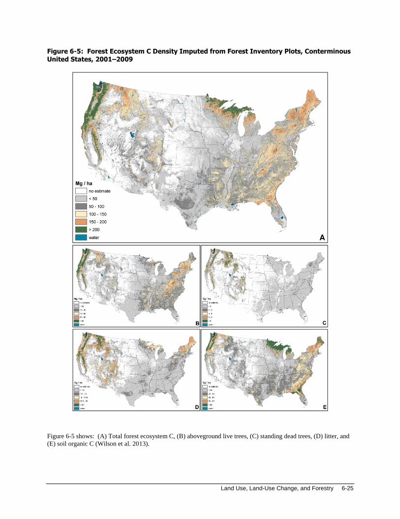
Land Use, Land-Use Change, and Forestry 6-25
Figure 6-5: Forest Ecosystem C Density Imputed from Forest Inventory Plots, Conterminous
United States, 2001–2009
Figure 6-5 shows: (A) Total forest ecosystem C, (B) aboveground live trees, (C) standing dead trees, (D) litter, and
(E) soil organic C (Wilson et al. 2013).

6-26 Inventory of U.S. Greenhouse Gas Emissions and Sinks: 1990–2013
Box 6-3: CO2 Emissions from Forest Fires
As stated previously, the forest inventory approach implicitly accounts for emissions due to disturbances such as
forest fires, because only C remaining in the forest is estimated. Net C stock change is estimated by subtracting
consecutive C stock estimates. A forest fire disturbance removes C from the forest. The inventory data on which
net C stock estimates are based already reflect this C loss. Therefore, estimates of net annual changes in C stocks
for U.S. forest land already account for CO2 emissions from forest fires occurring in the lower 48 states as well as in
the proportion of Alaska’s managed forest land captured in this Inventory. Because it is of interest to quantify the
magnitude of CO2 emissions from fire disturbance, these estimates are highlighted here, using the full extent of
available data. Non-CO2 greenhouse gas emissions from forest fires are also quantified in a separate section below.
The IPCC (2003) methodology and IPCC (2006) default combustion factor for wildfire were employed to estimate
CO2 emissions from forest fires. See the explanation in Annex 3.13 for more details on the methodology used to
estimate CO2 emissions from forest fires. Carbon dioxide emissions for wildfires and prescribed fires in the lower
48 states and wildfires in Alaska in 2013 were estimated to be 77.9 MMT CO2/yr. This amount is masked in the
estimate of net annual forest C stock change for 2013 because this net estimate accounts for the amount sequestered
minus any emissions.
Table 6-11: Estimates of CO2 (MMT/yr) Emissions from Forest Fires for the Lower 48 States
and Alaska
Year
CO2 emitted from
Wildfires in Lower 48
States (MMT/yr)
CO2 emitted from
Prescribed Fires in Lower
48 States (MMT/yr)
CO2 emitted from
Wildfires in Alaska
(MMT/yr)
Total CO2
emitted
(MMT/yr)
1990 28.8 4.9 + 33.7
2005 95.8 14.8 + 110.7
2009 63.5 14.5 + 77.9
2010 49.5 13.9 + 63.4
2011 182.7 12.2 + 194.9
2012 197.7 11.5 + 209.1
2013 66.2 11.7 + 77.9
+ Does not exceed 0.05 MMT CO2 Eq.
Note: These emissions have already been accounted for in the estimates of net annual changes in C stocks, which
account for the amount sequestered minus any emissions.
Methodology and Data Sources
The methodology described herein is consistent with IPCC (2006). Forest ecosystem C stocks and net annual C
stock change were determined according to stock-difference methods, which involved applying C estimation factors
to forest inventory data and interpolating between successive inventory-based estimates of C stocks. Harvested
wood C estimates were based on factors such as the allocation of wood to various primary and end-use products as
well as half-life (the time at which half of the amount placed in use will have been discarded from use) and expected
disposition (e.g., product pool, SWDS, combustion). An overview of the different methodologies and data sources
used to estimate the C in forest ecosystems or harvested wood products is provided here. See Annex 3.13 for details
and additional information related to the methods and data.
Forest Ecosystem Carbon from Forest Inventory
Forest ecosystem stock and flux estimates are based on the stock-difference method and calculations for all
estimates are in units of C. Separate estimates were made for the five IPCC C storage pools described above. All
estimates were based on data collected from the extensive array of permanent forest inventory plots and associated
models (e.g., live tree belowground biomass) in the United States (USDA Forest Service 2013b, 2013c). Carbon
conversion factors were applied at the disaggregated level of each inventory plot and then appropriately expanded to

Land Use, Land-Use Change, and Forestry 6-27
population estimates. A combination of tiers as outlined by IPCC (2006) were used. The Tier 3 biomass C
estimates were calculated from forest inventory tree-level data. The Tier 2 dead organic and soil C estimates were
obtained from empirical or theoretical models using the inventory data. All C conversion factors are specific to
regions or individual states within the United States, which were further classified according to characteristic forest
types within each region.
The first step in developing forest ecosystem estimates is to identify useful inventory data and resolve any
inconsistencies among datasets. Forest inventory data were obtained from the FIA program (Frayer and Furnival
1999, USDA Forest Service 2014b). Inventories include data collected on permanent inventory plots on forest lands
and were organized as separate datasets, each representing a complete inventory, or survey, of an individual state at
a specified time. Many of the more recent annual inventories reported for states are represented as “moving
window” averages, which means that a portion—but not all—of the previous year’s inventory is updated each year
(USDA Forest Service 2014d). Forest C calculations are organized according to these state surveys, and the
frequency of surveys varies by state. All available datasets are identified for each state starting with pre-1990 data,
and all unique surveys are identified for stock and change calculations. Since C stock change is based on
differences between successive surveys within each state, accurate estimates of net C flux thus depend on consistent
representation of forest land between these successive inventories. In order to achieve this consistency from 1990 to
the present, states are sometimes subdivided into sub-state areas where the sum of sub-state inventories produces the
best whole-state representation of C change as discussed in Smith et al. (2010).
The principal FIA datasets employed are freely available for download at USDA Forest Service (2014b) as the
Forest Inventory and Analysis Database (FIADB) Version 6.0 (USDA Forest Service 2014c). However, to achieve
consistent representation (spatial and temporal), three other general sources of past FIA data were included as
necessary. First, older FIA plot- and tree-level data—not in the current FIADB format—are used if available.
Second, Resources Planning Act Assessment (RPA) databases, which are periodic, plot-level only, summaries of
state inventories, are used to provide the data at or before 1990. Finally, the Integrated Database (IDB), which is a
compilation of periodic forest inventory data from the 1990s for California, Oregon, and Washington is used
(Waddell and Hiserote 2005). These IDB data were identified by Heath et al. (2011) as the most appropriate non-
FIADB sources for these states and are included in this Inventory. See USDA Forest Service (2014a) for
information on current and older data as well as additional FIA Program features. A detailed list of the specific
forest inventory data used in this Inventory is included in Annex 3.13.
Modifications to the use of some of the FIADB surveys or subsequent C conversions were initiated for this report.
First, the most-recent FIA population summary (known as an evaluation within the FIADB) was incorporated into
all states’ stock-change calculations which stands in contrast to the approach in previous years where most of the
newest evaluations were already in use, but if the majority of the underlying plots in the most recent population were
also a part of the previous population (i.e., over 50 percent redundant plots) then the recent population was
considered insufficiently unique and not used for calculation. Second, modifications were conducted in coastal
Alaska for developing net annual change estimates (see Annex 3.13) and separating managed versus unmanaged
forest lands in order to exclude C stock and stock-change on unmanaged forest land (IPCC 2006, Ogle et al. in
preparation). This reduced the plots contributing to the Alaska forest C estimates by about 5 percent. A third
modification to the use of the FIADB-defined forest land, introduced this year, was applied to identify plots on
woodland forest types that do not meet the height requirement within the definition of forest land (Oswalt et al.
2014, Coulston et al. in preparation). These plots were identified as “other wooded lands” (i.e., not “forest” within
the FIA forest inventory) and provided as C density information to the grasslands land-use category as the plots
were not a complete inventory of the grassland land-use category in the United States. Finally, a new model
estimating plot level C density of litter was developed and incorporated into the C budget (Domke et al. in
preparation).
Forest C stocks were estimated from inventory data by a collection of conversion factors and models (Birdsey and
Heath 1995, Birdsey and Heath 2001, Heath et al. 2003, Smith et al. 2004, Smith et al. 2006, Woodall et al. 2011a,
Domke et al. 2011, Domke et al. 2012, Domke et al. in preparation), which have been formalized in an FIADB-to-C
calculator (Smith et al. 2010). The conversion factors and model coefficients were categorized by region and forest
type, and forest C stock estimates were calculated from application of these factors at the scale of FIA inventory
plots. The results were estimates of C density (T C per hectare) for six forest ecosystem pools: Live trees, standing
dead trees, understory vegetation, downed dead wood, forest floor, and soil organic matter. The six C pools used in
the FIADB-to-C calculator were aggregated to the five C pools defined by IPCC (2006): Aboveground biomass,
belowground biomass, dead wood, litter, and soil organic matter. The live-tree and understory C were pooled as

6-28 Inventory of U.S. Greenhouse Gas Emissions and Sinks: 1990–2013
biomass, and standing dead trees and downed dead wood were pooled as dead wood, in accordance with IPCC
(2006).
Once plot-level C stocks were calculated as C densities on Forest Land Remaining Forest Land for the five IPCC
(2006) reporting pools, the stocks were expanded to population estimates according to methods appropriate to the
respective inventory data (for example, see Bechtold and Patterson (2005)). These expanded C stock estimates were
summed to state or sub-state total C stocks. Annualized estimates of C stocks were developed by using available
FIA inventory data and interpolating or extrapolating to assign a C stock to each year in the 1990 through 2014 time
series. Flux, or net annual stock change, was estimated by calculating the difference in stocks between two
successive years and applying the appropriate sign convention; net increases in ecosystem C were identified as
negative flux. By convention, inventories were assigned to represent stocks as of January 1 of the inventory year; an
estimate of flux for 1996 required estimates of C stocks for 1996 and 1997, for example. Additional discussion of
the use of FIA inventory data and the C conversion process is in Annex 3.13.
Carbon in Biomass
Live tree C pools include aboveground and belowground (coarse root) biomass of live trees with diameter at
diameter breast height (dbh) of at least 2.54 cm at 1.37 m above the forest floor. Separate estimates were made for
above- and below-ground biomass components. If inventory plots included data on individual trees, tree C was
based on Woodall et al. (2011a), which is also known as the component ratio method (CRM), and is a function of
volume, species, and diameter. An additional component of foliage, which was not explicitly included in Woodall et
al. (2011a), was added to each tree following the same CRM method. Some of the older forest inventory data in use
for these estimates did not provide measurements of individual trees. Examples of these data include plots with
incomplete or missing tree data or the RPA plot-level summaries. The C estimates for these plots were based on
average densities (T C per hectare) obtained from plots of more recent surveys with similar stand characteristics and
location. This applies to less than 5 percent of the forest land inventory-plot-to-C conversions within the 214 state-
level surveys utilized here.
Understory vegetation is a minor component of biomass, which is defined as all biomass of undergrowth plants in a
forest, including woody shrubs and trees less than 2.54 cm dbh. In the current Inventory, it was assumed that 10
percent of total understory C mass is belowground. Estimates of C density were based on information in Birdsey
(1996) and biomass estimates from Jenkins et al. (2003). Understory frequently represented over 1 percent of C in
biomass, but its contribution rarely exceeded 2 percent of the total.
Carbon in Dead Organic Matter
Dead organic matter was initially calculated as three separate pools—standing dead trees, downed dead wood, and
litter—with C stocks estimated from sample data or from models. The standing dead tree C pools include
aboveground and belowground (coarse root) mass and include trees of at least 12.7 cm dbh. Calculations followed
the basic method applied to live trees (Woodall et al. 2011a) with additional modifications to account for decay and
structural loss (Domke et al. 2011, Harmon et al. 2011). Similar to the situation with live tree data, some of the
older forest inventory data did not provide sufficient data on standing dead trees to make accurate population-level
estimates. The C estimates for these plots were based on average densities (T C per hectare) obtained from plots of
more recent surveys with similar stand characteristics and location. This applied to less than 20 percent of the forest
land inventory-plot-to-C conversions within the 214 state-level surveys utilized here. Downed dead wood estimates
are based on measurement of a subset of FIA plots for downed dead wood (Domke et al. 2013, Woodall and
Monleon 2008, Woodall et al. 2013). Downed dead wood is defined as pieces of dead wood greater than 7.5 cm
diameter, at transect intersection, that are not attached to live or standing dead trees. This includes stumps and roots
of harvested trees. To facilitate the downscaling of downed dead wood C estimates from the state-wide population
estimates to individual plots, downed dead wood models specific to regions and forest types within each region are
used. Litter C is the pool of organic C (also known as duff, humus, and fine woody debris) above the mineral soil
and includes woody fragments with diameters of up to 7.5 cm. Estimates are based on Domke et al. (in preparation).
Carbon in Forest Soil
Soil organic C includes all organic material in soil to a depth of 1 meter but excludes the coarse roots of the biomass
or dead wood pools. Estimates of SOC were based on the national STATSGO spatial database (USDA 1991),
which includes region and soil type information. Soil organic C determination was based on the general approach

Land Use, Land-Use Change, and Forestry 6-29
described by Amichev and Galbraith (2004). Links to FIA inventory data were developed with the assistance of the
USDA Forest Service FIA Geospatial Service Center by overlaying FIA forest inventory plots on the soil C map.
This method produced mean SOC densities stratified by region and forest type group. It did not provide separate
estimates for mineral or organic soils but instead weighted their contribution to the overall average based on the
relative amount of each within forest land. Thus, forest SOC is a function of species and location, and net change
also depends on these two factors as total forest area changes. In this respect, SOC provides a country-specific
reference stock for 1990 through the present, but it does not reflect the effects of past land use.
Harvested Wood Carbon
Estimates of the HWP contribution to forest C sinks and emissions (hereafter called “HWP Contribution”) were
based on methods described in Skog (2008) using the WOODCARB II model. These methods are based on IPCC
(2006) guidance for estimating HWP C. IPCC (2006) provides methods that allow for reporting of HWP
Contribution using one of several different accounting approaches: Production, stock change and atmospheric flow,
as well as a default method that assumes there is no change in HWP C stocks (see Annex 3.13 for more details about
each approach). The United States used the production accounting approach to report HWP Contribution. Under
the production approach, C in exported wood was estimated as if it remains in the United States, and C in imported
wood was not included in inventory estimates. Though reported U.S. HWP estimates are based on the production
approach, estimates resulting from use of the two alternative approaches, the stock change and atmospheric flow
approaches, are also presented for comparison (see Annex 3.13). Annual estimates of change were calculated by
tracking the additions to and removals from the pool of products held in end uses (i.e., products in use such as
housing or publications) and the pool of products held in solid waste disposal sites (SWDS). Emissions from HWP
associated with wood biomass energy are not included in this accounting—a net of zero sequestration and emissions
as they are a part of energy accounting (see Chapter 3).
Solidwood products added to pools include lumber and panels. End-use categories for solidwood include single and
multifamily housing, alteration and repair of housing, and other end-uses. There is one product category and one
end-use category for paper. Additions to and removals from pools were tracked beginning in 1900, with the
exception that additions of softwood lumber to housing began in 1800. Solidwood and paper product production
and trade data were taken from USDA Forest Service and other sources (Hair and Ulrich 1963; Hair 1958; USDC
Bureau of Census; 1976; Ulrich, 1985, 1989; Steer 1948; AF&PA 2006a 2006b; Howard 2003, 2007, forthcoming).
Estimates for disposal of products reflected the change over time in the fraction of products discarded to SWDS (as
opposed to burning or recycling) and the fraction of SWDS that were in sanitary landfills versus dumps.
There are five annual HWP variables that were used in varying combinations to estimate HWP Contribution using
any one of the three main approaches listed above. These are:
(1A) annual change of C in wood and paper products in use in the United States,
(1B) annual change of C in wood and paper products in SWDS in the United States,
(2A) annual change of C in wood and paper products in use in the United States and other countries where
the wood came from trees harvested in the United States,
(2B) annual change of C in wood and paper products in SWDS in the United States and other countries
where the wood came from trees harvested in the United States,
(3) C in imports of wood, pulp, and paper to the United States,
(4) C in exports of wood, pulp and paper from the United States, and
(5) C in annual harvest of wood from forests in the United States.
The sum of variables 2A and 2B yielded the estimate for HWP Contribution under the production accounting
approach. A key assumption for estimating these variables was that products exported from the United States and
held in pools in other countries have the same half-lives for products in use, the same percentage of discarded
products going to SWDS, and the same decay rates in SWDS as they would in the United States.

6-30 Inventory of U.S. Greenhouse Gas Emissions and Sinks: 1990–2013
Uncertainty and Time Series Consistency
A quantitative uncertainty analysis placed bounds on current flux for forest ecosystems as well as C in harvested
wood products through Monte Carlo Stochastic Simulation of the Methods described above and probabilistic
sampling of C conversion factors and inventory data. See Annex 3.13 for additional information. The 2013 net
annual change for forest C stocks was estimated to be between -972.9 and -575.9 MMT CO2 Eq. at a 95 percent
confidence level. This includes a range of -900.7 to -505.9 MMT CO2 Eq. for forest ecosystems and -89.9 to -54.0
MMT CO2 Eq. for HWP.
Table 6-12: Approach 2 Quantitative Uncertainty Estimates for Net CO2 Flux from Forest
Land Remaining Forest Land: Changes in Forest C Stocks (MMT CO2 Eq. and Percent)
Source Gas
2013 Flux Estimate Uncertainty Range Relative to Flux Estimatea
(MMT CO2 Eq.) (MMT CO2 Eq.) (%)
Lower
Bound
Upper
Bound
Lower
Bound
Upper
Bound
Forest Ecosystem CO2 (704.9) (900.7) (505.9) −27.8 28.2
Harvested Wood Products CO2 (70.8) (89.9) (54.0) −27.0 23.7
Total Forest CO2 (775.7) (972.9) (575.9) −25.4 25.8
Note: Parentheses indicate negative values or net sequestration. a Range of flux estimates predicted by Monte Carlo stochastic simulation for a 95 percent confidence interval.
Methodological recalculations were applied to the entire time-series to ensure time-series consistency from 1990
through 2013. Details on the emission trends through time are described in more detail in the Methodology section,
above.
QA/QC and Verification
As discussed above, the FIA program has conducted consistent forest surveys based on extensive statistically-based
sampling of most of the forest land in the conterminous United States, dating back to 1952. The FIA program
includes numerous quality assurance and quality control (QA/QC) procedures, including calibration among field
crews, duplicate surveys of some plots, and systematic checking of recorded data. Because of the statistically-based
sampling, the large number of survey plots, and the quality of the data, the survey databases developed by the FIA
program form a strong foundation for C stock estimates. Field sampling protocols, summary data, and detailed
inventory databases are archived and are publicly available on the Internet (USDA Forest Service 2014d).
Many key calculations for estimating current forest C stocks based on FIA data were developed to fill data gaps in
assessing forest C and have been in use for many years to produce national assessments of forest C stocks and stock
changes (see additional discussion and citations in the Methodology section above and in Annex 3.13). General
quality control procedures were used in performing calculations to estimate C stocks based on survey data. For
example, the derived C datasets, which include inventory variables such as areas and volumes, were compared to
standard inventory summaries such as the forest resource statistics of Smith et al. (2009) or selected population
estimates generated from FIADB 6.0, which are available at an FIA internet site (USDA Forest Service 2014b).
Agreement between the C datasets and the original inventories is important to verify accuracy of the data used.
Finally, C stock estimates were compared with previous Inventory report estimates to ensure that any differences
could be explained by either new data or revised calculation methods (see the “Recalculations” discussion, below).
Estimates of the HWP variables and the HWP contribution under the production accounting approach use data from
U.S. Census and USDA Forest Service surveys of production and trade. Factors to convert wood and paper to units
of C are based on estimates by industry and Forest Service published sources. The WOODCARB II model uses
estimation methods suggested by IPCC (2006). Estimates of annual C change in solid wood and paper products in
use were calibrated to meet two independent criteria. The first criterion is that the WOODCARB II model estimate
of C in houses standing in 2001 needs to match an independent estimate of C in housing based on U.S. Census and
USDA Forest Service survey data. Meeting the first criterion resulted in an estimated half-life of about 80 years for
single family housing built in the 1920s, which is confirmed by other U.S. Census data on housing. The second
criterion is that the WOODCARB II model estimate of wood and paper being discarded to SWDS needs to match
EPA estimates of discards each year over the period 1990 to 2000 (EPA 2006). These criteria help reduce

Land Use, Land-Use Change, and Forestry 6-31
uncertainty in estimates of annual change in C in products in use in the United States and, to a lesser degree, reduce
uncertainty in estimates of annual change in C in products made from wood harvested in the United States. In
addition, WOODCARB II landfill decay rates have been validated by ensuring that estimates of CH4 emissions from
landfills based on EPA (2006) data are reasonable in comparison to CH4 estimates based on WOODCARB II
landfill decay rates.
Recalculations Discussion
Forest ecosystem stock and stock-change estimates differ from the previous Inventory (EPA 2014) principally due to
some changes in data and methods (see discussion above in Methodology and in Annex 3.13). The net effect of the
modifications was to slightly reduce net C uptake (i.e., lower sequestration) and C stocks from 1990 to the present.
The influence of the individual modifications on stock and stock-change varied considerably; these were evaluated
to identify the relative sensitivity of totals to each. That is, the analysis identified where the estimates (as in Tables
Table 6-8 through Table 6-10) were most affected by the revised methods incorporated with this report. First, the
collective effects of selecting FIA population estimates and updates to the annual forest inventories for many states
had the effect of decreasing sequestration in early years while increasing after 2005 and had the greatest effect on
determining overall stock-change estimates for 2006 and 2007, but otherwise this modification was a minor
influence. Second, the application of a new managed land definition as part of the land representation analysis (see
Section 6.1) and the subsequent decrease in managed forest lands along coastal Alaska affected that individual
state’s estimates but had minimal effect on C stock estimates for the United States as a whole. Third, the
reallocation of selected woodlands from forest land (i.e., these “other wooded lands” were then classified as
grasslands) had the greatest effect on annualized estimates of forest area throughout the time series. In addition, the
removal of these lands from forest had the greatest effect on total forest stock-change through the early 1990s, yet
the reclassification did tend to decrease sequestration throughout the entire time series. Finally, the revised litter C
estimates generally had a lower influence on stock-change relative to the woodland modification. However, the
revised litter estimates increased sequestration through the 1990s but decreased sequestration over more recent
years. In addition, the change in estimated litter C had the greatest effect on forest ecosystem stocks throughout the
time period.
The estimate of net annual change in HWP C stock and total C stock in HWP were revised upward by small
amounts. The increase in total net annual additions compared to estimates published in 2013 was 2 to 3 percent for
2010 through 2012. This increase was mostly due to changes in the amount of pulpwood used for paper and
composite panel products back to 2003. All the adjustments were made as a result of corrections in the database of
forest products statistics used to prepare the estimates (Howard forthcoming).
Planned Improvements
Reliable estimates of forest C across the diverse ecosystems/industries of the United States require a high level of
investment in both annual monitoring and associated analytical techniques. Development of improved
monitoring/reporting techniques is a continuous process that occurs simultaneously with annual Inventory
submissions. Planned improvements can be broadly assigned to the following categories: Pool estimation
techniques, land use and land-use change, and field inventories.
In an effort to reduce the uncertainty associated with the estimation of individual forest C pools, the empirical data
and associated models for each pool are being evaluated for potential improvement (Woodall 2012). In the 1990
through 2010 Inventory report, the approach to tree volume/biomass estimation was evaluated and refined (Domke
et al. 2012). In the 1990 through 2011 Inventory report, the standing dead tree C model was replaced with a
nationwide inventory and associated empirical estimation techniques (Woodall et al. 2012, Domke et al. 2011,
Harmon et al. 2011). In the 1990 through 2012 Inventory report the downed dead tree C model was refined by
incorporation of a national field inventory of downed dead wood (Woodall et al. 2013, Domke et al. 2013). In the
current Inventory report, the litter C density model was refined with a nearly nationwide field inventory (Domke et
al. in preparation). The exact timing of future pool estimation refinements is dependent on the completion of current
research efforts. Research is underway to use a national inventory of SOC (Woodall et al. 2011b) to refine the
estimation of this pool. It is expected that improvements to SOC estimation will be incorporated into the 1990
through 2015 Inventory report. Components of other pools, such as C in belowground biomass (Russell et al. in
preparation) and understory vegetation (Russell et al. in press), are being explored but may require additional
investment in field inventories before improvements can be realized with Inventory submissions.
6-32 Inventory of U.S. Greenhouse Gas Emissions and Sinks: 1990–2013
Despite the continuing accumulation of new data within the consistent nationwide field inventory of forests that is
measured annually, additional research advances are needed to attain a complete, consistent, and accurate time series
of annual land-use and land-use change matrices from 1990 to the present report year. Lines of research have been
initiated to more fully examine land-use change within the FIA inventory system (see Figure 6-3; Coulston et al. in
review, Wear and Coulston 2014) and bring together disparate sets of land-use information (e.g., forest versus
croplands) that rely on remotely sensed imagery from the 1980s to the present (NASA CMS 2013). These lines of
research are expected to require at least a few years for completion with subsequent time needed for application to
future Inventory submissions.
The foundation of forest C accounting is the annual forest inventory system. The ongoing annual surveys by the
FIA Program are expected to improve the accuracy and precision of forest C estimates as new state surveys become
available (USDA Forest Service 2013b), particularly in western states. Hawaii and U.S. territories will be included
when appropriate forest C data are available (as of July 21, 2014, Hawaii is not yet reporting any data from the
annualized sampling design). In addition, the more intensive sampling of fine woody debris, litter, and SOC on a
subset of FIA plots continues and will substantially improve resolution of C pools (i.e., greater sample intensity;
Westfall et al. 2013) this information becomes available (Woodall et al. 2011b). Increased sample intensity of some
C pools and using annualized sampling data as it becomes available for those states currently not reporting are
planned for future submissions. The USDA Forest Service FIA Program’s forest and wooded land inventories
extend beyond the forest land-use (e.g., woodlands and urban areas), and Inventory-relevant information for these
lands will likely become increasingly available in coming years.
Towards an Accounting of Managed Forest Carbon in Interior Alaska
Given the remote nature and vast expanse of forest across the state of Alaska, consistent inventories of all Alaskan
forest land have never been conducted. Figure 6-6 compares the vast expanse of Alaska to countries in Europe,
which in large part explains the lack of a consistent forest inventory and provides an indication of the extent of any
effort to include an area of this magnitude using the existing forest inventories for the United States. Starting in the
1990s, a forest inventory of south central and southeastern coastal (SCSE) Alaska was initiated following the same
approach applied in the conterminous United States (see Figure 6-7).

Land Use, Land-Use Change, and Forestry 6-33
Figure 6-6: The Size of Alaska Compared to European Countries
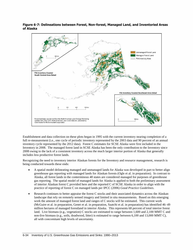
6-34 Inventory of U.S. Greenhouse Gas Emissions and Sinks: 1990–2013
Figure 6-7: Delineations between Forest, Non-forest, Managed Land, and Inventoried Areas
of Alaska
Establishment and data collection on these plots began in 1995 with the current inventory nearing completion of a
full re-measurement (i.e., one cycle of periodic inventory represented by the 2003 data and 90 percent of an annual
inventory cycle represented by the 2012 data). Forest C estimates for SCSE Alaska were first included in the
Inventory in 2008. The managed forest land in SCSE Alaska has been the only contribution to the Inventory since
2008 owing to the lack of a consistent inventory across the much larger interior portion of Alaska that generally
includes less productive forest lands.
Recognizing the need to inventory interior Alaskan forests for the Inventory and resource management, research is
being conducted towards these ends:
A spatial model delineating managed and unmanaged lands for Alaska was developed in part to better align
greenhouse gas reporting with managed lands for Alaskan forests (Ogle et al. in preparation). In contrast to
Alaska, all forest lands in the conterminous 48 states are considered managed for purposes of greenhouse
gas reporting. The spatial model of managed lands for Alaska is applied to both the preliminary assessment
of interior Alaskan forest C provided here and the reported C of SCSE Alaska in order to align with the
practice of reporting of forest C on managed lands per IPCC (2006) Good Practice Guidelines.
Research continues to better appraise the forest C stocks and their associated dynamics across the Alaskan
landscape that rely on remotely sensed imagery and limited in situ measurements. Based on this emerging
work the amount of managed forest land and ranges of C stocks will be estimated. This current work
(McGuire et al. in preparation, Genet et al. in preparation, Saatchi et al. in preparation) has identified 46–49
million hectares of managed forestland in interior Alaska. This represents 68 percent of total interior forest
land. Live biomass (e.g., vegetation) C stocks are estimated to range between 1,600 and 2,100 MMT C and
non-live biomass (e.g., soils, deadwood, litter) is estimated to range between 6,100 and 13,000 MMT C),
all with concomitant high levels of uncertainty.

Land Use, Land-Use Change, and Forestry 6-35
A joint USDA Forest Service-National Aeronautics and Space Administration research effort was
conducted in interior Alaska during the summer of 2014 where high-resolution airborne scanning laser,
hyperspectral, and thermal imagery were collected in a sampling mode over the entire Tanana valley
(135,000 km2). These remotely-sensed data will be combined with a limited number of in situ plot
measurements (100 FIA plots collected within the Tanana Valley State Forest and Tetlin National Wildlife
Refuge) to explore potential application across interior Alaska (NASA CMS 2014). Results from this
research study are expected within a few years.
As preliminary research results suggest that the managed forest C stock may be upwards of 15,000 MMT C or 37
percent of the United States’ managed forest C stock in the current Inventory, care must be given to vet all emerging
research especially in regards to stock change. It is hoped that the managed forest land base in interior Alaska might
be included in future Inventories if: (a) adequate funding resources become available, and (b) research into
combining remotely sensed technologies with in situ measurements (especially of non-vegetation pools) is a success.
Non-CO2 Emissions from Forest Fires Emissions of non-CO2 gases from forest fires were estimated using the default IPCC (2003) methodology
incorporating default IPCC (2006) emissions factors and combustion factor for wildfires. Emissions from this
source in 2013 were estimated to be 5.8 MMT CO2 Eq. of CH4 and 3.8 MMT CO2 Eq. of N2O, as shown in Table
6-13 and Table 6-14. The estimates of non-CO2 emissions from forest fires account for wildfires in the lower 48
states and Alaska as well as prescribed fires in the lower 48 states.
Table 6-13: Estimated Non-CO2 Emissions from Forest Fires (MMT CO2 Eq.) for U.S. Forests
Gas 1990 2005 2009 2010 2011 2012 2013
CH4 2.5 8.3 5.8 4.7 14.6 15.7 5.8
N2O 1.7 5.5 3.8 3.1 9.6 10.3 3.8
Total 4.2 13.8 9.7 7.9 24.2 26.0 9.7
Note: Emissions values are presented in CO2 equivalent mass units using IPCC AR4 GWP
values.
Note: Calculated based on C emission estimates in Changes in Forest Carbon Stocks and
default factors in IPCC (2006).
Table 6-14: Estimated Non-CO2 Emissions from Forest Fires (kt) for U.S. Forests
Gas 1990 2005 2009 2010 2011 2012 2013
CH4 101 332 233 190 584 626 233
N2O 6 18 13 11 32 35 13
Note: Calculated based on C emission estimates in Changes in Forest Carbon Stocks and default
factors in IPCC (2006).
Methodology
The IPCC (2003) Tier 2 default methodology was used to calculate C and CO2 emissions from forest fires.
However, more up-to-date default emission factors from IPCC (2006) were converted into gas-specific emission
ratios and incorporated into the methodology to calculate non-CO2 emissions from C emissions. Estimates of CH4
and N2O emissions were calculated by multiplying the total estimated CO2 emitted from forest burned by the gas-
specific emissions ratios. CO2 emissions were estimated by multiplying total C emitted (Table 6-15) by the C to
CO2 conversion factor of 44/12 and by 92.8 percent, which is the estimated proportion of C emitted as CO2 (Smith
2008a). The equations used to calculate CH4 and N2O emissions were:
CH4 Emissions = (C released) × 92.8% × (44/12) × (CH4 to CO2 emission ratio)
N2O Emissions = (C released) × 92.8% × (44/12) × (N2O to CO2 emission ratio)
Where CH4 to CO2 emission ratio is 0.003 and N2O to CO2 emission ratio is 0.0002. See the explanation in Annex
3.13 for more details on the CH4 and N2O to CO2 emission ratios.

6-36 Inventory of U.S. Greenhouse Gas Emissions and Sinks: 1990–2013
Estimates for C emitted from forest fires are the same estimates used to generate estimates of CO2 presented earlier
in Box 6-3. Estimates for C emitted include emissions from wildfires in both Alaska and the lower 48 states as well
as emissions from prescribed fires in the lower 48 states only (based on expert judgment that prescribed fires only
occur in the lower 48 states) (Smith 2008a). The IPCC (2006) default combustion factor of 0.45 for “all ‘other’
temperate forests” was applied in estimating C emitted from both wildfires and prescribed fires. See the explanation
in Annex 3.13 for more details on the methodology used to estimate C emitted from forest fires.
Table 6-15: Estimated C Released from Forest Fires for U.S. Forests (MMT/yr)
Year C Emitted (MMT/yr)
1990 9.9
2005 32.5
2009 22.9
2010 18.6
2011 57.3
2012 61.5
2013 22.9
Uncertainty and Time-Series Consistency
Non-CO2 gases emitted from forest fires depend on several variables, including: forest area for Alaska and the lower
48 states; average C densities for wildfires in Alaska, wildfires in the lower 48 states, and prescribed fires in the
lower 48 states; emission ratios; and combustion factor values (proportion of biomass consumed by fire). To
quantify the uncertainties for emissions from forest fires, a Monte Carlo (Approach 2) uncertainty analysis was
performed using information about the uncertainty surrounding each of these variables. The results of the Approach
2 quantitative uncertainty analysis are summarized in Table 6-16.
Table 6-16: Approach 2 Quantitative Uncertainty Estimates of Non-CO2 Emissions from Forest Fires in Forest Land Remaining Forest Land (MMT CO2 Eq. and Percent)
Source Gas
2013 Emission Estimate Uncertainty Range Relative to Emission Estimatea
(MMT CO2 Eq.) (MMT CO2 Eq.) (%)
Lower
Bound
Upper
Bound
Lower
Bound
Upper
Bound
Non-CO2 Emissions from
Forest Fires CH4 5.8 1.1 15.2 −80% +161%
Non-CO2 Emissions from
Forest Fires N2O 3.8 1.1 9.2 −71% +139%
a Range of flux estimates predicted by Monte Carlo Stochastic Simulation for a 95 percent confidence interval.
Methodological recalculations were applied to the entire time series to ensure time-series consistency from 1990
through 2013. Details on the emission trends through time are described in more detail in the Methodology section,
above.
QA/QC and Verification
Tier 1 and Tier 2 QA/QC activities were conducted consistent with the U.S. QA/QC plan. Source-specific quality
control measures for forest fires included checking input data, documentation, and calculations to ensure data were
properly handled through the inventory process. The QA/QC analysis did not reveal any inaccuracies or incorrect
input values.
Recalculations Discussion
The current Inventory estimates for 1990 through 2013 were developed according to the methodology used in the
previous Inventory report. However, the FIADB updates discussed in Changes in Forest Carbon Stocks affected
forest C stocks, C density of litter, and total forest area, including the forest area estimates for coastal Alaska, all of

Land Use, Land-Use Change, and Forestry 6-37
which are used to calculate emissions estimates from forest fires. As a result of the FIADB updates, total non-CO2
emissions from forest fires decreased by an average of 14 percent relative to emission estimates in the previous
Inventory report.
For the current Inventory, emission estimates have been revised to reflect the GWPs provided in the IPCC Fourth
Assessment Report (AR4) (IPCC 2007). AR4 GWP values differ slightly from those presented in the IPCC Second
Assessment Report (SAR) (IPCC 1996) (used in the previous inventories) which results in time-series recalculations
for most inventory sources. Under the most recent reporting guidelines (UNFCCC 2014), countries are required to
report using the AR4 GWPs, which reflect an updated understanding of the atmospheric properties of each
greenhouse gas. The GWP of CH4 has increased, leading to an overall increase in CO2-equivalent emissions from
CH4. The GWP of N2O has decreased, leading to a decrease in CO2-equivalent emissions for N2O. The AR4 GWPs
have been applied across the entire time series for consistency. For more information please see the Recalculations
and Improvements Chapter.
The combined effect of the FIADB updates and AR4 GWP values resulted in an average 7 percent decrease in total
non-CO2 emissions from wildfires and prescribed fires over the 1990 to 2012 time series.
Planned Improvements
The default combustion factor of 0.45 from IPCC (2006) was applied in estimating C emitted from both wildfires
and prescribed fires. Additional research into the availability of a combustion factor specific to prescribed fires is
being conducted.
Another area of improvement is to evaluate other methods of obtaining data on forest area burned by replacing ratios
of forest land to land under wildland protection with Monitoring Trends in Burn Severity (MTBS) burn area data.
MTBS data is available from 1984 through a portion of 2013. MTBS burn area data could be used to develop the
national area burned and resulting CO2 and non-CO2 emissions. Additional research is required to determine
appropriate uncertainty inputs for national area burned data derived from MTBS data.
N2O Fluxes from Forest Soils (IPCC Source Category 4A1) Of the synthetic nitrogen (N) fertilizers applied to soils in the United States, no more than one percent is applied to
forest soils. Application rates are similar to those occurring on cropland soils, but in any given year, only a small
proportion of total forested land receives N fertilizer. This is because forests are typically fertilized only twice
during their approximately 40-year growth cycle (once at planting and once midway through their life cycle). Thus,
while the rate of N fertilizer application for the area of forests that receives N fertilizer in any given year is relatively
high, the annual application rate is quite low over the entire forestland area.
N additions to soils result in direct and indirect N2O emissions. Direct emissions occur on-site due to the N
additions. Indirect emissions result from fertilizer N that is transformed and transported to another location in a form
other than N2O (NH3 and NOx volatilization, NO3 leaching and runoff), and later converted into N2O at the off-site
location. The indirect emissions are assigned to forest land because the management activity leading to the
emissions occurred in forest land.
Direct N2O emissions from forest soils in 2013 were 0.3 MMT CO2 Eq. (1 kt), and the indirect emission were 0.1
MMT CO2 Eq. (0.4 kt). Total emissions for 2013 were 0.5 MMT CO2 Eq. (2 kt) and have increased by 455 percent
from 1990 to 2013. Increasing emissions over the time series is a result of greater area of N fertilized pine
plantations in the southeastern United States and Douglas-fir timberland in western Washington and Oregon. Total
forest soil N2O emissions are summarized in Table 6-17.
Table 6-17: N2O Fluxes from Soils in Forest Land Remaining Forest Land (MMT CO2 Eq. and kt N2O)
1990 2005 2009 2010 2011 2012 2013
Direct N2O Fluxes from Soils
MMT CO2 Eq. 0.1 0.3 0.3 0.3 0.3 0.3 0.3
kt N2O + 1 1 1 1 1 1
Indirect N2O Fluxes from Soils
MMT CO2 Eq. + 0.1 0.1 0.1 0.1 0.1 0.1

6-38 Inventory of U.S. Greenhouse Gas Emissions and Sinks: 1990–2013
kt N2O + + + + + + +
Total
MMT CO2 Eq. 0.1 0.5 0.5 0.5 0.5 0.5 0.5
kt N2O + 2 2 2 2 2 2
Note: Emissions values are presented in CO2 equivalent mass units using IPCC AR4 GWP
values.
+ Does not exceed 0.05 MMT CO2 Eq. or 0.5 kt.
Methodology
The IPCC Tier 1 approach was used to estimate N2O from soils within Forest Land Remaining Forest Land.
According to U.S. Forest Service statistics for 1996 (USDA Forest Service 2001), approximately 75 percent of trees
planted were for timber, and about 60 percent of national total harvested forest area is in the southeastern United
States. Although southeastern pine plantations represent the majority of fertilized forests in the United States, this
Inventory also accounted for N fertilizer application to commercial Douglas-fir stands in western Oregon and
Washington. For the Southeast, estimates of direct N2O emissions from fertilizer applications to forests were based
on the area of pine plantations receiving fertilizer in the southeastern United States and estimated application rates
(Albaugh et al. 2007; Fox et al. 2007). Not accounting for fertilizer applied to non-pine plantations is justified
because fertilization is routine for pine forests but rare for hardwoods (Binkley et al. 1995). For each year, the area
of pine receiving N fertilizer was multiplied by the weighted average of the reported range of N fertilization rates
(121 lbs. N per acre). Area data for pine plantations receiving fertilizer in the Southeast were not available for 2005-
2013, so data from 2004 were used for these years. For commercial forests in Oregon and Washington, only
fertilizer applied to Douglas-fir was accounted for, because the vast majority (approximately 95 percent) of the total
fertilizer applied to forests in this region is applied to Douglas-fir (Briggs 2007). Estimates of total Douglas-fir area
and the portion of fertilized area were multiplied to obtain annual area estimates of fertilized Douglas-fir stands.
Similar to the Southeast, data were not available for 2005 through 2013, so data from 2004 were used for these
years. The annual area estimates were multiplied by the typical rate used in this region (200 lbs. N per acre) to
estimate total N applied (Briggs 2007), and the total N applied to forests was multiplied by the IPCC (2006) default
emission factor of 1 percent to estimate direct N2O emissions.
For indirect emissions, the volatilization and leaching/runoff N fractions for forest land were calculated using the
IPCC default factors of 10 percent and 30 percent, respectively. The amount of N volatilized was multiplied by the
IPCC default factor of 1 percent for the portion of volatilized N that is converted to N2O off-site. The amount of N
leached/runoff was multiplied by the IPCC default factor of 0.075 percent for the portion of leached/runoff N that is
converted to N2O off-site The resulting estimates were summed to obtain total indirect emissions.
Uncertainty and Time-Series Consistency
The amount of N2O emitted from forests depends not only on N inputs and fertilized area, but also on a large
number of variables, including organic C availability, oxygen gas partial pressure, soil moisture content, pH,
temperature, and tree planting/harvesting cycles. The effect of the combined interaction of these variables on N2O
flux is complex and highly uncertain. IPCC (2006) does not incorporate any of these variables into the default
methodology, except variation in estimated fertilizer application rates and estimated areas of forested land receiving
N fertilizer. All forest soils are treated equivalently under this methodology. Furthermore, only synthetic N
fertilizers are captured, so applications of organic N fertilizers are not estimated. However, the total quantity of
organic N inputs to soils is included in the Agricultural Soil Management and Settlements Remaining Settlements
sections.
Uncertainties exist in the fertilization rates, annual area of forest lands receiving fertilizer, and the emission factors.
Fertilization rates were assigned a default level30 of uncertainty at ±50 percent, and area receiving fertilizer was
assigned a ±20 percent according to expert knowledge (Binkley 2004). The uncertainty ranges around the 2005
activity data and emission factor input variables were directly applied to the 2013 emissions estimates. IPCC (2006)
provided estimates for the uncertainty associated with direct and indirect N2O emission factor for synthetic N
fertilizer application to soils.
30 Uncertainty is unknown for the fertilization rates so a conservative value of ±50 percent was used in the analysis.

Land Use, Land-Use Change, and Forestry 6-39
Quantitative uncertainty of this source category was estimated using simple error propagation methods (IPCC 2006).
The results of the quantitative uncertainty analysis are summarized in Table 6-18. Direct N2O fluxes from soils
were estimated to be between 0.1 and 1.1 MMT CO2 Eq. at a 95 percent confidence level. This indicates a range of
59 percent below and 211 percent above the 2013 emission estimate of 0.3 MMT CO2 Eq. Indirect N2O emissions in
2013 were between 0.02 and 0.4 MMT CO2 Eq., ranging from 86 percent below to 238 percent above the 2013
emission estimate of 0.11 MMT CO2 Eq.
Table 6-18: Quantitative Uncertainty Estimates of N2O Fluxes from Soils in Forest Land Remaining Forest Land (MMT CO2 Eq. and Percent)
Source Gas
2013 Emission Estimate Uncertainty Range Relative to Emission Estimate
(MMT CO2 Eq.) (MMT CO2 Eq.) (%)
Forest Land Remaining Forest
Land
Lower
Bound
Upper
Bound
Lower
Bound
Upper
Bound
Direct N2O Fluxes from Soils N2O 0.3 0.1 1.1 -59% +211%
Indirect N2O Fluxes from Soils N2O 0.1 0.0 0.4 -86% +238%
Note: These estimates include direct and indirect N2O emissions from N fertilizer additions to both Forest Land
Remaining Forest Land and Land Converted to Forest Land.
Methodological recalculations were applied to the entire time series to ensure time-series consistency from 1990
through 2013. Details on the emission trends through time are described in more detail in the Methodology section,
above.
QA/QC and Verification
The spreadsheet tab containing fertilizer applied to forests and calculations for N2O and uncertainty ranges were
checked and corrected. Linkage errors in the uncertainty calculation for 2013 were found and corrected. The
reported emissions in the NIR were also adjusted accordingly.
Recalculations Discussion
Indirect emissions from forest land were previously reported in Agricultural Soil Management, but are now included
in this source category. Including indirect emissions resulted in a 27 percent increase.
Planned Improvements
Additional data will be compiled to update estimates of forest areas receiving N fertilizer as new reports are made
available. Another improvement is to further disaggregate emissions by state for southeastern pine plantations and
northwestern Douglas-fir forests to estimate soil N2O emission. This improvement is contingent on the availability
of state-level N fertilization data for forest land.
6.3 Land Converted to Forest Land (IPCC Source Category 4A2)
Land-use change is constantly occurring, and areas under a number of differing land-use types are converted to
forest each year, just as forest land is converted to other uses. While the magnitude of these changes is known (see
Table 6-5), research is ongoing to track C across Forest Land Remaining Forest Land and Land Converted to Forest
Land areas. Until such time that reliable and comprehensive estimates of C across these land use and land-use
change categories can be produced, it is not possible to separate CO2 or N2O fluxes on Land Converted to Forest
Land from fluxes on Forest Land Remaining Forest Land at this time.

6-40 Inventory of U.S. Greenhouse Gas Emissions and Sinks: 1990–2013
6.4 Cropland Remaining Cropland (IPCC Source Category 4B1)
Mineral and Organic Soil Carbon Stock Changes Carbon (C) in cropland ecosystems occurs in biomass, dead biomass, and soils. However, C storage in biomass and
dead organic matter is relatively ephemeral, with the exception of C stored in perennial woody crop biomass, such
as citrus groves and apple orchards. Within soils, C is found in organic and inorganic forms of C, but soil organic C
(SOC) is the main source and sink for atmospheric CO2 in most soils. IPCC (2006) recommends reporting changes
in SOC stocks due to agricultural land-use and management activities on both mineral and organic soils.31
Well-drained mineral soils typically contain from 1 to 6 percent organic C by weight, whereas mineral soils with
high water tables for substantial periods during the year may contain significantly more C (NRCS 1999).
Conversion of mineral soils from their native state to agricultural land uses can cause up to half of the SOC to be
lost to the atmosphere due to enhanced microbial decomposition. The rate and ultimate magnitude of C loss
depends on subsequent management practices, climate and soil type (Ogle et al. 2005). Agricultural practices, such
as clearing, drainage, tillage, planting, grazing, crop residue management, fertilization, and flooding, can modify
both organic matter inputs and decomposition, and thereby result in a net flux of C to or from the soil C pool (Parton
et al. 1987, Paustian et al. 1997a, Conant et al. 2001, Ogle et al. 2005). Eventually, the soil can reach a new
equilibrium that reflects a balance between C inputs (e.g., decayed plant matter, roots, and organic amendments such
as manure and crop residues) and C loss through microbial decomposition of organic matter (Paustian et al. 1997b).
Organic soils, also referred to as histosols, include all soils with more than 12 to 20 percent organic C by weight,
depending on clay content (NRCS 1999, Brady and Weil 1999). The organic layer of these soils can be very deep
(i.e., several meters), and form under inundated conditions that results in minimal decomposition of plant residues.
When organic soils are prepared for crop production, they are drained and tilled, leading to aeration of the soil that
accelerates both the decomposition rate and CO2 emissions. Due to the depth and richness of the organic layers, C
loss from drained organic soils can continue over long periods of time, which varies depending on climate and
composition (i.e., decomposability) of the organic matter (Armentano and Menges 1986). Due to deeper drainage
and more intensive management practices, the use of organic soils for annual crop production leads to higher C loss
rates than drainage of organic soils in grassland or forests (IPCC 2006).
Cropland Remaining Cropland includes all cropland in an Inventory year that has been used as cropland for the
previous 20 years according to the 2007 USDA National Resources Inventory (NRI) land-use survey (USDA-NRCS
2009).32 The inventory includes all privately-owned croplands in the conterminous United States and Hawaii, but
does not include the 1 to 1.5 million hectares of Cropland Remaining Cropland (less than 1 percent of the total
cropland area in the United States) on federal lands between 1990 and 2013. In addition, approximately 28,700
hectares of cropland in Alaska are not included in this Inventory. This leads to a discrepancy between the total
amount of managed area in Cropland Remaining Cropland (see Section 6.1) and the cropland area included in the
Inventory. Improvements are underway to include croplands in Alaska and federal lands as part of future C
inventories.
CO2 emissions and removals33 due to changes in mineral soil C stocks are estimated using a Tier 3 approach for the
majority of annual crops (Ogle et al. 2010). A Tier 2 IPCC method is used for the remaining crops not included in
the Tier 3 method (i.e., vegetables, tobacco, perennial/horticultural crops, and rice) (Ogle et al. 2003, 2006). In
addition, a Tier 2 method is used for very gravelly, cobbly, or shaley soils (i.e., classified as soils that have greater
than 35 percent of soil volume comprised of gravel, cobbles, or shale) and for additional changes in mineral soil C
31 CO2 emissions associated with liming are also estimated but are included in a separate section of the report. 32 NRI points were classified according to land-use history records starting in 1982 when the NRI survey began, and
consequently the classifications were based on less than 20 years from 1990 to 2001. 33 Note that removals occur through uptake of CO2 into crop and forage biomass that is later incorporated into soil C pools.

Land Use, Land-Use Change, and Forestry 6-41
stocks that were not addressed with the Tier 3 approach (i.e., change in C stocks after 2007 due to Conservation
Reserve Program enrollment). Emissions from organic soils are estimated using a Tier 2 IPCC method.
Land-use and land management of mineral soils was the largest contributor to total net C stock change, especially in
the early part of the time series (see Table 6-19 and Table 6-20). (Note: Estimates after 2007 are based on NRI data
from 2007 and therefore do not fully reflect changes occurring in the latter part of the time series). In 2013, mineral
soils were estimated to remove 45.6 MMT CO2 Eq. (12.4 MMT C). This rate of C storage in mineral soils
represented about a 49 percent decrease in the rate since the initial reporting year of 1990. Emissions from organic
soils were 22.1 MMT CO2 Eq. (6.0 MMT C) in 2013, which is an 8 percent decrease compared to 1990. In total,
United States agricultural soils in Cropland Remaining Cropland sequestered approximately 23.4 MMT CO2 Eq.
(6.4 MMT C) in 2013.
Table 6-19: Net CO2 Flux from Soil C Stock Changes in Cropland Remaining Cropland (MMT
CO2 Eq.)
Soil Type 1990 2005 2009 2010 2011 2012 2013
Mineral Soils (89.2) (50.4) (49.6) (48.0) (47.9) (47.1) (45.6)
Organic Soils 24.0 22.4 22.1 22.1 22.1 22.1 22.1
Total Net Flux (65.2) (28.0) (27.5) (25.9) (25.8) (25.0) (23.4)
Note: Totals may not sum due to independent rounding. Parentheses indicate net sequestration.
Note: Estimates after 2007 are based on NRI data from 2007 and therefore may not fully reflect
changes occurring in the latter part of the time series
Table 6-20: Net CO2 Flux from Soil C Stock Changes in Cropland Remaining Cropland (MMT C)
Soil Type 1990 2005 2009 2010 2011 2012 2013
Mineral Soils (24.3) (13.8) (13.5) (13.1) (13.1) (12.9) (12.4)
Organic Soils 6.5 6.1 6.0 6.0 6.0 6.0 6.0
Total Net Flux (17.8) (7.6) (7.5) (7.1) (7.0) (6.8) (6.4)
Note: Totals may not sum due to independent rounding. Parentheses indicate net
sequestration.
Note: Estimates after 2007 are based on NRI data from 2007 and therefore may not
fully reflect changes occurring in the latter part of the time series
The major cause of the reduction in soil C accumulation over the time series (i.e., 2013 is 49 percent less than 1990)
is the decline in annual cropland enrolled in the Conservation Reserve Program (CRP)34 which was initiated in 1985
(Jones et al., in prep). For example, over 2 million hectares of land in the CRP were returned to agricultural
production, during the last 5 years resulting in a loss of soil C. However, positive increases in C stocks continue on
the nearly 11 million hectares of land currently enrolled in the CRP, as well as from intensification of crop
production by limiting the use of bare-summer fallow in semi-arid regions, increased hay production, and adoption
of conservation tillage (i.e., reduced- and no-till practices).
The spatial variability in the 2013 annual CO2 flux is displayed in Figure 6-8 and Figure 6-9 for C stock changes in
mineral and organic soils, respectively. The highest rates of net C accumulation in mineral soils occurred in the
Midwest, which is the region with the largest amounts of conservation tillage, with the next highest rates of
accumulation in the South-central and Northwest regions of the United States. The regions with the highest rates of
emissions from organic soils occur in the Southeastern Coastal Region (particularly Florida), upper Midwest and
34 The Conservation Reserve Program (CRP) is a land conservation program administered by the Farm Service Agency (FSA).
In exchange for a yearly rental payment, farmers enrolled in the program agree to remove environmentally sensitive land from
agricultural production and plant species that will improve environmental health and quality. Contracts for land enrolled in CRP
are 10-15 years in length. The long-term goal of the program is to re-establish valuable land cover to help improve water quality,
prevent soil erosion, and reduce loss of wildlife habitat.

6-42 Inventory of U.S. Greenhouse Gas Emissions and Sinks: 1990–2013
Northeast surrounding the Great Lakes, and the Pacific Coast (particularly California), which coincides with largest
concentrations of organic soils in the United States that are used for agricultural production.
Figure 6-8: Total Net Annual CO2 Flux for Mineral Soils under Agricultural Management within States, 2013, Cropland Remaining Cropland

Land Use, Land-Use Change, and Forestry 6-43
Figure 6-9: Total Net Annual CO2 Flux for Organic Soils under Agricultural Management
within States, 2013, Cropland Remaining Cropland
Methodology
The following section includes a description of the methodology used to estimate changes in soil C stocks for
Cropland Remaining Cropland, including (1) agricultural land-use and management activities on mineral soils; and
(2) agricultural land-use and management activities on organic soils.
Soil C stock changes were estimated for Cropland Remaining Cropland (as well as agricultural land falling into the
IPCC categories Land Converted to Cropland, Grassland Remaining Grassland, and Land Converted to Grassland)
according to land-use histories recorded in the USDA NRI survey (USDA-NRCS 2009). The NRI is a statistically-
based sample of all non-federal land, and includes approximately 529,558 points in agricultural land for the
conterminous United States and Hawaii.35 Each point is associated with an “expansion factor” that allows scaling of
C stock changes from NRI points to the entire country (i.e., each expansion factor represents the amount of area with
the same land-use/management history as the sample point). Land-use and some management information (e.g.,
crop type, soil attributes, and irrigation) were originally collected for each NRI point on a 5-year cycle beginning in
1982. For cropland, data were collected for 4 out of 5 years in the cycle (i.e., 1979-1982, 1984-1987, 1989-1992,
T
35T NRI points were classified as agricultural if under grassland or cropland management between 1990 and 2007.

6-44 Inventory of U.S. Greenhouse Gas Emissions and Sinks: 1990–2013
and 1994-1997). In 1998, the NRI program began collecting annual data, and data are currently available through
2010 (USDA-NRCS, 2013) although this Inventory only uses NRI data through 2007 because newer data were not
made available in time to incorporate the additional years into this Inventory. NRI points were classified as
Cropland Remaining Cropland in a given year between 1990 and 2007 if the land use had been cropland for 20
years.36 Cropland includes all land used to produce food and fiber, or forage that is harvested and used as feed (e.g.,
hay and silage), in addition to cropland that has been enrolled in the CRP (i.e., considered reserve cropland).
Mineral Soil Carbon Stock Changes
An IPCC Tier 3 model-based approach (Ogle et al. 2010) was applied to estimate C stock changes for mineral soils
on the majority of land that is used to produce annual crops in the United States. These crops include alfalfa hay,
barley, corn, cotton, dry beans, grass hay, grass-clover hay, oats, onions, peanuts, potatoes, rice, sorghum, soybeans,
sugar beets, sunflowers, tomatoes, and wheat. The model-based approach uses the DAYCENT biogeochemical
model (Parton et al. 1998; Del Grosso et al. 2001, 2011) to estimate soil C stock changes and soil nitrous oxide
emissions from agricultural soil management. Carbon and N dynamics are linked in plant-soil systems through the
biogeochemical processes of microbial decomposition and plant production (McGill and Cole 1981). Coupling the
two source categories (i.e., agricultural soil C and N2O) in a single inventory analysis ensures that there is a
consistent treatment of the processes and interactions between C and N cycling in soils.
The remaining crops on mineral soils were estimated using an IPCC Tier 2 method (Ogle et al. 2003), including
some vegetables, tobacco, perennial/horticultural crops, and crops that are rotated with these crops. The Tier 2
method was also used for very gravelly, cobbly, or shaley soils (greater than 35 percent by volume). Mineral SOC
stocks were estimated using a Tier 2 method for these areas because the DAYCENT model, which is used for the
Tier 3 method, has not been fully tested for estimating C stock changes associated with these crops and rotations, as
well as cobbly, gravelly, or shaley soils. An additional stock change calculation was estimated for mineral soils
using Tier 2 emission factors to account for enrollment patterns in the CRP after 2007, which was not addressed by
the Tier 3 method.
Further elaboration on the methodology and data used to estimate stock changes from mineral soils are described
below and in Annex 3.12.
Tier 3 Approach
Mineral SOC stocks and stock changes were estimated using the DAYCENT biogeochemical37 model (Parton et al.
1998; Del Grosso et al. 2001, 2011), which simulates cycling of C, N and other nutrients in cropland, grassland,
forest, and savanna ecosystems. The DAYCENT model utilizes the soil C modeling framework developed in the
Century model (Parton et al. 1987, 1988, 1994; Metherell et al. 1993), but has been refined to simulate dynamics at a
daily time-step. Crop production is simulated with NASA-CASA production algorithm (Potter et al.1993, Potter et
al. 2007) using the MODIS Enhanced Vegetation Index (EVI) products, MOD13Q1 and MYD13Q1, with a pixel
resolution of 250 m. A prediction algorithm was developed to estimate EVI (Gurung et al. 2009) for gap-filling
during years over the inventory time series when EVI data were not available (e.g., data from the MODIS sensor
were only available after 2000 following the launch of the Aqua and Terra Satellites). The modeling approach uses
daily weather data as an input, along with information about soil physical properties. Input data on land use and
management are specified at a daily resolution and include land-use type, crop/forage type, and management
activities (e.g., planting, harvesting, fertilization, manure amendments, tillage, irrigation, residue removal, grazing,
and fire). The model simulates net primary productivity and C additions to soil, soil temperature, and water
dynamics, in addition to turnover, stabilization, and mineralization of soil organic matter C and nutrients (N, P, K,
S). This method is more accurate than the Tier 1 and 2 approaches provided by the IPCC (2006) because the
simulation model treats changes as continuous over time as opposed to the simplified discrete changes represented
in the default method (see Box 6-4 X for additional information).
36 NRI points were classified according to land-use history records starting in 1982 when the NRI survey began. Therefore, the
classification prior to 2002 was based on less than 20 years of recorded land-use history for the time series. 37 Biogeochemical cycles are the flow of chemical elements and compounds between living organisms and the physical
environment

Land Use, Land-Use Change, and Forestry 6-45
Box 6-4: Tier 3 Approach for Soil C Stocks Compared to Tier 1 or 2 Approaches
A Tier 3 model-based approach is used to estimate soil C stock changes on the majority of agricultural land on
mineral soils. This approach results in a more complete accounting of soil C stock changes and entails several
fundamental differences from the IPCC Tier 1 or 2 methods, as described below.
(1) The IPCC Tier 1 and 2 methods are simplified and classify land areas into discrete categories based on
highly aggregated information about climate (six regions), soil (seven types), and management (eleven
management systems) in the United States. In contrast, in the Tier 3 model, the same variables (i.e.
climate, soils, and management systems) are represented in considerably more detail both temporally and
spatially, and exhibit multi-dimensional interactions through the more complex model structure.
(2) The IPCC Tier 1 and 2 methods have a simplified spatial resolution, where, in the United States, data is
aggregated to climate and soil regions. In contrast, the Tier 3 model uses more than 300,000 individual NRI
point locations in individual fields.
(3) The IPCC Tier 1 and 2 methods use simplified equilibrium step changes for changes in carbon emissions.
In contrast, the Tier 3 approach simulates a continuous time period. More specifically, the DAYCENT
model (i.e., daily time-step version of the Century model) simulates soil C dynamics (and CO2 emissions
and uptake) on a daily time step based on C emissions and removals from plant production and
decomposition processes. These changes in soil C stocks are influenced by multiple sources that affect
primary production and decomposition, including changes in land use and management, weather variability
and secondary feedbacks between management activities, climate, and soils.
Historical land-use patterns are simulated with DAYCENT based on the 2007 USDA NRI survey, in addition to
information on irrigation (USDA-NRCS 2009). Additional sources of activity data were used to supplement the
land-use information from NRI. The Conservation Technology Information Center (CTIC 2004) provided annual
data on tillage activity at the county level since 1989, with adjustments for long-term adoption of no-till agriculture
(Towery 2001). Information on fertilizer use and rates by crop type for different regions of the United States were
obtained primarily from the USDA Economic Research Service Cropping Practices Survey (USDA-ERS 1997,
2011) with additional data from other sources, including the National Agricultural Statistics Service (NASS 1992,
1999, 2004). Frequency and rates of manure application to cropland during 1997 were estimated from data
compiled by the USDA Natural Resources Conservation Service (Edmonds et al. 2003), and then adjusted using
county-level estimates of manure available for application in other years. Specifically, county-scale ratios of
manure available for application to soils in other years relative to 1997 were used to adjust the area amended with
manure (see Annex 3.12 for further details). Greater availability of managed manure N relative to 1997 was, thus,
assumed to increase the area amended with manure, while reduced availability of manure N relative to 1997 was
assumed to reduce the amended area. Data on the county-level N available for application were estimated for
managed systems based on the total amount of N excreted in manure minus N losses during storage and transport,
and including the addition of N from bedding materials. Nitrogen losses include direct N2O emissions, volatilization
of ammonia and NOx, runoff and leaching, and poultry manure used as a feed supplement. For unmanaged systems,
it is assumed that no N losses or additions occur prior to the application of manure to the soil. More information on
livestock manure production is available in the Manure Management, Section 5.2, and Annex 3.11.
Daily weather data were used as an input in the model simulations based on gridded data at a 32 km scale from the
North America Regional Reanalysis Product (NARR) (Mesinger et al. 2006). Soil attributes were obtained from the
Soil Survey Geographic Database (SSURGO) (Soil Survey Staff 2005). The C dynamics at each NRI point was
simulated 100 times as part of the uncertainty analysis, yielding a total of over 18 million simulation runs for the
analysis. Uncertainty in the C stock estimates from DAYCENT associated with parameterization and model
algorithms were adjusted using a structural uncertainty estimator accounting for uncertainty in model algorithms and
parameter values (Ogle et al. 2007, 2010). Carbon stocks and 95 percent confidence intervals were estimated for
each year between 1990 and 2007, but C stock changes from 2008 to 2013 were assumed to be similar to 2007 for
this Inventory due to a lack of activity data for these years. (Future Inventories will be updated with new activity
data and the time series will be recalculated; see Planned Improvements section).

6-46 Inventory of U.S. Greenhouse Gas Emissions and Sinks: 1990–2013
Tier 2 Approach
In the IPCC Tier 2 method, data on climate, soil types, land-use, and land management activity were used to classify
land area and apply appropriate stock change factors (Ogle et al. 2003, 2006). Major Land Resource Areas
(MLRAs) formed the base spatial unit for conducting the Tier 2 analysis. MLRAs represent a geographic unit with
relatively similar soils, climate, water resources, and land uses (NRCS 1981). MLRAs were classified into climate
regions according to the IPCC categories using the PRISM climate database of Daly et al. (1994), and the factors
were assigned based on the land management systems in the MLRA in addition to the climate and soil types.
Reference C stocks were estimated using the National Soil Survey Characterization Database (NRCS 1997) with
cultivated cropland as the reference condition, rather than native vegetation as used in IPCC (2006). Soil
measurements under agricultural management are much more common and easily identified in the National Soil
Survey Characterization Database (NRCS 1997) than are soils under a native condition, and therefore cultivated
cropland provided a more robust sample for estimating the reference condition.
U.S.-specific stock change factors were derived from published literature to determine the impact of management
practices on SOC storage (Ogle et al. 2003, Ogle et al. 2006). The factors include changes in tillage, cropping
rotations, intensification, and land-use change between cultivated and uncultivated conditions. U.S. factors
associated with organic matter amendments were not estimated due to an insufficient number of studies in the
United States to analyze the impacts. Instead, factors from IPCC (2003) were used to estimate the effect of those
activities.
Activity data were primarily based on the historical land-use/management patterns recorded in the 2007 NRI
(USDA-NRCS 2009). Each NRI point was classified by land use, soil type, climate region (using PRISM data, Daly
et al. 1994) and management condition. Classification of cropland area by tillage practice was based on data from
the Conservation Technology Information Center (CTIC 2004, Towery 2001) as described above. Activity data on
wetland restoration of Conservation Reserve Program land were obtained from Euliss and Gleason (2002). Manure
N amendments over the inventory time period were based on application rates and areas amended with manure N
from Edmonds et al. (2003), in addition to the managed manure production data discussed in the methodology
subsection for the Tier 3 analysis.
Combining information from these data sources, SOC stocks for mineral soils were estimated 50,000 times for 1982,
1992, 1997, 2002 and 2007, using a Monte Carlo stochastic simulation approach and probability distribution
functions for U.S.-specific stock change factors, reference C stocks, and land-use activity data (Ogle et al. 2002,
Ogle et al. 2003, Ogle et al. 2006). The annual C flux for 1990 through 1992 was determined by calculating the
average annual change in stocks between 1982 and 1992; annual C flux for 1993 through 1997 was determined by
calculating the average annual change in stocks between 1992 and 1997; annual C flux for 1998 through 2002 was
determined by calculating the average annual change in stocks between 1998 and 2002; and annual C flux from
2003 through 2013 was determined by calculating the average annual change in stocks between 2003 and 2007.
Additional Mineral C Stock Change
Annual C flux estimates for mineral soils between 2008 and 2013 were adjusted to account for additional C stock
changes associated with gains or losses in soil C after 2007 due to changes in CRP enrollment (USDA-FSA 2013).
The change in enrollment relative to 2007 was based on data from USDA-FSA (2013) for 2008 through 2013. The
differences in mineral soil areas were multiplied by 0.5 metric tons C per hectare per year to estimate the net effect
on soil C stocks. The stock change rate is based on country-specific factors and the IPCC default method (see
Annex 3.12 for further discussion).
Organic Soil Carbon Stock Changes
Annual C emissions from drained organic soils in Cropland Remaining Cropland were estimated using the Tier 2
method provided in IPCC (2006), with U.S.-specific C loss rates (Ogle et al. 2003) rather than default IPCC rates.
The final estimates included a measure of uncertainty as determined from the Monte Carlo Stochastic Simulation
with 50,000 iterations. Emissions were based on the annual data from 1990 to 2007 for Cropland Remaining
Cropland areas in the 2007 NRI (USDA-NRCS 2009). The annual emissions estimated for 2007 were applied to

Land Use, Land-Use Change, and Forestry 6-47
2007 through 2013. (Future inventories will be updated with new activity data and the time series will be
recalculated; see Planned Improvements section).
Uncertainty and Time-Series Consistency
Uncertainty associated with the Cropland Remaining Cropland land-use category was addressed for changes in
agricultural soil C stocks (including both mineral and organic soils). Uncertainty estimates are presented in Table
6-21 for each subsource (mineral soil C stocks and organic soil C stocks) and the method that was used in the
inventory analysis (i.e., Tier 2 and Tier 3). Uncertainty for the portions of the Inventory estimated with Tier 2 and 3
approaches was derived using a Monte Carlo approach (see Annex 3.12 for further discussion). Uncertainty
estimates from each approach were combined using the error propagation equation in accordance with IPCC (2006).
The combined uncertainty was calculated by taking the square root of the sum of the squares of the standard
deviations of the uncertain quantities. The combined uncertainty for soil C stocks in Cropland Remaining Cropland
ranged from 152 percent below to 154 percent above the 2013 stock change estimate of -23.4 MMT CO2 Eq.
Table 6-21: Approach 2 Quantitative Uncertainty Estimates for Soil C Stock Changes
occurring within Cropland Remaining Cropland (MMT CO2 Eq. and Percent)
Source
2013 Flux Estimate
(MMT CO2 Eq.)
Uncertainty Range Relative to Flux Estimatea
(MMT CO2 Eq.) (%)
Lower
Bound
Upper
Bound
Lower
Bound
Upper
Bound
Mineral Soil C Stocks: Cropland Remaining
Cropland, Tier 3 Inventory Methodology (49.3) (83.7) (14.9) -70% 70%
Mineral Soil C Stocks: Cropland Remaining
Cropland, Tier 2 Inventory Methodology (2.8) (5.1) (0.9) -80% 68%
Mineral Soil C Stocks: Cropland Remaining
Cropland (Change in CRP enrollment relative
to 2003)
6.6 3.3 9.9 -50% 50%
Organic Soil C Stocks: Cropland Remaining
Cropland, Tier 2 Inventory Methodology 22.1 14.0 32.5 -37% 47%
Combined Uncertainty for Flux associated
with Agricultural Soil Carbon Stock
Change in Cropland Remaining Cropland
(23.4) (59.0) 12.7 -152% 154%
a Range of flux estimates predicted by Monte Carlo Stochastic Simulation for a 95 percent confidence interval.
Note: Parentheses indicate net sequestration.
Uncertainty is also associated with lack of reporting of agricultural biomass and litter C stock changes. Biomass C
stock changes are likely minor in perennial crops, such as orchards and nut plantations, given the small amount of
change in land used to produce these commodities in the United States. In contrast, agroforestry practices, such as
shelterbelts, riparian forests and intercropping with trees, may have led to significant changes in biomass C stocks,
at least in some regions of the United States, but there are currently no datasets to evaluate the trends. Changes in
litter C stocks are also assumed to be negligible in croplands over annual time frames, although there are certainly
significant changes at sub-annual time scales across seasons. However, this trend may change in the future,
particularly if crop residue becomes a viable feedstock for bioenergy production.
Methodological recalculations were applied to the entire time series to ensure time-series consistency from 1990
through 2013. Details on the emission trends through time are described in more detail in the Methodology section,
above.
QA/QC and Verification
Quality control measures included checking input data, model scripts, and results to ensure data were properly
handled throughout the inventory process. Inventory reporting forms and text were reviewed and revised as needed
to correct transcription errors. As discussed in the uncertainty section, results were compared to field measurements,
and a statistical relationship was developed to assess uncertainties in the model’s predictive capability. The
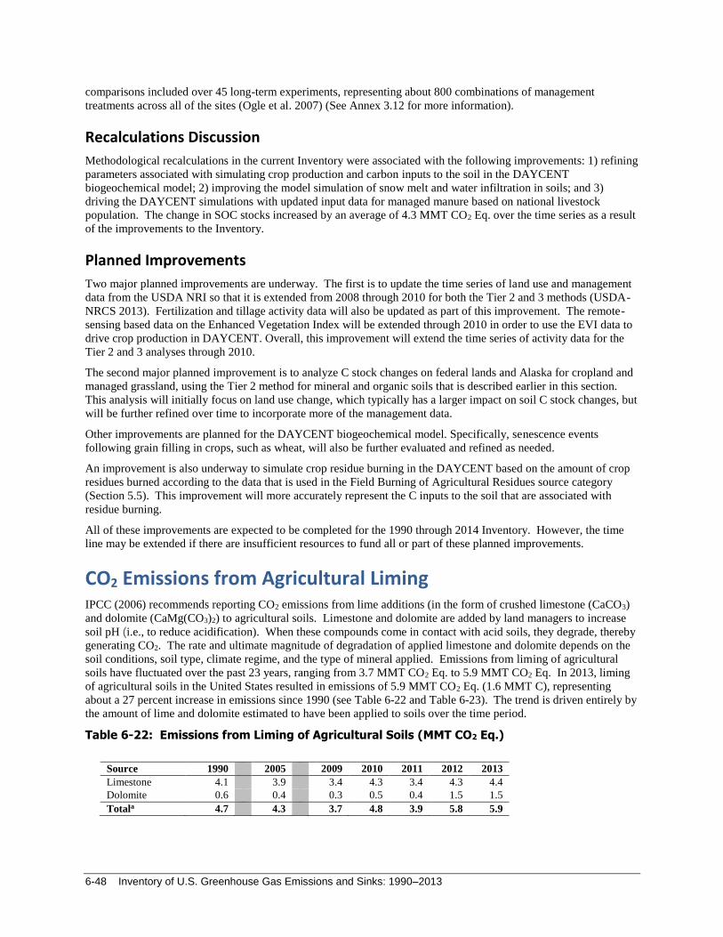
6-48 Inventory of U.S. Greenhouse Gas Emissions and Sinks: 1990–2013
comparisons included over 45 long-term experiments, representing about 800 combinations of management
treatments across all of the sites (Ogle et al. 2007) (See Annex 3.12 for more information).
Recalculations Discussion
Methodological recalculations in the current Inventory were associated with the following improvements: 1) refining
parameters associated with simulating crop production and carbon inputs to the soil in the DAYCENT
biogeochemical model; 2) improving the model simulation of snow melt and water infiltration in soils; and 3)
driving the DAYCENT simulations with updated input data for managed manure based on national livestock
population. The change in SOC stocks increased by an average of 4.3 MMT CO2 Eq. over the time series as a result
of the improvements to the Inventory.
Planned Improvements
Two major planned improvements are underway. The first is to update the time series of land use and management
data from the USDA NRI so that it is extended from 2008 through 2010 for both the Tier 2 and 3 methods (USDA-
NRCS 2013). Fertilization and tillage activity data will also be updated as part of this improvement. The remote-
sensing based data on the Enhanced Vegetation Index will be extended through 2010 in order to use the EVI data to
drive crop production in DAYCENT. Overall, this improvement will extend the time series of activity data for the
Tier 2 and 3 analyses through 2010.
The second major planned improvement is to analyze C stock changes on federal lands and Alaska for cropland and
managed grassland, using the Tier 2 method for mineral and organic soils that is described earlier in this section.
This analysis will initially focus on land use change, which typically has a larger impact on soil C stock changes, but
will be further refined over time to incorporate more of the management data.
Other improvements are planned for the DAYCENT biogeochemical model. Specifically, senescence events
following grain filling in crops, such as wheat, will also be further evaluated and refined as needed.
An improvement is also underway to simulate crop residue burning in the DAYCENT based on the amount of crop
residues burned according to the data that is used in the Field Burning of Agricultural Residues source category
(Section 5.5). This improvement will more accurately represent the C inputs to the soil that are associated with
residue burning.
All of these improvements are expected to be completed for the 1990 through 2014 Inventory. However, the time
line may be extended if there are insufficient resources to fund all or part of these planned improvements.
CO2 Emissions from Agricultural Liming IPCC (2006) recommends reporting CO2 emissions from lime additions (in the form of crushed limestone (CaCO3)
and dolomite (CaMg(CO3)2) to agricultural soils. Limestone and dolomite are added by land managers to increase
soil pH (i.e., to reduce acidification). When these compounds come in contact with acid soils, they degrade, thereby
generating CO2. The rate and ultimate magnitude of degradation of applied limestone and dolomite depends on the
soil conditions, soil type, climate regime, and the type of mineral applied. Emissions from liming of agricultural
soils have fluctuated over the past 23 years, ranging from 3.7 MMT CO2 Eq. to 5.9 MMT CO2 Eq. In 2013, liming
of agricultural soils in the United States resulted in emissions of 5.9 MMT CO2 Eq. (1.6 MMT C), representing
about a 27 percent increase in emissions since 1990 (see Table 6-22 and Table 6-23). The trend is driven entirely by
the amount of lime and dolomite estimated to have been applied to soils over the time period.
Table 6-22: Emissions from Liming of Agricultural Soils (MMT CO2 Eq.)
Source 1990 2005 2009 2010 2011 2012 2013
Limestone 4.1 3.9 3.4 4.3 3.4 4.3 4.4
Dolomite 0.6 0.4 0.3 0.5 0.4 1.5 1.5
Totala 4.7 4.3 3.7 4.8 3.9 5.8 5.9

Land Use, Land-Use Change, and Forestry 6-49
a Also includes emissions from liming on Land Converted to Cropland, Grassland
Remaining Grassland, Land Converted to Grassland, and Settlements Remaining
Settlements as it is not currently possible to apportion the data by land-use category.
Note: Totals may not sum due to independent rounding.
Table 6-23: Emissions from Liming of Agricultural Soils (MMT C)
Source 1990 2005 2009 2010 2011 2012 2013
Limestone 1.1 1.1 0.9 1.2 0.9 1.2 1.2
Dolomite 0.2 0.1 0.1 0.1 0.1 0.4 0.4
Totala 1.3 1.2 1.0 1.3 1.1 1.6 1.6
a Also includes emissions from liming on Land Converted to Cropland, Grassland
Remaining Grassland, Land Converted to Grassland, and Settlements Remaining Settlements
as it is not currently possible to apportion the data by land-use category.
Note: Totals may not sum due to independent rounding.
Methodology
CO2 emissions from degradation of limestone and dolomite applied to agricultural soils were estimated using a Tier
2 methodology consistent with IPCC (2006). The annual amounts of limestone and dolomite applied (see Table
6-24) were multiplied by CO2 emission factors from West and McBride (2005). These emission factors (0.059
metric ton C/metric ton limestone, 0.064 metric ton C/metric ton dolomite) are lower than the IPCC default emission
factors because they account for the portion of agricultural lime that may leach through the soil and travel by rivers
to the ocean (West and McBride 2005). This analysis of lime dissolution is based on liming occurring in the
Mississippi River basin, where the vast majority of all U.S. liming takes place (West 2008). U.S. liming that does
not occur in the Mississippi River basin tends to occur under similar soil and rainfall regimes, and, thus, the
emission factor is appropriate for use across the United States (West 2008). The annual application rates of
limestone and dolomite were derived from estimates and industry statistics provided in the Minerals Yearbook and
Mineral Industry Surveys (Tepordei 1993 through 2006; Willett 2007a, 2007b, 2009, 2010, 2011a, 2011b, 2013a and
2014; USGS 2008 through 2014). To develop these data, the U.S. Geological Survey (USGS; U.S. Bureau of Mines
prior to 1997) obtained production and use information by surveying crushed stone manufacturers. Because some
manufacturers were reluctant to provide information, the estimates of total crushed limestone and dolomite
production and use were divided into three components: (1) production by end-use, as reported by manufacturers
(i.e., “specified” production); (2) production reported by manufacturers without end-uses specified (i.e.,
“unspecified” production); and (3) estimated additional production by manufacturers who did not respond to the
survey (i.e., “estimated” production).
Box 6-5: Comparison of the Tier 2 U.S. Inventory Approach and IPCC (2006) Default Approach
Emissions from liming of agricultural soils were estimated using a Tier 2 methodology based on liming emission
factors specific to the United States that are lower than the IPCC (2006) emission default factors, and are specific to
U.S. soil conditions under which liming occurs. For example, as described previously, most liming in the United
States occurs in the Mississippi River basin, or in areas that have similar soil and rainfall regimes as the Mississippi
River basin. Under such soil conditions, a significant portion of dissolved agricultural lime is predicted to leach
through the soil and travels by rivers to the ocean, the majority of which is then predicted to precipitate in the ocean
as CaCO3 (West and McBride 2005). Therefore, the U.S. specific emissions factors (0.059 metric ton C/metric ton
limestone and 0.064 metric ton C/metric ton dolomite) are about half of the IPCC (2006) emission factors (0.12
metric ton C/metric ton limestone and 0.13 metric ton C/metric ton dolomite). For comparison, the 2013 U.S.
emissions from liming of agricultural soils are 5.9 MMT CO2 Eq. using the U.S.-specific, West and McBride (2005)
emission factors and 12.0 MMT CO2 Eq. using the IPCC (2006) emission factors.

6-50 Inventory of U.S. Greenhouse Gas Emissions and Sinks: 1990–2013
The “unspecified” and “estimated” amounts of crushed limestone and dolomite applied to agricultural soils were
calculated by multiplying the percentage of total “specified” limestone and dolomite production applied to
agricultural soils by the total amounts of “unspecified” and “estimated” limestone and dolomite production. In other
words, the proportion of total “unspecified” and “estimated” crushed limestone and dolomite that was applied to
agricultural soils (as opposed to other uses of the stone) was assumed to be proportionate to the amount of
“specified” crushed limestone and dolomite that was applied to agricultural soils. In addition, data were not
available for 1990, 1992, and 2013 on the fractions of total crushed stone production that were limestone and
dolomite, and on the fractions of limestone and dolomite production that were applied to soils. To estimate the 1990
and 1992 data, a set of average fractions were calculated using the 1991 and 1993 data. These average fractions
were applied to the quantity of "total crushed stone produced or used" reported for 1990 and 1992 in the 1994
Minerals Yearbook (Tepordei 1996). To estimate 2013 data, 2012 fractions were applied to a 2013 estimate of total
crushed stone presented in the USGS Mineral Industry Surveys: Crushed Stone and Sand and Gravel in the First
Quarter of 2014 (USGS 2014).
The primary source for limestone and dolomite activity data is the Minerals Yearbook, published by the Bureau of
Mines through 1994 and by the USGS from 1995 to the present. In 1994, the “Crushed Stone” chapter in the
Minerals Yearbook began rounding (to the nearest thousand metric tons) quantities for total crushed stone produced
or used. It then reported revised (rounded) quantities for each of the years from 1990 to 1993. In order to minimize
the inconsistencies in the activity data, these revised production numbers have been used in all of the subsequent
calculations. Since limestone and dolomite activity data are also available at the state level, the national-level
estimates reported here were broken out by state, although state-level estimates are not reported here. Also, it is
important to note that all emissions from liming are accounted for under Cropland Remaining Cropland because it is
not currently possible to apportion the data to each agricultural land-use category (i.e., Cropland Remaining
Cropland, Land Converted to Cropland, Grassland Remaining Grassland, Land Converted to Grassland, and
Settlements Remaining Settlements). The majority of liming in the United States occurs on Cropland Remaining
Cropland.
Table 6-24: Applied Minerals (MMT)
Mineral 1990 2005 2009 2010 2011 2012 2013
Limestonea 19.0 18.1 15.7 20.0 15.9 19.9 20.4
Dolomitea 2.4 1.9 1.2 1.9 1.9 6.3 6.4
a Data represent amounts applied to Cropland Remaining Cropland, Land Converted to Cropland, Grassland
Remaining Grassland, Land Converted to Grassland, and Settlements Remaining Settlements as it is not
currently possible to apportion the data by land-use category.
Uncertainty and Time-Series Consistency
Uncertainty regarding limestone and dolomite activity data inputs was estimated at ±15 percent and assumed to be
uniformly distributed around the inventory estimate (Tepordei 2003, Willett 2013b). Analysis of the uncertainty
associated with the emission factors included the following: the fraction of agricultural lime dissolved by nitric acid
versus the fraction that reacts with carbonic acid, and the portion of bicarbonate that leaches through the soil and is
transported to the ocean. Uncertainty regarding the time associated with leaching and transport was not accounted
for, but should not change the uncertainty associated with CO2 emissions (West 2005). The uncertainties associated
with the fraction of agricultural lime dissolved by nitric acid and the portion of bicarbonate that leaches through the
soil were each modeled as a smoothed triangular distribution between ranges of zero percent to 100 percent. The
uncertainty surrounding these two components largely drives the overall uncertainty estimates reported below.
More information on the uncertainty estimates for Liming of Agricultural Soils is contained within the Uncertainty
Annex.
A Monte Carlo (Approach 2) uncertainty analysis was applied to estimate the uncertainty of CO2 emissions from
liming of agricultural soils. The results of the Approach 2 quantitative uncertainty analysis are summarized in Table
6-25. CO2 emissions from Liming of Agricultural Soils in 2013 were estimated to be between 0.7 and 12.1 MMT
CO2 Eq. at the 95 percent confidence level. This indicates a range of 88 percent below to 103 percent above the
2013 emission estimate of 5.9 MMT CO2 Eq.

Land Use, Land-Use Change, and Forestry 6-51
Table 6-25: Approach 2 Quantitative Uncertainty Estimates for CO2 Emissions from Liming of
Agricultural Soils (MMT CO2 Eq. and Percent)
Source Gas 2013 Emission Estimate Uncertainty Range Relative to Emission Estimatea
(MMT CO2 Eq.) (MMT CO2 Eq.) (%)
Lower
Bound
Upper
Bound
Lower
Bound
Upper
Bound
Liming of Agricultural Soilsb CO2 5.9 0.7 12.1 -88% 103% a
Range of emission estimates predicted by Monte Carlo Stochastic Simulation for a 95 percent confidence interval. b Also includes emissions from liming on Land Converted to Cropland, Grassland Remaining Grassland, Land Converted to
Grassland, and Settlements Remaining Settlements as it is not currently possible to apportion the data by land-use category.
Methodological recalculations were applied to the entire time-series to ensure time-series consistency from 1990
through 2013. Details on the emission trends through time are described in more detail in the Methodology section,
above.
QA/QC and Verification
A source-specific QA/QC plan for Liming was developed and implemented. This effort included a Tier 1 analysis,
as well as portions of a Tier 2 analysis. The Tier 2 procedures focused on comparing the magnitude of emission
factors historically to attempt to identify any outliers or inconsistencies. No problems were found.
Recalculations Discussion
Several adjustments were made in the current Inventory to improve the results. In the previous Inventory, to
estimate 2012 data, 2011 fractions were applied to a 2012 estimate of total crushed stone presented in the USGS
Mineral Industry Surveys: Crushed Stone and Sand and Gravel in the First Quarter of 2013 (USGS 2013). Since
publication of the previous Inventory, the Minerals Yearbook has published actual quantities of crushed stone sold
or used by producers in the United States in 2012. These values have replaced those used in the previous Inventory
to calculate the quantity of minerals applied to soil and the emissions from liming of agricultural soils. Compared to
the estimates used in the previous Inventory for 2012, the updated activity data for 2012 are approximately 3.8
MMT greater for limestone, and approximately 4.4 MMT greater for dolomite. As a result, the reported emissions
from liming of agricultural soils for 2012 increased by about 47 percent.
CO2 Emissions from Urea Fertilization The use of urea (CO(NH2)2) as a fertilizer leads to CO2 emissions through the release of CO2 that was fixed during
the industrial production process. In the presence of water and urease enzymes, urea is converted into ammonium
(NH4+), hydroxyl ion (OH), and bicarbonate (HCO3
-). The bicarbonate then evolves into CO2 and water. Emissions
from urea fertilization in the United States totaled 4.0 MMT CO2 Eq. (1.1 MMT C) in 2013 (Table 6-26 and Table
6-27). Due to an increase in the use of urea as a fertilizer, emissions from urea have increased 66 percent between
1990 and 2013.
Table 6-26: CO2 Emissions from Urea Fertilization (MMT CO2 Eq.)
Source 1990 2005 2009 2010 2011 2012 2013
Urea Fertilizationa 2.4 3.5 3.6 3.8 4.1 4.2 4.0
a Also includes emissions from urea fertilization on Land Converted to Cropland, Grassland
Remaining Grassland, Land Converted to Grassland, Settlements Remaining Settlements, and
Forest Land Remaining Forest Land because it is not currently possible to apportion the data by
land-use category.
Table 6-27: CO2 Emissions from Urea Fertilization (MMT C)
Source 1990 2005 2009 2010 2011 2012 2013
Urea Fertilizationa 0.7 1.0 1.0 1.0 1.1 1.2 1.1

6-52 Inventory of U.S. Greenhouse Gas Emissions and Sinks: 1990–2013
a Also includes emissions from urea fertilization on Land Converted to Cropland, Grassland
Remaining Grassland, Land Converted to Grassland, Settlements Remaining Settlements, and Forest
Land Remaining Forest Land because it is not currently possible to apportion the data by land-use
category.
Methodology
CO2 emissions from the application of urea to agricultural soils were estimated using the IPCC (2006) Tier 1
methodology. The annual amounts of urea applied to croplands (see Table 6-28) were derived from the state-level
fertilizer sales data provided in Commercial Fertilizers (TVA 1991, 1992, 1993, 1994; AAPFCO 1995 through
2014). These amounts were multiplied by the default IPCC (2006) emission factor (0.20 metric tons of C per metric
ton of urea), which is equal to the C content of urea on an atomic weight basis. Because fertilizer sales data are
reported in fertilizer years (July previous year through June current year), a calculation was performed to convert the
data to calendar years (January through December). According to monthly fertilizer use data (TVA 1992b), 35
percent of total fertilizer used in any fertilizer year is applied between July and December of the previous calendar
year, and 65 percent is applied between January and June of the current calendar year. For example, for the 2000
fertilizer year, 35 percent of the fertilizer was applied in July through December 1999, and 65 percent was applied in
January through June 2000. Fertilizer sales data for the 2013 fertilizer year (i.e., July 2012 through June 2013) were
not available in time for publication. Accordingly, urea application in the 2013 fertilizer year was estimated using a
linear, least squares trend of consumption over the previous five years (2008 through 2012). A trend of five years
was chosen as opposed to a longer trend as it best captures the current inter-state and inter-annual variability in
consumption. First, January through June 2013 urea consumption was estimated using the approach described
above, after which the percentage change in use from the previous year (i.e., January through June 2012) was
determined. Next, the July through December 2012 data was multiplied by the same percent change to estimate the
July through December 2013 urea consumption (assuming a constant percentage change between 2012 and 2013).
State-level estimates of CO2 emissions from the application of urea to agricultural soils were summed to estimate
total emissions for the entire United States. Since urea activity data are also available at the state level, the national-
level estimates reported here were broken out by state, although state-level estimates are not reported here. Also, it
is important to note that all emissions from urea fertilization are accounted for under Cropland Remaining Cropland
because it is not currently possible to apportion the data to each agricultural land-use category (i.e., Cropland
Remaining Cropland, Land Converted to Cropland, Grassland Remaining Grassland, Land Converted to
Grassland, and Settlements Remaining Settlements). The majority of urea fertilization in the United States occurs on
Cropland Remaining Cropland.
Table 6-28: Applied Urea (MMT)
1990 2005 2009 2010 2011 2012 2013
Urea Fertilizera 3.3 4.8 4.8 5.2 5.6 5.8 5.5
a These numbers represent amounts applied to all agricultural land, including Land Converted to
Cropland, Grassland Remaining Grassland, Land Converted to Grassland, Settlements
Remaining Settlements, and Forest Land Remaining Forest Land because it is not currently
possible to apportion the data by land-use category.
Uncertainty and Time-Series Consistency
Uncertainty estimates are presented in Table 6-29 for Urea Fertilization. An Approach 2 Monte Carlo analysis was
completed. The largest source of uncertainty was the default emission factor, which assumes that 100 percent of the
C in CO(NH2)2 applied to soils is ultimately emitted into the environment as CO2. This factor does not incorporate
the possibility that some of the C may be retained in the soil. The emission estimate is, therefore, likely to be an
overestimate. In addition, each urea consumption data point has an associated uncertainty. Urea for non-fertilizer
use, such as aircraft deicing, may be included in consumption totals; it was determined through personal
communication with Fertilizer Regulatory Program Coordinator David L. Terry (2007), however, that this amount is
most likely very small. Research into aircraft deicing practices also confirmed that urea is used minimally in the
industry; a 1992 survey found a known annual usage of approximately 2,000 tons of urea for deicing; this would

Land Use, Land-Use Change, and Forestry 6-53
constitute 0.06 percent of the 1992 consumption of urea (EPA 2000). Similarly, surveys conducted from 2002 to
2005 indicate that total urea use for deicing at U.S. airports is estimated to be 3,740 metric tons per year, or less than
0.07 percent of the fertilizer total for 2007 (Itle 2009). Lastly, there is uncertainty surrounding the assumptions
behind the calculation that converts fertilizer years to calendar years. CO2 emissions from urea fertilization of
agricultural soils in 2013 were estimated to be between 2.3 and 4.1 MMT CO2 Eq. at the 95 percent confidence
level. This indicates a range of 42 percent below to 3 percent above the 2013 emission estimate of 4.0 MMT CO2
Eq.
Table 6-29: Quantitative Uncertainty Estimates for CO2 Emissions from Urea Fertilization (MMT CO2 Eq. and Percent)
Source Gas 2013 Emission Estimate Uncertainty Range Relative to Emission Estimatea
(MMT CO2 Eq.) (MMT CO2 Eq.) (%)
Lower
Bound
Upper
Bound
Lower
Bound
Upper
Bound
Urea Fertilization CO2 4.0 2.3 4.1 -42% 3% a Range of emission estimates predicted by Monte Carlo Stochastic Simulation for a 95 percent confidence interval.
Methodological recalculations were applied to the entire time-series to ensure time-series consistency from 1990
through 2013. Details on the emission trends through time are described in more detail in the Methodology section,
above.
QA/QC and Verification
A source-specific QA/QC plan for Urea was developed and implemented. This effort included a Tier 1 analysis, as
well as portions of a Tier 2 analysis. The Tier 2 procedures focused on comparing the magnitude of emission factors
historically to attempt to identify any outliers or inconsistencies. No problems were found.
Recalculations Discussion
In the current Inventory, the 2011 and 2012 emissions estimates were updated to reflect the urea application reported
in the Commercial Fertilizers Report for the 2012 fertilizer year (July through December 2011, January through
June, 2012). Specifically, the 2011 emissions estimates were revised to reflect the July to December 2011 urea
application data. This recalculation resulted in actual emissions that are 3 percent higher than the previously
estimated 2011 emissions. For 2012, the January through June, 2012 actual urea application rates were used to
replace the estimates from the previous year, and the July through December rates of application were estimated
using the methodology described above (i.e., the July through December, 2011 urea rates were multiplied by the
percentage change in rates from January through June, 2011 to January through June, 2012). The updated activity
data for 2012 are approximately 1,068 kt greater than the amount estimated for 2012 in the previous Inventory. As a
result, the reported emissions from urea for 2012 in the current Inventory are 23 percent higher than the estimated
emission reported for 2012 in the previous Inventory.
Planned Improvements
The primary planned improvement is to investigate using a Tier 2 or Tier 3 approach, which would utilize country-
specific information to estimate a more precise emission factor. This possibility was investigated for the current
Inventory, but no options were identified for updating to a Tier 2 or Tier 3 approach.

6-54 Inventory of U.S. Greenhouse Gas Emissions and Sinks: 1990–2013
6.5 Land Converted to Cropland (IPCC Source Category 4B2)
Land Converted to Cropland includes all cropland in an Inventory year that had been in another land use(s) during
the previous 20 years38 (USDA-NRCS 2009). For example, grassland or forestland converted to cropland during the
past 20 years would be reported in this category. Recently-converted lands are retained in this category for 20 years
as recommended in the IPCC guidelines (IPCC 2006). This Inventory includes all privately-owned croplands in the
conterminous United States and Hawaii, but does not include the approximately 100,000 hectares of Land Converted
to Cropland on federal lands and a minor amount of Land Converted to Cropland in Alaska. Consequently there is
a discrepancy between the total amount of managed area in Land Converted to Cropland (see Section 6.1) and the
cropland area included in the Inventory. Improvements are underway to include federal croplands in future C
inventories.
Background on agricultural carbon (C) stock changes is provided in section 6.4 Cropland Remaining Cropland and
therefore will only be briefly summarized here. Soils are the largest pool of C in agricultural land, and also have the
greatest potential for long-term storage or release of C, because biomass and dead organic matter C pools are
relatively small and ephemeral compared with soils, with the exception of C stored in perennial woody crop
biomass. The IPCC (2006) guidelines recommend reporting changes in soil organic carbon (SOC) stocks due to (1)
agricultural land-use and management activities on mineral soils, and (2) agricultural land-use and management
activities on organic soils.39
Land use and management of mineral soils in Land Converted to Cropland was the largest contributor to C loss
throughout the time series, accounting for approximately 70 percent of the emissions in the category (Table 6-30 and
Table 6-31). The conversion of grassland to cropland was the largest source of soil C loss (accounting for
approximately 65 percent of the emissions in the category), though losses declined over the time series. The net flux
of C from soil stock changes in 2013 was 16.1 MMT CO2 Eq. (4.4 MMT C) in 2013, including 11.3 MMT CO2 Eq.
(3.1 MMT C) from mineral soils and 4.8 MMT CO2 Eq. (1.3 MMT C) from drainage and cultivation of organic
soils.
Table 6-30: Net CO2 Flux from Soil C Stock Changes in Land Converted to Cropland by Land Use Change Category (MMT CO2 Eq.)
Soil Type 1990 2005 2009 2010 2011 2012 2013
Grassland Converted to Cropland
Mineral 20.0 14.0 10.6 10.6 10.6 10.5 10.6
Organic 2.5 4.3 4.0 4.0 4.0 4.0 4.0
Forest Converted to Cropland
Mineral 1.5 0.3 0.3 0.3 0.3 0.3 0.3
Organic (0.2) 0.3 0.2 0.2 0.2 0.2 0.2
Other Lands Converted Cropland
Mineral 0.3 0.1 0.1 0.1 0.1 0.1 0.1
Organic + + + + + + +
Settlements Converted Cropland
Mineral 0.6 0.3 0.3 0.3 0.3 0.3 0.3
Organic + 0.2 0.2 0.2 0.2 0.2 0.2
Wetlands Converted Cropland
Mineral 0.2 0.1 0.1 0.1 0.1 0.1 0.1
Organic (0.2) 0.3 0.4 0.4 0.4 0.4 0.4
Total Mineral Soil Flux 22.4 14.8 11.4 11.4 11.4 11.3 11.3
38 The 2009 USDA National Resources Inventory (NRI) land-use survey points were classified according to land-use history
records starting in 1982 when the NRI survey began. Consequently the classifications from 1990 to 2001 were based on less than
20 years. 39 CO2 emissions associated with liming urea fertilization are also estimated but included in 7.4 Cropland Remaining Cropland.

Land Use, Land-Use Change, and Forestry 6-55
Total Organic Soil Flux 2.1 5.1 4.8 4.8 4.8 4.8 4.8
Total Net Flux 24.5 19.8 16.2 16.2 16.2 16.1 16.1
Note: Estimates after 2007 are based on NRI data from 2007 and therefore may not fully reflect changes occurring
in the latter part of the time series.
+ Does not exceed 0.05 MMT CO2 Eq.
Table 6-31: Net CO2 Flux from Soil C Stock Changes in Land Converted to Cropland (MMT C)
Soil Type 1990 2005 2009 2010 2011 2012 2013
Grassland Converted to Cropland
Mineral 5.4 3.8 2.9 2.9 2.9 2.9 2.9
Organic 0.7 1.2 1.1 1.1 1.1 1.1 1.1
Forest Converted to Cropland
Mineral 0.4 0.1 0.1 0.1 0.1 0.1 0.1
Organic (0.1) 0.1 0.1 0.1 0.1 0.1 0.1
Other Lands Converted Cropland
Mineral 0.1 + + + + + +
Organic + + + + + + +
Settlements Converted Cropland
Mineral 0.2 0.1 0.1 0.1 0.1 0.1 0.1
Organic + 0.1 + + + + +
Wetlands Converted Cropland
Mineral 0.1 + + + + + +
Organic (0.1) 0.1 0.1 0.1 0.1 0.1 0.1
Total Mineral Soil Flux 6.1 4.0 3.1 3.1 3.1 3.1 3.1
Total Organic Soil Flux 0.6 1.4 1.3 1.3 1.3 1.3 1.3
Total Net Flux 6.7 5.4 4.4 4.4 4.4 4.4 4.4
Note: Estimates after 2007 are based on NRI data from 2007 and therefore may not fully reflect changes
occurring in the latter part of the time series.
+ Does not exceed 0.05 MMT C
Parentheses indicate net sequestration.
The spatial variability in the 2013 annual flux in CO2 from mineral soils is displayed in Figure 6-10 and from
organic soils in Figure 6-11. Losses occurred in most regions of the United States. In particular, conversion of
grassland and forestland to cropland led to enhanced decomposition of soil organic matter and a net loss of C from
the soil pool. The regions with the highest rates of emissions from organic soils coincide with the largest
concentrations of organic soils used for agricultural production, including Southeastern Coastal Region (particularly
Florida), upper Midwest and Northeast surrounding the Great Lakes, and the Pacific Coast (particularly California).

6-56 Inventory of U.S. Greenhouse Gas Emissions and Sinks: 1990–2013
Figure 6-10: Total Net Annual CO2 Flux for Mineral Soils under Agricultural Management
within States, 2013, Land Converted to Cropland

Land Use, Land-Use Change, and Forestry 6-57
Figure 6-11: Total Net Annual CO2 Flux for Organic Soils under Agricultural Management
within States, 2013, Land Converted to Cropland
Methodology The following section includes a description of the methodology used to estimate changes in soil C stocks for Land
Converted to Cropland, including (1) agricultural land-use and management activities on mineral soils; and (2)
agricultural land-use and management activities on organic soils Biomass and litter C stock changes associated with
conversion of forest to cropland are not explicitly included in this category, but are included in the Forest Land
Remaining Forest Land section. Further elaboration on the methodologies and data used to estimate stock changes
for mineral and organic soils are provided in the Cropland Remaining Cropland section and Annex 3.12.
Soil C stock changes were estimated for Land Converted to Cropland according to land-use histories recorded in the
2007 USDA NRI survey (USDA-NRCS 2009). Land-use and some management information (e.g., crop type, soil
attributes, and irrigation) were originally collected for each NRI point on a 5-year cycle beginning in 1982. In 1998,
the NRI program began collecting annual data, and data are currently available through 2010 (USDA-NRCS 2013).
However, this Inventory only uses NRI data through 2007 because newer data were not made available in time to
incorporate the additional years into this Inventory. NRI points were classified as Land Converted to Cropland in a
given year between 1990 and 2007 if the land use was cropland but had been another use during the previous 20
years. Cropland includes all land used to produce food or fiber, or forage that is harvested and used as feed (e.g.,
hay and silage).

6-58 Inventory of U.S. Greenhouse Gas Emissions and Sinks: 1990–2013
Mineral Soil Carbon Stock Changes
An IPCC Tier 3 model-based approach (Ogle et al. 2010) was applied to estimate C stock changes for mineral soils
on the majority of land that is used to produce annual crops in the United States. These crops include alfalfa hay,
barley, corn, cotton, dry beans, grass hay, grass-clover hay, oats, onions, peanuts, potatoes, rice, sorghum, soybeans,
sugar beets, sunflowers, tomatoes, and wheat. Soil C stock changes on the remaining soils were estimated with the
IPCC Tier 2 method (Ogle et al. 2003), including land used to produce some vegetables, tobacco,
perennial/horticultural crops and crops rotated with these crops; land on very gravelly, cobbly, or shaley soils
(greater than 35 percent by volume); and land converted from forest or federal ownership.40
Tier 3 Approach
For the Tier 3 method, mineral SOC stocks and stock changes were estimated using the DAYCENT
biogeochemical41 model (Parton et al. 1998; Del Grosso et al. 2001, 2011). The DAYCENT model utilizes the soil
C modeling framework developed in the Century model (Parton et al. 1987, 1988, 1994; Metherell et al. 1993), but
has been refined to simulate dynamics at a daily time-step. National estimates were obtained by using the model to
simulate historical land-use change patterns as recorded in the USDA NRI (USDA-NRCS 2009). C stocks and 95
percent confidence intervals were estimated for each year between 1990 and 2007, but C stock changes from 2008 to
2013 were assumed to be similar to 2007 due to a lack of activity data for these years. (Future inventories will be
updated with new activity data and the time series will be recalculated; See Planned Improvements section in
Cropland Remaining Cropland). The methods used for Land Converted to Cropland are the same as those described
in the Tier 3 portion of Cropland Remaining Cropland section for mineral soils.
Tier 2 Approach
For the mineral soils not included in the Tier 3 analysis, SOC stock changes were estimated using a Tier 2 Approach
for Land Converted to Cropland as described in the Tier 2 portion of the Cropland Remaining Cropland section for
mineral soils.
Organic Soil Carbon Stock Changes
Annual C emissions from drained organic soils in Land Converted to Cropland were estimated using the Tier 2
method provided in IPCC (2006), with U.S.-specific C loss rates (Ogle et al. 2003) as described in the Cropland
Remaining Cropland section for organic soils.
Uncertainty and Time-Series Consistency Uncertainty analysis for mineral soil C stock changes using the Tier 3 and Tier 2 methodologies were based on the
same method described for Cropland Remaining Cropland. The uncertainty for annual C emission estimates from
drained organic soils in Land Converted to Cropland was estimated using Tier 2, as described in the Cropland
Remaining Cropland section.
Uncertainty estimates are presented in Table 6-32 for each subsource (i.e., mineral soil C stocks and organic soil C
stocks) and method that was used in the Inventory analysis (i.e., Tier 2 and Tier 3). Uncertainty for the portions of
the Inventory estimated with Tier 2 and 3 approaches was derived using a Monte Carlo approach (see Annex 3.12
for further discussion). Uncertainty estimates from each approach were combined using the error propagation
equation in accordance with IPCC (2006), i.e., by taking the square root of the sum of the squares of the standard
deviations of the uncertain quantities. The combined uncertainty for soil C stocks in Land Converted to Cropland
ranged from 72 percent below to 81 percent above the 2013 stock change estimate of 16.1 MMT CO2 Eq.
40 Federal land is not a land use, but rather an ownership designation that is treated as forest or nominal grassland for purposes of
these calculations. The specific use for federal lands is not identified in the NRI survey (USDA-NRCS 2009). 41 Biogeochemical cycles are the flow of chemical elements and compounds between living organisms and the physical
environment.

Land Use, Land-Use Change, and Forestry 6-59
Table 6-32: Approach 2 Quantitative Uncertainty Estimates for Soil C Stock Changes occurring within Land Converted to Cropland (MMT CO2 Eq. and Percent)
Source
2013 Flux Estimate
(MMT CO2 Eq.)
Uncertainty Range Relative to Flux Estimatea
(MMT CO2 Eq.) (%)
Lower
Bound
Upper
Bound
Lower
Bound
Upper
Bound
Grassland Converted to Cropland 14.6 3.0 27.7 -80% 90% Mineral Soil C Stocks: Tier 3 9.8 (1.3) 20.9 -114% 114%
Mineral Soil C Stocks: Tier 2 0.8 0.4 1.2 -49% 54%
Organic Soil C Stocks: Tier 2 4.0 0.7 10.9 -83% 172%
Forests Converted to Cropland 0.5 0.2 1.1 -53% 123% Mineral Soil C Stocks: Tier 2 0.3 0.1 0.4 -49% 54%
Organic Soil C Stocks: Tier 2 0.2 0.0 0.8 -100% 258%
Other Lands Converted to Cropland 0.1 0.1 0.2 -49% 54%
Mineral Soil C Stocks: Tier 2 0.1 0.1 0.2 -49% 54%
Organic Soil C Stocks: Tier 2 NA NA NA NA NA
Settlements Converted to Cropland 0.5 0.3 0.7 -36% 41% Mineral Soil C Stocks: Tier 2 0.3 0.2 0.5 -49% 54%
Organic Soil C Stocks: Tier 2 0.2 0.1 0.3 -46% 63%
Wetlands Converted to Croplands 0.4 0.2 0.7 -45% 57% Mineral Soil C Stocks: Tier 2 0.1 0.04 0.1 -49% 54%
Organic Soil C Stocks: Tier 2 0.4 0.2 0.6 -53% 68%
Total: Land Converted to Cropland 16.1 4.5 29.2 -72% 81%
Mineral Soil C Stocks: Tier 3 9.8 (1.3) 20.9 -114% 114%
Mineral Soil C Stocks: Tier 2 1.6 1.1 2.0 -28% 31%
Organic Soil C Stocks: Tier 2 4.8 1.4 11.7 -70% 145%
Note: Parentheses indicate negative values or net sequestration.
NA: Other land by definition does not include organic soil (see Section 6.1—Representation of the U.S. Land Base).
Consequently, no land areas, C stock changes, or uncertainty results are estimated for land use conversions from Other lands to
Croplands and Other lands to Grasslands on organic soils. a Range of flux estimates predicted by Monte Carlo Stochastic Simulation for a 95 percent confidence interval.
Uncertainty is also associated with lack of reporting of agricultural biomass and litter C stock changes other than the
loss of forest biomass and litter, which is reported in the Forest Land Remaining Forest Land section of this report.
Biomass C stock changes are likely minor in perennial crops, such as orchards and nut plantations, given the small
amount of change in land used to produce these commodities in the United States. In contrast, agroforestry
practices, such as shelterbelts, riparian forests and intercropping with trees, may have led to significant changes in
biomass C stocks, at least in some regions of the United States, but there are currently no datasets to evaluate the
trends. Changes in litter C stocks are also assumed to be negligible in croplands over annual time frames, although
there are certainly significant changes at sub-annual time scales across seasons. However, this trend may change in
the future, particularly if crop residue becomes a viable feedstock for bioenergy production.
Methodological recalculations were applied to the entire time series to ensure time-series consistency from 1990
through 2013. Details on the emission trends through time are described in more detail in the Methodology section,
above.
Recalculations Discussion Methodological recalculations in the current Inventory were associated with the following improvements: 1) refining
parameters associated with simulating crop production and carbon inputs to the soil in the DAYCENT
biogeochemical model; 2) improving the model simulation of snow melt and water infiltration in soils; and 3)
driving the DAYCENT simulations with updated input data for the excretion of C and N onto
Pasture/Range/Paddock and N additions from managed manure based on national livestock population. Change in
SOC stocks declined by an average of 0.9 MMT CO2 Eq. over the time series as a result of these improvements to
the Inventory.
6-60 Inventory of U.S. Greenhouse Gas Emissions and Sinks: 1990–2013
QA/QC and Verification See QA/QC and Verification section under Cropland Remaining Cropland.
Planned Improvements Soil C stock changes with land use conversion from forest land to cropland are undergoing further evaluation to
ensure consistency in the time series. Different methods are used to estimate soil C stock changes in forest land and
croplands, and while the areas have been reconciled between these land uses, there has been limited evaluation of
the consistency in C stock changes with conversion from forest land to cropland. This planned improvement may
not be fully implemented for two more years, depending on resource availability. Additional planned improvements
are discussed in the Cropland Remaining Cropland section.
6.6 Grassland Remaining Grassland (IPCC Source Category 4C1)
Grassland Remaining Grassland includes all grassland in an Inventory year that had been classified as grassland for
the previous 20 years42 (USDA-NRCS 2009). Grassland includes pasture and rangeland that are primarily used for
livestock grazing. Rangelands are typically extensive areas of native grassland that are not intensively managed,
while pastures are typically seeded grassland (possibly following tree removal) that may also have additional
management, such as irrigation or interseeding of legumes. This Inventory includes all privately-owned grasslands
in the conterminous United States and Hawaii, but does not include the 75 million hectares of Grassland Remaining
Grassland on federal lands or the 36 million hectares of Grassland Remaining Grassland in Alaska. This leads to a
discrepancy with the total amount of managed area in Grassland Remaining Grassland (see Section 6.1 —
Representation of the U.S. Land Base) and the grassland area included in the Grassland Remaining Grassland
(IPCC Source Category 4C1—Section 6.6).
Background on agricultural carbon (C) stock changes is provided in the section 6.4, Cropland Remaining Cropland,
and will only be summarized here. Soils are the largest pool of C in agricultural land, and also have the greatest
potential for longer-term storage or release of C, because biomass and dead organic matter C pools are relatively
small and ephemeral compared to the soil C pool, with the exception of C stored in tree and shrub biomass that
occurs in grasslands. The IPCC (2006) guidelines recommend reporting changes in soil organic C (SOC) stocks due
to (1) agricultural land-use and management activities on mineral soils, and (2) agricultural land-use and
management activities on organic soils.43
In Grassland Remaining Grassland, there has been considerable variation in soil C flux between 1990 and 2013.
These changes are driven by variability in weather patterns and associated interaction with land management
activity. Even in the years with larger total changes in stocks, changes remain small on a per hectare rate. Land use
and management increased soil C in mineral soils of Grassland Remaining Grassland between 1990 and 2006, after
which the trend was reversed to small declines in soil C. In contrast, organic soils have lost relatively small amounts
of C annually from 1990 through 2013. While the overall trend was a gain in soil C in Grassland Remaining
Grassland from 1990 to 2003, the last decade has seen small losses in soil C during most years (Table 6-33 and
Table 6-34). Overall, from 1990 to 2013, the net change in soil C flux increased by 14.0 MMT CO2 Eq. (3.8 MMT
C). Current estimates for flux from soil C stock changes in 2013 are estimated at a total of 12.1 MMT CO2 Eq. (3.3
42The 2009 USDA National Resources Inventory (NRI) land-use survey points were classified according to land-use history
records starting in 1982 when the NRI survey began. Consequently the classifications from 1990 to 2001 were based on less than
20 years 43 CO2 emissions associated with liming and urea fertilization are also estimated but included in 6.4 Cropland Remaining
Cropland.

Land Use, Land-Use Change, and Forestry 6-61
MMT C), with 9.1 MMT CO2 Eq. (2.5 MMT C) from mineral soils and 3.0 MMT CO2 Eq. (0.8 MMT C) from
organic soils.
Table 6-33: Net CO2 Flux from Soil C Stock Changes in Grassland Remaining Grassland (MMT
CO2 Eq.)
Soil Type 1990 2005 2009 2010 2011 2012 2013
Mineral Soils (6.5) 1.2 8.7 8.7 8.7 8.5 9.1
Organic Soils 4.6 3.1 3.0 3.0 3.0 3.0 3.0
Total Net Flux (1.9) 4.2 11.7 11.7 11.7 11.5 12.1
Note: Totals may not sum due to independent rounding. Estimates after 2007 are based on NRI data
from 2007 and therefore may not fully reflect changes occurring in the latter part of the time series.
Parentheses indicate net sequestration.
Table 6-34: Net CO2 Flux from Soil C Stock Changes in Grassland Remaining Grassland (MMT
C)
Soil Type 1990 2005 2009 2010 2011 2012 2013
Mineral Soils (1.8) 0.3 2.4 2.4 2.4 2.3 2.5
Organic Soils 1.3 0.8 0.8 0.8 0.8 0.8 0.8
Total Net Flux (0.5) 1.2 3.2 3.2 3.2 3.1 3.3
Note: Totals may not sum due to independent rounding. Estimates after 2007 are based on NRI data
from 2007 and therefore may not fully reflect changes occurring in the latter part of the time series.
Parentheses indicate net sequestration.
The spatial variability in the 2013 annual flux in CO2 from mineral is displayed in Figure 6-12 and organic soils in
Figure 6-13. Although relatively small on a per-hectare basis, grassland gained soil C in several regions during
2013, including the Northeast, Southeast, portions of the Midwest, and Pacific Coastal Region. The regions with the
highest rates of emissions from organic soils coincide with the largest concentrations of organic soils used for
managed grassland, including the Southeastern Coastal Region (particularly Florida), upper Midwest and Northeast
surrounding the Great Lakes, and the Pacific Coast (particularly California).

6-62 Inventory of U.S. Greenhouse Gas Emissions and Sinks: 1990–2013
Figure 6-12: Total Net Annual CO2 Flux for Mineral Soils under Agricultural Management
within States, 2013, Grassland Remaining Grassland

Land Use, Land-Use Change, and Forestry 6-63
Figure 6-13: Total Net Annual CO2 Flux for Organic Soils under Agricultural Management
within States, 2013, Grassland Remaining Grassland
Methodology The following section includes a brief description of the methodology used to estimate changes in soil C stocks for
Grassland Remaining Grassland, including (1) agricultural land-use and management activities on mineral soils;
and (2) agricultural land-use and management activities on organic soils. Further elaboration on the methodologies
and data used to estimate stock changes from mineral and organic soils are provided in the Cropland Remaining
Cropland section and Annex 3.12.
Soil C stock changes were estimated for Grassland Remaining Grassland according to land use histories recorded in
the 2007 USDA NRI survey (USDA-NRCS 2009). Land-use and some management information (e.g., crop type,
soil attributes, and irrigation) were originally collected for each NRI point on a 5-year cycle beginning in 1982. In
1998, the NRI program initiated annual data collection, and the annual data are currently available through 2010
(USDA-NRCS 2013). However, this Inventory only uses NRI data through 2007 because newer data were not made
available in time to incorporate the additional years into this Inventory. NRI points were classified as Grassland
Remaining Grassland in a given year between 1990 and 2007 if the land use had been grassland for 20 years.

6-64 Inventory of U.S. Greenhouse Gas Emissions and Sinks: 1990–2013
Mineral Soil Carbon Stock Changes
An IPCC Tier 3 model-based approach (Ogle et al. 2010) was applied to estimate C stock changes for most mineral
soils in Grassland Remaining Grassland. The C stock changes for the remaining soils were estimated with an IPCC
Tier 2 method (Ogle et al. 2003), including gravelly, cobbly, or shaley soils (greater than 35 percent by volume) and
additional stock changes associated with sewage sludge amendments.
Tier 3 Approach
Mineral SOC stocks and stock changes for Grassland Remaining Grassland were estimated using the DAYCENT
biogeochemical44 model (Parton et al. 1998; Del Grosso et al. 2001, 2011), as described in Cropland Remaining
Cropland. The DAYCENT model utilizes the soil C modeling framework developed in the Century model (Parton
et al. 1987, 1988, 1994; Metherell et al. 1993), but has been refined to simulate dynamics at a daily time-step.
Historical land-use and management patterns were used in the DAYCENT simulations as recorded in the USDA
NRI survey, with supplemental information on fertilizer use and rates from the USDA Economic Research Service
Cropping Practices Survey (USDA-ERS 1997, 2011) and National Agricultural Statistics Service (NASS 1992,
1999, 2004). Frequency and rates of manure application to grassland during 1997 were estimated from data
compiled by the USDA Natural Resources Conservation Service (Edmonds, et al. 2003), and then adjusted using
county-level estimates of manure available for application in other years. Specifically, county-scale ratios of
manure available for application to soils in other years relative to 1997 were used to adjust the area amended with
manure (see Cropland Remaining Cropland for further details). Greater availability of managed manure nitrogen
(N) relative to 1997 was, thus, assumed to increase the area amended with manure, while reduced availability of
manure N relative to 1997 was assumed to reduce the amended area.
The amount of manure produced by each livestock type was calculated for managed and unmanaged waste
management systems based on methods described in Manure Management, Section 5.2, and Annex 3.11. Manure N
deposition from grazing animals (i.e., PRP manure) was an input to the DAYCENT model (see Annex 3.11), and
included approximately 91 percent of total PRP manure (the remainder is deposited on federal lands, which are not
included in this Inventory). C stocks and 95 percent confidence intervals were estimated for each year between
1990 and 2007, but C stock changes from 2008 to 2013 were assumed to be similar to 2007 due to a lack of activity
data for these years. (Future inventories will be updated with new activity data and the time series will be
recalculated; See Planned Improvements section in Cropland Remaining Cropland). The methods used for
Grassland remaining Grassland are the same as those described in the Tier 3 portion of Cropland Remaining
Cropland section for mineral soils.
Tier 2 Approach
The Tier 2 approach is based on the same methods described in the Tier 2 portion of Cropland Remaining Cropland
section for mineral soils.
Additional Mineral C Stock Change Calculations
A Tier 2 method was used to adjust annual C flux estimates for mineral soils between 1990 and 2013 to account for
additional C stock changes associated with sewage sludge amendments. Estimates of the amounts of sewage sludge
N applied to agricultural land were derived from national data on sewage sludge generation, disposition, and N
content. Total sewage sludge generation data for 1988, 1996, and 1998, in dry mass units, were obtained from EPA
(1999) and estimates for 2004 were obtained from an independent national biosolids survey (NEBRA 2007). These
values were linearly interpolated to estimate values for the intervening years, and linearly extrapolated to estimate
values for years since 2004. N application rates from Kellogg et al. (2000) were used to determine the amount of
area receiving sludge amendments. Although sewage sludge can be added to land managed for other land uses, it
was assumed that agricultural amendments occur in grassland. Cropland is not likely to be amended with sewage
sludge due to the high metal content and other pollutants in human waste. The soil C storage rate was estimated at
44 Biogeochemical cycles are the flow of chemical elements and compounds between living organisms and the physical
environment.

Land Use, Land-Use Change, and Forestry 6-65
0.38 metric tons C per hectare per year for sewage sludge amendments to grassland. The stock change rate is based
on country-specific factors and the IPCC default method (see Annex 3.12 for further discussion).
Organic Soil Carbon Stock Changes
Annual C emissions from drained organic soils in Grassland Remaining Grassland were estimated using the Tier 2
method provided in IPCC (2006), which utilizes U.S.-specific C loss rates (Ogle et al. 2003) rather than default
IPCC rates. For more information, see the Cropland Remaining Cropland section for organic soils.
Uncertainty and Time-Series Consistency Uncertainty estimates are presented in Table 6-35 for each subsource (i.e., mineral soil C stocks and organic soil C
stocks) disaggregated to the level of the inventory methodology employed (i.e., Tier 2 and Tier 3). Uncertainty for
the portions of the Inventory estimated with Tier 2 and 3 approaches was derived using a Monte Carlo approach (see
Annex 3.12 for further discussion). Uncertainty estimates from each approach were combined using the error
propagation equation in accordance with IPCC (2006), i.e., by taking the square root of the sum of the squares of the
standard deviations of the uncertain quantities. The combined uncertainty for soil C stocks in Grassland Remaining
Grassland ranged from 297 percent below to 297 percent above the 2013 stock change estimate of 12.1 MMT CO2
Eq. The large relative uncertainty is due to the small net flux estimate in 2013.
Table 6-35: Approach 2 Quantitative Uncertainty Estimates for C Stock Changes Occurring
Within Grassland Remaining Grassland (MMT CO2 Eq. and Percent)
Source 2013 Flux Estimate
(MMT CO2 Eq.)
Uncertainty Range Relative to Flux Estimatea
(MMT CO2 Eq.) (%)
Lower
Bound
Upper
Bound
Lower
Bound
Upper
Bound
Mineral Soil C Stocks Grassland Remaining
Grassland, Tier 3 Methodology 10.3 (25.5) 46.2 -347% 347%
Mineral Soil C Stocks: Grassland Remaining
Grassland, Tier 2 Methodology 0.1 0.0 0.2 -86% 109%
Mineral Soil C Stocks: Grassland Remaining
Grassland, Tier 2 Methodology (Change in
Soil C due to Sewage Sludge Amendments)
(1.4) (2.1) (0.7) -50% 50%
Organic Soil C Stocks: Grassland Remaining
Grassland, Tier 2 Methodology 3.0 1.6 4.9 -46% 63%
Combined Uncertainty for Flux Associated
with Agricultural Soil Carbon Stock
Change in Grassland Remaining Grassland
12.1 (23.8) 48.0 -297% 297%
Note: Parentheses indicate negative values. a Range of flux estimates predicted by Monte Carlo Stochastic Simulation for a 95 percent confidence interval.
Uncertainty is also associated with a lack of reporting on agricultural biomass and litter C stock changes and non-
CO2 greenhouse gas emissions from burning. Biomass C stock changes may be significant for managed grasslands
with woody encroachment that has not attained enough tree cover to be considered forest lands. Grassland burning
is not as common in the United States as in other regions of the world, but fires do occur through both natural
ignition sources and prescribed burning. Changes in litter C stocks are assumed to be negligible in grasslands over
annual time frames, although there are certainly significant changes at sub-annual time scales across seasons.
Methodological recalculations were applied to the entire time series to ensure time-series consistency from 1990
through 2013. Details on the emission trends through time are described in more detail in the Methodology section,
above.

6-66 Inventory of U.S. Greenhouse Gas Emissions and Sinks: 1990–2013
QA/QC and Verification Quality control measures included checking input data, model scripts, and results to ensure data were properly
handled through the inventory process. In the previous Inventory, DAYCENT was used to simulate the PRP manure
N input with automated routines, but errors occurred leading to a mismatch between the amount of manure N
excreted according to the Manure Management data, relative to the amount simulated in DAYCENT. This error
appears to be corrected based on internal checks, and should provide internal consistency between the Manure
Management data and the Agricultural Soil Management and LULUCF inventories.
Inventory reporting forms and text were reviewed and revised as needed to correct transcription errors. Modeled
results were compared to measurements from several long-term grazing experiments (see Annex 3.12 for more
information).
Recalculations Discussion Methodological recalculations in the current Inventory were associated with the following improvements, including
1) improving the model simulation of snow melt and water infiltration in soils; and 2) driving the DAYCENT
simulations with updated input data for the excretion of C and N onto Pasture/Range/Paddock and N additions from
managed manure based on national livestock population. As a result of these improvements to the Inventory,
changes in SOC stocks declined by an average of 1.76 MMT CO2 eq. annually over the time series.
Planned Improvements One of the key planned improvements for Grassland Remaining Grassland is to develop an inventory of carbon
stock changes for the 75 million hectares of federal grasslands in the western United States. While federal grasslands
likely have minimal changes in land management and C stocks, improvements are underway to include these
grasslands in future C Inventories. Grasslands in Alaska will also be further evaluated in the future. This is a
significant improvement and estimates are expected to be available for the 1990-2014 Inventory. Another key
planned improvement is to estimate non-CO2 greenhouse gas emissions from burning of grasslands. For
information about other improvements, see the Planned Improvements section in Cropland Remaining Cropland.
6.7 Land Converted to Grassland (IPCC Source Category 4C2)
Land Converted to Grassland includes all grassland in an Inventory year that had been in another land use(s) during
the previous 20 years45 (USDA-NRCS 2009). For example, cropland or forestland converted to grassland during
the past 20 years would be reported in this category. Recently-converted lands are retained in this category for 20
years as recommended by IPCC (2006). Grassland includes pasture and rangeland that are used primarily for
livestock grazing. Rangelands are typically extensive areas of native grassland that are not intensively managed,
while pastures are typically seeded grassland (possibly following tree removal) that may also have additional
management, such as irrigation or interseeding of legumes. This Inventory includes all privately-owned grasslands
in the conterminous United States and Hawaii, but does not but does not include the 800,000 to 850,000 hectares of
Land Converted to Grassland on federal lands or Land Converted to Grassland in Alaska. Consequently there is a
discrepancy between the total amount of managed area for Land Converted to Grassland (see Section 6.1—
Representation of the U.S. Land Base) and the grassland area included in Land Converted to Grassland (IPCC
Source Category 4C2—Section 6.7).
45 The 2009 USDA National Resources Inventory (NRI) land-use survey points were classified according to land-use history
records starting in 1982 when the NRI survey began. Consequently the classifications from 1990 to 2001 were based on less than
20 years.

Land Use, Land-Use Change, and Forestry 6-67
Background on agricultural carbon (C) stock changes is provided in Cropland Remaining Cropland and therefore
will only be briefly summarized here. Soils are the largest pool of C in agricultural land, and also have the greatest
potential for long-term storage or release of C, because biomass and dead organic matter C pools are relatively small
and ephemeral compared with soils, with the exception of C stored in tree and shrub biomass that occurs in
grasslands. IPCC (2006) recommend reporting changes in soil organic C (SOC) stocks due to (1) agricultural land-
use and management activities on mineral soils, and (2) agricultural land-use and management activities on organic
soils.46
Land use and management of mineral soils in Land Converted to Grassland led to an increase in soil C stocks
between 1990 and 2013 (see Table 6-36 and Table 6-37). The net C flux from soil C stock changes for mineral soils
between 1990 and 2013 led to a decrease of 1.7 MMT CO2 Eq. (0.5 MMT C) in the atmosphere. In contrast, over
the same period, drainage of organic soils for grassland management led to an increase in C emissions to the
atmosphere of 0.3 MMT CO2 Eq. (0.1 MMT C). The flux associated with soil C stock changes in 2013 is estimated
at a net uptake of 8.8 MMT CO2 Eq. (-2.4 MMT C) from the atmosphere.
Table 6-36: Net CO2 Flux from Soil C Stock Changes for Land Converted to Grassland (MMT
CO2 Eq.)
Soil Type 1990 2005 2009 2010 2011 2012 2013
Cropland Converted to Grassland
Mineral (6.4) (9.0) (8.8) (8.8) (8.7) (8.6) (8.6)
Organic 0.5 1.0 0.9 0.9 0.9 0.9 0.9
Forest Converted to Grassland
Mineral (1.1) (0.4) (0.4) (0.4) (0.4) (0.4) (0.4)
Organic 0.1 0.1 0.1 0.1 0.1 0.1 0.1
Other Lands Converted Grassland
Mineral (0.2) (0.2) (0.2) (0.2) (0.2) (0.2) (0.2)
Organic + + + + + + +
Settlements Converted Grassland
Mineral (0.4) (0.5) (0.5) (0.5) (0.5) (0.5) (0.5)
Organic + + + + + + +
Wetlands Converted Grassland
Mineral (0.1) (0.1) (0.1) (0.1) (0.1) (0.1) (0.1)
Organic 0.1 0.1 0.1 0.1 0.1 0.1 0.1
Total Mineral Soil Flux (8.2) (10.3) (10.0) (10.0) (10.0) (9.9) (9.9)
Total Organic Soil Flux 0.8 1.3 1.1 1.1 1.1 1.1 1.1
Total Net Flux (7.4) (9.0) (8.9) (8.9) (8.9) (8.8) (8.8)
Note: Estimates after 2007 are based on NRI data from 2007 and therefore may not fully reflect changes
occurring in the latter part of the time series. Parentheses indicate net sequestration.
+ Does not exceed 0.05 MMT CO2 Eq.
Table 6-37: Net CO2 Flux from Soil C Stock Changes for Land Converted to Grassland (MMT C)
Soil Type 1990 2005 2009 2010 2011 2012 2013
Cropland Converted to Grassland
Mineral (1.7) (2.5) (2.4) (2.4) (2.4) (2.4) (2.3)
Organic 0.1 0.3 0.2 0.2 0.2 0.2 0.2
Forest Converted to Grassland
Mineral (0.3) (0.1) (0.1) (0.1) (0.1) (0.1) (0.1)
Organic + + + + + + +
Other Lands Converted Grassland
Mineral (0.1) (0.0) (0.0) (0.0) (0.0) (0.0) (0.0)
Organic + + + + + + +
Settlements Converted Grassland
Mineral (0.1) (0.1) (0.1) (0.1) (0.1) (0.1) (0.1)
46 CO2 emissions associated with liming are also estimated but included in 6.4 Cropland Remaining Cropland.

6-68 Inventory of U.S. Greenhouse Gas Emissions and Sinks: 1990–2013
Organic + + + + + + +
Wetlands Converted Grassland
Mineral + + + + + + +
Organic + + + + + + +
Total Mineral Soil Flux (2.2) (2.8) (2.7) (2.7) (2.7) (2.7) (2.7)
Total Organic Soil Flux 0.2 0.3 0.3 0.3 0.3 0.3 0.3
Total Net Flux (2.0) (2.5) (2.4) (2.4) (2.4) (2.4) (2.4)
Note: Estimates after 2007 are based on NRI data from 2007 and therefore may not fully reflect changes
occurring in the latter part of the time series.
Parentheses indicate net sequestration.
+ Does not exceed 0.05 MMT CO2 Eq.
The spatial variability in the 2013 annual flux in CO2 from mineral soils is displayed in Figure 6-14 and from
organic soils in Figure 6-15. The soil C stock increased in most states for Land Converted to Grassland, which was
driven by conversion of annual cropland into continuous pasture. The largest gains were in the Southeastern region,
Northeast, South-Central, Midwest, and northern Great Plains. The regions with the highest rates of emissions from
organic soils coincide with the largest concentrations of organic soils used for managed grasslands, including
Southeastern Coastal Region (particularly Florida), upper Midwest and Northeast surrounding the Great Lakes, and
the Pacific Coast (particularly California).

Land Use, Land-Use Change, and Forestry 6-69
Figure 6-14: Total Net Annual CO2 Flux for Mineral Soils under Agricultural Management
within States, 2013, Land Converted to Grassland

6-70 Inventory of U.S. Greenhouse Gas Emissions and Sinks: 1990–2013
Figure 6-15: Total Net Annual CO2 Flux for Organic Soils under Agricultural Management
within States, 2013, Land Converted to Grassland
Methodology The following section includes a description of the methodology used to estimate changes in soil C stocks for Land
Converted to Grassland, including (1) agricultural land-use and management activities on mineral soils; and (2)
agricultural land-use and management activities on organic soils. Biomass and litter C stock changes associated
with conversion of forest to grassland are not explicitly included in this category, but are included in the Forest
Land Remaining Forest Land section. Further elaboration on the methodologies and data used to estimate stock
changes for mineral and organic soils are provided in the Cropland Remaining Cropland section and Annex 3.12.
Soil C stock changes were estimated for Land Converted to Grassland according to land-use histories recorded in
the 2009 USDA NRI survey (USDA-NRCS 2009). Land use and some management information (e.g., crop type,
soil attributes, and irrigation) were originally collected for each NRI point on a 5-year cycle beginning in 1982. In
1998, the NRI program initiated annual data collection, and the annual and data are currently available through 2010
(USDA-NRCS 2013). However, this Inventory only uses NRI data through 2007 because newer data were not made
available in time to incorporate the additional years into this Inventory. NRI points were classified as Land
Converted to Grassland in a given year between 1990 and 2007 if the land use was grassland but had been classified
as another use during the previous 20 years.

Land Use, Land-Use Change, and Forestry 6-71
Mineral Soil Carbon Stock Changes
An IPCC Tier 3 model-based approach (Ogle et al. 2010) was applied to estimate C stock changes for Land
Converted to Grassland on most mineral soils. C stock changes on the remaining soils were estimated with an IPCC
Tier 2 approach (Ogle et al. 2003), including prior cropland used to produce vegetables, tobacco, and
perennial/horticultural crops; land areas with very gravelly, cobbly, or shaley soils (greater than 35 percent by
volume); and land converted from forest.47
Tier 3 Approach
Mineral SOC stocks and stock changes were estimated using the DAYCENT biogeochemical48 model (Parton et al.
1998; Del Grosso et al. 2001, 2011) as described for Grassland Remaining Grassland. The DAYCENT model
utilizes the soil C modeling framework developed in the Century model (Parton et al. 1987, 1988, 1994; Metherell et
al. 1993), but has been refined to simulate dynamics at a daily time-step. Historical land-use and management
patterns were used in the DAYCENT simulations as recorded in the NRI survey (USDA-NCRS 2009), with
supplemental information on fertilizer use and rates from the USDA Economic Research Service Cropping Practices
Survey (USDA-ERS 1997, 2011) and the National Agricultural Statistics Service (NASS 1992, 1999, 2004). See the
Cropland Remaining Cropland section for additional discussion of the Tier 3 methodology for mineral soils.
Tier 2 Approach
For the mineral soils not included in the Tier 3 analysis, SOC stock changes were estimated using a Tier 2 Approach
for Land Converted to Grassland as described in the Tier 2 portion of the Cropland Remaining Cropland section for
mineral soils.
Organic Soil Carbon Stock Changes
Annual C emissions from drained organic soils in Land Converted to Grassland were estimated using the Tier 2
method provided in IPCC (2006), with U.S.-specific C loss rates (Ogle et al. 2003) as described in the Cropland
Remaining Cropland section for organic soils.
Uncertainty and Time-Series Consistency Uncertainty estimates are presented in Table 6-38 for each subsource (i.e., mineral soil C stocks and organic soil C
stocks), disaggregated to the level of the inventory methodology employed (i.e., Tier 2 and Tier 3). Uncertainty for
the portions of the Inventory estimated with Tier 2 and 3 approaches was derived using a Monte Carlo approach (see
Annex 3.12 for further discussion). Uncertainty estimates from each approach were combined using the error
propagation equation in accordance with IPCC (2006) (i.e., by taking the square root of the sum of the squares of the
standard deviations of the uncertain quantities). The combined uncertainty for soil C stocks in Land Converted to
Grassland ranged from 107 percent below to 107 percent above the 2013 stock change estimate of -8.8 MMT CO2
Eq. The large relative uncertainty is due to the small net flux estimate in 2013.
47 Federal land is converted into private land in some cases due to changes in ownership. The specific use for federal lands is not
identified in the NRI survey (USDA-NRCS 2009), and so the land is assumed to be forest or nominal grassland for purposes of
these calculations. 48 Biogeochemical cycles are the flow of chemical elements and compounds between living organisms and the physical
environment.

6-72 Inventory of U.S. Greenhouse Gas Emissions and Sinks: 1990–2013
Table 6-38: Approach 2 Quantitative Uncertainty Estimates for Soil C Stock Changes
occurring within Land Converted to Grassland (MMT CO2 Eq. and Percent)
Source
2013 Flux Estimate
(MMT CO2 Eq.)
Uncertainty Range Relative to Flux Estimatea
(MMT CO2 Eq.) (%)
Lower
Bound
Upper
Bound
Lower
Bound
Upper
Bound
Cropland Converted to Grassland (7.7) (17.1) 1.7 -122% 123%
Mineral Soil C Stocks: Tier 3 (7.3) (16.7) 2.0 -127% 127%
Mineral Soil C Stocks: Tier 2 (1.3) (1.9) (0.7) -45% 45%
Organic Soil C Stocks: Tier 2 0.9 0.3 1.8 -63% 98%
Forests Converted to Grassland (0.3) (0.6) (0.1) -62% 72%
Mineral Soil C Stocks: Tier 2 (0.4) (0.6) (0.2) -48% 44%
Organic Soil C Stocks: Tier 2 0.1 0.0 0.2 -100% 231%
Other Lands Converted to Grassland (0.2) (0.3) (0.1) -48% 44%
Mineral Soil C Stocks: Tier 2 (0.2) (0.3) (0.1) -48% 44%
Organic Soil C Stocks: Tier 2 NA NA NA NA NA
Settlements Converted to Grassland (0.5) (0.7) (0.3) -51% 47%
Mineral Soil C Stocks: Tier 2 (0.5) (0.8) (0.3) -48% 44%
Organic Soil C Stocks: Tier 2 0.0 0.0 0.1 -86% 160%
Wetlands Converted to Grasslands (8.5) (17.7) 0.7 -108% 108%
Mineral Soil C Stocks: Tier 2 (0.1) (0.2) (0.1) -48% 44%
Organic Soil C Stocks: Tier 2 0.1 0.0 0.2 -58% 81%
Total: Land Converted to Grassland (8.8) (18.1) 0.7 -107% 107%
Mineral Soil C Stocks: Tier 3 (7.3) (16.7) 2.0 -127% 127%
Mineral Soil C Stocks: Tier 2 (2.5) (3.2) (1.9) -27% 26%
Organic Soil C Stocks: Tier 2 1.1 0.5 2.0 -52% 81%
Note: Parentheses indicate negative values.
NA: Other land by definition does not include organic soil (see Section 6.1— of the U.S. Land Base). Consequently, no
land areas, C stock changes, or uncertainty results are estimated for land use conversions from Other lands to Croplands and
Other lands to Grasslands on organic soils. a Range of flux estimates predicted by Monte Carlo Stochastic Simulation for a 95 percent confidence interval.
Uncertainty is also associated with lack of reporting of agricultural biomass and litter C stock changes, other than
the loss of forest biomass and litter, which is reported in the Forest Land Remaining Forest Land section of the
report. Biomass C stock changes may be significant for managed grasslands with woody encroachment that has not
attained enough tree cover to be considered forest lands. Changes in litter C stocks are assumed to be negligible in
grasslands over annual time frames, although there are likely significant changes at sub-annual time scales across
seasons.
Methodological recalculations were applied to the entire time series to ensure time-series consistency from 1990
through 2013. Details on the emission trends through time are described in more detail in the above Methodology
section.
QA/QC and Verification See the QA/QC and Verification section in Grassland Remaining Grassland.
Recalculations Discussion
Methodological recalculations in the current Inventory were associated with the following improvements: 1) refining
parameters associated with simulating crop production and carbon inputs to the soil in the DAYCENT
biogeochemical model; 2) improving the model simulation of snow melt and water infiltration in soils; and 3)
driving the DAYCENT simulations with updated input data for the excretion of C and nitrogen (N) onto
Pasture/Range/Paddock and N additions from managed manure based on national livestock population. As a result
of these improvements to the Inventory, changes in SOC stocks increased by an average of 0.2 MMT CO2 eq.
annually over the time series.

Land Use, Land-Use Change, and Forestry 6-73
Planned Improvements Soil C stock changes with land use conversion from forest land to grassland are undergoing further evaluation to
ensure consistency in the time series. Different methods are used to estimate soil C stock changes in forest land and
grasslands, and while the areas have been reconciled between these land uses, there has been limited evaluation of
the consistency in C stock changes with conversion from forest land to grassland. This planned improvement may
not be fully implemented for two more years, depending on resource availability. Another key planned
improvement for the Land Converted to Grassland category is to develop an inventory of carbon stock changes for
the 800,000 to 850,000 hectares of Federal grasslands in the western United States. Grasslands in Alaska will also be
evaluated. For information about other improvements, see the Planned Improvements section in Cropland
Remaining Cropland and Grassland Remaining Grassland.
6.8 Wetlands Remaining Wetlands (IPCC Source Category 4D1)
Peatlands Remaining Peatlands
Emissions from Managed Peatlands
Managed peatlands are peatlands which have been cleared and drained for the production of peat. The production
cycle of a managed peatland has three phases: land conversion in preparation for peat extraction (e.g., clearing
surface biomass, draining), extraction (which results in the emissions reported under Peatlands Remaining
Peatlands), and abandonment, restoration, or conversion of the land to another use.
CO2 emissions from the removal of biomass and the decay of drained peat constitute the major GHG flux from
managed peatlands. Managed peatlands may also emit CH4 and N2O. The natural production of CH4 is largely
reduced but not entirely shut down when peatlands are drained in preparation for peat extraction (Strack et al. 2004
as cited in the 2006 IPCC Guidelines). Drained land surface and ditch networks contribute to the CH4 flux in
peatlands managed for peat extraction. CH4 emissions were considered insignificant under IPCC Tier 1
methodology (IPCC 2006), but are included in the emissions estimates for Peatlands Remaining Peatlands
consistent with the 2013 Supplement to the 2006 IPCC Guidelines for National Greenhouse Gas Inventories:
Wetlands (IPCC 2013). N2O emissions from managed peatlands depend on site fertility. In addition, abandoned
and restored peatlands continue to release GHG emissions, and at present no methodology is provided by IPCC
(2006) to estimate greenhouse gas emissions or removals from restored peatlands; although methodologies are
provided for rewetted organic soils (which includes rewetted/restored peatlands) in IPCC (2013) guidelines. This
Inventory estimates CO2, N2O, and CH4 emissions from peatlands managed for peat extraction in accordance with
IPCC (2006 and 2013) guidelines.
CO2, N2O, and CH4 Emissions from Peatlands Remaining Peatlands
IPCC (2013) recommends reporting CO2, N2O, and CH4 emissions from lands undergoing active peat extraction
(i.e., Peatlands Remaining Peatlands) as part of the estimate for emissions from managed wetlands. Peatlands occur
where plant biomass has sunk to the bottom of water bodies and water-logged areas and exhausted the oxygen
supply below the water surface during the course of decay. Due to these anaerobic conditions, much of the plant
matter does not decompose but instead forms layers of peat over decades and centuries. In the United States, peat is
extracted for horticulture and landscaping growing media, and for a wide variety of industrial, personal care, and
other products. It has not been used for fuel in the United States for many decades. Peat is harvested from two
types of peat deposits in the United States: sphagnum bogs in northern states (e.g., Minnesota) and wetlands in states
further south (e.g., Florida). The peat from sphagnum bogs in northern states, which is nutrient poor, is generally
corrected for acidity and mixed with fertilizer. Production from more southerly states is relatively coarse (i.e.,
fibrous) but nutrient rich.

6-74 Inventory of U.S. Greenhouse Gas Emissions and Sinks: 1990–2013
IPCC (2006 and 2013) recommend considering both on-site and off-site emissions when estimating CO2 emissions
from Peatlands Remaining Peatlands using the Tier 1 approach. Current methodologies estimate only on-site N2O
and CH4 emissions, since off-site N2O estimates are complicated by the risk of double-counting emissions from
nitrogen fertilizers added to horticultural peat, and off-site CH4 emissions are not relevant given the non-energy uses
of peat, so methodologies are not provided in IPCC (2013) guidelines. On-site emissions from managed peatlands
occur as the land is cleared of vegetation and the underlying peat is exposed to sun and weather. As this occurs,
some peat deposit is lost and CO2 is emitted from the oxidation of the peat. Since N2O emissions from saturated
ecosystems tend to be low unless there is an exogenous source of nitrogen, N2O emissions from drained peatlands
are dependent on nitrogen mineralization and therefore on soil fertility. Peatlands located on highly fertile soils
contain significant amounts of organic nitrogen in inactive form. Draining land in preparation for peat extraction
allows bacteria to convert the nitrogen into nitrates which leach to the surface where they are reduced to N2O, and
contributes to the activity of methanogens and methanotrophs (Blodau 2002; Treat et al. 2007 as cited in IPCC
2013). Drainage ditches, which are constructed as land is drained in preparation for peat extraction, also contribute
to the flux of CH4 through in situ production and lateral transfer of CH4 from the organic soil matrix (IPCC 2013).
Off-site CO2 emissions from managed peatlands occur from waterborne carbon losses and the horticultural and
landscaping use of peat. As drainage waters in peatlands accumulate, dissolved organic carbon reacts within aquatic
ecosystems and is converted to CO2, then emitted to the atmosphere (Billet et al. 2004 as cited in IPCC 2013).
During the horticultural and landscaping use of peat, nutrient-poor (but fertilizer-enriched) peat tends to be used in
bedding plants and in greenhouse and plant nursery production, whereas nutrient-rich (but relatively coarse) peat is
used directly in landscaping, athletic fields, golf courses, and plant nurseries. Most (nearly 98 percent) of the CO2
emissions from peat occur off-site, as the peat is processed and sold to firms which, in the United States, use it
predominantly for the aforementioned horticultural and landscaping purposes.
Total emissions from Peatlands Remaining Peatlands were estimated to be 0.8 MMT CO2 Eq. in 2013 (see Table
6-39) comprising 0.8 MMT CO2 Eq. (770 kt) of CO2, 0.001 MMT CO2 Eq. (0.002 kt) of N2O, and 0.004 MMT CO2
Eq. (0.16 kt) of CH4. Total emissions in 2013 were about 5 percent smaller than total emissions in 2012. Peat
production in Alaska in 2013 was not reported in Alaska’s Mineral Industry 2013 report. However, peat production
reported in the lower 48 states in 2013 was 5 percent lower than in 2012, resulting in smaller total 48 states plus
Alaska emissions from Peatlands Remaining Peatlands in 2013 compared to 2012.
Total emissions from Peatlands Remaining Peatlands have fluctuated between 0.8 and 1.3 MMT CO2 Eq. across the
time series with a decreasing trend from 1990 until 1993 followed by an increasing trend through 2000. After 2000,
emissions generally decreased until 2006 and then increased until 2009, when the trend reversed. Emissions in 2013
represent a decline from emissions in 2012. CO2 emissions from Peatlands Remaining Peatlands have fluctuated
between 0.8 and 1.3 MMT CO2 across the time series, and these emissions drive the trends in total emissions. CH4
and N2O emissions remained close to zero across the time series. N2O emissions showed a decreasing trend from
1990 until 1995, followed by an increasing trend through 2001. N2O emissions decreased between 2001 and 2006,
followed by a leveling off between 2008 and 2010, and a decline between 2011 and 2013. CH4 emissions decreased
from 1990 until 1995, followed by an increasing trend through 2000, a period of fluctuation through 2010, then a
decline between 2011 and 2013.
Table 6-39: Emissions from Peatlands Remaining Peatlands (MMT CO2 Eq.)
Gas 1990 2005 2009 2010 2011 2012 2013
CO2 1.1 1.1 1.0 1.0 0.9 0.8 0.8 Off-site 1.0 1.0 1.0 1.0 0.9 0.8 0.7 On-site 0.1 0.1 0.1 0.1 0.1 0.1 +
N2O (On-site) + + + + + + + CH4 (On-site) + + + + + + +
Total 1.1 1.1 1.0 1.0 0.9 0.8 0.8
Note: Emissions values are presented in CO2 equivalent mass units using IPCC AR4 GWP values.
+ Less than 0.05 MMT CO2 Eq.
Note: These numbers are based on U.S. production data in accordance with Tier 1 guidelines, which does
not take into account imports, exports, and stockpiles (i.e., apparent consumption). Off-site N2O emissions
are not estimated to avoid double-counting N2O emitted from the fertilizer that the peat is mixed with prior
to horticultural use (see IPCC 2006). Guidance for estimating off-site CH4 emissions is not included in
IPCC (2013). Totals may not sum due to independent rounding.

Land Use, Land-Use Change, and Forestry 6-75
Table 6-40: Emissions from Peatlands Remaining Peatlands (kt)
Gas 1990 2005 2009 2010 2011 2012 2013
CO2 1,055 1,101 1,024 1,022 926 812 770
Off-site 985 1,030 957 956 866 760 720
On-site 70 71 67 66 60 53 50
N2O (On-site) + + + + + + +
CH4 (On-site) + + + + + + +
+ Less than 0.5 kt
Note: These numbers are based on U.S. production data in accordance with Tier 1 guidelines, which does not
take into account imports, exports, and stockpiles (i.e., apparent consumption). Off-site N2O emissions are not
estimated to avoid double-counting N2O emitted from the fertilizer that the peat is mixed with prior to
horticultural use (see IPCC 2006). Guidance for estimating off-site CH4 emissions is not included in IPCC
(2013). Totals may not sum due to independent rounding.
Methodology
Off-site CO2 Emissions
CO2 emissions from domestic peat production were estimated using a Tier 1 methodology consistent with IPCC
(2006). Off-site CO2 emissions from Peatlands Remaining Peatlands were calculated by apportioning the annual
weight of peat produced in the United States (Table 6-41) into peat extracted from nutrient-rich deposits and peat
extracted from nutrient-poor deposits using annual percentage-by-weight figures. These nutrient-rich and nutrient-
poor production values were then multiplied by the appropriate default C fraction conversion factor taken from
IPCC (2006) in order to obtain off-site emission estimates. For the lower 48 states, both annual percentages of peat
type by weight and domestic peat production data were sourced from estimates and industry statistics provided in
the Minerals Yearbook and Mineral Commodity Summaries from the U.S. Geological Survey (USGS 1995–2014a;
USGS 2014b). To develop these data, the U.S. Geological Survey (USGS; U.S. Bureau of Mines prior to 1997)
obtained production and use information by surveying domestic peat producers. On average, about 75 percent of the
peat operations respond to the survey; and USGS estimates data for non-respondents on the basis of prior-year
production levels (Apodaca 2011).
The Alaska estimates rely on reported peat production from the annual Alaska’s Mineral Industry reports (DGGS
1993–2014). Similar to the U.S. Geological Survey, the Alaska Department of Natural Resources, Division of
Geological & Geophysical Surveys (DGGS) solicits voluntary reporting of peat production from producers for the
Alaska’s Mineral Industry report. However, the report does not estimate production for the non-reporting producers,
resulting in larger inter-annual variation in reported peat production from Alaska depending on the number of
producers who report in a given year (Szumigala 2011). In addition, in both the lower 48 states and Alaska, large
variations in peat production can also result from variations in precipitation and the subsequent changes in moisture
conditions, since unusually wet years can hamper peat production. The methodology estimates Alaska emissions
separately from lower 48 emissions because the state conducts its own mineral survey and reports peat production
by volume, rather than by weight (Table 6-42). However, volume production data were used to calculate off-site
CO2 emissions from Alaska applying the same methodology but with volume-specific C fraction conversion factors
from IPCC (2006).49 Peat production was not reported for 2013 in Alaska’s Mineral Industry 2013 report (DGGS
2014); therefore Alaska’s peat production in 2013 (reported in cubic yards) was assumed to be equal to its peat
production in 2012.
Consistent with IPCC (2013) guidelines, off-site CO2 emissions from dissolved organic carbon were estimated based
on the total area of peatlands managed for peat extraction, which is calculated from production data using the
methodology described in the On-Site CO2 Emissions section below. CO2 emissions from dissolved organic C were
49 Peat produced from Alaska was assumed to be nutrient poor; as is the case in Canada, “where deposits of high-quality [but
nutrient poor] sphagnum moss are extensive” (USGS 2008).

6-76 Inventory of U.S. Greenhouse Gas Emissions and Sinks: 1990–2013
estimated by multiplying the area of peatlands by the default emissions factor for dissolved organic C provided in
IPCC (2013).
The apparent consumption of peat, which includes production plus imports minus exports plus the decrease in
stockpiles, in the United States is over two-and-a-half times the amount of domestic peat production. However,
consistent with the Tier 1 method whereby only domestic peat production is accounted for when estimating off-site
emissions, off-site CO2 emissions from the use of peat not produced within the United States are not included in the
Inventory. The United States has largely imported peat from Canada for horticultural purposes; from 2010 to 2013,
imports of sphagnum moss (nutrient-poor) peat from Canada represented 63 percent of total U.S. peat imports
(USGS 2015). Most peat produced in the United States is reed-sedge peat, generally from southern states, which is
classified as nutrient rich by IPCC (2006). Higher-tier calculations of CO2 emissions from apparent consumption
would involve consideration of the percentages of peat types stockpiled (nutrient rich versus nutrient poor) as well
as the percentages of peat types imported and exported.
Table 6-41: Peat Production of Lower 48 States (kt)
Type of Deposit 1990 2005 2009 2010 2011 2012 2013
Nutrient-Rich 595.1 657.6 560.3 558.9 511.2 409.9 418.5
Nutrient-Poor 55.4 27.4 48.7 69.1 56.8 78.1 46.5
Total Production 692.0 685.0 609.0 628.0 568.0 488.0 465.0
Sources: United States Geological Survey (USGS) (1991–2014a) Minerals Yearbook: Peat (1994–2013);
United States Geological Survey (USGS) (2014b) Mineral Commodity Summaries: Peat (2013).
Table 6-42: Peat Production of Alaska (Thousand Cubic Meters)
1990 2005 2009 2010 2011 2012 2013
Total Production 49.7 47.8 183.9 59.8 61.5 93.1 93.1
Sources: Division of Geological & Geophysical Surveys (DGGS), Alaska Department of Natural Resources
(1997–2014) Alaska’s Mineral Industry Report (1997–2013).
On-site CO2 Emissions
IPCC (2006) suggests basing the calculation of on-site emission estimates on the area of peatlands managed for peat
extraction differentiated by the nutrient type of the deposit (rich versus poor). Information on the area of land
managed for peat extraction is currently not available for the United States, but in accordance with IPCC (2006), an
average production rate for the industry was applied to derive an area estimate. In a mature industrialized peat
industry, such as exists in the United States and Canada, the vacuum method can extract up to 100 metric tons per
hectare per year (Cleary et al. 2005 as cited in IPCC 2006).50 The area of land managed for peat extraction in the
United States was estimated using nutrient-rich and nutrient-poor production data and the assumption that 100
metric tons of peat are extracted from a single hectare in a single year. The annual land area estimates were then
multiplied by the IPCC (2013) default emission factor in order to calculate on-site CO2 emission estimates.
Production data are not available by weight for Alaska. In order to calculate on-site emissions resulting from
Peatlands Remaining Peatlands in Alaska, the production data by volume were converted to weight using annual
average bulk peat density values, and then converted to land area estimates using the same assumption that a single
hectare yields 100 metric tons. The IPCC (2006) on-site emissions equation also includes a term which accounts for
emissions resulting from the change in C stocks that occurs during the clearing of vegetation prior to peat extraction.
Area data on land undergoing conversion to peatlands for peat extraction is also unavailable for the United States.
However, USGS records show that the number of active operations in the United States has been declining since
1990; therefore, it seems reasonable to assume that no new areas are being cleared of vegetation for managed peat
50 The vacuum method is one type of extraction that annually “mills” or breaks up the surface of the peat into particles, which
then dry during the summer months. The air-dried peat particles are then collected by vacuum harvesters and transported from
the area to stockpiles (IPCC 2006).

Land Use, Land-Use Change, and Forestry 6-77
extraction. Other changes in C stocks in living biomass on managed peatlands are also assumed to be zero under the
Tier 1 methodology (IPCC 2006 and 2013).
On-site N2O Emissions
IPCC (2006) suggests basing the calculation of on-site N2O emission estimates on the area of nutrient-rich peatlands
managed for peat extraction. These area data are not available directly for the United States, but the on-site CO2
emissions methodology above details the calculation of area data from production data. In order to estimate N2O
emissions, the area of nutrient rich Peatlands Remaining Peatlands was multiplied by the appropriate default
emission factor taken from IPCC (2013).
On-site CH4 Emissions
IPCC (2013) also suggests basing the calculation of on-site CH4 emission estimates on the total area of peatlands
managed for peat extraction. Area data is derived using the calculation from production data described in the On-
site CO2 Emissions section above. In order to estimate CH4 emissions from drained land surface, the area of
Peatlands Remaining Peatlands was multiplied by the emission factor for direct CH4 emissions taken from IPCC
(2013). In order to estimate CH4 emissions from drainage ditches, the total area of peatland was multiplied by the
default fraction of peatland area that contains drainage ditches, and the appropriate emission factor taken from IPCC
(2013).
Uncertainty and Time-Series Consistency
The uncertainty associated with peat production data was estimated to be ± 25 percent (Apodaca 2008) and assumed
to be normally distributed. The uncertainty associated with peat production data stems from the fact that the USGS
receives data from the smaller peat producers but estimates production from some larger peat distributors. The peat
type production percentages were assumed to have the same uncertainty values and distribution as the peat
production data (i.e., ± 25 percent with a normal distribution). The uncertainty associated with the reported
production data for Alaska was assumed to be the same as for the lower 48 states, or ± 25 percent with a normal
distribution. It should be noted that the DGGS estimates that around half of producers do not respond to their survey
with peat production data; therefore, the production numbers reported are likely to underestimate Alaska peat
production (Szumigala 2008). The uncertainty associated with the average bulk density values was estimated to be
± 25 percent with a normal distribution (Apodaca 2008). IPCC (2006 and 2013) gives uncertainty values for the
emissions factors for the area of peat deposits managed for peat extraction based on the range of underlying data
used to determine the emission factors. The uncertainty associated with the emission factors was assumed to be
triangularly distributed. The uncertainty values surrounding the C fractions were based on IPCC (2006) and the
uncertainty was assumed to be uniformly distributed. The uncertainty values associated with the fraction of peatland
covered by ditches was assumed to be ± 100 percent with a normal distribution based on the assumption that greater
than 10 percent coverage, the upper uncertainty bound, is not typical of drained organic soils outside of The
Netherlands (IPCC 2013). Based on these values and distributions, a Monte Carlo (Approach 2) uncertainty
analysis was applied to estimate the uncertainty of CO2, CH4, and N2O emissions from Peatlands Remaining
Peatlands. The results of the Approach 2 quantitative uncertainty analysis are summarized in Table 6-43. CO2
emissions from Peatlands Remaining Peatlands in 2013 were estimated to be between 0.5 and 1.0 MMT CO2 Eq. at
the 95 percent confidence level. This indicates a range of 29 percent below to 32 percent above the 2013 emission
estimate of 0.8 MMT CO2 Eq. N2O emissions from Peatlands Remaining Peatlands in 2013 were estimated to be
between 0.0003 and 0.0010 MMT CO2 Eq. at the 95 percent confidence level. This indicates a range of 55 percent
below to 62 percent above the 2013 emission estimate of 0.0006 MMT CO2 Eq. CH4 emissions from Peatlands
Remaining Peatlands in 2013 were estimated to be between 0.002 and 0.007 MMT CO2 Eq. This indicates a range
of 60 percent below to 85 percent above the 2013 emission estimate of 0.004 MMT CO2 Eq.
Table 6-43: Approach 2 Quantitative Uncertainty Estimates for CO2, CH4, and N2O Emissions
from Peatlands Remaining Peatlands (MMT CO2 Eq. and Percent)
Source Gas
2013 Emission
Estimate Uncertainty Range Relative to Emission Estimatea
(MMT CO2 Eq.) (MMT CO2 Eq.) (%)

6-78 Inventory of U.S. Greenhouse Gas Emissions and Sinks: 1990–2013
Lower
Bound
Upper
Bound
Lower
Bound
Upper
Bound
Peatlands Remaining Peatlands CO2 0.8 0.5 1.0 −29% 32%
Peatlands Remaining Peatlands CH4 + + + −60% 85%
Peatlands Remaining Peatlands N2O + + + −55% 62% a
Range of emission estimates predicted by Monte Carlo Stochastic Simulation for a 95 percent confidence interval.
+ Does not exceed 0.05 MMT CO2 eq.
Methodological recalculations were applied to the entire time-series to ensure time-series consistency from 1990
through 2013. Details on the emission trends through time are described in more detail in the Methodology section,
above.
QA/QC and Verification
A QA/QC analysis was performed for data gathering and input, documentation, and calculation. The QA/QC
analysis revealed an incorrect emission factor for off-site CO2 emissions from dissolved organic carbon. The
emission factor for a boreal climate zone was replaced with the emission factor for a temperate climate zone, which
is more representative of the climate zone for the majority of peat producing areas in the United States.
The QA/QC analysis also revealed that revised production estimates for peat were published in the 2013 Minerals
Yearbook: Peat (USGS 2014a). The estimates for the U.S. production of peat and the percentage of sphagnum moss
(nutrient-poor peat) reported in the 2013 Mineral Commodity Summaries: Peat (USGS 2014b) were replaced with
the estimates reported in the 2013 Minerals Yearbook: Peat (USGS 2014a). As a result, the estimate for peat
production decreased by 3 percent and the percentage of sphagnum moss decreased by 6 percent.
Recalculations Discussion
The emissions estimates for Peatlands Remaining Peatlands were updated to reflect the 2013 Supplement to the
2006 IPCC Guidelines for National Greenhouse Gas Inventories: Wetlands (IPCC 2013). IPCC (2013)
methodologies include off-site CO2 emissions from dissolved organic carbon, on-site CH4 emissions from drainage
ditches and drained land surface, and updated emissions factors for off-site CO2, on-site CO2, and on-site N2O
emissions estimates. As a result of the methodological changes listed above, CO2 emissions over the entire time
series increased by an average of approximately 1 percent and N2O emissions over the entire time series decreased
by an average of approximately 500 percent. Total emissions from Peatlands Remaining Peatlands increased by an
average of approximately 1 percent over the entire time series relative to the previous emissions estimates using the
IPCC (2006) guidelines.
The current Inventory estimates for 2011 and 2012 were also updated to incorporate information on the volume of
peat production in Alaska from Alaska’s Mineral Industry 2012 report (DGGS 2013); and the historical estimate for
2004 was updated to incorporate more recent information on the volume of peat product in Alaska in 2004 from
Alaska’s Mineral Industry 2006 report (DGGS 2007). In the previous Inventory report, peat production in Alaska in
2011 and 2012 was assumed to equal the values reported for 2011 and 2012 in the 2012 Minerals Yearbook: Peat
(USGS 2013). As a result of the updated production estimates, emissions decreased by 0.005 percent in 2011,
increased by 0.001 percent in 2012, and increased by 10 percent in 2004. Since no peat production was reported in
Alaska’s Mineral Industry 2013 report, peat production in Alaska in 2013 was assumed to equal the value reported
for 2012 in Alaska’s Mineral Industry 2012 report; this will result in a recalculation in the next Inventory report if
the production value is updated.
In addition, for the current Inventory, emission estimates have been revised to reflect the GWPs provided in the
IPCC Fourth Assessment Report (AR4) (IPCC 2007). AR4 GWP values differ slightly from those presented in the
IPCC Second Assessment Report (SAR) (IPCC 1996) (used in the previous inventories) which results in time-series
recalculations for most inventory sources. Under the most recent reporting guidelines (UNFCCC 2014), countries
are required to report using the AR4 GWPs, which reflect an updated understanding of the atmospheric properties of
each greenhouse gas. The GWP of CH4 has increased, leading to an overall increase in CO2-equivalent emissions
from CH4. The GWP of N2O has decreased, leading to a decrease in CO2-equivalent emissions for N2O. The AR4
GWPs have been applied across the entire time series for consistency. For more information please see the
Recalculations and Improvements Chapter. As a result of the updated GWP value for N2O, N2O emissions estimates

Land Use, Land-Use Change, and Forestry 6-79
for each year from 1990 to 2012 decreased by 4 percent relative to the N2O emissions estimates in previous
Inventory reports.
Planned Improvements
In order to further improve estimates of CO2, N2O, and CH4 emissions from Peatlands Remaining Peatlands, future
efforts will consider options for obtaining better data on the quantity of peat harvested per hectare and the total area
undergoing peat extraction.
6.9 Settlements Remaining Settlements
Changes in Carbon Stocks in Urban Trees (IPCC Source Category 4E1) Urban forests constitute a significant portion of the total U.S. tree canopy cover (Dwyer et al. 2000). Urban areas
(cities, towns, and villages) are estimated to cover over 3 percent of the United States (U.S. Census Bureau 2012).
With an average tree canopy cover of 35 percent, urban areas account for approximately 5 percent of total tree cover
in the continental United States (Nowak and Greenfield 2012). Trees in urban areas of the United States were
estimated to account for an average annual net sequestration of 75.8 MMT CO2 Eq. (20.7 MMT C) over the period
from 1990 through 2013. Net C flux from urban trees in 2013 was estimated to be −89.5 MMT CO2 Eq. (−24.4
MMT C). Annual estimates of CO2 flux (Table 6-44) were developed based on periodic (1990, 2000, and 2010)
U.S. Census data on urbanized area. The estimate of urbanized area is smaller than the area categorized as
Settlements in the Representation of the U.S. Land Base developed for this report, by an average of 48 percent over
the 1990 through 2013 time series—i.e., the Census urban area is a subset of the Settlements area.
In 2013, urban area was about 44 percent smaller than the total area defined as Settlements. Census area data are
preferentially used to develop C flux estimates for this source category since these data are more applicable for use
with the available peer-reviewed data on urban tree canopy cover and urban tree C sequestration. Annual
sequestration increased by 48 percent between 1990 and 2013 due to increases in urban land area. Data on C storage
and urban tree coverage were collected since the early 1990s and have been applied to the entire time series in this
report. As a result, the estimates presented in this chapter are not truly representative of changes in C stocks in
urban trees for Settlements areas, but are representative of changes in C stocks in urban trees for Census urban area.
The method used in this report does not attempt to scale these estimates to the Settlements area. Therefore, the
estimates presented in this chapter are likely an underestimate of the true changes in C stocks in urban trees in all
Settlements areas—i.e., the changes in C stocks in urban trees presented in this chapter are a subset of the changes in
C stocks in urban trees in all Settlements areas.
Urban trees often grow faster than forest trees because of the relatively open structure of the urban forest (Nowak
and Crane 2002). However, areas in each case are accounted for differently. Because urban areas contain less tree
coverage than forest areas, the C storage per hectare of land is in fact smaller for urban areas. However, urban tree
reporting occurs on a basis of C sequestered per unit area of tree cover, rather than C sequestered per total land area.
Expressed per unit of tree cover, areas covered by urban trees have a greater C density than do forested areas
(Nowak and Crane 2002). Expressed per unit of land area, however, the situation is the opposite: Urban areas have
a smaller C density than forest areas.
Table 6-44: Net C Flux from Urban Trees (MMT CO2 Eq. and MMT C)
Year MMT CO2 Eq. MMT C
1990 (60.4) (16.5)
2005 (80.5) (22.0)
2009 (85.0) (23.2)
2010 (86.1) (23.5)

6-80 Inventory of U.S. Greenhouse Gas Emissions and Sinks: 1990–2013
2011 (87.3) (23.8)
2012 (88.4) (24.1)
2013 (89.5) (24.4)
Note: Parentheses indicate net
sequestration.
Methodology
Methods for quantifying urban tree biomass, C sequestration, and C emissions from tree mortality and
decomposition were taken directly from Nowak et al. (2013), Nowak and Crane (2002), and Nowak (1994). In
general, the methodology used by Nowak et al. (2013) to estimate net C sequestration in urban trees followed three
steps. First, field data from cities and states were used to generate allometric estimates of biomass from measured
tree dimensions. Second, estimates of annual tree growth and biomass increment were generated from published
literature and adjusted for tree condition, land-use class, and growing season to generate estimates of gross C
sequestration in urban trees for all 50 states and the District of Columbia. Third, estimates of C emissions due to
mortality and decomposition were subtracted from gross C sequestration values to derive estimates of net C
sequestration. Finally, sequestration estimates for all 50 states and the District of Columbia, in units of C
sequestered per unit area of tree cover, were used to estimate urban forest C sequestration in the United States by
using urban area estimates from U.S. Census data and urban tree cover percentage estimates for each state and the
District of Columbia from remote sensing data, an approach consistent with Nowak et al. (2013).
This approach is also consistent with the default IPCC methodology in IPCC (2006), although sufficient data are not
yet available to separately determine interannual gains and losses in C stocks in the living biomass of urban trees.
In order to generate the allometric relationships between tree dimensions and tree biomass for cities and states,
Nowak et al. (2013) and previously published research (Nowak and Crane 2002; and Nowak 1994, 2007b, and
2009) collected field measurements in a number of U.S. cities between 1989 and 2012. For a sample of trees in each
of the cities in Table 6-45, data including tree measurements of stem diameter, tree height, crown height and crown
width, and information on location, species, and canopy condition were collected. The data for each tree were
converted into C storage by applying allometric equations to estimate aboveground biomass, a root-to-shoot ratio to
convert aboveground biomass estimates to whole tree biomass, moisture content, a C content of 50 percent (dry
weight basis), and an adjustment factor of 0.8 to account for urban trees having less aboveground biomass for a
given stem diameter than predicted by allometric equations based on forest trees (Nowak 1994). C storage estimates
for deciduous trees include only C stored in wood. These calculations were then used to develop an allometric
equation relating tree dimensions to C storage for each species of tree, encompassing a range of diameters.
Tree growth was estimated using annual height growth and diameter growth rates for specific land uses and diameter
classes. Growth calculations were adjusted by a factor to account for tree condition (fair to excellent, poor, critical,
dying, or dead). For each tree, the difference in C storage estimates between year 1 and year (x + 1) represents the
gross amount of C sequestered. These annual gross C sequestration rates for each species (or genus), diameter class,
and land-use condition (e.g., parks, transportation, vacant, golf courses) were then scaled up to city estimates using
tree population information. The area of assessment for each city or state was defined by its political boundaries;
parks and other forested urban areas were thus included in sequestration estimates (Nowak 2011).
Most of the field data used to develop the methodology of Nowak et al. (2013) were analyzed using the U.S. Forest
Service’s Urban Forest Effects (UFORE) model. UFORE is a computer model that uses standardized field data
from random plots in each city and local air pollution and meteorological data to quantify urban forest structure,
values of the urban forest, and environmental effects, including total C stored and annual C sequestration. UFORE
was used with field data from a stratified random sample of plots in each city to quantify the characteristics of the
urban forest (Nowak et al. 2007).
Where gross C sequestration accounts for all carbon sequestered, net C sequestration takes into account carbon
emissions associated with urban trees. Net C emissions include tree death and removals. Estimates of net C
emissions from urban trees were derived by applying estimates of annual mortality and condition, and assumptions
about whether dead trees were removed from the site to the total C stock estimate for each city. Estimates of annual
mortality rates by diameter class and condition class were derived from a study of street-tree mortality (Nowak
1986). Different decomposition rates were applied to dead trees left standing compared with those removed from

Land Use, Land-Use Change, and Forestry 6-81
the site. For removed trees, different rates were applied to the removed/aboveground biomass in contrast to the
belowground biomass. The estimated annual gross C emission rates for each species (or genus), diameter class, and
condition class were then scaled up to city estimates using tree population information.
The data for all 50 states and the District of Columbia are described in Nowak et al. (2013), which builds upon
previous research, including: Nowak and Crane (2002), Nowak et al. (2007), and references cited therein. The
allometric equations applied to the field data for each tree were taken from the scientific literature (see Nowak 1994,
Nowak et al. 2002), but if no allometric equation could be found for the particular species, the average result for the
genus was used. The adjustment (0.8) to account for less live tree biomass in urban trees was based on information
in Nowak (1994). Measured tree growth rates for street (Frelich 1992; Fleming 1988; Nowak 1994), park (deVries
1987), and forest (Smith and Shifley 1984) trees were standardized to an average length of growing season (153
frost free days) and adjusted for site competition and tree condition. Standardized growth rates of trees of the same
species or genus were then compared to determine the average difference between standardized street tree growth
and standardized park and forest growth rates. Crown light exposure (CLE) measurements (number of sides and/or
top of tree exposed to sunlight) were used to represent forest, park, and open (street) tree growth conditions. Local
tree base growth rates (BG) were then calculated as the average standardized growth rate for open-grown trees
multiplied by the number of frost free days divided by 153. Growth rates were then adjusted for CLE. The CLE
adjusted growth rate was then adjusted based on tree health and tree condition to determine the final growth rate.
Assumptions for which dead trees would be removed versus left standing were developed specific to each land use
and were based on expert judgment of the authors. Decomposition rates were based on literature estimates (Nowak
et al. 2013).
Estimates of gross and net sequestration rates for each of the 50 states and the District of Columbia (Table 6-45)
were compiled in units of C sequestration per unit area of tree canopy cover. These rates were used in conjunction
with estimates of state urban area and urban tree cover data to calculate each state’s annual net C sequestration by
urban trees. This method was described in Nowak et al. (2013) and has been modified to incorporate U.S. Census
data.
Specifically, urban area estimates were based on 1990, 2000, and 2010 U.S. Census data. The 1990 U.S. Census
defined urban land as “urbanized areas,” which included land with a population density greater than 1,000 people
per square mile, and adjacent “urban places,” which had predefined political boundaries and a population total
greater than 2,500. In 2000, the U.S. Census replaced the “urban places” category with a new category of urban
land called an “urban cluster,” which included areas with more than 500 people per square mile. In 2010, the
Census updated its definitions to have “urban areas” encompassing Census tract delineated cities with 50,000 or
more people, and “urban clusters” containing Census tract delineated locations with between 2,500 and 50,000
people. Urban land area increased by approximately 23 percent from 1990 to 2000 and 14 percent from 2000 to
2010; Nowak et al. (2005) estimate that the changes in the definition of urban land are responsible for approximately
20 percent of the total reported increase in urban land area from 1990 to 2000. Under all Census (i.e., 1990, 2000,
and 2010) definitions, the urban category encompasses most cities, towns, and villages (i.e., it includes both urban
and suburban areas). Settlements area, as assessed in the Representation of the U.S. Land Base developed for this
report, encompassed all developed parcels greater than 0.1 hectares in size, including rural transportation corridors,
and as previously mentioned represents a larger area than the Census-derived urban area estimates. However, the
smaller, Census-derived urban area estimates were deemed to be more suitable for estimating national urban tree
cover given the data available in the peer-reviewed literature (i.e., the data set available is consistent with Census
urban rather than Settlements areas), and the recognized overlap in the changes in C stocks between urban forest and
non-urban forest (see Planned Improvements below). U.S. Census urban area data is reported as a series of
continuous blocks of urban area in each state. The blocks or urban area were summed to create each state’s urban
area estimate.
Net annual C sequestration estimates were derived for all 50 states and the District of Columbia by multiplying the
gross annual emission estimates by 0.74, the standard ratio for net/gross sequestration set out in Table 3 of Nowak et
al. (2013) (unless data existed for both gross and net sequestration for the state in Table 2 of Nowak et. al. (2013), in
which case they were divided to get a state-specific ratio). The gross and net annual C sequestration values for each
state were multiplied by each state’s area of tree cover, which was the product of the state’s urban/community area
as defined in the U.S. Census (2012) and the state’s urban/community tree cover percentage. The urban/community
tree cover percentage estimates for all 50 states were obtained from Nowak and Greenfield (2012), which compiled
ten years of research including Dwyer et al. (2000), Nowak et al. (2002), Nowak (2007a), and Nowak (2009). The
urban/community tree cover percentage estimate for the District of Columbia was obtained from Nowak et al.

6-82 Inventory of U.S. Greenhouse Gas Emissions and Sinks: 1990–2013
(2013). The urban area estimates were taken from the 2010 U.S. Census (2012). The equation, used to calculate the
summed carbon sequestration amounts, can be written as follows:
Net annual C sequestration = Gross sequestration rate × Net to Gross sequestration ratio × Urban Area × % Tree Cover
Table 6-45: Annual C Sequestration (Metric Tons C/yr), Tree Cover (Percent), and Annual C
Sequestration per Area of Tree Cover (kg C/m2-yr) for 50 states plus the District of Columbia
State
Gross Annual
Sequestration
Net Annual
Sequestration
Tree
Cover
Gross Annual
Sequestration
per Area of
Tree Cover
Net Annual
Sequestration
per Area of
Tree Cover
Net: Gross
Annual
Sequestration
Ratio
Alabama 1,123,944 831,718 55.2 0.343 0.254 0.74
Alaska 44,895 33,223 39.8 0.168 0.124 0.74
Arizona 369,243 273,239 17.6 0.354 0.262 0.74
Arkansas 411,363 304,409 42.3 0.331 0.245 0.74
California 2,092,278 1,548,286 25.1 0.389 0.288 0.74
Colorado 149,005 110,264 18.5 0.197 0.146 0.74
Connecticut 766,512 567,219 67.4 0.239 0.177 0.74
Delaware 129,813 96,062 35.0 0.335 0.248 0.74
DC 14,557 11,568 35.0 0.263 0.209 0.79
Florida 3,331,471 2,465,288 35.5 0.475 0.352 0.74
Georgia 2,476,627 1,832,704 54.1 0.353 0.261 0.74
Hawaii 241,105 178,417 39.9 0.581 0.430 0.74
Idaho 24,658 18,247 10.0 0.184 0.136 0.74
Illinois 747,411 553,084 25.4 0.283 0.209 0.74
Indiana 396,776 366,882 23.7 0.250 0.231 0.92
Iowa 115,796 85,689 19.0 0.240 0.178 0.74
Kansas 182,154 141,747 25.0 0.283 0.220 0.78
Kentucky 237,287 175,592 22.1 0.286 0.212 0.74
Louisiana 727,949 538,683 34.9 0.397 0.294 0.74
Maine 107,875 79,827 52.3 0.221 0.164 0.74
Maryland 586,554 434,050 34.3 0.323 0.239 0.74
Massachusetts 1,294,359 957,826 65.1 0.254 0.188 0.74
Michigan 731,314 541,172 35.0 0.220 0.163 0.74
Minnesota 349,007 258,265 34.0 0.229 0.169 0.74
Mississippi 480,298 355,421 47.3 0.344 0.255 0.74
Missouri 488,287 361,332 31.5 0.285 0.211 0.74
Montana 52,675 38,980 36.3 0.184 0.136 0.74
Nebraska 49,685 41,927 15.0 0.238 0.201 0.84
Nevada 41,797 30,929 9.6 0.207 0.153 0.74
New Hampshire 244,715 181,089 66.0 0.217 0.161 0.74
New Jersey 1,192,996 882,817 53.3 0.294 0.218 0.74
New Mexico 68,789 50,904 12.0 0.263 0.195 0.74
New York 1,090,092 806,668 42.6 0.240 0.178 0.74
North Carolina 1,989,946 1,472,560 51.1 0.312 0.231 0.74
North Dakota 14,372 6,829 13.0 0.223 0.106 0.48
Ohio 910,839 674,021 31.5 0.248 0.184 0.74
Oklahoma 358,363 265,189 31.2 0.332 0.246 0.74
Oregon 257,480 190,535 36.6 0.242 0.179 0.74
Pennsylvania 1,241,922 919,022 41.0 0.244 0.181 0.74
Rhode Island 136,841 101,262 51.0 0.258 0.191 0.74
South Carolina 1,063,705 787,141 48.9 0.338 0.250 0.74
South Dakota 20,356 17,653 14.0 0.236 0.205 0.87
Tennessee 1,030,972 921,810 43.8 0.303 0.271 0.89
Texas 2,712,954 2,007,586 31.4 0.368 0.272 0.74
Utah 87,623 64,841 16.4 0.215 0.159 0.74
Vermont 46,111 34,122 53.0 0.213 0.158 0.74
Virginia 822,286 608,492 39.8 0.293 0.217 0.74
Washington 560,055 414,440 34.6 0.258 0.191 0.74
West Virginia 249,592 184,698 61.0 0.241 0.178 0.74

Land Use, Land-Use Change, and Forestry 6-83
Wisconsin 356,405 263,739 31.8 0.225 0.167 0.74
Wyoming 18,726 13,857 19.9 0.182 0.135 0.74
Uncertainty and Time-Series Consistency
Uncertainty associated with changes in C stocks in urban trees includes the uncertainty associated with urban area,
percent urban tree coverage, and estimates of gross and net C sequestration for each of the 50 states and the District
of Columbia. A 10 percent uncertainty was associated with urban area estimates based on expert judgment.
Uncertainty associated with estimates of percent urban tree coverage for each of the 50 states was based on standard
error estimates reported by Nowak and Greenfield (2012). Uncertainty associated with estimate of percent urban
tree coverage for the District of Columbia was based on the standard error estimate reported by Nowak et al. (2013).
Uncertainty associated with estimates of gross and net C sequestration for each of the 50 states and the District of
Columbia was based on standard error estimates for each of the state-level sequestration estimates reported by
Nowak et al. (2013). These estimates are based on field data collected in each of the 50 states and the District of
Columbia, and uncertainty in these estimates increases as they are scaled up to the national level.
Additional uncertainty is associated with the biomass equations, conversion factors, and decomposition assumptions
used to calculate C sequestration and emission estimates (Nowak et al. 2002). These results also exclude changes in
soil C stocks, and there may be some overlap between the urban tree C estimates and the forest tree C estimates.
Due to data limitations, urban soil flux is not quantified as part of this analysis, while reconciliation of urban tree
and forest tree estimates will be addressed through the land-representation effort described in the Planned
Improvements section of this chapter.
A Monte Carlo (Approach 2) uncertainty analysis was applied to estimate the overall uncertainty of the
sequestration estimate. The results of the Approach 2 quantitative uncertainty analysis are summarized in Table
6-46. The net C flux from changes in C stocks in urban trees in 2013 was estimated to be between −133.1 and −47.0
MMT CO2 Eq. at a 95 percent confidence level. This indicates a range of 49 percent more sequestration to 48
percent less sequestration than the 2013 flux estimate of −89.5 MMT CO2 Eq.
Table 6-46: Approach 2 Quantitative Uncertainty Estimates for Net C Flux from Changes in C
Stocks in Urban Trees (MMT CO2 Eq. and Percent)
2013 Flux Estimate Uncertainty Range Relative to Flux Estimatea
Source Gas (MMT CO2 Eq.) (MMT CO2 Eq.) (%)
Lower
Bound
Upper
Bound
Lower
Bound
Upper
Bound
Changes in C Stocks in
Urban Trees CO2 (89.5) (133.1) (47.0) 49% −48%
Note: Parentheses indicate negative values or net sequestration. a Range of flux estimates predicted by Monte Carlo Stochastic Simulation for a 95 percent confidence interval.
Methodological recalculations were applied to the entire time series to ensure time-series consistency from 1990
through 2013. Details on the emission trends through time are described in more detail in the Methodology section,
above.
QA/QC and Verification
Tier 1 and Tier 2 QA/QC activities were conducted consistent with the U.S. QA/QC plan. Source-specific quality
control measures for urban trees included checking input data, documentation, and calculations to ensure data were
properly handled through the inventory process. Errors that were found during this process were corrected as
necessary. The net C flux resulting from urban trees was predominately calculated using state-specific estimates of
gross and net C sequestration estimates for urban trees and urban tree coverage area published in the literature.
Planned Improvements
A consistent representation of the managed land base in the United States is discussed at the beginning of the Land
Use, Land-Use Change, and Forestry chapter, and discusses a planned improvement by the USDA Forest Service to

6-84 Inventory of U.S. Greenhouse Gas Emissions and Sinks: 1990–2013
reconcile the overlap between urban forest and non-urban forest greenhouse gas inventories. Urban forest
inventories are including areas also defined as forest land under the Forest Inventory and Analysis (FIA) program of
the USDA Forest Service, resulting in “double-counting” of these land areas in estimates of C stocks and fluxes for
this report. For example, Nowak et al. (2013) estimates that 13.7 percent of urban land is measured by the forest
inventory plots, and could be responsible for up to 87 MMT C of overlap.
Future research may also enable more complete coverage of changes in the C stock in urban trees for all Settlements
land. To provide estimates for all Settlements, research would need to establish the extent of overlap between
Settlements and Census-defined urban areas, and would have to characterize sequestration on non-urban Settlements
land.
N2O Fluxes from Settlement Soils (IPCC Source Category 4E1) Of the synthetic N fertilizers applied to soils in the United States, approximately 2.4 percent are currently applied to
lawns, golf courses, and other landscaping occurring within settlement areas. Application rates are lower than those
occurring on cropped soils, and, therefore, account for a smaller proportion of total U.S. soil N2O emissions per unit
area. In addition to synthetic N fertilizers, a portion of surface applied sewage sludge is applied to settlement areas.
N additions to soils result in direct and indirect N2O emissions. Direct emissions occur on-site due to the N
additions. Indirect emissions result from fertilizer and sludge N that is transformed and transported to another
location in a form other than N2O (NH3 and NOx volatilization, NO3 leaching and runoff), and later converted into
N2O at the off-site location. The indirect emissions are assigned to settlements because the management activity
leading to the emissions occurred in settlements.
In 2013, total N2O emissions from settlement soils were 2.4 MMT CO2 Eq. (8 kt). There was an overall increase of
77 percent over the period from 1990 through 2013 due to a general increase in the application of synthetic N
fertilizers on an expanding settlement area. Interannual variability in these emissions is directly attributable to
interannual variability in total synthetic fertilizer consumption and sewage sludge applications in the United States.
Emissions from this source are summarized in Table 6-47.
Table 6-47: N2O Fluxes from Soils in Settlements Remaining Settlements (MMT CO2 Eq. and
kt N2O)
1990 2005 2009 2010 2011 2012 2013
Direct N2O Fluxes from Soils
MMT CO2 Eq. 1.0 1.8 1.7 1.8 1.9 1.9 1.8
kt N2O 3 6 6 6 6 6 6
Indirect N2O Fluxes from Soils
MMT CO2 Eq. 0.4 0.6 0.6 0.6 0.6 0.6 0.6
kt N2O 1 2 2 2 2 2 2
Total
MMT CO2 Eq. 1.4 2.3 2.2 2.4 2.5 2.5 2.4
kt N2O 5 8 8 8 8 8 8
Note: Emissions values are presented in CO2 equivalent mass units using IPCC AR4 GWP values.
Methodology
For soils within Settlements Remaining Settlements, the IPCC Tier 1 approach was used to estimate soil N2O
emissions from synthetic N fertilizer and sewage sludge additions. Estimates of direct N2O emissions from soils in
settlements were based on the amount of N in synthetic commercial fertilizers applied to settlement soils, and the
amount of N in sewage sludge applied to non-agricultural land and surface disposal (see Annex 3.12 for a detailed
discussion of the methodology for estimating sewage sludge application).
Nitrogen applications to settlement soils are estimated using data compiled by the USGS (Ruddy et al. 2006). The
USGS estimated on-farm and non-farm fertilizer use is based on sales records at the county level from 1982 through
2001 (Ruddy et al. 2006). Non-farm N fertilizer was assumed to be applied to settlements and forest lands; values
for 2002 through 2013 were based on 2001 values adjusted for annual total N fertilizer sales in the United States
because there is no new activity data on application after 2001. Settlement application was calculated by subtracting

Land Use, Land-Use Change, and Forestry 6-85
forest application from total non-farm fertilizer use. Sewage sludge applications were derived from national data on
sewage sludge generation, disposition, and N content (see Annex 3.12 for further detail). The total amount of N
resulting from these sources was multiplied by the IPCC default emission factor for applied N (1 percent) to
estimate direct N2O emissions (IPCC 2006).
For indirect emissions, the total N applied from fertilizer and sludge was multiplied by the IPCC default factors of
10 percent for volatilization and 30 percent for leaching/runoff to calculate the amount of N volatilized and the
amount of N leached/runoff. The amount of N volatilized was multiplied by the IPCC default factor of 1 percent for
the portion of volatilized N that is converted to N2O off-site and the amount of N leached/runoff was multiplied by
the IPCC default factor of 0.075 percent for the portion of leached/runoff N that is converted to N2O off-site. The
resulting estimates were summed to obtain total indirect emissions.
Uncertainty and Time-Series Consistency
The amount of N2O emitted from settlements depends not only on N inputs and fertilized area, but also on a large
number of variables, including organic C availability, oxygen gas partial pressure, soil moisture content, pH,
temperature, and irrigation/watering practices. The effect of the combined interaction of these variables on N2O flux
is complex and highly uncertain. The IPCC default methodology does not explicitly incorporate any of these
variables, except variations in fertilizer N and sewage sludge application rates. All settlement soils are treated
equivalently under this methodology.
Uncertainties exist in both the fertilizer N and sewage sludge application rates in addition to the emission factors.
Uncertainty in fertilizer N application was assigned a default level of ±50 percent.51 Uncertainty in the amounts of
sewage sludge applied to non-agricultural lands and used in surface disposal was derived from variability in several
factors, including: (1) N content of sewage sludge; (2) total sludge applied in 2000; (3) wastewater existing flow in
1996 and 2000; and (4) the sewage sludge disposal practice distributions to non-agricultural land application and
surface disposal. The uncertainty ranges around 2005 activity data and emission factor input variables were directly
applied to the 2013 emission estimates. Uncertainty in the direct and indirect emission factors was provided by the
IPCC (2006).
Quantitative uncertainty of this source category was estimated using simple error propagation methods (IPCC 2006).
The results of the quantitative uncertainty analysis are summarized in Table 6-48. Direct N2O emissions from soils
in Settlements Remaining Settlements in 2013 were estimated to be between 0.9 and 4.8 MMT CO2 Eq. at a 95
percent confidence level. This indicates a range of 49 percent below to 163 percent above the 2013 emission
estimate of 1.8 MMT CO2 Eq. Indirect N2O emissions in 2013 were between 0.1 and 1.9 MMT CO2 Eq., ranging
from a -85 percent to 212 percent around the estimate of 0.6 MMT CO2 Eq.
Table 6-48: Quantitative Uncertainty Estimates of N2O Emissions from Soils in Settlements Remaining Settlements (MMT CO2 Eq. and Percent)
Source Gas
2013 Emissions Uncertainty Range Relative to Emission Estimate
(MMT CO2 Eq.) (MMT CO2 Eq.) (%)
Settlements Remaining
Settlements:
Lower
Bound
Upper
Bound
Lower
Bound
Upper
Bound
Direct N2O Fluxes from Soils N2O 1.8 0.9 4.8 -49% 163%
Indirect N2O Fluxes from Soils N2O 0.6 0.1 1.9 -85% 212%
Note: These estimates include direct and indirect N2O emissions from N fertilizer additions to both Settlements Remaining
Settlements and from Land Converted to Settlements.
Methodological recalculations were applied to the entire time series to ensure time-series consistency from 1990
through 2013. Details on the emission trends through time are described in more detail in the Methodology section,
above.
51 No uncertainty is provided with the USGS fertilizer consumption data (Ruddy et al. 2006) so a conservative ±50 percent was
used in the analysis.

6-86 Inventory of U.S. Greenhouse Gas Emissions and Sinks: 1990–2013
QA/QC and Verification
The spreadsheet containing fertilizer and sewage sludge applied to settlements and calculations for N2O and
uncertainty ranges were checked and corrections were made. Linkage errors in the uncertainty calculation for 2013
were found and corrected. The reported emissions in the Inventory were also adjusted accordingly.
Recalculations Discussion
Indirect emissions from settlements were previously reported in Agricultural Soil Management, but are now
included in this source category. Including indirect emissions resulted in a 66 percent increase.
For the current Inventory, emission estimates have been revised to reflect the GWPs provided in the IPCC Fourth
Assessment Report (AR4) (IPCC 2007). AR4 GWP values differ slightly from those presented in the IPCC Second
Assessment Report (SAR) (IPCC 1996) (used in the previous Inventories) which results in time-series recalculations
for most Inventory sources. Under the most recent reporting guidelines (UNFCCC 2014), countries are required to
report using the AR4 GWPs, which reflect an updated understanding of the atmospheric properties of each
greenhouse gas. The GWP of N2O decreased, leading to a decrease in CO2-equivalent emissions for N2O. The AR4
GWPs have been applied across the entire time series for consistency. For more information please see the
Recalculations and Improvements Chapter.
Planned Improvements
A minor improvement is planned to update the uncertainty analysis for direct emissions from settlements to be
consistent with the most recent activity data for this source.
6.10 Land Converted to Settlements (IPCC Source Category 4E2)
Land-use change is constantly occurring, and land under a number of uses undergoes urbanization in the United
States each year. However, data on the amount of land converted to settlements is currently lacking. Given the lack
of available information relevant to this particular IPCC source category, it is not possible to separate CO2 or N2O
fluxes on Land Converted to Settlements from fluxes on Settlements Remaining Settlements at this time.
6.11 Other (IPCC Source Category 4H)
Changes in Yard Trimming and Food Scrap Carbon Stocks in Landfills In the United States, yard trimmings (i.e., grass clippings, leaves, and branches) and food scraps account for a
significant portion of the municipal waste stream, and a large fraction of the collected yard trimmings and food
scraps are discarded in landfills. Carbon (C) contained in landfilled yard trimmings and food scraps can be stored
for very long periods.
Carbon-storage estimates are associated with particular land uses. For example, harvested wood products are
accounted for under Forest Land Remaining Forest Land because these wood products are considered a component
of the forest ecosystem. The wood products serve as reservoirs to which C resulting from photosynthesis in trees is
transferred, but the removals in this case occur in the forest. Carbon stock changes in yard trimmings and food
scraps are associated with settlements, but removals in this case do not occur within settlements. To address this
complexity, yard trimming and food scrap C storage is reported under the “Other” source category.

Land Use, Land-Use Change, and Forestry 6-87
Both the amount of yard trimmings collected annually and the fraction that is landfilled have declined over the last
decade. In 1990, over 53 million metric tons (wet weight) of yard trimmings and food scraps were generated (i.e.,
put at the curb for collection to be taken to disposal sites or to composting facilities) (EPA 2014a). Since then,
programs banning or discouraging yard trimmings disposal have led to an increase in backyard composting and the
use of mulching mowers, and a consequent 3 percent decrease in the tonnage of yard trimmings generated (i.e.,
collected for composting or disposal). At the same time, an increase in the number of municipal composting
facilities has reduced the proportion of collected yard trimmings that are discarded in landfills—from 72 percent in
1990 to 35 percent in 2013. The net effect of the reduction in generation and the increase in composting is a 53
percent decrease in the quantity of yard trimmings disposed of in landfills since 1990.
Food scrap generation has grown by 53 percent since 1990, and though the proportion of food scraps discarded in
landfills has decreased slightly from 82 percent in 1990 to 78 percent in 2013, the tonnage disposed of in landfills
has increased considerably (by 46 percent). Overall, the decrease in the landfill disposal rate of yard trimmings has
more than compensated for the increase in food scrap disposal in landfills, and the net result is a decrease in annual
landfill C storage from 26.0 MMT CO2 Eq. (7.1 MMT C) in 1990 to 12.6 MMT CO2 Eq. (3.4 MMT C) in 2013
(Table 6-49 and Table 6-50X).
Table 6-49: Net Changes in Yard Trimming and Food Scrap Carbon Stocks in Landfills
(MMT CO2 Eq.)
Carbon Pool 1990 2005 2009 2010 2011 2012 2013
Yard Trimmings (21.0) (7.4) (8.5) (9.3) (9.4) (9.3) (9.3)
Grass (1.8) (0.6) (0.8) (0.9) (0.9) (0.9) (0.9)
Leaves (9.0) (3.4) (3.9) (4.2) (4.3) (4.3) (4.3)
Branches (10.2) (3.4) (3.8) (4.1) (4.2) (4.2) (4.2)
Food Scraps (5.0) (4.0) (4.0) (3.9) (3.8) (3.4) (3.3)
Total Net Flux (26.0) (11.4) (12.5) (13.2) (13.2) (12.8) (12.6)
Note: Parentheses indicate net sequestration.
Table 6-50: Net Changes in Yard Trimming and Food Scrap Carbon Stocks in Landfills (MMT C)
Carbon Pool 1990 2005 2009 2010 2011 2012 2013
Yard Trimmings (5.7) (2.0) (2.3) (2.5) (2.6) (2.5) (2.5)
Grass (0.5) (0.2) (0.2) (0.3) (0.3) (0.2) (0.2)
Leaves (2.5) (0.9) (1.1) (1.1) (1.2) (1.2) (1.2)
Branches (2.8) (0.9) (1.0) (1.1) (1.1) (1.1) (1.1)
Food Scraps (1.4) (1.1) (1.1) (1.1) (1.0) (0.9) (0.9)
Total Net Flux (7.1) (3.1) (3.4) (3.6) (3.6) (3.5) (3.4)
Note: Parentheses indicate net sequestration.
Methodology When wastes of biogenic origin (such as yard trimmings and food scraps) are landfilled and do not completely
decompose, the C that remains is effectively removed from the global C cycle. Empirical evidence indicates that
yard trimmings and food scraps do not completely decompose in landfills (Barlaz 1998, 2005, 2008; De la Cruz and
Barlaz 2010), and thus the stock of C in landfills can increase, with the net effect being a net atmospheric removal of
C. Estimates of net C flux resulting from landfilled yard trimmings and food scraps were developed by estimating
the change in landfilled C stocks between inventory years, based on methodologies presented for the Land Use,
Land-Use Change, and Forestry sector in IPCC (2003). Carbon stock estimates were calculated by determining the
mass of landfilled C resulting from yard trimmings or food scraps discarded in a given year; adding the accumulated
landfilled C from previous years; and subtracting the mass of C that was landfilled in previous years that
decomposed.
To determine the total landfilled C stocks for a given year, the following were estimated: (1) The composition of the
yard trimmings; (2) the mass of yard trimmings and food scraps discarded in landfills; (3) the C storage factor of the

6-88 Inventory of U.S. Greenhouse Gas Emissions and Sinks: 1990–2013
landfilled yard trimmings and food scraps; and (4) the rate of decomposition of the degradable C. The composition
of yard trimmings was assumed to be 30 percent grass clippings, 40 percent leaves, and 30 percent branches on a
wet weight basis (Oshins and Block 2000). The yard trimmings were subdivided, because each component has its
own unique adjusted C storage factor (i.e., moisture content and C content) and rate of decomposition. The mass of
yard trimmings and food scraps disposed of in landfills was estimated by multiplying the quantity of yard trimmings
and food scraps discarded by the proportion of discards managed in landfills. Data on discards (i.e., the amount
generated minus the amount diverted to centralized composting facilities) for both yard trimmings and food scraps
were taken primarily from Municipal Solid Waste Generation, Recycling, and Disposal in the United States: 2012
Facts and Figures (EPA 2014a), which provides data for 1960, 1970, 1980, 1990, 2000, 2005, 2008 and 2010
through 2012. To provide data for some of the missing years, detailed backup data were obtained from historical
data tables that EPA developed for 1960 through 2012 (EPA 2014b). Remaining years in the time series for which
data were not provided were estimated using linear interpolation. Data for 2013 are not yet available, so they were
set equal to 2012 values. The EPA (2014a) report and historical data tables (EPA 2014b) do not subdivide the
discards (i.e., total generated minus composted) of individual materials into masses landfilled and combusted,
although it provides a mass of overall waste stream discards managed in landfills52 and combustors with energy
recovery (i.e., ranging from 67 percent and 33 percent, respectively, in 1960 to 92 percent and 8 percent,
respectively, in 1985); it is assumed that the proportion of each individual material (food scraps, grass, leaves,
branches) that is landfilled is the same as the proportion across the overall waste stream.
The amount of C disposed of in landfills each year, starting in 1960, was estimated by converting the discarded
landfilled yard trimmings and food scraps from a wet weight to a dry weight basis, and then multiplying by the
initial (i.e., pre-decomposition) C content (as a fraction of dry weight). The dry weight of landfilled material was
calculated using dry weight to wet weight ratios (Tchobanoglous et al. 1993, cited by Barlaz 1998) and the initial C
contents and the C storage factors were determined by Barlaz (1998, 2005, 2008) (Table 6-51).
The amount of C remaining in the landfill for each subsequent year was tracked based on a simple model of C fate.
As demonstrated by Barlaz (1998, 2005, 2008), a portion of the initial C resists decomposition and is essentially
persistent in the landfill environment. Barlaz (1998, 2005, 2008) conducted a series of experiments designed to
measure biodegradation of yard trimmings, food scraps, and other materials, in conditions designed to promote
decomposition (i.e., by providing ample moisture and nutrients). After measuring the initial C content, the materials
were placed in sealed containers along with methanogenic microbes from a landfill. Once decomposition was
complete, the yard trimmings and food scraps were re-analyzed for C content; the C remaining in the solid sample
can be expressed as a proportion of initial C (shown in the row labeled “C Storage Factor, Proportion of Initial C
Stored (%)” in Table 6-51).
The modeling approach applied to simulate U.S. landfill C flows builds on the findings of Barlaz (1998, 2005,
2008). The proportion of C stored is assumed to persist in landfills. The remaining portion is assumed to degrade
over time, resulting in emissions of CH4 and CO2. (The CH4 emissions resulting from decomposition of yard
trimmings and food scraps are accounted for in the Waste chapter.) The degradable portion of the C is assumed to
decay according to first-order kinetics. The decay rates for each of the materials are shown in Table 6-51.
The first-order decay rates, k, for each component were derived from De la Cruz and Barlaz (2010). De la Cruz and
Barlaz (2010) calculate first-order decay rates using laboratory data published in Eleazer et al. (1997), and a
correction factor, f, is found so that the weighted average decay rate for all components is equal to the AP-42 default
decay rate (0.04) for mixed MSW for regions that receive more than 25 inches of rain annually. Because AP-42
values were developed using landfill data from approximately 1990, 1990 waste composition for the United States
from EPA’s Characterization of Municipal Solid Waste in the United States: 1990 Update was used to calculate f.
This correction factor is then multiplied by the Eleazer et al. (1997) decay rates of each waste component to develop
field-scale first-order decay rates.
52 EPA (2014) reports discards in two categories: “combustion with energy recovery” and “landfill, other disposal,” which
includes combustion without energy recovery. For years in which there is data from previous EPA reports on combustion
without energy recovery, EPA assumes these estimates are still applicable. For 2000 to present, EPA assumes that any
combustion of MSW that occurs includes energy recovery, so all discards to “landfill, other disposal” are assumed to go to
landfills.

Land Use, Land-Use Change, and Forestry 6-89
De la Cruz and Barlaz (2010) also use other assumed initial decay rates for mixed MSW in place of the AP-42
default value based on different types of environments in which landfills in the United States are found, including
dry conditions (less than 25 inches of rain annually, k=0.02) and bioreactor landfill conditions (moisture is
controlled for rapid decomposition, k=0.12). The Landfills section of the Inventory (which estimates CH4
emissions) estimates the overall MSW decay rate by partitioning the U.S. landfill population into three categories,
based on annual precipitation ranges of: (1) Less than 20 inches of rain per year, (2) 20 to 40 inches of rain per year,
and (3) greater than 40 inches of rain per year. These correspond to overall MSW decay rates of 0.020, 0.038, and
0.057 year−1, respectively.
De la Cruz and Barlaz (2010) calculate component-specific decay rates corresponding to the first value (0.020
year−1), but not for the other two overall MSW decay rates. To maintain consistency between landfill methodologies
across the Inventory, the correction factors (f) were developed for decay rates of 0.038 and 0.057 year−1 through
linear interpolation. A weighted national average component-specific decay rate was calculated by assuming that
waste generation is proportional to population (the same assumption used in the landfill methane emission estimate),
based on population data from the 2000 U.S. Census. The component-specific decay rates are shown in Table 6-51.
For each of the four materials (grass, leaves, branches, food scraps), the stock of C in landfills for any given year is
calculated according to the following formula:
t LFCi,t = Σ Wi,n × (1 − MCi) × ICCi × {[CSi × ICCi] + [(1 − (CSi × ICCi)) × e−k(t − n)]}
n
where,
t = Year for which C stocks are being estimated (year),
i = Waste type for which C stocks are being estimated (grass, leaves, branches, food scraps),
LFCi,t = Stock of C in landfills in year t, for waste i (metric tons),
Wi,n = Mass of waste i disposed of in landfills in year n (metric tons, wet weight),
n = Year in which the waste was disposed of (year, where 1960 < n < t),
MCi = Moisture content of waste i (percent of water),
CSi = Proportion of initial C that is stored for waste i (percent),
ICCi = Initial C content of waste i (percent),
e = Natural logarithm, and
k = First-order decay rate for waste i, (year−1).
For a given year t, the total stock of C in landfills (TLFCt) is the sum of stocks across all four materials (grass,
leaves, branches, food scraps). The annual flux of C in landfills (Ft) for year t is calculated as the change in stock
compared to the preceding year:
Ft = TLFCt − TLFC(t − 1)
Thus, the C placed in a landfill in year n is tracked for each year t through the end of the inventory period (2013).
For example, disposal of food scraps in 1960 resulted in depositing about 1,135,000 metric tons of C. Of this
amount, 16 percent (179,000 metric tons) is persistent; the remaining 84 percent (956,000 metric tons) is degradable.
By 1965, more than half of the degradable portion (518,000 metric tons) decomposes, leaving a total of 617,000
metric tons (the persistent portion, plus the remainder of the degradable portion).
Continuing the example, by 2013, the total food scraps C originally disposed of in 1960 had declined to 179,000
metric tons (i.e., virtually all degradable C had decomposed). By summing the C remaining from 1960 with the C
remaining from food scraps disposed of in subsequent years (1961 through 2013), the total landfill C from food
scraps in 2013 was 40.8 million metric tons. This value is then added to the C stock from grass, leaves, and
branches to calculate the total landfill C stock in 2013, yielding a value of 262.0 million metric tons (as shown in
Table 6-52). In exactly the same way total net flux is calculated for forest C and harvested wood products, the total
net flux of landfill C for yard trimmings and food scraps for a given year (Table 6-50) is the difference in the landfill
C stock for that year and the stock in the preceding year. For example, the net change in 2013 shown in Table 6-50
(3.4 MMT C) is equal to the stock in 2013 (262.1 MMT C) minus the stock in 2012 (258.6 MMT C).
The C stocks calculated through this procedure are shown in Table 6-52.

6-90 Inventory of U.S. Greenhouse Gas Emissions and Sinks: 1990–2013
Table 6-51: Moisture Contents, C Storage Factors (Proportions of Initial C Sequestered),
Initial C Contents, and Decay Rates for Yard Trimmings and Food Scraps in Landfills
Variable
Yard Trimmings Food Scraps
Grass Leaves Branches
Moisture Content (% H2O) 70 30 10 70
C Storage Factor, Proportion of Initial C
Stored (%) 53 85 77 16
Initial C Content (%) 45 46 49 51
Decay Rate (year−1) 0.323 0.185 0.016 0.156
Table 6-52: C Stocks in Yard Trimmings and Food Scraps in Landfills (MMT C)
Carbon Pool 1990 2005 2009 2010 2011 2012 2013
Yard Trimmings 155.8 202.9 211.0 213.6 216.1 218.7 221.2
Branches 14.5 18.1 18.8 19.0 19.3 19.5 19.8
Leaves 66.7 87.3 91.1 92.2 93.4 94.5 95.7
Grass 74.6 97.5 101.2 102.3 103.5 104.6 105.7
Food Scraps 17.6 32.8 36.9 38.0 39.0 39.9 40.8
Total Carbon Stocks 173.5 235.6 248.0 251.6 255.1 258.6 262.1
Uncertainty and Time-Series Consistency The uncertainty analysis for landfilled yard trimmings and food scraps includes an evaluation of the effects of
uncertainty for the following data and factors: disposal in landfills per year (tons of C), initial C content, moisture
content, decay rate, and proportion of C stored. The C storage landfill estimates are also a function of the
composition of the yard trimmings (i.e., the proportions of grass, leaves and branches in the yard trimmings
mixture). There are respective uncertainties associated with each of these factors.
A Monte Carlo (Approach 2) uncertainty analysis was applied to estimate the overall uncertainty of the
sequestration estimate. The results of the Approach 2 quantitative uncertainty analysis are summarized in Table
6-53. Total yard trimmings and food scraps CO2 flux in 2013 was estimated to be between -19.3 and -4.9 MMT
CO2 Eq. at a 95 percent confidence level (or 19 of 20 Monte Carlo stochastic simulations). This indicates a range of
53 percent below to 61 percent above the 2013 flux estimate of -12.6 MMT CO2 Eq. More information on the
uncertainty estimates for Yard Trimmings and Food Scraps in Landfills is contained within the Uncertainty Annex.
Table 6-53: Approach 2 Quantitative Uncertainty Estimates for CO2 Flux from Yard Trimmings and Food Scraps in Landfills (MMT CO2 Eq. and Percent)
2013 Flux
Estimate Uncertainty Range Relative to Flux Estimatea
Source Gas (MMT CO2 Eq.) (MMT CO2 Eq.) (%)
Lower
Bound
Upper
Bound
Lower
Bound
Upper
Bound
Yard Trimmings and Food
Scraps CO2 (12.6) (19.3) (4.9) -53% +61%
a Range of flux estimates predicted by Monte Carlo Stochastic Simulation for a 95 percent confidence interval.
Note: Parentheses indicate negative values or net C sequestration.
Methodological recalculations were applied to the entire time series to ensure time-series consistency from 1990
through 2013. Details on the emission trends through time are described in more detail in the Methodology section,
above.

Land Use, Land-Use Change, and Forestry 6-91
QA/QC and Verification A QA/QC analysis was performed for data gathering and input, documentation, and calculation. The QA/QC
analysis did not reveal any inaccuracies or incorrect input values.
Recalculations Discussion The current Inventory has been revised relative to the previous report. Generation and recovery data for yard
trimmings and food scraps was not previously provided for every year from 1960 in the Municipal Solid Waste
Generation, Recycling, and Disposal in the United States: Facts and Figures report. EPA has since released
historical data, which included data for each year from 1960 through 2012. The recalculations based on these
historical data resulted in changes ranging from a 17 percent increase in sequestration in 1996 to a 5 percent
decrease in sequestration in 2005, and an average 4 percent increase in sequestration across the 1990–2012 time
series compared to the previous Inventory.
Planned Improvements Future work is planned to evaluate the consistency between the estimates of C storage described in this chapter and
the estimates of landfill CH4 emissions described in the Waste chapter. For example, the Waste chapter does not
distinguish landfill CH4 emissions from yard trimmings and food scraps separately from landfill CH4 emissions from
total bulk (i.e., municipal solid) waste, which includes yard trimmings and food scraps.

Waste 7-1
7. Waste Waste management and treatment activities are sources of greenhouse gas emissions (see Figure 7-1). Landfills
accounted for approximately 18.0 percent of total U.S. anthropogenic methane (CH4) emissions in 2013, the third
largest contribution of any CH4 source in the United States. Additionally, wastewater treatment and composting of
organic waste accounted for approximately 2.4 percent and less than 1 percent of U.S. CH4 emissions, respectively.
Nitrous oxide (N2O) emissions from the discharge of wastewater treatment effluents into aquatic environments were
estimated, as were N2O emissions from the treatment process itself. N2O emissions from composting were also
estimated. Together, these waste activities account for less than 2 percent of total U.S. N2O emissions. Nitrogen
oxides (NOx), carbon monoxide (CO), and non-CH4 volatile organic compounds (NMVOCs) are emitted by waste
activities, and are addressed separately at the end of this chapter. A summary of greenhouse gas emissions from the
Waste chapter is presented in Table 7-1 and Table 7-2.
Figure 7-1: 2013 Waste Chapter Greenhouse Gas Sources Note: Emissions values are presented in CO2 equivalent mass units using IPCC AR4 GWP values.
Box 7-1: Methodological Approach for Estimating and Reporting U.S. Emissions and Sinks
In following the UNFCCC requirement under Article 4.1 to develop and submit national greenhouse gas emission
inventories, the emissions and sinks presented in this report and this chapter, are organized by source and sink
categories and calculated using internationally-accepted methods provided by the Intergovernmental Panel on
Climate Change (IPCC 2006).1 Additionally, the calculated emissions and sinks in a given year for the United
1 See <http://www.ipcc-nggip.iges.or.jp/public/index.html>.

7-2 Inventory of U.S. Greenhouse Gas Emissions and Sinks: 1990–2013
States are presented in a common manner in line with the UNFCCC reporting guidelines for the reporting of
inventories under this international agreement.2 The use of consistent methods to calculate emissions and sinks by
all nations providing their inventories to the UNFCCC ensures that these reports are comparable. In this regard, U.S.
emissions and sinks reported in this Inventory report are comparable to emissions and sinks reported by other
countries. The manner that emissions and sinks are provided in this Inventory is one of many ways U.S. emissions
and sinks could be examined; this Inventory report presents emissions and sinks in a common format consistent with
how countries are to report inventories under the UNFCCC. Emissions and sinks provided in the current Inventory
do not preclude alternative examinations,3 but rather presents emissions and sinks in a common format consistent
with how countries are to report inventories under the UNFCCC. The report itself, and this chapter, follows this
standardized format, and provides an explanation of the IPCC methods used to calculate emissions and sinks, and
the manner in which those calculations are conducted.
Overall, in 2013, waste activities generated emissions of 138.3 MMT CO2 Eq.,4 or just over 2 percent of total U.S.
greenhouse gas emissions.
Table 7-1: Emissions from Waste (MMT CO2 Eq.)
Gas/Source 1990 2005 2009 2010 2011 2012 2013
CH4 202.3 183.2 175.5 139.1 138.4 132.4 131.6
Landfills 186.2 165.5 158.1 121.8 121.3 115.3 114.6
Wastewater Treatment 15.7 15.9 15.6 15.5 15.3 15.2 15.0
Composting 0.4 1.9 1.9 1.8 1.9 1.9 2.0
N2O 3.7 6.0 6.3 6.4 6.5 6.6 6.7
Domestic Wastewater
Treatment 3.4 4.3 4.6 4.7 4.8 4.9 4.9
Composting 0.3 1.7 1.7 1.6 1.7 1.7 1.8
Total 206.0 189.2 181.8 145.5 144.9 138.9 138.3
Note: Emissions values are presented in CO2 equivalent mass units using IPCC AR4 GWP values.
Note: Totals may not sum due to independent rounding.
Table 7-2: Emissions from Waste (kt)
Gas/Source 1990 2005 2009 2010 2011 2012 2013
CH4 8,091 7,330 7,021 5,565 5,536 5,294 5,265
Landfills 7,450 6,620 6,324 4,873 4,851 4,611 4,585
Wastewater Treatment 626 635 623 619 610 606 601
Composting 15 75 75 73 75 77 79
N2O 12 20 21 21 22 22 22
Domestic Wastewater
Treatment 11 15 16 16 16 16 17
Composting 1 6 6 5 6 6 6
Note: Totals may not sum due to independent rounding.
Carbon dioxide, CH4, and N2O emissions from the incineration of waste are accounted for in the Energy sector
rather than in the Waste sector because almost all incineration of municipal solid waste (MSW) in the United States
occurs at waste-to-energy facilities where useful energy is recovered. Similarly, the Energy sector also includes an
2 See <http://unfccc.int/resource/docs/2013/cop19/eng/10a03.pdf#page=2>.
3 For example, see <http://www.epa.gov/aboutepa/oswer.html>.
4 Following the revised reporting requirements under the UNFCCC, this Inventory report presents CO2 equivalent values based
on the IPCC Fourth Assessment Report (AR4) GWP values. See the Introduction chapter for more information.

Waste 7-3
estimate of emissions from burning waste tires and hazardous industrial waste, because virtually all of the
combustion occurs in industrial and utility boilers that recover energy. The incineration of waste in the United States
in 2013 resulted in 10.4 MMT CO2 Eq. emissions, more than half of which is attributable to the combustion of
plastics. For more details on emissions from the incineration of waste, see Section 3.3.
The UNFCCC incorporated the 2006 IPCC Guidelines for National Greenhouse Gas Inventories as the standard for
Annex I countries at the Nineteenth Conference of the Parties (Warsaw, November 11-23, 2013). This chapter
presents emission estimates calculated in accordance with the methodological guidance provided in these guidelines.
Box 7-2: Waste Data from the Greenhouse Gas Reporting Program
On October 30, 2009, the U.S. EPA published a rule for the mandatory reporting of greenhouse gases from large
GHG emissions sources in the United States. Implementation of 40 CFR Part 98 is referred to as EPA’s
Greenhouse Gas Reporting Program (GHGRP). 40 CFR part 98 applies to direct greenhouse gas emitters, fossil
fuel suppliers, industrial gas suppliers, and facilities that inject CO2 underground for sequestration or other
reasons and requires reporting by 41 industrial categories. Reporting is at the facility level, except for certain
suppliers of fossil fuels and industrial greenhouse gases. In general, the threshold for reporting is 25,000 metric
tons or more of CO2 Eq. per year.
EPA’s GHGRP dataset and the data presented in this Inventory report are complementary and, as indicated in the
respective planned improvements sections for source categories in this chapter, EPA is analyzing how to use
facility-level GHGRP data to improve the national estimates presented in this Inventory. Most methodologies
used in EPA’s GHGRP are consistent with IPCC, though for EPA’s GHGRP, facilities collect detailed
information specific to their operations according to detailed measurement standards. This may differ with the
more aggregated data collected for the Inventory to estimate total, national U.S. emissions. It should be noted that
the definitions for source categories in the GHGRP may differ from those used in this Inventory in meeting the
UNFCCC reporting guidelines. In line with the UNFCCC reporting guidelines, the Inventory report is a
comprehensive accounting of all emissions from source categories identified in the IPCC guidelines. Further
information on the reporting categorizations in EPA’s GHGRP and specific data caveats associated with
monitoring methods in EPA’s GHGRP has been provided on the EPA’s GHGRP website.5
EPA presents the data collected by EPA’s GHGRP through a data publication tool6 that allows data to be viewed
in several formats including maps, tables, charts and graphs for individual facilities or groups of facilities.
7.1 Landfills (IPCC Source Category 5A1) In the United States, solid waste is managed by landfilling, recovery through recycling or composting, and
combustion through waste-to-energy facilities. Disposing of solid waste in modern, managed landfills is the most
commonly used waste management technique in the United States. More information on how solid waste data are
collected and managed in the United States is provided in Box 7-1 and Box 7-2. The municipal solid waste (MSW)
and industrial waste landfills referred to in this section are all modern landfills that must comply with a variety of
regulations as discussed in Box 7-3. Disposing of waste in illegal dumping sites is not considered to have occurred
in years later than 1980 and these sites are not considered to contribute to net emissions in this section for the time
frame of 1990 to 2013. MSW landfills, or sanitary landfills, are sites where MSW is managed to prevent or
minimize health, safety, and environmental impacts. Waste is deposited in different cells and covered daily with
soil; many have environmental monitoring systems to track performance, collect leachate, and collect landfill gas.
5 See
<http://www.ccdsupport.com/confluence/display/ghgp/Detailed+Description+of+Data+for+Certain+Sources+and+Processes>. 6 See <http://ghgdata.epa.gov>.

7-4 Inventory of U.S. Greenhouse Gas Emissions and Sinks: 1990–2013
Industrial waste landfills are constructed in a similar way as MSW landfills, but accept waste produced by industrial
activity, such as factories, mills, and mines.
After being placed in a landfill, organic waste (such as paper, food scraps, and yard trimmings) is initially
decomposed by aerobic bacteria. After the oxygen has been depleted, the remaining waste is available for
consumption by anaerobic bacteria, which break down organic matter into substances such as cellulose, amino acids,
and sugars. These substances are further broken down through fermentation into gases and short-chain organic
compounds that form the substrates for the growth of methanogenic bacteria. These methane (CH4) producing
anaerobic bacteria convert the fermentation products into stabilized organic materials and biogas consisting of
approximately 50 percent biogenic carbon dioxide (CO2) and 50 percent CH4, by volume. Landfill biogas also
contains trace amounts of non-methane organic compounds (NMOC) and volatile organic compounds (VOC) that
either result from decomposition by-products or volatilization of biodegradable wastes (EPA 2008).
Methane and CO2 are the primary constituents of landfill gas generation and emissions. However, the 2006
Intergovernmental Panel on Climate Change (IPCC) Guidelines set an international convention to not report
biogenic CO2 released due to landfill decomposition in the Waste sector (IPCC 2006). Carbon dioxide emissions
from landfills are estimated and reported under the Land Use/Land Use Change and Forestry (LULUCF) sector (see
Box 7-4). Additionally, emissions of NMOC and VOC are not estimated because they are considered to be emitted
in trace amounts. Nitrous oxide (N2O) emissions from the disposal and application of sewage sludge on landfills are
also not explicitly modeled as part of greenhouse gas emissions from landfills. N2O emissions from sewage sludge
applied to landfills as a daily cover or for disposal are expected to be relatively small because the microbial
environment in an anaerobic landfill is not very conducive to the nitrification and denitrification processes that result
in N2O emissions. Furthermore, the 2006 IPCC Guidelines (IPCC 2006) did not include a methodology for
estimating N2O emissions from solid waste disposal sites “because they are not significant.” Therefore, only CH4
generation and emissions are estimated for landfills under the Waste sector.
Methane generation and emissions from landfills are a function of several factors, including: (1) the total amount of
waste-in-place, which is the total waste landfilled annually over the operational lifetime of a landfill; (2) the
characteristics of the landfill receiving waste (e.g., composition of waste-in-place, size, climate, cover material); (3)
the amount of CH4 that is recovered and either flared or used for energy purposes; and (4) the amount of CH4
oxidized as the landfill gas passes through the cover material into the atmosphere. Each landfill has unique
characteristics, but all managed landfills practice similar operating practices, including the application of a daily and
intermediate cover material over the waste being disposed of in the landfill to prevent odor and reduce risks to
public health. Based on recent literature, the specific type of cover material used can affect the rate of oxidation of
landfill gas (RTI 2011). The most commonly used cover materials are soil, clay, and sand. Some states also permit
the use of green waste, tarps, waste derived materials, sewage sludge or biosolids, and contaminated soil as a daily
cover. Methane production typically begins within the first year after the waste is disposed of in a landfill and will
continue for 10 to 60 years or longer as the degradable waste decomposes over time.
In 2013, landfill CH4 emissions were approximately 114.6 MMT CO2 Eq. (4,585 kt), representing the third largest
source of CH4 emissions in the United States, behind natural gas systems and enteric fermentation. Emissions from
MSW landfills, which received about 63 percent of the total solid waste generated in the United States (Shin 2014),
accounted for approximately 95 percent of total landfill emissions, while industrial landfills accounted for the
remainder. Approximately 1,900 to 2,000 operational MSW landfills exist in the United States, with the largest
landfills receiving most of the waste and generating the majority of the CH4 emitted (EPA 2010; BioCycle 2010;
WBJ 2010). Conversely, there are approximately 3,200 MSW landfills in the United States that have been closed
since 1980 (for which a closure data is known, WBJ 2010). While the number of active MSW landfills has
decreased significantly over the past 20 years, from approximately 6,326 in 1990 to approximately 2,000 in 2010,
the average landfill size has increased (EPA 2014c; BioCycle 2010; WBJ 2010). The exact number of active and
closed dedicated industrial waste landfills is not known at this time, but the Waste Business Journal total for landfills
accepting industrial and construction and demolition debris for 2010 is 1,305 (WBJ 2010). Only 176 facilities with
industrial waste landfills reported under subpart TT (Industrial Waste Landfills) of EPA’s Greenhouse Gas
Reporting Program (GHGRP) since reporting began in 2011, indicating that there may be several hundreds of
industrial waste landfills that are not required to report under EPA’s GHGRP, or that the actual number of industrial
waste landfills in the United States is relatively low compared to MSW landfills.
The estimated annual quantity of waste placed in MSW landfills increased 26 percent from approximately 205
MMT in 1990 to 259 MMT in 2013 (see Annex 3.14). The annual amount of waste generated and subsequently

Waste 7-5
disposed in MSW landfills varies annually and depends on several factors (e.g., the economy, consumer patterns,
recycling and composting programs, inclusion in a garbage collection service). The total amount of MSW generated
is expected to increase as the U.S. population continues to grow, but the percentage of waste landfilled may decline
due to increased recycling and composting practices. The estimated quantity of waste placed in industrial waste
landfills has remained relatively steady since 1990, ranging from 9.7 MMT in 1990 to 10.7 MMT in 2013.
Net CH4 emissions have fluctuated from year to year, but a slowly decreasing trend has been observed over the past
decade despite increased waste disposal amounts. For example, from 1990 to 2013, net CH4 emissions from landfills
decreased by approximately 38 percent, from 7.4 MMT to 4.6 MMT (see Table 7-3). This decreasing trend can be
attributed to a 21 percent reduction in the amount of decomposable materials (i.e., paper and paperboard, food
scraps, and yard trimmings) discarded in MSW landfills over the time series (EPA 2010) and an increase in the
amount of landfill gas collected and combusted (i.e., used for energy or flared) at MSW landfills, resulting in lower
net CH4 emissions from MSW landfills.7 For instance, in 1990, approximately 491 kt of CH4 were recovered and
combusted from landfills, while in 2013, approximately 8,970 kt of CH4 were recovered and combusted,
representing an average annual increase in the quantity of CH4 recovered and combusted at MSW landfills from
1990 to 2013 of 13 percent (see Annex 3.14). Landfill gas collection and control is not accounted for at industrial
waste landfills in this chapter (see the Methodology discussion for more information).
The quantity of recovered CH4 that is either flared or used for energy purposes at MSW landfills has continually
increased as a result of 1996 federal regulations that require large MSW landfills to collect and combust landfill gas
(see 40 CFR Part 60, Subpart Cc 2005 and 40 CFR Part 60, Subpart WWW 2005). Voluntary programs that
encourage CH4 recovery and beneficial reuse, such as EPA’s Landfill Methane Outreach Program (LMOP) and
federal and state incentives that promote renewable energy (e.g., tax credits, low interest loans, and Renewable
Portfolio Standards), have also contributed to increased interest in landfill gas collection and control. In 2013, an
estimated 16 new landfill gas-to-energy (LFGTE) projects (EPA 2014a) and 3 new flares began operation. While the
amount of landfill gas collected and combusted continues to increase every year, the rate of increase in collection
and combustion no longer exceeds the rate of additional CH4 generation from the amount of organic MSW landfilled
as the U.S. population grows.
Table 7-3: CH4 Emissions from Landfills (MMT CO2 Eq.)
Activity 1990 2005 2009 2010 2011 2012 2013
MSW Landfills 205.4 287.4 316.4 321.5 325.7 329.1 332.6
Industrial Landfills 13.8 18.3 18.8 18.9 18.9 19.0 19.1
Recovered
Gas-to-Energy (8.0) (56.4) (81.7) (170.2) (174.8) (184.4) (188.9)
Flared (4.2) (65.4) (78.0) (34.8) (35.1) (35.6) (35.3)
Oxidizeda (20.7) (18.4) (17.6) (13.5) (13.5) (12.8) (12.7)
Total 186.2 165.5 158.1 121.8 121.3 115.3 114.6 Note: Emissions values are presented in CO2 equivalent mass units using IPCC AR4 GWP values.
Note: Totals may not sum due to independent rounding. Parentheses indicate negative values. a Includes oxidation at municipal and industrial landfills.
Table 7-4: CH4 Emissions from Landfills (kt)
Activity 1990 2005 2009 2010 2011 2012 2013
MSW Landfills 8,215 11,498 12,657 12,860 13,030 13,166 13,303
Industrial Landfills 553 732 753 756 758 760 763
Recovered
Gas-to-Energy (321) (2,256) (3,266) (6,809) (6,991) (7,377) (7,557)
Flared (170) (2,618) (3,119) (1,393) (1,406) (1,426) (1,414)
Oxidizeda (828) (736) (703) (539) (539) (521) (509)
Total 7,450 6,620 6,324 4,873 4,851 4,611 4,585
Note: Totals may not sum due to independent rounding. Parentheses indicate negative values. a Includes oxidation at municipal and industrial landfills.
7 Due to a lack of data specific to industrial waste landfills, landfill gas recovery is only estimated for MSW landfills.

7-6 Inventory of U.S. Greenhouse Gas Emissions and Sinks: 1990–2013
Methodology CH4 emissions from landfills were estimated as the CH4 produced from MSW landfills, plus the CH4 produced by
industrial waste landfills, minus the CH4 recovered and combusted from MSW landfills, minus the CH4 oxidized
before being released into the atmosphere:
CH4,Solid Waste = [CH4,MSW + CH4,Ind − R] − Ox
where,
CH4,Solid Waste = CH4 emissions from solid waste
CH4,MSW = CH4 generation from MSW landfills,
CH4,Ind = CH4 generation from industrial landfills,
R = CH4 recovered and combusted (only for MSW landfills), and
Ox = CH4 oxidized from MSW and industrial waste landfills before release to the atmosphere.
The methodology for estimating CH4 emissions from landfills is based on the first order decay model described by
the IPCC (IPCC 2006). Methane generation is based on nationwide waste disposal data; it is not landfill-specific.
The amount of CH4 recovered, however, is landfill-specific, but only for MSW landfills due to a lack of data
specific to industrial waste landfills. Values for the CH4 generation potential (L0) and decay rate constant (k) used in
the first order decay model were obtained from an analysis of CH4 recovery rates for a database of 52 landfills and
from published studies of other landfills (RTI 2004; EPA 1998; SWANA 1998; Peer, Thorneloe, and Epperson
1993). The decay rate constant was found to increase with average annual rainfall; consequently, values of k were
developed for 3 ranges of rainfall, or climate types (wet, arid, and temperate). The annual quantity of waste placed in
landfills was apportioned to the 3 ranges of rainfall based on the percent of the U.S. population in each of the 3
ranges. Historical census data were used to account for the shift in population to more arid areas over time. An
overview of the data sources and methodology used to calculate CH4 generation and recovery is provided below,
while a more detailed description of the methodology used to estimate CH4 emissions from landfills can be found in
Annex 3.14.
States and local municipalities across the United States do not consistently track and report quantities of generated
or collected waste or their end-of-life disposal methods to a centralized system. Therefore, national MSW landfill
waste generation and disposal data are obtained from secondary data, specifically the State of Garbage surveys,
published approximately every two years, with the most recent publication date of 2014. The State of Garbage
(SOG) survey is the only continually updated nationwide survey of waste disposed in landfills in the United States
and is the primary data source with which to estimate nationwide CH4 emissions from MSW landfills. The SOG
surveys use the principles of mass balance where all MSW generated is equal to the amount of MSW landfilled,
combusted in waste-to-energy plants, composted, and/or recycled (BioCycle 2010; Shin 2014). This approach
assumes that all waste management methods are tracked and reported to state agencies. Survey respondents are
asked to provide a breakdown of MSW generated and managed by landfilling, recycling, composting, and
combustion (in waste-to-energy facilities) in actual tonnages as opposed to reporting a percent generated under each
waste disposal option. The data reported through the survey have typically been adjusted to exclude non-MSW
materials (e.g., industrial and agricultural wastes, construction and demolition debris, automobile scrap, and sludge
from wastewater treatment plants) that may be included in survey responses. In the most recent survey, state
agencies were asked to provide already filtered, MSW-only data. Where this was not possible, they were asked to
provide comments to better understand the data being reported. All state disposal data are adjusted for imports and
exports across state lines where imported waste is included in a particular state’s total while exported waste is not.
Methodological changes have occurred over the time frame the SOG survey has been published, and this has
affected the fluctuating trends observed in the data (RTI 2013).
The SOG survey is voluntary and not all states provide data for each survey year. Where no waste generation data
are provided by a state in the SOG survey, the amount generated is estimated by multiplying the waste per capita
from a previous SOG survey by that particular state’s population. If that particular state did not report any waste
generation data in the previous SOG survey, the average nationwide waste per capita rate for the current SOG
survey is multiplied by that particular state’s population. The quantities of waste generated across all states are
summed and that value is then used as the nationwide quantity of waste generated in a given reporting year.
State-specific landfill waste generation data and a national average disposal factor for 1989 through 2008 were
obtained from the SOG survey for every two years (i.e., 2002, 2004, 2006, and 2008 as published in BioCycle 2006,
Waste 7-7
2008, and 2010). The most recent SOG survey provides data for 2011 (Shin 2014). State-specific landfill waste
generation data for the years in-between the SOG surveys (e.g., 2001, 2003, 2005, 2007, 2009, 2010, 2012, and
2013) were either interpolated or extrapolated based on the SOG data and the U.S. Census population data. Because
the most recent SOG survey was published in 2014 for the 2011 year, the annual quantities of waste generated for
the years 2012 and 2013 were extrapolated based on the 2011 data and population growth. Waste generation data
will be updated as new reports are published. Because the SOG survey does not account for waste generated in U.S.
territories, waste generation for the territories was estimated using population data obtained from the U.S. Census
Bureau (2014) and national per capita solid waste generation from the SOG survey (Shin 2014).
Estimates of the quantity of waste landfilled from 1989 to 2013 are determined by applying a waste disposal factor
to the total amount of waste generated (i.e., the SOG data). A waste disposal factor is determined for each year an
SOG survey is published and equals the ratio of the total amount of waste landfilled to the total amount of waste
generated. The waste disposal factor is interpolated for the years in-between the SOG surveys, as is done for the
amount of waste generated for a given survey year.
Estimates of the annual quantity of waste landfilled for 1960 through 1988 were obtained from EPA’s
Anthropogenic Methane Emissions in the United States, Estimates for 1990: Report to Congress (EPA 1993) and an
extensive landfill survey by the EPA’s Office of Solid Waste in 1986 (EPA 1988). Although waste placed in
landfills in the 1940s and 1950s contributes very little to current CH4 generation, estimates for those years were
included in the first order decay model for completeness in accounting for CH4 generation rates and are based on the
population in those years and the per capita rate for land disposal for the 1960s. For calculations in the current
Inventory, wastes landfilled prior to 1980 were broken into two groups: wastes disposed in landfills (Methane
Conversion Factor, MCF, of 1) and those disposed in dumps (MCF of 0.6). All calculations after 1980 assume waste
is disposed in managed, modern landfills. Please see Annex 3.14 for more details.
Methane recovery is currently only accounted for at MSW landfills. Data collected through EPA’s GHGRP for
industrial waste landfills (subpart TT) show that only 2 of the 176 facilities, or 1 percent of facilities, reporting have
active gas collection systems. EPA’s GHGRP is not a national database and no comprehensive data regarding gas
collection systems have been published for industrial waste landfills. Assumptions regarding a percentage of landfill
gas collection systems, or a total annual amount of landfill gas collected for the non-reporting industrial waste
landfills, have not been made for the Inventory methodology.
The estimated landfill gas recovered per year (R) at MSW landfills was based on a combination of four databases
and grouped into recovery from flares and recovery from landfill gas-to-energy (LFGTE) projects:
the flare vendor database (contains updated sales data collected from vendors of flaring
equipment)
a database of LFGTE projects compiled by LMOP (EPA 2014a)
a database developed by the Energy Information Administration (EIA) for the voluntary reporting
of greenhouse gases (EIA 2007), and
EPA’s GHGRP dataset for MSW landfills (EPA 2014b).
EPA’s GHGRP MSW landfills database was first introduced as a data source for the current Inventory (i.e., the
1990-2013 Inventory report). EPA’s GHGRP MSW landfills database contains facility-reported data that undergoes
rigorous verification, thus it is considered to contain the least uncertain data of the four databases. However, this
database is unique in that it only contains a portion of the landfills in the United States (although, presumably the
highest emitters since only those landfills that meet a certain CH4 generation threshold must report) and only
contains data for 2010 and later.
The total amount of CH4 recovered and destroyed was estimated using the four databases listed above. To avoid
double- or triple-counting CH4 recovery, the landfills across each database were compared and duplicates identified.
A hierarchy of recovery data is used based on the certainty of the data in each database as described below.
For the years 2010 to 2013, if a landfill in EPA’s GHGRP MSW landfills database was also in the EIA, LMOP,
and/or flare vendor database, the avoided emissions were based on EPA’s GHGRP MSW landfills database. For the
years 1990 to 2009, if a landfill in the EIA database was also in the LMOP and/or the flare vendor database, the
emissions avoided were based on the EIA data because landfill owners or operators directly reported the amount of
CH4 recovered based on measurements of gas flow and concentration, and the reporting accounted for changes over
time. However, as the EIA database only includes data through 2006, the amount of CH4 recovered from 2007 to

7-8 Inventory of U.S. Greenhouse Gas Emissions and Sinks: 1990–2013
2013 for projects included in the EIA database were assumed to be the same as in 2006. This quantity likely
underestimates flaring because the EIA database does not have information on all flares in operation. If both flare
data and LMOP recovery data were available for any of the remaining landfills (i.e., not in the EIA or GHGRP
databases), then the avoided emissions were based on the LMOP data, which provides reported landfill-specific data
on gas flow for direct use projects and project capacity (i.e., megawatts) for electricity projects. The flare vendor
database, on the other hand, estimates CH4 combusted by flares using the midpoint of a flare’s reported capacity.
Given that each LFGTE project is likely to also have a flare, double counting reductions from flares and LFGTE
projects in the LMOP database was avoided by subtracting emission reductions associated with LFGTE projects for
which a flare had not been identified from the emission reductions associated with flares (referred to as the flare
correction factor). A further explanation of the methodology used to estimate the landfill gas recovered can be found
in Annex 3.14.
The amount of landfill gas recovered and combusted is also presented in terms of avoided emissions by flaring and
avoided emissions by LFGTE. The amount combusted by flaring was directly determined using information
provided by the EIA and flare vendor databases and indirectly determined using information in EPA’s GHGRP
dataset for MSW landfills. Information provided by the EIA and LMOP databases were used to directly estimate
methane combusted in LFGTE projects over the time series. EPA’s GHGRP MSW landfills database provides a
total amount of CH4 recovered at the facility-level and was indirectly used to estimate methane combusted in
LFGTE projects. Unlike the three other databases, EPA’s GHGRP dataset does not identify whether the amount of
CH4 recovered is combusted by a flare versus an LFGTE project. Therefore, a mapping exercise was performed
between EPA’s GHGRP MSW landfills database and the three other databases to make a distinction between
landfills contained in both EPA’s GHGRP MSW landfills database and one or more of the other databases. The CH4
recovered by landfills matched to the EIA (and marked as LFGTE) and LMOP databases was allocated as CH4
recovered and combusted by LFGTE projects. The remaining CH4 recovered from EPA’s GHGRP dataset was
allocated as CH4 recovered and combusted by flares.
The destruction efficiencies reported through EPA’s GHGRP were applied to the landfills in EPA’s GHGRP MSW
landfills database. The median value of the reported destruction efficiencies was 99 percent for all reporting years
(2010 through 2013). A destruction efficiency of 99 percent was applied to CH4 recovered to estimate CH4
emissions avoided due to the combusting of CH4 in destruction devices (i.e., flares) in the EIA, LMOP, and flare
vendor databases. The 99 percent destruction efficiency value was selected based on the range of efficiencies (86 to
99+ percent) recommended for flares in EPA’s AP-42 Compilation of Air Pollutant Emission Factors, Draft Chapter
2.4, Table 2.4-3 (EPA 2008). A typical value of 97.7 percent was presented for the non- CH4 components (i.e.,
volatile organic compounds and non-methane organic compounds) in test results (EPA 2008). An arithmetic
average of 98.3 percent and a median value of 99 percent are derived from the test results presented in EPA (2008).
Thus, a value of 99 percent for the destruction efficiency of flares has been used in Inventory methodology. Other
data sources supporting a 99 percent destruction efficiency include those used to establish New Source Performance
Standards (NSPS) for landfills and in recommendations for shutdown flares used in the LMOP.
Emissions from industrial waste landfills were estimated from industrial production data (ERG 2014), waste
disposal factors, and the first order decay model. As over 99 percent of the organic waste placed in industrial waste
landfills originated from the food processing (meat, vegetables, fruits) and pulp and paper industries, estimates of
industrial landfill emissions focused on these two sectors (EPA 1993). There are currently no data sources that track
and report the amount and type of waste disposed of in industrial waste landfills in the United States. Therefore, the
amount of waste landfilled is assumed to be a fraction of production that is held constant over the time series as
explained in Annex 3.14. The composition of waste disposed of in industrial waste landfills is expected to be more
consistent in terms of composition and quantity than that disposed of in MSW landfills.
The amount of CH4 oxidized by the landfill cover at both municipal and industrial waste landfills was assumed to be
10 percent of the CH4 generated that is not recovered (IPCC 2006, Mancinelli and McKay 1985, Czepiel et al.
1996). To calculate net CH4 emissions, both CH4 recovered and CH4 oxidized were subtracted from CH4 generated
at municipal and industrial waste landfills.
Uncertainty and Time-Series Consistency Several types of uncertainty are associated with the estimates of CH4 emissions from MSW and industrial waste
landfills. The primary uncertainty concerns the characterization of landfills. Information is not available on two

Waste 7-9
fundamental factors affecting CH4 production: the amount and composition of waste placed in every MSW and
industrial waste landfill for each year of its operation. The SOG survey is the only nationwide data source that
compiles the amount of MSW disposed at the state-level. The surveys do not include information on waste
composition and there are no comprehensive data sets that compile quantities of waste disposed or waste
composition by landfill. EPA’s GHGRP does allow facilities to report annual quantities of waste disposed by
composition, but very few do so. Additionally, some MSW landfills have conducted detailed waste composition
studies, but because landfills in the United States are not required to perform these types of studies, the data are
scarce over the time series and across the country.
The approach used here assumes that the CH4 generation potential and the rate of decay that produces CH4, as
determined from several studies of CH4 recovery at MSW landfills, are representative of conditions at U.S. landfills.
When this top-down approach is applied at the nationwide level, the uncertainties are assumed to be less than when
applying this approach to individual landfills and then aggregating the results to the national level. In other words,
this approach may over- and under-estimate CH4 generation at some landfills if used at the facility-level, but the end
result is expected to balance out because it is being applied nationwide. There is also a high degree of uncertainty
and variability associated with the first order decay model, particularly when a homogeneous waste composition and
hypothetical decomposition rates are applied to heterogeneous landfills (IPCC 2006).
Additionally, there is a lack of landfill-specific information regarding the number and type of industrial waste
landfills in the United States. The approach used here assumes that the majority (99 percent) of industrial waste
disposed of in industrial waste landfills consists of waste from the pulp and paper and food and beverage industries.
However, because waste generation and disposal data are not available in an existing data source for all U.S.
industrial waste landfills, we apply a straight disposal factor over the entire time series to the amount of waste
generated to determine the amounts disposed.
Aside from the uncertainty in estimating CH4 generation potential, uncertainty also exists in the estimates of the
landfill gas oxidized. A constant oxidation factor of 10 percent as recommended by the Intergovernmental Panel on
Climate Change (IPCC) for managed landfills is used for both MSW and industrial waste landfills regardless of
climate, the type of cover material, and/or presence of a gas collection system. The number of field studies
measuring the rate of oxidation has increased substantially since the IPCC 2006 Guidelines were published and, as
discussed in the Potential Improvements section, efforts are being made to review the literature and revise this value
based on recent, peer-reviewed studies.
Another significant source of uncertainty lies with the estimates of CH4 that are recovered by flaring and gas-to-
energy projects at MSW landfills. Until the current Inventory, three separate databases containing recovery
information were used to determine the total amount of CH4 recovered and there are uncertainties associated with
each. For the current Inventory, EPA’s GHGRP MSW landfills database was added as a fourth recovery database.
Relying on multiple databases for a complete picture introduces uncertainty because the coverage of each database
differs, which increases the chance of double counting avoided emissions. Additionally, the methodology and
assumptions that go into each database differ. For example, the flare database assumes the midpoint of each flare
capacity at the time it is sold and installed at a landfill; in reality, the flare may be achieving a higher capacity, in
which case the flare database would underestimate the amount of CH4 recovered.
The LMOP database and the flare vendor databases are updated annually. The EIA database has not been updated
since 2005 and, for the most part, was replaced by EPA’s GHGRP MSW landfills database for the portion of
landfills reporting under EPA’s GHGRP (i.e., those meeting the GHGRP thresholds) that were also included in the
EIA database. To avoid double counting and to use the most relevant estimate of CH4 recovery for a given landfill, a
hierarchical approach is used among the four databases. EPA’s GHGRP data are given precedence because CH4
recovery is directly reported by landfills and undergoes a rigorous verification process; the EIA data are given
second priority because facility data were directly reported; the LMOP data are given third priority because CH4
recovery is estimated from facility-reported LFGTE system characteristics; and the flare data are given fourth
priority because this database contains minimal information about the flare and no site-specific operating
characteristics (Bronstein et al. 2012). The coverage provided across the databases most likely represents the
complete universe of landfill CH4 gas recovery, however the number of unique landfills between the four databases
does differ.
The IPCC default value of 10 percent for uncertainty in recovery estimates was used for 2 of the 4 recovery
databases in the uncertainty analysis where metering of landfill gas was in place (for about 64 percent of the CH4
estimated to be recovered). This 10 percent uncertainty factor applies to the EIA and LMOP databases. A lower

7-10 Inventory of U.S. Greenhouse Gas Emissions and Sinks: 1990–2013
uncertainty value (5 percent) was applied to the GHGRP MSW landfills dataset as a result of the supporting
information provided and verification process. For flaring without metered recovery data (the flare database), a
much higher uncertainty value of approximately 50 percent was used. The compounding uncertainties associated
with the 4 databases in addition to the uncertainties associated with the first order decay model and annual waste
disposal quantities leads to the large upper and lower bounds for MSW landfills presented in Table 7-5. Industrial
waste landfills are shown with a lower range of uncertainty due to the smaller number of data sources and associated
uncertainty involved. For example, 3 data sources are used to generate the annual quantities of MSW waste disposed
over the 1940 to current year, while industrial waste landfills rely on 2 data sources.
The results of the 2006 IPCC Guidelines Approach 2 quantitative uncertainty analysis are summarized in Table 7-5.
In 2013, landfill CH4 emissions were estimated to be between 60.7 and 217.4 MMT CO2 Eq., which indicates a
range of 47 percent below to 90 percent above the 2013 emission estimate of 114.6 MMT CO2 Eq.
Table 7-5: Approach 2 Quantitative Uncertainty Estimates for CH4 Emissions from Landfills
(MMT CO2 Eq. and Percent)
Source Gas
2013 Emission
Estimate Uncertainty Range Relative to Emission Estimatea
(MMT CO2 Eq.) (MMT CO2 Eq.) (%)
Lower
Bound
Upper
Bound
Lower
Bound
Upper
Bound
Landfills CH4 114.6 60.7 217.4 -47% +90%
MSW CH4 97.5 45.0 201.0 -54% +106%
Industrial CH4 17.2 12.2 21.3 -29% +24%
a Range of emission estimates predicted by Monte Carlo Stochastic Simulation for a 95 percent confidence interval.
Methodological recalculations were applied to the entire time-series to ensure time-series consistency from 1990
through 2013. Details on the emission trends through time-series are described in more detail in the Methodology
section, above.
QA/QC and Verification A QA/QC analysis was performed for data gathering and input, documentation, and calculation. QA/QC checks are
performed for the transcription of the published data set used to populate the Inventory data set, including the SOG
survey data and the published LMOP database, but are not performed on the data itself against primary data used. A
primary focus of the QA/QC checks was to ensure that CH4 recovery estimates were not double-counted and that all
LFGTE projects and flares were included in the respective project databases. Both manual and electronic checks
were used to ensure that emission avoidance from each landfill was calculated only once. The primary calculation
spreadsheet is tailored from the IPCC waste model and has been verified previously using the original, peer-
reviewed IPCC waste model. All model input values were verified by secondary QA/QC review.
Recalculations Discussion Three major methodological recalculations were performed for the current Inventory. First, a new SOG survey was
published allowing for the update of the annual quantities of waste generated and disposed and the amount of CH4
generated for the years 2009 through 2012. Second, the percent of the U.S. population within the three precipitation
ranges were updated for the year 2010 (see Table A-3 in Annex 3.14), which impacted the distribution for the years
2001 through 2013 in the waste model. Third, the EPA’s GHGRP CH4 recovery and destruction efficiency data were
incorporated. Further discussion on the recalculations made are discussed below.
Beginning in 2011, all MSW landfills that accepted waste on or after January 1, 1980 and generate CH4 in amounts
equivalent to 25,000 metric tons or more of carbon dioxide equivalent (CO2 Eq.) are required to calculate and report
their greenhouse gas emissions to EPA through its GHGRP. The data reported in one year represent the GHGs that
the landfill generated and emitted in the previous calendar year. As a result EPA now has data from 2010 through
2013 for MSW landfills. The MSW landfill source category of EPA’s GHGRP consists of the landfill, landfill gas
collection systems, and landfill gas destruction devices, including flares. For the current Inventory year, the annual

Waste 7-11
quantity of CH4 recovered and the destruction efficiency of the flare and/or LFGTE system at each facility were
incorporated as a fourth CH4 recovery database (i.e., the GHGRP MSW landfills database). The GHGRP data
undergo an extensive series of verification steps, are more reliable and accurate than the data currently used in the
three other CH4 recovery databases (Bronstein et al. 2012). A significant effort was made to compare the unique
landfills in each database to ensure the hierarchy of recovery was maintained (i.e., GHGRP > EIA > LMOP > flare
database) and that double, or triple counting was not encountered.
Facility-level reporting data from EPA’s GHGRP are not available for the entire time series reported in the current
Inventory; therefore, particular attention was made to ensure time series consistency while incorporating data from
EPA’s GHGRP. In implementing improvements and integration of data from EPA’s GHGRP, the latest guidance
from the IPCC on the use of facility-level data in national inventories was relied upon.8 However, after
incorporating the GHGRP MSW landfills data, a significant drop in net CH4 emissions from 2009 to 2010 was
observed (see Table 7-3 and Table 7-4). The underlying reason(s) for the large increase in the CH4 recovered and the
large decrease in net emissions is being investigated and may most likely result from the flare database
underestimating the amount of CH4 recovered as a result of the midpoint in each flare’s reported capacity being used
in the recovery calculations.
For the current Inventory, emission estimates have been revised to reflect the GWPs provided in the IPCC Fourth
Assessment Report (AR4) (IPCC 2007). AR4 GWP values differ slightly from those presented in the IPCC Second
Assessment Report (SAR) (IPCC 1996) (used in the previous inventories) which results in time-series recalculations
for most inventory sources. Under the most recent reporting guidelines (UNFCCC 2014), countries are required to
report using the AR4 GWPs, which reflect an updated understanding of the atmospheric properties of each
greenhouse gas. The GWPs of CH4 and most fluorinated greenhouse gases have increased, leading to an overall
increase in CO2-equivalent emissions from CH4. The GWPs of N2O and SF6 have decreased, leading to a decrease in
CO2-equivalent emissions for these greenhouse gases. The AR4 GWPs have been applied across the entire time
series for consistency. For more information please see the Recalculations and Improvements Chapter.
Planned Improvements Improvements being examined include incorporating additional data from recent peer-reviewed literature to modify
the default oxidation factor applied to MSW and industrial waste landfills (currently 10 percent), and to either
modify the bulk waste degradable organic carbon (DOC) value or estimate emissions using a waste-specific
approach in the first order decay model using data from the GHGRP and peer-reviewed literature.
A standard CH4 oxidation factor of 10 percent has been used for both industrial and MSW landfills in prior
Inventory reports and is currently recommended as the default for well-managed landfills in the latest IPCC
guidelines (2006). Recent comments on the Inventory methodology indicated that a default oxidation factor of 10
percent may be less than oxidation rates achieved at well-managed landfills with gas collection and control. As a
first step toward revising this oxidation factor, a literature review was conducted in 2011 (RTI 2011). In addition,
facilities reporting under EPA’s GHGRP have the option to use an oxidation factor other than 10 percent (e.g., 0, 25,
or 35 percent) if the calculated result of methane flux calculations warrants it. Various options are being investigated
to incorporate this facility-specific data for landfills reporting under EPA’s GHGRP and or the remaining facilities.
The standard oxidation factor (10 percent) is applied to the total amount of waste generated nationwide. Changing
the oxidation factor and calculating the amount of CH4 oxidized from landfills with gas collection and control
requires the estimation of waste disposed in these types of landfills. The Inventory methodology uses waste
generation data from the SOG surveys, which report the total amount of waste generated and disposed nationwide
by state. In 2010, the State of Garbage survey requested data on the presence of landfill gas collection systems for
the first time. Twenty-eight states reported that 260 out of 1,414 (18 percent) operational landfills recovered landfill
gas (BioCycle 2010). However, the survey did not include closed landfills with gas collection and control systems.
In the future, the amount of states collecting and reporting this information is expected to increase. GHGRP data for
MSW landfills could be used to fill in the gaps related to the amount of waste disposed in landfills with gas
collection systems. Although EPA’s GHGRP does not capture every landfill in the United States, larger landfills are
expected to meet the reporting thresholds and will be reporting waste disposal information by year beginning in
8 See: <http://www.ipcc-nggip.iges.or.jp/meeting/pdfiles/1008_Model_and_Facility_Level_Data_Report.pdf>.

7-12 Inventory of U.S. Greenhouse Gas Emissions and Sinks: 1990–2013
March 2013. After incorporating EPA’s GHGRP data, it may be possible to calculate the amount of waste disposed
of at landfills with and without gas collection systems in the United States, which will allow the inventory waste
model to apply different oxidation factors depending on the presence of a gas collection system.
Other potential improvements to the methodology may be made in the future using other portions of EPA’s GHGRP
dataset, specifically for inputs to the first order decay equation. The approach used in the Inventory to estimate CH4
generation assumes a bulk waste-specific DOC value that may not accurately capture the changing waste
composition over the time series (e.g., the reduction of organics entering the landfill environment due to increased
composting, see Box 7-2). Using data obtained from EPA’s GHGRP and any publicly available landfill-specific
waste characterization studies in the United States, the methodology may be modified to incorporate a waste
composition approach, or revisions may be made to the bulk waste DOC value currently used. Additionally,
GHGRP data could be analyzed and a weighted average for the CH4 correction factor (MCF), fraction of CH4 (F) in
the landfill gas, the destruction efficiency of flares, and the decay rate constant (k) could replace the values currently
used in the Inventory.
In addition to MSW landfills, industrial waste landfills at facilities emitting CH4 in amounts equivalent to 25,000
metric tons or more of CO2 Eq. were required to report their GHG emissions beginning in September 2012 through
EPA’s GHGRP. Similar data for industrial waste landfills as is required for the MSW landfills are being reported.
Any additions or improvements to the Inventory using reported GHGRP data will be made for the industrial waste
landfill source category. One potential improvement includes a revision to the waste disposal factor currently used
by the Inventory for the pulp and paper sector using production data from pulp and paper facilities that reported
annual production and annual disposal data under EPA’s GHGRP. Another possible improvement is the addition of
industrial sectors other than pulp and paper, and food and beverage (e.g., metal foundries, petroleum refineries, and
chemical manufacturing facilities). Of particular interest in EPA’s GHGRP data set for industrial waste landfills is
the presence of gas collection systems since recovery is not currently associated with industrial waste landfills in the
Inventory methodology. It is unlikely that data reported through EPA’s GHGRP for industrial waste landfills will
yield improved estimates for k and Lo for the industrial sectors. However, EPA is considering an update to the Lo
and k values for the pulp and paper sector and will work with stakeholders to gather data and other feedback on
potential changes to these values. The addition of this higher tier data will improve the emission calculations to
provide a more accurate representation of greenhouse gas emissions from industrial waste landfills.
Box 7-3: Nationwide Municipal Solid Waste Data Sources
Municipal solid waste generated in the United States can be managed through landfilling, recycling, composting,
and combustion with energy recovery. There are two main sources for nationwide solid waste management data in
the United States,
The BioCycle and Earth Engineering Center of Columbia University’s State of Garbage (SOG) in
America surveys and
The EPA’s Municipal Solid Waste in The United States: Facts and Figures reports.
The SOG surveys collect state-reported data on the amount of waste generated and the amount of waste managed via
different management options: landfilling, recycling, composting, and combustion. The survey asks for actual
tonnages instead of percentages in each waste category (e.g., residential, commercial, industrial, construction and
demolition, organics, tires) for each waste management option. If such a breakdown is not available, the survey asks
for total tons landfilled. The data are adjusted for imports and exports across state lines so that the principles of mass
balance are adhered to, whereby the amount of waste managed does not exceed the amount of waste generated. The
SOG reports present survey data aggregated to the state level.
The EPA Facts and Figures reports use a materials flow methodology, which relies heavily on a mass balance
approach. Data are gathered from industry associations, key businesses, similar industry sources, and government
agencies (e.g., the Department of Commerce and the U.S. Census Bureau) and are used to estimate tons of materials
and products generated, recycled, or discarded nationwide. The amount of MSW generated is estimated by adjusting
the imports and exports of produced materials to other countries. MSW that is not recycled, composted, or
combusted is assumed to be landfilled. The data presented in the report are nationwide totals.
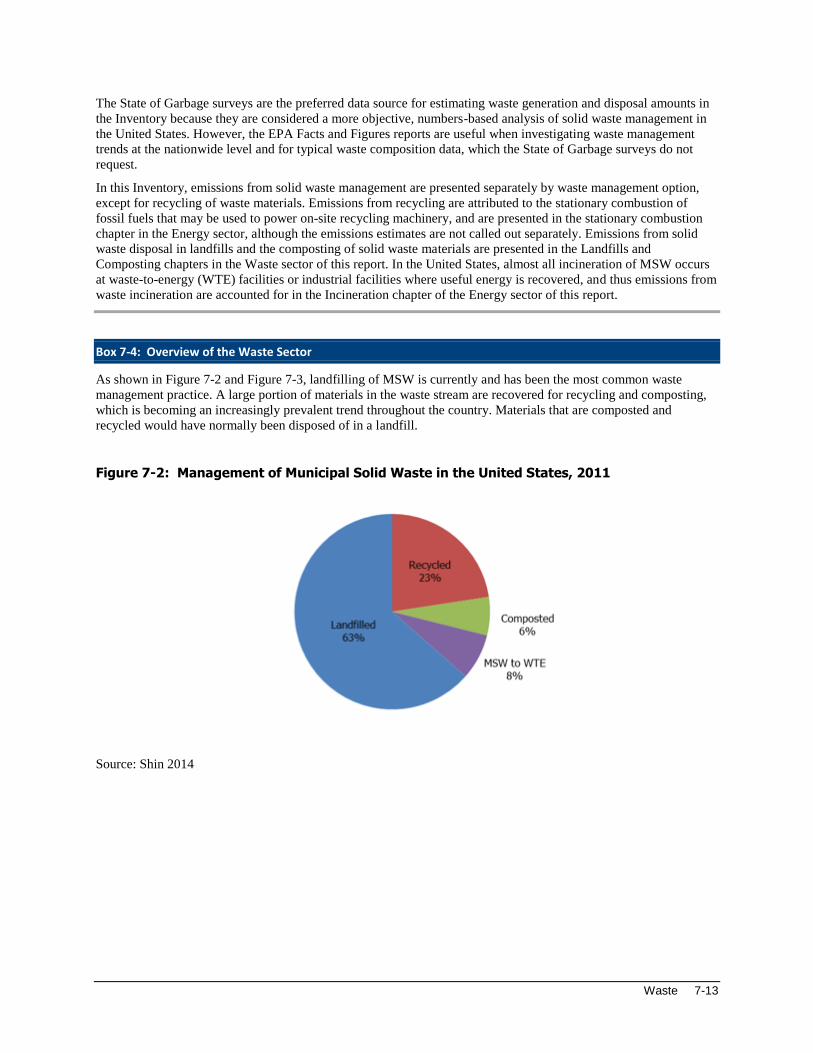
Waste 7-13
The State of Garbage surveys are the preferred data source for estimating waste generation and disposal amounts in
the Inventory because they are considered a more objective, numbers-based analysis of solid waste management in
the United States. However, the EPA Facts and Figures reports are useful when investigating waste management
trends at the nationwide level and for typical waste composition data, which the State of Garbage surveys do not
request.
In this Inventory, emissions from solid waste management are presented separately by waste management option,
except for recycling of waste materials. Emissions from recycling are attributed to the stationary combustion of
fossil fuels that may be used to power on-site recycling machinery, and are presented in the stationary combustion
chapter in the Energy sector, although the emissions estimates are not called out separately. Emissions from solid
waste disposal in landfills and the composting of solid waste materials are presented in the Landfills and
Composting chapters in the Waste sector of this report. In the United States, almost all incineration of MSW occurs
at waste-to-energy (WTE) facilities or industrial facilities where useful energy is recovered, and thus emissions from
waste incineration are accounted for in the Incineration chapter of the Energy sector of this report.
Box 7-4: Overview of the Waste Sector
As shown in Figure 7-2 and Figure 7-3, landfilling of MSW is currently and has been the most common waste
management practice. A large portion of materials in the waste stream are recovered for recycling and composting,
which is becoming an increasingly prevalent trend throughout the country. Materials that are composted and
recycled would have normally been disposed of in a landfill.
Figure 7-2: Management of Municipal Solid Waste in the United States, 2011
Source: Shin 2014

7-14 Inventory of U.S. Greenhouse Gas Emissions and Sinks: 1990–2013
Figure 7-3: MSW Management Trends from 1990 to 2012
Source: EPA 2014c
Table 7-6 presents a typical composition of waste disposed of at a typical MSW landfill in the United States over
time. It is important to note that the actual composition of waste entering each landfill will vary from that presented
in Table 7-6. Understanding how the waste composition changes over time, specifically for the degradable waste
types, is important for estimating greenhouse gas emissions. For certain degradable waste types (i.e., paper and
paperboard), the amounts discarded have decreased over time due to an increase in waste recovery, including
recycling and composting (see Table 7-6 and Figure 7-4). Landfill ban legislation affecting yard trimmings resulted
in an increase of composting from 1990 to 2008. Table 7-6 and Figure 7-4 do not reflect the impact of backyard
composting on yard trimming generation and recovery estimates. The recovery of food trimmings has been
consistently low. Increased recovery of degradable materials reduces the CH4 generation potential and CH4
emissions from landfills.

Waste 7-15
Table 7-6: Materials Discarded in the Municipal Waste Stream by Waste Type (Percent)
Waste Type 1990 2005
2009 2010 2011 2012
Paper and Paperboard 30.0% 24.5% 14.8% 16.2% 14.8% 14.8%
Glass 6.0% 5.7% 5.0% 5.1% 5.1% 5.1%
Metals 7.2% 7.7% 8.0% 8.8% 8.9% 9.0%
Plastics 9.6% 15.7% 15.8% 17.4% 17.8% 17.6%
Rubber and Leather 3.1% 3.5% 3.7% 3.7% 3.8% 3.8%
Textiles 2.9% 5.5% 6.3% 6.7% 6.8% 7.4%
Wood 6.9% 7.4% 7.7% 8.1% 8.2% 8.2%
Othera 1.4% 1.8% 1.9% 2.0% 2.0% 2.0%
Food Scrapsb 13.6% 17.9% 19.1% 21.0% 21.4% 21.1%
Yard Trimmingsc 17.6% 7.0% 7.6% 8.6% 8.8% 8.7%
Miscellaneous Inorganic
Wastes 1.7% 2.1% 2.2% 2.3% 2.4% 2.4%
a Includes electrolytes in batteries and fluff pulp, feces, and urine in disposable diapers. Details may
not add to totals due to rounding. Source: EPA 2014c. b Data for food scraps were estimated using sampling studies in various parts of the country in
combination with demographic data on population, grocery store sales, restaurant sales, number of
employees, and number of prisoners, students, and patients in institutions. Source: EPA 2014c. c Data for yard trimmings were estimated using sampling studies, population data, and published
sources documenting legislation affecting yard trimmings disposal in landfills. Source: EPA 2014c.
Figure 7-4: Percent of Recovered Degradable Materials from 1990 to 2012 (Percent)
Source: EPA 2014c
Box 7-5: Description of a Modern, Managed Landfill
Modern, managed landfills are well-engineered facilities that are located, designed, operated, and monitored to
ensure compliance with federal, state, and tribal regulations. Municipal solid waste (MSW) landfills must be
designed to protect the environment from contaminants which may be present in the solid waste stream.
Additionally, many new landfills collect and destroy landfill gas through flares or landfill gas-to-energy projects.
Requirements for affected MSW landfills may include:
Siting requirements to protect sensitive areas (e.g., airports, floodplains, wetlands, fault areas,
seismic impact zones, and unstable areas)

7-16 Inventory of U.S. Greenhouse Gas Emissions and Sinks: 1990–2013
Design requirements for new landfills to ensure that Maximum Contaminant Levels (MCLs) will
not be exceeded in the uppermost aquifer (e.g., composite liners and leachate collection systems)
Leachate collection and removal systems
Operating practices (e.g., daily and intermediate cover, receipt of regulated hazardous wastes, use
of landfill cover material, access options to prevent illegal dumping, use of a collection system to prevent
stormwater run-on/run-off, record-keeping)
Air monitoring requirements (explosive gases)
Groundwater monitoring requirements
Closure and post-closure care requirements (e.g., final cover construction), and
Corrective action provisions.
Specific federal regulations that affected MSW landfills must comply with include the 40 CFR Part 258 (Subtitle D
of RCRA), or equivalent state regulations and the New Source Performance Standards (NSPS) 40 CFR Part 60
Subpart WWW. Additionally, state and tribal requirements may exist.9
7.2 Wastewater Treatment (IPCC Source Category 5D)
Wastewater treatment processes can produce anthropogenic CH4 and N2O emissions. Wastewater from domestic10
and industrial sources is treated to remove soluble organic matter, suspended solids, pathogenic organisms, and
chemical contaminants. Treatment may either occur on site, most commonly through septic systems or package
plants, or off site at centralized treatment systems. Centralized wastewater treatment systems may include a variety
of processes, ranging from lagooning to advanced tertiary treatment technology for removing nutrients. In the
United States, approximately 20 percent of domestic wastewater is treated in septic systems or other on-site systems,
while the rest is collected and treated centrally (U.S. Census Bureau 2011).
Soluble organic matter is generally removed using biological processes in which microorganisms consume the
organic matter for maintenance and growth. The resulting biomass (sludge) is removed from the effluent prior to
discharge to the receiving stream. Microorganisms can biodegrade soluble organic material in wastewater under
aerobic or anaerobic conditions, where the latter condition produces CH4. During collection and treatment,
wastewater may be accidentally or deliberately managed under anaerobic conditions. In addition, the sludge may be
further biodegraded under aerobic or anaerobic conditions. The generation of N2O may also result from the
treatment of domestic wastewater during both nitrification and denitrification of the N present, usually in the form of
urea, ammonia, and proteins. These compounds are converted to nitrate (NO3) through the aerobic process of
nitrification. Denitrification occurs under anoxic conditions (without free oxygen), and involves the biological
conversion of nitrate into dinitrogen gas (N2). N2O can be an intermediate product of both processes, but has
typically been associated with denitrification. Recent research suggests that higher emissions of N2O may in fact
originate from nitrification (Ahn et al. 2010). Other more recent research suggests that N2O may also result from
other types of wastewater treatment operations (Chandran 2012).
The principal factor in determining the CH4 generation potential of wastewater is the amount of degradable organic
material in the wastewater. Common parameters used to measure the organic component of the wastewater are the
Biochemical Oxygen Demand (BOD) and Chemical Oxygen Demand (COD). Under the same conditions,
wastewater with higher COD (or BOD) concentrations will generally yield more CH4 than wastewater with lower
COD (or BOD) concentrations. BOD represents the amount of oxygen that would be required to completely
9 For more information regarding federal MSW landfill regulations, see
<http://www.epa.gov/osw/nonhaz/municipal/landfill/msw_regs.htm>. 10 Throughout the inventory, emissions from domestic wastewater also include any commercial and industrial wastewater
collected and co-treated with domestic wastewater.

Waste 7-17
consume the organic matter contained in the wastewater through aerobic decomposition processes, while COD
measures the total material available for chemical oxidation (both biodegradable and non-biodegradable). Because
BOD is an aerobic parameter, it is preferable to use COD to estimate CH4 production. The principal factor in
determining the N2O generation potential of wastewater is the amount of N in the wastewater. The variability of N
in the influent to the treatment system, as well as the operating conditions of the treatment system itself, also impact
the N2O generation potential.
In 2013, CH4 emissions from domestic wastewater treatment were 9.2 MMT CO2 Eq. (368 kt CH4). Emissions
remained fairly steady from 1990 through 1997, but have decreased since that time due to decreasing percentages of
wastewater being treated in anaerobic systems, including reduced use of on-site septic systems and central anaerobic
treatment systems (EPA 1992, 1996, 2000, and 2004, U.S. Census 2011). In 2013, CH4 emissions from industrial
wastewater treatment were estimated to be 5.8 MMT CO2 Eq. (233 kt CH4). Industrial emission sources have
generally increased across the time series through 1999 and then fluctuated up and down with production changes
associated with the treatment of wastewater from the pulp and paper manufacturing, meat and poultry processing,
fruit and vegetable processing, starch-based ethanol production, and petroleum refining industries. Table 7-7 and
Table 7-8 provide CH4 and N2O emission estimates from domestic and industrial wastewater treatment.
With respect to N2O, the United States identifies two distinct sources for N2O emissions from domestic wastewater:
emissions from centralized wastewater treatment processes, and emissions from effluent from centralized treatment
systems that has been discharged into aquatic environments. The 2013 emissions of N2O from centralized
wastewater treatment processes and from effluent were estimated to be 0.3 MMT CO2 Eq. (1 kt N2O) and 4.6 MMT
CO2 Eq. (15 kt N2O), respectively. Total N2O emissions from domestic wastewater were estimated to be 4.9 MMT
CO2 Eq. (17 kt N2O). N2O emissions from wastewater treatment processes gradually increased across the time
series as a result of increasing U.S. population and protein consumption.
Table 7-7: CH4 and N2O Emissions from Domestic and Industrial Wastewater Treatment
(MMT CO2 Eq.)
Activity 1990 2005 2009 2010 2011 2012 2013
CH4 15.7 15.9 15.6 15.5 15.3 15.2 15.0
Domestic 10.5 10.0 9.8 9.6 9.4 9.3 9.2
Industriala 5.1 5.8 5.8 5.9 5.9 5.8 5.8
N2O 3.4 4.3 4.6 4.7 4.8 4.9 4.9
Domestic 3.4 4.3 4.6 4.7 4.8 4.9 4.9
Total 19.1 20.2 20.2 20.2 20.1 20.1 19.9
Note: Emissions values are presented in CO2 equivalent mass units using IPCC AR4 GWP values.
a Industrial activity includes the pulp and paper manufacturing, meat and poultry processing, fruit and
vegetable processing, starch-based ethanol production, and petroleum refining industries.
Note: Totals may not sum due to independent rounding.
Table 7-8: CH4 and N2O Emissions from Domestic and Industrial Wastewater Treatment (kt)
Activity 1990 2005 2009 2010 2011 2012 2013
CH4 626 635 623 619 610 606 601
Domestic 421 401 392 384 375 373 368
Industriala 206 234 231 235 235 233 233
N2O 11 15 16 16 16 16 17
Domestic 11 15 16 16 16 16 17
Note: Emissions values are presented in CO2 equivalent mass units using IPCC AR4 GWP values.
a Industrial activity includes the pulp and paper manufacturing, meat and poultry processing, fruit and
vegetable processing, starch-based ethanol production, and petroleum refining industries.
Note: Totals may not sum due to independent rounding.

7-18 Inventory of U.S. Greenhouse Gas Emissions and Sinks: 1990–2013
Methodology
Domestic Wastewater CH4 Emission Estimates
Domestic wastewater CH4 emissions originate from both septic systems and from centralized treatment systems,
such as publicly owned treatment works (POTWs). Within these centralized systems, CH4 emissions can arise from
aerobic systems that are not well managed or that are designed to have periods of anaerobic activity (e.g.,
constructed wetlands), anaerobic systems (anaerobic lagoons and facultative lagoons), and from anaerobic digesters
when the captured biogas is not completely combusted. CH4 emissions from septic systems were estimated by
multiplying the United States population by the percent of wastewater treated in septic systems (about 20 percent)
and an emission factor (10.7 g CH4/capita/day), and then converting the result to kt/year. CH4emissions from
POTWs were estimated by multiplying the total BOD5 produced in the United States by the percent of wastewater
treated centrally (about 80 percent), the relative percentage of wastewater treated by aerobic and anaerobic systems,
the relative percentage of wastewater facilities with primary treatment, the percentage of BOD5 treated after primary
treatment (67.5 percent), the maximum CH4-producing capacity of domestic wastewater (0.6), and the relative
MCFs for well-managed aerobic (zero), not well managed aerobic (0.3), and anaerobic (0.8) systems with all aerobic
systems assumed to be well-managed. CH4emissions from anaerobic digesters were estimated by multiplying the
amount of biogas generated by wastewater sludge treated in anaerobic digesters by the proportion of CH4 in digester
biogas (0.65), the density of CH4 (662 g CH4/m3 CH4), and the destruction efficiency associated with burning the
biogas in an energy/thermal device (0.99). The methodological equations are:
Emissions from Septic Systems = A
= USPOP × (% onsite) × (EFSEPTIC) × 1/10^9 × Days
Emissions from Centrally Treated Aerobic Systems = B
= [(% collected) × (total BOD5 produced) × (% aerobic) × (% aerobic w/out primary) + (% collected) × (total BOD5
produced) × (% aerobic) × (% aerobic w/primary) × (1-% BOD removed in prim. treat.)] × (% operations not well
managed) × (Bo) × (MCF-aerobic_not_well_man)
Emissions from Centrally Treated Anaerobic Systems = C
= [(% collected) × (total BOD5 produced) × (% anaerobic) × (% anaerobic w/out primary) + (% collected) × (total
BOD5 produced) × (% anaerobic) × (% anaerobic w/primary) × (1-%BOD removed in prim. treat.)] × (Bo) × (MCF-
anaerobic)
Emissions from Anaerobic Digesters = D
= [(POTW_flow_AD) × (digester gas)/ (per capita flow)] × conversion to m3 × (FRAC_CH4) × (365.25) × (density
of CH4) × (1-DE) × 1/10^9
Total CH4 Emissions (kt) = A + B + C + D
where,
USPOP = U.S. population
% onsite = Flow to septic systems / total flow
% collected = Flow to POTWs / total flow
% aerobic = Flow to aerobic systems / total flow to POTWs
% anaerobic = Flow to anaerobic systems / total flow to POTWs
% aerobic w/out primary = Percent of aerobic systems that do not employ primary treatment
% aerobic w/primary = Percent of aerobic systems that employ primary treatment
% BOD removed in prim. treat. = 32.5%
% operations not well managed = Percent of aerobic systems that are not well managed and in which
some anaerobic degradation occurs
% anaerobic w/out primary = Percent of anaerobic systems that do not employ primary treatment
% anaerobic w/primary = Percent of anaerobic systems that employ primary treatment
EFSEPTIC = Methane emission factor (10.7 g CH4/capita/day) – septic systems
Days = days per year (365.25)

Waste 7-19
Total BOD5 produced = kg BOD/capita/day × U.S. population × 365.25 days/yr
Bo = Maximum CH4-producing capacity for domestic wastewater (0.60 kg
CH4/kg BOD)
1/10^6 = Conversion factor, kg to kt
MCF-aerobic_not_well_man. = CH4 correction factor for aerobic systems that are not well managed
(0.3)
MCF-anaerobic = CH4 correction factor for anaerobic systems (0.8)
DE = CH4 destruction efficiency from flaring or burning in engine (0.99 for
enclosed flares)
POTW_flow_AD = Wastewater influent flow to POTWs that have anaerobic digesters
(MGD)
digester gas = Cubic feet of digester gas produced per person per day (1.0
ft3/person/day)
per capita flow = Wastewater flow to POTW per person per day (100 gal/person/day)
conversion to m3 = Conversion factor, ft3 to m3 (0.0283)
FRAC_CH4 = Proportion CH4 in biogas (0.65)
density of CH4 = 662 (g CH4/m3 CH4)
1/10^9 = Conversion factor, g to kt
U.S. population data were taken from the U.S. Census Bureau International Database (U.S. Census 2014) and
include the populations of the United States, American Samoa, Guam, Northern Mariana Islands, Puerto Rico, and
the Virgin Islands. Table 7-9 presents U.S. population and total BOD5 produced for 1990 through 2013, while Table
7-10 presents domestic wastewater CH4 emissions for both septic and centralized systems in 2013. The proportions
of domestic wastewater treated onsite versus at centralized treatment plants were based on data from the 1989, 1991,
1993, 1995, 1997, 1999, 2001, 2003, 2005, 2007, 2009, and 2011 American Housing Surveys conducted by the U.S.
Census Bureau (U.S. Census 2011), with data for intervening years obtained by linear interpolation and data for
2013 forecasted using 1990-2012 data. The percent of wastewater flow to aerobic and anaerobic systems, the
percent of aerobic and anaerobic systems that do and do not employ primary treatment, and the wastewater flow to
POTWs that have anaerobic digesters were obtained from the 1992, 1996, 2000, and 2004 Clean Watershed Needs
Survey (EPA 1992, 1996, 2000, and 2004). Data for intervening years were obtained by linear interpolation and the
years 2004 through 2013 were forecasted from the rest of the time series. The BOD5 production rate (0.09
kg/capita/day) and the percent BOD5 removed by primary treatment for domestic wastewater were obtained from
Metcalf and Eddy (2003). The maximum CH4-producing capacity (0.6 kg CH4/kg BOD5) and both MCFs used for
centralized treatment systems were taken from IPCC (2006), while the CH4 emission factor (10.7 g CH4/capita/day)
used for septic systems were taken from Leverenz et al. (2010). The CH4 destruction efficiency for methane
recovered from sludge digestion operations, 99 percent, was selected based on the range of efficiencies (98 to 100
percent) recommended for flares in AP-42 Compilation of Air Pollutant Emission Factors, Chapter 2.4 (EPA 1998),
efficiencies used to establish New Source Performance Standards (NSPS) for landfills, along with data from CAR
(2011), Sullivan (2007), Sullivan (2010), and UNFCCC (2012). The cubic feet of digester gas produced per person
per day (1.0 ft3/person/day) and the proportion of CH4 in biogas (0.65) come from Metcalf and Eddy (2003). The
wastewater flow to a POTW (100 gal/person/day) was taken from the Great Lakes-Upper Mississippi River Board
of State and Provincial Public Health and Environmental Managers, "Recommended Standards for Wastewater
Facilities (Ten-State Standards)” (2004).
Table 7-9: U.S. Population (Millions) and Domestic Wastewater BOD5 Produced (kt)
Year Population BOD5
1990 253 8,333
2005 300 9,853
2009 311 10,220
2010 313 10,303
2011 316 10,377
2012 318 10,452
2013 320 10,534

7-20 Inventory of U.S. Greenhouse Gas Emissions and Sinks: 1990–2013
Sources: U.S. Census Bureau (2014);
Metcalf & Eddy (2003).
Table 7-10: Domestic Wastewater CH4 Emissions from Septic and Centralized Systems (2013)
CH4 Emissions (MMT CO2 Eq.) % of Domestic Wastewater CH4
Septic Systems 6.0 65.5%
Centralized Systems (including anaerobic
sludge digestion) 3.2 34.5%
Total 9.2 100%
Note: Emission values are presented in CO2 equivalent mass units using IPCC AR4 GWP values.
Note: Totals may not sum due to independent rounding.
Industrial Wastewater CH4 Emission Estimates
Methane emission estimates from industrial wastewater were developed according to the methodology described in
IPCC (2006). Industry categories that are likely to produce significant CH4 emissions from wastewater treatment
were identified and included in the Inventory. The main criteria used to identify these industries are whether they
generate high volumes of wastewater, whether there is a high organic wastewater load, and whether the wastewater
is treated using methods that result in CH4 emissions. The top five industries that meet these criteria are pulp and
paper manufacturing; meat and poultry processing; vegetables, fruits, and juices processing; starch-based ethanol
production; and petroleum refining. Wastewater treatment emissions for these sectors for 2013 are displayed in
Table 7-11 below. Table 7-12 contains production data for these industries.
Table 7-11: Industrial Wastewater CH4 Emissions by Sector (2013)
CH4 Emissions (MMT CO2 Eq.) % of Industrial Wastewater CH4
Meat & Poultry 4.4 75%
Pulp & Paper 1.1 18%
Fruit & Vegetables 0.1 2%
Petroleum Refineries 0.1 2%
Ethanol Refineries 0.1 2%
Total 5.8 100%
Note: Emissions values are presented in CO2 equivalent mass units using IPCC AR4 GWP values.
Note: Totals may not sum due to independent rounding.
Table 7-12: U.S. Pulp and Paper, Meat, Poultry, Vegetables, Fruits and Juices, Ethanol, and Petroleum Refining Production (MMT)
Year
Pulp and
Papera
Meat
(Live Weight
Killed)
Poultry
(Live Weight
Killed)
Vegetables,
Fruits and
Juices Ethanol
Petroleum
Refining
1990 128.9 27.3 14.6 38.7 2.5 702.4
2005 138.5 31.4 25.1 42.9 11.7 818.6
2009 120.4 33.8 25.2 46.5 32.7 822.4
2010 128.6 33.7 25.9 43.2 39.7 848.6
2011 127.5 33.8 26.2 44.3 41.6 858.8
2012 127.0 33.8 26.1 45.3 39.5 856.1
2013 131.5 33.6 26.5 43.9 39.8 875.9
aPulp and paper production is the sum of woodpulp production plus paper and paperboard production.
Sources: Lockwood-Post (2002); FAO (2014); USDA (2014a); RFA (2014); EIA (2014).

Waste 7-21
CH4 emissions from these categories were estimated by multiplying the annual product output by the average
outflow, the organics loading (in COD) in the outflow, the maximum CH4 producing potential of industrial
wastewater (Bo), and the percentage of organic loading assumed to degrade anaerobically in a given treatment
system (MCF). Ratios of BOD:COD in various industrial wastewaters were obtained from EPA (1997a) and used to
estimate COD loadings. The Bo value used for all industries is the IPCC default value of 0.25 kg CH4/kg COD
(IPCC 2006).
For each industry, the percent of plants in the industry that treat wastewater on site, the percent of plants that have a
primary treatment step prior to biological treatment, and the percent of plants that treat wastewater anaerobically
were defined. The percent of wastewater treated anaerobically onsite (TA) was estimated for both primary treatment
(%TAp) and secondary treatment (%TAs). For plants that have primary treatment in place, an estimate of COD that
is removed prior to wastewater treatment in the anaerobic treatment units was incorporated. The values used in the
%TA calculations are presented in Table 7-13 below.
The methodological equations are:
CH4 (industrial wastewater) = [P W COD %TAp Bo MCF] + [P W COD %TAs Bo MCF]
%TAp = [%Plantso %WWa,p %CODp]
%TAs = [%Plantsa %WWa,s %CODs] + [%Plantst %WWa,t %CODs]
where,
CH4 (industrial wastewater) = Total CH4 emissions from industrial wastewater (kg/year)
P = Industry output (metric tons/year)
W = Wastewater generated (m3/metric ton of product)
COD = Organics loading in wastewater (kg/m3)
%TAp = Percent of wastewater treated anaerobically on site in primary treatment
%TAs = Percent of wastewater treated anaerobically on site in secondary treatment
%Plantso = Percent of plants with onsite treatment
%WWa,p = Percent of wastewater treated anaerobically in primary treatment
%CODp = Percent of COD entering primary treatment
%Plantsa = Percent of plants with anaerobic secondary treatment
%Plantst = Percent of plants with other secondary treatment
%WWa,s = Percent of wastewater treated anaerobically in anaerobic secondary treatment
%WWa,t = Percent of wastewater treated anaerobically in other secondary treatment
%CODs = Percent of COD entering secondary treatment
Bo = Maximum CH4 producing potential of industrial wastewater (default value of
0.25 kg CH4/kg COD)
MCF = CH4 correction factor, indicating the extent to which the organic content
(measured as COD) degrades anaerobically
Alternate methodological equations for calculating %TA were used for secondary treatment in the pulp and paper
industry to account for aerobic systems with anaerobic portions. These equations are:
%TAa = [%Plantsa × %WWas × %CODs]+[%Plantst × %WWat × CODs]
%TAat = [%Plantsat × %WWas × %CODs]
where,
%TAa = Percent of wastewater treated anaerobically on site in secondary treatment
%TAat = Percent of wastewater treated in aerobic systems with anaerobic portions on
site in secondary treatment
%Plantsa = Percent of plants with anaerobic secondary treatment
%Plantsa,t = Percent of plants with partially anaerobic secondary treatment
%WWa,s = Percent of wastewater treated anaerobically in anaerobic secondary treatment
%WWa,t = Percent of wastewater treated anaerobically in other secondary treatment

7-22 Inventory of U.S. Greenhouse Gas Emissions and Sinks: 1990–2013
%CODs = Percent of COD entering secondary treatment
As described below, the values presented in Table 7-13 were used in the emission calculations and are described in
detail in ERG (2008), ERG (2013a), and ERG (2013b).
Table 7-13: Variables Used to Calculate Percent Wastewater Treated Anaerobically by
Industry (percent)
Variable
Industry
Pulp
and
Paper
Meat
Processing
Poultry
Processing
Fruit/
Vegetable
Processing
Ethanol
Production
– Wet Mill
Ethanol
Production
– Dry Mill
Petroleum
Refining
%TAp 0 0 0 0 0 0 0
%TAs 0 33 25 4.2 33.3 75 23.6
%TAa 2.2 0 0 0 0 0 0
%TAa,t 11.8 0 0 0 0 0 0
%Plantso 0 100 100 11 100 100 100
%Plantsa 5 33 25 5.5 33.3 75 23.6
%Plantsa,t 28 0 0 0 0 0 0
%Plantst 35 67 75 5.5 66.7 25 0
%WWa,p 0 0 0 0 0 0 0
%WWa,s 100 100 100 100 100 100 100
%WWa,t 0 0 0 0 0 0 0
%CODp 100 100 100 100 100 100 100
%CODs 42 100 100 77 100 100 100
Sources: ERG (2008); ERG (2013a); and ERG (2013b).
Pulp and Paper. Wastewater treatment for the pulp and paper industry typically includes neutralization, screening,
sedimentation, and flotation/hydrocycloning to remove solids (World Bank 1999, Nemerow and Dasgupta 1991).
Secondary treatment (storage, settling, and biological treatment) mainly consists of lagooning. In determining the
percent that degrades anaerobically, both primary and secondary treatment were considered. In the United States,
primary treatment is focused on solids removal, equalization, neutralization, and color reduction (EPA 1993). The
vast majority of pulp and paper mills with on-site treatment systems use mechanical clarifiers to remove suspended
solids from the wastewater. About 10 percent of pulp and paper mills with treatment systems use settling ponds for
primary treatment and these are more likely to be located at mills that do not perform secondary treatment (EPA
1993). However, because the vast majority of primary treatment operations at U.S. pulp and paper mills use
mechanical clarifiers, and less than 10 percent of pulp and paper wastewater is managed in primary settling ponds
that are not expected to have anaerobic conditions, negligible emissions are assumed to occur during primary
treatment.
Approximately 42 percent of the BOD passes on to secondary treatment, which consists of activated sludge, aerated
stabilization basins, or non-aerated stabilization basins. Based on EPA’s OAQPS Pulp and Paper Sector Survey, 5.3
percent of pulp and paper mills reported using anaerobic secondary treatment for wastewater and/or pulp
condensates (ERG 2013a). Twenty-eight percent (28 percent) of mills also reported the use of quiescent settling
ponds. Using engineering judgment, these systems were determined to be aerobic with possible anaerobic portions.
For the truly anaerobic systems, an MCF of 0.8 is used, as these are typically deep stabilization basins. For the
partially anaerobic systems, an MCF of 0.2 is used, which is the IPCC suggested MCF for shallow lagoons.
A time series of CH4 emissions for 1990 through 2001 was developed based on production figures reported in the
Lockwood-Post Directory (Lockwood-Post 2002). Data from the Food and Agricultural Organization of the United
Nations (FAO) database FAOSTAT were used for 2002 through 2013 (FAO 2014). The overall wastewater outflow
varies based on a time series outlined in ERG (2013a) to reflect historical and current industry wastewater flow, and
the average BOD concentrations in raw wastewater was estimated to be 0.4 gram BOD/liter (EPA 1997b, EPA
1993, World Bank 1999). The COD:BOD ratio used to convert the organic loading to COD for pulp and paper mills
was 2 (EPA 1997a).

Waste 7-23
Meat and Poultry Processing. The meat and poultry processing industry makes extensive use of anaerobic lagoons
in sequence with screening, fat traps, and dissolved air flotation when treating wastewater on site. About 33 percent
of meat processing operations (EPA 2002) and 25 percent of poultry processing operations (U.S. Poultry 2006)
perform on-site treatment in anaerobic lagoons. The IPCC default Bo of 0.25 kg CH4/kg COD and default MCF of
0.8 for anaerobic lagoons were used to estimate the CH4 produced from these on-site treatment systems. Production
data, in carcass weight and live weight killed for the meat and poultry industry, were obtained from the USDA
Agricultural Statistics Database and the Agricultural Statistics Annual Reports (USDA 2014a). Data collected by
EPA’s Office of Water provided estimates for wastewater flows into anaerobic lagoons: 5.3 and 12.5 m3/metric ton
for meat and poultry production (live weight killed), respectively (EPA 2002). The loadings are 2.8 and 1.5 g
BOD/liter for meat and poultry, respectively. The COD:BOD ratio used to convert the organic loading to COD for
both meat and poultry facilities was 3 (EPA 1997a).
Vegetables, Fruits, and Juices Processing. Treatment of wastewater from fruits, vegetables, and juices processing
includes screening, coagulation/settling, and biological treatment (lagooning). The flows are frequently seasonal,
and robust treatment systems are preferred for on-site treatment. Effluent is suitable for discharge to the sewer.
This industry is likely to use lagoons intended for aerobic operation, but the large seasonal loadings may develop
limited anaerobic zones. In addition, some anaerobic lagoons may also be used (Nemerow and Dasgupta 1991).
Consequently, 4.2 percent of these wastewater organics are assumed to degrade anaerobically. The IPCC default Bo
of 0.25 kg CH4/kg COD and default MCF of 0.8 for anaerobic treatment were used to estimate the CH4 produced
from these on-site treatment systems. The USDA National Agricultural Statistics Service (USDA 2014a) provided
production data for potatoes, other vegetables, citrus fruit, non-citrus fruit, and grapes processed for wine. Outflow
and BOD data, presented in Table 7-14, were obtained from EPA (1974) for potato, citrus fruit, and apple
processing, and from EPA (1975) for all other sectors. The COD:BOD ratio used to convert the organic loading to
COD for all fruit, vegetable, and juice facilities was 1.5 (EPA 1997a).
Table 7-14: Wastewater Flow (m3/ton) and BOD Production (g/L) for U.S. Vegetables, Fruits,
and Juices Production
Commodity Wastewater Outflow (m3/ton) BOD (g/L)
Vegetables Potatoes 10.27 1.765 Other Vegetables 8.67 0.791
Fruit Apples 3.66 1.371 Citrus 10.11 0.317 Non-citrus 12.42 1.204 Grapes (for wine) 2.78 1.831
Sources: EPA 1974, EPA 1975.
Ethanol Production. Ethanol, or ethyl alcohol, is produced primarily for use as a fuel component, but is also used in
industrial applications and in the manufacture of beverage alcohol. Ethanol can be produced from the fermentation
of sugar-based feedstocks (e.g., molasses and beets), starch- or grain-based feedstocks (e.g., corn, sorghum, and
beverage waste), and cellulosic biomass feedstocks (e.g., agricultural wastes, wood, and bagasse). Ethanol can also
be produced synthetically from ethylene or hydrogen and carbon monoxide. However, synthetic ethanol comprises
only about 2 percent of ethanol production, and although the Department of Energy predicts cellulosic ethanol to
greatly increase in the coming years, currently it is only in an experimental stage in the United States. Currently,
ethanol is mostly made from sugar and starch crops, but with advances in technology, cellulosic biomass is
increasingly used as ethanol feedstock (DOE 2013).
Ethanol is produced from corn (or other starch-based feedstocks) primarily by two methods: wet milling and dry
milling. Historically, the majority of ethanol was produced by the wet milling process, but now the majority is
produced by the dry milling process. The dry milling process is cheaper to implement, and has become more
efficient in recent years (Rendleman and Shapouri 2007). The wastewater generated at ethanol production facilities
is handled in a variety of ways. Dry milling facilities often combine the resulting evaporator condensate with other
process wastewaters, such as equipment wash water, scrubber water, and boiler blowdown and anaerobically treat
this wastewater using various types of digesters. Wet milling facilities often treat their steepwater condensate in
anaerobic systems followed by aerobic polishing systems. Wet milling facilities may treat the stillage (or processed

7-24 Inventory of U.S. Greenhouse Gas Emissions and Sinks: 1990–2013
stillage) from the ethanol fermentation/distillation process separately or together with steepwater and/or wash water.
CH4 generated in anaerobic digesters is commonly collected and either flared or used as fuel in the ethanol
production process (ERG 2006).
Available information was compiled from the industry on wastewater generation rates, which ranged from 1.25
gallons per gallon ethanol produced (for dry milling) to 10 gallons per gallon ethanol produced (for wet milling)
(Ruocco 2006a,b; Merrick 1998; Donovan 1996; and NRBP 2001). COD concentrations were also found to be
about 3 g/L (Ruocco 2006a; Merrick 1998; White and Johnson 2003). The amount of wastewater treated
anaerobically was estimated, along with how much of the CH4 is recovered through the use of biomethanators.
Biomethanators are anaerobic reactors that use microorganisms under anaerobic conditions to reduce COD and
organic acids and recover biogas from wastewater (ERG 2006). Methane emissions were then estimated as follows:
Methane = [Production × Flow × COD × 3.785 × ([%Plantso × %WWa,p × %CODp] + [%Plantsa × %WWa,s × %CODs] +
[%Plantst × %WWa,t × %CODs]) × Bo × MCF × % Not Recovered] + [Production × Flow × 3.785 × COD × ([%Plantso ×
%WWa,p × %CODp] + [%Plantsa × %WWa,s × %CODs] + [%Plantst × %WWa,t × %CODs]) × Bo × MCF × (% Recovered) × (1-
DE)] × 1/10^9
where,
Production = gallons ethanol produced (wet milling or dry milling)
Flow = gallons wastewater generated per gallon ethanol produced (1.25 dry milling, 10 wet milling)
COD = COD concentration in influent (3 g/l)
3.785 = conversion, gallons to liters
%Plantso = percent of plants with onsite treatment (100%)
%WWa,p = percent of wastewater treated anaerobically in primary treatment (0%)
%CODp = percent of COD entering primary treatment (100%)
%Plantsa = percent of plants with anaerobic secondary treatment (33.3% wet, 75% dry)
%Plantst = percent of plants with other secondary treatment (66.7% wet, 25% dry)
%WWa,s = percent of wastewater treated anaerobically in anaerobic secondary treatment (100%)
%WWa,t = percent of wastewater treated anaerobically in other secondary treatment (0%)
%CODs = percent of COD entering secondary treatment (100%)
Bo = maximum methane producing capacity (0.25 g CH4/g COD)
MCF = methane conversion factor (0.8 for anaerobic systems)
% Recovered = percent of wastewater treated in system with emission recovery
% Not Recovered = 1 - percent of wastewater treated in system with emission recovery
DE = destruction efficiency of recovery system (99%)
1/10^9 = conversion factor, g to kt
A time series of CH4 emissions for 1990 through 2013 was developed based on production data from the Renewable
Fuels Association (RFA 2014).
Petroleum Refining. Petroleum refining wastewater treatment operations have the potential to produce CH4
emissions from anaerobic wastewater treatment. EPA’s Office of Air and Radiation performed an Information
Collection Request (ICR) for petroleum refineries in 2011.11 Of the responding facilities, 23.6 percent reported
using non-aerated surface impoundments or other biological treatment units, both of which have the potential to lead
to anaerobic conditions (ERG 2013b). In addition, the wastewater generation rate was determined to be 26.4 gallons
per barrel of finished product (ERG 2013b). An average COD value in the wastewater was estimated at 0.45 kg/m3
(Benyahia et al. 2006).
The equation used to calculate CH4 generation at petroleum refining wastewater treatment systems is presented
below:
Methane = Flow × COD × TA × Bo × MCF
where,
Flow = Annual flow treated through anaerobic treatment system (m3/year)
COD = COD loading in wastewater entering anaerobic treatment system (kg/m3)
TA = Percent of wastewater treated anaerobically on site
11 Available online at <https://refineryicr.rti.org/>.

Waste 7-25
Bo = maximum methane producing potential of industrial wastewater (default value of 0.25
kg CH4 /kg COD)
MCF = methane conversion factor (0.3)
A time series of CH4 emissions for 1990 through 2013 was developed based on production data from the Energy
Information Association (EIA 2014).
Domestic Wastewater N2O Emission Estimates
N2O emissions from domestic wastewater (wastewater treatment) were estimated using the IPCC (2006)
methodology, including calculations that take into account N removal with sewage sludge, non-consumption and
industrial/commercial wastewater N, and emissions from advanced centralized wastewater treatment plants:
In the United States, a certain amount of N is removed with sewage sludge, which is applied to land, incinerated,
or landfilled (NSLUDGE). The N disposal into aquatic environments is reduced to account for the sewage sludge
application.
The IPCC methodology uses annual, per capita protein consumption (kg protein/person-year). For this
inventory, the amount of protein available to be consumed is estimated based on per capita annual food
availability data and its protein content, and then adjusts that data using a factor to account for the fraction of
protein actually consumed.
Small amounts of gaseous nitrogen oxides are formed as byproducts in the conversion of nitrate to N gas in
anoxic biological treatment systems. Approximately 7 g N2O is generated per capita per year if wastewater
treatment includes intentional nitrification and denitrification (Scheehle and Doorn 2001). Analysis of the 2004
CWNS shows that plants with denitrification as one of their unit operations serve a population of 2.4 million
people. Based on an emission factor of 7 g per capita per year, approximately 21.2 metric tons of additional N2O
may have been emitted via denitrification in 2004. Similar analyses were completed for each year in the
Inventory using data from CWNS on the amount of wastewater in centralized systems treated in denitrification
units. Plants without intentional nitrification/denitrification are assumed to generate 3.2 g N2O per capita per
year.
N2O emissions from domestic wastewater were estimated using the following methodology:
N2OTOTAL = N2OPLANT + N2OEFFLUENT
N2OPLANT = N2ONIT/DENIT + N2OWOUT NIT/DENIT
N2ONIT/DENIT = [(USPOPND) × EF2 × FIND-COM] × 1/10^9
N2OWOUT NIT/DENIT = {[(USPOP × WWTP) - USPOPND]× FIND-COM × EF1} × 1/10^9
N2OEFFLUENT = {[(((USPOP × WWTP) – (0.9 × USPOPND)) × Protein × FNPR × FNON-CON × FIND-COM) - NSLUDGE] × EF3 ×
44/28} × 1/10^6
where,
N2OTOTAL = Annual emissions of N2O (kt)
N2OPLANT = N2O emissions from centralized wastewater treatment plants (kt)
N2ONIT/DENIT = N2O emissions from centralized wastewater treatment plants with
nitrification/denitrification (kt)
N2OWOUT NIT/DENIT = N2O emissions from centralized wastewater treatment plants without
nitrification/denitrification (kt)
N2OEFFLUENT = N2O emissions from wastewater effluent discharged to aquatic environments (kt)
USPOP = U.S. population
USPOPND = U.S. population that is served by biological denitrification (from CWNS)
WWTP = Fraction of population using WWTP (as opposed to septic systems)
EF1 = Emission factor (3.2 g N2O/person-year) – plant with no intentional denitrification
EF2 = Emission factor (7 g N2O/person-year) – plant with intentional denitrification
Protein = Annual per capita protein consumption (kg/person/year)
FNPR = Fraction of N in protein, default = 0.16 (kg N/kg protein)

7-26 Inventory of U.S. Greenhouse Gas Emissions and Sinks: 1990–2013
FNON-CON = Factor for non-consumed protein added to wastewater (1.4)
FIND-COM = Factor for industrial and commercial co-discharged protein into the sewer system
(1.25)
NSLUDGE = N removed with sludge, kg N/yr
EF3 = Emission factor (0.005 kg N2O -N/kg sewage-N produced) – from effluent
0.9 = Amount of nitrogen removed by denitrification systems
44/28 = Molecular weight ratio of N2O to N2
U.S. population data were taken from the U.S. Census Bureau International Database (U.S. Census 2014) and
include the populations of the United States, American Samoa, Guam, Northern Mariana Islands, Puerto Rico, and
the Virgin Islands. The fraction of the U.S. population using wastewater treatment plants is based on data from the
1989, 1991, 1993, 1995, 1997, 1999, 2001, 2003, 2005, 2007, 2009, and 2011 American Housing Survey (U.S.
Census 2011). Data for intervening years were obtained by linear interpolation and data from 2012 and 2013 were
forecasted using 1990-2011 data. The emission factor (EF1) used to estimate emissions from wastewater treatment
for plants without intentional denitrification was taken from IPCC (2006), while the emission factor (EF2) used to
estimate emissions from wastewater treatment for plants with intentional denitrification was taken from Scheehle
and Doorn (2001). Data on annual per capita protein intake were provided by the U.S. Department of Agriculture
Economic Research Service (USDA 2014b). Protein consumption data for 2010 through 2013 were extrapolated
from data for 1990 through 2006. An emission factor to estimate emissions from effluent (EF3) has not been
specifically estimated for the United States, thus the default IPCC value (0.005 kg N2O-N/kg sewage-N produced)
was applied (IPCC 2006). The fraction of N in protein (0.16 kg N/kg protein) was also obtained from IPCC (2006).
The factor for non-consumed protein and the factor for industrial and commercial co-discharged protein were
obtained from IPCC (2006). Sludge generation was obtained from EPA (1999) for 1988, 1996, and 1998 and from
Beecher et al. (2007) for 2004. Intervening years were interpolated, and estimates for 2005 through 2012 were
forecasted from the rest of the time series. The amount of nitrogen removed by denitrification systems was taken
from EPA (2008). An estimate for the N removed as sludge (NSLUDGE) was obtained by determining the amount of
sludge disposed by incineration, by land application (agriculture or other), through surface disposal, in landfills, or
through ocean dumping (US EPA 1993b, Beecher et al. 2007, McFarland 2001, US EPA 1999). In 2013, 286 kt N
was removed with sludge. Table 7-15 presents the data for U.S. population, population served by biological
denitrification, population served by wastewater treatment plants, available protein, protein consumed, and nitrogen
removed with sludge.
Table 7-15: U.S. Population (Millions), Population Served by Biological Denitrification (Millions), Fraction of Population Served by Wastewater Treatment (percent), Available
Protein (kg/person-year), Protein Consumed (kg/person-year), and Nitrogen Removed with
Sludge (kt-N/year)
Year Population PopulationND WWTP Population Available Protein Protein Consumed N Removed
1990 253 2.0 75.6 38.4 29.5 214.1
2005 300 2.7 78.8 39.8 30.7 261.1
2009 311 2.9 79.3 40.9 31.5 273.4
2010 313 3.0 80.0 41.0 31.6 276.4
2011 316 3.0 80.6 41.1 31.7 279.5
2012 318 3.0 80.4 41.2 31.8 282.6
2013 320 3.1 80.7 41.3 31.9 285.6
Sources: Beecher et al. 2007, McFarland 2001, U.S. Census 2011, U.S. Census 2014, USDA 2014b, US EPA 1992, US EPA
1993b, US EPA 1996, US EPA 1999, US EPA 2000, US EPA 2004.
Uncertainty and Time-Series Consistency The overall uncertainty associated with both the 2013 CH4 and N2O emission estimates from wastewater treatment
and discharge was calculated using the 2006 IPCC Guidelines Approach 2 methodology (2006). Uncertainty
associated with the parameters used to estimate CH4 emissions include that of numerous input variables used to
model emissions from domestic wastewater, and wastewater from pulp and paper manufacture, meat and poultry
processing, fruits and vegetable processing, ethanol production, and petroleum refining. Uncertainty associated with

Waste 7-27
the parameters used to estimate N2O emissions include that of sewage sludge disposal, total U.S. population,
average protein consumed per person, fraction of N in protein, non-consumption nitrogen factor, emission factors
per capita and per mass of sewage-N, and for the percentage of total population using centralized wastewater
treatment plants.
The results of this Approach 2 quantitative uncertainty analysis are summarized in Table 7-16. Methane emissions
from wastewater treatment were estimated to be between 9.2 and 15.3 MMT CO2 Eq. at the 95 percent confidence
level (or in 19 out of 20 Monte Carlo Stochastic Simulations). This indicates a range of approximately 39 percent
below to 2 percent above the 2013 emissions estimate of 15.0 MMT CO2 Eq. N2O emissions from wastewater
treatment were estimated to be between 1.2 and 10.2 MMT CO2 Eq., which indicates a range of approximately 76
percent below to 107 percent above the 2013 emissions estimate of 4.9 MMT CO2 Eq.
Table 7-16: Approach 2 Quantitative Uncertainty Estimates for CH4 Emissions from
Wastewater Treatment (MMT CO2 Eq. and Percent)
Source Gas
2013 Emission Estimate Uncertainty Range Relative to Emission Estimatea
(MMT CO2 Eq.) (MMT CO2 Eq.) (%)
Lower
Bound
Upper
Bound
Lower
Bound
Upper
Bound
Wastewater Treatment CH4 15.0 9.2 15.3 -39% +2%
Domestic CH4 9.2 5.7 9.9 -38% +7%
Industrial CH4 5.8 2.4 6.9 -59% +18%
Wastewater Treatment N2O 4.9 1.2 10.2 -76% +107%
a Range of emission estimates predicted by Monte Carlo Stochastic Simulation for a 95 percent
confidence interval.
Methodological recalculations were applied to the entire time-series to ensure time-series consistency from 1990
through 2013. Details on the emission trends through time are described in more detail in the Methodology section,
above.
QA/QC and Verification A QA/QC analysis was performed on activity data, documentation, and emission calculations. This effort included a
Tier 1 analysis, including the following checks:
Checked for transcription errors in data input;
Ensured references were specified for all activity data used in the calculations;
Checked a sample of each emission calculation used for the source category;
Checked that parameter and emission units were correctly recorded and that appropriate conversion factors
were used;
Checked for temporal consistency in time series input data for each portion of the source category;
Confirmed that estimates were calculated and reported for all portions of the source category and for all years;
Investigated data gaps that affected emissions estimates trends; and
Compared estimates to previous estimates to identify significant changes.
All transcription errors identified were corrected. The QA/QC analysis did not reveal any systemic inaccuracies or
incorrect input values.
Recalculations Discussion Production data were updated to reflect revised USDA NASS datasets. In addition, the most recent USDA ERS data
were used to update percent protein values from 1990 through 2010. The updated ERS data also resulted in small
changes in forecasted values from 2011. The factor for sewage sludge production change per year was updated to
include all available data. This change resulted in updated 1990 through 1995 values for total N in sludge along with
a change in forecasted values from 2005 through 2012.

7-28 Inventory of U.S. Greenhouse Gas Emissions and Sinks: 1990–2013
Workbooks were also updated to show emissions in kilotons and MMT CO2 Eq. In addition, global warming
potentials for N2O and CH4 were updated with the AR4 100-year values (IPCC 2007).
For the current Inventory, emission estimates have been revised to reflect the GWPs provided in the IPCC Fourth
Assessment Report (AR4) (IPCC 2007). AR4 GWP values differ slightly from those presented in the IPCC Second
Assessment Report (SAR) (IPCC 1996) (used in the previous inventories) which results in time-series recalculations
for most inventory sources. Under the most recent reporting guidelines (UNFCCC 2014), countries are required to
report using the AR4 GWPs, which reflect an updated understanding of the atmospheric properties of each
greenhouse gas. The GWPs of CH4 and most fluorinated greenhouse gases have increased, leading to an overall
increase in CO2-equivalent emissions from CH4. The GWPs of N2O and SF6 have decreased, leading to a decrease in
CO2-equivalent emissions for N2O. The AR4 GWPs have been applied across the entire time series for consistency.
For more information please see the Recalculations and Improvements Chapter.
Planned Improvements The methodology to estimate CH4 emissions from domestic wastewater treatment currently utilizes estimates for the
percentage of centrally treated wastewater that is treated by aerobic systems and anaerobic systems. These data
come from the 1992, 1996, 2000, and 2004 CWNS. The question of whether activity data for wastewater treatment
systems are sufficient across the time series to further differentiate aerobic systems with the potential to generate
small amounts of CH4 (aerobic lagoons) versus other types of aerobic systems, and to differentiate between
anaerobic systems to allow for the use of different MCFs for different types of anaerobic treatment systems,
continues to be explored. The CWNS data for 2008 were evaluated for incorporation into the Inventory, but due to
significant changes in format, this dataset is not sufficiently detailed for inventory calculations. However, additional
information and other data continue to be evaluated to update future years of the Inventory, including anaerobic
digester data compiled by the North East Biosolids and Residuals Association (NEBRA) in collaboration with
several other entities. While NEBRA is no longer involved in the project, the Water Environment Federation (WEF)
now hosts and manages the dataset which has been relocated to www.wef.org/biosolids. WEF will complete the
second phase of their data collection and by late fall. They are currently collecting additional data on a Region by
Region basis which should add to the quality of the database by decreasing uncertainty and data gaps (ERG 2014a).
EPA will continue to monitor the status of these data as a potential source of digester, sludge, and biogas data from
POTWs.
Data collected under the EPA’s Greenhouse Gas Reporting Program Subpart II, Industrial Wastewater Treatment
(GHGRP) is being investigated for use in improving the emission estimates for the industrial wastewater category.
Ensuring time series consistency has been the focus, as the reporting data from EPA’s GHGRP are not available for
all inventory years. Whether EPA’s GHGRP reporters sufficiently represent U.S. emissions is being investigated to
determine if moving to a facility-level implementation of GHGRP data is warranted, or whether the GHGRP data
will allow update of activity data for certain industry sectors, such as use of biogas recovery systems or update of
waste characterization data. Since EPA’s GHGRP only includes reporters that have met a certain threshold and
because EPA is unable to review whether the reporters represent the majority of U.S. production, GHGRP data are
not believed to be sufficiently representative to move toward facility-level estimates in the Inventory. However, the
GHGRP data continues to be evaluated for improvements to activity data, and in verifying methodologies currently
in use in the Inventory to estimate emissions (ERG 2014b). In implementing any improvements and integration of
data from EPA’s GHGRP, EPA will follow the latest guidance from the IPCC on the use of facility-level data in
national inventories.12
For industrial wastewater emissions, EPA is also working with the National Council of Air and Stream Improvement
(NCASI) to determine if there are sufficient data available to update the estimates of organic loading in pulp and
paper wastewaters treated on site. These data include the estimates of wastewater generated per unit of production,
the BOD and/or COD concentration of these wastewaters, and the industry-level production basis used in the
Inventory. EPA has received data on the industry-level production basis to date and intends to incorporate these data
once a full evaluation of the production basis is made in relation to the wastewater generation rate and the organic
12 See: <http://www.ipcc-nggip.iges.or.jp/meeting/pdfiles/1008_Model_and_Facility_Level_Data_Report.pdf>.
Waste 7-29
content of the wastewater. In this way, EPA plans to make a coordinated update to the three values that are used to
estimate the total organic industry load to wastewater treatment plants, rather than multiple changes over time.
In addition to this investigation, any reports based on international research will be investigated to inform potential
updates to the Inventory. The Global Water Research Coalition report has been evaluated, regarding wastewater
collection and treatment systems (GWRC 2011). The report included results of studies from Australia, France, the
Netherlands, and the United States. Since each dataset was taken from a variety of wastewater treatment plant types
using different methodologies and protocols, it was determined that it was not representative enough to include in
the Inventory at this time (ERG 2014a). In addition, wastewater inventory submissions from other countries have
been investigated to determine if there are any emission factors, specific methodologies, or additional industries that
could be used to inform the U.S. inventory calculations. Although no comparable data have been found, other
countries’ submissions will continue to be investigated for potential improvements to the inventory.
IPCC’s 2013 wetlands supplement has also been investigated regarding the inclusion of constructed and semi-
natural treatment wetlands in Inventory calculations (IPCC 2014). Methodologies are presented for estimating both
CH4 and N2O. Next, the use of CWNS treatment system data will be investigated to determine if these data can be
used to estimate the amount of wastewater treated in constructed wetlands for potential implementation in future
Inventory reports.
Currently, for domestic wastewater, it is assumed that all aerobic wastewater treatment systems are well managed
and produce no CH4 and that all anaerobic systems have an MCF of 0.8. Efforts to obtain better data reflecting
emissions from various types of municipal treatment systems are currently being pursued by researchers, including
the Water Environment Research Federation (WERF). This research includes data on emissions from partially
anaerobic treatment systems which was reviewed (Willis et al. 2013). It was determined that the emissions were too
variable and the sample size too small to include in the Inventory at this time. In addition, information on flare
efficiencies was reviewed and it was determined that they were not suitable for use in updating the Inventory
because the flares used in the study are likely not comparable to those used at wastewater treatment plants (ERG
2014a). The status of this and similar research will continue to be monitored for potential inclusion in the Inventory
in the future.
With respect to estimating N2O emissions, the default emission factors for indirect N2O from wastewater effluent
and direct N2O from centralized wastewater treatment facilities have a high uncertainty. Research is being
conducted by WERF to measure N2O emissions from municipal treatment systems and is periodically reviewed for
its utility for the Inventory. The Phase I report from WERF on N2O emissions was recently reviewed and EPA
concluded, along with the author, that there were not enough data to create an emission factor for N2O (Chandran
2012). While the authors suggested a facility-level approach, there are not enough data available to estimate N2O
emissions on a facility-level for the more than 16,000 POTWs in the United States (ERG 2014a). In addition, a
literature review has been conducted focused on N2O emissions from wastewater treatment to determine the state of
such research and identify data to develop a country-specific N2O emission factor or alternate emission factor or
method (ERG 2011). Such data will continue to be reviewed as they are available to determine if a country-specific
N2O emission factor can or should be developed, or if alternate emission factors should be used. EPA will also
follow up with the authors of any relevant studies, including those from WERF, to determine if there is additional
information available on potential methodological revisions.
There is the potential for N2O emissions associated with on-site industrial wastewater treatment operations;
however, the methodology provided in IPCC (2006) only addresses N2O emissions associated with domestic
wastewater treatment. A literature review was initiated to assess other Annex I countries’ wastewater inventory
submissions for additional data and methodologies that could be used to inform the U.S. wastewater inventory
calculations, in particular to determine if any countries have developed industrial wastewater N2O emission
estimates (ERG 2014a). Currently, there are insufficient data to develop a country-specific methodology; however,
available data will continue to be reviewed, and will consider if indirect N2O emissions associated with on-site
industrial wastewater treatment using the IPCC default factor for domestic wastewater (0.005 kg N2O-N/kg N)
would be appropriate.
Previously, a new measurement data from WERF was used to develop a U.S.-specific emission factor for CH4
emissions from septic systems, and these were incorporated into the inventory emissions calculation. Due to the high
uncertainty of the measurements for N2O from septic systems, estimates of N2O emissions were not included.
Appropriate emission factors for septic system N2O emissions will continue to be investigated as the data collected
by WERF indicate that septic soil systems are a source of N2O emissions.

7-30 Inventory of U.S. Greenhouse Gas Emissions and Sinks: 1990–2013
In addition, the estimate of N entering municipal treatment systems is under review. The factor that accounts for
non-sewage N in wastewater (bath, laundry, kitchen, industrial components) also has a high uncertainty. Obtaining
data on the changes in average influent N concentrations to centralized treatment systems over the time series would
improve the estimate of total N entering the system, which would reduce or eliminate the need for other factors for
non-consumed protein or industrial flow. The dataset previously provided by the National Association of Clean
Water Agencies (NACWA) was reviewed to determine if it was representative of the larger population of
centralized treatment plants for potential inclusion into the Inventory. However, this limited dataset was not
representative of the number of systems by state or the service populations served in the United States, and therefore
could not be incorporated into the inventory methodology. Additional data sources will continue to be researched
with the goal of improving the uncertainty of the estimate of N entering municipal treatment systems. Unfortunately,
NACWA’s suggestion of using National Pollution Discharge Elimination System (NPDES) permit data to estimate
nitrogen loading rates is not feasible as influent concentration are not available. EPA is also evaluating whether
available effluent nitrogen concentrations reported under POTW NPDES permits would support a more robust
analysis of nitrogen contributing to indirect nitrous oxide emissions. Not every POTW is required to measure for
effluent nitrogen so the database is not a complete source. Often, only those POTWs that are required to reduce
nutrients are monitoring effluent nitrogen, so the database may reflect lower N effluent loadings than that typical
throughout the United States. However, EPA is continuing to evaluate the utility of these data in future inventories.
The value used for N content of sludge continues to be investigated. This value is driving the N2O emissions for
wastewater treatment and is static over the time series. To date, new data have not been identified that would be able
to establish a time series for this value. The amount of sludge produced and sludge disposal practices will also be
investigated. In addition, based on UNFCCC review comments, the transparency of the fate of sludge produced in
wastewater treatment will continue to be improved.
A review of other industrial wastewater treatment sources for those industries believed to discharge significant loads
of BOD and COD has been ongoing. Food processing industries have the highest potential for CH4 generation due
to the waste characteristics generated, and the greater likelihood to treat the wastes anaerobically. However, in all
cases there is dated information available on U.S. wastewater treatment operations for these industries. Previously,
organic chemicals, the seafood processing industry, and coffee processing were investigated to estimate their
potential to generate CH4. Due to the insignificant amount of CH4 estimated to be emitted and the lack of reliable,
up-to-date activity data, these industries were not selected for inclusion in the Inventory. Analyses of breweries and
dairy products processing facilities have been performed. While the amount of COD present in brewery wastewater
is substantial, it is likely that the majority of the industry utilizes aerobic treatment or anaerobic treatment with
biogas recovery. As a result, breweries will not be included in the Inventory at this time. There are currently limited
data available on the wastewater characteristics and treatment of dairy processing wastewater, but EPA will continue
to investigate this and other industries as necessary for inclusion in future years of the Inventory.
7.3 Composting (IPCC Source Category 5B1) Composting of organic waste, such as food waste, garden (yard) and park waste, and sludge, is common in the
United States. Advantages of composting include reduced volume in the waste, stabilization of the waste, and
destruction of pathogens in the waste. The end products of composting, depending on its quality, can be recycled as
fertilizer and soil amendment, or be disposed in a landfill.
Composting is an aerobic process and a large fraction of the degradable organic carbon in the waste material is
converted into carbon dioxide (CO2). Methane (CH4) is formed in anaerobic sections of the compost, which are
created when there is excessive moisture or inadequate aeration (or mixing) of the compost pile. This CH4 is then
oxidized to a large extent in the aerobic sections of the compost. The estimated CH4 released into the atmosphere
ranges from less than 1 percent to a few percent of the initial C content in the material (IPCC 2006). Depending on
how well the compost pile is managed, nitrous oxide (N2O) emissions can be produced. The formation of N2O
depends on the initial nitrogen content of the material and is mostly due to nitrogen oxide (NOx) denitrification
during the later composting stages. Emissions vary and range from less than 0.5 percent to 5 percent of the initial
nitrogen content of the material (IPCC 2006). Animal manures are typically expected to generate more N2O than, for
example, yard waste, however data are limited.

Waste 7-31
From 1990 to 2013, the amount of waste composted in the United States has increased from 3,810 kt to 19,633 kt, an
increase of approximately 415 percent. From 2000 to 2013, the amount of material composted in the United States
has increased by approximately 32 percent. Emissions of CH4 and N2O from composting have increased by the
same percentage. In 2013, CH4 emissions from composting (see Table 7-17 and Table 7-18) were 2.0 MMT CO2
Eq. (79 kt), and N2O emissions from composting were 1.8 MMT CO2 Eq. (6 kt). The wastes composted primarily
include yard trimmings (grass, leaves, and tree and brush trimmings) and food scraps from residences and
commercial establishments (such as grocery stores, restaurants, and school and factory cafeterias). The composted
waste quantities reported here do not include backyard composting. The growth in composting since the 1990s is
attributable to primarily two factors: (1) steady growth in population and residential housing, and (2) the enactment
of legislation by state and local governments that discouraged the disposal of yard trimmings in landfills. Most bans
on disposal of yard trimmings initiated in the early 1990’s (US Composting Council 2010). By 2010, 25 states,
representing about 50 percent of the nation’s population, had enacted such legislation (BioCycle 2010). An
additional 16 states are known to have commercial-scale composting facilities (Shin 2014). Despite these factors, the
total amount of waste composted exhibited a downward trend after peaking in 2008 (see Table 7-17). The amount of
waste composted has been increasing slightly since 2010 however.
Table 7-17: CH4 and N2O Emissions from Composting (MMT CO2 Eq.)
Activity 1990 2005 2009 2010 2011 2012 2013
CH4 0.4 1.9 1.9 1.8 1.9 1.9 2.0
N2O 0.3 1.7 1.7 1.6 1.7 1.7 1.8
Total 0.7 3.6 3.6 3.5 3.5 3.7 3.7
Note: Emissions values are presented in CO2 equivalent mass units using IPCC AR4 GWP values.
Table 7-18: CH4 and N2O Emissions from Composting (kt)
Activity 1990 2005 2009 2010 2011 2012 2013
CH4 15 75 75 73 75 77 79
N2O 1 6 6 5 6 6 6
Methodology Methane and N2O emissions from composting depend on factors such as the type of waste composted, the amount
and type of supporting material (such as wood chips and peat) used, temperature, moisture content and aeration
during the process.
The emissions shown in Table 7-17 and Table 7-18 were estimated using the IPCC default (Tier 1) methodology
(IPCC 2006), which is the product of an emission factor and the mass of organic waste composted (note: no CH4
recovery is expected to occur at composting operations):
ii EFME
where,
Ei = CH4 or N2O emissions from composting, kt CH4 or N2O,
M = mass of organic waste composted in kt,
EFi = emission factor for composting, 4 t CH4/kt of waste treated (wet basis) and 0.3
t N2O/kt of waste treated (wet basis) (IPCC 2006), and
i = designates either CH4 or N2O.
Estimates of the quantity of waste composted (M) are presented in Table 7-19. Estimates of the quantity composted
for 1990, 2005 and 2007 through 2009 were taken from Municipal Solid Waste in the United States: 2010 Facts and
Figures (EPA 2011); estimates of the quantity composted for 2006 were taken from EPA’s Municipal Solid Waste
In The United States: 2006 Facts and Figures (EPA 2007); estimates of the quantity composted for 2011 through
2013 were taken from EPA’s Municipal Solid Waste In The United States: 2012 Facts and Figures (EPA 2014);

7-32 Inventory of U.S. Greenhouse Gas Emissions and Sinks: 1990–2013
estimates of the quantity composted for 2013 were calculated using the 2012 quantity composted and a ratio of the
U.S. population in 2012 and 2013 (U.S. Census Bureau 2014).
Table 7-19: U.S. Waste Composted (kt)
Activity 1990 2005 2009 2010 2011 2012 2013
Waste Composted 3,810 18,643 18,824 18,298 18,661 19,351 19,633
Uncertainty and Time-Series Consistency The estimated uncertainty from the 2006 IPCC Guidelines is ±50 percent for the Approach 1 methodology.
Emissions from composting in 2013 were estimated to be between 1.9 and 5.6 MMT CO2 Eq., which indicates a
range of 50 percent below to 50 percent above the actual 2013 emission estimate of 3.7 MMT CO2 Eq. (see Table
7-20).
Table 7-20: Approach 1 Quantitative Uncertainty Estimates for Emissions from Composting
(MMT CO2 Eq. and Percent)
Source Gas
2013 Emission Estimate Uncertainty Range Relative to Emission Estimate
(MMT CO2 Eq.) (MMT CO2 Eq.) (%)
Lower
Bound
Upper
Bound
Lower
Bound
Upper
Bound
Composting CH4, N2O 3.7 1.9 5.6 -50% +50%
Methodological recalculations were applied to the entire time-series to ensure time-series consistency from 1990
through 2013. Details on the emission trends through time-series are described in more detail in the Methodology
section, above.
QA/QC and Verification A QA/QC analysis was performed for data gathering and input, documentation, and calculation. A primary focus of
the QA/QC checks was to ensure that the amount of waste composted annually was correct according to the latest
EPA Municipal Solid Waste In The United States: Facts and Figures report.
Recalculations Discussion The estimated amount of waste composted in 2010 through 2012 was updated based on new data contained in
EPA’s Municipal Solid Waste In The United States: 2012 Facts and Figures (EPA 2014). The amounts of CH4 and
N2O emissions estimates presented in Table 7-17 and Table 7-18 were revised accordingly.
For the current Inventory, emission estimates have been revised to reflect the GWPs provided in the IPCC Fourth
Assessment Report (AR4) (IPCC 2007). AR4 GWP values differ slightly from those presented in the IPCC Second
Assessment Report (SAR) (IPCC 1996) (used in the previous inventories) which results in time-series recalculations
for most inventory sources. Under the most recent reporting guidelines (UNFCCC 2014), countries are required to
report using the AR4 GWPs, which reflect an updated understanding of the atmospheric properties of each
greenhouse gas. The GWPs of CH4 and most fluorinated greenhouse gases have increased, leading to an overall
increase in CO2-equivalent emissions from CH4. The GWPs of N2O and SF6 have decreased, leading to a decrease in
CO2-equivalent emissions for N2O. The AR4 GWPs have been applied across the entire time series for consistency.
For more information please see the Recalculations and Improvements Chapter.

Waste 7-33
Planned Improvements For future Inventories, additional efforts will be made to improve the estimates of CH4 and N2O emissions from
composting. For example, a literature search may be conducted to determine if emission factors specific to various
composting systems and composted materials are available. Further cooperation with estimating emissions in
cooperation with the LULUCF Other section will be made.
7.4 Waste Incineration (IPCC Source Category 5C1)
As stated earlier in this chapter, CO2, N2O, and CH4 emissions from the incineration of waste are accounted for in
the Energy sector rather than in the Waste sector because almost all incineration of municipal solid waste (MSW) in
the United States occurs at waste-to-energy facilities where useful energy is recovered. Similarly, the Energy sector
also includes an estimate of emissions from burning waste tires and hazardous industrial waste, because virtually all
of the combustion occurs in industrial and utility boilers that recover energy. The incineration of waste in the United
States in 2013 resulted in 10.4 MMT CO2 Eq. emissions, over half of which (5.7 MMT CO2 Eq.) is attributable to
the combustion of plastics. For more details on emissions from the incineration of waste, see Section 3.3 of the
Energy chapter.
Additional sources of emissions from waste incineration include non-hazardous industrial waste incineration and
medical waste incineration. As described in Annex 5 of this report, data are not readily available for these sources
and emission estimates are not provided. An analysis of the likely level of emissions was conducted based on a 2009
study of hospital/ medical/ infectious waste incinerator (HMIWI) facilities in the United States (RTI 2009). Based
on that study’s information of waste throughput and an analysis of the fossil-based composition of the waste, it was
determined that annual greenhouse gas emissions for medical waste incineration would be below 500 kt CO2 Eq. per
year and considered insignificant for the purposes of Inventory reporting under the UNFCCC. More information on
this analysis is provided in Annex 5.
7.5 Waste Sources of Indirect Greenhouse Gases
In addition to the main greenhouse gases addressed above, waste generating and handling processes are also sources
of indirect greenhouse gas emissions. Total emissions of NOx, CO, and NMVOCs from waste sources for the years
1990 through 2013 are provided in Table 7-21.
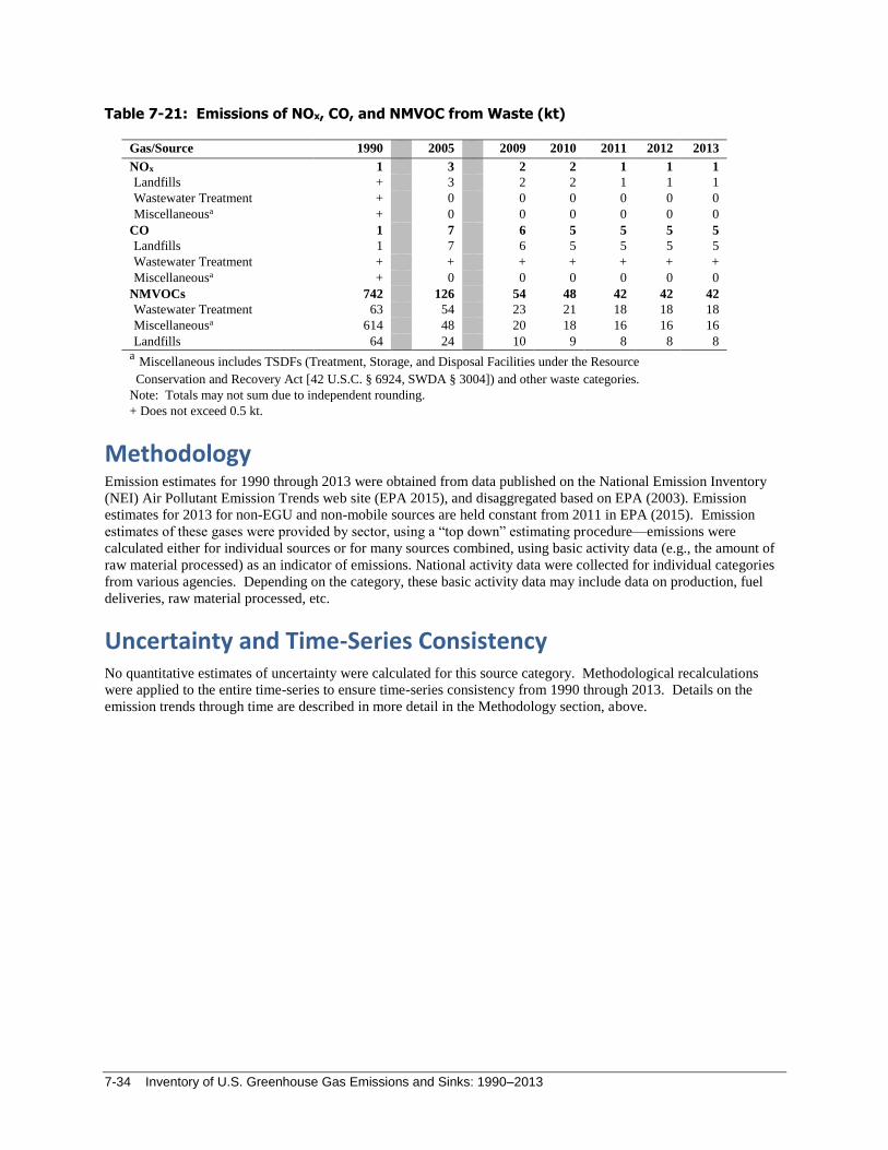
7-34 Inventory of U.S. Greenhouse Gas Emissions and Sinks: 1990–2013
Table 7-21: Emissions of NOx, CO, and NMVOC from Waste (kt)
Gas/Source 1990 2005 2009 2010 2011 2012 2013
NOx 1 3 2 2 1 1 1
Landfills + 3 2 2 1 1 1
Wastewater Treatment + 0 0 0 0 0 0
Miscellaneousa + 0 0 0 0 0 0
CO 1 7 6 5 5 5 5
Landfills 1 7 6 5 5 5 5
Wastewater Treatment + + + + + + +
Miscellaneousa + 0 0 0 0 0 0
NMVOCs 742 126 54 48 42 42 42 Wastewater Treatment 63 54 23 21 18 18 18
Miscellaneousa 614 48 20 18 16 16 16
Landfills 64 24 10 9 8 8 8
a Miscellaneous includes TSDFs (Treatment, Storage, and Disposal Facilities under the Resource
Conservation and Recovery Act [42 U.S.C. § 6924, SWDA § 3004]) and other waste categories. Note: Totals may not sum due to independent rounding.
+ Does not exceed 0.5 kt.
Methodology Emission estimates for 1990 through 2013 were obtained from data published on the National Emission Inventory
(NEI) Air Pollutant Emission Trends web site (EPA 2015), and disaggregated based on EPA (2003). Emission
estimates for 2013 for non-EGU and non-mobile sources are held constant from 2011 in EPA (2015). Emission
estimates of these gases were provided by sector, using a “top down” estimating procedure—emissions were
calculated either for individual sources or for many sources combined, using basic activity data (e.g., the amount of
raw material processed) as an indicator of emissions. National activity data were collected for individual categories
from various agencies. Depending on the category, these basic activity data may include data on production, fuel
deliveries, raw material processed, etc.
Uncertainty and Time-Series Consistency No quantitative estimates of uncertainty were calculated for this source category. Methodological recalculations
were applied to the entire time-series to ensure time-series consistency from 1990 through 2013. Details on the
emission trends through time are described in more detail in the Methodology section, above.

Other 8-1
8. Other The United States does not report any greenhouse gas emissions under the Intergovernmental Panel on Climate
Change (IPCC) “Other” sector.

Recalculations and Improvements 9-1
9. Recalculations and Improvements Each year, emission and sink estimates are recalculated and revised for all years in the Inventory of U.S. Greenhouse
Gas Emissions and Sinks, as attempts are made to improve both the analyses themselves, through the use of better
methods or data, and the overall usefulness of the report. In this effort, the United States follows the 2006 IPCC
Guidelines (IPCC 2006), which states, “Both methodological changes and refinements over time are an essential
part of improving inventory quality. It is good practice to change or refine methods” when: available data have
changed; the previously used method is not consistent with the IPCC guidelines for that category; a category has
become key; the previously used method is insufficient to reflect mitigation activities in a transparent manner; the
capacity for inventory preparation has increased; new inventory methods become available; and for correction of
errors.”
The results of all methodological changes and historical data updates made in the current Inventory report are
presented in this section; detailed descriptions of each recalculation are contained within each source’s description
found in this report, if applicable. Table 9-2 summarizes the quantitative effect of these changes on U.S. greenhouse
gas emissions and sinks and Table 9-3 summarizes the quantitative effect on annual net CO2 fluxes, both relative to
the previously published U.S. Inventory (i.e., the 1990 through 2012 report). These tables present the magnitude of
these changes in units of million metric tons of carbon dioxide equivalent (MMT CO2 Eq.).
The Recalculations Discussion section of each source’s description in the respective chapter of this Inventory
presents the details of each recalculation. In general, when methodological changes have been implemented, the
entire time series (i.e., 1990 through 2012) has been recalculated to reflect the change, per IPCC (2006). Changes in
historical data are generally the result of changes in statistical data supplied by other agencies.
For the current Inventory, emission estimates have been revised to reflect the GWPs provided in the IPCC Fourth
Assessment Report (AR4) (IPCC 2007). Revised UNFCCC reporting guidelines for national inventories now require
the use of GWP values from AR4 (IPCC 2007),298 which reflect an updated understanding of the atmospheric
properties of each greenhouse gas. AR4 GWP values differ from those presented in the IPCC Second Assessment
Report (SAR) (IPCC 1996) and used in the previous inventories as required by earlier UNFCCC reporting
guidelines. The use of AR4 GWP values in this Inventory results in time-series recalculations for most inventory
sources. In Table 9-1 below, recalculations are presented including both the quantitative effect of the data and
methodological changes as well as the quantitative effect of the change in using the AR4 GWP.
The following ten emission sources and sinks, which are listed in absolute decending order of the average change in
emissions or sequestration between 1990 and 2012, underwent some of the most significant methodological and
historical data changes. These emission sources consider only methodological and historical data changes. A brief
summary of the recalculations and/or improvements undertaken is provided for each of the ten sources.
Forest Land Remaining Forest Land (CO2 sink). Forest ecosystem stock and stock-change estimates differ from
the previous Inventory (EPA 2014) principally due to some changes in data and methods. The net effect of the
modifications was to slightly reduce net C uptake (i.e., lower sequestration) and C stocks from 1990 to the
present. The estimate of net annual change in HWP C stock and total C stock in HWP were revised upward by
small amounts. The increase in total net annual additions compared to estimates published in 2013 was 2 to 3
298 See <http://unfccc.int/resource/docs/2013/cop19/eng/10a03.pdf#page=2>.

9-2 Inventory of U.S. Greenhouse Gas Emissions and Sinks: 1990–2013
percent for 2010 through 2012. This increase was mostly due to changes in the amount of pulpwood used for
paper and composite panel products back to 2003. All the adjustments were made as a result of corrections in
the database of forest products statistics used to prepare the estimates (Howard forthcoming). These changes
resulted in an average annual increase of 76.7 MMT CO2 Eq. relative to the previous Inventory.
Agricultural Soil Management (N2O). Methodological recalculations in the current Inventory were associated
with the following improvements: 1) Driving the DAYCENT simulations with updated input data for the
excretion of C and N onto PRP and N additions from managed manure based on national livestock population
(note that revised total PRP N additions decreased from 4.4 to 4.1 MMT N on average and revised managed
manure additions decreased from 2.9 to 2.7 MMT N on average); 2) properly accounting for N inputs from
residues for crops not simulated by DAYCENT; (3) modifying the number of experimental study sites used to
quantify model uncertainty for direct N2O emissions and bias correction; and (4) reporting indirect N2O
emissions from forestland and settlements in their respective sections, instead of the agricultural soil
management section. These changes resulted in an average annual decrease of 43.6 MMT CO2 Eq. relative to
the previous Inventory.
Petrochemical Production (CO2). Emission information from EPA’s GHGRP was used to update estimates.
Average country-specific CO2 emission factors were derived from the 2010 through 2013 GHGRP data for
carbon black, ethylene, ethylene dichloride, and ethylene oxide. Annual production and CO2 emission factor
data were obtained from EPA’s GHGRP for 2010 through 2013, and were used to estimate emissions for 2010
through 2013. An average CO2 emission factor was calculated from the 2010 through 2013 GHGRP data and
was used to estimate emissions for 1990 through 2009 for carbon black, ethylene, ethylene dichloride, and
ethylene oxide using historic production data compiled for 1990 through 2009 (ACC 2014a; ACC 2014b). Note,
ethylene oxide is included in the IPCC petrochemical production source category but had not been included in
previous versions of this Inventory due to lack of publicly-available data. Similarly, acrylonitrile is included in
the IPCC Petrochemical Production source category but had not been included in the previous Inventory due to
lack of publicly-available data. Annual acrylonitrile production data for 1990 through 2013 was obtained from
ACC (ACC 2014b). These changes resulted in an average annual increase of 23.5 MMT CO2 Eq. relative to the
previous Inventory.
Landfills (CH4). Three major methodological recalculations were performed for the current Inventory. First, a
new SOG survey was published allowing for the update of the annual quantities of waste generated and
disposed and the amount of CH4 generated for the years 2009 through 2012. Second, the percent of the U.S.
population within the three precipitation ranges were updated for the year 2010 (see Table A-3 in Annex 3.14),
which impacted the distribution for the years 2001 through 2013 in the waste model. Third, the EPA’s GHGRP
CH4 recovery and destruction efficiency data were incorporated. These changes resulted in an average annual
increase of 18.9 MMT CO2 Eq. relative to the previous Inventory.
Petroleum Systems (CH4). For the current Inventory, EPA received information and data related to the emission
estimates through the Inventory preparation process, previous Inventories’ formal public notice periods, the
latest GHGRP data, and new studies. EPA carefully evaluated relevant information available, and made several
updates, such as updates to offshore platforms, pneumatic controllers, refineries, and well count data. In
addition, revisions to use the latest activity data resulted in changes to emissions for several sources. The
decrease in calculated emissions from this source is largely due to the recalculation for offshore platforms.
The net impact of the changes (comparing 2012 estimate from previous (2014) Inventory and current (2015)
Inventory) is a decrease in CH4 emissions of around 14.5 MMT CO2 Eq., or 38 percent. Recalculations in the
offshore petroleum platforms estimates resulted in a large decrease in the 2012 CH4 emission estimate from this
source in the production segment, from 15.2 MMT CO2 Eq. in the previous (2014) Inventory, to 4.7 MMT CO2
Eq. in the current (2015) Inventory. Recalculations to the onshore petroleum production emissions estimates
resulted in a small decrease in the 2012 CH4 emission estimate for onshore sources, from 22.0 MMT CO2 Eq. in
the 2014 Inventory, to 19.5 MMT CO2 Eq. in the 2015 Inventory. Methane emission estimates for other
segments (i.e., refining and transport) changed by around 0.5 percent.
Recalculations and Improvements 9-3
Across the 1990 through 2012 time series, compared to the previous (2014) Inventory, in the current (2015)
Inventory, the CH4 emission estimate decreased by 11.8 MMT CO2 Eq. on average.299
Fossil Fuel Combustion (CO2) The Energy Information Administration (EIA 2015) updated energy
consumption statistics across the time series relative to the previous Inventory. One such revision is the
historical petroleum consumption in the residential sector in 2011 and 2012. These revisions primarily impacted
the previous emission estimates from 2010 to 2012; however, additional revisions to industrial and
transportation petroleum consumption as well as industrial natural gas and coal consumption impacted emission
estimates across the time series. In addition, EIA revised the heat contents of motor gasoline, distillate fuel, and
petroleum coke.
For motor gasoline, heating values were previously based on the relative volumes of conventional and
reformulated gasoline in the total motor gasoline product supplied to the United States. The revised heating
values (first occurring in the January 2015 publication of the Monthly Energy Review) incorporated inputs of
ethanol, methyl tert-butyl ether (MTBE) through April 2006, other oxygenates through 2006, and a single
national hydrocarbon gasoline blend-stock from 1993 through 2013.
Changes to the heat content of distillate fuel resulted in an annual average decrease of approximately 0.1
percent between 1994 through 2012. This decrease was a result of EIA’s heat content revision from a constant
sulfur content across the time series, to a weighted sulfur content. Additionally, in 2009, EIA began subtracting
inputs of renewable diesel fuel from petroleum consumption before converting to energy units.
Petroleum coke consumption decreased by an annual average of approximately 0.1 percent from 2004 to 2012.
This decrease was a result of a similar heat content revision in which the EIA recalculated the historically
constant petroleum coke heat content to include weighted petroleum coke heat contents (by the two categories
of petroleum coke, catalyst and marketable) starting in 2004.
Overall, these changes resulted in an average annual decrease of 9.6 MMT CO2 Eq. (less than 0.2 percent) in
CO2 emissions from fossil fuel combustion for the period 1990 through 2012, relative to the previous report.
Nitric Acid Production (N2O). GHGRP data from subpart V of regulation 40 CFR Part 98 were used to
recalculate emissions from nitric acid production over the entire time series (EPA 2014), and used directly for
emission estimates for 2010 through 2013. Nitric acid production and N2O emissions data were available for
2010 through 2013 from EPA’s GHGRP, given nearly all nitric acid production facilities, with the exception of
the strong acid facility, in the United States are required to report annual data under subpart V. Country-specific
N2O emission factors were developed using the 2010 GHGRP emissions and production data for nitric acid
production with abatement and without abatement. Due to differences in operational efficiencies and recent
installation of abatement technology at some U.S. facilities, 2010 GHGRP production data were used for
recalculating time series emissions (1990 through 2009) instead of average factors developed from 2010
through 2013 GHGRP data. As per the 2010 GHGRP data, 70.7 percent of total domestic nitric acid production
was estimated to be produced without any abatement.
Time series emissions for 1990 through 2009 were recalculated, and the revised emission estimates are
approximately 30 percent lower than the prior estimates. Throughout the whole time series, these changes
resulted in an average annual decrease of 5.3 MMT CO2 Eq. relative to the previous Inventory.
Natural Gas Systems (CH4). For the current Inventory, EPA received information and data related to the
emission estimates through the Inventory preparation process, previous Inventories’ formal public notice
periods, GHGRP data, and new studies. EPA carefully evaluated relevant information available, and made
several updates, including revisions to offshore platforms, pneumatic controllers, well counts data, and
hydraulically fractured gas well completions and workovers.
In addition, revisions to activity data resulted in changes to emission estimates for several sources. For example,
the 2014 Inventory used 2011 data as a proxy for condensate production for 2012. The 2015 Inventory was
299 Additional information on recent changes to the Inventory can be found at:
<http://www.epa.gov/climatechange/ghgemissions/usinventoryreport/natural-gas-systems.html>.

9-4 Inventory of U.S. Greenhouse Gas Emissions and Sinks: 1990–2013
updated to use the most recent data on condensate production. Large increases in production in the Rocky
Mountain and Gulf Coast regions resulted in an increase in calculated 2012 CH4 emissions from condensate
tanks of 0.6 MMT CO2 Eq., or 15 percent.
The combined impact of all revisions on 2012 natural gas production segment emissions compared to the
previous (2014) Inventory, is a decrease in CH4 emissions of approximately 0.2 MMT CO2 Eq. Recalculations
in the offshore gas platforms estimates resulted in a large decrease in the 2012 CH4 emission estimate from this
source in the production segment, from 7.2 MMT CO2 Eq. in the previous (2014) Inventory, to 3.8 MMT CO2
Eq. in the current (2015) Inventory. Recalculations to the onshore gas production emissions estimates resulted
in an increase in the 2012 CH4 emission estimate for onshore sources, from 42.6 MMT CO2 Eq. in the previous
(2014) Inventory, to 46.0 MMT CO2 Eq. in the current (2015) Inventory. Methane emission estimates for other
segments (i.e. processing, transmission and storage, and distribution) changed by less than 0.5 percent.
Across the 1990-2012 time series, compared to the previous (2014) Inventory, in the current (2015) Inventory,
the total CH4 emission estimate decreased by 5.2 MMT CO2 Eq. on average (or 3 percent), with the largest
decreases in the estimate occurring in early years of the time series.300
Petroleum Systems (CO2). EPA received information and data related to the emission estimates through the
Inventory preparation process, previous Inventories’ formal public notice periods, the latest GHGRP data, and
new studies. EPA carefully evaluated relevant information available, and made several updates, such as updates
to offshore platforms, pneumatic controllers, refineries, and well count data. In addition, revisions to use the
latest activity data resulted in changes to emissions for several sources.
The net impact of the changes (comparing 2012 estimate from previous (2014) Inventory and current (2015)
Inventory) is an increase in CO2 emissions of around 6 MMT CO2, or 1,400 percent. The increase in the CO2
emission estimates is due to the update to the petroleum refineries calculations.
Across the 1990-2012 time series, compared to the previous (2014) Inventory, in the current (2015) Inventory,
the CO2 emissions estimate increased by 4.4 MMT CO2 Eq. on average (or around 1,300 percent).301
Cropland Remaining Cropland (CO2 sink). Recalculations for the cropland remaining cropland source is
divided up into three components: Refining parameters associated with simulating crop production and carbon
inputs to the soil in the DAYCENT biogeochemical model; improving the model simulation of snow melt and
water infiltration in soils; and driving the DAYCENT simulations with updated input data for managed manure
based on national livestock population. These changes resulted in an average annual decrease of 4.3 MMT CO2
Eq. relative to the previous Inventory.
300 Additional information on recent changes to the Inventory can be found at:
<http://www.epa.gov/climatechange/ghgemissions/usinventoryreport/natural-gas-systems.html.> 301 Additional information on recent changes to the Inventory can be found at:
http://www.epa.gov/climatechange/ghgemissions/usinventoryreport/natural-gas-systems.html.

Recalculations and Improvements 9-5
Table 9-1: Revisions to U.S. Greenhouse Gas Emissions, Including Quantitative Change
Related to Use of AR4 GWP values (MMT CO2 Eq.)
Gas/Source 1990 2005 2009 2010 2011 2012
Average
Annual
Change
CO2 15.0 21.7 (5.5) (17.8) (23.3) (24.9) 15.3
Fossil Fuel Combustion (4.4) (5.2) (28.7) (37.8) (39.8) (46.3) (9.6)
Electricity Generation NC (1.3) (0.8) (0.8) (0.8) (0.5) (0.4)
Transportation (0.2) (3.9) (27.4) (33.1) (36.3) (38.8) (8.2)
Industrial (2.6) 0.2 0.2 0.1 5.4 10.1 0.5
Residential NC (0.1) + (0.1) 2.3 (5.8) (0.1)
Commercial (1.6) (0.1) (0.4) (0.5) (0.5) (0.3) (0.3)
U.S. Territories NC + (0.3) (3.4) (9.8) (11.0) (1.1)
Non-Energy Use of Fuels (3.2) (2.1) (2.1) (6.3) (9.0) (5.4) (3.2)
Natural Gas Systems (0.1) + + + 0.5 (0.5) +
Cement Production NC NC NC NC NC NC NC
Lime Production 0.3 0.6 0.5 0.5 0.5 0.4 0.5
Other Process Uses of Carbonates NC NC NC NC NC + +
Glass Production NC NC NC NC NC + +
Soda Ash Production and Consumption NC NC NC NC NC NC NC
Carbon Dioxide Consumption 0.1 0.1 + (1.0) (1.0) (1.0) (0.1)
Incineration of Waste NC NC (0.4) (1.0) (1.6) (1.8) (0.2)
Titanium Dioxide Production NC NC NC NC NC (0.2) +
Aluminum Production NC NC NC NC NC NC NC
Iron and Steel Production & Metallurgical Coke
Production NC NC NC NC NC + +
Ferroalloy Production NC NC NC NC 0.1 0.2 +
Ammonia Production NC NC NC NC (0.1) + +
Urea Consumption for Non-Agricultural Purposes NC NC + + + (0.8) +
Phosphoric Acid Production + + + + + + +
Petrochemical Production 18.2 23.8 20.9 23.9 22.9 23.0 23.5
Silicon Carbide Production and Consumption NC NC NC NC NC NC NC
Lead Production NC NC NC NC NC NC NC
Zinc Production NC NC NC NC + 0.1 +
Liming of Agricultural Soils NC NC NC NC NC 1.8 0.1
Peatlands Remaining Peatlands + + (0.1) + + + +
Petroleum Systems 4.1 4.6 4.3 3.8 4.1 4.7 4.4
Magnesium Production and Processing NC* NC* NC* NC* NC* NC* NC*
Urea Fertilization NC NC NC + 0.1 0.8 +
Land Use, Land-Use Change, and Forestry (Sink)a 55.3 118.8 90.7 96.4 99.3 98.9 72.2
Biomass – Wooda NC NC NC NC NC 0.9 +
International Bunker Fuelsa NC NC NC NC NC NC NC
Biomass – Ethanola NC NC NC NC NC NC NC
CH4 109.8 122.1 113.0 81.6 82.6 80.4 111.7
Stationary Combustion 1.0 0.8 0.7 0.7 0.7 0.9 0.9
Mobile Combustion 1.1 0.6 0.5 0.5 0.5 0.5 0.8
Coal Mining 15.4 10.5 12.8 13.2 11.4 10.6 11.9
Abandoned Underground Coal Mines 1.2 1.1 1.2 1.6 1.6 1.5 1.3
Natural Gas Systems 22.7 24.3 25.1 24.9 26.1 24.5 23.9
Petroleum Systems (4.2) (5.4) (7.6) (8.2) (8.6) (8.5) (5.8)
Petrochemical Production (2.0) (3.0) (2.8) (3.0) (3.1) (3.0) (2.8)
Silicon Carbide Production and Consumption + + + + + + +
Iron and Steel Production & Metallurgical Coke
Production 0.2 0.1 0.1 0.1 0.1 0.1 0.2
Ferroalloy Production + + + + + + +

9-6 Inventory of U.S. Greenhouse Gas Emissions and Sinks: 1990–2013
Enteric Fermentation 26.3 26.4 26.6 26.2 25.8 25.3 26.7
Manure Management 5.7 8.8 9.2 9.1 9.4 10.8 7.9
Rice Cultivation 1.5 1.4 1.5 1.8 1.4 1.9 1.5
Field Burning of Agricultural Residues 0.1 + + + + + +
Forest Fires + 0.2 0.1 + 0.6 0.4 0.2
Peatlands Remaining Peatlands NC NC NC NC NC NC NC
Landfills 38.5 53.4 42.8 11.9 13.9 12.4 42.2
Wastewater Treatment 2.5 2.5 2.5 2.5 2.4 2.4 2.6
Composting 0.1 0.3 0.3 0.3 0.3 0.3 0.2
Incineration of Waste + + + + + + +
International Bunker Fuelsa + + + + + + +
N2O (68.7) (59.9) (56.1) (49.3) (45.3) (44.5) (63.4)
Stationary Combustion (0.3) (0.4) (0.3) (0.4) (0.3) (0.6) (0.4)
Mobile Combustion (2.8) 1.2 1.9 3.0 4.0 3.7 (0.4)
Adipic Acid Production (0.6) (0.3) (0.1) (0.2) (0.4) (0.2) (0.3)
Nitric Acid Production (6.0) (5.6) (4.4) (5.2) (5.0) (4.8) (6.0)
Manure Management (0.6) (0.7) (0.7) (0.7) (0.7) (0.7) (0.6)
Agricultural Soil Management (58.1) (53.7) (52.3) (45.8) (42.0) (40.6) (55.2)
Field Burning of Agricultural Residues + + + + + + +
Wastewater Treatment (0.1) (0.1) (0.2) (0.2) (0.2) (0.2) (0.1)
N2O from Product Uses (0.2) (0.2) (0.2) (0.2) (0.2) (0.2) (0.2)
Incineration of Waste + + + + (0.1) (0.1) +
Settlement Soils 0.4 0.9 0.8 0.9 1.0 1.1 0.8
Forest Fires (0.4) (1.1) (0.9) (0.7) (1.8) (2.1) (1.0)
Forest Soils + 0.1 0.1 0.1 0.1 0.1 0.1
Composting + (0.1) (0.1) (0.1) (0.1) + +
Peatlands Remaining Peatlands + + + + + + +
Semiconductor Manufacture NC* NC* NC* NC* NC* NC* NC*
International Bunker Fuelsa + + + + + + +
HFCs 9.7 11.6 7.8 8.6 8.8 8.0 11.9
Substitution of Ozone Depleting Substances + 7.3 6.4 6.9 6.9 6.8 5.9
HCFC-22 Production 9.7 4.2 1.4 1.7 1.8 1.1 6.0
Semiconductor Manufacture + + + + + + 0.1
Magnesium Production and Processing NC* NC* NC* NC* NC* NC* NC*
PFCs 3.6 1.1 0.6 0.7 0.9 0.6 2.0
Aluminum Production 3.0 0.5 0.3 0.3 0.5 0.4 1.2
Semiconductor Manufacture 0.6 0.6 0.3 0.4 0.4 0.1 0.8
SF6 (1.6) (0.6) (0.3) (0.3) (0.8) (0.7) (0.9)
Electrical Transmission and Distribution (1.3) (0.5) (0.2) (0.2) (0.4) (0.3) (0.7)
Semiconductor Manufacture + + + + (0.3) (0.3) (0.1)
Magnesium Production and Processing (0.3) (0.1) (0.1) (0.1) (0.1) (0.1) (0.2)
NF3 NC* NC* NC* NC* NC* NC* NC*
Semiconductor Manufacture NC* NC* NC* NC* NC* NC* NC*
Net Change in Total Emissionsb 67.8 96.4 59.9 24.1 23.6 19.5
Percent Change 1.1% 1.3% 0.9% 0.4% 0.4% 0.3%
Note: Emissions values are presented in CO2 equivalent mass units using IPCC AR4 GWP values.
Note: Totals may not sum due to independent rounding. Parentheses indicate negative values.
NC (No Change)
+ Absolute value does not exceed 0.05 MMT CO2 Eq. or 0.05 percent
* Indicates a new source for the current Inventory year a Not included in emissions total. b Excludes net CO2 flux from Land Use, Land-Use Change, and Forestry, and emissions from International
Bunker Fuels.

Recalculations and Improvements 9-7
Table 9-2: Revisions to U.S. Greenhouse Gas Emissions due only to Methodology and Data
Changes, with the AR4 GWP values applied across the time series (MMT CO2 Eq.)
Gas/Source 1990 2005 2009 2010 2011 2012
Average
Annual
Change
CO2 15.0 21.7 (5.5) (17.8) (23.3) (24.9) 15.3
Fossil Fuel Combustion (4.4) (5.2) (28.7) (37.8) (39.8) (46.3) (9.6)
Electricity Generation NC (1.3) (0.8) (0.8) (0.8) (0.5) (0.4)
Transportation (0.2) (3.9) (27.4) (33.1) (36.3) (38.8) (8.2)
Industrial (2.6) 0.2 0.2 0.1 5.4 10.1 0.5
Residential NC (0.1) + (0.1) 2.3 (5.8) (0.1)
Commercial (1.6) (0.1) (0.4) (0.5) (0.5) (0.3) (0.3)
U.S. Territories NC + (0.3) (3.4) (9.8) (11.0) (1.1)
Non-Energy Use of Fuels (3.2) (2.1) (2.1) (6.3) (9.0) (5.4) (3.2)
Natural Gas Systems (0.1) + + + 0.5 (0.5) +
Cement Production NC NC NC NC NC NC NC
Lime Production 0.3 0.6 0.5 0.5 0.5 0.4 0.5
Other Process Uses of Carbonates NC NC NC NC NC + +
Glass Production NC NC NC NC NC + +
Soda Ash Production and Consumption NC NC NC NC NC NC NC
Carbon Dioxide Consumption 0.1 0.1 + (1.0) (1.0) (1.0) (0.1)
Incineration of Waste NC NC (0.4) (1.0) (1.6) (1.8) (0.2)
Titanium Dioxide Production NC NC NC NC NC (0.2) +
Aluminum Production NC NC NC NC NC NC NC
Iron and Steel Production & Metallurgical Coke
Production NC NC NC NC NC + +
Ferroalloy Production NC NC NC NC 0.1 0.2 +
Ammonia Production NC NC NC NC (0.1) + +
Urea Consumption for Non-Agricultural Purposes NC NC + + + (0.8) +
Phosphoric Acid Production + + + + + + +
Petrochemical Production 18.2 23.8 20.9 23.9 22.9 23.0 23.5
Silicon Carbide Production and Consumption NC NC NC NC NC NC NC
Lead Production NC NC NC NC NC NC NC
Zinc Production NC NC NC NC + 0.1 +
Liming of Agricultural Soils NC NC NC NC NC 1.8 0.1
Peatlands Remaining Peatlands + + (0.1) + + + +
Petroleum Systems 4.1 4.6 4.3 3.8 4.1 4.7 4.4
Magnesium Production and Processing NC* NC* NC* NC* NC* NC* NC*
Urea Fertilization NC NC NC + 0.1 0.8 +
Land Use, Land-Use Change, and Forestry (Sink)a 55.3 118.8 90.7 96.4 99.3 98.9 NC
Biomass – Wooda NC NC NC NC NC 0.9 +
International Bunker Fuelsa NC NC NC NC NC NC NC
Biomass – Ethanola NC NC NC NC NC NC NC
CH4 (11.3) 10.5 (0.7) (29.9) (27.5) (27.7) (3.7)
Stationary Combustion (0.4) (0.5) (0.5) (0.5) (0.5) (0.2) (0.4)
Mobile Combustion 0.2 0.2 0.1 0.2 0.2 0.2 0.2
Coal Mining NC 0.3 NC NC NC NC +
Abandoned Underground Coal Mines NC NC 0.3 0.6 0.7 0.6 0.1
Natural Gas Systems (7.1) (4.7) (2.1) (0.8) 0.7 (0.2) (5.2)
Petroleum Systems (11.1) (10.9) (13.2) (13.8) (14.4) (14.5) (11.8)
Petrochemical Production (2.5) (3.6) (3.4) (3.6) (3.7) (3.6) (3.4)
Silicon Carbide Production and Consumption NC NC NC NC NC NC NC
Iron and Steel Production & Metallurgical Coke
Production NC NC NC NC NC NC NC
Ferroalloy Production NC NC NC NC + + +

9-8 Inventory of U.S. Greenhouse Gas Emissions and Sinks: 1990–2013
Enteric Fermentation NC (0.7) (1.2) (1.4) (1.5) (1.5) (0.7)
Manure Management (0.3) (0.3) (0.4) (0.7) (0.5) 0.7 (0.3)
Rice Cultivation NC NC NC NC NC 0.5 +
Field Burning of Agricultural Residues NC NC NC NC NC NC NC
Forest Fires (0.5) (1.4) (1.0) (0.9) (2.0) (2.5) (1.2)
Peatlands Remaining Peatlands NC NC NC NC NC NC NC
Landfills 10.3 32.0 20.8 (9.0) (6.5) (7.2) 18.9
Wastewater Treatment + + + + + + +
Composting NC NC NC NC + + +
Incineration of Waste NC NC + + + + +
International Bunker Fuelsa NC NC NC NC NC NC NC
N2O (53.3) (43.8) (40.2) (33.4) (29.2) (28.6) (47.1)
Stationary Combustion 0.1 0.4 0.5 0.5 0.5 0.2 0.3
Mobile Combustion (1.1) 2.6 2.8 3.8 4.7 4.3 1.2
Adipic Acid Production NC NC NC NC NC + +
Nitric Acid Production (5.3) (5.0) (3.8) (4.5) (4.3) (4.2) (5.3)
Manure Management NC NC + + + + +
Agricultural Soil Management (47.2) (42.2) (40.0) (33.8) (30.0) (28.8) (43.6)
Field Burning of Agricultural Residues NC NC NC NC NC NC NC
Wastewater Treatment + + + + + + +
N2O from Product Uses NC NC NC NC NC NC NC
Incineration of Waste NC NC + + + + +
Settlement Soils 0.4 0.9 0.9 0.9 1.0 1.1 0.8
Forest Fires (0.3) (0.9) (0.7) (0.6) (1.3) (1.7) (0.8)
Forest Soils 0.1 0.1 0.1 0.1 0.1 0.1 0.1
Composting NC NC NC NC + + +
Peatlands Remaining Peatlands + + + + + + +
Semiconductor Manufacture NC* NC* NC* NC* NC* NC* NC*
International Bunker Fuelsa NC NC NC NC NC NC NC
HFCs + (1.6) (5.5) (6.3) (7.1) (8.3) (0.9)
Substitution of Ozone Depleting Substances + (1.6) (5.5) (6.3) (7.1) (8.3) (0.9)
HCFC-22 Production NC NC NC NC NC NC NC
Semiconductor Manufacture NC + + + + + +
Magnesium Production and Processing NC* NC* NC* NC* NC* NC* NC*
PFCs + (0.5) (0.5) (0.5) (0.7) (0.9) (0.3)
Aluminum Production NC NC NC NC NC NC NC
Semiconductor Manufacture + (0.5) (0.5) (0.5) (0.7) (0.9) (0.3)
SF6 (0.1) + 0.1 0.1 (0.3) (0.3) +
Electrical Transmission and Distribution (0.1) + 0.2 0.1 + + +
Semiconductor Manufacture NC + + + (0.2) (0.2) +
Magnesium Production and Processing NC NC + + + + +
NF3 NC* NC* NC* NC* NC* NC* NC*
Semiconductor Manufacture NC* NC* NC* NC* NC* NC* NC*
Net Change in Total Emissionsb (49.6) (13.1) (51.8) (87.3) (87.4) (90.1)
Percent Change -0.8% -0.2% -0.8% -1.2% -1.3% -1.4%
Note: Emissions values are presented in CO2 equivalent mass units using IPCC AR4 GWP values.
Note: Totals may not sum due to independent rounding. Parentheses indicate negative values.
+ Absolute value does not exceed 0.05 MMT CO2 Eq. or 0.05 percent
NC (No Change)
* Indicates a new source for the current Inventory year a Not included in emissions total. b Excludes net CO2 flux from Land Use, Land-Use Change, and Forestry, and emissions from International
Bunker Fuels.

Recalculations and Improvements 9-9
Table 9-3: Revisions to Annual Sinks (C Sequestration) from Land Use, Land-Use Change,
and Forestry (MMT CO2 Eq.)
Component: Sinks from Land Use,
Land-Use Change, and Forestrya 1990 2005 2009 2010 2011 2012
Average
Annual
Change
Forest Land Remaining Forest Land:
Changes in Forest Carbon Stock 65.1 120.2 84.5 90.2 93.2 93.4 76.7
Cropland Remaining Cropland:
Changes in Agricultural Soil Carbon
Stock (13.3) 1.1 1.8 1.8 1.8 1.5 (4.3)
Land Converted to Cropland (2.4) (1.0) (0.6) (0.6) (0.6) (0.7) (1.0)
Grassland Remaining Grassland 7.6 (1.4) 4.9 4.9 4.9 4.8 1.8
Land Converted to Grassland (0.1) (0.7) (0.3) (0.3) (0.3) (0.2) (0.2)
Settlements Remaining Settlements:
Changes in Urban Tree Carbon
Stock NC NC NC NC NC NC NC
Other (Landfilled Yard Trimmings and
Food Scraps) (1.8) 0.6 0.4 0.4 0.3 0.3 (0.7)
Net Change in Sinksa 55.3 118.8 90.7 96.4 99.3 98.9
Percent Change 6.7% 11.5% 9.4% 10.0% 10.1% 10.1%
NC (No Change)
Note: Numbers in parentheses indicate an increase in C sequestration. a The sinks value includes the positive C sequestration reported for Forest Land Remaining Forest
Land, Cropland Remaining Cropland, Land Converted to Grassland, Settlements Remaining
Settlements, and Other Land plus the loss in C sequestration reported for Land Converted to
Cropland and Grassland Remaining Grassland.
Note: Totals may not sum due to independent rounding.

References 10-1
10. References
Executive Summary BEA (2014) 2014 Comprehensive Revision of the National Income and Product Accounts: Current-dollar and
"real" GDP, 1929–2013. Bureau of Economic Analysis (BEA), U.S. Department of Commerce, Washington, D.C.
Last Modified November 2014. Available online at <http://www.bea.gov/national/index.htm#gdp>.
EIA (2015a) Electricity Generation. Monthly Energy Review, February 2015. Energy Information Administration,
U.S. Department of Energy, Washington, D.C. DOE/EIA-0035(2015/02).
EIA (2015b) Electricity in the United States. Electricity Explained. Energy Information Administration, U.S.
Department of Energy, Washington, D.C. Available online at
<http://www.eia.gov/energyexplained/index.cfm?page=electricity_in_the_united_states>.
EIA (2013) International Energy Statistics 2013. Energy Information Administration (EIA), U.S. Department of
Energy. Washington, D.C. Available online at
<http://tonto.eia.doe.gov/cfapps/ipdbproject/IEDIndex3.cfm> EIA (2014). Accessed on 30 November 2014.
EPA (2015) “1970 - 2014 Average annual emissions, all criteria pollutants in MS Excel.” National Emissions
Inventory (NEI) Air Pollutant Emissions Trends Data. Office of Air Quality Planning and Standards. Last Modified
March 2015. Available online at <http://www.epa.gov/ttn/chief/trends/index.html>.
IPCC (2013) Climate Change 2013: The Physical Science Basis. Contribution of Working Group I to the Fifth
Assessment Report of the Intergovernmental Panel on Climate Change. [Stocker, T.F., D. Qin, G.-K., Plattner, M.
Tignor, S.K. Allen, J. Boschung, A. Nauels, Y. Xia, V. Bex and P.M. Midgley (eds.)]. Cambridge University Press,
Cambridge, United Kingdom and New York, NY, USA, 1535 pp.
IPCC (2007) Climate Change 2007: The Physical Science Basis. Contribution of Working Group I to the Fourth
Assessment Report of the Intergovernmental Panel on Climate Change. S. Solomon, D. Qin, M. Manning, Z. Chen,
M. Marquis, K.B. Averyt, M. Tignor and H.L. Miller (eds.). Cambridge University Press. Cambridge, United
Kingdom 996 pp.
IPCC (2006) 2006 IPCC Guidelines for National Greenhouse Gas Inventories. The National Greenhouse Gas
Inventories Programme, The Intergovernmental Panel on Climate Change. H.S. Eggleston, L. Buendia, K. Miwa, T.
Ngara, and K. Tanabe (eds.). Hayama, Kanagawa, Japan.
IPCC (2001) Climate Change 2001: The Scientific Basis. Intergovernmental Panel on Climate Change. J.T.
Houghton, Y. Ding, D.J. Griggs, M. Noguer, P.J. van der Linden, X. Dai, C.A. Johnson, and K. Maskell (eds.).
Cambridge University Press. Cambridge, United Kingdom.
IPCC (1996) Climate Change 1995: The Science of Climate Change. Intergovernmental Panel on Climate Change.
J.T. Houghton, L.G. Meira Filho, B.A. Callander, N. Harris, A. Kattenberg, and K. Maskell (eds.). Cambridge
University Press. Cambridge, United Kingdom.
NOAA/ESRL (2015) “Trends in Atmospheric Carbon Dioxide.” Available online at
<http://www.esrl.noaa.gov/gmd/ccgg/trends/>. 4 February 2015.

10-2 Inventory of U.S. Greenhouse Gas Emissions and Sinks: 1990–2013
UNFCCC (2014) Report of the Conference of the Parties on its nineteenth session, held in Warsaw from 11 to 23
November 2013. United Nations Framework Convention on Climate Change, Warsaw. (FCCC/CP/2013/10/Add.3).
January 31, 2014. Available online at <http://unfccc.int/resource/docs/2013/cop19/eng/10a03.pdf>.
U.S. Census Bureau (2014) U.S. Census Bureau International Database (IDB). November 2014. Available online at
<http://www.census.gov/ipc/www/idbnew.html>.
Introduction CDIAC (2014) Recent Greenhouse Gas Concentrations. T.J. Blasing; DOI: 10.3334/CDIAC/atg.032. Available
online at <http://cdiac.ornl.gov/pns/current_ghg.html>. 11 November 2014.
EPA (2009) Technical Support Document for the Endangerment and Cause or Contribute Findings for Greenhouse
Gases Under Section 202(a) of the Clean Air Act. U.S. Environmental Protection Agency. December 2009.
IPCC (2013) Climate Change 2013: The Physical Science Basis. Contribution of Working Group I to the Fifth
Assessment Report of the Intergovernmental Panel on Climate Change [Stocker, T.F., D. Qin, G.-K. Plattner, M.
Tignor, S.K. Allen, J. Boschung, A. Nauels, Y. Xia, V. Bex and P.M. Midgley (eds.)]. Cambridge University Press,
Cambridge, United Kingdom and New York, NY, USA, 1535 pp.
IPCC (2007) Climate Change 2007: The Physical Science Basis. Contribution of Working Group I to the Fourth
Assessment Report of the Intergovernmental Panel on Climate Change. S. Solomon, D. Qin, M. Manning, Z. Chen,
M. Marquis, K.B. Averyt, M. Tignor and H.L. Miller (eds.). Cambridge University Press. Cambridge, United
Kingdom 996 pp.
IPCC (2006) 2006 IPCC Guidelines for National Greenhouse Gas Inventories. The National Greenhouse Gas
Inventories Programme, The Intergovernmental Panel on Climate Change. H.S. Eggleston, L. Buendia, K. Miwa, T.
Ngara, and K. Tanabe (eds.). Hayama, Kanagawa, Japan.
IPCC (2001) Climate Change 2001: The Scientific Basis. Intergovernmental Panel on Climate Change. J.T.
Houghton, Y. Ding, D.J. Griggs, M. Noguer, P.J. van der Linden, X. Dai, C.A. Johnson, and K. Maskell (eds.).
Cambridge University Press. Cambridge, United Kingdom.
IPCC (1999) Aviation and the Global Atmosphere. Intergovernmental Panel on Climate Change. J.E. Penner, et al.
(eds.). Cambridge University Press. Cambridge, United Kingdom.
IPCC/TEAP (2005) Special Report: Safeguarding the Ozone Layer and the Global Climate System, Chapter 4:
Refrigeration. 2005. Available online <http://www.auto-
ts.com/hcfc/technology%20option/Refrigeration/transport%20refrigeration.pdf>.
Jacobson, M.Z. (2001) “Strong Radiative Heating Due to the Mixing State of Black Carbon in Atmospheric
Aerosols.” Nature, 409:695-697.
NOAA (2014) Vital Signs of the Planet. Available online at <http://climate.nasa.gov/causes/>. 12 December 2014.
NOAA/ESRL (2015) Trends in Atmospheric Carbon Dioxide. Available online at
<http://www.esrl.noaa.gov/gmd/ccgg/trends/>. 6 February 2015.
UNEP/WMO (1999) Information Unit on Climate Change. Framework Convention on Climate Change. Available
online at <http://unfccc.int>.
UNFCCC (2014) Report of the Conference of the Parties on its nineteenth session, held in Warsaw from 11 to 23
November 2013. United Nations Framework Convention on Climate Change, Warsaw. (FCCC/CP/2013/10/Add.3).
January 31, 2014. Available online at < http://unfccc.int/resource/docs/2013/cop19/eng/10a03.pdf>

References 10-3
Trends in Greenhouse Gas Emissions BEA (2014) 2013 Comprehensive Revision of the National Income and Product Accounts: Current-dollar and
"real" GDP, 1929–2013. Bureau of Economic Analysis (BEA), U.S. Department of Commerce, Washington, D.C.
Available online at <http://www.bea.gov/national/index.htm#gdp>.
Duffield, J. (2006) Personal communication. Jim Duffield, Office of Energy Policy and New Uses, USDA and
Lauren Flinn, ICF International. December 2006.
EIA (2015) Monthly Energy Review, February 2015. Energy Information Administration, U.S. Department of
Energy, Washington, D.C. DOE/EIA-0035(2015/02).
EPA (2015) “1970 - 2014 Average annual emissions, all criteria pollutants in MS Excel.” National Emissions
Inventory (NEI) Air Pollutant Emissions Trends Data. Office of Air Quality Planning and Standards, March 2015.
Available online at <http://www.epa.gov/ttn/chief/trends/index.html>.
EPA (2014) Light-Duty Automotive Technology, Carbon Dioxide Emissions, and Fuel Economy Trends: 1975 -
2014. Office of Transportation and Air Quality, U.S. Environmental Protection Agency. Available online at <
http://www.epa.gov/otaq/fetrends-complete.htm >.
FRB (2014) Industrial Production and Capacity Utilization. Federal Reserve Statistical Release, G.17, Federal
Reserve Board. Available online at <http://www.federalreserve.gov/releases/G17/table1_2.htm>. March 28, 2014.
IPCC (2006) 2006 IPCC Guidelines for National Greenhouse Gas Inventories. The National Greenhouse Gas
Inventories Programme, The Intergovernmental Panel on Climate Change. H.S. Eggleston, L. Buendia, K. Miwa, T.
Ngara, and K. Tanabe (eds.). Hayama, Kanagawa, Japan.
IPCC (2001) Climate Change 2001: The Scientific Basis. Intergovernmental Panel on Climate Change. J.T.
Houghton, Y. Ding, D.J. Griggs, M. Noguer, P.J. van der Linden, X. Dai, C.A. Johnson, and K. Maskell (eds.).
Cambridge University Press. Cambridge, United Kingdom.
U.S. Census Bureau (2014) U.S. Census Bureau International Database (IDB). Available online at
<http://www.census.gov/ipc/www/idbnew.html>.
Energy EIA (2013) Indicators: CO2 Emissions. International Energy Statistics 2013. Energy Information Administration,
U.S. Department of Energy. Washington, D.C. Available at
<http://tonto.eia.doe.gov/cfapps/ipdbproject/IEDIndex3.cfm>.
Carbon Dioxide Emissions from Fossil Fuel Combustion AAR (2008 through 2013) Railroad Facts. Policy and Economics Department, Association of American Railroads,
Washington, D.C. Obtained from Clyde Crimmel at AAR.
AISI (2004 through 2013) Annual Statistical Report, American Iron and Steel Institute, Washington, D.C.
APTA (2007 through 2013) Public Transportation Fact Book. American Public Transportation Association,
Washington, D.C. Available online at <http://www.apta.com/resources/statistics/Pages/transitstats.aspx>.
APTA (2006) Commuter Rail National Totals. American Public Transportation Association, Washington, D.C.
Available online at <http://www.apta.com/research/stats/rail/crsum.cfm>.
BEA (2014) Table 1.1.6. Real Gross Domestic Product, Chained 2009 Dollars. Bureau of Economic Analysis
(BEA), U.S. Department of Commerce, Washington, D.C. November, 2014. Available online at
<http://www.bea.gov/iTable/iTable.cfm?ReqID=9&step=1#reqid=9&step=3&isuri=1&904=1990&903=6&906=a&
905=2013&910=x&911=0>.

10-4 Inventory of U.S. Greenhouse Gas Emissions and Sinks: 1990–2013
Benson, D. (2002 through 2004) Unpublished data. Upper Great Plains Transportation Institute, North Dakota State
University and American Short Line & Regional Railroad Association.
Coffeyville Resources Nitrogen Fertilizers (2014) Nitrogen Fertilizer Operations. Available online at
<http://coffeyvillegroup.com/NitrogenFertilizerOperations/index.html>.
Dakota Gasification Company (2006) CO2 Pipeline Route and Designation Information. Bismarck, ND. Available
online at <http://www.dakotagas.com/SafetyHealth/Pipeline_Information.html>.
DHS (2008) Email Communication. Elissa Kay, Department of Homeland Security and Joe Aamidor, ICF
International. January 11, 2008.
DLA Energy (2014) Unpublished data from the Fuels Automated System (FAS). Defense Logistics Agency Energy,
U.S. Department of Defense. Washington, D.C.
DOC (1991 through 2013) Unpublished Report of Bunker Fuel Oil Laden on Vessels Cleared for Foreign Countries.
Form-563. Foreign Trade Division, Bureau of the Census, U.S. Department of Commerce. Washington, D.C.
DOE (1993 through 2014) Transportation Energy Data Book. Office of Transportation Technologies, Center for
Transportation Analysis, Energy Division, Oak Ridge National Laboratory. ORNL-6978.
DOE (2012) 2010 Worldwide Gasification Database. National Energy Technology Laboratory and Gasification
Technologies Council. Available online at
<http://www.netl.doe.gov/technologies/coalpower/gasification/worlddatabase/index.html>. Accessed on 15 March
2012.
DOT (1991 through 2013) Airline Fuel Cost and Consumption. U.S. Department of Transportation, Bureau of
Transportation Statistics, Washington, D.C. DAI-10. http://www.transtats.bts.gov/fuel.asp.
Eastman Gasification Services Company (2011) Project Data on Eastman Chemical Company’s Chemicals-from-
Coal Complex in Kingsport, TN. Available online at
<http://www.netl.doe.gov/coal/gasification/pubs/pdf/Eastman%20Chemicals%20from%20Coal%20Complex.pdf>.
EIA (2015) Monthly Energy Review, February 2015, Energy Information Administration, U.S. Department of
Energy, Washington, DC. DOE/EIA-0035(2015/2).
EIA (2014a) Natural Gas Annual 2013. Energy Information Administration, U.S. Department of Energy.
Washington, D.C. DOE/EIA-0131(06).
EIA (2014b) Quarterly Coal Report: January – March 2014. Energy Information Administration, U.S. Department
of Energy. Washington, D.C. DOE/EIA-0121.
EIA (2014c) U.S. Energy-Related Carbon Dioxide Emissions, 2013. Energy Information Administration, U.S.
Department of Energy. Washington, D.C. October 2014. Available online at
<http://www.eia.gov/environment/emissions/carbon/>.
EIA (1991 through 2014) Fuel Oil and Kerosene Sales. Energy Information Administration, U.S. Department of
Energy. Washington, D.C. Available online at: <http://www.eia.gov/petroleum/fueloilkerosene/>.
EIA (2013) Indicators: CO2 Emissions. International Energy Statistics 2013. Energy Information Administration,
U.S. Department of Energy. Washington, D.C. Available at:
<http://tonto.eia.doe.gov/cfapps/ipdbproject/IEDIndex3.cfm>.
EIA (2009a) Emissions of Greenhouse Gases in the United States 2008, Draft Report. Office of Integrated Analysis
and Forecasting, Energy Information Administration, U.S. Department of Energy. Washington, D.C. DOE-EIA-
0573(2009).
EIA (2009b) Manufacturing Consumption of Energy 2006. Energy Information Administration, U.S. Department of
Energy. Washington, D.C. Released July, 2009.
EIA (2008) Historical Natural Gas Annual, 1930 – 2008. Energy Information Administration, U.S. Department of
Energy. Washington, D.C.

References 10-5
EIA (2007) Personal Communication. Joel Lou, Energy Information Administration. and Aaron Beaudette, ICF
International. Residual and Distillate Fuel Oil Consumption for Vessel Bunkering (Both International and Domestic)
for American Samoa, U.S. Pacific Islands, and Wake Island. October 24, 2007.
EIA (2002) Alternative Fuels Data Tables. Energy Information Administration, U.S. Department of Energy.
Washington, D.C. Available online at <http://www.eia.doe.gov/fuelalternate.html>.
EIA (2001) U.S. Coal, Domestic and International Issues. Energy Information Administration, U.S. Department of
Energy. Washington, D.C. March 2001.
EPA (2014a) Acid Rain Program Dataset 1996-2013. Office of Air and Radiation, Office of Atmospheric Programs,
U.S. Environmental Protection Agency, Washington, D.C.
EPA (2014b). Motor Vehicle Emissions Simulator (Moves) 2014. Office of Transportation and Air Quality, U.S.
Environmental Protection Agency. Available online at < http://www.epa.gov/otaq/models/moves/index.htm>.
EPA (2014c) NONROAD 2008a Model. Office of Transportation and Air Quality, U.S. Environmental Protection
Agency. Available online at <http://www.epa.gov/oms/nonrdmdl.htm>.
EPA (2014d) Light-Duty Automotive Technology, Carbon Dioxide Emissions, and Fuel Economy Trends: 1975 -
2014. Office of Transportation and Air Quality, U.S. Environmental Protection Agency. Available online at <
http://www.epa.gov/otaq/fetrends-complete.htm >.
EPA (2010a) Carbon Content Coefficients Developed for EPA's Mandatory Reporting Rule. Office of Air and
Radiation, Office of Atmospheric Programs, U.S. Environmental Protection Agency, Washington, D.C.
Erickson, T. (2003) Plains CO2 Reduction (PCOR) Partnership. Presented at the Regional Carbon Sequestration
Partnership Meeting Pittsburgh, Pennsylvania, Energy and Environmental Research Center, University of North
Dakota. November 3, 2003. Available online at <http://www.netl.doe.gov/publications/proceedings/03/carbon-
seq/Erickson.pdf>.
FAA (2015) Personal Communication between FAA and Leif Hockstad for aviation emissions estimates from the
Aviation Environmental Design Tool (AEDT). January 2014.
FHWA (1996 through 2014) Highway Statistics. Federal Highway Administration, U.S. Department of
Transportation, Washington, D.C. Report FHWA-PL-96-023-annual. Available online at
<http://www.fhwa.dot.gov/policy/ohpi/hss/hsspubs.htm>.
Fitzpatrick, E. (2002) The Weyburn Project: A Model for International Collaboration. Available online at
<http://www.netl.doe.gov/coalpower/sequestration/pubs/mediarelease/mr-101102.pdf>.
FRB (2014) Industrial Production and Capacity Utilization. Federal Reserve Statistical Release, G.17, Federal
Reserve Board. Available online at <http://www.federalreserve.gov/releases/G17/table1_2.htm>. March 28, 2014.
Gaffney, J. (2007) Email Communication. John Gaffney, American Public Transportation Association and Joe
Aamidor, ICF International. December 17, 2007.
IPCC (2006) 2006 IPCC Guidelines for National Greenhouse Gas Inventories. The National Greenhouse Gas
Inventories Programme, The Intergovernmental Panel on Climate Change. H.S. Eggleston, L. Buendia, K. Miwa, T.
Ngara, and K. Tanabe (eds.). Hayama, Kanagawa, Japan.
Jacobs, G. (2010) Personal communication. Gwendolyn Jacobs, Energy Information Administration and Rubaab
Bhangu, ICF International. U.S. Territories Fossil Fuel Consumption, 1990–2013. Unpublished. U.S. Energy
Information Administration. Washington, D.C.
Marland, G. and A. Pippin (1990) “United States Emissions of Carbon Dioxide to the Earth’s Atmosphere by
Economic Activity.” Energy Systems and Policy, 14(4):323.
SAIC/EIA (2001) Monte Carlo Simulations of Uncertainty in U.S. Greenhouse Gas Emission Estimates. Final
Report. Prepared by Science Applications International Corporation (SAIC) for Office of Integrated Analysis and
Forecasting, Energy Information Administration, U.S. Department of Energy. Washington, D.C. June 22, 2001.
U.S. Census Bureau (2011) Current Industrial Reports Fertilizer Materials and Related Products: 2010 Summary.
Available online at <http://www.census.gov/manufacturing/cir/historical_data/mq325b/index.html>.

10-6 Inventory of U.S. Greenhouse Gas Emissions and Sinks: 1990–2013
USAA (2014) U.S. Primary Aluminum Production 2013. U.S. Aluminum Association, Washington, D.C. January,
2014.
USAF (1998) Fuel Logistics Planning. U.S. Air Force: AFPAM23-221. May 1, 1998.
United States Geological Survey (USGS) (1994 through 2011) Minerals Yearbook: Lead Annual Report. U.S.
Geological Survey, Reston, VA.
USGS (1991 through 2011) Minerals Yearbook: Manufactured Abrasives Annual Report. U.S. Geological Survey,
Reston, VA.
USGS (2011) 2010 Mineral Yearbook; Aluminum [Advanced Release]. U.S. Geological Survey, Reston, VA.
USGS (1991 through 2010a) Minerals Yearbook: Silicon Annual Report. U.S. Geological Survey, Reston, VA.
USGS (1991 through 2010b) Mineral Yearbook: Titanium Annual Report. U.S. Geological Survey, Reston, VA.
USGS (2010) 2009 Mineral Commodity Summaries: Aluminum. U.S. Geological Survey, Reston, VA.
USGS (2009) 2008 Mineral Yearbook: Aluminum. U.S. Geological Survey, Reston, VA.
USGS (2007) 2006 Mineral Yearbook: Aluminum. U.S. Geological Survey, Reston, VA.
USGS (1995, 1998, 2000 through 2002) Mineral Yearbook: Aluminum Annual Report. U.S. Geological Survey,
Reston, VA.
Whorton, D. (2006 through 2013) Personal communication, Class II and III Rail energy consumption, American
Short Line and Regional Railroad Association.
Stationary Combustion (excluding CO2) EIA (2015) Supplemental Tables on Petroleum Product detail. Monthly Energy Review, February 2015, Energy
Information Administration, U.S. Department of Energy, Washington, D.C. DOE/EIA-0035(2015/02).
EIA (2014) Electricity in the United States. Electricity Explained. Energy Information Administration, U.S.
Department of Energy, Washington, D.C. Available online at
<http://www.eia.gov/energyexplained/index.cfm?page=electricity_in_the_united_states>.
EPA (2015) “1970 - 2014 Average annual emissions, all criteria pollutants in MS Excel.” National Emissions
Inventory (NEI) Air Pollutant Emissions Trends Data. Office of Air Quality Planning and Standards. Available
online at <http://www.epa.gov/ttn/chief/trends/index.html>.
EPA (2014) NONROAD 2008a Model. Office of Transportation and Air Quality, U.S. Environmental Protection
Agency. Available online at <http://www.epa.gov/oms/nonrdmdl.htm>.
EPA (2003) E-mail correspondance. Air pollutant data. Office of Air Pollution to the Office of Air Quality Planning
and Standards, U.S. Environmental Protection Agency (EPA). December 22, 2003.
IPCC (2006) 2006 IPCC Guidelines for National Greenhouse Gas Inventories. The National Greenhouse Gas
Inventories Programme, The Intergovernmental Panel on Climate Change. H.S. Eggleston, L. Buendia, K. Miwa, T.
Ngara, and K. Tanabe (eds.). Hayama, Kanagawa, Japan.
Jacobs, G. (2010) Personal communication. Gwendolyn Jacobs, Energy Information Administration and Rubaab
Bhangu, ICF International. U.S. Territories Fossil Fuel Consumption, 1990–2009. Unpublished. U.S. Energy
Information Administration. Washington, D.C.
SAIC/EIA (2001) Monte Carlo Simulations of Uncertainty in U.S. Greenhouse Gas Emission Estimates. Final
Report. Prepared by Science Applications International Corporation (SAIC) for Office of Integrated Analysis and
Forecasting, Energy Information Administration, U.S. Department of Energy. Washington, D.C. June 22, 2001.
Mobile Combustion (excluding CO2) AAR (2008 through 2013) Railroad Facts. Policy and Economics Department, Association of American Railroads,
Washington, D.C. Obtained from Clyde Crimmel at AAR.

References 10-7
ANL (2006) Argonne National Laboratory (2006) GREET model Version 1.7. June 2006.
APTA (2007 through 2013) Public Transportation Fact Book. American Public Transportation Association,
Washington, D.C. Available online at <http://www.apta.com/resources/statistics/Pages/transitstats.aspx>.
APTA (2006) Commuter Rail National Totals. American Public Transportation Association, Washington, D.C.
Available online at <http://www.apta.com/research/stats/rail/crsum.cfm>.
Benson, D. (2002 through 2004) Personal communication. Unpublished data developed by the Upper Great Plains
Transportation Institute, North Dakota State University and American Short Line & Regional Railroad Association.
BEA (1991 through 2013) Unpublished BE-36 survey data. Bureau of Economic Analysis, U.S. Department of
Commerce. Washington, D.C.
Browning, L. (2015) “Methodology for Highway Vehicle Alternative Fuel GHG Estimates”. Technical Memo,
March 2015.Browning, L. (2009) Personal communication with Lou Browning, “Suggested New Emission Factors
for Marine Vessels.”, ICF International.
Browning, L. (2005) Personal communication with Lou Browning, Emission control technologies for diesel
highway vehicles specialist, ICF International.
Browning, L. (2003) “VMT Projections for Alternative Fueled and Advanced Technology Vehicles through 2025.”
13th CRC On-Road Vehicle Emissions Workshop. April 2003.
DHS (2008) Email Communication. Elissa Kay, Department of Homeland Security and Joe Aamidor, ICF
International. January 11, 2008.
DLA Energy (2014) Unpublished data from the Defense Fuels Automated Management System (DFAMS). Defense
Energy Support Center, Defense Logistics Agency, U.S. Department of Defense. Washington, D.C.
DOC (1991 through 2013) Unpublished Report of Bunker Fuel Oil Laden on Vessels Cleared for Foreign Countries.
Form-563. Foreign Trade Division, Bureau of the Census, U.S. Department of Commerce. Washington, D.C.
DOE (1993 through 2014) Transportation Energy Data Book. Office of Transportation Technologies, Center for
Transportation Analysis, Energy Division, Oak Ridge National Laboratory. ORNL-6978.
DOT (1991 through 2013) Airline Fuel Cost and Consumption. U.S. Department of Transportation, Bureau of
Transportation Statistics, Washington, D.C. DAI-10. Available online at: <http://www.transtats.bts.gov/fuel.asp.>.
EIA (2015). Monthly Energy Review, February 2015, Energy Information Administration, U.S. Department of
Energy, Washington, D.C. DOE/EIA-0035(2015/02).
EIA (1991 through 2014) Fuel Oil and Kerosene Sales. Energy Information Administration, U.S. Department of
Energy. Washington, D.C. Available at: http://www.eia.gov/petroleum/fueloilkerosene/
EIA (2007 through 2012) Natural Gas Annual. Energy Information Administration, U.S. Department of Energy,
Washington, D.C. DOE/EIA-0131(11).
EIA (2011) Annual Energy Review 2010. Energy Information Administration, U.S. Department of Energy,
Washington, D.C. DOE/EIA-0384(2011). October 19, 2011.
EIA (2008) "Table 3.1: World Petroleum Supply and Disposition." International Energy Annual. Energy
Information Administration, U.S. Department of Energy. Washington, D.C. Available online at
<http://www.eia.doe.gov/iea/pet.html>.
EIA (2007) Personal Communication. Joel Lou, Energy Information Administration and Aaron Beaudette, ICF
International. Residual and Distillate Fuel Oil Consumption for Vessel Bunkering (Both International and Domestic)
for American Samoa, U.S. Pacific Islands, and Wake Island. October 24, 2007.
EIA (2002) Alternative Fuels Data Tables. Energy Information Administration, U.S. Department of Energy,
Washington, D.C. Available online at <http://www.eia.doe.gov/fuelrenewable.html>.
EPA (2014a) Annual Certification Test Results Report. Office of Transportation and Air Quality, U.S.
Environmental Protection Agency. Available online at <http://www.epa.gov/otaq/crttst.htm>.

10-8 Inventory of U.S. Greenhouse Gas Emissions and Sinks: 1990–2013
EPA (2014b) Confidential Engine Family Sales Data Submitted To EPA By Manufacturers. Office of
Transportation and Air Quality, U.S. Environmental Protection Agency.
EPA (2014c). Motor Vehicle Emissions Simulator (Moves) 2014. Office of Transportation and Air Quality, U.S.
Environmental Protection Agency. Available online at <http://www.epa.gov/otaq/models/moves/index.htm>.
EPA (2014d) NONROAD 2008a Model. Office of Transportation and Air Quality, U.S. Environmental Protection
Agency. Available online at <http://www.epa.gov/oms/nonrdmdl.htm>.
EPA (2015) “1970 - 2014 Average annual emissions, all criteria pollutants in MS Excel.” National Emissions
Inventory (NEI) Air Pollutant Emissions Trends Data. Office of Air Quality Planning and Standards. Available
online at <http://www.epa.gov/ttn/chief/trends/index.html>.
EPA (2000) Mobile6 Vehicle Emission Modeling Software. Office of Mobile Sources, U.S. Environmental
Protection Agency, Ann Arbor, Michigan.
EPA (1999a) Emission Facts: The History of Reducing Tailpipe Emissions. Office of Mobile Sources. May 1999.
EPA 420-F-99-017. Available online at <http://www.epa.gov/oms/consumer/f99017.pdf>.
EPA (1999b) Regulatory Announcement: EPA's Program for Cleaner Vehicles and Cleaner Gasoline. Office of
Mobile Sources. December 1999. EPA420-F-99-051. Available online at <http://www.epa.gov/otaq/regs/ld-
hwy/tier-2/frm/f99051.pdf>.
EPA (1998) Emissions of Nitrous Oxide from Highway Mobile Sources: Comments on the Draft Inventory of U.S.
Greenhouse Gas Emissions and Sinks, 1990–1996. Office of Mobile Sources, Assessment and Modeling Division,
U.S. Environmental Protection Agency. August 1998. EPA420-R-98-009.
EPA (1997) Mobile Source Emission Factor Model (MOBILE5a). Office of Mobile Sources, U.S. Environmental
Protection Agency, Ann Arbor, Michigan.
EPA (1994a) Automobile Emissions: An Overview. Office of Mobile Sources. August 1994. EPA 400-F-92-007.
Available online at <http://www.epa.gov/otaq/consumer/05-autos.pdf>.
EPA (1994b) Milestones in Auto Emissions Control. Office of Mobile Sources. August 1994. EPA 400-F-92-014.
Available online at <http://www.epa.gov/otaq/consumer/12-miles.pdf>.
EPA (1993) Automobiles and Carbon Monoxide. Office of Mobile Sources. January 1993. EPA 400-F-92-005.
Available online at <http://www.epa.gov/otaq/consumer/03-co.pdf>.
Esser, C. (2003 through 2004) Personal Communication with Charles Esser, Residual and Distillate Fuel Oil
Consumption for Vessel Bunkering (Both International and Domestic) for American Samoa, U.S. Pacific Islands,
and Wake Island.
FAA (2015) Personal Communication between FAA and Leif Hockstad for aviation emissions estimates from the
Aviation Environmental Design Tool (AEDT). January 2014.
FHWA (1996 through 2014) Highway Statistics. Federal Highway Administration, U.S. Department of
Transportation, Washington, D.C. Report FHWA-PL-96-023-annual. Available online at
<http://www.fhwa.dot.gov/policy/ohpi/hss/hsspubs.htm>.
Gaffney, J. (2007) Email Communication. John Gaffney, American Public Transportation Association and Joe
Aamidor, ICF International. December 17, 2007.
ICF (2006a) Revised Gasoline Vehicle EFs for LEV and Tier 2 Emission Levels. Memorandum from ICF
International to John Davies, Office of Transportation and Air Quality, U.S. Environmental Protection Agency.
November 2006.
ICF (2006b) Revisions to Alternative Fuel Vehicle (AFV) Emission Factors for the U.S. Greenhouse Gas Inventory.
Memorandum from ICF International to John Davies, Office of Transportation and Air Quality, U.S. Environmental
Protection Agency. November 2006.
ICF (2004) Update of Methane and Nitrous Oxide Emission Factors for On-Highway Vehicles. Final Report to U.S.
Environmental Protection Agency. February 2004.

References 10-9
Lipman, T. and M. Delucchi (2002) “Emissions of Nitrous Oxide and Methane from Conventional and Alternative
Fuel Motor Vehicles.” Climate Change, 53:477-516.
Santoni, G., B. Lee, E. Wood, S. Herndon, R. Miake-Lye, S Wofsy, J. McManus, D. Nelson, M. Zahniser (2011)
Aircraft emissions of methane and nitrous oxide during the alternative aviation fuel experiment. Environ Sci
Technol. 2011 Aug 15; 45(16):7075-82.
U.S. Census Bureau (2000) Vehicle Inventory and Use Survey. U.S. Census Bureau, Washington, D.C. Database
CD-EC97-VIUS.
Unnasch, S., L. Browning, and E. Kassoy (2001) Refinement of Selected Fuel-Cycle Emissions Analyses, Final
Report to ARB.
Whorton, D. (2006 through 2013) Personal communication, Class II and III Rail energy consumption, American
Short Line and Regional Railroad Association.
Carbon Emitted from Non-Energy Uses of Fossil Fuels ACC (2014a) "U.S. Resin Production & Sales: 2013 vs. 2012,” American Chemistry Council. Available online at:
<http://www.americanchemistry.com/Jobs/EconomicStatistics/Plastics-Statistics/Production-and-Sales-Data-by-
Resin.pdf>.
ACC (2014b) “Guide to the Business of Chemistry, 2014,” American Chemistry Council.
ACC (2012) “Guide to the Business of Chemistry, 2012,” American Chemistry Council.
ACC (2003-2011) "PIPS Year-End Resin Statistics for 2010: Production, Sales and Captive Use.” Available online
at <http://www.americanchemistry.com/Jobs/EconomicStatistics/Plastics-Statistics/Production-and-Sales-Data-by-
Resin.pdf>.
Bank of Canada (2014) Financial Markets Department Year Average of Exchange Rates. Available online at
<http://www.bankofcanada.ca/stats/assets/pdf/nraa-2013.pdf>.
Bank of Canada (2013) Financial Markets Department Year Average of Exchange Rates. Available online at
<http://www.bankofcanada.ca/stats/assets/pdf/nraa-2012.pdf>.
Bank of Canada (2012) Financial Markets Department Year Average of Exchange Rates. Available online at
<http://www.bankofcanada.ca/stats/assets/pdf/nraa-2011.pdf>.
EIA (2015) Supplemental Tables on Petroleum Product detail. Monthly Energy Review, February 2015. Energy
Information Administration, U.S. Department of Energy, Washington, D.C. DOE/EIA-0035(2015/02).
EIA (2013) EIA Manufacturing Consumption of Energy (MECS) 2010. U.S. Department of Energy, Energy
Information Administration, Washington, D.C.
EIA (2010) EIA Manufacturing Consumption of Energy (MECS) 2006. U.S. Department of Energy, Energy
Information Administration, Washington, D.C.
EIA (2005) EIA Manufacturing Consumption of Energy (MECS) 2002. U.S. Department of Energy, Energy
Information Administration, Washington, D.C.
EIA (2001) EIA Manufacturing Consumption of Energy (MECS) 1998. U.S. Department of Energy, Energy
Information Administration, Washington, D.C.
EIA (1997) EIA Manufacturing Consumption of Energy (MECS) 1994. U.S. Department of Energy, Energy
Information Administration, Washington, D.C.
EIA (1994) EIA Manufacturing Consumption of Energy (MECS) 1991. U.S. Department of Energy, Energy
Information Administration, Washington, D.C.
EPA (2015a) “1970 - 2014 Average annual emissions, all criteria pollutants in MS Excel.” National Emissions
Inventory (NEI) Air Pollutant Emissions Trends Data. Office of Air Quality Planning and Standards, March 2015.
Available online at <http://www.epa.gov/ttn/chief/trends/index.html>.
10-10 Inventory of U.S. Greenhouse Gas Emissions and Sinks: 1990–2013
EPA (2015b). Resource Conservation and Recovery Act (RCRA) Info, Biennial Report, GM Form (Section 2-
Onsite Management) and WR Form.
EPA (2014a) Municipal Solid Waste in the United States: 2012 Facts and Figures. Office of Solid Waste and
Emergency Response, U.S. Environmental Protection Agency, Washington, D.C. Available online at
<http://www.epa.gov/epaoswer/non-hw/muncpl/msw99.htm>.
EPA (2014b) Chemical Data Access Tool (CDAT). U.S. Environmental Protection Agency, June 2014. Available
online at <http://java.epa.gov/oppt_chemical_search/>. Accessed January 2015.
EPA (2013a) Municipal Solid Waste in the United States: 2011 Facts and Figures. Office of Solid Waste and
Emergency Response, U.S. Environmental Protection Agency, Washington, D.C. Available online at
<http://www.epa.gov/epaoswer/non-hw/muncpl/msw99.htm>.
EPA (2013b). Resource Conservation and Recovery Act (RCRA) Info, Biennial Report, GM Form (Section 2-
Onsite Management) and WR Form.
EPA (2011) EPA's Pesticides Industry Sales and Usage, 2006 and 2007 Market Estimates. Available online at
<http://www.epa.gov/oppbead1/pestsales/. Accessed January 2012>.
EPA (2009) Biennial Reporting System (BRS) Database. U.S. Environmental Protection Agency, Envirofacts
Warehouse. Washington, D.C. Available online at <http://www.epa.gov/enviro/html/brs/>. Data for 2001-2007 are
current as of Sept. 9, 2009.
EPA (2004) EPA's Pesticides Industry Sales and Usage, 2000 and 2001 Market Estimates. Available online at
<http://www.epa.gov/oppbead1/pestsales/. Accessed September 2006>.
EPA (2002) EPA's Pesticides Industry Sales and Usage, 1998 and 1999 Market Estimates, table 3.6. Available
online at <http://www.epa.gov/oppbead1/pestsales/99pestsales/market_estimates1999.pdf>. Accessed July 2003.
EPA (2001) AP 42, Volume I, Fifth Edition. Chapter 11: Mineral Products Industry. Available online at
<http://www.epa.gov/ttn/chief/ap42/ch11/index.html>.
EPA (2000a) Biennial Reporting System (BRS). U.S. Environmental Protection Agency, Envirofacts Warehouse.
Washington, D.C. Available online at <http://www.epa.gov/enviro/html/brs/>.
EPA (2000b) Toxics Release Inventory, 1998. U.S. Environmental Protection Agency, Office of Environmental
Information, Office of Information Analysis and Access, Washington, D.C. Available online at
<http://www.epa.gov/triexplorer/chemical.htm>.
EPA (1999) EPA's Pesticides Industry Sales and Usage, 1996-1997 Market Estimates. Available online at
<http://www.epa.gov/oppbead1/pestsales/97pestsales/market_estimates1997.pdf>.
EPA (1998) EPA's Pesticides Industry Sales and Usage, 1994-1995 Market Estimates. Available online at
<http://www.epa.gov/oppbead1/pestsales/95pestsales/market_estimates1995.pdf>.
FEB (2013) Fiber Economics Bureau, as cited in C&EN (2013) Lackluster Year for Chemical Output: Production
stayed flat or dipped in most world regions in 2012. Chemical &Engineering News, American Chemical Society, 1
July. Available online at <http://www.cen-online.org>.
FEB (2012) Fiber Economics Bureau, as cited in C&EN (2012) Too Quiet After the Storm: After a rebound in 2010,
chemical production hardly grew in 2011. Chemical & Engineering News, American Chemical Society, 2 July.
Available online at <http://www.cen-online.org>.
FEB (2011) Fiber Economics Bureau, as cited in C&EN (2011) Output Ramps up in all Regions. Chemical
Engineering News, American Chemical Society, 4 July. Available online at <http://www.cen-online.org>.
FEB (2010) Fiber Economics Bureau, as cited in C&EN (2010) Output Declines in U.S., Europe. Chemical &
Engineering News, American Chemical Society, 6 July. Available online at <http://www.cen-online.org>.
FEB (2009) Fiber Economics Bureau, as cited in C&EN (2009) Chemical Output Slipped In Most Regions Chemical
& Engineering News, American Chemical Society, 6 July. Available online at <http://www.cen-online.org>.
FEB (2007) Fiber Economics Bureau, as cited in C&EN (2007) Gains in Chemical Output Continue. Chemical &
Engineering News, American Chemical Society. July 2, 2007. Available online at <http://www.cen-online.org>.

References 10-11
FEB (2005) Fiber Economics Bureau, as cited in C&EN (2005) Production: Growth in Most Regions Chemical &
Engineering News, American Chemical Society, 11 July. Available online at <http://www.cen-online.org>.
FEB (2003) Fiber Economics Bureau, as cited in C&EN (2003) Production Inches Up in Most Countries, Chemical
& Engineering News, American Chemical Society, 7 July. Available online at <http://www.cen-online.org>.
FEB (2001) Fiber Economics Bureau, as cited in ACS (2001) Production: slow gains in output of chemicals and
products lagged behind U.S. economy as a whole Chemical & Engineering News, American Chemical Society, 25
June. Available online at <http://pubs.acs.org/cen>.
Financial Planning Association (2006) Canada/US Cross-Border Tools: US/Canada Exchange Rates. Available
online at <http://www.fpanet.org/global/planners/US_Canada_ex_rates.cfm>. Accessed August 16, 2006.
Gosselin, Smith, and Hodge (1984) "Clinical Toxicology of Commercial Products." Fifth Edition, Williams &
Wilkins, Baltimore.
Huurman, J.W.F. (2006) Recalculation of Dutch Stationary Greenhouse Gas Emissions Based on Sectoral Energy
Statistics 1990-2002. Statistics Netherlands, Voorburg, The Netherlands.
IISRP (2003) "IISRP Forecasts Moderate Growth in North America to 2007" International Institute of Synthetic
Rubber Producers, Inc. New Release. Available online at <http://www.iisrp.com/press-releases/2003-Press-
Releases/IISRP-NA-Forecast-03-07.html>.
IISRP (2000) "Synthetic Rubber Use Growth to Continue Through 2004, Says IISRP and RMA" International
Institute of Synthetic Rubber Producers press release.
INEGI (2006) Producción bruta total de las unidades económicas manufactureras por Subsector, Rama, Subrama y
Clase de actividad. Available online at
<http://www.inegi.gob.mx/est/contenidos/espanol/proyectos/censos/ce2004/tb_manufacturas.asp>. Accessed August
15.
IPCC (2006) 2006 IPCC Guidelines for National Greenhouse Gas Inventories. The National Greenhouse Gas
Inventories Programme, The Intergovernmental Panel on Climate Change. H.S. Eggleston, L. Buendia, K. Miwa, T.
Ngara, and K. Tanabe (eds.). Hayama, Kanagawa, Japan.
Marland, G., and R.M. Rotty (1984) “Carbon dioxide emissions from fossil fuels: A procedure for estimation and
results for 1950-1982”, Tellus 36b:232-261.
NPRA (2002) North American Wax - A Report Card. Available online at
<http://www.npra.org/members/publications/papers/lubes/LW-02-126.pdf>.
RMA (2014) 2013 U.S. Scrap Tire Management Summary. Rubber Manufacturers Association, Washington, D.C.
November 2014.
RMA (2011) U.S. Scrap Tire Management Summary: 2005-2009. Rubber Manufacturers Association, Washington,
D.C. October 2011, updated September 2013.
RMA (2009) “Scrap Tire Markets: Facts and Figures – Scrap Tire Characteristics.” Available online at:
http://www.rma.org/scrap_tires/scrap_tire_markets/scrap_tire_characteristics/ Accessed 17 September 2009.
Schneider, S. (2007) E-mail between Shelly Schneider of Franklin Associates (a division of ERG) and Sarah
Shapiro of ICF International, January 10, 2007.
U.S. Census Bureau (2014) 2012 Economic Census. Available online at:
<http://www.census.gov/econ/census/schedule/whats_been_released.html>. Accessed November 2014.
U.S. Census Bureau (2009) Soap and Other Detergent Manufacturing: 2007. Available online at
<http://smpbff1.dsd.census.gov/TheDataWeb_HotReport/servlet/HotReportEngineServlet?emailname=vh@boc&fil
ename=mfg1.hrml&20071204152004.Var.NAICS2002=325611&forward=20071204152004.Var.NAICS2002>.
U.S. Census Bureau (2004) Soap and Other Detergent Manufacturing: 2002, Issued December 2004, EC02-31I-
325611 (RV). Available online at <http://www.census.gov/prod/ec02/ec0231i325611.pdf>.
U.S. Census Bureau (1999) Soap and Other Detergent Manufacturing: 1997, Available online at
<http://www.census.gov/epcd/www/ec97stat.htm>.

10-12 Inventory of U.S. Greenhouse Gas Emissions and Sinks: 1990–2013
U.S. International Trade Commission (1990-2014) “Interactive Tariff and Trade DataWeb: Quick Query.” Available
online at <http://dataweb.usitc.gov/>. Accessed November 2014.
Incineration of Waste ArSova, Ljupka, Rob van Haaren, Nora Goldstein, Scott M. Kaufman, and Nickolas J. Themelis (2008) “16th
Annual BioCycle Nationwide Survey: The State of Garbage in America” Biocycle, JG Press, Emmaus, PA.
December.
Bahor, B (2009) Covanta Energy’s public review comments re: Draft Inventory of U.S. Greenhouse Gas Emissions
and Sinks: 1990-2007. Submitted via email on April 9, 2009 to Leif Hockstad, U.S. EPA.
De Soete, G.G. (1993) “Nitrous Oxide from Combustion and Industry: Chemistry, Emissions and Control.” In A. R.
Van Amstel, (ed) Proc. of the International Workshop Methane and Nitrous Oxide: Methods in National Emission
Inventories and Options for Control, Amersfoort, NL. February 3-5, 1993.
Energy Recovery Council (2009) “2007 Directory of Waste-to-Energy Plants in the United States.” Accessed
September 29, 2009.
EPA (2007, 2008, 2011, 2013, 2014) Municipal Solid Waste in the United States: Facts and Figures. Office of Solid
Waste and Emergency Response, U.S. Environmental Protection Agency. Washington, D.C. Available online at
<http://www.epa.gov/osw/nonhaz/municipal/msw99.htm>.
EPA (2006) Solid Waste Management and Greenhouse Gases: A Life-Cycle Assessment of Emissions and Sinks.
Office of Solid Waste and Emergency Response, U.S. Environmental Protection Agency. Washington, D.C.
EPA (2000) Characterization of Municipal Solid Waste in the United States: Source Data on the 1999 Update.
Office of Solid Waste, U.S. Environmental Protection Agency. Washington, D.C. EPA530-F-00-024.
Goldstein, N. and C. Madtes (2001) “13th Annual BioCycle Nationwide Survey: The State of Garbage in America.”
BioCycles, JG Press, Emmaus, PA. December 2001.
IPCC (2006) 2006 IPCC Guidelines for National Greenhouse Gas Inventories. The National Greenhouse Gas
Inventories Programme, The Intergovernmental Panel on Climate Change. H.S. Eggleston, L. Buendia, K. Miwa, T.
Ngara, and K. Tanabe (eds.). Hayama, Kanagawa, Japan.
Kaufman, et al. (2004) “14th Annual BioCycle Nationwide Survey: The State of Garbage in America 2004”
Biocycle, JG Press, Emmaus, PA. January, 2004.
RMA (2014) “2013 U.S. Scrap Tire Management Summary.” Rubber Manufacturers Association. November 2014.
Available online at: <http://www.rma.org/download/scrap-tires/market-reports/US_STMarket2013.pdf>.
RMA (2012a) "Rubber FAQs." Rubber Manufacturers Association. Available online at <http://www.rma.org/about-
rma/rubber-faqs/>. Accessed 19 November 2014.
RMA (2012b) “Scrap Tire Markets: Facts and Figures – Scrap Tire Characteristics.” Available online at
<http://www.rma.org/scrap_tires/scrap_tire_markets/scrap_tire_characteristics/>. Accessed 18 January 2012.
RMA (2011) “U.S. Scrap Tire Management Summary 2005-2009.” Rubber Manufacturers Association. October
2011. Available online at: <http://www.rma.org/scrap_tires/scrap_tire_markets/2009_summary.pdf>.
RTI (2009) Updated Hospital/Medical/Infectious Waste Incinerator (HMIWI) Inventory Database. Memo dated July
6, 2009. Available online at: <http://www.epa.gov/ttnatw01/129/hmiwi/hmiwi_inventory.pdf>.
Schneider, S. (2007) E-mail between Shelly Schneider of Franklin Associates (a division of ERG) and Sarah
Shapiro of ICF International, January 10, 2007.
Simmons, et al. (2006) “15th Nationwide Survey of Municipal Solid Waste Management in the United States: The
State of Garbage in America.” BioCycle, JG Press, Emmaus, PA. April 2006.
van Haaren, Rob, Thermelis, N., and Goldstein, N. (2010) "The State of Garbage in America." BioCycle, October
2010. Volume 51, Number 10, pg. 16-23.

References 10-13
Coal Mining AAPG (1984) Coalbed Methane Resources of the United States. AAPG Studies in Geology Series #17.
CAR (2014) Project Database. Climate Action Reserve. Available at <http://www.climateactionreserve.org/>.
Consol (2014) Ruby Canyon Summary 2013. CONSOL Energy Inc. excel spreadsheet
Creedy, D.P. (1993) Chemosphere. Vol. 26, pp. 419-440.
EIA (2014) Annual Coal Report 1991-2013 (Formerly called Coal Industry Annual). Table 1. Energy Information
Administration, U.S. Department of Energy, Washington, D.C.
EPA (2014) Greenhouse Gas Reporting Program (GHGRP): Underground Coal Mines. Retrieved from
http://www.epa.gov/ghgreporting/ghgdata/reported/coalmines.html
EPA (2005) Surface Mines Emissions Assessment. U.S. Environmental Protection Agency Draft Report.
EPA (1996) Evaluation and Analysis of Gas Content and Coal Properties of Major Coal Bearing Regions of the
United States. U.S. Environmental Protection Agency. EPA/600/R-96-065.
GSA (2014) Well Records Database. Geological Survey of Alabama State Oil and Gas Board. Retrieved from
<http://www.gsa.state.al.us/ogb/database.aspx>.
IEA (2014) Key World Energy Statistics. Coal Production, International Energy Agency.
IPCC (2011) Use of Models and Facility-Level Data in Greenhouse Gas Inventories (Report of IPCC Expert
Meeting on Use of Models and Measurements in Greenhouse Gas Inventories 9-11 August 2010, Sydney, Australia)
eds: Eggleston H.S., Srivastava N., Tanabe K., Baasansuren J., Fukuda M., Pub. IGES, Japan 2011.
JWR (2014) Wells Intercepted 2013. Jim Walter Resources excel spreadsheet.
JWR (2010) No. 4 & 7 Mines General Area Maps. Walter Energy: Jim Walter Resources.
King, Brian (1994) Management of Methane Emissions from Coal Mines: Environmental, Engineering, Economic
and Institutional Implication of Options, Neil and Gunter Ltd., Halifax, March 1994.
MSHA (2014) Data Transparency at MSHA. Mine Safety and Health Administration. Retrieved from
<http://www.msha.gov>.
Mutmansky, Jan M. and Yanbei Wang (2000) “Analysis of Potential Errors in Determination of Coal Mine Annual
Methane Emissions.” Mineral Resources Engineering, 9(4). December 2000.
Saghafi, Abouna (2013) Estimation of fugitive emissions from open cut coal mining and measurable gas content,
13th Coal Operators' Conference, University of Wollongong, The Australian Institute of Mining and Metallurgy &
Mine Managers Association of Australia, 2013, 306-313.
USBM (1986) Results of the Direct Method Determination of the Gas Contents of U.S. Coal Basins. Circular 9067,
U.S. Bureau of Mines.
West Virginia Geological & Economic Survey (WVGES) (2014) Oil & Gas Production Data. Retrieved from
<http://www.wvgs.wvnet.edu/www/datastat/datastat.htm>.
Abandoned Underground Coal Mines EPA (2004) Methane Emissions Estimates & Methodology for Abandoned Coal Mines in the U.S. Draft Final
Report. Washington, D.C. April 2004.
Mutmansky, Jan M., and Yanbei Wang (2000) Analysis of Potential Errors in Determination of Coal Mine Annual
Methane Emissions. Department of Energy and Geo-Environmental Engineering, Pennsylvania State University.
University Park, PA.
U.S. Department of Labor, Mine Health & Safety Administration (2014) Data Retrieval System. Available online at
<http://www.msha.gov/drs/drshome.htm>.

10-14 Inventory of U.S. Greenhouse Gas Emissions and Sinks: 1990–2013
Petroleum Systems Allen et al. (2014) Methane Emissions from Process Equipment at Natural Gas Production Sites in the United
States: Pneumatic Controllers. ES&T. December 9, 2014. Available online at:
<http://pubs.acs.org/doi/pdf/10.1021/es5040156>.
API (2009) Compendium of Greenhouse gas Emissions Methodologies for the Oil and Gas Industry. American
Petroleum Institute. Austin, TX, August 2009.
BOEM (2011a) OCS Platform Activity. Bureau of Ocean Energy Management, U.S. Department of Interior.
Available online at
<http://www.boem.gov/uploadedFiles/BOEM/Newsroom/Offshore_Stats_and_Facts/Gulf_of_Mexico_Region/OCS
PlatformActivity.pdf>.
BOEM (2011b) Platform Information and Data. Bureau of Ocean Energy Management, U.S. Department of
Interior. Available online at <https://www.data.boem.gov/homepg/data_center/platform/platform.asp>.
BOEM (2011c) Pacific OCS Region. Bureau of Ocean Energy Management, U.S. Department of Interior. Available
online at <http://www.data.boem.gov/homepg/data_center/platform/PacificFreePlat.asp>.
BOEM (2014) Year 2011 Gulfwide Emission Inventory Study. Bureau of Ocean Energy Management, U.S.
Department of Interior. OCS Study BOEM 2014-666. Available online at
<http://www.data.boem.gov/PI/PDFImages/ESPIS/5/5440.pdf>
DrillingInfo (2014) December 2014 Download. DI Desktop® DrillingInfo, Inc.
EIA (1990 through 2014) Refinery Capacity Report. Energy Information Administration, U.S. Department of
Energy. Washington, DC. Available online at < http://www.eia.gov/petroleum/refinerycapacity/ >.
EIA (1995 through 2014a) Annual Energy Review. Energy Information Administration, U.S. Department of Energy.
Washington, DC. Available online at < http://www.eia.gov/totalenergy/data/annual/index.cfm >.
EIA (1995 through 2014b) Monthly Energy Review. Energy Information Administration, U.S. Department of
Energy. Washington, DC. Available online at < http://www.eia.gov/totalenergy/data/monthly/index.cfm >.
EIA (1995 through 2014c) Petroleum Supply Annual. Volume 1. U.S Department of Energy Washington, DC.
Available online at: < http://www.eia.gov/petroleum/supply/annual/volume1/>.
EPA (2015a) Inventory of U.S. Greenhouse Gas Emissions and Sinks 1990-2013: Update to Data Source for Well
Counts. Available at http://www.epa.gov/climatechange/ghgemissions/usinventoryreport/natural-gas-systems.html.
EPA (2015b) Inventory of U.S. Greenhouse Gas Emissions and Sinks 1990-2013: Update to Offshore Oil and Gas
Platforms Emissions Estimate. Available at
http://www.epa.gov/climatechange/ghgemissions/usinventoryreport/natural-gas-systems.html.
EPA (2015c) Inventory of U.S. Greenhouse Gas Emissions and Sinks 1990-2013: Update to Refineries Emissions
Estimate. Available at <http://www.epa.gov/climatechange/ghgemissions/usinventoryreport/natural-gas-
systems.html>.
EPA (2015d) Inventory of U.S. Greenhouse Gas Emissions and Sinks 1990-2013: Potential Updates to Pneumatic
Controller Emissions Estimate. Available at
<http://www.epa.gov/climatechange/ghgemissions/usinventoryreport/natural-gas-systems.html>.
EPA (2014) Greenhouse Gas Reporting Program. Environmental Protection Agency. Data reported as of August 18,
2014.
EPA (2005) Incorporating the Mineral Management Service Gulfwide Offshore Activities Data System (GOADS)
2000 data into the methane emissions inventories. Prepared by ICF International. U.S. Environmental Protection
Agency. 2005.
EPA (1999a) Estimates of Methane Emissions from the U.S. Oil Industry (Draft Report). Prepared by ICF
International. Office of Air and Radiation, U.S. Environmental Protection Agency. October 1999.
References 10-15
EPA (1999b) Methane Emissions from the U.S. Petroleum Industry. Prepared by Radian International. U.S.
Environmental Protection Agency. February 1999.
EPA/GRI (1996a) Methane Emissions from the Natural Gas Industry, V7: Blow and Purge Activities. Prepared by
Radian. U.S. Environmental Protection Agency. April 1996.
EPA/GRI (1996b) Methane Emissions from the Natural Gas Industry, V11: Compressor Driver Exhaust. Prepared
by Radian. U.S. Environmental Protection Agency. April 1996.
EPA/GRI (1996c) Methane Emissions from the Natural Gas Industry, V12: Pneumatic Devices. Prepared by Radian.
U.S. Environmental Protection Agency. April 1996.
EPA/GRI (1996d) Methane Emissions from the Natural Gas Industry, V13: Chemical Injection Pumps. Prepared by
Radian. U.S. Environmental Protection Agency. April 1996.
HPDI (2011) Production and Permit Data, October 2009.
IOGCC (2011) Marginal Wells: fuel for economic growth 2010 Report. Interstate Oil & Gas Compact Commission.
Available online at <http://iogcc.myshopify.com/collections/frontpage/products/2010-marginal-well-report>.
IPCC (2006) 2006 IPCC Guidelines for National Greenhouse Gas Inventories. The National Greenhouse Gas
Inventories Programme, The Intergovernmental Panel on Climate Change. H.S. Eggleston, L. Buendia, K. Miwa, T.
Ngara, and K. Tanabe (eds.). Hayama, Kanagawa, Japan.
IPCC (2007) Climate Change 2007: Synthesis Report. Contribution of Working Groups I, II and III to the Fourth
Assessment Report of the Intergovernmental Panel on Climate Change. Pachauri, R.K and Reisinger, A. eds.; IPCC,
Geneva, Switzerland.
OGJ (2014a) Oil and Gas Journal 1990-2013. Pipeline Economics Issue, September 2014.
OGJ (2013b) Oil and Gas Journal 1990-2013. Worldwide Refining Issue, January 2013.
United States Army Corps of Engineers (1995 through 2012) Waterborne Commerce of the United States, Part 5:
National Summaries. U.S. Army Corps of Engineers. Washington, DC.
Natural Gas Systems AGA (1991 through 1998) Gas Facts. American Gas Association. Washington, DC.
Alabama (2014) Alabama State Oil and Gas Board. Available online at <http://www.ogb.state.al.us>.
Allen et al. (2014a) Methane Emissions from Process Equipment at Natural Gas Production Sites in the United
States: Liquids Unloading. ES&T. December 9, 2014. Available online at:
<http://pubs.acs.org/doi/abs/10.1021/es504016r>.
Allen et al. (2014b) Methane Emissions from Process Equipment at Natural Gas Production Sites in the United
States: Pneumatic Controllers. ES&T. December 9, 2014. Available online at:
<http://pubs.acs.org/doi/pdf/10.1021/es5040156>.
Allen et al. (2013) Measurements of methane emissions at natural gas production sites in the United States. doi:
10.1073/pnas.1304880110 PNAS September 16, 2013. Available online at
<http://www.pnas.org/content/early/2013/09/10/1304880110.abstract>.
API/ANGA (2012) Characterizing Pivotal Sources of Methane Emissions from Natural Gas Production – Summary
and Analysis of API and ANGA Survey Responses. Final Report. American Petroleum Institute and America’s
Natural Gas Alliance. September 21.
BOEMRE (2011a) Gulf of Mexico Region Offshore Information. Bureau of Ocean Energy Management, Regulation
and Enforcement, U.S. Department of Interior.
BOEMRE (2011b) Pacific OCS Region Offshore Information. Bureau of Ocean Energy Management, Regulation
and Enforcement, U.S. Department of Interior.

10-16 Inventory of U.S. Greenhouse Gas Emissions and Sinks: 1990–2013
BOEMRE (2011c) GOM and Pacific OCS Platform Activity. Bureau of Ocean Energy Management, Regulation and
Enforcement, U.S. Department of Interior.
BOEMRE (2011d) Pacific OCS Region. Bureau of Ocean Energy Management, Regulation and Enforcement, U.S.
Department of Interior.
DrillingInfo (2014) December 2014 Download. DI Desktop® DrillingInfo, Inc.
EIA (2014a) “Table 1— Summary of natural gas supply and disposition in the United States, 2009-2014.” Natural
Gas Monthly, Energy Information Administration, U.S. Department of Energy, Washington, DC. Available online at
<http://www.eia.doe.gov>.
EIA (2014b) “Table 2—Natural Gas Consumption in the United States, 2009-2014.” Natural Gas Monthly, Energy
Information Administration, U.S. Department of Energy, Washington, DC. Available online at
<http://www.eia.doe.gov>.
EIA (2014c) “Table 7 - Marketed production of natural gas in selected states and the Federal Gulf of Mexico, 2009-
2014.” Natural Gas Monthly, Energy Information Administration, U.S. Department of Energy, Washington, DC.
Available online at <http://www.eia.doe.gov>.
EIA (2014d) U.S. Natural Gas Imports by Country. Energy Information Administration, U.S. Department of Energy,
Washington, DC. Available online at <http://www.eia.doe.gov>.
EIA (2014e) Natural Gas Gross Withdrawals and Production. Energy Information Administration, U.S. Department
of Energy, Washington, DC. Available online at <http://www.eia.doe.gov>.
EIA (2012a) Formation crosswalk. Energy Information Administration, U.S. Department of Energy, Washington,
DC. Provided July 7.
EIA (2012b) Lease Condensate Production, 1979-2012, Natural Gas Navigator. Energy Information Administration,
U.S. Department of Energy, Washington, DC. Available online at
<http://www.eia.gov/dnav/ng/ng_prod_lc_s1_a.htm>.
EIA (2005) “Table 5—U.S. Crude Oil, Natural Gas, and Natural Gas Liquids Reserves, 1977-2003.” Energy
Information Administration, Department of Energy, Washington, DC.
EIA (2004) US LNG Markets and Uses. Energy Information Administration, U.S. Department of Energy,
Washington, DC. June 2004.
EIA (2001) “Documentation of the Oil and Gas Supply Module (OGSM).” Energy Information Administration, U.S.
Department of Energy, Washington, DC.
EPA (2015a) Inventory of U.S. Greenhouse Gas Emissions and Sinks 1990-2013: Update to Data Source for Well
Counts. Available at <http://www.epa.gov/climatechange/ghgemissions/usinventoryreport/natural-gas-
systems.html>.
EPA (2015b) Inventory of U.S. Greenhouse Gas Emissions and Sinks 1990-2013: Update to Offshore Oil and Gas
Platform Emission Estimates. Available at
<http://www.epa.gov/climatechange/ghgemissions/usinventoryreport/natural-gas-systems.html>.
EPA (2015c) Inventory of U.S. Greenhouse Gas Emissions and Sinks 1990-2013: Update to Hydraulically Fractured
Gas Well Completions and Workover Estimate. Available at
<http://www.epa.gov/climatechange/ghgemissions/usinventoryreport/natural-gas-systems.html>.
EPA (2015d) Inventory of U.S. Greenhouse Gas Emissions and Sinks 1990-2013: Potential Updates to Pneumatic
Controller Emissions Estimate. Available at
<http://www.epa.gov/climatechange/ghgemissions/usinventoryreport/natural-gas-systems.html>.
EPA (2015e) Inventory of U.S. Greenhouse Gas Emissions and Sinks 1990-2013: Potential Updates to Liquids
Unloading Emissions Estimate. Available at
<http://www.epa.gov/climatechange/ghgemissions/usinventoryreport/natural-gas-systems.html>.
EPA (2014) Greenhouse Gas Reporting Program- Subpart W – Petroleum and Natural Gas Systems. Environmental
Protection Agency. Data reported as of August 18, 2014.

References 10-17
EPA (2013a) Oil and Natural Gas Sector: Standards of Performance for Crude Oil and Natural Gas Production,
Transmission, and Distribution. Background Supplemental Technical Support Document for the Final New Source
Performance Standards. Environmental Protection Agency. September 2013.
EPA (2013b) Oil and Natural Gas Sector: New Source Performance Standards and National Emission Standards
for Hazardous Air Pollutants Reviews. Environmental Protection Agency, 40 CFR Parts 60 and 63, [EPA-HQ-OAR-
2010-0505; FRL-9665-1], RIN 2060-AP76.
EPA (2013c) Natural Gas STAR Reductions 1990-2012. Natural Gas STAR Program. September 2013.
EPA (2013d) Updating GHG Inventory Estimate for Hydraulically Fractured Gas Well Completions and
Workovers. Available online at <http://www.epa.gov/climatechange/Downloads/ghgemissions/memo-update-
emissions-for-hydraulically-workovers.pdf>.
EPA (1999) Estimates of Methane Emissions from the U.S. Oil Industry (Draft Report). Prepared by ICF-Kaiser,
Office of Air and Radiation, U.S. Environmental Protection Agency. October 1999.
EPA/GRI (1996) Methane Emissions from the Natural Gas Industry. Prepared by Harrison, M., T. Shires, J.
Wessels, and R. Cowgill, eds., Radian International LLC for National Risk Management Research Laboratory, Air
Pollution Prevention and Control Division, Research Triangle Park, NC. EPA-600/R-96-080a.
FERC (2014) North American LNG Terminals. Federal Energy Regulatory Commission, Washington, D.C.
GTI (2001) Gas Resource Database: Unconventional Natural Gas and Gas Composition Databases. Second Edition.
GRI-01/0136.
IPCC (2006) 2006 IPCC Guidelines for National Greenhouse Gas Inventories. The National Greenhouse Gas
Inventories Programme, The Intergovernmental Panel on Climate Change. H.S. Eggleston, L. Buendia, K. Miwa, T.
Ngara, and K. Tanabe (eds.). Hayama, Kanagawa, Japan.
Jackson et al., (2014) Natural Gas Pipeline Leaks Across Washington, D.C., 48 Environ. Science Technology 2051-
2058, January 16, 2014. Available online at <http://pubs.acs.org/doi/abs/10.1021/es404474x>. March 24, 2014.
McGeehan et al., (2014) Beneath Cities, a Decaying Tangle of Gas Pipes, N.Y. Times, March 24, 2014. Available
online at <http://www.nytimes.com/2014/03/24/nyregion/beneath-cities-a-decaying-tangle-of-gas-
pipes.html?hp&_r=0>.
Miller et al. (2013) Anthropogenic emissions of methane in the United States. November 25, 2013, doi:
10.1073/pnas.1314392110. Available online at
<http://www.pnas.org/content/early/2013/11/20/1314392110.abstract>.
OGJ (1997-2013) “Worldwide Gas Processing.” Oil & Gas Journal, PennWell Corporation, Tulsa, OK. Available
online at <http://www.ogj.com/>.
Payne, B & Ackley, R., (2013a) “Extended Report and Preliminary Investigation of Ground-Level Ambient
Methane Levels in Manhattan, New York, NY” (11 March 2013).
Payne, B. & Ackley, R., (2013b) “Report on a Survey of Ground-Level Ambient Methane Levels in the Vicinity of
Wyalusing, Bradford County, PA,” (Nov. 2013).
Payne, B. & Ackley, R., (2012) “Report to the Clean Air Council on 8 June, 2012 Field Inspection and Methane
Sampling Survey of Parts of Leroy, Granville and Franklin Townships, Bradford County, PA,” (2012).
Peischl, J. et al., (2013) “Quantifying Sources of Methane Using Light Alkenes in the Los Angeles Basin, CA,” J.
Geophys. Res. Atmos. 118, 4974-4990, doi: 10.1002/jgrd.50413
Petron, Gabrielle, et al. (2012) Hydrocarbon Emissions Characterization in the Colorado Front Range: A Pilot
Study, Journal of Geophysical Research doi:10.1029/2011JD016360.
Phillips, N.G., et al., (2012) “Mapping Urban Pipeline Leaks: Methane Levels Across Boston,” Environmental
Pollution Available online at <http://www.ncbi.nlm.nih.gov/pubmed/23174345>.

10-18 Inventory of U.S. Greenhouse Gas Emissions and Sinks: 1990–2013
PHMSA (2013a) Transmission Annuals Data. Pipeline and Hazardous Materials Safety Administration, U.S.
Department of Transportation, Washington, DC. Available online at <http://phmsa.dot.gov/pipeline/library/data-
stats>.
PHMSA (2013b) Gas Distribution Annual Data. Pipeline and Hazardous Materials Safety Administration, U.S.
Department of Transportation, Washington, DC. Available online at <http://phmsa.dot.gov/pipeline/library/data-
stats>.
Wyoming (2013) Wyoming Oil and Gas Conservation Commission. Available online at
<http://wogcc.state.wy.us/coalbedchart.cfm>.
Energy Sources of Indirect Greenhouse Gases EPA (2015) “1970 - 2014 Average annual emissions, all criteria pollutants in MS Excel.” National Emissions
Inventory (NEI) Air Pollutant Emissions Trends Data. Office of Air Quality Planning and Standards, March 2015.
Available online at <http://www.epa.gov/ttn/chief/trends/index.html>.
EPA (2003) E-mail correspondence containing preliminary ambient air pollutant data. Office of Air Pollution and
the Office of Air Quality Planning and Standards, U.S. Environmental Protection Agency. December 22, 2003.
EPA (1997) Compilation of Air Pollutant Emission Factors, AP-42. Office of Air Quality Planning and Standards,
U.S. Environmental Protection Agency. Research Triangle Park, NC. October 1997.
International Bunker Fuels Anderson, B.E., et al., Alternative Aviation Fuel Experiment (AAFEX), NASA Technical Memorandum, in press,
2011.
ASTM (1989) Military Specification for Turbine Fuels, Aviation, Kerosene Types, NATO F-34 (JP-8) and NATO F-
35. February 10, 1989. Available online at <http://test.wbdg.org/ccb/FEDMIL/t_83133d.pdf>.
Chevron (2000) Aviation Fuels Technical Review (FTR-3). Chevron Products Company, Chapter 2. Available
online at <http://www.chevron.com/products/prodserv/fuels/bulletin/aviationfuel/2_at_fuel_perf.shtm>.
DHS (2008) Personal Communication with Elissa Kay, Residual and Distillate Fuel Oil Consumption (International
Bunker Fuels). Department of Homeland Security, Bunker Report. January 11, 2008.
DLA Energy (2014) Unpublished data from the Defense Fuels Automated Management System (DFAMS). Defense
Energy Support Center, Defense Logistics Agency, U.S. Department of Defense. Washington, D.C.
DOC (2013) Unpublished Report of Bunker Fuel Oil Laden on Vessels Cleared for Foreign Countries. Form-563.
Foreign Trade Division, Bureau of the Census, U.S. Department of Commerce. Washington, D.C.
DOT (1991 through 2013) Fuel Cost and Consumption. Federal Aviation Administration, Bureau of Transportation
Statistics, U.S. Department of Transportation. Washington, D.C. DAI-10.
EIA (2015) Monthly Energy Review, February 2015, Energy Information Administration, U.S. Department of
Energy, Washington, D.C. DOE/EIA-0035(2015/2).
FAA (2013) Personal Communication between FAA and Leif Hockstad for aviation emissions estimates from the
Aviation Environmental Design Tool (AEDT). January 2013.
FAA (2006) System for assessing Aviation’s Global Emission (SAGE) Model. Federal Aviation Administration’s
Office of Aviation Policy, Planning, and Transportation Topics, 2006.
IPCC (2006) 2006 IPCC Guidelines for National Greenhouse Gas Inventories. The National Greenhouse Gas
Inventories Programme, The Intergovernmental Panel on Climate Change. H.S. Eggleston, L. Buendia, K. Miwa, T.
Ngara, and K. Tanabe (eds.). Hayama, Kanagawa, Japan.
USAF (1998) Fuel Logistics Planning. U.S. Air Force pamphlet AFPAM23-221, May 1, 1998.

References 10-19
Wood Biomass and Ethanol Consumption EIA (2015) Monthly Energy Review, February 2015. Energy Information Administration, U.S. Department of
Energy. Washington, D.C. DOE/EIA-0035(2015/2).
EPA (2014) Acid Rain Program Dataset 1996-2013. Office of Air and Radiation, Office of Atmospheric Programs,
U.S. Environmental Protection Agency, Washington, D.C.
EPA (2010) Carbon Content Coefficients Developed for EPA's Mandatory Reporting Rule. Office of Air and
Radiation, Office of Atmospheric Programs, U.S. Environmental Protection Agency, Washington, D.C.
Lindstrom, P. (2006) Personal Communication. Perry Lindstrom, Energy Information Administration and Jean Kim,
ICF International.
Industrial Processes and Product Use IPCC (2011) Use of Models and Facility-Level Data in Greenhouse Gas Inventories (Report of IPCC Expert
Meeting on Use of Models and Measurements in Greenhouse Gas Inventories 9-11 August 2010, Sydney, Australia)
eds: Eggleston H.S., Srivastava N., Tanabe K., Baasansuren J., Fukuda M., Pub. IGES, Japan 2011.
Cement Production IPCC (2006) 2006 IPCC Guidelines for National Greenhouse Gas Inventories. The National Greenhouse Gas
Inventories Programme, The Intergovernmental Panel on Climate Change. H.S. Eggleston, L. Buendia, K. Miwa, T.
Ngara, and K. Tanabe (eds.). Hayama, Kanagawa, Japan.
U.S. Bureau of Mines (1990 through 1993) Minerals Yearbook: Cement Annual Report. U.S. Department of the
Interior, Washington, D.C.
United States Geological Survey (USGS) (2014) Mineral Industry Survey: Cement in June 2014. U.S. Geological
Survey, Reston, VA. August, 2014.
USGS (1995 through 2013) Minerals Yearbook - Cement. U.S. Geological Survey, Reston, VA.
Van Oss (2013a) 1990-2012 Clinker Production Data Provided by Hendrik van Oss (USGS) via email on November
8, 2013.
Van Oss (2013b) Personal communication. Hendrik van Oss, Commodity Specialist of the U.S. Geological Survey
and Gopi Manne, Eastern Research Group, Inc. October 28, 2013.
Lime Production Corathers (2014) Personal communication, Michael Miller, U.S. Geological Survey and Gopi Manne, Eastern
Research Group, Inc. September 23, 2014.
EPA (2014) Greenhouse Gas Reporting Program (GHGRP). Aggregation of reported facility level data under
Subpart S -National Lime production for calendar years 2010-2013. Office of Air and Radiation, Office of
Atmospheric Programs, U.S. Environmental Protection Agency, Washington, D.C.
IPCC (2006) 2006 IPCC Guidelines for National Greenhouse Gas Inventories. The National Greenhouse Gas
Inventories Programme, The Intergovernmental Panel on Climate Change. H.S. Eggleston, L. Buendia, K. Miwa, T.
Ngara, and K. Tanabe (eds.). Hayama, Kanagawa, Japan.
Lutter (2009) Personal communication. Karen Lutter, California Air Resources Board and Daisy Wang, ERG.
October 18, 2012; October 24, 2012.
Males, E. (2003) Memorandum from Eric Males, National Lime Association to Mr. William N. Irving & Mr. Leif
Hockstad, Environmental Protection Agency. March 6, 2003.

10-20 Inventory of U.S. Greenhouse Gas Emissions and Sinks: 1990–2013
Miller (2013) Personal communication, Michael Miller, U.S. Geological Survey and Gopi Manne, Eastern Research
Group, Inc. October 25, 2013.
Miller (2012) Personal communication, Michael Miller, U.S. Geological Survey and Daisy Wang, Eastern Research
Group, Inc. November 5, 2012.
Miner, R. and B. Upton (2002) Methods for estimating greenhouse gas emissions from lime kilns at kraft pulp mills.
Energy. Vol. 27 (2002), p. 729-738.
Prillaman (2008 through 2012) Personal communication. Hunter Prillaman, National Lime Association and Daisy
Wang, Eastern Research Group, Inc. October 24, 2012.
Seeger (2013) Memorandum from Arline M. Seeger, National Lime Association to Mr. Leif Hockstad,
Environmental Protection Agency. March 15, 2013.
United States Geological Survey (USGS) (1992 through 2013) Minerals Yearbook: Lime. U.S. Geological Survey,
Reston, VA.
Glass Production IPCC (2006) 2006 IPCC Guidelines for National Greenhouse Gas Inventories. The National Greenhouse Gas
Inventories Programme, The Intergovernmental Panel on Climate Change. H.S. Eggleston, L. Buendia, K. Miwa, T.
Ngara, and K. Tanabe (eds.). Hayama, Kanagawa, Japan.
OIT (2002) Glass Industry of the Future: Energy and Environmental Profile of the U.S. Glass Industry. Office of
Industrial Technologies, U.S. Department of Energy. Washington, D.C.
U.S. Bureau of Mines (1991 and 1993a) Minerals Yearbook: Crushed Stone Annual Report. U.S. Department of the
Interior. Washington, D.C.
U.S. EPA (2009) Technical Support Document for the Glass Manufacturing Sector: Proposed Rule for Mandatory
Reporting of Greenhouse Gases. U.S. Environmental Protection Agency, Washington, D.C.
United States Geological Survey (USGS) (1995 through 2014a) Minerals Yearbook: Crushed Stone Annual Report.
U.S. Geological Survey, Reston, VA.
USGS (2014b) Minerals Industry Surveys; Soda Ash in August 2015. U.S. Geological Survey, Reston, VA.
USGS (1995 through 2013b) Minerals Yearbook: Soda Ash Annual Report. U.S. Geological Survey, Reston, VA.
Willett (2014) Personal communication, Jason Christopher Willett, U.S. Geological Survey and Gopi Manne,
Eastern Research Group, Inc. September 25, 2014.
Willett (2013) Personal communication., Jason Christopher Willett, U.S. Geological Survey and Gopi Manne,
Eastern Research Group, Inc. October 29, 2013.
Other Process Uses of Carbonates U.S. Bureau of Mines (1991 and 1993a) Minerals Yearbook: Crushed Stone Annual Report. U.S. Department of the
Interior. Washington, D.C.
U.S. Bureau of Mines (1990 through 1993b) Minerals Yearbook: Magnesium and Magnesium Compounds Annual
Report. U.S. Department of the Interior. Washington, D.C.
United States Geological Survey (USGS) (2013a) Magnesium Metal Mineral Commodity Summary for 2013. U.S.
Geological Survey, Reston, VA.
USGS (1995 through 2014) Minerals Yearbook: Crushed Stone Annual Report. U.S. Geological Survey, Reston,
VA.
USGS (1995 through 2012) Minerals Yearbook: Magnesium Annual Report. U.S. Geological Survey, Reston, VA.
Willett (2014) Personal communication, Jason Christopher Willett, U.S. Geological Survey and Gopi Manne,
Eastern Research Group, Inc. September 25, 2014.
References 10-21
Ammonia Production ACC (2014b) Business of Chemistry (Annual Data). American Chemistry Council, Arlington, VA.
Bark (2004) Coffeyville Nitrogen PlantT Available online at
<http://www.gasification.org/uploads/downloads/Conferences/2003/07BARK.pdf>. December 15, 2004.
Coffeyville Resources Nitrogen Fertilizers (2012) Nitrogen Fertilizer Operations. Available online at
<http://coffeyvillegroup.com/NitrogenFertilizerOperations/index.html>.
Coffeyville Resources Nitrogen Fertilizers (2011) Nitrogen Fertilizer Operations. Available online at
<http://coffeyvillegroup.com/NitrogenFertilizerOperations/index.html>.
Coffeyville Resources Nitrogen Fertilizers (2010) Nitrogen Fertilizer Operations. Available online at
<http://coffeyvillegroup.com/NitrogenFertilizerOperations/index.html>.
Coffeyville Resources Nitrogen Fertilizers (2009) Nitrogen Fertilizer Operations. Available online at
<http://coffeyvillegroup.com/NitrogenFertilizerOperations/index.html>.
Coffeyville Resources Nitrogen Fertilizers, LLC (2005 through 2007a) Business Data. Available online at
< Thttp://www.coffeyvillegroup.com/businessSnapshot.asp>.
Coffeyville Resources Nitrogen Fertilizers (2007b) Nitrogen Fertilizer Operations. Available online at
<http://coffeyvillegroup.com/nitrogenMain.aspx>.
CVR (2014) CVR Energy, Inc. 2013 Annual Report. Available online at <http://cvrenergy.com>.
CVR (2012) CVR Energy, Inc. 2012 Annual Report. Available online at <http://cvrenergy.com>.
CVR (2008) CVR Energy, Inc. 2008 Annual Report. Available online at <http://cvrenergy.com>.
EFMA (2000a) Best Available Techniques for Pollution Prevention and Control in the European Fertilizer Industry.
Booklet No. 1 of 8: Production of Ammonium. Available online at
<http://fertilizerseurope.com/site/index.php?id=390>.
EFMA (2000b) Best Available Techniques for Pollution Prevention and Control in the European Fertilizer Industry.
Booklet No. 5 of 8: Production of Urea and Urea Ammonium Nitrate. Available online at
<http://fertilizerseurope.com/site/index.php?id=390>.
IPCC (2006) 2006 IPCC Guidelines for National Greenhouse Gas Inventories. The National Greenhouse Gas
Inventories Programme, The Intergovernmental Panel on Climate Change. H.S. Eggleston, L. Buendia, K. Miwa, T.
Ngara, and K. Tanabe (eds.). Hayama, Kanagawa, Japan.
U.S. Census Bureau (2011) Current Industrial Reports Fertilizer Materials and Related Products: 2010 Summary.
Available online at <http://www.census.gov/manufacturing/cir/historical_data/mq325b/index.html>.
U.S. Census Bureau (2010) Current Industrial Reports Fertilizer Materials and Related Products: 2009 Summary.
Available online at <http://www.census.gov/manufacturing/cir/historical_data/mq325b/index.html>.
U.S. Census Bureau (2009) Current Industrial Reports Fertilizer Materials and Related Products: 2008 Summary.
Available online at <http://www.census.gov/manufacturing/cir/historical_data/mq325b/index.html>.
U.S. Census Bureau (2008) Current Industrial Reports Fertilizer Materials and Related Products: 2007 Summary.
Available online at <http://www.census.gov/cir/www/325/mq325b/mq325b075.xls.>.
U.S. Census Bureau (2007) Current Industrial Reports Fertilizer Materials and Related Products: 2006 Summary.
Available online at <http://www.census.gov/industry/1/mq325b065.pdf>.
U.S. Census Bureau (2006) Current Industrial Reports Fertilizer Materials and Related Products: 2005 Summary.
Available online at <http://www.census.gov/cir/www/325/mq325b.html>.
U.S. Census Bureau (2002, 2004, 2005) Current Industrial Reports Fertilizer Materials and Related Products:
Fourth Quarter Report Summary. Available online at <http://www.census.gov/cir/www/325/mq325b.html>.
10-22 Inventory of U.S. Greenhouse Gas Emissions and Sinks: 1990–2013
U.S. Census Bureau (1998 through 2002b, 2003) Current Industrial Reports Fertilizer Materials and Related
Products: Annual Reports Summary. Available online at <http://www.census.gov/cir/www/325/mq325b.html>.
U.S. Census Bureau (2002a) Current Industrial Reports Fertilizer Materials and Related Products: First Quarter
2002. June 2002. Available online at <http://www.census.gov/cir/www/325/mq325b.html>.
U.S. Census Bureau (2002b) Current Industrial Reports Fertilizer Materials and Related Products: Third Quarter
2001. January 2002. Available online at <http://www.census.gov/cir/www/325/mq325b.html>.
U.S. Census Bureau (2001a) Current Industrial Reports Fertilizer Materials and Related Products: Second Quarter
2001. September 2001. Available online at <http://www.census.gov/cir/www/325/mq325b.html>.
U.S. Census Bureau (1991 through 1994) Current Industrial Reports Fertilizer Materials Annual Report. Report No.
MQ28B. U.S. Census Bureau, Washington, D.C.
United States Geological Survey (USGS) (1994 through 2009) Minerals Yearbook: Nitrogen. Available online at
<http://minerals.usgs.gov/minerals/pubs/commodity/nitrogen/>.
USGS (2014) 2012 Minerals Yearbook: Nitrogen [Advance Release]. September 2014. Available online at
<http://minerals.usgs.gov/minerals/pubs/commodity/nitrogen/myb1-2012-nitro.pdf>.
Urea Consumption for Non-Agricultural Purposes EFMA (2000) Best Available Techniques for Pollution Prevention and Control in the European Fertilizer Industry.
Booklet No. 5 of 8: Production of Urea and Urea Ammonium Nitrate.
IPCC (2006) 2006 IPCC Guidelines for National Greenhouse Gas Inventories. The National Greenhouse Gas
Inventories Programme, The Intergovernmental Panel on Climate Change. H.S. Eggleston, L. Buendia, K. Miwa, T.
Ngara, and K. Tanabe (eds.). Hayama, Kanagawa, Japan.
TFI (2002) U.S. Nitrogen Imports/Exports Table. The Fertilizer Institute. Available online at
<http://www.tfi.org/statistics/usnexim.asp>. August 2002.
U.S. Census Bureau (2011) Current Industrial Reports Fertilizer Materials and Related Products: 2010 Summary.
Available online at <http://www.census.gov/manufacturing/cir/historical_data/mq325b/index.html>.
U.S. Census Bureau (2010) Current Industrial Reports Fertilizer Materials and Related Products: 2009 Summary.
Available online at <http://www.census.gov/manufacturing/cir/historical_data/mq325b/index.html>.
U.S. Census Bureau (2009) Current Industrial Reports Fertilizer Materials and Related Products: 2008 Summary.
Available online at <http://www.census.gov/manufacturing/cir/historical_data/mq325b/index.html>.
U.S. Census Bureau (2008) Current Industrial Reports Fertilizer Materials and Related Products: 2007 Summary.
Available online at <http://www.census.gov/cir/www/325/mq325b/mq325b075.xls.>.
U.S. Census Bureau (2007) Current Industrial Reports Fertilizer Materials and Related Products: 2006 Summary.
Available online at <http://www.census.gov/industry/1/mq325b065.pdf>.
U.S. Census Bureau (2006) Current Industrial Reports Fertilizer Materials and Related Products: 2005 Summary.
Available online at <http://www.census.gov/cir/www/325/mq325b.html>.
U.S. Census Bureau (2002, 2004, 2005) Current Industrial Reports Fertilizer Materials and Related Products:
Fourth Quarter Report Summary. Available online at <http://www.census.gov/cir/www/325/mq325b.html>.
U.S. Census Bureau (1998 through 2002b, 2003) Current Industrial Reports Fertilizer Materials and Related
Products: Annual Reports Summary. Available online at <http://www.census.gov/cir/www/325/mq325b.html>.
U.S. Census Bureau (2002a) Current Industrial Reports Fertilizer Materials and Related Products: First Quarter
2002. June 2002. Available online at <http://www.census.gov/cir/www/325/mq325b.html>.
U.S. Census Bureau (2002b) Current Industrial Reports Fertilizer Materials and Related Products: Third Quarter
2001. January 2002. Available online at <http://www.census.gov/cir/www/325/mq325b.html>.

References 10-23
U.S. Census Bureau (2001a) Current Industrial Reports Fertilizer Materials and Related Products: Second Quarter
2001. September 2001. Available online at <http://www.census.gov/cir/www/325/mq325b.html>.
U.S. Department of Agriculture (2012) Economic Research Service Data Sets, Data Sets, U.S. Fertilizer
Imports/Exports: Standard Tables. Available online at <http://www.ers.usda.gov/data-products/fertilizer-
importsexports/standard-tables.aspx>.
U.S. ITC (2002) United States International Trade Commission Interactive Tariff and Trade DataWeb, Version
2.5.0. Available online at < Hhttp://dataweb.usitc.gov/scripts/user_set.asp H>. August 2002.
United States Geological Survey (USGS) (2014) 2012 Minerals Yearbook: Nitrogen [Advance Release]. September
2014. Available online at <http://minerals.usgs.gov/minerals/pubs/commodity/nitrogen/>.
USGS (1994 through 2009) Minerals Yearbook: Nitrogen. Available online at
<http://minerals.usgs.gov/minerals/pubs/commodity/nitrogen/>.
Nitric Acid Production Climate Action Reserve (CAR) (2013), Project Report,
<https://thereserve2.apx.com/myModule/rpt/myrpt.asp?r=111>. Accessed on January 18, 2013.
Desai (2012) Personal communication. Mausami Desai, U.S. Environmental Protection Agency, January 25, 2012.
EPA (2014) Greenhouse Gas Reporting Program (GHGRP). Aggregation of reported facility level data under
Subpart V -National Nitric Acid production for calendar years 2010-2013. Office of Air and Radiation, Office of
Atmospheric Programs, U.S. Environmental Protection Agency, Washington, D.C.
EPA (2013a) Personal communication, Mausami Desai, U.S. Environmental Protection Agency, January 23, 2013.
Includes file “NitricAcidProduction_1990-2011 (EPA).xls.”
EPA (2010a, 2013b) Draft Nitric Acid Database. U.S. Environmental Protection Agency, Office of Air and
Radiation. September, 2010.
EPA (2012) Memorandum from Mausami Desai, U.S. EPA to Mr. Bill Herz, The Fertilizer Institute. November 26,
2012.
EPA (2010b) Available and Emerging Technologies for Reducing Greenhouse Gas Emissions from the Nitric Acid
Production Industry. Office of Air Quality Planning and Standards, U.S. Environmental Protection Agency.
Research Triangle Park, NC. December 2010. Available online at:
<http://www.epa.gov/nsr/ghgdocs/nitricacid.pdf>.
EPA (1997) Compilation of Air Pollutant Emission Factors, AP-42. Office of Air Quality Planning and Standards,
U.S. Environmental Protection Agency. Research Triangle Park, NC. October 1997.
IFDC (2012) North America Fertilizer Capacity. September, 2012. Provided by The Fertilizer Institute (TFI) to
Mausami Desai, EPA, December 10, 2012.
IPCC (2007) Forster, P., V. Ramaswamy, P. Artaxo, T. Berntsen, R. Betts, D.W. Fahey, J. Haywood, J. Lean, D.C.
Lowe, G. Myhre, J. Nganga, R. Prinn, G. Raga, M. Schulz and R. Van Dorland, 2007: Changes in Atmospheric
Constituents and in Radiative Forcing. In: Climate Change 2007: The Physical Science Basis. Contribution of
Working Group I to the Fourth Assessment Report of the Intergovernmental Panel on Climate Change [Solomon, S.,
D. Qin, M. Manning, Z. Chen, M. Marquis, K.B. Averyt, M.Tignor and H.L. Miller (eds.)]. Cambridge University
Press, Cambridge, United Kingdom and New York, NY, USA.
U.S. Census Bureau (2010a) Current Industrial Reports. Fertilizers and Related Chemicals: 2009. “Table 1:
Summary of Production of Principle Fertilizers and Related Chemicals: 2009 and 2008.” June, 2010. MQ325B(08)-
5. Available online at <http://www.census.gov/manufacturing/cir/historical_data/mq325b/index.html>.
U.S. Census Bureau (2010b) Personal communication between Hilda Ward (of U.S. Census Bureau) and Caroline
Cochran (of ICF International). October 26, 2010 and November 5, 2010.

10-24 Inventory of U.S. Greenhouse Gas Emissions and Sinks: 1990–2013
U.S. Census Bureau (2009) Current Industrial Reports. Fertilizers and Related Chemicals: 2008. “Table 1:
Shipments and Production of Principal Fertilizers and Related Chemicals: 2004 to 2008.” June, 2009. MQ325B(08)-
5. Available online at <http://www.census.gov/manufacturing/cir/historical_data/mq325b/index.html>.
U.S. Census Bureau (2008) Current Industrial Reports. Fertilizers and Related Chemicals: 2007. “Table 1:
Shipments and Production of Principal Fertilizers and Related Chemicals: 2003 to 2007.” June, 2008. MQ325B(07)-
5. Available online at <http://www.census.gov/manufacturing/cir/historical_data/mq325b/index.html>.
United States Geological Survey (USGS) (2012) 2011 Minerals Yearbook: Nitrogen [Advance Release]. December,
2012. U.S. Geological Survey, Reston, VA.
Adipic Acid Production ACC (2014) Business of Chemistry (Annual Data). American Chemistry Council, Arlington, VA.
C&EN (1995) “Production of Top 50 Chemicals Increased Substantially in 1994.” Chemical & Engineering News,
73(15):17. April 10, 1995.
C&EN (1994) “Top 50 Chemicals Production Rose Modestly Last Year.” Chemical & Engineering News,
72(15):13. April 11, 1994.
C&EN (1993) “Top 50 Chemicals Production Recovered Last Year.” Chemical & Engineering News, 71(15):11.
April 12, 1993.
C&EN (1992) “Production of Top 50 Chemicals Stagnates in 1991.” Chemical & Engineering News, 70(15): 17.
April 13, 1992.
CMR (2001) “Chemical Profile: Adipic Acid.” Chemical Market Reporter. July 16, 2001.
CMR (1998) “Chemical Profile: Adipic Acid.” Chemical Market Reporter. June 15, 1998.
CW (2005) “Product Focus: Adipic Acid.” Chemical Week. May 4, 2005.
CW (1999) “Product Focus: Adipic Acid/Adiponitrile.” Chemical Week, p. 31. March 10, 1999.
Desai (2012) Personal communication. Mausami Desai, U.S. Environmental Protection Agency and Toby Mandel,
ICF International, January 25, 2012.
Desai (2011a) Personal communication. Mausami Desai, U.S. Environmental Protection Agency and Roy Nobel,
Ascend Performance Materials, October 18, 2011.
Desai (2011b) Personal communication. Mausami Desai, U.S. Environmental Protection Agency with Steve Zuiss of
Invista, November 18, 2011.
Desai (2010) Personal communication. Mausami Desai, U.S. Environmental Protection Agency with Steve Zuiss of
Invista, October 15, 2010.
EPA (2014) Greenhouse Gas Reporting Program. 2013, 2012, 2011 and 2010 Detailed Data for Additional Industry
Types (Adipic Acid Tab). Office of Air and Radiation, Office of Atmospheric Programs, U.S. Environmental
Protection Agency, Washington, D.C. Accessed 11/18/2014, Available online at:
<http://www.epa.gov/ghgreporting/ghgdata/reportingdatasets.html>.
EPA (2013) Greenhouse Gas Reporting Program data, Office of Air and Radiation, Office of Atmospheric
Programs, U.S. Environmental Protection Agency, Washington, D.C. available at
<http://ghgdata.epa.gov/ghgp/main.do>. ICIS (2007) “Adipic Acid.” ICIS Chemical Business Americas. July 9,
2007.
EPA (2012) Analysis of Greenhouse Gas Reporting Program data – Subpart E (Adipic Acid), Office of Air and
Radiation, Office of Atmospheric Programs, U.S. Environmental Protection Agency, Washington, D.C.
IPCC (2007) Climate Change 2007: The Physical Science Basis. Contribution of Working Group I to the Fourth
Assessment Report of the Intergovernmental Panel on Climate Change. S. Solomon, D. Qin, M. Manning, Z. Chen,
M. Marquis, K.B. Averyt, M. Tignor and H.L. Miller (eds.). Cambridge University Press. Cambridge, United
Kingdom 996 pp.

References 10-25
IPCC (2006) 2006 IPCC Guidelines for National Greenhouse Gas Inventories. The National Greenhouse Gas
Inventories Programme, The Intergovernmental Panel on Climate Change. H.S. Eggleston, L. Buendia, K. Miwa, T.
Ngara, and K. Tanabe (eds.). Hayama, Kanagawa, Japan.
Reimer, R.A., Slaten, C.S., Seapan, M., Koch, T.A. and Triner, V.G. (1999) “Implementation of Technologies for
Abatement of N2O Emissions Associated with Adipic Acid Manufacture.” Proceedings of the 2nd Symposium on
Non-CO2 Greenhouse Gases (NCGG-2), Noordwijkerhout, The Netherlands, 8-10 Sept. 1999, Ed. J. van Ham et al.,
Kluwer Academic Publishers, Dordrecht, pp. 347-358.
SEI (2010) Industrial N2O Projects Under the CDM: Adipic Acid – A Case for Carbon Leakage? Stockholm
Environment Institute Working Paper WP-US-1006. October 9, 2010.
Thiemens, M.H., and W.C. Trogler (1991) “Nylon production; an unknown source of atmospheric nitrous oxide.”
Science 251:932-934.
VA DEQ (2010) Personal communication. Stanley Faggert, Virginia Department of Environmental Quality and
Joseph Herr, ICF International. March 12, 2010.
VA DEQ (2009) Personal communication. Stanley Faggert, Virginia Department of Environmental Quality and
Joseph Herr, ICF International. October 26, 2009.
VA DEQ (2006) Virginia Title V Operating Permit. Honeywell International Inc. Hopewell Plant. Virginia
Department of Environmental Quality. Permit No. PRO50232. Effective January 1, 2007.
Silicon Carbide Production IPCC (2007) Climate Change 2007: The Physical Science Basis. Contribution of Working Group I to the Fourth
Assessment Report of the Intergovernmental Panel on Climate Change. S. Solomon, D. Qin, M. Manning, Z. Chen,
M. Marquis, K.B. Averyt, M. Tignor and H.L. Miller (eds.). Cambridge University Press. Cambridge, United
Kingdom 996 pp.
IPCC (2006) 2006 IPCC Guidelines for National Greenhouse Gas Inventories. The National Greenhouse Gas
Inventories Programme, The Intergovernmental Panel on Climate Change. H.S. Eggleston, L. Buendia, K. Miwa, T.
Ngara, and K. Tanabe (eds.). Hayama, Kanagawa, Japan.
U.S. Census Bureau (2005 through 2014) U.S. International Trade Commission (USITC) Trade DataWeb.
Available online at <http://dataweb.usitc.gov/>.
United States Geological Survey (USGS) (2014) Minerals Industry Surveys: Abrasives (Manufactured) in Fourth
Quarter of 2013. U.S. Geological Survey, Reston, VA. December 2013. Available online at < http://
http://minerals.usgs.gov/minerals/pubs/commodity/abrasives/myb1-2012-abras.pdf>.
USGS (1991a through 2013a) Minerals Yearbook: Manufactured Abrasives Annual Report. U.S. Geological
Survey, Reston, VA. Available online at <http://minerals.usgs.gov/minerals/pubs/commodity/abrasives/>.
USGS (1991b through 2011b, 2012c, and 2013b) Minerals Yearbook: Silicon Annual Report. U.S. Geological
Survey, Reston, VA. Available online at <http://minerals.usgs.gov/minerals/pubs/commodity/silicon/>.
Titanium Dioxide Production Gambogi, J. (2002) Telephone communication. Joseph Gambogi, Commodity Specialist, U.S. Geological Survey
and Philip Groth, ICF International. November 2002.
IPCC (2006) 2006 IPCC Guidelines for National Greenhouse Gas Inventories. The National Greenhouse Gas
Inventories Programme, The Intergovernmental Panel on Climate Change. H.S. Eggleston, L. Buendia, K. Miwa, T.
Ngara, and K. Tanabe (eds.). Hayama, Kanagawa, Japan.
United States Geological Survey (USGS) (USGS 1991 through 2014a) Minerals Yearbook: Titanium. U.S.
Geological Survey, Reston, VA.
USGS (2014b) Mineral Commodity Summary: Titanium and Titanium Dioxide 2013. U.S. Geological Survey,
Reston, VA.

10-26 Inventory of U.S. Greenhouse Gas Emissions and Sinks: 1990–2013
Soda Ash Production and Consumption Kostick, D. S. (2012) Personal communication. Dennis S. Kostick of U.S. Department of the Interior - U.S.
Geological Survey, Soda Ash Commodity Specialist with Gopi Manne and Bryan Lange of Eastern Research Group,
Inc. October 2012.
IPCC (2006) 2006 IPCC Guidelines for National Greenhouse Gas Inventories. The National Greenhouse Gas
Inventories Programme, The Intergovernmental Panel on Climate Change. H.S. Eggleston, L. Buendia, K. Miwa, T.
Ngara, and K. Tanabe (eds.). Hayama, Kanagawa, Japan.
United States Geological Survey (USGS) (2014) Mineral Industry Surveys: Soda Ash in August 2014. U.S.
Geological Survey, Reston, VA.
USGS (1994 through 2013) Minerals Yearbook: Soda Ash Annual Report. U.S. Geological Survey, Reston, VA.
USGS (1995a) Trona Resources in the Green River Basin, Southwest Wyoming. U.S. Department of the Interior,
U.S. Geological Survey. Open-File Report 95-476. Wiig, Stephen, Grundy, W.D., Dyni, John R.
Petrochemical Production ACC (2014a) U.S. Chemical Industry Statistical Handbook. American Chemistry Council, Arlington, VA.
ACC (2014b) Business of Chemistry (Annual Data). American Chemistry Council, Arlington, VA.
ACC (2002, 2003, 2005 through 2011) Guide to the Business of Chemistry. American Chemistry Council,
Arlington, VA.
AN (2014) About Acrylonitrile: Production. AN Group, Washington, D.C. Available online at:
<http://www.angroup.org/about/production.cfm>
Argus JJ&A (2014). U.S. Methanol Production data for 2009-2013. Argus Media Inc., Houston, TX. Obtained via
personal communication between Mausami Desai (EPA) and Argus Media Inc. Email received 01/30/2015.
EPA Greenhouse Gas Reporting Program (2014). Aggregation of reported facility level data under Subpart X -
National Petrochemical production for calendar years 2010-2013. Office of Air and Radiation, Office of
Atmospheric Programs, U.S. Environmental Protection Agency, Washington, D.C.
EPA (2008) Technical Support Document for the Petrochemical Production Sector: Proposed Rule for Mandatory
Reporting of Greenhouse Gases. U.S. Environmental Protection Agency. September 2008.
EPA (2000) Economic Impact Analysis for the Proposed Carbon Black Manufacturing NESHAP, U.S.
Environmental Protection Agency. Research Triangle Park, NC. EPA-452/D-00-003. May 2000.
European IPPC Bureau (2004) Draft Reference Document on Best Available Techniques in the Large Volume
Inorganic Chemicals—Solid and Others Industry, Table 4.21. European Commission, 224. August 2004.
IPCC (2007) Climate Change 2007: The Physical Science Basis. Contribution of Working Group I to the Fourth
Assessment Report of the Intergovernmental Panel on Climate Change. S. Solomon, D. Qin, M. Manning, Z. Chen,
M. Marquis, K.B. Averyt, M. Tignor and H.L. Miller (eds.). Cambridge University Press. Cambridge, United
Kingdom 996 pp.
IPCC (2006) 2006 IPCC Guidelines for National Greenhouse Gas Inventories. The National Greenhouse Gas
Inventories Programme, The Intergovernmental Panel on Climate Change. H.S. Eggleston, L. Buendia, K. Miwa, T.
Ngara, and K. Tanabe (eds.). Hayama, Kanagawa, Japan.
Jordan, J. (2011) Personal communication, Jim Jordan of Jordan Associates on behalf of the Methanol Institute and
Pier LaFarge, ICF International. October 18, 2011
Johnson, G. L. (2010) Personal communication. Greg Johnson of Liskow & Lewis, on behalf of the International
Carbon Black Association (ICBA) and Caroline Cochran, ICF International. September 2010.
Johnson, G. L. (2009) Personal communication. Greg Johnson of Liskow & Lewis, on behalf of the International
Carbon Black Association (ICBA) and Jean Y. Kim, ICF International. October 2009.

References 10-27
Johnson, G. L. (2008) Personal communication. Greg Johnson of Liskow & Lewis, on behalf of the International
Carbon Black Association (ICBA) and Jean Y. Kim, ICF International. November 2008.
Johnson, G. L. (2007) Personal communication. Greg Johnson of Liskow & Lewis, on behalf of the International
Carbon Black Association (ICBA) and Tristan Kessler, ICF International. November 2007.
Johnson, G. L. (2006) Personal communication. Greg Johnson of Liskow & Lewis, on behalf of the International
Carbon Black Association (ICBA) and Erin Fraser, ICF International. October 2006.
Johnson, G. L. (2005) Personal communication. Greg Johnson of Liskow & Lewis, on behalf of the International
Carbon Black Association (ICBA) and Erin Fraser, ICF International. October 2005.
Johnson, G. L. (2003) Personal communication. Greg Johnson of Liskow & Lewis, on behalf of the International
Carbon Black Association (ICBA) and Caren Mintz, ICF International November 2003.
Othmer, K. (1992) Carbon (Carbon Black), Vol. 4, 1045.
HCFC-22 Production ARAP (2010) Electronic mail communication from Dave Stirpe, Executive Director, Alliance for Responsible
Atmospheric Policy to Deborah Ottinger of the U.S. Environmental Protection Agency. September 10, 2010.
ARAP (2009) Electronic mail communication from Dave Stirpe, Executive Director, Alliance for Responsible
Atmospheric Policy to Deborah Ottinger of the U.S. Environmental Protection Agency. September 21, 2009.
ARAP (2008) Electronic mail communication from Dave Stirpe, Executive Director, Alliance for Responsible
Atmospheric Policy to Deborah Ottinger of the U.S. Environmental Protection Agency. October 17, 2008.
ARAP (2007) Electronic mail communication from Dave Stirpe, Executive Director, Alliance for Responsible
Atmospheric Policy to Deborah Ottinger of the U.S. Environmental Protection Agency. October 2, 2007.
ARAP (2006) Electronic mail communication from Dave Stirpe, Executive Director, Alliance for Responsible
Atmospheric Policy to Sally Rand of the U.S. Environmental Protection Agency. July 11, 2006.
ARAP (2005) Electronic mail communication from Dave Stirpe, Executive Director, Alliance for Responsible
Atmospheric Policy to Deborah Ottinger of the U.S. Environmental Protection Agency. August 9, 2005.
ARAP (2004) Electronic mail communication from Dave Stirpe, Executive Director, Alliance for Responsible
Atmospheric Policy to Deborah Ottinger of the U.S. Environmental Protection Agency. June 3, 2004.
ARAP (2003) Electronic mail communication from Dave Stirpe, Executive Director, Alliance for Responsible
Atmospheric Policy to Sally Rand of the U.S. Environmental Protection Agency. August 18, 2003.
ARAP (2002) Electronic mail communication from Dave Stirpe, Executive Director, Alliance for Responsible
Atmospheric Policy to Deborah Ottinger of the U.S. Environmental Protection Agency. August 7, 2002.
ARAP (2001) Electronic mail communication from Dave Stirpe, Executive Director, Alliance for Responsible
Atmospheric Policy to Deborah Ottinger of the U.S. Environmental Protection Agency. August 6, 2001.
ARAP (2000) Electronic mail communication from Dave Stirpe, Executive Director, Alliance for Responsible
Atmospheric Policy to Sally Rand of the U.S. Environmental Protection Agency. August 13, 2000.
ARAP (1999) Facsimile from Dave Stirpe, Executive Director, Alliance for Responsible Atmospheric Policy to
Deborah Ottinger Schaefer of the U.S. Environmental Protection Agency. September 23, 1999.
ARAP (1997) Letter from Dave Stirpe, Director, Alliance for Responsible Atmospheric Policy to Elizabeth Dutrow
of the U.S. Environmental Protection Agency. December 23, 1997.
IPCC (2007) Climate Change 2007: The Physical Science Basis. Contribution of Working Group I to the Fourth
Assessment Report of the Intergovernmental Panel on Climate Change. S. Solomon, D. Qin, M. Manning, Z. Chen,
M. Marquis, K.B. Averyt, M. Tignor and H.L. Miller (eds.). Cambridge University Press. Cambridge, United
Kingdom 996 pp.

10-28 Inventory of U.S. Greenhouse Gas Emissions and Sinks: 1990–2013
IPCC (2006) 2006 IPCC Guidelines for National Greenhouse Gas Inventories. The National Greenhouse Gas
Inventories Programme, The Intergovernmental Panel on Climate Change. H.S. Eggleston, L. Buendia, K. Miwa, T.
Ngara, and K. Tanabe (eds.). Hayama, Kanagawa, Japan.
IPCC (1996) Climate Change 1995: The Science of Climate Change. Intergovernmental Panel on Climate Change,
J.T. Houghton, L.G. Meira Filho, B.A. Callander, N. Harris, A. Kattenberg, and K. Maskell (eds.). Cambridge
University Press. Cambridge, United Kingdom.
RTI (2008) “Verification of Emission Estimates of HFC-23 from the Production of HCFC-22:Emissions from 1990
through 2006.” Report prepared by RTI International for the Climate Change Division. March, 2008.
RTI (1997) “Verification of Emission Estimates of HFC-23 from the Production of HCFC-22: Emissions from
1990 through 1996.” Report prepared by Research Triangle Institute for the Cadmus Group. November 25, 1997;
revised February 16, 1998.
UNFCCC (2014) Report of the Conference of the Parties on its nineteenth session, held in Warsaw from 11 to 23
November 2013. United Nations Framework Convention on Climate Change, Warsaw. (FCCC/CP/2013/10/Add.3).
January 31, 2014. Available online at <http://unfccc.int/resource/docs/2013/cop19/eng/10a03.pdf>.
Carbon Dioxide Consumption Allis, R. et al. (2000) Natural CO2 Reservoirs on the Colorado Plateau and Southern Rocky Mountains: Candidates
for CO2 Sequestration. Utah Geological Survey and Utah Energy and Geoscience Institute. Salt Lake City, Utah.
ARI (1990 through 2010) CO2 Use in Enhanced Oil Recovery. Deliverable to ICF International under Task Order
102, July 15, 2011.
ARI (2007) CO2-EOR: An Enabling Bridge for the Oil Transition. Presented at “Modeling the Oil Transition—a
DOE/EPA Workshop on the Economic and Environmental Implications of Global Energy Transitions.”
Washington, D.C. April 20-21, 2007.
ARI (2006) CO2-EOR: An Enabling Bridge for the Oil Transition. Presented at “Modeling the Oil Transition—a
DOE/EPA Workshop on the Economic and Environmental Implications of Global Energy Transitions.”
Washington, D.C. April 20-21, 2006.
Broadhead (2003) Personal communication. Ron Broadhead, Principal Senior Petroleum Geologist and Adjunct
faculty, Earth and Environmental Sciences Department, New Mexico Bureau of Geology and Mineral Resources,
and Robin Pestrusak, ICF International. September 5, 2003.
COGCC (1999 through 2014) Monthly CO2 Produced by County. Available online at
<http://cogcc.state.co.us/COGCCReports/production.aspx?id=MonthlyCO2ProdByCounty>. Accessed October
2014.
Denbury Resources Inc. (2002 through 2010) Annual Report: 2001 through 2009, Form 10-K. Available online at
<http://www.denbury.com/investor-relations/SEC-Filings/SEC-Filings-Details/default.aspx?FilingId=9823015>.
Accessed September 2014.
EPA (2014) Greenhouse Gas Reporting Program (GHGRP). Aggregation of Reported Facility Level Information on
Greenhouse Gases Tool (FLIGHT) on Suppliers of CO2. Office of Air and Radiation, Office of Atmospheric
Programs, U.S. Environmental Protection Agency, Washington, D.C. Available online at
<http://ghgdata.epa.gov/ghgp/main.do>. Accessed October 2014.
New Mexico Bureau of Geology and Mineral Resources (2006) Natural Accumulations of Carbon Dioxide in New
Mexico and Adjacent Parts of Colorado and Arizona: Commercial Accumulation of CO2. Available online at
<http://geoinfo.nmt.edu/staff/broadhead/CO2.html#commercial>.
Phosphoric Acid Production EFMA (2000) “Production of Phosphoric Acid.” Best Available Techniques for Pollution Prevention and Control in
the European Fertilizer Industry. Booklet 4 of 8. European Fertilizer Manufacturers Association. Available online at
<http://www.efma.org/Publications/BAT%202000/Bat04/section04.asp>.

References 10-29
FIPR (2003a) “Analyses of Some Phosphate Rocks.” Facsimile Gary Albarelli, the Florida Institute of Phosphate
Research, Bartow, Florida, to Robert Lanza, ICF International. July 29, 2003.
FIPR (2003b) Florida Institute of Phosphate Research. Personal communication. Mr. Michael Lloyd, Laboratory
Manager, FIPR, Bartow, Florida, to Mr. Robert Lanza, ICF International. August 2003.
NCDENR (2013) North Carolina Department of Environment and Natural Resources, Title V Air Permit Review for
PCS Phosphate Company, Inc. – Aurora. Available online at
<http://www.ncair.org/permits/permit_reviews/PCS_rev_08282012.pdf>. Accessed on January 25, 2013.
United States Geological Survey (USGS) (1994 through 2013) Minerals Yearbook. Phosphate Rock Annual Report.
U.S. Geological Survey, Reston, VA. USGS (2012b) Personal communication between Stephen Jasinski (USGS)
and Mausami Desai (EPA) on October 12, 2012.
USGS (2014) Mineral Commodity Summaries: Phosphate Rock. February 2014. U.S. Geological Survey, Reston,
VA. Available online at: <http://minerals.usgs.gov/minerals/pubs/commodity/phosphate_rock/mcs-2014-
phosp.pdf>.
Iron and Steel Production and Metallurgical Coke Production AISI (2004 through 2014a) Annual Statistical Report, American Iron and Steel Institute, Washington, D.C.
AISI (2006 through 2014b) Personal communication, Mausami Desai, U.S. EPA, and American Iron and Steel
Institute, December 8, 2014.
AISI (2008c) Personal communication, Mausami Desai, U.S. EPA, and Bruce Steiner, Technical Consultant with
the American Iron and Steel Institute, October 2008.
DOE (2000) Energy and Environmental Profile of the U.S. Iron and Steel Industry. Office of Industrial
Technologies, U.S. Department of Energy. August 2000. DOE/EE-0229.EIA
EIA (1998 through 2014) Quarterly Coal Report: October-December, Energy Information Administration, U.S.
Department of Energy. Washington, D.C. DOE/EIA-0121.
EIA (2012a) Annual Energy Review 2011, Energy Information Administration, U.S. Department of Energy.
Washington, D.C. DOE/EIA-0384(2011).
EIA (2012b) Natural Gas Annual 2011, Energy Information Administration, U.S. Department of Energy.
Washington, D.C. DOE/EIA-0131(11).
EIA (2012c) Supplemental Tables on Petroleum Product detail. Monthly Energy Review, September 2012,
Energy Information Administration, U.S. Department of Energy, Washington, D.C. DOE/EIA-0035(2012/09).
EIA (1992) Coal and lignite production. EIA State Energy Data Report 1992, Energy Information Administration,
U.S. Department of Energy, Washington, D.C.
EPA (2010) Carbon Content Coefficients Developed for EPA's Mandatory Reporting Rule. Office of Air and
Radiation, Office of Atmospheric Programs, U.S. Environmental Protection Agency, Washington, D.C.
Fenton (2014) Personal communication. Michael Fenton, Commodity Specialist, U.S. Geological Survey and Marty
Wolf, Eastern Research Group. December 19, 2014.
IPCC (2006) 2006 IPCC Guidelines for National Greenhouse Gas Inventories. The National Greenhouse Gas
Inventories Programme, The Intergovernmental Panel on Climate Change. H.S. Eggleston, L. Buendia, K. Miwa, T.
Ngara, and K. Tanabe (eds.). Hayama, Kanagawa, Japan.
IPCC/UNEP/OECD/IEA (1995) “Volume 3: Greenhouse Gas Inventory Reference Manual. Table 2-2”. IPCC
Guidelines for National Greenhouse Gas Inventories. Intergovernmental Panel on Climate Change, United Nations
Environment Programme, Organization for Economic Co-Operation and Development, International Energy
Agency. IPCC WG1 Technical Support Unit, United Kingdom.
United States Geological Survey (USGS) (1991 through 2013) USGS Minerals Yearbook – Iron and Steel Scrap.
U.S. Geological Survey, Reston, VA.

10-30 Inventory of U.S. Greenhouse Gas Emissions and Sinks: 1990–2013
Ferroalloy Production IPCC (2007) Climate Change 2007: The Physical Science Basis. Contribution of Working Group I to the Fourth
Assessment Report of the Intergovernmental Panel on Climate Change. S. Solomon, D. Qin, M. Manning, Z. Chen,
M. Marquis, K.B. Averyt, M. Tignor and H.L. Miller (eds.). Cambridge University Press. Cambridge, United
Kingdom 996 pp.
IPCC (2006) 2006 IPCC Guidelines for National Greenhouse Gas Inventories. The National Greenhouse Gas
Inventories Programme, The Intergovernmental Panel on Climate Change. H.S. Eggleston, L. Buendia, K. Miwa, T.
Ngara, and K. Tanabe (eds.). Hayama, Kanagawa, Japan.
Onder, H., and E.A. Bagdoyan (1993) Everything You’ve Always Wanted to Know about Petroleum Coke. Allis
Mineral Systems.
Tuck, C. (2013) Personal communication. Christopher Tuck, Commodity Specialist, U.S. Geological Survey and
Marty Wolf, Eastern Research Group. October 30, 2013.
United States Geological Survey (USGS) (2014) Mineral Industry Surveys: Silicon in September 2014. U.S.
Geological Survey, Reston, VA.
USGS (1996 through 2013) Minerals Yearbook: Silicon. U.S. Geological Survey, Reston, VA.
Aluminum Production EPA (2014) Greenhouse Gas Reporting Program (GHGRP). Envirofacts, Subpart: F Aluminum Production.
Available online at <http://www.epa.gov/enviro/facts/ghg/search.html>. Accessed on: November 13, 2014.
IPCC (2007) Climate Change 2007: The Physical Science Basis. Contribution of Working Group I to the Fourth
Assessment Report of the Intergovernmental Panel on Climate Change. S. Solomon, D. Qin, M. Manning, Z. Chen,
M. Marquis, K.B. Averyt, M. Tignor and H.L. Miller (eds.). Cambridge University Press. Cambridge, United
Kingdom 996 pp.
IPCC (2006) 2006 IPCC Guidelines for National Greenhouse Gas Inventories. The National Greenhouse Gas
Inventories Programme, The Intergovernmental Panel on Climate Change. H.S. Eggleston, L. Buendia, K. Miwa, T.
Ngara, and K. Tanabe (eds.). Hayama, Kanagawa, Japan.
IPCC (1996) Climate Change 1995: The Science of Climate Change. Intergovernmental Panel on Climate Change,
J.T. Houghton, L.G. Meira Filho, B.A. Callander, N. Harris, A. Kattenberg, and K. Maskell (eds.). Cambridge
University Press. Cambridge, United Kingdom.
USAA (2014) U.S. Primary Aluminum Production 2013. U.S. Aluminum Association, Washington, D.C. October,
2014.
USAA (2013) U.S. Primary Aluminum Production 2012. U.S. Aluminum Association, Washington, D.C. January,
2013.
USAA (2012) U.S. Primary Aluminum Production 2011. U.S. Aluminum Association, Washington, D.C. January,
2012.
USAA (2011) U.S. Primary Aluminum Production 2010. U.S. Aluminum Association, Washington, D.C.
USAA (2010) U.S. Primary Aluminum Production 2009. U.S. Aluminum Association, Washington, D.C.
USAA (2008, 2009) U.S. Primary Aluminum Production. U.S. Aluminum Association, Washington, D.C.
USAA (2004, 2005, 2006) Primary Aluminum Statistics. U.S. Aluminum Association, Washington, D.C.
USGS (2014) 2014 Mineral Commodity Summaries: Aluminum. U.S. Geological Survey, Reston, VA.
USGS (2007) 2006 Mineral Yearbook: Aluminum. U.S. Geological Survey, Reston, VA.
USGS (1995, 1998, 2000, 2001, 2002) Minerals Yearbook: Aluminum Annual Report. U.S. Geological Survey,
Reston, VA.

References 10-31
Magnesium Production and Processing Bartos S., C. Laush, J. Scharfenberg, and R. Kantamaneni (2007) “Reducing greenhouse gas emissions from
magnesium die casting.” Journal of Cleaner Production, 15: 979-987, March.
EPA (2014) Envirofacts. Greenhouse Gas Reporting Program (GHGRP), Subpart T: Magnesium Production and
Processing. Available online at <http://www.epa.gov/enviro/facts/ghg/search.html>. Accessed on: November,
2014.
Gjestland, H. and D. Magers (1996) “Practical Usage of Sulphur [Sulfur] Hexafluoride for Melt Protection in the
Magnesium Die Casting Industry.” #13, 1996 Annual Conference Proceedings, International Magnesium
Association. Ube City, Japan.
IPCC (2006) 2006 IPCC Guidelines for National Greenhouse Gas Inventories. The National Greenhouse Gas
Inventories Programme, The Intergovernmental Panel on Climate Change. H.S. Eggleston, L. Buendia, K. Miwa, T.
Ngara, and K. Tanabe (eds.). Hayama, Kanagawa, Japan.
RAND (2002) RAND Environmental Science and Policy Center, “Production and Distribution of SF6 by End-Use
Applications” Katie D. Smythe. International Conference on SF6 and the Environment: Emission Reduction
Strategies. San Diego, CA. November 21-22, 2002.
United States Geological Survey (USGS) (2002, 2003, 2005 through 2008, 2011b, 2012, and 2013) Minerals
Yearbook: Magnesium Annual Report. U.S. Geological Survey, Reston, VA. Available online at
<http://minerals.usgs.gov/minerals/pubs/commodity/magnesium/index.html#mis>.
USGS (2010a) Mineral Commodity Summaries: Magnesium Metal. U.S. Geological Survey, Reston, VA. Available
online at <http://minerals.usgs.gov/minerals/pubs/commodity/magnesium/mcs-2010-mgmet.pdf>.
Lead Production Dutrizac, J.E., V. Ramachandran, and J.A. Gonzalez (2000) Lead-Zinc 2000. The Minerals, Metals, and Materials
Society.
IPCC (2006) 2006 IPCC Guidelines for National Greenhouse Gas Inventories. The National Greenhouse Gas
Inventories Programme, The Intergovernmental Panel on Climate Change. H.S. Eggleston, L. Buendia, K. Miwa, T.
Ngara, and K. Tanabe (eds.). Hayama, Kanagawa, Japan.
Morris, D., F.R. Steward, and P. Evans (1983) Energy Efficiency of a Lead Smelter. Energy 8(5):337-349.
Sjardin, M. (2003) CO2 Emission Factors for Non-Energy Use in the Non-Ferrous Metal, Ferroalloys and
Inorganics Industry. Copernicus Institute. Utrecht, the Netherlands.
Ullman (1997) Ullman’s Encyclopedia of Industrial Chemistry: Fifth Edition. Volume A5. John Wiley and Sons.
United States Geological Survey (USGS) (2014a) 2014 Mineral Commodity Summary, Lead. U.S. Geological
Survey, Reston, VA.
USGS (2014b) Mineral Industry Surveys: Lead in June 2014. U.S. Geological Survey, Reston, VA.
USGS (1995 through 2013) Minerals Yearbook: Lead Annual Report. U.S. Geological Survey, Reston, VA.
Zinc Production Horsehead Corp. (2014) Form 10-k, Annual Report for the Fiscal Year Ended December 31, 2013. Available at:
<http://www.sec.gov/Archives/edgar/data/1385544/000138554414000003/zinc-2013123110k.htm>. Submitted
March 13, 2014.
Horsehead Corp. (2013) Form 10-k, Annual Report for the Fiscal Year Ended December 31, 2012. Available at:
<http://www.sec.gov/Archives/edgar/data/1385544/000119312513110431/0001193125-13-110431-index.htm>.
Submitted March 18, 2013.
10-32 Inventory of U.S. Greenhouse Gas Emissions and Sinks: 1990–2013
Horsehead Corp. (2012) Form 10-k, Annual Report for the Fiscal Year Ended December, 31, 2011. Available at:
<http://www.sec.gov/Archives/edgar/data/1385544/000119312512107345/d293011d10k.htm>. Submitted March 9,
2012.
Horsehead Corp. (2011) 10-k Annual Report for the Fiscal Year Ended December, 31 2010. Available at:
<http://google.brand.edgar-online.com/default.aspx?sym=zinc>. Submitted March 16, 2011.
Horsehead Corp. (2010a) 10-k Annual Report for the Fiscal Year Ended December, 31 2009. Available at:
<http://google.brand.edgar-online.com/default.aspx?sym=zinc>. Submitted March 16, 2010.
Horsehead Corp. (2010b) Horsehead Holding Corp. Provides Update on Operations at its Monaca, PA Plant. July
28, 2010. Available at: <http://www.horsehead.net/pressreleases.php?showall=no&news=&ID=65>.
Horsehead Corp (2008) 10-k Annual Report for the Fiscal Year Ended December, 31 2007. Available at:
<http://google.brand.edgar-online.com/default.aspx?sym=zinc>. Submitted March 31, 2008.
Horsehead Corp (2007) Registration Statement (General Form) S-1. Available at <http://google.brand.edgar-
online.com/default.aspx?sym=zinc>. Submitted April 13, 2007.
IPCC (2006) 2006 IPCC Guidelines for National Greenhouse Gas Inventories. The National Greenhouse Gas
Inventories Programme, The Intergovernmental Panel on Climate Change. H.S. Eggleston, L. Buendia, K. Miwa, T.
Ngara, and K. Tanabe (eds.). Hayama, Kanagawa, Japan.
PIZO (2014) Available at <http://pizotech.com/index.html>. Accessed December 9, 2014.
PIZO (2012) Available at <http://pizotech.com/index.html>. Accessed October 10, 2012.
Rowland (2014) Personal communication. Art Rowland, Plant Manager, Steel Dust Recycling LLC and Gopi
Manne, Eastern Research Group, Inc. December 9, 2014.
Rowland (2012) Personal communication. Art Rowland, Plant Manager, Steel Dust Recycling LLC and Gopi
Manne, Eastern Research Group, Inc. October 5, 2012.
Sjardin (2003) CO2 Emission Factors for Non-Energy Use in the Non-Ferrous Metal, Ferroalloys and Inorganics
Industry. Copernicus Institute. Utrecht, the Netherlands.
Steel Dust Recycling LLC (2013) Available at <http://steeldust.com/home.htm>. Accessed October 29, 2013.
United States Geological Survey (USGS) (2014b) 2014 Mineral Commodity Summary: Zinc. U.S. Geological
Survey, Reston, VA.
USGS (1995 through 2014a) Minerals Yearbook: Zinc Annual Report. U.S. Geological Survey, Reston, VA.
Viklund-White C. (2000) “The Use of LCA for the Environmental Evaluation of the Recycling of Galvanized
Steel.” ISIJ International. Volume 40 No. 3: 292-299.
Semiconductor Manufacture Burton, C.S., and R. Beizaie (2001) “EPA’s PFC Emissions Model (PEVM) v. 2.14: Description and
Documentation” prepared for Office of Global Programs, U. S. Environmental Protection Agency, Washington, DC.
November 2001.
Citigroup Smith Barney (2005) Global Supply/Demand Model for Semiconductors. March 2005.
Doering, R. and Nishi, Y (2000) “Handbook of Semiconductor Manufacturing Technology”, Marcel Dekker, New
York, USA, 2000.
IPCC (2006) 2006 IPCC Guidelines for National Greenhouse Gas Inventories. The National Greenhouse Gas
Inventories Programme, The Intergovernmental Panel on Climate Change. H.S. Eggleston, L. Buendia, K. Miwa, T.
Ngara, and K. Tanabe (eds.). Hayama, Kanagawa, Japan.
ISMI (2009) Analysis of Nitrous Oxide Survey Data. Walter Worth. June 8, 2009. Available online at
<http://sematech.org/docubase/document/5015atr.pdf>

References 10-33
ITRS (2007, 2008, 2011, 2013) International Technology Roadmap for Semiconductors: 2006 Update, January
2007; International Technology Roadmap for Semiconductors: 2007 Edition, January 2008; International
Technology Roadmap for Semiconductors: 2011, January 2012; Update, International Technology Roadmap for
Semiconductors: 2013 Edition, Available online at <http://www.itrs.net/Links/2013ITRS/Home2013.htm>. These
and earlier editions and updates are available at <http://public.itrs.net>. Information about the number of
interconnect layers for years 1990–2010 is contained in Burton and Beizaie, 2001. PEVM is updated using new
editions and updates of the ITRS, which are published annually.
SEMI - Semiconductor Equipment and Materials Industry (2013) World Fab Forecast, May 2013 Edition.
SEMI - Semiconductor Equipment and Materials Industry (2012) World Fab Forecast, August 2012 Edition.
Semiconductor Industry Association (SIA) (2011) SICAS Capacity and Utilization Rates Q4 2011. Available online
at < http://www.semiconductors.org/industry_statistics/semiconductor_capacity_utilization_sicas_reports/>.
Semiconductor Industry Association (SIA) (2009) STATS: SICAS Capacity and Utilization Rates Q1-Q4 2008, Q1-
Q4 2009, Q1-Q4 2010, Q1-Q4 2011. Available online at <
http://www.semiconductors.org/industry_statistics/semiconductor_capacity_utilization_sicas_reports/ >.
U.S. EPA (2006) Uses and Emissions of Liquid PFC Heat Transfer Fluids from the Electronics Sector. U.S.
Environmental Protection Agency, Washington, DC. EPA-430-R-06-901.
U.S. EPA Greenhouse Gas Reporting Program (GHGRP) Envirofacts. Subpart I: Electronics Manufacture.
Available online at <http://www.epa.gov/enviro/facts/ghg/search.html>
VLSI Research, Inc. (2012) Worldwide Silicon Demand. August 2012.
Substitution of Ozone Depleting Substances IPCC (2006) 2006 IPCC Guidelines for National Greenhouse Gas Inventories. The National Greenhouse Gas
Inventories Programme, The Intergovernmental Panel on Climate Change. H.S. Eggleston, L. Buendia, K. Miwa, T.
Ngara, and K. Tanabe (eds.). Hayama, Kanagawa, Japan.
Electrical Transmission and Distribution IPCC (2007) Climate Change 2007: The Physical Science Basis. Contribution of Working Group I to the Fourth
Assessment Report of the Intergovernmental Panel on Climate Change. S. Solomon, D. Qin, M. Manning, Z. Chen,
M. Marquis, K.B. Averyt, M. Tignor and H.L. Miller (eds.). Cambridge University Press. Cambridge, United
Kingdom 996 pp.
IPCC (2006) 2006 IPCC Guidelines for National Greenhouse Gas Inventories. The National Greenhouse Gas
Inventories Programme, The Intergovernmental Panel on Climate Change. H.S. Eggleston, L. Buendia, K. Miwa, T.
Ngara, and K. Tanabe (eds.). Hayama, Kanagawa, Japan.
IPCC (1996) Climate Change 1995: The Science of Climate Change. Intergovernmental Panel on Climate Change,
J.T. Houghton, L.G. Meira Filho, B.A. Callander, N. Harris, A. Kattenberg, and K. Maskell (eds.). Cambridge
University Press. Cambridge, United Kingdom.
Levin et al. (2010) “The Global SF6 Source Inferred from Long-term High Precision Atmospheric Measurements
and its Comparison with Emission Inventories.”Atmospheric Chemistry and Physics, 10: 2655–2662.
O’Connell, P., F. Heil, J. Henriot, G. Mauthe, H. Morrison, L. Neimeyer, M. Pittroff, R. Probst, J.P. Tailebois
(2002) SF6 in the Electric Industry, Status 2000, CIGRE. February 2002.
RAND (2004) “Trends in SF6 Sales and End-Use Applications: 1961-2003,” Katie D. Smythe. International
Conference on SF6 and the Environment: Emission Reduction Strategies. RAND Environmental Science and Policy
Center, Scottsdale, AZ. December 1-3, 2004.
UDI (2013). 2013 UDI Directory of Electric Power Producers and Distributors,121st Edition, Platts.
UDI (2010) 2010 UDI Directory of Electric Power Producers and Distributors, 118th Edition, Platts.

10-34 Inventory of U.S. Greenhouse Gas Emissions and Sinks: 1990–2013
UDI (2007) 2007 UDI Directory of Electric Power Producers and Distributors, 115th Edition, Platts.
UDI (2004) 2004 UDI Directory of Electric Power Producers and Distributors, 112th Edition, Platts.
UDI (2001) 2001 UDI Directory of Electric Power Producers and Distributors, 109th Edition, Platts.
UNFCCC (2014) Report of the Conference of the Parties on its nineteenth session, held in Warsaw from 11 to 23
November 2013. United Nations Framework Convention on Climate Change, Warsaw. (FCCC/CP/2013/10/Add.3).
January 31, 2014. Available online at <http://unfccc.int/resource/docs/2013/cop19/eng/10a03.pdf>.
Nitrous Oxide from Product Use Airgas (2012) Airgas, INC. Form 10-K. Annual Report Pursuant to Section 13 or 15 (d) of the SEC Act of 1934.
Fiscal year ended March, 31, 2012. Available online at
<http://files.shareholder.com/downloads/ARG/2085226304x0xS804212-12-16/804212/filing.pdf>.
CGA (2003) “CGA Nitrous Oxide Abuse Hotline: CGA/NWSA Nitrous Oxide Fact Sheet.” Compressed Gas
Association. November 3, 2003.
CGA (2002) “CGA/NWSA Nitrous Oxide Fact Sheet.” Compressed Gas Association. March 25, 2002.
FTC (2001) Federal Trade Commission: Analysis of Agreement Containing Consent Order
To Aid Public Comment. FTC File No. 001-0040. October, 2001. Available online at
<http://www.ftc.gov/os/2001/10/airgasanalysis.htm>.
Heydorn, B. (1997) “Nitrous Oxide—North America.” Chemical Economics Handbook, SRI Consulting. May 1997.
IPCC (2007) Climate Change 2007: The Physical Science Basis. Contribution of Working Group I to the Fourth
Assessment Report of the Intergovernmental Panel on Climate Change. S. Solomon, D. Qin, M. Manning, Z. Chen,
M. Marquis, K.B. Averyt, M. Tignor and H.L. Miller (eds.). Cambridge University Press. Cambridge, United
Kingdom 996 pp.
IPCC (2006) 2006 IPCC Guidelines for National Greenhouse Gas Inventories. The National Greenhouse Gas
Inventories Programme, The Intergovernmental Panel on Climate Change. H.S. Eggleston, L. Buendia, K. Miwa, T.
Ngara, and K. Tanabe (eds.). Hayama, Kanagawa, Japan.
Ottinger (2014) Personal communication. Deborah Ottinger (CCD, U.S. EPA) and Mausami Desai (U.S. EPA).
Email received on January 29, 2014.
Tupman, M. (2003) Personal communication .Martin Tupman, Airgas Nitrous Oxide and Daniel Lieberman, ICF
International. August 8, 2003.
Industrial Processes and Product Use Sources of Indirect Greenhouse Gases EPA (2015) “1970 - 2014 Average annual emissions, all criteria pollutants in MS Excel.” National Emissions
Inventory (NEI) Air Pollutant Emissions Trends Data. Office of Air Quality Planning and Standards, March 2015.
Available online at <http://www.epa.gov/ttn/chief/trends/index.html>.
EPA (2003) E-mail correspondence containing preliminary ambient air pollutant data. Office of Air Pollution and
the Office of Air Quality Planning and Standards, U.S. Environmental Protection Agency. December 22, 2003.
EPA (1997) Compilation of Air Pollutant Emission Factors, AP-42. Office of Air Quality Planning and Standards,
U.S. Environmental Protection Agency. Research Triangle Park, NC. October 1997.

References 10-35
Agriculture
Enteric Fermentation Archibeque, S. (2011) Personal Communication. Shawn Archibeque, Colorado State University, Fort Collins,
Colorado and staff at ICF International.
Crutzen, P.J., I. Aselmann, and W. Seiler (1986) Methane Production by Domestic Animals, Wild Ruminants, Other
Herbivores, Fauna, and Humans. Tellus, 38B:271-284.
Donovan, K. (1999) Personal Communication. Kacey Donovan, University of California at Davis and staff at ICF
International.
Doren, P.E., J. F. Baker, C. R. Long and T. C. Cartwright (1989) Estimating Parameters of Growth Curves of Bulls,
J Animal Science 67:1432-1445.
Enns, M. (2008) Personal Communication. Dr. Mark Enns, Colorado State University and staff at ICF International.
Galyean and Gleghorn (2001) Summary of the 2000 Texas Tech University Consulting Nutritionist Survey. Texas
Tech University. Available online at <http://www.depts.ttu.edu/afs/burnett_center/progress_reports/bc12.pdf>. June
2009.
Holstein Association (2010) History of the Holstein Breed (website). Available online at
<http://www.holsteinusa.com/holstein_breed/breedhistory.html>. Accessed September 2010.
ICF (2006) Cattle Enteric Fermentation Model: Model Documentation. Prepared by ICF International for the
Environmental Protection Agency. June 2006.
ICF (2003) Uncertainty Analysis of 2001 Inventory Estimates of Methane Emissions from Livestock Enteric
Fermentation in the U.S. Memorandum from ICF International to the Environmental Protection Agency. May 2003.
IPCC (2007) Climate Change 2007: The Physical Science Basis. Contribution of Working Group I to the Fourth
Assessment Report of the Intergovernmental Panel on Climate Change. S. Solomon, D. Qin, M. Manning, Z. Chen,
M. Marquis, K.B. Averyt, M. Tignor and H.L. Miller (eds.). Cambridge University Press. Cambridge, United
Kingdom 996 pp.
IPCC (2006) 2006 IPCC Guidelines for National Greenhouse Gas Inventories. The National Greenhouse Gas
Inventories Programme, The Intergovernmental Panel on Climate Change. H.S. Eggleston, L. Buendia, K. Miwa, T.
Ngara, and K. Tanabe (eds.). Hayama, Kanagawa, Japan.
Johnson, D. (2002) Personal Communication. Don Johnson, Colorado State University, Fort Collins, and ICF
International.
Johnson, D. (1999) Personal Communication. Don Johnson, Colorado State University, Fort Collins, and David
Conneely, ICF International.
Johnson, K. (2010) Personal Communication. Kris Johnson, Washington State University, Pullman, and ICF
International.
Kebreab E., K. A. Johnson, S. L. Archibeque, D. Pape, and T. Wirth (2008) Model for estimating enteric methane
emissions from United States dairy and feedlot cattle. J. Anim. Sci. 86: 2738-2748.
Lippke, H., T. D. Forbes, and W. C. Ellis. (2000) Effect of supplements on growth and forage intake by stocker
steers grazing wheat pasture. J. Anim. Sci. 78:1625-1635
National Bison Association (2011) Handling & Carcass Info (on website). Available online at:
<http://www.bisoncentral.com/about-bison/handling-and-carcass-info>. Accessed August 16, 2011.
National Bison Association (1999) Total Bison Population—1999. Report provided during personal email
communication with Dave Carter, Executive Director, National Bison Association July 19, 2011.
NRC (1999) 1996 Beef NRC: Appendix Table 22. National Research Council.

10-36 Inventory of U.S. Greenhouse Gas Emissions and Sinks: 1990–2013
NRC (1984) Nutrient requirements for beef cattle (6th Ed.). National Academy Press, Washington, DC.
Pinchak, W.E., D. R. Tolleson, M. McCloy, L. J. Hunt, R. J. Gill, R. J. Ansley, and S. J. Bevers (2004) Morbidity
effects on productivity and profitability of stocker cattle grazing in the southern plains. J. Anim. Sci. 82:2773-2779.
Platter, W. J., J. D. Tatum, K. E. Belk, J. A. Scanga, and G. C. Smith (2003) Effects of repetitive use of hormonal
implants on beef carcass quality, tenderness, and consumer ratings of beef palatability. J. Anim. Sci. 81:984-996.
Preston, R.L. (2010) What's The Feed Composition Value of That Cattle Feed? Beef Magazine, March 1, 2010.
Available at: <http://beefmagazine.com/nutrition/feed-composition-tables/feed-composition-value-cattle--0301>.
Skogerboe, T. L., L. Thompson, J. M. Cunningham, A. C. Brake, V. K. Karle (2000) The effectiveness of a single
dose of doramectin pour-on in the control of gastrointestinal nematodes in yearling stocker cattle. Vet. Parasitology
87:173-181.
Soliva, C.R. (2006) Report to the attention of IPCC about the data set and calculation method used to estimate
methane formation from enteric fermentation of agricultural livestock population and manure management in Swiss
agriculture. On behalf of the Federal Office for the Environment (FOEN), Berne, Switzerland,
USDA (2014) Quick Stats: Agricultural Statistics Database. National Agriculture Statistics Service, U.S.
Department of Agriculture. Washington, D.C. Available online at <http://quickstats.nass.usda.gov/>. Accessed
August 13, 2014.
USDA (2007) Census of Agriculture: 2007 Census Report. United States Department of Agriculture. Available
online at: <http://www.agcensus.usda.gov/Publications/2007/index.asp>.
USDA (2002) Census of Agriculture: 2002 Census Report. United States Department of Agriculture. Available
online at: <http://www.agcensus.usda.gov/Publications/2002/index.asp>.
USDA (1997) Census of Agriculture: 1997 Census Report. United States Department of Agriculture. Available
online at: <http://www.agcensus.usda.gov/Publications/1997/index.asp>. Accessed July 18, 2011.
USDA (1996) Beef Cow/Calf Health and Productivity Audit (CHAPA): Forage Analyses from Cow/Calf Herds in 18
States. National Agriculture Statistics Service, U.S. Department of Agriculture. Washington, D.C. Available online
at <http://www.aphis.usda.gov/vs/ceah/cahm>. March 1996.
USDA (1992) Census of Agriculture: 1992 Census Report. United States Department of Agriculture. Available
online at: <http://www.agcensus.usda.gov/Publications/1992/index.asp>. Accessed July 18, 2011.
USDA:APHIS:VS (2010) Beef 2007–08, Part V: Reference of Beef Cow-calf Management Practices in the United
States, 2007–08. USDA–APHIS–VS, CEAH. Fort Collins, CO.
USDA:APHIS:VS (2002) Reference of 2002 Dairy Management Practices. USDA–APHIS–VS, CEAH. Fort
Collins, CO. Available online at <http://www.aphis.usda.gov/vs/ceah/cahm>.
USDA:APHIS:VS (1998) Beef ’97, Parts I-IV. USDA–APHIS–VS, CEAH. Fort Collins, CO. Available online at
<http://www.aphis.usda.gov/animal_health/nahms/beefcowcalf/index.shtml#beef97>
USDA:APHIS:VS (1996) Reference of 1996 Dairy Management Practices. USDA–APHIS–VS, CEAH. Fort
Collins, CO. Available online at <http://www.aphis.usda.gov/vs/ceah/cahm>.
USDA:APHIS:VS (1994) Beef Cow/Calf Health and Productivity Audit. USDA–APHIS–VS, CEAH. Fort Collins,
CO. Available online at <http://www.aphis.usda.gov/vs/ceah/cahm>.
USDA:APHIS:VS (1993) Beef Cow/Calf Health and Productivity Audit. USDA–APHIS–VS, CEAH. Fort Collins,
CO. August 1993. Available online at <http://www.aphis.usda.gov/vs/ceah/cahm>.
Vasconcelos and Galyean (2007) Nutritional recommendations of feedlot consulting nutritionists: The 2007 Texas
Tech University Study. J. Anim. Sci. 85:2772-2781.
Manure Management Anderson, S. (2000) Personal Communication. Steve Anderson, Agricultural Statistician, National Agriculture
Statistics Service, U.S. Department of Agriculture and Lee-Ann Tracy, ERG. Washington, D.C. May 31, 2000.

References 10-37
ASAE (1998) ASAE Standards 1998, 45th Edition. American Society of Agricultural Engineers. St. Joseph, MI.
Bryant, M.P., V.H. Varel, R.A. Frobish, and H.R. Isaacson (1976) In H.G. Schlegel (ed.); Seminar on Microbial
Energy Conversion. E. Goltz KG. Göttingen, Germany.
Bush, E. (1998) Personal communication with Eric Bush, Centers for Epidemiology and Animal Health , U.S.
Department of Agriculture regarding National Animal Health Monitoring System’s (NAHMS) Swine ’95 Study.
Deal, P. (2000) Personal Communication. Peter B. Deal, Rangeland Management Specialist, Florida Natural
Resource Conservation Service and Lee-Ann Tracy, ERG. June 21, 2000.
EPA (2012) AgSTAR Anaerobic Digester Database. Available online at:
<http://www.epa.gov/agstar/projects/index.html#database>.
EPA (2008) Climate Leaders Greenhouse Gas Inventory Protocol Offset Project Methodology for Project Type
Managing Manure with Biogas Recovery Systems. Available online at
<http://www.epa.gov/climateleaders/documents/resources/ClimateLeaders_DraftManureOffsetProtocol.pdf>.
EPA (2006) AgSTAR Digest. Office of Air and Radiation, U.S. Environmental Protection Agency. Washington, D.C.
Winter 2006. Available online at <http://www.epa.gov/agstar/pdf/2006digest.pdf>. Retrieved July 2006.
EPA (2005) National Emission Inventory—Ammonia Emissions from Animal Agricultural Operations, Revised
Draft Report. U.S. Environmental Protection Agency. Washington, D.C. April 22, 2005. Available online at
<ftp://ftp.epa.gov/EmisInventory/2002finalnei/documentation/nonpoint/nh3inventory_draft_042205.pdf>. Retrieved
August 2007.
EPA (2003) AgSTAR Digest. Office of Air and Radiation, U.S. Environmental Protection Agency. Washington, D.C.
Winter 2003. Available online at <http://www.epa.gov/agstar/pdf/2003digest.pdfH>. Retrieved July 2006.
EPA (2002a) Development Document for the Final Revisions to the National Pollutant Discharge Elimination
System (NPDES) Regulation and the Effluent Guidelines for Concentrated Animal Feeding Operations (CAFOS).
U.S. Environmental Protection Agency. EPA-821-R-03-001. December 2002.
EPA (2002b) Cost Methodology for the Final Revisions to the National Pollutant Discharge Elimination System
Regulation and the Effluent Guidelines for Concentrated Animal Feeding Operations. U.S. Environmental
Protection Agency. EPA-821-R-03-004. December 2002.
EPA (2000) AgSTAR Digest. Office of Air and Radiation, U.S. Environmental Protection Agency. Washington, D.C.
Spring 2000. Available online at: <http://www.epa.gov/agstar/news-events/digest/2000digest.pdf>.
EPA (1992) Global Methane Emissions from Livestock and Poultry Manure, Office of Air and Radiation, U.S.
Environmental Protection Agency. February 1992.
ERG (2010a) “Typical Animal Mass Values for Inventory Swine Categories.” Memorandum to EPA from ERG.
July 19, 2010.
ERG (2010b) Telecon with William Boyd of USDA NRCS and Cortney Itle of ERG Concerning Updated VS and
Nex Rates. August 8, 2010.
ERG (2010c) “Updating Current Inventory Manure Characteristics new USDA Agricultural Waste Management
Field Handbook Values.” Memorandum to EPA from ERG. August 13, 2010.
ERG (2008) “Methodology for Improving Methane Emissions Estimates and Emission Reductions from Anaerobic
Digestion System for the 1990-2007 Greenhouse Gas Inventory for Manure Management.” Memorandum to EPA
from ERG. August 18, 2008.
ERG (2003a) “Methodology for Estimating Uncertainty for Manure Management Greenhouse Gas Inventory.”
Contract No. GS-10F-0036, Task Order 005. Memorandum to EPA from ERG, Lexington, MA. September 26,
2003.
ERG (2003b) “Changes to Beef Calves and Beef Cows Typical Animal Mass in the Manure Management
Greenhouse Gas Inventory.” Memorandum to EPA from ERG, October 7, 2003.
ERG (2001) Summary of development of MDP Factor for methane conversion factor calculations. ERG, Lexington,
MA. September 2001.

10-38 Inventory of U.S. Greenhouse Gas Emissions and Sinks: 1990–2013
ERG (2000a) Calculations: Percent Distribution of Manure for Waste Management Systems. ERG, Lexington, MA.
August 2000.
ERG (2000b) Discussion of Methodology for Estimating Animal Waste Characteristics (Summary of Bo Literature
Review). ERG, Lexington, MA. June 2000.
Garrett, W.N. and D.E. Johnson (1983) “Nutritional energetics of ruminants.” Journal of Animal Science,
57(suppl.2):478-497.
Groffman, P.M., R. Brumme, K. Butterbach-Bahl, K.E. Dobbie, A.R. Mosier, D. Ojima, H. Papen, W.J. Parton,
K.A. Smith, and C. Wagner-Riddle (2000) “Evaluating annual nitrous oxide fluxes at the ecosystem scale.” Global
Biogeochemcial Cycles, 14(4):1061-1070.
Hashimoto, A.G. (1984) “Methane from Swine Manure: Effect of Temperature and Influent Substrate Composition
on Kinetic Parameter (k).” Agricultural Wastes, 9:299-308.
Hashimoto, A.G., V.H. Varel, and Y.R. Chen (1981) “Ultimate Methane Yield from Beef Cattle Manure; Effect of
Temperature, Ration Constituents, Antibiotics and Manure Age.” Agricultural Wastes, 3:241-256.
Hill, D.T. (1984) “Methane Productivity of the Major Animal Types.” Transactions of the ASAE, 27(2):530-540.
Hill, D.T. (1982) “Design of Digestion Systems for Maximum Methane Production.” Transactions of the ASAE,
25(1):226-230.
IPCC (2006) 2006 IPCC Guidelines for National Greenhouse Gas Inventories. The National Greenhouse Gas
Inventories Programme, The Intergovernmental Panel on Climate Change. H.S. Eggleston, L. Buendia, K. Miwa, T.
Ngara, and K. Tanabe (eds.). Hayama, Kanagawa, Japan.
Johnson, D. (2000) Personal Communication. Dan Johnson, State Water Management Engineer, California Natural
Resource Conservation Service and Lee-Ann Tracy, ERG. June 23, 2000.
Lange, J. (2000) Personal Communication. John Lange, Agricultural Statistician, U.S. Department of Agriculture,
National Agriculture Statistics Service and Lee-Ann Tracy, ERG. Washington, D.C. May 8, 2000.
Meagher, M. (1986). Bison bison. Mammalian Species. 266: 1-8.
Miller, P. (2000) Personal Communication. Paul Miller, Iowa Natural Resource Conservation Service and Lee-Ann
Tracy, ERG. June 12, 2000.
Milton, B. (2000) Personal Communication. Bob Milton, Chief of Livestock Branch, U.S. Department of
Agriculture, National Agriculture Statistics Service and Lee-Ann Tracy, ERG. May 1, 2000.
Moffroid , K and D. Pape. (2014) 1990-2013 Volatile Solids and Nitrogen Excretion Rates. Dataset to EPA from
ICF International. August 2014.
Morris, G.R. (1976) Anaerobic Fermentation of Animal Wastes: A Kinetic and Empirical Design Fermentation.
M.S. Thesis. Cornell University.
National Bison Association (1999) Total Bison Population—1999. Report provided during personal email
communication with Dave Carter, Executive Director, National Bison Association July 19, 2011.
NOAA (2014) National Climate Data Center (NCDC). Available online at
<ftp://ftp.ncdc.noaa.gov/pub/data/cirs/climdiv/> (for all states except Alaska and Hawaii) and
<ftp://ftp.ncdc.noaa.gov/pub/data/gsod/2008/>. (for Alaska and Hawaii). September 2014.
Ott, S.L. (2000) Dairy ’96 Study. Stephen L. Ott, Animal and Plant Health Inspection Service, U.S. Department of
Agriculture. June 19, 2000.
Poe, G., N. Bills, B. Bellows, P. Crosscombe, R. Koelsch, M. Kreher, and P. Wright (1999) Staff Paper
Documenting the Status of Dairy Manure Management in New York: Current Practices and Willingness to
Participate in Voluntary Programs. Department of Agricultural, Resource, and Managerial Economics; Cornell
University, Ithaca, New York, September.
Robel, J. (2014) Personal Communication. Jeff Robel, Physical Scientist, National Climate Data Center and Sara
Matasci, ERG. September 30, 2014.

References 10-39
Safley, L.M., Jr. (2000) Personal Communication. Deb Bartram, ERG and L.M. Safley, President, Agri-Waste
Technology. June and October 2000.
Safley, L.M., Jr. and P.W. Westerman (1990) “Psychrophilic anaerobic digestion of animal manure: proposed design
methodology.” Biological Wastes, 34:133-148.
Stettler, D. (2000) Personal Communication. Don Stettler, Environmental Engineer, National Climate Center,
Oregon Natural Resource Conservation Service and Lee-Ann Tracy, ERG. June 27, 2000.
Sweeten, J. (2000) Personal Communication. John Sweeten, Texas A&M University and Indra Mitra, ERG. June
2000.
UEP (1999) Voluntary Survey Results—Estimated Percentage Participation/Activity. Caged Layer Environmental
Management Practices, Industry data submissions for EPA profile development, United Egg Producers and National
Chicken Council. Received from John Thorne, Capitolink. June 2000.
USDA (2014a) 1987, 1992, 1997, 2002, 2007, and 2012 Census of Agriculture. National Agriculture Statistics
Service, U.S. Department of Agriculture. Washington, D.C. Available online at
<http://www.nass.usda.gov/census/>. May 2014.
USDA (2014b) Quick Stats: Agricultural Statistics Database. National Agriculture Statistics Service, U.S.
Department of Agriculture. Washington, D.C. Available online at <http://quickstats.nass.usda.gov/>.
USDA (2014c) Chicken and Eggs 2013 Summary. National Agriculture Statistics Service, U.S. Department of
Agriculture. Washington, D.C. February 2014. Available online at
<http://www.nass.usda.gov/Publications/index.asp>.
USDA (2014d) Poultry - Production and Value 2013 Summary. National Agriculture Statistics Service, U.S.
Department of Agriculture. Washington, D.C. April 2014. Available online at
<http://www.nass.usda.gov/Publications/index.asp>.
USDA (2013a) Chicken and Eggs 2012 Summary. National Agriculture Statistics Service, U.S. Department of
Agriculture. Washington, D.C. February 2013. Available online at
<http://www.nass.usda.gov/Publications/index.asp>.
USDA (2013b) Poultry - Production and Value 2012 Summary. National Agriculture Statistics Service, U.S.
Department of Agriculture. Washington, D.C. April 2013. Available online at
<http://www.nass.usda.gov/Publications/index.asp>.
USDA (2012a) Chicken and Eggs 2011 Summary. National Agriculture Statistics Service, U.S. Department of
Agriculture. Washington, D.C. February 2012. Available online at
<http://www.nass.usda.gov/Publications/index.asp>.
USDA (2012b) Poultry - Production and Value 2011 Summary. National Agriculture Statistics Service, U.S.
Department of Agriculture. Washington, D.C. April 2012. Available online at
<http://www.nass.usda.gov/Publications/index.asp>.
USDA (2011a) Chicken and Eggs 2010 Summary. National Agriculture Statistics Service, U.S. Department of
Agriculture. Washington, D.C. February 2011. Available online at
<http://www.nass.usda.gov/Publications/index.asp>.
USDA (2011b) Poultry - Production and Value 2010 Summary. National Agriculture Statistics Service, U.S.
Department of Agriculture. Washington, D.C. April 2011. Available online at
<http://www.nass.usda.gov/Publications/index.asp>.
USDA (2010a) Chicken and Eggs 2009 Summary. National Agriculture Statistics Service, U.S. Department of
Agriculture. Washington, D.C. February 2010. Available online at
<http://www.nass.usda.gov/Publications/index.asp>.
USDA (2010b) Poultry - Production and Value 2009 Summary. National Agriculture Statistics Service, U.S.
Department of Agriculture. Washington, D.C. April 2010. Available online at
<http://www.nass.usda.gov/Publications/index.asp>.

10-40 Inventory of U.S. Greenhouse Gas Emissions and Sinks: 1990–2013
USDA (2009a) Chicken and Eggs 2008 Summary. National Agriculture Statistics Service, U.S. Department of
Agriculture. Washington, D.C. February 2009. Available online at
<http://www.nass.usda.gov/Publications/index.asp>.
USDA (2009b) Poultry - Production and Value 2008 Summary. National Agriculture Statistics Service, U.S.
Department of Agriculture. Washington, D.C. April 2009. Available online at
<http://www.nass.usda.gov/Publications/index.asp>.
USDA (2009c) Chicken and Eggs – Final Estimates 2003-2007. National Agriculture Statistics Service, U.S.
Department of Agriculture. Washington, D.C. March 2009. Available online at
<http://usda.mannlib.cornell.edu/usda/nass/SB980/sb1024.pdf>.
USDA (2009d) Poultry Production and Value—Final Estimates 2003-2007. National Agriculture Statistics Service,
U.S. Department of Agriculture. Washington, D.C. May 2009. Available online at
<http://usda.mannlib.cornell.edu/usda/nass/SB994/sb1028.pdf>.
USDA (2008) Agricultural Waste Management Field Handbook, National Engineering Handbook (NEH), Part 651.
Natural Resources Conservation Service, U.S. Department of Agriculture.
USDA (2004a) Chicken and Eggs—Final Estimates 1998-2003. National Agriculture Statistics Service, U.S.
Department of Agriculture. Washington, D.C. April 2004. Available online at
<http://usda.mannlib.cornell.edu/reports/general/sb/>.
USDA (2004b) Poultry Production and Value—Final Estimates 1998-2002. National Agriculture Statistics Service,
U.S. Department of Agriculture. Washington, D.C. April 2004. Available online at
<http://usda.mannlib.cornell.edu/reports/general/sb/>.
USDA (1999) Poultry Production and Value—Final Estimates 1994-97. National Agriculture Statistics Service,
U.S. Department of Agriculture. Washington, D.C. March 1999. Available online at
<http://usda.mannlib.cornell.edu/reports/general/sb/>.
USDA (1998) Chicken and Eggs—Final Estimates 1994-97. National Agriculture Statistics Service, U.S.
Department of Agriculture. Washington, D.C. December 1998. Available online at
<http://usda.mannlib.cornell.edu/reports/general/sb/>.
USDA (1996) Agricultural Waste Management Field Handbook, National Engineering Handbook (NEH), Part 651.
Natural Resources Conservation Service, U.S. Department of Agriculture. July 1996.
USDA (1995a) Poultry Production and Value—Final Estimates 1988-1993. National Agriculture Statistics Service,
U.S. Department of Agriculture. Washington, D.C. March 1995. Available online at
<http://usda.mannlib.cornell.edu/reports/general/sb/>.
USDA (1995b) Chicken and Eggs—Final Estimates 1988-1993. National Agriculture Statistics Service, U.S.
Department of Agriculture. Washington, D.C. December 1995. Available online at
<http://usda.mannlib.cornell.edu/reports/general/sb/>.
USDA (1994) Sheep and Goats—Final Estimates 1989-1993. National Agriculture Statistics Service, U.S.
Department of Agriculture. Washington, D.C. January 31, 1994. Available online at
<http://usda.mannlib.cornell.edu/reports/general/sb/>.
USDA, APHIS (2003) Sheep 2001,Part I:Reference of Sheep Management in the United States, 2001 and Part
IV:Baseline Reference of 2001 Sheep Feedlot Health and Management. USDA-APHIS-VS. Fort Collins, CO.
#N356.0702. <http://www.aphis.usda.gov/animal_health/nahms/sheep/index.shtml#sheep2001>.
USDA, APHIS (2000) Layers ’99—Part II: References of 1999 Table Egg Layer Management in the U.S. USDA-
APHIS-VS. Fort Collins, CO.
<http://www.aphis.usda.gov/animal_health/nahms/poultry/downloads/layers99/Layers99_dr_PartII.pdf>.
USDA, APHIS (1996) Swine ’95: Grower/Finisher Part II: Reference of 1995 U.S. Grower/Finisher Health &
Management Practices. USDA-APHIS-VS. Fort Collins, CO.
<http://www.aphis.usda.gov/animal_health/nahms/swine/downloads/swine95/Swine95_dr_PartII.pdf>.
Wright, P. (2000) Personal Communication. Lee-Ann Tracy, ERG and Peter Wright, Cornell University, College of
Agriculture and Life Sciences. June 23, 2000.

References 10-41
Rice Cultivation Anderson, M. (2008 through 2014) Email correspondence. Monte Anderson, Oklahoma Farm Service Agency and
ICF International.
Baldwin, K., E. Dohlman, N. Childs and L. Forman (2010). Consolidation and Structural Change in the U.S. Rice
Sector. Economic Research Service: U.S. Department of Agriculture, Washington D.C. Available online at
<http://www.ers.usda.gov/media/111364/rcs11d01_1_.pdf>. September 2013.
Baicich, P. (2013). The Birds and Rice Connection. Bird Watcher’s Digest. Available online at
<http://www.usarice.com/doclib/194/6867.pdf>.
Beighley, D. (2011 through 2012) Email correspondence. Donn Beighley, Southeast Missouri State University,
Department of Agriculture and ICF International.
Bossio, D.A., W. Horwath, R.G. Mutters, and C. van Kessel (1999) “Methane pool and flux dynamics in a rice field
following straw incorporation.” Soil Biology and Biochemistry, 31:1313-1322.
Buehring, N. (2009 through 2011) Email correspondence. Nathan Buehring, Assistant Professor and Extension Rice
Specialist, Mississippi State University Delta Branch Exp. Station and ICF International.
Byrd, G. T., F. M. Fisher, & R. L. Sass. (2000) Relationships between methane production and emission to lacunal
methane concentrations in rice. Global biogeochemical cycles, 14(1), 73-83.
California Air Resources Board (2003) 2003 Progress Report on the Phase-down of Rice Straw Burning in the
Sacremento Valley Air Basin. Available online at <http://www.arb.ca.gov/smp/rice/phsdown/rice2003.pdf>.
Cantens, G. (2004 through 2005) Personal Communication. Janet Lewis, Assistant to Gaston Cantens, Vice
President of Corporate Relations, Florida Crystals Company and ICF International.
Deren, C. (2002) Personal Communication and Dr. Chris Deren, Everglades Research and Education Centre at the
University of Florida and Caren Mintz, ICF International. August 15, 2002.
Environmental Defense Fund (2011) Creating and Quantifying Carbon Credits from Voluntary Practices on Rice.
Available online at <http://www.nrcs.usda.gov/Internet/FSE_DOCUMENTS/stelprdb1044916.pdf>.
Fife, L. (2011) Email correspondence. Les Fife, Sacramento Valley Agricultural Burning Coordinator and ICF
International.
Fitzgerald, G.J., K. M. Scow & J. E. Hill (2000) "Fallow Season Straw and Rice Management Effects on Methane
Emissions in California Rice." Global bigeochemical cycles, 14 (3), 767-776.
Gonzalez, R. (2007 through 2014) Email correspondence. Rene Gonzalez, Plant Manager, Sem-Chi Rice Company
and ICF International.
Hardke, J. (2014) Personal Communication. Dr. Jarrod Hardke, Rice Extension Agronomist at the University of
Arkansas Rice Research and Extension Center and Kirsten Jaglo, ICF International. September 11, 2014.
Hardke, J. (2013) Email correspondence. Dr. Jarrod Hardke, Rice Extension Agronomist at the University of
Arkansas Rice Research and Extension Center and Cassandra Snow, ICF International. July 15, 2013.
Holzapfel-Pschorn, A., R. Conrad, and W. Seiler (1985) “Production, Oxidation, and Emissions of Methane in Rice
Paddies.” FEMS Microbiology Ecology, 31:343-351.
IPCC (2007) Climate Change 2007: Synthesis Report. Contribution of Working Groups I, II and III to the Fourth
Assessment Report (AR4) of the IPCC. The Intergovernmental Panel on Climate Change, R.K. Pachauri, A. Resinger
(eds.). Geneva, Switzerland.
IPCC (2006) 2006 IPCC Guidelines for National Greenhouse Gas Inventories. The National Greenhouse Gas
Inventories Programme, The Intergovernmental Panel on Climate Change. H.S. Eggleston, L. Buendia, K. Miwa, T.
Ngara, and K. Tanabe (eds.). Hayama, Kanagawa, Japan.
IPCC/UNEP/OECD/IEA (1997) Revised 1996 IPCC Guidelines for National Greenhouse Gas Inventories.
Intergovernmental Panel on Climate Change, United Nations Environment Programme, Organization for Economic
Co-Operation and Development, International Energy Agency, Paris, France.

10-42 Inventory of U.S. Greenhouse Gas Emissions and Sinks: 1990–2013
Kirstein, A. (2003 through 2004, 2006) Personal Communication. Arthur Kirstein, Coordinator, Agricultural
Economic Development Program, Palm Beach County Cooperative Extension Service, FL and ICF International.
Klosterboer, A. (1997, 1999 through 2003) Personal Communication. Arlen Klosterboer, retired Extension
Agronomist, Texas A&M University and ICF International. July 7, 2003.
Kongchum, M. (2005). Effect of Plant Residue and Water Management Practices on Soil Redox Chemistry,
Methane Emission, and Rice Productivity. LSU PhD Thesis.
Lee, D. (2003 through 2007) Email correspondence. Danny Lee, OK Farm Service Agency and ICF International.
Lindau, C.W. and P.K. Bollich (1993) “Methane Emissions from Louisiana First and Ratoon Crop Rice.” Soil
Science, 156:42-48.
Lindau, C.W., P.K Bollich, and R.D. DeLaune (1995) “Effect of Rice Variety on Methane Emission from Louisiana
Rice.” Agriculture, Ecosystems and Environment, 54:109-114.
Linscombe, S. (1999, 2001 through 2014) Email correspondence. Steve Linscombe, Professor with the Rice
Research Station at Louisiana State University Agriculture Center and ICF International.
McMillan, A., M. L.Goulden, and S.C. Tyler. (2007) Stoichiometry of CH4 and CO2 flux in a California rice paddy.
Journal of Geophysical Research: Biogeosciences (2005–2012), 112(G1).
Mutters, C. (2001 through 2005) Personal Communication. Mr. Cass Mutters, Rice Farm Advisor for Butte, Glen,
and Tehama Counties University of California, Cooperative Extension Service and ICF International.
Rogers, C.W., K. R. Brye, R.J. Norman, T. Gasnier, D. Frizzell, and J. Branson. (2011). Methane Emissions from a
Silt-Loam Soil Under Direct-Seeded, Delayed-Flood Rice Management.B.R. Wells Rice Research Studies 2011.
306-315.
Sass, R. L. (2001). CH4 Emissions from Rice Agriculture. Good Practice Guidance and Uncertainty Management in
National Greenhouse Gas Inventories. 399-417. Available at <http://www.ipcc-
nggip.iges.or.jp/public/gp/bgp/4_7_CH4_Rice_Agriculture.pdf>.
Sass, R. L., J.A. Andrews, A. Ding and F.M. Fisher Jr. (2002a). Spatial and temporal variability in methane
emissions from rice paddies: Implications for assessing regional methane budgets. Nutrient Cycling in
Agroecosystems, 64(1-2), 3-7.
Sass, R. L., F.M. Fisher, and J. A. Andrews. (2002b). Spatial variability in methane emissions from a Texas rice
field with some general implications. Global biogeochemical cycles, 16(1), 15-1.
Sass, R.L., F.M Fisher, P.A. Harcombe, and F.T. Turner (1991a) “Mitigation of Methane Emissions from Rice
Fields: Possible Adverse Effects of Incorporated Rice Straw.” Global Biogeochemical Cycles, 5:275-287.
Sass, R.L., F.M. Fisher, F.T. Turner, and M.F. Jund (1991b) “Methane Emissions from Rice Fields as Influenced by
Solar Radiation, Temperature, and Straw Incorporation.” Global Biogeochemical Cycles, 5:335-350.
Sass, R.L., F.M. Fisher, P.A. Harcombe, and F.T. Turner (1990) “Methane Production and Emissions in a Texas
Rice Field.” Global Biogeochemical Cycles, 4:47-68.
Schueneman, T. (1997, 1999 through 2001) Personal Communication. Tom Schueneman, Agricultural Extension
Agent, Palm Beach County, FL and ICF International.
Slaton, N. (1999 through 2001) Personal Communication. Nathan Slaton, Extension Agronomist—Rice, University
of Arkansas Division of Agriculture Cooperative Extension Service and ICF International.
Stansel, J. (2004 through 2005) Email correspondence. Dr. Jim Stansel, Resident Director and Professor Emeritus,
Texas A&M University Agricultural Research and Extension Center and ICF International.
Street, J. (1999 through 2003) Personal Communication. Joe Street, Rice Specialist, Mississippi State University,
Delta Research Center and ICF International.
Texas Agricultural Experiment Station (2007 through 2014) Texas Rice Acreage by Variety. Agricultural Research
and Extension Center, Texas Agricultural Experiment Station, Texas A&M University System. Available online at
<http://beaumont.tamu.edu/CropSurvey/CropSurveyReport.aspx>.
References 10-43
Texas Agricultural Experiment Station (2006) 2005 - Texas Rice Crop Statistics Report. Agricultural Research and
Extension Center, Texas Agricultural Experiment Station, Texas A&M University System, p. 8. Available online at
<http://beaumont.tamu.edu/eLibrary/TRRFReport_default.htm>.
USDA (2005 through 2014) Crop Production Summary. National Agricultural Statistics Service, Agricultural
Statistics Board, U.S. Department of Agriculture, Washington, D.C. Available online at
<http://usda.mannlib.cornell.edu>.
USDA (2012) Summary of USDA-ARS Research on the Interrelationship of Genetic and Cultural Management
Factors That Impact Grain Arsenic Accumulation in Rice. News and Events. Agricultural Research Service, U.S.
Department of Agriculture, Washington, D.C. Available online at
<http://www.ars.usda.gov/is/pr/2012/120919.htm>. September 2013.
USDA (2003) Field Crops, Final Estimates 1997-2002. Statistical Bulletin No. 982. National Agricultural
Statistics Service, Agricultural Statistics Board, U.S. Department of Agriculture, Washington, D.C. Available
online at <http://usda.mannlib.cornell.edu/usda/reports/general/sb/>. September 2005.
USDA (1998) Field Crops Final Estimates 1992-1997. Statistical Bulletin Number 947 a. National Agricultural
Statistics Service, Agricultural Statistics Board, U.S. Department of Agriculture, Washington, D.C. Available
online at <http://usda.mannlib.cornell.edu/>. July 2001.
USDA (1994) Field Crops Final Estimates 1987-1992. Statistical Bulletin Number 896. National Agricultural
Statistics Service, Agricultural Statistics Board, U.S. Department of Agriculture, Washington, D.C. Available
online at <http://usda.mannlib.cornell.edu/>. July 2001.
Vayssières, M. (2013). Email correspondance. Marc Vayssières, Ph.D. Cal/EPA Air Resources Board Air Quality
Planning & Science Division and Rachel Steele, ICF International. January 2014.
Walker, T. (2005, 2007 through 2008) Email correspondence. Tim Walker, Assistant Research Professor,
Mississippi State University Delta Branch Exp. Station and ICF International.
Wang, J.J., S.K. Dodla, S. Viator, M. Kongchum, S. Harrison, S. D. Mudi, S. Liu, Z. Tian (2013). Agriculture Field
Management Practices and Greenhouse Gas Emissions from Louisiana Soils. Louisiana Agriculture, Spring 2013: 8-
9. Available online at <http://www.lsuagcenter.com/NR/rdonlyres/78D8B61A-96A8-49E1-B2EF-
BA1D4CE4E698/93016/v56no2Spring2013.pdf>.
Wilson, C. (2002 through 2007, 2009 through 2012) Personal Communication. Dr. Chuck Wilson, Rice Specialist at
the University of Arkansas Cooperative Extension Service and ICF International.
Yao, H., J. Jingyan, Z. Lianggang, R. L. Sass, and F. M. Fisher. (2001). Comparison of field measurements of CH4
emission from rice cultivation in Nanjing, China and in Texas, USA. Advances in Atmospheric Sciences, 18(6),
1121-1130.
Young, M. (2013) Rice and Ducks. Ducks Unlimited, Memphis, TN. Available online at
<http://www.ducks.org/conservation/farm-bill/rice-and-ducks---by-matt-young>.
Agricultural Soil Management AAPFCO (2008 through 2014) Commercial Fertilizers. Association of American Plant Food Control Officials.
University of Missouri. Columbia, MO.
AAPFCO (1995 through 2000a, 2002 through 2007) Commercial Fertilizers. Association of American Plant Food
Control Officials. University of Kentucky. Lexington, KY.
Bateman, E. J. and E. M. Baggs (2005) "Contributions of nitrification and denitrification to N2O emissions from
soils at different water-filled pore space." Biology and Fertility of Soils 41(6): 379-388.
Cibrowski, P. (1996) Personal Communication. Peter Cibrowski, Minnesota Pollution Control Agency and Heike
Mainhardt, ICF Incorporated. July 29, 1996.
CTIC (2004) 2004 Crop Residue Management Survey. Conservation Technology Information Center. Available at
<http://www.ctic.purdue.edu/CRM/>.

10-44 Inventory of U.S. Greenhouse Gas Emissions and Sinks: 1990–2013
Del Grosso, S.J., A.R. Mosier, W.J. Parton, and D.S. Ojima (2005) “DAYCENT Model Analysis of Past and
Contemporary Soil N2O and Net Greenhouse Gas Flux for Major Crops in the USA.” Soil Tillage and Research, 83:
9-24. doi: 10.1016/j.still.2005.02.007.
Del Grosso, S.J., S.M. Ogle, W.J. Parton, and F.J. Breidt (2010) “Estimating Uncertainty in N2O Emissions from
U.S. Cropland Soils.” Global Biogeochemical Cycles, 24, GB1009, doi:10.1029/2009GB003544.
Del Grosso, S.J., W.J. Parton, C.A. Keough, and M. Reyes-Fox. (2011) Special features of the DayCent modeling
package and additional procedures for parameterization, calibration, validation, and applications, in Methods of
Introducing System Models into Agricultural Research, L.R. Ahuja and Liwang Ma, editors, p. 155-176, American
Society of Agronomy, Crop Science Society of America, Soil Science Society of America, Madison, WI. USA.
Del Grosso, S.J., W.J. Parton, A.R. Mosier, M.D. Hartman, J. Brenner, D.S. Ojima, and D.S. Schimel (2001)
“Simulated Interaction of Carbon Dynamics and Nitrogen Trace Gas Fluxes Using the DAYCENT Model.” In
Schaffer, M., L. Ma, S. Hansen, (eds.). Modeling Carbon and Nitrogen Dynamics for Soil Management. CRC Press.
Boca Raton, Florida. 303-332.
Del Grosso, S.J., T. Wirth, S.M. Ogle, W.J. Parton (2008) Estimating agricultural nitrous oxide emissions. EOS 89,
529-530.
Delgado, J.A., S.J. Del Grosso, and S.M. Ogle (2009) “15N isotopic crop residue cycling studies and modeling
suggest that IPCC methodologies to assess residue contributions to N2O-N emissions should be reevaluated.”
Nutrient Cycling in Agroecosystems, DOI 10.1007/s10705-009-9300-9.
Edmonds, L., N. Gollehon, R.L. Kellogg, B. Kintzer, L. Knight, C. Lander, J. Lemunyon, D. Meyer, D.C. Moffitt,
and J. Schaeffer (2003) “Costs Associated with Development and Implementation of Comprehensive Nutrient
Management Plans.” Part 1. Nutrient Management, Land Treatment, Manure and Wastewater Handling and
Storage, and Recordkeeping. Natural Resource Conservation Service, U.S. Department of Agriculture.
EPA (2003) Clean Watersheds Needs Survey 2000—Report to Congress, U.S. Environmental Protection Agency.
Washington, D.C. Available online at <http://www.epa.gov/owm/mtb/cwns/2000rtc/toc.htm>.
EPA (1999) Biosolids Generation, Use and Disposal in the United States. Office of Solid Waste, U.S.
Environmental Protection Agency. Available online at <http://biosolids.policy.net/relatives/18941.PDF>.
EPA (1993) Federal Register. Part II. Standards for the Use and Disposal of Sewage Sludge; Final Rules. U.S.
Environmental Protection Agency, 40 CFR Parts 257, 403, and 503.
Firestone, M. K., and E.A. Davidson, Ed. (1989). Microbiological basis of NO and N2O production and
consumption in soil. Exchange of trace gases between terrestrial ecosystems and the atmosphere. New York, John
Wiley & Sons.
Gurung, R.B., F.J. Breidt, A. Dutin, and S.M. Ogle (2009) Predicting Enhanced Vegetation Index (EVI) for
ecosystem modeling applications. Remote Sensing of Environment 113:2186-2193.
H. Berbery, M. B. Ek, Y. Fan, R. Grumbine, W. Higgins, H. Li, Y. Lin, G. Manikin, D. Parrish, and W. Shi (2006)
North American regional reanalysis. Bulletin of the American Meteorological Society 87:343-360.
ILENR (1993) Illinois Inventory of Greenhouse Gas Emissions and Sinks: 1990. Office of Research and Planning,
Illinois Department of Energy and Natural Resources. Springfield, IL.
IPCC (2006) 2006 IPCC Guidelines for National Greenhouse Gas Inventories. The National Greenhouse Gas
Inventories Programme, The Intergovernmental Panel on Climate Change. H.S. Eggleston, L. Buendia, K. Miwa, T.
Ngara, and K. Tanabe (eds.). Hayama, Kanagawa, Japan.
Kessavalou, A., A.R. Mosier, J.W. Doran, R.A. Drijber, D.J. Lyon, and O. Heinemeyer (1998). "Fluxes of carbon
dioxide, nitrogen oxide, and methane in grass sod and winter wheat -fallow tillage management." Journal of
Environmental Quality 27: 1094-1104.
McFarland, M.J. (2001) Biosolids Engineering, New York: McGraw-Hill, p. 2.12.
McGill, W.B., and C.V. Cole (1981) Comparative aspects of cycling of organic C, N, S and P through soil organic
matter. Geoderma 26:267-286.

References 10-45
Mesinger, F., G. DiMego, E. Kalnay, K. Mitchell, P. C. Shafran, W. Ebisuzaki, D. Jovic, J. Woollen, E. Rogers, E.
Mosier, A. R., J.M. Duxbury, J.R. Freney, O. Heinemeyer, K. Minami (1998) "Assessing and mitigating N2O
emissions from agricultural soils." Climatic Change 40: 7-38.
NASS (2004) Agricultural Chemical Usage: 2003 Field Crops Summary. Report AgCh1(04)a, National Agricultural
Statistics Service, U.S. Department of Agriculture. Available online at
<http://usda.mannlib.cornell.edu/reports/nassr/other/pcu-bb/agcs0504.pdf>.
NASS (1999) Agricultural Chemical Usage: 1998 Field Crops Summary. Report AgCh1(99). National Agricultural
Statistics Service, U.S. Department of Agriculture. Available online at
<http://usda.mannlib.cornell.edu/reports/nassr/other/pcu-bb/agch0599.pdf>.
NASS (1992) Agricultural Chemical Usage: 1991 Field Crops Summary. Report AgCh1(92). National Agricultural
Statistics Service, U.S. Department of Agriculture. Available online at
<http://usda.mannlib.cornell.edu/reports/nassr/other/pcu-bb/agch0392.txt>.
NEBRA (2007) A National Biosolids Regulation, Quality, End Use & Disposal Survey. North East Biosolids and
Residuals Association, July 21, 2007
Noller, J. (1996) Personal Communication. John Noller, Missouri Department of Natural Resources and Heike
Mainhardt, ICF Incorporated. July 30, 1996.
Nusser, S.M., J.J. Goebel (1997) The national resources inventory: a long term monitoring programme.
Environmental and Ecological Statistics, 4, 181-204.
Oregon Department of Energy (1995) Report on Reducing Oregon’s Greenhouse Gas Emissions: Appendix D
Inventory and Technical Discussion. Oregon Department of Energy. Salem, OR.
Parton, W.J., M.D. Hartman, D.S. Ojima, and D.S. Schimel (1998) “DAYCENT: Its Land Surface Submodel:
Description and Testing”. Glob. Planet. Chang. 19: 35-48.
Potter, C., S. Klooster, A. Huete, and V. Genovese (2007) Terrestrial carbon sinks for the United States predicted
from MODIS satellite data and ecosystem modeling. Earth Interactions 11, Article No. 13, DOI 10.1175/EI228.1.
Potter, C. S., J.T. Randerson, C.B. Fields, P.A. Matson, P.M. Vitousek, H.A. Mooney, and S.A. Klooster (1993)
“Terrestrial ecosystem production: a process model based on global satellite and surface data.” Global
Biogeochemical Cycles 7:811-841.
Ruddy B.C., D.L. Lorenz, and D.K. Mueller (2006) County-level estimates of nutrient inputs to the land surface of
the conterminous United States, 1982-2001. Scientific Investigations Report 2006-5012. U.S Department of the
Interior.
Scheer, C., S.J. Del Grosso, W.J. Parton, D.W. Rowlings, P.R. Grace (2013) Modeling Nitrous Oxide Emissions
from Irrigated Agriculture: Testing DAYCENT with High Frequency Measurements, Ecological Applications, in
press, <http://dx.doi.org/10.1890/13-0570.1>.
Soil Survey Staff (2011) State Soil Geographic (STATSGO) Database for State. Natural Resources Conservation
Service, United States Department of Agriculture. Available online at
<http://www.ncgc.nrcs.usda.gov/products/datasets/statsgo/index.html>.
Towery, D. (2001) Personal Communication. Dan Towery regarding adjustments to the CTIC (1998) tillage data to
reflect long-term trends, Conservation Technology Information Center, West Lafayette, IN, and Marlen Eve,
National Resource Ecology Laboratory, Fort Collins, CO. February 2001.
TVA (1991 through 1992a, 1993 through 1994) Commercial Fertilizers. Tennessee Valley Authority, Muscle
Shoals, AL.
USDA-ERS (2011) Agricultural Resource Management Survey (ARMS) Farm Financial and Crop Production
Practices: Tailored Reports. Online at: <http://www.ers.usda.gov/data-products/arms-farm-financial-and-crop-
production-practices.aspx>.
USDA-ERS (1997) Cropping Practices Survey Data—1995. Economic Research Service, United States Department
of Agriculture. Available online at <http://www.ers.usda.gov/data/archive/93018/>.

10-46 Inventory of U.S. Greenhouse Gas Emissions and Sinks: 1990–2013
USDA-NASS (2014) Quick Stats. National Agricultural Statistics Service, United States Department of
Agriculture, Washington, D.C. <http://quickstats.nass.usda.gov/>.
USDA-NRCS (2013) Summary Report: 2010 National Resources Inventory, Natural Resources Conservation
Service, Washington, D.C, and Center for Survey Statistics and Methodology, Iowa State University, Ames, Iowa.
<http://www.nrcs.usda.gov/Internet/FSE_DOCUMENTS/stelprdb1167354.pdf>
USDA-NRCS (2009) Summary Report: 2007 National Resources Inventory, Natural Resources Conservation
Service, Washington, D.C, and Center for Survey Statistics and Methodology, Iowa State University, Ames, Iowa,
<http://www.nrcs.usda.gov/technical/NRI/2007/2007_NRI_Summary.pdf>.
Vogelman, J.E., S.M. Howard, L. Yang, C. R. Larson, B. K. Wylie, and J. N. Van Driel (2001) “Completion of the
1990’s National Land Cover Data Set for the conterminous United States.” Photogrammetric Engineering and
Remote Sensing, 67:650-662.
Wisconsin Department of Natural Resources (1993) Wisconsin Greenhouse Gas Emissions: Estimates for 1990.
Bureau of Air Management, Wisconsin Department of Natural Resources, Madison, WI.
Field Burning of Agricultural Residues Anderson, M. (2008 through 2014) Email correspondence. Monte Anderson, Oklahoma Farm Service Agency and
ICF International. August 21, 2014.
Barnard, G., and L. Kristoferson (1985) Agricultural Residues as Fuel in the Third World. Earthscan Energy
Information Programme and the Beijer Institute of the Royal Swedish Academy of Sciences. London, England.
Cantens, G. (2004 through 2005) Personal Communication. Janet Lewis, Assistant to Gaston Cantens, Vice
President of Corporate Relations, Florida Crystals Company and ICF International.
Deren, C. (2002) Personal communication. Dr. Chris Deren, Everglades Research and Education Centre at the
University of Florida and Caren Mintz, ICF International. August 15, 2002.
EPA (1994) International Anthropogenic Methane Emissions: Estimates for 1990, Report to Congress. EPA 230-R-
93-010. Office of Policy Planning and Evaluation, U.S. Environmental Protection Agency, Washington, D.C.
Gonzalez, R. (2007 through 2014) Email correspondence. Rene Gonzalez, Plant Manager, Sem-Chi Rice Company
and ICF International.
Huang, Y., W. Zhang, W. Sun, and X. Zheng (2007) "Net Primary Production of Chinese Croplands from 1950 to
1999." Ecological Applications, 17(3):692-701.
IPCC (2006) 2006 IPCC Guidelines for National Greenhouse Gas Inventories. The National Greenhouse Gas
Inventories Programme, The Intergovernmental Panel on Climate Change. H.S. Eggleston, L. Buendia, K. Miwa, T.
Ngara, and K. Tanabe (eds.). Hayama, Kanagawa, Japan.
IPCC/UNEP/OECD/IEA (1997) Revised 1996 IPCC Guidelines for National Greenhouse Gas Inventories.
Intergovernmental Panel on Climate Change, United Nations Environment Programme, Organization for Economic
Co-Operation and Development, International Energy Agency, Paris, France.
Kinoshita, C.M. (1988) "Composition and processing of burned and unburned cane in Hawaii." Intl. Sugar Jnl.
90:1070, 34-37.
Kirstein, A. (2003 through 2004) Personal Communication. Arthur Kirstein, Coordinator, Agricultural Economic
Development Program, Palm Beach County Cooperative Extension Service, Florida and ICF International.
Lachnicht, S.L., P.F. Hendrix, R.L. Potter, D.C. Coleman, and D.A. Crossley Jr. (2004) "Winter decomposition of
transgenic cotton residue in conventional-till and no-till systems." Applied Soil Ecology, 27:135-142.
Lee, D. (2003 through 2007) Email correspondence. Danny Lee, OK Farm Service Agency and ICF International.
McCarty, J.L. (2011) “Remote Sensing-Based Estimates of Annual and Seasonal Emissions from Crop Residue
Burning in the Contiguous United States.” Journal of the Air & Waste Management Association, 61:1,22-34, DOI:
10.3155/1047-3289.61.1.22.

References 10-47
McCarty, J.L. (2010) Agricultural Residue Burning in the Contiguous United States by Crop Type and State.
Geographic Information Systems (GIS) Data provided to the EPA Climate Change Division by George Pouliot,
Atmospheric Modeling and Analysis Division, EPA. Dr. McCarty’s research was supported by the NRI Air Quality
Program of the Cooperative State Research, Education, and Extension Service, USDA, under Agreement No.
20063511216669 and the NASA Earth System Science Fellowship.
McCarty, J.L. (2009) Seasonal and Interannual Variability of Emissions from Crop Residue Burning in the
Contiguous United States. Dissertation. University of Maryland, College Park.
Murphy, W.J. (1993). “Tables for weights and measurement: crops”. Extension publications. (University of Missouri
Extension) <http://extension.missouri.edu/publications/DisplayPub.aspx?P=G4020>.
Schueneman, T. (1999 through 2001) Personal Communication. Tom Schueneman, Agricultural Extension Agent,
Palm Beach County, FL and ICF International. July 30, 2001.
Schueneman, T.J. and C.W. Deren (2002) “An Overview of the Florida Rice Industry.” SS-AGR-77, Agronomy
Department, Florida Cooperative Extension Service, Institute of Food and Agricultural Sciences, University of
Florida. Revised November 2002.
Strehler, A., and W. Stützle (1987) “Biomass Residues.” In Hall, D.O. and Overend, R.P. (eds.). Biomass. John
Wiley and Sons, Ltd. Chichester, UK.
Turn, S.Q., B.M. Jenkins, J.C. Chow, L.C. Pritchett, D. Campbell, T. Cahill, and S.A. Whalen (1997) “Elemental
characterization of particulate matter emitted from biomass burning: Wind tunnel derived source profiles for
herbaceous and wood fuels.” Journal of Geophysical Research 102(D3):3683-3699.
USDA (2014) Quick Stats: U.S. & All States Data; Crops; Production and Area Harvested; 1990 - 2013. National
Agricultural Statistics Service, U.S. Department of Agriculture. Washington, D.C. U.S. Department of Agriculture,
National Agricultural Statistics Service. Washington, D.C., Available online at <http://quickstats.nass.usda.gov/>.
Land Use, Land-Use Change, and Forestry IPCC (2006) 2006 IPCC Guidelines for National Greenhouse Gas Inventories. The National Greenhouse Gas
Inventories Programme, The Intergovernmental Panel on Climate Change. H.S. Eggleston, L. Buendia, K. Miwa, T.
Ngara, and K. Tanabe (eds.). Hayama, Kanagawa, Japan.
Representation of the U.S. Land Base Alaska Department of Natural Resources (2006) Alaska Infrastructure 1:63,360. Available online at
<http://dnr.alaska.gov/SpatialUtility/SUC?cmd=extract&layerid=75>.
Alaska Interagency Fire Management Council (1998) Alaska Interagency Wildland Fire Management Plan.
Available online at <http://agdc.usgs.gov/data/blm/fire/index.html>.
Alaska Oil and Gas Conservation Commission (2009) Oil and Gas Information System. Available online at
<http://doa.alaska.gov/ogc/publicdb.html>.
EIA (2011) Coal Production and Preparation Report Shapefile. Available online at <http://www.eia.gov/state/notes-
sources.cfm#maps>.
ESRI (2008) ESRI Data & Maps. Redlands, CA: Environmental Systems Research Institute. [CD-ROM]
Fry, J., Xian, G., Jin, S., Dewitz, J., Homer, C., Yang, L., Barnes, C., Herold, N., and J. Wickham. (2011)
Completion of the 2006 National Land Cover Database for the Conterminous United States, PE&RS, Vol.
77(9):858-864.
Homer, C., J. Dewitz, J. Fry, M. Coan, N. Hossain, C. Larson, N. Herold, A. McKerrow, J.N. VanDriel and J.
Wickham. (2007) Completion of the 2001 National Land Cover Database for the Conterminous United States,
Photogrammetric Engineering and Remote Sensing, Vol. 73, No. 4, pp 337-341.

10-48 Inventory of U.S. Greenhouse Gas Emissions and Sinks: 1990–2013
IPCC (2010) Revisiting the use of managed land as a proxy for estimating national anthropogenic emissions and
removals. Eggleston HS, Srivastava N, Tanabe K, Baasansuren J, (eds.).Institute for Global Environmental Studies,
Intergovernmental Panel on Climate Change, Hayama, Kanagawa, Japan.
IPCC (2006) 2006 IPCC Guidelines for National Greenhouse Gas Inventories. The National Greenhouse Gas
Inventories Programme, The Intergovernmental Panel on Climate Change. H.S. Eggleston, L. Buendia, K. Miwa, T.
Ngara, and K. Tanabe (eds.). Hayama, Kanagawa, Japan.
Jin, S., L. Yang, P. Danielson, C. Homer, J. Fry, and G. Xian. (2013) A comprehensive change detection method for
updating the National Land Cover Database to circa 2011. Remote Sensing of Environment, 132: 159-175.
NOAA Coastal Change Analysis Program (C-CAP) Regional Land Cover Database. Data collected 1995-present.
Charleston, SC: National Oceanic and Atmospheric Administration (NOAA) Coastal Services Center. Data accessed
at <www.csc.noaa.gov/landcover>.
Nusser, S.M. and J.J. Goebel (1997) “The national resources inventory: a long-term multi-resource monitoring
programme.” Environmental and Ecological Statistics 4:181-204.
Smith, W.B., P.D. Miles, C.H. Perry, and S.A. Pugh (2009) Forest Resources of the United States, 2007. Gen.
Tech. Rep. WO-78. U.S. Department of Agriculture Forest Service, Washington, D.C.
U.S. Census Bureau (2010) Topologically Integrated Geographic Encoding and Referencing (TIGER) system
shapefiles. U.S. Census Bureau, Washington, D.C. Available online at <http://www.census.gov/geo/www/tiger>.
U.S. Department of Agriculture (2011) County Data - Livestock, 1990-2011. U.S. Department of Agriculture,
National Agriculture Statistics Service, Washington, D.C.
U.S. Department of Interior (2005) Federal Lands of the United States. National Atlas of the United States, U.S.
Department of the Interior, Washington D.C. Available online at
<http://nationalatlas.gov/atlasftp.html?openChapters=chpbound#chpbound>.
United States Geological Survey (USGS), Gap Analysis Program (2012) Protected Areas Database of the United
States (PADUS), version 1.3 Combined Feature Class. November 2012.
USGS (2012) Alaska Resource Data File. Available online at <http://ardf.wr.usgs.gov/>.
USGS (2005) Active Mines and Mineral Processing Plants in the United States in 2003. U.S. Geological Survey,
Reston, VA.
Forest Land Remaining Forest Land: Changes in Forest Carbon Stocks AF&PA (2006a and earlier) Statistical roundup. (Monthly). Washington, D.C. American Forest & Paper
Association.
AF&PA (2006b and earlier) Statistics of paper, paperboard and wood pulp. Washington, D.C. American Forest &
Paper Association.
Amichev, B.Y. and J.M. Galbraith (2004) “A Revised Methodology for Estimation of Forest Soil Carbon from
Spatial Soils and Forest Inventory Data Sets.” Environmental Management 33(Suppl. 1):S74-S86.
Barlaz, M.A. (1998) “Carbon storage during biodegradation of municipal solid waste components in laboratory-
scale landfills.” Global Biogeochemical Cycles 12 (2):373-380.
Bechtold, W.A.; Patterson, P.L. (2005) The enhanced forest inventory and analysis program—national sampling
design and estimation procedures. Gen. Tech. Rep. SRS-80. Asheville, NC: U.S. Department of Agriculture Forest
Service, Southern Research Station. 85 p.
Birdsey, R. (1996) “Carbon Storage for Major Forest Types and Regions in the Conterminous United States.” In
R.N. Sampson and D. Hair, (eds.). Forest and Global Change, Volume 2: Forest Management Opportunities for
Mitigating Carbon Emissions. American Forests. Washington, D.C., 1-26 and 261-379 (appendices 262 and 263).

References 10-49
Birdsey, R., and L.S. Heath (2001) “Forest Inventory Data, Models, and Assumptions for Monitoring Carbon Flux.”
In Soil Carbon Sequestration and the Greenhouse Effect. Soil Science Society of America. Madison, WI, 125-135.
Birdsey, R.A., and L.S. Heath (1995) “Carbon Changes in U.S. Forests.” In Productivity of America’s Forests and
Climate Change. Gen. Tech. Rep. RM-271. Rocky Mountain Forest and Range Experiment Station, Forest Service,
U.S. Department of Agriculture. Fort Collins, CO, 56-70.
Birdsey, R.A., and G.M. Lewis (2003) “Current and Historical Trends in Use, Management, and Disturbance of U.S.
Forestlands.” In J.M. Kimble, L.S. Heath, R.A. Birdsey, and R. Lal, (eds.). The Potential of U.S. Forest Soils to
Sequester Carbon and Mitigate the Greenhouse Effect. CRC Press, New York, 15-34.
Birdsey R, Pregitzer K, Lucier A (2006) Forest carbon management in the United States: 1600–2100. J Environ
Qual 35: 1461–1469.
Coulston, J.W., Woodall, C.W., Domke, G.M., and Walters, B.F. (in preparation) Refined Delineation between
Woodlands and Forests with Implications for U.S. National Greenhouse Gas Inventory of Forests. Climatic Change.
Coulston, J.W., Wear, D.N., and Vose, J.M. (in review) Complex forest dynamics indicate potential for slowing
carbon accumulation in the southeastern United States. Scientific Reports.
Domke, G.M., J.E. Smith, and C.W. Woodall. (2011) Accounting for density reduction and structural loss in
standing dead trees: Implications for forest biomass and carbon stock estimates in the United States. Carbon
Balance and Management. 6:14.
Domke, G.M., Woodall, C.W., Smith, J.E., Westfall, J.A., McRoberts, R.E. (2012) Consequences of alternative
tree-level biomass estimation procedures on U.S. forest carbon stock estimates. Forest Ecology and Management.
270: 108-116
Domke, G.M., Perry, C.H., Walters, B.F., Woodall, C.W., and Smith, J.E. (in preparation) Estimation of forest floor
carbon using the national forest inventory of the United States. Intended outlet: Geoderma. Eleazer, W.E., W.S.
Odle, III, Y.S. Wang, and M.A. Barlaz (1997) "Biodegradability of municipal solid waste components in laboratory-
scale landfills." Env. Sci. Tech. 31(3):911-917.
Domke, G.M., Woodall, C.W., Walters, B.F., Smith, J.E. (2013). From models to measurements: comparing down
dead wood carbon stock estimates in the U.S. forest inventory. PLoS ONE 8(3): e59949.
EPA (2012) Inventory of U.S. Greenhouse Gas Emissions and Sinks: 1990–2010. EPA, Office of Atmospheric
Programs. Washington, D.C.
EPA (2006) Municipal solid waste in the United States: 2005 Facts and figures. Office of Solid Waste, U.S.
Environmental Protection Agency. Washington, D.C. (5306P) EPA530-R-06-011. Available online at
<http://www.epa.gov/msw/msw99.htm>.
FAO (2010) Global forest resources assessment 2010. United Nations, Food and Agriculture Organization. FAO
Forestry Paper 163. Rome, Italy. 340p.
Frayer, W.E., and G.M. Furnival (1999) “Forest Survey Sampling Designs: A History.” Journal of Forestry 97(12):
4-10.
Freed, R. (2004) Open-dump and Landfill timeline spreadsheet (unpublished). ICF International. Washington, D.C.
Genet et al. (in preparation) Synthesis of the role of dynamic driving factors (climate, fire, permafrost dynamics, and
forest management) on the historical and projected vegetation and soil organic carbon dynamics in upland
ecosystems of Alaska. Intended outlet: Ecological Applications.
Hair, D. (1958) “Historical forestry statistics of the United States.” Statistical Bull. 228. U.S. Department of
Agriculture Forest Service, Washington, D.C.
Hair. D. and A.H. Ulrich (1963) The Demand and price situation for forest products – 1963. U.S. Department of
Agriculture Forest Service, Misc Publication No. 953. Washington, D.C.
Harmon, M.E., C.W. Woodall, B. Fasth, J. Sexton, M. Yatkov. (2011) Differences between standing and downed
dead tree wood density reduction factors: A comparison across decay classes and tree species. Res. Paper. NRS-15.
Newtown Square, PA: U.S. Department of Agriculture, Forest Service, Northern Research Station. 40 p.

10-50 Inventory of U.S. Greenhouse Gas Emissions and Sinks: 1990–2013
Heath, L.S. (2012) Using FIA data to inform United States forest carbon national-level accounting needs: 1990-
2010. P. 149-160 in Camp, A.E.; Irland, L.C.; Carroll, C.J.W. Long-term Silvicultural & Ecological Studies:
Results for Science and Management, Volume 2. Yale University School of Forestry & Environmental Studies,
Global Institute of Sustainable Forestry. GISF Research Paper 013.
Heath, L.S., and Smith, J.E. (2000) “Soil Carbon Accounting and Assumptions for Forestry and Forest-related Land
Use Change.” In The Impact of Climate Change on America’s Forests. Joyce, L.A., and Birdsey, R.A. Gen. Tech.
Rep. RMRS-59. Rocky Mountain Research Station, Forest Service, U.S. Department of Agriculture. Fort Collins,
CO, 89-101.
Heath, L.S., Smith, J.E., and Birdsey, R.A. (2003) Carbon Trends in U. S. Forestlands: A Context for the Role of
Soils in Forest Carbon Sequestration. In J. M. Kimble, L. S. Heath, R. A. Birdsey, and R. Lal, editors. The Potential
of U. S. Forest Soils to Sequester Carbon and Mitigate the Greenhouse Effect. Lewis Publishers (CRC Press). Boca
Raton, FL, 35-45.
Heath, L.S., Smith, J.E., Skog, K., Nowak, D., Woodall, C. (2011) Managed forest carbon estimates for the U.S.
Greenhouse Gas Inventory, 1990-2008. Journal of Forestry April/May 2011: 167-173.
Heath, L.S., Smith, J.E., Woodall, J.E., Azuma, D.L., and Waddell, K.L. (2011) Carbon stocks on forestlands of the
United States, with emphasis on USDA Forest Service ownership. Ecosphere 2(1), article 6, 21 p.
Howard, J. L. (forthcoming) U.S. timber production, trade, consumption, and price statistics 1965 to 2013. Res.
Pap. FPL-RP-XXX. Madison, WI: USDA, Forest Service, Forest Products Laboratory.
Howard, J. L. (2007) U.S. timber production, trade, consumption, and price statistics 1965 to 2005. Res. Pap. FPL-
RP-637. Madison, WI: USDA, Forest Service, Forest Products Laboratory.
Howard, J. L. (2003) U.S. timber production, trade, consumption, and price statistics 1965 to 2002. Res. Pap. FPL-
RP-615. Madison, WI: USDA, Forest Service, Forest Products Laboratory. Available online at
<http://www.fpl.fs.fed.us/documnts/fplrp/fplrp615/fplrp615.pdf>.
Howard, J. L., Westby, R. M. (2013) U.S. timber production, trade, consumption, and price statistics 1965 to
2011. Res. Pap. FPL-RP-676. Madison, WI: USDA, Forest Service, Forest Products Laboratory.
IPCC (2007) Climate Change 2007: Synthesis Report. Contribution of Working Groups I, II and III to the Fourth
Assessment Report (AR4) of the IPCC. The Intergovernmental Panel on Climate Change, R.K. Pachauri, A. Resinger
(eds.). Geneva, Switzerland.
IPCC (2006) 2006 IPCC Guidelines for National Greenhouse Gas Inventories. The National Greenhouse Gas
Inventories Programme, The Intergovernmental Panel on Climate Change. H.S. Eggleston, L. Buendia, K. Miwa, T.
Ngara, and K. Tanabe (eds.). Hayama, Kanagawa, Japan.
IPCC (2003) Good Practice Guidance for Land Use, Land-Use Change, and Forestry. The Intergovernmental
Panel on Climate Change, National Greenhouse Gas Inventories Programme, J. Penman, et al. (eds.). August 13,
2004. Available online at <http://www.ipcc-nggip.iges.or.jp/public/gpglulucf/gpglulucf.htm>.
Jenkins, J.C., D.C. Chojnacky, L.S. Heath, and R.A. Birdsey (2003) “National-scale biomass estimators for United
States tree species.” Forest Science 49(1):12-35.
Johnson, D. W., and P. S. Curtis (2001) “Effects of Forest Management on Soil C and N Storage: Meta Analysis.”
Forest Ecology and Management 140:227-238.
McGuire et al. (in preparation) A synthesis of terrestrial carbon balance of Alaska and projected changes in the 21st
Century: Implications for climate policy and carbon management at local, regional, national, and international
scales. Intended for: Ecological Applications.
Melosi, M. (2000) The Sanitary City. Johns Hopkins University Press. Baltimore, MD.
Melosi, M. (1981) Garbage in The Cities: Refuse Reform and the Environment: 1880-1980. Texas A&M Press.
Micales, J.A. and K.E. Skog (1997) “The decomposition of forest products in landfills.” International
Biodeterioration & Biodegradation. 39(2-3):145-158.
NASA CMS (2014) NASA Carbon Monitoring System. <http://carbon.nasa.gov/>.

References 10-51
National Association of State Foresters (2007a) State Forestry Statistics 1998 Report. Available online at
<http://www.stateforesters.org/statistics/FY98_Statistics/Resource%20Base.htm>. March 2008.
National Association of State Foresters (2007b) State Forestry Statistics 2002 Report. Available online at
<http://www.stateforesters.org/statistics/FY02_Statistics/2002%20Stat%20Resource%20Base.pdf>. March 2008.
National Association of State Foresters (2007c) State Forestry Statistics 2004 Report. Available online at
<http://www.stateforesters.org/statistics/FY04_Statistics/FY2004Statistics.pdf>. March 2008.
Ogle, S.M., Woodall, C.W., Swan, A., Smith, J.E., and Wirth. T. (in preparation) Determining the Managed Land
Base for Delineating Carbon Sources and Sinks in the United States. Environmental Science and Policy.
Oswalt, S.N., W.B. Smith, P.D. Miles, and S.A. Pugh (in preparation/2014) Forest Resources of the United States,
2012. Gen. Tech. Rep. WO-XXX. Washington, D.C. U.S. Department of Agriculture, Forest Service, Washington
Office. XXX p.
Perry, C.H., C.W. Woodall, and M. Schoeneberger (2005) Inventorying trees in agricultural landscapes: towards an
accounting of “working trees”. In: “Moving Agroforestry into the Mainstream.” Proc. 9th N. Am. Agroforestry
Conf., Brooks, K.N. and Folliott, P.F. (eds.). 12-15 June 2005, Rochester, MN [CD-ROM]. Dept. of Forest
Resources, Univ. Minnesota, St. Paul, MN, 12 p. Available online at <http://cinram.umn.edu/afta2005/>. (verified
23 Sept 2006).
Phillips, D.L., S.L. Brown, P.E. Schroeder, and R.A. Birdsey (2000) “Toward Error Analysis of Large-Scale Forest
Carbon Budgets.” Global Ecology and Biogeography 9:305-313.
Russell, M.B., A.W. D’Amato, B.K. Schulz, C.W. Woodall, G.M. Domke, and J.B. Bradford (in press) Quantifying
understory vegetation in the U.S. Lake States: a proposed framework to inform regional forest carbon stocks.
Forestry.
Russell, M.B., Domke, G.M., Woodall, C.W., and D’Amato, A.W (in preparation) Comparisons of allometric and
climate-derived estimates of tree coarse root carbon in forests of the United States: implications for the National
Greenhouse Gas Inventory. Climatic Change.
Saatchi et al. (in preparation) Distribution of Carbon Stocks in Managed and Unmanaged Forests of Alaska.
Intended for: Journal of Carbon Balance and Management.
Skog, K.E. (2008) “Sequestration of carbon in harvested wood products for the United States.” Forest Products
Journal 58:56-72.
Skog, K.E., K. Pingoud, and J.E. Smith (2004) “A method countries can use to estimate changes in carbon stored in
harvested wood products and the uncertainty of such estimates.” Environmental Management 33(Suppl. 1):S65-S73.
Smith, J. (2013) Estimates of Forest Carbon Stocks and Flux: 1990-2013. E-mail correspondence between ICF and
Jim Smith, USDA Forest Service. September 18, 2013.
Smith, J.E., and L.S. Heath (2010) “Exploring the assumed invariance of implied emission factors for forest biomass
in greenhouse gas inventories.” Environmental Science & Policy 13:55-62.
Smith, J.E., and L.S. Heath (2002) “A model of forest floor carbon mass for United States forest types.” Res. Paper
NE-722. USDA Forest Service, Northeastern Research Station, Newtown Square, PA.
Smith, J.E., L.S. Heath, and J. C. Jenkins (2003) Forest Volume-to-Biomass Models and Estimates of Mass for Live
and Standing Dead Trees of U.S. Forests. General Technical Report NE-298, USDA Forest Service, Northeastern
Research Station, Newtown Square, PA.
Smith, J.E., L.S. Heath, and M.C. Nichols (2010) U.S. Forest Carbon Calculation Tool User’s Guide: Forestland
Carbon Stocks and Net Annual Stock Change. General Technical Report NRS-13 revised, U.S. Department of
Agriculture Forest Service, Northern Research Station, 34p.
Smith, J. E., L. S. Heath, and P. B. Woodbury (2004) “How to estimate forest carbon for large areas from inventory
data.” Journal of Forestry 102:25-31.
Smith, W. B., P. D. Miles, C. H. Perry, and S. A. Pugh (2009) Forest Resources of the United States, 2007. General
Technical Report WO-78, U.S. Department of Agriculture Forest Service, Washington Office.

10-52 Inventory of U.S. Greenhouse Gas Emissions and Sinks: 1990–2013
Steer, Henry B. (1948) Lumber production in the United States. Misc. Pub. 669, U.S. Department of Agriculture
Forest Service. Washington, D.C.
Ulrich, Alice (1985) U.S. Timber Production, Trade, Consumption, and Price Statistics 1950-1985. Misc. Pub.
1453, U.S. Department of Agriculture Forest Service. Washington, D.C.
Ulrich, A.H. (1989) U.S. Timber Production, Trade, Consumption, and Price Statistics, 1950-1987. USDA
Miscellaneous Publication No. 1471, U.S. Department of Agriculture Forest Service. Washington, D.C, 77.
USDA (1991) State Soil Geographic (STATSG0) Data Base Data use information. Miscellaneous Publication
Number 1492, National Soil Survey Center, Natural Resources Conservation Service, U.S. Department of
Agriculture, Fort Worth, TX.
USDA Forest Service (2014a) Forest Inventory and Analysis National Program: Program Features. U.S. Department
of Agriculture Forest Service. Washington, D.C. Available online at <http://fia.fs.fed.us/program-features/>.
Accessed 17 September 2014.
USDA Forest Service. (2014b) Forest Inventory and Analysis National Program: FIA Data Mart. U.S. Department
of Agriculture Forest Service. Washington, D.C. Available online at <http://apps.fs.fed.us/fiadb-
downloads/datamart.html>. Accessed 17 September 2014.
USDA Forest Service. (2014c) Forest Inventory and Analysis National Program, FIA library: Field Guides, Methods
and Procedures. U.S. Department of Agriculture Forest Service. Washington, D.C. Available online at
<http://www.fia.fs.fed.us/library/field-guides-methods-proc/>. Accessed 17 September 2014.
USDA Forest Service (2014d) Forest Inventory and Analysis National Program, FIA library: Database
Documentation. U.S. Department of Agriculture, Forest Service, Washington Office. Available online at
<http://fia.fs.fed.us/library/database-documentation/>. Accessed 17 September 2014.
USDA Forest Service (2008) Forest Inventory and Analysis National Program, FIA library: Database
Documentation. U.S. Department of Agriculture, Forest Service, Washington Office. Available online at
<http://www.fia.fs.fed.us/library/database-documentation/>. Accessed 15 December 2009.
USDA Forest Service (1992) “1984-1990 Wildfire Statistics.” Prepared by State and Private Forestry Fire and
Aviation Management Staff. Facsimile from Helene Cleveland, USDA Forest Service, to ICF International. January
30, 2008.
U.S. Census Bureau (1976) Historical Statistics of the United States, Colonial Times to 1970, Vol. 1. Washington,
D.C.
Waddell, K., and B. Hiserote. (2005) The PNW-FIA Integrated Database User Guide: A database of forest inventory
information for California, Oregon, and Washington. Forest Inventory and Analysis Program, Pacific Northwest
Research Station, Portland, Oregon, USA.
Wear, D. and J. Coulston 2014. Projecting changes in U.S. forest carbon pools and net forest C sequestration.
Working Paper. Center for Integrated Forest Science, 5227 Jordan Hall, North Carolina State University, Raleigh,
North Carolina.
Westfall, J.A., Woodall, C.W., Hatfield, M.A. (2013) A statistical power analysis of woody carbon flux from forest
inventory data. Climatic Change. 118: 919-931.
Wilson, B.T., Woodall, C.W., Griffith, D. (2013) Imputing forest carbon stock estimates from inventory plots to a
nationally continuous coverage. Carbon Balance and Management. 8: 1.
Woodall, C.W. (2012) Where did the U.S. forest biomass/carbon go? Journal of Forestry. 110: 113-114.
Woodall, C.W., Amacher, M.C., Bechtold, W.A., Coulston, J.W., Jovan, S., Perry, C.H., Randolph, K.C., Schulz,
B.K., Smith, G.C., Tkacz, B, and Will-Wolf, S. (2011a) “Status and future of the forest health indicators program of
the United States.” Environmental Monitoring and Assessment, 177:419-436.
Woodall, C.W., Amacher, M.C., Bechtold, W.A., Coulston, J.W., Jovan, S., Perry, C.H., Randolph, K.C., Schulz,
B.K., Smith, G.C., Tkacz, B., Will-Wolf, S. (2011b) “Status and future of the forest health indicators program of the
United States.” Environmental Monitoring and Assessment. 177: 419-436.
References 10-53
Woodall, C.W., B.L. Conkling, M.C. Amacher, J.W. Coulston, S. Jovan, C.H. Perry, B. Schulz, G.C. Smith, S. Will
Wolf. (2010). The Forest Inventory and Analysis Database Version 4.0: Database Description and User’s Manual
for Phase 3. Gen. Tech. Rep. NRS-61. Newtown Square, PA: U.S. Department of Agriculture, Forest Service,
Northern Research Station. 180 p.
Woodall, C.W., Domke, G.M., MacFarlane, D.W., Oswalt, C.M. (2012) Comparing Field- and Model-Based
Standing Dead Tree Carbon Stock Estimates Across Forests of the United States. Forestry 85(1): 125-133.
Woodall, C.W., Domke, G.M., Riley, K, Oswalt, C.M., Crocker, S.J. Yohe, G.W. (2013) Developing a framework
for assessing global change risks to forest carbon stocks. PLOS One. 8: e73222.
Woodall, C.W., L.S. Heath, G.M. Domke, and M.C. Nichols (2011a) Methods and equations for estimating
aboveground volume, biomass, and carbon for trees in the U.S. forest inventory, 2010. Gen. Tech. Rep. NRS-88.
Newtown Square, PA: U.S. Department of Agriculture, Forest Service, Northern Research Station. 30 p.
Woodall, C.W., and V.J. Monleon (2008) Sampling protocol, estimation, and analysis procedures for the down
woody materials indicator of the FIA program. Gen. Tech. Rep. NRS-22. Newtown Square, PA: U.S. Department of
Agriculture, Forest Service, Northern Research Station. 68 p.
Woodall, C.W., Walters, B.F., Oswalt, S.N., Domke, G.M., Toney, C., Gray, A.N. (2013) Biomass and carbon
attributes of downed woody materials in forests of the United States. Forest Ecology and Management 305: 48-59.
Woodbury, P.B., Heath, L.S., and Smith, J.E. (2007) Effects of land use change on soil carbon cycling in the
conterminous United States from 1900 to 2050, Global Biogeochem. Cycles, 21, GB3006,
doi:10.1029/2007GB002950.
Woodbury, P.B., Heath, L.S., and Smith, J.E. (2006) “Land Use Change Effects on Forest Carbon Cycling
Throughout the Southern United States.” Journal of Environmental Quality, 35:1348-1363.
Forest Land Remaining Forest Land: Non-CO2 Emissions from Forest Fires deVries, R.E. (1987) A Preliminary Investigation of the Growth and Longevity of Trees in Central Park. M.S.
thesis, Rutgers University, New Brunswick, NJ.
Dwyer, J.F., D.J. Nowak, M.H. Noble, and S.M. Sisinni (2000) Connecting People with Ecosystems in the 21st
Century: An Assessment of Our Nation’s Urban Forests. General Technical Report PNW-GTR-490, U.S.
Department of Agriculture, Forest Service, Pacific Northwest Research Station, Portland, OR.
Fleming, L.E. (1988) Growth Estimation of Street Trees in Central New Jersey. M.S. thesis, Rutgers University,
New Brunswick, NJ.
Frelich, L.E. (1992) Predicting Dimensional Relationships for Twin Cities Shade Trees. University of Minnesota,
Department of Forest Resources, St. Paul, MN, p. 33.
IPCC (2006) 2006 IPCC Guidelines for National Greenhouse Gas Inventories. The National Greenhouse Gas
Inventories Programme, The Intergovernmental Panel on Climate Change. H.S. Eggleston, L. Buendia, K. Miwa, T.
Ngara, and K. Tanabe (eds.). Hayama, Kanagawa, Japan.
Nowak, D.J. (2011) Phone conference regarding Changes in Carbon Stocks in Urban Trees estimation methodology.
David Nowak, USDA, Jennifer Jenkins, EPA, and Mark Flugge and Nikhil Nadkarni, ICF International. January 4,
2011.
Nowak, D.J. (2009) E-mail correspondence regarding new data for Chicago's urban forest. David Nowak, USDA
Forest Service to Nikhil Nadkarni, ICF International. October 7, 2009.
Nowak, D.J. (2007a) "New York City's Urban Forest." USDA Forest Service. Newtown Square, PA, February
2007.
Nowak, D.J. (2007b) E-mail correspondence regarding revised sequestration values and standard errors for
sequestration values. David Nowak, USDA Forest Service to Susan Asam, ICF International. October 31, 2007.

10-54 Inventory of U.S. Greenhouse Gas Emissions and Sinks: 1990–2013
Nowak, D.J. (1994) “Atmospheric Carbon Dioxide Reduction by Chicago’s Urban Forest.” In: Chicago’s Urban
Forest Ecosystem: Results of the Chicago Urban Forest Climate Project. E.G. McPherson, D.J. Nowak, and R.A.
Rowntree (eds.). General Technical Report NE-186. U.S. Department of Agriculture Forest Service, Radnor, PA.
pp. 83–94.
Nowak, D.J. (1986) “Silvics of an Urban Tree Species: Norway Maple (Acer platanoides L.).” M.S. thesis, College
of Environmental Science and Forestry, State University of New York, Syracuse, NY.
Nowak, D.J., Buckelew-Cumming, A., Twardus, D., Hoehn, R., and Mielke, M. (2007). National Forest Health
Monitoring Program, Monitoring Urban Forests in Indiana: Pilot Study 2002, Part 2: Statewide Estimates Using the
UFORE Model. Northeastern Area Report. NA-FR-01e07, p. 13.
Nowak, D.J. and D.E. Crane (2002) “Carbon Storage and Sequestration by Urban Trees in the United States.”
Environmental Pollution 116(3):381–389.
Nowak, D.J., D.E. Crane, J.C. Stevens, and M. Ibarra (2002) Brooklyn’s Urban Forest. General Technical Report
NE-290. U.S. Department of Agriculture Forest Service, Newtown Square, PA.
Nowak, D.J., and E.J. Greenfield (2012) Tree and impervious cover in the United States. Journal of Landscape and
Urban Planning (107) pp. 21-30.
Nowak, D.J., E.J. Greenfield, R.E. Hoehn, and E. Lapoint (2013) Carbon Storage and Sequestration by Trees in
Urban and Community Areas of the United States. Environmental Pollution 178: 229-236. March 12, 2013.
Nowak, D.J., J.T. Walton, L.G. Kaya, and J.F. Dwyer (2005) "The Increasing Influence of Urban Environments on
U.S. Forest Management." Journal of Forestry 103(8):377–382.
Smith, W.B. and S.R. Shifley (1984) Diameter Growth, Survival, and Volume Estimates for Trees in Indiana and
Illinois. Research Paper NC-257. North Central Forest Experiment Station, U.S. Department of Agriculture Forest
Service, St. Paul, MN.
U.S. Census Bureau (2012) “A national 2010 urban area file containing a list of all urbanized areas and urban
clusters (including Puerto Rico and the Island Areas) sorted by UACE code.” U.S. Census Bureau, Geography
Division.
Forest Land Remaining Forest Land: N2O Fluxes from Soils Albaugh, T.J., Allen, H.L., Fox, T.R. (2007) Historical Patterns of Forest Fertilization in the Southeastern United
States from 1969 to 2004. Southern Journal of Applied Forestry, 31, 129-137(9).
Binkley, D. (2004) Email correspondence regarding the 95% CI for area estimates of southern pine plantations
receiving N fertilizer (±20%) and the rate applied for areas receiving N fertilizer (100 to 200 pounds/acre). Dan
Binkley, Department of Forest, Rangeland, and Watershed Stewardship, Colorado State University and Stephen Del
Grosso, Natural Resource Ecology Laboratory, Colorado State University. September 19, 2004.
Binkley, D., R. Carter, and H.L. Allen (1995) Nitrogen Fertilization Practices in Forestry. In: Nitrogen Fertilization
in the Environment, P.E. Bacon (ed.), Marcel Decker, Inc., New York.
Briggs, D. (2007) Management Practices on Pacific Northwest West-Side Industrial Forest Lands, 1991-2005: With
Projections to 2010. Stand Management Cooperative, SMC Working Paper Number 6, College of Forest Resources,
University of Washington, Seattle.
Fox, T.R., H. L.Allen, T.J. Albaugh, R. Rubilar, and C.A. Carlson (2007) Tree Nutrition and Forest Fertilization of
Pine Plantations in the Southern United States. Southern Journal of Applied Forestry. 31, 5-11.
IPCC (2006) 2006 IPCC Guidelines for National Greenhouse Gas Inventories. The National Greenhouse Gas
Inventories Programme, The Intergovernmental Panel on Climate Change. H.S. Eggleston, L. Buendia, K. Miwa, T.
Ngara, and K. Tanabe (eds.). Hayama, Kanagawa, Japan.
USDA Forest Service (2001) U.S. Forest Facts and Historical Trends. FS-696. U.S. Department of Agriculture
Forest Service, Washington, D.C. Available online at <http://www.fia.fs.fed.us/library/ForestFactsMetric.pdf>.

References 10-55
Cropland Remaining Cropland: Mineral and Organic Soil Carbon Stock Changes Armentano, T. V., and E.S. Menges (1986). Patterns of change in the carbon balance of organic soil-wetlands of the
temperate zone. Journal of Ecology 74: 755-774.
Brady, N.C. and R.R. Weil (1999) The Nature and Properties of Soils. Prentice Hall. Upper Saddle River, NJ, 881.
Conant, R. T., K. Paustian, and E.T. Elliott (2001). "Grassland management and conversion into grassland: effects
on soil carbon." Ecological Applications 11: 343-355.
CTIC (2004) National Crop Residue Management Survey: 1989-2004. Conservation Technology Information
Center, Purdue University, Available at <http://www.ctic.purdue.edu/CRM/>
Daly, C., R.P. Neilson, and D.L. Phillips (1994) “A Statistical-Topographic Model for Mapping Climatological
Precipitation Over Mountainous Terrain.” Journal of Applied Meteorology 33:140-158.
Del Grosso, S.J., W.J. Parton, A.R. Mosier, M.D. Hartman, J. Brenner, D.S. Ojima, and D.S. Schimel (2001)
“Simulated Interaction of Carbon Dynamics and Nitrogen Trace Gas Fluxes Using the DAYCENT Model.” In
Modeling Carbon and Nitrogen Dynamics for Soil Management, Schaffer, M., L. Ma, S. Hansen, (eds.). CRC Press,
Boca Raton, Florida, pp. 303-332.
Del Grosso, S.J., S.M. Ogle, W.J. Parton (2011) Soil organic matter cycling and greenhouse gas accounting
methodologies, Chapter 1, pp 3-13 DOI: 10.1021/bk-2011-1072.ch001. In: Understanding Greenhouse Gas
Emissions from Agricultural Management, L. Guo, A. Gunasekara, L. McConnell (eds.). American Chemical
Society, Washington, D.C.
Edmonds, L., R. L. Kellogg, B. Kintzer, L. Knight, C. Lander, J. Lemunyon, D. Meyer, D.C. Moffitt, and J.
Schaefer (2003) “Costs associated with development and implementation of Comprehensive Nutrient Management
Plans.” Part I—Nutrient management, land treatment, manure and wastewater handling and storage, and
recordkeeping. Natural Resources Conservation Service, U.S. Department of Agriculture. Available online at
<http://www.nrcs.usda.gov/technical/land/pubs/cnmp1.html>.
Euliss, N., and R. Gleason (2002) Personal communication regarding wetland restoration factor estimates and
restoration activity data. Ned Euliss and Robert Gleason of the U.S. Geological Survey, Jamestown, ND, to Stephen
Ogle of the National Resource Ecology Laboratory, Fort Collins, CO. August 2002.
Gurung, R.B., F.J. Breidt, A. Dutin, and S.M. Ogle (2009) Predicting Enhanced Vegetation Index (EVI) for
ecosystem modeling applications. Remote Sensing of Environment 113:2186-2193.
IPCC (2006) 2006 IPCC Guidelines for National Greenhouse Gas Inventories. The National Greenhouse Gas
Inventories Programme, The Intergovernmental Panel on Climate Change. H.S. Eggleston, L. Buendia, K. Miwa, T.
Ngara, and K. Tanabe (eds.). Hayama, Kanagawa, Japan.
IPCC (2003) Good Practice Guidance for Land Use, Land-Use Change, and Forestry. The Intergovernmental
Panel on Climate Change, National Greenhouse Gas Inventories Programme, J. Penman, et al., eds. August 13,
2004. Available online at <http://www.ipcc-nggip.iges.or.jp/public/gpglulucf/gpglulucf.htm>.
Jones, C., R. Claassen, E. Marx and S.M. Ogle (forthcoming) GHG mitigation and the CRP: the role of post-contract
land use change.
McGill, W.B., and C.V. Cole (1981) Comparative aspects of cycling of organic C, N, S and P through soil organic
matter. Geoderma 26:267-286.
Metherell, A.K., L.A. Harding, C.V. Cole, and W.J. Parton (1993) “CENTURY Soil Organic Matter Model
Environment.” Agroecosystem version 4.0. Technical documentation, GPSR Tech. Report No. 4, USDA/ARS, Ft.
Collins, CO.
Mesinger, F., G. DiMego, E. Kalnay, K. Mitchell, P. C. Shafran, W. Ebisuzaki, D. Jovic, J. Woollen, E. Rogers, E.
H. Berbery, M. B. Ek, Y. Fan, R. Grumbine, W. Higgins, H. Li, Y. Lin, G. Manikin, D. Parrish, and W. Shi (2006)
North American regional reanalysis. Bulletin of the American Meteorological Society 87:343-360.
10-56 Inventory of U.S. Greenhouse Gas Emissions and Sinks: 1990–2013
NASS (2004) Agricultural Chemical Usage: 2003 Field Crops Summary. Report AgCh1(04)a. National Agricultural
Statistics Service, U.S. Department of Agriculture, Washington, D.C. Available online at
<Hhttp://usda.mannlib.cornell.edu/reports/nassr/other/pcu-bb/agcs0504.pdfH>.
NASS (1999) Agricultural Chemical Usage: 1998 Field Crops Summary. Report AgCH1(99). National Agricultural
Statistics Service, U.S. Department of Agriculture, Washington, DC. Available online at
<http://usda.mannlib.cornell.edu/reports/nassr/other/pcu-bb/agch0599.pdf>.
NASS (1992) Agricultural Chemical Usage: 1991 Field Crops Summary. Report AgCh1(92). National Agricultural
Statistics Service, U.S. Department of Agriculture, Washington, D.C. Available online at
<http://usda.mannlib.cornell.edu/reports/nassr/other/pcu-bb/agch0392.txtH>.
NRCS (1999) Soil Taxonomy: A basic system of soil classification for making and interpreting soil surveys, 2nd
Edition. Agricultural Handbook Number 436, Natural Resources Conservation Service, U.S. Department of
Agriculture, Washington, D.C.
NRCS (1997) “National Soil Survey Laboratory Characterization Data,” Digital Data, Natural Resources
Conservation Service, U.S. Department of Agriculture. Lincoln, NE.
NRCS (1981) Land Resource Regions and Major Land Resource Areas of the United States, USDA Agriculture
Handbook 296, United States Department of Agriculture, Natural Resources Conservation Service, National Soil
Survey Cente., Lincoln, NE, pp. 156.
Ogle, S.M., F.J. Breidt, M. Easter, S. Williams, K. Killian, and K. Paustian (2010) “Scale and uncertainty in
modeled soil organic carbon stock changes for U.S. croplands using a process-based model.” Global Change
Biology 16:810-820.
Ogle, S.M., F.J. Breidt, M. Easter, S. Williams and K. Paustian. (2007) “Empirically-Based Uncertainty Associated
with Modeling Carbon Sequestration Rates in Soils.” Ecological Modeling 205:453-463.
Ogle, S.M., F.J. Breidt, and K. Paustian. (2006) “Bias and variance in model results due to spatial scaling of
measurements for parameterization in regional assessments.” Global Change Biology 12:516-523.
Ogle, S. M., et al. (2005) "Agricultural management impacts on soil organic carbon storage under moist and dry
climatic conditions of temperate and tropical regions." Biogeochemistry 72: 87-121.
Ogle, S.M., M.D. Eve, F.J. Breidt, and K. Paustian (2003) “Uncertainty in estimating land use and management
impacts on soil organic carbon storage for U.S. agroecosystems between 1982 and 1997.” Global Change Biology
9:1521-1542.
Ogle, S., M. Eve, M. Sperrow, F.J. Breidt, and K. Paustian (2002) Agricultural Soil C Emissions, 1990-2001:
Documentation to Accompany EPA Inventory Tables. Natural Resources Ecology Laboratory, Fort Collins, CO.
Provided in an e-mail from Stephen Ogle, NREL to Barbara Braatz, ICF International. September 23, 2002
Parton, W.J., M.D. Hartman, D.S. Ojima, and D.S. Schimel (1998) “DAYCENT: Its Land Surface Submodel:
Description and Testing”. Glob. Planet. Chang. 19: 35-48.
Parton, W.J., D.S. Ojima, C.V. Cole, and D.S. Schimel (1994) “A General Model for Soil Organic Matter
Dynamics: Sensitivity to litter chemistry, texture and management,” in Quantitative Modeling of Soil Forming
Processes. Special Publication 39, Soil Science Society of America, Madison, WI, 147-167.
Parton, W.J., D.S. Schimel, C.V. Cole, D.S. Ojima (1987) “Analysis of factors controlling soil organic matter levels
in Great Plains grasslands.” Soil Science Society of America Journal 51:1173-1179.
Parton, W.J., J.W.B. Stewart, C.V. Cole. (1988) “Dynamics of C, N, P, and S in grassland soils: a model.”
Biogeochemistry 5:109-131.
Paustian, K., et al. (1997a). "Agricultural soils as a sink to mitigate CO2 emissions." Soil Use and Management 13:
230-244.
Paustian, K., et al. (1997b). Management controls on soil carbon. In Soil organic matter in temperate
agroecosystems: long-term experiments in North America (Paul E.A., K. Paustian, and C.V. Cole, eds). Boca Raton,
CRC Press, pp. 15-49.

References 10-57
Potter, C. S., J.T. Randerson, C.B. Fields, P.A. Matson, P.M. Vitousek, H.A. Mooney, and S.A. Klooster. (1993)
“Terrestrial ecosystem production: a process model based on global satellite and surface data.” Global
Biogeochemical Cycles 7:811-841.
Potter, C., S. Klooster, A. Huete, and V. Genovese (2007) Terrestrial carbon sinks for the United States predicted
from MODIS satellite data and ecosystem modeling. Earth Interactions 11, Article No. 13, DOI 10.1175/EI228.1.
Soil Survey Staff (2005) State Soil Geographic (STATSGO) Database for State. Natural Resources Conservation
Service, United States Department of Agriculture. Available online at
<http://www.ncgc.nrcs.usda.gov/products/datasets/statsgo/index.html>.
Towery, D. (2001) Personal Communication. Dan Towery regarding adjustments to the CTIC (1998) tillage data to
reflect long-term trends, Conservation Technology Information Center, West Lafayette, IN, and Marlen Eve,
National Resource Ecology Laboratory, Fort Collins, CO. February 2001.
USDA-ERS (2011) Agricultural Resource Management Survey (ARMS) Farm Financial and Crop Production
Practices: Tailored Reports. Online at: <http://ers.usda.gov/Data/ARMS/CropOverview.htm.>.
USDA-ERS (1997) Cropping Practices Survey Data—1995. Economic Research Service, United States Department
of Agriculture. Available online at <http://www.ers.usda.gov/data/archive/93018/>.
USDA-FSA (2013) Conservation Reserve Program Monthly Summary – September 2013. U.S. Department of
Agriculture, Farm Service Agency, Washington, D.C. Available online at
<http://www.fsa.usda.gov/Internet/FSA_File/sep2013summary.pdf>.
USDA-NRCS (2000) Digital Data and Summary Report: 1997 National Resources Inventory. Revised December
2000. Resources Inventory Division, Natural Resources Conservation Service, United States Department of
Agriculture, Beltsville, MD.
USDA-NRCS (2013) Summary Report: 2010 National Resources Inventory, Natural Resources Conservation
Service, Washington, D.C., and Center for Survey Statistics and Methodology, Iowa State University, Ames, Iowa.
<http://www.nrcs.usda.gov/Internet/FSE_DOCUMENTS/stelprdb1167354.pdf>.
USDA-NRCS (2009) Summary Report: 2007 National Resources Inventory, Natural Resources Conservation
Service, Washington, D.C., and Center for Survey Statistics and Methodology, Iowa State University, Ames, Iowa,
<http://www.nrcs.usda.gov/technical/NRI/2007/2007_NRI_Summary.pdf>.
Cropland Remaining Cropland: Liming of Agriculture Soils IPCC (2006) 2006 IPCC Guidelines for National Greenhouse Gas Inventories. The National Greenhouse Gas
Inventories Programme, The Intergovernmental Panel on Climate Change. H.S. Eggleston, L. Buendia, K. Miwa, T.
Ngara, and K. Tanabe (eds.). Hayama, Kanagawa, Japan.
Tepordei, V.V. (1997 through 2006) "Crushed Stone," In Minerals Yearbook. U.S. Department of the Interior/U.S.
Geological Survey. Washington, D.C. Available online at
<http://minerals.usgs.gov/minerals/pubs/commodity/stone_crushed/index.html#mis>.
Tepordei, V.V. (2003b) Personal communication. Valentin Tepordei, U.S. Geological Survey and ICF Consulting,
August 18, 2003.
Tepordei, V.V. (1996) "Crushed Stone," In Minerals Yearbook 1994. U.S. Department of the Interior/Bureau of
Mines, Washington, D.C. Available online at
<http://minerals.usgs.gov/minerals/pubs/commodity/stone_crushed/index.html#mis>. Accessed August 2000.
Tepordei, V.V. (1995) "Crushed Stone," In Minerals Yearbook 1993. U.S. Department of the Interior/Bureau of
Mines, Washington, D.C. pp. 1107–1147.
Tepordei, V. V. (1994) "Crushed Stone," In Minerals Yearbook 1992. U.S. Department of the Interior/Bureau of
Mines, Washington, D.C. pp. 1279-1303.
Tepordei, V.V. (1993) "Crushed Stone," In Minerals Yearbook 1991. U.S. Department of the Interior/Bureau of
Mines, Washington, D.C. pp. 1469-1511.
10-58 Inventory of U.S. Greenhouse Gas Emissions and Sinks: 1990–2013
United States Geological Survey (USGS) (2014) Mineral Industry Surveys: Crushed Stone and Sand and Gravel in
the First Quarter of 2014, U.S. Geological Survey, Reston, VA. Available online at
<http://minerals.usgs.gov/minerals/pubs/commodity/stone_crushed/index.html#mis>.
USGS (2013) Mineral Industry Surveys: Crushed Stone and Sand and Gravel in the First Quarter of 2013, U.S.
Geological Survey, Reston, VA. Available online at
<http://minerals.usgs.gov/minerals/pubs/commodity/stone_crushed/index.html#mis>.
USGS (2012) Mineral Industry Surveys: Crushed Stone and Sand and Gravel in the First Quarter of 2012, U.S.
Geological Survey, Reston, VA. Available online at
<http://minerals.usgs.gov/minerals/pubs/commodity/stone_crushed/index.html#mis>.
USGS (2011) Mineral Industry Surveys: Crushed Stone and Sand and Gravel in the First Quarter of 2011, U.S.
Geological Survey, Reston, VA. Available online at
<http://minerals.usgs.gov/minerals/pubs/commodity/stone_crushed/index.html#mis>.
USGS (2010) Mineral Industry Surveys: Crushed Stone and Sand and Gravel in the First Quarter of 2010, U.S.
Geological Survey, Reston, VA. Available online at
<http://minerals.usgs.gov/minerals/pubs/commodity/stone_crushed/index.html#mis>.
USGS (2009) Mineral Industry Surveys: Crushed Stone and Sand and Gravel in the First Quarter of 2009, U.S.
Geological Survey, Reston, VA. Available online at
<http://minerals.usgs.gov/minerals/pubs/commodity/stone_crushed/index.html#mis>.
USGS (2008) Mineral Industry Surveys: Crushed Stone and Sand and Gravel in the First Quarter of 2008, U.S.
Geological Survey, Reston, VA. Available online at
<http://minerals.usgs.gov/minerals/pubs/commodity/stone_crushed/index.html#mis>.
USGS (2007) Mineral Industry Surveys: Crushed Stone and Sand and Gravel in the First Quarter of 2007. U.S.
Geological Survey, Reston, VA. Available online at
<http://minerals.usgs.gov/minerals/pubs/commodity/stone_crushed/index.html#mis>.
West, T.O. (2008) Email correspondence. Tristram West, Environmental Sciences Division, Oak Ridge National
Laboratory, U.S. Department of Energy and Nikhil Nadkarni, ICF International on suitability of liming emission
factor for the entire United States. June 9, 2008.
West, T.O., and A.C. McBride (2005) “The contribution of agricultural lime to carbon dioxide emissions in the
United States: dissolution, transport, and net emissions,” Agricultural Ecosystems & Environment 108:145-154.
Willett, J.C. (2014) "Crushed Stone," In Minerals Yearbook 2012. U.S. Department of the Interior/U.S. Geological
Survey, Washington, D.C. Available online at
<http://minerals.usgs.gov/minerals/pubs/commodity/stone_crushed/index.html#mis>. Accessed September 2014.
Willett, J.C. (2013a) "Crushed Stone," In Minerals Yearbook 2011. U.S. Department of the Interior/U.S. Geological
Survey, Washington, D.C. Available online at
<http://minerals.usgs.gov/minerals/pubs/commodity/stone_crushed/index.html#mis>. Accessed May 2013.
Willett, J.C. (2013b) Personal Communication. Jason Willet, U.S. Geological Survey and ICF International.
September 9, 2013.
Willett, J.C. (2011a) "Crushed Stone," In Minerals Yearbook 2009. U.S. Department of the Interior/U.S. Geological
Survey, Washington, D.C. Available online at
<http://minerals.usgs.gov/minerals/pubs/commodity/stone_crushed/index.html#mis>. Accessed August 2011.
Willett, J.C. (2011b) "Crushed Stone," In Minerals Yearbook 2010. U.S. Department of the Interior/U.S. Geological
Survey, Washington, D.C. Available online at
<http://minerals.usgs.gov/minerals/pubs/commodity/stone_crushed/index.html#mis>. Accessed September 2012.
Willett, J.C. (2010) "Crushed Stone," In Minerals Yearbook 2008. U.S. Department of the Interior/U.S. Geological
Survey, Washington, D.C. Available online at
<http://minerals.usgs.gov/minerals/pubs/commodity/stone_crushed/index.html#mis>. Accessed August 2010.

References 10-59
Willett, J.C. (2009) "Crushed Stone," In Minerals Yearbook 2007. U.S. Department of the Interior/U.S. Geological
Survey, Washington, D.C. Available online at
<http://minerals.usgs.gov/minerals/pubs/commodity/stone_crushed/index.html#mis>. Accessed August 2009.
Willett, J.C. (2007a) "Crushed Stone," In Minerals Yearbook 2005. U.S. Department of the Interior/U.S. Geological
Survey, Washington, D.C. Available online at
<http://minerals.usgs.gov/minerals/pubs/commodity/stone_crushed/index.html#mis>. Accessed August 2007.
Willett, J.C. (2007b) "Crushed Stone," In Minerals Yearbook 2006. U.S. Department of the Interior/U.S. Geological
Survey, Washington, D.C. Available online at
<http://minerals.usgs.gov/minerals/pubs/commodity/stone_crushed/index.html#mis>. Accessed August 2008.
Cropland Remaining Cropland: Urea Fertilization AAPFCO (2008 through 2014) Commercial Fertilizers. Association of American Plant Food Control Officials.
University of Missouri. Columbia, MO.
AAPFCO (1995 through 2000a, 2002 through 2007) Commercial Fertilizers. Association of American Plant Food
Control Officials. University of Kentucky. Lexington, KY.
AAPFCO (2000b) 1999-2000 Commercial Fertilizers Data, ASCII files. Available from David Terry, Secretary,
AAPFCO.
EPA (2000) Preliminary Data Summary: Airport Deicing Operations (Revised). EPA-821-R-00-016. August 2000.
IPCC (2006) 2006 IPCC Guidelines for National Greenhouse Gas Inventories. The National Greenhouse Gas
Inventories Programme, The Intergovernmental Panel on Climate Change. H.S. Eggleston, L. Buendia, K. Miwa, T.
Ngara, and K. Tanabe (eds.). Hayama, Kanagawa, Japan.
Itle, C. (2009) Email correspondence. Cortney Itle, ERG and Tom Wirth, U.S. Environmental Protection Agency on
the amount of urea used in aircraft deicing. January 7, 2009.
Terry, D. (2007) Email correspondence. David Terry, Fertilizer Regulatory program, University of Kentucky and
David Berv, ICF International. September 7, 2007.
TVA (1991 through 1994) Commercial Fertilizers. Tennessee Valley Authority, Muscle Shoals, AL.
TVA (1992b) Fertilizer Summary Data 1992. Tennessee Valley Authority, Muscle Shoals, AL.
Land Converted to Cropland Del Grosso, S.J., W.J. Parton, A.R. Mosier, M.D. Hartman, J. Brenner, D.S. Ojima, and D.S. Schimel (2001)
“Simulated Interaction of Carbon Dynamics and Nitrogen Trace Gas Fluxes Using the DAYCENT Model.” In
Modeling Carbon and Nitrogen Dynamics for Soil Management, Schaffer, M., L. Ma, S. Hansen, (eds.). CRC Press,
Boca Raton, Florida, pp. 303-332.
Del Grosso, S.J., S.M. Ogle, W.J. Parton (2011) Soil organic matter cycling and greenhouse gas accounting
methodologies, Chapter 1, pp 3-13 DOI: 10.1021/bk-2011-1072.ch001. In: Understanding Greenhouse Gas
Emissions from Agricultural Management (L. Guo, A. Gunasekara, L. McConnell. Eds.), American Chemical
Society, Washington, D.C.
IPCC (2006) 2006 IPCC Guidelines for National Greenhouse Gas Inventories. The National Greenhouse Gas
Inventories Programme, The Intergovernmental Panel on Climate Change. H.S. Eggleston, L. Buendia, K. Miwa, T.
Ngara, and K. Tanabe (eds.). Hayama, Kanagawa, Japan.
Metherell, A.K., L.A. Harding, C.V. Cole, and W.J. Parton (1993) “CENTURY Soil Organic Matter Model
Environment.” Agroecosystem version 4.0. Technical documentation, GPSR Tech. Report No. 4, USDA/ARS, Ft.
Collins, CO.
Ogle, S.M., F.J. Breidt, M. Easter, S. Williams, K. Killian, and K. Paustian (2010) “Scale and uncertainty in
modeled soil organic carbon stock changes for U.S. croplands using a process-based model.” Global Change
Biology 16:810-820.

10-60 Inventory of U.S. Greenhouse Gas Emissions and Sinks: 1990–2013
Ogle, S.M., M.D. Eve, F.J. Breidt, and K. Paustian (2003) “Uncertainty in estimating land use and management
impacts on soil organic carbon storage for U.S. agroecosystems between 1982 and 1997.” Global Change Biology
9:1521-1542.
Parton, W.J., M.D. Hartman, D.S. Ojima, and D.S. Schimel (1998) “DAYCENT: Its Land Surface Submodel:
Description and Testing”. Glob. Planet. Chang. 19: 35-48.
Parton, W.J., D.S. Ojima, C.V. Cole, and D.S. Schimel (1994) “A General Model for Soil Organic Matter
Dynamics: Sensitivity to litter chemistry, texture and management,” in Quantitative Modeling of Soil Forming
Processes. Special Publication 39, Soil Science Society of America, Madison, WI, 147-167.
Grassland Remaining Grassland Del Grosso, S.J., W.J. Parton, A.R. Mosier, M.D. Hartman, J. Brenner, D.S. Ojima, and D.S. Schimel (2001)
“Simulated Interaction of Carbon Dynamics and Nitrogen Trace Gas Fluxes Using the DAYCENT Model.” In
Modeling Carbon and Nitrogen Dynamics for Soil Management, Schaffer, M., L. Ma, S. Hansen, (eds.). CRC Press,
Boca Raton, Florida, pp. 303-332.
Del Grosso, S.J., S.M. Ogle, W.J. Parton. 2011. Soil organic matter cycling and greenhouse gas accounting
methodologies, Chapter 1, pp 3-13 DOI: 10.1021/bk-2011-1072.ch001. In: Understanding Greenhouse Gas
Emissions from Agricultural Management (L. Guo, A. Gunasekara, L. McConnell. Eds.), American Chemical
Society, Washington, D.C.
Edmonds, L., R. L. Kellogg, B. Kintzer, L. Knight, C. Lander, J. Lemunyon, D. Meyer, D.C. Moffitt, and J.
Schaefer (2003) “Costs associated with development and implementation of Comprehensive Nutrient Management
Plans.” Part I—Nutrient management, land treatment, manure and wastewater handling and storage, and
recordkeeping. Natural Resources Conservation Service, U.S. Department of Agriculture. Available online at
<http://www.nrcs.usda.gov/technical/land/pubs/cnmp1.html>.
EPA (1999) Biosolids Generation, Use and Disposal in the United States. Office of Solid Waste, U.S.
Environmental Protection Agency. Available online at <http://biosolids.policy.net/relatives/18941.PDF>.
IPCC (2006) 2006 IPCC Guidelines for National Greenhouse Gas Inventories. The National Greenhouse Gas
Inventories Programme, The Intergovernmental Panel on Climate Change. H.S. Eggleston, L. Buendia, K. Miwa, T.
Ngara, and K. Tanabe (eds.). Hayama, Kanagawa, Japan.
Kellogg, R.L., C.H. Lander, D.C. Moffitt, and N. Gollehon (2000) Manure Nutrients Relative to the Capacity of
Cropland and Pastureland to Assimilate Nutrients: Spatial and Temporal Trends for the United States. U.S.
Department of Agriculture, Washington, D.C. Publication number nps00-0579.
Metherell, A.K., L.A. Harding, C.V. Cole, and W.J. Parton (1993) “CENTURY Soil Organic Matter Model
Environment.” Agroecosystem version 4.0. Technical documentation, GPSR Tech. Report No. 4, USDA/ARS, Ft.
Collins, CO.
NASS (2004) Agricultural Chemical Usage: 2003 Field Crops Summary. Report AgCh1(04)a. National Agricultural
Statistics Service, U.S. Department of Agriculture, Washington, D.C. Available online at
<Hhttp://usda.mannlib.cornell.edu/reports/nassr/other/pcu-bb/agcs0504.pdfH>.
NASS (1999) Agricultural Chemical Usage: 1998 Field Crops Summary. Report AgCH1(99). National Agricultural
Statistics Service, U.S. Department of Agriculture, Washington, D.C. Available online at
<http://usda.mannlib.cornell.edu/reports/nassr/other/pcu-bb/agch0599.pdf>.
NASS (1992) Agricultural Chemical Usage: 1991 Field Crops Summary. Report AgCh1(92). National Agricultural
Statistics Service, U.S. Department of Agriculture, Washington, D.C. Available online at
<http://usda.mannlib.cornell.edu/reports/nassr/other/pcu-bb/agch0392.txtH>.
NEBRA (2007) A National Biosolids Regulation, Quality, End Use & Disposal Survey. North East Biosolids and
Residuals Association. July 21, 2007.
Ogle, S.M., F.J. Breidt, M. Easter, S. Williams, K. Killian, and K. Paustian (2010) “Scale and uncertainty in
modeled soil organic carbon stock changes for U.S. croplands using a process-based model.” Global Change
Biology 16:810-820.

References 10-61
Ogle, S.M., M.D. Eve, F.J. Breidt, and K. Paustian (2003) “Uncertainty in estimating land use and management
impacts on soil organic carbon storage for U.S. agroecosystems between 1982 and 1997.” Global Change Biology
9:1521-1542.
Parton, W.J., D.S. Ojima, C.V. Cole, and D.S. Schimel (1994) “A General Model for Soil Organic Matter
Dynamics: Sensitivity to litter chemistry, texture and management,” in Quantitative Modeling of Soil Forming
Processes. Special Publication 39, Soil Science Society of America, Madison, WI, 147-167.
Parton, W.J., D.S. Schimel, C.V. Cole, D.S. Ojima (1987) “Analysis of factors controlling soil organic matter levels
in Great Plains grasslands.” Soil Science Society of America Journal 51:1173-1179.
Parton, W.J., J.W.B. Stewart, C.V. Cole. (1988) “Dynamics of C, N, P, and S in grassland soils: a model.”
Biogeochemistry 5:109-131.
Parton, W.J., M.D. Hartman, D.S. Ojima, and D.S. Schimel (1998) “DAYCENT: Its Land Surface Submodel:
Description and Testing”. Glob. Planet. Chang. 19: 35-48.
USDA-ERS (2011) Agricultural Resource Management Survey (ARMS) Farm Financial and Crop Production
Practices: Tailored Reports. Online at: <http://ers.usda.gov/Data/ARMS/CropOverview.htm.>.
USDA-ERS (1997) Cropping Practices Survey Data—1995. Economic Research Service, United States Department
of Agriculture. Available online at <http://www.ers.usda.gov/data/archive/93018/>.
USDA-NRCS (2013) Summary Report: 2010 National Resources Inventory, Natural Resources Conservation
Service, Washington, D.C., and Center for Survey Statistics and Methodology, Iowa State University, Ames, Iowa.
<http://www.nrcs.usda.gov/Internet/FSE_DOCUMENTS/stelprdb1167354.pdf>.
USDA-NRCS (2009) Summary Report: 2007 National Resources Inventory, Natural Resources Conservation
Service, Washington, D.C., and Center for Survey Statistics and Methodology, Iowa State University, Ames, Iowa.
<http://www.nrcs.usda.gov/technical/NRI/2007/2007_NRI_Summary.pdf>.
Land Converted to Grassland Del Grosso, S.J., S.M. Ogle, W.J. Parton. (2011). Soil organic matter cycling and greenhouse gas accounting
methodologies, Chapter 1, pp 3-13 DOI: 10.1021/bk-2011-1072.ch001. In: Understanding Greenhouse Gas
Emissions from Agricultural Management (L. Guo, A. Gunasekara, L. McConnell. Eds.), American Chemical
Society, Washington, D.C.
Del Grosso, S.J., W.J. Parton, A.R. Mosier, M.D. Hartman, J. Brenner, D.S. Ojima, and D.S. Schimel (2001)
“Simulated Interaction of Carbon Dynamics and Nitrogen Trace Gas Fluxes Using the DAYCENT Model.” In
Modeling Carbon and Nitrogen Dynamics for Soil Management (Schaffer, M., L. Ma, S. Hansen, (eds.). CRC
Press, Boca Raton, Florida, pp. 303-332.
IPCC (2006) 2006 IPCC Guidelines for National Greenhouse Gas Inventories. The National Greenhouse Gas
Inventories Programme, The Intergovernmental Panel on Climate Change, H.S. Eggleston, L. Buendia, K. Miwa, T
Ngara, and K. Tanabe (eds.). Hayama, Kanagawa, Japan.
Metherell, A.K., L.A. Harding, C.V. Cole, and W.J. Parton (1993) “CENTURY Soil Organic Matter Model
Environment.” Agroecosystem version 4.0. Technical documentation, GPSR Tech. Report No. 4, USDA/ARS, Ft.
Collins, CO.
NASS (2004) Agricultural Chemical Usage: 2003 Field Crops Summary. Report AgCh1(04)a. National Agricultural
Statistics Service, U.S. Department of Agriculture, Washington, D.C. Available online at
<Hhttp://usda.mannlib.cornell.edu/reports/nassr/other/pcu-bb/agcs0504.pdfH>.
NASS (1999) Agricultural Chemical Usage: 1998 Field Crops Summary. Report AgCH1(99). National Agricultural
Statistics Service, U.S. Department of Agriculture, Washington, D.C. Available online at
<http://usda.mannlib.cornell.edu/reports/nassr/other/pcu-bb/agch0599.pdf>.
NASS (1992) Agricultural Chemical Usage: 1991 Field Crops Summary. Report AgCh1(92). National Agricultural
Statistics Service, U.S. Department of Agriculture, Washington, D.C. Available online at
<http://usda.mannlib.cornell.edu/reports/nassr/other/pcu-bb/agch0392.txtH>.
10-62 Inventory of U.S. Greenhouse Gas Emissions and Sinks: 1990–2013
Ogle, S.M., F.J. Breidt, M. Easter, S. Williams, K. Killian, and K. Paustian (2010) “Scale and uncertainty in
modeled soil organic carbon stock changes for U.S. croplands using a process-based model.” Global Change
Biology 16:810-820.
Ogle, S.M., M.D. Eve, F.J. Breidt, and K. Paustian (2003) “Uncertainty in estimating land use and management
impacts on soil organic carbon storage for U.S. agroecosystems between 1982 and 1997.” Global Change Biology
9:1521-1542.
Parton, W.J., D.S. Ojima, C.V. Cole, and D.S. Schimel (1994) “A General Model for Soil Organic Matter
Dynamics: Sensitivity to litter chemistry, texture and management,” in Quantitative Modeling of Soil Forming
Processes. Special Publication 39, Soil Science Society of America, Madison, WI, 147-167.
Parton, W.J., D.S. Schimel, C.V. Cole, D.S. Ojima (1987) “Analysis of factors controlling soil organic matter levels
in Great Plains grasslands.” Soil Science Society of America Journal 51:1173-1179.
Parton, W.J., J.W.B. Stewart, C.V. Cole. (1988) “Dynamics of C, N, P, and S in grassland soils: a model.”
Biogeochemistry 5:109-131.
Parton, W.J., M.D. Hartman, D.S. Ojima, and D.S. Schimel (1998) “DAYCENT: Its Land Surface Submodel:
Description and Testing”. Glob. Planet. Chang. 19: 35-48.
USDA-ERS (2011) Agricultural Resource Management Survey (ARMS) Farm Financial and Crop Production
Practices: Tailored Reports. Online at: <http://ers.usda.gov/Data/ARMS/CropOverview.htm>.
USDA-ERS (1997) Cropping Practices Survey Data—1995. Economic Research Service, United States Department
of Agriculture. Available online at <http://www.ers.usda.gov/data/archive/93018/>.
USDA-NRCS (2013) Summary Report: 2010 National Resources Inventory, Natural Resources Conservation
Service, Washington, D.C. and Center for Survey Statistics and Methodology, Iowa State University, Ames, Iowa.
<http://www.nrcs.usda.gov/Internet/FSE_DOCUMENTS/stelprdb1167354.pdf>.
USDA-NRCS (2009) Summary Report: 2007 National Resources Inventory, Natural Resources Conservation
Service, Washington, D.C. and Center for Survey Statistics and Methodology, Iowa State University, Ames, Iowa,
<http://www.nrcs.usda.gov/technical/NRI/2007/2007_NRI_Summary.pdf.>.
Wetlands Remaining Wetlands: CO2, CH4, and N2O Emissions from Peatlands Remaining Peatlands Apodaca, L. (2011) Email correspondence. Lori Apodaca, Peat Commodity Specialist, USGS and Emily Rowan,
ICF International. November.
Apodaca, L. (2008) E-mail correspondence. Lori Apodaca, Peat Commodity Specialist, USGS and Emily Rowan,
ICF International. October and November.
Cleary, J., N. Roulet and T.R. Moore (2005) “Greenhouse gas emissions from Canadian peat extraction, 1990-2000:
A life-cycle analysis.” Ambio 34:456–461.
Division of Geological & Geophysical Surveys (DGGS), Alaska Department of Natural Resources (1997–2014)
Alaska’s Mineral Industry Report (1997–2013). Alaska Department of Natural Resources, Fairbanks, AK.
Available online at <http://www.dggs.dnr.state.ak.us/pubs/pubs?reqtype=minerals>.
IPCC (2013) 2013 Supplement to the 2006 IPCC Guidelines for National Greenhouse Gas Inventories: Wetlands.
Hiraishi, T., Krug, T., Tanabe, K., Srivastava, N., Baasansuren, J., Fukuda, M. and Troxler, T.G. (eds.). Published:
IPCC, Switzerland.
IPCC (2007) Climate Change 2007: Synthesis Report. Contribution of Working Groups I, II and III to the Fourth
Assessment Report (AR4) of the IPCC. The Intergovernmental Panel on Climate Change, R.K. Pachauri, A. Resinger
(eds.). Geneva, Switzerland.
IPCC (2006) 2006 IPCC Guidelines for National Greenhouse Gas Inventories. The National Greenhouse Gas
Inventories Programme, The Intergovernmental Panel on Climate Change. H.S. Eggleston, L. Buendia, K. Miwa, T.
Ngara, and K. Tanabe (eds.). Hayama, Kanagawa, Japan.

References 10-63
Szumigala, D.J. (2011) Phone conversation. Dr. David Szumigala, Division of Geological and Geophysical Surveys,
Alaska Department of Natural Resources and Emily Rowan, ICF International. January 18, 2011.
Szumigala, D.J. (2008) Phone conversation. Dr. David Szumigala, Division of Geological and Geophysical Surveys,
Alaska Department of Natural Resources and Emily Rowan, ICF International. October 17, 2008.
United States Geological Survey (USGS) (2014b) Mineral Commodity Summaries: Peat (2013). United States
Geological Survey, Reston, VA. Available online at
<http://minerals.usgs.gov/minerals/pubs/commodity/aluminum/index.html#mcs >.
USGS (2015) Mineral Commodity Summaries: Peat (2014). United States Geological Survey, Reston, VA.
Available online at <http://minerals.usgs.gov/minerals/pubs/commodity/aluminum/index.html#mcs>.
USGS (1991–2014a) Minerals Yearbook: Peat (1994–2013). United States Geological Survey, Reston, VA.
Available online at <http://minerals.usgs.gov/minerals/pubs/commodity/peat/index.html#myb>.
Settlements Remaining Settlements: Changes in Carbon Stocks in Urban Trees deVries, R.E. (1987) A Preliminary Investigation of the Growth and Longevity of Trees in Central Park. M.S.
thesis, Rutgers University, New Brunswick, NJ.
Dwyer, J.F., D.J. Nowak, M.H. Noble, and S.M. Sisinni (2000) Connecting People with Ecosystems in the 21st
Century: An Assessment of Our Nation’s Urban Forests. General Technical Report PNW-GTR-490, U.S.
Department of Agriculture, Forest Service, Pacific Northwest Research Station, Portland, OR.
Fleming, L.E. (1988) Growth Estimation of Street Trees in Central New Jersey. M.S. thesis, Rutgers University,
New Brunswick, NJ.
Frelich, L.E. (1992) Predicting Dimensional Relationships for Twin Cities Shade Trees. University of Minnesota,
Department of Forest Resources, St. Paul, MN, p. 33.
IPCC (2006) 2006 IPCC Guidelines for National Greenhouse Gas Inventories. The National Greenhouse Gas
Inventories Programme, The Intergovernmental Panel on Climate Change. H.S. Eggleston, L. Buendia, K. Miwa, T.
Ngara, and K. Tanabe (eds.). Hayama, Kanagawa, Japan.
Nowak, D.J. (2011) Phone conference regarding Changes in Carbon Stocks in Urban Trees estimation methodology.
David Nowak, USDA, Jennifer Jenkins, EPA, and Mark Flugge and Nikhil Nadkarni, ICF International. January 4,
2011.
Nowak, D.J. (2009) E-mail correspondence regarding new data for Chicago's urban forest. David Nowak, USDA
Forest Service to Nikhil Nadkarni, ICF International. October 7, 2009.
Nowak, D.J. (2007a) "New York City's Urban Forest." USDA Forest Service. Newtown Square, PA, February
2007.
Nowak, D.J. (2007b) E-mail correspondence regarding revised sequestration values and standard errors for
sequestration values. David Nowak, USDA Forest Service to Susan Asam, ICF International. October 31, 2007.
Nowak, D.J. (1994) “Atmospheric Carbon Dioxide Reduction by Chicago’s Urban Forest.” In: Chicago’s Urban
Forest Ecosystem: Results of the Chicago Urban Forest Climate Project. E.G. McPherson, D.J. Nowak, and R.A.
Rowntree (eds.). General Technical Report NE-186. U.S. Department of Agriculture Forest Service, Radnor, PA.
pp. 83–94.
Nowak, D.J. (1986) “Silvics of an Urban Tree Species: Norway Maple (Acer platanoides L.).” M.S. thesis, College
of Environmental Science and Forestry, State University of New York, Syracuse, NY.
Nowak, D.J., Buckelew-Cumming, A., Twardus, D., Hoehn, R., and Mielke, M. (2007). National Forest Health
Monitoring Program, Monitoring Urban Forests in Indiana: Pilot Study 2002, Part 2: Statewide Estimates Using the
UFORE Model. Northeastern Area Report. NA-FR-01e07, p. 13.

10-64 Inventory of U.S. Greenhouse Gas Emissions and Sinks: 1990–2013
Nowak, D.J. and D.E. Crane (2002) “Carbon Storage and Sequestration by Urban Trees in the United States.”
Environmental Pollution 116(3):381–389.
Nowak, D.J., D.E. Crane, J.C. Stevens, and M. Ibarra (2002) Brooklyn’s Urban Forest. General Technical Report
NE-290. U.S. Department of Agriculture Forest Service, Newtown Square, PA.
Nowak, D.J., and E.J. Greenfield (2012) Tree and impervious cover in the United States. Journal of Landscape and
Urban Planning (107) pp. 21-30.
Nowak, D.J., E.J. Greenfield, R.E. Hoehn, and E. Lapoint (2013) Carbon Storage and Sequestration by Trees in
Urban and Community Areas of the United States. Environmental Pollution 178: 229-236. March 12, 2013.
Nowak, D.J., J.T. Walton, L.G. Kaya, and J.F. Dwyer (2005) "The Increasing Influence of Urban Environments on
U.S. Forest Management." Journal of Forestry 103(8):377–382.
Smith, W.B. and S.R. Shifley (1984) Diameter Growth, Survival, and Volume Estimates for Trees in Indiana and
Illinois. Research Paper NC-257. North Central Forest Experiment Station, U.S. Department of Agriculture Forest
Service, St. Paul, MN.
U.S. Census Bureau (2012) “A national 2010 urban area file containing a list of all urbanized areas and urban
clusters (including Puerto Rico and the Island Areas) sorted by UACE code.” U.S. Census Bureau, Geography
Division.
Settlements Remaining Settlements: N2O Fluxes from Soils IPCC (2006) 2006 IPCC Guidelines for National Greenhouse Gas Inventories. The National Greenhouse Gas
Inventories Programme, The Intergovernmental Panel on Climate Change. H.S. Eggleston, L. Buendia, K. Miwa, T.
Ngara, and K. Tanabe (eds.). Hayama, Kanagawa, Japan.
Ruddy B.C., D.L. Lorenz, and D.K. Mueller (2006) County-level estimates of nutrient inputs to the land surface of
the conterminous United States, 1982-2001. Scientific Investigations Report 2006-5012. U.S. Department of the
Interior.
Other: Changes in Yard Trimming and Food Scrap Carbon Stocks in Landfills Barlaz, M.A. (2008) “Re: Corrections to Previously Published Carbon Storage Factors.” Memorandum to Randall
Freed, ICF International. February 28, 2008.
Barlaz, M.A. (2005) “Decomposition of Leaves in Simulated Landfill.” Letter report to Randall Freed, ICF
Consulting. June 29, 2005.
Barlaz, M.A. (1998) “Carbon Storage during Biodegradation of Municipal Solid Waste Components in Laboratory-
Scale Landfills.” Global Biogeochemical Cycles 12:373–380.
De la Cruz, F.B. and M.A. Barlaz (2010) "Estimation of Waste Component Specific Landfill Decay Rates Using
Laboratory-Scale Decomposition Data” Environmental Science & Technology 44:4722– 4728.
Eleazer, W.E., W.S. Odle, Y. Wang, and M.A. Barlaz (1997) “Biodegradability of Municipal Solid Waste
Components in Laboratory-Scale Landfills.” Environmental Science & Technology 31:911–917.
EPA (2014a) Municipal Solid Waste Generation, Recycling, and Disposal in the United States: 2012 Facts and
Figures. U.S. Environmental Protection Agency, Office of Solid Waste and Emergency Response, Washington,
D.C. Available online at <http://www.epa.gov/osw/nonhaz/municipal/msw99.htm>.
EPA (2014b) Municipal Solid Waste Generation, Recycling, and Disposal in the United States: 2012 Historical
(summary) Data Tables. U.S. Environmental Protection Agency, Office of Solid Waste and Emergency Response,
Washington, D.C. Available online at
<http://www.epa.gov/solidwaste/conserve/tools/recmeas/msw_improv.htm#H>.

References 10-65
IPCC (2003) Good Practice Guidance for Land Use, Land-Use Change, and Forestry. The Intergovernmental Panel
on Climate Change, National Greenhouse Gas Inventories Programme, J. Penman et al. (eds.). Available online at
<http://www.ipcc-nggip.iges.or.jp/public/gpglulucf/gpglulucf.htm>.
Oshins, C. and D. Block (2000) “Feedstock Composition at Composting Sites.” Biocycle 41(9):31–34.
Tchobanoglous, G., H. Theisen, and S.A. Vigil (1993) Integrated Solid Waste Management, 1st edition. McGraw-
Hill, NY. Cited by Barlaz (1998) “Carbon Storage during Biodegradation of Municipal Solid Waste Components in
Laboratory-Scale Landfills.” Global Biogeochemical Cycles 12:373–380.
Waste
Landfills 40 CFR Part 60, Subpart CC (2005) Emission Guidelines and Compliance Times for Municipal Solid Waste
Landfills, 60.30c--60.36c, Code of Federal Regulations, Title 40. Available online at
<http://www.access.gpo.gov/nara/cfr/waisidx_05/40cfr60_05.html>.
40 CFR Part 60, Subpart WWW (2005) Standards of Performance for Municipal Solid Waste Landfills, 60.750--
60.759, Code of Federal Regulations, Title 40. Available online at
<http://www.access.gpo.gov/nara/cfr/waisidx_05/40cfr60_05.html>.
Barlaz, M.A. (2006) “Forest Products Decomposition in Municipal Solid Waste Landfills.” Waste Management,
26(4): 321-333.
Barlaz, M.A. (1998) “Carbon Storage During Biodegradation of Municipal Solid Waste Components in Laboratory-
scale Landfills.” Global Biogeochemical Cycles, 12(2): 373-380, June 1998.
BioCycle (2010) "The State of Garbage in America" By L. Arsova, R. Van Haaren, N. Goldstein, S. Kaufman, and
N. Themelis. BioCycle. December 2010. Available online at <http://www.jgpress.com/archives/_free/002191.html>.
BioCycle (2008) "The State of Garbage in America" By L. Arsova, R. Van Haaren, N. Goldstein, S. Kaufman, and
N. Themelis. BioCycle. December 2008. Available online at <http://www.jgpress.com/archives/_free/001782.html>.
BioCycle (2006) "15th Annual BioCycle Nationwide Survey: The State of Garbage in America" By P. Simmons, N.
Goldstein, S. Kaufman, N. Goldstein, N. Themelis, and J. Thompson. BioCycle. April 2006.
Bronstein, K., Coburn, J., and R. Schmeltz (2012) “Understanding the EPA’s Inventory of U.S. Greenhouse Gas
Emissions and Sinks and Mandatory GHG Reporting Program for Landfills: Methodologies, Uncertainties,
Improvements and Deferrals.” Prepared for the U.S. EPA International Emissions Inventory Conference, August
2012, Tampa, Florida. Available online at <http://www.epa.gov/ttnchie1/conference/ei20/session3/kbronstein.pdf>.
Czepiel, P., B. Mosher, P. Crill, and R. Harriss (1996) “Quantifying the Effect of Oxidation on Landfill Methane
Emissions.” Journal of Geophysical Research, 101(D11):16721-16730.
EIA (2007) Voluntary Greenhouse Gas Reports for EIA Form 1605B (Reporting Year 2006). Available online at
<ftp://ftp.eia.doe.gov/pub/oiaf/1605/cdrom/>.
EPA (2014a) Landfill Gas-to-Energy Project Database. Landfill Methane and Outreach Program. January 2014.
EPA (2014b) Greenhouse Gas Reporting Program (GHGRP). 2014 Envirofacts. Subpart HH: Municipal Solid Waste
Landfills. Available online at <http://www.epa.gov/enviro/facts/ghg/search.html>.
EPA (2014c) Municipal Solid Waste Generation, Recycling, and Disposal in the United States Detailed Tables and
Figures for 2012. February 2014. Available online at <
http://epa.gov/epawaste/nonhaz/municipal/pubs/2012_msw_dat_tbls.pdf >.
EPA (2008) Compilation of Air Pollution Emission Factors, Publication AP-42, Draft Section 2.4 Municipal Solid
Waste Landfills. October 2008.

10-66 Inventory of U.S. Greenhouse Gas Emissions and Sinks: 1990–2013
EPA (1998) Compilation of Air Pollution Emission Factors, Publication AP-42, Section 2.4 Municipal Solid Waste
Landfills. November 1998.
EPA (1993) Anthropogenic Methane Emissions in the United States, Estimates for 1990: Report to Congress, U.S.
Environmental Protection Agency, Office of Air and Radiation. Washington, D.C. EPA/430-R-93-003. April 1993.
EPA (1988) National Survey of Solid Waste (Municipal) Landfill Facilities, U.S. Environmental Protection Agency.
Washington, D.C. EPA/530-SW-88-011. September 1988.
ERG (2014) Draft Production Data Supplied by ERG for 1990-2013 for Pulp and Paper, Fruits and Vegetables, and
Meat. August.
IPCC (2006) 2006 IPCC Guidelines for National Greenhouse Gas Inventories. The National Greenhouse Gas
Inventories Programme, The Intergovernmental Panel on Climate Change. H.S. Eggleston, L. Buendia, K. Miwa, T.
Ngara, and K. Tanabe (eds.). Hayama, Kanagawa, Japan.
IPCC (2003) Good Practice Guidance for Land Use, Land-Use Change and Forestry, The National Greenhouse Gas
Inventories Programme, The Intergovernmental Panel on Climate Change, J. Penman, M. Gytarsky, T. Hiraishi, T.
Krug, D. Kruger, R. Pipatti, L. Buendia, K. Miwa, T. Ngara, K. Tanabe, and F. Wagner (eds.). Hayama, Kanagawa,
Japan.
Mancinelli, R. and C. McKay (1985) “Methane-Oxidizing Bacteria in Sanitary Landfills.” Proc. First Symposium on
Biotechnical Advances in Processing Municipal Wastes for Fuels and Chemicals, Minneapolis, MN, 437-450.
August.
Peer, R., S. Thorneloe, and D. Epperson (1993) “A Comparison of Methods for Estimating Global Methane
Emissions from Landfills.” Chemosphere, 26(1-4):387-400.
RTI (2013) Review of State of Garbage Data Used in the U.S. Non-CO2 Greenhouse Gas Inventory for Landfills.
Memorandum prepared by K. Weitz and K. Bronstein (RTI) for R. Schmeltz (EPA), November 25, 2013.
RTI (2011) Updated Research on Methane Oxidation in Landfills. Memorandum prepared by K. Weitz (RTI) for R.
Schmeltz (EPA), January 14, 2011.
RTI (2004) Documentation for Changes to the Methodology for the Inventory of Methane Emissions from Landfills.
Memorandum prepared by M. Branscome and J. Coburn (RTI) to E. Scheehle (EPA), August 26, 2004.
Shin, D. (2014). Generation and Disposition of Municipal Solid Waste (MSW) in the United States – A National
Survey. Master of Science thesis submitted to the Department of Earth and Environmental Engineering Fu
Foundation School of Engineering and Applied Science, Columbia University. January 3, 2014. Available online at
<http://www.seas.columbia.edu/earth/wtert/sofos/Dolly_Shin_Thesis.pdf>.
Solid Waste Association of North America (SWANA) (1998) Comparison of Models for Predicting Landfill
Methane Recovery. Publication No. GR-LG 0075. March 1998.
U.S. Census Bureau (2014). Annual Population Estimates, Vintage 2012 April 1, 2010 to July 1, 2013. Available
online at <http://www.census.gov/popest/data/national/totals/2013/index.html>.
Waste Business Journal (WBJ) (2010). Directory of Waste Processing & Disposal Sites 2010.
Wastewater Treatment Ahn et al. (2010) N2O Emissions from Activated Sludge Processes, 2008-2009: Results of a National Monitoring
Survey in the United States. Environ. Sci. Technol. 44: 4505-4511.
Beecher et al. (2007) “A National Biosolids Regulation, Quality, End Use & Disposal Survey, Preliminary Report.”
Northeast Biosolids and Residuals Association, April 14, 2007.
Benyahia, F., M. Abdulkarim, A. Embaby, and M. Rao. (2006) Refinery Wastewater Treatment: A true
Technological Challenge. Presented at the Seventh Annual U.A.E. University Research Conference.
Climate Action Reserve (CAR) (2011) Landfill Project Protocol V4.0, June 2011. Available online at
<http://www.climateactionreserve.org/how/protocols/us-landfill/>.

References 10-67
Chandran, K. (2012) Greenhouse Nitrogen Emissions from Wastewater Treatment Operation Phase I: Molecular
Level Through Whole Reactor Level Characterization. WERF Report U4R07.
Donovan (1996) Siting an Ethanol Plant in the Northeast. C.T. Donovan Associates, Inc. Report presented to
Northeast Regional Biomass Program (NRBP). (April). Available online at <http://www.nrbp.org/pdfs/pub09.pdf>.
Accessed October 2006.
EIA (2014) Energy Information Administration. U.S. Refinery and Blender Net Production of Crude Oil and
Petroleum Products (Thousand Barrels). Available online at: <http://tonto.eia.doe.gov/dnav/pet/hist/mttrpus1a.htm>.
Accessed June 2014.
EPA (2008) US Environmental Protection Agency. Municipal Nutrient Removal Technologies Reference
Document: Volume 2 – Appendices. U.S. Environmental Protection Agency, Office of Wastewater Management.
Washington, D.C.
EPA (2004) U.S. Environmental Protection Agency. Clean Watersheds Needs Survey 2004 – Report to Congress.
U.S. Environmental Protection Agency, Office of Wastewater Management. Washington, D.C.
EPA (2002) U.S. Environmental Protection Agency. Development Document for the Proposed Effluent Limitations
Guidelines and Standards for the Meat and Poultry Products Industry Point Source Category (40 CFR 432). EPA-
821-B-01-007. Office of Water, U.S. Environmental Protection Agency. Washington, D.C. January 2002.
EPA (2000) U.S. Environmental Protection Agency. Clean Watersheds Needs Survey 2000 - Report to Congress.
Office of Wastewater Management, U.S. Environmental Protection Agency. Washington, D.C. Available online at
<http://www.epa.gov/owm/mtb/cwns/2000rtc/toc.htm>. Accessed July 2007.
EPA (1999) U.S. Environmental Protection Agency. Biosolids Generation, Use and Disposal in the United States.
Office of Solid Waste and Emergency Response, U.S. Environmental Protection Agency. Washington, D.C.
EPA530-R-99-009. September 1999.
EPA (1998) U.S. Environmental Protection Agency. “AP-42 Compilation of Air Pollutant Emission Factors.”
Chapter 2.4, Table 2.4-3, page 2.4-13. Available online at
<http://www.epa.gov/ttn/chief/ap42/ch02/final/c02s04.pdf>.
EPA (1997a) U.S. Environmental Protection Agency. Estimates of Global Greenhouse Gas Emissions from
Industrial and Domestic Wastewater Treatment. EPA-600/R-97-091. Office of Policy, Planning, and Evaluation,
U.S. Environmental Protection Agency. Washington, D.C. September 1997.
EPA (1997b) U.S. Environmental Protection Agency. Supplemental Technical Development Document for Effluent
Guidelines and Standards (Subparts B & E). EPA-821-R-97-011. Office of Water, U.S. Environmental Protection
Agency. Washington, D.C. October 1997.
EPA (1996) U.S. Environmental Protection Agency. 1996 Clean Water Needs Survey Report to Congress.
Assessment of Needs for Publicly Owned Wastewater Treatment Facilities, Correction of Combined Sewer
Overflows, and Management of Storm Water and Nonpoint Source Pollution in the United States. Office of
Wastewater Management, U.S. Environmental Protection Agency. Washington, D.C. Available online at
<http://www.epa.gov/owm/mtb/cwns/1996rtc/toc.htm>. Accessed July 2007.
EPA (1993) U.S. Environmental Protection Agency. Development Document for the Proposed Effluent Limitations
Guidelines and Standards for the Pulp, Paper and Paperboard Point Source Category. EPA-821-R-93-019. Office of
Water, U.S. Environmental Protection Agency. Washington, D.C. October 1993.
EPA (1992) U.S. Environmental Protection Agency. Clean Watersheds Needs Survey 1992 – Report to Congress.
Office of Wastewater Management, U.S. Environmental Protection Agency. Washington, D.C.
EPA (1975) U.S. Environmental Protection Agency. Development Document for Interim Final and Proposed
Effluent Limitations Guidelines and New Source Performance Standards for the Fruits, Vegetables, and Specialties
Segment of the Canned and Preserved Fruits and Vegetables Point Source Category. United States Environmental
Protection Agency, Office of Water. EPA-440/1-75-046. Washington D.C. October 1975.
EPA (1974) U.S. Environmental Protection Agency. Development Document for Effluent Limitations Guidelines
and New Source Performance Standards for the Apple, Citrus, and Potato Processing Segment of the Canned and

10-68 Inventory of U.S. Greenhouse Gas Emissions and Sinks: 1990–2013
Preserved Fruits and Vegetables Point Source Category. Office of Water, U.S. Environmental Protection Agency,
Washington, D.C. EPA-440/1-74-027-a. March 1974.
ERG (2014a) Recommended Improvements to the 1990-2013 Wastewater Greenhouse Gas Inventory. September
2014.
ERG (2014b) Recommended Improvements to the 1990-2013 Wastewater Greenhouse Gas Inventory Using the
GHGRP Data. September 2014.
ERG (2013a) Revisions to Pulp and Paper Wastewater Inventory. October 2013.
ERG (2013b) Revisions to the Petroleum Wastewater Inventory. October 2013.
ERG (2011) Review of Current Research on Nitrous Oxide Emissions from Wastewater Treatment. April 2011.
ERG (2008) Planned Revisions of the Industrial Wastewater Inventory Emission Estimates for the 1990-2007
Inventory. August 10, 2008.
ERG (2006) Memorandum: Assessment of Greenhouse Gas Emissions from Wastewater Treatment of U.S. Ethanol
Production Wastewaters. Prepared for Melissa Weitz, EPA. 10 October 2006.
FAO (2014) FAOSTAT-Forestry Database. Available online at
<http://faostat3.fao.org/home/index.html#DOWNLOAD> Accessed July 2013.
Global Water Research Coalition (GWRC) (2011) N2O and CH4 Emission from Wastewater Collection and
Treatment Systems - technical Report. GWRC Report 2011-30.
Great Lakes-Upper Mississippi River Board of State and Provincial Public Health and Environmental Managers.
(2004) Recommended Standards for Wastewater Facilities (Ten-State Standards).
IPCC (2014) 2013 Supplement to the 2006 IPCC Guidelines for National Greenhouse Gas Inventories: Wetlands.
Hiraishi, T., Krug, T., Tanabe, K., Srivastava, N., Baasansuren, J., Fukuda, M. and Troxler, T.G. (eds.). Published:
IPCC, Switzerland.
IPCC (2007) Climate Change 2007: The Physical Science Basis. Contribution of Working Group I to the Fourth
Assessment Report of the Intergovernmental Panel on Climate Change. S. Solomon, D. Qin, M. Manning, Z. Chen,
M. Marquis, K.B. Averyt, M. Tignor and H.L. Miller (eds.). Cambridge University Press. Cambridge, United
Kingdom 996 pp.
IPCC (2006) 2006 IPCC Guidelines for National Greenhouse Gas Inventories. The National Greenhouse Gas
Inventories Programme, The Intergovernmental Panel on Climate Change. H.S. Eggleston, L. Buendia, K. Miwa, T.
Ngara, and K. Tanabe (eds.). Hayama, Kanagawa, Japan.
Leverenz, H.L., G. Tchobanoglous, and J.L. Darby (2010) "Evaluation of Greenhouse Gas Emissions from Septic
Systems". Water Environment Research Foundation. Alexandria, VA.
Lockwood-Post (2002) Lockwood-Post's Directory of Pulp, Paper and Allied Trades, Miller-Freeman Publications.
San Francisco, CA.
McFarland (2001) Biosolids Engineering, New York: McGraw-Hill, p. 2.12.
Merrick (1998) Wastewater Treatment Options for the Biomass-to-Ethanol Process. Report presented to National
Renewable Energy Laboratory (NREL). Merrick & Company. Subcontract No. AXE-8-18020-01. October 22,
1998.
Metcalf & Eddy, Inc. (2003) Wastewater Engineering: Treatment, Disposal and Reuse, 4th ed. McGraw Hill
Publishing.
Nemerow, N.L. and A. Dasgupta (1991) Industrial and Hazardous Waste Treatment. Van Nostrand Reinhold. NY.
ISBN 0-442-31934-7.
NRBP (2001) Northeast Regional Biomass Program. An Ethanol Production Guidebook for Northeast States.
Washington, D.C. (May 3). Available online at <http://www.nrbp.org/pdfs/pub26.pdf>. Accessed October 2006.
Rendleman, C.M. and Shapouri, H. (2007) New Technologies in Ethanol Production. USDA Agricultural Economic
Report Number 842.

References 10-69
RFA (2014) Renewable Fuels Association. Historic U.S. Fuel Ethanol Production. Available online at
<http://www.ethanolrfa.org/pages/statistics>. Accessed October 2012.
Ruocco (2006a) Email correspondence. Dr. Joe Ruocco, Phoenix Bio-Systems to Sarah Holman, ERG. “Capacity of
Bio-Methanators (Dry Milling).” October 6, 2006.
Ruocco (2006b) Email correspondence. Dr. Joe Ruocco, Phoenix Bio-Systems to Sarah Holman, ERG. “Capacity
of Bio-Methanators (Wet Milling).” October 16, 2006.
Scheehle, E.A., and Doorn, M.R. (2001) “Improvements to the U.S. Wastewater Methane and Nitrous Oxide
Emissions Estimate.” July 2001.
Sullivan (SCS Engineers) (2010) The Importance of Landfill Gas Capture and Utilization in the U.S. Presented to
SWICS, April 6, 2010. Available online at
<http://www.scsengineers.com/Papers/Sullivan_Importance_of_LFG_Capture_and_Utilization_in_the_US.pdf>.
Sullivan (SCS Engineers) (2007) Current MSW Industry Position and State of the Practice on Methane Destruction
Efficiency in Flares, Turbines, and Engines. Presented to Solid Waste Industry for Climate Solutions (SWICS). July
2007. Available online at
<http://www.scsengineers.com/Papers/Sullivan_LFG_Destruction_Efficiency_White_Paper.pdf>.
UNFCCC (2012) CDM Methodological tool, Project emissions from flaring (Version 02.0.0). EB 68 Report. Annex
15. Available online at <http://cdm.unfccc.int/methodologies/PAmethodologies/tools/am-tool-06-
v1.pdf/history_view>.
U.S. Census Bureau (2014) International Database. Available online at <http://www.census.gov/ipc/www/idb/> and
<http://www.census.gov/ipc/www/idbprint.html>. Accessed August 2014.
U.S. Census Bureau (2011) “American Housing Survey.” Table 1A-4: Selected Equipment and Plumbing--All
Housing Units. From 1989, 1991, 1993, 1995, 1997, 1999, 2001, 2003, 2005, 2007, 2009 and 2011 reports.
Available online at <http://www.census.gov/hhes/www/housing/ahs/nationaldata.html>. Accessed October 2012.
U.S. DOE (2013) U.S. Department of Energy Bioenergy Technologies Office. Biofuels Basics. Available online at
<http://www1.eere.energy.gov/bioenergy/biofuels_basics.html#Ethanol>. Accessed September 2013.
USDA (2014a) U.S. Department of Agriculture. National Agricultural Statistics Service. Washington, D.C.
Available online at <http://www.nass.usda.gov/Publications/Ag_Statistics/index.asp> and
<http://www.nass.usda.gov/Data_and_Statistics/Quick_Stats/>. Accessed June 2014.
USDA (2014b) U.S. Department of Agriculture. Economic Research Service. Nutrient Availability. Washington
D.C. Available online at
<http://www.ers.usda.gov/datafiles/Food_Availabily_Per_Capita_Data_System/Nutrient_Availability/nutrients.xls>.
Accessed August 2014.
USPoultry (2006) Email correspondence. John Starkey, USPOULTRY to D. Bartram, ERG. 30 August 2006.
White and Johnson (2003) White, P.J. and Johnson, L.A. Editors. Corn: Chemistry and Technology. 2nd ed.
AACC Monograph Series. American Association of Cereal Chemists. St. Paul, MN.
Willis et al. (2013) Methane Evolution from Lagoons and Ponds. Prepared for the Water Environment Research
Foundation under contract U2R08c.
World Bank (1999) Pollution Prevention and Abatement Handbook 1998, Toward Cleaner Production. The
International Bank for Reconstruction and Development, The World Bank, Washington, D.C. ISBN 0-8213-3638-
X.
Composting BioCycle (2010) The State of Garbage in America. Prepared by Rob van Haaren, Nickolas Themelis and Nora
Goldstein. Available online at <http://www.biocycle.net/images/art/1010/bc101016_s.pdf>.

10-70 Inventory of U.S. Greenhouse Gas Emissions and Sinks: 1990–2013
EPA (2014) Municipal Solid Waste in the United States: 2012 Facts and Figures. Office of Solid Waste and
Emergency Response, U.S. Environmental Protection Agency, Washington, D.C. Available online at
<http://epa.gov/epawaste/nonhaz/municipal/pubs/2012_msw_dat_tbls.pdf>.
EPA (2011) Municipal Solid Waste in the United States: 2010 Facts and Figures. Office of Solid Waste and
Emergency Response, U.S. Environmental Protection Agency, Washington, D.C. Available online at
<http://www.epa.gov/osw/nonhaz/municipal/pubs/2010_MSW_Tables_and_Figures_508.pdf>.
EPA (2007) Municipal Solid Waste in the United States: 2006 Facts and Figures. Office of Solid Waste and
Emergency Response, U.S. Environmental Protection Agency, Washington, D.C. Available online at
<http://www.epa.gov/osw/nonhaz/municipal/pubs/06data.pdf>.
IPCC (2006) 2006 IPCC Guidelines for National Greenhouse Gas Inventories. Volume 5: Waste, Chapter 4:
Biological Treatment of Solid Waste, Table 4.1. The National Greenhouse Gas Inventories Programme, The
Intergovernmental Panel on Climate Change, H.S. Eggleston, L. Buendia, K. Miwa, T. Ngara, and K. Tanabe (eds.).
Hayama, Kanagawa, Japan. Available online at <http://www.ipcc-
nggip.iges.or.jp/public/2006gl/pdf/5_Volume5/V5_4_Ch4_Bio_Treat.pdf>.
Shin, D. (2014). Generation and Disposition of Municipal Solid Waste (MSW) in the United States – A National
Survey. Table 3. Master of Science thesis, Department of Earth and Environmental Engineering, Fu Foundation
School of Engineering and Applied Science, Columbia University. Available online at
<http://www.seas.columbia.edu/earth/wtert/sofos/Dolly_Shin_Thesis.pdf>.
U.S. Census Bureau (2014) Population Estimates: National Totals: Vintage 2013. Available online at
<http://www.census.gov/popest/data/national/totals/2013/index.html>.
U.S. Composting Council (2010). Yard Trimmings Bans: Impact and Support. Prepared by Stuart Buckner,
Executive Director, U.S, Composting Council. Available online at
<http://recyclingorganizations.org/webinars/RONA-YT-Ban-impacts-and-support-8.19.pdf>.
Waste Sources of Indirect Greenhouse Gas Emissions EPA (2015) “1970 - 2014 Average annual emissions, all criteria pollutants in MS Excel.” National Emissions
Inventory (NEI) Air Pollutant Emissions Trends Data. Office of Air Quality Planning and Standards, March 2015.
Available online at <http://www.epa.gov/ttn/chief/trends/index.html>.
EPA (2003) E-mail correspondence containing preliminary ambient air pollutant data. Office of Air Pollution and
the Office of Air Quality Planning and Standards, U.S. Environmental Protection Agency. December 22, 2003.
EPA (1997) Compilation of Air Pollutant Emission Factors, AP-42. Office of Air Quality Planning and Standards,
U.S. Environmental Protection Agency. Research Triangle Park, NC. October 1997.
Recalculations and Improvements ACC (2014a) U.S. Chemical Industry Statistical Handbook. American Chemistry Council, Arlington, VA.
ACC (2014b) Business of Chemistry (Annual Data). American Chemistry Council, Arlington, VA.
Bronstein, K., Coburn, J., and R. Schmeltz (2012) “Understanding the EPA’s Inventory of U.S. Greenhouse Gas
Emissions and Sinks and Mandatory GHG Reporting Program for Landfills: Methodologies, Uncertainties,
Improvements and Deferrals.” Prepared for the U.S. EPA International Emissions Inventory Conference, August
2012, Tampa, Florida. Available online at <http://www.epa.gov/ttnchie1/conference/ei20/session3/kbronstein.pdf>.
EIA (2015) Monthly Energy Review, February 2015, Energy Information Administration, U.S. Department of
Energy, Washington, DC. DOE/EIA-0035(2015/2).
EPA (2014) Greenhouse Gas Reporting Program. Aggregation of reported facility level data under Subpart V -
National Nitric Acid production for calendar years 2010-2013. Office of Air and Radiation, Office of Atmospheric
Programs, U.S. Environmental Protection Agency, Washington, D.C.

References 10-71
Howard, J. L. (forthcoming) U.S. timber production, trade, consumption, and price statistics 1965 to 2013. Res.
Pap. FPL-RP-XXX. Madison, WI: USDA, Forest Service, Forest Products Laboratory.
IPCC (2007) Climate Change 2007: The Physical Science Basis. Contribution of Working Group I to the Fourth
Assessment Report of the Intergovernmental Panel on Climate Change. S. Solomon, D. Qin, M. Manning, Z. Chen,
M. Marquis, K.B. Averyt, M. Tignor and H.L. Miller (eds.). Cambridge University Press. Cambridge, United
Kingdom 996 pp.
IPCC (2006) 2006 IPCC Guidelines for National Greenhouse Gas Inventories. The National Greenhouse Gas
Inventories Programme, The Intergovernmental Panel on Climate Change. H.S. Eggleston, L. Buendia, K. Miwa, T.
Ngara, and K. Tanabe (eds.). Hayama, Kanagawa, Japan.