Embed Size (px)
Citation preview
1
The intergenerational elasticity of income in the United States is rising in tandem with income
inequality and returns to schooling
Moshe Justman,a Anna Krush,b Hadas Millo c
Abstract
We examine the hypothesis that intergenerational mobility in the United States has
decreased while inequality and returns to schooling have risen among white males
born between 1952 and 1979, using linked parent-child data from the United States
Panel Study of Income Dynamics. In a two-stage process, we first estimate lifetime
family income for fathers and lifetime earnings for sons within a succession of
overlapping ten-year cohort groups. We then estimate the intergenerational elasticity
of income (an inverse measure of intergenerational mobility), the 90-10 gap in the
logarithm of lifetime earnings, and the average return to a year of schooling within
each ten-year cohort group. We find that all three time-series are increasing—the
intergenerational elasticity of income increased annually by 0.01, on average—and
exhibit correlations of 0.85 and higher between each pair of measures.
Intergenerational correlations of the logarithm of income or of income rank have not
been rising.
JEL codes: D31, I32
a Department of Economics, Ben Gurion University, Melbourne Institute of Applied Economic and Social Research, The University of Melbourne, and School of Economics and Management, Ruppin Academic Center; corresponding author, [email protected]. b Department of Economics, Ben Gurion University; [email protected] c Department of Economics, Ben Gurion University; [email protected]
2
1. Introduction
Increased income inequality has heightened interest in estimating recent trends in
intergenerational income mobility, in order to determine whether this observed rise in
inequality has been offset by increased economic opportunity or aggravated by
reduced mobility. Solon (2004), following Becker and Tomes (1979), has argued on
theoretical grounds that intergenerational mobility should fall when inequality and
returns to human capital rise. Parents with higher income have more resources to
invest in their children's human capital, and the higher the return to human capital the
stronger their incentive to do so.1 Thus, greater variance in parents' income reduces
mobility, and a high return on human capital further increases inequality in outcomes
between children of the rich and the poor.
We test this hypothesis by comparing trends in intergenerational mobility,
inequality and returns to schooling among white males in the United States born
between 1952 and 1979 using individually linked parent-child data from the United
States Panel Study of Income Dynamics (PSID). Following Justman and Krush
(2013), our analysis proceeds in two stages. In the first stage, we estimate fathers’
lifetime family income and son’s lifetime earnings for our sample of father-son pairs.
In the second stage, we estimate intergenerational mobility in each year as the
intergenerational elasticity of lifetime labor income of white males in a rolling ten-
year cohort group with respect to their fathers’ lifetime family income.2 We estimate
income inequality, in that year, as the 90-10 gap in the logarithm of lifetime earnings
among this same group of sons; and returns to schooling in that year by regressing the
1 They also invest more nonfinancial resources in their children (Jerrim and Macmillan, 2015). 2 Women's participation in the work force changed markedly in this period, and combining men and women in the same analysis would introduce an added layer of complexity. We also exclude non-white men because of the small number of usable observations in the PSID (we expand on this below).
3
logarithm of lifetime labor income on years of schooling, again for the same ten-year
cohort group. We find a rising trend in the intergenerational elasticity of income, with
an average annual increase of 0.010, implying a decline in intergenerational mobility,
and strong positive correlations, ranging from 0.85 to 0.92, between each pair of
outcome variables. Thus, we find that the recent rise in earnings inequality in the
United States has been accompanied by reduced intergenerational mobility and rising
returns to human capital, supporting Solon's hypothesis. Sensitivity tests indicate that
these findings are not sensitive to the composition of the sample, or how inequality or
returns to schooling are measured, but they are sensitive to the measure of
intergenerational mobility. There has not been a decline in the correlation of log-
income or in the rank correlation of income across generations.
This is broadly consistent with existing empirical evidence, which provides
some indirect support for Solon’s thesis. Cross-country regressions over a subset of
OECD countries find a negative correlation between intergenerational mobility and
income inequality (sometimes referred to as the "Great Gatsby Curve") and a negative
association between intergenerational mobility and returns to human capital (Blanden,
2013; Corak, 2013).3 However, this is at most indicative as Solon’s theory referred to
trends in a single country; and cross-country analyses combine data from varying
sources, often with differently defined outcome measures, and their conclusions may
reflect other dimensions along which countries differ.4
3 Corak and Blanden both measure mobility as the intergenerational elasticity of income. Corak measures inequality as the Gini coefficient of annual income; Blanden also looks at the 90-10 and 80-20 earnings ratios and the share of child poverty. Corak measures returns to human capital as the college premium; Blanden also considers the average return to a year of schooling. 4For example, Scandinavian countries have comprehensive registry data, which reduces measurement error, compared to studies of the United States studies that use much sparser panel data (Marks, 2014, p.231). Countries also differ in how the IGE varies with income (Bratsberg, et al. 2007).
4
Results from within-country studies are mixed. Blanden, Gregg and
Macmillan (2007) use longitudinal survey data to compare two birth cohorts in the
United Kingdom, and find that returns to higher education and the intergenerational
elasticity of income are both significantly higher for the younger cohort, also
supporting Solon's hypothesis. However, subsequent findings of strong year-to-year
fluctuations in intergenerational elasticity (see below) imply that comparing just two
cohorts may not be sufficient to establish a trend. Aaronson and Mazumder’s (2008)
time-series analysis of United States decennial census data from 1950 to 2000 finds a
negative trend in intergenerational mobility; juxtaposed with Katz and Autor’s (1999)
finding of rising inequality and Goldin and Katz’s (1999) finding of increased returns
to education, this, too, is consistent with Solon’s hypothesis. However, as Aaronson
and Mazumder’s data is not linked across generations, they use child's state-of-birth to
instrument for parental income. This assumes a stable relation between parental
income and state of residence, which may be undermined by changes in geographic
patterns of earnings in the half-century covered by the study.5
Closer to our approach, analyses of annual variation over time in
intergenerational mobility in the United States using linked parent-child data from the
PSID covering the older cohorts in our sample—including Mayer and Lopoo (2005),
Lee and Solon (2006, 2009), Hertz (2007)—generally do not find significant trends
among males. This may be attributed to the strong year-to-year fluctuations of their
annual estimates, and the short periods they are able to examine, due to data
limitations, which make it difficult to uncover any underlying trends.6 A more recent
5 In addition, Katz and Autor (1999) and Goldin and Katz (1999) use different subsets of census data. 6 See, e.g., figure 1 in Lee and Solon (2009) and figure 4 in Hertz (2007). Mayer and Lopoo (2005) consider sons born between 1949 and 1965; and Lee and Solon (2009) and Hertz (2007) consider sons born between 1952 and 1979, using data to 2000. None of these find a precisely measured zero trend.
5
study by Chetty, Hendren, Kline and Saez (2014) using tax records on very large
samples measures intergenerational mobility as within-cohort rank correlations, a very
different measure to intergenerational elasticity, and also find no trend. As their data
is available only for recent cohorts they focus their analysis on children born between
1971 and 1993, a much later span than the cohorts we study. Moreover, for their
longest time series they consider income in a single year for both parents and
children; and for cohorts born after 1986, consider college enrolment at age 19 instead
of income rank.
Two key elements of our research design set it apart from previous efforts.
The first is our focus on a moving ten-year cohort group. Our point of departure is the
notion that the intergenerational elasticity of income in an economy in a given year
refers to its working-age population in that year, estimated by regressing the logarithm
of their lifetime incomes on the logarithm of their parents' lifetime incomes.7
However, this is impossible to estimate from a full set of data even for a single year,
as it would require more than a century of longitudinal data to measure the lifetime
income of the current workforce and their parents, and could only be determined with
a very long lag.8 The PSID, the longest available series of longitudinal data, runs from
1968, with 2012 the latest year available for this study.
There are inherent tradeoffs between the accuracy with which we are able to
estimate lifetime income, the span of cohorts representing the population in a given
year, and the period of time over which we can estimate a trend. The need to identify
father-son pairs requires that we observe sons initially living with their fathers, and so
7 Conceptually, this is closest to the approach taken by Lee and Solon (2006, 2009) and Hertz (2007). 8 The lifetime income of currently active workers who have recently entered the workforce will not be known for decades, and even a reasonable approximation can only be obtained after some years.
6
to minimize self-selection, we choose as our oldest cohort sons born in 1952, who
turned 18 in 1968, the first year of the PSID. At the other end of the spectrum, to
allow us to obtain reliable estimates of lifetime income, we limit our sample to sons
born no later than 1979, for whom we have observations on income at age 33 or older.
Altogether, we have 28 successive cohorts. Following single cohorts implicitly
assumes that the only relevant comparisons are to people of one’s own exact age. We
set the size of our cohort group at ten years, which allows us to follow our outcome
variables over 19 years. Identifying a cohort-year with a calendar year is arbitrary. It
seems intuitive to identify calendar years with sons’ prime working ages, when they
are in their thirties or forties. To fix ideas, we describe our study as following the
intergenerational elasticity of income, income inequality and returns to schooling of
36-45 year-old white males between 1998 and 2015; we could equivalently say, for
example, that we are following 33-42 year olds from 1995 to 2012.
A second key element is our use of lifetime income to estimate all three
outcomes, using a two-stage procedure. This is a marked departure with regard to
income inequality, which conventionally refers to the dispersion of annual income in
the population. However, inequality measures based on annual income introduce
spurious demographic effects when compared to measures of mobility in lifetime
income, as they are strongly affected by the age distribution of the population in that
year, confounding the comparison to intergenerational mobility.9 By measuring it
with respect to lifetime income we avoid this problem.
Specifically, in the first stage, we estimate Mincer equations within each ten-
year cohort group to predict separately fathers' family income and sons' earnings at
9 Thus, in the extreme case in which everyone had the same lifetime income, the age distribution of the population introduce considerable variation in annual income.
7
age forty, which we take as proxies for lifetime income and earnings, repeating the
estimation within each cohort-group to allow the age structure of income to vary over
time.10 To minimize classical measurement error we utilize all available observations
on fathers' family income and sons' earnings; and exclude fathers with less than five
positive observations until the age of 64 and sons with less than three non-missing
observations from the age of 29. In the second stage, we use these estimates to
estimate annual intergenerational elasticities, the 90-10 log income gap, and returns to
schooling, and compare their movement over time and find that they are strongly
correlated.
The rest of the paper is organized as follows: Section 2 describes the data we
use; Section 3 sets out our empirical methodology; Section 4 presents our main
results; Section 5 presents sensitivity analyses; and Section 6 concludes.
2. The Data
We use the Panel Study of Income Dynamics (PSID), from its inception in 1968 until
2012, with data collected annually until 1996 and bi-annually thereafter. The PSID
comprises both a representative national sample drawn from the Survey Research
Center (SRC), and a sample of low-income families, the Survey of Economic
Opportunities (SEO). As we wanted to avoid an over-representation of families with
low-income, we follow Lee and Solon (2006, 2009), Hertz (2007) and other studies in
using only the SRC sample.
10 Using predicted income at age 40 as our proxy for lifetime income follows Haider and Solon's (2006) analysis of the relation between annual and lifetime income. It generally differs from observed income at age 40, incorporating all available income data. We also used other methods, such as taking a simple average or a discounted sum of observed income and obtained values closely correlated with our measure.
8
2.1 Constructing the Sample
Estimating the IGE requires data on parents' earnings or income and their children's
earnings. Due to significant changes in women labor market participation in the
United States in the second half of the twentieth century, we focus on sons’ labor
income (or earnings), and estimate its elasticity with respect to parental family
income, and restrict our attention to families in which the father is the head of the
household.11 There are 8,275 father-son pairs in the SRC, from 5,749 families. For
reasons discussed above, we limit our attention to pairs in which the son was born
between 1952 and 1979. There are 2,834 such pairs in the SRC. We extract 1,324
father-son pairs in which the son is reported as a household head and has at least three
non-missing observations on labor income from the age of 29; and his father has at
least five years of non-zero observations on family income until the age of 64, and at
least three until the age of 60. Because of the under-representation of non-white
families in this sample, and to maintain comparability over time, we restrict our
attention to white males.12 This leaves us with a sample of 1,217 father-son pairs,
arranged by son's birth year (see Appendix A for descriptive statistics.)
2.2 Representativeness of the sample
The PSID sample was broadly representative in 1968, but has since suffered from
nonrandom sample attrition. The sample used in this study is a sub-sample of the
SRC, and suffers from further attrition.13 The question then arises, how representative
11 This follows Chadwick and Solon (2002), Mazumder (2005), Mayer and Lopoo (2005) and Aaronson and Mazumder (2008). It assumes that all the family's financial resources affect the child's future. 12 Large segments of the current non-white population are immigrants, for whom parental income is unavailable. In any event, interpreting economic time trends for populations with large migration flows raises conceptual challenges that are rarely addressed. 13 The PSID release sampling weights to ensure that the sample is representative. These weights can be used to compensate for the attrition, but only when using both SRC and SEO (Hertz, 2007). Our sample is a sub-sample of the SRC, which has suffered from attrition. Therefore the estimates obtained in this
9
is our sample of the general white population in the United States. To address this, we
compare historical time-series of the Gini coefficient and the share of white males
with 12-15 years of schooling in the United States, to our sample statistic. As these
government statistics are arranged by year (and not by year of birth), we arrange our
data similarly for these comparisons. Our sample includes 2,064 individuals—
between 573 and 1586 in each year—of whom 1,217 are sons and 847 are fathers.
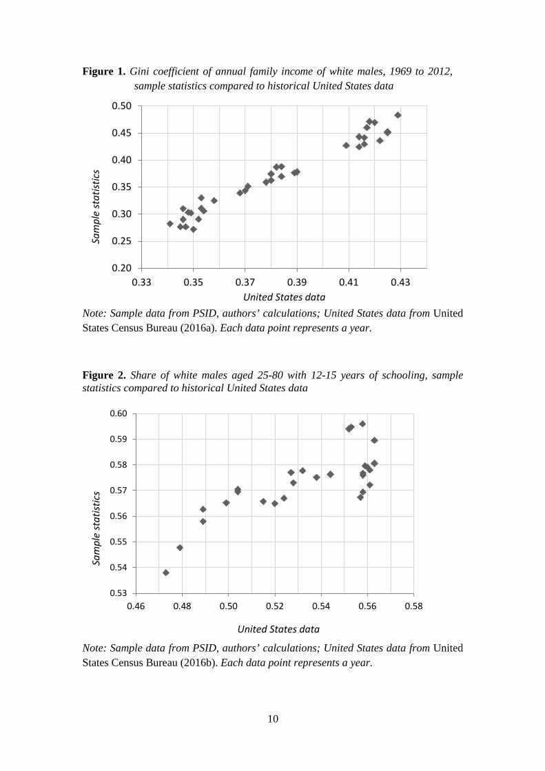
We calculate the sample Gini coefficient for each year from all annual income
observations in that year, from 1969 to 2012, and compared this to the historical time
series of Gini coefficients of the annual income of white households in those years
(United States Census Bureau, 2016a). It yields a very close fit, with a correlation of
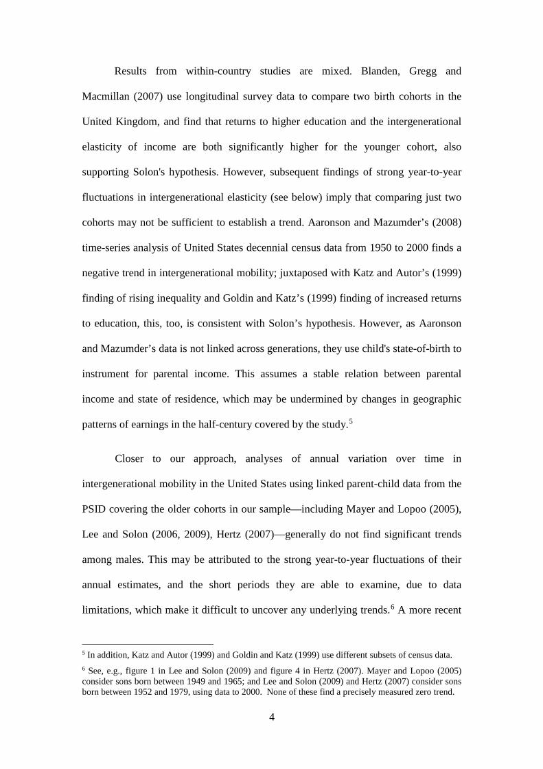
0.98 (Figure 1, and Table A2 in the Appendix). In constructing a time series of
schooling from our sample, we note that individual schooling cannot decline over
time, and so where schooling is reported in a given year and unreported in subsequent
years, we assume that it is unchanged in those years and fill it in. We then compare
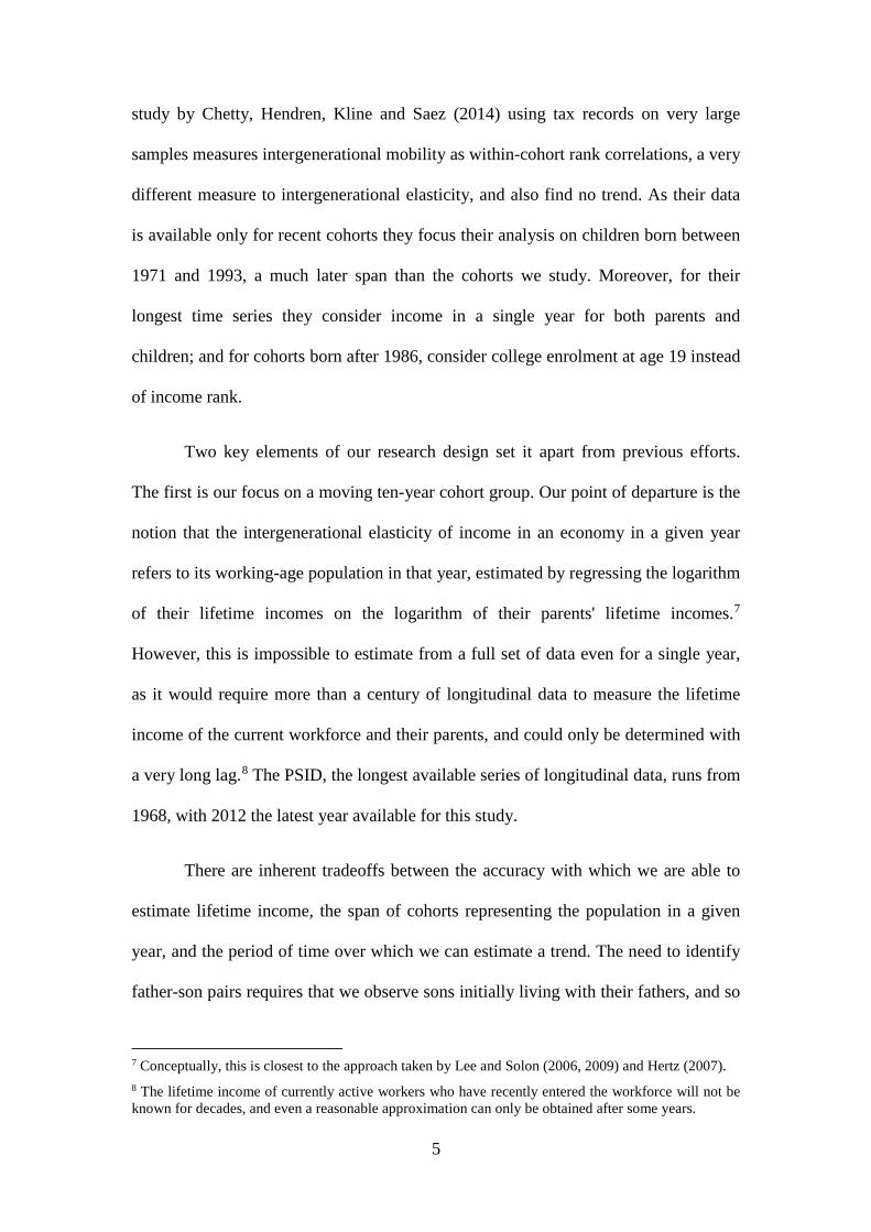
the shares of 25-80 year-olds white men with 12-15 years of schooling in our sample
each year, from 1977 (the year our oldest cohort of sons turns 25) to 2012, to the
historical series (United States Census Bureau, 2016b), and obtain a correlation of
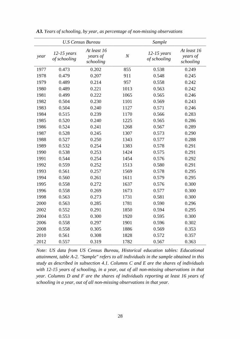
0.78 (Figure 2 and Table A3 in the Appendix).
study may be biased due to nonrandom attrition, and we cannot use the PSID weights for correction. Hertz discussed and implemented a method to generate weights for sub-samples of the PSID with respect to the sample selection criteria in order to overcome the attrition bias.
10
Figure 1. Gini coefficient of annual family income of white males, 1969 to 2012, sample statistics compared to historical United States data
Note: Sample data from PSID, authors’ calculations; United States data from United States Census Bureau (2016a). Each data point represents a year.
Figure 2. Share of white males aged 25-80 with 12-15 years of schooling, sample statistics compared to historical United States data
Note: Sample data from PSID, authors’ calculations; United States data from United States Census Bureau (2016b). Each data point represents a year.
0.20
0.25
0.30
0.35
0.40
0.45
0.50
0.33 0.35 0.37 0.39 0.41 0.43
Sam
ple
stat
istic
s
United States data
0.53
0.54
0.55
0.56
0.57
0.58
0.59
0.60
0.46 0.48 0.50 0.52 0.54 0.56 0.58
Sam
ple
stat
istic
s
United States data
11
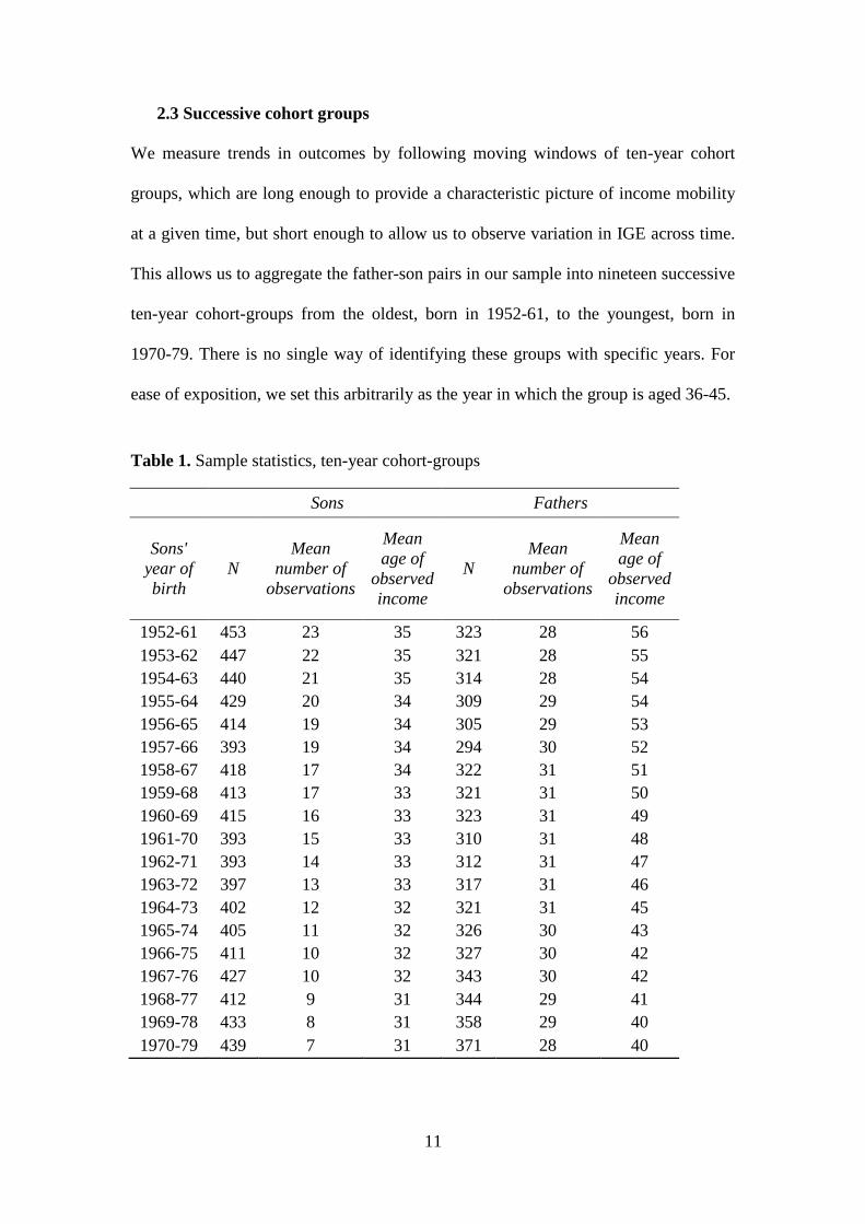
2.3 Successive cohort groups
We measure trends in outcomes by following moving windows of ten-year cohort
groups, which are long enough to provide a characteristic picture of income mobility
at a given time, but short enough to allow us to observe variation in IGE across time.
This allows us to aggregate the father-son pairs in our sample into nineteen successive
ten-year cohort-groups from the oldest, born in 1952-61, to the youngest, born in
1970-79. There is no single way of identifying these groups with specific years. For
ease of exposition, we set this arbitrarily as the year in which the group is aged 36-45.
Table 1. Sample statistics, ten-year cohort-groups
Sons Fathers
Sons' year of birth
N Mean
number of observations
Mean age of
observed income
N Mean
number of observations
Mean age of
observed income
1952-61 453 23 35 323 28 56 1953-62 447 22 35 321 28 55 1954-63 440 21 35 314 28 54 1955-64 429 20 34 309 29 54 1956-65 414 19 34 305 29 53 1957-66 393 19 34 294 30 52 1958-67 418 17 34 322 31 51 1959-68 413 17 33 321 31 50 1960-69 415 16 33 323 31 49 1961-70 393 15 33 310 31 48 1962-71 393 14 33 312 31 47 1963-72 397 13 33 317 31 46 1964-73 402 12 32 321 31 45 1965-74 405 11 32 326 30 43 1966-75 411 10 32 327 30 42 1967-76 427 10 32 343 30 42 1968-77 412 9 31 344 29 41 1969-78 433 8 31 358 29 40 1970-79 439 7 31 371 28 40
12
The size of these cohort-groups ranges between 393 and 453 father-son pairs,
with an average of 416 (descriptive statistics in Table 1). Cohort-groups are similar in
the average number of income observations per father, between 28 and 31, while the
average age at which father’s income is observed drops from 56 for the youngest
cohort-group to 40 for the oldest cohort-group. Given the large number of years of
father’s income data for all groups and our focus on father’s estimated income at age,
these age disparities should not affect our results. The average age at which son’s
labor-income is observed varies in a much narrower range, dropping from 35 to 31,
while the average number of observations per son drops more sharply, from 23 for the
oldest cohort-group to 7 for the youngest cohort-group. Sons’ average years of
education range from 14.04 to 14.38 and are negatively correlated with the share of
sons with 12-15 years of education, with a correlation of -0.92.
3. Empirical method
To characterize the relationship between intergenerational mobility, inequality and
returns to human capital, as they vary over time for our nineteen successive cohort-
groups, we use the two-stage method introduced in Justman and Krush (2013). In the
first stage, we predict individual income at age forty, within each cohort-group, which
serves as our proxy for lifetime income. Then, in the second stage, we use these
proxies for lifetime income to estimate the intergenerational elasticity of lifetime
income, the 90-10 log earnings gap (as our measure of income inequality), and returns
to years of schooling, within each cohort group, producing three time series, and
calculate pairwise correlations. Strong positive correlations support Solon's (2004)
theory with regard to the covariation of these measures over time.
13
3.1 Estimating lifetime income
The first stage of estimating the IGE and other measures relevant to our analysis is to
estimate sons' lifetime earnings and fathers' lifetime income, in the sample extracted
from the PSID. Haider and Solon (2006) show that using income at age forty as a
proxy for lifetime income minimizes attenuation bias, yielding a bias that is not
statistically different from zero. Therefore, we use the predicted labor-income of sons
at the age of forty as a proxy for their lifetime-labor income, and fathers' predicted
family income at the age of forty as a proxy for lifetime family income.
To this purpose we use an expanded version of the Mincer wage equation:
(1) 𝑦𝑦𝑖𝑖𝑖𝑖 = 𝛼𝛼1𝑖𝑖𝐷𝐷𝑖𝑖 + 𝛼𝛼2𝐴𝐴𝐴𝐴𝑒𝑒𝑖𝑖𝑖𝑖 + 𝛼𝛼3𝐴𝐴𝐴𝐴𝑒𝑒𝑖𝑖𝑖𝑖2 + 𝛼𝛼4𝐸𝐸𝐸𝐸𝐸𝐸𝑐𝑐𝑖𝑖 ∙ 𝐴𝐴𝐴𝐴𝑒𝑒𝑖𝑖𝑖𝑖 + 𝛼𝛼5𝐸𝐸𝐸𝐸𝐸𝐸𝑐𝑐𝑖𝑖 ∙ 𝐴𝐴𝐴𝐴𝑒𝑒𝑖𝑖𝑖𝑖2
+ 𝛼𝛼6𝑀𝑀𝑀𝑀𝑀𝑀𝑀𝑀𝑀𝑀𝑀𝑀𝑀𝑀𝑖𝑖𝑖𝑖 ∙ 𝐴𝐴𝐴𝐴𝑒𝑒𝑖𝑖𝑖𝑖 + 𝛼𝛼7𝑀𝑀𝑀𝑀𝑀𝑀𝑀𝑀𝑀𝑀𝑀𝑀𝑀𝑀𝑖𝑖𝑖𝑖 ∙ 𝐴𝐴𝐴𝐴𝑒𝑒𝑖𝑖𝑖𝑖2 + 𝜀𝜀𝑖𝑖𝑖𝑖
where 𝑦𝑦𝑖𝑖𝑖𝑖 is individual's i's labor income or family income in year j. Family income
includes the taxable income of the head of the family and his wife, and transfer
payments. All income data is corrected to 2010 dollars using the Consumer Price
Index; and labor and family income are both bottom- and top-coded at annual levels
of, respectively, $150 and $150,000 in 1967 dollars.14 𝐷𝐷𝑖𝑖 is an individual indicator
variable; 𝐴𝐴𝐴𝐴𝑒𝑒 𝑖𝑖𝑖𝑖 is an individual's age in year j minus 40; 𝐸𝐸𝐸𝐸𝐸𝐸𝑐𝑐𝑖𝑖 represents a set of
indicator variables for 8 years of schooling or less, 8-10 years, 11-12, 13-15, 16 and
17 years or more. Individual education is equal to the highest reported value of years
of schooling in the survey; 𝑀𝑀𝑀𝑀𝑀𝑀𝑀𝑀𝑀𝑀𝑀𝑀𝑀𝑀𝑖𝑖𝑖𝑖 is a set of indicator variables for individual i's
14 Annual earnings below $150 are set equal to $150 and above $150,000 are set equal to $150,000. The reasoning behind this is that our sample sizes are small, and OLS regressions, which we use, are generally sensitive to extreme income values, and all the more so for a log-log specification of income, which is sensitive to the treatment of small values. Chetty et al. (2014), Lee and Solon (2009) and Hertz (2007) trimmed values over $150,000 and below $150 (in 1967 dollars), and Mayer and Lopoo (2005) trimmed the upper and lower 1% observations.
14
marital status at year j: married, never married, widowed, divorced and separated; 𝜀𝜀𝑖𝑖𝑖𝑖
is an i.i.d. error term; 𝛼𝛼1𝑖𝑖,𝛼𝛼2 …𝛼𝛼7 are the regression coefficients. When individual i's
age is forty the variable 𝐴𝐴𝐴𝐴𝑒𝑒 𝑖𝑖𝑖𝑖 takes the value of 0, and the individual's predicted
income is equal to 𝛼𝛼1𝑖𝑖, the coefficient of the individual indicator variable Di.
We predict individual income by cohort-group separately for sons and fathers,
which allows the regression coefficients to change between cohort-groups.15 There are
at most 10 predictions for each individual, a single prediction for sons born in 1952 or
1979 who participate in one cohort-group, and for their fathers. Sons born in 1953 or
1978, and their fathers, participate in 2 cohort groups and have 2 income predictions,
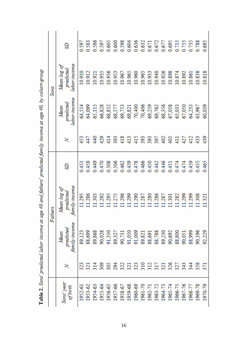
and so on. The mean and standard deviation of predicted lifetime income for fathers
and sons, by cohort-group, are presented in Table 2. Fathers' mean family income and
its standard deviation are stable over time, while sons' mean labor income follows an
inverted U-shaped pattern, and its standard deviation increases. It is not possible to
assess recent trends in mobility in lifetime income without some extrapolation, and
while we limit our attention to sons’ with what we believe is a reasonable basis for
estimating lifetime income, there is an innate difference between these estimates for
younger cohorts of sons still in their thirties, and those obtained for fathers or for
older cohorts in their late forties or fifties. Where the income estimates for older
individuals describe realized lifetime income, those for younger cohorts are an
extrapolation based on past trends that may change over time. This is especially true
for the youngest cohorts, for whom we observe the short-term effects of the 2008
recession, but not its longer term effects.
15 This follows Hertz (2007), Aaronson and Mazumder (2008) and Justman and Krush (2013), all of whom allow the age-earnings profile to change over time.
15
3.2 Estimating intergenerational mobility, inequality and returns to schooling
In the second stage, we estimate measures of intergenerational mobility, inequality
and the return to human capital for each cohort-group.
We measure intergenerational immobility—the extent to which economic
differences between families persist—as the intergenerational elasticity of income,
regressing the logarithm of our estimate of son's lifetime earnings on the logarithm of
our estimate of their parents’ family lifetime income:
(2) 𝑙𝑙𝑙𝑙 𝑦𝑦𝑖𝑖 = 𝛼𝛼 + 𝛽𝛽 𝑙𝑙𝑙𝑙 𝑥𝑥𝑖𝑖 + 𝜀𝜀𝑖𝑖
where 𝑦𝑦𝑖𝑖 is son i's predicted labor-income at age forty; 𝑥𝑥𝑖𝑖 is his father's predicted
family income at age forty; and 𝛽𝛽 is our estimate of the intergenerational elasticity of
income. It is an inverse measure of mobility, measuring persistence of income across
generations—larger values imply slower regression to the mean. Our sensitivity
analysis considers three alternative measures of mobility: the intergenerational
correlation of predicted income at age forty, of its logarithm, and of its rank.
Our measure of income inequality, the 90-10 log wage gap, follows Katz and
Author (1999), with the significant exception that we apply it to our estimate of
lifetime earnings.16 It is the gap between the logarithm of predicted income at age
forty at the 90th and the 10th percentiles of the distribution of sons’ lifetime earnings,
within each ten-year cohort-group. Larger values indicate greater inequality. Our
sensitivity analysis considers two alternative measures of inequality: the coefficient of
variation of the logarithm of sons’ predicted earnings at age forty; and the Gini
coefficient of their predicted earnings at age forty.
16 Katz and Autor consider variation in annual income at a point in time.
16
17
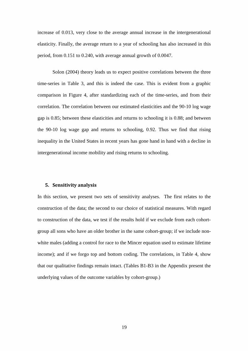
We use average lifetime returns to a year of schooling as our measure of
returns to human capital, which we estimate by regressing the logarithm of sons’
predicted earnings at age forty on years of schooling within each ten-year cohort
group of sons. Our sensitivity analysis considers an alternative measure, the college
premium, following Goldin and Katz (1999).
4. Results
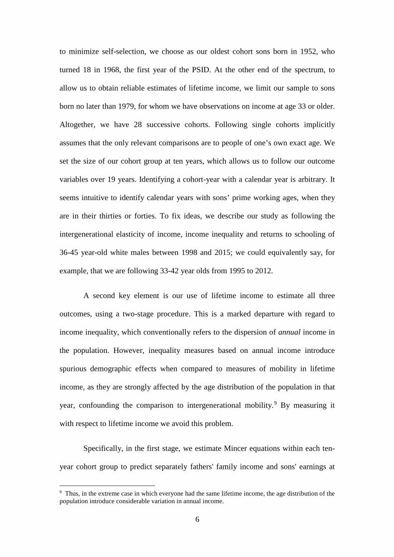
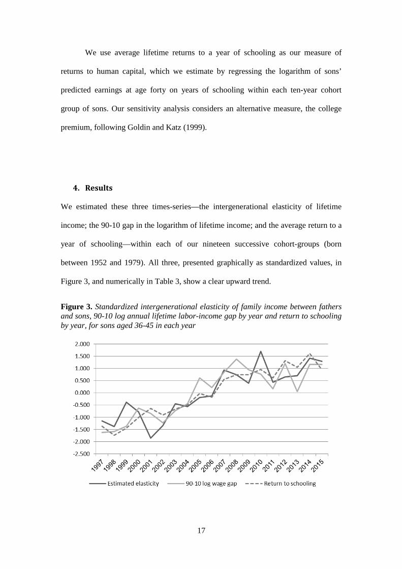
We estimated these three times-series—the intergenerational elasticity of lifetime
income; the 90-10 gap in the logarithm of lifetime income; and the average return to a
year of schooling—within each of our nineteen successive cohort-groups (born
between 1952 and 1979). All three, presented graphically as standardized values, in
Figure 3, and numerically in Table 3, show a clear upward trend.
Figure 3. Standardized intergenerational elasticity of family income between fathers and sons, 90-10 log annual lifetime labor-income gap by year and return to schooling by year, for sons aged 36-45 in each year
18
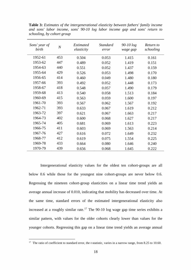
Table 3: Estimates of the intergenerational elasticity between fathers' family income and sons' labor income, sons' 90-10 log labor income gap and sons' return to schooling, by cohort group
Sons' year of birth N Estimated
elasticity Standard
error 90-10 log wage gap
Return to schooling
1952-61 453 0.504 0.053 1.415 0.161 1953-62 447 0.489 0.052 1.419 0.151 1954-63 440 0.551 0.052 1.437 0.159 1955-64 429 0.526 0.053 1.498 0.170 1956-65 414 0.460 0.049 1.480 0.180 1957-66 393 0.492 0.052 1.448 0.173 1958-67 418 0.548 0.057 1.490 0.179 1959-68 413 0.540 0.058 1.513 0.184 1960-69 415 0.563 0.059 1.600 0.197 1961-70 393 0.567 0.062 1.567 0.192 1962-71 393 0.633 0.067 1.619 0.212 1963-72 397 0.621 0.067 1.663 0.217 1964-73 402 0.600 0.068 1.627 0.217 1965-74 405 0.681 0.069 1.613 0.223 1966-75 411 0.603 0.069 1.563 0.214 1967-76 427 0.616 0.072 1.649 0.232 1968-77 412 0.619 0.075 1.554 0.225 1969-78 433 0.664 0.080 1.646 0.240 1970-79 439 0.656 0.068 1.645 0.222
Intergenerational elasticity values for the oldest ten cohort-groups are all
below 0.6 while those for the youngest nine cohort-groups are never below 0.6.
Regressing the nineteen cohort-group elasticities on a linear time trend yields an
average annual increase of 0.010, indicating that mobility has decreased over time. At
the same time, standard errors of the estimated intergenerational elasticity also
increased at a roughly similar rate.17 The 90-10 log wage gap time series exhibits a
similar pattern, with values for the older cohorts clearly lower than values for the
younger cohorts. Regressing this gap on a linear time trend yields an average annual
17 The ratio of coefficient to standard error, the t-statistic, varies in a narrow range, from 8.25 to 10.60.
19
increase of 0.013, very close to the average annual increase in the intergenerational
elasticity. Finally, the average return to a year of schooling has also increased in this
period, from 0.151 to 0.240, with average annual growth of 0.0047.
Solon (2004) theory leads us to expect positive correlations between the three
time-series in Table 3, and this is indeed the case. This is evident from a graphic
comparison in Figure 4, after standardizing each of the time-series, and from their
correlation. The correlation between our estimated elasticities and the 90-10 log wage
gap is 0.85; between these elasticities and returns to schooling it is 0.88; and between
the 90-10 log wage gap and returns to schooling, 0.92. Thus we find that rising
inequality in the United States in recent years has gone hand in hand with a decline in
intergenerational income mobility and rising returns to schooling.
5. Sensitivity analysis
In this section, we present two sets of sensitivity analyses. The first relates to the
construction of the data; the second to our choice of statistical measures. With regard
to construction of the data, we test if the results hold if we exclude from each cohort-
group all sons who have an older brother in the same cohort-group; if we include non-
white males (adding a control for race to the Mincer equation used to estimate lifetime
income); and if we forgo top and bottom coding. The correlations, in Table 4, show
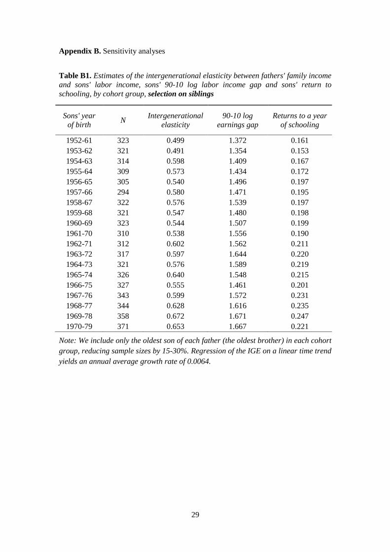
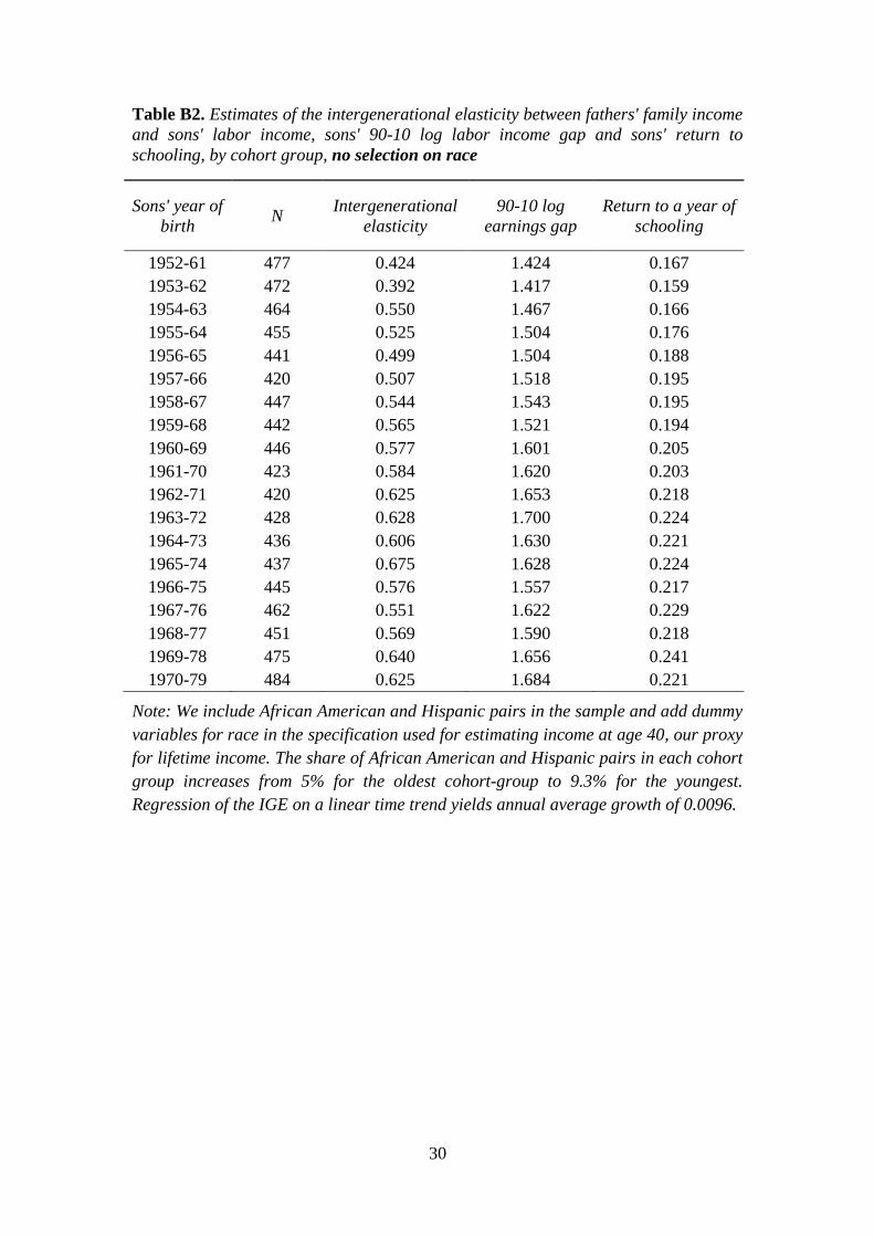
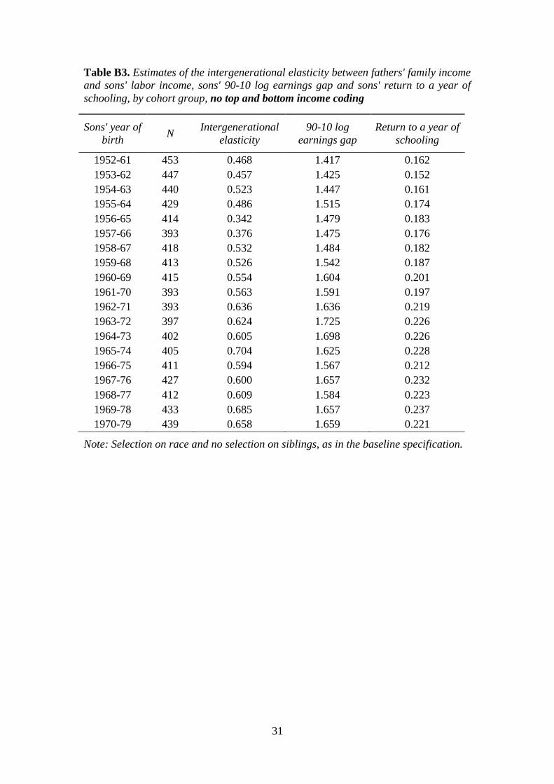
that our qualitative findings remain intact. (Tables B1-B3 in the Appendix present the
underlying values of the outcome variables by cohort-group.)
20
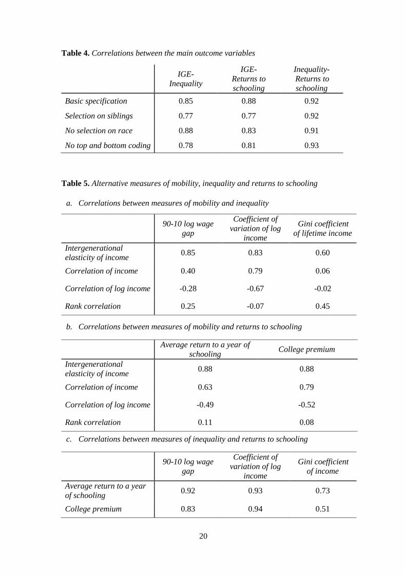
Table 4. Correlations between the main outcome variables
IGE- Inequality
IGE- Returns to schooling
Inequality- Returns to schooling
Basic specification 0.85 0.88 0.92
Selection on siblings 0.77 0.77 0.92
No selection on race 0.88 0.83 0.91
No top and bottom coding 0.78 0.81 0.93
Table 5. Alternative measures of mobility, inequality and returns to schooling
a. Correlations between measures of mobility and inequality
90-10 log wage gap
Coefficient of variation of log
income
Gini coefficient of lifetime income
Intergenerational elasticity of income 0.85 0.83 0.60
Correlation of income 0.40 0.79 0.06
Correlation of log income -0.28 -0.67 -0.02
Rank correlation 0.25 -0.07 0.45
b. Correlations between measures of mobility and returns to schooling
Average return to a year of schooling College premium
Intergenerational elasticity of income 0.88 0.88
Correlation of income 0.63 0.79
Correlation of log income -0.49 -0.52
Rank correlation 0.11 0.08
c. Correlations between measures of inequality and returns to schooling
90-10 log wage gap
Coefficient of variation of log
income
Gini coefficient of income
Average return to a year of schooling 0.92 0.93 0.73
College premium 0.83 0.94 0.51
21
The second set of tests considers alternative measures of intergenerational mobility,
inequality and returns to education, all referring to our basic data specification. We
consider three alternative measures of intergenerational mobility—the Pearson
correlation of lifetime income, the Pearson correlation of the logarithm of lifetime
income, and the Spearman rank correlation of lifetime income (within each cohort-
group); two alternative measures of inequality—the coefficient of variation of the
logarithm of lifetime income and the Gini coefficient of lifetime income; and one
alternative measure of returns to education, the college premium. Their pairwise
correlations are compared in Table 5. (Tables B4-B5 in the Appendix present the
underlying values of the outcome variables by cohort-group.) Panel a presents
correlations between alternative measures of intergenerational mobility and
inequality; panel b presents correlations between alternative measures of
intergenerational mobility and returns to schooling; and panel c presents correlations
between alternative measures of inequality and returns to schooling. Our results are
generally robust to how we measure returns to schooling or inequality but highly
sensitive to how we measure intergenerational mobility.
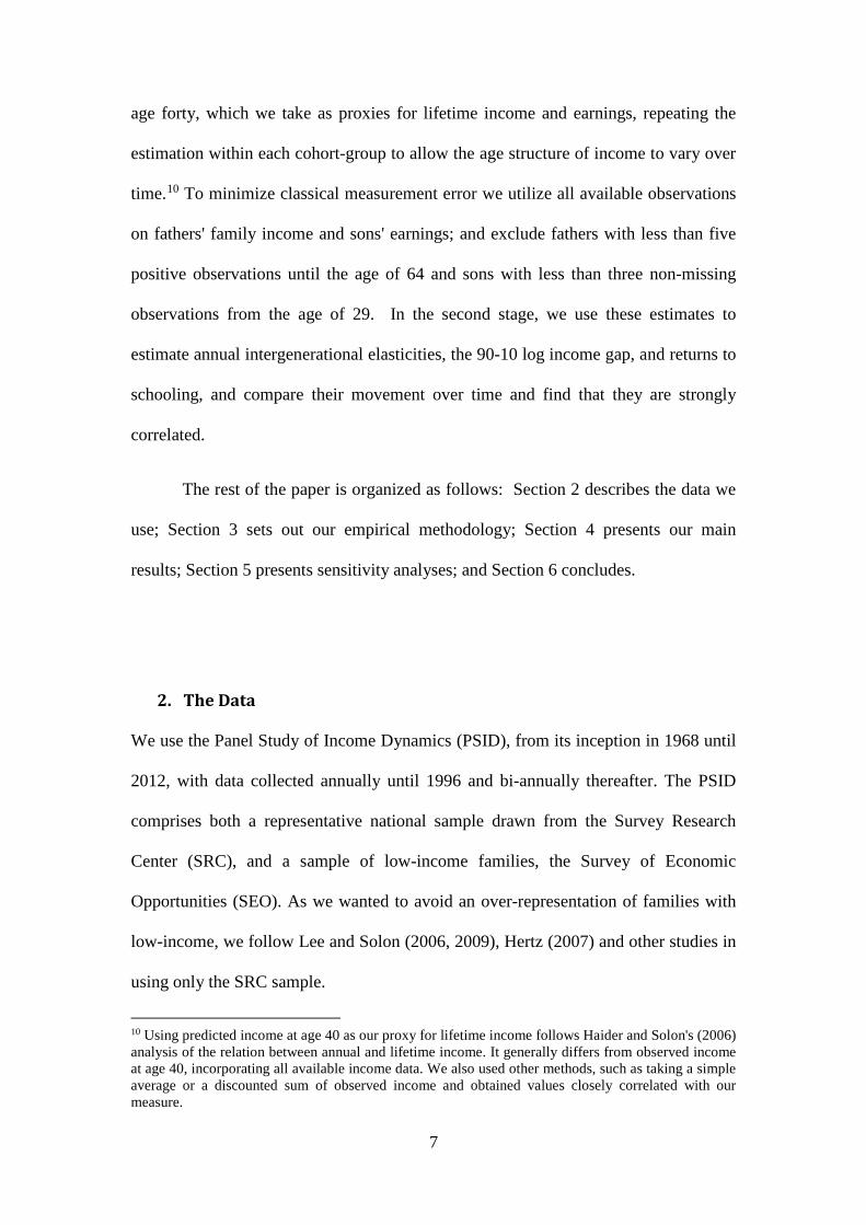
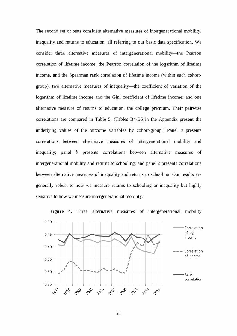
Figure 4. Three alternative measures of intergenerational mobility
0.25
0.30
0.35
0.40
0.45
0.50Correlationof logincome
Correlationof income
Rankcorrelation
22
The three alternative measures of mobility are presented in Figure 4. Each
captures a different dimension of intergenerational mobility (Fields and Ok, 1996).
The correlation of income remains constant for most of the period and then rises
sharply in later years; the correlation of the logarithm of income exhibits a weakly
declining trend; and the rank correlation shows no trend.18 This indicates that the
decline in income mobility reflected in the intergenerational elasticity of income is
closely tied with the rise in inequality, as Solon’s (204) analysis suggests, i.e., with
widening gaps between fixed positions in the rank distribution of earnings rather than
with reduced positional (i.e., rank) mobility. This is also evident in that the estimated
intergenerational elasticity equals the correlation of the logarithm of income
multiplied by the ratio of the standard deviations of sons’ log earnings to fathers’ log
income: in this sense, too, the increase in the dispersion of sons’ income is driving the
rise in the intergenerational elasticity.
6. Conclusions
In this study, we examined the relationships between intergenerational mobility,
inequality and return to human capital over time in the United States, using the PSID
data to 2012. We focus on white father-son pairs for sons born between 1952 and
1979, and limited our attention to father-son pairs in which the son has at least three
non-missing observations on labor income from the age of 29 and the father has at
least five years of non-zero observations of family income until the age of 64. We
exclude non-white pairs because of their under-representation in our PSID sample.
18 Chetty et al. (2014), examining a later period, with some overlap, also find no trend in the intergenerational rank correlation of income.
23
These father-son pairs were aggregated into nineteen successive rolling ten-
year cohort-groups by sons’ year of birth, and we estimated sons' earnings and fathers'
family income at age forty within each of our nineteen cohort-groups, as a proxy for
their lifetime earnings or income. We then used these estimates of lifetime income to
produce three time-series: the intergenerational elasticity of earnings with respect to
family income, as an inverse measure of intergenerational mobility; sons’ 90-10 log
lifetime earnings gap, as a measure of inequality; and sons' average return to a year of
schooling, as a measure of return to human capital.
This approach has several conceptual advantages. It estimates its three time
series from the same set of data; it focuses on lifetime income for all three measures;
and it identifies each year with a ten-year cohort group that is more representative of
that year than a single cohort. Its main weakness is its small, non-random sample size.
Comparing the behavior of our sample 1969 to 2012 with time series for the general
white male population of the United States, we find a correlation of 0.98 for the Gini
coefficient of annual income, and 0.78 for the share of white males aged 36-45 with
12-15 years of schooling.
We then calculated pairwise correlations between these time series, and found
strong, positive co-movement. We found a correlation of 0.85 between the
intergenerational elasticity of income and the 90-10 log earnings gap; 0.88 between
the intergenerational elasticity and returns to human capital; and 0.92 between the 90-
10 log earnings gap and returns to human capital. The results indicate that declining
intergenerational mobility moved in tandem with rising inequality and returns to
human capital in the United States over time, as posited by Solon (2004) and indicated
by some previous suggestive evidence.
24
Our results are generally robust to alternative sampling criteria and to
alternative measures of inequality and returns to human capital but depend strongly on
the choice of measure of intergenerational mobility. They hold weakly if it is
measured as the intergenerational correlation of income but not at all if it is measured
as the intergenerational correlation of the logarithm of income or of income rank. This
highlights the link between rising inequality and reduced mobility.
References
Aaronson, D and B Mazumder, 2008. Intergenerational economic mobility in the United States, 1940 to 2000. Journal of Human Resorces 41(1):139-172.
Becker, G and N Tomes, 1979. An equilibrium theory of the distribution of income and intergenerational mobility. Journal of Political Economy 87(6):1153-1189.
Blanden, J, 2013. Cross‐country rankings in intergenerational mobility: A comparison of approaches from economics and sociology. Journal of Economic Surveys 27(1):38-73.
Blanden, J, P Gregg and L Macmillan, 2007. Accounting for intergenerational income persistence: Noncognitive skills, ability and education. Economic Journal 117(519):C43-C60.
Bratsberg, B, K Røed, O Raaum, R Naylor, M Jäntti, T Eriksson, R Österbacka, 2007. Nonlinearities in intergenerational earnings mobility: Consequences for cross-country comparisons. Economic Journal 117(519): C72-92.
Chadwick, L and G Solon, 2002. Intergenerational income mobility among daughters. American Economic Review 92(1):335-344.
Chetty, R, N Hendren, P Kline, E Saez and N Turner, 2014. Is the United States still a land of opportunity? Recent trends in intergenerational mobility. American Economic Review: Papers and Proceedings 104(5):141–147.
Corak, M, 2013. Income inequality, equality of opportunity, and intergenerational mobility. Journal of Economic Perspectives 27(3):79-102.
Fields, G and E Ok, 1996. The meaning and measurement of income mobility. Journal of Economic Theory 71(2):349-377.
Goldin, C and L Katz, 1999. The returns to skill in the United States across the twentieth century. WP 7126. Cambridge, MA: National Bureau of Economic Research.
25
Haider, S and G Solon, 2006. Life-cycle variation in the association between current and lifetime earnings. American Economic Review 96:1308-1320.
Hertz, T, 2007. Trends in the intergenerational elasticity of family income in the United States. Industrial Relations 46:22-50.
Jerrim, J and L Macmillan, 2015. Income inequality, intergenerational mobility, and the Great Gatsby curve: Is education the key? Social Forces 94:505-533.
Justman, M and A Krush, 2013. Less equal and less mobile: Evidence of a decline in intergenerational income mobility in the United States. WP 43/13, Melbourne Institute of Applied Economic and Social Research, University of Melbourne.
Katz, L and D Autor, 1999. Changes in the wage structure and earnings inequality. In O Ashenfelter and D Card, eds., Handbook of labor economics Vol. 3A, pp. 1463–1555. Amsterdam: Elsevier Science, North-Holland.
Lee, C-I and G Solon, 2006. Trends in intergenerational income mobility. WP 12007. Cambridge, MA: National Bureau of Economic Research.
Lee, C-I and G Solon, 2009. Trends in intergenerational income mobility. Review of Economics and Statistics 91:766-772.
Marks, G N, 2014. Educaton, Social Background and Cognitive Ability: The decline of the social. New York: Routledge.
Mayer, S E and L M Lopoo, 2005. Has the intergenerational transmission of economic status changed? Journal of Human Resources 40:169-185.
Mazumder, B, 2005. Fortunate sons: new estimates of intergenerational mobility in the U.S. using social security earnings data. Review of Economics and Statistics 87(2):235–55.
Solon, G, 2004. A model of intergenerational mobility variation over time and place. In M. Corak, ed., Generational Income Mobility in North America and Europe, pp. 38-47. Cambridge University Press.
United States Census Bureau, 2016a. Historical Income tables: Income Inequality, Table H-4. Retrieved October 2016 from: http://www.census.gov/data/tables/ time-series/demo/income-poverty/historical-income-households.html
United States Census Bureau, 2016b. Historical education tables: Educational attainment, Table A-2. Retrieved October 2016, from: https://www.census. gov/hhes/socdemo/education/data/cps/historical/
26
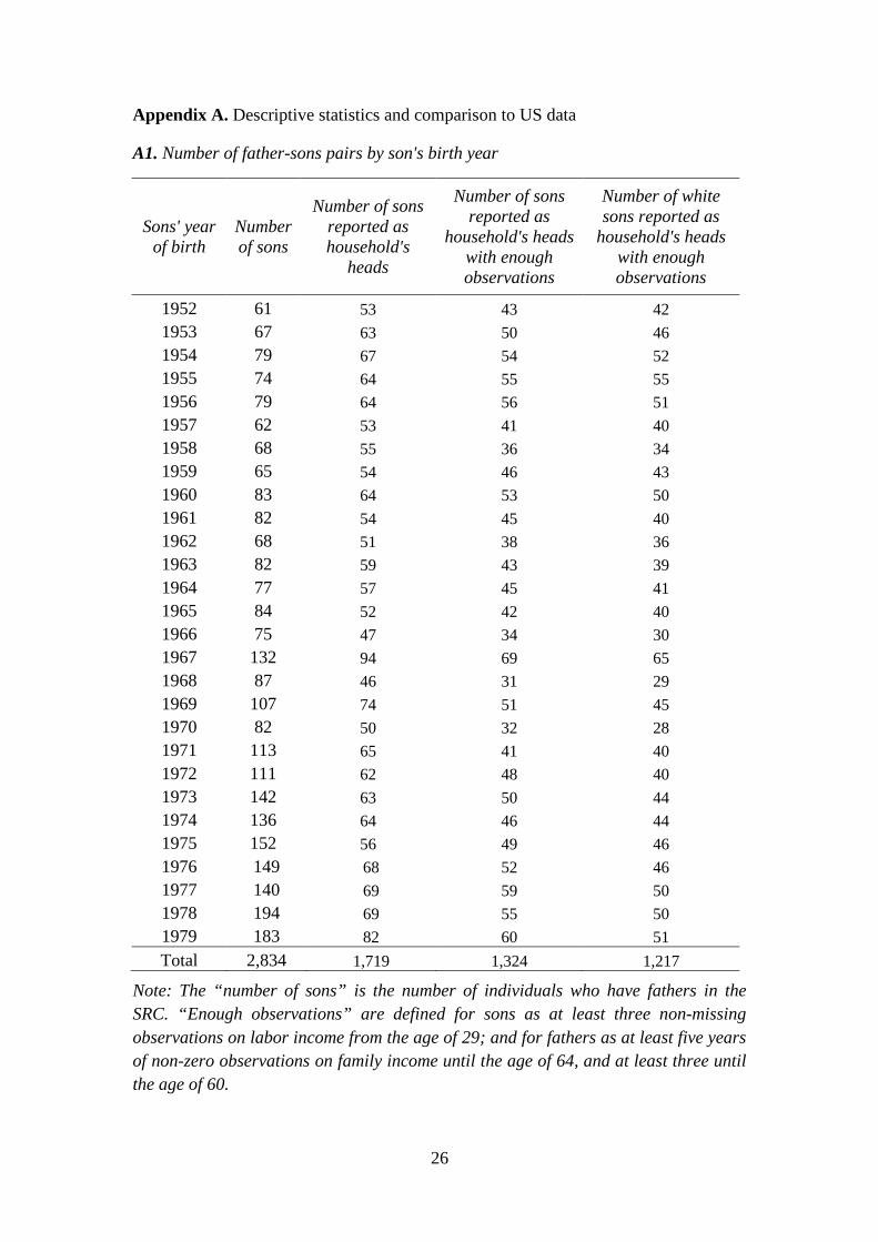
Appendix A. Descriptive statistics and comparison to US data
A1. Number of father-sons pairs by son's birth year
Sons' year of birth
Number of sons
Number of sons reported as household's
heads
Number of sons reported as
household's heads with enough observations
Number of white sons reported as
household's heads with enough observations
1952 61 53 43 42 1953 67 63 50 46 1954 79 67 54 52 1955 74 64 55 55 1956 79 64 56 51 1957 62 53 41 40 1958 68 55 36 34 1959 65 54 46 43 1960 83 64 53 50 1961 82 54 45 40 1962 68 51 38 36 1963 82 59 43 39 1964 77 57 45 41 1965 84 52 42 40 1966 75 47 34 30 1967 132 94 69 65 1968 87 46 31 29 1969 107 74 51 45 1970 82 50 32 28 1971 113 65 41 40 1972 111 62 48 40 1973 142 63 50 44 1974 136 64 46 44 1975 152 56 49 46 1976 149 68 52 46 1977 140 69 59 50 1978 194 69 55 50 1979 183 82 60 51 Total 2,834 1,719 1,324 1,217
Note: The “number of sons” is the number of individuals who have fathers in the SRC. “Enough observations” are defined for sons as at least three non-missing observations on labor income from the age of 29; and for fathers as at least five years of non-zero observations on family income until the age of 64, and at least three until the age of 60.
27
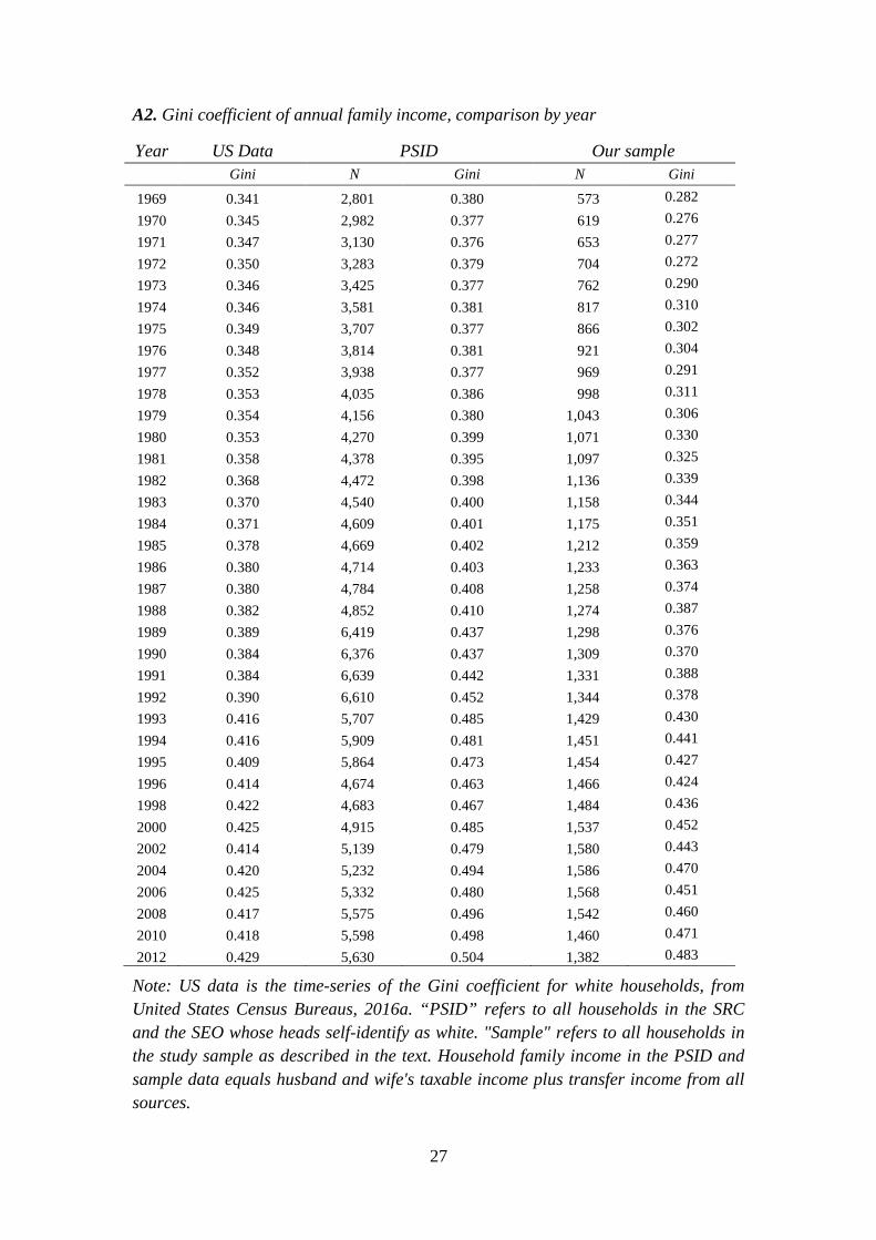
A2. Gini coefficient of annual family income, comparison by year
Year US Data PSID Our sample Gini N Gini N Gini
1969 0.341 2,801 0.380 573 0.282 1970 0.345 2,982 0.377 619 0.276 1971 0.347 3,130 0.376 653 0.277 1972 0.350 3,283 0.379 704 0.272 1973 0.346 3,425 0.377 762 0.290 1974 0.346 3,581 0.381 817 0.310 1975 0.349 3,707 0.377 866 0.302 1976 0.348 3,814 0.381 921 0.304 1977 0.352 3,938 0.377 969 0.291 1978 0.353 4,035 0.386 998 0.311 1979 0.354 4,156 0.380 1,043 0.306 1980 0.353 4,270 0.399 1,071 0.330 1981 0.358 4,378 0.395 1,097 0.325 1982 0.368 4,472 0.398 1,136 0.339 1983 0.370 4,540 0.400 1,158 0.344 1984 0.371 4,609 0.401 1,175 0.351 1985 0.378 4,669 0.402 1,212 0.359 1986 0.380 4,714 0.403 1,233 0.363 1987 0.380 4,784 0.408 1,258 0.374 1988 0.382 4,852 0.410 1,274 0.387 1989 0.389 6,419 0.437 1,298 0.376 1990 0.384 6,376 0.437 1,309 0.370 1991 0.384 6,639 0.442 1,331 0.388 1992 0.390 6,610 0.452 1,344 0.378 1993 0.416 5,707 0.485 1,429 0.430 1994 0.416 5,909 0.481 1,451 0.441 1995 0.409 5,864 0.473 1,454 0.427 1996 0.414 4,674 0.463 1,466 0.424 1998 0.422 4,683 0.467 1,484 0.436 2000 0.425 4,915 0.485 1,537 0.452 2002 0.414 5,139 0.479 1,580 0.443 2004 0.420 5,232 0.494 1,586 0.470 2006 0.425 5,332 0.480 1,568 0.451 2008 0.417 5,575 0.496 1,542 0.460 2010 0.418 5,598 0.498 1,460 0.471 2012 0.429 5,630 0.504 1,382 0.483
Note: US data is the time-series of the Gini coefficient for white households, from United States Census Bureaus, 2016a. “PSID” refers to all households in the SRC and the SEO whose heads self-identify as white. "Sample" refers to all households in the study sample as described in the text. Household family income in the PSID and sample data equals husband and wife's taxable income plus transfer income from all sources.
28
A3. Years of schooling, by year, as percentage of non-missing observations
U.S Census Bureau Sample
year 12-15 years of schooling
At least 16 years of
schooling N 12-15 years
of schooling
At least 16 years of
schooling 1977 0.473 0.202 855 0.538 0.249 1978 0.479 0.207 911 0.548 0.245 1979 0.489 0.214 957 0.558 0.242 1980 0.489 0.221 1013 0.563 0.242 1981 0.499 0.222 1065 0.565 0.246 1982 0.504 0.230 1101 0.569 0.243 1983 0.504 0.240 1127 0.571 0.246 1984 0.515 0.239 1170 0.566 0.283 1985 0.520 0.240 1225 0.565 0.286 1986 0.524 0.241 1268 0.567 0.289 1987 0.528 0.245 1307 0.573 0.290 1988 0.527 0.250 1343 0.577 0.288 1989 0.532 0.254 1383 0.578 0.291 1990 0.538 0.253 1424 0.575 0.291 1991 0.544 0.254 1454 0.576 0.292 1992 0.559 0.252 1513 0.580 0.291 1993 0.561 0.257 1569 0.578 0.295 1994 0.560 0.261 1611 0.579 0.295 1995 0.558 0.272 1637 0.576 0.300 1996 0.558 0.269 1673 0.577 0.300 1998 0.563 0.273 1731 0.581 0.300 2000 0.563 0.285 1781 0.590 0.296 2002 0.552 0.291 1850 0.594 0.295 2004 0.553 0.300 1920 0.595 0.300 2006 0.558 0.297 1901 0.596 0.302 2008 0.558 0.305 1886 0.569 0.353 2010 0.561 0.308 1828 0.572 0.357 2012 0.557 0.319 1782 0.567 0.363
Note: US data from US Census Bureau, Historical education tables: Educational attainment, table A-2. "Sample" refers to all individuals in the sample obtained in this study as described in subsection 4.1. Columns C and E are the shares of individuals with 12-15 years of schooling, in a year, out of all non-missing observations in that year. Columns D and F are the shares of individuals reporting at least 16 years of schooling in a year, out of all non-missing observations in that year.
29
Appendix B. Sensitivity analyses
Table B1. Estimates of the intergenerational elasticity between fathers' family income and sons' labor income, sons' 90-10 log labor income gap and sons' return to schooling, by cohort group, selection on siblings
Sons' year of birth N Intergenerational
elasticity 90-10 log
earnings gap Returns to a year
of schooling
1952-61 323 0.499 1.372 0.161 1953-62 321 0.491 1.354 0.153 1954-63 314 0.598 1.409 0.167 1955-64 309 0.573 1.434 0.172 1956-65 305 0.540 1.496 0.197 1957-66 294 0.580 1.471 0.195 1958-67 322 0.576 1.539 0.197 1959-68 321 0.547 1.480 0.198 1960-69 323 0.544 1.507 0.199 1961-70 310 0.538 1.556 0.190 1962-71 312 0.602 1.562 0.211 1963-72 317 0.597 1.644 0.220 1964-73 321 0.576 1.589 0.219 1965-74 326 0.640 1.548 0.215 1966-75 327 0.555 1.461 0.201 1967-76 343 0.599 1.572 0.231 1968-77 344 0.628 1.616 0.235 1969-78 358 0.672 1.671 0.247 1970-79 371 0.653 1.667 0.221
Note: We include only the oldest son of each father (the oldest brother) in each cohort group, reducing sample sizes by 15-30%. Regression of the IGE on a linear time trend yields an annual average growth rate of 0.0064.
30
Table B2. Estimates of the intergenerational elasticity between fathers' family income and sons' labor income, sons' 90-10 log labor income gap and sons' return to schooling, by cohort group, no selection on race
Sons' year of birth N Intergenerational
elasticity 90-10 log
earnings gap Return to a year of
schooling
1952-61 477 0.424 1.424 0.167 1953-62 472 0.392 1.417 0.159 1954-63 464 0.550 1.467 0.166 1955-64 455 0.525 1.504 0.176 1956-65 441 0.499 1.504 0.188 1957-66 420 0.507 1.518 0.195 1958-67 447 0.544 1.543 0.195 1959-68 442 0.565 1.521 0.194 1960-69 446 0.577 1.601 0.205 1961-70 423 0.584 1.620 0.203 1962-71 420 0.625 1.653 0.218 1963-72 428 0.628 1.700 0.224 1964-73 436 0.606 1.630 0.221 1965-74 437 0.675 1.628 0.224 1966-75 445 0.576 1.557 0.217 1967-76 462 0.551 1.622 0.229 1968-77 451 0.569 1.590 0.218 1969-78 475 0.640 1.656 0.241 1970-79 484 0.625 1.684 0.221
Note: We include African American and Hispanic pairs in the sample and add dummy variables for race in the specification used for estimating income at age 40, our proxy for lifetime income. The share of African American and Hispanic pairs in each cohort group increases from 5% for the oldest cohort-group to 9.3% for the youngest. Regression of the IGE on a linear time trend yields annual average growth of 0.0096.
31
Table B3. Estimates of the intergenerational elasticity between fathers' family income and sons' labor income, sons' 90-10 log earnings gap and sons' return to a year of schooling, by cohort group, no top and bottom income coding
Sons' year of birth N Intergenerational
elasticity 90-10 log
earnings gap Return to a year of
schooling
1952-61 453 0.468 1.417 0.162 1953-62 447 0.457 1.425 0.152 1954-63 440 0.523 1.447 0.161 1955-64 429 0.486 1.515 0.174 1956-65 414 0.342 1.479 0.183 1957-66 393 0.376 1.475 0.176 1958-67 418 0.532 1.484 0.182 1959-68 413 0.526 1.542 0.187 1960-69 415 0.554 1.604 0.201 1961-70 393 0.563 1.591 0.197 1962-71 393 0.636 1.636 0.219 1963-72 397 0.624 1.725 0.226 1964-73 402 0.605 1.698 0.226 1965-74 405 0.704 1.625 0.228 1966-75 411 0.594 1.567 0.212 1967-76 427 0.600 1.657 0.232 1968-77 412 0.609 1.584 0.223 1969-78 433 0.685 1.657 0.237 1970-79 439 0.658 1.659 0.221
Note: Selection on race and no selection on siblings, as in the baseline specification.
32
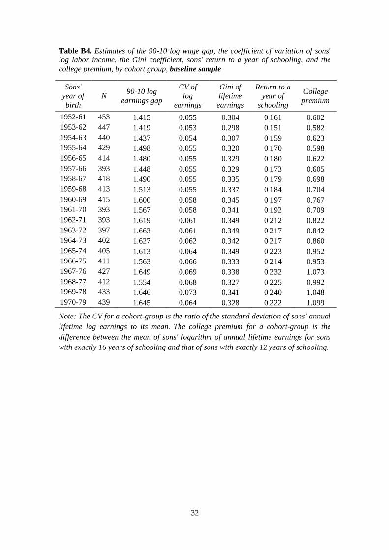
Table B4. Estimates of the 90-10 log wage gap, the coefficient of variation of sons' log labor income, the Gini coefficient, sons' return to a year of schooling, and the college premium, by cohort group, baseline sample
Sons' year of birth
N 90-10 log earnings gap
CV of log
earnings
Gini of lifetime earnings
Return to a year of
schooling
College premium
1952-61 453 1.415 0.055 0.304 0.161 0.602 1953-62 447 1.419 0.053 0.298 0.151 0.582 1954-63 440 1.437 0.054 0.307 0.159 0.623 1955-64 429 1.498 0.055 0.320 0.170 0.598 1956-65 414 1.480 0.055 0.329 0.180 0.622 1957-66 393 1.448 0.055 0.329 0.173 0.605 1958-67 418 1.490 0.055 0.335 0.179 0.698 1959-68 413 1.513 0.055 0.337 0.184 0.704 1960-69 415 1.600 0.058 0.345 0.197 0.767 1961-70 393 1.567 0.058 0.341 0.192 0.709 1962-71 393 1.619 0.061 0.349 0.212 0.822 1963-72 397 1.663 0.061 0.349 0.217 0.842 1964-73 402 1.627 0.062 0.342 0.217 0.860 1965-74 405 1.613 0.064 0.349 0.223 0.952 1966-75 411 1.563 0.066 0.333 0.214 0.953 1967-76 427 1.649 0.069 0.338 0.232 1.073 1968-77 412 1.554 0.068 0.327 0.225 0.992 1969-78 433 1.646 0.073 0.341 0.240 1.048 1970-79 439 1.645 0.064 0.328 0.222 1.099
Note: The CV for a cohort-group is the ratio of the standard deviation of sons' annual lifetime log earnings to its mean. The college premium for a cohort-group is the difference between the mean of sons' logarithm of annual lifetime earnings for sons with exactly 16 years of schooling and that of sons with exactly 12 years of schooling.
33
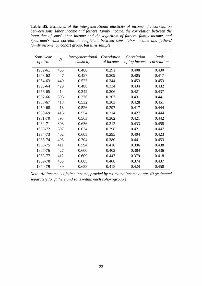
Table B5. Estimates of the intergenerational elasticity of income, the correlation between sons' labor income and fathers' family income, the correlation between the logarithm of sons' labor income and the logarithm of fathers' family income, and Spearman's rank correlation coefficient between sons' labor income and fathers' family income, by cohort group, baseline sample
Sons' year of birth N Intergenerational
elasticity Correlation of income
Correlation of log income
Rank correlation
1952-61 453 0.468 0.291 0.408 0.430 1953-62 447 0.457 0.309 0.405 0.417 1954-63 440 0.523 0.344 0.453 0.453 1955-64 429 0.486 0.334 0.434 0.432 1956-65 414 0.342 0.306 0.421 0.437 1957-66 393 0.376 0.307 0.431 0.441 1958-67 418 0.532 0.303 0.428 0.451 1959-68 413 0.526 0.297 0.417 0.444 1960-69 415 0.554 0.314 0.427 0.444 1961-70 393 0.563 0.302 0.421 0.442 1962-71 393 0.636 0.312 0.433 0.458 1963-72 397 0.624 0.298 0.421 0.447 1964-73 402 0.605 0.295 0.404 0.423 1965-74 405 0.704 0.380 0.441 0.453 1966-75 411 0.594 0.418 0.396 0.438 1967-76 427 0.600 0.402 0.384 0.436 1968-77 412 0.609 0.447 0.379 0.418 1969-78 433 0.685 0.408 0.374 0.437 1970-79 439 0.658 0.418 0.424 0.450
Note: All income is lifetime income, proxied by estimated income at age 40 (estimated separately for fathers and sons within each cohort-group.)