1 3

DOI 10.1007/s00382-016-3027-5Clim Dyn (2016) 47:3301–3317

The interaction between sea ice and salinity‑dominated ocean circulation: implications for halocline stability and rapid changes of sea ice cover

Mari F. Jensen1,2 · Johan Nilsson3 · Kerim H. Nisancioglu1,2

Received: 12 June 2015 / Accepted: 6 February 2016 / Published online: 23 February 2016 © The Author(s) 2016. This article is published with open access at Springerlink.com

not need to increase as much as previously thought to pro-voke abrupt changes in sea ice.

Keywords Sea ice feedbacks · Halocline dynamics · Salinity-dominated ocean circulation · Conceptual model · Dansgaard–Oeschger events

1 Introduction

The mechanism behind Dansgaard–Oeschger (D–O) events, the abrupt climate changes which occurred repeat-edly during the last glacial period, is still debated. One of the hypothesized mechanisms involves a retreating North Atlantic sea ice cover (Broecker 2000; Gildor and Tziperman 2003; Masson-Delmotte et al. 2005; Li et al. 2005). Due to the ice-albedo feedback, the strong insulat-ing effect, and impact on the atmospheric circulation, a changing sea ice cover in the Nordic Seas is a likely agent for the abrupt warming observed on Greenland during D–O events (e.g. Dansgaard et al. 1993; Severinghaus and Brook 1999). Thus, a retreating sea ice cover can explain the tran-sition from cold stadial conditions to warmer, interstadial conditions on Greenland and in the northern North Atlan-tic (Li et al. 2005). In addition, a changing sea ice cover can explain several other features of the abrupt climate events, including precipitation changes (e.g. Peterson et al. 2000; Li et al. 2005, 2010), and changes in dust content (Mayewski et al. 1997). Here, we investigate the interac-tions between sea ice and a salinity-dominated ocean circu-lation in a conceptual model of the Nordic Seas to explore the possible role of sea ice in the abrupt warming associ-ated with D–O events.

Internal instability in the oceanic thermohaline circula-tion, or the Atlantic Meridional Overturning Circulation

Abstract Changes in the sea ice cover of the Nordic Seas have been proposed to play a key role for the dramatic temperature excursions associated with the Dansgaard–Oeschger events during the last glacial. In this study, we develop a simple conceptual model to examine how inter-actions between sea ice and oceanic heat and freshwater transports affect the stability of an upper-ocean halocline in a semi-enclosed basin. The model represents a sea ice covered and salinity stratified Nordic Seas, and consists of a sea ice component and a two-layer ocean. The sea ice thickness depends on the atmospheric energy fluxes as well as the ocean heat flux. We introduce a thickness-dependent sea ice export. Whether sea ice stabilizes or destabilizes against a freshwater perturbation is shown to depend on the representation of the diapycnal flow. In a system where the diapycnal flow increases with density differences, the sea ice acts as a positive feedback on a freshwater perturbation. If the diapycnal flow decreases with density differences, the sea ice acts as a negative feedback. However, both repre-sentations lead to a circulation that breaks down when the freshwater input at the surface is small. As a consequence, we get rapid changes in sea ice. In addition to low fresh-water forcing, increasing deep-ocean temperatures promote instability and the disappearance of sea ice. Generally, the unstable state is reached before the vertical density differ-ence disappears, and the temperature of the deep ocean do

* Mari F. Jensen mari.f.jensen@uib.no

1 Department of Earth Science, University of Bergen, Bergen, Norway

2 Bjerknes Centre for Climate Research, Bergen, Norway3 Department of Meteorology, Stockholm University,

Stockholm, Sweden

3302 M. F. Jensen et al.

1 3

(AMOC) has also been suggested as a mechanism for rapid climate change (Broecker et al. 1990; Tziperman 1997; Marotzke 2000; Ganopolski and Rahmstorf 2001). Broe-cker et al. (1990) first suggested internal oscillations in the volume transport of the AMOC as a mechanism for D–O events. The idea is that a strong circulation transports more heat from the South Atlantic to the North Atlantic, thereby warming the atmosphere at high latitudes. A weak, or an off state of the AMOC could lead to less heat import to the North Atlantic causing cold stadial conditions. Several modeling studies have simulated an AMOC with a strong and a weak state (e.g. Stocker and Wright 1991; Fanning and Weaver 1997; Manabe and Stouffer 1995; Stouffer et al. 2006). However, paleoclimatic reconstructions have shown active formation of North Atlantic Deep Water also during stadials (Yu et al. 1996). Latitudinal shifts in the North Atlantic Deep Water formation site is also hypothesized to account for the D–O events (Ganopolski and Rahmstorf 2001; Arzel et al. 2010; Colin de Verdiere and Raa 2010; Sevellec and Fedorov 2015). Freshwater forcing has typically been the agent to force the different states of the circulation, and the duration of the cold and the warm states generally depend on the duration of the freshwater forcing (Ganopolski and Rahmstorf 2002). On the other hand, Marotzke (1989), Winton (1993) and Win-ton and Sarachik (1993) found self-sustaining oscillations with strong and weak overturning due to increasing deep-ocean temperatures. Their idea is that freshwater input at the poles causes a strong, vertical salinity gradient (halo-cline) which suppresses deep-water formation. The stabil-ity of the high latitude halocline breaks down as diffusion from the south heats the deep ocean. Deep-water formation becomes active again, and warm, light water is transported to the high latitudes which then again stabilizes the water column. These deep-decoupling oscillations bear resem-blances to the D–O stadial and interstadials (Timmermann et al. 2003). Seen in isolation, a changing AMOC gives a temperature response on Greenland which is too slow and too small compared to the observations. However, the addi-tion of a responsive sea ice cover in the Nordic Seas would enhance the temperature response to small internal oscilla-tions in the ocean.

Paleoclimatic reconstructions support a warming of the subsurface Nordic seas during cold stadial conditions (Dok-ken and Jansen 1999; Rasmussen and Thomsen 2004; Dok-ken et al. 2013). In particular, it has been proposed that the warming of the subsurface ocean during cold stadial condi-tions could explain the rapid retreat of sea ice in the Nordic Seas at the start of each interstadial (Dokken et al. 2013). From a marine sediment core from the Faeroe-Shetland channel, Dokken et al. (2013) showed systematic changes in the hydrography of the Nordic Seas during cold stadi-als and warm interstadials. During stadial conditions, the

hydrography was similar to the Arctic Ocean today, with a cold, fresh surface layer above a warmer Atlantic layer. A sharp halocline marks the transition between the two dif-ferent water masses, protecting the surface layer from the heat below. The authors proposed that the vertical density gradient and the halocline would gradually weaken due to a slow warming of the deep ocean. Eventually, as the verti-cal density difference disappeared, the stability of the water column would break down. When the halocline is gone, the Atlantic layer would mix to the surface, melting the sea ice cover. This scenario is dependent on a mechanism that gradually increases the temperature of the Atlantic layer.

A different scenario involves slow changes in the fresh-water supply to the ocean. By using an analytical two-layer ocean model, Nilsson and Walin (2010) showed that the salinity-dominated (estuarine) circulation and halocline can break down even before the vertical density gradient van-ishes. If this is also true for ice-covered conditions, which can entail additional feedbacks, the convective overturn-ing proposed by Dokken et al. (2013) could occur at low freshwater inputs, even before the vertical density gradient disappears. This would be highly relevant for cold, dry gla-cial climates. An interesting question is at what point the halocline disappears given a constant temperature below the halocline.

However, the properties of thermohaline circulations are dependent on the relation between flow strength and density differences. In thermohaline models which include vertical mixing, the flow strength is sensitive to how the vertical velocity is represented (Lyle 1997; Huang 1999; Nilsson and Walin 2001). Assuming a fixed external energy supply to the small scale mixing, Nilsson and Walin (2010) repre-sented the vertical velocity with a stratification-dependent vertical diffusivity. The result is a diapycnal velocity which decreases with increasing stratification and an ocean cir-culation which acts in the same way. If instead, diapycnal velocity is represented with a constant diffusivity, the ocean circulation increases with increasing stratification (e.g. Bryan 1986; Zhang et al. 1999; Nilsson and Walin 2001). As the classical box model by Stommel (1961) involves a flow which speeds up with increasing density difference, the latter representation bears resemblances to the typical Stommel model.

Thus, the stability of the salinity-dominated circulation depends on the assumed properties of the diapycnal mix-ing. In the conceptual model by Nilsson and Walin (2010) the authors found that there is a minimum freshwater input below which the halocline solution no longer exists. In models where the flow strength increases with density dif-ferences, there exists a solution for all freshwater forcing for the salinity-dominated circulation (Zhang et al. 1999; Longworth et al. 2005). If this is the case, other factors, such as increasing subsurface temperatures, are needed to

3303The interaction between sea ice and salinity-dominated ocean circulation

1 3

initiate convective overturning. However, Longworth et al. (2005) and Guan and Huang (2008) showed that the pres-ence of wind-driven, horizontal salt transport destabilizes the thermohaline circulation, and removes the equilibria at weak freshwater supplies. Therefore, additional factors may have the potential to introduce convective overturning due to low freshwater forcing in models with a constant dif-fusivity as well.

As the proposed mechanism by Dokken et al. (2013) involves a sea ice covered Nordic Seas, we add the sea ice model from Thorndike (1992) to the simple two-layer ocean model of Nilsson and Walin (2010). The aim of the study is to investigate how the presence of sea ice affects the dynamics and stability of the salinity-dominated circu-lation as the climatic conditions are varied. As the detailed features of the diapycnal mixing are not well known, we will in this study examine the two different vertical mix-ing representations discussed above. The experiments are divided into an “energy-constrained model”, where we retain the diapycnal velocity from Nilsson and Walin (2010), and a “constant-diffusivity model” where the diapycnal velocity is parametrized with a constant diffusiv-ity. The vertical mixing is expected to change with a chang-ing sea ice cover and climate. Therefore, even though the first case is more physically consistent, it is useful to study different representations of the vertical mixing.

Interactions between sea ice and thermally-dominated thermohaline circulation have been studied in conceptual models by for instance Yang and Neelin (1993, 1997) and Jayne and Marotzke (1999). Using a Stommel-type box model coupled to an energy-balance representation of the atmosphere, Jayne and Marotzke (1999) found that sea ice related feedbacks destabilized the thermally-dominated mode of the thermohaline circulation. In their model, feed-backs between sea ice, meridional temperature gradients and atmospheric moisture transport were of key impor-tance, whereas brine rejection associated with sea ice for-mation played a more central role in the box model of Yang and Neelin (1993). However, less attention has been paid to how sea ice feedbacks affect a salinity-dominated ther-mohaline circulation. Stigebrandt (1981) developed a pro-cess-oriented two-layer model of the Arctic Ocean, which incorporates inflows and outflows, air-sea heat exchange, and sea ice dynamics. Interestingly, Stigebrandt found that the sea ice cover in the model vanished abruptly when the freshwater supply to the Arctic Ocean was reduced below some threshold value. In fact, Nilsson and Walin (2010) essentially used the same geostrophic flow representation as Stigebrandt (1981). However, Stigebrandt’s model con-tains additional complexities which makes it difficult to examine the sea ice related feedbacks in more detail.

In this study, we develop a conceptual model that is simple enough to admit analytical analyses of the key

feedbacks. First, the two-layer ocean model by Nils-son and Walin (2010) and the simplified sea ice model from Thorndike (1992) will be presented in Sect. 2. We review the response of the model to freshwater forcing in the absence of sea ice in Sect. 3. Then, the response of the model to freshwater forcing in the presence of sea ice is presented in Sect. 4. We compare the stabilizing effect of sea ice in the energy-constrained model with the constant-diffusivity model in Sect. 4.2. In Sect. 5, we investigate the effect of increasing deep-ocean tempera-tures on the stability of the system. In Sect. 6, we dis-cuss the impact of the results on the Dokken et al. (2013) hypothesis.

2 Model formulation

Here we will show how the conceptual two-layer ocean model from Nilsson and Walin (2010) can be coupled to the simplified sea ice model from Thorndike (1992). The two model components are presented below, and the cou-pled ocean–ice system can be seen in Fig. 1. Variables that are not defined in the text can be found in Table 1. The sim-plified ocean and ice models used here are well established and used in numerous studies. The novelty of this study is to examine the physics that results from their coupling. Useful background information on the physical motivation and derivation of two-layer ocean models can be found in e.g. Gnanadesikan (1999), Nilsson and Walin (2001) and Johnson et al. (2007). Bitz and Roe (2004) provide a con-cise derivation of the sea ice model from Thorndike (1992).

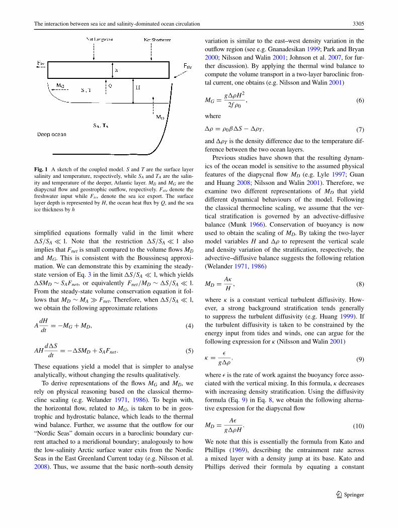
The ocean model consists of a cold, light surface layer, and a warmer, homogeneous deeper layer with the same hydrography as the open ocean. The circulation is that of a salinity-dominated regime, in the sense that supply of freshwater at the surface establishes a stable stratification. The topography is that of a semi-enclosed basin (Fig. 1). The basin receives freshwater from river run-off, precipi-tation, and ice-import, together denoted as Friv. The ocean flow consists of the diapycnal flow MD, and the horizontal geostrophic outflow MG. The diapycnal flow increases the depth of the light surface layer H, while MG thins the sur-face layer.

The subsequent derivations follow Nilsson and Walin (2010). By applying a time-dependent version of the Knud-sen’s relations (Knudsen 1900), the conservation of volume and salinity can be written as

(1)AdH

dt= MD −MG + Fnet ,

(2)AdHS

dt= SAMD − SMG,

3304 M. F. Jensen et al.

1 3

where S is the salinity of the surface layer, SA is the salinity of the Atlantic layer, Fnet = Friv − Fice is the net freshwa-ter input to the surface, Fice is the sea ice export, and A is the area of the Nordic Seas. Note that in steady-state, the above equations become the classical Knudsen’s relations.

By combining Eqs. 1 and 2, we get

(3)AHd�S

dt= −�SMD + (SA −�S)Fnet ,

where �S = SA − S, and SA is a constant. This equation can be simplified further: In the open ocean, away from coastal regions, one typically finds that SA ∼ 35 and �S ∼ 3. Therefore, �S/SA is significantly smaller than unity. This is widely used in oceanography to derive the Boussinesq approximation equations (Vallis 2006) where the surface freshwater flux is substituted by a virtual salt flux bound-ary condition and the freshwater flux is neglected in the volume conservation equation. We exploit this and derive

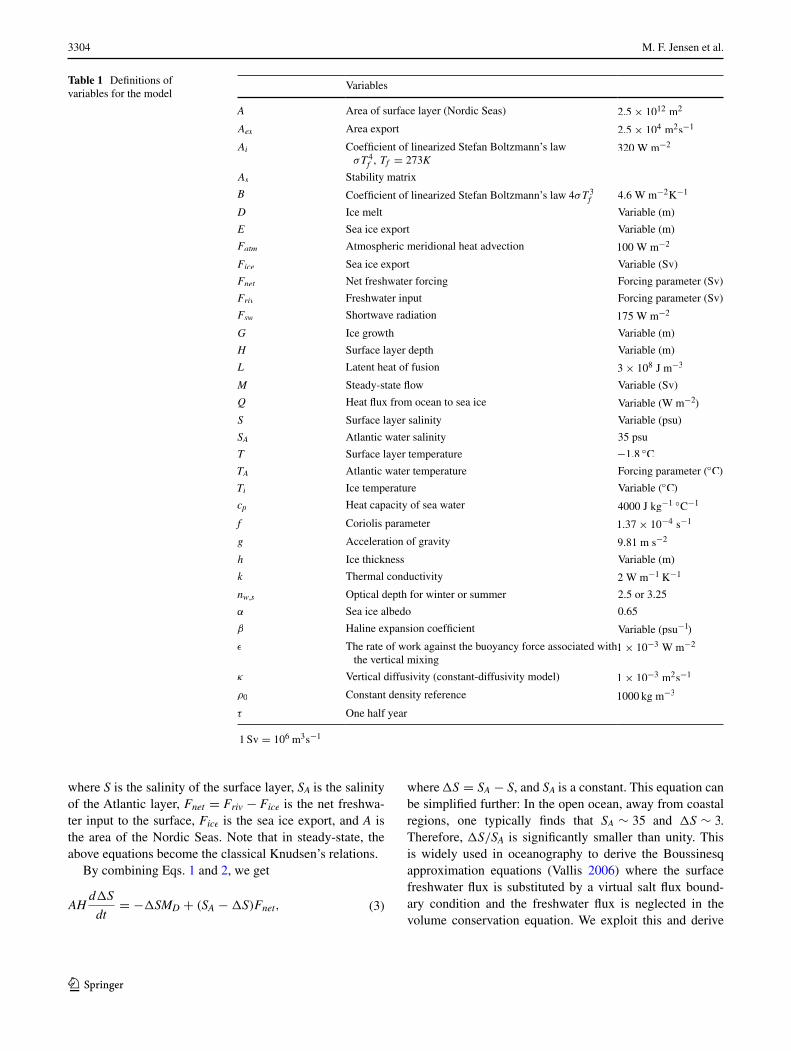
Table 1 Definitions of variables for the model

1 Sv = 106 m3s−1

Variables

A Area of surface layer (Nordic Seas) 2.5× 1012 m2

Aex Area export 2.5× 104 m2s−1

Ai Coefficient of linearized Stefan Boltzmann’s law σT4

f , Tf = 273K320 W m−2

As Stability matrix

B Coefficient of linearized Stefan Boltzmann’s law 4σT3f 4.6 W m−2K−1

D Ice melt Variable (m)

E Sea ice export Variable (m)

Fatm Atmospheric meridional heat advection 100 W m−2

Fice Sea ice export Variable (Sv)

Fnet Net freshwater forcing Forcing parameter (Sv)

Friv Freshwater input Forcing parameter (Sv)

Fsw Shortwave radiation 175 W m−2

G Ice growth Variable (m)

H Surface layer depth Variable (m)

L Latent heat of fusion 3× 108 J m−3

M Steady-state flow Variable (Sv)

Q Heat flux from ocean to sea ice Variable (Wm−2)

S Surface layer salinity Variable (psu)

SA Atlantic water salinity 35 psu

T Surface layer temperature −1.8 ◦C

TA Atlantic water temperature Forcing parameter (◦C)

Ti Ice temperature Variable (◦C)

cp Heat capacity of sea water 4000 J kg−1 ◦C−1

f Coriolis parameter 1.37× 10−4 s−1

g Acceleration of gravity 9.81 m s−2

h Ice thickness Variable (m)

k Thermal conductivity 2 W m−1 K−1

nw,s Optical depth for winter or summer 2.5 or 3.25

α Sea ice albedo 0.65

β Haline expansion coefficient Variable (psu−1)

ǫ The rate of work against the buoyancy force associated with the vertical mixing

1× 10−3 W m−2

κ Vertical diffusivity (constant-diffusivity model) 1× 10−3 m2s−1

ρ0 Constant density reference 1000 kg m−3

τ One half year

3305The interaction between sea ice and salinity-dominated ocean circulation

1 3

simplified equations formally valid in the limit where �S/SA ≪ 1. Note that the restriction �S/SA ≪ 1 also implies that Fnet is small compared to the volume flows MD and MG. This is consistent with the Boussinesq approxi-mation. We can demonstrate this by examining the steady-state version of Eq. 3 in the limit �S/SA ≪ 1, which yields �SMD ∼ SAFnet, or equivalently Fnet/MD ∼ �S/SA ≪ 1. From the steady-state volume conservation equation it fol-lows that MD ∼ MA ≫ Fnet. Therefore, when �S/SA ≪ 1, we obtain the following approximate relations

These equations yield a model that is simpler to analyse analytically, without changing the results qualitatively.

To derive representations of the flows MG and MD, we rely on physical reasoning based on the classical thermo-cline scaling (e.g. Welander 1971, 1986). To begin with, the horizontal flow, related to MG, is taken to be in geos-trophic and hydrostatic balance, which leads to the thermal wind balance. Further, we assume that the outflow for our “Nordic Seas” domain occurs in a baroclinic boundary cur-rent attached to a meridional boundary; analogously to how the low-salinity Arctic surface water exits from the Nordic Seas in the East Greenland Current today (e.g. Nilsson et al. 2008). Thus, we assume that the basic north–south density

(4)AdH

dt= −MG +MD,

(5)AHd�S

dt= −�SMD + SAFnet .

variation is similar to the east–west density variation in the outflow region (see e.g. Gnanadesikan 1999; Park and Bryan 2000; Nilsson and Walin 2001; Johnson et al. 2007, for fur-ther discussion). By applying the thermal wind balance to compute the volume transport in a two-layer baroclinic fron-tal current, one obtains (e.g. Nilsson and Walin 2001)

where

and �ρT is the density difference due to the temperature dif-ference between the two ocean layers.

Previous studies have shown that the resulting dynam-ics of the ocean model is sensitive to the assumed physical features of the diapycnal flow MD (e.g. Lyle 1997; Guan and Huang 2008; Nilsson and Walin 2001). Therefore, we examine two different representations of MD that yield different dynamical behaviours of the model. Following the classical thermocline scaling, we assume that the ver-tical stratification is governed by an advective-diffusive balance (Munk 1966). Conservation of buoyancy is now used to obtain the scaling of MD. By taking the two-layer model variables H and �ρ to represent the vertical scale and density variation of the stratification, respectively, the advective–diffusive balance suggests the following relation (Welander 1971, 1986)

where κ is a constant vertical turbulent diffusivity. How-ever, a strong background stratification tends generally to suppress the turbulent diffusivity (e.g. Huang 1999). If the turbulent diffusivity is taken to be constrained by the energy input from tides and winds, one can argue for the following expression for κ (Nilsson and Walin 2001)

where ǫ is the rate of work against the buoyancy force asso-ciated with the vertical mixing. In this formula, κ decreases with increasing density stratification. Using the diffusivity formula (Eq. 9) in Eq. 8, we obtain the following alterna-tive expression for the diapycnal flow

We note that this is essentially the formula from Kato and Phillips (1969), describing the entrainment rate across a mixed layer with a density jump at its base. Kato and Phillips derived their formula by equating a constant

(6)MG =g�ρH2

2f ρ0,

(7)�ρ = ρ0β�S −�ρT ,

(8)MD =Aκ

H,

(9)κ =ǫ

g�ρ,

(10)MD =Aǫ

g�ρH.

Fig. 1 A sketch of the coupled model. S and T are the surface layer salinity and temperature, respectively, while SA and TA are the salin-ity and temperature of the deeper, Atlantic layer. MD and MG are the diapycnal flow and geostrophic outflow, respectively. Friv denote the freshwater input while Fice denote the sea ice export. The surface layer depth is represented by H, the ocean heat flux by Q, and the sea ice thickness by h

3306 M. F. Jensen et al.

1 3

mechanical energy input with the rate of increase in poten-tial energy caused by the entrainment.

We are interested in the steady-state solutions where M = MD = MG and �SM = SAFnet . We get the steady-state flow and surface layer depth by combining Eq. 6 with Eqs. 8 or 10. For the energy-constrained model, we get;

For the constant-diffusivity model;

2.1 Sea ice model

For the sea ice component, we follow Bitz and Roe (2004) and Thorndike (1992) which estimated equilibrium sea ice thickness h by assuming a quasi-steady balance between sea ice growth G and decay D. The sea ice thickness is esti-mated with only the main essential elements included; the net atmospheric flux incident at the top of the ice, and the heat flux Q from the ocean at the base of the ice. Making use of steady-state heat conduction through sea ice, and an atmosphere which is in thermal radiative equilibrium with the sea ice, we calculate G and D following Bitz and Roe (2004);

where the temperature of the ice Ti is given by

Fatm is the atmospheric meridional heat advection, Fsw is the shortwave insolation, Ai and B are the coefficients of the linearized Stefan Boltzmann’s law, Q is the heat flux from the ocean to the ice, α is the sea ice albedo, τ is one half year, L is the latent heat of fusion, k is the thermal con-ductivity, while nw and ns are the optical depths for winter and summer, respectively.

(11)M =

(

A2ǫ2

g2ρ0f�ρ

)1/3

,

(12)H =

(

Aǫ2ρ0f

g2�ρ2

)1/3

.

(13)M =

(

A2κ2g�ρ

2f ρ0

)1/3

,

(14)H =

(

Aκ2ρ0f

g�ρ

)1/3

.

(15)G(h) =τ

L

[

Ai + BTi(h)

nw−

Fatm

2− Q

]

,

(16)D =τ

L

[

−Ai

ns+

Fatm

2+ Q+ (1− α)Fsw

]

,

(17)Ti(h) =

(

nwh

knw + Bh

)(

−Ai

nw+

Fatm

2

)

.

During summer, Ti = 0 ◦C is assumed, while Fsw = 0 during winter. Fsw is defined as the annual input of short-wave radiation, distributed over the melting season. The growth and melting seasons are each estimated as half of the year.

Decay melt is independent of h, while ∂G/∂h < 0. Thin ice grows faster than thick ice, and as a consequence thick ice is more sensitive to changes in the forcing (Bitz and Roe 2004). Bitz and Roe (2004) showed that the change in thickness increases approximately quadratically with sea ice thickness as thicker ice needs to thin more to establish a new equilibrium.

In this study, we keep the atmospheric and solar energy fluxes constant; see Bitz and Roe (2004) and Stranne and Björk (2012) for the effect of variations in Fsw and Fatm, respectively. Therefore, variations of the steady-state sea ice thickness are controlled by the ocean heat flux, which is a function of the steady-state flow in the ocean;

where �T = TA − T , TA is the Atlantic layer temperature, and T is the temperature of the surface layer. A positive heat flux is directed upward into the ice.

Following Stranne and Björk (2012), we include a thick-ness dependent ice export E in the sea ice model,

where Aex is the areal export. As we study changes in the sea ice thickness on time scales longer than seasonal, we can write;

The equilibrium sea ice thickness can be found by solv-ing for G(h)− D = E(h). Hence, Eqs. 15–17 and 19 can be combined to one equation which can be solved for the unknown h.

When the ocean-model is coupled to the sea ice-model, the ice-export transports freshwater out of the system. Therefore,

where1

(18)Q =cpρ0M�T

A,

(19)E =2τAexh

A,

(20)2τdh

dt= G− D− E.

(21)Fnet = Friv − Fice,

1 For simplicity, the salt content of the sea ice is ignored in the fresh-water budget. This could be accounted for by multiplying Fice with (SA − Sice)/SA, where Sice is the sea ice salinity.

(22)Fice =(G− D)A

2τ.

3307The interaction between sea ice and salinity-dominated ocean circulation

1 3

3 Model response to freshwater in absence of sea ice

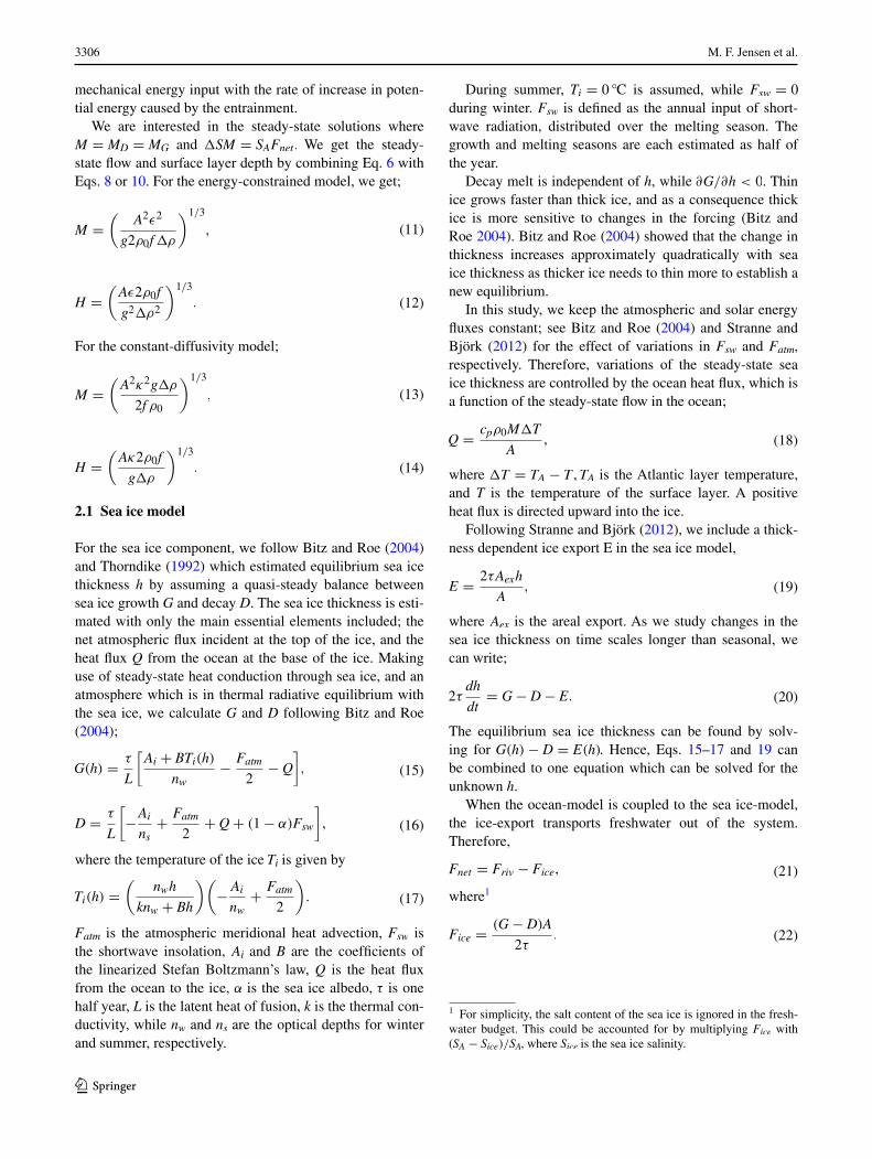
In this section, we study the features of the model in the absence of sea ice. When the diapycnal flow decreases with increasing stratification, the steady-state flow decreases with increasing density differences (Eq. 11). As freshwa-ter inputs at the surface increase the density difference, the flow decreases with freshwater input in the energy-constrained case (Fig. 2c). The surface layer depth also decreases with freshwater forcing (Fig. 2b). Thus, in the limit of small freshwater input, the low salinity surface layer becomes very deep, implying that the upper limit of the warmer Atlantic water layer is displaced to greater depths; a feature which may have relevance for the glacial Arctic Ocean stratification (Jakobsson et al. 2010; Cronin et al. 2012).

Nilsson and Walin (2010) showed that the salinity-domi-nated circulation does not have a solution below a threshold value of Friv. The steady-state solution becomes unstable at small salinity contrasts (Fig. 2, stippled lines). To illustrate the underlying physics, we consider the feedbacks acting on a positive salinity perturbation, which decreases the vertical density difference. As we will show in Sect. 4.2, the mean

flow always stabilizes, advecting away perturbations. How-ever, the reduced vertical density difference is associated with a positive perturbation in the diapycnal flow (Eq. 10), which increases the salt transport to the upper layer. This further reduces the vertical salinity and density contrast, resulting in a positive feedback. For sufficiently small salin-ity contrasts, the positive feedback becomes larger than the negative feedback, and the system becomes unstable. In the more detailed stability analysis presented in the next section, it is shown that the flow becomes unstable when ρoβ�S < 1.5�ρT. As this limit is approached, the halocline solution breaks down and the surface layer is suggested to extend toward great depths (Fig. 2b). Additional physics need to be incorporated into the model to study this regime.

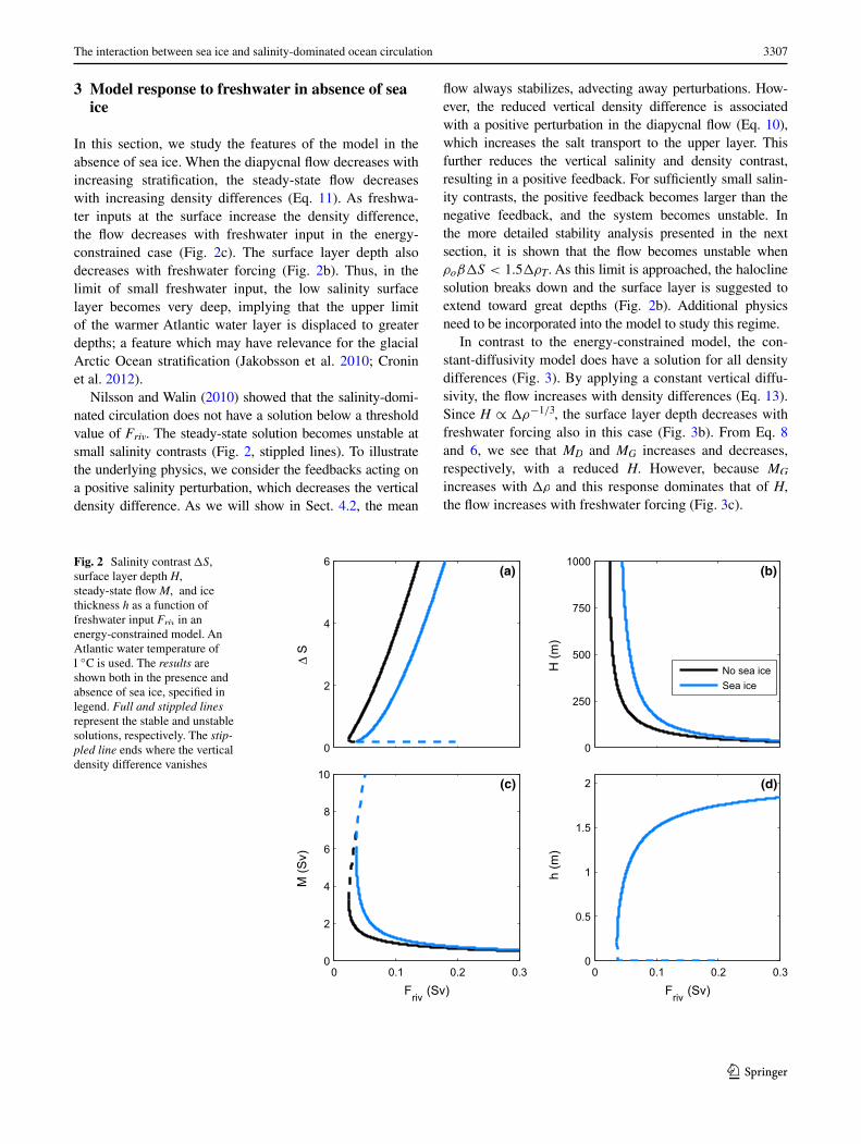
In contrast to the energy-constrained model, the con-stant-diffusivity model does have a solution for all density differences (Fig. 3). By applying a constant vertical diffu-sivity, the flow increases with density differences (Eq. 13). Since H ∝ �ρ−1/3, the surface layer depth decreases with freshwater forcing also in this case (Fig. 3b). From Eq. 8 and 6, we see that MD and MG increases and decreases, respectively, with a reduced H. However, because MG increases with �ρ and this response dominates that of H, the flow increases with freshwater forcing (Fig. 3c).

Fig. 2 Salinity contrast �S, surface layer depth H, steady-state flow M, and ice thickness h as a function of freshwater input Friv in an energy-constrained model. An Atlantic water temperature of 1◦C is used. The results are

shown both in the presence and absence of sea ice, specified in legend. Full and stippled lines represent the stable and unstable solutions, respectively. The stip-pled line ends where the vertical density difference vanishes

0

2

4

6

∆ S

(a)

0

250

500

750

1000H

(m)

(b)

No sea iceSea ice

0 0.1 0.2 0.30

2

4

6

8

10

Friv (Sv)

M (S

v)

(c)

0 0.1 0.2 0.30

0.5

1

1.5

2

Friv (Sv)

h (m

)

(d)

3308 M. F. Jensen et al.

1 3

4 Model response to freshwater in presence of sea ice

4.1 The steady‑state response of sea ice thickness to changes in freshwater supply

Here, we focus on the impact of freshwater supply on the steady-state sea ice thickness. The sea ice is linked to the freshwater supply via the heat flux from the ocean to the ice. The heat flux is proportional to M (Eq. 18). In essence, a stronger steady-state heat flux results in thinner sea ice. However, the thickness-dependent sea ice export affects the net freshwater forcing of the ocean. Therefore, the sea ice is dynamically coupled to the ocean circulation.

The energy-constrained model shows increasing sea ice thickness with increasing freshwater forcing (Fig. 2d). It is also evident that the steady-state sensitivity of the sea ice thickness depends on the strength of freshwater supply. At large freshwater inputs, the sea ice thickness is rather insensitive and large changes in the freshwater forcing are needed to change the sea ice thickness. On the other hand, for small freshwater inputs, only small changes in the freshwater forcing are needed to change the sea ice thick-ness drastically. It is worth noting that in the uncoupled sea ice model, thick sea ice is more sensitive to a given change in the forcing than thin ice (Bitz and Roe 2004). The same

basic physics still applies here, which reflects the fact that thinner ice grows faster. However, the sensitivity of the ocean heat flux becomes so strong at low freshwater sup-plies that it dominates over the thickness-dependent effect of sea ice growth.

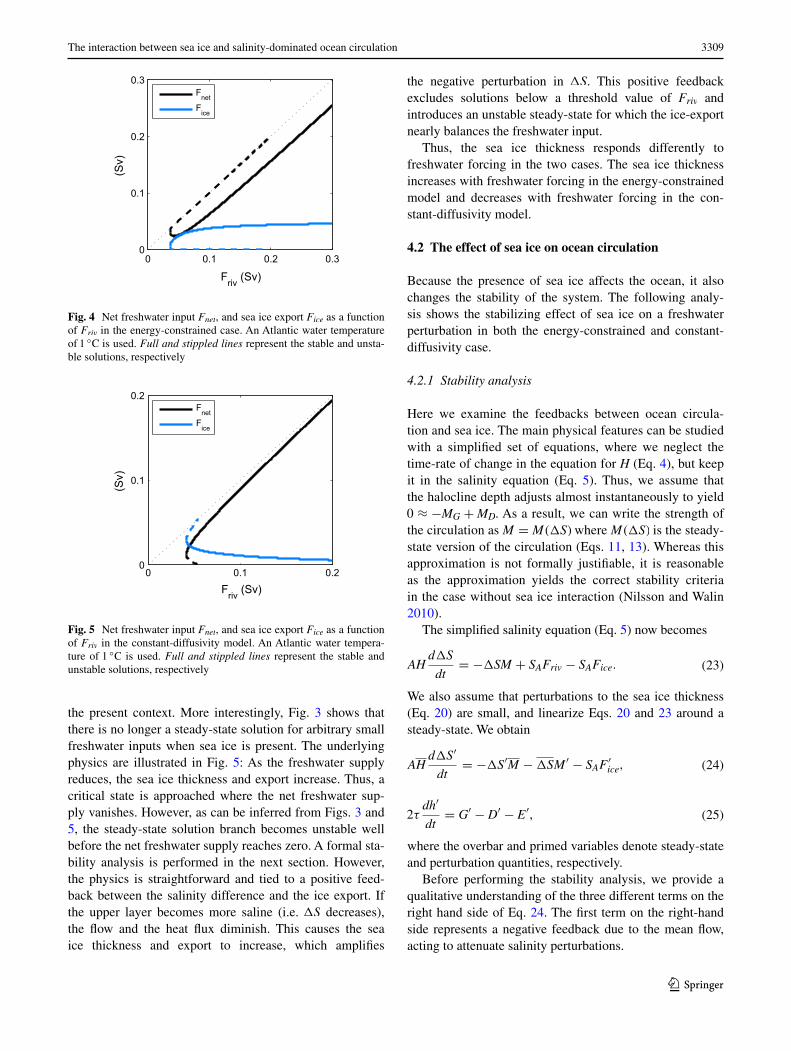
Figure 2a shows that for a given external freshwater input the salinity difference is lower in the presence of sea ice, i.e. the salinity of the upper layer is higher. This is a consequence of the sea ice export, which carries away part of the external freshwater input. For the energy-constrained model which only has steady-state solutions above a threshold value of the net freshwater input, the sea ice tends to extend the range of steady-states. However, the sea ice export actually limits the steady-states with respect to Friv (Fig. 2). Figure 4 illustrates how the net freshwater supply and freshwater exported by sea ice vary with the external freshwater input. For large inputs of Friv, the role of the sea ice in the freshwater budget is small. However, for small inputs of Friv, sea ice plays a leading order role for the freshwater budget.

In the constant-diffusivity case the sea ice response is essentially reversed. Here, the sea ice thins as the fresh-water supply increases (Fig. 3d). For a sufficiently large freshwater input, the sea ice will vanish. This transition to an ice-free state is gradual and continuous, and presum-ably requires too large freshwater inputs to be relevant in

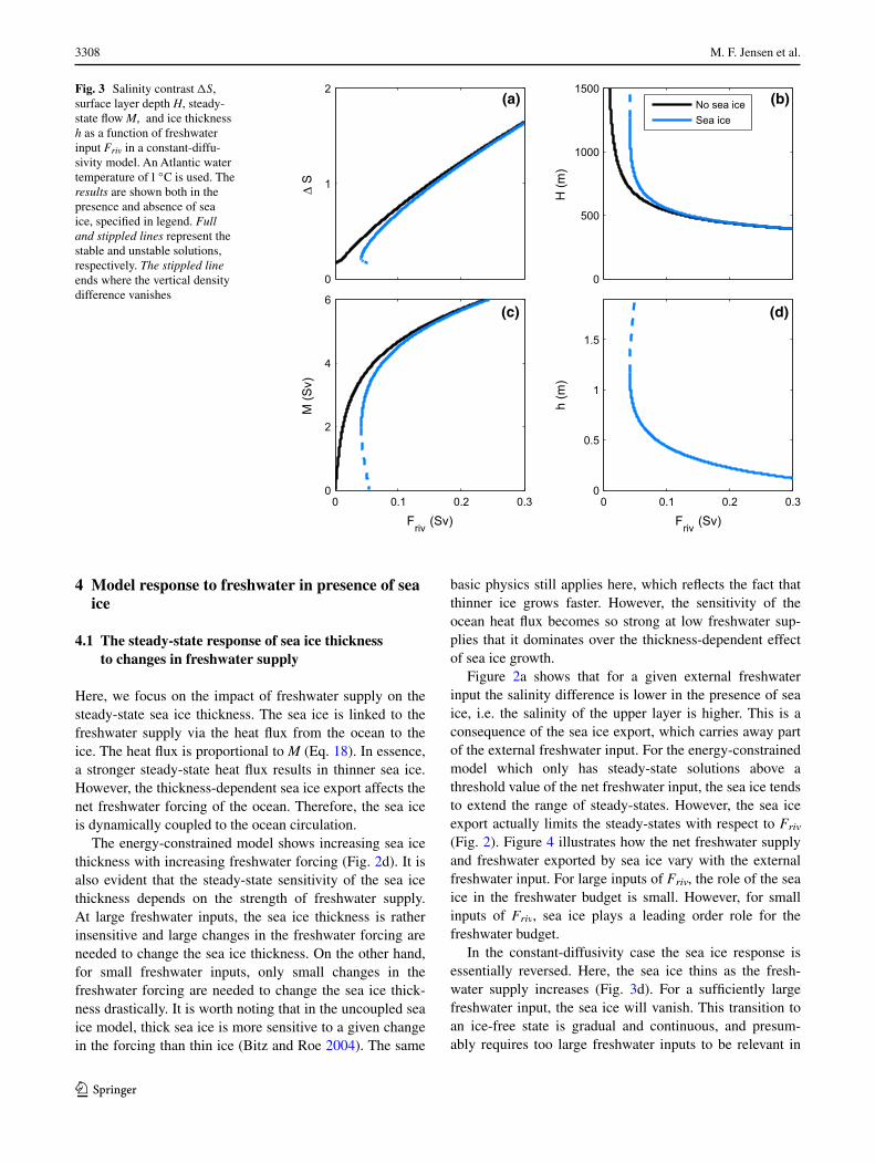
Fig. 3 Salinity contrast �S, surface layer depth H, steady-state flow M, and ice thickness h as a function of freshwater input Friv in a constant-diffu-sivity model. An Atlantic water temperature of 1 ◦

C is used. The results are shown both in the presence and absence of sea ice, specified in legend. Full and stippled lines represent the stable and unstable solutions, respectively. The stippled line ends where the vertical density difference vanishes

0

1

2(a)

∆ S

0

500

1000

1500(b)

H (m

)

No sea iceSea ice

0 0.1 0.2 0.30

2

4

6

Friv (Sv)

M (S

v)(c)

0 0.1 0.2 0.30

0.5

1

1.5

Friv (Sv)

h (m

)

(d)

3309The interaction between sea ice and salinity-dominated ocean circulation

1 3

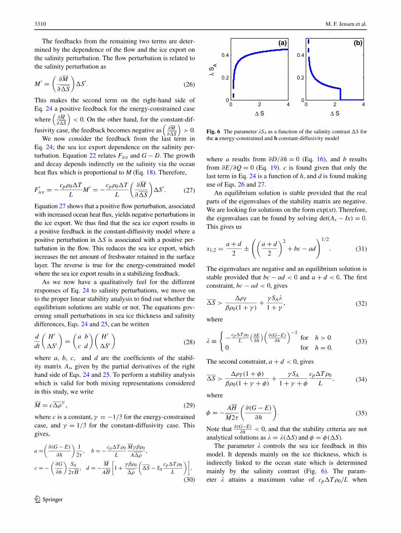
the present context. More interestingly, Fig. 3 shows that there is no longer a steady-state solution for arbitrary small freshwater inputs when sea ice is present. The underlying physics are illustrated in Fig. 5: As the freshwater supply reduces, the sea ice thickness and export increase. Thus, a critical state is approached where the net freshwater sup-ply vanishes. However, as can be inferred from Figs. 3 and 5, the steady-state solution branch becomes unstable well before the net freshwater supply reaches zero. A formal sta-bility analysis is performed in the next section. However, the physics is straightforward and tied to a positive feed-back between the salinity difference and the ice export. If the upper layer becomes more saline (i.e. �S decreases), the flow and the heat flux diminish. This causes the sea ice thickness and export to increase, which amplifies

the negative perturbation in �S. This positive feedback excludes solutions below a threshold value of Friv and introduces an unstable steady-state for which the ice-export nearly balances the freshwater input.

Thus, the sea ice thickness responds differently to freshwater forcing in the two cases. The sea ice thickness increases with freshwater forcing in the energy-constrained model and decreases with freshwater forcing in the con-stant-diffusivity model.

4.2 The effect of sea ice on ocean circulation

Because the presence of sea ice affects the ocean, it also changes the stability of the system. The following analy-sis shows the stabilizing effect of sea ice on a freshwater perturbation in both the energy-constrained and constant-diffusivity case.

4.2.1 Stability analysis

Here we examine the feedbacks between ocean circula-tion and sea ice. The main physical features can be studied with a simplified set of equations, where we neglect the time-rate of change in the equation for H (Eq. 4), but keep it in the salinity equation (Eq. 5). Thus, we assume that the halocline depth adjusts almost instantaneously to yield 0 ≈ −MG +MD. As a result, we can write the strength of the circulation as M = M(�S) where M(�S) is the steady-state version of the circulation (Eqs. 11, 13). Whereas this approximation is not formally justifiable, it is reasonable as the approximation yields the correct stability criteria in the case without sea ice interaction (Nilsson and Walin 2010).

The simplified salinity equation (Eq. 5) now becomes

We also assume that perturbations to the sea ice thickness (Eq. 20) are small, and linearize Eqs. 20 and 23 around a steady-state. We obtain

where the overbar and primed variables denote steady-state and perturbation quantities, respectively.

Before performing the stability analysis, we provide a qualitative understanding of the three different terms on the right hand side of Eq. 24. The first term on the right-hand side represents a negative feedback due to the mean flow, acting to attenuate salinity perturbations.

(23)AHd�S

dt= −�SM + SAFriv − SAFice.

(24)AHd�S′

dt= −�S′M −�SM ′

− SAF′ice,

(25)2τdh′

dt= G′

− D′− E′

,

0 0.1 0.2 0.30

0.1

0.2

0.3

(Sv)

Friv (Sv)

FnetFice

Fig. 4 Net freshwater input Fnet, and sea ice export Fice as a function of Friv in the energy-constrained case. An Atlantic water temperature of 1 ◦

C is used. Full and stippled lines represent the stable and unsta-ble solutions, respectively

0 0.1 0.20

0.1

0.2

(Sv)

Friv (Sv)

FnetFice

Fig. 5 Net freshwater input Fnet, and sea ice export Fice as a function of Friv in the constant-diffusivity model. An Atlantic water tempera-ture of 1 ◦

C is used. Full and stippled lines represent the stable and unstable solutions, respectively

3310 M. F. Jensen et al.

1 3

The feedbacks from the remaining two terms are deter-mined by the dependence of the flow and the ice export on the salinity perturbation. The flow perturbation is related to the salinity perturbation as

This makes the second term on the right-hand side of Eq. 24 a positive feedback for the energy-constrained case

where (

∂M

∂�S

)

< 0. On the other hand, for the constant-dif-

fusivity case, the feedback becomes negative as (

∂M

∂�S

)

> 0.

We now consider the feedback from the last term in Eq. 24; the sea ice export dependence on the salinity per-turbation. Equation 22 relates Fice and G− D. The growth and decay depends indirectly on the salinity via the ocean heat flux which is proportional to M (Eq. 18). Therefore,

Equation 27 shows that a positive flow perturbation, associated with increased ocean heat flux, yields negative perturbations in the ice export. We thus find that the sea ice export results in a positive feedback in the constant-diffusivity model where a positive perturbation in �S is associated with a positive per-turbation in the flow. This reduces the sea ice export, which increases the net amount of freshwater retained in the surface layer. The reverse is true for the energy-constrained model where the sea ice export results in a stabilizing feedback.

As we now have a qualitatively feel for the different responses of Eq. 24 to salinity perturbations, we move on to the proper linear stability analysis to find out whether the equilibrium solutions are stable or not. The equations gov-erning small perturbations in sea ice thickness and salinity differences, Eqs. 24 and 25, can be written

where a, b, c, and d are the coefficients of the stabil-ity matrix As, given by the partial derivatives of the right hand side of Eqs. 24 and 25. To perform a stability analysis which is valid for both mixing representations considered in this study, we write

where c is a constant, γ = −1/3 for the energy-constrained case, and γ = 1/3 for the constant-diffusivity case. This gives,

(26)M ′=

(

∂M

∂�S

)

�S′.

(27)F ′ice = −

cpρ0�T

LM ′

= −cpρ0�T

L

(

∂M

∂�S

)

�S′.

(28)d

dt

(

H ′

�S′

)

=

(

a b

c d

)(

H ′

�S′

)

(29)M = c�ργ,

(30)

a =

(

∂(G− E)

∂h

)

1

2τ, b = −

cp�Tρ0

L

Mγβρ0

A�ρ,

c =−

(

∂G

∂h

)

SA

2τH, d = −

M

AH

[

1+γβρ0

�ρ

(

�S − SAcp�Tρ0

L

)]

,

where a results from ∂D/∂h = 0 (Eq. 16), and b results from ∂E/∂Q = 0 (Eq. 19). c is found given that only the last term in Eq. 24 is a function of h, and d is found making use of Eqs. 26 and 27.

An equilibrium solution is stable provided that the real parts of the eigenvalues of the stability matrix are negative. We are looking for solutions on the form exp(xt). Therefore, the eigenvalues can be found by solving det(As − Ix) = 0. This gives us

The eigenvalues are negative and an equilibrium solution is stable provided that bc− ad < 0 and a+ d < 0. The first constraint, bc− ad < 0, gives

where

The second constraint, a+ d < 0, gives

where

Note that ∂(G−E)∂h

< 0, and that the stability criteria are not analytical solutions as � = �(�S) and φ = φ(�S).

The parameter � controls the sea ice feedback in this model. It depends mainly on the ice thickness, which is indirectly linked to the ocean state which is determined mainly by the salinity contrast (Fig. 6). The param-eter � attains a maximum value of cp�Tρ0/L when

(31)x1,2 =a+ d

2±

(

(

a+ d

2

)2

+ bc − ad

)1/2

.

(32)�S >�ρT

βρ0(1+ γ )+

γ SA�

1+ γ,

(33)� ≡

{

−cp�Tρ0

L

(

∂E∂h

)

(

∂(G−E)∂h

)−1

for h > 0

0 for h = 0.

(34)�S >�ρT (1+ φ)

βρ0(1+ γ + φ)+

γ SA

1+ γ + φ

cp�Tρ0

L,

(35)φ = −AH

M2τ

(

∂(G− E)

∂h

)

.

0 2 40

0.2

0.4

∆ S

λ S A

(a)

0 2 40

0.2

0.4

(b)

∆ S

Fig. 6 The parameter �SA as a function of the salinity contrast �S for the a energy-constrained and b constant-diffusivity model

3311The interaction between sea ice and salinity-dominated ocean circulation

1 3

(

∂E

∂h

)

≫

(

∂G

∂h

)

. For TA = 1◦C, that value is 0.0372. Due to

the thermodynamics of sea ice, the rate of sea ice growth decreases for thick ice, and � approaches its maximum for very thick sea ice. If sea ice export is insensitive to sea ice thickness, � is zero.

The parameter φ is essentially the ratio of the time scales for the response of the salinity and the sea ice. In the limit of fast sea ice response, φ approaches infinity, and the second stability criterion (Eq. 34) yields �S > �ρT/βρ0 which is always satisfied. In the limit of slow sea ice response, φ = 0. In this case, the second stability criterion is stricter when γ > 0. The first criterion applies for γ < 0 . For both representations of the diapycnal flow considered in this study, the first criterion determines where the solu-tion becomes unstable.

For the energy-constrained case where γ < 0, the sea ice feedback from the last term in Eq. 32 is negative, con-firming sea ice as a negative feedback. As the presence of sea ice stabilizes the circulation, while flow perturbations destabilize, it is interesting to see whether the presence of sea ice compensates for the destabilizing effects in the energy-constrained model. We get the stability criterion for the energy-constrained model �SE by inserting γ = −1/3 in Eq. 32;

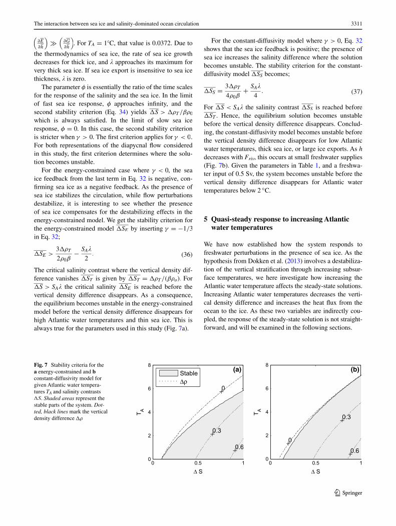
The critical salinity contrast where the vertical density dif-ference vanishes �ST is given by �ST = �ρT/(βρo). For �S > SA� the critical salinity �SE is reached before the vertical density difference disappears. As a consequence, the equilibrium becomes unstable in the energy-constrained model before the vertical density difference disappears for high Atlantic water temperatures and thin sea ice. This is always true for the parameters used in this study (Fig. 7a).

(36)�SE >3�ρT

2ρ0β−

SA�

2.

For the constant-diffusivity model where γ > 0, Eq. 32 shows that the sea ice feedback is positive; the presence of sea ice increases the salinity difference where the solution becomes unstable. The stability criterion for the constant-diffusivity model �SS becomes;

For �S < SA� the salinity contrast �SS is reached before �ST . Hence, the equilibrium solution becomes unstable before the vertical density difference disappears. Conclud-ing, the constant-diffusivity model becomes unstable before the vertical density difference disappears for low Atlantic water temperatures, thick sea ice, or large ice exports. As h decreases with Friv, this occurs at small freshwater supplies (Fig. 7b). Given the parameters in Table 1, and a freshwa-ter input of 0.5 Sv, the system becomes unstable before the vertical density difference disappears for Atlantic water temperatures below 2 ◦C.

5 Quasi‑steady response to increasing Atlantic water temperatures

We have now established how the system responds to freshwater perturbations in the presence of sea ice. As the hypothesis from Dokken et al. (2013) involves a destabiliza-tion of the vertical stratification through increasing subsur-face temperatures, we here investigate how increasing the Atlantic water temperature affects the steady-state solutions. Increasing Atlantic water temperatures decreases the verti-cal density difference and increases the heat flux from the ocean to the ice. As these two variables are indirectly cou-pled, the response of the steady-state solution is not straight-forward, and will be examined in the following sections.

(37)�SS =3�ρT

4ρ0β+

SA�

4.

Fig. 7 Stability criteria for the a energy-constrained and b constant-diffusivity model for given Atlantic water tempera-tures TA and salinity contrasts �S. Shaded areas represent the stable parts of the system. Dot-ted, black lines mark the vertical density difference �ρ

0 0.5 10

2

4

6

8

T A

∆ S

0

0.3

0.6

(b)

0 0.5 10

2

4

6

8

T A

∆ S

(a)

0

0.3

0.6

Stable∆ρ

3312 M. F. Jensen et al.

1 3

5.1 Energy‑constrained case

First, we study the dynamic response of the steady-state flow to increasing TA. We recall that M intensifies with decreasing density differences in the energy-constrained case (Eq. 11).

The stronger ocean flow advects more saline water into the surface layer, thereby reducing the salinity contrast (Fig. 8, inner loop). In addition, the value of the critical salinity con-trast increases with Atlantic water temperatures (Eq. 36). The dynamic response to increasing Atlantic water tempera-tures is therefore to decrease the stability of the system by driving the system toward the critical salinity contrast where the steady-state solution becomes unstable.

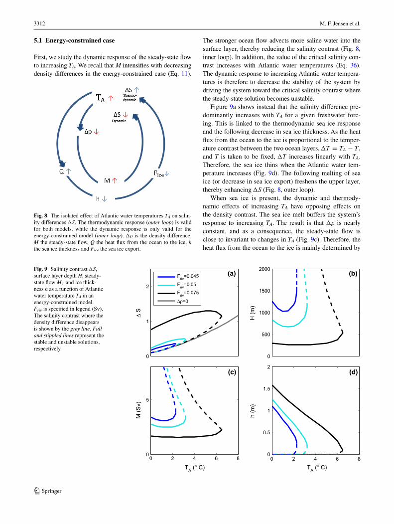
Figure 9a shows instead that the salinity difference pre-dominantly increases with TA for a given freshwater forc-ing. This is linked to the thermodynamic sea ice response and the following decrease in sea ice thickness. As the heat flux from the ocean to the ice is proportional to the temper-ature contrast between the two ocean layers, �T = TA − T , and T is taken to be fixed, �T increases linearly with TA . Therefore, the sea ice thins when the Atlantic water tem-perature increases (Fig. 9d). The following melting of sea ice (or decrease in sea ice export) freshens the upper layer, thereby enhancing �S (Fig. 8, outer loop).

When sea ice is present, the dynamic and thermody-namic effects of increasing TA have opposing effects on the density contrast. The sea ice melt buffers the system’s response to increasing TA. The result is that �ρ is nearly constant, and as a consequence, the steady-state flow is close to invariant to changes in TA (Fig. 9c). Therefore, the heat flux from the ocean to the ice is mainly determined by

Fig. 8 The isolated effect of Atlantic water temperatures TA on salin-ity differences �S. The thermodynamic response (outer loop) is valid for both models, while the dynamic response is only valid for the energy-constrained model (inner loop). �ρ is the density difference, M the steady-state flow, Q the heat flux from the ocean to the ice, h the sea ice thickness and Fice the sea ice export.

Fig. 9 Salinity contrast �S, surface layer depth H, steady-state flow M, and ice thick-ness h as a function of Atlantic water temperature TA in an energy-constrained model. Friv is specified in legend (Sv). The salinity contrast where the density difference disappears is shown by the grey line. Full and stippled lines represent the stable and unstable solutions, respectively

0

1

2

∆ S

(a)Friv=0.045

Friv=0.05

Friv=0.075

∆ρ=0

0

500

1000

1500

2000(b)

H (m

)

0 2 4 6 80

0.5

1

1.5

2(d)

h (m

)

0 2 4 6 80

5

(c)

TA (° C) TA (° C)

M (S

v)

3313The interaction between sea ice and salinity-dominated ocean circulation

1 3

�T in the energy-constrained case. However, when the sea ice thins sufficiently, the effect of melting is too small to balance the increase in TA with respect to the density con-trast. At that point, �ρ decreases with TA. Therefore, as h approaches zero, M increases sharply with TA. As a conse-quence, the salinity contrast decreases with Atlantic water temperatures when h is small (Fig. 9a, d). At this point, high Atlantic water temperatures destabilize the system. The sea ice feedback, which is controlled by � (Eq. 33), is not strong enough to balance the destabilizing effect of the flow.

Due to the destabilizing effect of the flow, the steady-state solution becomes unstable at high Atlantic water tem-peratures (Fig. 9). For low freshwater inputs, this occurs at salinity contrasts where sea ice still is present. As a con-sequence, the sea ice abruptly disappears (Fig. 9d). For higher freshwater inputs, the steady-state solution turns unstable as the sea ice disappears due to the removal of the stabilizing effect of the sea ice (not shown). For all values, the system turns unstable before the vertical density differ-ence disappears (Fig. 7).

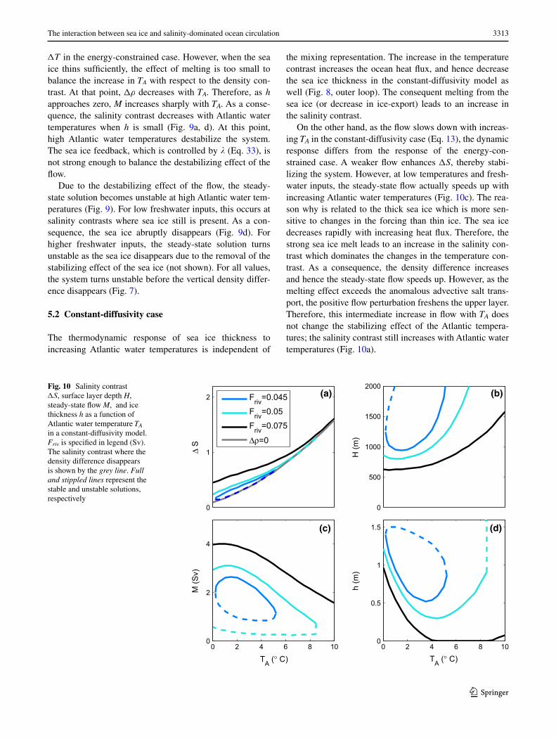
5.2 Constant‑diffusivity case

The thermodynamic response of sea ice thickness to increasing Atlantic water temperatures is independent of

the mixing representation. The increase in the temperature contrast increases the ocean heat flux, and hence decrease the sea ice thickness in the constant-diffusivity model as well (Fig. 8, outer loop). The consequent melting from the sea ice (or decrease in ice-export) leads to an increase in the salinity contrast.

On the other hand, as the flow slows down with increas-ing TA in the constant-diffusivity case (Eq. 13), the dynamic response differs from the response of the energy-con-strained case. A weaker flow enhances �S, thereby stabi-lizing the system. However, at low temperatures and fresh-water inputs, the steady-state flow actually speeds up with increasing Atlantic water temperatures (Fig. 10c). The rea-son why is related to the thick sea ice which is more sen-sitive to changes in the forcing than thin ice. The sea ice decreases rapidly with increasing heat flux. Therefore, the strong sea ice melt leads to an increase in the salinity con-trast which dominates the changes in the temperature con-trast. As a consequence, the density difference increases and hence the steady-state flow speeds up. However, as the melting effect exceeds the anomalous advective salt trans-port, the positive flow perturbation freshens the upper layer. Therefore, this intermediate increase in flow with TA does not change the stabilizing effect of the Atlantic tempera-tures; the salinity contrast still increases with Atlantic water temperatures (Fig. 10a).

Fig. 10 Salinity contrast �S, surface layer depth H, steady-state flow M, and ice thickness h as a function of Atlantic water temperature TA in a constant-diffusivity model. Friv is specified in legend (Sv). The salinity contrast where the density difference disappears is shown by the grey line. Full and stippled lines represent the stable and unstable solutions, respectively

0

1

2 (a)

∆ S

Friv=0.045

Friv=0.05

Friv=0.075

∆ρ=0

0 2 4 6 8 100

0.5

1

1.5 (d)

TA (° C)

h (m

)

0 2 4 6 8 100

2

4

(c)

TA (° C)

M (S

v)

0

500

1000

1500

2000(b)

H (m

)

3314 M. F. Jensen et al.

1 3

In the constant-diffusivity case, the sea ice thickness response depends on the competing effects of the dynamic and thermodynamic responses to increasing TA. The heat flux is proportional to �TM, and the two terms have oppos-ing effects on the heat flux as the steady-state flow mainly decreases with TA (Fig. 10c). Interestingly, we get a local minimum in sea ice thickness with increasing TA (Fig. 10d). This occurs when the decrease in M balances the increase in �T , i.e., when the dynamic and thermodynamic effects are equal. When the decrease in the steady-state flow is large enough to dominate changes in the temperature con-trast, the heat flux decreases with increasing TA. The result is an increase in h with increasing Atlantic water tempera-tures at large TA (Fig. 10d).

The change in the response of the sea ice to increasing Atlantic water temperatures changes the stability prop-erties of the system. At low freshwater inputs the steady-state solution becomes unstable at low Atlantic water tem-peratures (Fig. 10, blue line, and Fig. 7). This is due to the thick sea ice and large ice-export which removes most of the freshwater introduced to the surface layer. By increas-ing TA, steady-state solutions are introduced as the sea ice melt stabilizes the system. However, at higher Atlantic water temperatures, where sea ice thickens with TA, the sea ice growth acts destabilizing. At high Atlantic water tem-peratures, the ice export dominates the freshwater input and flow perturbations, and the system becomes unstable. Note that the salinity contrast still increases at high tem-peratures due to a weaker flow (Fig. 10a). However, due to thicker sea ice and a larger �, so does the salinity contrast where the steady-state solution becomes unstable (Eq. 37). Interestingly, the system becomes unstable at both high and low Atlantic water temperatures for low freshwater inputs

(Fig. 10, blue line). For high freshwater inputs, the system stays stable until the vertical density difference disappears (Fig. 7).

We have shown that the system can turn unstable at high Atlantic water temperatures for both mixing representa-tions, depending on the freshwater input. What happens at this point goes beyond the physics contained in the present version of our model. Still, it is fair to assume that the sea ice suddenly disappears as a new regime is established.

6 Discussion

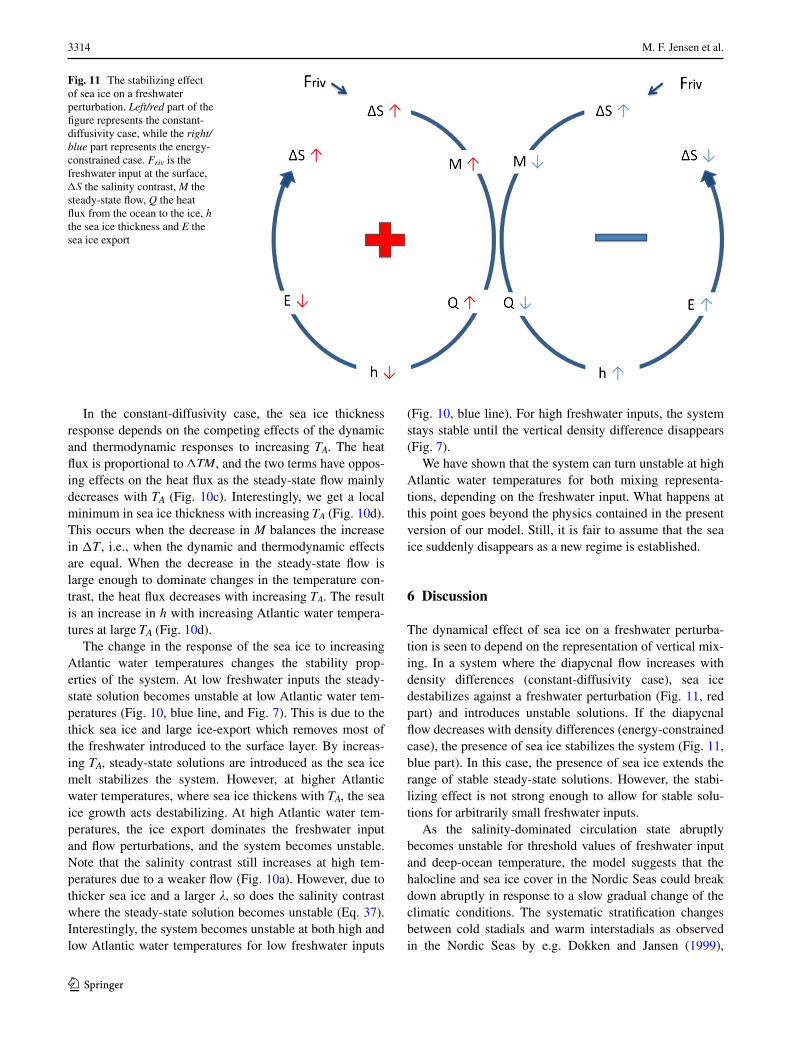
The dynamical effect of sea ice on a freshwater perturba-tion is seen to depend on the representation of vertical mix-ing. In a system where the diapycnal flow increases with density differences (constant-diffusivity case), sea ice destabilizes against a freshwater perturbation (Fig. 11, red part) and introduces unstable solutions. If the diapycnal flow decreases with density differences (energy-constrained case), the presence of sea ice stabilizes the system (Fig. 11, blue part). In this case, the presence of sea ice extends the range of stable steady-state solutions. However, the stabi-lizing effect is not strong enough to allow for stable solu-tions for arbitrarily small freshwater inputs.

As the salinity-dominated circulation state abruptly becomes unstable for threshold values of freshwater input and deep-ocean temperature, the model suggests that the halocline and sea ice cover in the Nordic Seas could break down abruptly in response to a slow gradual change of the climatic conditions. The systematic stratification changes between cold stadials and warm interstadials as observed in the Nordic Seas by e.g. Dokken and Jansen (1999),

Fig. 11 The stabilizing effect of sea ice on a freshwater perturbation. Left/red part of the figure represents the constant-diffusivity case, while the right/blue part represents the energy-constrained case. Friv is the freshwater input at the surface, �S the salinity contrast, M the steady-state flow, Q the heat flux from the ocean to the ice, h the sea ice thickness and E the sea ice export

3315The interaction between sea ice and salinity-dominated ocean circulation

1 3

Rasmussen and Thomsen (2004) and Dokken et al. (2013) can be explained by a reduction in the freshwater supply to the Nordic Seas. This is highly relevant for a cold, gla-cial climate with a weaker hydrological cycle. Generally, we expect reduced input of freshwater to the Nordic Seas during cold, stadial conditions. In this case, only a small change in the freshwater supply is needed to initiate large and abrupt changes in both sea ice and ocean stratification (Fig. 2). This can be contrasted to the traditional freshwa-ter hosing experiments where a large additional freshwa-ter forcing of about 1 Sv to the North Atlantic is applied to maintain cold stadial conditions with extensive sea ice cover (e.g. Manabe and Stouffer 1995; Stouffer et al. 2006). In this case, an abrupt termination of the freshwater forcing is required to trigger a transition to a warm interstadial with weak stratification and reduced sea ice (Liu et al. 2009).

The abrupt changes in sea ice and ocean stratification at small freshwater supplies can occur independently of a change in subsurface temperature. However, the simple model also transitions to an unstable solution with a removal of sea ice when the temperature of the subsurface Atlantic water is increased (Fig. 9d). This is similar to the hypoth-esized transition from cold stadial states to warm intersta-dials triggered by warm Atlantic water as in Dokken et al. (2013). Interestingly, the unstable state is reached before the vertical density difference disappears. This is mainly true for the energy-constrained case. For the constant-diffusivity case, the stable solutions disappear for both high and low Atlantic water temperatures when the freshwater supply is low. At higher freshwater supplies, the system stays stable until the vertical density difference disappears. However, we recall that the constant-diffusivity model may be a less real-istic representation of the system and is not thought of as a good analogue for the Nordic Seas/Arctic.

For the energy-constrained case, at low freshwater inputs, only a small increase in temperature is needed to destabilize the equilibrium state, and as a consequence, sea ice abruptly disappears. As both increasing Atlantic water temperatures and decreasing freshwater inputs promote an unstable system, the removal of the halocline as proposed by Dokken et al. (2013), can occur with smaller changes in Atlantic water temperatures than previously thought.

Our results are highly dependent on the use of a thick-ness dependent sea ice export. If we instead assume that the ice-export is constant and independent of the ice thickness (not shown), then the sea ice related feedbacks on the flow and the salinity stratification vanish. The equilibrium states become unstable at the same salinity contrast as when sea ice is absent. However, as the ice-export reduces the salin-ity contrast for a given freshwater input, the system with stability-dependent mixing still becomes unstable at a larger freshwater input in the presence of sea ice.

As the present conceptual model is highly simplified and essentially one-dimensional, it neglects several pro-cesses that could be of importance for the dynamics of the halocline and sea ice. In particular, the model does not rep-resent effects of wind forcing on either the ocean circula-tion or the sea ice export. Possible impacts of ice mechan-ics are also ignored in the parametrization of the sea ice export, which simply is taken as proportional to the sea ice thickness. Note further that even though the sea ice model crudely represents an annual growth and melt cycle, effects of seasonal changes in the freshwater storage due to growth and melt of sea ice are not accounted for in the model. Adding representations of seasonality and natural variability can obviously change the stability range of the steady-state solutions examined here. Reductions in air-sea momentum exchange for high sea ice concentrations could also affect the stability properties of the system. In the presence of sea ice, the energy input from the atmosphere to oceanic mixing via e.g. internal wave generation should diminish (Rainville and Woodgate 2009). Thus, the energy supply to the vertical mixing ǫ would hence decrease. In the energy-constrained model this would introduce a feedback between the strength of the flow and the sea ice concentra-tion, with ensuing impacts on the stability of the system.

The results from our simple model suggest a mechanism for how a reduction in freshwater input to the Nordic Seas could initiate large changes in the sea ice cover. Due to the instability at small freshwater supplies, small changes in the freshwater input or increases in subsurface tempera-tures could terminate the salinity-dominated mode with sea ice, and allow for a less stratified regime without sea ice. This could aid in explaining why the sea ice and hydrog-raphy of the Nordic Seas were highly variable during the last glacial cycle. Our simple model only accounts for the retreat of the sea ice cover, and does not provide any mech-anism for the re-appearance of sea ice in the Nordic Seas.

7 Conclusion

The main results from the examination of the conceptual model of sea ice-ocean-circulation feedbacks are:

–– The presence of sea ice stabilizes against a freshwater perturbation when the vertical velocity is represented with a constant energy-supply to the diffusivity.

–– The presence of sea ice destabilizes against a freshwa-ter perturbation when the vertical velocity is represented with a constant diffusivity.

–– For sufficiently weak freshwater supply and irrespective of the representation of the vertical mixing, the salinity-dominated circulation becomes unstable.

3316 M. F. Jensen et al.

1 3

–– The sea ice is highly sensitive to changes in subsurface Atlantic water temperatures.

–– The results from the simple conceptual model sug-gest that during cold glacial conditions, with reduced input of freshwater to the Nordic Seas, relatively small changes in freshwater or Atlantic water temperature could have triggered abrupt transitions in sea ice cover.

Acknowledgments The research was supported by the Centre for Climate Dynamics at the Bjerknes Centre. The research leading to these results is part of the ice2ice project funded by the European Research Council under the European Community’s Seventh Frame-work Programme (FP7/2007-2013)/ERC Grant Agreement No. 610055. J. Nilsson acknowledges support from the Swedish National Space Board, the Knut and Alice Wallenberg Foundation (via the SWERUS-C3 program), and the Bolin Centre for Climate Research at Stockholm University. We thank the anonymous reviewers for their constructive comments which greatly improved the manuscript.

Open Access This article is distributed under the terms of the Creative Commons Attribution 4.0 International License (http://crea-tivecommons.org/licenses/by/4.0/), which permits unrestricted use, distribution, and reproduction in any medium, provided you give appropriate credit to the original author(s) and the source, provide a link to the Creative Commons license, and indicate if changes were made.

References

Arzel O, Colin de Verdiere A, England MH (2010) The role of oce-anic heat transport and wind stress forcing in abrupt millennial-scale climate transitions. J Clim 23:2233–2256

Bitz CM, Roe GH (2004) A mechanism for high rate of sea ice thin-ning in the Arctic Ocean. J Clim 17:3623–3632

Broecker WS (2000) Abrupt climate change: casual constraints pro-vided by the paleoclimate record. Earth-Sci Rev 51:137–154

Broecker WS, Bond G, Klas M (1990) A salt oscillator in the glacial Atlantic? 1: the concept. Paleoceanography 5:469–477

Bryan F (1986) High-latitude salinity effects and interhemispheric thermohaline circulations. Nature 323:301–323

Colin de Verdiere A, Raa LT (2010) Weak oceanic heat transport as a cause of the instability of glacial climates. Clim Dyn 35(7–8):1237–1256. doi:10.1007/s00382-009-0675-8

Cronin TM, Dwyer GS, Farmer J, Bauch HA, Spielhagen RF, Jakobs-son M, Nilsson J, Briggs WM, Stepanova A (2012) Deep Arc-tic Ocean warming during the last glacial cycle. Nat Geosci 5:631–634

Dansgaard W, Johnsen SJ, Clausen HB, Dahl-Jensen D, Gundestrup NS, Hammer CU, Hvidberg CS, Steffensen JP, Sveinbjörnsdottir AE, Jouzel J, Bond G (1993) Evidence for general instability of past climate from a 250-kyr ice-core record. Nature 364:218–220

Dokken T, Jansen E (1999) Rapid changes in the mechanism of ocean convection during the last glacial period. Nature 401:458–461

Dokken TM, Nisancioglu KH, Li C, Battisti DS, Kissel C (2013) Dansgaard–Oeschger cycles: interactions between ocean and sea intrinsic to the Nordic Seas. Paleoceanography 28:491–502

Fanning AF, Weaver AJ (1997) Temporal-geographical meltwater influences on the North Atlantic conveyor: implications for the younger dryas. Paleoceanography 12:307–320

Ganopolski A, Rahmstorf S (2001) Rapid changes of glacial climate simulated in a coupled climate model. Nature 409:153–158

Ganopolski A, Rahmstorf F (2002) Abrupt glacial climate changes due to stochastic resonance. Phys Rev Lett 88:038501

Gildor H, Tziperman E (2003) Sea-ice switches and abrupt climate change. Philos Trans R Soc London Ser A 361:1935–1944

Gnanadesikan A (1999) A simple predictive model for the structure of the oceanic pycnocline. Science 283:2077–2079

Guan YP, Huang RX (2008) Stommel’s box model of thermohaline circulation revisited: the role of mechanical energy support-ing mixing and the wind-driven gyration. J Phys Oceanogr 38:909–917

Huang R (1999) Mixing and energetics of the oceanic thermohaline circulation. J Phys Oceanogr 29(4):727–746

Jakobsson M, Nilsson J, Oregan M, Backman J, Lowemark L, Dowdeswell JA, Mayer L, Polyak L, Colleoni F, Anderson LG, Björk G, Darby D, Eriksson B, Hanslik D, Hell B, Marcussen C, Sellen E, Wallin A (2010) An Arctic Ocean ice shelf during MIS 6 constrained by new geophysical and geological data. Quat Sci Rev 29:3505–3517

Jayne SR, Marotzke J (1999) A destabilizing thermohaline circula-tion-atmosphere-sea ice feedback. J Clim 12:642–651

Johnson HL, Marshall DP, Sproson DAJ (2007) Reconciling theories of a mechanically driven meridional overturning circulation and multiple equilibria. Clim Dyn 29:821–836

Kato H, Phillips OM (1969) On the penetration of a turbulent layer into stratified fluid. J Fluid Mech 37:643–655

Knudsen M (1900) Ein hydrographischer lehrsatz. Ann Hydrogr Mar-itimen Meteor 28:316–320

Li C, Battisti DS, Schrag DP, Tziperman E (2005) Abrupt climate shifts in Greenland due to displacements of the sea ice edge. Geophys Res Lett 32(L19):702. doi:10.1029/2005GL023,492

Li C, Battisti DS, Bitz CM (2010) Can North Atlantic sea ice anoma-lies account for Dansgaard-Oeschger climate signals? J Clim 23:5457–5475

Liu Z, Otto-Bliesner B, He F, Brady E, Tomas R, Clark P, Carlson A, Lynch-Stieglitz J, Curry W, Brook E, Erickson D, Jacob R, Kutzbach J, Cheng J (2009) Transient simulation of last degla-ciation with a new mechanism for bølling-allerød warming. Sci-ence 325:310–314

Longworth H, Marotzke J, Stocker TF (2005) Ocean gyres and abrupt climate change in the thermohaline circulation: a conceptual analysis. J Clim 18:2403–2416

Lyle M (1997) Could early Cenozoic thermohaline circulation have warmed the poles? Paleoceanography 12:161–167

Manabe S, Stouffer RJ (1995) Simulation of abrupt climate change induced by freshwater input to the North Atlantic Ocean. Nature 378:165–167

Marotzke J (1989) Instabilities and multiple steady states of the ther-mohaline circulation. In: Anderson DLT, Willebrand J (eds) Oceanic circulation models: Combining data and dynamics. Springer, Netherlands, pp 501–511

Marotzke J (2000) Abrupt climate change and the thermohaline cir-culation: mechanisms and predictability. P Natl Acad Sci USA 97:1347–1350

Masson-Delmotte V, Jouzel J, Landais A, Stievenard M, Johnsen SJ, White JWC, Werner M, Sveinbjornsdottir A, Fuhrer K (2005) GRIP deuterium excess reveals rapid and orbital-scale changes in Greenland moisture origin. Science 309:118–121

Mayewski PA, Meeker LD, Twickler MS, Whitlow SI, Yang Q, Lyons WB, Prentice M (1997) Major features and forcing of high lati-tude northern hemisphere atmospheric circulation over the last 110,000 years. J Geophys Res 102:26,345–26,366

Munk WH (1966) Abyssal recipes. Deep-Sea Res 13:707–730Nilsson J, Walin G (2001) Freshwater forcing as a booster of thermo-

haline circulation. Tellus 53A:629–641Nilsson J, Walin G (2010) Salinity-dominated thermohaline circulation

in sill basins: Can two stable equilibria exist? Tellus 62A:123–133

3317The interaction between sea ice and salinity-dominated ocean circulation

1 3

Nilsson J, Björk G, Rudels B, Winsor P, Torres D (2008) Liquid fresh-water transport and polar surface water characteristics in the East Geenland current during the AO-02 Oden expedition. Prog Oceanogr 78:45–57

Park YG, Bryan K (2000) Comparison of thermally driven circulation from a depth-coordinate model and an isopycnal model. part i: scaling-law sensitivity to vertical diffusivity. J Phys Oceanogr 30:590–605

Peterson LC, Haug GH, Hughen KA, Rohl U (2000) Rapid changes in the hydrologic cycle of the tropical Atlantic during the last glacial. Science 290:1947–1951

Rainville L, Woodgate RA (2009) Observations of internal wave generation in the seasonally ice-free arctic. Geophys Res Lett 36(23):L23,604. doi:10.1029/2009GL041291

Rasmussen TL, Thomsen E (2004) The role of the North Atlantic Drift in the millennial timescale glacial climate fluctuations. Pal-aeogeogr Palaeoclimatol Palaeoecol 210:101–116

Sevellec F, Fedorov AV (2015) Unstable AMOC during glacial inter-vals and millennial variability: the role of mean sea ice extent. Earth Planet Sci Lett 429:60–68. doi:10.1016/j.epsl.2015.07.022

Severinghaus JP, Brook EJ (1999) Abrupt climate change at the end of the last glacial period inferred from trapped air in polar ice. Science 286:930–934

Stigebrandt A (1981) A model for the thickness and salinity of the upper layer in the Arctic Ocean and the relationship between the ice thickness and some external parameters. J Phys Oceanogr 11:1407–1422

Stocker TF, Wright DG (1991) Rapid transitions of the ocean’s deep circulation induced by changes in surface water fluxes. Nature 351:729–732

Stommel HM (1961) Thermohaline convection with two stable regimes of flow. Tellus 13:224–230

Stouffer RJ, Yin J, Gregory JM, Dixon KW, Spelman MJ, Hurlin W, Weaver AJ, Eby M, Flato GM, Hasumi H, Hu A, Jungclaus JH, Kamenkovich IV, Levermann A, Montoya M, Murakami S, Naw-rath S, Oka A, Peltier WR, Robitaille DY, Sokolov A, Vettoretti G, Weber SL (2006) Investigating the causes of the response of

the thermohaline circulation to past and future climate changes. J Clim 19(8):1365–1387. http://dx.doi.org/10.1175/JCLI3689.1

Stranne C, Björk G (2012) On the Arctic Ocean ice thickness response to changes in the external forcing. Clim Dyn 39:3007–3018

Thorndike AS (1992) A toy model linking atmospheric thermal radia-tion and sea ice growth. J Geophys Res 97:9401–9410

Timmermann A, Gildor H, Schulz M, Tziperman E (2003) Coherent resonant millennial-scale climate oscillations triggered by mas-sive meltwater pulses. J Clim 16:2569–2585

Tziperman E (1997) Inherently unstable climate behaviour due to weak thermohaline ocean circulation. Nature 386:592–595

Vallis GK (2006) Atmospheric and oceanic fluid dynamics: funda-mentals and large-scale circulation, 1st edn. Cambridge Univer-sity Press, Cambridge

Welander P (1971) The thermocline problem. Philos Trans R Soc Lond A 270:415–421

Welander P (1986) Thermohaline effects in the ocean circulation andrelated simple models. In: Willebrand J, Anderson DLT (eds) Large-scale transport processes in the oceans and atmosphrere. D.Reidel, Holland

Winton M (1993) Deep decoupling oscillations of the oceanic ther-mohaline circulation, in Ice in the climate system. Springer Ver-lag, Berlin

Winton M, Sarachik ES (1993) Thermohaline oscillations induced by strong steady salinity forcing of ocean general circulation mod-els. J Phys Oceanogr 23:1389–1410

Yang J, Neelin JD (1993) Sea-ice interaction with the thermohaline circulation. Geophys Res Lett 20:217–220

Yang J, Neelin JD (1997) Sea-ice interaction and the stability of the thermohaline circulation. Atmos-Ocean 35(4):433–469

Yu EF, Francois F, Bacon M (1996) Similar rates of modern and last-glacial ocean thermohaline circulation inferred from radiochemi-cal data. Nature 379:689–694

Zhang J, Schmitt RW, Huang RX (1999) The relative influence of diapycnal mixing and hydrological forcing on the stability of thermohaline circulation. J Phys Oceanogr 29:1096–1108