The Initial Value Problem - Cornell University

Chapter 9

The Initial Value Problem

§9.1 Basic Concepts

§9.2 The Runge-Kutta Methods

§9.3 The Adams Methods

The goal in the initial value problem (IVP) is to find a function y(t) given its value at some initial timet0 and a recipe f(t, y) for its slope:

y′(t) = f(t, y(t)), y(t0) = y0.

In applications we may want to plot an approximation to y(t) over a designated interval of interest [t0, tmax]in an effort to discover qualitative properties of the solution. Or we may require a highly accurate estimateof y(t) at some single, prescribed value t = T .

The methods we develop produce a sequence of solution snapshots (t1, y1), (t2, y2), . . . that are regardedas approximations to (t1, y(t1), (t2, y(t2)), etc. All we have at our disposal is the “slope function” f(t, y), bestthought of as a Matlab function f(t,y), that can be called whenever we need information about wherey(t) is “headed.” IVP solvers differ in how they use the slope function.

In §9.1 we use the Euler methods to introduce the basic ideas associated with approximate IVP solving:discretization, local error, global error, stability, etc. In practice the IVP usually involves a vector of unknownfunctions, and the treatment of such problems is also covered in §9.1. In this setting the given slope functionf(t, y) is a vector of scalar slope functions, and its evaluation tells us how each component in the unknowny(t) vector is changing with t.

The Runge-Kutta and Adams methods are then presented in §9.2 and §9.3 together with the built-inMatlab IVP solvers ode23 and ode45. We also discuss stepsize control, a topic of great practical importanceand another occasion to show off the role of calculus-based heuristics in scientific computing.

Quality software for the IVP is very complex. Years of research and development stand behind codes likeode23 and ode45. The implementations that we develop in this chapter are designed to build intuition and,if anything, are just the first step in the long journey from textbook formula to production software.

9.1 Basic Concepts

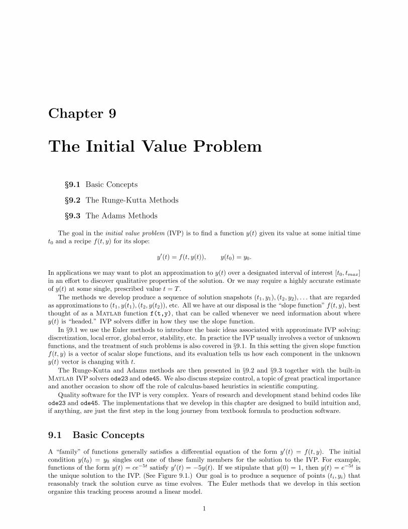
A “family” of functions generally satisfies a differential equation of the form y′(t) = f(t, y). The initialcondition y(t0) = y0 singles out one of these family members for the solution to the IVP. For example,functions of the form y(t) = ce−5t satisfy y′(t) = −5y(t). If we stipulate that y(0) = 1, then y(t) = e−5t isthe unique solution to the IVP. (See Figure 9.1.) Our goal is to produce a sequence of points (ti, yi) thatreasonably track the solution curve as time evolves. The Euler methods that we develop in this sectionorganize this tracking process around a linear model.

1

2 CHAPTER 9. THE INITIAL VALUE PROBLEM

−0.1 −0.05 0 0.05 0.1 0.15 0.2 0.25 0.3 0.35 0.40

0.2

0.4

0.6

0.8

1

1.2

1.4

1.6

1.8

2Solutions to y’(t) = −5 y(t)

Figure 9.1 Solution curves

9.1.1 Derivation of the Euler Method

From the initial condition, we know that (t0, y0) is on the solution curve. At this point the slope of thesolution is computable via the function f :

f0 = f(t0 , y0).

To estimate y(t) at some future time t1 = t0 + h0 we consider the following Taylor expansion:

y(t0 + h0) ≈ y(t0) + h0y′(t0) = y0 + h0f(t0 , y0).

This suggests that we use

y1 = y0 + h0f(t0 , y0)

as our approximation to the solution at time t1. The parameter h0 > 0 is the step, and it can be said thatwith the production of y1 we have “integrated the IVP forward” to t = t1.

With y1 ≈ y(t1) in hand, we try to push our knowledge of the solution one step further into the future.Let h1 be the next step. A Taylor expansion about t = t1 says that

y(t1 + h1) ≈ y(t1) + h1y′(t1) = y(t1) + h1f(t1 , y(t1)).

Note that in this case the right-hand side is not computable because we do not know the exact solution att = t1. However, if we are willing to use the approximations

y1 ≈ y(t1)

and

f1 = f(t1 , y1) ≈ f(t1, y(t1)),

then at time t2 = t1 + h1 we have

y(t2) ≈ y2 = y1 + h1f1.

The pattern is now clear. At each step we evaluate f at the current approximate solution point (tn, yn) andthen use that slope information to get yn+1. The key equation is

yn+1 = yn + hnf(tn , yn),

and its repeated application defines the Euler method:

9.1. BASIC CONCEPTS 3

n = 0Repeat:

fn = f(tn, yn)Determine the step hn > 0 and set tn+1 = tn + hn.yn+1 = yn + hnfn.

n = n + 1

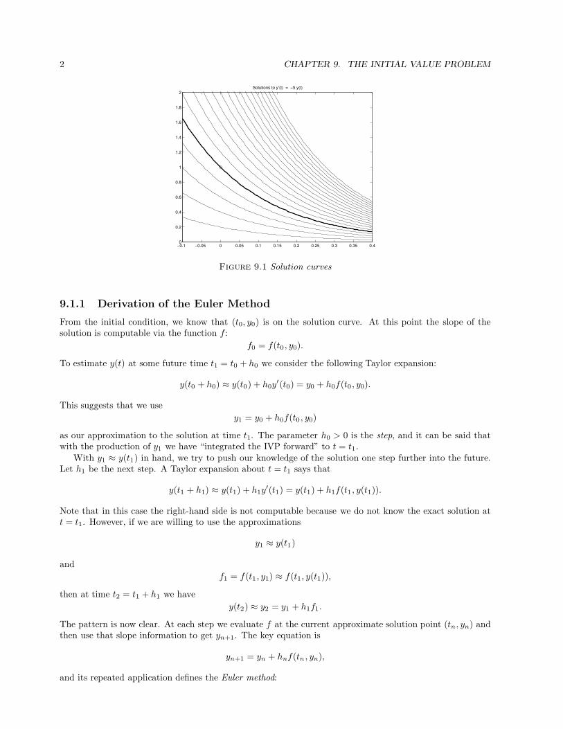
The script file ShowEuler solicits the time steps interactively and applies the Euler method to the problemy′ = −5y, y(0) = 1. (See Figure 9.2.) The determination of the step size is crucial.

−0.1 −0.05 0 0.05 0.1 0.15 0.2 0.25 0.3 0.35 0.40

0.2

0.4

0.6

0.8

1

1.2

1.4

1.6

1.8

2Five Steps of Euler Method (y’=−5y, y(0)=1)

Figure 9.2 Five steps of Euler’s method

Our intuition says that we can control error by choosing hn appropriately. Accuracy should increasewith shorter steps. On the other hand, shorter steps mean more f-evaluations as we integrate across theinterval of interest. As in the quadrature problem and the nonlinear equation-solving problem, the numberof f-evaluations usually determines execution time, and the efficiency analysis of any IVP method mustinclude a tabulation of this statistic. The basic game to be played is to get the required snapshots of y(t)with sufficient accuracy, evaluating f(t, y) as infrequently as possible. To see what we are up against, weneed to understand how the errors in the local model compound as we integrate across the time interval ofinterest.

9.1.2 Local Error, Global Error, and Stability

Assume in the Euler method that yn−1 is exact and let h = hn−1. By subtracting yn = yn−1 + hfn−1 fromthe Taylor expansion

y(tn) = yn−1 + hy′(tn−1) +h2

2y(2)(η), η ∈ [tn−1, tn],

we find that

y(tn) − yn =h2

2y(2)(η).

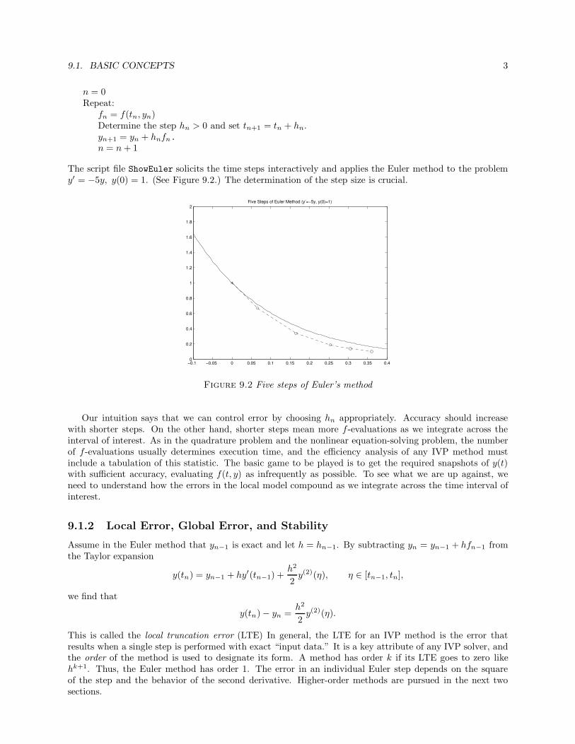
This is called the local truncation error (LTE) In general, the LTE for an IVP method is the error thatresults when a single step is performed with exact “input data.” It is a key attribute of any IVP solver, andthe order of the method is used to designate its form. A method has order k if its LTE goes to zero likehk+1. Thus, the Euler method has order 1. The error in an individual Euler step depends on the squareof the step and the behavior of the second derivative. Higher-order methods are pursued in the next twosections.


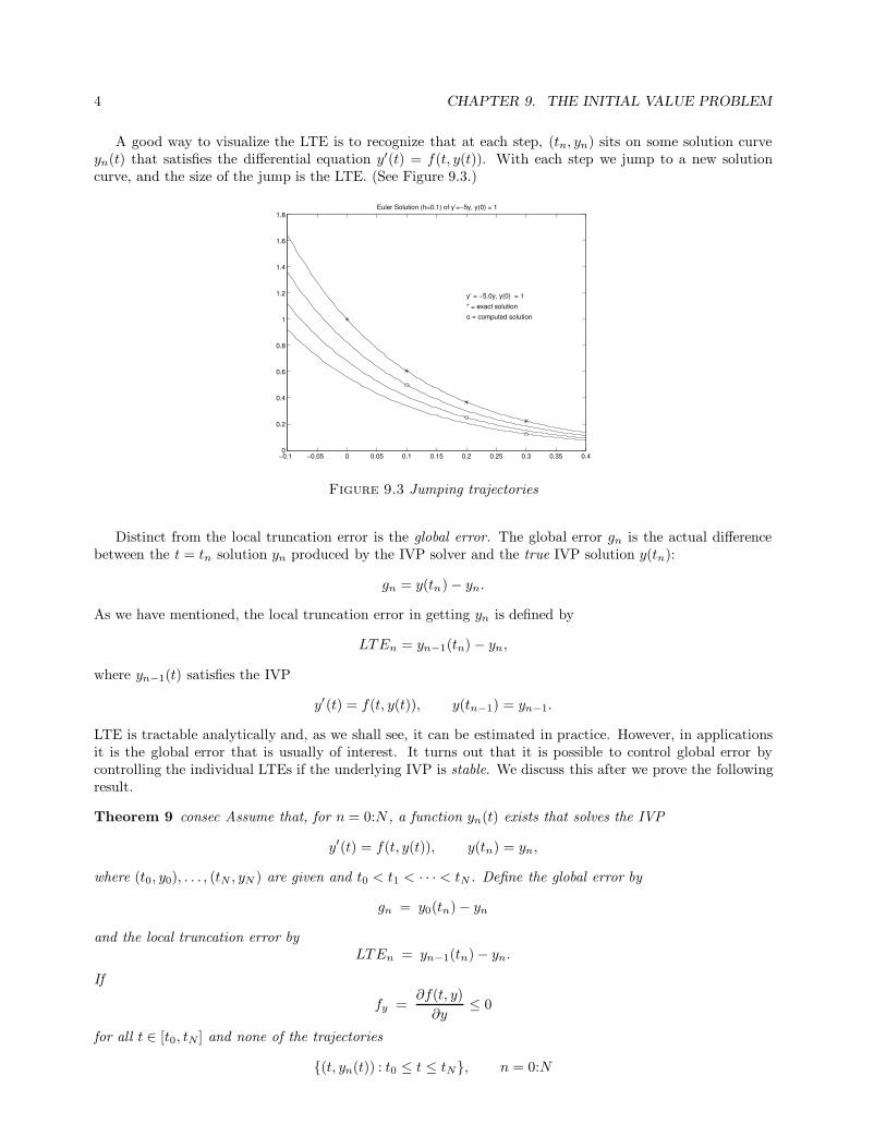
A good way to visualize the LTE is to recognize that at each step, (tn, yn) sits on some solution curveyn(t) that satisfies the differential equation y′(t) = f(t, y(t)). With each step we jump to a new solutioncurve, and the size of the jump is the LTE. (See Figure 9.3.)

−0.1 −0.05 0 0.05 0.1 0.15 0.2 0.25 0.3 0.35 0.40

0.2

0.4

0.6

0.8

1

1.2

1.4

1.6

1.8

y’ = −5.0y, y(0) = 1

* = exact solution

o = computed solution

Euler Solution (h=0.1) of y’=−5y, y(0) = 1

Figure 9.3 Jumping trajectories

Distinct from the local truncation error is the global error. The global error gn is the actual differencebetween the t = tn solution yn produced by the IVP solver and the true IVP solution y(tn):

gn = y(tn) − yn.

As we have mentioned, the local truncation error in getting yn is defined by

LTEn = yn−1(tn) − yn,

where yn−1(t) satisfies the IVP

y′(t) = f(t, y(t)), y(tn−1) = yn−1.

LTE is tractable analytically and, as we shall see, it can be estimated in practice. However, in applicationsit is the global error that is usually of interest. It turns out that it is possible to control global error bycontrolling the individual LTEs if the underlying IVP is stable. We discuss this after we prove the followingresult.

Theorem 9 consec Assume that, for n = 0:N , a function yn(t) exists that solves the IVP

y′(t) = f(t, y(t)), y(tn) = yn,

where (t0, y0), . . . , (tN , yN ) are given and t0 < t1 < · · · < tN . Define the global error by

gn = y0(tn) − yn

and the local truncation error by

LTEn = yn−1(tn) − yn.

If

fy =∂f(t, y)

∂y≤ 0

for all t ∈ [t0, tN ] and none of the trajectories

{(t, yn(t)) : t0 ≤ t ≤ tN}, n = 0:N


intersect, then for n = 1:N

|gn| ≤

n∑

k=1

|LTEk|.

Proof If y0(tn) > yn−1(tn), then because fy is negative we have

∫ tn

tn−1

(f(t, y0(t)) − f(t, yn−1(t)) dt < 0.

It follows that

0 < y0(tn) − yn−1(tn) = (y0(tn−1) − yn−1(tn−1)) +

∫ tn

tn−1

(f(t, y0(t)) − f(t, yn−1(t)) dt

< (y0(tn−1) − yn−1(tn−1)) ,

and so|y0(tn) − yn−1(tn)| ≤ |y0(tn−1) − yn−1(tn−1)|. (9.1)

Likewise, if y0(tn) < yn−1(tn), then

∫ tn

tn−1

(f(t, yn−1(t)) − f(t, y0(t)) dt < 0,

and so

0 < yn−1(tn) − y0(tn) = (yn−1(tn−1) − y0(tn−1)) +

∫ tn

tn−1

(f(t, yn−1(t)) − f(t, y0(t)) dt

< yn−1(tn−1) − y0(tn−1).

Thus, in either case (9.1) holds and so

|gn| = |y0(tn) − yn|

≤ |y0(tn) − yn−1(tn)| + |yn−1(tn) − yn|

< |y0(tn−1) − yn−1(tn−1)| + |yn−1(tn) − yn|

= |gn−1| + |LTEn|.

The theorem follows by induction since g1 = LTE1. �

The theorem essentially says that if ∂f/∂y is negative across the interval of interest, then global error att = tn is less than the sum of the local errors made by the IVP solver in reaching tn. The sign of this partialderivative is tied up with the stability of the IVP. Roughly speaking, if small changes in the initial valueinduce correspondingly small changes in the IVP solution, then we say that the IVP is stable. The concept ismuch more involved than the condition/stability issues that we talked about in connection with the Ax = bproblem. The mathematics is deep and interesting but beyond what we can do here.

So instead we look at the model problem y′(t) = ay(t), y(0) = c and deduce some of the key ideas. Inthis example, ∂f/∂y = a and so Theorem 9 applies if a < 0. We know that the solution y(t) = ceat decaysif and only if a is negative. If y(t) solves the same differential equation with initial value y(0) = c, then

|y(t) − y(t)| = |c − c|eat,

showing how “earlier error” is damped out as t increases.To illustrate how global error might be controlled in practice, consider the problem of computing y(tmax)

to within a tolerance tol, where y(t) solves a stable IVP y′(t) = f(t, y(t)), y(t0) = y0. Assume that a


fixed-step Euler method is to be used and that we have a bound M2 for |y(2)(t)| on the interval [t0, tmax]. Ifh = (tmax − t0)/N is the step size, then from what we know about the local truncation error of the method,

|LTEn| ≤ M2h2

2.

Assuming that Theorem 9 applies,

|y(tmax) − yN | ≤

N∑

n=1

|LTEn| = M2Nh2

2=

tmax − t02

M2h.

Thus, to make this upper bound less than a prescribed tol > 0, we merely set N to be the smallest integerthat satisfies

(tmax − t0)2

2NM2 ≤ tol.

Here is an implementation of the overall process:

function [tvals,yvals] = FixedEuler(f,y0,t0,tmax,M2,tol)

% Fixed step Euler method.

%

% f is a handle that references a function of the form f(t,y).

% M2 a bound on the second derivative of the solution to

% y’ = f(t,y), y(t0) = y0

% on the interval [t0,tmax].

% Determine positive n so that if tvals = linspace(t0,tmax,n), then

% y(i) is within tol of the true solution y(tvals(i)) for i=1:n.

n = ceil(((tmax-t0)^2*M2)/(2*tol))+1;

h = (tmax-t0)/(n-1);

yvals = zeros(n,1);

tvals = linspace(t0,tmax,n)’;

yvals(1) = y0;

for k=1:n-1

fval = f(tvals(k),yvals(k));

yvals(k+1) = yvals(k)+h*fval;

end

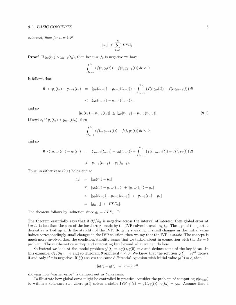
Figure 9.4 shows the error when this solution framework is applied to the model problem y′ = −y across theinterval [0, 5]. The trouble with this approach to global error control is that (1) we rarely have good boundinformation about |y(2)| and (2) it would be better to determine h adaptively so that longer step sizes canbe taken in regions where the solution is smooth. This matter is pursued in §9.3.5.

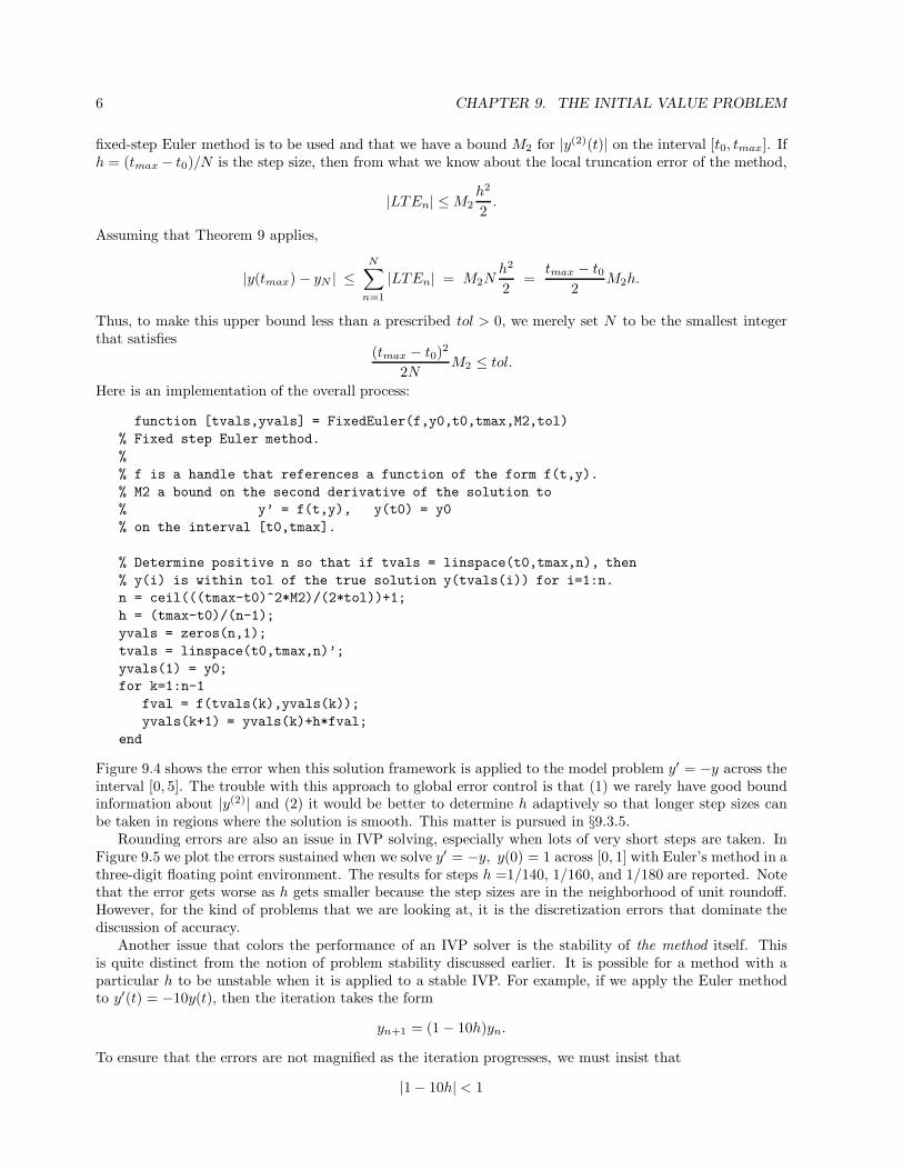
Rounding errors are also an issue in IVP solving, especially when lots of very short steps are taken. InFigure 9.5 we plot the errors sustained when we solve y′ = −y, y(0) = 1 across [0, 1] with Euler’s method in athree-digit floating point environment. The results for steps h =1/140, 1/160, and 1/180 are reported. Notethat the error gets worse as h gets smaller because the step sizes are in the neighborhood of unit roundoff.However, for the kind of problems that we are looking at, it is the discretization errors that dominate thediscussion of accuracy.

Another issue that colors the performance of an IVP solver is the stability of the method itself. Thisis quite distinct from the notion of problem stability discussed earlier. It is possible for a method with aparticular h to be unstable when it is applied to a stable IVP. For example, if we apply the Euler methodto y′(t) = −10y(t), then the iteration takes the form

yn+1 = (1 − 10h)yn.

To ensure that the errors are not magnified as the iteration progresses, we must insist that

|1− 10h| < 1


0 0.5 1 1.5 2 2.5 3 3.5 4 4.5 50

1

2

3

4

5

6

7

8x 10

−4 Fixed h Euler Error for y’=−y, y(0) = 1

tol = 0.010, n = 1251

Figure 9.4 Error in fixed-step Euler

0 0.1 0.2 0.3 0.4 0.5 0.6 0.7 0.8 0.9 10

0.005

0.01

0.015

0.02

0.025

0.03

0.035

0.04

0.045

0.05Euler in 3−Digit Arithmetic

n = 140

n = 160

n = 180

Err

or

Figure 9.5 Roundoff error in fixed-step Euler

(i.e., h < 1/5). For all h that satisfy this criterion, the method is stable. If h > 1/5, then any error δ inthe initial condition will result in a (1 − 10h)nδ contamination of the nth iterate. With this kind of errormagnification, we say that the method is unstable. Different methods have different h restrictions in order toguarantee stability, and sometimes these restrictions force us to choose h much smaller than we would like.

9.1.3 The Backward Euler Method

To clarify this point about method stability, we examine the backward Euler method. The (forward) Eulermethod is derived from a Taylor expansion of the solution y(t) about t = tn. If instead we work with theapproximation

y(tn+1 + h) ≈ y(tn+1) + y′(tn+1)h = y(tn+1) + f(tn+1 , y(tn+1))h

and set h = −hn = (tn − tn+1), then we get

y(tn) ≈ y(tn+1) − hnf(tn+1, y(tn+1)).

Substituting yn for y(tn) and yn+1 for y(tn+1), we are led to


yn+1 = yn + hnf(tn+1 , yn+1)

and, with repetition, the backward Euler framework:

n = 0Repeat:

Determine the step hn > 0.tn+1 = tn + hn.

Let yn+1 solve F (z) = z − hnf(tn+1 , z) − yn = 0.n = n + 1

Like the Euler method, the backward Euler method is first order. However, the two techniques differ in avery important aspect. Backward Euler is an implicit method because it defines yn+1 implicitly. For a simpleproblem like y′ = ay this poses no difficulty:

yn+1 = yn + hnayn+1 =1

1 − hnayn.

Observe that if a < 0, then the method is stable for all choices of positive step size. This should be contrastedwith the situation in the Euler setting, where |1 + ah| < 1 is required for stability.

Euler’s is an example of an explicit method, because yn+1 is defined explicity in terms of quantities alreadycomputed. [e.g., yn, f(tn , yn)]. Implicit methods tend to have better stability properties than their explicitcounterparts. But there is an implementation penalty to be paid, because yn+1 is defined as a zero of anonlinear function. In backward Euler, yn+1 is a zero of F (z) = z − hnf(tn+1, z). Fortunately, this doesnot necessarily require the application of the Chapter 8 root finders. A simpler, more effective approach ispresented in §9.3.

9.1.4 Systems

We complete the discussion of IVP solving basics with comments about systems of differential equations. Inthis case the unknown function y(t) is a vector of unknown functions:

y(t) =

z1(t)...

zd(t)

.

(We name the component functions with a z instead of a y to avoid confusion with earlier notation.) Inthis case, we are given an initial value for each component function and a recipe for its slope. This recipegenerally involves the value of all the component functions:

z′1(t)...

z′d(t)

=

f1(t, z1(t), . . . , zd(t))...

fm(t, z1(t), . . . , zd(t))

z1(t0) = z10

...zd(t0) = zd0

.

In vector language, y′(t) = f(t, y(t)), y(t0) = y0, where the y’s are now column d-vectors. Here is a d = 2example:

u′(t) = 2u(t) − .01u(t)v(t)v′(t) = −v(t) + .01u(t)v(t)

, u(0) = u0, v(0) = v0.

It describes the density of rabbit and fox populations in a classical predator-prey model. The rate of changeof the rabbit density u(t) and the fox density v(t) depend on the current rabbit/fox densities.

Let’s see how the derivation of Euler’s method proceeds for a systems problem like this. We start witha pair of time-honored Taylor expansions:

u(tn+1) ≈ u(tn) + u′(tn)hn = u(tn) + hn(2u(tn) − .01u(tn)v(tn))

v(tn+1) ≈ v(tn) + v′(tn)hn = v(tn) + hn(−v(tn) + .01u(tn)v(tn))


Here (as usual), tn+1 = tn + hn. With the definitions

yn =

[

un

vn

]

≈

[

u(tn)v(tn)

]

= y(tn)

and

fn = f(tn , yn) =

[

2un − .01unvn

−vn + .01unvn

]

≈

[

2u(tn) − .01u(tn)v(tn)−v(tn) + .01u(tn)v(tn)

]

= f(tn, y(tn)),

we obtain he following vector implementation of the Euler method:[

un+1

vn+1

]

=

[

un

vn

]

+ hn

[

2un − .01unvn

−vn + .01unvn

]

.

In full vector notation, this can be written as

yn+1 = yn + hnfn,

which is exactly the same formula that we developed in the scalar case.As we go through the next two sections presenting more sophisticated IVP solvers, we shall do so for

scalar (d = 1) problems, being mindful that all method-defining equations apply at the system level with nomodification.

Systems can arise in practice from the conversion of higher-order IVPs. In a kth order IVP, we seek afunction y(t) that satisfies

y(k)(t) = f(t, y(t), y(1)(t), . . . , y(k−1)(t)) where

y(t0) = y0

y(1)(t0) = y(1)0

...

y(k−1)(t0) = y(k−1)0

and y0, y(1)0 , . . . , y

(k−1)0 are given initial values. Higher order IVPs can be solved through conversion to a

system of first-order IVPs. For example, to solve

v′′(t) = 2v(t) + v′(t) sin(t), v(0) = α, v′(0) = β,

we define z1(t) = v(t) and z2(t) = v′(t). The problem then transforms to

z′1(t) = z2(t)z′2(t) = 2z1(t) + z2(t) sin(t)

, z1(0) = α, z2(0) = β.

Problems

P9.1.1 Produce a plot of the solution to

y′(t) = −ty +1

y2, y(1) = 1

across the interval [1,2]. Use the Euler method.

P9.1.2 Compute an approximation to y(1) where

x′′(t) = (3 − sin(t))x′(t) + x(t)/(1 + [y(t)]2),

y′(t) = − cos(t)y(t) − x′(t)/(1 + t2),

x(0) = 3, x′(0) = −1, and y(0) = 4. Use the forward Euler method with fixed step determined so that three significant digits ofaccuracy are obtained. Hint: Define z(t) = x′(t) and rewrite the recipe for x′′ as a function of x, y, and z. This yields a d = 3system.

P9.1.3 Plot the solutions to

y′(t) =

»

−1 4−4 −1

–

y(t), y(0) =

»

2−1

–

across the interval [0,3].

P9.1.4 Consider the initial value problemAy′(t) = By(t), y(0) = y0,

where A and B are given n-by-n matrices with A nonsingular. For fixed step size h, explain how the backwards Euler methodcan be used to compute approximate solutions at t = kh, k = 1:100.


9.2 The Runge-Kutta Methods

In an Euler step, we “extrapolate into the future” with only a single sampling of the slope function f(t, y).The method has order 1 because its LTE goes to zero as h2. Just as we moved beyond the trapezoidalrule in Chapter 4, so we must now move beyond the Euler framework with more involved models of theslope function. In the Runge-Kutta framework, we sample f at several judiciously chosen spots and use theinformation to obtain yn+1 from yn with the highest possible order of accuracy.

9.2.1 Derivation

The Euler methods evaluate f once per step and have order 1. Let’s sample f twice per step and see if wecan obtain a second-order method. We arrange it so that the second evaluation depends on the first:

k1 = hf(tn , yn)

k2 = hf(tn + αh, yn + βk1)

yn+1 = yn + ak1 + bk2 .

Our goal is to choose the parameters α, β, a, and b so that the LTE is O(h3). From the Taylor series wehave

y(tn+1) = y(tn) + y(1)(tn)h + y(2)(tn)h2

2+ O(h3).

Since

y(1)(tn) = f

y(2)(tn) = ft + fyf

where

f = f(tn , yn)

ft =∂f(tn , yn)

∂t

fy =∂f(tn , yn)

∂y,

it follows that

y(tn+1) = y(tn) + fh + (ft + fyf)h2

2+ O(h3). (9.2)

On the other hand,

k2 = hf(tn + αh, yn + βk1) = h(

f + αhft + βk1fy + O(h2))

and so

yn+1 = yn + ak1 + bk2 = yn + (a + b) fh + b (αft + βffy )h2 + O(h3). (9.3)

For the LTE to be O(h3), the equation

y(tn+1) − yn+1 = O(h3)

must hold. To accomplish this, we compare terms in (9.2) and (9.3) and require

a + b = 1

2bα = 1

2bβ = 1 .

9.2. THE RUNGE-KUTTA METHODS 11

There are an infinite number of solutions to this system, the canonical one being a = b = 1/2 and α = β = 1.With this choice the LTE is O(h3), and we obtain a second-order Runge-Kutta method:

k1 = hf(tn , yn)

k2 = hf(tn + h, yn + k1)

yn+1 = yn + (k1 + k2)/2 .

The actual expression for the LTE is given by

LTE(RK2) =h3

12(ftt + 2ffty + f2fyy − 2ftfy − 2ff2

y ),

where the partials on the right are evaluated at some point in [tn, tn + h]. Notice that two f-evaluations arerequired per step.

The most famous Runge-Kutta method is the classical fourth order method:

k1 = hf(tn , yn)

k2 = hf(tn + h2 , yn + 1

2k1)

k3 = hf(tn + h2 , yn + 1

2k2)

k4 = hf(tn + h, yn + k3)

yn+1 = yn + 16(k1 + 2k2 + 2k3 + k4) .

This can be derived using the same Taylor expansion technique illustrated previously. It requires fourf-evaluations per step.

The function RKStep can be used to carry out a Runge-Kutta step of prescribed order. Here is itsspecification along with an abbreviated portion of the implementation:

function [tnew,ynew,fnew] = RKstep(f,tc,yc,fc,h,k)

% f is a handle that references a function of the form f(t,y)

% where t is a scalar and y is a column d-vector.

% yc is an approximate solution to y’(t) = f(t,y(t)) at t=tc.

% fc = f(tc,yc).

% h is the time step.

% k is the order of the Runge-Kutta method used, 1<=k<=5.

% tnew=tc+h, ynew is an approximate solution at t=tnew, and

% fnew = f(tnew,ynew).

if k==1

k1 = h*fc;

ynew = yc + k1;

elseif k==2

k1 = h*fc;

k2 = h*f(tc+(h),yc+(k1));

ynew = yc + (k1 + k2)/2;

elseif k==3

k1 = h*fc;

k2 = h*f(tc+(h/2),yc+(k1/2));

k3 = h*f(tc+h,yc-k1+2*k2);

ynew = yc + (k1 + 4*k2 + k3)/6;

elseif k==4

:

end

tnew = tc+h;

fnew = f(tnew,ynew);


As can be imagined, symbolic algebra tools are useful in the derivation of such an involved sampling andcombination of f-values.

Problems

P9.2.1 The RKF45 method produces both a fourth order estimate and a fifth order estimate using six function evaluations:

k1 = hf(tn, yn)

k2 = hf(tn + h4, yn + 1

4k1)

k3 = hf(tn + 3h8

, yn + 332

k1 + 932

k2)

k4 = hf(tn + 12h13

, yn + 19322197

k1 − 72002197

k2 + 72962197

k3)

k5 = hf(tn + h, yn + 439216

k1 − 8k2 + 3680513

k3 − 8454104

k4)

k6 = hf(tn + h2, yn − 8

27k1 + 2k2 − 3544

2565k3 + 1859

4104k4 − 11

40k5)

yn+1 = yn + 25216

k1 + 14082565

k3 + 21974104

k4 − 15k5

zn+1 = yn + 16135

k1 + 665612825

k3 + 2856156430

k4 − 950

k5 + 255

k6 .

Write a script that discovers which of yn+1 and zn+1 is the fourth order estimate and which is the fifth order estimate.

9.2.2 Implementation

Runge-Kutta steps can obviously be repeated, and if we keep the step size fixed, then we obtain the followingimplementation:

function [tvals,yvals] = FixedRK(f,t0,y0,h,k,n)

% [tvals,yvals] = FixedRK(fname,t0,y0,h,k,n)

% Produces approximate solution to the initial value problem

%

% y’(t) = f(t,y(t)) y(t0) = y0

%

% using a strategy that is based upon a k-th order Runge-Kutta method. Stepsize

% is fixed. f is a handle that references the function f, t0 is the initial time,

% y0 is the initial condition vector, h is the stepsize, k is the order of

% method (1<=k<=5), and n is the number of steps to be taken,

% tvals(j) = t0 + (j-1)h, j=1:n+1

% yvals(j,:) = approximate solution at t = tvals(j), j=1:n+1

tc = t0; tvals = tc;

yc = y0; yvals = yc’;

fc = f(tc,yc);

for j=1:n

[tc,yc,fc] = RKstep(f,tc,yc,fc,h,k);

yvals = [yvals; yc’];

tvals = [tvals tc];

end

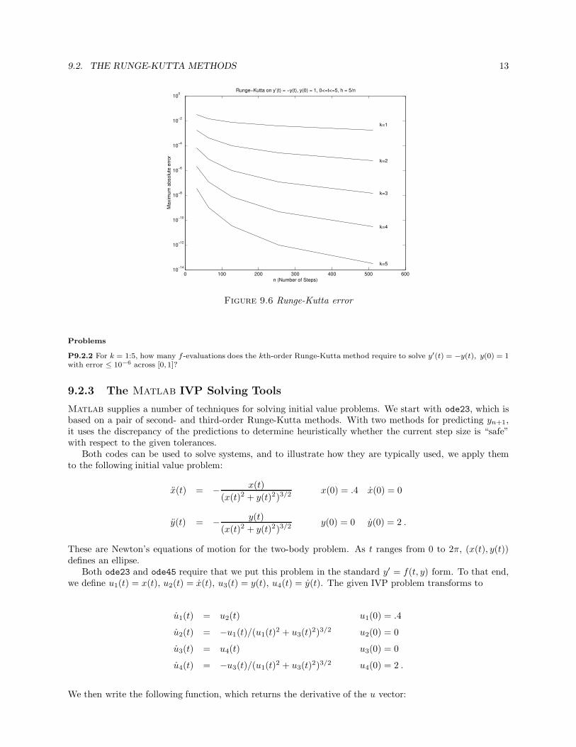
The function file ShowRK can be used to illustrate the performance of the Runge-Kutta methods on theIVP y′ = −y, y(0) = 1. The results are reported in Figure 9.6. All the derivatives of f are “nice,” whichmeans that if we increase the order and keep the step size fixed, then the errors should diminish by a factorof h. Thus for n = 500, h = 1/100 and we find that the error in the kth order method is about 100−k.

Do not conclude from the example that higher-order methods are necessarily more accurate. If the higherderivatives of the solution are badly behaved, then it may well be the case that a lower-order method givesmore accurate results. One must also be mindful of the number of f-evaluations that are required to purchasea given level of accuracy. The situation is analogous to what we found in the quadrature unit. Of course,the best situation is for the IVP software to handle the selection of method and step.


0 100 200 300 400 500 60010

−14

10−12

10−10

10−8

10−6

10−4

10−2

100

Runge−Kutta on y’(t) = −y(t), y(0) = 1, 0<=t<=5, h = 5/n

n (Number of Steps)

Maxim

um

absolu

te e

rror

k=1

k=2

k=3

k=4

k=5

Figure 9.6 Runge-Kutta error

Problems

P9.2.2 For k = 1:5, how many f -evaluations does the kth-order Runge-Kutta method require to solve y′(t) = −y(t), y(0) = 1with error ≤ 10−6 across [0,1]?

9.2.3 The Matlab IVP Solving Tools

Matlab supplies a number of techniques for solving initial value problems. We start with ode23, which isbased on a pair of second- and third-order Runge-Kutta methods. With two methods for predicting yn+1,it uses the discrepancy of the predictions to determine heuristically whether the current step size is “safe”with respect to the given tolerances.

Both codes can be used to solve systems, and to illustrate how they are typically used, we apply themto the following initial value problem:

x(t) = −x(t)

(x(t)2 + y(t)2)3/2 x(0) = .4 x(0) = 0

y(t) = −y(t)

(x(t)2 + y(t)2)3/2 y(0) = 0 y(0) = 2 .

These are Newton’s equations of motion for the two-body problem. As t ranges from 0 to 2π, (x(t), y(t))defines an ellipse.

Both ode23 and ode45 require that we put this problem in the standard y′ = f(t, y) form. To that end,we define u1(t) = x(t), u2(t) = x(t), u3(t) = y(t), u4(t) = y(t). The given IVP problem transforms to

u1(t) = u2(t) u1(0) = .4

u2(t) = −u1(t)/(u1(t)2 + u3(t)

2)3/2 u2(0) = 0

u3(t) = u4(t) u3(0) = 0

u4(t) = −u3(t)/(u1(t)2 + u3(t)

2)3/2 u4(0) = 2 .

We then write the following function, which returns the derivative of the u vector:


function up = Kepler(t,u)

% up = Kepler(t,u)

% t (time) is a scalar and u is a 4-vector whose components satisfy

%

% u(1) = x(t) u(2) = (d/dt)x(t)

% u(3) = y(t) u(4) = (d/dt)y(t)

%

% where (x(t),y(t)) are the equations of motion in the 2-body problem.

%

% up is a 4-vector that is the derivative of u at time t.

r3 = (u(1)^2 + u(3)^2)^1.5;

up = [ u(2) ;...

-u(1)/r3 ;...

u(4) ;...

-u(3)/r3] ;

With this function available, we can call ode23 and plot various results:

tInitial = 0;

tFinal = 2*pi;

uInitial = [ .4; 0 ; 0 ; 2];

tSpan = [tInitial tFinal];

[t, u] = ode23(@Kepler, tSpan, uInitial);

ode23 requires that we pass the name of the “slope function”, the span of integration, and the initialcondition vector. The slope function must be of the form f(t,y) where t is a scalar and y is a vector. Itmust return a column vector. In this call the tSpan vector simply specifies the initial and final times. Theoutput produced is a column vector of times t and a matrix u of solution snapshots. If n = length(t) then(a) t(0) = tInitial, t(n) = tFinal, and u(k,:) is an approximation to the solution at time t(k). Thetime step lengths and (therefore their number) is determined by the default error tolerance: Reltol = 10−3

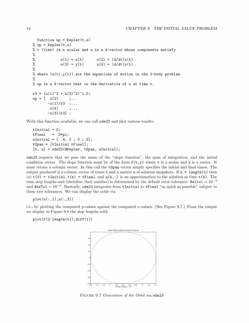
and AbsTol = 10−6. Basically, ode23 integrates from tInitial to tFinal “as quick as possible” subject tothese two tolerances. We can display the orbit via

plot(u(:,1),u(:,3))

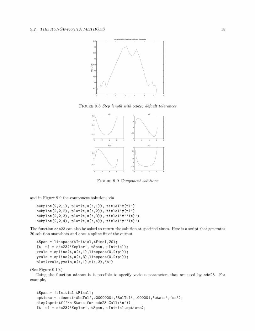
i.e., by plotting the computed y-values against the computed x-values. (See Figure 9.7.) From the outputwe display in Figure 9.8 the step lengths with

plot(t(2:length(t)),diff(t))

−1.6 −1.4 −1.2 −1 −0.8 −0.6 −0.4 −0.2 0 0.2 0.4−0.8

−0.6

−0.4

−0.2

0

0.2

0.4

0.6

Kepler Problem: ode23 with Default Tolerances

Number of Steps = 53

Figure 9.7 Generation of the Orbit via ode23


0 1 2 3 4 5 6 70

0.05

0.1

0.15

0.2

0.25

0.3

0.35

0.4

0.45Kepler Problem: ode23 with Default Tolerances

Ste

p L

ength

t

Figure 9.8 Step length with ode23 default tolerances

0 2 4 6 8−2

−1.5

−1

−0.5

0

0.5x(t)

0 2 4 6 8−1

−0.5

0

0.5

1y(t)

0 2 4 6 8−1

−0.5

0

0.5

1x’(t)

0 2 4 6 8−1

−0.5

0

0.5

1

1.5

2y’(t)

Figure 9.9 Component solutions

and in Figure 9.9 the component solutions via

subplot(2,2,1), plot(t,u(:,1)), title(’x(t)’)

subplot(2,2,2), plot(t,u(:,2)), title(’y(t)’)

subplot(2,2,3), plot(t,u(:,3)), title(’x’’(t)’)

subplot(2,2,4), plot(t,u(:,4)), title(’y’’(t)’)

The function ode23 can also be asked to return the solution at specified times. Here is a script that generates20 solution snapshots and does a spline fit of the output

tSpan = linspace(tInitial,tFinal,20);

[t, u] = ode23(’Kepler’, tSpan, uInitial);

xvals = spline(t,u(:,1),linspace(0,2*pi));

yvals = spline(t,u(:,3),linspace(0,2*pi));

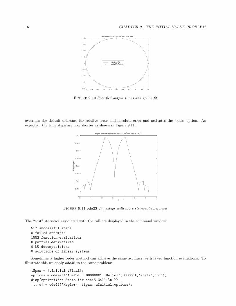
plot(xvals,yvals,u(:,1),u(:,3),’o’)

(See Figure 9.10.)Using the function odeset it is possible to specify various parameters that are used by ode23. For

example,


options = odeset(’AbsTol’,.00000001,’RelTol’,.000001,’stats’,’on’);

disp(sprintf(’\n Stats for ode23 Call:\n’))

[t, u] = ode23(’Kepler’, tSpan, uInitial,options);


−1.6 −1.4 −1.2 −1 −0.8 −0.6 −0.4 −0.2 0 0.2 0.4−0.8

−0.6

−0.4

−0.2

0

0.2

0.4

0.6

0.8Kepler Problem: ode23 with Specified Output Times

Spline Fitode23 Output

Figure 9.10 Specified output times and spline fit

overrides the default tolerance for relative error and absolute error and activates the ’stats’ option. Asexpected, the time steps are now shorter as shown in Figure 9.11.

0 1 2 3 4 5 6 70

0.005

0.01

0.015

0.02

0.025

0.03

0.035

0.04Kepler Problem: ode23 with RelTol = 10

−6 and AbsTol = 10

−8

Ste

p L

en

gth

t

Figure 9.11 ode23 Timesteps with more stringent tolerances

The “cost” statistics associated with the call are displayed in the command window:

517 successful steps

0 failed attempts

1552 function evaluations

0 partial derivatives

0 LU decompositions

0 solutions of linear systems

Sometimes a higher order method can achieve the same accuracy with fewer function evaluations. Toillustrate this we apply ode45 to the same problem:


options = odeset(’AbsTol’,.00000001,’RelTol’,.000001,’stats’,’on’);

disp(sprintf(’\n Stats for ode45 Call:\n’))

[t, u] = ode45(’Kepler’, tSpan, uInitial,options);


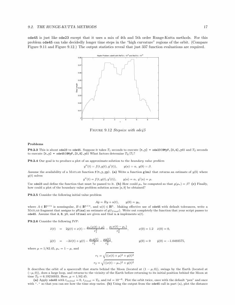
ode45 is just like ode23 except that it uses a mix of 4th and 5th order Runge-Kutta methods. For thisproblem ode45 can take decidedly longer time steps in the “high curvature” regions of the orbit. (CompareFigure 9.11 and Figure 9.12.) The output statistics reveal that just 337 function evaluations are required.

0 1 2 3 4 5 6 70

0.01

0.02

0.03

0.04

0.05

0.06

0.07

0.08Kepler Problem: ode45 with RelTol = 10

−6 and AbsTol = 10

−8

Ste

p L

en

gth

t

Figure 9.12 Stepsize with ode45

Problems

P9.2.3 This is about ode23 vs ode45. Suppose it takes T1 seconds to execute [t,y] = ode23(@MyF,[0,4],y0) and T2 secondsto execute [t,y] = ode45(@MyF,[0,8],y0) What factors determine T2/T1?

P9.2.4 Our goal is to produce a plot of an approximate solution to the boundary value problem

y′′(t) = f(t,y(t), y′(t)), y(a) = α, y(b) = β.

Assume the availability of a Matlab function f(t,y,yp). (a) Write a function g(mu) that returns an estimate of y(b) wherey(t) solves

y′′(t) = f(t, y(t), y′(t)), y(a) = α, y′(a) = µ.

Use ode23 and define the function that must be passed to it. (b) How could µ∗ be computed so that g(µ∗) = β? (c) Finally,how could a plot of the boundary value problem solution across [a, b] be obtained?

P9.2.5 Consider the following initial value problem

Ay = By + u(t), y(0) = y0,

where A ∈ IRn×n is nonsingular, B ∈ IRn×n, and u(t) ∈ IRn. Making effective use of ode45 with default tolerances, write aMatlab fragment that assigns to yFinal an estimate of y(tfinal). Write out completely the function that your script passes toode45. Assume that A, B, y0, and tfinal are given and that u.m implements u(t).

P9.2.6 Consider the following IVP:

x(t) = 2y(t) + x(t) −µ∗(x(t) + µ)

r31

−µ(x(t) − µ∗)

r32

, x(0) = 1.2 x(0) = 0,

y(t) = −2x(t) + y(t) −µ∗y(t)

r31

−µy(t)

r32

, y(0) = 0 y(0) = −1.0493575,

where µ = 1/82.45, µ∗ = 1 − µ, and

r1 =q

((x(t) + µ)2 + y(t)2

r2 =q

((x(t) − µ∗)2 + y(t)2

It describes the orbit of a spacecraft that starts behind the Moon (located at (1 − µ, 0)), swings by the Earth (located at(−µ, 0)), does a large loop, and returns to the vicinity of the Earth before returning to its initial position behind the Moon attime T0 = 6.19216933. Here, µ = 1/82.45.

(a) Apply ode45 with tinitial = 0, tfinal = T0, and tol = 10−6. Plot the orbit twice, once with the default “pen” and oncewith ’.’ so that you can see how the time step varies. (b) Using the output from the ode45 call in part (a), plot the distance


of the spacecraft to Earth as a function of time across [0, T0]. Use spline to fit the distance “snapshots.” To within a mile,how close does the spacecraft get to the Earth’s surface? Assume that the Earth is a sphere of radius 4000 miles and that theEarth-Moon separation is 238,000 miles. Use fmin with an appropriate spline for the objective function. Note that the IVPis scaled so that one unit of distance is 238,000 miles. (c) Repeat Part (a) with ode23. (d) Apply ode45 with tinitial = 0,tfinal = 2T0, and tol = 10−6, but change y(0) to and y(0) = −.8. Plot the orbit. For a little more insight into what happens,repeat with tfinal = 8 ∗ T0. (e) To the nearest minute, compute how long the spacecraft is hidden to an observer on earthas it swings behind the Moon during its orbit. Assume that the observer is at (−µ, 0) and that the Moon has diameter 2160miles. Make intelligent use of fzero. (f) Find t∗ in the interval [0, T0/2] so that at time t∗, the spacecraft is equidistant fromthe Moon and the Earth.

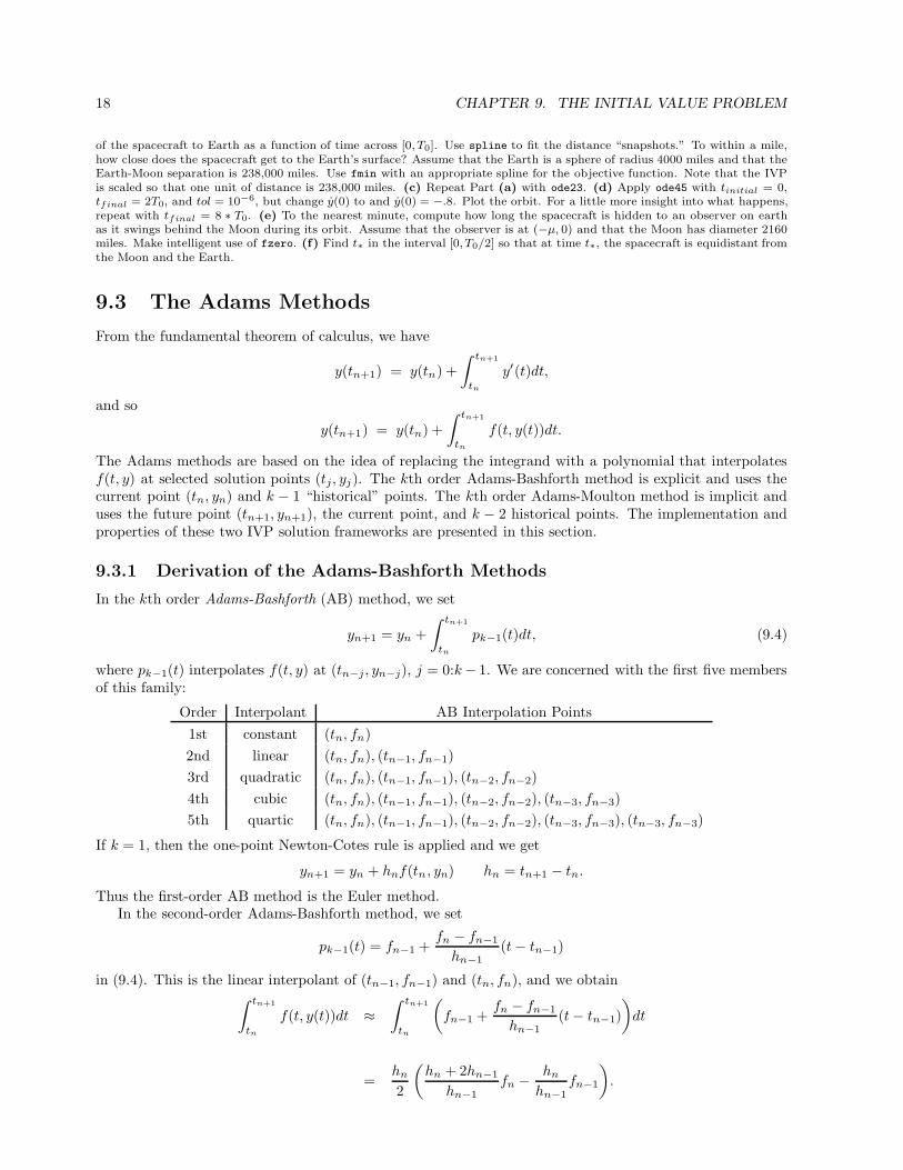
9.3 The Adams Methods

From the fundamental theorem of calculus, we have

y(tn+1) = y(tn) +

∫ tn+1

tn

y′(t)dt,

and so

y(tn+1) = y(tn) +

∫ tn+1

tn

f(t, y(t))dt.

The Adams methods are based on the idea of replacing the integrand with a polynomial that interpolatesf(t, y) at selected solution points (tj, yj). The kth order Adams-Bashforth method is explicit and uses thecurrent point (tn, yn) and k − 1 “historical” points. The kth order Adams-Moulton method is implicit anduses the future point (tn+1, yn+1), the current point, and k − 2 historical points. The implementation andproperties of these two IVP solution frameworks are presented in this section.

9.3.1 Derivation of the Adams-Bashforth Methods

In the kth order Adams-Bashforth (AB) method, we set

yn+1 = yn +

∫ tn+1

tn

pk−1(t)dt, (9.4)

where pk−1(t) interpolates f(t, y) at (tn−j, yn−j), j = 0:k− 1. We are concerned with the first five membersof this family:

Order Interpolant AB Interpolation Points

1st constant (tn, fn)

2nd linear (tn, fn), (tn−1, fn−1)

3rd quadratic (tn, fn), (tn−1, fn−1), (tn−2, fn−2)

4th cubic (tn, fn), (tn−1, fn−1), (tn−2, fn−2), (tn−3, fn−3)

5th quartic (tn, fn), (tn−1, fn−1), (tn−2, fn−2), (tn−3, fn−3), (tn−3, fn−3)

If k = 1, then the one-point Newton-Cotes rule is applied and we get

yn+1 = yn + hnf(tn , yn) hn = tn+1 − tn.

Thus the first-order AB method is the Euler method.In the second-order Adams-Bashforth method, we set

pk−1(t) = fn−1 +fn − fn−1

hn−1(t − tn−1)

in (9.4). This is the linear interpolant of (tn−1, fn−1) and (tn, fn), and we obtain∫ tn+1

tn

f(t, y(t))dt ≈

∫ tn+1

tn

(

fn−1 +fn − fn−1

hn−1(t − tn−1)

)

dt

=hn

2

(

hn + 2hn−1

hn−1fn −

hn

hn−1fn−1

)

.

9.3. THE ADAMS METHODS 19

If hn = hn−1 = h, then from (9.4)

yn+1 = yn +h

2(3fn − fn−1) .

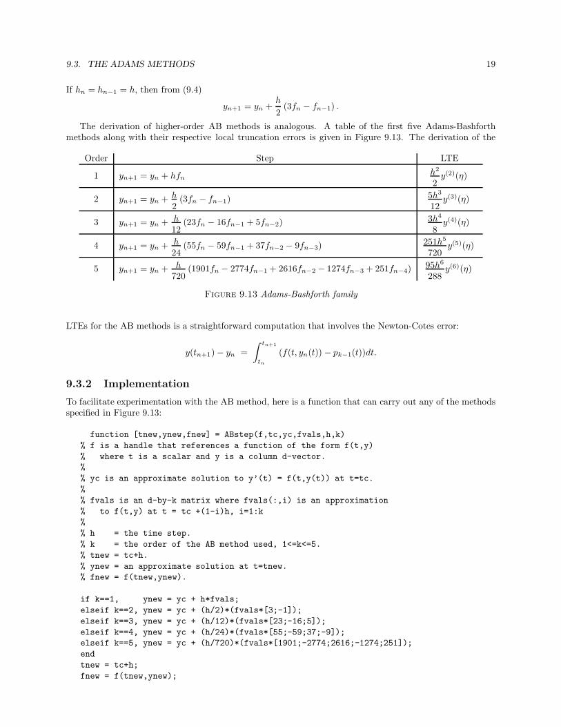
The derivation of higher-order AB methods is analogous. A table of the first five Adams-Bashforthmethods along with their respective local truncation errors is given in Figure 9.13. The derivation of the

Order Step LTE

1 yn+1 = yn + hfnh2

2y(2)(η)

2 yn+1 = yn + h2

(3fn − fn−1)5h3

12y(3)(η)

3 yn+1 = yn + h12

(23fn − 16fn−1 + 5fn−2)3h4

8y(4)(η)

4 yn+1 = yn + h24

(55fn − 59fn−1 + 37fn−2 − 9fn−3)251h5

720y(5)(η)

5 yn+1 = yn + h720

(1901fn − 2774fn−1 + 2616fn−2 − 1274fn−3 + 251fn−4)95h6

288y(6)(η)

Figure 9.13 Adams-Bashforth family

LTEs for the AB methods is a straightforward computation that involves the Newton-Cotes error:

y(tn+1) − yn =

∫ tn+1

tn

(f(t, yn(t)) − pk−1(t))dt.

9.3.2 Implementation

To facilitate experimentation with the AB method, here is a function that can carry out any of the methodsspecified in Figure 9.13:

function [tnew,ynew,fnew] = ABstep(f,tc,yc,fvals,h,k)



%


%

% fvals is an d-by-k matrix where fvals(:,i) is an approximation

% to f(t,y) at t = tc +(1-i)h, i=1:k

%

% h = the time step.

% k = the order of the AB method used, 1<=k<=5.

% tnew = tc+h.

% ynew = an approximate solution at t=tnew.


if k==1, ynew = yc + h*fvals;

elseif k==2, ynew = yc + (h/2)*(fvals*[3;-1]);

elseif k==3, ynew = yc + (h/12)*(fvals*[23;-16;5]);

elseif k==4, ynew = yc + (h/24)*(fvals*[55;-59;37;-9]);

elseif k==5, ynew = yc + (h/720)*(fvals*[1901;-2774;2616;-1274;251]);

end

tnew = tc+h;



In the systems case, fval is a matrix and ynew is yc plus a matrix-vector product.Note that k snapshots of f(t, y) are required, and this is why Adams methods are called multistep

methods. Because of this there is a “start-up” issue with the Adams-Bashforth method: How do we performthe first step when there is no “history”? There are several approaches to this, and care must be taken toensure that the accuracy of the generated start-up values is consistent with the overall accuracy aims. Fora kth order Adams framework we use a kth order Runge-Kutta method, to get fj = f(tj , yj), j = 1:k − 1.See the function ABStart. Using ABStart we are able to formulate a fixed-step Adams-Bashforth solver:

function [tvals,yvals] = FixedAB(f,t0,y0,h,k,n)

% Produces an approximate solution to the initial value problem

% y’(t) = f(t,y(t)), y(t0) = y0 using a strategy that is based upon a k-th order

% Adams-Bashforth method. Stepsize is fixed.

%

% f = handle that references the function f.

% t0 = initial time.

% y0 = initial condition vector.

% h = stepsize.

% k = order of method. (1<=k<=5).

% n = number of steps to be taken,

%

% tvals(j) = t0 + (j-1)h, j=1:n+1


[tvals,yvals,fvals] = ABStart(f,t0,y0,h,k);

tc = tvals(k);

yc = yvals(k,:)’;

fc = fvals(:,k);

for j=k:n

% Take a step and then update.

[tc,yc,fc] = ABstep(f,tc,yc,fvals,h,k);

tvals = [tvals tc];


fvals = [fc fvals(:,1:k-1)];

end

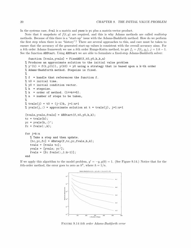
If we apply this algorithm to the model problem, y′ = −y, y(0) = 1. (See Figure 9.14.) Notice that for thekth-order method, the error goes to zero as hk, where h = 1/n.

0 100 200 300 400 500 60010

−12

10−10

10−8

10−6

10−4

10−2

Adams−Bashforth on y’(t) = −y(t), y(0) = 1, 0<=t<=5, h = 5/n

n (Number of Steps)

Maxim

um

absolu

te e

rror

k=1

k=2

k=3

k=4

k=5

Figure 9.14 kth order Adams-Bashforth error


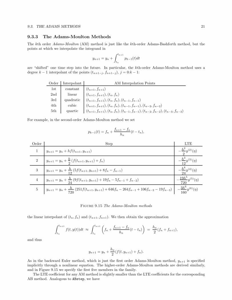
9.3.3 The Adams-Moulton Methods

The kth order Adams-Moulton (AM) method is just like the kth-order Adams-Bashforth method, but thepoints at which we interpolate the integrand in

yn+1 = yn +

∫ tn+1

tn

pk−1(t)dt

are “shifted” one time step into the future. In particular, the kth-order Adams-Moulton method uses adegree k − 1 interpolant of the points (tn+1−j , fn+1−j), j = 0:k − 1:

Order Interpolant AM Interpolation Points

1st constant (tn+1, fn+1)

2nd linear (tn+1, fn+1), (tn, fn)

3rd quadratic (tn+1, fn+1), (tn, fn), (tn−1, fn−1)

4th cubic (tn+1, fn+1), (tn, fn), (tn−1, fn−1), (tn−2, fn−2)

5th quartic (tn+1, fn+1), (tn, fn), (tn−1, fn−1), (tn−2, fn−2), (tn−3, fn−3)

For example, in the second-order Adams-Moulton method we set

pk−1(t) = fn +fn+1 − fn

hn(t − tn),

Order Step LTE

1 yn+1 = yn + hf(tn+1, yn+1) −h2

2y(2)(η)

2 yn+1 = yn + h2

(f(tn+1, yn+1) + fn) −h3

12y(3)(η)

3 yn+1 = yn + h12

(5f(tn+1, yn+1) + 8fn − fn−1) −h4

24y(4)(η)

4 yn+1 = yn + h24

(9f(tn+1, yn+1) + 19fn − 5fn−1 + fn−2) −19h5

720y(5)(η)

5 yn+1 = yn + h720

(251f(tn+1, yn+1) + 646fn − 264fn−1 + 106fn−2 − 19fn−3) −3h6

160y(6)(η)

Figure 9.15 The Adams-Moulton methods

the linear interpolant of (tn, fn) and (tn+1, fn+1). We then obtain the approximation

∫ tn+1

tn

f(t, y(t))dt ≈

∫ tn+1

tn

(

fn +fn+1 − fn

hn(t − tn)

)

=hn

2(fn + fn+1),

and thus

yn+1 = yn +hn

2(f(t, yn+1) + fn).

As in the backward Euler method, which is just the first order Adams-Moulton method, yn+1 is specifiedimplicitly through a nonlinear equation. The higher-order Adams-Moulton methods are derived similarly,and in Figure 9.15 we specify the first five members in the family.

The LTE coefficient for any AM method is slightly smaller than the LTE coefficients for the correspondingAB method. Analogous to ABstep, we have


function [tnew,ynew,fnew] = AMstep(f,tc,yc,fvals,h,k)

% Single step of the kth order Adams-Moulton method.

%



%


%

% fvals is an d-by-k matrix where fvals(:,i) is an approximation

% to f(t,y) at t = tc +(2-i)h, i=1:k.

%

% h is the time step.

%

% k is the order of the AM method used, 1<=k<=5.

%

% tnew=tc+h

% ynew is an approximate solution at t=tnew


if k==1, ynew = yc + h*fvals;

elseif k==2, ynew = yc + (h/2)*(fvals*[1;1]);

elseif k==3, ynew = yc + (h/12)*(fvals*[5;8;-1]);

elseif k==4, ynew = yc + (h/24)*(fvals*[9;19;-5;1]);

elseif k==5, ynew = yc + (h/720)*(fvals*[251;646;-264;106;-19]);

end

tnew = tc+h;


We could discuss methods for the solution of the nonlinear F (z) = 0 that defines yn+1. However, we haveother plans for the Adams-Moulton methods that circumvent this problem.

9.3.4 The Predictor-Corrector Idea

A very important framework for solving IVPs results when we couple an Adams-Bashforth method with anAdams-Moulton method of the same order. The idea is to predict yn+1 using an Adams-Bashforth methodand then to correct its value using the corresponding Adams-Moulton method. In the second-order case,AB2 gives

y(P)n+1 = yn +

h

2(3fn − fn−1),

which then is used in the right-hand side of the AM2 recipe to render

y(C)n+1 = yn +

h

2

(

f(tn+1 , y(P)n+1) + fn

)

.

For general order we have developed a function

[tnew,yPred,fPred,yCorr,fCorr] = PCstep(f,tc,yc,fvals,h,k)

that implements this idea. It involves a simple combination of ABStep and AMStep:

[tnew,yPred,fPred] = ABstep(f,tc,yc,fvals,h,k);

[tnew,yCorr,fCorr] = AMstep(f,tc,yc,[fPred fvals(:,1:k-1)],h,k);


The repeated application of this function defines the fixed-step predictor-corrector framework:

function [tvals,yvals] = FixedPC(f,t0,y0,h,k,n)

% Produces an approximate solution to the initial value problem

% y’(t) = f(t,y(t)), y(t0) = y0 using a strategy that is based upon a k-th order

% Adams Predictor-Corrector framework. Stepsize is fixed.

%

% f = handle that references the function f.

% t0 = initial time.

% y0 = initial condition vector.

% h = stepsize.

% k = order of method. (1<=k<=5).

% n = number of steps to be taken,

%

% tvals(j) = t0 + (j-1)h, j=1:n+1


[tvals,yvals,fvals] = StartAB(f,t0,y0,h,k);

tc = tvals(k);

yc = yvals(:,k)’;

fc = fvals(:,k);

for j=k:n

% Take a step and then update.

[tc,yPred,fPred,yc,fc] = PCstep(f,tc,yc,fvals,h,k);

tvals = [tvals tc];


fvals = [fc fvals(:,1:k-1)];

end

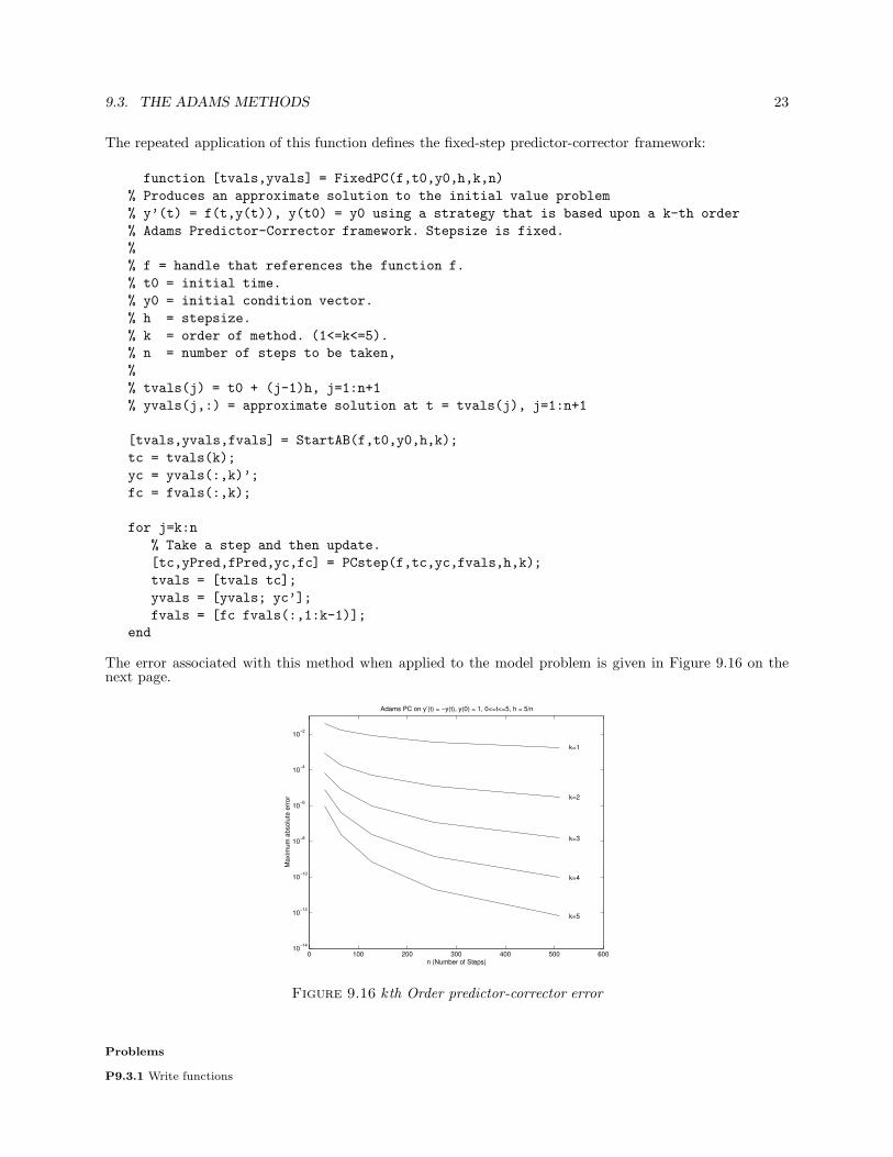
The error associated with this method when applied to the model problem is given in Figure 9.16 on thenext page.

0 100 200 300 400 500 60010

−14

10−12

10−10

10−8

10−6

10−4

10−2

Adams PC on y’(t) = −y(t), y(0) = 1, 0<=t<=5, h = 5/n

n (Number of Steps)

Ma

xim

um

ab

so

lute

err

or

k=1

k=2

k=3

k=4

k=5

Figure 9.16 kth Order predictor-corrector error

Problems

P9.3.1 Write functions


[tvals,yvals] = AFixedAB(A,t0,y0,h,k,n)

[tvals,yvals] = AFixedAM(A,t0,y0,h,k,n)

that can be used to solve the IVP y′(t) = Ay(t), y(t0) = y0, where A is a d-by-d matrix. In AFixedAM a linear system will haveto be solved at each step. Get the factorization “out of the loop.”

P9.3.2 Use FixedAB and FixedPC to solve the IVP described in problem P9.2.3. Explore the connections between step size,

order, and the number of required function evaluations.

9.3.5 Stepsize Control

The idea behind error estimation in adaptive quadrature is to compute the integral in question in two ways,and then accept or reject the better estimate based on the observed discrepancies. The predictor-corrector

framework presents us with a similar opportunity. The quality of y(C)n+1 can be estimated from |y

(C)n+1 − y

(P)n+1|.

If the error is too large, we can reduce the step. If the error is too small, then we can lengthen the step.Properly handled, we can use this mechanism to integrate the IVP across the interval of interest with stepsthat are as long as possible given a prescribed error tolerance. In this way we can compute the requiredsolution, more or less minimizing the number of f evaluations. The Matlab IVP solvers ode23 and ode45

are Runge-Kutta based and do just that. We develop a second-order adaptive step solver based on thesecond-order AB and AM methods.

Do we accept y(C) as our chosen yn+1? If ∆ = |y(P)n+1 − y

(C)n+1| is small, then our intuition tells us that

y(C)n+1 is probably fairly good and worth accepting as our approximation to y(tn+1). If not, there are two

possibilities. We could refine y(C)n+1 through repeated application of the AM2 formula:

yn+1 = y(C)n+1

Repeat:

yn+1 = yn + h2 (f(tn+1, yn+1) + fn)

A reasonable termination criterion might be to quit as soon as two successive iterates differ by a small amount.The goal of the iteration is to produce a solution to the AM2 equation. Alternatively, we could halve h andtry another predict/correct step [i.e., produce an estimate yn+1 of y(tn +h/2)]. The latter approach is moreconstructive because it addresses the primary reason for discrepancy between the predicted and correctedvalue: an overly long step h.

To implement a practical step size control process, we need to develop a heuristic for estimating the error

in y(c)n+1 based on the discrepancy between it and y

(P)n+1. The idea is to manipulate the LTE expressions

y(tn+1) = y(P)n+1 +

5

12h3y(3)(η1), η1 ∈ [tn, tn + h]

y(tn+1) = y(C)n+1 −

1

12h3y(3)(η2), η2 ∈ [tn, tn + h]

We make the assumption that y(3) does not vary much across [tn, tn + h]. Subtracting the first equationfrom the second leads to approximation

|y(C)n+1 − y

(P)n+1| ≈

1

2h3|y(3)(η)|, η ∈ [tn, tn + h]

and so

|y(C)n+1 − y(tn+1)| ≈

1

6|y

(C)n+1 − y

(P)n+1|.

This leads to the following framework for a second-order predictor-corrector scheme:

y(P)n+1 = yn + h

2 (3fn − fn−1)

y(C)n+1 = yn + h

2

(

f(tn+1 , y(P)n+1 + fn

)

ε = 16 |y

(C)n+1 − y

(P)n+1|


If ε is too big, then

reduce h and try again.

Else if ε is about right, then

set yn+1 = y(C)n+1 and keep h.

Else if ε is too small, then

set yn+1 = y(C)n+1 and increase h.

The definitions of “too big,” “about right,” and “too small” are central. Here is one approach. Suppose wewant the global error in the solution snapshots across [t0, tmax] to be less than δ. If it takes nmax steps tointegrate across [t0, tmax], then we can heuristically guarantee this if

nmax∑

n=1

LTEn ≤ δ.

Thus if hn is the length of the nth step, and

|LTEn| ≤hnδ

tmax − t0,

thennmax∑

n=1

LTEn ≤

nmax∑

n=1

hnδ

tmax − t0≤ δ.

This tells us when to accept a step. But if the estimated LTE is considerably smaller than the threshold,say

ε ≤1

10

δh

tmax − t0,

then it might be worth doubling h.If the ε is too big, then our strategy is to halve h. But to carry out the predictor step with this step size,

we need f(tn − h/2, yn−1/2) where yn−1/2 is an estimate of y(tn − h/2). “Missing” values in in this settingcan be generated by interpolation or by using (for example) an appropriate Runge-Kutta estimate.

We mention that the Matlab IVP solver ode113 implements an Adams-Bashforth-Moulton predictor-corrector framework.

Problems

P9.3.3 Derive an estimate for |y(C)n+1 − y(tn+1)| for the third-, fourth- and fifth-order predictor-corrector pairs.

M-Files and References

Script Files

ShowTraj Shows family of solutions.ShowEuler Illustrates Euler method.ShowFixedEuler Plots error in fixed step Euler for y’=y, y(0)=1.ShowTrunc Shows effect of truncation error.EulerRoundoff Illustrates Euler in three-digit floating point.ShowAB Illustrates FixedAB.ShowPC Illustrates FixedPC.ShowRK Illustrates FixedRK.ShowMatIVPTools Illustrates ode23 and ode45 on a system.


Function Files

FixedEuler Fixed step Euler method.ABStart Gets starting values for Adams methods.ABStep Adams-Bashforth step (order <= 5).FixedAB Fixed step size Adams-Bashforth.AMStep Adams-Moulton step (order <= 5).PCStep AB-AM predictor-corrector Step (order <= 5).FixedPC Fixed stepsize AB-AM predictor-corrector.RKStep Runge-Kutta step (order <= 5).FixedRK Fixed step size Runge-Kutta.Kepler For solving two-body IVP.f1 The f function for the model problem y’=y.

References

C.W. Gear (1971). Numerical Initial Value Problems in Ordinary Differential Equations, Prentice Hall,Englewood Cliffs, NJ.

J. Lambert (1973). Computational Methods in Ordinary Differential Equations, John Wiley, New York.

J. Ortega and W. Poole (1981). An Introduction to Numerical Methods for Differential Equations, Pitman,Marshfield, MA.

L. Shampine and M. Gordon (1975). Computer Solution of Ordinary Differential Equations: The Initial

Value Problem, Freeman, San Francisco.

Documents

The Initial Value Problem - Cornell University