Creating Initial Solutions for the TailAssignment ProblemMaster’s thesis in Computer Science — Algorithms, Languages and Logic

ELIN BLOMGREN

Department of Computer Science and EngineeringCHALMERS UNIVERSITY OF TECHNOLOGYUNIVERSITY OF GOTHENBURGGothenburg, Sweden 2018

Master’s thesis 2018

Creating Initial Solutions for theTail Assignment Problem

ELIN BLOMGREN

Department of Computer Science and EngineeringChalmers University of Technology

University of GothenburgGothenburg, Sweden 2018

Creating Initial Solutions for the Tail Assignment ProblemELIN BLOMGREN

© ELIN BLOMGREN, 2018.

Supervisor: Birgit Grohe, Department of Computer Science and EngineeringSupervisor: Ann-Brith Strömberg, Department of Mathematical SciencesAdvisor: Viktor Almqvist, JeppesenExaminer: Devdatt Dubhashi, Department of Computer Science and Engineering

Master’s Thesis 2018Department of Computer Science and EngineeringChalmers University of Technology and University of GothenburgSE-412 96 GothenburgTelephone +46 31 772 1000

Typeset in LATEXGothenburg, Sweden 2018

iv

Creating Initial Solutions for the Tail Assignment ProblemELIN BLOMGRENDepartment of Computer Science and EngineeringChalmers University of Technology and University of Gothenburg

AbstractOne of many optimization problems in the airline industry is the tail assignmentproblem, i.e. to decide which aircraft operate which flight. Initial solutions can beused to warm-start optimization algorithms. In this thesis, the optimization algo-rithm uses a time window heuristic together with column generation. This thesisinvestigates different methods to create initial solutions for the tail assignment prob-lem. The chosen methods consist of greedy algorithms and other simple heuristics.The goal was that the methods should assign at least 95% of the flights and thisis achieved by most methods and test cases. Also, when using the produced initialsolutions as input to the optimization algorithm, the value of the objective functionis improved for some of the test cases.

Keywords: airline optimization, heuristics, greedy, initial solution, tail assignment,aircraft routing, column generation, warm-start of algorithms.

v

AcknowledgementsFirstly, I want to thank Jeppesen for letting me do my thesis at their office and forproviding me with the necessary resources. I especially want to thank my supervisorViktor Almqvist for the meaningful discussions about my work and for always tak-ing the time to help me. I also want to thank Mattias Grönkvist who has supportedme during the thesis.

I want to thank the optimization teams as well as everyone else at the Jeppesenoffice who have shown interest in the project and to my roommate at Jeppesen,Emily Curry, for keeping me company and cheering me up when the thesis work washard.

At Chalmers, I want to thank my examiner Devdatt Dubhashi and my two super-visors Birgit Grohe and Ann-Brith Strömberg for their feedback on my thesis workand especially on the writing of the report.

Elin Blomgren, Gothenburg, June 2018

vii

Glossary

Task A flight, a maintenance, a sequence of tasks or some otheractivity that should be assigned to an aircraft

Roster A sequence of tasks that is assigned to an aircraft

Pre-assigned task A task that is locked to a specific aircraft

Free task A task that is not pre-assigned to any aircraft

Acronyms

AFR Aircraft First Random method

AFS Aircraft First Sort method

AFM Aircraft First Maintenance method

TFR Task First Random method

TFS Task First Sort method

TFM Task First Maintenance method

IMP IMProvement method

DFS Depth First Search

LP Linear Program

ILP Integer Linear Program

MP Master Problem

RMP Restricted Master Problem

ix

Notation

A The set of all aircraft

C The set of all cumulative rules

f ∈ F A task in the set of all tasks

r ∈ R The roster in the set of all rosters

Fr ⊆ F The set of tasks in roster r

ar ∈ A The aircraft assigned to roster r

tstartf The starting time of task f

tendf The ending time of task f

pstartf The starting position of task f

pendf The ending position of task f

x

Contents

1 Introduction 11.1 Aim and Limitations . . . . . . . . . . . . . . . . . . . . . . . . . . . 21.2 Literature Review . . . . . . . . . . . . . . . . . . . . . . . . . . . . . 21.3 Thesis Outline . . . . . . . . . . . . . . . . . . . . . . . . . . . . . . . 3

2 Theory 52.1 Integer Linear Programs . . . . . . . . . . . . . . . . . . . . . . . . . 52.2 Column Generation . . . . . . . . . . . . . . . . . . . . . . . . . . . . 62.3 Greedy Algorithms . . . . . . . . . . . . . . . . . . . . . . . . . . . . 7

3 Tail Assignment 93.1 Problem Description . . . . . . . . . . . . . . . . . . . . . . . . . . . 9

3.1.1 Tasks and Notation . . . . . . . . . . . . . . . . . . . . . . . . 93.1.2 Constraints and Maintenance . . . . . . . . . . . . . . . . . . 103.1.3 Objective . . . . . . . . . . . . . . . . . . . . . . . . . . . . . 11

3.2 Optimization Models . . . . . . . . . . . . . . . . . . . . . . . . . . . 123.3 Solving Tail Assignment Using Time Windows . . . . . . . . . . . . . 13

4 Heuristics to Create Initial Solutions 154.1 Legal Connections . . . . . . . . . . . . . . . . . . . . . . . . . . . . . 164.2 Fill Gaps Between Pre-assigned Tasks . . . . . . . . . . . . . . . . . . 174.3 Greedy methods . . . . . . . . . . . . . . . . . . . . . . . . . . . . . . 18

4.3.1 Aircraft First . . . . . . . . . . . . . . . . . . . . . . . . . . . 194.3.2 Tasks First . . . . . . . . . . . . . . . . . . . . . . . . . . . . 20

4.4 Methods for Hard Cumulative Constraints . . . . . . . . . . . . . . . 214.4.1 Aircraft First with Hard Cumulative Constraints . . . . . . . 214.4.2 Task First with Hard Cumulative Constraints . . . . . . . . . 22

5 Tests and Results 255.1 Results for Test Cases Without Hard Cumulative Constraints . . . . 265.2 Results for Cases With Hard Cumulative Constraints . . . . . . . . . 28

6 Discussion and Conclusion 33

Bibliography 37

xi

Contents

xii

1Introduction

There are many decisions to be made at an airline. One important problem is todecide which aircraft should operate which flight. To do this, one has to consider op-erational constraints such as maintenance, airport curfews, and aircraft restrictions.This problem is called tail assignment [1]. In addition to satisfying all rules andconstraints, the problem can be modeled to minimize fuel consumption, maximizeaircraft utilization, increase robustness, etc., in order to find savings and increasethe reliability of the airline’s operation.

This thesis is done in collaboration with Jeppesen in Gothenburg. Jeppesen is asubsidiary of The Boeing Company and provides planning and optimization toolsfor airlines. One of their products is a tail assignment optimizer which is the startingpoint for this thesis.

Aircraft operating costs are the by far biggest operating cost for airlines [2, Chapter6]. The single largest cost in this category is fuel. Further, the total cost of delayedflights in US in 2007 was estimated to be $31.2 billion [2, Chapter 10]. Makingrobust schedules that minimize the delays and their consequences is therefore animportant way to find savings for airlines. Different airlines prioritize costs and ro-bustness differently. By modeling robustness and other qualities as costs, Jeppesen’sproducts allow the airlines to choose which qualities that are most important andthe optimizer finds a solution targeted to minimize the cost.

The tail assignment problem is an NP-hard optimization problem [1, Section 4.2],which means that it can sometimes be very computationally demanding to find goodsolutions. To find good enough solutions as quickly as possible, Jeppesen’s optimizeruses a hybrid column generation and local search solution approach. The problem’splanning period is divided into time windows, and the problem is solved using columngeneration in a sequence of time windows which ’slide’ over the planning period togradually cover the full period.

To improve the performance of the currently in use optimizer at Jeppesen, an initialsolution that covers the entire planning period can be used as input to the optimizer.Producing solutions fast is also good because the user of the system gets feedbackalmost immediately and the user can also see if the problem data and rules workcorrectly. This thesis will investigate methods to create initial solutions and evaluatethem on real problems from different airlines.

1

1. Introduction

1.1 Aim and Limitations

The goal of this thesis is to find and implement a method that can be used tocreate initial solutions to warm start an improvement method. Since it can behard to assign all flights for complex problem instances, the goal is that the initialsolutions should have at least 95% of the flights assigned. All other hard constraints(explained in Section 3.1.2) must be satisfied. The aim is that the current optimizerat Jeppesen can produce better solutions if given an initial solution produced withthe developed method, than without an initial solution. The method also needs tobe fast and scalable to be able to support large airlines.

The main limitation of this thesis is that the methods developed in this thesis donot aim at finding the optimal solution. Since the produced solutions will be usedas initial solutions to an improvement method, it is enough that it is a legal solutioncovering the whole planning period (but with some flights unassigned).

The testing will be limited to a few problem instances from Jeppesen’s test suite.The final aim is that the method should work for all possible instances, but for thescope of this thesis there will be a smaller selection of problem instances for theevaluation.

1.2 Literature Review

Grönkvist [1] presented a constraint programming approach as well as a columngeneration approach to solve the tail assignment problem. Later, Gabteni andGrönkvist [3] combined these approaches to quickly find initial solutions as well asto improve the solution quality. Two difficulties with their approach are that it doesnot work if there is no feasible solution and that it does not consider maintenanceor other cumulative constraints.

One of the most recent publications on tail assignment is Khaled et al. [4]; it presentsa compact model of tail assignment which is solved to optimality. The bigger in-stances are, however, not solved to optimality when the maintenance constraints areadded. There is only one type of maintenance considered in [4]. and their biggestinstance only has 40 aircraft and 1494 flights.

Sarac et al. [5] present a branch-and-price method to the operational aircraft main-tenance routing problem. A problem that is similar to tail assignment, but withthe main difference that the planning horizon is shorter. In [5] only one day wasused and their objective was to minimize the number of unused legal flying hours.However, the first steps in their method for creating initial solutions are similar tothe ones presented in this thesis in the way that the aircraft are sorted and that thefirst possible connection is chosen iteratively.

Another solution method for aircraft maintenance routing proposed by Safaei and

2

1. Introduction

Jardine [6] includes a connection network Integer Linear Program (ILP) that handlesvarious maintenance tasks. They only solve the problem for one week at a time for afleet with up to 18 aircraft. Another difference is that they allow non-revenue flightsto transport aircraft to maintenance locations.

Column generation is a frequently used approach for many airline problems [1], [5],[7], [8]. However, Amin Jamili [9] and Deng and Lin [10] are two examples of theuse of stochastic optimization algorithms [11].

A similar problem to tail assignment is railway rolling stock assignment, the problemof assigning train-sets to utilization paths. Lai et al. [12] focused on the maintenancefor rolling stock and showed good results with a heuristic approach. Among othertechniques, their algorithm start with the trains that need maintenance the soonest.However, their routes are already aggregated into trips that all begin and end at thesame location which makes the problem easier to solve.

Creating initial feasible solutions for different operations research problems is oftena domain specific task. Several articles on initial solutions are published in differentdomains. For example, Juman and Hoque [13] for the transportation problem andJoubert and Claasen [14] for the constrained vehicle routing problem. Also, Guedesand Borenstein [15] show that a good initial solution improved the running timessignificantly for the multiple-depot vehicle type scheduling problem.

Tail assignment can be modeled as an integer multi-commodity network flow prob-lem with resource constraints [1, Model 4.1]. Dai et al. [16] proposed several ap-proaches to initial solutions for the multi commodity network flow problem. Thesewill, however, not work very well in the tail assignment setting since the authorsin [16] focus on problem instances with more commodities than nodes, which wouldcorrespond to more aircraft than flights. Also, the resource constraints and theintegrality constraints would have to be relaxed.

1.3 Thesis Outline

In Chapter 2 the theory used for both Jeppesen’s current solver as well as for themethods proposed in this thesis is explained. After that follows a more in-depthproblem definition in Chapter 3. In Chapter 4, the methods developed in this thesisare presented, followed by the tests and results in Chapter 5. Finally, the thesis isconcluded in Chapter 6.

3

1. Introduction

4

2Theory

This chapter describes the theory used for different solution methods for the tailassignment problem. Section 2.1 describes a common way to model integer linearoptimization problems and Section 2.2 describes one way to solve these optimizationproblems. These techniques are currently in use at Jeppesen. Section 2.3 describesthe theory behind the main algorithm proposed in this thesis.

2.1 Integer Linear Programs

Linear Programs (LP) are a way to model optimization problems with continuousvariables, linear constraints and linear objective function [17, Chapter 4.3]. Letx be a vector of n variables and c be a vector with corresponding costs for eachvariable. The m number of linear constraints for the variables x are expressed inthe constraint matrix A ∈ Rm×n together with the vector b ∈ Rm with the boundfor each constraint. Then a standard LP is of the form

min cᵀx, (2.1a)s.t. Ax = b, (2.1b)

x ≥ 0. (2.1c)

The goal is to minimize the cost (2.1a) subject to a set of linear equality (or inequal-ity) constraints (2.1b), where constraint i is defined as Aix = bi.

One of the most widely used methods to solve LPs is the Simplex method [18]. Eventhough the worst case complexity of the Simplex method is exponential in theory,it has been proved that the so called smoothed complexity is polynomial [19], [20].Examples of other solution methods are the ellipsoid method and interior pointmethods [21].

Integer Linear Programs (ILP) are special kinds of LPs where the variables musthave integer values. Therefore, there is also a constraint on the form x ∈ X, where

5

2. Theory

X ⊆ Zn. For a binary ILP, X = {0, 1}n and a standard binary ILP is of the form

min cᵀx, (2.2a)s.t. Ax = b, (2.2b)

x ∈ {0, 1}n. (2.2c)

In contrast to LP, which can be solved efficiently, ILPs are generally NP-hard andno efficient algorithm is known [22]. An ILP can be relaxed to allow continuousvalues of the variables. Such a re-formulated problem is called an LP-relaxation ofthe ILP. The LP-relaxation can be solved efficiently (e.g. by the Simplex method)but this will of course in general produce continuous solutions that is not feasiblefor the ILP.

One common exact method to solve ILP is Branch-and-bound [23, Section 8] whererelaxed problems are solved repeatedly in a tree-structure. In each node, the feasibleregion is divided into two parts, which becomes two branches. Both the lower andupper bound are stored in each node and a branch is pruned if it is not possible(calculated by the bounds) that the optimal solution can be found in a sub-branchof the node.

2.2 Column Generation

Column generation is a method that can be used to solve large scale LPs andILPs [24]. To apply column generation, it is necessary to first reformulate theproblem into two problems. These are a master problem (MP) and one or moresub problems (also called pricing problems). For example, the resource constrainedshortest path problem [25] can be modeled with a decision variable for each edge.When reformulated, a decision variable in the MP will instead represent a possiblepath through the network. Each decision variable in the MP is associated with apath through the network and is represented by a cost coefficient in the objective anda column in the constraint matrix. The number of paths is typically very large andtherefore only a subset of the paths are generated. The sub-problems are then usedto generate new possible paths (columns) with negative reduced cost (i.e. columnsthat can improve the objective) to the restricted master problem (RMP). This isrepeated for a predefined number of iterations or until the sub-problems do not findany improving columns.

During the iterations, the RMP passes new (dual) information to the sub-problemsand the sub-problems passes new improving columns to the RMP. But to initializethe iterations, a set of initial feasible columns is needed [26]. These can be definedusing so-called artificial variables [27], one for each constraint, each with a high cost,or, one can find initial solutions in other ways.

The RMP is solved as an LP. If the actual problem is an ILP one has to use somefixing heuristic to find an integer solution. Barnhart et al. [28] combine column

6

2. Theory

generation with branch-and-bound to solve large-scale ILP and the resulting methodis called branch-and-price.

2.3 Greedy Algorithms

Greedy algorithms always make the choice that is best (according to some criteria)at the moment [29]. In general, greedy algorithms are not guaranteed to find anoptimal solution, but for some problems there exists greedy algorithms that alwaysfind optimal solutions. For other problems, greedy algorithms can be used to findgood feasible solutions.

Generally, one can define a greedy algorithm with three sets and four functions [30].The starting point is a set C of all possible candidates and two empty sets, one forthe solution S and one with discarded candidates D. As the algorithm proceeds,candidates from the set C will be moved to S or D. A selection function decideswhich candidate c ∈ C is most promising and a feasibility function checks if a set ofcandidates can form a solution by adding more candidates. There is also a functionthat checks if a set of candidates form a complete solution and finally an objectivefunction that gives a solution an objective value. A scheme of a general greedyalgorithm is shown in Algorithm 1.

Algorithm 1: Greedy scheme1 S ← ∅2 D ← ∅3 while C 6= ∅ and not isSolution(S) do4 x← select(C)5 C ← C \ {x}6 if isFeasible(S ∪ {x}) then7 S ← S ∪ {x}8 else9 D ← D ∪ {x}

10 end11 end12 if isSolution(S) then13 return (S, objective(S))14 end

The algorithm selects in each iteration the best candidate c ∈ C according to theselection function. This candidate is removed from C and if it is feasible to add tothe solution S, it is added. Otherwise it is discarded and placed in D. After eachiteration, the algorithm checks whether or not the set S forms a complete solution.When either the set of candidates is empty or the set S forms a complete solution,the algorithm terminates and returns S as the solution, optionally together with theobjective value of the solution.

7

2. Theory

8

3Tail Assignment

Aircraft are identified by their tail-number, which is why the problem studied in thisthesis is called tail assignment. Tail assignment is an optimization problem and thegoal is to assign aircraft to all flights while optimizing some objective. Section 3.1describes the tail assignment problem and Section 3.2 describes different modelsused when solving tail assignment.

One of the main differences between Jeppesen’s optimizer and others seen in liter-ature is that Jeppesen’s optimizer has a very flexible way to model the constraintsand the objective function. Therefore, it is hard to make a specific definition of thecomponents of the problem since these tend to vary between airlines. This chapteraims at describing the components in general.

3.1 Problem Description

Tail assignment is solved for a specific planning period, which means that there is astart and end date. Typically this is about a month but it can be both shorter andlonger.

3.1.1 Tasks and Notation

Flights and maintenance checks are modeled as tasks, denoted by f . A task can alsobe a composite of other tasks. The set F consists of all tasks f that are scheduledin the planning period. Each task f ∈ F has a start time tstart

f and an end time tendf .

Each task f also has a starting position pstartf and an end position pend

f . In principle,a task can be anything possessing these attributes.

A roster is a sequence of tasks that belong to a specific aircraft. Let A be the setof all aircraft and R the set of all rosters. Then, the aircraft assigned to the rosterr ∈ R is denoted by ar ∈ A. The sequence of tasks belonging to roster r is Fr ⊆ F .Since a roster is simply a sequence of tasks and a task can be a composite of tasks,the same notation as for tasks is used for the roster attributes, i.e. tstart

r etc.

9

3. Tail Assignment

Some tasks are pre-assigned, which means that they are locked to a specific aircraft.There are two types of pre-assigned tasks. The first type is carry-ins, which arethe tasks that are scheduled before the planning period begins and states where theaircraft is in the beginning of the planning period. The second type is pre-scheduledmaintenance, typically the bigger ones that lasts for at least one week. Differentmaintenance types are explained in the next section.

An example solution to tail assignment is illustrated in Figure 3.1. The exampleconsists of four aircraft and a planning horizon of four days. The gray tasks arepre-assigned and locked to the aircraft. The blue tasks are so-called free tasks, forwhich it is up to the optimizer to decide which aircraft the task should be assignedto. The pre-assigned task at day 3 is an example of pre-assigned maintenance whichis described below.

X Y Pre-assigned task X Y Free task

Day 1 Day 2 Day 3 Day 4

Air

craf

t/R

ost

er

1

2

3

4

C A

C D

B B

D AA D

D C

D CA C C A

C AB C

A D

A C

A B

D A A D D A

B A

A BC B

A D D A

B A

C AB C

C DA C

Figure 3.1: An example of a solution to a tail assignment problem. The tasks areboxes with a starting position and an ending position.

Pre-assigned tasks may result in gaps in the roster between the pre-assigned tasks.For example, the roster for aircraft 3 in Figure 3.1 had a gap between the pre-assigned tasks at day 1 and 3, before the free tasks were assigned to the aircraft.

3.1.2 Constraints and Maintenance

At Jeppesen, all rules concerning flights, airports, tasks, aircraft, maintenance etc.are written in Rave [31]. Rave is a domain specific language developed at Jeppesen.The optimizer has access to a general interface to Rave where certain questions canbe asked. For example, if a task is legal for a specific aircraft or to get the connectioncost between two tasks.

There are different kinds of maintenance for aircraft. The most extensive kind ofmaintenance is done every one to three years and can take up to a month. Thesmallest maintenance might be performed every day (night) and may take aboutan hour. Between these extreme cases, there are a lot of intermediate maintenancelevels. The maintenance regulations vary between airlines and countries and multiplemaintenance levels can be used by the same airline.

10

3. Tail Assignment

When modeling tail assignment, there are two ways to model the maintenance rules.The first way is as pre-assigned tasks, which means that the maintenance’s time andplace are not decided by the optimization process but instead decided on before-hand. Usually, it is the bigger and less frequent maintenance that is modeled inthis way. The second way is with cumulative constraints, which are usually usedfor the more frequent maintenance types that are performed several times duringthe planning period. The same problem instance can have both kinds of rules fordifferent maintenance levels.

Cumulative constraints are the most complex rules since they depend on the historyof the aircraft (e.g. it is needed to keep track of when the aircraft last had mainte-nance of a certain type). Cumulative constraints are modeled as resource constraintswhere the resource for example can be time, flight hours, or number of landings. Ifthe consumption of the resource exceeds a defined limit, the constraint is violated.The most common way to reset the consumption of the resource is to make surethat the aircraft spends a number of hours on the ground at one in a subset of theairports (e.g. at which it is possible to perform maintenance). The set of cumulativeconstraints are denoted by C.

There are both soft and hard constraints. The hard constraints simply state thatsomething is impossible and that a solution that breaks any hard constraint is illegal.The soft constraints are modeled with a penalty cost (in the objective) for violatingthe constraint.

Since tail assignment can be solved simultaneously for multiple fleets, it can some-times be cost-worthy to re-fleet a flight. Re-fleeting means that a flight is assignedto an aircraft of a different type than it was originally planned for. Re-fleeting canbe modeled as a soft constraint where the penalty for violating the constraint is thecost of changing aircraft type.

Sometimes there are also global constraints, which apply when something is depen-dent on more than one aircraft. The most recurring global constraint is to havea limit on the number of aircraft that receive maintenance simultaneously at thesame airport. Another example is to require a minimum number of aircraft on theground, to use if disturbances occur.

3.1.3 Objective

Different objectives can be used when solving the tail assignment problem. Theobjective can be to minimize actual costs, such as fuel consumption, or fictive costs,which for example will favor robust solutions or other qualities that the airlinedesires. Often both actual and fictive costs are used in combination.

The objective function is also modeled in Rave and is to be defined by the user ofthe system. If the problem instance does not have a solution covering all flights, thecost of unassigned tasks is often the biggest part of the total cost. Another part

11

3. Tail Assignment

that often influences the cost is fuel consumption and the connection time betweenflights. An example of a connection cost function that can be used to reduce mediumlength connections is found in [1, Section 13.1]. When soft constraints are employed,the penalty for violating these are also part of the cost.

3.2 Optimization Models

There are multiple ways to model the tail assignment problem. Grönkvist [1]presents three main models. First, there is an integer multi-commodity networkflow problem formulation [1, Model 4.1]. This is perhaps the most intuitive formula-tion but it is not used very often when solving the tail assignment problem. Further,there is a set partitioning formulation [1, Model 4.2]. This is a very useful modelthat can be solved by column generation and is explained below. The last model isa constraint satisfaction problem model [1, Model 9.2] that Grönkvist later uses foraccelerating the column generation [32]. This can be done since all three of thesemodels express the same problem in different ways and a solution to one formulationcan always be transformed into a solution to the others.

Let R be the set of all legal aircraft rosters, xr be the decision variable of whetheror not roster r ∈ R is taken and cr be the cost of roster r. Further, the constantαfr is 1 if task f is covered by roster r and 0 otherwise. Then, tail assignment canbe modeled as a set partitioning problem [1, Model 4.2]

min∑r∈R

crxr, (3.1a)

s.t.∑r∈R

αfrxr = 1, ∀f ∈ F, (3.1b)

xr ∈ {0, 1}, ∀r ∈ R. (3.1c)

The goal as specified in (3.1a) is to choose xr, r ∈ R such that the total cost isminimized. In this problem formulation there are two sets of constraints. In (3.1b)we ensure that each task is covered by a an aircraft and the integrality constraintsin (3.1c) ensure that xr is binary.

The complicating property of this formulation is that the set R is very large (expo-nential in the number of tasks) and also hard to find [1, Section 4.4 and 5.2]. Thecurrent approach to solve this is to use column generation (see Section 2.2). TheRMP is the LP-relaxed (i.e. (3.1c) changed to xr ≥ 0) version of (3.1) but withthe subset R′ ⊆ R instead of R. The pricing problem is then used to generate newrosters to R′ (i.e., new columns, consisting of αfr, f ∈ F , and cr). This problem ismodeled in a graph as a resource constrained shortest path problem [1, Section 5.3]to ensure that the generated rosters satisfy all the constraints. Some constraints areenforced by the connections between nodes. The cumulative constraints (e.g. main-tenance) are modeled with the resources in the pricing problem. For more details,see [1, Section 5.3–5.4].

12

3. Tail Assignment

3.3 Solving Tail Assignment Using Time Windows

At Jeppesen, most problem instances are divided into multiple smaller so-calledtime windows for which column generation is performed individually [1, Section12.3]. Usually the size of the windows are between one and seven days. One sweepthrough the planning period goes through all time windows once in order. The timewindows have some overlap that is decided per customer. After one sweep, the timewindows can be altered so that the breakpoints occurs at different places in the nextsweep.

For each time window, there are some locked tasks in the beginning and in the end.The rosters generated in the column generation only cover this time window andconsists of a path between the start task and end task. If there is no initial solution,each time window only has one fixed task in the beginning, the end task is up tothe column generation to decide.

13

3. Tail Assignment

14

4Heuristics to Create Initial

Solutions

This chapter presents the developed methods to create initial solutions to the tail as-signment problem. The methods use heuristics to find solutions fast. The heuristicsused are greedy algorithms and depth first search (DFS) [33, Section 3.2].

The general method is divided into two stages. First, the gaps between pre-assignedtasks are handled using a method called FillGaps and then, in the second stage,the rosters are appended with more tasks using the method AppendRosters. Anexample that illustrates these stages are found in Figure 4.1. This means thatAppendRosters will assign tasks (if possible) after the last pre-assignment in eachroster. The general algorithm is presented in Algorithm 2.

Algorithm 2: General scheme1 Initialize A,F,R2 shuffle(R)3 FillGaps(R,F )4 AppendRosters(R,F )

The first row in Algorithm 2 is the initialization steps. First, the data (tasks F andaircraft A) is collected. Then, for each aircraft a ∈ A, a new roster r is createdwith only the pre-assigned tasks for ar. The rosters form the set R. The set F isordered by ascending start time. After that, the rosters are shuffled to avoid gettingthe same arbitrary order for each run of the algorithm. In this way, we can runthe algorithm multiple times and then choose the best solution. Row 3 handles thegaps between pre-assigned tasks and is explained in detail in Section 4.2. Finally,the method AppendRosters on row 4 is done in several different ways, which aredescribed in Sections 4.3 and 4.4. Section 4.1 describes how to determine whethera connection is legal, something that is used in many of the developed methods.

15

4. Heuristics to Create Initial Solutions

X Y Pre-assigned task X Y Free task

Day 1 Day 2 Day 3 Day 4

Air

craf

t/R

ost

er

1

2

3

4

B B

A D

D C

A C

B A

(a) The initial four rosters with only pre-assigned tasks.

Day 1 Day 2 Day 3 Day 4

Air

craf

t/R

ost

er

1

2

3

4

C A B B

A D

D C

A C

A B

B A

(b) The four rosters resulting from theapplication of the method FillGaps.

Day 1 Day 2 Day 3 Day 4

Air

craf

t/R

ost

er

1

2

3

4

C A

C D

B B

D AA D

D C

D CA C C A

C AB C

A D

A C

A B

D A A D D A

B A

A BC B

A D D A

B A

C AB C

C DA C

(c) The four rosters resulting fromthe application of the methodAppendRosters has been performed.

Figure 4.1: An example of how a solution is formed by the stages in the generalscheme.

4.1 Legal Connections

In many situations, there is a need to check if the connection between two tasks islegal. To see if the connection is legal, there are a number of conditions to check. Wedefine the function isLegal(f, g, a) to check the legality of the connection betweentasks f and g with respect to aircraft a. Note that the first task can be either aroster or a task. The following legality checks are performed:

1. Is the position pendf = pstart

g ?

2. Is the time tendf ≤ tstart

g ?

3. Does aircraft a has the necessary requirements needed for task g?

16

4. Heuristics to Create Initial Solutions

4. Is task g is allowed for aircraft a according to the Rave model?

5. Is the connection between task f and g legal for aircraft a according to theRave model?

For a connection to be legal, all these checks must be true. The checks are performedin increasing order, so that the more time-consuming checks (which depend on theRave model) are only done if the previous checks were legal.

For check number 2, we assume a connection time of 0. In practice, a longer connec-tion time is needed, but since this depends on the task, the airport, and the aircraft,this is handled in Rave (check 5).

4.2 Fill Gaps Between Pre-assigned Tasks

Pre-scheduled maintenance create gaps in the rosters between the pre-assigned tasksin the beginning of the planning period and the later maintenance. This is one ofthe more difficult parts for the current optimizer. Therefore, it is important to findan algorithm that can fill these gaps efficiently.

The method FillGaps is shown in Algorithm 3. The algorithm loops through thetasks in each roster. The next task after f is denoted f + 1. For each task f in theroster r, a DFS inspired algorithm is used to find a sequence of tasks that fill thegap between tasks f and f +1. The tasks represent the nodes in the graph searchedby the DFS. The only difference from an ordinary DFS is that it only checks if thegoal is reached if there are no more possible tasks to add. The set V of visited nodes(tasks) is used to avoid visiting the same node more than once.

For each gap in the roster at hand, the algorithm will check all tasks g ∈ F , forwhich tstart

g is between tendf and tstart

f+1 , whether it is legal to assign task g after taskf . The algorithm also check that the task is uncovered and whether the inequalitytendg ≤ tstart

f+1 holds. If legal, the task g is appended to the roster r. When there areno more tasks to consider, the algorithm checks if the new connection in the roster,i.e. between f and f + 1, is legal. If it is not, the task f is removed from the rosterand put in the set of visited nodes V ← V ∪ {f}. Let f be the previous task in theroster and go through the steps again.

If there are two pre-assigned tasks for each roster, one in the very beginning of theplanning period and one in the very end, there are |A| gaps to fill with |F | − |A|potential tasks. These are considered by DFS, for which the time complexity isO(|nodes|+ |edges|); the nodes correspond to the potential tasks |F |−|A|, and thereare at most (|F | − |A|)2 edges. The resulting complexity is O(|A|(|F | − |A|)2) =O(|A||F |2 − 2|F ||A|2 + |A|3). Since |A| � |F |, this means that |A|3 < |A||F |2 andthe complexity can be written as O(|A||F |2). Note that this is a worst case analysisand this will probably not be the case for real problems.

17

4. Heuristics to Create Initial Solutions

Algorithm 3: FillGaps1 foreach r ∈ R do2 f ←first(r)3 V ← ∅4 while f 6= null do5 foreach g ∈ {g : g ∈ F ∧ tend

f ≤ tstartg ≤ tstart

f+1 } do6 if isLegal(f, g, ar) ∧ g /∈ V ∧ tend

g ≤ tstartf+1∧ isUncovered(g) then

7 insert(r, g)8 f ← g

9 end10 end11 if isLegal(f, f + 1, ar) then12 f ← f + 113 else14 remove(r, f)15 V ← V ∪ {f}16 f ← f − 117 end18 end19 end

4.3 Greedy methods

The methods to be presented in this section do not consider hard cumulative con-straints but only the ones checked in the function isLegal. The reason for this isto be able to use a fast greedy approach for the problem instances that does nothave hard cumulative constraints (see Section 4.4 for the corresponding algorithmsfor those cases). The four methods are all quite similar. These are Aircraft FirstRandom (AFR), Aircraft First Sort (AFS), Task First Sort (TFS) and Task FirstRandom (TFR). For the complete run of Algorithm 2, one of these is chosen as themethod AppendRosters.

Recall the notation used for the general greedy algorithm in Section 2.3. The candi-date set C is here the set of pairs (a, f) ∈ A× F (the Cartesian product of aircraftand tasks), the solution set S corresponds to R, in which the rosters are accumu-lated, and the set D of discarded candidates is accumulated implicitly by the waynew candidates are selected.

The selection function is implicit by the looping through the set of candidates. Thelooping order differs between the methods. The feasibility function is the functionisLegal and there is no explicit function checking if the solution is complete, sinceall the candidates will be considered. Finally, the objective function is the onedefined in the Rave model (as explained in Section 3.1.3).

18

4. Heuristics to Create Initial Solutions

4.3.1 Aircraft First

Each of the two methods AFR and AFS consists of a nested loop where the outerloop iterates through the aircraft/rosters and the inner loop iterates through thetasks.

Before these loops are executed, the aircraft are ordered in some way. For AFR,the aircraft are listed in random order and is therefore called Aircraft First Random(AFR), see Algorithm 4.

Algorithm 4: Aircraft First Random (AFR)1 shuffle(R)2 foreach r ∈ R do3 foreach f ∈ F do4 if isLegal(r, f , ar) ∧ isUncovered(f) then5 append(r, f)6 end7 end8 end

The other method AFS sorts the aircraft based on the number of restrictions (de-creasing) which is called Aircraft First Sort (AFS). Note that the solution producedby the method can differ between runs if multiple aircraft have the same number ofrestrictions, since ties are broken randomly.

Algorithm 5: Aircraft First Sort (AFS)1 sort(R)2 foreach r ∈ R do3 foreach f ∈ F do4 if isLegal(r, f , ar) ∧ isUncovered(f) then5 append(r, f)6 end7 end8 end

The shuffle step in AFR takes linear time (O(|A|)) and is done only once in thebeginning. Since the outer loop goes through each roster once, and there is oneroster for each aircraft, this loop consists of |A| iterations. The inner loop consistsof |F | iterations, where each iteration takes constant time. Hence, the resulting timecomplexity is O(|A||F |).

For AFS, the algorithm starts by sorting the aircraft/rosters which is done inO(|A| log(|A|)). However, to obtain the number of restrictions used for the sorting,O(|A||F |) computations are required. The resulting complexity is thenO(|A| log(|A|)+|A||F |). For practical problems, there are a lot more tasks than aircraft (i.e.

19

4. Heuristics to Create Initial Solutions

|A| � |F |). Therefore, the first term can be ignored and the complexity is thesame as for AFR, i.e. O(|A||F |).

4.3.2 Tasks First

The Aircraft First methods typically assign a lot more tasks to the first rosterscompared to the later rosters. Therefore, we present two methods that aim todistribute the tasks more evenly.

The difference between the Tasks First and Aircraft First methods is that the innerand outer loop have been swapped. Instead of looping over the rosters and foreach roster loop over all tasks, the algorithms loop over all tasks once and for eachtask over all the rosters. In this way, the inner loop may be exited when a legalassignment is found since only one aircraft should cover each task. To distribute thetasks evenly, the order of the rosters are shuffled for each task; see Algorithm 6.

Algorithm 6: Tasks First Random (TFR)1 foreach f ∈ F do2 shuffle(R)3 foreach r ∈ R do4 if isLegal(r, f , ar) ∧ isUncovered(f) then5 append(r, f)6 break7 end8 end9 end

An alternative is to re-sort the aircraft for each task. In this case, the sorting isbased on the number of tasks (ascending) in each roster to even better balance theload on each aircraft. This is shown in Algorithm 7; note that the only differencefrom Algorithm 6 is on row 2.

Algorithm 7: Tasks First Sort (TFS)1 foreach f ∈ F do2 sort(R)3 foreach r ∈ R do4 if isLegal(r, f , ar) ∧ isUncovered(f) then5 append(r, f)6 break7 end8 end9 end

20

4. Heuristics to Create Initial Solutions

For TFR, the outer loop consists of |F | iterations and in each iteration, the shufflestep takes O(|A|) time and the inner loop contains at most |A| iterations. Hence,the time complexity is O(|A||F |), the same as for AFR and AFS. For TFS, onthe other hand, the sorting is done in O(|A| log(|A|)) and the total complexity isO(|A||F | log(|A|)). As mentioned in the previous section, |A| � |F | and this extralog(|A|) factor should not influence the practical running time much.

4.4 Methods for Hard Cumulative Constraints

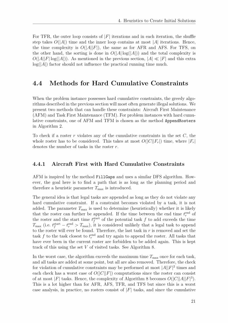
When the problem instance possesses hard cumulative constraints, the greedy algo-rithms described in the previous section will most often generate illegal solutions. Wepresent two methods that can handle these constraints: Aircraft First Maintenance(AFM) and Task First Maintenance (TFM). For problem instances with hard cumu-lative constraints, one of AFM and TFM is chosen as the method AppendRostersin Algorithm 2.

To check if a roster r violates any of the cumulative constraints in the set C, thewhole roster has to be considered. This takes at most O(|C||Fr|) time, where |Fr|denotes the number of tasks in the roster r.

4.4.1 Aircraft First with Hard Cumulative Constraints

AFM is inspired by the method FillGaps and uses a similar DFS algorithm. How-ever, the goal here is to find a path that is as long as the planning period andtherefore a heuristic parameter Tmax is introduced.

The general idea is that legal tasks are appended as long as they do not violate anyhard cumulative constraint. If a constraint becomes violated by a task, it is notadded. The parameter Tmax is used to determine (heuristically) whether it is likelythat the roster can further be appended. If the time between the end time tend

r ofthe roster and the start time tstart

f of the potential task f to add exceeds the timeTmax (i.e. tstart

f − tendr > Tmax), it is considered unlikely that a legal task to append

to the roster will ever be found. Therefore, the last task in r is removed and set thetask f to the task closest to tend

r and try again to append the roster. All tasks thathave ever been in the current roster are forbidden to be added again. This is kepttrack of this using the set V of visited tasks. See Algorithm 8.

In the worst case, the algorithm exceeds the maximum time Tmax once for each task,and all tasks are added at some point, but all are also removed. Therefore, the checkfor violation of cumulative constraints may be performed at most |A||F |2 times andeach check has a worst case of O(|C||F |) computations since the roster can consistof at most |F | tasks. Hence, the complexity of Algorithm 8 becomes O(|C||A||F |3).This is a lot higher than for AFR, AFS, TFR, and TFS but since this is a worstcase analysis, in practice, no rosters consist of |F | tasks, and since the cumulative

21

4. Heuristics to Create Initial Solutions

Algorithm 8: Aircraft First Maintenance (AFM)1 foreach r ∈ R do2 V ← ∅3 f ← first(F )4 while f 6= null do5 if tstart

f − tendr > Tmax then

6 removeLast(r)7 f ← min f ∈ F : tstart

f ≤ tendr

8 if isLegal(r, f , ar) ∧f /∈ V ∧ isUncovered(f) then9 if isCumulativeLegal(r, f, ar) then

10 append(r, f)11 V ← V ∪ f12 end13 end14 f ←next(F, f)15 end16 end

constraints are only evaluated if the connection is legal in all other aspects, thealgorithm will be faster in most practical settings.

AFM provides a simple way to handle all kinds of possible cumulative constraints. Itdoes not matter what resources are consumed in which tasks and how the resource isreset for each constraint (see Section 3.1.2). The only assumption is the maximumtime Tmax, which is a heuristic parameter whose value must be higher than themaximum reset time of any hard cumulative constraint and lower than an acceptableconnection time between tasks. Because of the way tail assignment is modeled atJeppesen, such detailed information about rules is not available in the interface tothe rule model. Instead, Tmax is manually set to one day.

4.4.2 Task First with Hard Cumulative Constraints

The method TFM is a naive approach that uses the same algorithm as TFR butin addition to the isLegal check, it also checks the hard cumulative constraints;see Algorithm 9. This approach does not always create rosters that cover the wholemonth, since the aircraft might be stuck at an airport where maintenance is notpossible to perform.

For the complexity analysis, the worst case occurs when all tasks are possible toassign to the last roster that is tried. As previously stated, the worst case for thecheck for cumulative constraints violation has a complexity of O(|C||F |). This istried at most |F ||A| times and the resulting time complexity is O(|C||A||F |2).

22

4. Heuristics to Create Initial Solutions

Algorithm 9: Tasks First Maintenance (TFM)1 foreach f ∈ F do2 shuffle(R)3 foreach r ∈ R do4 if isLegal(r, f , ar) ∧ isUncovered(f) then5 if isCumulativeLegal(r, f, ar) then6 append(r, f)7 break8 end9 end

10 end11 end

23

4. Heuristics to Create Initial Solutions

24

5Tests and Results

The methods described in Chapter 4 have been implemented in C++ in Jeppesen’sdevelopment environment. The testing has been done on a machine with Intel(R)Xeon(R) CPU E5-2667 v2 @ 3.30GHz. It has two times eight cores but only 8 areused per optimization run.

The different methods in Chapter 4 are evaluated on the test cases presented inTable 5.1. These differ in size in several ways. Cases 3 and 4 have the shortestplanning period, of one week, while the others have a planning period of just over amonth. They also differ in number of aircraft. Case 8 includes seven aircraft whilecase 5 includes 112 aircraft. Case 5 is also the largest in terms of number of tasks.

The first six cases have none or only soft cumulative constraints while cases 7 and8 have hard cumulative constraints.

The test cases have other differing characteristics, not shown in the table. Forexample, they have different rules, pre-assignments, and airports. They also havedifferent objective functions. Case 2 possesses only the unassigned task cost whilecases 3, 4, and 8 also have connection costs. The cases 1, 5, 6, and 7 have thesecosts as well as penalties for violating soft cumulative constraints.

#aircraft #tasks #days UB LBCase 1 15 2231 37 424 904 205Case 2 46 7730 36 740 775 0Case 3 71 3096 7 30 254 1 344Case 4 17 727 7 70 822 1 656Case 5 112 23825 32 2 372 428 64Case 6 65 6191 36 121 636 51Case 7 27 4388 34 16 407 766Case 8 7 1151 39 138 885 4 801

Table 5.1: Test cases with some basic characteristics. The columns represent thenumber of aircraft, the number of tasks, the length of the planning period, the upperbound (UB) (the cost of the initial solution with only pre-assigned tasks) and a lowerbound (LB) (see description in the text).

The lower bounds (LB) presented in Table 5.1 are calculated using a network flow

25

5. Tests and Results

model according to [1, Section 4.6]. This lower bound considers neither aircraftspecific connection rules nor aircraft specific costs. If everything can be assignedwithout these aircraft specific rules, the only cost in the lower bound will be theconnection cost since penalties for soft constraints (cumulative or global) cannot behandled efficiently in the network flow model. For all the test cases in Table 5.1except case 7, the lower bound solutions have all tasks assigned. Therefore, thelower bound consists of the connection cost only. The quality of the lower bounddiffers a lot between the test cases. For example, the lower bound for case 5 is muchlower than the optimal solution since the costs differ between aircraft and since nopenalties are included.

Our main focus has been on comparing the methods with each other but also withthe improvement method (IMP) developed by Jeppesen. IMP goes through theplanning period once, divided in time windows (as explained in Section 3.3). Thesize of the time windows varies between test cases but is the same for a single casewhen run with and without an initial solution.

Since all the methods described in Chapter 4 have some random components, eachmethod has been run 49 times each per test case in the evaluation. The greedymethods Aircraft First Random (AFR), Aircraft First Sort (AFS), Task First Sort(TFS), and Task First Random (TFR) are evaluated in Section 5.1 on test cases1–6. The methods Task First Maintenance (TFM) and Aircraft First Maintenance(AFM) are evaluated in Section 5.2 on test cases 7 and 8.

5.1 Results for Test Cases Without Hard Cumu-lative Constraints

The percentages of assigned tasks resulting from the test runs are shown in table 5.2for the different algorithms and test cases. Generally, the methods perform well,as compared to the goal of generating solutions having at least 95% of the tasksassigned. All the methods achieve this for all test cases except for case 3.

AFR AFS TFS TFRmed max med max med max med max

Case 1 99.5 99.7 99.7 99.7 99.5 99.7 99.5 99.7Case 2 99.5 99.6 99.2 99.2 99.4 99.5 99.2 99.5Case 3 89.5 93.2 90.0 93.4 89.3 92.7 89.5 92.6Case 4 97.7 97.9 97.7 97.7 97.7 97.7 97.7 97.9Case 5 99.4 99.4 99.4 99.4 99.1 99.1 99.4 99.7Case 6 98.9 99.5 99.0 99.0 98.9 99.6 98.8 99.5

Table 5.2: The percentage of assigned tasks for different test cases and methods.The best and median are presented. Underlined values are best in their category(med/max) per case.

26

5. Tests and Results

The costs for the initial solutions generated by the different methods are presentedin Table 5.3. For different test cases, different methods are best. If we look at thebest found solutions (with minimum cost), the results show that TFR and AFR arebest on two cases each while TFS and AFS are best on one each. On the otherhand, AFS is best on four cases if we look at the median cost.

AFR AFS TFS TFRmed min med min med min med min

Case 1 3 418 2 339 2 349 2 300 2 668 2 064 2 626 1 998Case 2 3 800 2 850 5 500 5 500 4 350 3 200 5 775 3 750Case 3 4 825 3 716 4 619 3 666 4 837 3 813 4 755 3 806Case 4 3 375 3 160 3 364 3 357 3 407 3 394 3 412 3 215Case 5 3 061 3 046 3 060 3 046 3 132 2 939 2 943 2 269Case 6 2 338 1 438 2 275 2 182 2 345 1 189 2 401 1 374

Table 5.3: The median and minimum costs of the solutions received for the differenttest cases and algorithms

The average computation times are presented in Table 5.4. The time is separatedbetween the appending methods (AFR, AFS, TFR, and TFS) and FillGaps. Toform a complete solution both FillGaps and one of the appending methods haveto be run and the total running time is the sum of the corresponding computationtimes. As can be seen, TFR is the fastest for all the cases, and for some cases TFS isequally fast. The randomizing variants (AFR, TFR) are also generally faster sinceshuffling is faster than sorting.

AFR AFS TFS TFR FillGapsCase 1 0.50 0.64 0.30 0.30 0.22Case 2 2.98 4.70 1.14 0.54 2.34Case 3 0.82 1.36 0.16 0.10 0.64Case 4 0.04 0.04 0.02 0.02 0.02Case 5 14.36 20.18 16.28 2.68 10.22Case 6 5.70 7.30 2.78 2.44 3.18

Table 5.4: The average computation time in CPU seconds for the different algo-rithms and test cases.

To set the running times in perspective, test case 5 takes almost one hour for themethod IMP, while test case 4 only takes a few seconds. Over all the methods takeno more than 1–2% of the running time as compared to that of IMP.

The average running times increase with the number of tasks and aircraft. Asdescribed in Section 4.3, the time complexity for AFR, AFS and TFR is O(|A||F |)and for TFS it is O(|A||F | log |A|). Even though TFS has a slightly higher theoreticalcomplexity, in practice, it is still generally faster than AFR and AFS.

Since the running time increases with both number of aircraft and tasks, it is rea-sonable that test case 5 has a lot longer running times than the other test cases.

27

5. Tests and Results

However, it is remarkable that TFR succeeds with that instance a lot faster thanthe other methods do.

The running times should only give a hint of the performance of the methods sincethere have been just a minimal effort to improve the running time by implementationdetails. However, there are a couple of reasons why TFR and TFS are faster thanAFR and AFS. The main reason is that the loop over aircraft is exited whenever afeasible assignment is found. AFS also calculates the number of restrictions, whichrequires a call to the Rave model (explained in Section 3.1.2) for each task/aircraftpair.

In Figure 5.1, the cost results are presented as bar charts. The costs are dividedinto connection cost, cost of unassigned tasks and the penalty for violating cumu-lative constraints. The labels indicates the cost components of each test case. Theconnection cost varies very little between the methods but the cost of unassignedtasks varies more.

The quality of the lower bound is not very good for test cases 1, 5, and 6, since allother solutions have much higher connection cost than the lower bound.

For each case, the four first bars represent the cost components of the median so-lution, as well as the 10th and 90th percentile (the black interval). The percentilevalues show that there is sometimes a big variation of results even if the minimumand median cost are similar, particularly the AFR and AFS for case 4 have a muchhigher 90th percentile than both the median and 10th percentile.

In Figure 5.1, the results for the methods are compared with Jeppesen’s methodIMP, running IMP with initial solutions and the lower bound. The best foundinitial solution by each method is used as input to IMP. As can be seen, the resultswhen using an initial solution is about the same or better as without an initialsolution.

Recall, from Table 5.2, that test case 3 has a lower percentage of assigned flightsthan the other cases. Still, the method IMP is able to find a solution with about thesame cost as the LB when running IMP with the ’bad’ initial solutions (Figure 5.1,Case 3).

The aircraft in test case 3 and 4 have almost all the same number of restrictions.Therefore, the result is very similar for AFS and AFR for these cases.

5.2 Results for Cases With Hard Cumulative Con-straints

The methods AFM and TFM (see Section 4.4) are evaluated on test cases 7 and 8from Table 5.1.

28

5. Tests and Results

Co

st

0

1000

2000

3000

4000

5000

6000

AFR AFS TFS TFR AFR

&

IMP

AFS

&

IMP

TFS

&

IMP

TFR

&

IMP

IMP LB

Co

stCase 1

Penalty

Unassigned

Connection

0

1000

2000

3000

4000

5000

6000

7000

8000

9000

AFR AFS TFS TFR AFR

&

IMP

AFS

&

IMP

TFS

&

IMP

TFR

&

IMP

IMP LB

Co

st

Case 2

Unassigned

Unassigned

0

1000

2000

3000

4000

5000

6000

AFR AFS TFS TFR AFR

&

IMP

AFS

&

IMP

TFS

&

IMP

TFR

&

IMP

IMP LB

Co

st

Case 3

Unassigned

Connection

0

1000

2000

3000

4000

5000

6000

AFR AFS TFS TFR AFR

&

IMP

AFS

&

IMP

TFS

&

IMP

TFR

&

IMP

IMP LB

Co

st

Case 4

Unassigned

Connection

0

500

1000

1500

2000

2500

3000

3500

4000

AFR AFS TFS TFR AFR

&

IMP

AFS

&

IMP

TFS

&

IMP

TFR

&

IMP

IMP LB

Co

st

Case 5

Penalty

Unassigned

Connection

0

500

1000

1500

2000

2500

3000

3500

AFR AFS TFS TFR AFR

&

IMP

AFS

&

IMP

TFS

&

IMP

TFR

&

IMP

IMP LB

Co

st

Case 6

Penalty

Unassigned

Connection

Figure 5.1: Bar plots of the result from the different greedy methods for sixtest cases, the solution with the median total cost is shown with the different costcomponents. The black interval represents the 10th and 90th percentiles, respectivly,of the total cost. The cost is also compared with Jeppesen’s method IMP; seedescription in the text.

The naive method TFM shows a huge variation in solution quality. This is shownboth in the percentages of assigned flights (Table 5.5) and the solution cost (Table5.6).

Both TFM and AFM achieve the goal of assigned tasks for both test cases withrespect to the best solution. For test case 8, AFM achieve the goal also with themedian solution.

The running times are presented in Table 5.7. The results from the two methods

29

5. Tests and Results

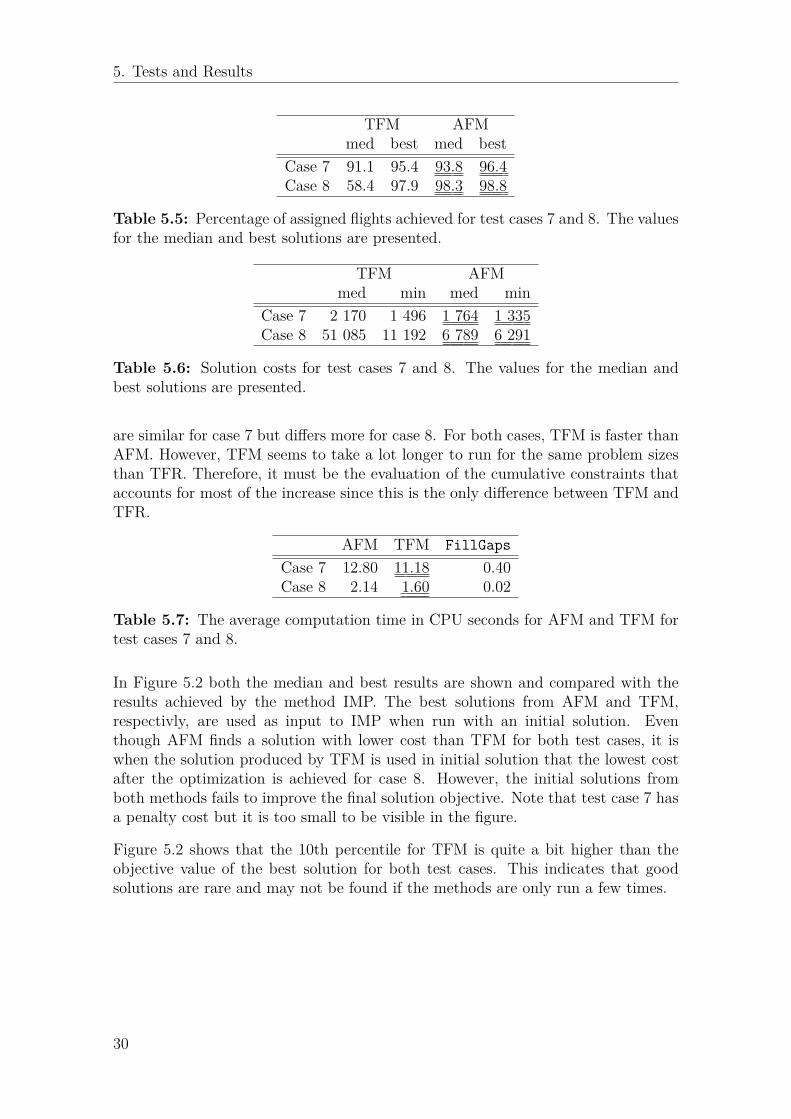
TFM AFMmed best med best

Case 7 91.1 95.4 93.8 96.4Case 8 58.4 97.9 98.3 98.8

Table 5.5: Percentage of assigned flights achieved for test cases 7 and 8. The valuesfor the median and best solutions are presented.

TFM AFMmed min med min

Case 7 2 170 1 496 1 764 1 335Case 8 51 085 11 192 6 789 6 291

Table 5.6: Solution costs for test cases 7 and 8. The values for the median andbest solutions are presented.

are similar for case 7 but differs more for case 8. For both cases, TFM is faster thanAFM. However, TFM seems to take a lot longer to run for the same problem sizesthan TFR. Therefore, it must be the evaluation of the cumulative constraints thataccounts for most of the increase since this is the only difference between TFM andTFR.

AFM TFM FillGapsCase 7 12.80 11.18 0.40Case 8 2.14 1.60 0.02

Table 5.7: The average computation time in CPU seconds for AFM and TFM fortest cases 7 and 8.

In Figure 5.2 both the median and best results are shown and compared with theresults achieved by the method IMP. The best solutions from AFM and TFM,respectivly, are used as input to IMP when run with an initial solution. Eventhough AFM finds a solution with lower cost than TFM for both test cases, it iswhen the solution produced by TFM is used in initial solution that the lowest costafter the optimization is achieved for case 8. However, the initial solutions fromboth methods fails to improve the final solution objective. Note that test case 7 hasa penalty cost but it is too small to be visible in the figure.

Figure 5.2 shows that the 10th percentile for TFM is quite a bit higher than theobjective value of the best solution for both test cases. This indicates that goodsolutions are rare and may not be found if the methods are only run a few times.

30

5. Tests and Results

0

500

1000

1500

2000

2500

3000

med min med min TFM

&

AFM

&

TFM AFM IMP IMP IMP LB

Co

st

Case 7

Penalty

Unassigned

Connection

0

10000

20000

30000

40000

50000

60000

med min med min TFM

&

AFM

&

TFM AFM IMP IMP IMP LB

Co

st

Case 8

Unassigned

Connection

Figure 5.2: Bar plot with the different methods for test cases 7 and 8, the blackinterval represents the 10th and 90th percentiles, respectivly, of the total cost; seedescription in the text.

31

5. Tests and Results

32

6Discussion and Conclusion

This thesis presents some variations of fast heuristics to create initial solutions to thetail assignment problem. These solutions can be used to warm start an improvementmethod as well as to produce legal solutions fast for other use cases.

The developed methods consist of first applying the method called FillGaps thatassigns tasks between pre-assignments and then applying one of the appending meth-ods Aircraft First Random (AFR), Aircraft First Sort (AFS), Task First Sort (TFS),Task First Random (TFR), Task First Maintenance (TFM), and Aircraft First Main-tenance (AFM). FillGaps and AFM use variants of heuristic version of Depth FirstSearch (DFS) and the other methods use greedy algorithms.

The methods are chosen with short running time as the main criteria. Since theproduced solutions are to be improved by an existing improvement method, there isno need to develop an own improvement algorithm. If some more complex techniquethan greedy algorithms and DFS was used, even more tasks could probably beassigned but it would be to the detriment of running time. This thesis focused onthe fastest possible approaches.

The evaluation was performed on eight test cases, six without hard cumulativeconstraints and two with cumulative constraints. The methods performed well withrespect to the percentage of tasks assigned. The goal was to assign 95% of thetasks and this was achieved with some method for all except one test case. Onthe other hand, the results of actually using the solutions as initial solutions to theimprovement method (IMP) showed that it is not always better to use an initialsolution. For the cases for which IMP produced a solution with all tasks assignedwithout an initial solution, using an initial solution may even produce a worse finalsolution. However, for the cases where IMP without initial solution did not assignall of the tasks, the results of using an initial solution improved the final solution.It should, however, be noted that more test cases are needed before this kind ofconclusions can be drawn with certainty.

The objective value was not improved for the cases with hard cumulative constraints.Therefore, the methods for hard cumulative constraints need to be improved to beuseful. However, AFM reached the goal for percentage of tasks assigned both forthe minimum and median cost solution found for one test case and TFM reachedthe goal for both test cases with the minimum cost solution. Since the methods

33

6. Discussion and Conclusion

achieve a high number of assigned tasks, it might be possible to tune Jeppesen’soptimizer (using another improvement method than IMP) so that good results canbe obtained with these methods as well.

For the improvement method to benefit from an initial solution, it might not beenough to have a high number of assigned tasks in the initial solution. Instead,there seems to be some other criteria. From the results presented in this thesis it ishard to draw any conclusions about why the final solution is not always improved byusing an initial solution. But since the planning period is divided into time windows,it is possible that there is no way to cover all tasks in the interval with the fixedstart and end positions that comes from the initial solution, while it may be possibleto cover all tasks if the end position is not fixed. Therefore, it might be necessaryto consider some other criteria while constructing the initial solutions.

The method IMP is just one out of many ways to run Jeppesen’s optimizer. Forexample, IMP sweeps through the planning period only once, while it is more com-mon to do several sweeps through the planning period. There might also be otherconfigurations for the column generation part of the optimizer that can make betteruse of the initial solutions.

The solutions generated by the methods proposed in this thesis could also be usedas initial solutions to other methods. For example, stochastic methods like Simu-lated Annealing and Particle Swarm Optimization, which Jamili et al. [9] use forother airline optimization problems, can benefit from the solutions produced by themethods proposed in this thesis. The solutions can also be used when designing therules for a new airline customer to quickly get an idea of how the different rules andcosts influence the solution.

Our methods are very fast, all of them are run in less than half a minute even for aninstance with 112 aircraft. This indicates that it is possible to use our methods alsofor even larger instances. It also opens up for the possibility to run several differentmethods and to run each method several times.

Our results show that the orders of tasks and aircraft are important, and to get thebest out of these methods, they should be run multiple times with different orderings.A possible improvement in the future is to find a sorting/ordering principle thatworks well for all cases or at least for a well defined set of problem instances. Somesorting schemes were not included in this thesis, since the preliminary results showedthat they did not work very well. For methods based on the task-first principle, thisincludes sorting on arrival time, using the reverse order every second iteration, andchoosing the task with the lowest connection cost.

The methods also need more testing in order to determine which method that per-forms best for which type of cases. There is also a need to test if there is a significantdifference in the quality of the final solution of using the best or worst solution foundby a method. Since the objective value of the final solution did not seem to corre-late with the objective value of the initial solution, it might be the case that it isunnecessary to run the initial methods multiple times if the improvement method

34

6. Discussion and Conclusion

ends up in a good solution also with a ”bad” initial solution.

Even though our evaluation has been focused on comparing the different append-ing algorithms, one should not forget the important part played by the methodFillGaps. This method takes care of the pre-assigned tasks that the time windowheuristic sometimes can have difficulties with.

The final conclusion is that the methods developed in this thesis create solutionswith many assigned tasks fast, but more testing and analysis is needed to know howand when these initial solutions should be used.

35

6. Discussion and Conclusion

36

Bibliography

[1] M. Grönkvist, “The Tail Assignment Problem”, PhD thesis, Chalmers Univer-sity of Technology, 2005.

[2] P. Belobaba, A. R. Odoni, and C. Barnhart, The Global Airline Industry,English, Second edition. Chichester, West Sussex, UK: John Wiley & Sons,2015.

[3] S. Gabteni and M. Grönkvist, “Combining column generation and constraintprogramming to solve the tail assignment problem”, Annals of OperationsResearch, vol. 171, no. 1, pp. 61–76, 2009. doi: 10.1007/s10479-008-0379-1.

[4] O. Khaled, M. Minoux, V. Mousseau, S. Michel, and X. Ceugniet, “A compactoptimization model for the tail assignment problem”, European Journal ofOperational Research, vol. 264, no. 2, pp. 548–557, 2018. doi: 10.1016/j.ejor.2017.06.045.

[5] A. Sarac, R. Batta, and C. M. Rump, “A branch-and-price approach for op-erational aircraft maintenance routing”, European Journal of Operational Re-search, vol. 175, no. 3, pp. 1850–1869, 2006. doi: 10.1016/j.ejor.2004.10.033.

[6] N. Safaei and A. K. Jardine, “Aircraft routing with generalized maintenanceconstraints”, Omega, 2017. doi: 10.1016/J.OMEGA.2017.08.013.

[7] A. Kasirzadeh, M. Saddoune, and F. Soumis, “Airline crew scheduling: models,algorithms, and data sets”, EURO Journal on Transportation and Logistics,vol. 6, no. 2, pp. 111–137, 2017. doi: 10.1007/s13676-015-0080-x.

[8] S. Ruther, N. Boland, F. G. Engineer, and I. Evans, “Integrated Aircraft Rout-ing, Crew Pairing, and Tail Assignment: Branch-and-Price with Many PricingProblems”, Transportation Science, vol. 51, no. 1, pp. 177–195, 2017. doi:10.1287/trsc.2015.0664.

[9] A. Jamili, “A robust mathematical model and heuristic algorithms for inte-grated aircraft routing and scheduling, with consideration of fleet assignmentproblem”, Journal of Air Transport Management, vol. 58, pp. 21–30, 2017.doi: 10.1016/J.JAIRTRAMAN.2016.08.008.

37

Bibliography

[10] G.-F. Deng and W.-T. Lin, “Ant colony optimization-based algorithm for air-line crew scheduling problem”, Expert Systems with Applications, vol. 38, no. 5,pp. 5787–5793, 2011. doi: 10.1016/J.ESWA.2010.10.053.

[11] M. M. Wahde, Biologically inspired optimization methods : an introduction.WIT Press, 2008, p. 218.

[12] Y.-C. Lai, D.-C. Fan, and K.-L. Huang, “Optimizing rolling stock assignmentand maintenance plan for passenger railway operations”, Computers & Indus-trial Engineering, vol. 85, pp. 284–295, 2015.

[13] Z. A. Juman and M. A. Hoque, “An efficient heuristic to obtain a better ini-tial feasible solution to the transportation problem”, Applied Soft ComputingJournal, vol. 34, pp. 813–826, 2015. doi: 10.1016/j.asoc.2015.05.009.

[14] J. Joubert and S. Claasen, “A sequential insertion heuristic for the initialsolution to a constrained vehicle routing problem”, ORiON: The Journal ofORSSA, vol. 22, no. 1, pp. 105–116, 2006. doi: 10.5784/22-1-36.

[15] P. C. Guedes and D. Borenstein, “Column generation based heuristic frame-work for the multiple-depot vehicle type scheduling problem”, Computers andIndustrial Engineering, vol. 90, pp. 361–370, 2015. doi: 10.1016/j.cie.2015.10.004.

[16] W. Dai, X. Sun, and S. Wandelt, “Finding feasible solutions for multi-com-modity flow problems”, in Chinese Control Conference, CCC, vol. 2016-Augus,IEEE, 2016, pp. 2878–2883. doi: 10.1109/ChiCC.2016.7553801.

[17] S. Boyd and L. Vandenberghe, Convex Optimization. Cambridge, United King-dom: Cambridge University Press, 2004.

[18] T. C. Hu and A. B. Kahng, “Introduction to the Simplex Method”, in Linearand Integer Programming Made Easy, Cham: Springer International Publish-ing, 2016, pp. 39–60. doi: 10.1007/978-3-319-24001-5_4.

[19] D. A. Spielman and S.-H. Teng, “Smoothed analysis of algorithms: Why thesimplex algorithm usually takes polynomial time”, J. ACM, vol. 51, no. 3,pp. 385–463, 2004. doi: 10.1145/990308.990310.

[20] R. Vershynin, “Beyond Hirsch conjecture: Walks on random polytopes andsmoothed complexity of the simplex method”, English, SIAM Journal on Com-puting, vol. 39, no. 2, pp. 646–678, 2009.

[21] J. Matoušek and B. Gärtner, “Not only the simplex method”, in Understand-ing and Using Linear Programming, Berlin, Heidelberg: Springer Berlin Hei-delberg, 2007, pp. 105–130. doi: 10.1007/978-3-540-30717-4_7.

[22] ——, “Integer programming and LP relaxation”, in Understanding and UsingLinear Programming, Berlin, Heidelberg: Springer Berlin Heidelberg, 2007,pp. 29–40. doi: 10.1007/978-3-540-30717-4.

[23] G. Nemhauser and L. Wolsey, “Integer programming”, in Handbooks in Op-erations Research and Management Science: Optimization, G. Nemhauser, A.Rinnooy Kan, and M. Todd, Eds. Amsterdam, The Netherlands: Elsevier Sci-ence Publishers, 1989.

38

Bibliography

[24] J. Desrosiers and M. E. Lübbecke, “A primer in column generation”, in ColumnGeneration, G. Desaulniers, J. Desrosiers, and M. M. Solomon, Eds. Boston,MA: Springer US, 2005, pp. 1–32. doi: 10.1007/0-387-25486-2_1.

[25] S. Irnich and G. Desaulniers, “Shortest path problems with resource con-straints”, in Column Generation, G. Desaulniers, J. Desrosiers, and M. M.Solomon, Eds. Boston, MA: Springer US, 2005, pp. 33–65. doi: 10.1007/0-387-25486-2_2.

[26] M. E. Lübbecke and J. Desrosiers, “Selected topics in column generation”,Operations Research, vol. 53, no. 6, pp. 1007–1023, 2005. doi: 10 . 2307 /25146936.

[27] “Artificial variables”, in Encyclopedia of Operations Research and ManagementScience, S. I. Gass and M. C. Fu, Eds., Boston, MA: Springer US, 2013, pp. 83–83. doi: 10.1007/978-1-4419-1153-7_200964.

[28] C. Barnhart, E. L. Johnson, G. L. Nemhauser, M. W. P. Savelsbergh, andP. H. Vance, “Branch-and-price: Column generation for solving huge integerprograms”, Operations Research, vol. 46, no. 3, pp. 316–329, 1998. doi: 10.1287/opre.46.3.316.

[29] “Greedy algorithm”, in Encyclopedia of Operations Research and ManagementScience, S. I. Gass and M. C. Fu, Eds., Boston, MA: Springer US, 2013,pp. 666–667. doi: 10.1007/978-1-4419-1153-7_200276.

[30] G. Brassard and P. Bratley, “Greedy algorithms”, in Fundamentals of algo-rithmics. Englewood Cliffs: Prentice Hall, 1996, vol. 33.

[31] E. Andersson, A. Forsman, S. E. Karisch, N. Kohl, and A Sørensson, “Problemsolving in airline operations”, Carmen Research and Technology Report CRTR-0404, Carmen Systems AB, Gothenburg, Sweden, 2004.

[32] M. Grönkvist, “Accelerating column generation for aircraft scheduling usingconstraint propagation”, Computers & Operations Research, vol. 33, no. 10,pp. 2918–2934, 2006. doi: 10.1016/J.COR.2005.01.017.

[33] J. Kleinberg and E. Tardos, Algorithm Design, English, Pearson New Interna-tional Edition. Harlow, United Kingdom: Pearson Education M.U.A, 2013.

39

Bibliography

40